SUPPLEMENTARY MATERIALS - International Union of ...
9
SUPPLEMENTARY MATERIALS Statistical analysis of multipole-model-derived structural parameters and charge-density properties from high-resolution X-ray diffraction experiments Radosław Kamiński, a * §‡ Sławomir Domagała, a * § Katarzyna N. Jarzembska, a‡ Anna A. Hoser, a W. Fabiola Sanjuan- Szklarz, a Matthias J. Gutmann, b Anna Makal, a Maura Malińska, a Joanna M. Bąk, a Krzysztof Woźniak a a Department of Chemistry, University of Warsaw, Pasteura 1, 02-093 Warszawa, Poland b ISIS Neutron and Muon Source, Science and Technology Facilities Council, Rutherford Appleton Laboratory, Harwell Oxford, Didcot, Oxfordshire OX11 0QX, UK * Corresponding authors: Radosław Kamiński ([email protected]), Sławomir Domagała ([email protected]) § Both authors contributed equally to this work ‡ Current address: Department of Chemistry, University at Buffalo, The State University of New York, Buffalo, NY 14260-3000, USA
Transcript of SUPPLEMENTARY MATERIALS - International Union of ...

SUPPLEMENTARY MATERIALS
Statistical analysis of multipole-model-derived structural
parameters and charge-density properties from
high-resolution X-ray diffraction experiments
Radosław Kamiński,a*§‡ Sławomir Domagała,a*§ Katarzyna N. Jarzembska,a‡
Anna A. Hoser,a W. Fabiola Sanjuan-Szklarz,a Matthias J. Gutmann,b
Anna Makal,a Maura Malińska,a Joanna M. Bąk,a Krzysztof Woźniaka
a Department of Chemistry, University of Warsaw, Pasteura 1, 02-093 Warszawa, Poland b ISIS Neutron and Muon Source, Science and Technology Facilities Council, Rutherford Appleton
Laboratory, Harwell Oxford, Didcot, Oxfordshire OX11 0QX, UK
* Corresponding authors: Radosław Kamiński ([email protected]),
Sławomir Domagała ([email protected])
§ Both authors contributed equally to this work
‡ Current address: Department of Chemistry, University at Buffalo, The State University
of New York, Buffalo, NY 14260-3000, USA

S1. Additional figures
Figure S1. Sum of residual density maps across all 13 high-resolution measurements (C1-O2-C1(1−x, 1−y,
1−z) plane; contours at 0.05 e·Å−3, blue lines – positive values, red – negative).
oxa01 oxa02

oxa03 oxa04
Figure S2. Fractal dimension plots for all oxalic acid datasets (horizontal axis – residual density (ϱres)
given in e·Å−1; vertical axis – fractal dimension (df)).
oxa05 oxa06

oxa07 oxa08
Figure S2 (continued). Fractal dimension plots for all oxalic acid datasets.
oxa09 oxa10

oxa11 oxa12
Figure S3 (continued). Fractal dimension plots for all oxalic acid datasets.
oxa13
Figure S4 (continued). Fractal dimension plots for all oxalic acid datasets.
S2. Additional tables
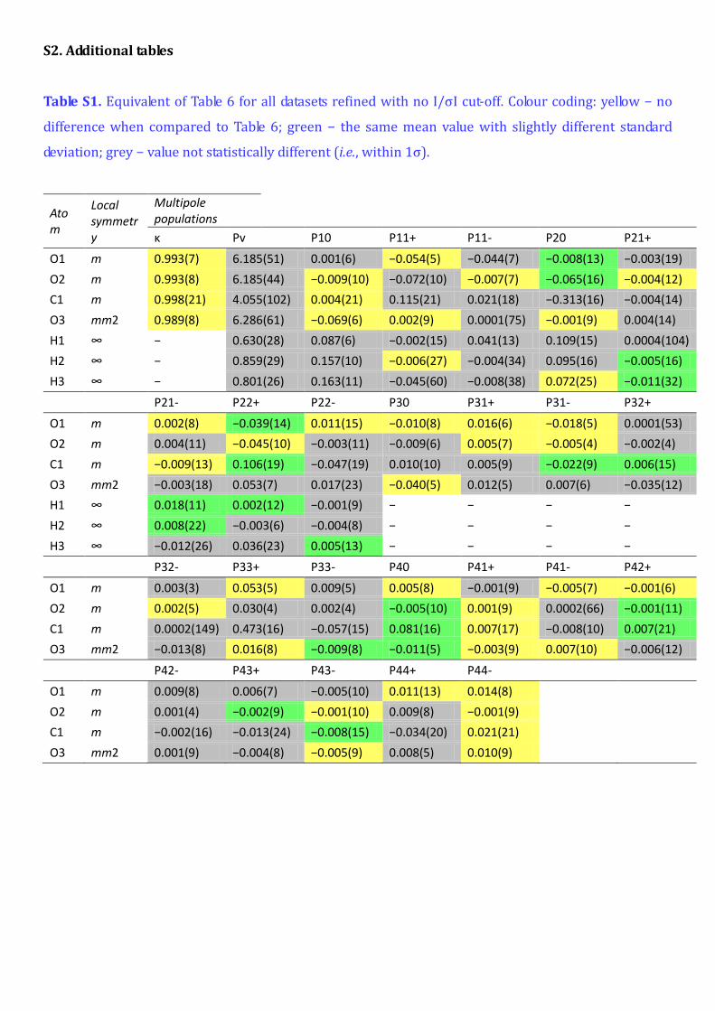
Table S1. Equivalent of Table 6 for all datasets refined with no I/σI cut-off. Colour coding: yellow − no
difference when compared to Table 6; green − the same mean value with slightly different standard
deviation; grey − value not statistically different (i.e., within 1σ).
Atom
Local symmetry
Multipole populations κ Pv P10 P11+ P11- P20 P21+
O1 m 0.993(7) 6.185(51) 0.001(6) −0.054(5) −0.044(7) −0.008(13) −0.003(19) O2 m 0.993(8) 6.185(44) −0.009(10) −0.072(10) −0.007(7) −0.065(16) −0.004(12) C1 m 0.998(21) 4.055(102) 0.004(21) 0.115(21) 0.021(18) −0.313(16) −0.004(14) O3 mm2 0.989(8) 6.286(61) −0.069(6) 0.002(9) 0.0001(75) −0.001(9) 0.004(14) H1 ∞ − 0.630(28) 0.087(6) −0.002(15) 0.041(13) 0.109(15) 0.0004(104) H2 ∞ − 0.859(29) 0.157(10) −0.006(27) −0.004(34) 0.095(16) −0.005(16) H3 ∞ − 0.801(26) 0.163(11) −0.045(60) −0.008(38) 0.072(25) −0.011(32)
P21- P22+ P22- P30 P31+ P31- P32+
O1 m 0.002(8) −0.039(14) 0.011(15) −0.010(8) 0.016(6) −0.018(5) 0.0001(53) O2 m 0.004(11) −0.045(10) −0.003(11) −0.009(6) 0.005(7) −0.005(4) −0.002(4) C1 m −0.009(13) 0.106(19) −0.047(19) 0.010(10) 0.005(9) −0.022(9) 0.006(15) O3 mm2 −0.003(18) 0.053(7) 0.017(23) −0.040(5) 0.012(5) 0.007(6) −0.035(12) H1 ∞ 0.018(11) 0.002(12) −0.001(9) − − − − H2 ∞ 0.008(22) −0.003(6) −0.004(8) − − − − H3 ∞ −0.012(26) 0.036(23) 0.005(13) − − − − P32- P33+ P33- P40 P41+ P41- P42+
O1 m 0.003(3) 0.053(5) 0.009(5) 0.005(8) −0.001(9) −0.005(7) −0.001(6) O2 m 0.002(5) 0.030(4) 0.002(4) −0.005(10) 0.001(9) 0.0002(66) −0.001(11) C1 m 0.0002(149) 0.473(16) −0.057(15) 0.081(16) 0.007(17) −0.008(10) 0.007(21) O3 mm2 −0.013(8) 0.016(8) −0.009(8) −0.011(5) −0.003(9) 0.007(10) −0.006(12)
P42- P43+ P43- P44+ P44-
O1 m 0.009(8) 0.006(7) −0.005(10) 0.011(13) 0.014(8) O2 m 0.001(4) −0.002(9) −0.001(10) 0.009(8) −0.001(9) C1 m −0.002(16) −0.013(24) −0.008(15) −0.034(20) 0.021(21) O3 mm2 0.001(9) −0.004(8) −0.005(9) 0.008(5) 0.010(9)

Table S2. Numerical values for plots presented in Figure 5. L denotes the sample mean of the Laplacian
(L=2ϱ); d denotes distance from the BCP to the atomic centre (positive values indicate direction
towards O1 atom, negative towards the C1 atom; BCP position is given in bold).
d / Å ϱ / e·Å−3 sϱ / e·Å−3 sϱ/ϱ / e·Å−3 L / e·Å−5 sL / e·Å−5 sL/L / e·Å−5
–0.39 581.81 97.42 0.17 –1621335.15 1257389.63 0.8 –0.36 297.47 49.04 0.16 –139347.46 68987.32 0.5 –0.33 153.54 24.95 0.16 –13211.02 10499.58 0.8 –0.30 79.99 12.79 0.16 5712.14 1247.51 0.2 –0.27 42.18 6.58 0.16 6529.53 393.04 0.1 –0.24 22.68 3.39 0.15 4573.64 505.86 0.1 –0.21 12.65 1.74 0.14 2801.75 367.59 0.1 –0.18 7.52 0.89 0.12 1607.87 231.07 0.1 –0.15 4.92 0.45 0.09 879.44 136.42 0.2 –0.12 3.63 0.23 0.06 456.29 77.68 0.2 –0.09 3.00 0.12 0.04 218.47 43.03 0.2 –0.06 2.71 0.08 0.03 88.90 23.21 0.3 –0.03 2.58 0.06 0.02 21.09 12.16 0.6 0.00 2.50 0.06 0.02 –29.53 2.70 0.1 0.03 2.52 0.06 0.02 –27.03 3.48 0.1 0.06 2.55 0.06 0.02 –23.06 4.09 0.2 0.09 2.60 0.06 0.02 –18.78 4.29 0.2 0.12 2.68 0.06 0.02 –14.86 4.23 0.3 0.15 2.77 0.06 0.02 –11.75 4.00 0.3 0.18 2.90 0.08 0.03 –9.82 3.65 0.4 0.21 3.07 0.09 0.03 –9.48 3.24 0.3 0.24 3.27 0.11 0.03 –11.16 2.88 0.3 0.27 3.52 0.14 0.04 –15.45 2.84 0.2 0.30 3.81 0.16 0.04 –22.97 3.52 0.2 0.33 4.14 0.20 0.05 –34.37 5.00 0.1 0.36 4.51 0.23 0.05 –49.90 6.96 0.1 0.39 4.92 0.26 0.05 –68.73 8.78 0.1 0.42 5.35 0.29 0.05 –87.16 9.43 0.1 0.45 5.80 0.32 0.06 –94.71 11.51 0.1 0.48 6.28 0.36 0.06 –65.67 33.92 0.5 0.51 6.82 0.43 0.06 59.07 100.76 1.7 0.54 7.60 0.62 0.08 410.35 260.44 0.6 0.57 9.05 1.14 0.13 1268.98 617.24 0.5 0.60 12.34 2.52 0.20 3211.42 1372.72 0.4 0.63 20.38 6.02 0.30 7317.73 2849.51 0.4 0.66 40.23 14.65 0.36 15124.00 5211.35 0.3 0.69 89.02 35.77 0.40 25932.98 6246.96 0.2 0.72 208.48 87.42 0.42 14857.36 22022.64 1.5 0.75 501.47 214.71 0.43 –264747.89 311371.42 1.2 0.78 1226.40 533.26 0.43 –14769727.38 27897210.07 1.9

Table S3. Definitions of parameters used to quantify electrostatic potential (ESP) mapped onto
molecular surfaces (Murray & Politzer, 1998; Murray et al., 2000).
Quantity Description
VSri ESP value on the molecular surface computed at point ri
n+ number of grid points corresponding to the positive value of ESP
n- number of grid points corresponding to the negative value of ESP
VS,max maximal value of the surface ESP value
VS,min minimal value of the surface ESP value
VS+=1n+i=1n+VS+ri positive average of the potential over the surface
VS-=1n-i=1n-VS-ri negative average of the potential over the surface
VS=1n++n-i=1n+VS+ri+i=1n-VS-ri overall average of the potential over the surface
Π=1n++n-i=1n++n-VSri-VS average deviation of VSri
σ+2=1n+i=1n+VS+ri-VS+2 positive variance of VSri
σ-2=1n-i=1n-VS-ri-VS-2 negative variance of VSri
σtot2=σ+2+σ-2 total variance of VSri
ν=σ+2σ-2σtot22 degree of balance between the positive and negative surface potentials