www.sciencemag.org/cgi/content/full/science.aaf4388/DC1

Supplementary Materials for

Designer nanoscale DNA assemblies programmed from the top down

Rémi Veneziano, Sakul Ratanalert, Kaiming Zhang, Fei Zhang, Hao Yan, Wah Chiu, Mark Bathe*

*Corresponding author. Email: mark.bathe@mit.edu

Published 26 May 2016 on Science First Release

DOI: 10.1126/science.aaf4388

This PDF file includes:

Materials and Methods Supplementary Text S1 to S7 Figs. S1 to S59 Tables S1 to S5 Captions for tables S6 to S27 Captions for movies S1 to S7 References (57–64)

Other Supplementary Materials for this manuscript include the following: (available at www.sciencemag.org/cgi/content/full/science.aaf4388/DC1)

Tables S6 to S27 Movies S1 to S7 DAEDALUS Software Package (zip file)

2

Materials and Methods:

Design Algorithm

Specifying geometry

The goal of this work is to design and synthesize scaffolded DNA origami structures with

a top-down approach: given a target 3D structure of specified size and geometry (Fig. 1), the

algorithm will route a single-stranded scaffold throughout the entire geometry and generate the

required staple strands needed to experimentally fold the structure. We term our algorithm

DAEDALUS (DNA Origami Sequence Design Algorithm for User-defined Structures) (see

online Supporting Software and http://daedalus-dna-origami.org) for its ability to fully

automatically generate the scaffold routing and complementary staple sequences for an arbitrary

3D shape. 3D geometries are specified using a closed surface that is discretized using a

polyhedral mesh. In order to specify the geometry for scaffold routing, the spatial coordinates of

all vertices, the edge connectivities between vertices, and the faces to which vertices belong must

be provided (Fig. 2A and Fig. S1A to S1B). These may be provided manually, or through a file

format that specifies polygonal geometry, such as the Polygon File Format (PLY),

Stereolithography (STL), or Virtual Reality Modeling Language (WRL). As explained in more

detail below, any closed, orientable surface network can serve as input to the algorithm (Fig. 2

and Fig. S4 to S5). Provided in the code is a parser to convert PLY files into the required inputs.

In addition to the preceding spatial information, the desired minimum edge length, in bp, must be

specified for the structure (e.g. 31 or 42 bp). Each edge of the final scaffolded DNA origami

structure must be a multiple of 10.5 bp, rounded up or down to the nearest nucleotide, with a

minimum of 31 bp. For structures with equal edge lengths throughout the geometry, such as

Platonic, Archimedean, or Johnson solids, the desired minimum edge length simply becomes the

length for every edge. For other geometries, rounding edge lengths may be required, resulting in

some possible deviation between the specified target structure and final design. In these cases,

the desired minimum edge length is assigned to the shortest edge and the other edges are scaled

and rounded appropriately. When using the automated rounding to generate edge lengths, the

user is advised to verify that edge lengths are satisfactory before proceeding to the scaffold

routing procedure. If they are not, or if the user desires a structure with the same edge and face

connectivities but different edge lengths (e.g. modifying a regular tetrahedron into an irregular

tetrahedron), the user can edit and specify each edge length individually, so long as the lengths

meet the requirements mentioned above.

3

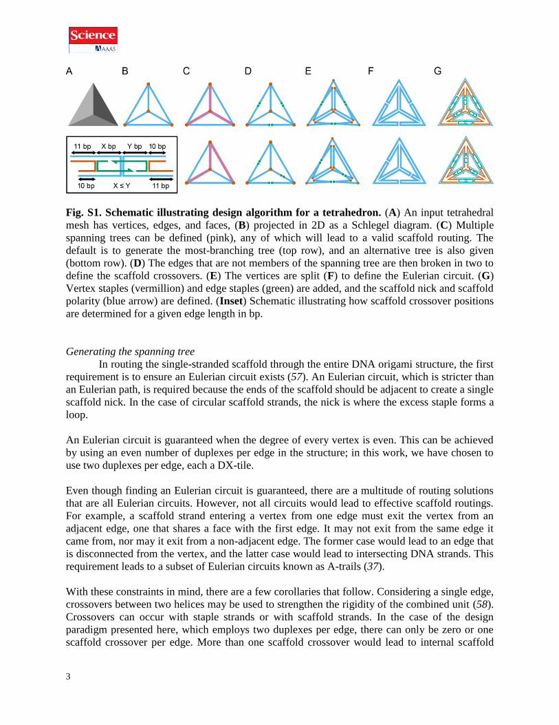
Fig. S1. Schematic illustrating design algorithm for a tetrahedron. (A) An input tetrahedral

mesh has vertices, edges, and faces, (B) projected in 2D as a Schlegel diagram. (C) Multiple

spanning trees can be defined (pink), any of which will lead to a valid scaffold routing. The

default is to generate the most-branching tree (top row), and an alternative tree is also given

(bottom row). (D) The edges that are not members of the spanning tree are then broken in two to

define the scaffold crossovers. (E) The vertices are split (F) to define the Eulerian circuit. (G)

Vertex staples (vermillion) and edge staples (green) are added, and the scaffold nick and scaffold

polarity (blue arrow) are defined. (Inset) Schematic illustrating how scaffold crossover positions

are determined for a given edge length in bp.

Generating the spanning tree

In routing the single-stranded scaffold through the entire DNA origami structure, the first

requirement is to ensure an Eulerian circuit exists (57). An Eulerian circuit, which is stricter than

an Eulerian path, is required because the ends of the scaffold should be adjacent to create a single

scaffold nick. In the case of circular scaffold strands, the nick is where the excess staple forms a

loop.

An Eulerian circuit is guaranteed when the degree of every vertex is even. This can be achieved

by using an even number of duplexes per edge in the structure; in this work, we have chosen to

use two duplexes per edge, each a DX-tile.

Even though finding an Eulerian circuit is guaranteed, there are a multitude of routing solutions

that are all Eulerian circuits. However, not all circuits would lead to effective scaffold routings.

For example, a scaffold strand entering a vertex from one edge must exit the vertex from an

adjacent edge, one that shares a face with the first edge. It may not exit from the same edge it

came from, nor may it exit from a non-adjacent edge. The former case would lead to an edge that

is disconnected from the vertex, and the latter case would lead to intersecting DNA strands. This

requirement leads to a subset of Eulerian circuits known as A-trails (37).

With these constraints in mind, there are a few corollaries that follow. Considering a single edge,

crossovers between two helices may be used to strengthen the rigidity of the combined unit (58).

Crossovers can occur with staple strands or with scaffold strands. In the case of the design

paradigm presented here, which employs two duplexes per edge, there can only be zero or one

scaffold crossover per edge. More than one scaffold crossover would lead to internal scaffold

4

loops that are disconnected from the rest of the scaffold. Therefore, a scaffold strand entering an

edge from a vertex can either leave the edge from the same vertex or from the other vertex.

Similarly, considering a single vertex, at least one edge connected to the vertex must have zero

scaffold crossovers. If all edges at the vertex have scaffold crossovers, an internal loop would be

generated. However, a scaffold crossover is in fact necessary. Considering a single face or any

closed circuit of edges, at least one edge must have one scaffold crossover. If all edges have no

scaffold crossovers, an internal loop would be generated.

Because scaffold crossovers are required, one manner of designing a polyhedron would be to

identify all the possible locations for a scaffold crossover, and then select which locations shall

have the scaffold crossover based on the above criteria. Doing so would lead to a valid structure,

and is a viable approach for designing arbitrary scaffolded DNA origami (59). However, the

number of locations for a scaffold crossover scales with the size of the object, making the

algorithm computationally intractable for many structures. In particular, structures with the same

symmetry have similar routing patterns regardless of size. A general approach cannot take

advantage of this and would iterate through all possibilities of scaffold crossovers, when in fact

the solution is predictable and could be obtained more efficiently.

Given the above restrictions on the number and location of edges with a scaffold crossover for

DNA origami objects, solving the scaffold routing can be mapped to a simpler problem:

classifying edges as either possessing zero scaffold crossovers or possessing one scaffold

crossover.

From the above criteria, the edges with zero scaffold crossovers must connect to every vertex,

and there can be no cycles of edges with zero scaffold crossovers. This implies that there are V –

1 edges with zero scaffold crossovers, where V is the number of vertices, and the remaining

edges have one scaffold crossover. The edges with zero scaffold crossovers meet the definition

of a spanning tree of a network.

Thus, solving the scaffold routing problem is identical to solving for a spanning tree of the

structure, where each possible spanning tree corresponds to a unique scaffold routing. Fig. S1C

presents two different spanning trees for a tetrahedron. Given a network, Prim’s algorithm can be

used to find the minimum weight spanning tree. If, as in this case, all edges are weighted the

same, Prim’s algorithm will generate a breadth-first search spanning tree, one with the most

branches. It has been shown for 2D nets that branching trees self-assemble more reliably than

more linear trees (36). Fig. S2 shows the default spanning trees used to route the scaffold for

each of the 45 objects in Fig. 2.

Note that with this spanning tree algorithm, there are no restrictions on the topology of the

network. Any arrangement of nodes and edges can be routed with an Eulerian circuit, using a

spanning tree to define the placement of scaffold crossovers. However, the use of faces allows

A-trails to be defined more easily in automation, and some networks do not have clearly defined

faces, i.e. planar faces with an unambiguous outward normal. One example of this would be

eight cubes stacked in a 2x2x2 formation, for a total of 27 vertices. The faces around the vertex

at the center are not clearly arranged, making several scaffold routings about that vertex possible.

As such, the current algorithm is well-suited for any closed surface, which includes not only

5

spherical topologies but also toroidal polyhedra and other geometries with holes (Fig. 2 and Fig

S4).

Fig. S2. Spanning trees of input polyhedra generated by the algorithm. The spanning tree

(pink) of each input polyhedron (shown as a Schlegel diagram in blue) defines the edges that do

not have scaffold crossovers. The remaining edges will have scaffold crossovers added during

the scaffold routing procedure.

Adding pseudo-nodes and scaffold routing

Once the spanning tree has been determined, the graph needs to be converted to an

Eulerian circuit. First, for each edge that is not in the spanning tree, a pair of pseudo-nodes is

added to split the edge into two halves, each corresponding to one side of a scaffold crossover

(Fig. S1D).

Next, for each vertex in the graph, a set of pseudo-nodes is added to replace the vertex node. A

vertex of degree N has N edges emerging from it and N faces between them. For each face, a

pseudo-node is placed that joins the two bordering edges and disconnects them from the other

edges. After all pseudo-nodes are placed for all vertices, the original vertex nodes are no longer

part of the graph, and each edge is now bounded on both ends by pseudo-nodes. This defines the

Eulerian circuit through which the scaffold will be routed (Fig. S1E and S1F).

This circuit defines two possible routings: one that routes around faces clockwise, and one that

routes around faces counterclockwise, relative to the outward normal. The direction of the

scaffold is chosen to run counterclockwise around each face, so that for convex vertices (the

majority of cage vertices) the major grooves of the duplexes at each vertex point inward to

minimize electrostatic repulsion of the backbone (Fig. 5D) (38). The undirected graph is

converted to a directed graph to implement this directional choice.

At this point, the lengths of the edges are introduced into the algorithm; the spanning tree and

pseudo-node addition are only geometry-specific, independent of size. The scaffold nick

6

position, for simplicity, is chosen to always be located on an edge without scaffold crossovers,

on the duplex far from staple nicks and crossovers. Using Prim’s algorithm, this edge will have

Vertex #1 as one of its endpoints, since with the most-branching default all edges connected to

Vertex #1 are members of the spanning tree. Marking this 5’-end as scaffold base #1, each of the

scaffold bases are subsequently numbered with knowledge of the edge lengths and routing

scheme, all while keeping track of their relative position on their edge. Note that for each edge,

the 5’-end overhangs the 3’-end by one nucleotide to ensure that all staple and scaffold

crossovers remain perpendicular to the helical axes. The half-edges, namely those edges that are

split by the scaffold crossover, have lengths that are pre-determined by some simplifying

assumptions. The scaffold crossover is placed as close to the center as possible, with a

convention set here to have a preference towards the lower-index vertex if needed. Therefore, the

length of the scaffold segment that spans any particular edge is given deterministically by the

algorithm (Fig. S1H and Table S1).

Table S1. Determining the location of a scaffold crossover for a given edge length. The

variables X and Y are defined for the region hybridized by edge staples, ignoring the 10- and 11-

bp regions on either side hybridized by vertex staples. By convention set here, X ≤ Y, where X is

the region closer to the lower-index vertex, and Y is the region closer to the higher-index vertex.

X + Y + 21 = L

X ≤ Y

L = 21n + {10 or 11}

L = 21n + 0

Edge length L is

even

Off-center by 0.5, Y = X + 1

(e.g. L = 52: X = 15, Y = 16)

Off-center by 5.5, Y = X + 11

(e.g. L = 42: X = 5, Y = 16)

Edge length L is

odd

Off-center by 0, Y = X

(e.g. L = 31: X = 5, Y = 5)

Off-center by 5, Y = X + 10

(e.g. L = 63: X = 16, Y = 26)

Adding staple strands and generating sequence

Each scaffold base now has two pieces of information associated with it: one index

number indicates its position on the scaffold strand, and set of numbers indicate its spatial

location: the edge, the duplex, and the position from the 5’ end. In routing the staple strands, the

latter set is used to identify which bases in the staples are paired with which bases in the scaffold,

then the former index number is assigned to the staples accordingly.

There are three categories of staple strands, each with their own prescribed pattern: staples on

vertices, staples on edges with scaffold crossovers, and staples on edges without scaffold

crossovers. The staples on vertices pair with the first 10–11 nucleotides of each duplex abutting

the vertex, with poly-T bulges of length 5 crossing between edges. There are two varieties of

vertex staple designs implemented: one system uses single crossovers in some places to ensure

that there is 10–11 bp of continuous duplex for high specificity and binding strength, and the

other, more traditional, system uses double crossovers everywhere, leading to a minimum of 5 bp

7

of continuous duplex (3, 12). For the structures synthesized and characterized in this work, the

former paradigm is used, as the higher binding strength was found to create a more cooperative

transition at a higher temperature (Fig. S19). The pattern of staple routing depends on the degree

of the vertex, ensuring that each staple length is 52- or 78-nucleotides (nt) long for ease of

synthesis.

0, if mod3 0

2, if mod3 1

1, if mod3 2

n

a n

n

(Eq. 1)

2

3

n ab

(Eq. 2)

where a is the number of 52-nt staples at the vertex,

b is the number of 78-nt staples at the vertex, and

n is the degree of the vertex.

The edge staples pair with the intermediate nucleotides between vertex staples. For the edges

with scaffold crossovers, two 31–32-nt staples are placed across the scaffold crossover, together

occupying a 15–16-nt region on either side of the crossover for sufficiently strong binding. The

remainder of scaffold has 42-nt staples placed to create staple crossovers every 21 base pairs,

with a 20- or 22-nt staple in the case of a 10- or 11-nt remainder. The edges without scaffold

crossovers simply follow this latter pattern, filling with as many 42-nt staples that can fit and

using a 20- or 22-nt staple when necessary (Fig. S1G).

The minimum edge length allowed in this design paradigm is 31 bp. Any smaller value will

place a scaffold crossover 5 nt away from the end of an edge (in the vertex staple region), which

may lead to low folding yield. However, the rules described above are applicable to lengths of 42

bp and greater, and they need to be modified slightly for 31- and 32-bp edges. First, a 31-/32-bp

edge has 21 bp occupied by vertex staples, leaving 10 or 11 bp for edge staples. Therefore, in

both types of edges, a 20- or 22-bp staple is placed with a single crossover on one side, because a

staple nick in the middle would coincide with the scaffold crossover. This in turn means that the

single-crossover vertex staple design may lead to a missing crossover, so to be safe the double-

crossover vertex staple design is always used in any structure with a 31- or 32-bp edge present.

After all the staples are placed, each staple is denoted by a vector of numbers, with each value

corresponding to the scaffold nucleotide to which it is base-paired. The input or generated

scaffold sequence is then used to match base identities (A, T, G, or C) to the corresponding

scaffold number assuming Watson-Crick base-pairing. If no sequence is provided, a segment of

M13pm18 is used by default if the required scaffold length is less than or equal to 7,249 nt, and a

sequence is randomly generated if the required length is greater. Finally, this list of staple

sequences is output for synthesis.

Predicting atomic-level 3D structure

The position and orientation of each base pair is calculated by interpolating between the

two ends of the edge that it resides on, with a perpendicular shift from the central edge axis of 1

8

nm, which is approximately half the interhelical distance for an anti-parallel crossover. The edge

is assumed to lie in a plane with a normal vector defined by the sum of the unit normal vectors of

the two neighboring faces.

There are several models that can be used to define the locations of the ends of the edges. In the

models described here, the DX-tile edges may be assumed to be two parallel cylinders with

combined width 4 nm (2 nm interhelical distance and 2 nm duplex diameter). This can be further

simplified to a rectangle with width 4 nm, with the line of the edge serving as a central axis (Fig.

S3A). In the ideal case, the corners of these rectangles meet, since the scaffold exits and enters

the edge from these locations. The widths of the rectangles together would form an N-sided

regular polygon, because they have the same sides and have equal angles between them. The

perpendicular distance from the center of this polygon and an edge (the beginning of the

interpolation) is the inradius of this polygon. From the inradius, the distance between the vertex

and the beginning of the DX-tile edge is determined using the sum of the face angles. If the

multi-arm DX-tile were flat, this would be equivalent to the inradius.

2

tot

s r

(Eq. 3)

where s is the distance between the vertex and the beginning of the DX-tile edge,

r is the inradius of the polygon formed by the widths of the tiles, and

tot is the sum of all face angles at the vertex.

For regular N-sided polygons,

cot2

wr

N

(Eq. 4)

where w is the combined width of the DX-tile (40 Å).

This first model (Eq. 4) assumes that all vertices have equal angles. There are some structures,

however, whose edges do not meet at regular angles, such as the Archimedean solids. In these

cases, depending on the convention used to define the length of the inradius, there will be

backbone stretches and/or nucleotide overlaps. The second model investigated minimizes

nucleotide overlap, while the third minimizes backbone stretch (Fig. S3A, center and right of

each panel). Based on the cryo-electron microscopy (cryo-EM) data for the cuboctahedron (Fig.

5D and Fig. S3B), a representative Archimedean solid, the size of the object is best fit with the

third model when backbone stretches are minimized (Fig. S3A), where the inradius is calculated

based on the largest face angle (Eq. 5).

maxcot2 2

wr

(Eq. 5)

where max is the largest face angle. Note that this general equation applies to regular N-sided

polygons as well, since max 2 / N , so this third model is applied for all structures.

9

For structures with concave vertices, where 2tot , to obey the convention that all edge axes

meet at a single point, we define s r as a corner case extension of the third model, creating a

sphere of radius r that defines the edge boundaries.

Fig. S3. Comparison of competing models for predicting 3D atomic structure of DX-based

polyhedra. (A) There are several conventions by which to define the inradius of the vertex

(circle shown in black for a four-way and three-way junction, respectively), which determines

how the distance between the vertex and the beginning of the DX-tile edge (rectangles, centered

on the edges, represented by dotted lines, which meet at a single point). For vertices with equal

face angles (the first model, left of each panel), the definition is clear, as it is the inradius of the

regular polygon defined by the widths. However, for vertices with unequal face angles, the

convention may be to prefer backbone stretches over nucleotide overlap (the second model,

center of each panel), or the reverse (the third model, right of each panel). (B) The

cuboctahedron cryo-EM map fit with the structural model using the second model, the center

convention from (A). The model is large enough such that the overlap is minimal when the map

and model are centered (left); a maximum correlation of 0.45 is achieved by shifting off-center

(right). Based on this data, the third model, which minimizes backbone stretch, is applied for all

structures.

10

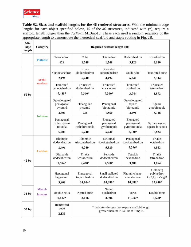
Table S2. Sizes and scaffold lengths for the 46 rendered structures. With the minimum edge

lengths for each object specified below, 15 of the 46 structures, indicated with (*), require a

scaffold length longer than the 7,249-nt M13mp18. These each used a random sequence of the

appropriate length to demonstrate the theoretical scaffold and staple routing in Fig. 2B.

Min

edge

length

Category Required scaffold length (nt)

52 bp

Platonic Tetrahedron

624

Cube

1,248

Octahedron

1,248

Dodecahedron

3,120

Icosahedron

3,120

Archi-

medean

Cuboctahedron

2,496

Icosi-

dodecahedron

6,240

Rhombi-

cuboctahedron

4,492

Snub cube

6,240

Truncated cube

3,744

Truncated

cuboctahedron

7,488*

Truncated

dodecahedron

9,360*

Truncated

icosahedron

9,360*

Truncated

octahedron

3,744

Truncated

tetrahedron

1,872

Johnson

Gyroelongated

pentagonal

pyramid

2,600

Triangular

pyramid

936

Pentagonal

bipyramid

1,560

Gyroelongated

square

bipyramid

2,496

Square

gyrobicupola

3,328

Pentagonal

orthocupola-

rotunda

5,200

Pentagonal

orthobirotunda

6,240

Elongated

pentagonal

gyrobicupola

6,240

Elongated

pentagonal

gyrobirotunda

8,320*

Gyroelongated

square bicupola

5,824

42 bp

Catalan

Rhombic

dodecahedron

2,496

Rhombic

triacontahedron

6,240

Deltoidal

icositetrahedron

5,520

Pentagonal

icositetrahedron

7,296*

Triakis

octahedron

4,512

Disdyakis

dodecahedron

7,584*

Triakis

icosahedron

9,420*

Pentakis

dodecahedron

7,560*

Tetrakis

hexahedron

3,288

Triakis

tetrahedron

1,884

Miscel-

laneous

Heptagonal

bipyramid

3,808

Enneagonal

trapezohedron

14,004*

Small stellated

dodecahedron

10,080*

Rhombic hexe-

contahedron

10,080*

Goldberg

polyhedron

G(2,1), dk5dgD

17,640*

31 bp Double helix

9,812*

Nested cube

3,016

Nested

octahedron

3,396

Torus

11,532*

Double torus

8,520*

52 bp

Reinforced

cube

2,136

* indicates designs that require scaffold length

greater than the 7,249-nt M13mp18

11

Fig. S4. Atomic models of scaffolded DNA origami nanoparticles with nonspherical

topologies. (i) Nested cube; (ii) nested octahedron; (iii) torus; and (iv) double torus. Particles not

shown to scale; see Table S2 for sizes and scaffold lengths.

12

Fig. S5. Atomic models of scaffolded DNA origami nanoparticles with spherical topologies.

(A) (i) Tetrahedron; (ii) cube; (iii) octahedron; (iv) dodecahedron; (v) icosahedron; and (vi)

cuboctahedron. Particles not shown to scale; see Table S2 for sizes and scaffold lengths.

13

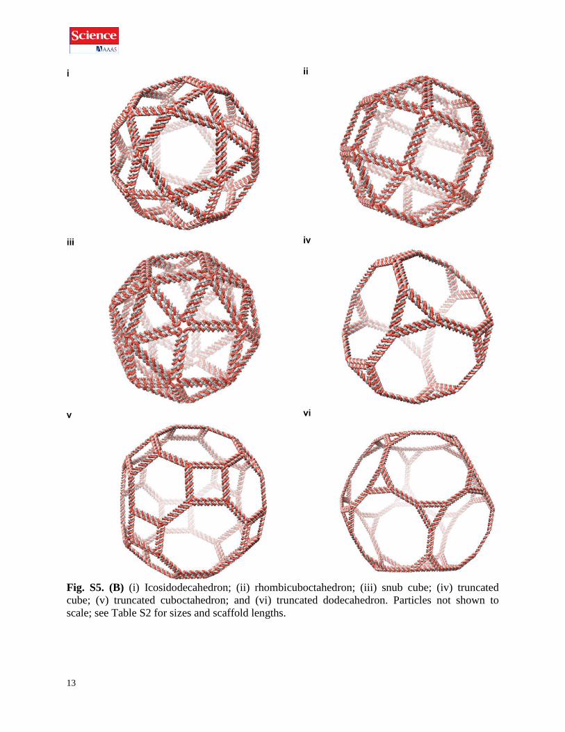
Fig. S5. (B) (i) Icosidodecahedron; (ii) rhombicuboctahedron; (iii) snub cube; (iv) truncated

cube; (v) truncated cuboctahedron; and (vi) truncated dodecahedron. Particles not shown to

scale; see Table S2 for sizes and scaffold lengths.

14

Fig. S5. (C) (i) Truncated icosahedron; (ii) truncated octahedron; (iii) truncated tetrahedron; (iv)

gyroelongated pentagonal pyramid; (v) triangular pyramid; and (vi) pentagonal bipyramid.

Particles not shown to scale; see Table S2 for sizes and scaffold lengths.

15

Fig. S5. (D) (i) Gyroelongated square bipyramid; (ii) square gyrobicupola; (iii) pentagonal

orthocupolarotunda; (iv) pentagonal orthobirotunda; (v) elongated pentagonal gyrobicupola; and

(vi) elongated pentagonal gyrobirotunda. Particles not shown to scale; see Table S2 for sizes and

scaffold lengths.

16

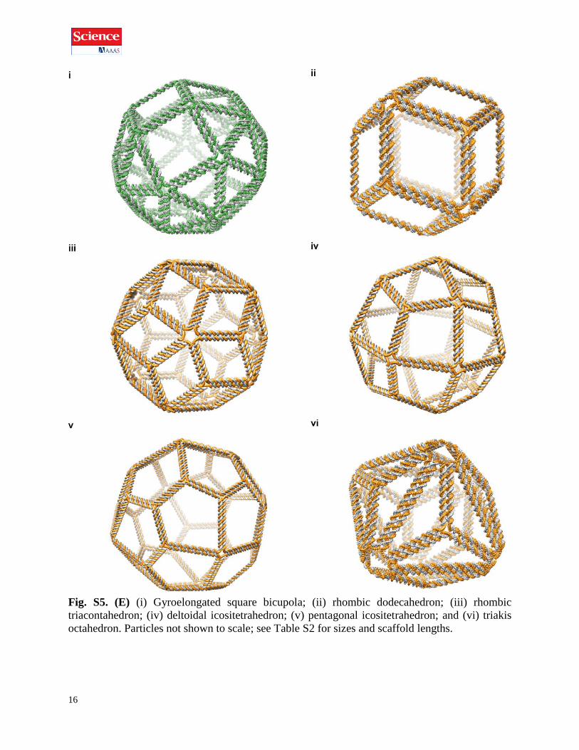
Fig. S5. (E) (i) Gyroelongated square bicupola; (ii) rhombic dodecahedron; (iii) rhombic

triacontahedron; (iv) deltoidal icositetrahedron; (v) pentagonal icositetrahedron; and (vi) triakis

octahedron. Particles not shown to scale; see Table S2 for sizes and scaffold lengths.

17

Fig. S5. (F) (i) Disdyakis dodecahedron; (ii) triakis icosahedron; (iii) pentakis dodecahedron;

(iv) tetrakis hexahedron; (v) triakis tetrahedron; and (vi) heptagonal bipyramid. Particles not

shown to scale; see Table S2 for sizes and scaffold lengths.

18

Fig. S5. (G) (i) Enneagonal trapezohedron; (ii) small stellated dodecahedron; (iii) rhombic

hexecontahedron; (iv) Goldberg polyhedron G(2,1); (v) double helix; and (vi) reinforced cube.

Particles not shown to scale; see Table S2 for sizes and scaffold lengths.

19

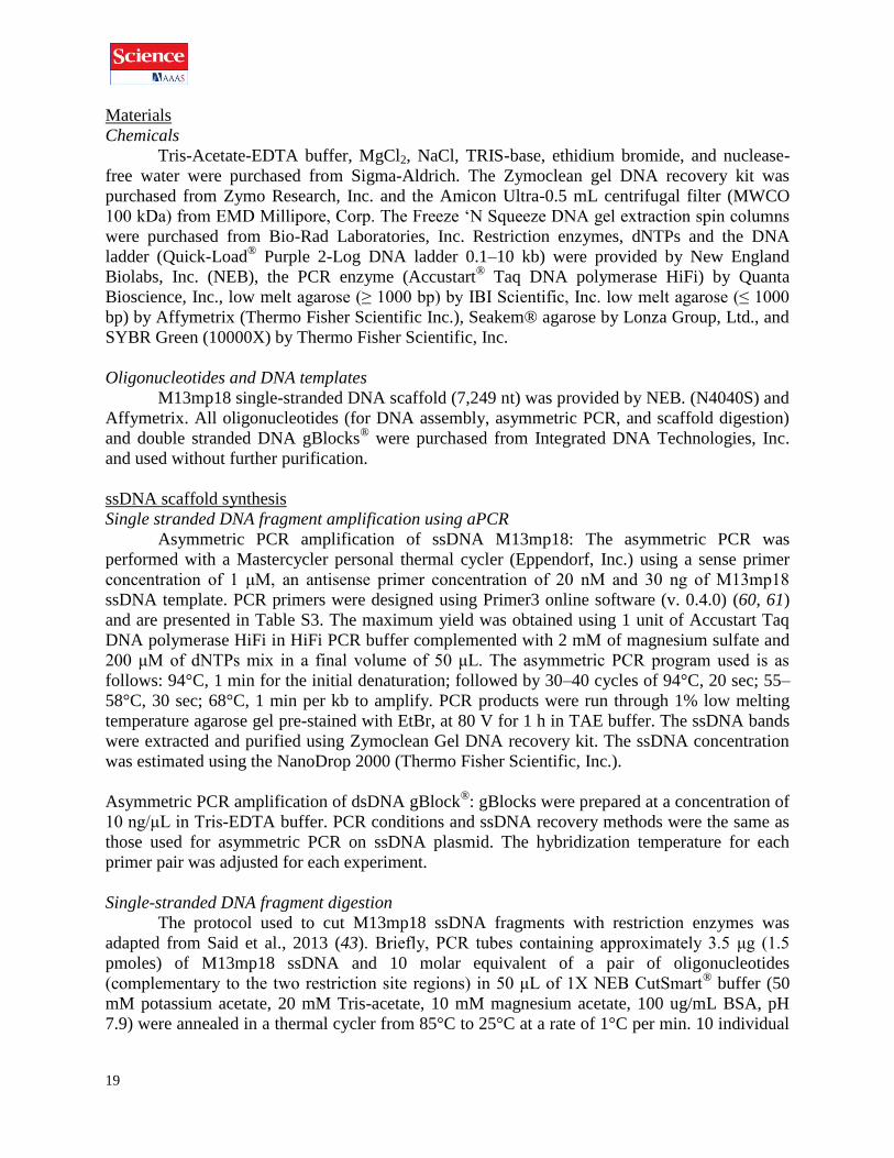
Materials

Chemicals

Tris-Acetate-EDTA buffer, MgCl2, NaCl, TRIS-base, ethidium bromide, and nuclease-

free water were purchased from Sigma-Aldrich. The Zymoclean gel DNA recovery kit was

purchased from Zymo Research, Inc. and the Amicon Ultra-0.5 mL centrifugal filter (MWCO

100 kDa) from EMD Millipore, Corp. The Freeze ‘N Squeeze DNA gel extraction spin columns

were purchased from Bio-Rad Laboratories, Inc. Restriction enzymes, dNTPs and the DNA

ladder (Quick-Load®

Purple 2-Log DNA ladder 0.1–10 kb) were provided by New England

Biolabs, Inc. (NEB), the PCR enzyme (Accustart® Taq DNA polymerase HiFi) by Quanta

Bioscience, Inc., low melt agarose (≥ 1000 bp) by IBI Scientific, Inc. low melt agarose (≤ 1000

bp) by Affymetrix (Thermo Fisher Scientific Inc.), Seakem® agarose by Lonza Group, Ltd., and

SYBR Green (10000X) by Thermo Fisher Scientific, Inc.

Oligonucleotides and DNA templates

M13mp18 single-stranded DNA scaffold (7,249 nt) was provided by NEB. (N4040S) and

Affymetrix. All oligonucleotides (for DNA assembly, asymmetric PCR, and scaffold digestion)

and double stranded DNA gBlocks® were purchased from Integrated DNA Technologies, Inc.

and used without further purification.

ssDNA scaffold synthesis

Single stranded DNA fragment amplification using aPCR

Asymmetric PCR amplification of ssDNA M13mp18: The asymmetric PCR was

performed with a Mastercycler personal thermal cycler (Eppendorf, Inc.) using a sense primer

concentration of 1 μM, an antisense primer concentration of 20 nM and 30 ng of M13mp18

ssDNA template. PCR primers were designed using Primer3 online software (v. 0.4.0) (60, 61)

and are presented in Table S3. The maximum yield was obtained using 1 unit of Accustart Taq

DNA polymerase HiFi in HiFi PCR buffer complemented with 2 mM of magnesium sulfate and

200 μM of dNTPs mix in a final volume of 50 μL. The asymmetric PCR program used is as

follows: 94°C, 1 min for the initial denaturation; followed by 30–40 cycles of 94°C, 20 sec; 55–

58°C, 30 sec; 68°C, 1 min per kb to amplify. PCR products were run through 1% low melting

temperature agarose gel pre-stained with EtBr, at 80 V for 1 h in TAE buffer. The ssDNA bands

were extracted and purified using Zymoclean Gel DNA recovery kit. The ssDNA concentration

was estimated using the NanoDrop 2000 (Thermo Fisher Scientific, Inc.).

Asymmetric PCR amplification of dsDNA gBlock®: gBlocks were prepared at a concentration of

10 ng/μL in Tris-EDTA buffer. PCR conditions and ssDNA recovery methods were the same as

those used for asymmetric PCR on ssDNA plasmid. The hybridization temperature for each

primer pair was adjusted for each experiment.

Single-stranded DNA fragment digestion

The protocol used to cut M13mp18 ssDNA fragments with restriction enzymes was

adapted from Said et al., 2013 (43). Briefly, PCR tubes containing approximately 3.5 μg (1.5

pmoles) of M13mp18 ssDNA and 10 molar equivalent of a pair of oligonucleotides

(complementary to the two restriction site regions) in 50 μL of 1X NEB CutSmart® buffer (50

mM potassium acetate, 20 mM Tris-acetate, 10 mM magnesium acetate, 100 ug/mL BSA, pH

7.9) were annealed in a thermal cycler from 85°C to 25°C at a rate of 1°C per min. 10 individual

20

tubes were pooled and 100 units (10 μL) of each restriction enzyme was added directly to the

mix. The mix was aged at 37°C for 3 h. After incubation, each sample was concentrated to 50 μL

using an Amicon Ultra-0.5 mL centrifugal filter (MWCO 100 kDa), and run through a 1% low

melting temperature agarose gel electrophoresis pre-stained with EtBr. Purification of ssDNA

was performed with Zymoclean gel DNA recovery kit. Final ssDNA concentration was

determined using the NanoDrop 2000.

21

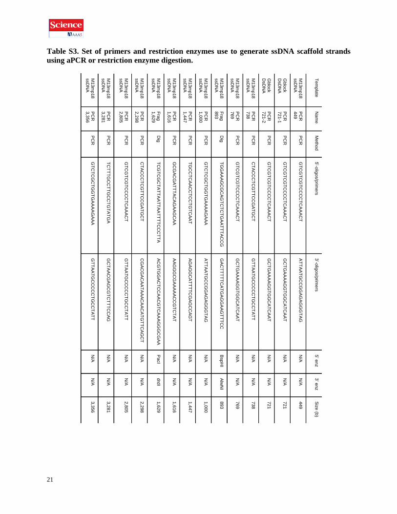
Table S3. Set of primers and restriction enzymes use to generate ssDNA scaffold strands

using aPCR or restriction enzyme digestion.

Tem

pla

te

Nam

e

Meth

od

5’-o

ligos/p

rime

rs

3’-o

ligos/p

rime

rs

5’ e

nz

3’ e

nz

Siz

e (b

)

M13m

p18

ssD

NA

P

CR

449

P

CR

G

TC

GT

CG

TC

CC

CT

CA

AA

CT

A

TT

AA

TG

CC

GG

AG

AG

GG

TA

G

N/A

N

/A

449

Gblo

ck

DsD

NA

P

CR

721

-1

PC

R

GT

CG

TC

GT

CC

CC

TC

AA

AC

T

GC

TG

AA

AA

GG

TG

GC

AT

CA

AT

N

/A

N/A

721

Gblo

ck

DsD

NA

P

CR

721

-2

PC

R

GT

CG

TC

GT

CC

CC

TC

AA

AC

T

GC

TG

AA

AA

GG

TG

GC

AT

CA

AT

N

/A

N/A

721

M13m

p18

ssD

NA

P

CR

738

P

CR

C

TA

CC

CT

CG

TT

CC

GA

TG

CT

G

TT

AA

TG

CC

CC

CT

GC

CT

AT

T

N/A

N

/A

738

M13m

p18

ssD

NA

P

CR

769

P

CR

G

TC

GT

CG

TC

CC

CT

CA

AA

CT

G

CT

GA

AA

AG

GT

GG

CA

TC

AA

T

N/A

N

/A

769

M13m

p18

ssD

NA

F

rag

893

D

ig

TG

GA

AA

GC

GC

AG

TC

TC

TG

AA

TT

TA

CC

G

GA

CT

TT

TT

CA

TG

AG

GA

AG

TT

TC

C

BspH

I A

lwN

I 893

M13m

p18

ssD

NA

P

CR

1,0

00

P

CR

G

TC

TC

GC

TG

GT

GA

AA

AG

AA

A

AT

TA

AT

GC

CG

GA

GA

GG

GT

AG

N

/A

N/A

1,0

00

M13m

p18

ssD

NA

P

CR

1,4

47

P

CR

T

GC

CT

CA

AC

CT

CC

TG

TC

AA

T

AG

AG

GC

AT

TT

TC

GA

GC

CA

GT

N

/A

N/A

1,4

47

M13m

p18

ssD

NA

P

CR

1,6

16

P

CR

G

CG

AC

GA

TT

TA

CA

GA

AG

CA

A

AA

GG

GC

GA

AA

AA

CC

GT

CT

AT

N

/A

N/A

1,6

16

M13m

p18

ssD

NA

F

rag

1,6

29

D

ig

TC

GT

CG

CT

AT

TA

AT

TA

AT

TT

TC

CC

TT

A

AC

GT

GG

AC

TC

CA

AC

GT

CA

AA

GG

GC

GA

A

PacI

drd

I 1,6

29

M13m

p18

ssD

NA

P

CR

2,2

98

P

CR

C

TA

CC

CT

CG

TT

CC

GA

TG

CT

C

GA

CG

AC

AA

TA

AA

CA

AC

AT

GT

TC

AG

CT

N

/A

N/A

2,2

98

M13m

p18

ssD

NA

P

CR

2,8

05

P

CR

G

TC

GT

CG

TC

CC

CT

CA

AA

CT

G

TT

AA

TG

CC

CC

CT

GC

CT

AT

T

N/A

N

/A

2,8

05

M13m

p18

ssD

NA

P

CR

3,2

81

P

CR

T

CT

TT

GC

CT

TG

CC

TG

TA

TG

A

GC

TA

AC

GA

GC

GT

CT

TT

CC

AG

N

/A

N/A

3,2

81

M13m

p18

ssD

NA

P

CR

3,3

56

P

CR

G

TC

TC

GC

TG

GT

GA

AA

AG

AA

A

GT

TA

AT

GC

CC

CC

TG

CC

TA

TT

N

/A

N/A

3,3

56

22

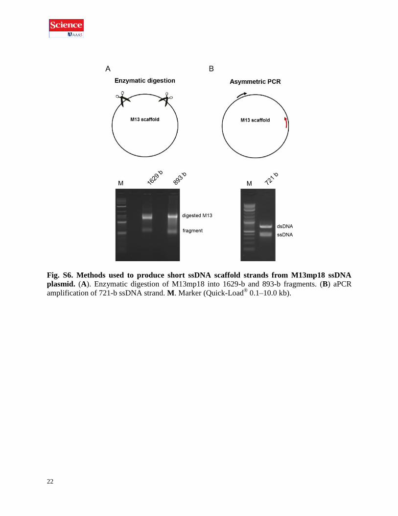
Fig. S6. Methods used to produce short ssDNA scaffold strands from M13mp18 ssDNA

plasmid. (A). Enzymatic digestion of M13mp18 into 1629-b and 893-b fragments. (B) aPCR

amplification of 721-b ssDNA strand. M. Marker (Quick-Load® 0.1–10.0 kb).

23

Fig. S7. Agarose gel electrophoresis of the scaffolds prepared by restriction enzyme

digestion. Gel electrophoresis shows high purity of the two ssDNA scaffolds generated by this

method. M. Marker (Quick-Load® 0.1–10.0 kb).

aPCR compared with single-stranded DNA fragment digestion

The aPCR method used here achieves higher quantities of scaffold with a smaller amount

of starting material than the digestion of M13mp18 using restriction enzymes. Briefly, to obtain

3 pmoles of purified product, 5 pmoles of M13mp18 are required using the digestion method

while only 0.012 pmoles are needed for aPCR amplification. With aPCR it is also possible to

generate many different scaffold lengths, whereas digestion relies on restriction site positions.

Fig. 3 and Table S3 lists the primers used for aPCR amplification, which can be combined as

desired to achieve a diverse array of scaffold sizes without generating new primers for each

custom length. The final quantity produced in a 50 μL PCR reaction tube is dependent on the

fragment size and sequences, ranging between 1.5–4.5 pmoles.

Folding and purification of DNA origami objects

DNA origami assembly

DNA origami annealing reactions were realized in 50 μL reaction tubes containing the

different ssDNA scaffolds in a 5–40 nM concentration range diluted in Tris-Acetate EDTA-

MgCl2 buffer (40 mM Tris, 20 mM acetic acid, 2 mM EDTA, 12 mM MgCl2, pH 8.0). The

nested cube was folded in the presence of 20 mM Mg2+

. To ensure correct folding and to

maximize yield, staple strand mixes were added in a 10–20X molar excess. Annealing was

performed in a Mastercycler personal thermal cycler (Eppendorf, Inc.) with the following

program: 95°C for 5 min, 80–75°C at 1°C per 5 min, 75–30°C at 1°C per 15 min, and 30–25°C

at 1°C per 10 min.

24

Purification of DNA origami objects

For AFM and cryo-EM characterization, DNA origami objects were purified using the

Amicon Ultra-0.5 mL centrifugal filter (MWCO 100 kDa). Briefly, fresh origami solutions were

washed three times with TAE-Mg2+

(12 mM MgCl2) buffer to remove excess of staple strands

using low speed centrifugation (1000 g). Origami objects purified are stored at 4°C prior to being

used for further characterization.

Buffer exchange and stability experiments

Buffer exchange

DNA origami objects were folded in TAE-Mg2+

buffer (12 mM MgCl2) and washed one

time with TAE-Mg2+

(12 mM MgCl2) buffer using Amicon Ultra-0.5 mL centrifugal filter

(MWCO 100 kDa) and subsequently washed three times with the new stability buffer (TAE,

PBS, or DMEM + FBS).

Stability experiments

The stabilities of DNA origami objects in TAE, PBS, or DMEM FluoroBrite (0.35%

BSA, 1% Penicillin/Streptomycin, 1% L-Glutamine) buffer complemented with 2% dialyzed

fetal bovine serum (dFBS) or 10% FBS were evaluated for 6 h. Because of the presence of large

macromolecules in DMEM, an extra step of purification was needed prior to imaging in order to

remove them and to avoid non-specific AFM signals (62). Briefly, the solutions of DNA

nanostructures incubated in DMEM were first run on a low melting temperature 1% agarose gel

and the bands corresponding to the DNA nanostructures were extracted and purified using a

Freeze ‘N SqueezeTM

DNA gel extraction spin column. Before AFM imaging, structures

extracted were concentrated using Amicon Ultra-0.5 centrifugal filter (MWCO 100 kDa) with

low speed centrifugation (1000 g).

Structural characterization methods

Agarose gel electrophoresis

Samples were loaded in 2% agarose gel in Tris-Acetate EDTA buffer supplemented with

12 mM MgCl2 and pre-stained with EtBr. Gels were run on a BioRad electrophoresis unit at 4°C

for 3–4 h under a constant voltage of 70 V. Gels were imaged using a Gene flash gel imager

(Syngene, Inc.), and yield was estimated by analyzing the band intensity with the Gel Analyzer

program in the ImageJ software (53).

Atomic force microscopy (AFM)

Samples for AFM were freshly annealed at a concentration of 5 nM in 40 μL TAE-Mg2+

(12 mM MgCl2) buffer and subsequently purified then concentrated using Amicon Ultra-0.5 mL

centrifugal filter (MWCO 100 kDa) to a final volume of 20–30 μL.

For AFM imaging, 1.5 μL samples were deposited onto freshly peeled mica (Ted Pella, Inc.) and

10 μL of 1x TAE-Mg2+

buffer were added to enlarge the solution drop to cover the whole mica

surface. 1.5 μL NiCl2 (100 mM) were added to the drop immediately. After leaving about 30

seconds for adsorption to the mica surface, 70 μL of 1x TAE-Mg2+

buffer were added to the

samples and an extra 40 μL of the same buffer were deposited on the AFM tip. The samples were

25

scanned in “ScanAssyst mode in fluid” using an AFM (Dimension FastScan, Bruker

Corporation, Inc.) with SCANASSYST-FLUID+ tips.

Cryo-EM

Cryo-EM samples were freshly prepared by annealing DNA objects at a scaffold

concentration of 20 nM in 50 μL TAE-Mg2+

(12 mM MgCl2) buffer. 15–25 tubes were prepared

for each structure, mixed and purified and finally concentrated using an Amicon column Ultra-

0.5 mL centrifugal filter (MWCO 100 kDa) to a final volume of 20–30 μL.

For cryo-EM imaging, 2 μL of the folded DNA nanostructure solution (~1 μM for the

tetrahedron and octahedron, ~750 nM for the nested cube and ~500 nM for the icosahedron,

cuboctahedron, and reinforced cube) were applied onto the glow-discharged 200-mesh R1.2/1.3

Quantifoil grid. Grids were then blotted for 1.5 sec and rapidly frozen in liquid ethane using a

Vitrobot Mark IV (FEI). All grids were screened on a JEM2200FS cryo-electron microscope

(JEOL) operated at 200 kV with in-column energy filter with a slit of 20 eV. Micrographs of the

icosahedron, tetrahedron, cuboctahedron, and octahedron were recorded with a direct detection

device (DDD) (DE-20 4k×5k camera, Direct Electron, LP) operating in movie mode at a

recording rate of 25 raw frames per second at 25,000× microscope magnification (corresponding

to a calibrated sampling of 2.51 Å per pixel) and a dose rate of ~21 electrons/sec/Å2 with a total

exposure time of 3 sec. Micrographs of the reinforced cube and the nested cube were recorded on

a 4k×4k CCD camera (Gatan, Inc) at 40,000× microscope magnification (corresponding to a

calibrated sampling of 2.95 Å per pixel) and a dose rate of ~20 electrons/sec/Å2 with a total

exposure time of 3 sec. A total of 180 images for the icosahedron, 91 images for the tetrahedron,

101 images for the cuboctahedron, 100 images for the octahedron, 36 images for the reinforced

cube, and 152 images for the nested cube were collected with a defocus range of ~1.5–4 μm.

Particle images recorded on DE-20 detector were motion corrected and radiation damage

compensated (24). The motion correction was done with running averages of three consecutive

frames using the DE_process_frames.py script (Direct Electron, LP). Single particle image

processing and 3D reconstruction was performed using the image processing software package

EMAN2 (54). EMAN2 was used for initial micrograph evaluation, particle picking, contrast

transfer function correction, 2D reference free class averaging, initial model building, and 3D

refinement. All initial models for the DNA origami objects were built from 2D reference-free

class averages. 3,650 particles for the icosahedron, 2,183 particles for the tetrahedron, 1,758

particles for the cuboctahedron, 2,678 particles for the octahedron, 915 particles for the

reinforced cube, and 2,008 particles for the nested cube were used for final refinement, applying

icosahedral, tetrahedral, octahedral, octahedral, tetrahedral, and octahedral symmetries,

respectively. Resolutions for the final maps were estimated using the 0.143 criterion of the

Fourier shell correlation (FSC) curve without any mask. A Gaussian low-pass filter was applied

to the final 3D maps displayed in the Chimera UCSF software package (55). Correlation of each

map with its corresponding atomic model is calculated by the UCSF Chimera fitmap function.

Tilt-pair validation for the cryo-EM map (56) was performed by collecting data at two

goniometer angles, 0° and -10°, for each region of the grid. The test was performed using the

e2tiltvalidate.py program in EMAN2. Additional details on the tilt-pair validation are provided in

Supplementary Table S3.

26

Quantitative PCR (qPCR) thermal analysis

qPCR analyses were performed in 384-well plate format using a Roche LightCycler®

480. A typical plate contained at least 3 replicates of each sample. Samples were complemented

with 1x final concentration of SYBR Green in a final volume of 20 μL. The scaffold

concentration used for the tetrahedron analysis was 80 nM and the concentrations of each strand

were adjusted to 1 μM for the three-way junction model. The annealing protocol used was

identical to the one used for DNA origami assembly. SYBR® Green fluorescence was monitored

over all experiments. Fluorescence curves obtained were analyzed using first-order derivatives to

identify transition temperatures.

27

Supplementary text

S1 Folding validation of DNA nanostructures with gel electrophoresis and AFM imaging

This section contains extra agarose gel electrophoresis characterization and the full AFM images

used in Fig. 4, showing validation and characterization of a set of DNA nanostructures designed

using our algorithm.

Fig. S8. Folding 52-bp edge-length DNA tetrahedron with full M13mp18 or with short

ssDNA (A) Tetrahedron folding under different MgCl2 concentration using the full M13mp18 as

scaffold (7,249 b). (B) Folding of Tetrahedron using ssDNA PCR 1,000 scaffold. M. Marker

(Quick-Load® 0.1–10.0 kb), sc. scaffold.

Fig. S9. Agarose gel electrophoresis of 31-bp edge-length DNA tetrahedron. The 31 bp

tetrahedron was folded in TAE-Mg2+

(12 mM MgCl2) buffer using the 450-nt ssDNA scaffold

amplified by aPCR. M. Marker (Quick-Load® 0.1–10.0 kb).

28

Fig. S10. Agarose gel electrophoresis of 42- and 52-bp edge-lengths DNA tetrahedra, PCR

721-1 and 721-2 scaffolds. The tetrahedra 42- and 52-bp were folded in TAE-Mg2+

(12 mM

MgCl2) buffer using the 721-1 (A) or 721-2 (B) scaffold amplified by aPCR from gBlock®

template. M. Marker (Quick-Load® 0.1–10.0 kb).

Fig. S11. Characterization of the 73-bp edge-length DNA nested cube. The DNA nested cube

was folded in TAE-Mg2+

(20 mM MgCl2) buffer using the 3,356-nt scaffold amplified using

aPCR and characterized using agarose gel electrophoresis and cryo-EM. M. Marker (Quick-

Load® 0.1–10.0 kb), sc. scaffold. Scale bars are 10 nm for the model and 20 nm for cryo-EM.

29

Fig. S12. AFM imaging of 63-bp edge-length DNA tetrahedron. Image size is 2 μm × 2 μm.

Fig. S13. AFM imaging of 52-bp edge-length DNA octahedron. Image size 2 μm × 2 μm.

30

Fig. S14. AFM imaging of 52-bp edge-length DNA icosahedron. Image size 2 μm × 2 μm.

Fig. S15. AFM imaging of 52-bp edge-length DNA pentagonal bipyramid. Image size 2 μm ×

2 μm.

31

Fig. S16. AFM imaging of 52-bp edge-length DNA cuboctahedron. Image size 2 μm × 2 μm.

Fig. S17. AFM imaging of 52-bp edge-length DNA reinforced cube. Image size 2 μm × 2 μm.

32

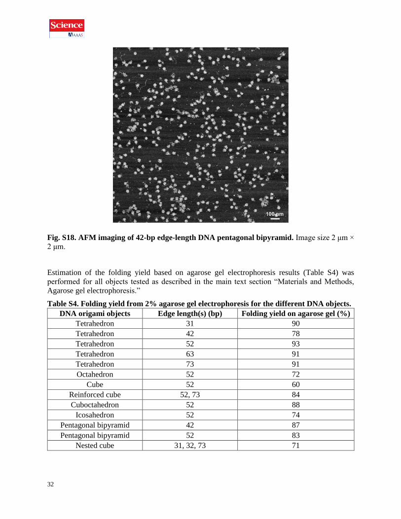
Fig. S18. AFM imaging of 42-bp edge-length DNA pentagonal bipyramid. Image size 2 μm ×

2 μm.

Estimation of the folding yield based on agarose gel electrophoresis results (Table S4) was

performed for all objects tested as described in the main text section “Materials and Methods,

Agarose gel electrophoresis.”

Table S4. Folding yield from 2% agarose gel electrophoresis for the different DNA objects.

DNA origami objects Edge length(s) (bp) Folding yield on agarose gel (%)

Tetrahedron 31 90

Tetrahedron 42 78

Tetrahedron 52 93

Tetrahedron 63 91

Tetrahedron 73 91

Octahedron 52 72

Cube 52 60

Reinforced cube 52, 73 84

Cuboctahedron 52 88

Icosahedron 52 74

Pentagonal bipyramid 42 87

Pentagonal bipyramid 52 83

Nested cube 31, 32, 73 71

33

S2 Vertex staple design comparison using qPCR

Fig. S19. Vertex staple design characterization on isolated vertex and 52-bp edge-length

DNA tetrahedron. (A) Proposed vertex staples design for 3-, 4-, 5-, and 6-way junctions. (B)

34

Comparison of our vertex staple design with previous models. (C) qPCR (raw data) and agarose

gel electrophoresis for vertex staple, isolated tiles (3-way junction). (D) Analysis of qPCR curve

using first derivatives to identify transition temperatures. (E) qPCR (raw data) and agarose gel

electrophoresis for different model of vertex staples version of tetrahedron 52-bp edge length.

(F) Analysis of qPCR curve using first derivatives to identify transition temperatures. M.

Marker, sc. Scaffold, N1. One nick model, N2. Two nick model, WOT. Without poly-T model,

SX. Single cross-over.

S3 Cryo-EM imaging and 3D reconstruction of DNA origami objects

To validate the 3D structures of the set of objects designed and folded we performed 3D cryo-

EM reconstruction. This section contains wide-view images used for each structure presented in

Fig. 4.

Fig. S20. Cryo-EM imaging of 63-bp edge-length DNA tetrahedron.

35

Fig. S21. Cryo-EM imaging of 52-bp edge-length DNA octahedron.

Fig. S22. Cryo-EM imaging of 52-bp edge-length DNA icosahedron.

36

Fig. S23. Cryo-EM imaging of 52-bp edge-length DNA pentagonal bipyramid.

Fig. S24. Cryo-EM imaging of 52-bp edge-length DNA cuboctahedron.

37

Fig. S25. Cryo-EM imaging of 52-bp edge-length DNA reinforced cube.

Fig. S26. Cryo-EM imaging of the 63-bp edge-length DNA tetrahedron at high density. This

cryo-EM image reveals that no aggregation occurs even at high nanoparticle density, obtained

using our methods to purify and concentrate samples for cryo-EM characterization.

38

Fig. S27. Cryo-EM imaging of the 73-bp edge-length DNA nested cube.

39

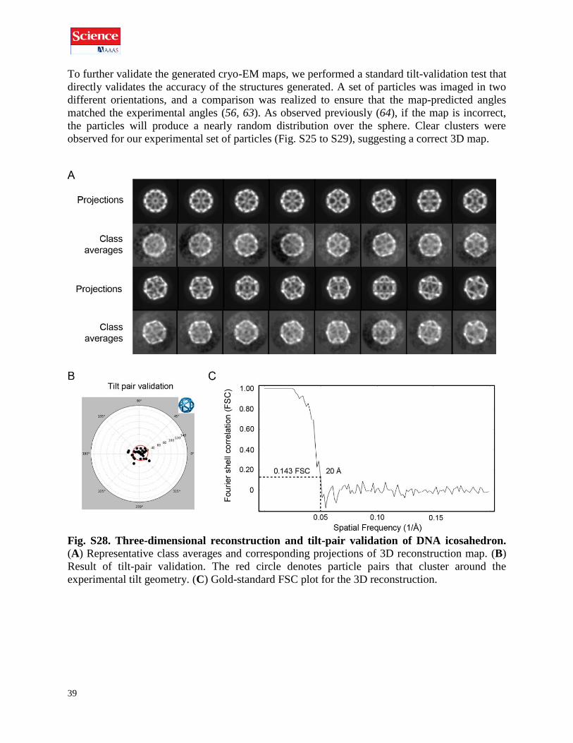
To further validate the generated cryo-EM maps, we performed a standard tilt-validation test that

directly validates the accuracy of the structures generated. A set of particles was imaged in two

different orientations, and a comparison was realized to ensure that the map-predicted angles

matched the experimental angles (56, 63). As observed previously (64), if the map is incorrect,

the particles will produce a nearly random distribution over the sphere. Clear clusters were

observed for our experimental set of particles (Fig. S25 to S29), suggesting a correct 3D map.

Fig. S28. Three-dimensional reconstruction and tilt-pair validation of DNA icosahedron.

(A) Representative class averages and corresponding projections of 3D reconstruction map. (B)

Result of tilt-pair validation. The red circle denotes particle pairs that cluster around the

experimental tilt geometry. (C) Gold-standard FSC plot for the 3D reconstruction.

40

Fig. S29. Three-dimensional reconstruction and tilt-pair validation of DNA tetrahedron.

(A) Representative class averages and corresponding projections of 3D reconstruction map. (B)

Result of tilt-pair validation. The red circle denotes particle pairs that cluster around the

experimental tilt geometry. (C) Gold-standard FSC plot for the 3D reconstruction.

41

Fig. S30. Three-dimensional reconstruction and tilt-pair validation of DNA cuboctahedron.

(A) Representative class averages and corresponding projections of 3D reconstruction map. (B)

Result of tilt-pair validation. The red circle denotes particle pairs that cluster around the

experimental tilt geometry. (C) Gold-standard FSC plot for the 3D reconstruction.

42

Fig. S31. Three-dimensional reconstruction and tilt-pair validation of DNA octahedron. (A)

Representative class averages and corresponding projections of 3D reconstruction map. (B)

Result of tilt-pair validation. The red circle denotes particle pairs that cluster around the

experimental tilt geometry. (C) Gold-standard FSC plot for the 3D reconstruction.

43

Fig. S32. Three-dimensional reconstruction and tilt-pair validation of DNA reinforced

cube. (A) Representative class averages and corresponding projections of 3D reconstruction

map. (B) Result of tilt-pair validation. The red circle denotes particle pairs that cluster around the

experimental tilt geometry. (C) Gold-standard FSC plot for the 3D reconstruction.

44

Fig. S33. Three-dimensional reconstruction and tilt-pair validation of DNA nested cube.

(A) Representative class averages and corresponding projections of 3D reconstruction map. (B)

Result of tilt-pair validation. The red circle denotes particle pairs that cluster around the

experimental tilt geometry. (C) Gold-standard FSC plot for the 3D reconstruction.

45

Table S5. Tilt geometry computed for tilt pair images, using the final 3D models of DNA

nanoparticles.

Tilt pair

validations of

DNA

nanoparticles

Image pair

Icosahedron Tetrahedron Cuboctahedron Octahedron Reinforced

cube Nested cube

Total particle

pairs 29 36 56 42 43 28

Particle pairs in

cluster 16 17 29 27 23 17

Fraction in

cluster (%) 55.2 47.2 51.8 64.3 53.5 60.7

Mean tilt angle (°) 9.95 13.42 12.11 10.02 11.74 15.87

RMSD tilt angle 4.94 5.52 4.84 4.5 5.49 8.09

Mean tilt axis (°) 46.23 179.84 -169.06 2.19 -47.39 167.05

RMSD tilt axis (°) 36.91 45.49 39.87 30.69 38.46 41.92

Tilt angle via

microscope (°) 10 10 10 10 10 15

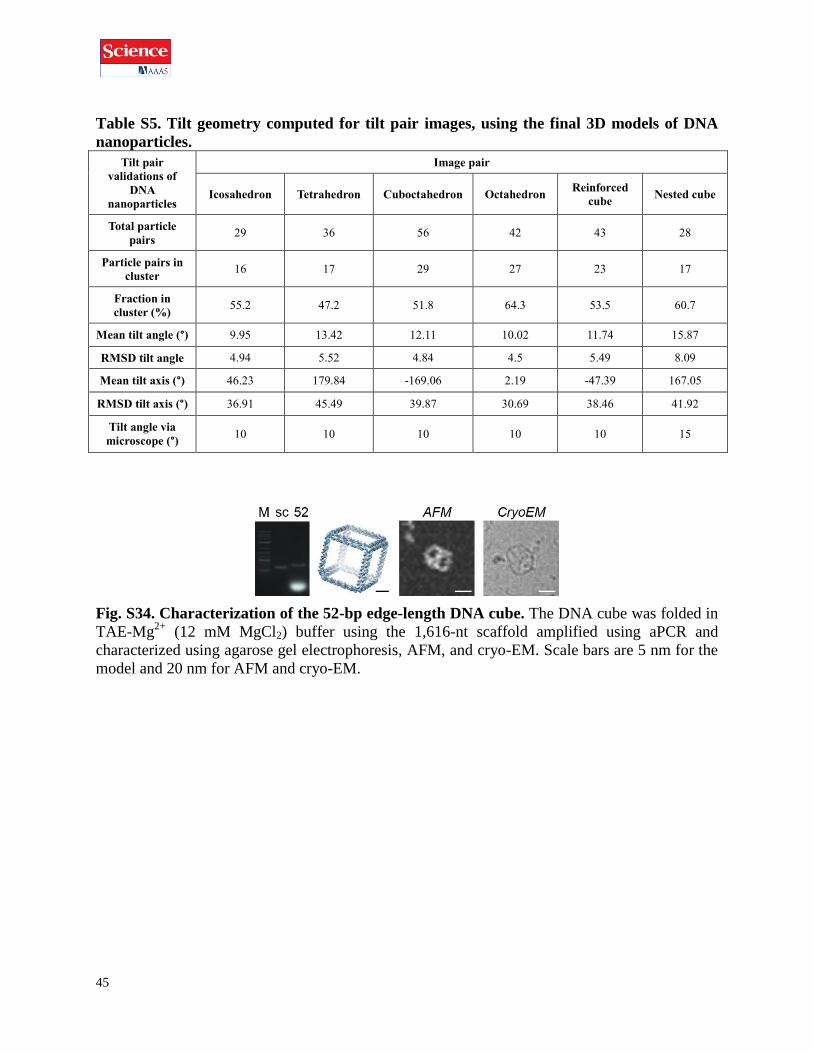
Fig. S34. Characterization of the 52-bp edge-length DNA cube. The DNA cube was folded in

TAE-Mg2+

(12 mM MgCl2) buffer using the 1,616-nt scaffold amplified using aPCR and

characterized using agarose gel electrophoresis, AFM, and cryo-EM. Scale bars are 5 nm for the

model and 20 nm for AFM and cryo-EM.

46

Fig. S35. AFM imaging of 52-bp edge-length DNA cube. Image size 2 μm × 2 μm.

Fig. S36. Cryo-EM imaging of 52-bp edge-length DNA cube.

47

S4 Effects of salt on folding of DNA nanostructures

This section contains the full AFM images of the inset presented in Fig. 6 to 7 for the 52-bp edge

length pentagonal bipyramid DNA origami and additional results obtained with tetrahedron 63-

bp edge length. In order to completely characterize the folding of our DNA nanostructures, TAE

buffers containing different MgCl2 concentration (in a range of 0 to 30 mM) or NaCl (in a range

of 0 mM to 2 M) were used to fold tetrahedron 63-bp edge length or pentagonal bipyramid 52-bp

edge length. The characterization was realized using agarose gel electrophoresis and AFM

imaging.

Folding of pentagonal bipyramid in increasing MgCl2 concentration

Fig. S37. AFM imaging of 52-bp edge-length DNA pentagonal bipyramid folded in 1 mM

MgCl2. Image size 2 μm × 2 μm.

48

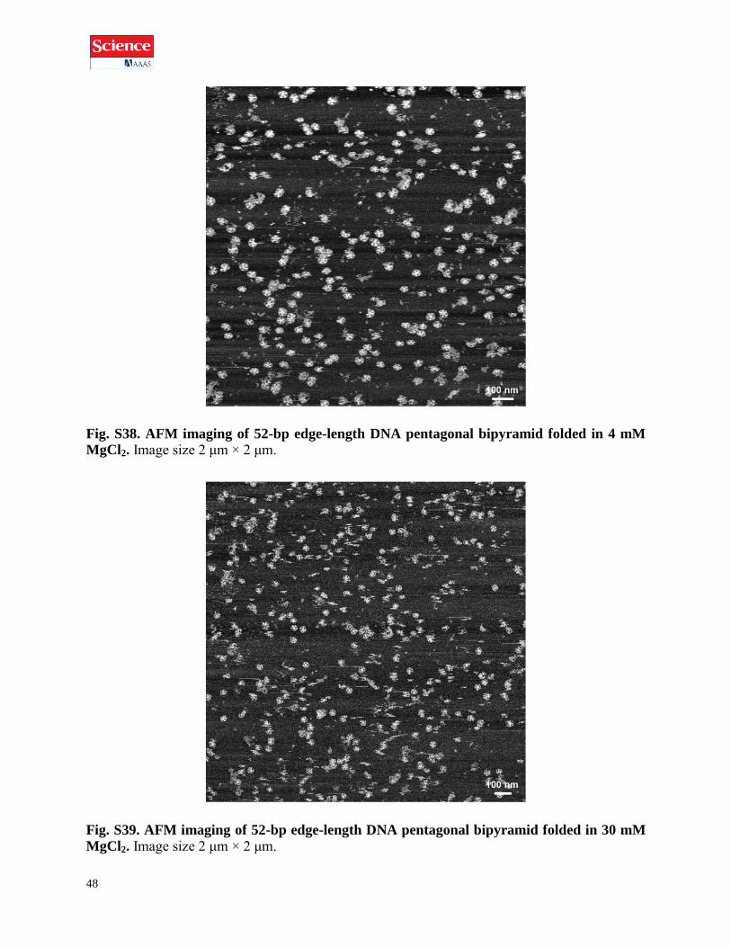
Fig. S38. AFM imaging of 52-bp edge-length DNA pentagonal bipyramid folded in 4 mM

MgCl2. Image size 2 μm × 2 μm.

Fig. S39. AFM imaging of 52-bp edge-length DNA pentagonal bipyramid folded in 30 mM

MgCl2. Image size 2 μm × 2 μm.

49

Folding of the DNA pentagonal bipyramid in increasing NaCl concentration

Fig. S40. AFM imaging of 52-bp edge-length DNA pentagonal bipyramid folded in 10 mM

NaCl. Image size 2 μm × 2 μm.

50

Fig. S41. AFM imaging of 52-bp edge-length DNA pentagonal bipyramid folded in 150 mM

NaCl. Image size 2 μm × 2 μm.

Fig. S42. AFM imaging of 52-bp edge-length DNA pentagonal bipyramid folded in 1 M

NaCl. Image size 2 μm × 2 μm.

51

Folding of the 63-bp edge-length tetrahedron in increasing concentration of MgCl2 and NaCl

Fig. S43. Folding of 63-bp edge-length DNA tetrahedron in buffer containing various

concentration of salt. The 63-bp edge-length DNA tetrahedron was folded in TRIS buffer with

increasing concentration of MgCl2 (0–30 mM) or increasing concentration of NaCl (0.01–2 M).

Folding was characterized with agarose gel electrophoresis and AFM imaging.

52

Fig. S44. AFM imaging of 63-bp edge-length DNA tetrahedron folded in 1 mM MgCl2. Image size 2 μm × 2 μm.

Fig. S45. AFM imaging of 63-bp edge-length DNA tetrahedron folded in 30 mM MgCl2. Image size 2 μm × 2 μm.

53

Fig. S46. AFM imaging of 63-bp edge-length DNA tetrahedron folded in 0.01 M NaCl. Image size 2 μm × 2 μm.

Fig. S47. AFM imaging of 63-bp edge-length DNA tetrahedron folded in 0.15 M NaCl.

Image size 2 μm × 2 μm.

54

Fig. S48. AFM imaging of 63-bp edge-length DNA tetrahedron folded in 1 M NaCl. Image

size 2 μm × 2 μm.

55

S5 Effects of buffer composition on folding of DNA origami objects

Fig. S49. Agarose gel of 52-bp edge-length DNA pentagonal bipyramid folded in PBS or

TAE buffer.

Fig. S50. AFM imaging of 52-bp edge-length DNA pentagonal bipyramid folded in PBS

buffer. Image size 2 μm × 2 μm.

56

Fig. S51. AFM imaging of 52-bp edge-length DNA pentagonal bipyramid folded in TAE

buffer. Image size 2 μm × 2 μm.

Fig. S52. AFM imaging of 52-bp edge-length DNA pentagonal bipyramid folded in TRIS-

NaCl 150 mM with phosphate (10 mM) and KCl (3 mM). Image size 2 μm × 2 μm.

57

Fig. S53. Agarose gel of 63-bp edge-length DNA tetrahedron folded in PBS or TAE buffer.

58

S6 Stability of DNA origami objects in physiological conditions

Fig. S54. AFM imaging of 52-bp edge-length DNA pentagonal bipyramid folded in TAE-

Mg2+

after buffer exchange with PBS. Image size 2 μm × 2 μm.

59

Fig. S55. AFM imaging of 52-bp edge-length DNA pentagonal bipyramid folded in TAE-

Mg2+

after buffer exchange with DMEM buffer. Image size 2 μm × 2 μm.

Fig. S56. AFM imaging of 52-bp edge-length DNA pentagonal bipyramid folded in TAE-

Mg2+

after buffer exchange with DMEM 2% dFBS. Image size 2 μm × 2 μm.

60

Fig. S57. AFM imaging of the 52-bp edge-length DNA pentagonal bipyramid folded in

TAE-Mg2+

after buffer exchange with DMEM 10% FBS. Image size 2 μm × 2 μm.

Fig. S58. Agarose gel electrophoresis of the 63-bp edge-length DNA tetrahedron to

determine its stability in DMEM with different concentrations of FBS for 6 hours.

61

Fig. S59. AFM imaging of 52-bp edge-length DNA pentagonal bipyramid folded in TAE-

Mg2+

after buffer exchange with TAE. Image size 2 μm × 2 μm.

62

Additional Tables (as a zipped archive):

Table S6. aPCR amplified sequences.

Table S7. Digested sequences.

Tables S8 to S27. Staple lists for the scaffolded DNA origami objects synthesized in this

paper.

Movies:

Movie S1. 3D rotation of icosahedron cryo-EM map with atomic model superimposed.

Movie S2. 3D rotation of tetrahedron cryo-EM map with atomic model superimposed.

Movie S3. 3D rotation of cuboctahedron cryo-EM map with atomic model superimposed.

Movie S4. 3D rotation of octahedron cryo-EM map with atomic model superimposed.

Movie S5. 3D rotation of reinforced cube cryo-EM map with atomic model superimposed.

Movie S6. 3D rotation of nested cube cryo-EM map with atomic model superimposed.

Movie S7. 3D rotation of octahedron cryo-EM map with alternate atomic model

superimposed. Before map-fitting. See Fig. S5(B), left.

References and Notes 1. N. C. Seeman, Nucleic acid junctions and lattices. J. Theor. Biol. 99, 237–247

(1982).doi:10.1016/0022-5193(82)90002-9 Medline

2. P. W. K. Rothemund, Folding DNA to create nanoscale shapes and patterns. Nature 440, 297–302 (2006).doi:10.1038/nature04586 Medline

3. Y. He, T. Ye, M. Su, C. Zhang, A. E. Ribbe, W. Jiang, C. Mao, Hierarchical self-assembly of DNA into symmetric supramolecular polyhedra. Nature 452, 198–201 (2008).doi:10.1038/nature06597 Medline

4. S. M. Douglas, H. Dietz, T. Liedl, B. Högberg, F. Graf, W. M. Shih, Self-assembly of DNA into nanoscale three-dimensional shapes. Nature 459, 414–418 (2009).doi:10.1038/nature08016 Medline

5. D. Han, S. Pal, J. Nangreave, Z. Deng, Y. Liu, H. Yan, DNA origami with complex curvatures in three-dimensional space. Science 332, 342–346 (2011).doi:10.1126/science.1202998 Medline

6. Y. Ke, L. L. Ong, W. M. Shih, P. Yin, Three-dimensional structures self-assembled from DNA bricks. Science 338, 1177–1183 (2012).doi:10.1126/science.1227268 Medline

7. M. R. Jones, N. C. Seeman, C. A. Mirkin, Nanomaterials. Programmable materials and the nature of the DNA bond. Science 347, 1260901 (2015).doi:10.1126/science.1260901 Medline

8. W. M. Shih, J. D. Quispe, G. F. Joyce, A 1.7-kilobase single-stranded DNA that folds into a nanoscale octahedron. Nature 427, 618–621 (2004).doi:10.1038/nature02307 Medline

9. C. E. Castro, F. Kilchherr, D.-N. Kim, E. L. Shiao, T. Wauer, P. Wortmann, M. Bathe, H. Dietz, A primer to scaffolded DNA origami. Nat. Methods 8, 221–229 (2011).doi:10.1038/nmeth.1570 Medline

10. H. Yan, S. H. Park, G. Finkelstein, J. H. Reif, T. H. LaBean, DNA-templated self-assembly of protein arrays and highly conductive nanowires. Science 301, 1882–1884 (2003).doi:10.1126/science.1089389 Medline

11. P. W. Rothemund, Scaffolded DNA origami: From generalized multicrossovers to polygonal networks, in Nanotechnology: Science and Computation (Springer, 2006), pp. 3–21.

12. F. Zhang, S. Jiang, S. Wu, Y. Li, C. Mao, Y. Liu, H. Yan, Complex wireframe DNA origami nanostructures with multi-arm junction vertices. Nat. Nanotechnol. 10, 779–784 (2015).doi:10.1038/nnano.2015.162 Medline

13. E. Benson, A. Mohammed, J. Gardell, S. Masich, E. Czeizler, P. Orponen, B. Högberg, DNA rendering of polyhedral meshes at the nanoscale. Nature 523, 441–444 (2015).doi:10.1038/nature14586 Medline

14. J. C. Sinclair, K. M. Davies, C. Vénien-Bryan, M. E. M. Noble, Generation of protein lattices by fusing proteins with matching rotational symmetry. Nat. Nanotechnol. 6, 558–562 (2011).doi:10.1038/nnano.2011.122 Medline

15. H. Gradišar, S. Božič, T. Doles, D. Vengust, I. Hafner-Bratkovič, A. Mertelj, B. Webb, A. Šali, S. Klavžar, R. Jerala, Design of a single-chain polypeptide tetrahedron assembled

63

from coiled-coil segments. Nat. Chem. Biol. 9, 362–366 (2013).doi:10.1038/nchembio.1248 Medline

16. S. M. Douglas, A. H. Marblestone, S. Teerapittayanon, A. Vazquez, G. M. Church, W. M. Shih, Rapid prototyping of 3D DNA-origami shapes with caDNAno. Nucleic Acids Res. 37, 5001–5006 (2009).doi:10.1093/nar/gkp436 Medline

17. D. Bhatia, S. Surana, S. Chakraborty, S. P. Koushika, Y. Krishnan, A synthetic icosahedral DNA-based host-cargo complex for functional in vivo imaging. Nat. Commun. 2, 339 (2011).doi:10.1038/ncomms1337 Medline

18. S. M. Douglas, I. Bachelet, G. M. Church, A logic-gated nanorobot for targeted transport of molecular payloads. Science 335, 831–834 (2012).doi:10.1126/science.1214081 Medline

19. A. Kuzyk, R. Schreiber, Z. Fan, G. Pardatscher, E.-M. Roller, A. Högele, F. C. Simmel, A. O. Govorov, T. Liedl, DNA-based self-assembly of chiral plasmonic nanostructures with tailored optical response. Nature 483, 311–314 (2012).doi:10.1038/nature10889 Medline

20. G. P. Acuna, F. M. Möller, P. Holzmeister, S. Beater, B. Lalkens, P. Tinnefeld, Fluorescence enhancement at docking sites of DNA-directed self-assembled nanoantennas. Science 338, 506–510 (2012).doi:10.1126/science.1228638 Medline

21. W. Sun, E. Boulais, Y. Hakobyan, W. L. Wang, A. Guan, M. Bathe, P. Yin, Casting inorganic structures with DNA molds. Science 346, 1258361 (2014).doi:10.1126/science.1258361 Medline

22. S. Helmi, C. Ziegler, D. J. Kauert, R. Seidel, Shape-controlled synthesis of gold nanostructures using DNA origami molds. Nano Lett. 14, 6693–6698 (2014).doi:10.1021/nl503441v Medline

23. V. Zhirnov, R. M. Zadegan, G. S. Sandhu, G. M. Church, W. L. Hughes, Nucleic acid memory. Nat. Mater. 15, 366–370 (2016).doi:10.1038/nmat4594 Medline

24. G. M. Church, Y. Gao, S. Kosuri, Next-generation digital information storage in DNA. Science 337, 1628–1628 (2012).doi:10.1126/science.1226355 Medline

25. N. Goldman, P. Bertone, S. Chen, C. Dessimoz, E. M. LeProust, B. Sipos, E. Birney, Towards practical, high-capacity, low-maintenance information storage in synthesized DNA. Nature 494, 77–80 (2013).doi:10.1038/nature11875 Medline

26. X. C. Bai, T. G. Martin, S. H. W. Scheres, H. Dietz, Cryo-EM structure of a 3D DNA-origami object. Proc. Natl. Acad. Sci. U.S.A. 109, 20012–20017 (2012).doi:10.1073/pnas.1215713109 Medline

27. Z. Wang, C. F. Hryc, B. Bammes, P. V. Afonine, J. Jakana, D.-H. Chen, X. Liu, M. L. Baker, C. Kao, S. J. Ludtke, M. F. Schmid, P. D. Adams, W. Chiu, An atomic model of brome mosaic virus using direct electron detection and real-space optimization. Nat. Commun. 5, 4808 (2014).doi:10.1038/ncomms5808 Medline

28. R. N. Irobalieva, J. M. Fogg, D. J. Catanese Jr., T. Sutthibutpong, M. Chen, A. K. Barker, S. J. Ludtke, S. A. Harris, M. F. Schmid, W. Chiu, L. Zechiedrich, Structural diversity of supercoiled DNA. Nat. Commun. 6, 8440 (2015).doi:10.1038/ncomms9440 Medline

64

29. Y. Krishnan, M. Bathe, Designer nucleic acids to probe and program the cell. Trends Cell Biol. 22, 624–633 (2012).doi:10.1016/j.tcb.2012.10.001 Medline

30. A. V. Pinheiro, D. Han, W. M. Shih, H. Yan, Challenges and opportunities for structural DNA nanotechnology. Nat. Nanotechnol. 6, 763–772 (2011).doi:10.1038/nnano.2011.187 Medline

31. T. J. Fu, N. C. Seeman, DNA double-crossover molecules. Biochemistry 32, 3211–3220 (1993).doi:10.1021/bi00064a003 Medline

32. See Supplementary Materials.

33. H. Dietz, S. M. Douglas, W. M. Shih, Folding DNA into twisted and curved nanoscale shapes. Science 325, 725–730 (2009).doi:10.1126/science.1174251 Medline

34. D.-N. Kim, F. Kilchherr, H. Dietz, M. Bathe, Quantitative prediction of 3D solution shape and flexibility of nucleic acid nanostructures. Nucleic Acids Res. 40, 2862–2868 (2012).doi:10.1093/nar/gkr1173 Medline

35. R. C. Prim, Shortest connection networks and some generalizations. Bell Syst. Tech. J. 36, 1389–1401 (1957). doi:10.1002/j.1538-7305.1957.tb01515.x

36. S. Pandey, M. Ewing, A. Kunas, N. Nguyen, D. H. Gracias, G. Menon, Algorithmic design of self-folding polyhedra. Proc. Natl. Acad. Sci. U.S.A. 108, 19885–19890 (2011).doi:10.1073/pnas.1110857108 Medline

37. S. W. Bent, U. Manber, On non-intersecting Eulerian circuits. Discrete Appl. Math. 18, 87–94 (1987). doi:10.1016/0166-218X(87)90045-X

38. Y. He, M. Su, P. A. Fang, C. Zhang, A. E. Ribbe, W. Jiang, C. Mao, On the chirality of self-assembled DNA octahedra. Angew. Chem. Int. Ed. Engl. 49, 748–751 (2010).doi:10.1002/anie.200904513 Medline

39. A. N. Marchi, I. Saaem, B. N. Vogen, S. Brown, T. H. LaBean, Toward larger DNA origami. Nano Lett. 14, 5740–5747 (2014).doi:10.1021/nl502626s Medline

40. C. I. Wooddell, R. R. Burgess, Use of asymmetric PCR to generate long primers and single-stranded DNA for incorporating cross-linking analogs into specific sites in a DNA probe. Genome Res. 6, 886–892 (1996).doi:10.1101/gr.6.9.886 Medline

41. K. E. Dunn, F. Dannenberg, T. E. Ouldridge, M. Kwiatkowska, A. J. Turberfield, J. Bath, Guiding the folding pathway of DNA origami. Nature 525, 82–86 (2015).doi:10.1038/nature14860 Medline

42. J.-P. J. Sobczak, T. G. Martin, T. Gerling, H. Dietz, Rapid folding of DNA into nanoscale shapes at constant temperature. Science 338, 1458–1461 (2012).doi:10.1126/science.1229919 Medline

43. H. Said, V. J. Schüller, F. J. Eber, C. Wege, T. Liedl, C. Richert, M1.3—a small scaffold for DNA origami. Nanoscale 5, 284–290 (2013).doi:10.1039/C2NR32393A Medline

44. T. Kato, R. P. Goodman, C. M. Erben, A. J. Turberfield, K. Namba, High-resolution structural analysis of a DNA nanostructure by cryoEM. Nano Lett. 9, 2747–2750 (2009).doi:10.1021/nl901265n Medline

65

45. Z. Liu, C. Tian, J. Yu, Y. Li, W. Jiang, C. Mao, Self-assembly of responsive multilayered DNA nanocages. J. Am. Chem. Soc. 137, 1730–1733 (2015).doi:10.1021/ja5101307 Medline

46. T. G. Martin, H. Dietz, Magnesium-free self-assembly of multi-layer DNA objects. Nat. Commun. 3, 1103 (2012).doi:10.1038/ncomms2095 Medline

47. N. C. Seeman, N. R. Kallenbach, Design of immobile nucleic acid junctions. Biophys. J. 44, 201–209 (1983).doi:10.1016/S0006-3495(83)84292-1 Medline

48. K. Pan, E. Boulais, L. Yang, M. Bathe, Structure-based model for light-harvesting properties of nucleic acid nanostructures. Nucleic Acids Res. 42, 2159–2170 (2014).doi:10.1093/nar/gkt1269 Medline

49. P. K. Dutta, R. Varghese, J. Nangreave, S. Lin, H. Yan, Y. Liu, DNA-directed artificial light-harvesting antenna. J. Am. Chem. Soc. 133, 11985–11993 (2011).doi:10.1021/ja1115138 Medline

50. W. Liu, M. Tagawa, H. L. Xin, T. Wang, H. Emamy, H. Li, K. G. Yager, F. W. Starr, A. V. Tkachenko, O. Gang, Diamond family of nanoparticle superlattices. Science 351, 582–586 (2016).doi:10.1126/science.aad2080 Medline

51. S. Surana, A. R. Shenoy, Y. Krishnan, Designing DNA nanodevices for compatibility with the immune system of higher organisms. Nat. Nanotechnol. 10, 741–747 (2015).doi:10.1038/nnano.2015.180 Medline

52. Y. Tian, Y. Zhang, T. Wang, H. L. Xin, H. Li, O. Gang, Lattice engineering through nanoparticle-DNA frameworks. Nat. Mater.; advance online publication (2016).doi:10.1038/nmat4571 Medline

53. G. Bellot, M. A. McClintock, C. Lin, W. M. Shih, Recovery of intact DNA nanostructures after agarose gel-based separation. Nat. Methods 8, 192–194 (2011).doi:10.1038/nmeth0311-192 Medline

54. G. Tang, L. Peng, P. R. Baldwin, D. S. Mann, W. Jiang, I. Rees, S. J. Ludtke, EMAN2: An extensible image processing suite for electron microscopy. J. Struct. Biol. 157, 38–46 (2007).doi:10.1016/j.jsb.2006.05.009 Medline

55. E. F. Pettersen, T. D. Goddard, C. C. Huang, G. S. Couch, D. M. Greenblatt, E. C. Meng, T. E. Ferrin, UCSF Chimera—a visualization system for exploratory research and analysis. J. Comput. Chem. 25, 1605–1612 (2004).doi:10.1002/jcc.20084 Medline

56. P. B. Rosenthal, R. Henderson, Optimal determination of particle orientation, absolute hand, and contrast loss in single-particle electron cryomicroscopy. J. Mol. Biol. 333, 721–745 (2003).doi:10.1016/j.jmb.2003.07.013 Medline

57. J. A. Ellis-Monaghan, A. McDowell, I. Moffatt, G. Pangborn, DNA origami and the complexity of Eulerian circuits with turning costs. Nat. Comput. 14, 1–13 (2014).

58. N. R. Kallenbach, R.-I. Ma, N. C. Seeman, An immobile nucleic acid junction constructed from oligonucleotides. Nature 305, 829–831 (1983). doi:10.1038/305829a0

66

59. K. Pan, D.-N. Kim, F. Zhang, M. R. Adendorff, H. Yan, M. Bathe, Lattice-free prediction of three-dimensional structure of programmed DNA assemblies. Nat. Commun. 5, 5578 (2014).doi:10.1038/ncomms6578 Medline

60. A. Untergasser, I. Cutcutache, T. Koressaar, J. Ye, B. C. Faircloth, M. Remm, S. G. Rozen, Primer3—new capabilities and interfaces. Nucleic Acids Res. 40, e115–e115 (2012).doi:10.1093/nar/gks596 Medline

61. T. Koressaar, M. Remm, Enhancements and modifications of primer design program Primer3. Bioinformatics 23, 1289–1291 (2007).doi:10.1093/bioinformatics/btm091 Medline

62. Q. Mei, X. Wei, F. Su, Y. Liu, C. Youngbull, R. Johnson, S. Lindsay, H. Yan, D. Meldrum, Stability of DNA origami nanoarrays in cell lysate. Nano Lett. 11, 1477–1482 (2011).doi:10.1021/nl1040836 Medline

63. R. Henderson, S. Chen, J. Z. Chen, N. Grigorieff, L. A. Passmore, L. Ciccarelli, J. L. Rubinstein, R. A. Crowther, P. L. Stewart, P. B. Rosenthal, Tilt-pair analysis of images from a range of different specimens in single-particle electron cryomicroscopy. J. Mol. Biol. 413, 1028–1046 (2011).doi:10.1016/j.jmb.2011.09.008 Medline

64. S. C. Murray, J. Flanagan, O. B. Popova, W. Chiu, S. J. Ludtke, I. I. Serysheva, Validation of cryo-EM structure of IP₃R1 channel. Structure 21, 900–909 (2013).doi:10.1016/j.str.2013.04.016 Medline

67