1

Supplementary Figures

Supplementary Figure 1 | Materials and equipment for production of LIG from PI by laser

scribing. a, Photographs of commercial Kapton PI sheets (left) with a 30 cm ruler, and the laser

cutting system (right). b and c, Photographs of an owl and a letter R patterned on PI substrates;

scale bar, 5 mm. In b and c, black contrast is LIG after exposure to the laser, while the lighter

background corresponds to PI. The laser power used to scribe the images was 3.6 W.

2

Supplementary Figure 2 | Raman spectra of control samples. PI sheets were carbonized in a

furnace under Ar flow of 300 sccm for 3 h with annealing temperatures: 800 °C, 1000 °C and

1500 °C. Raman spectra show that these carbonized materials were glassy and amorphous carbon.

3

Supplementary Figure 3 | XPS characterization of LIG-3.6 W films. a, XPS surveys of LIG

and PI. Comparasion curves show that the oxygen and nitrogen peaks were significantly

suppressed after PI was converted to LIG. b, High resolution C1s XPS spectrum of the LIG film

and PI, showing the dominant C—C peak. The C—N, C—O and C=O peaks from PI were

greatly reduced in the C1s XPS spectrum of LIG, which indicates that LIG was primarily sp2-

carbons. c, High resolution O1s XPS spectrum of a LIG-3.6 W film and PI. After laser

conversion, the C—O (533.2 eV) peak becomes more dominant than C=O (531.8 eV). d, High

resolution N1s XPS spectrum of a LIG-3.6 W film and PI. The intensity of the N1s peak was

greatly reduced after laser exposure.

4

Supplementary Figure 4 | FTIR spectra of LIG-3.6 W and PI films. FTIR spectra of PI

showing distinct peaks at 1090-1776 cm-1

, corresponding to the well-defined stretching and

bending modes of the C—O, C—N, and C=C bonds. After the laser scribing, a broad absorption

from 1000 cm-1

to 1700 cm-1

shows that the laser scribing leads to a large variation in the local

environment.

5

Supplementary Figure 5 | TEM characterization of LIG-3.6 W flakes. a, TEM image of a

thin LIG flake atop a carbon grid; scale bar, 200 nm. b, TEM image of a thick LIG flake showing

entangled tree-like ripples; scale bar, 100 nm. Inset is the HRTEM image of the yellow-circled

region showing the mesoporous structures; scale bar, 5 nm. c and d, TEM images of LIG in

bright and dark field view; scale bars, 10 nm. In dark field view, folded graphene containing

several pores between 5 to 10 nm can be seen. These pores indicated in orange arrows in d result

from curvature of the graphene layers induced by abundant pentagon-heptagon pairs1.

6

Supplementary Figure 6 | TEM characterization of LIG-3.6 W flakes using filtering

techniques. a, The bright-field TEM image of the studied area; scale bar, 5 nm. b, FFT of the

7

LIG sample. The area has two distinct parts that can be seen on the indexed diffractogram FFT

with the hexagonal crystal structure of carbon with lattice parameters a = 2.461 Å and c = 6.708

Å. The outer circle spots are reflections of the type (10.0) or (1.-1.0), corresponding to the basal

plane of graphite 00.1. The layers are, however, very disordered and produce a rotational pattern

with d-spacing of 2.10 Å. The inner circle spots are type (00.2) corresponding to a d-spacing of

3.35 Å of the folded layers of graphene containing the cavities. c, The filter uses the inner circle

of type (00.2) spots and neglects the outer circle of type (10.0) spots. d, Corresponding filtered

image from c; scale bar, 5 nm. The folded graphene structure was enhanced. e, The filter uses the

outer circle of type (10.0) spots and neglects the inner circle of type (00.2) spots. f,

Corresponding filtered image from e; scale bar, 5 nm. The disordered graphene structure was

enhanced.

8

Supplementary Figure 7 | BET specific surface area of LIG-3.6 W. The surface area of this

sample was ~342 m2·g

-1. Pore sizes are distributed at 2.36 nm, 3.68 nm, 5.37 nm and 8.94 nm.

9

Supplementary Figure 8 | TGA characterizations of LIG-3.6 W, PI and graphene oxide

(GO) in argon. Compared to GO, which significantly decomposes at ~ 190 °C, LIG is stable at >

900 °C. PI starts to decompose at 550 °C.

10

Supplementary Figure 9 | Correlation of threshold laser power to scan rate. The

threshold power shows a linear dependence on the scan rate. Conditions indicated by the

shaded area lead to laser graphitization.

11

Supplementary Figure 10 | Characterizations of backsides of LIG films. a, Scheme of the

backsides of LIG films peeled from PI substrates. b, c, d, SEM images of backsides of LIG films

obtained at laser powers of b 2.4 W; c, 3.6 W; and d, 4.8 W. All of the scale bars are 10 µm. The

images show increased pore size as the laser power was increased.

12

Supplementary Figure 11 | Characterization of LIG from different polymers. a, A

photograph of patterns induced by lasers on different polymers (PI, PEI and PET) at laser power

of 3.0 W. Note that the only two polymers that blackened in this way were PI and PEI. b, Raman

spectrum of PEI-derived LIG obtained with a laser power of 3.0 W.

13

Supplementary Figure 12 | Electrochemical characterizations of LIG-MSCs obtained from

PI and PEI using different laser powers in 1 M H2SO4. a, Comparison of CV curves of LIG-

MSCs obtained from PI at scan rates of 100 mV·s-1

. b, Specific areal capacitances of LIG-MSCs

obtained from PI, calculated from CC curves at current densities of 0.2 mA·cm-2

, as a function of

the laser power. c, Comparison of CV curves of LIG-MSCs obtained from PEI at scan rates of 1

V·s-1

. d, Specific areal capacitances of LIG-MSCs obtained from PEI, calculated from CC curves

at a current density of 0.2 mA·cm-2

, as a function of the laser power. Compared to PEI derived

LIG-MSCs, LIG-MSCs obtained from PI have ~10 × higher capacitances prepared at the same

laser powers.

14

Supplementary Figure 13 | Impedance spectroscopy of LIG-MSCs obtained from PI using

a laser power of 4.8 W in 1 M H2SO4. Equivalent series resistance is as low as 7 Ω obtained at

a high frequency range.

15

Supplementary Figure 14 | Electrochemical characterizations of LIG-MSCs obtained with

laser power of 4.8 W in BMIM-BF4. a and b, CV curves of LIG-MSCs at scan rates from 20

mV·s-1

to 5 V·s-1

. c, Specific areal capacitances vs. scan rates. d and e, CC curves of LIG-MSCs

at discharge current densities from 0.1 mA·cm-2

to 7 mA·cm-2

. The voltage drop is shown

graphically in e. f, Specific areal capacitances vs. discharge current densities.

16

Supplementary Figure 15 | Comparison volumetric capacitances, calculated from CC

curves, of LIG-MSCs in aqueous electrolyte and ionic liquid (IL). a, Specific volumetric

capacitances as a function of discharge current densities in 1 M H2SO4. b, Specific volumetric

capacitances as a function of discharge current densities in BMIM-BF4.

17

Supplementary Figure 16 | Electrochemical performance of LIG-MSCs in series/parallel

combinations. Electrolyte for devices in a and b is 1 M H2SO4, and for devices in c it is BMIM-

BF4. a, CC curves of two tandem LIG-MSCs connected in series with the same discharge current

density of 1 mA·cm-2

. The operation potential window is doubled in serial configuration. b, CC

curves of two tandem LIG-MSCs in parallel assembly with the same discharge current density of

1 mA·cm-2

. In this configuration capacitance is almost doubled. c, CC curves of single LIG-

MSCs and 10 parallel LIG-MSCs at discharge current densities of 1 mA·cm-2

and 10 mA·cm-2

,

respectively. Current density increases by a factor of 10 with 10 parallel single devices. Inset is a

lighted LED powered by 10 parallel LIG-MSCs.

18

Supplementary Figure 17 | Comparison Ragone plots of different energy storage devices. a,

Specific volumetric energy and power densities of energy storage devices. b, Specific areal

energy and power densities of LIG-MSCs and LSG-MSCs. Data were reproduced from

refences2,3

.

19

Supplementary Figure 18 | Capacity retention of LIG-MSCs constructed with LIG-4.8 W

in 1 M H2SO4 and ionic liquid (BMIM-BF4). a, Capacitance, calculated from CV curves at a

scan rate of 100 mV·s-1

, increases to 114% of the original value after 2750 cycles, and then

retains almost the same value after 9000 cycles. b, Capacitance, calculated from CV curves at a

scan rate of 100 mV·s-1

. The capacitance degrades to 95.5% of original value after 1000 cycles,

and then stabilizes at 93.5% after 7000 cycles.

20

Supplementary Figure 19 | CV curves of LIG-MSCs obtained with laser power of 4.8 W in

1M H2SO4 (a) and BMIM-BF4 (b). The curves were obtained at a sweep rate of 100 mV·s-1

after every 1000 cycles.

21

Supplementary Figure 20 | Atomic structure of the calculated polycrystalline graphene

sheets. The arrows indicate the unit cell, and the grain boundary regions are shaded. Numbers

show two types of misorientation angles (21.8° and 32.2°) between grains.

22

Supplementary Tables

Materials Carbon (%) Oxygen (%) Nitrogen (%)

Polyimide 70.5 22.5 7.0

LIG-1.2 W 72.2 20.3 7.5

LIG-1.8 W 74.7 18.2 7.1

LIG-2.4 W 97.3 2.5 0.2

LIG-3.0 W 95.5 4.1 0.4

LIG-3.6 W 94.5 4.9 0.6

LIG-4.2 W 94.0 5.5 0.5

LIG-4.8 W 92.3 6.9 0.8

LIG-5.4 W 91.3 7.7 1.0

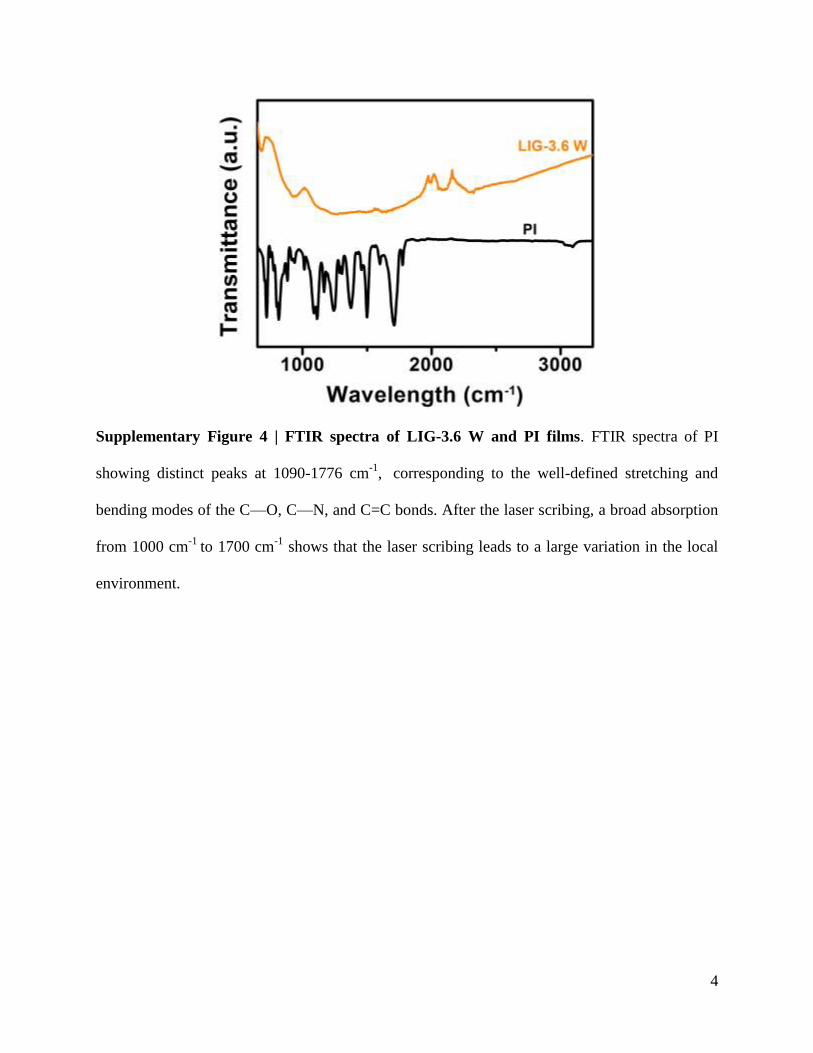
Supplementary Table 1| Summary of atomic percentage of elements in raw material (PI)

and LIG derived from different laser powers. All of the data was obtained by high-resolution

XPS scans.

23

Supplementary Table 2 | Summary of polymers, their chemical repeat units and their LIG-

forming capability. Out of 15 polymers, only PI and PEI were successfully converted to

LIG. Nonaromatic hydrocarbons undergo almost complete degradation without graphitization.

Formation of LIG from poly- or heterocyclic structures such as the imide group in PI and PEI

polymers favor LIG formation. PAN films are not commercially available and were thus

prepared in-house. Though PAN is a precursor to carbon fiber, it does not graphitize well unless

heated slowly to permit cyclization and N-extrusion.

24

Supplementary References

1. Ma, J., Alfe, D., Michaelides, A. & Wang, E. Stone-Wales defects in graphene and other

planar sp(2)-bonded materials. Phys. Rev. B 80 (2009).

2. El-Kady, M. F. & Kaner, R. B. Scalable fabrication of high-power graphene micro-

supercapacitors for flexible and on-chip energy storage. Nat. Commun. 4, 1475 (2013).

3. Wu, Z. S., Parvez, K., Feng, X. L. & Mullen, K. Graphene-based in-plane micro-

supercapacitors with high power and energy densities. Nat. Commun. 4, 2487 (2013).