Supplementary budget estimates 2011-2012

Senate Rural Affairs and Transport Legislation Committee ANSWERS TO QUESTIONS ON NOTICE

Supplementary Budget Estimates October 2011 Agriculture, Fisheries and Forestry

Question: 31 Division/Agency: ABARES – Australian Bureau of Agricultural and Resource Economics and Sciences Topic: Climate change - modelling Proof Hansard page: 47 Senator CORMANN asked: Senator CORMANN: The reason being that Treasury told a committee of the Senate as late as 23 September that it was a matter for ABARES as to whether and to what extent the GTEM model would be released. Between 2000, when you first released the Global Trade Environment Model (GTEM) for public use, and 2007, when you released an updated version, expecting to release further updates to the code and so on over the following months, what sorts of refinements took place in the period 2000 to 2007 and did any of those refinements involve Treasury in any way, shape or form? Dr Sheales: I would have to take that on notice. I am not sure of the details. It was not in my area of responsibility and I am just not sure of the details. Senator CORMANN asked: Mr Glyde: Between 2000 and 2007 there would have been quite a bit of updating of data sets for particular jobs that we might have done. We would be better off taking it on notice and being precise about what happened and for what purpose. Answer: Between 2000 and 2007 a number of key developments were made to the GTEM model code and database by ABARES. All refinements during this period were made without Treasury involvement. Key developments and refinements during this time included: 1. Changes to the model code

• Adding a ‘learning by doing function’ which reflects the decrease in costs of new clean technologies that come with experience.

• Adding a ‘resource extraction function’ to account for the increasing cost of extracting natural resources that have been heavily mined.

• Introducing a new form of the ‘emissions response functions’ to better reflect the emissions abatement opportunities under a carbon price.

• Allowing households to substitute between different types of fuels. • Changing the modelling of substitution between electricity technologies to reflect

differences in uptake between technologies. • Introducing a new modelling methodology for labour supply and participation rates. • Expanding the emissions accounting framework to include new sectors and

greenhouse gases, including waste emissions.



Question: 31 (continued) 2. Updates to the database

• Updating the base year to 2001, including industry cost structures, in accordance with the Global Trade Analysis Project version 6.1.

• Updating energy and emissions data to 2001. • Expanding the number of sectors (mainly renewable energy sectors and carbon

capture and storage). • Updating population data to 2001 using United Nations sources.

3. Changes to model assumptions for the reference case

• Updating the economic, population and energy efficiency assumptions based on new information.

• Updating the electricity generation technology shares to 2050. • Incorporating expected emissions abatement opportunities.

Most of these amendments have been documented in the latest version of the GTEM documentation (Pant 2007). Pant, H 2007, GTEM: the Global Trade and Environment Model, ABARES, Canberra.



Question: 33 Division/Agency: ABARES – Australian Bureau of Agricultural and Resource Economics and Sciences Topic: Climate change – modelling Proof Hansard page: 51/52 Senator BOSWELL asked: Senator BOSWELL: Mr Glyde, I want to refer to the evidence you gave before lunch in which you said that there was a meeting between Treasury and ABARES about the public release of the GTEM model. What dates were those meetings held and who was at the meetings? Mr Glyde: Senator Cormann asked this question right at the start of this afternoon's proceedings. Senator BOSWELL: What was the answer? Mr Glyde: My recollection was that we thought that the timing of it was around late August, early September but we would have to take on notice the precise timing. We also observed that it was not just meetings; there were also telephone calls and email traffic on this matter. Senator BOSWELL: Were Dr Gruen and Ms Quinn at the meeting? Mr Glyde: I would have to take that on notice. I was not involved in the meeting. Dr Sheales: Both have been involved at different points in discussions. Answer: There were a series of discussions and email exchanges between ABARES and The Treasury during September and October 2011 regarding the public release of the Global Trade and Environment Model. In addition to other phone calls and emails, the following teleconferences occurred: • 6 September 2011 a teleconference between Ms Meghan Quinn and Dr Liangyue Cao of

Treasury and Dr Sheales and Dr Ahammad of ABARES • 6 October 2011 a teleconference between Dr Gruen, Ben Dolman and Dr Liangyue Cao

of Treasury and Dr Sheales and Dr Ahammad.



Question: 34 Division/Agency: ABARES - Australian Bureau of Agricultural and Resource Economics and Sciences Topic: Exceptional circumstances Proof Hansard page: 52/53 Senator BOSWELL asked:

Dr Sheales: That is not a problem. Answer: Please refer to the answer to Question 33 from the Supplementary Budget Estimates hearing on 17 October 2011.

Senator WILLIAMS: In relation to the exceptional circumstances application for Delungra, they did not meet the criteria of having a severe downturn in their income. Did ABARES do a report for that application? Dr Sheales: Yes, as far as I know, we did. Do not ask me the details because I do not have them with me! Senator WILLIAMS: I was just amazed, because they made the 0.5 percentile. It must be a severe downturn in income. We had three accountants come forward showing the figures of the severe reduction in income as well as two businesses. Did you see that second application by those accountants? Dr Ritman: Apparently, yes, we did do a report. It was made publicly available. Senator WILLIAMS: Yes, but after you did your report we put another application in on the grounds that we had three accounting firms backing up the downturn in income plus two of the small business men of the Delungra-Warialda area. Did you see that second application where we forwarded the accountants' figures? Mr McDonald: The information you refer to is in letters of support from accountants. They followed the government's decision on the original application from the New South Wales government. Senator WILLIAMS: Are you sure there wasn't a second case where they actually provided figures after the first rejection? I believe there was. Mr McDonald: I am aware of the letters of support from the accountants Senator WILLIAMS: But you are not aware of further information put forward by accountants giving figures of the downturn in that district, and from businesses as well? Mr McDonald: I cannot comment on further information beyond the letters of support provided by the accountants that I believe was forwarded by you and another senator. Senator BOSWELL: Dr Sheales, you mentioned the meeting in late August or early September. Can you tell us on notice who was at that meeting, please?



Question: 69 Division/Agency: ABARES – Australian Bureau of Agricultural and Resource Economics and Sciences Topic: Aerial survey Proof Hansard page: 123 Senator COLBECK asked:

Senator COLBECK: That would be great, thanks. Answer: The scientific aerial survey paper is attached as requested at Attachment 1.

Senator COLBECK: No. You said it was the second highest on record. So when was the previous high? Dr Begg: 1993. Senator COLBECK: That document was held prior to this process. When will that be published? Dr Begg: Now that the commission meeting is over, all those papers can be provided. We can get you a copy of that.

CCSBT-ESC/1107/15

The aerial survey index of abundance: updated analysis

methods and results for the 2010/11 fishing season

Paige Eveson

Jessica Farley

Mark Bravington

Prepared for the CCSBT Extended Scientific Committee for the 16th Meeting of the

Scientific Committee 19-28 July 2011

Bali, Indonesia

Question: 69 (continued) Attachment 1

pinto carmen

Typewritten Text

pinto carmen

Typewritten Text

pinto carmen

Typewritten Text

pinto carmen

Typewritten Text

pinto carmen

Typewritten Text

pinto carmen

Typewritten Text

pinto carmen

Typewritten Text

pinto carmen

Typewritten Text

pinto carmen

Typewritten Text

CCSBT-ESC/1107/15

Table of Contents

Abstract ......................................................................................................................................1

Introduction................................................................................................................................1

Field procedures.........................................................................................................................2

Data preparation.........................................................................................................................3

Search effort and SBT sightings ................................................................................................4

Environmental variables ............................................................................................................8

Methods of analysis .................................................................................................................10

Results......................................................................................................................................12

Summary ..................................................................................................................................14

References................................................................................................................................14

Acknowledgements..................................................................................................................15

Appendix A – Methods of analysis..........................................................................................16

Biomass per sighting (BpS) model .......................................................................................17

Sightings per mile (SpM) model ..........................................................................................17

Combined analysis................................................................................................................19

Appendix B – CV calculations ................................................................................................20

Appendix C: Results and diagnostics .....................................................................................23

Biomass per sighting (BpS) model .......................................................................................23

Sightings per mile (SpM) model ..........................................................................................27


CCSBT-ESC/1107/15

1

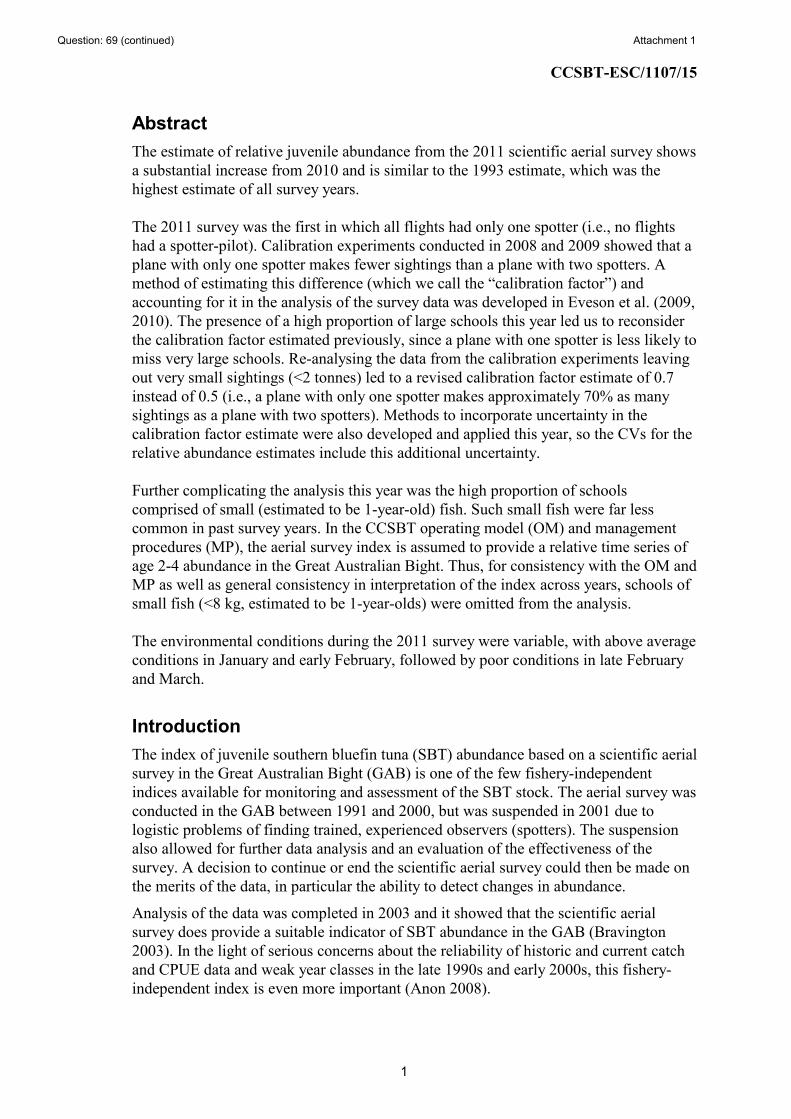
Abstract

The estimate of relative juvenile abundance from the 2011 scientific aerial survey shows

a substantial increase from 2010 and is similar to the 1993 estimate, which was the

highest estimate of all survey years.

The 2011 survey was the first in which all flights had only one spotter (i.e., no flights

had a spotter-pilot). Calibration experiments conducted in 2008 and 2009 showed that a

plane with only one spotter makes fewer sightings than a plane with two spotters. A

method of estimating this difference (which we call the “calibration factor”) and

accounting for it in the analysis of the survey data was developed in Eveson et al. (2009,

2010). The presence of a high proportion of large schools this year led us to reconsider

the calibration factor estimated previously, since a plane with one spotter is less likely to

miss very large schools. Re-analysing the data from the calibration experiments leaving

out very small sightings (<2 tonnes) led to a revised calibration factor estimate of 0.7

instead of 0.5 (i.e., a plane with only one spotter makes approximately 70% as many

sightings as a plane with two spotters). Methods to incorporate uncertainty in the

calibration factor estimate were also developed and applied this year, so the CVs for the

relative abundance estimates include this additional uncertainty.

Further complicating the analysis this year was the high proportion of schools

comprised of small (estimated to be 1-year-old) fish. Such small fish were far less

common in past survey years. In the CCSBT operating model (OM) and management

procedures (MP), the aerial survey index is assumed to provide a relative time series of

age 2-4 abundance in the Great Australian Bight. Thus, for consistency with the OM and

MP as well as general consistency in interpretation of the index across years, schools of

small fish (<8 kg, estimated to be 1-year-olds) were omitted from the analysis.

The environmental conditions during the 2011 survey were variable, with above average

conditions in January and early February, followed by poor conditions in late February

and March.

Introduction

The index of juvenile southern bluefin tuna (SBT) abundance based on a scientific aerial

survey in the Great Australian Bight (GAB) is one of the few fishery-independent

indices available for monitoring and assessment of the SBT stock. The aerial survey was

conducted in the GAB between 1991 and 2000, but was suspended in 2001 due to

logistic problems of finding trained, experienced observers (spotters). The suspension

also allowed for further data analysis and an evaluation of the effectiveness of the

survey. A decision to continue or end the scientific aerial survey could then be made on

the merits of the data, in particular the ability to detect changes in abundance.

Analysis of the data was completed in 2003 and it showed that the scientific aerial

survey does provide a suitable indicator of SBT abundance in the GAB (Bravington

2003). In the light of serious concerns about the reliability of historic and current catch

and CPUE data and weak year classes in the late 1990s and early 2000s, this fishery-

independent index is even more important (Anon 2008).


CCSBT-ESC/1107/15

2

In 2005, the full scientific line-transect aerial survey was re-established in the GAB, and

this survey has been conducted each year since. New analysis methods were developed

and have subsequently been refined. Based on these methods, an index of abundance

across all survey years has been constructed.

In addition, in 2007 a large-scale calibration experiment was initiated with the primary

purpose of comparing SBT sighting rates by one observer versus two observers in a

plane. This was done in light of the fact that future surveys would have only one

observer in a plane (as was the case for one of the two planes flying in the 2010 survey

and both planes flying in the 2011 survey). The data provided useful information about

differences in sightings between observers (e.g., sightings made by one observer are

often missed by another observer). However, it proved difficult to definitively estimate

the effect of the number of observers on the index.

In 2008 and 2009 a new calibration experiment was designed and run in parallel with

the full scientific aerial survey. This calibration experiment was designed to compare:

• the number of SBT sightings;

• and total estimated biomass of SBT observed;

by the single observer plane versus the survey plane (with two observers) over the same

area and time strata.

This report summarises the field procedures and data collected during the 2011 season,

which was the first season that both survey planes had only one observer. A method for

accounting for the fact that a plane with one observer makes fewer sightings than a

plane with two observers was developed in Eveson et al. (2009, 2010) based on data

from the calibration experiments. These methods were refined this year and applied in

the analysis. A couple of small additional changes were made to the analysis methods

this year, including a change to the way in which the observer effect is included in the

sightings model (as discussed in Appendix A), and the omission of schools of 1-year-

old fish from the analysis (as discussed in the Data preparation section). The current

methods for analysing the data are described, and results are presented from applying

these methods to the data from all survey years.

Field procedures

The 2011 scientific aerial survey was conducted in the GAB between 1 January and 31

March 2011. As for previous surveys (e.g. Eveson et al. 2009; 2010), two Rockwell

Aero Commander 500S were chartered for the season - one for the full three months

(plane 1) and a second for January and February only (plane 2). Each plane contained

one observer and a non-spotting pilot. The same observers employed for the 2007 to

2010 surveys were used in the 2011 survey. In addition, a spotter-pilot used in the 1993-

1998 and 2008-10 surveys was used as an observer in one of the planes in January.

The survey followed the protocols established for the 2000 survey (Cowling 2000) and

used in all subsequent surveys with respect to the area searched, plane flying height and

speed, minimum environmental conditions, time of day the survey lines were flown, and

data recording protocols. Fifteen north-south transect lines (Figure 1) were surveyed. A

complete replicate of the GAB consists of a subset of 12 (of the 15) lines divided into 4


CCSBT-ESC/1107/15

3

blocks. The remaining 3 lines in a replicate (either: 1, 3 and 14, or 2, 13 and 15) were

not searched, as SBT abundance is historically low in these areas and surveying a subset

increases the number of complete replicate of the GAB in the survey.

When flying along a line, the single observer searched the sea surface for patches of

SBT from his side of the plane (the right side) through 180° to the other side of the

plane (the left side). When both planes were surveying, they always surveyed

neighbouring blocks. The blocks were chosen with the aim of allowing both planes to

complete each block at least once per replicate. When conditions allowed for only one

plane to survey (e.g. only one block was suitable), then preference was given to plane

with the observer that had not surveyed that block.

The 2011 field operation was successful, largely due to the above average weather

conditions in January and early February, and the availability of two planes at that time.

The weather in late February and March was particularly windy, cloudy and wet.

Despite this, almost 7 replicates of the GAB were completed in 2011, which is similar

to 2010 but higher than the 3-5 replicates for the preceding 5 years. The total flying time

(transit and transect time) for the 2011 survey was 204.8 hours, compared to 213.6

hours in 2010.

Figure 1. Location of the 15 north-south transect lines for the scientific aerial survey in

the GAB.

Nullarbor

36°S

34°S

32°S

Ceduna

Port Lincoln

128°E 130°E 132°E 134°E 136°E

+

+

+

1 2 3 4 5 6 78

9

10

11

1213

1514

Data preparation

The data collected from the 2011 survey were loaded into the aerial survey database and

checked for any obvious errors or inconsistencies and corrections made as necessary. In

order for the analyses to be comparable between all survey years, only data collected in

a similar manner from a common area were included in the data summaries and analyses

presented in this report. In particular, only search effort and sightings made along

north/south transect lines in the unextended (pre-1999) survey area and sightings made


CCSBT-ESC/1107/15

4

within 6 nm of a transect line were included (see Basson et al. 2005 for details). In cases

where a sighting consisted of more than one school, then the sighting was included if at

least one of the schools was within 6 nm of the line. We excluded secondary sightings

and any search distance and sightings made during the aborted section of a transect line

(see Eveson et al. 2006 for details).

This year’s data included a high proportion of schools of small (1-year-old) fish, which

was unusual compared to past survey years. The percent of the total tonnage of SBT

spotted that was estimated to be fish less than 8 kg was 30.8% in 2011. The next highest

was 16.1% in 2010, followed by 13.2% in 2009, and ranging from 0.6 to 8.8% in other

years (Table 1). Because the spotters estimate average weight, not age, of fish in

schools, we use 8 kg as an average weight cut-off between 1-year-olds and 2-year-olds.

An 8 kg cut-off was used because it equates to a length of 73 cm using the weight-

length relationship of Robins (1963), and a 73 cm fish is a reasonable estimate of the

upper limit of a 1 year old fish (and lower limit of a 2 year old fish) based on both the

GAB direct age data (Farley et al., 2011) and the CCSBT growth curve (Eveson, 2011).

When two spotters are in a plane, they both make independent estimates of the size of

fish in each school, so we averaged their estimates to come up with a single estimate of

average fish size. Although early validation experiments found that spotters’ estimates

of average fish size within a school could be inconsistent (Cowling et al. 2002), we are

fairly confident based on conversations with the spotters that they can distinguish

schools of very small (1-year-old) fish from schools of larger/older fish.

In the CCSBT operating model (OM) and management procedures (MP), the aerial

survey index is assumed to provide a relative time series of age 2-4 abundance in the

Great Australian Bight. Thus, for consistency with the OM and MP as well as general

consistency in interpretation of the index across years, schools estimated to be

comprised of 1-year-old fish (i.e., that had an average fish size estimate of less than

8 kg) were omitted from the analysis.

Search effort and SBT sightings

A summary of the total search effort and SBT sightings made in each survey year is

given in Table 1. All of the values are based on raw data, which have not been corrected

for environmental factors or observer effects. This table, and all summary information

and results presented in this report, include only the data outlined in the previous section

as being appropriate for analysis. Recall the change this year, in that we are omitting

schools comprised of fish less than <8 kg on average. This has the biggest effect on the

current year, but affects all years to some degree. Also note that the summary statistics

for 2010 include data from all flights, some of which had only one observer; for 2011,

all data comes from flights with only one observer.

The total distance searched in 2011 was similar to last year, which was the greatest since

1996. This was due to having two planes available to fly during the first half of the

survey when weather conditions were favourable. The raw sightings rate (number of

sightings per 100 nm) was about average, but the biomass per nm was highest of all

survey years due to a lot of large patches (Table 1, Figure 2). However, it is important to

remember that the statistics for 2010 and 2011 include data from flights with only one


CCSBT-ESC/1107/15

5

observer, so caution must be used in comparing them to previous years (which is why

we have chosen not to include the figure with the raw sightings rate and biomass per nm

plotted against year).

Similar to last year, sightings in 2011 were concentrated in the eastern half of the survey

area, with the greatest concentration along the shelf-break (Figure 3). The data this year

continues to support that there has been a general eastward shift in the distribution of

SBT sightings over the years.

Table 1. Summary of aerial survey data by survey year. Only data considered suitable for

analysis (as outlined in text) are included. All biomass statistics are in tonnes. The statistics

differ from those reported in previous reports because schools of small fish (<8 kg) are being

omitted. All values in the table are based on raw data, which have not been corrected for

environmental factors or observer effects.

Survey year

Total distance searched

(nm)

Number SBT

sightings

Sightings

per 100nm

Total biomass

Biomass per nm

Average patches

per sighting

Max patches

per sighting

Average biomass

per patch

Max biomass

per patch

% biomass < 8 kg

1993 7603 129 1.70 12212 1.61 4.0 76 24.5 203 0.2

1994 15180 160 1.05 13948 0.92 3.3 23 26.4 246 7.3

1995 14573 165 1.13 20101 1.38 3.5 38 34.6 225 8.8

1996 12284 110 0.90 16020 1.30 4.0 46 36.4 147 3.7

1997 8813 101 1.15 9145 1.04 3.2 18 28.5 202 8.2

1998 8550 104 1.22 9750 1.14 2.2 21 42.0 964 6.2

1999 7555 50 0.66 2992 0.40 2.5 21 24.1 121 1.4

2000 6775 76 1.12 4797 0.71 2.6 17 24.7 100 0.8

2005 5968 79 1.32 5968 1.00 2.4 17 31.8 194 2.1

2006 5150 43 0.83 4011 0.78 2.0 8 47.2 268 0.6

2007 4872 41 0.84 3510 0.72 2.6 11 33.1 121 0

2008 7462 121 1.62 7979 1.07 3.5 24 19.0 314 0.7

2009 8101 145 1.79 7875 0.97 2.5 22 22.1 170 13.2

20101 10559 184 1.74 18398 1.74 4.0 41 24.8 531 16.1

20112 10148 135 1.33 18457 1.82 2.7 37 49.9 400 30.8

1 Data comes from flights with one observer as well as flights with two observers. 2 All data comes from flights with one observer.


CCSBT-ESC/1107/15

6

Figure 2. Frequency of SBT patch sizes (in tonnes) by survey year.

0 50 100 150 200

050

150

1993

Mean 24 t

0 50 100 150 200

040

80

120

1994

Mean 26 t

0 50 100 150 200

050

100

150

1995

Mean 35 t

0 50 100 150 200

040

80

120

1996

Mean 36 t

0 50 100 150 200

020

40

60

80

1997

Mean 28 t

0 50 100 150 200

010

30

50

1998

Mean 42 t

0 50 100 150 200

010

20

30

40

1999

Mean 24 t

0 50 100 150 200

020

40

60

2000

Mean 25 t

0 50 100 150 200

010

20

30

40

2005

Mean 32 t

0 50 100 150 200

05

10

15

20

2006

Mean 47 t

0 50 100 150 200

05

10

20 2007

Mean 33 t

0 50 100 150 200

050

100

150

2008

Mean 19 t

0 50 100 150 200

040

80

120

2009

Mean 22 t

0 50 100 150 200

050

150

250

2010

Mean 25 t

0 50 100 150 200

020

40

60 2011

Mean 50 t

Patch Size (t)

Frequency


CCSBT-ESC/1107/15

7

Figure 3. Distribution of SBT sightings made during each aerial survey year. Red circles show the

locations of SBT sightings, where the size of the circle is proportional to the size of the sighting, and

grey lines show the north/south transect lines that were searched.

128 130 132 134 136

-36

-34

-32

1993

128 130 132 134 136

-36

-34

-32

1994

128 130 132 134 136

-36

-34

-32

1995

128 130 132 134 136

-36

-34

-32

1996

128 130 132 134 136

-36

-34

-32

1997

128 130 132 134 136-36

-34

-32

1998

128 130 132 134 136

-36

-34

-32

1999

128 130 132 134 136

-36

-34

-32

2000

128 130 132 134 136

-36

-34

-32

2005

128 130 132 134 136

-36

-34

-32 2006

128 130 132 134 136

-36

-34

-32 2007

128 130 132 134 136

-36

-34

-32 2008

128 130 132 134 136

-36

-34

-32

2009

128 130 132 134 136

-36

-34

-32

2010

128 130 132 134 136

-36

-34

-32

2011


CCSBT-ESC/1107/15

8

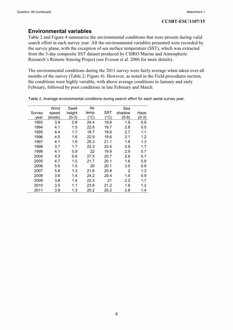
Environmental variables Table 2 and Figure 4 summarize the environmental conditions that were present during valid

search effort in each survey year. All the environmental variables presented were recorded by

the survey plane, with the exception of sea surface temperature (SST), which was extracted

from the 3-day composite SST dataset produced by CSIRO Marine and Atmospheric

Research’s Remote Sensing Project (see Eveson et al. 2006 for more details).

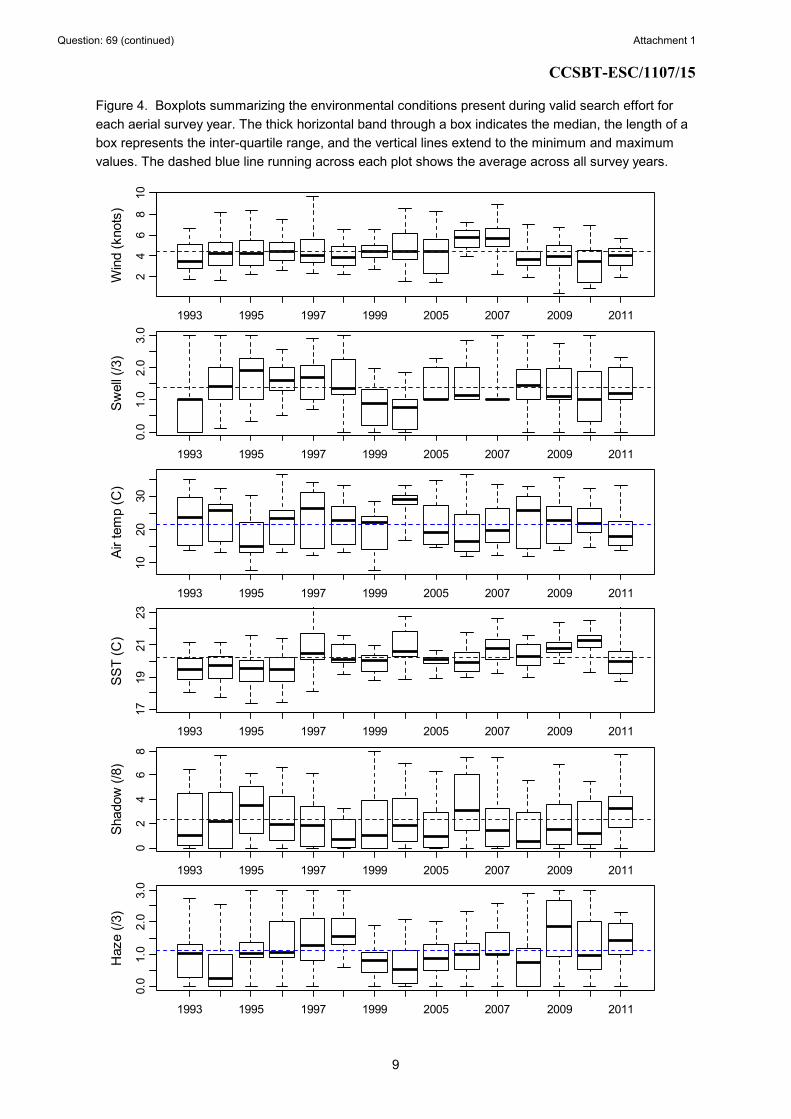
The environmental conditions during the 2011 survey were fairly average when taken over all

months of the survey (Table 2; Figure 4). However, as noted in the Field procedures section,

the conditions were highly variable, with above average conditions in January and early

February, followed by poor conditions in late February and March.

Table 2. Average environmental conditions during search effort for each aerial survey year.

Survey year

Wind speed (knots)

Swell height (0-3)

Air temp

(°C) SST

(°C)

Sea shadow

(0-8) Haze (0-3)

1993 3.9 0.8 24.4 19.6 1.9 0.9

1994 4.1 1.5 22.6 19.7 2.8 0.5

1995 4.4 1.7 18.7 19.6 2.7 1.1

1996 4.5 1.6 22.9 19.6 2.1 1.2

1997 4.1 1.6 25.3 21.1 1.6 1.3

1998 3.7 1.7 22.3 20.4 0.9 1.7

1999 4.1 0.9 22 19.9 2.9 0.7

2000 4.3 0.6 27.5 20.7 2.6 0.7

2005 4.7 1.5 21.7 20.1 1.6 0.8

2006 5.6 1.5 20 20.1 3.5 0.9

2007 5.8 1.3 21.6 20.8 2 1.3

2008 3.8 1.4 24.2 20.4 1.4 0.9

2009 3.8 1.4 22.3 21 2.2 1.7

2010 3.5 1.1 23.6 21.2 1.8 1.2

2011 3.9 1.3 20.2 20.2 2.8 1.4


CCSBT-ESC/1107/15

9

Figure 4. Boxplots summarizing the environmental conditions present during valid search effort for

each aerial survey year. The thick horizontal band through a box indicates the median, the length of a

box represents the inter-quartile range, and the vertical lines extend to the minimum and maximum

values. The dashed blue line running across each plot shows the average across all survey years.

1993 1995 1997 1999 2005 2007 2009 2011

24

68

10

Wind (knots)

1993 1995 1997 1999 2005 2007 2009 2011

0.0

1.0

2.0

3.0

Swell (/3)

1993 1995 1997 1999 2005 2007 2009 2011

10

20

30

Air temp (C)

1993 1995 1997 1999 2005 2007 2009 2011

17

19

21

23

SST (C)

1993 1995 1997 1999 2005 2007 2009 2011

02

46

8

Shadow (/8)

1993 1995 1997 1999 2005 2007 2009 2011

0.0

1.0

2.0

3.0

Haze (/3)


CCSBT-ESC/1107/15

10

Methods of analysis

The methods of analysis this year follow the methods described last year for including data

from one-observer flights, with a few small changes. Details of the methods can be found in

Appendix A, but here we give a brief description highlighting where the analysis has been

changed.

We fit generalized linear models to two different components of observed biomass—biomass

per sighting (BpS) and sightings per nautical mile of transect line (SpM). We included the

same environmental and observer variables in the models as in the past several years. The

only change is that in the SpM model we include “observer effect” as an offset (i.e., as

known) rather than as a linear covariate. The reason for this is discussed in Appendix A.

Because of this, we need to account for uncertainty in the observer effect estimates through

other methods. Such methods have been developed but we were not successful in

implementing them in time for this report. Thus, the standard errors, CVs and confidence

intervals for the relative abundance indices reported in Table 3 do not include uncertainty in

the observer effects for the SpM model (meaning they are slightly too small).

Specifically, the models can be expressed as:

BpS model: logE(Biomass) ~ Year*Month*Area + SST + WindSpeed

SpM model: logE(N_sightings) ~ offset(log(Distance) + log(ObsEffect)) +

Year*Month*Area + SST + WindSpeed + Swell + Haze + MoonPhase

Year, Month, Area and MoonPhase were fit as factors; all other explanatory variables were fit

as linear covariates. Note that the term Year*Month*Area encompasses all 1-way, 2-way and

3-way interactions between Year, Month and Area (i.e., it is equivalent to writing Year +

Month + Area + Year:Month + Year:Area + Month:Area + Year:Month:Area).

In both models, the 2-way and 3-way interaction terms between Year, Month and Area were

fit as random effects, whereas the 1-way effects were fit as fixed effects. Many of the 2-way

and 3-way strata have very few (sometimes no) observations, which causes instabilities in the

model fits when treated as fixed effects. One main advantage of using random effects is that

when little or no data exist for a given level of a term (say for a particular area and month

combination of the Area:Month term), we still have information about it because we are

assuming it comes from a normal distribution with a certain mean and variance (estimated

within the model).

In order to account for including data from one-observer flights, the only change to the BpS

model is that there is only one biomass estimate per school, so it is not necessary to take an

average over the estimates made by two observers (refer to “Biomass per sighting (BpS)

model” section in Appendix A).

With regard to the SpM model, we know from the calibration experiments conducted in 2008

and 2009 that a plane with only one observer makes fewer sightings than a plane with two

observers. Based on an analysis of the calibration experiment data conducted in 2009, we

estimated that, on average, a plane with one observer will make about half as many sightings

as a plane with two observers (Eveson et al. 2009). We referred to this factor as the


CCSBT-ESC/1107/15

11

“calibration factor”. The presence of many large schools of SBT this year (Figure 2) led us to

reconsider our calibration experiment results, since a plane with one spotter seems less likely

to miss very large schools (in fact, it was the spotters involved in this year’s survey who

raised this issue). Re-analysing the data from the calibration experiments leaving out

sightings of small schools confirmed that the calibration factor (i.e., the proportion of

sightings made by one observer compared to two observers) did indeed increase when small

sightings were excluded (Figure 5). We can see that the estimates increase rapidly when really

small sightings are left out of the analysis (<2 t), then start to level off. We fit a power curve

through the data, and used the fitted value corresponding to a sightings cut-off of 2 t, namely

0.7, as our revised calibration factor estimate (i.e., a plane with only one observer makes

approximately 70% as many sightings as a plane with two observers).

Figure 5. Estimated proportion of sightings made by one observer compared to two observers (i.e.,

calibration factor) when small sightings (less than x tonnes for various values of x) are omitted from

the analysis. The red line is a power curve fit through the point estimates.

Note that using 0.7 instead of 0.5 as the calibration factor is a more robust approach because

even if one observer only sees 50% as many really small schools as two observers, but we

assume he sees 70%, this equates to very little difference in overall “missed” biomass.

However, on the contrary, if we assume one observer sees only 50% as many big schools as

0.4

0.5

0.6

0.7

0.8

0.9

Omit sightings < x tonnes

Calibration factor

0 2 5 10 15 20 25


CCSBT-ESC/1107/15

12

two observers, when in fact he sees 70% as many, we will be overestimating the amount of

missed biomass by a lot.

Once the calibration factor has been estimated, it is used to calculate a relative sighting ability

(i.e., an “observer effect”) estimate for solo observers. Recall that the “observer effect”

estimates for the SpM model are calculated based on a pair-wise observer analysis to estimate

the relative sighting abilities of all observer pairs that have been involved in past surveys (see

Appendix A). In order to estimate a relative sighting ability for a solo observer, we took the

average of the relative sighting ability estimates from when he flew as part of a pair, and

multiplied it by the estimated calibration factor. For example, one of the observers who flew

as a solo observer in the 2010 and 2011 surveys has flown as part of two different observer

pairs in past surveys, with relative sighting ability estimates of 0.90 and 0.92. If we take the

average of these two relative sighting ability estimates and multiply it by the calibration factor

of 0.7, this gives a relative sighting ability estimate for this observer when flying solo of 0.64

Thus, we now have “observer effect” estimates for all observer combinations, so we can

proceed with fitting the SpM model in the usual way.

Once the models were fitted, the results were used to predict what the number of sightings per

mile and the average biomass per sighting in each of the 45 area/month strata in each survey

year would have been under standardized environmental/observer conditions. Using these

predicted values, we calculated an abundance estimate for each stratum as ‘standardized

SpM’ multiplied by ‘standardized average BpS’. We then took the weighted sum of the

stratum-specific abundance estimates over all area/month strata within a year, where each

estimate was weighted by the geographical size of the stratum in nm2, to get an overall

abundance estimate for that year. Lastly, the annual estimates were divided by their mean to

get a time series of relative abundance indices.

We emphasise that it is important to have not only an estimate of the relative abundance

index in each year, but also of the uncertainty in the estimates. We used the same process as

last year to calculate CVs for the indices, except we now include uncertainty in the calibration

factor estimate, details of which can be found in Appendix B. Recall from above that there is

still uncertainty in the observer effect estimates (now being input to the SpM model as an

offset) that are not currently being accounted for.

We calculated confidence intervals for the indices based on the assumption that the logarithm

of the indices follows a normal distribution, with standard errors approximated by the CVs of

the untransformed indices.

Results

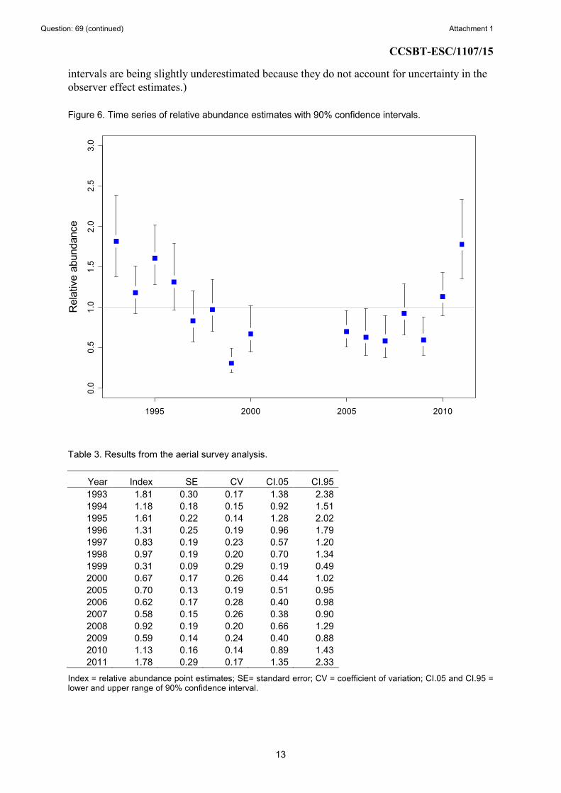
(Model results and diagnostics for the BpS and SpM models are provided in Appendix C.)

Figure 6 shows the estimated time series of relative abundance indices with 90% confidence

intervals. The point estimates and CVs corresponding to Figure 6 are given in Table 3.

The 2011 point shows a substantial increase from 2010 and is similar to the 1993 estimate,

which was the highest estimate of all survey years. The confidence interval on the 2011

estimate is quite wide, but taking this into account, it is still significantly higher than other

estimates in the 2000s. (We should recall from the Methods section that all of the confidence


CCSBT-ESC/1107/15

13

intervals are being slightly underestimated because they do not account for uncertainty in the

observer effect estimates.)

Figure 6. Time series of relative abundance estimates with 90% confidence intervals.

1995 2000 2005 2010

0.0

0.5

1.0

1.5

2.0

2.5

3.0

Relative abundance

Table 3. Results from the aerial survey analysis.

Year Index SE CV CI.05 CI.95

1993 1.81 0.30 0.17 1.38 2.38

1994 1.18 0.18 0.15 0.92 1.51

1995 1.61 0.22 0.14 1.28 2.02

1996 1.31 0.25 0.19 0.96 1.79

1997 0.83 0.19 0.23 0.57 1.20

1998 0.97 0.19 0.20 0.70 1.34

1999 0.31 0.09 0.29 0.19 0.49

2000 0.67 0.17 0.26 0.44 1.02

2005 0.70 0.13 0.19 0.51 0.95

2006 0.62 0.17 0.28 0.40 0.98

2007 0.58 0.15 0.26 0.38 0.90

2008 0.92 0.19 0.20 0.66 1.29

2009 0.59 0.14 0.24 0.40 0.88

2010 1.13 0.16 0.14 0.89 1.43

2011 1.78 0.29 0.17 1.35 2.33

Index = relative abundance point estimates; SE= standard error; CV = coefficient of variation; CI.05 and CI.95 = lower and upper range of 90% confidence interval.


CCSBT-ESC/1107/15

14

Summary

The estimate of relative juvenile abundance from the 2011 scientific aerial survey shows a

substantial increase from 2010 and is similar to the 1993 estimate, which was the highest

estimate of all survey years. The confidence interval on the 2011 estimate is quite wide, but

taking this into account, it is still significantly higher than other estimates in the 2000s.

The 2011 survey was the first in which all flights had only one spotter (i.e., no flights had a

spotter-pilot). Calibration experiments conducted in 2008 and 2009 showed that a plane with

only one spotter makes fewer sightings than a plane with two spotters. We call the proportion

of sightings made by one spotter compared to two spotters the “calibration factor”. A method

of estimating the calibration factor and accounting for it in our analysis of the survey data was

developed in Eveson et al. (2009, 2010). A very high proportion of large schools this year led

us to reconsider the calibration factor reported in Eveson et al. (2010), because a plane with

one spotter is less likely to miss very large schools. Re-analysing the data from the calibration

experiments leaving out very small sightings (<2 tonnes) led to a revised calibration factor

estimate of 0.7 instead of 0.5. Methods to incorporate uncertainty in the calibration factor

estimate were also developed and applied this year, so the CVs for the relative abundance

estimates include this additional uncertainty.

This year’s data included a high proportion of schools comprised of small (<8 kg, estimated

to be 1-year-old) fish, which was unusual compared to past survey years. In the CCSBT OM

and MP, the aerial survey index is assumed to provide a relative time series of age 2-4

abundance in the Great Australian Bight. Thus, for consistency with the OM and MP as well

as general consistency in interpretation of the index across years, schools of 1-year-old fish

(in all years) were omitted from the analysis.

The only other change to the analysis compared to last year is that the observer effect

estimates for the sightings (SpM) model are now being included as an offset (i.e., as known)

rather than as a linear covariate. The reason for this is discussed in Appendix A. As a result,

we need to account for uncertainty in the observer effect estimates through other methods.

Such methods have been developed but we were not successful in implementing them in time

for this report. Thus, the CVs for the relative abundance indices reported here do not yet

include uncertainty in the observer effects for the SpM model (i.e., they are slightly too

small).

References

Anonymous. 2008. Report of the Thirteenth Meeting of the Scientific Committee,

Commission for the Conservation of Southern Bluefin Tuna, 5-12 September 2008,

Rotorua, New Zealand.

Basson, M., Bravington, M., Eveson, P. and Farley, J. 2005. Southern bluefin tuna

recruitment monitoring program 2004-05: Preliminary results of Aerial Survey and

Commercial Spotting data. Final Report to DAFF, June 2005.

Bravington, M. 2003. Further considerations on the analysis and design of aerial surveys for

juvenile SBT in the Great Australian Bight. RMWS/03/03.


CCSBT-ESC/1107/15

15

Cowling, A. 2000. Data analysis of the aerial surveys (1993-2000) for juvenile southern

bluefin tuna in the Great Australian Bight. RMWS/00/03.

Cowling A., Hobday, A., and Gunn, J. 2002. Development of a fishery independent index of

abundance for juvenile southern bluefin tuna and improvement of the index through

integration of environmental, archival tag and aerial survey data. FRDC Final Report

96/111 and 99/105.

Eveson, P. 2011. Updated growth estimates for the 1990s and 2000s, and new age-length cut-

points for the operating model and management procedures. CCSBT-ESC/1107/09.

Eveson, P., Bravington, M. and Farley, J. 2006. The aerial survey index of abundance:

updated analysis methods and results. CCSBT-ESC/0609/16.

Eveson, P., Farley, J., and Bravington, M. 2009. The aerial survey index of abundance:

updated analysis methods and results. CCSBT-ESC/0909/12.

Eveson, P., Farley, J., and Bravington, M. 2010. The aerial survey index of abundance:

updated analysis methods and results for the 2009/10 fishing season.

CCSBT-ESC/1009/14.

Farley, J., Eveson, P. and Clear, N. 2011. An update on Australian otolith collection

activities, direct ageing and length at age in the Australian surface fishery.

CCSBT-ESC/1107/17.

Robins, J.P. 1963. Synopsis of biological data on bluefin tuna, Thunnus thynnus maccoyii

(Castlenau) 1872. FAO Fisheries Report 6: 562:587.

Acknowledgements

There are many people we would like to recognise for their help and support during this

project. We would especially like to thank this year’s observers (spotters), pilots and data

recorders; Andrew Jacob, Darren Tressider, Derek Hayman, John Veerhius, Thor Carter and

Jarred Wait. This study was funded by AFMA, DAFF, the Australian SBT Industry, and

CSIRO’s Wealth from Oceans Flagship.


CCSBT-ESC/1107/15

16

Appendix A – Methods of analysis

Separate models were constructed to describe two different components of observed biomass:

i) biomass per patch sighting (BpS), and ii) sightings per nautical mile of transect line (SpM).

Each component was fitted using a generalized linear model (GLM), as described below.

Since environmental conditions affect what proportion of tuna are available at the surface to

be seen, as well as how visible those tuna are, and since different observers can vary both in

their estimation of school size and in their ability to see tuna patches, the models include

‘corrections’ for environmental and observer effects in order to produce standardized indices

that can be meaningfully compared across years.

For the purposes of analysis, we defined 45 area/month strata: 15 areas (5 longitude blocks

and 3 latitude blocks, as shown in Figure A1) and 3 months (Jan, Feb, Mar). The latitudinal

divisions were chosen to correspond roughly to depth strata (inshore, mid-shore and shelf-

break).

Figure A1. Plot showing the 15 areas (5 longitudinal bands and 3 latitudinal bands) into which the aerial survey is divided for analysis purposes. The green vertical lines show the official transect lines for the surveys conducted in 1999 and onwards; the lines for previous survey years are similar but are slightly more variable in their longitudinal positions and also do not extend quite as far south (which is why the areas defined for analysis, which are common to all survey years, do not extend further south).

128 130 132 134 136

-36

-35

-34

-33

-32

-31

Longitude

Latitude

PortLincoln

Ceduna


CCSBT-ESC/1107/15

17

Biomass per sighting (BpS) model

For the BpS model, we first estimated relative differences between observers in their

estimates of patch size (using the same methods as described in Bravington 2003). As in

Bravington (2003), we found good consistency between observers. In particular, patch size

estimates made by different observers tended to be within about 5% of each other, except for

one observer, say X, who tended to underestimate patch sizes relative to other observers by

about 20%. The patch size estimates were corrected using the estimated observer differences

(e.g. patch size estimates made by observer X were scaled up by 20%). Because the observer

differences were estimated with high precision, we treated the corrected patch size estimates

as exact in our subsequent analyses. The final biomass estimate for each patch was calculated

as the average of the two corrected estimates (recall that the size of a patch is estimated by

both observers in the plane). The final patch size estimates were then aggregated within

sightings to give an estimate of the total biomass of each sighting. It is the total biomass per

sighting data that are used in the BpS model.

The BpS model was fitted using a GLMM (generalized linear mixed model) with a log link

and a Gamma error structure. We chose to fit a rather rich model with 3-way interaction

terms between year, month and area. This is true not only for the BpS model but also for the

SpM model described below. In essence, the 3-way interaction model simply corrects the

observation (the total biomass of a sighting in the case of the BpS model; the number of

sightings in the case of the SpM model) for environmental effects, which are estimated from

within-stratum comparisons (i.e. within each combination of year, month and area).

The 2-way and 3-way interaction terms between Year, Month and Area were fit as random

effects, whereas the 1-way effects were fit as fixed effects. Many of the 2-way and 3-way

strata have very few (sometimes no) observations, which causes instabilities in the model fits

when treated as fixed effects. One main advantage of using random effects is that when little

or no data exist for a given level of a term (say for a particular area and month combination of

the Area:Month term), we still have information about it because we are assuming it comes

from a normal distribution with a certain mean and variance (estimated within the model).

Having decided on the overall structure, we then decided what environmental variables to

include in the model. Based on exploratory plots and model fits, we determined the two

environmental covariates that had a significant effect on the biomass per sighting were wind

speed and, especially, SST.1 Thus, the final model fitted was

logE(Biomass) ~ Year*Month*Area + SST + WindSpeed

where Year, Month and Area are factors, and SST and WindSpeed are linear covariates (note

that E is standard statistical notation for expected value).

Sightings per mile (SpM) model

For the SpM model, we first updated the pairwise observer analysis described in Bravington

(2003), based on within-flight comparisons of sighting rates between the various observers. 1 Note that the selection of environmental covariates for the BpS and SpM models was undertaken as part of the

2006 analysis. We re-investigated last year (see Eveson et al. 2010) and found some suggestion that wind speed

was not necessary in the BpS model and that sea shadow should be included in the SpM model, but we have

chosen to keep the covariates the same for now for consistency purposes, and because it made very little

difference to the relative abundance estimates.


CCSBT-ESC/1107/15

18

This analysis gives estimates of the relative sighting efficiencies for the 18 different observer

pairs that have flown at some point in the surveys. The observer pairs ranged in their

estimated sighting efficiencies from 72% to 97% compared to the pair with the best rate.

This year, we include the (logged) estimates of relative observer pair efficiencies as an offset

when fitting the SpM model (i.e., as a predictor variable with a known, rather than estimated,

coefficient). In past, we have included the logged estimates as a covariate in the SpM model

rather than as an offset, with the coefficient (i.e., “slope”) to be estimated, with the notion that

if the relative efficiencies from the pairwise analysis are correct, the slope estimate should be

close to one. By doing so, we were attempting to capture some of the uncertainty in the

estimates. As discussed in last year’s report (Eveson et al. 2010), the coefficient of the log

observer effect term was actually coming out close to negative one, and although it was

coming out as insignificant, this was still a worry because it suggests that the sightings rate

actually declines as our estimates of relative sighting ability increases. Complex interactions

between the space-time strata and the observer effects seemed to be the cause of this. As

such, we have chosen to include the log relative efficiencies as an offset, and account for their

uncertainty through other methods. Such methods have been developed but we were not

successful in implementing them in time for this report. Thus, the standard errors and CVs for

the relative abundance indices reported in Table 3 do not include uncertainty in the observer

effects for the SpM model (which means they are slightly too small). We aim to get the

methods of including observer uncertainty implemented correctly in the coming year.

The data used for the SpM model were accumulated by flight and area, so that the data set

used in the analysis contains a row for every flight/area combination in which search effort

was made (even if no sightings were made). Within each flight/area combination, the number

of sightings and the distance flown were summed, whereas the environmental conditions

were averaged. The SpM model was fitted using a GLMM with the number of sightings as

the response variable, as opposed to the sightings rate. The model could then be fitted

assuming an overdispersed Poisson error structure2 with a log link and including the distance

flown as an offset term to the model (i.e. as a linear predictor with a known coefficient of

one).

As we did for the BpS model, we included terms for year, month and area, as well as all

possible interactions between them, in the SpM model, and we fitted the 2-way and 3-way

interaction terms as random effects (see BpS model section). We determined what

environmental variables to include in the model based on exploratory plots and model fits

(see footnote 1). The final model fitted was:

logE(N_sightings) ~ offset(log(Distance) + log(ObsEffect)) + Year*Month*Area

+ SST + WindSpeed + Swell + Haze + MoonPhase

where Year, Month and Area are factors, MoonPhase is a factor (taking on one of four levels

from new moon to full moon), and all other terms are linear covariates. Note, as discussed

above, that the log observer effect estimates are now being included as an offset rather than a

linear covariate.

2 Note that the standard Poisson distribution has a very strict variance structure in which the variance is equal to

the mean, and it would almost certainly underestimate the amount of variance in the sightings data, hence the use

of an overdispersed Poisson distribution to describe the error structure.


CCSBT-ESC/1107/15

19

Combined analysis

The BpS and SpM model results were used to predict what the number of sightings per mile

and the average biomass per sighting in each of the 45 area/month strata in each survey year

would have been under standardized environmental/observer conditions3. Using these

predicted values, we calculated an abundance estimate for each stratum as ‘standardized

SpM’ multiplied by ‘standardized average BpS’. We then took the weighted sum of the

stratum-specific abundance estimates over all area/month strata within a year, where each

estimate was weighted by the geographical size of the stratum in nm2, to get an overall

abundance estimate for that year. Lastly, the annual estimates were divided by their mean to

get a time series of relative abundance indices.

3 In our predictions, we used average conditions calculated from all the data.


CCSBT-ESC/1107/15

20

Appendix B – CV calculations

This appendix provides details of how CVs for the aerial survey abundance indices were

calculated.

Let îjkB be the predicted value of BpS in year i, month j and area k under standardized

environmental/observer conditions (see footnote 3), and ( )ˆîjkBσ be its estimated standard

error. Similarly, let îjkS be the predicted value of SpM in year i, month j and area k under the

same environmental/observer conditions, and ( )ˆîjkSσ be its estimated standard error. Then,

ˆ ˆ îjk ijk ijkA S B=

is the stratum-specific abundance estimate for year i, month j and area k.

Since îjkB and îjkS are independent, the variance of îjkA is given by

( ) ( )( ) ( ) ( ) ( ) ( ) ( )( ) ( ) ( ) ( )

22

2 2 2 2 2 2

ˆ ˆ ˆ

ˆ ˆ ˆˆ ˆ ˆ

ˆ ˆ ˆˆ ˆ ˆˆ ˆ ˆ ˆ

ijk ijk ijk

ijk ijk ijk ijk ijk ijk

ijk ijk ijk ijk ijk ijk

V A V S B

V S E B V B E S V S V B

S B B S S Bσ σ σ σ

=

= + +

≈ + +

The annual abundance estimate for year i is given by the weighted sum of all stratum-specific

abundance estimates within the year, namely

ˆ î k ijk

j k

A w A=∑∑

where kw is the proportional size of area k relative to the entire survey area ( 1k

k

w =∑ ).

If the îjkA ’s are independent, then the variance of îA is given by

( ) ( )2ˆ î k ijk

j k

V A w V A=∑∑

Unfortunately, the îjkA ’s are NOT independent because the estimates of BpS (and likewise,

the estimates of SpM) are not independent between different strata. This is because all strata

estimates depend on the estimated coefficients of the environmental/observer conditions, so

any error in these estimated coefficients will affect all strata. Thus, we refit the BpS and SpM

models with the coefficients of the environmental/observer covariates (denote the vector of

coefficients by θ 4) fixed at their estimated values (θ̂ ). The predictions of BpS and SpM

4 θ contains the environmental/observer coefficients from both the BpS and SpM models; i.e.

BpS SpM( , )θ θ θ=


CCSBT-ESC/1107/15

21

made using the ‘fixed environment’ models should now be independent between strata, so the

stratum-specific abundance estimates calculated using these predictions – which we will

denote by ( )ˆ îjkA θ – should also be independent between strata. Thus, we can calculate the

variance of îA conditional on the estimated values of the environmental/observer coefficients

as

( ) ( )( )2ˆ ˆ ˆ ˆ|i k ijk

j k

V A w V Aθ θ=∑∑

where ( )( )ˆ îjkV A θ is calculated using the formula given above for ( )ˆ

ijkV A but using the BpS

and SpM predictions and standard errors obtained from the ‘fixed environment’ models.

To calculate the unconditional variance of îA , we make use of the following equation:

( ) ( )( ) ( )( )( ) ( )

ˆ ˆ ˆ| |

ˆ ˆ ˆ|

i i i

i i

V A E V A V E A

V A V A

θ θ

θ

θ θ

θ

= +

≈ +

where the first term is the conditional variance just discussed and the second term is the

additional variance due to uncertainty in the environmental coefficients. The second term can

be estimated as follows

( )ˆ ˆ

ˆ i i

i

A AV Aθ θθ θ

′ ∂ ∂≈ ∂ ∂

V

where îA

θ

∂ ∂

is the vector of partial derivatives of îA with respect to θ (which we calculated

using numerical differentiation), and θV is the variance-covariance matrix of the

environmental coefficients5.

Now, to account for the additional variance due to uncertainty in the calibration factor, we use

a similar approach as above to account for additional variance due to uncertainty in the

environmental coefficients. Namely, from the GLM used to estimate the calibration factor,

which we will call α , we get an estimate of its variance, which we will call Vα . Then, the

variance in the abundance estimates due to uncertainty in α can be estimated by

( )ˆ î i

i

A AV A Vα αα α

′ ∂ ∂= ∂ ∂

)

5 Recall that θ contains the environmental/observer coefficients from both the BpS and SpM models, so

BpS

SpM

θ

θ

θ

=

V 0

V0 V

. The variance-covariance matrices for the individual models are returned from the model-

fitting software.


CCSBT-ESC/1107/15

22

where îA

α

∂ ∂

is the derivative of îA with respect to α (in essence, it is the amount that the

abundance estimate îA changes when the calibration factor is tweaked slightly). Thus, we

revise our estimate of ( )îV A by adding on to it ( )iV Aα

).

So we have variance estimates for the abundance estimates, but we also want to calculate the

variance for the mean-standardized estimates (referred to as the relative abundance indices),

calculated as:

1

ˆˆ

1 ˆ

ii n

i

i

AI

An =

=

∑

Using the delta method, we can approximate the variance of îI by

( ) ( )2

ˆˆˆ

î

i i

i

IV I V A

A

∂≈ ∂

Then, the standard error of îI is given by

( ) ( )ˆ î iI V Iσ =

and the coefficient of variation (CV) of îI is given by

( ) ( )ˆˆCV

ˆ

i

i

i

II

I

σ= .


CCSBT-ESC/1107/15

23

Appendix C: Results and diagnostics

Biomass per sighting (BpS) model

Extract from the output produced by the software used to fit the model (the gam function in the R statistical package mgcv): Family: Gamma Link function: log Formula: Biomass ~ factor(Year) + factor(Month) + factor(Area) + SST + WindSpeed + Y.M + Y.A + M.A + Y.M.A - 1 Parametric Terms:

Covariate Estimate SE t-value p-value

SST 0.128 0.041 3.092 0.002

WindSpeed -0.043 0.026 -1.699 0.090

R-sq.(adj) = 0.0828 Deviance explained = 38.6% GCV score = 2.0143 Scale est. = 1.7649 n = 1637

The results suggest that the size of a sighting tends to increase as SST increases and decrease

as wind speed increases, but that relationship with SST has much greater statistical

significance. These results are roughly supported by plots of observed biomass per sighting

(on a log scale) versus the environmental covariates. Nevertheless, we prefer to include wind

speed in the model for consistency with previous years, and because the relative abundance

estimates were very similar when wind speed was omitted.

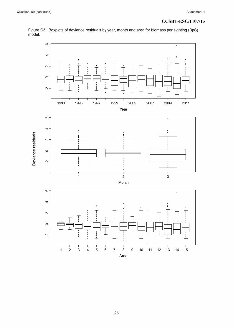
Figure C2 shows some standard diagnostic plots for generalized linear models, and Figure C3

shows the residuals plotted against a number of factors. These plots do not suggest major

problems with the model fit. Ideally there should be no trend in the plots of the square root of

the absolute residuals against the fitted values (i.e., lower half of Fig. C2, with left-hand side

being on the link scale and the right-hand side being on the response scale); although there is

a small kink revealed by a smooth through the data (red line), there is not a consistent

increasing or decreasing trend.


CCSBT-ESC/1107/15

24

Figure C1. Plots of observed biomass per sighting, on a log scale, versus the covariates included in the model; shown is the mean +/- 2 standard deviations.

18 19 20 21 22 23 24 25

2.5

3.0

3.5

4.0

4.5

SST

log(BpS)

0 2 4 6 8

1.0

1.5

2.0

2.5

3.0

3.5

4.0

INT_WindSpeedlog(BpS)


CCSBT-ESC/1107/15

25

Figure C2. Standard diagnostic plots for biomass per sighting (BpS) model.

-4 -2 0 2 4

-20

24

6

theoretical quantiles

deviance residuals

Deviance residualsFrequency

-4 -2 0 2 4 6

0100

200

300

400

500

0 1 2 3 4 5 6

0.0

0.5

1.0

1.5

2.0

linear predictor

sqrt(abs(deviance resids))

0 100 200 300 400

01

23

4

fitted

sqrt(abs(pearson resids))


CCSBT-ESC/1107/15

26

Figure C3. Boxplots of deviance residuals by year, month and area for biomass per sighting (BpS) model.

1993 1995 1997 1999 2005 2007 2009 2011

-20

24

6

Year

1 2 3

-20

24

6

Month

1 2 3 4 5 6 7 8 9 10 11 12 13 14 15

-20

24

6

Area

Deviance residuals


CCSBT-ESC/1107/15

27

Sightings per mile (SpM) model

Extract from the output produced by the software used to fit the model (the gam function in the R statistical package mgcv): Family: quasipoisson Link function: log Formula: N_sightings ~ offset(log(as.numeric(Distance))) + factor(Year) + factor(Month) + factor(Area) + Y.M + Y.A + M.A + Y.M.A + log(ObserverEffect) + AvgWindSpeed + AvgSST + AvgSwell + AvgHaze + factor(MoonPhase) - 1 Parametric Terms:

Covariate Estimate SE t-value p-value

AvgWindSpeed -0.262 0.023 -11.209 0.000

AvgSST 0.211 0.036 5.913 0.000

AvgSwell -0.189 0.055 -3.452 0.001

AvgHaze -0.122 0.049 -2.471 0.014

factor(MoonPhase)2 -0.127 0.102 -1.247 0.213

factor(MoonPhase)3 -0.008 0.126 -0.064 0.949

factor(MoonPhase)4 0.186 0.086 2.148 0.032 R-sq.(adj) = 0.475 Deviance explained = 65.7% GCV score = 1.5291 Scale est. = 1.2395 n = 1620

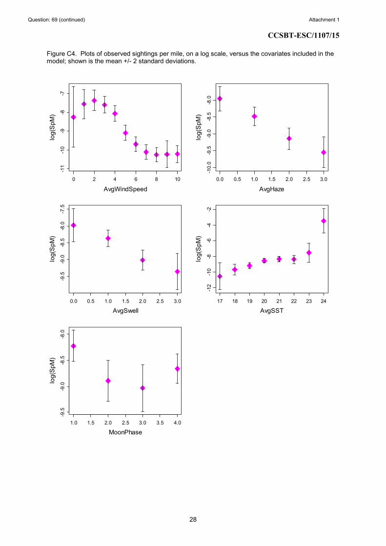
The results suggest that there is a tendency for the rate of sightings to increase as SST

increases, and to decline as wind speed, haze and swell increase (all highly significant). The

relationship with moon phase is more complex, with the sightings rate being greater when the

moon phase is 1 (fraction of moon illuminated is 0-25%) or 4 (fraction of moon illumination

is 75-100%), but this relationship is not as significant.

Figure C5 shows some standard diagnostic plots for generalized linear models, and Figure C6

shows the residuals plotted against a number of factors. The Q-Q plot has a funny kink, but

otherwise there are no indications of serious problems with the model fit. The plots of the

square root of the absolute residuals against the fitted values (i.e., lower half of Fig. C5, with

left-hand side being on the link scale and the right-hand side being on the response scale)

look a bit odd, but this is expected because we are modelling count data. A smooth line

through these data is reasonably flat, as desired, except for where it follows the residuals for

the zero response values (i.e., where the observed number of sightings was zero).


CCSBT-ESC/1107/15

28

Figure C4. Plots of observed sightings per mile, on a log scale, versus the covariates included in the model; shown is the mean +/- 2 standard deviations.

0 2 4 6 8 10

-11

-10

-9-8

-7

AvgWindSpeed

log(SpM)

0.0 0.5 1.0 1.5 2.0 2.5 3.0

-10.0

-9.5

-9.0

-8.5

-8.0

AvgHaze

log(SpM)

0.0 0.5 1.0 1.5 2.0 2.5 3.0

-9.5

-9.0

-8.5

-8.0

-7.5

AvgSwell

log(SpM)

17 18 19 20 21 22 23 24

-12

-10

-8-6

-4-2

AvgSST

log(SpM)

1.0 1.5 2.0 2.5 3.0 3.5 4.0

-9.5

-9.0

-8.5

-8.0

MoonPhase

log(SpM)


CCSBT-ESC/1107/15

29

Figure C5. Standard diagnostics plots for sightings per mile (SpM) model.

-3 -2 -1 0 1 2 3

-4-2

02

4Normal Q-Q Plot

Theoretical Quantiles

deviance residuals

Deviance residualsFrequency

-4 -2 0 2 4 6

0200

400

600

800

1000

-3 -2 -1 0 1 2 3

0.0

0.5

1.0

1.5

2.0

linear predictor

sqrt(abs(deviance resids))

0 5 10 15

0.0

0.5

1.0

1.5

2.0

2.5

3.0

fitted

sqrt(abs(pearson resids))


CCSBT-ESC/1107/15

30

Figure C6. Boxplots of deviance residuals by year, month and area for sightings per mile (SpM) model.

1993 1995 1997 1999 2005 2007 2009 2011

-4-2

02

4

Year

1 2 3

-4-2

02

4

Month

1 2 3 4 5 6 7 8 9 10 11 12 13 14 15

-4-2

02

4

Area

Deviance residuals




Question: 152 Division/Agency: ABARES − Australian Bureau of Agricultural and Resource Economics and Sciences Topic: Forecast for forest products Proof Hansard page: Written Senator COLBECK asked:

3. What length of time would forecasts cover? Answer: 1. Yes. At the ABARES−Forest and Wood Products Australia (FWPA) Project Steering

Committee meeting on 5 July 2011, the need for developing forecasts of consumption and trade of main forest products was discussed, as part of the forest data project.

2. It was agreed that ABARES would use econometric modelling techniques based on key

economic indicators to develop consumption and trade forecasting models for sawnwood, wood-based panels, woodchips and paper products. It was agreed that ABARES would seek the Steering Committee’s advice on the methodology. A program of work is being developed for the next 12 months to prepare forecasting models in each of these areas.

3. The forecasts would cover 3 years.

1. The Department advised that there would be consideration of developing forecasts for forest products at a meeting in July 2011. Has this meeting taken place and was the need for developing forecasts for forest products discussed?

2. What was the outcome?



Question: 153 Division/Agency: ABARES – Australian Bureau of Agricultural and Resource Economics and Sciences Topic: Plantations Proof Hansard page: Written Senator COLBECK asked: 1. Given the reduction in Australia’s plantation estate (ABARES media release 31 August

2011) and 2010 seeing the smallest area of new plantations established since the 1990s, what projections have ABARES made regarding the ability of Australia to service its domestic requirements for wood and wood products?

2. Has ABARES undertaken any analysis of the impact of the Tasmanian Forests IGA, with regard to the ability of Australia to service its domestic requirements for wood and wood products?

3. What research has ABARES undertaken in relation to the impact of diminishing domestic timber supplies on the global timber market and the sustainability of global timber supplies?

Answer:

1. Since 1997, ABARES has prepared five-yearly projections of total log supply from plantations. The next report will be released in March 2012 with projections to 2054.

2. The Tasmania Forests Intergovernmental Agreement responds to a commercial decision and market drivers for the industry in Tasmania.

3. None.



Question: 154 Division/Agency: ABARES – Australian Bureau of Agricultural and Resource Economics and Sciences Topic: Agricultural commodities Proof Hansard page: Written Senator COLBECK asked: 1. The Agricultural commodities data for the 2011 September quarter shows farmers’ terms

of trade as negative 4.1% for 2011-12 compared to 2010-11. What impact is this having on the overall sustainability of farming in Australia?

2. Has any assessment been undertaken of environmental and social consequences of these sorts of results?

3. The Agricultural commodities data for the 2011 September quarter shows a 4.8% downturn in employment in agriculture, forestry and fishing for 2010-11 compared to 2009-10. What are the key factors contributing to this downturn in employment?

4. What are the employment changes for each sector? 5. What assessment has ABARES undertaken into the impact of the domestic retail market

on terms of trade for Australian farmers? 6. What assessment has ABARES undertaken into the impact of the domestic retail market

on employment in the agricultural sector? 7. The report highlights price falls for vegetables and milk. What was the extent of these

price falls? 8. How have these reductions impacted on the returns to primary producers? 9. The projected increase of 5.9% in export earnings for forestry products relates to what

type(s) of timber products? 10. The report suggests that significant volatility in the Australian exchange rate is likely to

continue and that it is important for primary producers and exporters to manage the risks associated with fluctuations in the Australian exchange rate. What specific advice does ABARES or other departments have for primary producers and exporters in this regard?

11. What resources / programs does the government have to assist primary producers and exporters?

Answer:

1. The forecast decline of 4.1 per cent in terms of trade for 2011–12 will have minimal impact on the sustainability of farming in Australia. According to agricultural commodities data for the 2011 September quarter, the forecast decline in 2011–12 follows a 14 per cent increase in 2010 –11, when the terms of trade were at a five- year high. The forecast decline for 2011–12—should it eventuate—will see farmers’ terms of trade at a higher level than the period from 2006–07 to 2009 –10. Thus the outlook for Australian producers and the Australian farm sector in 2011–12 remains positive.

2. No.



Question: 154 (continued)

3. The total number of employed persons in the agriculture, forestry and fishing sectors in 2010–11 was released by the Australian Bureau of Statistics (ABS), catalogue number 6291.0.55.003 Labour Force, Australia, Detailed, Quarterly. No specific reasons were provided by the ABS as to why the persons employed in these sectors declined in 2010 –11.

4. ABARES does not have access to the ABS database for a breakdown of the employment changes for each industry included in the agriculture, forestry and fishing sectors.

5. ABARES has not undertaken any analysis of the impact of the domestic retail market on terms of trade for Australian farmers.

6. ABARES has not undertaken any assessment of the impact of the domestic retail market on employment in the agriculture sector.

7. The Australian average farmgate price of milk is forecast to decline by 2.1 per cent in 2011–12 to 42.5 cents a litre. This price forecast is 13.9 per cent higher than the average farmgate price for milk in 2009 –10. The forecast price decline in 2011–12 reflects forecast lower world prices for butter and skim milk powder, and the effects of an assumed appreciation of the Australian dollar. ABARES did not provide forecasts of vegetable prices in 2011–12 in the September 2011 issue of Agricultural Commodities. However, based on information from the Melbourne wholesale market, wholesale prices of a selected basket of vegetables declined in that market by an average of 3 per cent in the September quarter of 2011, compared with the June quarter of 2011, but were 9 per cent higher than in the September quarter of 2010.

8. The impact of forecast lower milk prices on farm incomes is expected to be partially offset by forecast higher milk production in the main dairying regions of Australia in 2011–12. Australian milk production is forecast to increase by around 2.2 per cent to 9300 million litres in 2011–12 reflecting improved seasonal conditions in many of the main dairying regions. Similarly, most vegetable growers are expected to benefit from increased production, due to improved seasonal conditions including a marked recovery in supplies of irrigation water in the Murray-Darling Basin.

9. The projected 5.9 per cent increase in the export earnings for forestry products in 2011–12 relative to 2010 –11 relates to all primary forest products (including sawnwood, wood-based panels, paper and paperboard and woodchips). Note that this projection does not include changes in the export of secondary forest products such as furniture, prefabricated buildings and printed articles.

10. Managing risk is a standard business practice for all businesses and there are numerous

financial services that provide risk-management advice. ABARES, as a government forecasting agency, does not provide any specific business-level advice to primary producers and exporters.




11. The Australian Government recognises that investment in research, development and

extension is vital to helping industry to improve productivity, sustainability and competiveness. In 2008–09 the government provided $715 million to support rural research and development through funding contributions to research and development (R&D) corporations, cooperative research centres, CSIRO, universities, the R&D tax concession and other grants programs. The R&D corporations receive funding for research and development via a co-investment model which the government facilitates through the collection of statutory levies from producers in their relevant industries. A number of the Research and Development Corporations also provide marketing and product promotion services to industry which the government facilitates via the collection of statutory levies from producers in their relevant industries. The government does not match marketing levies. Some of the resources/programs the government has to assist primary producers are FarmReady Reimbursement Grants and FarmReady Industry Grants.



Question: 155 Division/Agency: ABARES – Australian Bureau of Agricultural and Resource Economics and Sciences Topic: Research and development and food security Proof Hansard page: Written Senator COLBECK asked: 1. Dr Terry Sheales (Acting Deputy Executive Director ABARES) claims that public

investment in broadacre R&D and extension can generate average returns as high as 47% a year. Given the magnitude of the impending global food task, and the opportunity for significant returns, why is government R&D funding increasing in actual terms by only about 1% a year?

2. How can Australia position itself to do as Paul Morris (previous Deputy Executive Director of ABARES) suggested and make effective contributions to global food security by providing technical assistance to improve agricultural productivity in developing countries if R&D dollars are reducing in real terms?

3. Can the Minister explain how, against this decline in investment in Australia’s food supply, it is possible to be so confident that the food security of the nation is assured (media release 18 May 2011 “Economic prosperity and trade guarantee Australia’s food security”).

4. Can ABARES explain how they can be so confident that Australia does not have a food security issue when others are suggesting the self sufficiency picture being painted is incorrect?

5. What analysis has been undertaken regarding Australia’s current and projected ability to provide the variety of food currently available to Australian consumers, not just wheat and beef?

6. What analysis has been undertaken of Australia’s current and projected ability to produce enough food to meet the population’s nutritional requirements?

7. What analysis has been undertaken of the ability of Australia’s horticultural sector to meet current and projected domestic dietary requirements?

8. ABARES Agricultural Commodities report for the 2011 September quarter states that Vietnam experienced a 34% year on year increase in food price increases, which have significantly affected the annual inflation rate (23%). What consideration has ABARES given to the potential for civil unrest and the impact that could have on food security?

Answer: 1. The Australian Government has committed to retain the funding arrangements for Rural

Research and Development that were in place under the Howard Government.




This means the current RDC funding model remains, with many industries receiving up to 0.5 per cent of GVP in matching contributions. However, in each case, the level of Government contributions depends on a combination of three ‘caps’: the size of the industry’s GVP, the industry’s R&D expenditure and the amount of levy collected. This model has remained relatively constant since the Primary Industries and Energy Research and Development Act was introduced in 1989.

2. See answer to Question 1.

3. Australia is among the most prosperous economies in the world and produces an

abundance of food which is readily supplemented by imports for which consumers are well able to pay. Australia exports around 55 per cent of its food production (in value terms) to overseas markets.


5. ABARES released a paper titled ‘Global Food Security: facts, issues and implications’ in its Science and Economic Insights publication in 2011, which addresses this question.

6. ABARES released an analysis titled ‘The nutritional value of Australia’s food imports’ in the June 2011 Australian Commodities. In that analysis, the current nutritional value of its imports and domestic production was assessed. The estimates reported in the analysis provide some indication of Australia’s ability to provide for the nutritional requirements of its population.





Question: 156 Division/Agency: ABARES – Australian Bureau of Agricultural and Resource Economics and Sciences Topic: Live exports Proof Hansard page: Written Senator COLBECK asked:

Answer: 1. ABARES farm financial performance analysis and forecasts are based on its annual

Australian Agriculture and Grazing Industries Survey. The preliminary results for the 2010–11 financial year will not be available until December 2011.

2. See response to Question 1. 3. Forecasts of live cattle export numbers and value of exports for 2011–12 are available in

the September quarter issue of Agricultural Commodities and is available at www.abares.gov.au.

4. This question does not relate to a specific area of forecasts. 5. ABARES conducted a survey in late June and early July of beef cattle producers in

northern Australian live cattle export regions and asked the producers in the region about the effects on farm businesses of the suspension of the trade with Indonesia. The survey report is available on the ABARES website at www.abares.gov.au.

6. Some information on the possible impacts on associated industries and communities is

available in the Regulation Impact Statement (RIS) for the livestock exports regulatory framework for animal welfare assurance. The RIS is available on the website of the Office of Best Practice Regulation at www.ris.finance.gov.au /2011/10/21/livestock-exports-regulatory-framework-for-animal-welfare-assurance-%e2%80%93-regulation-impact-statement-and-post-implementation-review-%e2%80%93-department-of-agriculture-fisheries-and-forestry/

1. In June 2011, ABARES were optimistic of an improved financial position for beef producers for the 2010-11 financial year. Did this result eventuate?

2. Were there any flow on impacts to southern producers, who were also set for a better year?

3. Has any reforecasting taken place to account for the ban on live exports? 4. What are the forecasts for the 2011- 12 financial year? 5. Has ABARES undertaken any analysis of the impact of the disruption of live exports to

primary producers and to the terms of trade and employment figures in this sector? 6. What information is available regarding impacts on associated industries and

communities of the live exports ban?



Question: 157 Division/Agency: ABARES – Australian Bureau of Agricultural and Resource Economics and Sciences Topic: Marine parks Proof Hansard page: Written Senator COLBECK asked: 1. Has the socio-economic assessment of the south-west bioregion been completed? 2. If so, what were the key findings? 3. This assessment involves extensive consultation with industry, state agencies and other

stakeholders, please provide details of how this consultation is taking place, who has been approached to be involved, who has been involved and whether what proportion of meetings were confidential or closed meetings.

4. The Media Release 20 July 2011 asked for people to contact the ABARES research team. Which media outlets used this release?

Answer: 1. The social and economic assessment for the south-west bioregion has not been

completed.

2. The report is yet to be completed.

3. The assessment is focused on the potential impacts of the draft marine reserve network on commercial and charter fishing.

The social and economic assessment consultation involves several components: • A South-West Working Group meets every one to two weeks, usually via

teleconference, to progress the assessment and discuss initial results. The Working Group comprises representatives from the Western Australian Fishing Industry Council, the Commonwealth Fisheries Association, Wildcatch South Australia, the Western Australian Government, the South Australian Government, the Department of Sustainability, Environment, Water, Population and Communities and ABARES. These meetings are closed to the public and confidential to the working group members.

• As part of the socio-economic assessment, a survey was sent to 281 potentially affected fishing businesses/operators from which 83 valid responses were received. The list of persons to participate in the survey was drawn up in consultation with the members of the South-West Working Group. Individual responses are confidential.




• ABARES held focus group meetings in Port Lincoln, Streaky Bay, Fremantle, Port Augusta and Esperance. These meetings involved the fishing industry and related services, as well as representatives from the broader community and local government. In total 30 fishing industry and six community representatives attended the focus group meetings. The locations for these meetings were developed through discussions with the fishing industry and the working group.

• Thirty three confidential person-to-person interviews were conducted by ABARES with potentially affected individuals.

• ABARES made presentations to, and participated in, a number of meetings organised by the Western Australian Fishing Industry Council. These meetings have discussed initial results and assisted in identifying and quantifying the range of potential impacts. Parts of these meetings were confined to the fishing industry only, and ABARES did not participate in these.

4. No media outlets contacted ABARES regarding the media release of 20 July 2011.

ABARES did not conduct a review of outlets that used the media release in media articles.



Question: 158 Division/Agency: ABARES – Australian Bureau of Agricultural and Resource Economics and Sciences Topic: Fisheries statistics Proof Hansard page: Written Senator COLBECK asked: Was the 3% fall in value of wild catch, reported in the Australian fisheries statistics 2010, due to lower returns or lower catch volumes? Answer: Lower catch volumes of the high unit value species was the primary reason for a three per cent fall in the value of wild catch production in 2009–10.



Question: 159 Division/Agency: ABARES – Australian Bureau of Agricultural and Resource Economics and Sciences Topic: Vegetable industry survey Proof Hansard page: Written Senator COLBECK asked: The ABARES survey found the average cash income for vegetable farmers rose to $200,000 even though vegetable prices fell. Mr Bowen in an ABC interview said this shows it was the better season not the better prices that drove the increasing farm income.

1. What analysis has ABARES done on regarding returns required to sustain vegetable growers through the years when the season is less than favourable?

2. In this year’s survey growers expressed worries about rising input costs like labour, fuel and fertiliser and marketing, what analysis has ABARES done in this area?

Answer: 1. In general, ABARES surveys of Australian vegetable growing farms have indicated that

although less favourable season conditions result in lower vegetable yields, the prices received by growers tend to be higher because of the reduced supply of vegetables on the market. For example, in 2006–07 and 2007–08, the vegetable industry surveys indicated a higher proportion of growers experienced drought or below average seasonal conditions compared with 2008–09. In these years, crop yields were lower but growers received higher average farmgate prices for vegetables, which helped to largely maintain average farm cash incomes.

2. As part of the survey, ABARES collects data on input costs and reports national average

results in terms of cost of production per tonne for various vegetables. For example, in 2008–09 the estimated cost of producing a tonne of potatoes fell as the quantity of potatoes harvested increased. For potato growers who harvested less than 100 tonnes of potatoes, it cost an average of $837 to produce a tonne of potatoes, compared with around $243 for growers who harvested more than 1000 tonnes of potatoes. Further, ABARES has analysed the importance of the different cost components in producing vegetables. Growers participating in the survey are asked to apportion each of the major cost components to the production of various farm outputs. These costs are aggregated to derive a cost per tonne produced for ten different vegetables. The largest cost components for most vegetables analysed have been hired labour, contracts paid, fertiliser and seed.

Supplementary budget estimates 2011-2012

Documents

Transcript of Supplementary budget estimates 2011-2012