Supplemental text for: Rebnegger C, Vos T, Graf AB, Valli M,...
26
1 Supplemental text for: Rebnegger C, Vos T, Graf AB, Valli M, Pronk JT, Daran-Lapujade P, Mattanovich D. Pichia pastoris exhibits high viability and low maintenance-energy requirement at near-zero specific growth rates Supplemental File Descriptions: Supplemental file 1 MATLAB codes and information on how to use these codes to perform retentostat prediction and non-linear regression analysis (Supplemental Methods). Apparent growth yield and maximum growth rate of the Pichia pastoris CBS 7435 FLO8 and CBS 7435 ∆flo8 strain (Table S1). Viability during retentostat cultivation based on colony- forming unit count (Table S2). Regression analysis on overlapping sets of specific growth rate versus glucose uptake rate relations from 4 data points measured at different consecutive specific growth rates (Fig. S1), morphology of P. pastoris during retentostat cultivation (Fig. S2) and example of non-linear regression analysis of viable biomass for one retentostat (Fig. S3). Supplemental file 2 Excel file Example_retentostat_data.xlsx for non-linear regression analysis. Supplemental file 3 Excel file Microarray_data.xlsx containing microarray data and detailed results of GO term enrichment analysis for cluster A and B.
Transcript of Supplemental text for: Rebnegger C, Vos T, Graf AB, Valli M,...

1
Supplemental text for:
Rebnegger C, Vos T, Graf AB, Valli M, Pronk JT, Daran-Lapujade P, Mattanovich D. Pichia
pastoris exhibits high viability and low maintenance-energy requirement at near-zero
specific growth rates
Supplemental File Descriptions:
Supplemental file 1 MATLAB codes and information on how to use these codes to perform
retentostat prediction and non-linear regression analysis (Supplemental Methods).
Apparent growth yield and maximum growth rate of the Pichia pastoris CBS 7435 FLO8 and
CBS 7435 ∆flo8 strain (Table S1). Viability during retentostat cultivation based on colony-
forming unit count (Table S2). Regression analysis on overlapping sets of specific growth
rate versus glucose uptake rate relations from 4 data points measured at different
consecutive specific growth rates (Fig. S1), morphology of P. pastoris during retentostat
cultivation (Fig. S2) and example of non-linear regression analysis of viable biomass for one
retentostat (Fig. S3).
Supplemental file 2 Excel file Example_retentostat_data.xlsx for non-linear regression
analysis.
Supplemental file 3 Excel file Microarray_data.xlsx containing microarray data and detailed
results of GO term enrichment analysis for cluster A and B.

2
Supplemental Methods:
The following text provides the MATLAB codes and instructions on how to use them in order
to run the retentostat prediction model and the regression model.
HOW TO – MATLAB prediction model
For the prediction analysis the MATLAB codes Pichia_pastoris and Retentostat_growth are
required (see below). When converted into two separate MATLAB files (.m), these
documents allow to do a prediction analysis for biomass accumulation and biomass specific
rates of substrate consumption and growth in retentostat cultures. The resulting MATLAB
files have to be kept in the same folder to function properly.
Pichia_pastoris.m is the MATLAB file that has to be run in MATLAB to do a prediction
analysis. When executed, it calls for the function in the file Retentostat_growth.m. The
function in the latter file contains the ordinary differential equations (ODEs) that are needed
to describe biomass accumulation and corresponding rates of growth and substrate
consumption in the retentostat (see Materials and Methods). These ODEs are solved
multiple times for varying values of mS (maintenance energy requirements mS), and V_A
(mixing vessel).
Data are plotted in MATLAB and presented as three dimensional plots depicting on the
different axis: biomass concentration, the maintenance coefficient, and the volume of the
mixing vessel. A final plot depicts the growth kinetics in retentostat for a minimum and
maximum value of mS and a chosen working volume in the mixing vessel described in the
command window after the prediction is finished, shown below in red:
“The maximal volume of mixing vessel A for which a robust set-up can be guaranteed based
on this model, up to an mS of 0.012 is a volume of 1.3 L.”
To personalize the files for prediction of new retentostat experiments with other organisms
or different conditions, one can change the values in the code Pichia_pastoris:
V_B = 1.4; % L (Bioreactor working volume)
Cs_chem = 20 ; % g/L (glucose concentration in medium reservoir during chemostat)
Cs_ret = 10 ; % g/L (glucose concentration in medium reservoir during retentostat)
Ysx_max = 0.65; % g/g (maximum biomass yield on glucose)

3
Ysp_max = 0.168; % g/g (maximum product yield on glucose) Must be a non-zero value!
ms_est = 0.0135; % gs/gx/h (initial estimate of the maintenance coefficient)
D_chem = 0.025; % h-1 (dilution rate)
F_in = V_B*D_chem; % L/h (medium flow rate)
days = 30; % d (retentostat operation time)
Optional product formation terms can be included as well: for linear qp (mu)-relations (qp =
a*mu+b) qp_func = parameter a and qp_res = parameter b, with qp [mol·gX-1·h-1] and
Ysp_max in [molP·molS-1]. For non-producing strains qp terms equal 0:
% for linear qp(mu)-relations qp = a*mu+b
qp_func = 0; % parameter a
qp_res = 0; % parameter b
In the code Retentostat_growth, values for volume of the mixing vessel (V_A) are described
according to:
for p = 1:maxp
%% Process Parameters
% Vessel A - Mixing Vessel
% Fin_A = 0.035; % L/h
V_A = 0 + p*0.1; %L
and range between 0 and 2 L.
In the code Retentostat_growth, values for the maintenance requirements (ms) are
described according to:
ms = (ms_est-maxi/2*0.0001) + i*0.0001 % maintenance coefficient % gs/gx/h
and thereby allows calculations for a range of mS values around ms_est with the code
Pichia_pastoris.
4
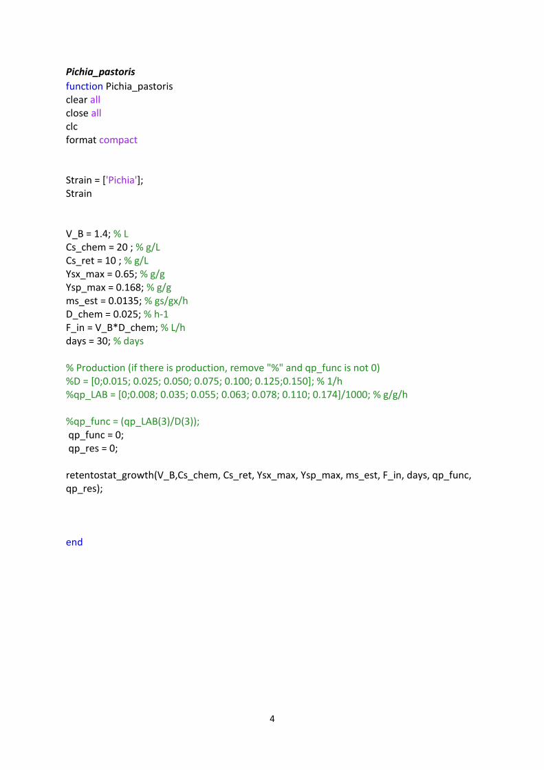
Pichia_pastoris
function Pichia_pastoris clear all close all clc format compact Strain = ['Pichia']; Strain V_B = 1.4; % L Cs_chem = 20 ; % g/L Cs_ret = 10 ; % g/L Ysx_max = 0.65; % g/g Ysp_max = 0.168; % g/g ms_est = 0.0135; % gs/gx/h D_chem = 0.025; % h-1 F_in = V_B*D_chem; % L/h days = 30; % days % Production (if there is production, remove "%" and qp_func is not 0) %D = [0;0.015; 0.025; 0.050; 0.075; 0.100; 0.125;0.150]; % 1/h %qp_LAB = [0;0.008; 0.035; 0.055; 0.063; 0.078; 0.110; 0.174]/1000; % g/g/h %qp_func = (qp_LAB(3)/D(3)); qp_func = 0; qp_res = 0; retentostat_growth(V_B,Cs_chem, Cs_ret, Ysx_max, Ysp_max, ms_est, F_in, days, qp_func, qp_res); end
5
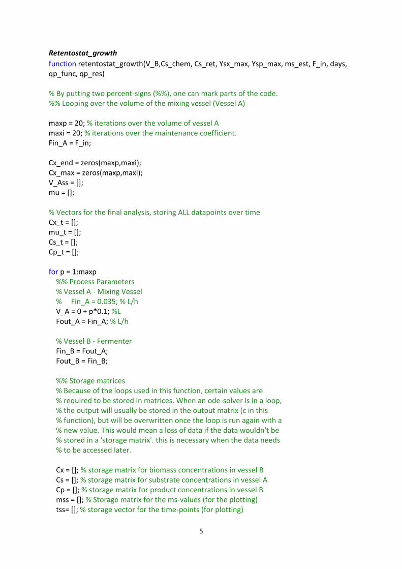
Retentostat_growth
function retentostat_growth(V_B,Cs_chem, Cs_ret, Ysx_max, Ysp_max, ms_est, F_in, days, qp_func, qp_res) % By putting two percent-signs (%%), one can mark parts of the code. %% Looping over the volume of the mixing vessel (Vessel A) maxp = 20; % iterations over the volume of vessel A maxi = 20; % iterations over the maintenance coefficient. Fin_A = F_in; Cx_end = zeros(maxp,maxi); Cx_max = zeros(maxp,maxi); V_Ass = []; mu = []; % Vectors for the final analysis, storing ALL datapoints over time Cx_t = []; mu_t = []; Cs_t = []; Cp_t = []; for p = 1:maxp %% Process Parameters % Vessel A - Mixing Vessel % Fin_A = 0.035; % L/h V_A = 0 + p*0.1; %L Fout_A = Fin_A; % L/h % Vessel B - Fermenter Fin_B = Fout_A; Fout_B = Fin_B; %% Storage matrices % Because of the loops used in this function, certain values are % required to be stored in matrices. When an ode-solver is in a loop, % the output will usually be stored in the output matrix (c in this % function), but will be overwritten once the loop is run again with a % new value. This would mean a loss of data if the data wouldn't be % stored in a 'storage matrix'. this is necessary when the data needs % to be accessed later. Cx = []; % storage matrix for biomass concentrations in vessel B Cs = []; % storage matrix for substrate concentrations in vessel A Cp = []; % storage matrix for product concentrations in vessel B mss = []; % Storage matrix for the ms-values (for the plotting) tss= []; % storage vector for the time-points (for plotting)

6
%% Time span of the ode-solver in h tini= 0 ; % h tend= 24*days; % h dt = 0.5; % the time steps that are used for the ode solver, [h] %% Initial concentrations for the ode-solver % In this model, these are the values that are obtained from the % chemostat phase. The time of 0 hours is when the chemostat is % switched to a retentostat. C_S0 = Cs_chem; % g/L Substrate in the inflow of vessel A %% Looping over ms % Herbert Pirt Equation Parameters for product formation A = qp_func; B = (Ysp_max+Ysx_max*A)/(Ysx_max*Ysp_max); G = qp_res/Ysp_max; for i = 1:maxi ms = (ms_est-maxi/2*0.0001) + i*0.0001 % maintenance coefficient % gs/gx/h C_X0 = ((Fin_B/V_B)*C_S0)/(((Fin_B/V_B)*B)+ms + G); C_P0 = (A*(Fin_B/V_B)+qp_res)*C_X0*V_B/Fout_B; c0 = [C_X0 C_S0 C_P0];% C_SB0]; %% ode solver opt = odeset('RelTol',1e-8, 'AbsTol',1e-8); [t,c] = ode45(@(t,c)dcdt(t,c,ms,Ysx_max,Ysp_max,Cs_ret,F_in,V_A,V_B, qp_res, B, A, G), tini:dt:tend, c0, opt); % there are several ode solvers available. ode45 is most common to % use for 'simple' problems % In order to keep the data available outside of the loop, the concentrations that are % yielded from the ode solver, they are stored in the % storage-matrices as defined above. Cx = [Cx c(:,1)]; Cx_t = [Cx_t c(:,1)]; Cs = [Cs c(:,2)]; Cs_t = [Cs_t c(:,2)]; Cp = [Cp c(:,3)]; Cp_t = [Cp_t c(:,3)]; Cs_B = 0; %% Plotting & Data Handling
7
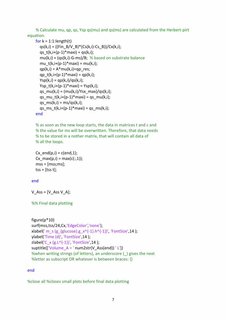
% Calculate mu, qp, qs, Ysp qs(mu) and qs(ms) are calculated from the Herbert-pirt equation. for k = 1:1:length(t) qs(k,i) = ((Fin_B/V_B)*(Cs(k,i)-Cs_B))/Cx(k,i); qs_t(k,i+(p-1)*maxi) = qs(k,i); mu(k,i) = (qs(k,i)-G-ms)/B; % based on substrate balance mu_t(k,i+(p-1)*maxi) = mu(k,i); qp(k,i) = A*mu(k,i)+qp_res; qp_t(k,i+(p-1)*maxi) = qp(k,i); Ysp(k,i) = qp(k,i)/qs(k,i); Ysp_t(k,i+(p-1)*maxi) = Ysp(k,i); qs_mu(k,i) = (mu(k,i)/Ysx_max)/qs(k,i); qs_mu_t(k,i+(p-1)*maxi) = qs_mu(k,i); qs_ms(k,i) = ms/qs(k,i); qs_ms_t(k,i+(p-1)*maxi) = qs_ms(k,i); end % as soon as the new loop starts, the data in matrices t and c and % the value for ms will be overwritten. Therefore, that data needs % to be stored in a nother matrix, that will contain all data of % all the loops. Cx_end(p,i) = c(end,1); Cx_max(p,i) = max(c(:,1)); mss = [mss;ms]; tss = [tss t]; end V_Ass = [V_Ass V_A]; %% Final data plotting figure(p*10) surf(mss,tss/24,Cx,'EdgeColor','none'); xlabel(' m_s (g_{glucose}.g_x^{-1}.h^{-1})', 'FontSize',14 ); ylabel('Time (d)', 'FontSize',14 ); zlabel('C_x (g.L^{-1})', 'FontSize',14 ); suptitle(['Volume_A = ' num2str(V_Ass(end)) ' L']) %when writing strings (of letters), an underscore (_) gives the next %letter as subscript OR whatever is between braces: {} end %close all %closes small plots before final data plotting

8
%% Function Final Output % The function should give the required answers on maximal volume of vessel A for maximal ms % values as written output in the command window. to give written output, % the commands fprintf are used. The constraint on Volume of vessel A is % defined by the maximal volume for which the biomass specific growth rate % remains non-negative (= starvation). Cx_eval = Cx_max./Cx_end; % evaluate whether Cx max is at the end of the % retentostat mu_thres = ones(length(t),1)*1e-3; % This vector is created to have a % threshold line for the growth rate (has to be below 0.001 h-1 for p = 1:maxp; if Cx_eval(p,maxi) > 1 % It is easiest to have the output in an easily accessible format, % here a sentence. fprintf(['The maximal volume of mixing vessel A for ' ... 'which a robust set-up can be guaranteed \n based on this model, ' ... 'up to an ms of ' num2str(mss(maxi)) ' is a volume of '... num2str(V_Ass(p-1)) ' L. \n' ]) % It has to be p-1, because if p is used for the volume, the Cx_eval % is already > 1. % but a visual check of the conclusion is required as well. for a = 0:1 % plot for the first 'wrong' V_A and the last ' good' V_A. figure((p-a)*101);% suptitle(['Volume_A = ' num2str(V_Ass(p-a)) ' L']) Fontsize = 15; % Biomass concentration subplot(3,3,1) plot(t/24,Cx_t(:,1+((p-a)-1)*maxi),'r',t/24,Cx_t(:,(maxi+((p-a)-1)*maxi)),'k-', 'LineWidth', 1.5); hold on; xlabel(' Time (d)', 'FontSize',15 ); ylabel('C_x (g.L^{-1})', 'FontSize',15 ); title('a','FontSize',Fontsize); % Specific growth rate subplot(3,3,4) plot(t/24,mu_t(:,1+((p-a)-1)*maxi),'r',t/24,mu_t(:,maxi+((p-a)-1)*maxi),'k-', 'LineWidth', 1.5); hold on; xlabel(' Time (d)', 'FontSize',15 ); ylabel('\mu (h^{-1})', 'FontSize',15 ); title('d','FontSize',Fontsize); % Substrate inflow concentration subplot(3,3,2)
9
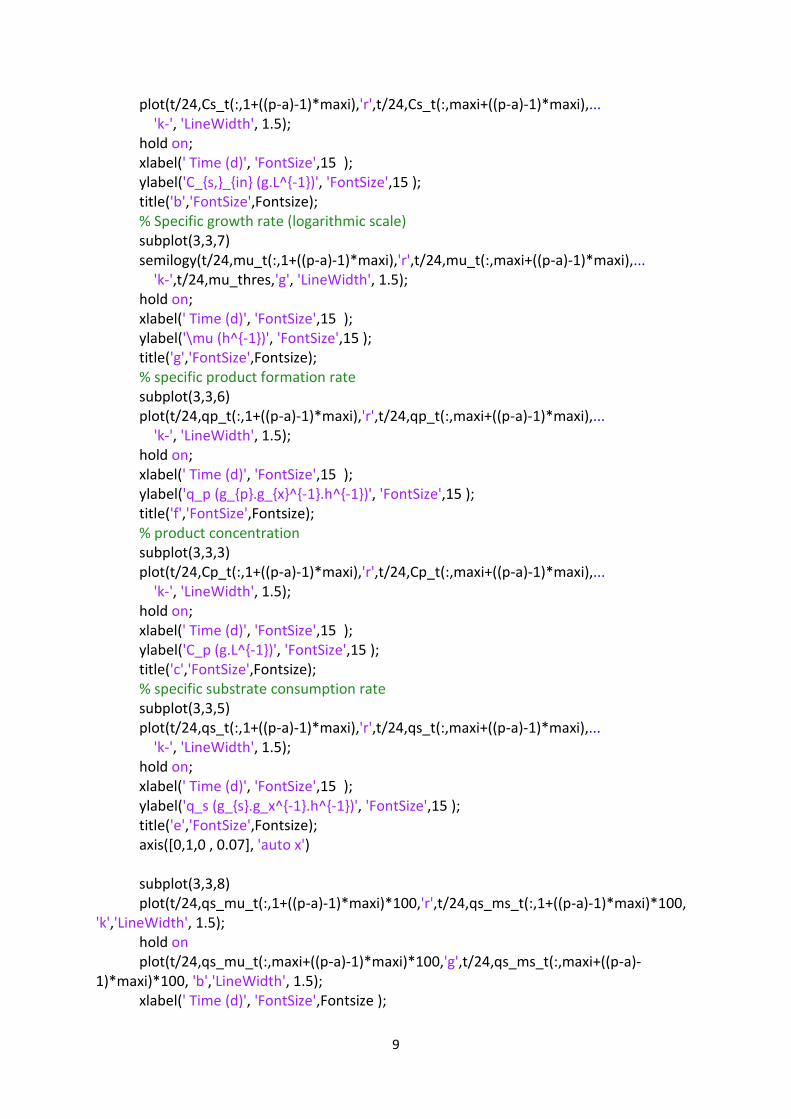
plot(t/24,Cs_t(:,1+((p-a)-1)*maxi),'r',t/24,Cs_t(:,maxi+((p-a)-1)*maxi),... 'k-', 'LineWidth', 1.5); hold on; xlabel(' Time (d)', 'FontSize',15 ); ylabel('C_{s,}_{in} (g.L^{-1})', 'FontSize',15 ); title('b','FontSize',Fontsize); % Specific growth rate (logarithmic scale) subplot(3,3,7) semilogy(t/24,mu_t(:,1+((p-a)-1)*maxi),'r',t/24,mu_t(:,maxi+((p-a)-1)*maxi),... 'k-',t/24,mu_thres,'g', 'LineWidth', 1.5); hold on; xlabel(' Time (d)', 'FontSize',15 ); ylabel('\mu (h^{-1})', 'FontSize',15 ); title('g','FontSize',Fontsize); % specific product formation rate subplot(3,3,6) plot(t/24,qp_t(:,1+((p-a)-1)*maxi),'r',t/24,qp_t(:,maxi+((p-a)-1)*maxi),... 'k-', 'LineWidth', 1.5); hold on; xlabel(' Time (d)', 'FontSize',15 ); ylabel('q_p (g_{p}.g_{x}^{-1}.h^{-1})', 'FontSize',15 ); title('f','FontSize',Fontsize); % product concentration subplot(3,3,3) plot(t/24,Cp_t(:,1+((p-a)-1)*maxi),'r',t/24,Cp_t(:,maxi+((p-a)-1)*maxi),... 'k-', 'LineWidth', 1.5); hold on; xlabel(' Time (d)', 'FontSize',15 ); ylabel('C_p (g.L^{-1})', 'FontSize',15 ); title('c','FontSize',Fontsize); % specific substrate consumption rate subplot(3,3,5) plot(t/24,qs_t(:,1+((p-a)-1)*maxi),'r',t/24,qs_t(:,maxi+((p-a)-1)*maxi),... 'k-', 'LineWidth', 1.5); hold on; xlabel(' Time (d)', 'FontSize',15 ); ylabel('q_s (g_{s}.g_x^{-1}.h^{-1})', 'FontSize',15 ); title('e','FontSize',Fontsize); axis([0,1,0 , 0.07], 'auto x') subplot(3,3,8) plot(t/24,qs_mu_t(:,1+((p-a)-1)*maxi)*100,'r',t/24,qs_ms_t(:,1+((p-a)-1)*maxi)*100, 'k','LineWidth', 1.5); hold on plot(t/24,qs_mu_t(:,maxi+((p-a)-1)*maxi)*100,'g',t/24,qs_ms_t(:,maxi+((p-a)-1)*maxi)*100, 'b','LineWidth', 1.5); xlabel(' Time (d)', 'FontSize',Fontsize );

10
ylabel('Gluc. distr. (%)', 'FontSize',Fontsize ); title('h','FontSize',Fontsize ); % Product on substrate yield subplot(3,3,9) plot(t/24,Ysp_t(:,1+((p-a)-1)*maxi),'r',t/24,Ysp_t(:,maxi+((p-a)-1)*maxi),... 'k-', 'LineWidth', 1.5); hold on; xlabel(' Time (d)', 'FontSize',15 ); ylabel('Y_{sp} (g_p.g_s^{-1})', 'FontSize',15 ); title('i','FontSize',Fontsize); end break end end end function dc = dcdt(t,c,ms,Ysx_max,Ysp_max,Cs_ret,F_in,V_A,V_B, qp_res, B, A, G) % global Fin_A V_A Fout_A ms Ysx_max Ysp_max qp V_B %% Variables Cx_B = c(1); Cs_A = c(2); Cp_B = c(3); Cs_B = 0; %% Model Parameters % Vessel A - Mixing Vessel Cs_R = Cs_ret; % the concentration in the second medium vessel; eventually the concentration in vessel A. % Vessel B - Fermentor Fin_A = F_in; Fout_A = Fin_A; Fin_B = Fout_A; Fout_B = Fin_B;

11
qs = ((Fin_B/V_B)*(Cs_A-Cs_B))/Cx_B; mu = (qs - G - ms)/B; qp = A * mu + qp_res; %% Equations dc(1) = mu*Cx_B; % Balance of Cx_B dc(2) = Fin_A/V_A*Cs_R - Fout_A/V_A*Cs_A; % % Balance of Cs_A dc(3) = qp*Cx_B-Fout_B*Cp_B; % Balance of Cp_B: Product formation dc = dc'; end
12
HOW TO – MATLAB regression model
For the non-linear regression analysis the MATLAB codes Example_rententostat_data,
Retentostat_regression_Pp_kd and_plotting (see below) as well as the Excel supplemental
file 2 (Example_retentostat_data.xlsx) are required. The MATLAB codes need to be
converted into separate MATLAB files. Together, these documents allow to perform a
regression analysis on experimental data from retentostat cultures, and have to be kept in
the same folder to function properly.
Excel sheet MATLABread in the file Example_retentostat_data.xlsx, contains data collected
from an example retentostat experiment. In this sheet are incorporated the (viable) biomass
concentration and the glucose concentration in the feed. The different volumes and flow
rates taken into account by the model are indicated in the data sheet as well.
Example_rententostat_data is the MATLAB code that has to be run in MATLAB to do a
regression analysis. When executed, it automatically requests data from Sheet MATLABread
in the file Example_retentostat_data.xlsx, and calls for the function in the code
Retentostat_regression_Pp_kd. The function in the latter contain the ordinary differential
equations (ODEs) that are needed to describe (viable and total) biomass accumulation in the
retentostat (see Materials and Methods), which are solved multiple times for varying values
of mS (maintenance energy requirements mS), and kd (death rate kd) until the sum of square
errors (SSE) is minimized.
Data is plotted using the code retentostat_plotting.
Sheet Modelling Summary in the Excel file Example_retentostat_data.xlsx is where MATLAB
deposits the data after a complete regression analysis. In here, ms opt is the value for mS (in
mg·g-1·h-1) corresponding to the regression with the lowest SSE. In addition, values for SSE,
r-squared (Rsq), optimised death rate (Kd [“value”·10-3 h-1]) and the final specific growth
rate at the end of retentostat (in h-1). Furthermore, the glucose concentration in the feed
(Cs), the biomass concentration in the retentostat (Cx) the specific growth rate (mu) and the
specific substrate uptake rate (qs) are published according to the regression analysis, with a
step size of 30 minutes.
To personalize the files for new retentostat experiments with other organisms or different
conditions, one can change the following values, arranged according to the files they appear
in:

13
Code Example_rententostat_data.xlsx
Change all data in sheet MATLABread according to your personal experimental data
Sheet Modelling Summary is automatically emptied and filled with each new
regression analysis.
Code Example_rententostat_data
Yeast parameters (qp and Ysp_max refers to production characteristics of a strain*)
The data location that is read by MATLAB from an Excel file (filename =
'Example_retentostat_data.xlsx').
File Retentostat_regression_Pp_kd
Initial guesses for ms and kd (in gglucose·gbiomass-1·h-1 and in h-1, respectively), starting
point for solving ODEs and minimizing SSE.
Time span of retentostat (in days)
Concentration in the medium reservoir during retentostat
*Optional product terms: for linear qp (mu)-relations (qp = a*mu+b), qp_func = parameter a
and qp_res = parameter b, with qp [g·gX-1·h-1] and Ysp_max in [gP·gS
-1]. For non-producing
strains qp terms equal 0.
14
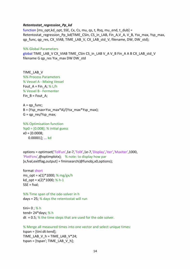
Retentostat_regression_Pp_kd
function [ms_opt,kd_opt, SSE, Cx, Cs, mu, qs, t, Rsq, mu_end, t_dub] = Retentostat_regression_Pp_kd(TIME_CSin, CS_in_LAB, Fin_A,V_A, V_B, Ysx_max, Ysp_max, qp_func, qp_res, CX_VIAB, TIME_LAB_V, CX_LAB_std_V, filename, DW, DW_std); %% Global Parameters global TIME_LAB_V CX_VIAB TIME_CSin CS_in_LAB V_A V_B Fin_A A B CX_LAB_std_V filename G qp_res Ysx_max DW DW_std TIME_LAB_V %% Process Parameters % Vessel A - Mixing Vessel Fout_A = Fin_A; % L/h % Vessel B - Fermenter Fin_B = Fout_A; A = qp_func; B = (Ysp_max+Ysx_max*A)/(Ysx_max*Ysp_max); G = qp_res/Ysp_max; %% Optimisation function %p0 = [0.008]; % initial guess x0 = [0.0008; 0.00001]; ... kd options = optimset('TolFun',1e-7,'TolX',1e-7,'Display','iter','MaxIter',1000, 'PlotFcns',@optimplotx); % note: to display how par [x,fval,exitflag,output] = fminsearch(@funobj,x0,options); format short ms_opt = x(1)*1000; % mg/gx/h kd_opt = x(2)*1000; % h-1 SSE = fval; %% Time span of the ode-solver in h days = 25; % days the retentostat will run tini= 0 ; % h tend= 24*days; % h dt = 0.5; % the time steps that are used for the ode solver. % Merge all measured times into one vector and select unique times: tspan = [tini:dt:tend]; TIME_LAB_V_h = TIME_LAB_V*24; tspan = [tspan'; TIME_LAB_V_h];
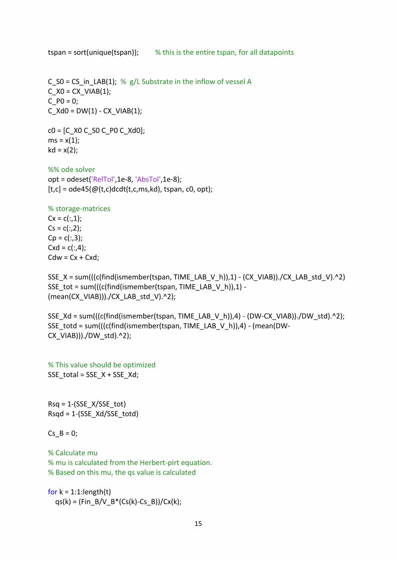
15
tspan = sort(unique(tspan)); % this is the entire tspan, for all datapoints C_S0 = CS_in_LAB(1); % g/L Substrate in the inflow of vessel A C_X0 = CX_VIAB(1); C_P0 = 0; C_Xd0 = DW(1) - CX_VIAB(1); c0 = [C_X0 C_S0 C_P0 C_Xd0]; ms = x(1); kd = x(2); %% ode solver opt = odeset('RelTol',1e-8, 'AbsTol',1e-8); [t,c] = ode45(@(t,c)dcdt(t,c,ms,kd), tspan, c0, opt); % storage-matrices Cx = c(:,1); Cs = c(:,2); Cp = c(:,3); Cxd = c(:,4); Cdw = Cx + Cxd; SSE_X = sum(((c(find(ismember(tspan, TIME_LAB_V_h)),1) - (CX_VIAB))./CX_LAB_std_V).^2) SSE_tot = sum(((c(find(ismember(tspan, TIME_LAB_V_h)),1) - (mean(CX_VIAB)))./CX_LAB_std_V).^2); SSE_Xd = sum(((c(find(ismember(tspan, TIME_LAB_V_h)),4) - (DW-CX_VIAB))./DW_std).^2); SSE_totd = sum(((c(find(ismember(tspan, TIME_LAB_V_h)),4) - (mean(DW-CX_VIAB)))./DW_std).^2); % This value should be optimized SSE_total = SSE_X + SSE_Xd; Rsq = 1-(SSE_X/SSE_tot) Rsqd = 1-(SSE_Xd/SSE_totd) Cs_B = 0; % Calculate mu % mu is calculated from the Herbert-pirt equation. % Based on this mu, the qs value is calculated for k = 1:1:length(t) qs(k) = (Fin_B/V_B*(Cs(k)-Cs_B))/Cx(k);
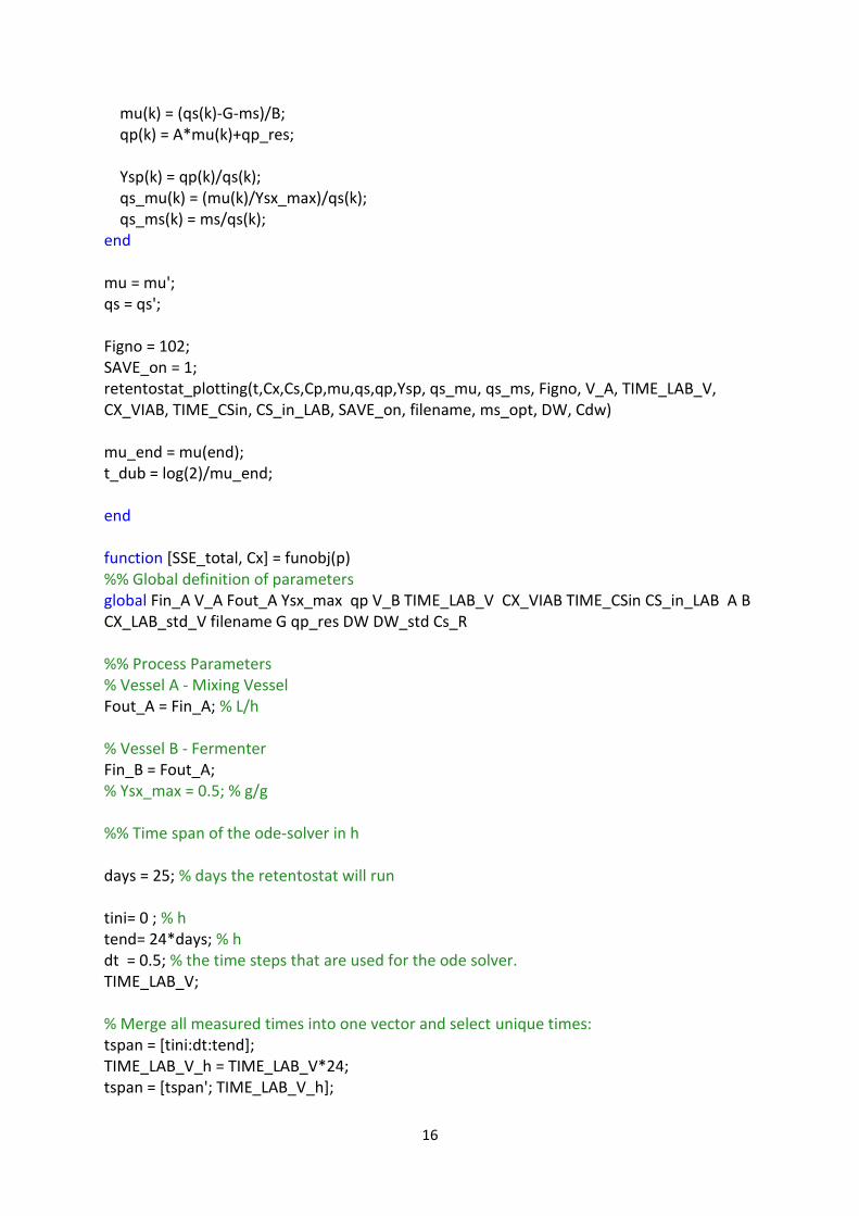
16
mu(k) = (qs(k)-G-ms)/B; qp(k) = A*mu(k)+qp_res; Ysp(k) = qp(k)/qs(k); qs_mu(k) = (mu(k)/Ysx_max)/qs(k); qs_ms(k) = ms/qs(k); end mu = mu'; qs = qs'; Figno = 102; SAVE_on = 1; retentostat_plotting(t,Cx,Cs,Cp,mu,qs,qp,Ysp, qs_mu, qs_ms, Figno, V_A, TIME_LAB_V, CX_VIAB, TIME_CSin, CS_in_LAB, SAVE_on, filename, ms_opt, DW, Cdw) mu_end = mu(end); t_dub = log(2)/mu_end; end function [SSE_total, Cx] = funobj(p) %% Global definition of parameters global Fin_A V_A Fout_A Ysx_max qp V_B TIME_LAB_V CX_VIAB TIME_CSin CS_in_LAB A B CX_LAB_std_V filename G qp_res DW DW_std Cs_R %% Process Parameters % Vessel A - Mixing Vessel Fout_A = Fin_A; % L/h % Vessel B - Fermenter Fin_B = Fout_A; % Ysx_max = 0.5; % g/g %% Time span of the ode-solver in h days = 25; % days the retentostat will run tini= 0 ; % h tend= 24*days; % h dt = 0.5; % the time steps that are used for the ode solver. TIME_LAB_V; % Merge all measured times into one vector and select unique times: tspan = [tini:dt:tend]; TIME_LAB_V_h = TIME_LAB_V*24; tspan = [tspan'; TIME_LAB_V_h];

17
tspan = sort(unique(tspan)); % this is the entire tspan, for all datapoints %% Initial concentrations for the ode-solver % In this model, these are the values that are obtained from the % chemostat phase, where we know there is a steady state. The time of 0 hours is when the chemostat is % switched to a retentostat. C_S0 = CS_in_LAB(1); % g/L Substrate in the inflow of vessel A C_P0 = 0; % g/L Product in the outflow of vessel B C_Xd0 = 0; ms = p(1); % maintenance coefficient % gs/gx/h kd = p(2); C_X0 = CX_VIAB(1); C_Xd0 = DW(1)-CX_VIAB(1); c0 = [C_X0 C_S0 C_P0 C_Xd0]; Cs_R = CS_in_LAB(end); %% ode solver opt = odeset('RelTol',1e-8, 'AbsTol',1e-8); [t,c] = ode45(@(t,c)dcdt(t,c,ms,kd, Cs_R), tspan, c0, opt); % storage-matrices Cx = c(:,1); Cs = c(:,2); Cp = c(:,3); Cxd = c(:,4); Cdw = Cx + Cxd; %% Plotting & Data Handling % Calculate mu % mu is calculated from the Herbert-pirt equation. % Based on this mu, the qs, qp and Ysp values are calculated Cs_B = 0; for k = 1:length(t) qs(k) = (Fin_B/V_B*(Cs(k)-Cs_B))/Cx(k); mu(k) = (qs(k)-G-ms)/B; qp(k) = A*mu(k)+qp_res; Ysp(k) = qp(k)/qs(k); qs_mu(k) = (mu(k)/Ysx_max)/qs(k); qs_ms(k) = ms/qs(k); end

18
%% Final data plotting %% Function Final Output % Select ODE values for the right tspan values and calculate sum of squares % format long c(find(ismember(tspan, TIME_LAB_V_h)),1) (CX_VIAB)./CX_LAB_std_V SSE_X = sum(((c(find(ismember(tspan, TIME_LAB_V_h)),1) - (CX_VIAB))./CX_LAB_std_V).^2) SSE_tot = sum(((c(find(ismember(tspan, TIME_LAB_V_h)),1) - (mean(CX_VIAB)))./CX_LAB_std_V).^2) SSE_Xd = sum(((c(find(ismember(tspan, TIME_LAB_V_h)),4) - (DW-CX_VIAB))./DW_std).^2) SSE_totd = sum(((c(find(ismember(tspan, TIME_LAB_V_h)),4) - (mean(DW-CX_VIAB)))./DW_std).^2) R2v = 1-(SSE_X/SSE_tot); R2d = 1-(SSE_Xd/SSE_totd); % This value should be optimized SSE_total = SSE_X + SSE_Xd; Figno = 101; SAVE_on = 0; %retentostat_plotting(t,Cx,Cs,Cp,mu,qs,qp,Ysp, qs_mu, qs_ms, Figno, V_A, TIME_LAB_V, CX_VIAB, TIME_CSin, CS_in_LAB, SAVE_on, filename, ms*1000, DW, Cdw) end function dc = dcdt(t,c,ms,kd, Cs_R) global Fin_A V_A V_B A B G qp_res %% Variables Cx_B = c(1); Cs_A = c(2); Cp_B = c(3); Cxd_B = c(4); Cs_B = 0; %% Model Parameters % Vessel A - Mixing Vessel Cs_R = 5; % the concentration in the second medium vessel; eventually the concentration in vessel A.

19
% Vessel B - Fermentor Fout_A = Fin_A; Fin_B = Fout_A; Fout_B = Fin_B; qs = ((Fin_B/V_B)*(Cs_A-Cs_B))/Cx_B; mu = (qs - G - ms)/B; qp = A * mu + qp_res; %% Equations dc(1) = mu*Cx_B - kd*Cx_B; % Balance of Cx_B dc(2) = Fin_A/V_A*Cs_R - Fout_A/V_A*Cs_A; % % Balance of Cs_A dc(3) = qp*Cx_B-Fout_B*Cp_B; % Balance of Cp_B: Product formation dc(4) = kd * Cx_B; % balance of dead biomass dc = dc'; end
20
Retentostat_plotting
function retentostat_plotting(t,Cx,Cs,Cp,mu,qs,qp,Ysp, qs_mu, qs_ms, Figno, V_A, TIME_LAB_V, CX_VIAB, TIME_CSin, CS_in_LAB, SAVE_on, filename, ms, DW, Cdw) h = figure(Figno); if SAVE_on == 0 suptitle(['Volume_A = ' num2str(V_A) ' L, ms = ' num2str(ms) ' mg/gx/h ' ]) end Fontsize = 13; Linewidth = 1; subplot(3,3,1) plot(t/24,Cx(:,1),'k-.', 'LineWidth', Linewidth); hold on; plot(t/24,Cdw(:,1), 'r-.', 'LineWidth', Linewidth); hold on xlabel(' Time (d)', 'FontSize',Fontsize ); ylabel('C_x (g.L^{-1})', 'FontSize',Fontsize ); hold on; plot(TIME_LAB_V, CX_VIAB,'m.','LineWidth',Linewidth); hold on plot(TIME_LAB_V, DW,'g.', 'LineWidth', Linewidth); title('a','FontSize',Fontsize ); axis([0,25,0 , 1], 'auto y') subplot(3,3,2) plot(t/24,Cs,'k-.', 'LineWidth', Linewidth); hold on; xlabel(' Time (d)', 'FontSize',Fontsize ); ylabel('C_{s,}_{in} (g.L^{-1})', 'FontSize',Fontsize ); plot(TIME_CSin, CS_in_LAB,'.') title('b','FontSize',Fontsize ); axis([0,25,0 , 1], 'auto y') subplot(3,3,3) plot(t/24,Cp, 'k','LineWidth', Linewidth); xlabel(' Time (d)', 'FontSize',Fontsize ); ylabel('C_p (g_{p}.L^{-1})', 'FontSize',Fontsize ); title('c','FontSize',Fontsize ); axis([0,25,0 , 1], 'auto y') subplot(3,3,4) plot(t/24,mu,'k-.', 'LineWidth', Linewidth); hold on; xlabel(' Time (d)', 'FontSize',Fontsize ); ylabel('\mu (h^{-1})', 'FontSize',Fontsize );

21
title('d','FontSize',Fontsize ); axis([0,25,0 , 1], 'auto y') subplot(3,3,5) plot(t/24,qs, 'k','LineWidth', Linewidth); hold on plot(t/24,ones(length(t))*ms/1000,'g', 'LineWidth',Linewidth); xlabel(' Time (d)', 'FontSize',Fontsize ); ylabel('q_s (g_{s}.g_x^{-1}.h^{-1})', 'FontSize',Fontsize ); title('e','FontSize',Fontsize ); axis([0,25,0 , 1], 'auto y') subplot(3,3,6) plot(t/24,qp, 'k','LineWidth', Linewidth); xlabel(' Time (d)', 'FontSize',Fontsize ); ylabel('q_p (g_{p}.g_x^{-1}.h^{-1})', 'FontSize',Fontsize ); title('f','FontSize',Fontsize ); axis([0,25,0 , 1], 'auto y') subplot(3,3,7) semilogy(t/24,mu,'m', 'LineWidth', Linewidth); hold on; xlabel(' Time (d)', 'FontSize',Fontsize ); ylabel('\mu (h^{-1})', 'FontSize',Fontsize ); title('g','FontSize',Fontsize ); axis([0,25,0 , 1], 'auto y') subplot(3,3,8) plot(t/24,qs_mu*100,t/24,qs_ms*100, 'k','LineWidth', Linewidth); xlabel(' Time (d)', 'FontSize',Fontsize ); ylabel('Gluc. distr. (%)', 'FontSize',Fontsize ); title('h','FontSize',Fontsize ); axis([0,25,0 , 1], 'auto y') subplot(3,3,9) plot(t/24,Ysp, 'k','LineWidth', Linewidth); xlabel(' Time (d)', 'FontSize',Fontsize ); ylabel('Y_{sp} (g_{p}.g_{s}^{-1})', 'FontSize',Fontsize ); title('i','FontSize',Fontsize ); axis([0,25,0 , 1], 'auto y') if SAVE_on == 1 saveas(h,[num2str(date) num2str(filename(1:end-4)) '_final_plot'],'m') end end
22
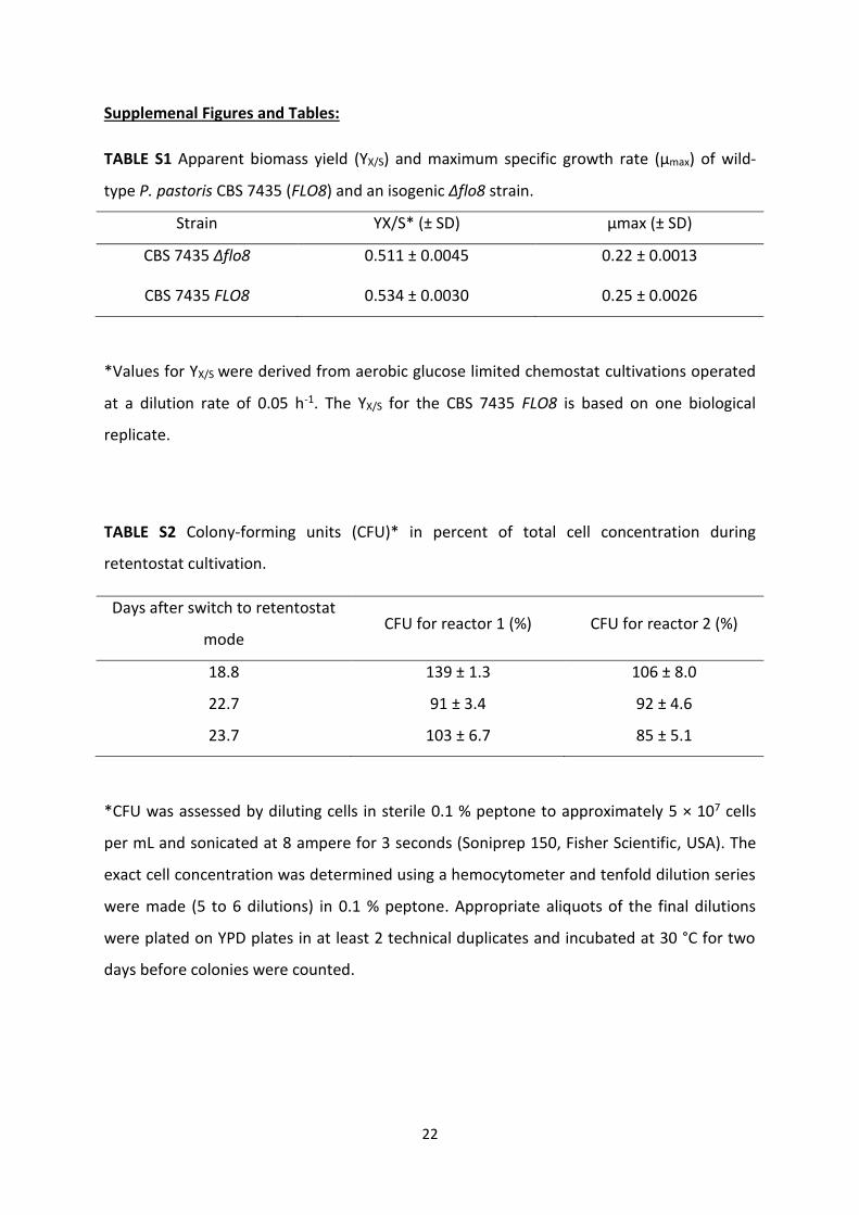
Supplemenal Figures and Tables:
TABLE S1 Apparent biomass yield (YX/S) and maximum specific growth rate (µmax) of wild-
type P. pastoris CBS 7435 (FLO8) and an isogenic ∆flo8 strain.
Strain YX/S* (± SD) µmax (± SD)
CBS 7435 ∆flo8 0.511 ± 0.0045 0.22 ± 0.0013
CBS 7435 FLO8 0.534 ± 0.0030 0.25 ± 0.0026
*Values for YX/S were derived from aerobic glucose limited chemostat cultivations operated
at a dilution rate of 0.05 h-1. The YX/S for the CBS 7435 FLO8 is based on one biological
replicate.
TABLE S2 Colony-forming units (CFU)* in percent of total cell concentration during
retentostat cultivation.
Days after switch to retentostat
mode CFU for reactor 1 (%) CFU for reactor 2 (%)
18.8 139 ± 1.3 106 ± 8.0
22.7 91 ± 3.4 92 ± 4.6
23.7 103 ± 6.7 85 ± 5.1
*CFU was assessed by diluting cells in sterile 0.1 % peptone to approximately 5 × 10⁷ cells
per mL and sonicated at 8 ampere for 3 seconds (Soniprep 150, Fisher Scientific, USA). The
exact cell concentration was determined using a hemocytometer and tenfold dilution series
were made (5 to 6 dilutions) in 0.1 % peptone. Appropriate aliquots of the final dilutions
were plated on YPD plates in at least 2 technical duplicates and incubated at 30 °C for two
days before colonies were counted.

23
FIG S1 Regression analysis on overlapping sets of specific growth rate versus glucose uptake
rate relations (µ - qS) from 4 data points measured at different consecutive specific growth
rates (see Materials and Methods). Values for the maintenance coefficient (mS) and the
maximum yield on biomass (YX/Smax) were calculated from plots qS1 - qS7 which resulted in a
24
R2 of at least 0.99. Linear regression on data represented in plots qS8 - qS10 resulted in R2
values below 0.99 and were not considered further to assess the growth rate dependency of
mS and YX/Smax as depicted in Fig 6 in the manuscript.
25
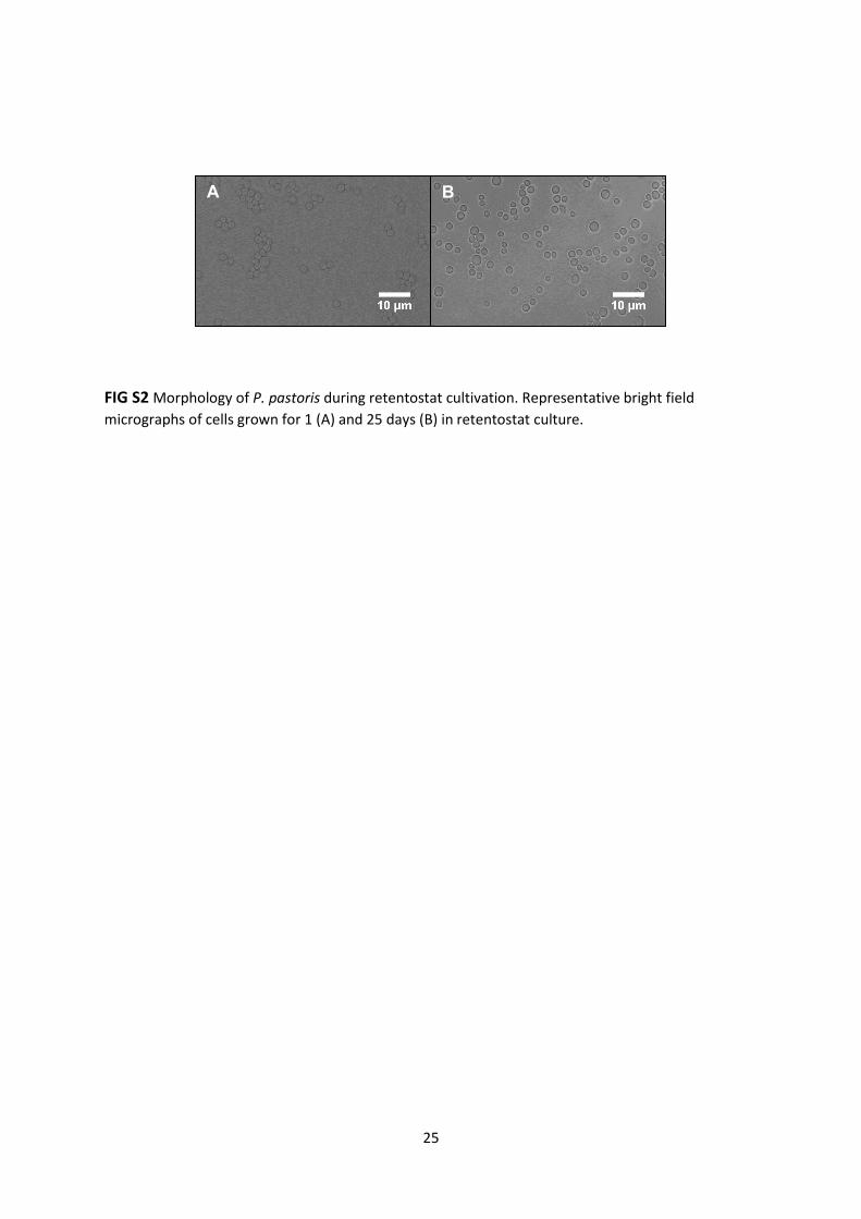
FIG S2 Morphology of P. pastoris during retentostat cultivation. Representative bright field
micrographs of cells grown for 1 (A) and 25 days (B) in retentostat culture.
A B

26
Tim e in retentostat [days]
0 5 10 15 20 25 30
Bio
ma
ss
[g
L-1
]
0
10
20
30
40
qS [
gS g
X
-1 h
-1],
µ [
h-1
]
0.0001
0.001
0.01
0.1
FIG S3 Example of non-linear regression analysis of viable biomass for one retentostat.
Viable biomass (closed circles), non-linear regression of viable biomass (short dashed line)
and resulting glucose uptake rate (qS, long dashed line) as well as specific growth rate (µ,
solid line).