Supplement#6s - summary
31
SUPPLEMENT OUTLINE Introduction, 2 Linear Programming Models, 2 Model Formulation, 4 Graphical Linear Programming, 5 Outline of Graphical Procedure, 5 Plotting Constraints, 7 Identifying the Feasible Solution Space, 10 Plotting the Objective Function Line, 7 Redundant Constraints, 14 Solutions and Corner Points, 14 Minimization, 15 Slack and Surplus, 17 The Simplex Method, 17 Computer Solutions, 17 Solving LP Models Using MS Excel, 18 Sensitivity Analysis, 20 Objective Function Coefficient Changes, 21 Changes in the Right-Hand Side Value of a Constraint, 22 Key Terms, 24 Solved Problems, 24 Discussion and Review Questions, 26 Problems, 26 Case: Son, Ltd., 31 Selected Bibliography and Further Reading, 31 LEARNING OBJECTIVES After completing this supplement, you should be able to: 1 Describe the type of problem that would lend itself to solution using linear programming. 2 Formulate a linear programming model from a description of a problem. 3 Solve simple linear programming problems using the graphical method. 4 Interpret computer solutions of linear programming problems. 5 Do sensitivity analysis on the solution of a linear programming problem. SUPPLEMENT TO CHAPTER SIX Linear Programming 1
-
Upload
advancedaccountant -
Category
Documents
-
view
276 -
download
1
description
This is the summary to the supplemental of the summary supplement
Transcript of Supplement#6s - summary
SUPPLEMENT OUTLINE
Introduction, 2
Linear Programming Models, 2Model Formulation, 4
Graphical Linear Programming, 5Outline of Graphical Procedure, 5Plotting Constraints, 7Identifying the Feasible Solution
Space, 10Plotting the Objective
Function Line, 7Redundant Constraints, 14Solutions and Corner Points, 14Minimization, 15Slack and Surplus, 17
The Simplex Method, 17
Computer Solutions, 17
Solving LP Models Using MS Excel, 18
Sensitivity Analysis, 20Objective Function Coefficient
Changes, 21Changes in the Right-Hand Side
Value of a Constraint, 22
Key Terms, 24
Solved Problems, 24
Discussion and ReviewQuestions, 26
Problems, 26
Case: Son, Ltd., 31
Selected Bibliography and FurtherReading, 31
LEARNING OBJECTIVES
After completing this supplement,you should be able to:
1 Describe the type of problem thatwould lend itself to solution usinglinear programming.
2 Formulate a linear programmingmodel from a description of aproblem.
3 Solve simple linear programmingproblems using the graphicalmethod.
4 Interpret computer solutions oflinear programming problems.
5 Do sensitivity analysis on thesolution of a linear programmingproblem.
SUPPLEMENT TO CHAPTER SIX
Linear Programming
1
chapter6-suppliment.qxd 4/11/03 3:35 PM Page 1
L inear programming is a powerful quantitative tool used by operations managers andother managers to obtain optimal solutions to problems that involve restrictions or
limitations, such as the available materials, budgets, and labour and machine time. Theseproblems are referred to as constrained optimization problems. There are numerousexamples of linear programming applications to such problems, including:
• Establishing locations for emergency equipment and personnel that will minimizeresponse time
• Determining optimal schedules for airlines for planes, pilots, and ground personnel
• Developing financial plans
• Determining optimal blends of animal feed mixes
• Determining optimal diet plans
• Identifying the best set of worker–job assignments
• Developing optimal production schedules
• Developing shipping plans that will minimize shipping costs
• Identifying the optimal mix of products in a factory
IntroductionLinear programming (LP) techniques consist of a sequence of steps that will lead to anoptimal solution to problems, in cases where an optimum exists. There are a number ofdifferent linear programming techniques; some are special-purpose (i.e., used to find solu-tions for specific types of problems) and others are more general in scope. This supplementcovers the two general-purpose solution techniques: graphical linear programming and com-puter solutions. Graphical linear programming provides a visual portrayal of many of theimportant concepts of linear programming. However, it is limited to problems with only twovariables. In practice, computers are used to obtain solutions for problems, some of whichinvolve a large number of variables.
Linear Programming ModelsLinear programming models are mathematical representations of constrained optimizationproblems. These models have certain characteristics in common. Knowledge of these char-acteristics enables us to recognize problems that can be solved using linear programming.In addition, it also can help us formulate LP models. The characteristics can be groupedinto two categories: components and assumptions. First, let’s consider the components.
Four components provide the structure of a linear programming model:
1. Objective.
2. Decision variables.
3. Constraints.
4. Parameters.
Linear programming algorithms require that a single goal or objective, such as the maxi-mization of profits, be specified. The two general types of objectives are maximizationand minimization. A maximization objective might involve profits, revenues, efficiency,or rate of return. Conversely, a minimization objective might involve cost, time, distancetravelled, or scrap. The objective function is a mathematical expression that can be usedto determine the total profit (or cost, etc., depending on the objective) for a given solution.
Decision variables represent choices available to the decision maker in terms ofamounts of either inputs or outputs. For example, some problems require choosing a com-bination of inputs to minimize total costs, while others require selecting a combination ofoutputs to maximize profits or revenues.
2 PART THREE SYSTEM DESIGN
objective function Mathemat-ical statement of profit (or cost,etc.) for a given solution.
decision variables Amountsof either inputs or outputs.
chapter6-suppliment.qxd 4/11/03 3:35 PM Page 2

Constraints are limitations that restrict the alternatives available to decision makers.The three types of constraints are less than or equal to (�), greater than or equal to (�),and simply equal to (�). A � constraint implies an upper limit on the amount of somescarce resource (e.g., machine hours, labour hours, materials) available for use. A � con-straint specifies a minimum that must be achieved in the final solution (e.g., must containat least 10 percent real fruit juice, must get at least 30 km/L on the highway). The � con-straint is more restrictive in the sense that it specifies exactly what a decision variableshould equal (e.g., make 200 units of product A). A linear programming model canconsist of one or more constraints. The constraints of a given problem define the set of allfeasible combinations of decision variables; this set is referred to as the feasible solutionspace. Linear programming algorithms are designed to search the feasible solution spacefor the combination of decision variables that will yield an optimum in terms of theobjective function.
An LP model consists of a mathematical statement of the objective and a mathemati-cal statement of each constraint. These statements consist of symbols (e.g., x1, x2) that rep-resent the decision variables and numerical values, called parameters. The parametersare fixed values; the model is solved given those values.
Example S–1 illustrates the components of an LP model.
x1 � Quantity of product 1 to produceu x2 � Quantity of product 2 to produce
x3 � Quantity of product 3 to produce
Maximize 5x1 � 8x2 � 4x3 (profit) (Objective function)
Subject to
Labour 2x1 � 4x2 � 8x3 � 250 hours
Material 7x1 � 6x2 � 5x3 � 100 kg (Constraints)
Product 1 x1 � 10 units
x1, x2, x3 � 0 (Nonnegativity constraints)
First, the model lists and defines the decision variables. These typically representquantities. In this case, they are quantities of three different products that might beproduced.
Next, the model states the objective function. It includes every decision variable in themodel and the contribution (profit per unit) of each decision variable. Thus, product x1 hasa profit of $5 per unit. The profit from product x1 for a given solution will be 5 times thevalue of x1 specified by the solution; the total profit from all products will be the sum ofthe individual product profits. Thus, if x1 � 10, x2 � 0, and x3 � 6, the value of theobjective function would be:
5(10) � 8(0) � 4(6) � 74
The objective function is followed by a list (in no particular order) of three constraints.Each constraint has a right-side numerical value (e.g., the labour constraint has a right-side value of 250) that indicates the amount of the constraint and a relation sign that indi-cates whether that amount is a maximum (�), a minimum (�), or an equality (�). Theleft side of each constraint consists of the variables subject to that particular constraint anda coefficient for each variable that indicates how much of the right-side quantity one unitof the decision variable represents. For instance, for the labour constraint, one unit of x1
will require two hours of labour. The sum of the values on the left side of each constraintrepresents the amount of that constraint used by a solution. Thus, if x1 � 10, x2 � 0, and x3 � 6, the amount of labour used would be:
2(10) � 4(0) � 8(6) � 68 hours
Decision variables
SUPPLEMENT TO CHAPTER SIX LINEAR PROGRAMMING 3
constraints Limitations thatrestrict the availablealternatives.
feasible solution space Theset of all feasible combinationsof decision variables as definedby the constraints.
parameters Numericalconstants.
Example S–1
chapter6-suppliment.qxd 4/11/03 3:35 PM Page 3

Because this amount does not exceed the quantity on the right-hand side of the constraint,it is feasible.
Note that the third constraint refers to only a single variable; x1 must be at least 10units. Its coefficient is, in effect, 1, although that is not shown.
Finally, there are the nonnegativity constraints. These are listed on a single line; theyreflect the condition that no decision variable is allowed to have a negative value.
In order for linear-programming models to be used effectively, certain assumptionsmust be satisfied. These are:
1. Linearity: the impact of decision variables is linear in constraints and the objectivefunction.
2. Divisibility: noninteger values of decision variables are acceptable.
3. Certainty: values of parameters are known and constant.
4. Nonnegativity: negative values of decision variables are unacceptable.
MODEL FORMULATION
An understanding of the components of linear programming models is necessary formodel formulation. This helps provide organization to the process of assembling infor-mation about a problem into a model.
Naturally, it is important to obtain valid information on what constraints are appropri-ate, as well as on what values of the parameters are appropriate. If this is not done, theusefulness of the model will be questionable. Consequently, in some instances, consider-able effort must be expended to obtain that information.
In formulating a model, use the format illustrated in Example 1. Begin by identifyingthe decision variables. Very often, decision variables are “the quantity of” something,such as x1 � the quantity of product 1. Generally, decision variables have profits, costs,times, or a similar measure of value associated with them. Knowing this can help youidentify the decision variables in a problem.
Constraints are restrictions or requirements on one or more decision variables, and theyrefer to available amounts of resources such as labour, material, or machine time, or tominimal requirements, such as “make at least 10 units of product 1.” It can be helpful to give a name to each constraint, such as “labour” or “material 1.” Let’s consider someof the different kinds of constraints you will encounter.
1. A constraint that refers to one or more decision variables. This is the most commonkind of constraint. The constraints in Example 1 are of this type.
2. A constraint that specifies a ratio. For example, “the ratio of x1 to x2 must be at least3 to 2.” To formulate this, begin by setting up the ratio:
Then, cross multiply, obtaining
2x1 � 3x2
This is not yet in a suitable form because all variables in a constraint must be on the left sideof the inequality (or equality) sign, leaving only a constant on the right side. To achieve this,we must subtract the variable amount that is on the right side from both sides. That yields:
2x1 � 3x2 � 0
[Note that the direction of the inequality remains the same.]3. A constraint that specifies a percentage for one or more variables relative to one or
more other variables. For example, “x1 cannot be more than 20 percent of the mix.” Sup-pose that the mix consists of variables x1, x2, and x3. In mathematical terms, this would be:
x1 � .20(x1 � x2 � x3)
x
x1
2
32
�
4 PART THREE SYSTEM DESIGN
chapter6-suppliment.qxd 4/11/03 3:35 PM Page 4
As always, all variables must appear on the left side of the relationship. To accomplishthat, we can expand the right side, and then subtract the result from both sides. Thus,
x1 � .20x1 � .20x2 � .20x3
Subtracting yields
.80x1 � .20x2 � .20x3 � 0
Once you have formulated a model, the next task is to solve it. The following sectionsdescribe two approaches to problem solution: graphical solutions and computer solutions.
Graphical Linear ProgrammingGraphical linear programming is a method for finding optimal solutions to two-variable problems. This section describes that approach.
OUTLINE OF GRAPHICAL PROCEDURE
The graphical method of linear programming plots the constraints on a graph andidentifies an area that satisfies all of the constraints. The area is referred to as the feasiblesolution space. Next, the objective function is plotted and used to identify the optimalpoint in the feasible solution space. The coordinates of the point can sometimes be readdirectly from the graph, although generally an algebraic determination of the coordinatesof the point is necessary.
The general procedure followed in the graphical approach is:
1. Set up the objective function and the constraints in mathematical format.
2. Plot the constraints.
3. Identify the feasible solution space.
4. Plot the objective function.
5. Determine the optimum solution.
The technique can best be illustrated through solution of a typical problem. Considerthe problem described in Example S–2.
General description: A firm that assembles computers and computer equipment is aboutto start production of two new types of microcomputers. Each type will require assemblytime, inspection time, and storage space. The amounts of each of these resources that canbe devoted to the production of the microcomputers is limited. The manager of the firmwould like to determine the quantity of each microcomputer to produce in order tomaximize the profit generated by sales of these microcomputers.
Additional information: In order to develop a suitable model of the problem, the managerhas met with design and manufacturing personnel. As a result of those meetings, themanager has obtained the following information:
Type 1 Type 2
Profit per unit $60 $50Assembly time per unit 4 hours 10 hoursInspection time per unit 2 hours 1 hourStorage space per unit 3 cubic feet 3 cubic feet
The manager also has acquired information on the availability of company resources.These (daily) amounts are:
SUPPLEMENT TO CHAPTER SIX LINEAR PROGRAMMING 5
graphical linear program-ming Graphical method forfinding optimal solutions totwo-variable problems.
Example S–2
chapter6-suppliment.qxd 4/11/03 3:35 PM Page 5
Resource Amount Available
Assembly time 100 hoursInspection time 22 hoursStorage space 39 cubic feet
The manager met with the firm’s marketing manager and learned that demand for themicrocomputers was such that whatever combination of these two types of micro-computers is produced, all of the output can be sold.
In terms of meeting the assumptions, it would appear that the relationships are linear:The contribution to profit per unit of each type of computer and the time and storagespace per unit of each type of computer is the same regardless of the quantity produced.Therefore, the total impact of each type of computer on the profit and each constraint is alinear function of the quantity of that variable. There may be a question of divisibilitybecause, presumably, only whole units of computers will be sold. However, because this isa recurring process (i.e., the computers will be produced daily, a noninteger solution suchas 3.5 computers per day will result in 7 computers every other day), this does not seem topose a problem. The question of certainty cannot be explored here; in practice, the man-ager could be questioned to determine if there are any other possible constraints andwhether the values shown for assembly times, and so forth, are known with certainty. Forthe purposes of discussion, we will assume certainty. Last, the assumption of nonnegativ-ity seems justified; negative values for production quantities would not make sense.
Because we have concluded that linear programming is appropriate, let us now turn ourattention to constructing a model of the microcomputer problem. First, we must define thedecision variables. Based on the statement, “The manager … would like to determine the quantity of each microcomputer to produce,” the decision variables are the quantitiesof each type of computer. Thus,
x1 � quantity of type 1 to produce
x2 � quantity of type 2 to produce
Next, we can formulate the objective function. The profit per unit of type 1 is listed as $60,and the profit per unit of type 2 is listed as $50, so the appropriate objective function is
Maximize Z � 60x1 � 50x2
where Z is the value of the objective function, given values of x1 and x2. Theoretically, amathematical function requires such a variable for completeness. However, in practice,the objective function often is written without the Z, as sort of a shorthand version. Thatapproach is underscored by the fact that computer input does not call for Z: it is under-stood. The output of a computerized model does include a Z, though.
Now for the constraints. There are three resources with limited availability: assemblytime, inspection time, and storage space. The fact that availability is limited means thatthese constraints will all be � constraints. Suppose we begin with the assembly con-straint. The type 1 microcomputer requires 4 hours of assembly time per unit, whereas thetype 2 microcomputer requires 10 hours of assembly time per unit. Therefore, with a limitof 100 hours available, the assembly constraint is
4x1 � 10x2 � 100 hours
Similarly, each unit of type 1 requires 2 hours of inspection time, and each unit of type 2requires 1 hour of inspection time. With 22 hours available, the inspection constraint is
2x1 � 1x2 � 22
(Note: The coefficient of 1 for x2 need not be shown. Thus, an alternative form for thisconstraint is: 2x1 � x2 � 22.) The storage constraint is determined in a similar manner:
3x1 � 3x2 � 39
6 PART THREE SYSTEM DESIGN
chapter6-suppliment.qxd 4/11/03 3:35 PM Page 6

SUPPLEMENT TO CHAPTER SIX LINEAR PROGRAMMING 7
There are no other system or individual constraints. The nonnegativity constraints are
x1, x2 � 0
In summary, the mathematical model of the microcomputer problem is
x1 � quantity of type 1 to produce
x2 � quantity of type 2 to produce
Maximize 60x1 � 50x2
Subject to
Assembly 4x1 � 10x2 � 100 hours
Inspection 2x1 � 1x2 � 22 hours
Storage 3x1 � 3x2 � 39 cubic feet
x1, x2 � 0
The next step is to plot the constraints.
PLOTTING CONSTRAINTS
Begin by placing the nonnegativity constraints on a graph, as in Figure 6S–1. The proce-dure for plotting the other constraints is simple:
1. Replace the inequality sign with an equal sign. This transforms the constraint into anequation of a straight line.
2. Determine where the line intersects each axis.
a. To find where it crosses the x2 axis, set x1 equal to zero and solve the equation forthe value of x2.
b. To find where it crosses the x1 axis, set x2 equal to zero and solve the equation forthe value of x1.
3. Mark these intersections on the axes, and connect them with a straight line. (Note: If aconstraint has only one variable, it will be a vertical line on a graph if the variable isx1, or a horizontal line if the variable is x2.)
4. Indicate by shading (or by arrows at the ends of the constraint line) whether the in-equality is greater than or less than. (A general rule to determine which side of the linesatisfies the inequality is to pick a point that is not on the line, such as 0,0, and seewhether it is greater than or less than the constraint amount.)
5. Repeat steps 1–4 for each constraint.
Nonnegativityconstraints
Area offeasibility
Quantity oftype 2
Quantity oftype 1
0
= 0x2
= 0
x 1
x1
x2 FIGURE 6S–1
Graph showing thenonnegativity constraints
chapter6-suppliment.qxd 4/11/03 3:35 PM Page 7
8 PART THREE SYSTEM DESIGN
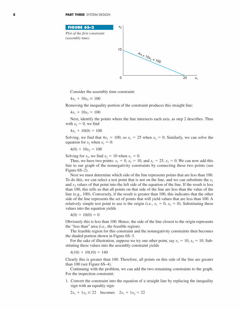
Consider the assembly time constraint:
4x1 � 10x2 � 100
Removing the inequality portion of the constraint produces this straight line:
4x1 � 10x2 � 100
Next, identify the points where the line intersects each axis, as step 2 describes. Thuswith x2 � 0, we find
4x1 � 10(0) � 100
Solving, we find that 4x1 � 100, so x1 � 25 when x2 � 0. Similarly, we can solve theequation for x2 when x1 � 0:
4(0) � 10x2 � 100
Solving for x2, we find x2 � 10 when x1 � 0.Thus, we have two points: x1 � 0, x2 � 10, and x1 � 25, x2 � 0. We can now add this
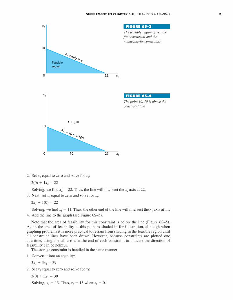
line to our graph of the nonnegativity constraints by connecting these two points (seeFigure 6S–2).
Next we must determine which side of the line represents points that are less than 100.To do this, we can select a test point that is not on the line, and we can substitute the x1
and x2 values of that point into the left side of the equation of the line. If the result is lessthan 100, this tells us that all points on that side of the line are less than the value of theline (e.g., 100). Conversely, if the result is greater than 100, this indicates that the otherside of the line represents the set of points that will yield values that are less than 100. Arelatively simple test point to use is the origin (i.e., x1 � 0, x2 � 0). Substituting thesevalues into the equation yields
4(0) � 10(0) � 0
Obviously this is less than 100. Hence, the side of the line closest to the origin representsthe “less than” area (i.e., the feasible region).
The feasible region for this constraint and the nonnegativity constraints then becomesthe shaded portion shown in Figure 6S–3.
For the sake of illustration, suppose we try one other point, say x1 � 10, x2 � 10. Sub-stituting these values into the assembly constraint yields
4(10) � 10(10) � 140
Clearly this is greater than 100. Therefore, all points on this side of the line are greaterthan 100 (see Figure 6S–4).
Continuing with the problem, we can add the two remaining constraints to the graph.For the inspection constraint:
1. Convert the constraint into the equation of a straight line by replacing the inequalitysign with an equality sign:
2x1 � 1x2 � 22 becomes 2x1 � 1x2 � 22
25 x10
10
x2
+ 10 = 100
x1
x2
4
FIGURE 6S–2
Plot of the first constraint(assembly time)
chapter6-suppliment.qxd 4/11/03 3:35 PM Page 8
SUPPLEMENT TO CHAPTER SIX LINEAR PROGRAMMING 9
2. Set x1 equal to zero and solve for x2:
2(0) � 1x2 � 22
Solving, we find x2 � 22. Thus, the line will intersect the x2 axis at 22.
3. Next, set x2 equal to zero and solve for x1:
2x1 � 1(0) � 22
Solving, we find x1 � 11. Thus, the other end of the line will intersect the x1 axis at 11.
4. Add the line to the graph (see Figure 6S–5).
Note that the area of feasibility for this constraint is below the line (Figure 6S–5).Again the area of feasibility at this point is shaded in for illustration, although whengraphing problems it is more practical to refrain from shading in the feasible region untilall constraint lines have been drawn. However, because constraints are plotted one at a time, using a small arrow at the end of each constraint to indicate the direction offeasibility can be helpful.
The storage constraint is handled in the same manner:
1. Convert it into an equality:
3x1 � 3x2 � 39
2. Set x1 equal to zero and solve for x2:
3(0) � 3x2 � 39
Solving, x2 � 13. Thus, x2 � 13 when x1 � 0.
25 x10
10
x2
Assembly timeFeasibleregion
FIGURE 6S–3
The feasible region, given thefirst constraint and thenonnegativity constraints
25 x10
10
10
x2
+ 10 = 100
x1
x2
4
• 10,10
FIGURE 6S–4
The point 10, 10 is above theconstraint line
chapter6-suppliment.qxd 4/11/03 3:35 PM Page 9

25 x10
10
22
11
x2
Inspection
Assembly
Feasible for inspectionbut not for assembly
Feasible forboth assemblyand inspection
Feasible for assemblybut not for inspection
FIGURE 6S–5
Partially completed graph,showing the assembly,inspection, and nonnegativityconstraints
25 x10
10
22
11 13
13
x2Inspection
Storage
Feasiblesolutionspace
Assembly
FIGURE 6S–6
Completed graph of themicrocomputer problemshowing all constraints and thefeasible solution space
3. Set x2 equal to zero and solve for x1:
3x1 � 3(0) � 39
Solving, x1 � 13. Thus, x1 � 13 when x2 � 0.
4. Add the line to the graph (see Figure 6S–6).
IDENTIFYING THE FEASIBLE SOLUTION SPACE
The feasible solution space is the set of all points that satisfies all constraints. (Recall thatthe x1 and x2 axes form nonnegativity constraints.) The shaded area shown in Figure 6S–6is the feasible solution space for our problem.
The next step is to determine which point in the feasible solution space will producethe optimal value of the objective function. This determination is made using the objectivefunction.
PLOTTING THE OBJECTIVE FUNCTION LINE
Plotting an objective function line involves the same logic as plotting a constraint line:Determine where the line intersects each axis. Recall that the objective function for themicrocomputer problem is
60x1 � 50x2
This is not an equation because it does not include an equal sign. We can get around thisby simply setting it equal to some quantity. Any quantity will do, although one that isevenly divisible by both coefficients is desirable.
10 PART THREE SYSTEM DESIGN
chapter6-suppliment.qxd 4/11/03 3:35 PM Page 10

SUPPLEMENT TO CHAPTER SIX LINEAR PROGRAMMING 11
Suppose we decide to set the objective function equal to 300. That is,
60x1 � 50x2 � 300
We can now plot the line of our graph. As before, we can determine the x1 and x2 inter-cepts of the line by setting one of the two variables equal to zero, solving for the other,and then reversing the process. Thus, with x1 � 0, we have
60(0) � 50x2 � 300
Solving, we find x2 � 6. Similarly, with x2 � 0, we have
60x1 � 50(0) � 300
Solving, we find x1 � 5. This line is plotted in Figure 6S–7.The profit line can be interpreted in the following way. It is an isoprofit line; every
point on the line (i.e., every combination of x1 and x2 that lies on the line) will provide a profit of $300. We can see from the graph many combinations that are both on the $300 profit line and within the feasible solution space. In fact, considering noninteger aswell as integer solutions, the possibilities are infinite.
Suppose we now consider another line, say the $600 line. To do this, we set the objec-tive function equal to this amount. Thus,
60x1 � 50x2 � 600
Solving for the x1 and x2 intercepts yields these two points:
x1 intercept x2 intercept
x1 � 10 x1 � 0
x2 � 0 x2 � 12
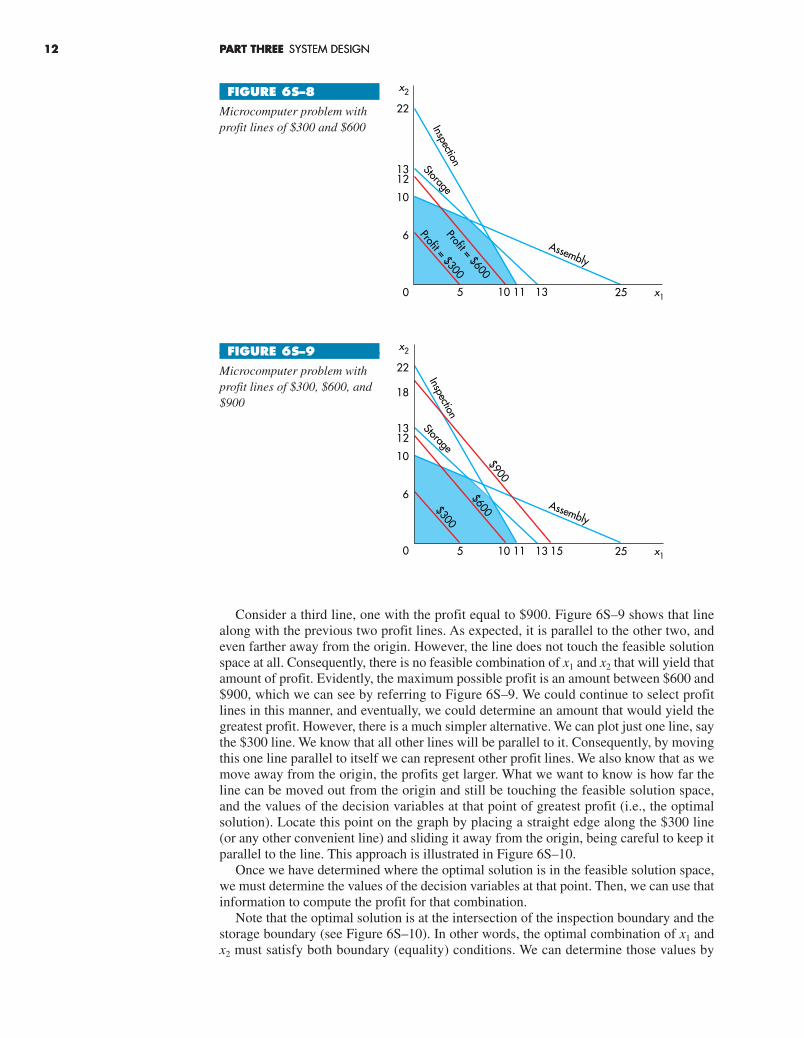
This line is plotted in Figure 6S–8, along with the previous $300 line for purposes ofcomparison.
Two things are evident in Figure 6S–8 regarding the profit lines. One is that the $600line is farther from the origin than the $300 line; the other is that the two lines are paral-lel. The lines are parallel because they both have the same slope. The slope is not affectedby the right side of the equation. Rather, it is determined solely by the coefficients 60 and50. It would be correct to conclude that regardless of the quantity we select for the valueof the objective function, the resulting line will be parallel to these two lines. Moreover,if the amount is greater than 600, the line will be even farther away from the origin thanthe $600 line. If the value is less than 300, the line will be closer to the origin than the$300 line. And if the value is between 300 and 600, the line will fall between the $300 and$600 lines. This knowledge will help in determining the optimal solution.
25 x10
10
22
115
6
13
13
x2
Inspection
Storage
Profit = $300
Assembly
FIGURE 6S–7
Microcomputer problem with$300 profit line added
chapter6-suppliment.qxd 4/11/03 3:35 PM Page 11
12 PART THREE SYSTEM DESIGN12 PART THREE SYSTEM DESIGN
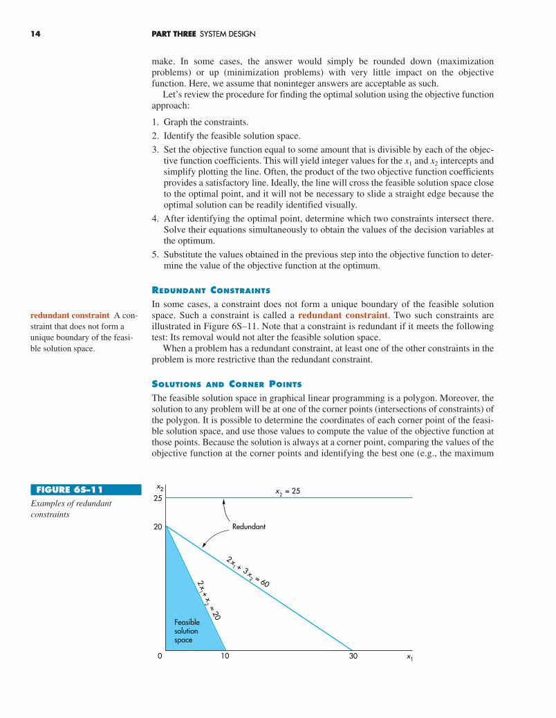
Consider a third line, one with the profit equal to $900. Figure 6S–9 shows that linealong with the previous two profit lines. As expected, it is parallel to the other two, andeven farther away from the origin. However, the line does not touch the feasible solutionspace at all. Consequently, there is no feasible combination of x1 and x2 that will yield thatamount of profit. Evidently, the maximum possible profit is an amount between $600 and$900, which we can see by referring to Figure 6S–9. We could continue to select profitlines in this manner, and eventually, we could determine an amount that would yield thegreatest profit. However, there is a much simpler alternative. We can plot just one line, saythe $300 line. We know that all other lines will be parallel to it. Consequently, by movingthis one line parallel to itself we can represent other profit lines. We also know that as wemove away from the origin, the profits get larger. What we want to know is how far theline can be moved out from the origin and still be touching the feasible solution space,and the values of the decision variables at that point of greatest profit (i.e., the optimalsolution). Locate this point on the graph by placing a straight edge along the $300 line (or any other convenient line) and sliding it away from the origin, being careful to keep itparallel to the line. This approach is illustrated in Figure 6S–10.
Once we have determined where the optimal solution is in the feasible solution space,we must determine the values of the decision variables at that point. Then, we can use thatinformation to compute the profit for that combination.
Note that the optimal solution is at the intersection of the inspection boundary and thestorage boundary (see Figure 6S–10). In other words, the optimal combination of x1 andx2 must satisfy both boundary (equality) conditions. We can determine those values by
25 x10
10
12
22
11105
6
13
13
x2
Inspection
Storage
Profit = $300Profit = $600
Assembly
FIGURE 6S–8
Microcomputer problem withprofit lines of $300 and $600
25 x10
10
12
22
18
11105
6
13 15
13
x2
Inspection
Storage
$300
$600$900
Assembly
FIGURE 6S–9
Microcomputer problem withprofit lines of $300, $600, and$900
chapter6-suppliment.qxd 4/11/03 3:35 PM Page 12

SUPPLEMENT TO CHAPTER SIX LINEAR PROGRAMMING 13
solving the two equations simultaneously. The equations are
Inspection 2x1 � 1x2 � 22
Storage 3x1 � 3x2 � 39
The idea behind solving two simultaneous equations is to algebraically eliminate one ofthe unknown variables (i.e., to obtain an equation with a single unknown). This can beaccomplished by multiplying the constants of one of the equations by a fixed amount andthen adding (or subtracting) the modified equation from the other. (Occasionally, it iseasier to multiply each equation by a fixed quantity.) For example, we can eliminate x2 bymultiplying the inspection equation by 3 and then subtracting the storage equation fromthe modified inspection equation. Thus,
3(2x1 � 1x2 � 22) becomes 6x1 � 3x2 � 66
Subtracting the storage equation from this produces
6x1 � 3x2 � 66
� (3x1 � 3x2 � 39)
3x1 � 0x2 � 27
Solving the resulting equation yields x1 � 9. The value of x2 can be found by substitutingx1 � 9 into either of the original equations or the modified inspection equation. Supposewe use the original inspection equation. We have
2(9) � 1x2 � 22
Solving, we find x2 � 4.Hence, the optimal solution to the microcomputer problem is to produce nine type 1
computers and four type 2 computers per day. We can substitute these values into theobjective function to find the optimal profit:
$60(9) � $50(4) � $740
Hence, the last line—the one that would last touch the feasible solution space as wemoved away from the origin parallel to the $300 profit line—would be the line whereprofit equalled $740.
In this problem, the optimal values for both decision variables are integers. This willnot always be the case; one or both of the decision variables may turn out to be non-integer. In some situations noninteger values would be of little consequence. This wouldbe true if the decision variables were measured on a continuous scale, such as the amountof water, sand, sugar, fuel oil, time, or distance needed for optimality, or if the contribu-tion per unit (profit, cost, etc.) were small, as with the number of nails or ball bearings to
25 x10
10
22
115
6
13
13
x2
Inspection
$300 AssemblyStorage
(last line)
Optimalsolution
FIGURE 6S–10
Finding the optimal solution tothe microcomputer problem
chapter6-suppliment.qxd 4/11/03 3:35 PM Page 13
14 PART THREE SYSTEM DESIGN14 PART THREE SYSTEM DESIGN
make. In some cases, the answer would simply be rounded down (maximizationproblems) or up (minimization problems) with very little impact on the objectivefunction. Here, we assume that noninteger answers are acceptable as such.
Let’s review the procedure for finding the optimal solution using the objective functionapproach:
1. Graph the constraints.
2. Identify the feasible solution space.
3. Set the objective function equal to some amount that is divisible by each of the objec-tive function coefficients. This will yield integer values for the x1 and x2 intercepts andsimplify plotting the line. Often, the product of the two objective function coefficientsprovides a satisfactory line. Ideally, the line will cross the feasible solution space closeto the optimal point, and it will not be necessary to slide a straight edge because theoptimal solution can be readily identified visually.
4. After identifying the optimal point, determine which two constraints intersect there.Solve their equations simultaneously to obtain the values of the decision variables atthe optimum.
5. Substitute the values obtained in the previous step into the objective function to deter-mine the value of the objective function at the optimum.
REDUNDANT CONSTRAINTS
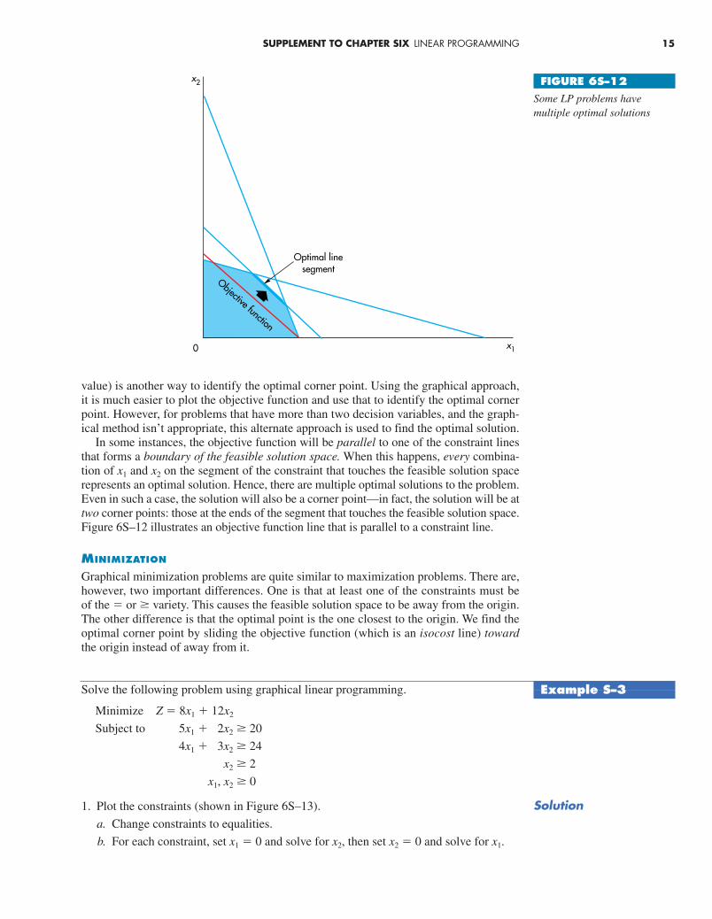
In some cases, a constraint does not form a unique boundary of the feasible solutionspace. Such a constraint is called a redundant constraint. Two such constraints areillustrated in Figure 6S–11. Note that a constraint is redundant if it meets the followingtest: Its removal would not alter the feasible solution space.
When a problem has a redundant constraint, at least one of the other constraints in theproblem is more restrictive than the redundant constraint.
SOLUTIONS AND CORNER POINTS
The feasible solution space in graphical linear programming is a polygon. Moreover, thesolution to any problem will be at one of the corner points (intersections of constraints) ofthe polygon. It is possible to determine the coordinates of each corner point of the feasi-ble solution space, and use those values to compute the value of the objective function atthose points. Because the solution is always at a corner point, comparing the values of theobjective function at the corner points and identifying the best one (e.g., the maximum
30 x10
20
25
10
x2
+ = 20
x1
x2
= 25x2
2
+ 3 = 60
x1
x2
2
Redundant
Feasiblesolutionspace
FIGURE 6S–11
Examples of redundantconstraints
redundant constraint A con-straint that does not form aunique boundary of the feasi-ble solution space.
chapter6-suppliment.qxd 4/11/03 3:35 PM Page 14
SUPPLEMENT TO CHAPTER SIX LINEAR PROGRAMMING 15
value) is another way to identify the optimal corner point. Using the graphical approach,it is much easier to plot the objective function and use that to identify the optimal cornerpoint. However, for problems that have more than two decision variables, and the graph-ical method isn’t appropriate, this alternate approach is used to find the optimal solution.
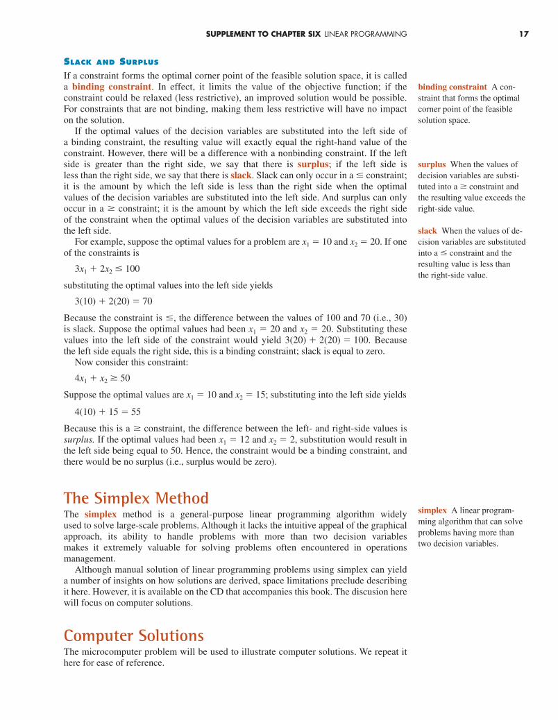
In some instances, the objective function will be parallel to one of the constraint linesthat forms a boundary of the feasible solution space. When this happens, every combina-tion of x1 and x2 on the segment of the constraint that touches the feasible solution spacerepresents an optimal solution. Hence, there are multiple optimal solutions to the problem.Even in such a case, the solution will also be a corner point—in fact, the solution will be attwo corner points: those at the ends of the segment that touches the feasible solution space.Figure 6S–12 illustrates an objective function line that is parallel to a constraint line.
MINIMIZATION
Graphical minimization problems are quite similar to maximization problems. There are,however, two important differences. One is that at least one of the constraints must be of the � or � variety. This causes the feasible solution space to be away from the origin.The other difference is that the optimal point is the one closest to the origin. We find theoptimal corner point by sliding the objective function (which is an isocost line) towardthe origin instead of away from it.
Solve the following problem using graphical linear programming.
Minimize Z � 8x1 � 12x2
Subject to 5x1 � 2x2 � 20
4x1 � 3x2 � 24
x2 � 2
x1, x2 � 0
1. Plot the constraints (shown in Figure 6S–13).
a. Change constraints to equalities.
b. For each constraint, set x1 � 0 and solve for x2, then set x2 � 0 and solve for x1.
x10
x2
Objective function
Optimal linesegment
FIGURE 6S–12
Some LP problems havemultiple optimal solutions
Example S–3
Solution
chapter6-suppliment.qxd 4/11/03 3:35 PM Page 15

16 PART THREE SYSTEM DESIGN16 PART THREE SYSTEM DESIGN
c. Graph each constraint. Note that x2 � 2 is a horizontal line parallel to the x1 axisand 2 units above it.
2. Shade the feasible solution space (see Figure 6S–13).
3. Plot the objective function.
a. Select a value for the objective function that causes it to cross the feasible solutionspace. Try 8 � 12 � 96; 8x1 � 12x2 � 96 (acceptable).
b. Graph the line (see Figure 6S–14).
4. Slide the objective function toward the origin, being careful to keep it parallel to theoriginal line.
5. The optimum (last feasible point) is shown in Figure 6S–14. The x2 coordinate (x2 �2) can be determined by inspection of the graph. Note that the optimum point is at theintersection of the line x2 � 2 and the line 4x1 � 3x2 � 24. Substituting the value of x2
� 2 into the latter equation will yield the value of x1 at the intersection:
4x1 � 3(2) � 24 x1 � 4.5
Thus, the optimum is x1 � 4.5 units and x2 � 2.
6. Compute the minimum cost:
8x1 � 12x2 � 8(4.5) � 12(2) � 60
2 4 6 8 10 12 x10
2
4
6
8
x2
14
10
12
Feasiblesolutionspace
5 + 2 = 20 x 2
x 1
4 + 3 = 24
x2
= 2x2
x1
FIGURE 6S–13
The constraints define thefeasible solution space
2 4 6 8 10 12 x10
2
4
6
8
x2
14
10
12
8 + 12 = $96
x2
x1
Optimum
Objectivefunction
FIGURE 6S–14
The optimum is the last pointthe objective function touchesas it is moved toward theorigin
chapter6-suppliment.qxd 4/11/03 3:35 PM Page 16
SLACK AND SURPLUS
If a constraint forms the optimal corner point of the feasible solution space, it is called a binding constraint. In effect, it limits the value of the objective function; if theconstraint could be relaxed (less restrictive), an improved solution would be possible.For constraints that are not binding, making them less restrictive will have no impact on the solution.
If the optimal values of the decision variables are substituted into the left side of a binding constraint, the resulting value will exactly equal the right-hand value of theconstraint. However, there will be a difference with a nonbinding constraint. If the leftside is greater than the right side, we say that there is surplus; if the left side is less than the right side, we say that there is slack. Slack can only occur in a � constraint;it is the amount by which the left side is less than the right side when the optimal values of the decision variables are substituted into the left side. And surplus can onlyoccur in a � constraint; it is the amount by which the left side exceeds the right side of the constraint when the optimal values of the decision variables are substituted into the left side.
For example, suppose the optimal values for a problem are x1 � 10 and x2 � 20. If oneof the constraints is
3x1 � 2x2 � 100
substituting the optimal values into the left side yields
3(10) � 2(20) � 70
Because the constraint is �, the difference between the values of 100 and 70 (i.e., 30) is slack. Suppose the optimal values had been x1 � 20 and x2 � 20. Substituting thesevalues into the left side of the constraint would yield 3(20) � 2(20) � 100. Because the left side equals the right side, this is a binding constraint; slack is equal to zero.
Now consider this constraint:
4x1 � x2 � 50
Suppose the optimal values are x1 � 10 and x2 � 15; substituting into the left side yields
4(10) � 15 � 55
Because this is a � constraint, the difference between the left- and right-side values issurplus. If the optimal values had been x1 � 12 and x2 � 2, substitution would result inthe left side being equal to 50. Hence, the constraint would be a binding constraint, andthere would be no surplus (i.e., surplus would be zero).
The Simplex MethodThe simplex method is a general-purpose linear programming algorithm widely used to solve large-scale problems. Although it lacks the intuitive appeal of the graphicalapproach, its ability to handle problems with more than two decision variables makes it extremely valuable for solving problems often encountered in operationsmanagement.
Although manual solution of linear programming problems using simplex can yield a number of insights on how solutions are derived, space limitations preclude describingit here. However, it is available on the CD that accompanies this book. The discusion herewill focus on computer solutions.
Computer SolutionsThe microcomputer problem will be used to illustrate computer solutions. We repeat ithere for ease of reference.
SUPPLEMENT TO CHAPTER SIX LINEAR PROGRAMMING 17
binding constraint A con-straint that forms the optimalcorner point of the feasiblesolution space.
surplus When the values ofdecision variables are substi-tuted into a � constraint andthe resulting value exceeds theright-side value.
slack When the values of de-cision variables are substitutedinto a � constraint and theresulting value is less than the right-side value.
simplex A linear program-ming algorithm that can solveproblems having more thantwo decision variables.
chapter6-suppliment.qxd 4/11/03 3:35 PM Page 17

18 PART THREE SYSTEM DESIGN18 PART THREE SYSTEM DESIGN
Maximize 60x1 � 50x2 where x1 � the number of type 1 computers
x2 � the number of type 2 computers
Subject to
Assembly 4x1 � 10x2 � 100 hours
Inspection 2x1 � 1x2 � 22 hours
Storage 3x1 � 3x2 � 39 cubic feet
x1, x2 � 0
SOLVING LP MODELS USING MS EXCEL
Solutions to linear programming models can be obtained from spreadsheet softwaresuch as Microsoft’s Excel. Excel has a routine called Solver that performs the necessarycalculations.
To use Solver:1. First, enter the problem in a worksheet, as shown in Figure 6S–15. What is not
obvious from the figure is the need to enter a formula for each cell where there is a zero(Solver automatically inserts the zero after you input the formula). The formulas are forthe value of the objective function and the constraints, in the appropriate cells. Before youenter the formulas, designate the cells where you want the optimal values of x1 and x2.Here, cells D4 and E4 are used. To enter a formula, click on the cell that the formula willpertain to, and then enter the formula, starting with an equals sign. We want the optimalvalue of the objective function to appear in cell G4. For G4, enter the formula
� 60*D4 � 50*E4
The constraint formulas, in cells C7, C8, and C9, are
for C7: � 4*D4 � 10*E4for C8: � 2*D4 � 1*E4for C9: � 3*D4 � 3*E4
FIGURE 6S–15
MS Excel worksheet formicrocomputer problem
chapter6-suppliment.qxd 4/11/03 3:35 PM Page 18

SUPPLEMENT TO CHAPTER SIX LINEAR PROGRAMMING 19
2. Now, click on Tools on the top of the worksheet, and in that menu, click on Solver.The Solver menu will appear as illustrated in Figure 6S–16. Begin by setting the TargetCell (i.e., indicating the cell where you want the optimal value of the objective functionto appear). Note, if the activated cell is the cell designated for the value of Z when youclick on the Tools menu, Solver will automatically set that cell as the target cell.
Highlight Max if it isn’t already highlighted. The Changing Cells are the cells whereyou want the optimal values of the decision variables to appear. Here, they are cells D4and E4. We indicate this by the range D4:E4 (Solver will add the $ signs).
Finally, add the constraints by clicking on Add … When that menu appears, for eachconstraint, enter the cell that contains the formula for the left side of the constraint, then se-lect the appropriate inequality sign, and then enter either the right-side amount or the cellthat has the right-side amount. Here, the right-side amounts are used. After you have en-tered each constraint, click on Add, and then enter the next constraint. (Note, constraintscan be entered in any order.) For the nonnegativity constraints, enter the range of cells des-ignated for the optimal values of the decision variables, choose � sign, and enter 0 for theright-hand side. Then, click on OK rather than Add, and you will return to the Solvermenu. Click on Options … , and in the Options menu, click on Assume Linear Model, andthen click on OK. This will return you to the Solver Parameters menu. Click on Solve.
3. The Solver Results menu will then appear, indicating that a solution has been found,or that an error has occurred. If there has been an error, go back to the Solver Parametersmenu and check to see that your constraints refer to the correct changing cells, and thatthe inequality directions are correct. Make the corrections and click on Solve.
Assuming everything is correct, in the Solver Results menu, in the Reports box, high-light both Answer and Sensitivity, and then click on OK.
4. Solver will incorporate the optimal values of the decision variables and the objectivefunction in your original layout on your worksheet (see Figure 6S–17). We can see that the optimal values are type 1 � 9 units and type 2 � 4 units, and the total profit is 740. Theanswer report will also show the optimal values of the decision variables (upper part ofFigure 6S–18), and some information on the constraints (lower part of Figure 6S–18). Ofparticular interest here is the indication of which constraints have slack and how muchslack. We can see that the constraint entered in cell C7 (assembly) has a slack of 24, and
FIGURE 6S–16
MS Excel Solver parametersfor microcomputer problem
chapter6-suppliment.qxd 4/11/03 3:35 PM Page 19
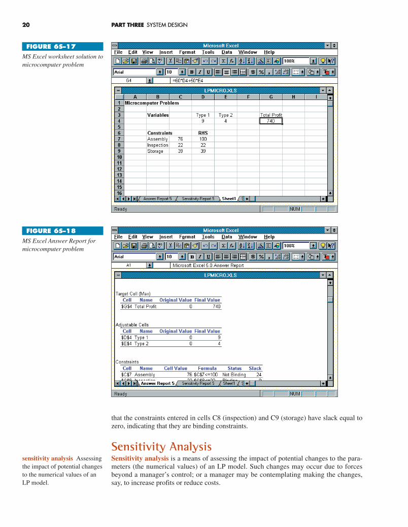
20 PART THREE SYSTEM DESIGN
that the constraints entered in cells C8 (inspection) and C9 (storage) have slack equal tozero, indicating that they are binding constraints.
Sensitivity AnalysisSensitivity analysis is a means of assessing the impact of potential changes to the para-meters (the numerical values) of an LP model. Such changes may occur due to forcesbeyond a manager’s control; or a manager may be contemplating making the changes,say, to increase profits or reduce costs.
20 PART THREE SYSTEM DESIGN
FIGURE 6S–17
MS Excel worksheet solution tomicrocomputer problem
FIGURE 6S–18
MS Excel Answer Report formicrocomputer problem
sensitivity analysis Assessingthe impact of potential changesto the numerical values of anLP model.
chapter6-suppliment.qxd 4/11/03 3:35 PM Page 20
SUPPLEMENT TO CHAPTER SIX LINEAR PROGRAMMING 21
There are three types of potential changes:
1. Objective function coefficients.
2. Right-hand values of constraints.
3. Constraint coefficients.
We will consider the first two of these here. We begin with changes to objective functioncoefficients.
OBJECTIVE FUNCTION COEFFICIENT CHANGES
A change in the value of an objective function coefficient can cause a change in the opti-mal solution of a problem. In a graphical solution, this would mean a change to anothercorner point of the feasible solution space. However, not every change in the value of anobjective function coefficient will lead to a changed solution; generally there is a range ofvalues for which the optimal values of the decision variables will not change. For exam-ple, in the microcomputer problem, if the profit on type 1 computers increased from $60per unit to, say, $65 per unit, the optimal solution would still be to produce nine units oftype 1 and four units of type 2 computers. Similarly, if the profit per unit on type 1 com-puters decreased from $60 to, say, $58, producing nine of type 1 and four of type 2 wouldstill be optimal. These sorts of changes are not uncommon; they may be the result of suchthings as price changes in raw materials, price discounts, cost reductions in production,and so on. Obviously, when a change does occur in the value of an objective function co-efficient, it can be helpful for a manager to know if that change will affect the optimalvalues of the decision variables. The manager can quickly determine this by referring tothat coefficient’s range of optimality, which is the range in possible values of that objec-tive function coefficient over which the optimal values of the decision variables will notchange. Before we see how to determine the range, consider the implication of the range.The range of optimality for the type 1 coefficient in the microcomputer problem is 50 to100. That means that as long as the coefficient’s value is in that range, the optimal valueswill be 9 units of type 1 and 4 units of type 2. Conversely, if a change extends beyond the range of optimality, the solution will change.
Similarly suppose instead the coefficient of type 2 computers were to change. Its rangeof optimality is 30 to 60. As long as the value of the change doesn’t take it outside of thisrange, nine and four will still be the optimal values. Note, however, even for changes thatare within the range of optimality, the optimal value of the objective function will change.If the type 1 coefficient increased from $60 to $61, and nine units of type 1 is still opti-mum, profit would increase by $9: nine units times $1 per unit. Thus, for a change that iswithin the range of optimality, a revised value of the objective function must be deter-mined.
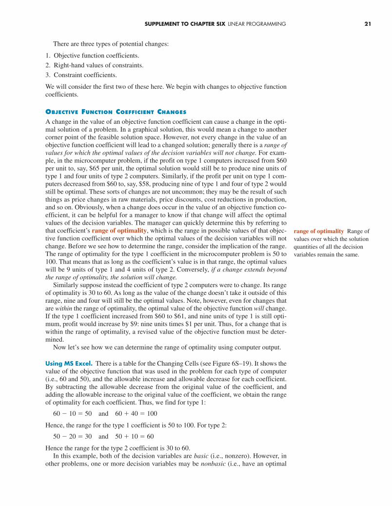
Now let’s see how we can determine the range of optimality using computer output.
Using MS Excel. There is a table for the Changing Cells (see Figure 6S–19). It shows thevalue of the objective function that was used in the problem for each type of computer(i.e., 60 and 50), and the allowable increase and allowable decrease for each coefficient.By subtracting the allowable decrease from the original value of the coefficient, andadding the allowable increase to the original value of the coefficient, we obtain the rangeof optimality for each coefficient. Thus, we find for type 1:
60 � 10 � 50 and 60 � 40 � 100
Hence, the range for the type 1 coefficient is 50 to 100. For type 2:
50 � 20 � 30 and 50 � 10 � 60
Hence the range for the type 2 coefficient is 30 to 60.In this example, both of the decision variables are basic (i.e., nonzero). However, in
other problems, one or more decision variables may be nonbasic (i.e., have an optimal
range of optimality Range ofvalues over which the solutionquantities of all the decisionvariables remain the same.
chapter6-suppliment.qxd 4/11/03 3:35 PM Page 21

22 PART THREE SYSTEM DESIGN
value of zero). In such instances, unless the value of that variable’s objective functioncoefficient increases by more than a certain amount called its reduced cost, it won’t comeinto solution (i.e., become a basic variable). Hence, the range of optimality (sometimesreferred to as the range of insignificance) for a nonbasic variable is from negative infinityto the sum of its current value and its reduced cost.
Now let’s see how we can handle multiple changes to objective function coefficients;that is, a change in more than one coefficient. To do this, divide each coefficient’s changeby the allowable change in the same direction. Thus, if the change is a decrease, dividethat amount by the allowable decrease. Treat all resulting fractions as positive. Sum the fractions. If the sum does not exceed 1.00, then multiple changes are within the rangeof optimality and will not result in any change to the optimal values of the decisionvariables.
CHANGES IN THE RIGHT-HAND-SIDE (RHS) VALUE OF A CONSTRAINT
In considering right-hand-side changes, it is important to know if a particular constraint is binding on a solution. A constraint is binding if substituting the values of the decisionvariables of that solution into the left side of the constraint results in a value that is equal to the RHS value. In other words, that constraint stops the objective function fromachieving a better value (e.g., a greater profit or a lower cost). Each constraint has a corresponding shadow price, which is a marginal value that indicates the amount by which the value of the objective function would change if there were a one-unit changein the RHS value of that constraint. If a constraint is nonbinding, its shadow price is zero, meaning that increasing or decreasing its RHS value by one unit will have no impact on the value of the objective function. Nonbinding constraints have either slack (if the constraint is �) or surplus (if the constraint is �). Suppose a constraint has 10 unitsof slack in the optimal solution, which means 10 units that are unused. If we were toincrease or decrease the constraint’s RHS value by one unit, the only effect would be to increase or decrease its slack by one unit. But there is no profit associated with slack,so the value of the objective function wouldn’t change. On the other hand, if the changeis to the RHS value of a binding constraint, then the optimal value of the objective
22 PART THREE SYSTEM DESIGN
FIGURE 6S–19
MS Excel sensitivity report formicrocomputer problem
shadow price Amount bywhich the value of the objec-tive function would changewith a one-unit change in theRHS value of a constraint.
chapter6-suppliment.qxd 4/11/03 3:35 PM Page 22

function would change. Any change in a binding constraint will cause the optimal valuesof the decision variables to change, and hence cause the value of the objective function tochange. For example, in the microcomputer problem, the inspection constraint is a binding constraint; it has a shadow price of 10. That means if there was one hour less of inspection time, total profit would decrease by $10, or if there were one more hour ofinspection time available, total profit would increase by $10. In general, multiplying theamount of change in the RHS value of a constraint by the constraint’s shadow price willindicate the change’s impact on the optimal value of the objective function. However, thisis true only over a limited range called the range of feasibility. In this range, the value ofthe shadow price remains constant. Hence, as long as a change in the RHS value of a con-straint is within its range of feasibility, the shadow price will remain the same, and onecan readily determine the impact on the objective function.
Let’s see how to determine the range of feasibility from computer output.
Using MS Excel. In the sensitivity report there is a table labelled “Constraints” (seeFigure 6S–19). The table shows the shadow price for each constraint, its RHS value, andthe allowable increase and allowable decrease. Adding the allowable increase to the RHSvalue and subtracting the allowable decrease will produce the range of feasibility for thatconstraint. For example, for the inspection constraint the range would be
22 � 4 � 26; 22 � 4 � 18
Hence, the range of feasibility for Inspection is 18 to 26 hours. Similarly, for the storageconstraint, the range is
39 � 6 � 33 to 39 � 4.5 � 43.5
The range for the assembly constraint is a little different; the assembly constraint isnonbinding (note the shadow price of 0) while the other two are binding (note theirnonzero shadow prices). The assembly constraint has a slack of 24 (the differencebetween its RHS value of 100 and its final value of 76). With its slack of 24, its RHS value could be decreased by as much as 24 (to 76) before it would become binding.Conversely, increasing its right-hand side will only produce more slack. Thus, no amountof increase in the RHS value will make it binding, so there is no upper limit on the allow-able increase. Excel indicates this by the large value (1E�30) shown for the allowable in-crease. So its range of feasibility has a lower limit of 76 and no upper limit.
If there are changes to more than one constraint’s RHS value, analyze these in the sameway as multiple changes to objective function coefficients. That is, if the change is anincrease, divide that amount by that constraint’s allowable increase; if the change is adecrease, divide the decrease by the allowable decrease. Treat all resulting fractions aspositives. Sum the fractions. As long as the sum does not exceed 1.00, the changes arewithin the range of feasibility for multiple changes, and the shadow prices won’t change.
Table 6S–1 summarizes the impacts of changes that fall within either the range ofoptimality or the range of feasibility.
Now let’s consider what happens if a change goes beyond a particular range. In asituation involving the range of optimality, a change in an objective function that is beyondthe range of optimality will result in a new solution. Hence, it will be necessary torecompute the solution. For a situation involving the range of feasibility, there are twocases to consider. The first case would be increasing the RHS value of a � constraint to beyond the upper limit of its range of feasibility. This would produce slack equal to the amount by which the upper limit is exceeded. Hence, if the upper limit is 200,and the increase is 220, the result is that the constraint has a slack of 20. Similarly, for a � constraint, going below its lower bound creates a surplus for that constraint. The secondcase for each of these would be exceeding the opposite limit (the lower bound for a � constraint, or the upper bound for a � constraint). In either instance, a new solutionwould have to be generated.
SUPPLEMENT TO CHAPTER SIX LINEAR PROGRAMMING 23
range of feasibility Range ofvalues for the RHS of a con-straint over which the shadowprice remains the same.
chapter6-suppliment.qxd 4/11/03 3:35 PM Page 23

24 PART THREE SYSTEM DESIGN24 PART THREE SYSTEM DESIGN
CHANGES TO OBJECTIVE FUNCTIONCOEFFICIENTS THAT ARE WITHIN THERANGE OF OPTIMALITY
Component Result
Values of decision variables No changeValue of objective function Will change
CHANGES TO RHS VALUES OFCONSTRAINTS THAT ARE WITHIN THE RANGE OF FEASIBILITY
Component Result
Value of shadow price No changeList of basic variables No changeValues of basic variables Will changeValue of objective function Will change
TABLE 6S–1
Summary of the impact ofchanges within their respectiveranges
Solved Problems
Problem 1
Key Terms binding constraint, 17constraints, 3decision variables, 2feasible solution space, 3graphical linear programming, 5objective function, 2parameters, 3range of feasibility, 23
range of optimality, 21redundant constraint, 14sensitivity analysis, 20shadow price, 22simplex, 17slack, 17surplus, 17
1For the sake of consistency, we will assign to the horizontal axis the first decision variable mentioned in the problem. In this case, variable A will be represented on the horizontal axis and variable B on thevertical axis.
Solution
A small construction firm specializes in building and selling single-family homes. The firm offers two basic types of houses, model A and model B. Model A houses require 4,000labour hours, 2 tons of stone, and 2,000 board feet of lumber. Model B houses require 10,000 labour hours, 3 tons of stone, and 2,000 board feet of lumber. Due to long lead times forordering supplies and the scarcity of skilled and semiskilled workers in the area, the firm will beforced to rely on its present resources for the upcoming building season. It has 400,000 hours of labour, 150 tons of stone, and 200,000 board feet of lumber. What mix of model A and Bhouses should the firm construct if model As yield a profit of $1,000 per unit and model Bs yield$2,000 per unit? Assume that the firm will be able to sell all the units it builds.
a. Formulate the objective function and constraints:1
Maximize Z � 1,000A � 2,000BSubject to
Labour 4,000A � 10,000B � 400,000 labour hoursStone 2A � 3B � 150 tonsLumber 2,000A � 2,000B � 200,000 board feet
A, B � 0
b. Graph the constraints and objective function, and identify the optimum corner point (seegraph). Note that the lumber constraint is redundant: It does not form a boundary of thefeasible solution space.
chapter6-suppliment.qxd 4/11/03 3:35 PM Page 24
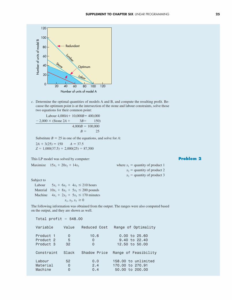
SUPPLEMENT TO CHAPTER SIX LINEAR PROGRAMMING 25
c. Determine the optimal quantities of models A and B, and compute the resulting profit. Be-cause the optimum point is at the intersection of the stone and labour constraints, solve thosetwo equations for their common point:
Labour 4,000A� 10,000B� 400,000� 2,000 � (Stone 2A � 3B� 150)
4,000B � 100,000B � 25
Substitute B � 25 in one of the equations, and solve for A:
2A � 3(25) � 150 A � 37.5Z � 1,000(37.5) � 2,000(25) � 87,500
This LP model was solved by computer:
Maximize 15x1 � 20x2 � 14x3 where x1 � quantity of product 1x2 � quantity of product 2x3 � quantity of product 3
Subject toLabour 5x1 � 6x2 � 4x3 � 210 hoursMaterial 10x1 � 8x2 � 5x3 � 200 poundsMachine 4x1 � 2x2 � 5x3 � 170 minutes
x1, x2, x3 � 0
The following information was obtained from the output. The ranges were also computed basedon the output, and they are shown as well.
Total profit � 548.00
Variable Value Reduced Cost Range of Optimality
Product 1 0 10.6 0.00 to 25.60Product 2 5 0 9.40 to 22.40Product 3 32 0 12.50 to 50.00
Constraint Slack Shadow Price Range of Feasibility
Labour 52 0.0 158.00 to unlimitedMaterial 0 2.4 170.00 to 270.91Machine 0 0.4 50.00 to 200.00
20 40 60 80 100 1200
20
40
60
80
100
120
Number of units of model A
Num
ber
of u
nits
of m
odel
B
Redundant
Lumber
Optimum
Labor
Stone
Problem 2
chapter6-suppliment.qxd 4/11/03 3:35 PM Page 25

26 PART THREE SYSTEM DESIGN26 PART THREE SYSTEM DESIGN
a. Which decision variables are basic (i.e., in solution)?b. By how much would the profit per unit of product 1 have to increase in order for it to have a
nonzero value (i.e., for it to become a basic variable)?c. If the profit per unit of product 2 increased by $2 to $22, would the optimal production quan-
tities of products 2 and 3 change? Would the optimal value of the objective function change?d. If the available amount of labour decreased by 12 hours, would that cause a change in the
optimal values of the decision variables or the optimal value of the objective function? Wouldanything change?
e. If the available amount of material increased by 10 pounds to 210 pounds, how would thataffect the optimal value of the objective function?
f. If profit per unit on product 2 increased by $1 and profit per unit on product 3 decreased by$.50, would that fall within the range of multiple changes? Would the values of the decisionvariables change? What would be the revised value of the objective function?
a. Products 2 and 3 are in solution (i.e., have nonzero values; the optimal value of product 2 is5 units, and the optimal value of product 3 is 32 units).
b. The amount of increase would have to equal its reduced cost of $10.60.c. No, because the change would be within its range of optimality, which has an upper limit of
$22.40. The objective function value would increase by an amount equal to the quantity of product 2 and its increased unit profit. Hence, it would increase by 5($2) � $10 to $558.
d. Labour has a slack of 52 hours. Consequently, the only effect would be to decrease the slackto 40 hours.
e. The change is within the range of feasibility. The objective function value will increase bythe amount of change multiplied by material’s shadow price of $2.40. Hence, the objectivefunction value would increase by 10($2.40) � $24.00. (Note: If the change had been adecrease of 10 pounds, which is also within the range of feasibility, the value of the objec-tive function would have decreased by this amount.)
f. To determine if the changes are within the range for multiple changes, we first compute theratio of the amount of each change to the end of the range in the same direction. For product2, it is $1/$2.40 � .417; for product 3, it is � $.50/� $1.50 � .333. Next, we compute thesum of these ratios: .417 �.333 � .750. Because this does not exceed 1.00, we conclude thatthese changes are within the range. This means that the optimal values of the decision vari-ables will not change. We can compute the change to the value of the objective function by multiplying each product’s optimal quantity by its changed profit per unit: 5($1) �32(� $.50) � � $11. Hence, with these changes, the value of the objective function woulddecrease by $11; its new value would be $548 � $11 � $537.
Solution
1. For which decision environment is linear programming most suited?2. What is meant by the term feasible solution space? What determines this region?3. Explain the term redundant constraint.4. What is an isocost line? An isoprofit line?5. What does sliding an objective function line toward the origin represent? Away from the origin?6. Briefly explain these terms:
a. Basic variableb. Shadow pricec. Range of feasibilityd. Range of optimalitye. Redundant constraints
Discussion and Review Questions
1. Solve these problems using graphical linear programming and answer the questions that fol-low. Use simultaneous equations to determine the optimal values of the decision variables.a. Maximize Z � 4x1 � 3x2
Problems
chapter6-suppliment.qxd 4/11/03 3:35 PM Page 26

Subject toMaterial 6x1 � 4x2 � 48 kgLabour 4x1 � 8x2 � 80 hr
x1, x2 � 0b. Maximize Z � 2x1 �10x2
Subject toR 10x1 � 4x2 � 40S 1x1 � 6x2 � 24T 1x1 � 2x2 � 14
x1, x2 � 0c. Maximize Z � 6A � 3B (revenue)
Subject toMaterial 20A � 6B � 600 kgMachinery 25A � 20B� 1,000 hrLabour 20A � 30B� 1,200 hr
A, B � 0
(1) What are the optimal values of the decision variables and Z?(2) Do any constraints have (nonzero) slack? If yes, which one(s) and how much slack does
each have?(3) Do any constraints have (nonzero) surplus? If yes, which one(s) and how much surplus
does each have?(4) Are any constraints redundant? If yes, which one(s)? Explain briefly.
2. Solve these problems using graphical linear programming and then answer the questions thatfollow. Use simultaneous equations to determine the optimal values of the decision variables.a. Minimize Z � 1.80S � 2.20T
Subject toPotassium 5S � 8T � 200 gramsCarbohydrate 15S � 6T � 240 gramsProtein 4S � 12T � 180 gramsT T � 10 grams
S, T � 0b. Minimize Z � 2x1 � 3x2
Subject toD 4x1 � 2x2 � 20E 2x1 � 6x2 � 18F 1x1 � 2x2 � 12
x1, x2 � 0
(1) What are the optimal values of the decision variables and Z?(2) Do any constraints have (nonzero) slack? If yes, which one(s) and how much slack does
each have?(3) Do any constraints have (nonzero) surplus? If yes, which one(s) and how much surplus
does each have?(4) Are any constraints redundant? If yes, which one(s)? Explain briefly.
3. An appliance manufacturer produces two models of microwave ovens: H and W. Both modelsrequire fabrication and assembly work; each H uses four hours of fabrication and two hours ofassembly, and each W uses two hours of fabrication and six hours of assembly. There are 600fabrication hours available this week and 480 hours of assembly. Each H contributes $40 toprofits, and each W contributes $30 to profits. What quantities of H and W will maximizeprofits?
4. A small candy shop is preparing for the holiday season. The owner must decide how manybags of deluxe mix and how many bags of standard mix of Peanut/Raisin Delite to put up. Thedeluxe mix has 2/3 kg raisins and 1/3 kg peanuts, and the standard mix has 1/2 kg raisins and 1/2 kg peanuts per bag. The shop has 90 kg of raisins and 60 kg of peanuts to work with.
SUPPLEMENT TO CHAPTER SIX LINEAR PROGRAMMING 27
chapter6-suppliment.qxd 4/11/03 3:35 PM Page 27
28 PART THREE SYSTEM DESIGN28 PART THREE SYSTEM DESIGN
Peanuts cost $.60 per kg and raisins cost $1.50 per kg. The deluxe mix will sell for $2.90per kg, and the standard mix will sell for $2.55 per kg. The owner estimates that no more than110 bags of one type can be sold.a. If the goal is to maximize profits, how many bags of each type should be prepared?b. What is the expected profit?
5. A retired couple supplement their income by making fruit pies, which they sell to a local gro-cery store. During the month of September, they produce apple and grape pies. The apple piesare sold for $1.50 to the grocer, and the grape pies are sold for $1.20. The couple is able to sellall of the pies they produce owing to their high quality. They use fresh ingredients. Flour andsugar are purchased once each month. For the month of September, they have 1,200 cups of sugar and 2,100 cups of flour. Each apple pie requires 11/2 cups of sugar and 3 cups of flour,and each grape pie requires 2 cups of sugar and 3 cups of flour.a. Determine the number of grape and the number of apple pies that will maximize revenues
if the couple working together can make an apple pie in six minutes and a grape pie in threeminutes. They plan to work no more than 60 hours.
b. Determine the amounts of sugar, flour, and time that will be unused.6. Solve each of these problems by computer and obtain the optimal values of the decision
variables and the objective function.a. Maximize 4x1 � 2x2 � 5x3
Subject to1x1 � 2x2 � 1x3 � 251x1 � 4x2 � 2x3 � 403x1 � 3x2 � 1x3 � 30
x1, x2, x3 � 0b. Maximize 10x1 � 6x2 � 3x3
Subject to1x1 � 1x2 � 2x3 � 252x1 � 1x2 � 4x3 � 401x1 � 2x2 � 3x3 � 40
x1, x2, x3 � 07. For Problem 6a, determine the following:
a. The range of feasibility for each constraint.b. The range of optimality for the coefficients of the objective function.
8. For Problem 6b:a. Find the range of feasibility for each constraint, and interpret your answers.b. Determine the range of optimality for each coefficient of the objective function. Interpret
your results.9. A small firm makes three similar products, which all follow the same three-step process, con-
sisting of milling, inspection, and drilling. Product A requires 12 minutes of milling, 5 minutesfor inspection, and 10 minutes of drilling per unit; product B requires 10 minutes of milling,4 minutes for inspection, and 8 minutes of drilling per unit; and product C requires 8 minutes of milling, 4 minutes for inspection, and 16 minutes of drilling. The department has 20 hoursavailable during the next period for milling, 15 hours for inspection, and 24 hours for drilling.Product A contributes $2.40 per unit to profit, B contributes $2.50 per unit, and C contributes$3.00 per unit. Determine the optimal mix of products in terms of maximizing contribution toprofits for the period. Then, find the range of optimality for the profit coefficient of each variable.
10. Formulate and then solve a linear programming model of this problem, to determine how manycontainers of each product to produce tomorrow to maximize profits. The company makes fourjuice products using orange, grapefruit, and pineapple juice.
Product Retail Price/Litre
Orange juice $1.00Grapefruit juice .90Pineapple juice .80All-in-One 1.10
chapter6-suppliment.qxd 4/11/03 3:35 PM Page 28
The All-in-One juice has equal parts of orange, grapefruit, and pineapple juice. Each productis produced in a one-litre size. On hand are 1,600 litres of orange juice, 1,200 litres of grape-fruit juice, and 800 litres of pineapple juice. The cost per litre is $0.50 for orange juice, $0.40for grapefruit juice, and $0.35 for pineapple juice.
In addition, the manager wants grapefruit juice to be used for no more than 30 percent ofthe number of containers produced. She wants the ratio of the number of containers of orangejuice to the number of containers of pineapple juice to be at least 7 to 5.
11. A wood products firm uses leftover time at the end of each week to make goods for stock. Cur-rently, two products on the list of items are produced for stock: a chopping board and a knifeholder. Both items require three operations: cutting, gluing, and finishing. The manager of thefirm has collected the following data on these products:
TIME PER UNIT (MINUTES)
Item Profit/Unit Cutting Gluing Finishing
Chopping board $2 1.4 5 12Knife holder $6 0.8 13 3
The manager has also determined that, during each week, 56 minutes are available for cutting,650 minutes are available for gluing, and 360 minutes are available for finishing.a. Determine the optimal quantities of the decision variables.b. Which resources are not completely used by your solution? How much of each resource is
unused?12. The manager of the deli section of a grocery superstore has just learned that the department has
112 kg of mayonnaise, of which 70 kg is approaching its expiration date and must be used. Touse up the mayonnaise, the manager has decided to prepare two items: a ham spread and a delispread. Each pan of the ham spread will require 1.4 kg of mayonnaise, and each pan of the deli spread will require 1.0 kg. The manager has received an order for 10 pans of ham spreadand 8 pans of the deli spread. In addition, the manager has decided to have at least 10 pans ofeach spread available for sale. Both spreads will cost $3 per pan to make, but ham spread sellsfor $5 per pan and deli spread sells for $7 per pan.a. Determine the solution that will minimize cost.b. Determine the solution that will maximize profit.
13. A manager wants to know how many units of each product to produce on a daily basis in orderto achieve the highest contribution to profit. Production requirements for the products areshown in the following table.
Material 1 Material 2 Labour Product (kg) (kg) (hours)
A 2 3 3.2B 1 5 1.5C 6 — 2.0
Material 1 costs $5 per kg, material 2 costs $4 per kg, and labour costs $10 an hour. Product Asells for $80 a unit, product B sells for $90 a unit, and product C sells for $70 a unit. Availableresources each day are 200 kg of material 1; 300 kg of material 2; and 150 hours of labour.
The manager must satisfy certain output requirements: The output of product A should notbe more than one-third of the total number of units produced; the ratio of units of product A tounits of product B should be 3 to 2; and there is a standing order for 5 units of product A eachday. Formulate a linear programming model for this problem, and then solve.
14. A chocolate maker has contracted to operate a small candy counter in a fashionable store. Tostart with, the selection of offerings will be intentionally limited. The counter will offer a reg-ular mix of candy made up of equal parts of cashews, raisins, caramels, and chocolates, and adeluxe mix that is one-half cashews and one-half chocolates, which will be sold in one-poundboxes. In addition, the candy counter will offer individual one-pound boxes of cashews,raisins, caramels, and chocolates.
A major attraction of the candy counter is that all candies are made fresh at the counter.However, storage space for supplies and ingredients is limited. Bins are available that can holdthe amounts shown in the table:
SUPPLEMENT TO CHAPTER SIX LINEAR PROGRAMMING 29
chapter6-suppliment.qxd 4/11/03 3:35 PM Page 29
30 PART THREE SYSTEM DESIGN
Capacity Ingredient (pounds per day)
Cashews 120Raisins 200Caramels 100Chocolates 160
In order to present a good image and to encourage purchases, the counter will make at least 20 boxes of each type of product each day. Any leftover boxes at the end of the day will beremoved and given to a nearby nursing home for goodwill.
The profit per box for the various items has been determined as follows:
Item Profit per Box
Regular $.80Deluxe .90Cashews .70Raisins .60Caramels .50Chocolates .75
a. Formulate the LP model.b. Solve for the optimal values of the decision variables and the maximum profit.
15. Given this linear programming model, solve the model and then answer the questions thatfollow.
Maximize 12x1 � 18x2 � 15x3 where x1 � the quantity of product 1 to make etc.Subject to
Machine 5x1 � 4x2 � 3x3 � 160 minutesLabour 4x1 � 10x2 � 4x3 � 288 hoursMaterials 2x1 � 2x2 � 4x3 � 200 poundsProduct 2 x2 � 16 units
x1, x2, x3 � 0a. Are any constraints binding? If so, which one(s)?b. If the profit on product 3 were changed to $22 a unit, what would the values of the decision
variables be? The objective function? Explain.c. If the profit on product 1 were changed to $22 a unit, what would the values of the decision
variables be? The objective function? Explain.d. If 10 hours less of labour time were available, what would the values of the decision vari-
ables be? The objective function? Explain.e. If the manager decided that as many as 20 units of product 2 could be produced (instead of
16), how much additional profit would be generated?f. If profit per unit on each product increased by $1, would the optimal values of the decision
variables change? Explain. What would the optimal value of the objective function be?16. A garden store prepares various grades of pine bark for mulch: nuggets (x1), mini-nuggets (x2),
and chips (x3). The process requires pine bark, machine time, labour time, and storage space.The following model has been developed.
Maximize 9x1 � 9x2 � 6x3 (profit)Subject to
Bark 5x1 � 6x2 � 3x3 � 600 poundsMachine 2x1 � 4x2 � 5x3 � 660 minutesLabour 2x1 � 4x2 � 3x3 � 480 hoursStorage 1x1 � 1x2 � 1x3 � 150 bags
x1, x2, x3 � 0
30 PART THREE SYSTEM DESIGN
chapter6-suppliment.qxd 4/11/03 3:35 PM Page 30
SUPPLEMENT TO CHAPTER SIX LINEAR PROGRAMMING 31
a. What is the marginal value of a pound of pine bark? Over what range is this price valueappropriate?
b. What is the maximum price the store would be justified in paying for additional pine bark?c. What is the marginal value of labour? Over what range is this value in effect?d. The manager obtained additional machine time through better scheduling. How much
additional machine time can be effectively used for this operation? Why?e. If the manager can obtain either additional pine bark or additional storage space, which one
should she choose, and how much (assuming additional quantities cost the same as usual)?f. If a change in the chip operation increased the profit on chips from $6 per bag to $7 per bag,
would the optimal quantities change? Would the value of the objective function change? Ifso, what would the new value(s) be?
g. If profits on chips increased to $7 per bag and profits on nuggets decreased by $.60, wouldthe optimal quantities change? Would the value of the objective function change? If so,what would the new value(s) be?
h. If the amount of pine bark available decreased by 15 pounds, machine time decreased by 27 minutes, and storage capacity increased by five bags, would this fall in the range offeasibility for multiple changes? If so, what would the value of the objective function be?
SelectedBibliography andFurther Reading
Bierman, Harold; Charles P. Bonini; and Warren H. Haus-man. Quantitative Analysis for Business Decisions.9th ed. Burr Ridge, IL: Richard D. Irwin, 1997.
Gass, S. I. An Illustrated Guide to Linear Programming.New York: Dover, 1990.
Hillier, Frederick S.; Mark S. Hillier; and Gerald Lieberman.Introduction to Management Science. Burr Ridge, IL:Irwin/McGraw-Hill, 2000.
Ragsdale, Cliff T. Spreadsheet Modeling and DecisionAnalysis: A Practical Introduction to ManagementScience. Cambridge, MA: Course Technology, 1995.
Stevenson, W. J. Introduction to Management Science.3rd ed. Burr Ridge, IL: Richard D. Irwin, 1998.
Taylor, Bernard. Introduction to Management Science.6th ed. Upper Saddle River, NJ: Prentice Hall, 1999.
S on, Ltd., manufactures a variety of chemical products usedby photoprocessors. Son was recently bought out by a con-
glomerate, and managers of the two organizations have beenworking together to improve the efficiency of Son’s operations.
Managers have been asked to adhere to weekly operatingbudgets and to develop operating plans using quantitativemethods whenever possible. The manager of one departmenthas been given a weekly operating budget of $11,980 for pro-duction of three chemical products, which for convenienceshall be referred to as Q, R, and W. The budget is intended topay for direct labour and materials. Processing requirementsfor the three products, on a per-unit basis, are shown in thetable.
The company has a contractual obligation for 85 units ofproduct R per week.
Material A costs $4 per kg, as does material B. Labourcosts $8 an hour.
Product Q sells for $122 a unit, product R sells for $115 a unit, and product W sells for $76 a unit.
The manager is considering a number of different pro-posals regarding the quantity of each product to produce. The
manager is primarily interested in maximizing contribution.Moreover, the manager wants to know how much labour willbe needed, as well as the amount of each material to purchase.
QuestionsPrepare a report that addresses the following issues:
1. The optimal quantities of products and the necessary quan-tities of labour and materials.
2. One proposal is to make equal amounts of the products.What amount of each will maximize contribution, andwhat quantities of labour and materials will be needed? How much less will total contribution be if this proposal is adopted?
3. How would you formulate the constraint for material A if itwere determined that there is a 5-percent waste factor formaterial A and equal quantities of each product are re-quired?
Labour Material A Material B Product (hours) (kg) (kg)
Q 5 2 1R 4 2 —W 2 1/2 2
C A S E
Son, Ltd.
chapter6-suppliment.qxd 4/11/03 3:35 PM Page 31