Supplement to:

Does formal system dynamics training improve people’s understanding of accumulation?

John D. Sterman MIT Sloan School of Management

30 Wadsworth Street, E53-351 Cambridge MA 02142 USA

jsterman@mit.edu

This supplement contains the syllabus for the course and the third assignment, which covers

stocks and flows, including identifying and distinguishing stocks and flows, mapping the stock

and flow structure of systems, graphical integration, and formulating and simulating simple

models. Full information including all assignments and other materials is available on the course

website, http://stellar.mit.edu/S/course/15/fa08/15.871ab/.

A prior version of the course and assignments is available on:

http://ocw.mit.edu/OcwWeb/Sloan-School-of-Management/15-874Fall2003/CourseHome/.

The supplement also includes analysis of the impact of subject demographic attributes on

performance for both the pre-test and post-test.

Massachusetts Institute of Technology

Sloan School of Management

15.871 Introduction to System Dynamics 15.872 System Dynamics II

Fall 2008

GENERAL INFORMATION Background: 15.871 (Introduction to System Dynamics) is a 6 unit course meeting in H1. 871 & 872 15.872 (System Dynamics II) is a 6 unit course meeting in H2. Together they

constitute the introductory sequence in system dynamics. You can take 871 alone or both 871 and 872. Successful completion of both 871 and 872 is a prerequisite for advanced courses in system dynamics, work as an RA or TA in the field, as well as careers using system dynamics.

Schedule: Section A: Monday and Wednesday, 8:30 – 10:00 in E51-345. Section B: Monday and Wednesday, 10:00 – 11:30 in E51-345.

Instructor: John Sterman, E53-351, 617.253.1951 (v), 617.258.7579 (f), jsterman@mit.edu

Office hours: My door is always open to students, or make an appointment by email. TAs: REDACTED TA Sessions: The TAs will lead a weekly review session in which they will answer questions

about assignments in progress and discuss solutions to past assignments. There are two recitations: Friday, 10:00 – 11:30 and Friday, 14:30 – 16:00, both in E51-325. You may attend either one. The first session will be Friday, Sept. 5.

Grading Assignments: 85% Emphasis: Class participation: 15%

Each assignment is graded on a 10-point scale. Two points will be forfeited for assignments handed in late. Assignments handed in more than 1 class late will receive no credit. This policy will be strictly enforced.

Web Site: We will be using Stellar <http://stellar.mit.edu/S/course/15/fa08/15.871ab> to post course materials online. Non-MIT students can access Stellar after being added by the course administrator. The site contains the syllabus, assignments, simulation models, reading list, helpful hints, software access, and other useful information. We will use it to send emails with information such as hints for assignments, schedule changes for TA sessions, etc. You can also use the site to find partners for group assignments, or to pose questions to the class as a whole.

Handouts: Available on the class Stellar site. Any extra hard copies will be available outside the instructors’ offices.

   

3

Objectives and Scope Why do so many business strategies fail? Why do so many others fail to produce lasting results? Why do many businesses suffer from periodic crises, fluctuating sales, earnings, and morale? Why do some firms grow while others stagnate? And how can a firm identify and design high-leverage policies, policies that are not thwarted by unanticipated side effects? Accelerating economic, technological, social, and environmental change challenge managers to learn at increasing rates. And we must increasingly learn how to design and manage complex systems with multiple feedback effects, long time delays, and nonlinear responses to our decisions. Yet learning in such environments is difficult precisely because we never confront many of the consequences of our most important decisions. Effective learning in such environments requires methods to develop systems thinking, to represent and assess such dynamic complexity – and tools managers can use to accelerate learning throughout an organization. 15.871 and 872 introduce you to system dynamics modeling for the analysis of business policy and strategy. You will learn to visualize a business organization in terms of the structures and policies that create dynamics and regulate performance. System dynamics allows us to create ‘microworlds,’ management flight simulators where space and time can be compressed, slowed, and stopped so we can experience the long-term side effects of decisions, systematically explore new strategies, and develop our understanding of complex systems. We use simulation models, case studies, and management flight simulators to develop principles of policy design for successful management of complex strategies. Case studies of successful strategy design and implementation using system dynamics will be stressed. We consider the use of systems thinking to promote effective organizational learning. The principal purpose of modeling is to improve our understanding of the ways in which an organization's performance is related to its internal structure and operating policies as well as those of customers, competitors, suppliers and other stakeholders. During the course you will use several simulation models to explore such strategic issues as fluctuating sales, production and earnings; market growth and stagnation; the diffusion of new technologies; the use and reliability of forecasts; the rationality of business decision making; and applications in health care, energy policy, environmental sustainability, and other topics. Students will learn to recognize and deal with situations where policy interventions are likely to be delayed, diluted, or defeated by unanticipated reactions and side effects. You will have a chance to use state of the art software for computer simulation and gaming. Assignments give hands-on experience in developing and testing computer simulation models in diverse settings. No prior computer modeling experience is needed. Those on the wait list, those who did not register through the Sloan bidding system, and listeners are welcome only if space permits (in that order).

   

4

Texts and Software Required Text: 1. Sterman, J. (2000). Business Dynamics: Systems Thinking and Modeling for a Complex

World (Text and CD-ROM). Irwin/McGraw Hill. ISBN 0-07-238915X. (Available at the MIT Coop.)

2. Occasional articles and case studies (to be made available via Stellar).

The syllabus notes the days for which these readings should be prepared (NOTE: before the class in which we discuss them). Additional readings will be handed out on an occasional basis. The syllabus also indicates which sections of the text you should be sure to read to learn the material you will need to do the assignments, and which sections you can skim (NOTE: ‘skim’ ≠ ‘skip’). In addition, we will be using modeling software. Several excellent packages for system dynamics simulation are available commercially, including iThink, from High Performance Systems, Powersim, from Powersim Corporation, and Vensim, from Ventana Systems. All are highly recommended. You may wish to learn more about these packages, as all are used in the business world, and expertise in them is increasingly sought by potential employers. For further information, see the following resources:

iThink: See the isee Systems web site at <www.iseesystems.com>. Powersim: See the Powersim web site at <www.powersim.com>. Vensim: See the Ventana Systems web site at <www.vensim.com>.

In this course, we will be using the Vensim Personal Learning Edition (VensimPLE) by Ventana Systems. VensimPLE is free for academic use. VensimPLE is available for Windows only. However, Mac users with Intel-based Macs can easily run Vensim using a PC emulator such as Parallels, VMWare, or Darwine. VensimPLE comes with on-line user’s guide and help, and also a folder of demo models. Download VensimPLE from <www.vensim.com/venple.html>. NOTE: The disc that comes with the Business Dynamics textbook includes a version of VensimPLE. However, the version available online is newer and has enhanced functionality. Be sure to download the current version from the Vensim website above. All the Vensim models on the text CD work with the new version.

   

5

15.871/15.872 SCHEDULE

Date Class Topic Reading Due Assn Out

Assn Due

9/3 W 1 Introduction: Purpose, tools and concepts of system dynamics

Read Business Dynamics [BD], Ch. 1

#1

9/8 M 2 System Dynamics Tools Part 1: Problem definition and model purpose; intro to causal mapping

Read BD, Ch. 3, Ch. 4

9/10 W 3 System Dynamics Tools Part 2: Building theory with causal loop diagrams

Read BD, Ch. 5 (Skim sections 5.4, 5.6)

#2 #1

9/15 M 4 System Dynamics Tools Part 3: Mapping the stock and flow structure of systems

Read BD, Ch. 6 (Skim sections 6.2.7, 6.2.8, 6.2.9, 6.3.4, 6.3.6)

9/17 W 5 System Dynamics Tools Part 4: Dynamics of stocks and flows

Read BD, Ch. 7 #3 #2

9/22 M NO CLASS: MIT HOLIDAY

9/24 W 6 Growth Strategies Part 1: Modeling innovation diffusion and the growth of new products

Read BD, Ch. 8; Ch. 9.1 (Skim 9.1.2, 9.1.3); 9.2, 9.3 (Skim sections 9.3.5 - end)

9/29 M 7 Growth Strategies Part 2: Network externalities, complementarities, and path dependence

Read BD Ch. 10 (Skim section 10.2)

#4 #3

10/1 W 8 Growth Strategies Part 3: Modeling the evolution of new medical technologies

Please Prepare: Homer 1996/1984, “The Evolution of a Radical New Technology: The Implantable Cardiac Pacemaker”

   

6

Date Class Topic Reading Due Assn Out

Assn Due

10/6 M 9 Interactions of Operations, Strategy, and Human Resource Policy: People Express

Please Prepare: People Express (A)

#5 #4

10/8 W 10 Guest Lecture: System Dynamics at General Motors (Dr. Mark Paich)

TBA

10/13 M NO CLASS: Columbus Day Holiday

10/15 W 11 Managing Hyper Growth: Lessons from People Express. END OF 15.871

TBA #5

10/20-10/24

Sloan Innovation Period: No Classes

10/27

M 15.872 begins: see next page

NOTE ON ACADEMIC STANDARDS

We expect the highest standards of academic honesty and behavior from all participants in class. The course Stellar site, <http://stellar.mit.edu/S/course/15/fa08/15.871ab>, contains an important document describing academic standards at MITSloan. The document discusses standards for citing the work of others (proper referencing to avoid plagiarism), and standards for individual and group work. Please be sure to read this document. If you have any questions about standards and expectations regarding individual and team assignments, please ask us after you have read the standards and before doing the assignments.

   

7

15.872 SCHEDULE

Date Class Topic Reading Due Assn

Out Assn Due

10/27 M 1 System Dynamics in Action: Re-engineering the supply chain in a high-velocity industry

Read BD, Ch. 11 (Skim sections 11.6, 11.7).

#1

10/29 W 2 Managing Instability Part 1: Formulating and testing robust models of business processes

Read BD, Sections 13.1, 13.2.1-13.2.9, 13.3 and 13.4

11/3 M 3 Managing Instability Part 2: The Beer Game (Bullwhip) Effect

Read BD, Sections 17.1, 17.2 and 17.3

#2 #1

11/5 W 4 Managing Instability Part 3: Forecasting and Feedback: how (not) to forecast

Read BD, Ch. 16

11/10 M NO CLASS: MIT HOLIDAY

11/12 W 5 Cutting corners and working overtime: Service quality management

Read BD, Sections 14.1-14.4 #3 #2

11/17 M 6 Managing Instability Part 4: Business cycles, real estate crises and speculative bubbles

Read BD, Sections 17.4 and 17.5

11/19 W 7 Guest Lecture: Jay W. Forrester

Read Forrester, From the Ranch to System Dynamics: An Autobiography

11/24 M 8 System Dynamics in Action: Applications of System Dynamics to Environmental and Public Policy Issues

Read Meadows, “The Global Citizen” (selections)

   

8

Date Class Topic Reading Due Assn

Out Assn Due

11/26 W 9 Process Improvement and the dynamics of organizational change

TBA #4 #3

12/1 M 10 Overcoming the service quality death spiral

TBA

12/3 W 11 Late, expensive, and wrong: The dynamics of project management

Read BD, Sections 2.3 and 6.3.4

12/8 M 12 Project management (cont.): Firefighting in new product development

TBA

12/10 W 13 System Dynamics in Action: The implementation challenge

Conclusion: How to keep learning. Follow-up resources. Career opportunities. Course evaluations

Read BD, Ch. 22

#4

NOTE ON ACADEMIC STANDARDS

We expect the highest standards of academic honesty and behavior from all participants in class. The course Stellar site, <http://stellar.mit.edu/S/course/15/fa08/15.871ab>, contains an important document describing academic standards at MITSloan. The document discusses standards for citing the work of others (proper referencing to avoid plagiarism), and standards for individual and group work. Please be sure to read this document. If you have any questions about standards and expectations regarding individual and team assignments, please ask us after you have read the standards and before doing the assignments.

System Dynamics Group

Sloan School of Management Massachusetts Institute of Technology

15.871 Introduction to System Dynamics

Fall 2008 Professor John Sterman

Assignment 3 Mapping the Stock and Flow Structure of Systems

Assigned: Wednesday 17 September 2008; Due: Monday 29 September 2008

Please do this assignment in a group totaling three people.

This assignment will give you practice with the structure and dynamics of stocks and flows. Stocks and flows are the building blocks from which every more complex system is composed. The ability to identify, map, and understand the dynamics of the networks of stocks and flows in a system is essential to understanding the processes of interest in any modeling effort. To do this assignment effectively be sure to read Business Dynamics, ch. 6 and 7. A. Identifying Stock and Flow Variables The distinction between stocks and flows is crucial for understanding the source of dynamics. In physical systems it is usually obvious which variables are stocks and which flows. In human and social systems, often characterized by intangible, “soft” variables, identification is more difficult. A1. For each of the following variables, state whether it is a stock or a flow, and give units of

measure for each.

Name Type Units Example: Inventory of beer Stock Cases Example: Beer order rate Flow Cases/week

   

10

Name Type Units

a. Company Revenue b. Customer service calls on hold at your

firm’s call center

c. GDP (Gross Domestic Product) d. US trade deficit e. Products under development f. Employee Experience g. Corporate accounts receivable h. Book value of inventory i. Promotion of Senior Associates to Partner at

a consulting firm

j. Incidence of attacks on corporate web sites k. Greenhouse gas emissions of the US l. Euro/dollar exchange rate m. Employee morale n. Interest Rate on 30-year US Treasury Bond o. Your firm’s cost of goods sold (COGS)

B. Mapping Stock and Flow Networks Systems are composed of interconnected networks of stocks and flows. Modelers must be able to represent the stock and flow networks of people, material, goods, money, energy, etc. from which systems are built. For each of the following cases, construct a stock and flow diagram that properly maps the stock and flow networks described. Not all the variables are connected by physical flows; they may be linked by information

flows, as in the example below. You may need to add additional stocks or flows beyond those specified to complete your

diagram (but keep it simple). Be sure to consider the boundary of your stock and flow map. That is, what are the sources and sinks for the stock and flow networks? Are you tracking sources and sinks far enough upstream and downstream? This process of deciding how far to extend the stock and flow network is called “challenging the clouds” because you question whether the clouds are in fact unlimited sources or sinks.

Consider the units of measure for your variables and make sure they are consistent within each stock and flow chain.

   

11

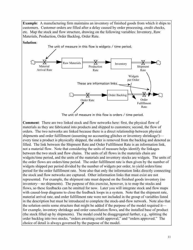
Example: A manufacturing firm maintains an inventory of finished goods from which it ships to customers. Customer orders are filled after a delay caused by order processing, credit checks, etc. Map the stock and flow structure, drawing on the following variables: Inventory, Raw Materials, Production, Order Backlog, Order Rate. Solution:

Comment: There are two linked stock and flow networks here: first, the physical flow of materials as they are fabricated into products and shipped to customers; second, the flow of orders. The two networks are linked because there is a direct relationship between physical shipments and order fulfillment (assuming no accounting glitches or inventory shrinkage!)—every time a product is physically shipped, the order is removed from the backlog and denoted as filled. The link between the Shipment Rate and Order Fulfillment Rate is an information link, not a material flow. Note that considering the units of measure helps identify the linkages between the two stock and flow chains. The units of all flows in the materials chain are widgets/time period, and the units of the materials and inventory stocks are widgets. The units of the order flows are orders/time period. The order fulfillment rate is then given by the number of widgets shipped per period divided by the number of widgets per order, to yield orders/time period for the order fulfillment rate. Note also that only the information links directly connecting the stock and flow networks are captured. Other information links that must exist are not represented. For example, the shipment rate must depend on the finished goods inventory (no inventory—no shipments). The purpose of this exercise, however, is to map the stocks and flows, so these feedbacks can be omitted for now. Later you will integrate stock and flow maps with causal-loop diagrams to close the feedback loops in a system. Note that the shipment rate, material arrival rate, and order fulfillment rate were not included in the group of variables listed in the description but must be introduced to complete the stock-and-flow network. Note also that the solution omits some structure that might be added if the purpose of the model required it—for example, inventory shrinkage and order cancellation flows, and the installed base of product (the stock filled up by shipments). The model could be disaggregated further, e.g., splitting the order backlog into two stocks, “orders awaiting credit approval,” and “orders approved.” The choice of detail is always governed by the purpose of the model.

Widgets

per Order

Order

Fulfillment

Rate

Order Rate

Shipment

Rate

Production

Rate

Material

Arrival Rate

Order Backlog

InventoryRaw Materials

The unit of measure in this flow is widgets / time period.

The unit of measure in this flow is orders / time period.

These are information links.

   

12

B1. A computer manufacturer maintains a large call center operation to handle customer inquiries. Customers with questions or problems call a toll free number for help. In this firm, incoming calls are answered by a voice recognition system that routes calls, based on the customer’s choice, either to an automated system or to a live customer service agent (CSA). Callers choosing to work their way through the automated help process can, at any time, press “0” to speak to an agent, or, of course, hang up. Callers electing to speak to a CSA may be placed on hold until an agent becomes available. If the call is answered before the customer gets frustrated and hangs up, the CSA may be able to resolve the issue. Often, however, the CSA is unable to solve the problem and forwards the call to a supervisor or specialized department such as technical support. The issue may or may not be resolved by these specialists. Map the stock and flow structure of calls as they flow through the system.

In reality, customer inquiries arrive by phone, by email, and by live chat from the firm’s website. You don’t need to consider these channels separately. Likewise, do not attempt to separate inbound calls into different categories such as billing problems or tech support questions. Assume there is a single flow of calls coming in to the system. These calls are then divided into those electing the automated system and those electing to speak to an agent.

B2. The ability of the firm above to answer calls quickly depends on the size and skill of their

CSA staff. Map the stock and flow structure for the number of CSAs. In mapping the stocks of CSAs, distinguish between “generalists” and “specialists”. Generalists are the front line agents who initially field calls; specialists are the tech support and other more highly trained people who handle the more complex inquiries generalists are unable to resolve. Call center work is stressful and turnover among both types of CSAs is high. Further, new hires are inexperienced and less productive; these are known in the firm as “rookies.” Many rookies quit before they become experienced. The firm does not hire into specialist CSA positions from outside; rather, they promote some of the experienced generalists into the better-paid specialist positions. Such firms maintain many call centers around the world (Dell, for example, has

roughly 27,000 CSAs located in dozens of call centers around the world). However, you should aggregate all such centers into a single category.

B3. Map the stock and flow structure for the adoption and diffusion of new products. To

provide a concrete context, consider the adoption of DVD players in the United States. Initially, before DVDs and DVD players were developed, everyone in the US was unaware that such an innovation existed. After DVD players were introduced to the market, people moved through various stages. Some gradually became aware of the product. Some may then enter the market (actively seeking information about different models, prices and features). Some of these people decide to buy a unit, thus becoming an adopter of the innovation. Many adopters are happy with their purchase; they may even replace their first units when they are lost, wear out, or become obsolete. Other people may decide they don’t get enough benefits from the product and don’t replace their initial units, or abandon the DVD if a better product is introduced to the market (e.g., Blu-Ray). Such individuals become former adopters.

   

13

Map two distinct stock and flow chains. The first tracks the flows of people as they move from being unaware through awareness, adoption, and, perhaps, abandonment. The second should track the flows of DVD player purchases and discards. The installed base of a product, while related to the number of adopters, can have different dynamics.

Show, using information links, how the two stock and flow chains are connected. Specifically, show how purchases and discards are related to the stocks and flows of people as they move from being unaware to adoption.

Challenge the clouds. What happens to the old units people discard?

C. Dynamics of Accumulation Stocks are accumulations. The difference between the inflows and outflows of a stock accumulates, altering the level of the stock variable. The process of accumulation gives stocks inertia and memory and creates delays. Since realistic models are far too complex to solve with formal analysis, it is important to understand the relationship between flows and the behavior of stocks intuitively. The goal is to develop your intuition about stocks and flows. Be sure to read Chapter 7

first.

C1. Consider the following system:

The top graph on the next page shows the behavior of the inflow and outflow for the stock. On the graph provided below, draw the trajectory of the stock given the inflow and outflow rates shown. Indicate the numerical values for any maxima or minima, and for the maximum or minimum values of the slope for the stock. Assume the initial quantity in the stock is 100 units.

Stock

Inflow Outflow

   

14

0

25

50

75

100

0 5 10 15 20

Units/Time

Outflow

Inflow

Time

0

50

100

150

200

250

0 5 10 15 20

Units

Time

   

15

D. Linking stock and flow structure with feedback Now we will simulate a simple stock flow system with feedback. Build and simulate a simple model of the US national debt and budget deficit. ☛ Follow the instructions below precisely. Do not add structure beyond that specified. ☛ Begin the simulation of the model in 1988 so that there is some replication of history. In

Vensim, Select Settings… under the Model menu. Then set the Initial Time = 1988, Final Time = 2088, and Time Step = 0.0625 years. Check the box to save the results every Time Step. Finally, set the unit of measure for time to Years.

☛ To keep your model simple: • Your model should have a single stock, the National Debt. The debt accumulates the Net

Federal Deficit. The only flow altering the debt is the net deficit (do not represent the issuance and maturity of the debt). In 1988 the national debt was approximately $2.5 trillion (2.5E12).

• The net federal deficit is the difference between Government Expenditure and Government Revenue.

• Government Revenue is exogenous and constant. In 1988, revenue was approximately $900 billion/year (900E9).

• Government Expenditure consists of Interest paid on the debt and Expenditures on Programs (all non-interest expenditures).

• Expenditures on Programs are exogenous and constant. In 1988 expenditures on programs were about $900 billion/year, about the same as Revenue.

• Interest payments are the product of the debt and the interest rate.

• The interest rate is exogenous and constant. In 1988 the average interest rate on the debt was approximately 7%/year (.07/year).

☛ As always, document your model and make sure every equation is dimensionally consistent. Answer the following questions.

a. What kind of feedback loop is created in your model?

b. What is the initial deficit (given the base case parameters)? c. How long does it take for the deficit to double?

d. What is the relationship between the doubling time and the interest rate? (To discover a relationship, you may want to simulate with extreme interest rates—say, between 1% per year and 15% per year).

e. Hand in your model (diagram and equation listing) and answers to the above questions. You need not hand in plots, but you should describe briefly how you arrived at your answers.

   

16

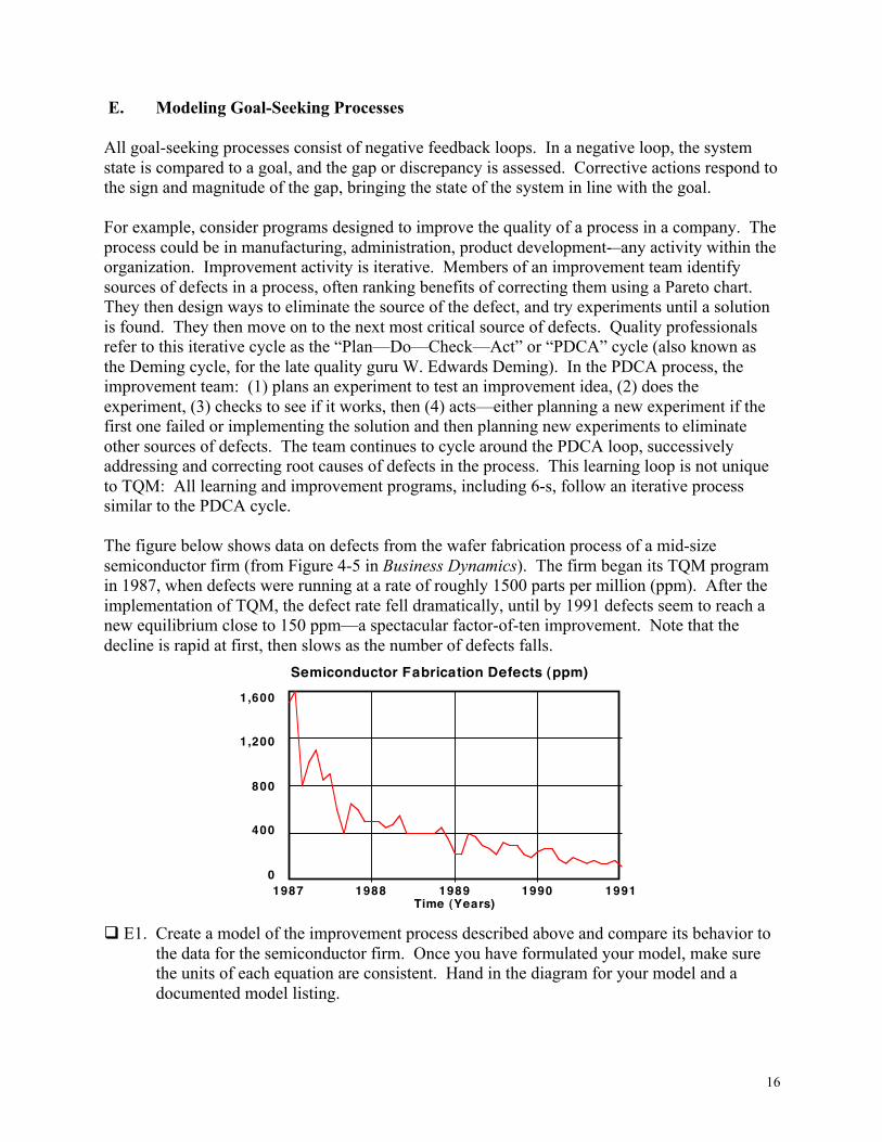
E. Modeling Goal-Seeking Processes All goal-seeking processes consist of negative feedback loops. In a negative loop, the system state is compared to a goal, and the gap or discrepancy is assessed. Corrective actions respond to the sign and magnitude of the gap, bringing the state of the system in line with the goal. For example, consider programs designed to improve the quality of a process in a company. The process could be in manufacturing, administration, product development-–any activity within the organization. Improvement activity is iterative. Members of an improvement team identify sources of defects in a process, often ranking benefits of correcting them using a Pareto chart. They then design ways to eliminate the source of the defect, and try experiments until a solution is found. They then move on to the next most critical source of defects. Quality professionals refer to this iterative cycle as the “Plan—Do—Check—Act” or “PDCA” cycle (also known as the Deming cycle, for the late quality guru W. Edwards Deming). In the PDCA process, the improvement team: (1) plans an experiment to test an improvement idea, (2) does the experiment, (3) checks to see if it works, then (4) acts—either planning a new experiment if the first one failed or implementing the solution and then planning new experiments to eliminate other sources of defects. The team continues to cycle around the PDCA loop, successively addressing and correcting root causes of defects in the process. This learning loop is not unique to TQM: All learning and improvement programs, including 6-s, follow an iterative process similar to the PDCA cycle. The figure below shows data on defects from the wafer fabrication process of a mid-size semiconductor firm (from Figure 4-5 in Business Dynamics). The firm began its TQM program in 1987, when defects were running at a rate of roughly 1500 parts per million (ppm). After the implementation of TQM, the defect rate fell dramatically, until by 1991 defects seem to reach a new equilibrium close to 150 ppm—a spectacular factor-of-ten improvement. Note that the decline is rapid at first, then slows as the number of defects falls.

E1. Create a model of the improvement process described above and compare its behavior to

the data for the semiconductor firm. Once you have formulated your model, make sure the units of each equation are consistent. Hand in the diagram for your model and a documented model listing.

Semiconductor Fabrication Defects (ppm)

1,600

1,200

800

400

0

1987 1988 1989 1990 1991Time (Years)

   

17

* Follow the instructions below precisely. Do not add structure beyond that specified.

• The state of the system is the defect rate, measured in ppm. The defect rate in 1987 was 1500 ppm.

* The defect rate is not a rate of flow, but a stock characterizing the state of the system—in this case, the ratio of the number of defective dies to the number produced.

• The defect rate decreases when the improvement team identifies and eliminates a root cause of defects. Denote this outflow the “Defect Elimination Rate.”

• The rate of defect elimination depends on the number of defects that can be eliminated by application of the improvement process and the average time required to eliminate defects.

• The number of defects that can be eliminated is the difference between the current defect rate and the theoretical minimum defect rate. The theoretical minimum rate of defect generation varies with the process you are modeling and how you define “defect.” For many processes, the theoretical minimum is zero (for example, the theoretical minimum rate of late deliveries is zero). For other processes, the theoretical minimum is greater than zero (for example, even under the best imaginable circumstances, the time required to build a house or the cycle time for semiconductor fabrication will be greater than zero). In this case, assume the theoretical minimum defect level is zero.

• The average time required to eliminate defects for this process in this company is estimated to be about 0.75 years (9 months). The average improvement time is a function of how much improvement can be achieved on average on each iteration of the PDCA cycle, and by the PDCA cycle time. The more improvement achieved each cycle, and the more cycles carried out each year, the shorter the average time required to eliminate defects will be. These parameters are determined by the complexity of the process and the time required to design and carry out experiments. In a semiconductor fab, the processes are moderately complex and the time required to run experiments is determined by the time needed to run a wafer through the fabrication process. Data collected by the firm prior to the start of the TQM program suggested the 9 month time was reasonable.

• Equipment wear, changes in equipment, turnover of employees, and changes in the product mix can introduce new sources of defects. The defect introduction rate is estimated to be constant at 250 ppm per year.

E2. Run your model with the base case parameters, and hand in the plot. a. Briefly describe the model’s behavior. b. How well does your simulation match the historical data? Are the differences likely to be

important if your goal is to understand the dynamics of process improvement and to design effective improvement programs?

c. Does the stock of defects reach equilibrium after 9 months (the average defect

elimination time)? Referring to the structures in your model, explain why or why not.

   

18

E3. Experiment with different values for the average defect elimination time. What role does

the defect elimination time play in influencing the behavior of other variables? E4. The stock reaches equilibrium when its inflows equal its outflows. Set up that equation

and solve for the equilibrium defect rate in terms of the other parameters. a. What determines the equilibrium (final) level of defects? Why? b. Does the equilibrium defect rate depend on the average time required to eliminate

defects? Why/Why not? E5. Explore the sensitivity of your model’s results to the choice of the time step or “dt” (for

“delta time”). * Before doing this question, read Appendix A in Business Dynamics. a. Change the time step for your model from 0.125 years to 0.0625 years. Do you see a

substantial difference in the behavior? b. What happens when dt equals 0.5 years? Why does it behave as it does? c. What happens when dt equals 1 year? Why does the simulation behave this way?

   

19

2. Impact of demographics on performance

This section examines the impact of subject demographics on performance in both the

pre-test and post-test. To determine the extent of prior exposure to system dynamics, students

were asked whether they had played the Beer Game (Sterman 1989); 86% had. Approximately

10% had participated in a half-day workshop on climate change the author conducted in early

2008. That workshop focused explicitly on stock-flow structure and included graphical

integration exercises with climate change cover stories (Martin 2008, Sterman and Booth

Sweeney 2007); supplement Table S-1 shows this had no significant impact on performance.

Finally, students were asked if they had seen the classic department store task before; one had

and is excluded from the analysis.

Table S-1 shows the significance levels of tests of each individual demographic variable

on the fraction correct for each of the four questions in the pre-test. Considering the first two

questions, which assess whether subjects can interpret the graph, none of the demographic

variables have a statistically significant impact on the fraction correct, with the exception of

English as a native language for Q1 only (p = .044). There is, however, no plausible reason for

native language to matter for the question of when the most people left the store but not for when

the most people entered the store. On the two stock-flow questions (Q3 and Q4, most and fewest

in the store, respectively), age, work experience, English as a native language, prior experience

with the beer game, and participation in the half-day climate change workshop have no

significant effects on performance. However, there is a highly significant gender effect, with

males outperforming females (p < .0001). The degree program in which the student is enrolled

has a marginally significant effect for both questions. The highest prior degree has at best a

marginal effect on Q4 only, and the prior field of study (STEM, social science, humanities, or

architecture) has a significant effect on Q3 only. Table S-1 also shows the Spearman rank

correlations among responses on each of the pre-test questions. As one would expect, correct

responses on Q1 and Q2 are highly correlated (r = .68, p < .0001): if one cannot determine when

the most people enter the store, one is also unlikely to know when the most are leaving. Also as

   

20

expected, correct responses on the two stock-flow questions (Q3 and Q4) are highly correlated (r

= .67, p < .0001): if one cannot determine when the most people are in the store, one is also

unlikely to know when the fewest are in the store. Performance on the graphical interpretation

questions tends to improve performance on the stock-flow questions, but much more weakly, and

the impact is statistically significant only for the correlation of Q1 and Q3: the ability to read the

graph is necessary but far from sufficient to understand the stock-flow structure of the task.

Table S-1. Impact of subject demographics on pre-test performance. Entries are the significance levels (p-values) for sex, English, beer game, climate change workshop from 2-sided Wilcoxon test; for program, highest prior degree and field from Kruskal-Wallis test; for Age and Work Experience from the χ2 test of the likelihood ratio derived from univariate logistic regression. Bold values show p < .05.

Q1 Most Entering

Q2 Most Leaving

Q3 Most in Store

Q4 Fewest in Store

Age .575 .512 .541 .790

Work Exp. .858 .094 .824 .874

Sex .341 1.00 < .0001 < .0001

English .044 .299 .738 .850

Program .420 .686 .050 .063

Highest Prior Degree

.984 .534 .220 .099

Field .715 .825 .025 .161

Beer Game .292 .740 .170 .448

Climate Change Workshop

.414 .574 .915 .277

Spearman Correlations

Q1 .683 p < .0001

.153 p = .015

.098 p = .119

Q2 .210 p = .0008

.112 p =.074

Q3 .671 p < .0001

   

21

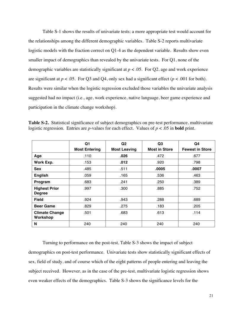
Table S-1 shows the results of univariate tests; a more appropriate test would account for

the relationships among the different demographic variables. Table S-2 reports multivariate

logistic models with the fraction correct on Q1-4 as the dependent variable. Results show even

smaller impact of demographics than revealed by the univariate tests. For Q1, none of the

demographic variables are statistically significant at p < .05. For Q2, age and work experience

are significant at p < .05. For Q3 and Q4, only sex had a significant effect (p < .001 for both).

Results were similar when the logistic regression excluded those variables the univariate analysis

suggested had no impact (i.e., age, work experience, native language, beer game experience and

participation in the climate change workshop).

Table S-2. Statistical significance of subject demographics on pre-test performance, multivariate logistic regression. Entries are p-values for each effect. Values of p < .05 in bold print.

Q1

Most Entering Q2

Most Leaving Q3

Most in Store Q4

Fewest in Store Age .110 .026 .472 .677 Work Exp. .153 .012 .920 .798 Sex .485 .511 .0005 .0007 English .059 .165 .536 .463 Program .683 .241 .250 .389 Highest Prior Degree

.997 .300 .885 .752

Field .924 .943 .288 .689 Beer Game .829 .275 .183 .205 Climate Change Workshop

.501 .683 .613 .114

N 240 240 240 240

Turning to performance on the post-test, Table S-3 shows the impact of subject

demographics on post-test performance. Univariate tests show statistically significant effects of

sex, field of study, and of course which of the eight patterns of people entering and leaving the

subject received. However, as in the case of the pre-test, multivariate logistic regression shows

even weaker effects of the demographics. Table S-3 shows the significance levels for the

   

22

demographic and other variables in a set of logistic regressions incorporating combinations of

the demographic variables, the pattern of inflow and outflow received in the post-test, and

performance on each of the four pre-test questions. As in the pre-test, there is a strong effect

gender, but the effects of age, work experience, native language, beer game experience and

participation in the climate change workshop in which stock and flow concepts were discussed

are not statistically significant in predicting success on the post-test. The effects of the degree

program in which the student is enrolled, highest prior degree, and field of study (STEM, social

science, humanities, or architecture) also were not significant.

With so many correlated regressors, the validity of the logistic regression is questionable,

so successive models eliminated variables that appeared to offer no explanatory power. The

results remain similar. Which of the eight patterns the subject received is always highly

significant, along with the impact of gender, with males outperforming females.

While the univariate Wilcoxon tests show that correctly responding on the two stock-flow

questions in the pre-test does predict post-test success, the effects are not robust in the logistic

regressions. Responding correctly on pre-test Q3 (when are the most in the store?) does improve

the odds of success in the post-test, but the effect is marginally significant. Performance on pre-

test Q4 (when are the fewest in the store?) is not significant. As a final test, Table S-3 also

reports tests the extent to which those getting both pre-test Q1 and Q2 correct, and/or Q3 and Q4

correct, predicts post-test performance. As expected, the impact of getting both graph

interpretation questions correct is not significant. Getting both Q3 and Q4 correct, indicating

those with the best grasp of stock-flow concepts, does predict post-test performance slightly, but

the effect is not statistically significant.

   

23

Table S-3. Determinants of performance on graphical department store task. Univariate p-values from logistic regression for Age and Work Experience, from nonparametric tests (Wilcoxon or Kruskal-Wallis) for all other variables.

Post-test, % incorrect Univariate

effects (p) Logistic Regression (p)

Age .775 .338 Work Exp. .762 .801 Sex .003 .017 .027 .051 .032 .017 .017 English .534 .803 Program .201 .866 .916 Highest Prior Degree

.131 .835 .664

Field .039 .368 .431 Beer Game

.853 .443

Climate Change Workshop

.563 .868

Condition (1-8)

< .0001 .004 .003 .001 .002 .002 .002

Pre-test Q1 correct

.256 .223 .401 .270

Pre-test Q2 correct

.355 .349 .512 .371

Pre-test Q3 correct

.002 .076 .083 .054 .057

Pre-test Q4 correct

.002 .836 .786 .852 .854

Pre-test Q1 and Q2 correct

.512

Pre-test Q3 and Q4 correct

.110 .081