Supp ort - ma.huji.ac.il
519
Transcript of Supp ort - ma.huji.ac.il

Repeated Games
Jean-François Mertens
Sylvain Sorin
Shmuel Zamir
Jean-François Mertens,
core, Université Catholique de Louvain,
34, Voie du Roman Pays,
B-1348 Louvain-la-Neuve,
Belgique.
E-mail address: [email protected]
Sylvain Sorin,
Université Paris X, Nanterre
and Laboratoire d'Économétrie de l'École Polytechnique,
1, rue Descartes,
75005 Paris,
France.
E-mail address: [email protected]
Shmuel Zamir,
Department of Statistics,
The Hebrew University of Jerusalem,
Jerusalem,
Israel.
E-mail address: [email protected]

Support of core and of numerous other institutions over the years is gratefully
acknowledged. So is Fabienne Henry's invaluable help in typing draft after draft. . .
These notes represent work in progress, and far from its nal form. An earlier version
was circulated previously, and has been cited in various places. In view of this, we felt
that the time had come to make it more widely available, in the form of discussion
papers. We hope eventually to publish it in a more polished format. Remarks and
suggestions are most welcome.
Louvain-la-Neuve, June 1993
Revised 31st July 2000.

Part A
Background Material


CHAPTER I
Basic Results on Normal Form Games
Non-cooperative games (or strategic games) are mainly studied through two models:
normal form orextensive form. The latter will be presented in ch. II. The former describes
the choice spaces of each player and the result of their common choices. This is evaluated
in terms of the players' von Neumann-Morgenstern utilities (i.e. the utility of a random
variable is its expected utility (von Neumann and Morgenstern, 1944, ch. I, 3.5)), hence
the following denition:
A normal form game is dened by a set of players I, strategy spaces Si, i 2 I, and
realpay-o functions F i, i 2 I, on S =
QiS
i.
It is nite (or a bi-matrix game if #I = 2) if I and all Siare nite.
Under suitable measurability conditions one denes the mixed extension of a game
G = (I, (Si, F i)i∈I) as the game Γ = (I, (Σi, φi)i∈I) where Σiis the set of probabilities on Si
and φi(σ) =RSF i(s)
Qi∈Iσ
i(dsi). Unless explicitly specied (or self-evident) otherwise,
the following denitions are always used on the mixed extension of the game.
si is a dominant strategy of player i if F i(si, s−i) F i(ti, s−i) for all ti in Si, and
s−i 2 S−i =Q
h=iSh.
si is dominated (resp. strictly dominated) if there exists ti with F i(ti, s−i) > F i(si, s−i)for some s−i
(resp. all s−i) and F i(ti, ) F i(si, ).
si is a (ε-)best reply to s−iif F i(si, s−i) F i(ti, s−i) (ε) for all ti 2 Si
.
An (ε-)equilibrium is an I-tuple s such that for every i, si is a (ε-)best reply to s−i.
A two-person zero-sum game (or: a matrix game if strategy sets are nite) is a
normal form game with I= fI, IIg, SI = S,SII = T , F I = g = F II. One denes then the
minmax v(g) = inft∈T sups∈S g(s, t) and the maxmin v(g) = sups∈S inft∈T g(s, t).If they are equal the game has a value v(g).s is an (ε-)optimal strategy for player I if g(s, t) v(g) (ε) for all t 2 T .
1. The minmax theorem
A minmax theorem gives conditions under which a two-person zero-sum game (S, T ; g)has a value. We allow here the pay-o function g to map ST toR. All minmax theorems
in this paragraph will be derived from Theorem 1.6. Prop. 1.8 uses additional convexity
assumptions to weaken continuity requirements, and Prop. 1.17 applies the previous result
to the mixed extension of the game.
1.a. Denitions and notations. We start by introducing basic denitions and nota-
tions.
Definition 1.1. A convex set is a convex subset of a vector space on the reals.
Definition 1.2. An admissible topologyon a convex set S is a topology such that,
for each n, and for every n tuple x1, . . . , xn of points in S, the mapping φx1,...,xn from
the n 1 dimensional simplex f p = (p1, . . . , pn) j pi 0,Pn
i pi = 1 g to S, that maps p
3

4 I. BASIC RESULTS ON NORMAL FORM GAMES
toPn
i=1 pixi, is continuous, when the simplex is endowed with its usual topology (i.e. the
topology induced by the Euclidian norm).
Definition 1.3. A convex topological space is a convex set endowed with an admiss-
ible topology.
Remark 1.1. Any convex subset of a linear topological (or: topological vector) space
is a convex topological space.
Remark 1.2. A compact space is not assumed to be Hausdor (T2), unless explicitlystated.
Definition 1.4. For a topological spaceS, a function f : S ! R[f1g is upper se-mi-continuous (u.s.c.) i ff xg is closed for every x. f is lower semi-continuous
(l.s.c.) i (f) is u.s.c.Remark 1.3. On a completely regular space, the u.s.c. functions that are bounded
from above are the inma of a family of bounded continuous functions.
Definition 1.5. For a convex set S, f : S ! R is quasi-concave i ff xg is
convex for every x. f is quasi-convex i (f) is quasi-concave. f is concave (resp.
convex, ane) i f(αx1+(1α)x2) αf(x1)+ (1α)f(x2) (resp. , =) whenever theright hand member is well dened (0 < α < 1).
1.b. A basic theorem.
Theorem 1.6. (Sion, 1958) Assume S and T are convex topological spaces, oneof which is compact. Assume that, for every real c, the sets f t j g(s0, t) c g andf s j g(s, t0) c g are closed and convex for every (s0, t0) 2 S T . Then
sups∈S
inft∈Tg(s, t) = inf
t∈Tsups∈Sg(s, t) .
If S (resp. T ) is compact, then sup (resp. inf) may be replaced by max (resp. min), i.e. thecorresponding player has an optimal strategy.
Proof. Obviously, one always has
sups∈S
inft∈Tg(s, t) inf
t∈Tsups∈Sg(s, t) .
Suppose therefore, in contrary to the theorem that, for some real number c,
sups∈S
inft∈Tg(s, t) < c < inf
t∈Tsups∈Sg(s, t) .
Assume, for instance, that S is compact. The sets At = f s 2 S j g(s, t) < c g form an
open covering of S; thus, there exist t1, . . . , tn such that the sets Ati (1 i n) cover S:We can restrict T to the convex hull of the set T0 of points ti (1 i n) and work now
on the (n 1)-simplex, using the admissibility of the topology. All our assumptions are
still valid. We can now do the same operation with the sets Bs = f t 2 T j g(s, t) > c g, sothat both S and T become simplices with vertex sets S0 and T0, and with the property
that, for any s 2 S, there exists t 2 T0 such that s 2 At and that, for any t 2 T , thereexists s 2 S0 such that t 2 Bs. We can further assume that S0 and T0 are minimal for
this property, eliminating eventually some additional points from S0 and T0.Let si (1 i n) be the points in S0, and for each i, Ti = f t 2 T j g(si, t) c g. The
sets Ti are compact convex, satisfyTn
i=1Ti = ;, and, by the minimality property, for every
j,T
i=j Ti 6= ;. The next lemma will show that this implies thatSn
i=1Ti is not convex.

1. THE MINMAX THEOREM 5
Thus there exists t0 2 T such that, for all i, t0 /2 Ti: we have, for each i, g(si, t0) > c,and thus, for each s 2 S, g(s, t0) > c. The same argument would show dually that there
exists s0 2 S such that, for each t 2 T , g(s0, t) < c; we thus have both g(s0, t0) < c, andg(s0, t0) > c, the desired contradiction.
The replacement of sup by max is possible due to the upper semi-continuity of g(, t)on the compact set S (for each t 2 T ).
To complete the proof, we shall thus prove the following lemma:
Lemma 1.7. Let Ti (1 i n) be compact convex subsets of a Hausdor locallyconvex topological vector space, such that T =
SiTi is convex and such that, for every i,T
h=iTh 6= ;. Then TiTi 6= ;.
Remark 1.4. For a simpler and more general result, cf. ex. I.4Ex.19 p. 48. Here the
only sport is to obtain theorem 1.6 using just the separation theorem and in fact
only for polyhedra in nite dimensional space.
Proof. The proof goes by induction on n. We assume that the lemma is proved up
to n 1, and is false for n. ThenT
i<nTi and Tn are two disjoint compact convex sets,
and can therefore, by the Hahn-Banach theorem (cf. 1.e p. 8), be strongly separated by
a closed hyperplane, whose (compact convex) intersection with T we denote by T . Let
Ti = Ti \ T ; the Ti are compact convex, Tn = ;, and Si<n Ti = T .Further, for any j < n,
Ti/∈n,jTi, which is convex, has, by assumption, a non-empty
intersection both with Tn and withT
i<nTi, which lie on opposite sides of the hyper-
plane; therefore,T
i/∈n,jTi has a non-empty intersection with the hyperplane. ThusTi/∈n,j Ti 6= ;.It follows by the validity of the lemma for n1 that
Ti<n Ti 6= ;, i.e. (
Ti<nTi)\ T 6= ;;
this yields the contradiction.
1.c. Convexity.
Proposition 1.8. Assume S is a compact convex topological space, T is a convexset, and, for every real c, and for every (s0, t0) 2 S T , the sets f s 2 S j g(s, t0) c g areclosed and convex, and g(s0, t) is convex in t, and g < +1. Then
maxs∈S
inft∈Tg(s, t) = inf
t∈Tmaxs∈Sg(s, t).
Proof. As in the proof of the theorem, we can reduce the discussion to the case
where T is a simplex with vertices (t1, . . . , tk) and where
sups∈S
infig(s, ti) < c < inf
t∈Tsups∈Sg(s, t) .
Then, for every s 2 S, the function g(s, ) is continuous on the interior of the simplex T ,being convex. If tni are interior points, limn→∞ tni = ti, then, for every s, limn→∞ g(s, tni ) g(s, ti) by the convexity of g. Therefore, the sets Ai,n = f s j g(s, tni ) < c g, 1 i k,n = 1, 2, . . ., form an open covering of S; extracting a nite subcovering, we see that we
can replace T by some compact polyhedron T contained in the interior of T : now we have
the continuity and convexity in t of f(t, s) for every s 2 S, and we can apply theorem 1.6
p. 4 to yield a contradiction.

6 I. BASIC RESULTS ON NORMAL FORM GAMES
1.d. Mixed strategies.
Definition 1.9. A regular measure on a topological space X is a positive bounded
measure µ on the Borel sets (σ-algebra generated by the open sets) such that µ(A) =supfµ(B) j B A , B closed and compactg. Its support is the smallest closed subset
with negligible complement. The set of those measures which have total mass 1 is denoted
by ∆(X).
Definition 1.10. ∆(X) is endowed with the weak topology dened as the weakest
topology for which the mapping µ 7! µ(f) =Rfdµ is u.s.c. for all bounded u.s.c. f .
Definition 1.11. f : X ! Y is Lusin-measurable if 8ε > 0, 9K closed, compact
with µ(K) > 1 ε and f|K continuous.
Remark 1.5. The regularity of a measure is equivalent to the Lusin-measurability of
all Borel maps with values in separable metric spaces.
Proposition 1.12. ∆(X) is always T1, and is Hausdor, resp. compact, resp. comple-tely regular, if X is so. Further, if X is completely regular, the above denition coincideswith the usual one using the integral of bounded continuous functions.
Proof. For the T1 property, i.e. points are closed: If µ1 6= µ2, by regularity
there exists an open set O with µ1(O) > t > µ2(O) and µ2 does not belong to
W (µ1) = fµ j µ(O) > t g. For the Hausdor property, assume µ1 6= µ2. Given a Borel set B with
µ1(B) > µ2(B), choose (regularity) two compacts C1 (included in B) and C2 (inits complement) satisfying µ1(C1) + µ2(C2) > 1. Then there exist disjoint open
sets Oi, Ci Oi, i = 1, 2 and real numbers αi, α1 + α2 > 1 with µi(Oi) > αi.
Thus the following are disjoint neighbourhoods: Vi(µi) = fµ j µ(Oi) > αi g. For the compactness, cf. ex. I.1Ex.10 p. 13.
For the completely regular case, the above remark (sub 1.a p. 3) on u.s.c. func-
tions implies that it is enough to show thatRf dµ = inff
Rg dµ j g continuous,
bounded and above f g. This in turn follows from the fact that f is Lusin-mea-
surable and from Dini's theorem.
Proposition 1.13. (Dudley, 1968) If X is metrisable and separable, so is ∆(X)with the metric d(µ, ν) = supf jµ(f) ν(f)j j f Lipschitz with constant 1 and boundedby 1 g. Moreover if X is complete, so is ∆(X).
For more properties, cf. App.9.
Fubini's Theorem 1.14. Given positive bounded regular measures µ1 and µ2 on twotopological spaces E1 and E2, there exists a unique regular measure µ on E = E1 E2such that µ(K1K2) = µ1(K1)µ2(K2) for any closed compact subsets Ki of Ei, and thenfor any non-negative µ-measurable function f on E1E2,
RE2fdµ2 is µ1-measurable andR
fdµ =Rdµ1
Rfdµ2.
Proof. For existence, extract an increasing sequence of closed compact subsets Cni
from Ei that carry most of the mass. Let µni be the corresponding restriction of µi. By
the validity of the theorem in the compact case (Mertens, 1986a, prop. 2), we obtain cor-
responding regular measures µn = µn1 µn2 on Cn = Cn1 Cn
2 E. Clearly the µni are
increasing, so their limit µ is a regular measure on E for which our condition is easily
veried. For any such µ, observe that the regularity of µ1 and µ2 imply then the validity

1. THE MINMAX THEOREM 7
of our product formula when the Ki are µi measurable. Hence the product E1 E2 ofthe σ-elds Ei of µi-measurable sets is contained in the µ-measurable sets and µ coincides
with the product measure there. It follows immediately that µ is uniquely determined on
closed compact subsets of E, since those have a basis of neighbourhoods (regularity) thatbelong to the product of the Borel σ-elds (compactness). Therefore (regularity again),
µ is unique.
Remark 1.6. The above applied inductively yields the existence of a product also for
n factors, and the uniqueness proof remains identical, so the product is associative.
Proposition 1.15. The product of regular probabilities is a continuous map from∆(X)∆(Y ) to ∆(X Y ).
Proof. For O open in X Y and µ 2 ∆(X), f(µ, y) = µ(Oy) is l.s.c. on ∆(X) Y :choose K0 closed compact Oy0
with µ0(K0) µ0(Oy0) ε, then O1 and O2 open in X
and Y respectively with K0 O1, y0 2 O2, O1O2 O, then:lim inf
µ→µ0,y→y0
µ(Oy) lim infµ→µ0,y→y0
µ(O1)1O2(y) µ0(O1) µ0(Oy0) ε.
So f(µ, y) =Pn
i=1αi1U i up to a uniform ε, with αi > 0 and U iopen in ∆(X) Y .
Hence (Fubini) (µ ν)(O) =Rf(µ, y)ν(dy) =
Pni=1αiν(U
iµ) up to ε, and ν(U i
µ) is l.s.c.on ∆(X)∆(Y ) by our previous argument.
Proposition 1.16. Let X and Y be topological spaces, with Y Hausdor, µ be aregular measure on X and f be a Lusin-measurable function from X to Y .
(1) The image of µ by f , µ Æ f−1, is a regular measure on Y . Further if f is conti-
nuous, the mapping f from ∆(X) to ∆(Y ): µ 7! µ Æ f−1 is continuous (and alsodenoted ∆(f)).
(2) Let (Xk, ρk,) be a projective system of Hausdor spaces (ρk, : Xk ! X being thecontinuous projection for * k), with projective limit (X, ρk). Given a consist-ent sequence of regular measures µk on Xk (i.e. with ρk,(µk) = µ) there exists aunique regular measure µ on X with ρk(µ) = µk the projective limit of thesequence µk.
Proof. The rst point is clear. For the second, cf. Bourbaki (1969, 4, n03, Théorème
2).
In the sequel, we denote by Σ (resp. T ) the space ∆(S) (resp. ∆(T )), and by Tf
the space of all probability measures with nite support on T (points in Σ are mixed
strategies, points in Tf mixed strategies with nite support).
Proposition 1.17. Let S be a compact topological space, T any set. Assume that,for each t, g(, t) is upper semi-continuous in s. Then
maxσ∈Σ
infτ∈Tf
Zg(s, t) d(σ τ) = inf
τ∈Tf
maxσ∈Σ
Zg(s, t) d(σ τ).
Proof. Σ with the weaktopology is compact convex (1.12) and F (σ, τ) dened on
ΣTf by
F (σ, τ) =
Zg(s, t)d(σ τ) =
ZT
dτ
ZS
g(s, t)dσ =
ZS
dσ
ZT
g(s, t)dτ
is ane in each variable and upper semi-continuous in σ. We can therefore apply prop. 1.8
p. 5 to yield the equality.

8 I. BASIC RESULTS ON NORMAL FORM GAMES
Remark 1.7. With an appropriate redenition of regular measure the above remains
true even if S is countably compact instead of compact (Mertens, 1986a, pp. 243246, and
remark 3 p. 247).
1.e. Note on the separation theorem. The Hahn-Banach theorem was used in
the rst lemma, also in some exercises below, and in many other circumstances. Here
follows a short refresher.
In the following statements, E is a real topological vector space, all subsets considered
are convex, U denotes an open subset, and letters f linear functionals.
The basic result is
Proposition 1.18. If 0 /2 U , 9f : f(U) > 0 (f is then clearly continuous).
Proof. Apply Zorn's lemma to the open convex subsets disjoint from 0.
The basic technique for separating two convex sets is to separate their dierence from
zero. So
Proposition 1.19. If A \ U = ;, 9f : f(A) \ f(U) = ;.[With obvious renements: B has an interior point, and A is disjoint from the in-
terior of B; also: 9f 6= 0, continuous, f(A) 0 i there exists a non-empty open convexcone disjoint from A cf. I.3Ex.12 p. 37 for the necessity of the interior point.]
One can always obtain an algebraic statement from the above by using the strongest
locally convex topology dened as follows: A is radial at x 2 A i 8y 2 E, 9ε > 0: x+εy 2A; then U is open i it is radial at each of its points. So:
Proposition 1.20. If p is a sublinear functional (p(λx) = λp(x) for λ 0, p(x) 2 R,p(x+ y) p(x) + p(y)), V a subspace, f : V ! R, f(v) p(v) then 9f : E ! R, f p,f(v) = f(v) for v 2 V . (Apply 1.19 in ER to the subsets U = f (x, ϕ) j ϕ > p(x), x 2 E gand A = f (v, f(v)) j v 2 V g.)
Henceforth E will be locally convex, subsets closed, and linear functionals continuous
and non-zero.
Proposition 1.21. If 0 /2 A, 9f : f(A) 1.
Proof. Apply 1.19, U being a neighbourhood of zero.
Corollary 1.22. Finite dimensional convex subsets with disjoint relative interiors[i.e., their interiors in the ane subspace they generate] can be separated.
Proof. It suces to separate from zero the dierence D of their relative interiors.
E.g. by 1.20, we can assume E is spanned by D. If 0 is not in the closure of D, apply1.21; otherwise D has non-empty interior and use 1.18].
Otherwise, to apply 1.21 one needs conditions for the dierence B C of two closed
convex sets to be closed. This is true if one is compact; more generally, AB =T
ε>0 ε(Bb)does not depend on the choice of b 2 B, and is called the asymptotic cone of B; then:
Proposition 1.23. If AB \AC = f0g, and B or C is locally compact, then B C isclosed.
Proposition 1.24. Assume B and C are cones, one of them locally compact, andB \ C = f0g. Then 9f : f(B) 0, f(C) 0.

SECT. 1 . EXERCICES 9
Taking for B the polar P 0 (= f b j hb, ϕi 0 8ϕ 2 P g) of some closed convex coneP in the dual, one obtains the alternative: either 9c 2 C f0g, hc, ϕi 0 8ϕ 2 P , or9ϕ 2 P f0g, hc, ϕi 0 8c 2 C and this alternative holds thus as soon as one of thecones C,C0, P, P 0 is locally compact.
Proof. Apply 1.23 to B and C b for b 2 B f0g.
Corollary 1.25. If in 1.24 both B and C are locally compact, and contain no straightlines, then 9f : f(B n f0g) > 0 > f(C n f0g).
Proof. Indeed, D = B C has then the same properties, which imply that the sets
f d 2 D j f(d) 1 g, for f in the dual, form a basis of neighbourhoods of zero in D.Choose then a f yielding a compact neighbourhood.
Exercises.
The rst series of exercises investigates the general properties of the value operator. For
short, we let, for any sets S and T , and any function g(s; t) (with values in R [ f+1g or in
R [ f1g)v(g) = inf
τ∈Tf
supσ∈Σf
g(; ); v(g) = supσ∈Σf
infτ∈Tf
g(; );
where g(; ) =Rg(s; t)d( ) and we write v(g) when they are equal. We start for the record
with the obvious properties.
1. v v and both are positively homogeneous of degree one (i.e., v(tg) = tv(g) fort 0), monotone and invariant under translation by constant functions (i.e., v(g+) = v(g)+).The latter two properties imply they are non-expansive, i.e. jv(f) v(g)j kf gk with
kf gk = sups,t jf(s; t) g(s; t)j (and with the convention j1 1j = 0).
2.
a. Under the assumptions of prop. 1.17 p. 7, the common valued asserted there equals v(g).We will then use the notation (g) for f 2 j g(; t) v(g) 8t 2 T g (and similarly for T (g)under dual assumptions). (g) is closed (hence compact), convex and non-empty.
b. If a decreasing net gα satises the assumptions of prop. 1.17, then
(1) g = lim gα does also
(2) v(g) = lim v(gα)(3) If α 2 (gα) or if only gα(α; t) v(g) "α8t 2 T , with "α ! 0 then for any
limit point of α we have 2 (g).(4) If 2 Tf is "-optimal for g, it is also so for all gα with suciently large.
Hint. 1 is obvious, and 2 and 3 follow from the fact that if fα is a decreasing net of real valued
u.s.c. functions on the compact space S converging to f , and σα s.t. fα(σα) ≥ λ− εα with εα → 0, thenf(σ) ≥ λ for any limit point σ. This follows in turn from the upper semi-continuity of the fα on the
compact space Σ, and from fα → f on Σ.
3. Continuity. Let S and T be compact. Denote by C the convex cone of real valued
functions on S T , which are u.s.c. in s and l.s.c. in t. If fα is a net in C, let
'α0(s0; t0) = lim sups→s0
supα≥α0
fα(s; t0)
;
α0(s0; t0) = lim inft→t0
inf
α≥α0
fα(s0; t)
:
Dene the following concept of convergence on C: fα ! f i 'α and α converge point-wise to
f . Assume fα ! f .a. Then 8t;90 : 'α(s; t) < +1; 8s 2 S and 8 0, and similarly for .

10 I. BASIC RESULTS ON NORMAL FORM GAMES
b. The convergence is compatible with the lattice structure and with the convex cone struc-
ture:
(1) fα ! f and gα ! g imply fα ^ gα ! f ^ g, fα _ gα ! f _ g, and fα+ gα ! f + g.(2) α 0; α ! , and fα ! f imply αfα ! f .
Hint. For 2, it suces to prove e.g. convergence from above, and hence to x t0 ∈ T . Using
I.1Ex.3a, subtract then an appropriate constant to reduce (by (1) to the case where fα(s, t0) ≤ 0 ∀α, ∀s.Let µα0 = infα≥α0λα: then µαϕα(s, t0) are u.s.c., ≥ λαfα(s, t0), and decrease to λf(s, t0).
c. Assume v(f) exists and fα ! f . Then
(1) v(fα) and v(fα) converge to v(f).(2) Any limit point of "α-optimal strategies for fα ("α ! 0) belongs to (f).(3) Any "-optimal strategy with nite support for f is so for all fα ( suciently large).
Hint. Point 1 allows to use I.1Ex.2b p. 9.
d. If S and T are Hausdor (or just locally compact, i.e., such that every point has a
basis of compact neighbourhoods), the convergence concept is topological i.e., derives from a
locally convex Hausdor topology on C.
Hint. Take as subbase of open sets the sets Vt,λ,K = g ∈ C | g(s, t) < λ for s ∈ K and
Ws,λ,K′ = g ∈ C | g(s, t) > λ for t ∈ K ′ with λ ∈ R, K and K ′ compact.
4. I.1Ex.3b shows that f iα ! f i, iα ! i, iα 0 implies
Pn1
iαf
iα !
Pn1
if i. Even under
the best circumstances, the restriction to iα 0 cannot be dispensed with:
a. Let S = fs0g, T = [0; 1], f1(t) = 1t>0, f2(t) = t−1 for t > 0, f2(0) = 0: f1 and f2 belongto C and are 0, also f1+ "f2 belongs to C for " > 0 but not for " = 0: we have a monotone
straight line whose intersection with C is not closed.
b. Consider gε = (1 "f2)2 = (1 2"f2 + "2f3): this is a nice curve in a xed plane, with
this time gε 2 C for all " 0. Yet v(gε) = 0 for " > 0, v(g0) = 1.
c. Nevertheless, prove that the intersection of C with a nite dimensional ane function
space A is closed, and that on this intersection the convergence in C coincides with the usual in
A, if any dierence of two functions in A is separately bounded (i.e., bounded in each variable,
the other being xed).
5. To show that monotonicity and compactness in ex. I.1Ex.2 cannot be dispensed with:
a. Let S = N, T = f0g, gk = 1k: the gk are a sequence of positive continuous functions
converging weakly to zero (Pgk 1), yet v(gk) = 1 does not converge to zero.
b. On any innite compact Hausdor space S, the above example can be reduplicated (thus:
gk continuous, kgkk = 1, gk 0, gk(s) > 0) gn(s) = 0 8n 6= k).
Hint. Show that one can nd in S two disjoint compact sets with non-empty interior, one of which
is innite, and use this inductively.
c. Even with monotonicity, one cannot dispense with compactness: e.g., S = N, gk(n) =1n≥k.
d. Cf. also ex. II.2Ex.1 p. 84.

SECT. 1 . EXERCICES 11
6. Dierentiability. We keep the notation of ex. I.1Ex.3. Denote by G the convex cone of
functions g having a non-ambiguous, u.s.c.-l.s.c. extension g(; ) to T i.e., g(s; ) < +1is u.s.c. on S for each , g(; t) > 1 is l.s.c. on T for each , andZ
g(s; )(ds) =
Zg(; t)(dt) for each (; ):
Let also V = f f 2 C j v(f) exists g.For f 2 V , g 2 G, g|Σ(f)×T (f) 2 V (e.g. by theorem 1.6); denote the value of this game by
vf(g). We rst deal with dierentiability along straight lines, then along dierentiable curves.
Comment 1.8. Theorem 1.6 p. 4 and prop. 2.6 p. 17 give sucient conditions for f 2 V .Ex. I.1Ex.7 p. 12 and ex. I.2Ex.1 p. 20 give sucient conditions for g 2 G.
a. For f + "g 2 V , g 2 G, limε>→0[v(f + "g) v(f)]=" = vf(g).
Hint. (cf. Mills, 1956). For τ ∈ T (f), σε an ε2-optimal strategy with nite support in f + εg, onehas v(f + εg) ≤ f(σε, τ ) + εg(σε, τ ) + ε2 so (v(f + εg) − v(f))/ε ≤ g(σε, τ ) + ε. g ∈ G implies then
lim supε>→0(v(f+εg)−v(f))/ε ≤ maxσ g(σ, τ ) where σ ranges over the limit points of σε. Ex. I.1Ex.3b and
I.1Ex.3c p. 10 implies σ ∈ Σ(f). Thus lim supε>→0(v(f + εg) − v(f))/ε ≤ minτ∈T (f) maxσ∈Σ(f) g(σ, τ ) =vf(g).
b. If f + "g is real valued and satises the assumptions of theorem 1.6 for 0 " "0 (e.g.is concave in s and convex in t), one does not need g 2 G: the above argument goes through in
pure strategies, interpreting in the result (f) and T (f) as pure strategy sets.
Hint. Since Σ(f) and T (f) are compact convex, (f + εg)|Σ(f)×T (f) also satises the assumptions
of theorem 1.6. But f is constant on Σ(f)× T (f), so g|Σ(f)×T (f) satises them. Let now h = f + ε0g,and use the arguments of I.1Ex.6a for f + εh, plus the above remark and homogeneity.
c. Assume that hε 2 V and (hε h0)="! g 2 G, in the sense that, like in ex. I.1Ex.3 p. 9,
there exists, for each and , 'ε(s; ) u.s.c. in s and decreasing to g(s; ) and ε(; t) l.s.c. in tand increasing to g(; t) such that hε(s; ) h0(s; )+"'ε(s; ) and hε(; t) h0(; t)+" ε(; t).Then
v(hε) v(h0)
Æ"! vh0(g).
Hint. Argue like in I.1Ex.6a.
d.
One can use in I.1Ex.6c the homogeneity as was done sub I.1Ex.6b, using the condi-
tions hε(s; ) (1 "A)h0(s; ) + "'ε(s; ) and hε(; t) (1 "A)h0(; t) + " ε(; t)(A arbitrary) instead of the above with A = 0, and obtaining then (v(hε) v(h0))="!vh0(g) Av(h0) [since h0(; ) is not necessarily dened, even on h0 Th0, one does
not obtain as sub I.1Ex.6b that this limit equals vh0(g Ah0)]. Similarly, I.1Ex.6b can be extended: if fε satises the assumptions of theorem 1.6 p. 4
for 0 " < "0, and if for A suciently large, (fε f0)="+Af0! g+Af0 (in the sense
of ex. I.1Ex.3), then [v(fε) v(f0)]="! vf0(g).
e. In fact, closer inspection of the proof shows that much less is needed: assume fε(s; t) andg(s; t) are real valued, such that fε(0 " < "0) satises the assumptions of theorem 1.6, and
such that (letting O denote an open set):
8t; 8s0; 8Æ > 0; 9"0 > 0; 9O : s0 2 O S; 9A > 0 : 8s 2 O; 8" < "0
[fε(s; t) f0(s; t)]=" < g(s0; t) +A[maxxf0(x; t) f0(s; t)] + Æ
and the dual condition. Then g|S(f0)×T (f0) satises the assumptions of theorem 1.6, and
[v(fε) v(f0)]="! vf0(g).

12 I. BASIC RESULTS ON NORMAL FORM GAMES
Hint. Establish rst the rst statement, next that fε → f0 (ex. I.1Ex.3), next that there exist
ϕε,A(s, t) which are u.s.c. in s, decreasing in ε (ε→ 0) and A(A→ +∞), such that (fε(s, t)−f0(s, t))/ε+Af0(s, t) − Av(f0) ≤ ϕε,A(s, t), and such that for t ∈ T (f0) lim ε→0
A→+∞ϕε,A(s, t) ≤ g(s, t). Finally show
[v(fε)− v(f0)]/ε ≤ [fε(sε, t)− f0(sε, t)]/ε+Af0(sε, t)−Av(f0), for εA ≤ 1, t ∈ T (f0) and sε ∈ S(fε), andargue as above.
Comment 1.9. Thus I.1Ex.6e is by far the best result, and I.1Ex.6c and I.1Ex.6d should
be applied only in cases where I.1Ex.6e is not applicable, a.o. because the mixed extension of
the game is not dened or lacks the proper u.s.c.-l.s.c. properties. The next exercise shows such
cases are bound to be very rare.
7. Let S and T be compact metric spaces, f a bounded real valued function on ST such
that f(; t) is u.s.c. for each t and f(s; ) l.s.c. for each s.a. Show that f is Borel measurable. [Hence f(; ) is unambiguous, also the assumptions
of prop. 2.6 p. 17 are satised.]
Hint. Find an increasing sequence of functions converging point-wise to f , where for each function inthe sequence there is some partition of T with the function being constant in t on each partition element.
b. Show that f(; ) is u.s.c. on for each 2 T and l.s.c. on T for each 2 .
Hint. Use Fubini's theorem and Fatou's lemma.
c. If measurability is known, I.1Ex.7b also follows without the metrisability assumption,
but assuming just strict semi-compactness (the closure of a subset is the set of limit points of
convergent sequences in the subset). Most compact subsets of topological vector spaces have this
property (Grothendieck, 1953).
8. Often, the result of ex. I.1Ex.6 strengthens itself in the following way. Assume e.g. we
are working on a nite dimensional subspace of games, and we know (e.g. by ex. I.1Ex.1) that
the function v is Lipschitz on this subspace. Then we have: if a Lipschitz function f : Rn ! R
is such that f ′x(y) = limε>→0f(x + "y) f(x)
=" exists for all x and y, then f ′x() is Lipschitz
and is a true dierential, i.e. F (y) = f(x+ y) f(x) f ′x(y) is dierentiable at zero (with zero
dierential: limε→0 sup0<‖y‖≤ε jF (y)j = kyk = 0).
9.
a. The Lipschitz condition in ex. I.1Ex.8 is necessary: on [0; 1]2, F (x; y) = x3y=(x4+ y2) isanalytic except at zero, is Lipschitz at zero: 0 F (x; y) 1
2 k(x; y)k, and has all its directional
derivatives zero (thus linear) at zero, yet F (t; t2) = 12 t: F is not dierentiable at zero.
b. u.s.c.-l.s.c. functions occur quite easily, e.g. on [0; 1]2 : F (0; 0) = 0, F (x; y) = (yx)=(y+x).
c. The boundedness condition in I.1Ex.7b is really needed: even with separate continuity
(where the metrisability condition in ex. I.1Ex.7 become superuous, cf. ex. I.2Ex.1 p. 20), dene
F on [0; 1]2 by F (0; 0) = 0, F (x; y) = xy=(x3+y3). Show that the mixed extension (which always
exists by I.1Ex.7a using just positivity), although being jointly lower semi-continuous (F being
so), is not separately u.s.c.
Show also that, for real valued measurable functions, boundedness of the function is equival-
ent to niteness of the mixed extension (i.e., (absolute) integrability for every product probabil-
ity).

2. COMPLEMENTS TO THE MINMAX THEOREM 13
10. Compactness of (X) for compact X. (Mertens, 1986a)
Denote by C the convex cone of bounded l.s.c. functions on a compact space X and let
E = C C. Denote by P the set of monotone functions on C satisfying
p(tf) = tp(f) for t 0 and
p(f + g) p(f) + p(g).
P is ordered in the usual way. Let M(X) be the set of minimal elements of P .a. 8p 2 P , 9 2M(X) : p.
Hint. Given α ≤ 0, f ≥ α and q ≤ p, one has p(f) ≥ q(f) ≥ q(α) ≥ −q(−α) ≥ −p(−α), hence theset of possible values for q(f) is a bounded interval use Zorn.
b. Any in M(X) can be identied with a positive linear functional on E satisfying:
(f) = inff(g) j g 2 C; g f g:Hint. µ dened by the above right hand member satises i) and ii) and coincides with µ on C. Use
Hahn-Banach to get a positive linear functional ζ ≤ µ. This ζ is unique otherwise µ would not be
minimal on C hence, using again Hahn-Banach, coincides with µ.
c. M(X) is the set of regular Borel measures on X.
Hint. Follows from a Daniell-type extension:
If fn is an increasing sequence in C, µ(lim fn) = limµ(fn), (use Dini, cf. (Meyer, 1966, X.6) and
I.1Ex.10b). Dene µ∗ on the set F of real bounded functions on X by µ∗(f) = infµ(g) | g ∈ C, g ≥ f .Then:
µ∗(f + g) ≤ µ∗(f ∨ g) + µ∗(f ∧ g)) ≤ µ∗(f) + µ∗(g)
and if fn is an increasing sequence in F , µ∗(lim fn) = limµ∗(fn).Dene L = f ∈ F | µ∗(f) + µ∗(−f) ≤ 0 . L is a vector space and µ∗ a linear functional on it.
Given O and U open in X, 1O and 1O∩U are in L, hence also 1O\U with: µ∗(O) = µ∗(O∩U)+µ∗(O \U),hence for any subset A: µ∗(A) ≥ µ∗(A ∩ U) + µ∗(A \ U), so that any open U is µ∗-measurable, hence allBorel sets also.
Finally since µ∗(A) = supµ(F ) | F ⊆ A, F closed , and X is compact, µ∗ denes a regular Borel
measure (unique since equal to µ on open sets).
d. For all t > 0, the sets f j 2 (X); (1) = t g and f j 2 (X); (1) t g are
closed and compact (Recall 1.12).
Hint. It suces to prove the compactness of the second set. Given an ultralter on it, let ϕ denote
its point-wise limit in the set of positive linear functionals on E. By I.1Ex.10a there exists ν ∈ ∆(X)with ν ≤ ϕ on C: ν is a limit point in ∆(X).
2. Complements to the minmax theorem
This section gives a number of more specialised how to use tricks and other comple-
ments for the minmax theorem of sect. 1 and its usual form (prop. 2.6 p. 17).
2.a. The topology on S. Since there is no Hausdor requirement, prop. 1.17 just
asks that S be compact when endowed with the coarsest topology for which the functions
f(, t) are u.s.c. This is equivalent (Mertens, 1986a, remark 1, p. 247) to ask that any
point-wise limit of pure strategies i.e. of functions f(s, ) be dominated (i.e., smaller
on T ) by some pure strategy. Using the countably compact version, this can even be
further weakened to: for any countable subset T0 of T , and any sequence si 2 S, thereexists s0 2 S such that, for all t 2 T0, lim infi→∞ f(si, t) f(s0, t) (Mertens, 1986a, remark
3, p. 247).

14 I. BASIC RESULTS ON NORMAL FORM GAMES
2.b. Lack of continuity: regularisation. Here we consider the case where the
u.s.c. or compactness condition is not met.
Definition 2.1. Let (Ω,A ) denote a measurable space, and Σ a class of probability
measures on (Ω,A ). The support function φF(σ) of a class F of extended real valued
functions on Ω is dened on Σ by
φF(σ) = inff∈F
Z
f dσ
whereRdenotes the lower integral (
Rf dσ = supf
Rh dσ j h f, h measurable and
bounded from above g).Definition 2.2. Let, for each measurable set B, FB = f f|B j f 2 F g. Denote by
co(F ) the convex hull of the set of bounded functions minorated by some element of F ,
and by m(F ) the monotone (decreasing) class generated by F : the smallest class of
functions containing F and containing the limit of every decreasing sequence in m(F ).Let nally D(F ) (or DΣ(F )) be such that:
D(F ) = f f bounded from above j 8σ 2 Σ, 9B 2 A : σ(B) = 1, f|B 2 m(co(FB)) gD(F ) stands for the decreasing class generated by F .
Lemma 2.3. D(F ) f g bounded above jRg dσ φF(σ) 8σ 2 Σ g, with equality
if:
(1) all functions inF are σ-measurable and σ-a.e. bounded from above, for all σ 2 Σ,(2) Σ contains every probability measure which is absolutely continuous w.r.t. some
σ 2 Σ.
Proof. We rst show inclusion. It suces to show that
g 2 m(co(F )) )Z
g dσ φF(σ)
(applying then this result on some set B with σ(B) = 1). This follows from the stand-
ard properties of the lower integral (note that any decreasing sequence in m(co(F )) isuniformly bounded above).
We turn now to the other inclusion. It will be sucient to prove that, for bounded gsatisfying
Rg dσ φF(σ) for all σ 2 Σ, one has g 2 D(F ), since, for any other g, one will
then have g_(n) 2 D(F ) for all n, hence, g 2 D(F ), D(F ) being a monotone class. (In
fact, assume gn 2 D(F ) decreases to g; let σ(Bn) = 1, hn 2 m(co(FBn)) : hn gn|Bn
. For
B =T
nBn, one has σ(B) = 1 and m(co(FB)) [m(co(FBn))]|B, so hn|B 2 m(co(FB))
and, for some constant K, hn|B gn|B K, so h = limk→∞ supn≥k hn|B 2 m(co(FB)) andh g|B.)
Fix now σ, and let g 2 L∞(σ) stand for the (σ-)essential supremum of the measur-
able functions smaller than g. Note that, for any non-negative measure µ in L1(σ), i.e.bounded and absolutely continuous w.r.t. σ:
Rg dµ inff∈F
Rf dµ since, by assumption,
(µ/kµk) 2 Σ.Now, if µ 2 L1(σ) has a non-zero negative part µ−, consider the Hahn decompos-
ition µ = µ+ µ−, µ+ 0, µ− 0, µ+(B−) = 0, µ−(B+) = 0, B+ and B− meas-
urable, B+ \ B− = φ. Fix f0 2 F (f0 K µ-a.e.), and let fn = f+0 + n1B−; we
have fn 2 L∞(σ), fn f0 2 F , and µ(fn) = µ(f+0 ) + nµ−(B−) ! 1. There-
fore, if G = f g 2 L∞(σ) and bounded below j 9f 2 F : f g g, we have, for all
µ 2 L1(σ),Rg dµ infG
Rg dµ. Thus, g belongs, by the Hahn-Banach theorem (1.e), to

2. COMPLEMENTS TO THE MINMAX THEOREM 15
the σ(L∞, L1)-closed convex hull of G. Denote by Gcthe convex hull of G, and by Gc,m
the monotone class spanned by Gc, i.e. the smallest class of functions containing Gc
and
such that fn 2 Gc,m, fn decreasing to f , f bounded below imply f 2 Gc,m
(thus Gc,m
consists of those functions of m(Gc) which are bounded below). Note that Gc,mis convex,
and Gc,m +L +∞(σ) Gc,m
.
Denote byH the image ofGc,min L∞(σ), i.e. the set of equivalence classes ofGc,m
. H is
still convex, H +L+∞(σ) H, and fn 2 H, supn kfnkL∞ < +1 implies lim supn→∞ fn 2 H.
Indeed, if gn 2 Gc,mbelongs to the equivalence class of fn, if M = supn kfnkL∞, if
Bn = f s j gn(s) > M g, and if hn = (supk≥n gk) _ (M), then hn decreases every-
where to some element h of the equivalence class lim supn→∞ fn, h is bounded below and
fh1 > Mg B =S
nBn. Since σ(B) = 0 and since hn gn 2 Gc,m, we have indeed
hn 2 Gc,mand thus h 2 Gc,m
, so lim sup fn 2 H.
We have seen that g belongs to the weak, i.e. σ(L∞, L1)-closure of H. We will now
show that H is weak-closed, so it will follow that g is the equivalence class of some
element g of Gc,m: there exists g 2 Gc,m
, g g except on a σ-negligible set.We want thus to show that a convex subset H of L∞ is weak
-closed if (fn 2 H,
supn kfnkL∞ < +1 implies lim sup fn 2 H). By the Krein-Smulian theorem on weak-
closed convex sets (Kelley et al., 1963, p. 212), since H is convex in the dual L∞ of the
Banach space L1, it is sucient to show that the intersection of H with any ball is weak-
closed: we can assume that supf∈H kfk∞ = R < +1. Further, it is sucient to prove
thatH is τ(L∞, L1)-closed (Kelley et al., 1963, p. 154, Th. 17.1). But the Mackey-topology
τ(L∞, L1) is ner than any Lp topology, hence a fortiori than the topology of convergence
in measure. (In fact, they coincide on bounded subsets of L∞, cf. ex. I.2Ex.12 p. 24). Sincethis topology is metrisable, and since, from any sequence that converges in probability,
one can extract an a.e. convergent subsequence, it is sucient to show that if a sequence
fn in H converges a.e. to f then f (= lim sup fn a.e.) belongs to H, which is our basic
property of H. Thus, for some g 2 Gc,m, and some measurable set B0 with σ(B0) = 1, we
have g g everywhere on B0.Note now that, given a set G of functions, the union of the monotone classes generated
by all countable subsets of G is a monotone class (because a countable union of countable
subsets is still countable), and hence is the monotone class spanned by G. Thus g belongsto the monotone class spanned by a sequence gn 2 Gc
, and each gn is a convex combinationof nitely many gn,i 2 G. Since gn,i 2 L∞(σ), there exists Bn,i 2 A with σ(Bn,i) = 1such that gn,i|Bn,i
is bounded and A -measurable. Choose also fn,i 2 F , fn,i gn,i: for
B = B0\(T
n,iBn,i), we haveB 2 A , σ(B) = 1, gn,i|B is bounded, measurable and fn,i|B:thus gn|B 2 co(FB) and g|B 2 m(co(FB)) with g|B g|B. Since such a construction is
possible for each σ 2 Σ, we have indeed g 2 DΣ(F ).
Given a function g on S T , let, for all τ 2 Tf, φτ(s) = lim sups′→s g(s′, τ), and let
D(g) = Dfφτ j τ 2 Tf g. We dene similarly I(g) (I for increasing), reversing the rôles
of S and T and the order on the reals.
Proposition 2.4. Let S be a compact topological space, T any set. Assume, for allt 2 T , g(, t) 2 D(g). Then,
maxσ∈Σ
infτ∈Tf
Zg(s, t)d(σ τ) = inf
τ∈Tf
supσ∈Σ
Zg(s, t) d(σ τ) .

16 I. BASIC RESULTS ON NORMAL FORM GAMES
Proof. Prop. 1.17 can be applied to the game φτ(s); one obtains pure strategies τbecause φτ(s) is convex in τ . The lemma yields then that the same optimal strategy σguarantees the same amount against g, hence the result.
Comment 2.1. The convexity in τ of φτ(s) implies that the convexication in the
denition of D will be superuous: one would equivalently obtain D if, instead of using
m(co(F )), one just stabilised the set of functions fφτ j τ 2 Tf g under the lim sup of
sequences which are uniformly bounded from above.
Comment 2.2. When the pay-o function g is uniformly bounded from above, as in
many applications, one does not even have to stabilise: one could equivalently just dene
G = f lim supn→∞φτn j τn 2 Tf g, and D = fh j 8σ 2 Σ, 9f 2 G : f h σ-a.e. g. Indeed,take f 2 m(co(FB)), f h|B, σ(B) = 1. Then, clearly f belongs to the closure of co(FB)for the topology of convergence in measure, i.e., since σ(B) = 1, the equivalence class of fbelongs to the closure of co(F ). Thus, f is the limit in measure of a sequence in co(F ),hence the limit of a σ-a.e. convergent sequence fn 2 co(F ). Each fn is minorated by some
φτn, hence lim supn→∞φτn h σ a.e.. Since the pay-o function is uniformly bounded
from above, the sequence φτn is also.
Comment 2.3. Further, in most actual applications (cf. exercises), the σ-a.e. aspectin the denition of D is not needed. Thus this is the form in which the criterion is
most often used: show that, for each t 2 T , there exists a sequence τn 2 Tf such that
lim supn→∞φτn() g(, t) (and such that φτn() is uniformly bounded from above if g isnot).
Comment 2.4. Only the obvious part (monotone convergence theorem)of the lemma
was needed. The hard part shows that the above simple use of the monotone convergence
theorem (or of Fatou's lemma) is as powerful as the more sophisticated closure methods,
as used for instance in (Karlin, 1950). Indeed, any such closure method will only yield
functions satisfying, for all σ,Rf dσ infτ
Rφτ dσ.
2.c. Lack of compactness: approximation. When also S is not necessarily com-
pact, the previous ideas can be combined with an old idea going back to Wald (1950):
that compactness is not really necessary, only an appropriate form of precompactness (but
in the uniform topology) and in fact a one-sided form, as was later observed.
Since, however, our typical assumptions are much weaker that a joint continuity of the
pay-o function, the typical compactness that we have is not in the uniform topology, not
even a one-sided form, so we retain from this precompactness only the one-sided uniform
approximation by another game with compact (and not necessarily nite) strategy space:
we will let the function φ vary with ε, and use compact subsets Σε of Σ.
Proposition 2.5. Assume that, for all ε > 0, there exists a compact convex subsetΣε of Σ, and a function φε : S Tf ! R [ f1g such that
(1) φε(s, τ) is u.s.c. in s and convex in τ(2) for all t 2 T , g(, t) 2 DΣε
fφε(, τ) j τ 2 Tf g(3) for all s 2 S, there exists σs 2 Σε such that g(s, τ)
Rφε(, τ) dσs + ε, for all τ .
Then
supΣ
infTf
Zg(s, t) d(σ τ) = inf
Tf
supΣ
Zg(s, t) d(σ τ)
Proof. Apply prop. 1.8 p. 5 to φε on Σε Tf; let vε, σε and τε be the correspondingvalue and optimal strategies. By 2 and lemma 2.3, σε still guarantees vε against Tf in the

2. COMPLEMENTS TO THE MINMAX THEOREM 17
game g. By 3, τε guarantees vε + ε against S in g. This being true for all ε, the value vexists and σε and τε are ε-optimal strategies.
Comment 2.5. Typically, one thinks of Σε as the set of probabilities on a compact
subset Sε of S.
Comment 2.6. The previous proposition was the particular case where σs was theunit mass at s and φε was independent of ε.
Comment 2.7. Point 3 and the compactness of Σε, together with the upper semi-
continuity of φε, imply that any limit of functions g(s, ) on Tf is ε-dominated by some
function φε(σ, ).Comment 2.8. This last condition (together with 2) is in principle sucient, barring
some measurability problems: use rst prop. 1.17 p. 7 to solve the game where player I'sstrategy set is the set of all limits of functions g(s, ). Let σ0 be his optimal strategy in this
game and v the value. If one could select in a measurable way for each limit function a σsuch that φε(σ, ) ε-dominates the function, use this selection to map σ0 to some σ0 2 Σ,which guarantees in the game φε at least v ε. By 2, σ0 will also guarantee v ε in g,hence be an ε-optimal strategy in g.
Even without such a measurable selection, one might e.g. attempt to dene a mixed
strategy as some auxiliary probability space (here σ0), together with a map from there
to the strategy space (here an arbitrary, non-measurable selection), such that player Iguarantees himself v ε in the sense of lower integrals.
2.d. Measurability: symmetric case. The right-hand member (and thus the left-
hand member) in the equality of the above propositions is not increased if Σ is replaced
by the space Σ of all order preserving linear functionals of norm 1 on the cone of functions
on S generated by the functions g(, t) and the constants. That is to say that quantity
is an unambiguous upper bound for any evaluation of the game (because symmetrically
player II's strategies are of most restricted type (nite support)). Denote by TB the set
of all probability measures on some σ-eld B on T , and let F (σ, τ) =RTdτRSg(s, t) dσ,
where the integral on T is in the sense of a lower integral. Then
maxσ∈Σ
infτ∈TB
F (σ, τ) = infτ∈Tf
supσ∈ΣF (σ, τ) .
Thus the possible discrepancy between upper and lower bound apparently depends more
on the order of integration than on the allowed strategy spaces.
Although those propositions are a basic tool in proving that a game has a value, the
above shows well why they do not assert per se that the game in question has a value:
the value might in general depend on the order of integration, or, in other terms, on the
greater or lesser generality of mixed strategies allowed for each player. The next proposi-
tions show some cases where this ambiguity can be relieved completely. (A less complete
(cf. ex. I.2Ex.11 p. 23) way of relieving it would be to add to the previous assumptions
some measurability requirement and use Fubini's theorem to obtain the minmax theorem
directly on the mixed extension). Obviously one would by far prefer to be able to dispense
with the hypotheses in the next theorem cf. (Mertens, 1986a) for the importance of
this question, and why this would yield a completely intrinsic theorem.
Theorem 2.6. Assume S and T are compact, and g is real valued and bounded frombelow or from above. Assume further that g(s, ) is lower semi-continuous on T for each

18 I. BASIC RESULTS ON NORMAL FORM GAMES
s 2 S, and g(, t) is upper semi-continuous on S for each t 2 T . Then under any one ofthe following three hypotheses:
(1) g is µ ν measurable for any regular product probability on the Borel sets ofS T ,
(2) one of the two spaces has a countable basis(3) one of the two spaces is Hausdor
one has:
supσ∈Σf
inft∈T
Zg(s, t)dσ = inf
τ∈Tf
sups∈S
Zg(s, t)dτ .
Further each player obviously has an optimal strategy in the form of a regular probability.
Proof. In case 1, prop. 1.17 p. 7 applied both ways, yields the existence of an up-
per value v, that player I can guarantee with a regular probability µ, and player IIwith probabilities with nite support, and of a lower value v, that player II can guar-
antee with a regular probability ν and player I with probabilities with nite support.RSg(s, t) µ(ds) ν implies
RTν(dt)
RSg(s, t) µ(ds) v and, similarly,
RTg(s, t) ν(dt) v
impliesRSµ(ds)
RTg(s, t)ν(dt) v. By the measurability and boundedness assumptions
of g, we can apply Fubini's theorem: v RTdνRSg dµ =
RSdµRTg dν v. But, by their
very denition v v (they are sup inf and inf supof the game played in strategies with
nite support): the proof is complete in this case.
Suppose now that 2 holds; we shall prove that in this case g is Borel so 1 applies.
Assume that T has a countable basis On, and dene:
fn(s, t) =
(1, for t /2 On
inft′∈Onf(s, t′), otherwise.
Then fn is Borel (since u.s.c. in s) and gn = maxk≤n fn is an increasing sequence convergingto f (since l.s.c. in t).
It remains to consider case 3. Hence assume T Hausdor. We will rst construct a
countable set of best replies. Let Tn = f τ 2 Tf j # Supp(τ) n g. Denote by Φ0 the set ofcontinuous functions ϕ on T such that there exists s 2 S with f(s, ) ϕ() on T . Sincev infτ∈Tn
supϕ∈Φ0
Rϕdτ , the following sets: Oϕ,k,n = f τ 2 Tn j
Rϕdτ > v 1/k g, form
for ϕ 2 Φ0 and each xed n and k, an open covering of the compact space Tn. Denote by
Φk,n the indices of a nite subcovering. Then Φ =S
k,nΦk,n is a countable subset of Φ0,
such that v = infτ∈Tfsupϕ∈Φ
Rϕdτ . We now reduce the situation to one where 2 applies.
If ϕi enumerates Φ, let us consider on T T , d(t1, t2) =P
i 2−i jϕi(t1) ϕi(t2)j / kϕik. d
denes a metrisable quotient space eT of T , such that, if ψ denotes the quotient mapping,
any ϕ 2 Φ can be written as g Æ ψ, for some g 2 Ψ, where Ψ denote the set of all g
continuous on eT , such that for some s 2 S, g Æ ψ(.) f(s, .) on T . Dene ef on S eT byef(s,et) = supf g(et) j g 2 C( eT ), g Æ ψ(.) f(s, .) g. Then we have:
v infτ∈Tf
supϕ∈Φ
Zϕdτ inf
τ∈Tf
supg∈Ψ
Zg Æ ψ(t)dτ(t) inf
τ∈Tf
sups∈S
Z ef(s,et)deτ (et).Obviously ef is l.s.c. on eT for each s 2 S, and is the largest such function satisfyingef(s, ψ(t)) f(s, t). Let h(s,et) = inff f(s, t) j t 2 ψ−1(et) g: to prove that ef is u.s.c. on
S, we will show that ef = h. This in turn follows from h(s, .) being l.s.c. on eT for each
s 2 S. In fact eT being metrisable, let eti be a sequence converging to et. Choose ti such that

2. COMPLEMENTS TO THE MINMAX THEOREM 19
ψ(ti) = eti and f(s, ti) h(s,eti)+1/i, and let t be a limit point of the sequence ti: we haveψ(t) = et and h(s,et) f(s, t) lim inf f(s, ti) lim inf h(s,eti) hence the required property.
We then use the result under case 2 for ef on S eT . It follows that v supσ∈Σfinf t∈TR ef(s,et)dσ(s) supσ∈Σf
inft∈T
Rf(s, t)dσ(s), since ef(s, ψ(t)) f(s, t). This completes
the proof of the proposition.
Remark 2.9. When g is continuous in each variable no further assumptions are
needed: either by using ex. I.2Ex.1 p. 20 to show that condition 1 is satised or reducing
to 3, by using e.g. on S the coarsest topology for which all functions g(, t) are continuous(and going to the quotient space) (cf. ex. I.2Ex.11 p. 23 for an example showing that, even
with such assumptions, compactness on both sides is really needed).
We obtain now the analogues to propositions 2.4 p. 15 and 2.5 p. 16.
Proposition 2.7. Let S and T be compact. Assume g(s, ) and g(, t) are boundedfrom below and from above resp. for all (s, t) 2 S T . Assume there also existsf : S T ! R, measurable for any regular product probability and bounded either frombelow or from above, and such that,
f(s, ) 2 I(g) 8s 2 Sf(, t) 2 D(g) 8t 2 T
Then g has a value, and both players have ε-optimal strategies with nite support.
Proof. Is the same as the proof of theorem 2.6, but using prop. 2.4 instead of
prop. 1.17
Comment 2.10. One usually takes f to be (some regularisation of) g, cf. exercises.
With the same proof as above one obtains:
Proposition 2.8. Assume, for all ε > 0, there exist compact, convex subsets Σε andTε of Σ and T and functions φε : S Tf ! R [ f1g, ψε : Σf T ! R [ f+1g,fε : S T ! R such that
(1) φε is u.s.c. in s and convex in τ ; ψε is l.s.c. in t and concave in σ;(2) fε is measurable for any regular product measure, and bounded from below or
from above;(3) for all s 2 S, there exists σs 2 Σε such that, for all τ 2 Tf,
g(s, τ) φε(σs, τ) + εand, for all t 2 T , there exists τt 2 Tε such that, for all σ 2 Σf,
g(σ, t) ψε(σ, τt) ε ;(4) fε(, t) 2 DΣε
(φε) for all t 2 T and fε(s, ) 2 ITε(ψε) for all s 2 S.
Then g has a value, and both players have ε-optimal strategies with nite support.
Comment 2.11. Theorem 2.6 and propositions 2.7 and 2.8 imply that each player has
ε-optimal strategies that are safe against any type of mixed strategy of the other player
(even nitely additive ones . . . ) no matter in what order the integrations are performed.
Further, those mixed strategies are really playable in the sense that one can obviously
realise the mixing with a nite number of coin tosses. That is why we say the game has
a value.

20 I. BASIC RESULTS ON NORMAL FORM GAMES
2.e. Pure optimal strategies.
Definition 2.9. Call a function f dened on S T concave-like (resp. convex-
like) if, for any α (0 < α < 1) and for any s1 and s2 (resp. t1 and t2), there exists
s0 (resp. t0) such that, for all t, f(s0, t) αf(s1, t) + (1 α)f(s2, t) (resp., for all s,f(s, t0) αf(s, t1) + (1 α)f(s(t2)).
Proposition 2.10. Assume, in addition to the hypotheses of prop. 1.17, that g isconcave-like (resp. convex-like). Then, any strategy in Σ (resp. Tf) is dominated by apure strategy. In particular the (ε-)optimal strategy σ (resp. τ) may be taken as a pointmass. In particular, if g is concave-like, there is an unambiguous value.
Proof. It is sucient to prove the rst statement. Induction on the number of pure
strategies used in a mixed strategy with nite support shows immediately that any mixed
strategy with nite support is dominated by a pure strategy. This proves the proposition
in case g is convex-like. If g is concave-like, consider a regular probability µ on S, anda nite subset T0 of T : for any ε > 0, there exists a probability µε,T0
with nite support
on S, such that, for all t 2 T0,RSg(s, t) dµε,T0
RSg(s, t) dµ ε this follows for in-
stance from the strong law of large numbers. But we know that µε,T0is dominated by a
point mass, say at sε,T0: for all t 2 T0, g(sε,T0
, t) RSg(s, t) dµ ε. Let, for all t 2 T :
Sε,t = f s 2 S j g(s, t) RSg(s, t) dµ ε g; thus the Sε,t are compact subsets of S, and we
have just shown that any nite intersection of them is non-empty: therefore they have a
non-empty intersection. Let sµ 2T
ε,tSε,t; we have, for all t 2 T : g(sµ, t) RSg(s, t) dµ;
the strategy µ is thus dominated by the pure strategy sµ.
Comment 2.12. When g is both concave-like and convex-like, the above result is oftenreferred to as Fan's theorem (1953). One could have deduced prop. 1.17 from it.
Comment 2.13. Similarly, if g satises only the hypotheses of prop. 2.4, in addition to
being concave-like (resp. convex-like), then σ (resp. τ) may still be taken as a point mass.
Indeed, the above argument, taking µ as the optimal strategy σ, still yields that the setsSε,t = f s 2 S j f(s, t) v ε g have non-empty nite intersections (v being the (upper)
value given in prop. 2.4). Therefore, the compact sets Sε,t = f s 2 S j φt(s) v ε g havea non-empty intersection: let s0 2
Tε,t Sε,t; then, for all t 2 T , φt(s0) v. Therefore, for
all g 2 D(φ), g(s0) v and s0 is an optimal pure strategy.
Exercises.
1.
a. Let S and T be two topological spaces, g a real valued function dened on S T , con-tinuous in each variable separately. Then g is -measurable for any regular probability measure
on the Borel sets of S T .
Hint. It is sucient to consider the case of bounded g, and (regularity) of compact S and T , andfurther that the topology on S (resp. T ) is the coarsest for which every function g(·, t) (resp. g(s, ·)) iscontinuous.
Let F be any subset of T , and t0 in the closure of F : then there exists (Kelley et al., 1963, th. 8.21) a
sequence ti ∈ F converging to t0. Therefore,∫Sg(·, ti) dµ→ ∫
Sg(·, t0) dµ uniformly over every weakly (i.e.
σ(M,M)) compact subset of the space M of all bounded regular measures on S (using Dunford-Pettis'
(e.g. Dunford and Schwartz, 1958, IV.8.11 and V.6.1) equi-integrability criterion for those subsets). Thus
the mapping φ from T to the space C(S) of continuous functions on S mapping t → g(·, t) is injectiveand such that φ(F ) = φ(F ) when C(S) is endowed with the topology κ(C(S),M) of uniform convergence
on σ(M,M) compact subsets of M : φ is continuous, and φ(T ) compact.

SECT. 2 . EXERCICES 21
For any xed probability µ ∈ M , and every f ∈ L1(µ), let ψ(f) ∈ C(T ) be dened by [ψ(f)](t) =∫f(s)g(s, t) dµ(s). Since the measures f dµ form a σ(M,M) compact subset of M when f ranges in
the unit ball of L∞(µ), ψ will, by Ascoli's theorem, map the balls of L∞(µ) into norm-compact subsets
of C(T ). Those being separable, and L∞(µ) being dense in L1(µ), ψ will map L1(µ) into a separable
subspace of C(T ), i.e. in a space Cµ(T ) of all continuous functions for some weaker pseudo-metrisabletopology on T .
Let Sµ = s | g(s, ·) ∈ Cµ(T ) , so that Sµ is a compact (pseudo) metric subset of S. Let s0be any point in the support of µ; let Oα be the decreasing net of open neighbourhoods of s0, andµα(A) = µ(A ∩Oα)/µ(Oα); we thus have limα
∫g(s, t) dµα = g(s0, t) point-wise, and therefore weakly
since each integral is in the closed convex extension of φ(T ) which is weakly compact. Each approximand
being in ψ(L1(µ)) and thus in the weakly closed space Cµ(T ), we have g(s0, t) ∈ Cµ(T ); the support
of µ is thus contained in Sµ. Now Cµ(T ) is a polish space (cf. App.5) in the norm topology, and thus
its Borel subsets for the strong topology and for the weak topology coincide (cf. 5.f). Thus µ can be
considered as a measure on the Borel subsets of Cµ(T ) with the strong topology. This being polish, thereexists a norm-compact subset Kε of C
µ(T ) with µ(Kε) ≥ 1 − ε. The set Kµε = s | g(s, ·) ∈ Kε is a
compact metric subset of S, with µ(Kµε ) ≥ 1 − ε, and the functions g(s, ·), s ∈ Kε
µ, are equicontinuous
on T (Ascoli's theorem): the restriction of g to Kµε × T is jointly continuous. For an arbitrary measure
µ on S × T , conclude by considering its marginal µ on S.
b. The above proof showed in particular that, if furthermore S is compact, g bounded, and a regular measure on T , then
Rg(s; t)d is continuous on S.
Hint. Apply the proof in case T is furthermore compact.
c. Deduce from I.2Ex.1a and I.2Ex.1b that, if S and T are compact, and g bounded and
separately continuous, the mixed extension g(; ) is well dened, separately continuous, and
bi-linear.
Hint. Use Fubini's theorem.
d. If S and T are compact, and fα is a net of bounded separately continuous functions
decreasing point-wise to zero, the mixed extension fα(; ) does also.
Hint. Use I.2Ex.1b.
e. Conclude from I.2Ex.1d that products of regular measures extend naturally to the -eldgenerated by the limits of increasing nets of positive, separately continuous functions.
Hint. Consider rst the case of S and T compact, and use the proof of Riesz's theorem (Kelley
et al., 1963, p. 127).
2. Can one replace convex in prop. 1.8 p. 5 by convex-like? (Possibly with additional
topological assumptions?)
3. Let S and T be compact metric spaces, g a bounded measurable function dened on
S T , such that, if E = f (s0; t0) j g(; t0) is not continuous in s at s0 or g(s0; ) is not con-
tinuous in t at t0 g, then, for each s0 and t0, the sets f t j (s0; t) 2 E g and f s j (s; t0) 2 E gconsist of at most one point (cf. ex. I.2Ex.1 and I.2Ex.4 for the measurability requirement).
For any (s0; t0) 2 S T , let 1(s0; t0) = lim sups =→s0 g(s; t0), 2(s0; t0) = lim inft =→t0 g(s0; t). If
min(1; 2) g max(1; 2), then prop. 2.7 p. 19 applies, with f = g (using remark 2.3 p. 16).
For examples of this type, cf. (Karlin, 1950, examples 1, 2, 3 and remark 3). Even if this last
condition does not hold, prop. 2.7 still applies, with f = max(min(1; 2), min(g;max(1; 2)) (orany f such that min(2;max(g; 1)) f max(1;min(g; 2)) ). The general game of timing of
class II (Karlin, 1959, Vol. II, ch.V, ex. 20) falls in this category.

22 I. BASIC RESULTS ON NORMAL FORM GAMES
4. Let S and T be two topological spaces, g a real valued function on ST , and denote by
E the set of points of discontinuity of g. If, for every (s0; t0) 2 ST , the sets f s j (s; t0) 2 E g andf t j (s0; t) 2 E g are at most countable, then g is measurable for any regular product probability
on the Borel sets of S T .
Hint. Remark that the set of points of discontinuity of a function is always a Fσ, a countable unionof closed sets.
5. Let S and T be both the unit interval with its usual topology. Let g be a bounded real
valued function on S T , satisfying the condition of ex. I.2Ex.4, and such that for each t0 2 T ,g(; t0) is lower semi-continuous from the left in s: lim infs<→s0 g(s; t0) g(s0; t0); for each s0 2 S,g(s0; ) is upper semi-continuous from the left in t: lim supt<→t0 g(s0; t) g(s0; t0); g(0; t) is lower
semi-continuous in t; and g(s; 0) is upper semi-continuous in s. Then prop. 2.7 p. 19 applies (with
f = g). Example 4 of (Karlin, 1950) is in this category.
6. Ex. I.2Ex.5 remains true when S and T are compact convex sets in Euclidian space, if
s < s0 (resp. t < t0) is understood coordinatewise, and if we require the lower semi-continuity
in t of g(s0; t) for all minimal s0 (those for which f s 2 S j s < s0 g is empty), and similarly for
the upper semi-continuity in s of g(s; t0). Those requirements of semi-continuity can be dropped
for those minimal s0 such that f(s0; t) is dominated. Similarly, prop. 2.7 applies to the general
silent duel (Restrepo, 1957) (even when the accuracy functions P (t) and Q(t) are only assumed
to be upper semi-continuous and left continuous (and with values in [0; 1], P (0) = Q(0) = 0)).
7. (Sion and Wolfe, 1957) Let S = T = [0; 1], and let
f(s; t) =
8><>:1 if s < t < s+ 1
2 ;
0 if t = s or t = s+ 12 ;
1 otherwise.
Show that supσ inftRf(s; t) d = 1
3 and infτ supsRf(s; t) d = 3
7 .
8. Let S = T = [0; 1], and let
f(s; t) =
(0 for 0 s < 1
2 and t = 0; or for 12 s 1 and t = 1 ;
1 otherwise.
Then f satises all conditions of theorem 1.6 except the upper semi-continuity in s at t = 1 andsups inft f = 0, inft sups f = 1 (Sion, 1958). Let g(s; t) = tf(s; 1) + (1 t)f(s; 0); g(s; t) is linearin t, satises all conditions of the theorem, except the upper semi-continuity in s for t > 1
2 and
sups inft g = 0, inft sups g =12 .
9. Two Machine Gun Duel. (Karlin, 1959, Vol. II, pp. 225.) Players I and II, possessingquantities and of ammunition approach each other without retreat, using quantities (ds) and(ds) of ammunition at a distance between s and s+ ds (
R∞0 d = ;
R∞0 d = ; 0; 0).
The probability of scoring a hit at a distance between s and s+ ds, given they are still alive in
this interval, is given by (s)(ds) and (s)(ds) respectively.Strategies of the players are the measures and , and the pay-o to player I is 1 if II is des-
troyed without I being destroyed, r in case of double survival, r′ in case both players are destroyed,and 1 if I is destroyed without II being (1 r, r′ 1). Assume that lim suph>→0 (s+h) (s),
lim suph>→0 (s+ h) (s), and that and are upper semi-continuous and bounded.

SECT. 2 . EXERCICES 23
a. Show that, whatever a player can guarantee against non-atomic strategies of the other
player, he can guarantee against any strategy of the other player (i.e. the monotone class, D(),generated by the non-atomic strategies contains all strategies).
Show that, if and are non-atomic, the probability that both players are still alive when
at a distance s apart, is given by Qµ(s)Qν(s), where Qµ(s) = exp(~(Is)), Qν(s) = exp(~(Is)),Is =]s;1[, ~(ds) = (s)(ds), ~(ds) = (s)(ds). In particular, ~i ! ~0 implies Qµi
(s)! Qµ0(s)at every point of continuity of Qµ0. Further, Qµ is a convex function of ~.
Show that, if and have no common atom, the probability that both players are destroyed
is zero. If both are non-atomic, the probability that II is destroyed is P (~; ~) =R∞0 Qν(s)Qµ(ds).
Remark that P (~; ~) is continuous in one variable as soon as the other is non-atomic.
Show that, for any ~, P (~; ~) is a convex function of ~.Show also that P (~; ~) = 1Qµ(0)Qν(0) P (~; ~), when one of both ~ and ~ is non-a-
tomic, and conclude that, for ~ non-atomic, P (~; ~) is a concave and continuous function of ~.For any bounded positive measure on the real line, let, for every Borel A, ε
+(A) = E((A))and ε− = E((A + )) where is a random variable uniform on [0; "] (E is expectation). For
any , , we have P (; ) = limε→0P (; ε−), P (; ε−) = limη→0P (η+;
ε−), both limits being
decreasing. The mappings ! ε+ and ! ε− are linear and continuous for the weak topology
on and the norm topology on ε+ (resp. ε−).
Show rst that this implies that R(; ) = P (~; ~) is upper semi-continuous on the
product space, and concave in for any (and convex in for any ). Show also that
it implies that whatever be and , P (~; ~) is the probability that II be destroyed. Since
I needs only to consider non-atomic strategies of II, he is faced with the pay-o function
f(; ) = (1 r)P (~; ~) (1 + r)P (~; ~) + r, which is concave and continuous in ~, ~ being
non-atomic. Thus I has a pure optimal strategy, say ~0 (prop. 1.8 p. 5). Similarly, II is faced with
the same pay-o function, and thus has a pure optimal strategy, say ~0.Conclude that the game has a value, and both players have optimal strategies, and none of
those depend on r′.b. The above solution is for the case of a silent duel: none of the players is informed in
the course of the game about the quantity of ammunition spent by the other player.
Conclude that the solution remains the same in the noisy duel.
c. Show also that both players have "-optimal strategies that have a bounded density with
respect to Lebesgue measure.
d. The above results remain a fortiori true if an additional restriction, say an upper bound
on the speed of ring (as used by Karlin) is imposed on the strategy spaces (this restriction may
look natural in our interpretation of the model, but may be less natural in an interpretation e.g.
in terms of an advertising campaign). What do our results for the unbounded case imply about
the behaviour of the value in the bounded case when the bounds get large?
e. What happens to the above results when the accuracy functions and are not neces-
sarily bounded? (for instance, lims>→0 (s) = lims>→0 (s) = +1?)
10. Use the results of the present section (notably part 2.b)) to improve those of ex. I.1Ex.2
I.1Ex.6 p. 9. In particular, the convergence concept should allow for convergence of the games
exp[n(s t)2] to the zero game, not only to the indicator of the diagonal.
11. (Kuhn, 1952, p. 118) Player I picks a number x in [0; 1], player II a continuous function
f from [0; 1] to itself withR 10 f(t) dt = 1=2. The pay-o is f(x). Thus, I's strategy space is
compact metric, II's strategy space is complete, separable and metric, and the pay-o function
is jointly uniformly continuous. Nevertheless, if player I is restricted to mixed strategies with
nite support, he can guarantee himself only zero, while otherwise 1=2 (and player II guaranteeshimself 1=2 with a pure strategy).

24 I. BASIC RESULTS ON NORMAL FORM GAMES
12. (Grothendieck, 1953) The Mackey topology (L∞; L1) coincides on bounded subsets
of L∞ with the topology of convergence in measure.
Hint. One direction is given in the text in the proof of Lemma 2.3 p. 14. For the other, show rst
that it is sucient to prove that a uniformly bounded sequence that converges in measure converges
uniformly on weakly compact subsets of L1. To obtain this, just use Dunford-Pettis' equi-integrability
criterion.
The next series of exercises concerns applications of the minmax theorem i.e. the separa-
tion theorem to the problem of how to assign a limit to non-converging sequences, i.e. how to
dene the pay-o function in an innitely repeated game.
13. Banach Limits. A Banach limit L is a linear functional on `∞, such that
L((xn)n∈N) lim supn→∞
xn :
We will also write L(xn).a. Show (cf. 1.20 p. 8) that Banach limits exist.
b. Banach limits are positive linear functionals of norm 1.
c. Banach limits can equivalently be dened as regular probability measures on the Stone-
ech compactication (Kelley, 1955, p. 152) (N) of the integers, assigning probability zero to
N.
d. If C is a compact, convex subset of a locally convex Hausdor space, and xn 2 Cfor all n, there exists a unique L(xn) 2 C such that, for each continuous linear functional ,h;L(xn)i = L(h; xni).
e. In particular, if Xn is a uniformly integrable sequence of random variables, there exists a
unique random variable X∞ = L(Xn) such that, for each measurable set A,RAX∞ = L(
RAXn).
f. Similarly, if Xn is a sequence of r.v. with values in a compact convex subset C of Rk, there
exists a unique r.v. X∞ with values in C such that LEhXn; Y i = EhX∞; Y i for all Y 2 (L1)k.
14. A separation theorem. (Meyer, 1973)
a. Let X be a compact convex subset of a locally convex vector space V . will stand for
an arbitrary regular probability measure on X. Any has a barycentre bµ 2 X (dened to be
such that, for any continuous ane functional u on X, u(bµ) =Ru d ). If u1 and u2 are two
u.s.c. concave functions on X, one of them bounded, show that their least upper bound in the
set of all concave functions is bounded and u.s.c. Show also (1.21 p. 8) that u1(bµ) Ru1d.
Denote by − the set of bounded concave functions u on X that are the least upper bound of
a sequence of u.s.c. concave functions, and let + = −. Show that the sequence can, without
loss, be assumed monotone, and that:
(?) u(bµ) Zud
b. Let u 2 −, v 2 +, u v. Show that, for all , there exist u′ 2 − and v′ 2 + such
that u u′ v′ v and u′ = v′ a.e.
Hint. Let un u.s.c. concave and bounded increase strictly to u, and dually for vn and v. Let
An = φ | φ ane continuous, un ≤ φ ≤ vn . An decreases and is non-empty (1.21) and convex, so that
its closure An in L1(µ) is weakly closed and thus (boundedness) weakly compact. Let φ ∈ ⋂n An s.t.
‖φ− φn‖1 ≤ 2−n with φn ∈ An; thus φn → φ µ-a.e. Let u′ = lim infn→∞φn, v′ = lim supn→∞φn. Note
further that u′ and v′ can be assumed to be in the cones Γ− and Γ+ for some metrisable quotient space
X (consider the weak topology on V generated by the functions φn).

SECT. 2 . EXERCICES 25
c. Call a bounded function w on X strongly ane if, for any , w is -measurable and
w(bµ) =Rw d. Let u 2 −, v 2 +, u v. Assume the continuum hypothesis, and show that
there exists a strongly ane w such that u w v.
Hint. By I.2Ex.14b), X can, without loss of generality, be assumed metrisable. The set of all prob-
abilities on X, being compact metric, has the power of the continuum. Let thus µα be an indexing of it bythe set of all countable ordinals (continuum hypothesis). Construct by transnite induction uα ∈ Γ− and
vα ∈ Γ+ such that α < β implies u ≤ uα ≤ uβ ≤ vβ ≤ vα ≤ v and uα = vα µα-a.e. (point I.2Ex.14b)).Since all point masses εx are among the µα, the uα and the vα have a common limit w, which is strongly
ane by (-).
15. Medial limits (Mokobodzki). (cf. Meyer, 1973)
a. Show that, under the continuum hypothesis, there exist positive linear functionals ` (me-
dial limits) of norm 1 on `∞ such that, if xn is a convergent sequence, `(xn) = limn→∞xn, andsuch that, for any uniformly bounded sequence of random variables Zn(!), `(Zn(!)) is measurable
and E[`(Zn(!))] = `[E(Zn(!))].Show that ` can even be chosen so as to satisfy `(xn) = x∞ for any sequence xn converging to
x∞ in Cesàro's sense (or equivalently Abel's sense (cf. ex. I.2Ex.16 and I.2Ex.17)). This would,
in particular, imply that ` is translation invariant: `(xn) = `(xn+1).Even stronger: one can choose ` such that, for any x 2 `∞, `(x) = `(x), where xn =
1n
Pni=1xi.
Hint. Take X = [−1, 1]N. For any x ∈ /∞, let φ(x) = (x− x)/2. φ(X) is a compact convex subset
of X. Let Vn = (t, x) | 1 ≥ t ≥ supi≥nxi , x ∈ X , and Un the convex hull of −Vn and [−1, 0]× φ(X),un(x) = max t | (t, x) ∈ Un , vn(x) = min t | (t, x) ∈ Vn .
Prove that un ≤ vn (show that [Vn+ (ε, 0)] ∩ [Un− (ε, 0)] = φ ). Let u = limn→∞ un, v = limn→∞ vn:lim infi→∞xi ≤ u(x) ≤ v(x) = lim supi→∞xi, and x ∈ φ(X) implies u(x) ≥ 0. Apply ex. I.2Ex.14c to get
/ strongly ane u ≤ / ≤ v. Show that /(0) = 0, and extend / by homogeneity to a linear functional on
/∞. Show that / is positive, of norm 1, and satises, for any x ∈ /∞, lim infn→∞xn ≤ /(x) = /(x) ≤lim supn→∞ xn. By homogeneity, one can assume that Zn is an X-valued random variable Z. The bary-centre of the distribution µz of Z on X is the sequence (E(Zn)). The formula E[/(Zn(ω))] = /[E(Zn(ω))]is thus equivalent to the strong anity of /.
b. Using ex. I.2Ex.13c, ` can be extended to all sequences xn such either (x)+ or (x)− is
`-integrable. Show that:
(1) if a sequence of random variables Xn(!) is bounded in L1, then `(Xn(!)) exists a.e. andis in L1.
(2) if the sequence is uniformly integrable, then E[`(Xn(!))] = `[E(Xn(!))].(3) in particular, if Xn(!) converges weakly in L1 to X(!), then `(Xn(!)) = X(!) a.e.(4) if a sequence of random variables converges in probability to a real-valued random
variable X(!), then `(Xn(!)) = X(!) a.e.
16. Abelian theorems.
a. If xn 2 `∞, yn =P
i pn,ixi, pn,i 0,P
i pn,i = 1, and if limn→∞ pn,i = 0, then
lim sup yn lim supxn.
b. In particular, if also pn,i pn,i+1, then lim sup yn lim sup xn.
Hint. Rewrite the yn as convex combinations of the xn, and use I.2Ex.16a.
c. In particular, lim supλ→0P
n(1 )nxn lim supn→∞ xn, (the lim sup in Abel's sense is
smaller than the lim sup in Cesàro's sense.)

26 I. BASIC RESULTS ON NORMAL FORM GAMES
d. Denote by Pαt (0 1) the one-sided stable distribution of index (Feller, 1966,
Vol. II, XIII.6) (i.e., with Laplace transform exp(tα)). Observe thatR∞0 Pα
s ()P βt (ds) = P
αβt ()
(subordination, e.g. (Feller, 1966, Vol. II, XIII, 7.e)). Given a bounded measurable function x(t)on R+, let pα(x) = lim supt→∞
R∞0 x(s)Pα
t (ds). Conclude from the subordination property and
from I.2Ex.16a that ) pα(x) pβ(x). In particular, p0(x) = limα→0 pα(x) is a well-denedsublinear functional: more precisely p0(x + y) p0(x) + p0(y), p0(x) = p0(x) for 0, p0 ismonotone, p0(1) = 1, p0(1) = 1. And p0 2 + (cf. ex. I.2Ex.14), say on the unit ball X of L∞.
Comment 2.14. Observe that p0 is fully canonical, given the additive semigroup structure
and the multiplication by positive scalars on R+ or equivalently, given the additive semigroup
structure and the topology. There is also a fully canonical way of transforming a problem of
limit of sequences to a problem on R+ (as a topological semigroup) (provided one uses on R+only limits ` satisfying `(f(t)) = `(f(t)) for all > 0 and f bounded). This uses the Poisson
process: if Pt denotes the Poisson distribution on N at time t, map rst the bounded sequences
xn to the function Pt(x) =P
nPt(n)xn.
Comment 2.15. One might wish to add further requirements to a uniform distribution on
the integers L, like L(xn) lim supλ→1(1 )P
nnxn, or like the fact that quotient and rest
of a uniform random number upon division by k are also uniform and independent (given the
shift invariance which is guaranteed by any other requirement, the latter requirement amounts
to L(xn) = kL(yn) if (yn) is obtained from (xn) by inserting (k1) zeros between two successive
values).
Comment 2.16. What type of limit operations do those considerations lead to? In particu-
lar, is there any relationship with the sublinear functional q(x) = lim supn→∞(1=lnn)(Pn
i=1xi=i) ?What is the relation between such Banach limits (i.e. satisfying L(x) q(x)) and those for which
L(xn) = L(xn)?17. Hardy and Littlewood's Tauberian theorem. This provides a partial converse to
I.2Ex.16c. Assume the sequence xn is bounded from below. If limλ→1(1 )P
nxnn = ` exists,
then lim xn = `.
Hint. By adding a constant, we can assume xn ≥ 0; and also / = 1 by normalisation.
Show that limλ→1(1 − λ)∑∞n=0xnλ
nP (λn) =∫ 1
0P (t) dt rst for P (t) = tk, then for a polynomial,
then a continuous function, and nally, for a bounded function whose set of discontinuities has Lebesgue
measure zero.
Apply this for P (t) = 0 (0 ≤ t ≤ e−1), P (t) = t−1 (t > e−1), λ = exp(−1/n).
3. The minmax theorem for ordered elds
Definition 3.1. An ordered eld K is a (commutative) eld K together with a
subset of positive elements P such that: P is closed under addition and multiplication;
for any element x 2 K, one and only one of the following holds: x 2 P , x = 0, x 2 P .For two elements x and y of K, we write x > y i x y 2 P and similarly for , <, .
An ordered eld is called real closed if it has no ordered algebraic extension. An
ordered eld is contained in a minimal real closed eld called its real closure (Jacobson,
1964, Th. 8, p. 285).
Ordered elds arise naturally in studying the asymptotic behaviour of repeated games,
e.g. the eld of Puiseux series or the real closure of the eld of rational fractions in the
discount factor λ when studying the asymptotic behaviour of vλ for stochastic games.
Since because of those applications we will have to work with such real closed elds we
will use related tools rather than remaining systematically with the elementary methods
of ordered elds.

3. THE MINMAX THEOREM FOR ORDERED FIELDS 27
Definition 3.2. A K-polynomial system (resp. linear) S is a nite number of po-
lynomial (resp. linear) equations and inequalities (P = 0, P > 0, P 6= 0) with coecients
in K.
A semi-algebraic set in Kn(K a real closed eld) is a nite (disjoint) union of
sets dened by a K-polynomial system. Observe that semi-algebraic sets form a Boolean
algebra (spanned by the sets fx j P (x) > 0 g where P is a polynomial).
A semi-algebraic function (correspondence) is one whose graph is semi-algebraic.
Theorem 3.3. (Tarski, cf. Jacobson, 1964, Th. 16, p. 312). Given a Q-polyno-mial system S in n +m variables, there exists a nite family of Q-polynomial systemsin n variables, Ti, such that for any real closed eld K the projection on Kn of the se-mi-algebraic set in Kn+m dened by S is the semi-algebraic set in Kn dened by theTi's.
Corollary 3.4. The projection on Kn of a semi-algebraic set in Kn+m is semi-alge-braic. Equivalently one can also allow quantiers (over variables in K) in the sentencesdening semi-algebraic sets (besides any logical connectives).
Corollary 3.5. Images and inverse images of semi-algebraic sets by semi-algebraicfunctions (correspondences) are semi-algebraic. The closure and the interior of semi-alge-braic sets in Rn are semi-algebraic.
Corollary 3.6. If a semi-algebraic set in Kn+m dened by Q-polynomial systemsSi has a projection on Kn equals to Kn, then on every real closed eld the semi-algebraicset dened through the Si's has the same property.
Theorem 3.7. Let K be an ordered eld and K a subeld. If a K-linear system hasa solution in K, it has a solution in K.
Proof. Denote by Fi, i = 1, . . . , n the linear equalities and inequalities in m un-
knowns x1, . . . , xm and coecients in K. Note that for any x 2 K, x > 0, there exists
ε 2 K such that 0 < ε < x. Consider now a solution x0 = (x01, . . . , x0m) in K
m: replace
any (resp. ) sign in the Fi by > (resp. <) or = in such a way that x0 still bea solution. Replace now any > (resp. <) in the conditions by ε (resp. ε)with ε > 0 in K in such a way that x0 still be a solution. Take any solution y1 in Km
of the equalities of the system. If y1 does not satisfy the inequalities, then there exists
γ 2 K such that x1 = γy1+ (1 γ)x0 is still a solution, but one of the (or ) becomes
an equality at x1. Repeat the procedure with x1. Since the number of inequalities de-
creases at every repetition, at some stage k, yk will satisfy the system, if only because no
inequalities are left.
Remark 3.1. For a more elementary approach to the above and the next results,
cf. comments 3.7 and 3.8 after ex. I.3Ex.4 p. 29. For more powerful versions of the next
result, cf. sect. 4 ex. I.4Ex.4 p. 39 and I.4Ex.8 p. 41.
Theorem 3.8. Let A = (am) be an L M -matrix with elements am in an orderedeld K. Then, there exists a unique element v of K and there exists x1, . . . , xL and
y1, . . . , yM in K such that x 0 8* 1 * L, PL=1x = 1, ym 0 8m 1 m M ,PM
m=1 ym = 1, and XL
=1xam v , 8m , 1 m M,XM
m=1ymam v , 8* , 1 * L .

28 I. BASIC RESULTS ON NORMAL FORM GAMES
Proof. Theorem 1.6 p. 4 implies the result to be true when K is the real number
eld. Corollary 3.6 implies that it remains true for any real closed eld. Hence that the
system of 2(L +M + 1) linear equalities and inequalities in (x, ym, v) with coecients
in K has a solution in its real closure K (with unique v). Theorem 3.7 implies it has a
solution in K.
Exercises.
1. Farkas' lemma. A nite system of linear equations and inequalities (on a vector space
on an ordered eld) is inconsistent (i.e. has no solution) i there is an inconsistency proof by a
linear combination.
Comment 3.2. This is understood modulo the usual rules for inequalities: equalities are
preserved after multiplication by any scalar, weak or strict inequalities are preserved (or change
sign, or turn into an equality) according to the sign of the scalar; and sums of equations and
weak and strict inequalities also follow the usual rules. An inconsistency proof mean that one
obtains in this way either 0 1 or 0 > 0.
Comment 3.3. One reason for allowing both weak and strict inequalities is to be able to
express frequent statements of the type the system fi(x) ai implies f(x) a in this language
as the inconsistency of the system fi(x) ai and f(x) < a.
Comment 3.4. The other reason is that then the dual of the system fi(x) ai; gj(x) > bj,hk(x) = ck i.e. the system expressing its inconsistency is the system of the same formX
ifi+X
jgj +X
khk = 0; i 0; j 0;Xiai+
Xjbj +
Xkck 0;X
iai+X
jbj +X
kck +X
j > 0:
Comment 3.5. The duality terminology is justied by the fact that the second dual of a
system is the system itself: let (eα)α∈A be the inverse images in our vector space E of a basis of
the nite dimensional quotient of E by the map (f; g; h). Then the equalities in our dual system
translate toPifi(eα) +
Pjgj(eα) +
Pkhk(eα) = 0 8 2 A. Thus the second dual is of the
formPifi(x) +
Pjgj(x) +
Pkhk(x) +
Puii +
Pvjj + w[
Piai +
Pjbj +
Pkck] +
r(Piai +
Pjbj +
Pkck +
Pj) = 0, with x =
Pxαeα, ui 0, vj 0, w 0, r > 0. The
equation yields fi(x) + ui+wai+ rai = 0, gj(x) + vj +wbj + rbj + r = 0, hk(x) +wck + rck = 0,thus fi(x) + (w + r)ai 0, gj(x) + (w + r)bj r, hk(x) + (w + r)ck = 0. Let y = x=(w + r)(note w + r > 0): we have fi(y) ai, gj(y) bj +r=(w + r), hk(y) = ck: it expresses that thereexists x 2 E and " (= r=w + r) > 0 such that fi(x) ai, gj(y) bj + ", hk(y) = ck.
The lemma states then that a system is inconsistent i its dual is consistent.
Hint. It suces to prove that, if the system is inconsistent, the dual has a solution. As seen sub 3.5
above, it suces to consider a nite dimensional vector space over the eld K. One gets easily rid of the
equations, replacing then by the pair of opposite weak inequalities this leads in eect to the same dual
system. Make the system homogeneous by multiplying the right hand member by an additional variable
x0, and adding the inequality x0 > 0: the system and its dual remain equivalent to the original.
Take now advantage of the homogeneity to replace all inequalities gj(x) > 0 by gj(x) ≥ z, z ≥ 1.Both systems are still equivalent, and are now of the form fi(x) ≥ 0, x0 ≥ 1, and
∑λifi(x) + x0 = 0,
λi ≥ 0. Fixing a basis in the nite dimensional vector space, the fi are given by a matrix F with elements
in the ordered eld K (and also ai ∈ K). We can assume K real closed (theorem 3.7 p. 27) and then,
for any xed dimensions of F , uses Tarski's principle (cor. 3.6 p. 27): it suces to deal with real vector
space.
The system being inconsistent means that the subspace V = (x0, fi(x))k−1i=1 | x ∈ E ⊆ Rk satises
V ∩ Q = ∅, with Q = (1, 0, 0, . . . ) + Rk+. This implies δ = d(V,Q) > 0: otherwise choose a sequence

SECT. 3 . EXERCICES 29
xn ∈ V , yn ∈ Q with ‖xn− yn‖ ≤ n−1 and ‖yn‖ minimal under those constraints. V and Q being closed
and disjoint implies ‖xn‖ ∼ ‖yn‖ → +∞. The minimality implies yn0 = 1. Extracting a subsequence, weget that xn/ ‖xn‖ and yn/ ‖yn‖ converge, say to z, with z0 = 0, ‖z‖ = 1, z ∈ Rk+, and z ∈ V . Hence, forn suciently large, xn− z ∈ V and yn− z ∈ Q contradict the minimality of ‖yn‖. Thus V is still disjoint
from the open convex set Qδ = y | d(y,Q) < δ . Separation yields then the result (1.19).
2. Strong complementarity. (Bohnenblust et al., 1950)
a. If strategy sets are nite, there exists an optimal strategy pair such that every best reply
is used with positive probability.
Hint. Let (σ, τ ) be an optimal pair with maximal support, and assume w.l.o.g. that v(g) = 0 and
that g(σ, t0) = 0 = τ (t0). Thus, the system of linear inequalities in σ: [g(σ, t) ≥ 0]t∈T and σ ≥ 0 implies
g(σ, t0) ≤ 0; hence, by ex. I.3Ex.1 there exist λt ≥ 0 such that g(s, t0) +∑tλtg(s, t) ≤ 0 for all s ∈ S: i.e.
(1 + λ0, λ1, λ2, . . . )/1 +∑λt is an optimal strategy τ of player II with τ(t0) > 0.
Alternative: reduce to a symmetric game (antisymmetric matrix A), and express by ex. I.3Ex.1 the
inconsistency of xA ≥ 0, x ≥ 0, xA + x > 0: this yields the existence of y ≥ 0, z ≥ 0, z = 0 s.t.
A(y + z) + z ≤ 0. Make a scalar product with y + z.
b. Hence every pair in the relative interior of the optimal strategy sets has this property.
[In particular the barycentre, which has all the symmetries of the game.] And conversely every
pair with this property is a relative interior pair.
3. Examples.
a. In the game
x −x2
−1 0
, where player I chooses x 2 [0; 1] or Bottom, both players have
unique optimal strategies, and both have a best reply that is used with probability zero: -
niteness of both strategy sets is essential, even for strong complementarity to hold for a single
player.
[Ex. I.4Ex.9 p. 42 provides a striking example, where both pure strategy sets are [0; 1], andboth players have unique optimal strategies, whose support is nowhere dense, while every pure
strategy is a best reply. Even better is the polynomial game st(t s).]
b. The Cobb-Douglas cone C = f (x; y; z) j z2 xy; x + y 0 g R3 is closed, con-
vex and disjoint from the straight line D = f(x; 0; 1)g, yet for any linear functional ' one has
'(C)\'(D) 6= ;: there is no hope to obtain anything like ex. I.3Ex.1 in the non-polyhedral case,
and the explicit use of the structure of Rk+ is necessary at the end of that proof.
4. Structure of polyhedra. A (closed, convex) polyhedron is a nite intersection of closed
half spaces (in a nite dimensional vector space E over an ordered eld K).a. The projection (hence (nite dimensionality) any ane image) of a polyhedron is a poly-
hedron (and clearly so are the inverse images).
Hint. The projection being from (x, y)-space to x-space, express by ex. I.3Ex.1 that x does not
belong to the image, obtaining thus furthermore a description of the inequalities of the projection as
those convex combinations of inequalities of the polyhedron which are independent of y. Alternatively,eliminating one coordinate at a time is completely elementary.
b. The product of two polyhedra is a polyhedron.
c. The sum (hence the dierence) of two polyhedra is a polyhedron. [Use I.3Ex.4a and
I.3Ex.4b]. So is the intersection.
d. Dene the dual P 0 of a polyhedron P as f (a; b) 2 E∗ K j ha; xi b; 8x 2 P g. Thedual is a polyhedral cone (in E∗K).
Hint. It suces to consider a non-empty polyhedron. Expressing then the inconsistency ofMx ≥ mwith ax < b yields (ex. I.3Ex.1), a = (y1, . . . , yk)M , b = (y1, . . . , yk)m− y0 for y ≥ 0; use now I.3Ex.4a.

30 I. BASIC RESULTS ON NORMAL FORM GAMES
e. The convex hull of two polyhedra cannot be expressed as the set of solutions to a system
of linear inequalities even allowing strict inequalities : consider a line and a point. But the
closed convex hull of two polyhedra is a polyhedron: consider the intersection I.3Ex.4c of their
duals I.3Ex.4d. In particular, the convex hull of nitely many compact polyhedra is a polyhedron
(cf. ex. I.3Ex.10d p. 35).
f. A polyhedral cone is dened by nitely many inequalities Ax 0. (If Ax b, necessarilyb 0, and Ax 0). Conclude that a dual cone is of the form f (a; b) j aX1 0; aX2 b g whereX1 and X2 are columns of vectors in E. [Note that (0;1) is in the dual cone.]
g. The polyhedra are the sums of a compact polyhedron and a polyhedral cone.
Hint. I.3Ex.4c yields one direction. For the other, use I.3Ex.4f and ex. I.3Ex.1 to express the poly-
hedron as the set of vectors∑λix
1i +∑µjx
2j with λi ≥ 0, µj ≥ 0,
∑µj = 1.
h. The compact polyhedra are the convex hull of their nitely many extreme points, and
the polyhedral cones are spanned by nitely many vectors [which can also be chosen extreme
(rays) if the cone contains no straight line]. [cf. I.3Ex.4g. Remove from the x2j the non-extremal
ones. Use I.3Ex.4a for the opposite direction.] In general, polyhedral cones can be decomposed
as the sum of a subspace (P \ (P )) and of a pointed polyhedral cone (the quotient) which
in turn has a unique decomposition in terms of extreme rays.
i. In Rn, show that for any convex set B(6= ;) which is the set of solutions of a (nite or
innite) system of (weak or strict) linear inequalities, its asymptotic cone AB (cf. 1.22 p. 8) is a
closed convex cone, independent of b.
j.
i. The polyhedral cone in any decomposition as sub I.3Ex.4g of a polyhedron P is AP .
ii. To make the decomposition unique, one can specify the compact polyhedron, when Pcontains no straight line, as the convex hull of the extreme points of P .
For x 2 P , dene the dual face F 0x of x as f (a; b) 2 P 0 j ha; xi = b g, and the face Fx of x as
f y 2 P j ha; yi = b; 8(a; b) 2 F 0x g.k. Show that F 0x is the convex cone spanned by the vectors (Ai; bi) with Aix = bi if
P = fx j Ax b g.l. Show that Fx = f y 2 P j x+ "(x y) 2 P for some " > 0 g.m. Show that dim Fx + dim F 0x = dim E.
Hint. E.g., choose x as origin, and as basis vectors rst e1, . . . , en ∈ Fx, with n = dimFx, thenf1, . . . , fk ∈ P with k+n = dim(P ), nally g1, . . . , g, with / = dimE−dimP . The inequalities of P in this
basis must have the form P = ∑iuiei+∑j vjfj+
∑whgh | Au+Bv ≤ 1, Cv ≥ 0, w = 0 where C has
full column rank otherwise one would have (0, v, 0) ∈ Fx for some v = 0. Thus dimµC | µ ≥ 0 = k,so, by I.3Ex.4k, dimF 0
x = k + /. Alternatively, use induction on dimFx, starting with Fx = P .
n. P has nitely many dual faces (I.3Ex.4k), hence by denition nitely many faces. If one
adds ; as a face with P 0 as dual face, there is a lattice structure (stability under intersections).
(To preserve I.3Ex.4m count as dimension of the empty face 1 less than the dimension of the
minimal non-empty faces).
o. The faces of P are the sets of minimisers of linear functionals. Alternatively, they are
the intersections of P with ane subspaces, whose complement in P is convex.
p. The dual faces of P are the faces of P 0.
q. Think here for simplicity (in order not to deal with K-valued distances and Lipschitz
constants) of K as being the reals. The distances used on vector spaces are assumed to derive
from some norm.
If f is an ane map from a polyhedron P to a vector space, then f−1is Lipschitz as a
map from f(P ) to closed (convex) subsets of P , endowed with the Hausdor metric d(S1; S2) =

SECT. 3 . EXERCICES 31
max [maxx∈S1 d(x; S2);maxx∈S2 d(x; S1)]. (All norms on nite dimensional vector spaces are equi-
valent).
Hint. The statement is clearly equivalent to the Lipschitz character of the map f−1 from closed
subsets of P to closed subsets of f−1(P ), and this property is stable under composition. Assume thus
the kernel of f is 1-dimensional: P is a polyhedron in Rn × R, and f the projection to Rn. Consider
the R-valued functions on f(P ): u(x) = sup y | (x, y) ∈ P , u(x) = inf y | (x, y) ∈ P . u is the
minimum of a nite number (possibly zero) of linear functions (look at the inequalities determining P ),hence Lipschitz, and similarly u.
Comment 3.6. I.3Ex.4c immediately implies that two disjoint polyhedra can be strictly sep-
arated. Similarly, I.3Ex.4a, I.3Ex.4b and I.3Ex.4c are still true if some of the half spaces in the
denition of a polyhedron are allowed to be open so two such generalised polyhedra P1 andP2 that are disjoint can be separated by a linear function f with f(P1) \ f(P2) = ; (applying
ex. I.3Ex.1 to P1 P2 and f0g). However ex. I.3Ex.1 yields both those separations directly, with
the additional information that f can be selected to belong to the convex hull ofboth A1 and A2(P1 = fx j A1x b1 g, P2 = fx j A2x b2 g).
Comment 3.7. The alternative argument of I.3Ex.4a, used for generalised polyhedra, yields
a quantier elimination algorithm for the logic having the linear inequalities as elementary sen-
tences, plus quantiers and propositional calculus (cf. remark after theorem 3.7 p. 27).
Comment 3.8. It also provides an elementary route to Farkas' lemma and the following
exercises, without relying on Tarski's theorem. (At the end of ex. I.3Ex.1 take the image of Qunder the quotient mapping by V , and apply I.3Ex.4a).
Comment 3.9. Walkup and Wets (1969) have shown that I.3Ex.4q characterises in fact the
polyhedra among all closed convex subsets.
5. Linear programming. Consider the general linear program v = supfxc j xA b; x 0 g where b and x are row vectors, c a column vector, and A a matrix [equality constraints can be
changed to a pair of inequality constraints, the sign of inequalities changed, and unrestricted
variables x replaced by x+ x− to obtain this form]. [If E = ; : supE = 1; inf E = +1].Consider also the dual program v = inff by j Ay c; y 0 g [note that from rst principles
v v] and the symmetric matrix game
M =
0@ 0 A cAt 0 btct b 0
1AApply the strong complementarity property in M (ex. I.3Ex.2):
a. First to the last strategy, to deduce that either there is an optimal strategy (x; y; t) witht > 0 in which case v = v 2 R and x=t and y=t solve v = xc; xA b, x 0 and v = by, Ay c,y 0 or v = v = +1, or v = v = 1, or v = +1, v = 1.
Hint. Note that v = +∞ is equivalent to supxc | xA ≤ 0, x ≥ 0 = +∞.
b. Then to the other strategies, to obtain the strong complementarity relations for linear
programs (Tucker, 1956).
c. Consider a polyhedral game (Wolfe, 1956), i.e. player I and II's strategy sets are poly-hedra X = fx j xC c g and Y = f y j By b g, and the pay-o function is xAy. Let v andv denote the inf sup and the sup inf respectively. Show that either v = v, and then there existoptimal strategies if this value is nite, or v = +1, v = 1.
Hint. The case is clear if X or Y or both are empty. Assume thus not. For given strategy y of
II, player I wants to solve the linear program maxx(Ay) sub xC ≤ c, whose dual is (there is no sign
restriction on x) min cv sub Cv = Ay, v ≥ 0, with the same value (cf. I.3Ex.5a) since X = ∅. Thus yguarantees this quantity to player II, and he wants to solve the program min cv sub Cv = Ay, v ≥ 0,By ≥ b and play the corresponding y. Similarly player I wants to solve maxub sub uB = xA, u ≥ 0,

32 I. BASIC RESULTS ON NORMAL FORM GAMES
xC ≤ c. Observe that those two programs are themselves dual [cf. I.3Ex.5d infra] and apply I.3Ex.5a.
[Note also that v and v in the sense of the dual programs are always the same as those for the game.]
d. In general, the dual of a linear program [v = max(xc), subject to a system of equal-
ity and inequality constraints] is the expression that v = minf r j xc > r and the system is
inconsistent g, where the condition is expressed by means of ex. I.3Ex.1 p. 28, assuming the sys-
tem itself to be consistent. Verify that this yields indeed the duals used sub I.3Ex.5a and I.3Ex.5c
above.
[It is this unveried assumption that causes the possibility of v 6= v as in (maxx sub
y 1;y 1) while the dual in the sense of ex. I.3Ex.1 always gives a full diagnostic about
the original system.]
e. In a polyhedral game, cf. I.3Ex.5c above, with nite value v,
(1) the sets of optimal strategies ~X and ~Y of players I and II are polyhedra
(2) (Strong Complementarity) the face (ex. I.3Ex.4) ~F of X spanned by ~X (or by a point
in the relative interior of ~X) equals fx 2 X j xAy v 8y 2 ~Y g and similarly for
the face ~G of Y spanned by ~Y .
Hint. Use the dual programs of I.3Ex.5c above, together with ex. I.3Ex.4a for 1 and I.3Ex.5b above
for 2.
f. codimF(~X) = codimG(
~Y ) [same notations as in I.3Ex.5e].
Hint. 2 implies that, if strategy sets are restricted to F and G resp., X and Y increase keeping
the same dimensions. Assume thus F = X, G = Y : in the ane spaces spanned by those sets, put the
origin at some interior optimal strategies: we get a new polyhedral game of the form By ≥ −1, xC ≤ 1,with pay-o = xAy + αy + xβ + γ; (0, 0) being optimal implies α = β = 0, so the pay-o is xAy. Thus
X = x ∈ X | xA = 0 , Y = y ∈ Y | Ay = 0 , codim(X) = codim(Y ) = rank(A).
6. von Neumann's model of an expanding economy. (Thompson, 1956) I is the set ofproduction processes (activities), J the set of commodities. The IJ matrices A and B describe
by aij (resp. bij) the input (resp. output) of commodity j corresponding to a unit intensity of
process i. One wants a stationary growth path, i.e., a growth factor ( 0), an interest factor
r > 0, an intensity (row-)vector x 0 and a price (column-) vector p 0 such that
xB xA (the outputs of the current period suce as
inputs for the next period);
(xB xA)p = 0 (goods in excess supply carry a zero price);
x[Bp rAp] supx≥0
~x[Bp rAp] (prot maximisation: Bp rAp gives the
net prot from each activity at p and r)
This last condition yields thus immediately Bp rAp and xBp = rxAp. We assume that A 0,Pj aij > 0 (no free lunch), v(B) > 0 (there is some combination of activities by which every
good can be produced). We require nally that the value of total input be non-zero to avoid
the completely degenerate solutions : xAp > 0.a. The above requirements imply r = , and are equivalent to: x(B A) 0,
(B A)p 0, xAp > 0, i.e.: f() = v(B A) = 0, with as optimal strategies (after
normalisation) x and p.[Hence one could equivalently impose in addition (by ex. I.3Ex.2) x(B A) + pt > 0,
(AB)p+ xt > 0.]
b. The assumptions imply f() is decreasing, f(0) > 0 > f(+1) thus f j f() = 0 g =[; ], 0 < < +1.

SECT. 3 . EXERCICES 33
c. To show existence of a solution, show that a strongly complementary pair of optimal
strategies (ex. I.3Ex.2) at (or at ) yields xAp > 0 (hence also xBp > 0).
Hint. Order the strategies with those used with positive probability rst. The matrix B−λA takes
then the form(Q TR S
), where Q is identically zero in A if xAp = 0. The strong complementarity property
yields x ( TS ) > 0: thus x still guarantees zero in B − (λ+ ε)A.
d. There exists at most min(#I;#J) solutions .
Hint. Consider 2 solutions λ1 < λ2. For some j = j2, we have p2j > 0, xBj = λ2xAj > 0. Then
xBj > λ1xAj, and since x is still optimal at λ1, we have p1j = 0: any j1 must be dierent.
e. Assume w.l.o.g. that the solutions (xi; pi) selected at i satisfy the strong complement-
arity relations, and set, as in d),
J20 = f j j p2j > 0; x2Bj > 0 g; J21 = f j j p2j > 0; x2Bj = 0 g; J22 = f j j p2j = 0 g;and similarly for J10 ; J
11 ; J
12 at
1, and sets I10, etc. for player I (e.g., I10 = f i j x1i > 0; Bip
1 > 0 g).i. Show that, on Ik0 Jk
0 , every row and every column contain some aij > 0, and aij = 0
elsewhere on (Ik0 [ Ik1 ) (Jk0 [ Jk
1 ); k = 1; 2. Same conclusions for B if B 0.
ii. Show that J10 [ J11 J20 [ J21 and similarly I20 [ I21 I10 [ I11.Hint. p1 is optimal in B − λ2A
iii. Show that J20 [ J22 J12 and I12 [ I10 I22.
Hint. cf. I.3Ex.6d for J20 , use strong complementarity for J
22
iv. Deduce from the two last points that J10 [ J11 J21 , I20 [ I21 I11.
v. Conclude from the above, putting the solutions i in increasing order, and using an ap-
propriate ordering on activities and commodities, that A has the following structure: if there are
n roots i, there exist n special blocs, any element to the left or below (or both) any special bloc
being zero, while in the special blocs every row and every column contains a positive element. If
B 0, it has the same structure, with the same special blocs. The support of the ith solution is
the ith special bloc, together with everything to the left and below.
7. Examples on Exercise I.3Ex.6.
a. A = ( 0 11 0 ), B = ( 2 00 1 ) yields =p2: the problem needs a real closed eld.
b. #I = #J = n, aij = bij = 0 for i 6= j, aii = 1, bii = i: there are n solutions,
= 1; 2; : : : ; n: the upper bound of ex. I.3Ex.6d is attained.
c. The following examples (with 2 goods) show that there is no extension to a continuum
of activities. In that case one represents simply the set of all feasible input-output vectors (x; y)by a closed convex cone in R2R2.
(1) First Example. xi 0, yi 0, x1(x2 y2) y22, x1+ x2 y1.
(2) Second Example. Replace the last inequality in example 1 by the stricter inequality
x1(x2+ y1) y21.
Check that both examples describe convex (cf. below), closed cones C in (R2+)2, which are com-
prehensive [(x; y) 2 C; x′ x; y′ y ) (x′; y′) 2 C], contain an interior point of R4+, say
Pε = (1; "(1+"); 1+"; ") (check for 2, after having veried that C2 C1), and oer no free lunch
(x = 0) y = 0 check for 1).
Their ecient frontiers are described, for example 1 by replacing the last two inequalities
by equalities, and for example 2 by (0; 0; 0; 0) and fx1 = y1 y2 > 0; x1x2 = y1y2; y2 0g,which is thus not closed (cf. also ex. I.4Ex.12 p. 42 and I.4Ex.13 p. 43 for more classical, but
innite dimensional examples of a non-closed ecient frontier) for the closure, put a weak
inequality, and add x2 0. They describe a (one-to-one for example 2) map from ecient inputs
(x1 > 0; x2 0 or (0; 0) for example 2 to ecient outputs (y1 > y2 0 or (0; 0) for example 2

34 I. BASIC RESULTS ON NORMAL FORM GAMES
in example 2, x1(y) = y1 y2 > 0, x2(y) = y2 + y22=x1(y): x1(y) being linear, and y2=x convex,
we obtain indeed that for an average output, one needs less that the average input hence
the convexity of the comprehensive hull. Use a similar argument for the convexity in the rst
example.
Yet, for both cones C, there is no solution [; ; p; (x∗; y∗)] 2 RRR2 C of y∗ x∗,hp; y xi 0, 8(x; y) 2 C, hp; y∗i > 0 (resp. hp; x∗i > 0) and (; ) 6= (0; 0) (resp.
= 0) > 0).
Hint. λ ≤ 0 or µ ≤ 0 is trivial: µ < 0 ⇒ p ≤ 0 (free disposal of outputs), µ = 0 < λ ⇒ p ≤ 0(free disposal and feasibility of strictly positive output), µ > 0 ≥ λ ⇒ y∗ = x∗ = 0 (no free lunch), and
λ < 0 = µ ⇒ y∗ = 0. Assume thus λ = 1, µ > 0. In example 1 (a fortiori example 2) y ≥ x implies
y1 = x1, y2 = x2 = 0. Thus µ > 1 implies y∗ = x∗ = 0. Also (free disposal) 〈p, y − µx〉 ≤ 0 implies p ≥ 0.And in example 2 (a fortiori example 1) 〈p, y − x〉 ≤ 0 ∀(x, y) ∈ C implies then p1 = 0 (use Pε). Since(Pε again) y2 − µx2 can be > 0 for µ < 1, it follows that p = 0 for µ < 1: in every case 〈p, y∗〉 = 0.
8. Bloc Decomposition. (Kemeny, cf. Thompson, 1956) Consider the matrix game
M =O PQ R
, in bloc decomposition, where the rst bloc consists of zeros only.
a. If v(M) = 0, then player I has an optimal strategy carried by the rst bloc i v(P ) 0,and similarly for player II i v(Q) 0. Also v(P ) 0 v(Q)) v(M) = 0.
b. Denote by ~v(R) the value of R when players I and II are both restricted to optimal
strategies in Q and P respectively (compare ex. I.1Ex.6 p. 11).
Assume v(P ) 0 v(Q). Then player I has an optimal strategy in M that is not carried
by the rst bloc only i v(Q) = 0 and either v(P ) > 0 or ~v(R) 0. (Use ex. I.3Ex.2 p. 29 for the
suciency of the condition). In particular, both players can use strategies in their second bloc
i v(P ) = v(Q) = ~v(R) = 0.
c. Conclude from I.3Ex.8a and I.3Ex.8b that every optimal strategy in M is carried by the
rst bloc i v(P ) > 0 > v(Q).
9. Perron Frobenius theorem.
a. In ex. I.3Ex.6 p. 32, take for B a matrix P of transition probabilities (Pij 0;P
j Pij = 1)
and A = I: one obtains the existence of an invariant probability distribution. [One could rescale
such as to dropP
j Pij = 1, cf. I.3Ex.9b.]
However, this does not require the strong complementarity, so a direct application of the
minmax theorem yields more:b. Assume S is compact, and, 8s 2 S, Ps is a non-negative regular measure on S with
Ps(f) =Rf(x)Ps(dx) continuous whenever f is continuous. Then there exists a probability
measure on S withRPs(A)(ds) =
RAPs(1)(ds), for all Borel A.
Hint. Apply prop. 1.17 p. 7 to the game where T is the space of continuous functions on S, and the
pay-o is Ps(t)− t(s)Ps(1); consider the minimiser s0 of t.
10.a. Carathéodory. Any point in the convex hull of a subset S of Rn is a convex combination
of n+ 1 points of S.
Hint. For k = 1, . . . , n, let∑n+mi=1 λix
ik = ak,
∑n+mi=1 λi = 1 be the equations: if m > 1, there are
more equations than unknowns, so the set of solutions λ meets the boundary miniλi = 0 of the simplex.
Proceed by induction.
b. Fenchel. Assume S has at most n components, then n points suce.
Hint. Assume p is interior to the simplex x1, . . . , xn+1, xi in S. Consider the reexion of this sim-
plex in p (i.e., yi = 2p− xi) and the cones Ci based at p with vertices (y1, . . . , yi−1, yi+1, yn+1).⋃n+1
1 Cicontains S and one point of S belongs to the boundary of some Ci.

SECT. 3 . EXERCICES 35
c. (cf. ex. I.3Ex.14 p. 37). Carathéodory extends to continuous averages: For a convex sub-
set C of Rn, the expectation of any integrable C-valued random variable belongs to C.
Remark 3.10. Since C is not necessarily measurable for the distribution of X, the above
statement is preferable to one that involves the barycentre of measures on C.
Hint. Assume the expectation b /∈ C, and separate: for a linear functional ϕ we have ϕ(b) ≥α = supx∈C ϕ(x). But ϕ(b) = E(ϕ(X)), so a.s. ϕ(X) = α = ϕ(b): X is carried by the convex set
C1 = x ∈ C | ϕ(x) = ϕ(b) . Proceed by induction on the dimension. More precisely the proof shows
that
• the expectation belongs to the relative interior of the convex hull of the support of the distri-
bution,
• this relative interior is included in C.
d. The convex hull of a compact subset of Rn is compact (use I.3Ex.10), just as is in general
the convex hull of nitely many compact convex subsets.
11. Linear programming and polyhedral games continued. Consider the program:
maximise xb sub xA c, x 0, and its dual: minimise cy sub Ay b, y 0. Assume v 2 R.a. The solution sets X and Y are polyhedra, and have an extreme point.
Hint. Ex. I.3Ex.5a p. 31 yields X = ∅, Y = ∅. Ex. I.3Ex.4c p. 29 that they are polyhedra. The
constraints x ≥ 0, y ≥ 0 ensure the existence of an extreme point (ex. I.3Ex.4j p. 30).
b. The pairs of extreme points (x; y) of X and Y are the feasible points such that, for some
subsets I of the rows and J of the columns, one has AIJ non-singular and xI = cJ(AIJ)−1,yJ = (AIJ)−1bI, xi = 0 for i =2 I, yj = 0 for j =2 J (denoting by xI; yJ; AIJ, etc the restrictionsto the corresponding sets of indices). And then v = cJ(AIJ)−1bI. (The empty empty matrixis non-singular by convention, and then v = 0 as an empty sum).
Hint. Optimality for such a pair (x, y) follows from xb = cy. If x = 12 (x
1+x2), xk feasible (k = 1, 2),then xki = 0 (i /∈ I) and xk,IAIJ = cJ, hence xk = x by the independence of the rows of AIJ. Simi-
larly y is extreme. Conversely, for an extreme pair (x, y), let I1 = i | xi > 0 , J1 = j | yj > 0 ,I2 = i | Aiy = bi , J2 = j | xAj = cj : I1 ⊆ I2 and J1 ⊆ J2. Further the rows of A
I1J2 and the columns
of AI2J1 are linearly independent by the extremality of x and y resp., cf. supra. Extend thus I1 (resp. J1)
to a basis I (resp. J) of the rows (resp. columns) of AI2J2. Conclude that AIJ is itself non-singular.
c. Particularise I.3Ex.11b to a characterisation of the extreme points of a polyhedronP = fx j xA b g.
Hint. Rather than rst trying to nd a system of coordinates using the extreme points where
P ⊆ Rn+, a more direct approach uses ex. I.3Ex.4m p. 30 and ex. I.3Ex.10 p. 34.
d. (Shapley and Snow, 1950)If A is a matrix game with value v, a pair of optimal strategies
is an extreme pair i, for some subsets I and J of rows and columns, one has, writing ~B for the
adjoint of B = AIJ, and 1I, 1J, for appropriate vectors of ones, that 1J ~B1I 6= 0, and xI = 1JB1JB1I
,
yJ = B1I
1JB1I. And then v = det(B)=(1J ~B1I).
Hint. Assume rst v > 0. Then ξ = x/v and η = y/v are the solutions of the dual programs
minimise ξ ·1 sub ξA ≥ 1, ξ ≥ 0, and maximise 1·η sub Aη ≤ 1, η ≥ 0. Apply I.3Ex.11b to those, and
that M−1 = [M/det(M)]. For other v, reduce to v > 0 using that adding a constant c to the entries
of A does not change the solutions x and y, and adds c to v; and that, if M ′ is obtained by adding cto all entries of M , then 1·M ′ = 1·M , det(M ′) = det(M) + c[1·M ·1]. Those equations follow from the
previous case for completely mixed matrices M with v > 0: indeed, the determinant is clearly an ane
function of c, i) either geometrically, as a volume of a parallelepiped, this volume being clearly bounded
by K(1 + |c|), and the determinant being polynomial; ii) or analytically, subtracting the rst column
from the others and expanding. Since v = v0 + c, the equation for v yields then that 1M1 must be a
polynomial of degree 0 in c, hence constant. Therefore the constancy of x and y yields that of 1M and

36 I. BASIC RESULTS ON NORMAL FORM GAMES
of M1. Those equations for the adjoints and determinants being proved on an open subset of matrices,
and being polynomial, hold everywhere.
Comment 3.11. The procedure used in the rst sentence of the hint is the ecient way to
solve a matrix game by linear programming.
e.
i. f c j v(b; c) > 1g = f c j 9x 0; xA c g is a polyhedral cone P , independent of b
cf. ex. I.3Ex.9a p. 34. Similarly P = f b j v(b; c) < +1g.ii.
A. v(b; c) and v(b; c) are convex in b, concave in c, and non-decreasing.
B. v(b; c) is positively homogeneous of degree one (with 01 = 0) in c for b 2 P and in b forc 2 P .C. on P P ; v 2 R; on P P c, v = 1; on P
c P , v = +1; on Pc P c, v = +1 and
v = 1.
iii. on P P , v is piecewise bi-linear in the sense that there exist subdivisions of P and Pinto nitely many simplicial cones, such that the restriction of v is bi-linear on any product oftwo such cones.
Hint. By I.3Ex.11b, for xed pair (I, J), v is bi-linear. I.3Ex.11b is applicable because of I.3Ex.11a.
This formula is applicable as long as the corresponding vectors x and y are feasible, which translates intoa nite system of homogeneous linear inequalities in b and another one in c. The union over all possible
(I, J) of those lists of linear functionals cuts up P into nitely many polyhedral cones, add the coordinate
mappings to those lists to be sure each of those cones is pointed. A further subdivision (e.g. barycentric)
yields then simplicial cones. Similarly for P .
iv. For some K > 0, v is, on P P , Lipschitz in c with constant K kbk and in b with K kck.(Use I.3Ex.11eiii).
f. The results of I.3Ex.11e remain verbatim true for the inf sup v and the sup inf v of thepolyhedral games of ex. I.3Ex.5c p. 31.
Hint. Rewrite the primal-dual programs of the hint of ex. I.3Ex.5c in the form used in the present
exercise, replacing y and x by dierences of non-negative vectors y1 − y2 and x1 − x2, and equations by
pairs of opposite inequalities.
g. Those results still remain true, except the monotonicity, if the strategy polyhedra of thepolyhedral games have the most general presentation X = fx j xC1 c1; xC2 c2; xC3 = c3 gand similarly for Y .
Hint. Rewriting the constraints in the standard way yields xC ≥ c, where c = (c1,−c2, c3,−c3) is alinear function of the vector c = (c1, c2, c3).
h. Allow now further the pay-o function of the polyhedral game to be bi-afne rather thanbi-linear, i.e. of the form (1; x) A (1; y). Then v is piecewise bi-linear and concave convex in(A0,·; c) and (A·,0; b) respectively.
Hint. Introduce uj and vi as additional parameters of the strategies of I and II, xed by constraints
to the values A0,j and Ai,0 respectively: the pay-o becomes u0v0+∑j≥1ujyj+
∑i≥1 vixi+
∑i,j≥1xiAijyj
and apply g).
Comment 3.12. In the case of polyhedral games, the solution set may have no extreme
points. Their analogue would be minimal faces, i.e. faces which are an ane subspace.
Comment 3.13. This case includes the general linear programming model (without restric-
tions), by taking a one-point polyhedron for one of the players.

SECT. 3 . EXERCICES 37
12. To illustrate the need for the internal point conditions in the separation theorems (cf.
1.19 above), even without continuity requirements and with the best other conditions, consider
the following example:
a. Denote by E = R[x] the vector space of polynomials in x with real coecients, ordered by
the positive polynomials being those whose coecient of highest degree is positive. The positive
cone P satises P [ (P ) = E, P \ (P ) = f0g i.e. the order is total, yet, any non-negative
linear function is zero.
b. Deduce that, on any ordered eld extension of the reals, there is no positive (i.e; non-
negative non-null) linear functional.
c. Show more generally, in part by the above argument, that this still holds for any ordered
eld extension K of an ordered eld K (viewed as an ordered K-vector space).
13. (Weyl, 1950) Give a direct proof of theorem 3.8 p. 27.
14. Jensen's inequality.a. Let f be a convex function from Rn to R[f+1g, and X an integrable random variable
on (;A ; P ) with values in Rn. ThenR∗ f(X(!))P (d!) f(E(X)). (Recall that
R∗ denotes
lower integral, cf. 2.b p. 14.
Hint. Reduce rst to the case where E(X) = 0 and where X is not carried by any strict subspace.
In Rn×R, consider then the convex set C = (x, t) | t ≥ f(x) and any point (0, α) with α < f(0): bothare disjoint, there exists thus a linear functional ϕ and λ ∈ R such that ϕ(x) + λt ≥ λα for (x, t) ∈ C (if
C = ∅ there is nothing to prove), and ‖ϕ‖+ |λ| > 0. Note that λ ≥ 0, and if λ > 0 then f(x) ≥ α− 1λϕ(x)
yields the desired inequality. So one can assume λ = 0, i.e. f(x) < ∞ ⇒ ϕ(x) ≥ 0. But since X is not
carried by any strict subspace, E(X) = 0 yields that Pω | ϕ(X(ω)) < 0 > 0, hence f(x) = +∞ on a
set of positive (inner) measure: the inequality will also hold, as soon as one obtains an integrable bound
for f−(x): for this, reduce again rst to the case where zero is in the interior of x | f(x) < +∞, andseparate as above.
Comment 3.14. For C convex, let f(x) = 0 for x 2 C, = +1 otherwise, and obtain thus
ex. I.3Ex.10c p. 35. The same shows there would be no gain in allowing f to be dened only on
a convex subset of Rn.
b. Conditional versions.
Comment 3.15. For conditional versions, we need somewhat stronger measurability require-
ments e.g., even in the framework of ex. I.3Ex.10c, we do not know whether, for an integrable
random variable X with values in a convex set C and B A , E(X j B) 2 C with inner (or
even just outer) probability one. Thus:
i. Assume B A , X is an integrable random variable on (;A ; P ) with values in Rn,and g(!; x) maps Rn in R [ f+1g, is convex in x for each !, and is -measurable, beingthe distribution of the random variable (!;X(!)) on (;B) (Rn, Borel sets). Assume alsog−(!;X(!)) is integrable. Then E[g(; X()) j B](!) g[!;E(X j B)(!)] a.s.
Hint. Show rst that g(ω,X(ω)) is measurable, so both conditional expectations are well dened.
Let then (as in ex. II.1Ex.9 p. 60) µ(dx | ω) be a regular version of the conditional distribution of X given
B, chosen such that∫ ‖x‖µ(dx | ω) < +∞ everywhere. Show that the measurability conditions on g
assure that E(g(·, X(·)) | B)(ω) =∫g(ω, x)µ(dx | ω) a.e. and that the right-hand side is everywhere
well dened. By (A),∫g(ω, x)µ(dx | ω) ≥ g(ω, y(ω)), with y(ω) =
∫xµ(dx | ω)(= E(X | B)(ω) a.e.).
ii. The measurability requirement on g can always be relaxed without changing the conclu-sion by adding to B all negligible subsets of (;A ; P ). Show however that one cannot add, onRn, all negligible subsets of the distribution of (!;X(!)) in (;A ) (Rn; Borel sets). (Theargument just replace by Rn with that distribution does not work.)
Hint. Consider some g taking only the values 0 and +∞.

38 I. BASIC RESULTS ON NORMAL FORM GAMES
iii. Show that the convexity assumption on g sub I.3Ex.14bi can be weakened to: g(!; x) hasa convex restriction to some convex set Cω, where, for some (and then for any) regular version(dx j !) of the conditional distribution of X given B, a.e. Cω has (dx j !)-outer measure 1.
Hint. In the proof of I.3Ex.14bi, you must have shown that, a.e. g(ω, x) is µ(dx | ω)-measur-able, so
∫g(ω, x)µ(dx | ω) =
∫Cωg(ω, x)µ∗(dx), with µ∗(dx) being the trace of µ(dx | ω) on Cω,
(µ∗(B ∩ Cω) = µ(B | ω)). Apply thus (A) with (Cω, µ∗) as probability space, modifying g to +∞outside Cω.
Comment 3.16. Versions like I.3Ex.14bi above will be needed in(ch. IX, sect. 2. A version
with varying Cω (like in I.3Ex.14biii) will be used in lemma 2.16 p. 283. For versions with values
in innite dimensional spaces (e.g. lemma 2.4 p. 275), one has to impose lower-semi-continuity of
the convex function, to use the Hahn-Banach theorem. Corresponding conditional versions (like
in the use of lemma 2.4 in lemma 3.4 p. 284) can often be obtained by the same technique as
above (regular conditionals) e.g. in the present case, because a (Bochner) integrable random
variable with values in a Banach space has (a.e.) its values in a separable subspace, which is pol-
ish. (Other techniques involve using the same proof as in the unconditional case e.g. when the
convex function is already the upper bound of a countable family of continuous linear functionals
, or conceivably relying on versions of the martingale convergence theorem, approximating B
by an increasing sequence of countable partitions Bn, e.g. such that E(g(X) j B) is bounded on
each partition element, and using the lower semi-continuity in the right-hand side).
15. Real valued convex functions.
a. A real valued convex function on a polyhedron is u.s.c.
b. On the space of continuous, real valued convex functions on a compact polyhedron, thetopologies of point-wise convergence and of uniform convergence coincide.
Hint. Prove rst, using the idea of I.3Ex.15a plus compactness that if fα → f point-wise,
then (fα− f)+ converges uniformly to zero. So one can assume fα ≤ f . Next, by Dini's theorem, gβ → funiformly, where gβ denotes the increasing ltering family of all maxima of nitely many ane functionswhich are strictly smaller than f . Thus we can assume that f > 0, and it suces to show that fα ≥ 0 forα ≥ α0. Let fα(xα) ≤ 0. Then with b an interior point, and yα = (1− ε)xα+ εb, we have fα(yα) ≤ εf(b).Choose ε > 0 such that f(x) > εf(b) ∀x, and subtract εf(b) from f : we have f > 0, fα(yα) ≤ 0, and yαis bounded away from the boundary. Thus, for M = maxx f(x), we can set ϕα the convexication of the
function which is zero at yα and M elsewhere: ϕα ≥ fα so lim inf ϕα ≥ f > 0, and the ϕα are Lipschitz,
since yα is bounded away from the boundary. Conclude.
c. Dene the lower topology on the space of convex R-valued functions on a convex set Cby the neighbourhood system Vε(f) = f g j "+g f g. Show this denes a topology. Prove that,if C is a compact, convex polyhedron and if a net of convex functions fα converges point-wise toan u.s.c. function f , then fα ! f in the lower topology.
Hint. We claim that εα = maxp∈C[f(p)− fα(p)] converges to zero. We can prove this by induction
on the dimension, and hence assume that the maximum on the boundary converges to zero. Hence, if the
claim were not true we would have at least for some subnet, pα in the interior, and fα(pα) ≤ f(pα)− 3εfor some ε > 0 (and hence f is nite everywhere hence bounded). Extracting a further subnet, we
can assume pα → p∞. Denote by f the (convex) extension by continuity of f from the interior to the
boundary [i.e., f(p∞) = limα→∞ f(pα)]. Let g be the (continuous) convexication of the function with
value f(p∞)− 2ε at p∞, and f elsewhere. Denote by q∞ some interior point with g(q∞) < f(q∞)− ε: wehave q∞ = tq + (1 − t)p∞, with 0 < t < 1, q interior, and tf(q) + (1 − t)[f(p∞) − 2ε] < f(q∞) − ε. Letqα = tq+(1−t)pα : qα → q∞, by convexity fα(qα) ≤ tfα(q)+(1−t)fα(pα) ≤ tfα(q)+(1−t)f(pα)−3(1−t)ε,and the right-hand member converges to tf(q) + (1 − t)f(p∞) − 3(1 − t)ε, hence for α suciently large
fα(qα) ≤ tf(q) + (1 − t)[f(p∞) − 2ε] < f(q∞) − ε. But the sequence qα → q∞ being compact in the
interior, is included in some compact, convex polyhedron P in the interior of C. On P , the functions fαand f are continuous, hence fα → f implies that fα → f uniformly on P (by I.3Ex.15b), contradicting
our inequality which implies that, for α suciently large, fα(qα) < f(qα)− ε.

SECT. 4 . EXERCICES 39
4. Equilibrium points
Theorem 4.1. (Nash, 1950)(Glicksberg, 1952) Let S1, . . . , Sn be compact topolo-gical spaces, F 1, . . . , F n continuous real valued functions on
Qni=1S
i. Then, using regularprobability measures for mixed strategies, there exists an equilibrium point.
The same result holds true in pure strategies if the sets Si are compact convexsubsets of locally convex linear spaces and if, for every i and every real α, the setsAα(sj)j =i = f si j F i(s1, . . . , sn) α g are convex.
Proof. There is no loss in assuming the Sito be Hausdor: rst map Si
to its com-
pact Hausdor image Siin the space of continuous Rn
-valued functions onQ
j =iSjdo the
proof on the Si, and nally extend the resulting σi
on Sito regular probability measures
σion Si
such extensions always exist. Let Σibe the (convex) set of all regular prob-
abilities on Si, endowed with the (compact) topology of weak convergence. Let Φi
be the
real valued function dened on Σ =Q
iΣiby Φi(σ1, . . . , σn) =
R∏
j Sj F
idQ
j σj. Obviously,
Φiis multilinear. It is continuous by 1.15 p. 7. So Σ1, . . . ,Σn
and Φ1, . . . ,Φnsatisfy the
conditions of the second part of the theorem. Thus there remains only to prove it.
Let T be the best reply correspondence:
T (s1, . . . , sn) =Y
i=1f s 2 Si j F i(s1, . . . , si−1, s, si+1, . . . , sn)
= maxs∈Si
F i(s1, . . . , si−1, s, si+1, . . . , sn) g .
We know that T (s1, . . . , sn) is a non-empty, compact and convex subset of S =Q
iSi.
Further the continuity of the F iensures that T has a closed graph (i.e., G = f (s, t) 2
S2 j t 2 T (s) g is closed in S2). By Fan's xed point theorem (Fan, 1952) (cf. also Glicks-
berg (1952), and ex. I.4Ex.17 p. 47), the mapping T has a xed point. This nishes the
proof.
Exercises.
1. Symmetric equilibria.a. (Nash, 1951) In the nite case, prove the existence of an equilibrium invariant under all
symmetries of the game, i.e., permutations of the player set accompanied by one-to-one mappingsbetween the pure strategy sets of corresponding players, leaving the pay-o functions (or merelythe best reply correspondence) invariant.
Hint. Let X be the set of symmetric n − tuples of mixed strategies (i.e., invariant under all above
symmetries of the game). Prove that X is convex, compact and non-empty. Show that the set of best
replies to a point in X intersects X (consider its barycentre).
b. Under the conditions of theorem 4.1 p. 39, assume that Si = S and F i(s1; : : : ; sn) =
F θ(i)(sθ(1); : : : ; sθ(n)) for all i and all permutation on f1; : : : ; ng. Prove that there exists a sym-
metric equilibrium. (Use Fan's theorem on () = f j F 1(; ; : : : ; ) F 1(′; ; : : : ; ); 8′ g).
2. Under the assumptions of theorem 4.1, show that, if for some player i, F i is strictly con-
cave-like, i.e. any convex combination of two distinct pure strategies of him is strictly dominated
by one of his pure strategies, then he uses a pure strategy in any equilibrium point.
3. Let S and T be two compact topological spaces, f(s; t) a continuous real valued function
on S T . Deduce the minmax theorem for f(s; t) from theorem 4.1.
4. The manifold of Nash equilibria. (Kohlberg and Mertens, 1986)

40 I. BASIC RESULTS ON NORMAL FORM GAMES
a. We assume nite strategy sets Si, and keep the notations of theorem 4.1. Let i = RS
(space of pay-o functions of i), then =Q
ii is the space of games. Let also E = f (G; ) 2
j is an equilibrium of G g (the equilibrium graph). Denote by L the one-point com-
pactication of a locally compact space L, and by p : E ! the continuous extension of theprojection p : E ! with p(1) =1. Prove that p is homotopic to a homeomorphism (under ahomotopy mapping 1 to 1 and E to ).
Hint. Let T i =∏h =iS
h; reparameterise Γi, the set of all Si × T i-pay-o matrices Gis,t by
Gist = Gis,t+gis with∑t G
ist = 0; letting zis = σis+
∑t∈T iGis,t
∏j =iσ
jtj, (G, z) can be viewed as belonging to
Γ. Show that (G, σ) → (G, z) is a homeomorphism φ from E to Γ (let vi = minα |∑s∈si(zis−α)+ ≤ 1 ,then σis = (zis − vi)+ and gis = zis − σis −
∑t∈Ti
Gis,t∏j =iσ
jtj). Then pt(G, σ) = (G, tz + (1 − t)g), and
pt(∞) = ∞, is the desired homotopy; for the continuity at ∞, show that∥∥z − g
∥∥ ≤ ∥∥G∥∥ + 1 in the
maximum norm.
b. Deduce that the number of equilibria is generically nite and odd.
5.
a. Assume the sets Si are nite, and the functions F i have values in an ordered eld K. If
N > 2, assume K is real closed. Show that theorem 4.1 p. 39 remains valid, the i being a vector
(pi1; : : : ; pi#Si) 2 K#Si
such that pis 0 andP
s∈Si pis = 1.
Hint. cf. sect. 3 p. 26.
Comment 4.1. This implies the result of sect. 3 (cf. ex. I.4Ex.3).
b. In the following three-person game with integral pay-os (I chooses the rows, II the
columns, III the matrix): 0; 0; 0 2; 1; 21; 2; 2 0; 0; 0
2; 0; 1 1; 1; 00; 1; 1 0; 0; 0
there is a unique equilibrium with irrational pay-o.
Hint. Consider the golden number as probability of the rst strategy, and as pay-o.
c. The symmetric three-person game0; 0; 0 2; 1; 21; 2; 2 0; 0; 0
2; 2; 1 0; 0; 00; 0; 0 1; 1; 1
has 9 dierent equilibria, of which 3 are symmetric, 4 are pure and 2 are completely mixed with
the same pay-o.
6. Under the assumptions of theorem 4.1 or of ex. I.4Ex.5, show that the support of i is
contained in the closed set of pure best replies:
f s 2 Si jZ∏
h=iSj
F i(s1; : : : ; si−1; s; si+1; : : : ; sn) dY
h=ih =
maxs∈Si
Z∏
h=iSh
F i(s1; : : : ; si−1; ~s; si+1; : : : ; sn) dY
h=ih g :
In particular, the h (h 6= i) are equalising for all pure strategies which are in the support of
i.
7. Linear complementarity problem. This concerns the computation of equilibria of bi-
matrix games and related problems in operations research (cf. Lemke and Howson (1964) for
corresponding algorithms).

SECT. 4 . EXERCICES 41
a. Reduction to symmetric games. Let (A;B) be a bi-matrix game. Add constants to the
pay-os such as to have maxxminy xAy > 0, maxyminxxBy > 0, (i.e., each player can guarantee
himself a positive amount). Denote by (S; St) the symmetric game
0; 0 A;BBt; At 0; 0
. Show that
there is a one-to-one correspondence between equilibria of (A;B) and symmetric equilibria of
(S; St).
b. Let T = K S, for some constant matrix K larger than the pay-o x S x of any sym-
metric equilibrium x of S. In terms of T , the symmetric equilibria of S are characterised by the
linear complementarity problem, denoting by z a symmetric equilibrium strategy x divided by
xT x:
Tz = ~1 + u; z 0; u 0; hz; ui = 0
~1 being a column of ones. Show that our assumption on K can be rewritten in terms of T as:
Tz+ z− = ~1; 0) z = ~1:c. Denote by S the class of nn-matrices S such that, for some non-negative, non-singular
diagonal matrix D, one has
z 0; z 6= 0) zt(SD)z > 0:
i. Show that, if D1 and D2 are non-negative, non-singular diagonal matrices, then S 2 S )D1SD2 2 S , and St 2 S .
ii. S contains all sums of a positive denite matrix, a non-negative matrix and an anti-
symmetric matrix.
iii. For T 2 S , the condition sub I.4Ex.7b is satised.
iv. For T 2 S , let F : x! Tx+x−. Show that F (Rn) contains the interior of the positiveorthant.
Hint. Use I.4Ex.7ci to perform a rescaling from the result of I.4Ex.7b.
d. A direct approach, compare with ex. I.4Ex.4. For T 2 S , the map F : x! Tx+x− (withF (1) =1) is of degree one (homotopic to the identity); in particular F (Rn) = Rn.
Hint. For Ft : x→ (1−t)x+tF (x) to be a homotopy, one needs that ∀M, ∃K : ‖x‖ ≥ K ⇒ ‖Ft(x)‖ ≥M, ∀t ∈ [0, 1]. By homogeneity (and extracting subsequences), this is equivalent to Ft(x) = 0 ⇒ x = 0,i.e. to [x ≥ 0, xtx = 1, Tx ≥ (xtTx)·x] ⇒ xtTx > 0 or equivalently x− = (T + λI)x+, λ ≥ 0 ⇒ x = 0,which clearly holds for T ∈ S . More generally, this holds for all matrices in the connected component
of I in the open set of matrices M satisfying Mx+ = x− ⇒ x = 0. [Same argument: Prove openness dir-ectly, and use semi-algebraicity to deduce the equivalence of connectedness with pathwise connectedness,
and the existence of nitely many connected components]. Show that there is more than one connected
component (consider −I, at least for n odd.).
e. By rescaling, I.4Ex.7b implies that if Fi(z) < 0; 8i implies zi < 0; 8i, and if F (z) = 0implies z = 0, then F (z) = a has a solution whenever ai > 0; 8i. Verify that the condition
x− = (T + I)x+, 0) x = 0 sub I.4Ex.7d above is weaker.
f. The above existence result remains true over any ordered eld.
8. Let K be a real closed eld. Call a subset A of K bounded if there exists m 2 K such
that, for all x 2 A, x = (x1; : : : ; x), for all i (1 i `), jxij m. Call a semi-algebraic subset
of K closed if it can be described using only weak inequalities (i.e. or ).Assume each set Si is a closed bounded semi-algebraic subset of Ki, which is a union of
closed algebraic subsets Aij ( j = 1; : : : ; ni). Assume the restriction of each F i to
Qni=1A
iji(for
all ji: 1 ji ni) is a polynomial in the coordinates with coecients in K. Show that the
game has an equilibrium point in algebraic strategies, i.e. mixed strategies with nite support,
the weights of the distinct points in the support being in K (i.e. as in ex. I.4Ex.5).

42 I. BASIC RESULTS ON NORMAL FORM GAMES
Hint. Use rst cor. 3.6 p. 27 to reduce the problem to the case K = R. Show then that the as-
sumptions of theorem 4.1 p. 39 are satised, so that there exists an equilibrium point in mixed strategies
µ1, . . . , µn. Note then that the restriction of µi to Aij intervenes only through a nite number of its
moments, so (ex. I.3Ex.10 p. 34) each µi may be taken with nite support (with at most N points, Ndepending only on the number of Aij's and on the degrees of the polynomials appearing in the F j's this is needed to justify the use of Tarski's theorem).
9. (Gross, 1957) Let S = T = [0; 1], and let f(s; t) =P∞
n=0 2−n[2sn (1 s
3)n ( s3)
n][2tn(1 t
3)n ( t3)
n]. Show that f(s; t) is a rational pay-o function without singularities on the unit
square, i.e. can be written as the ratio of two polynomials with integer coecients in s and t,the denominator of which vanishes nowhere in the unit square.
Show that the value of the corresponding two-person zero-sum game is zero, and that bothplayers have the Cantor distribution C(x) as unique optimal strategy.
Hint. Note that C(x) is the unique monotone solution of C(x) + C(1− x) = 1 and C(x) = 2C(x3 ).Deduce that, for any continuous real valued function h(x),
∫ 1
0[2h(x)−h(1− x
3 )−h(x3 )] dC(x) = 0. Thereonly remains to show the uniqueness of the solution. Let µ be any optimal strategy of player I. Then∫ 1
0f(s, t)µ(ds) is an analytical function of t (integrate the series term by term) that has to vanish on the
(innite) support of the Cantor distribution: it vanishes everywhere. Thus∫ 1
0f(s, t) µ(ds) µ(dt) = 0 =∑∞
0 2−n(µn)2, so that, for all n,∫ 1
0[2sn − (1− s
3 )n− ( s3 )
n] µ(ds) = µn = 0. This determines inductivelyin a unique way all moments
∫ 1
0sn µ(ds) (n ≥ 1), and thus the distribution µ itself.
Comment 4.2. This shows that the solution may be a singular continuous distribution.
Glicksberg and Gross (1953) show how to construct rational games over the square whose solu-
tions are purely atomic and have dense support. In view of the importance of the possibility
of reducing to mixtures with nite support in the proof of ex. I.4Ex.8, it is not surprising to
nd (Glicksberg and Gross, 1953) the following example of a rational game over the square with
transcendental value, which therefore denitely excludes the possibility of an algebraic solution
of rational games.
10. Let S = T = [0; 1], and f(s; t) = (1 + s)(1 + t)(1 st)=(1 + st)2.Show that the value of the corresponding two-person zero-sum game is 4=, and that each
player's optimal strategy is given by the cumulative distribution function on [0; 1]: F (x) =4π arctan
px.
11. Can you get similar results to ex. I.4Ex.8 that would include Karlin's 1959 Generalised
Convex Games and/or Bell-shaped Games.
12. Bertrand Competition. Two rms compete in price over the sale of a product. As-
sume that production costs are zero (if only by subtracting mentally a constant from prices).
Assume the demand D(p) at any price p 0 satises 0 D(p) < +1, and lim supq<→pD(q) D(p) lim supq>→pD(q) for p > 0. Typically the demand is decreasing, which implies those rela-
tions. We also assume that demand is not identically zero in a neighbourhood of zero. The rm
announcing the lowest price serves the whole demand, at that price. If the announced prices are
equal, consumers decide indierently what share of their demand to allocate to each rm. Prot
is pd, if p is the announced price and d the demand served, and rms want to maximise expected
prots.
a. Show that (0; 0) is a Nash equilibrium.
b. Let G(p) = maxq≤p qD(q). Show that G(p) is continuous, except possibly at p = 0.
c. Show that f p j pD(p) < G(p) g is a countable union of disjoint intervals, open on the
right.
d. For any Nash equilibrium, denote by i the expected prot of player i, and by Fi(p) theprobability that his announced price is p, i.e. Fj(p) = j([p;+1[).

SECT. 4 . EXERCICES 43
i. Show that, if 1 = 0 or 2 = 0, we have only the equilibrium sub I.4Ex.12b.
Henceforth we assume 1 > 0, 2 > 0.ii. Show that 1 < +1 and 2 < +1.
iii. Show that Fi(p) jH(p); 8p, with H(p) = 1=G(p) (i 6= j).
iv. Let Tj = f p j Fi(p) = jH(p) g. Show that Tj is closed, except possibly at zero, and
that j(Tj) = 1.
e. Show that T1 = T2(= T ).
Hint. The complement of T1 is a countable, disjoint union of open intervals ]αk, βk[, (with possibly
β1 = +∞), plus either 0 or [0, β0[. On ]αk, βk[ and on ]0, β0[ we have F1(p) = F1(βk) ≤ π2H(βk)(with F (∞) = H(∞) = 0 by convention), and π1H(p) > F2(p) ≥ F2(βk) = π1H(βk). Thus
π2H(p) > F1(p) hence ]αk, βk[∩T2 = ∅. And certainly 0 /∈ T1, 0 /∈ T2.
f. Show that any Nash equilibrium is symmetric (thus 1 = 2 = , 1 = 2 = ,F1 = F2 = F ).
Hint. Let H(p) = supH(q) | q ∈ T, q ≥ p , with sup(∅) = 0. By I.4Ex.12d and I.4Ex.12e,
Fi(p) = πjH(p). And Fi(0) = 1.
g. Show that any Nash equilibrium (other than (0; 0)) is nonatomic.
Hint. By I.4Ex.12f every atom is common to both players, and is > 0. Use then Bertrand's under-
cutting argument.
h. Conclude that either T = [a;+1[ with a > 0 or T =]0;+1[. In particular, let
G(p) = G(p) for p > 0, G(0) = limε>→0G("), then F (p) = 1 ^ (G(a)=G(p)) for some a 0
with 0 < = G(a) < +1.
i. Conclude that, for the existence of equilibria 6= (0; 0), one needs both G(1) =1 i.e.
lim supp→∞ pD(p) = +1 and G(0) < +1 i.e. lim supp→0 pD(p) < +1.
j. Show that, for any F (p) as sub I.4Ex.12h, one has
(1) (pD(p))F (p) ; 8p 0 and
(2) f p j (pD(p))F (p) < g = 0.
Hint. For the second point, use I.4Ex.12c.
k. Deduce from I.4Ex.12j that the condition sub I.4Ex.12i is also sucient: any such F is
an equilibrium, hence the equilibria dierent from (0; 0) are under that condition in one-to-one
correspondence with the prot levels > 0, lim supp→0 pD(p).In particular, if possible prots are bounded in this market, there is a unique equilibrium,
(0; 0), which involves strategies that are dominated by every other strategy. The next exercise
considers better behaved examples of the same situation.
13. Variations on Bertrand Competition.
a. Players I and II choose respectively x and y in [0; 1], and get respectively as pay-os
f(x; y) = y2x=(2x2+ y2) and f(y; x).i. The pay-o is continuous, even Lipschitz.
ii. Show that (0; 0) is the unique Nash equilibrium.
Hint. Observe that, for y > 0 xed, f(x, y) decreases after its maximum at y/√2 < y. Do not forget
any type of mixed or mixed versus pure equilibrium.
iii. Yet those strategies are dominated by every other strategy: for any other mixed strategy
of the opponent any other mixed strategy of the player is strictly better than the equilibrium
strategy.
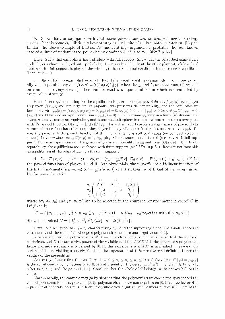
44 I. BASIC RESULTS ON NORMAL FORM GAMES
b. Show that, in any game with continuous pay-o function on compact metric strategyspaces, there is some equilibrium whose strategies are limits of undominated strategies. [In par-ticular, the above example of Bertrand's undercutting argument is probably the best knowncase of a limit of undominated points being dominated, cf. also ex. I.3Ex.7 p. 33.]
Hint. Show that each player has a strategy with full support. Show that the perturbed game where
each player's choice is played with probability 1 − ε, (independently of the other players), while a xed
strategy with full support is played otherwise , satises the usual conditions for existence of equilibria.
Then let ε→ 0.
c. Show that no example like sub I.4Ex.13a is possible with polynomials or more gener-ally with separable pay-os f(x; y) =
Pn1 gi(x)hi(y) (when the gi and hi are continuous functions
on compact strategy spaces): there cannot exist a unique equilibrium which is dominated byevery other strategy.
Hint. The requirement implies the equilibrium is pure say (x0, y0). Subtract f(x0, y) from player
I's pay-o f(x, y), and similarly for II's pay-os: this preserves the separability, and the equilibria: we
have now, with ϕy(x) = f(x, y), ϕy(x0) = 0, ϕy0(x) = 0, ϕy(x) ≥ 0, and ‖ϕy‖ > 0 for y = y0 (if ‖ϕy‖ = 0,(x0, y) would be another equilibrium, since ψx0(y) = 0). The functions ϕy vary in a nite (n)-dimensionalspace, where all norms are equivalent, and where the unit sphere is compact: construct thus a new game
with I's pay-o function G(x, y) = [ϕy(x)]/ ‖ϕy‖, for y = y0, and take for strategy space of player II theclosure of those functions (for computing player II's pay-o, points in the closure are sent to y0). Do
now the same with the pay-o function of II. The new game is still continuous (on compact strategy
spaces), but now since maxxG(x, y) = 1, ∀y, player I's minmax pay-o is > 0 (strategy with full sup-
port). Hence an equilibrium of this game assigns zero probability to x0 and to y0 (G(x0, y) = 0). By the
separability, the equilibrium can be chosen with nite support (ex. I.3Ex.10 p. 34). Reconstruct from this
an equilibrium of the original game, with same support.
d. Let F1(x; y) = y[x3 (1 + 2y)x2 + (2y + 12y2)x], F2(x; y) = F1(y; x) ((x; y) 2 [0; 1]2) be
the pay-o functions of players I and II. As polynomials, the pay-os are a bi-linear function of
the rst 3 moments (1; 2; 3) (i =
R 10 x
i(dx)) of the strategy of I, and of (1; 2; 3), givenby the pay-o matrix: 0@
1 2 3
1 0; 0 2;1 1=2; 12 1; 2 2;2 0; 03 1; 1=2 0; 0 0; 0
1Awhere (1; 2; 3) and (1; 2; 3) are to be selected in the compact convex moment space C in
R3 given by
C = f (1; 2; 3) j 22 13; (1 2)2 (1 1)(2 3)together with 0 3 1 g
Show that indeed C = fR 10 (x; x
2; x3)(dx) j 2 ([0; 1]) g.Hint. A direct proof may go by characterising by hand the supporting ane functionals, hence the
extreme rays of the cone of third degree polynomials which are non-negative on [0, 1].Alternatively, write a polynomial as At·X all vectors being column vectors, with A the vector of
coecients and X the successive powers of the variable x. Then AtXXtA is the square of a polynomial,
hence non-negative; since µ is carried by [0, 1], this remains true if XXt is multiplied by powers of xand/or of 1 − x, yielding a matrix Y . Thus the expectation of Y is positive semi-denite. Hence the
validity of the inequalities.
Conversely, observe rst that on C, we have 0 ≤ µ3 ≤ µ2 ≤ µ1 ≤ 1; and that µ ∈ C | µ22 = µ1µ3
is the set of convex combinations of (0, 0, 0) and a point on the curve (x, x2, x3) and similarly for the
other inequality and the point (1, 1, 1). Conclude that the whole of C belongs to the convex hull of the
curve.
More generally, the converse may go by showing that the polynomials we considered span indeed the
cone of polynomials non-negative on [0, 1]: polynomials who are non-negative on [0, 1] can be factored in
a product of quadratic factors which are everywhere non-negative, and of linear factors which are of the

SECT. 4 . EXERCICES 45
form (x+ a) or (a+ 1− x) for a ≥ 0. Decompose the quadratic factors as sums of two squares, and the
linear factors into the sum of the constant non-negative polynomial a (a square) and either x or 1 − x:our whole polynomial is now rewritten as a sum of products of a square with powers of x and of 1− x.
e. Show that the game dened sub I.4Ex.13d has a unique Nash equilibrium, (0; 0), whilestrategy 0 is dominated by 1, with strict inequality for all strategies of the opponent dierentfrom the equilibrium strategy.
Hint. The dominance is clear. The statement does not depend on the factor y in F (x, y). Let
ϕy(x) = F1(x, y)/y. For y > 0, ϕ′y(0) > 0, ϕ′
y(y) < 0, there is a local maximum x(y) in ]0, y[, withϕy(x(y)) > ϕy(y). Also ϕy(y) − ϕy(1) ≥ 0 thus x(y) < y is the global maximum. By symmetry,
conclude that there is no equilibrium where one player's strategy is pure and = 0. And if the pure
strategy is zero, since it is as good a reply as 1, it means the opponent also uses zero with probability
one. Thus there only remains to consider equilibria where no player uses a pure strategy. For any such
strategy of II, player I's pay-o function is of the form Ax3 + Bx2 + Cx, with A > 0, C > 0: thus
if the maximum is not unique, it is a set of the form x0, 1 with 0 < x0 < 1. Thus also II uses a
mixture on y0, 1 with probabilities q and 1 − q, with 0 < y0 < 1, 0 < q < 1: in player I's pay-owe have B = −1 − 2(qy0 + 1 − q). On the other hand, since I is indierent between x0 and 1, we haveAx3+Bx2+Cx = (x−x0)2(x−1)+ constant, hence B = −1−2x0. Thus x0 > y0 and dually y0 > x0.
f. In
x; 0 x2; x 0; 00; 1 0; 0 1; 0
player I also has to choose x 2 [0; 1] if he selects the top row.
This game also has a unique Nash equilibrium, where player I uses a dominated strategy. Further
the game is almost strictly competitive: the unique equilibrium strategies are also dominant
strategies in the game where each player would instead try to minimise his opponent's pay-o
thus we are as close to the zero-sum situation and to nite games as one could possibly get (cf.
I.4Ex.13g and I.4Ex.13h)). But the game no longer has the avour of Bertrand's undercutting,
player II's strategy is not dominated (cf. I.4Ex.13b and I.4Ex.13g), and the dominating strategy
of player I is no longer strictly better for every strategy dierent from the equilibrium strategy
(cf. I.4Ex.13i).
Remark 4.3. As dened by Aumann (1961a), almost strictly competitive means:
equilibrium pay-os in (g1; g2) and (g2;g1) are the same
the sets of equilibria in (g1; g2) and (g2;g1) intersect.Then there exists (s; t) such that s realises maxsmin g1 and minsmax g2 (and similarly for t). s isnot a dominant strategy.
g. If player I has a nite strategy set, his set of undominated mixed strategies is closed and is
a union of faces. Indeed, if is dominated, say by ~, then any convex combination +(1)(0 < < 1) is also dominated by ~ + (1 ) . Thus, in a nite dimensional vector space
ordered by an arbitrary positive cone, the set of admissible points of a compact polyhedron is a
union of faces (Cf. Arrow et al., 1953).
h. In the zero-sum situation, say under the assumptions of Theorem 2.6 p. 17, there alwaysexist undominated optimal strategies.
Hint. Under those assumptions, show that every strategy is dominated by an undominated strategy.
(Use Zorn's lemma or an equivalent).
i. If player II's strategy set is nite, player I's is compact, and the pay-o continuous, andif there is an equilibrium where I's strategy is dominated by another one which is strictly betterfor every strategy of II dierent from the equilibrium strategy, then there is another equilibrium.
Hint. Since player I maximises, the dominating strategy will then dominate a neighbourhood of his
equilibrium strategy. Apply then I.4Ex.13b, only II's strategy has to be perturbed.
14. (Dasgupta and Maskin, 1986) Let Si = [0; 1] for all i and let F be a nite family of
one-to-one continuous mappings from [0; 1] to [0; 1]. Let A(i) = f s j 9j 6= i; 9f 2 F : sj = f(si) g.Assume that F i is continuous on B(i) for all i, with B(i) A(i).

46 I. BASIC RESULTS ON NORMAL FORM GAMES
a. Dene Gn as the initial game restricted to Sin = f k=n j k = 0; 1; : : : ; n g for all i and
let n be a corresponding equilibrium such that n converges (weak) to and F i(n) converges
to some F i, i = 1; : : : ; n. Prove that there are at most countably many points si such that
F i(si; −i) > F i. (Prove rst that for such an si one has −i(f s−i j (si; s−i) 2 Ai g) > 0 and that
this implies: 9j 6= i, 9f 2 F , j(f(si)) > 0).
b. Assume moreoverPn
i=1Fi u.s.c. and that each F i satises, for all si 2 Bi(i):
9 2 [0; 1] such that for all s−i with s = (si; s−i) 2 B(i), lim inftisiFi(ti; s−i) + (1
) lim inftisiFi(ti; s−i) F i(s). Prove that is an equilibrium with pay-o F .
c. Extend the result to Si compact convex in some Rm.
d. Consider the two-person symmetric game with
F 1(s1; s2) =
(0; if s1 = s2 = 1;
s1; otherwise.
(Note that F 1+ F 2 is not u.s.c. at (1; 1)).
15. Fictitious Play. (Robinson, 1951) Fictitious play is the procedure where each player
chooses at every stage a best reply against the distribution of his opponent's past choices. We
prove here that, for zero-sum games, the frequency of moves converges to the optimal strategies.
Given an m n real pay-o matrix A, write Ai for the row i and Aj for the column. Call
admissible a sequence ((t); (t)) in RnRm, t 2 N satisfying:
(1) infj j(0) = supii(0).(2) 8t 2 N;9i : (t+ 1) = (t) +Ai, with i(t) = supk k(t).(3) 8t 2 N;9j : (t+ 1) = (t) +Aj, with j(t) = infkk(t).
Say that i (resp. j) is useful in (t1; t2) if there exists t in N with t1 t t2 and i(t) = supk k(t)(resp. j(t) = infkk(t)).
a. Prove that if all j are useful in (s; s+ t) then:
supjj(s+ t) inf
jj(s+ t) 2t kAk :
Dening (t) as supii(t) infj j(t), prove that if all i and j are useful in (s; s+ t), then:
(s+ t) 4t kAk :b. Prove by induction that for every matrix A and " > 0, there exists s in N such that
(t) "t for all t s and all admissible sequences.
Hint. Let r be such that µ′(t) ≤ εt for all t ≥ r and all admissible sequences associated to a
(strict) submatrix A′ of A with corresponding µ′. Prove that if i is not useful in (s, s + r) one hasµ(s+ r) ≤ µ(s) + εr. Finally given t = qr + s with s < r, let p be the largest integer ≤ q such that all
i, j are useful in ((p− 1)r+ s, pr+ s), and 0 if this never occurs. Show that µ(t) ≤ µ(pr+ s) + ε(q − p)rand conclude.
c. Prove that for all admissible sequences:
limt→∞(supi
i(t)=t) = limt→∞(infj
j(t)=t) = v(A)
(where v(A) is the value of A).
16. (Shapley, 1964) Consider ctitious play in the following two-person game: S1 = S2 =f1; 2; 3g
F1 =
0@a1 c2 b3b1 a2 c3c1 b2 a3
1A F2 =
0@1 1 12 2 2 3 3 3
1Awith ai > bi > ci and i > i > i for all i.

SECT. 4 . EXERCICES 47
a. Assume the rst choice is (1; 1). Prove that after a sequence of (1; 1) a sequence of (1; 3)will occur followed by a sequence of (3; 3) then of (3; 2); (2; 2); (2; 1) and (1; 1) again.
b. Denote by r11 the length of a sequence of (1; 1) and by r13 the length of the following
sequence of (1; 3). Show that r13 r11(a1 c1)=(a3 b3) and deduce inductively, if r′11 is thelength of the next sequence of f1; 1g that:
r′11 Y
i
ai ci
ai bi
i i
i i
r11:
c. Deduce that the empirical strategies do not converge. Furthermore, no subsequence
converges to the (unique) equilibrium pair.
17. On xed points. Note that the quasi-concavity assumption in theorem 4.1 p. 39 was
not used in its full force only the convexity of the best reply sets was used. But even this is
too much: given an upper semi-continuous correspondence T from a compact convex set S to
itself, the condition for T to have a xed point should be purely topological. This is the aim of
the present exercise. In fact, it will be more convenient to argue in terms of a compact Hausdor
space X (e.g. the graph of T ), together with two (continuous) maps f and g from X to S (e.g.,
the two projections). We look then for a solution of f(x) = g(x), and the best reply sets are the
sets f−1(s).We assume also that S is Hausdor, that f is onto and that ~Hq(f−1(s)) = 0 for all q 0
and s 2 S, where ~H denotes reduced ech-cohomology with coecients in a module G (Spanier,
1966). We express this condition shortly by saying that f is (G)-acyclic, this is a purely topolo-
gical condition on the best reply sets, satised as soon as each of them is contractible (homotopy
invariance). Similarly we call an upper semi-continuous correspondence from X to S acyclic
if the projection from its graph to X is so, i.e., if 8x 2 X, ~Hq((x)) = 0 and (x) 6= ;.a. Prove that, when S is a nite dimensional convex set, there exists a solution (of
f(x) = g(x)).
Hint. Denote by ∂S the boundary of S, and let ∂X = f−1(∂S). Apply the Vietoris-Begle mapping
theorem (Spanier, 1966, VI.9.15) to f : X → S and to f : ∂X → ∂S to conclude by the ve lemma
(Spanier, 1966, IV.5.11) and exactness (Spanier, 1966, V.4.13) that f : (X, ∂X) → (S, ∂S) is an iso-
morphism in ech-cohomology. If f(x) = g(x) for all x, construct (as in Spanier, 1966, IV.7.5) a map
f : X → ∂S which is homotopic to f . Conclude to a contradiction.
b. To show that acyclic maps are the right class of maps for this problem, prove that iff : X ! Y and g : Y ! Z (all spaces compact) are (G)-acyclic, so is g Æ f .
Hint. Clearly g f is onto. Let S = g−1(z) : Hq(S) = 0. Since f as a map from X = f−1(S) to Sis acyclic, f∗ : Hq(S) → Hq(X) is an isomorphism (cf. a)): Hq(X) = 0 for all sets X = (g f)−1(z).
c. A continuous ane map f on a compact convex subset X of a Hausdor topologicalvector space is acyclic to f(X).
Hint. Use the above mentioned contractibility criterion.
d. Assume S is a compact convex subset of a topological vector space, such that points ofS are separated by continuous ane functionals on S shortly henceforth: a compact convexset. Prove that there exists a solution.
Hint. By the separation property on S and compactness of X it suces to show that (p f)(x) =(p g)(x) has a solution for every continuous ane map p : S → Rk. Use I.4Ex.17b and I.4Ex.17c to
show that p f and p g satisfy the conditions sub I.4Ex.17a.

48 I. BASIC RESULTS ON NORMAL FORM GAMES
e. If S is a retract of a compact convex set Y , there exists a solution.
Hint. The assumption means that there are continuous maps i : S → Y and r : Y → S such that
(r i)(s) = s, ∀s ∈ S. Let then X = (x, y) ∈ X × Y | f(x) = r(y) ; denote by p1 and p2 the two
projections, and apply I.4Ex.17d to f = p2 and g = i g p1.At this stage we have a purely topological statement. To see that those are the right assump-
tions, note that the statement remains true, but without additional generality, if g is replaced
by an acyclic correspondence from X to S. Slightly more generally, since f−1 is an acyclic
correspondence from S to X, we have:f. Let Xi (i = 0; : : : ; n) be compact Hausdor spaces, with X0 = Xn being a retract of a
compact convex set. Let i(i = 1; : : : ; n) be (G)-acyclic correspondences from Xi−1 to Xi. Thentheir composition has a xed point x 2 (x). [(1 Æ 2)(x0) =
Sx1∈Γ1(x0)
2(x1)].
Hint. Let Yj = (x0, . . . , xj) ∈∏i≤jXj | xi ∈ Γi(xi−1) for 0 < i ≤ j , with projection fj to Yj−1.
Then the fj are acyclic, hence I.4Ex.17b so is their composition f : Yn → X0. Let also g : Yn → Xn(= X0)denote the projection to the last coordinate, and apply I.4Ex.17e.
This proof shows, in other words, that the class of correspondences which are the composition
of a (G)-acyclic correspondence with a continuous map is stable under composition.
g. Reverting to our context of games, use Künneth's formula (Spanier, 1966, VI.Ex.E) to
show that, if G is a eld, the best reply correspondence will be acyclic if and only if any best
reply set B of any single player satises ~Hq(B) = 0.
Comment 4.4. The above appears as the correct formulation for this type of xed point
theorem. Nevertheless, one sees that the crux of the problem lies in the case where S is an
n-dimensional compact convex set; and there the assumption on f is only used to ensure that
the map f∗ from ~Hn(S; @S) to ~Hn(X; @X) is non-zero (and hence that f is not homotopic to a
map to @S). This assumption is much too stringent for that, and other much more exible tools
are available to prove such things (e.g., homotopy invariance of f∗). But for proving existence
of (pure strategy) Nash equilibria, this is already a reasonably good tool.
18. Knaster-Kuratowski-Mazurkiewicz Theorem. Consider the n-simplex with itsfaces Fi = fx 2 j xi = 0 g (i = 0; : : : ; n). Let Ci be closed subsets, with Fi Ci,
SiCi = .
ThenT
iCi 6= ;.Hint. Let fi(x) = d(x,Ci), f(x) =
∑n0 fi(x), ϕ(x) = (fi(x)/f(x))ni=0 : ϕ is a continuous map from
∆ to ∂∆, with ϕ(Fi) ⊆ Fi. View now ∆ as the unit ball: the map x→ −ϕ(x) is a continuous map from
∆ to itself without xed point. Apply ex. I.4Ex.17
Comment 4.5. Observe that the last part of the proof also shows that the sphere is not a
retract of a compact convex set (otherwise x! x contradicts ex. I.4Ex.17).
19. Deduce lemma 1.7 p. 5 from I.4Ex.18.
Hint. Select the extreme point ei of ∆ in⋂j =iTj.
20. Also the continuity assumption in theorem 4.1 p. 39 was not the right one even in
the more general framework of ex. I.4Ex.17: it is sucient to assume for each player i that hispay-o function F i is upper semi-continuous on
Qj S
j, and is, for each xed si 2 Si, continuous
in the other variables jointly and, if one wants a mixed strategy version, like theorem 4.1, and
not a pure strategy version like ex. I.4Ex.17, to assume furthermore that F i is bounded and the
Si strictly semi-compact (ex. I.1Ex.7c p. 12), or F i continuous in si using ex. I.2Ex.1c p. 21.
Hint. Write shortly S for Si, T for∏j =iS
j, F : S × T → R for F i. Let R = (s, t) | F (s, t) =maxs∈S F (s, t) . Show that R is closed under the above assumptions. This yields the pure strategy
version of ex. I.4Ex.17. For the mixed strategy version, upper semi-continuity and boundedness imply
that the mixed extension is well dened. Use then the stated exercises.

SECT. 4 . EXERCICES 49
21. Teams. A team problem (game with nite strategy spaces where all players have thesame pay-o function) has nitely many equilibrium pay-os.
Hint. It suces to show that there are nitely many pay-os to completely mixed equilibria. Show
that, at such an equilibrium, the gradient of the pay-o function is zero, and use Sard's theorem (e.g.
Milnor, 1969, p. 16) to deduce that the set of completely mixed equilibrium pay-os has Lebesgue measure
zero. The semi-algebraicity of this set (cor. 3.4 p. 27) implies it is a nite union of intervals.
22. Games with pay-o correspondence. (Simon and Zame, 1990) Consider an Nperson game with strategy spaces Si and a correspondence Q from S to RN . Assume each Si
compact Hausdor, Q non-empty compact convex valued and u.s.c. (3). Prove the existence of
a Borel selection q of Q such that the game (Si; i = 1; : : : ; N ; q) has an equilibrium.
Hint. For any nite game (Siα nite and included in Si and qα an arbitrary selection of the graph
of Q above Sα) choose equilibrium strategies µα = (µiα). Let µα and qαdµα converge weakly (along some
ultralter rening the increasing net of all nite subsets Siα) to µ and ν and note that ν is absolutely
continuous w.r.t. µ. Let q be µ-measurable with qdµ = dν. Then µ s | q(s) /∈ Q(s) = 0; otherwisechoose a, b ∈ Q and x ∈ QN such that V = s | 〈q(s), x〉 > a > b > 〈t, x〉, ∀t ∈ Q(s) has positive
measure. Use then the regularity of µ and Urysohn's lemma to get a contradiction. Change q on a set
of µ measure 0 to get a Borel selection and let us still write q for the mixed extension. Show (as above)
that T i = si ∈ Si | qi(si, µ−i) > qi(µ) has µi measure 0. To get an equilibrium we nally modify q asfollows: let p[i] be a selection of Q minimising i's pay-o and dene
q(s) =
p[i](s), if si ∈ T i, sj /∈ T j, j = i;q(s), otherwise.
Note that qi(µ) = qi(µ) and qi(·, µ−i) = qi(·, µ−i) on Si\T i. Finally on T i, since Q u.s.c. implies p[i]i l.s.c.one has: qi(ti, µ−i) = p[i]i(ti, µ−i) ≤ lim infα p[i]i(tiα, µ−iα ) ≤ lim infα q
iα(tiα, µ−iα ) ≤ lim infα q
iα(µα) ≤ qi(µ).


CHAPTER II
Basic Results on Extensive Form Games
1. The Extensive Form
The extensive form is the most commonly used way to describe or to dene a game.
We give here a rather general description with some typical variants. The aim is among
others to have nite extensive forms, e.g. for repeated games (cf. comment 1.3 below), so
as to be able to dene them eectively in this way. The exibility is also needed to de-
scribe the solutions of some repeated games with incomplete information as the solutions
of auxiliary nite games (ch.VIII, sect. 2 p. 361; also ex.VIIIEx.2 p. 393).
1.a. Denitions.
Definition 1.1. An extensive form game consists of
(1) a player set I = f1, . . . , Ig;(2) a space of positions Ω;(3) a signal space A and a function α from Ω to (probabilities on) A;(4) a partition (Ai)i∈I of A;(5) an action space S and a function q from ΩA S to (probabilities on) Ω;(6) for each i, a pay-o function gi from Ω∞
to R;
(7) an initial position ω1.
Of course, when dealing with probabilities sub 3 and 5, appropriate precautions will
have to be taken, cf. 1.c below. Also when there are no probabilities, the factor A in 5 is
redundant.
Each player i 2 I has to decide what action s 2 S to choose when he is told a in Ai,
i.e. to dene a function σifrom Ai
to S. The game is then played as follows: at stage n,an will be chosen according to α(ωn), and if it belongs to Ain, the next position ωn+1 will
be chosen according to q(ωn, an, σin(an)). In other words, if an belongs to A
i, player i has
the move: in that case, he is told the signal or message an and nothing else: he does not
remember his past information or his past choices and not even the stage n itself, if they
are not explicitly included in the message. He selects then an action sn as a function of
this signal and the new position ωn+1 is selected using q(ωn, an, sn). Each player i receivesat the end of the game the pay-o gi(ω1, ω2, . . . ). In some sense, each player i decidesat the beginning of the game on σi
the program of his machine and the game
then proceeds purely automatically. σiis called player i's pure strategy. Signals (in the
deterministic case) are often identied with their inverse images in the set of positions
called information sets.
Some variants.
(1) When ω1 is chosen at random, add an additional initial state ω0, and extend qand α appropriately.
(2) Often a set of terminal positions is needed, where the game stops. This can
be formalised by leaving those positions xed under q, whatever be the action s
51

52 II. BASIC RESULTS ON EXTENSIVE FORM GAMES
in S. Conversely, if after a position only one sequence of positions is possible, we
can replace it by a terminal position.
(3) Usually, for any signal a in A, only a (non-empty) subset of actions in S is
allowed. This can be taken care of either by allowing in the denition for an
S-valued correspondence on A and then dening q only on the relevant set
or by keeping the above denition and extending q and g outside this set in a
proper way say by duplication: any additional move is equivalent to some xed
strategy. But the second trick cannot be used when discussing perfect recall and
behavioural strategies (cf. below): indeed, if one does not inform the player of
which duplicate was used, one looses the perfect recall property, and if one does,
one introduces in the new game additional behavioural strategies, which are not
behavioural strategies of the original game, but mixed (or general) strategies
(cf. below for the terminology). Hence in those cases we will write S for the
S-valued correspondence on A, i.e., its graph in A S (thus: Sa for its value at
a). q is then dened on Ω S.(4) Another formulation that leads to deterministic signals: take Ω∗ = Ω A and
dene q∗ from Ω∗ S to probabilities on Ω∗using rst q and then α. α∗
is
then the deterministic projection from Ω∗to A, or simply a sub σ-eld C on Ω∗
.
The partition (Ai)i∈I becomes then a C -measurable partition Ω∗i of Ω∗
, and σiC -measurable on Ω∗
i .
Let Ω′ = Ω A S (or Ω S in case of variable action sets), and denote by Ω′n the
nth copy of Ω′. Let H∞ =
Q∞1 Ω
′n be the set of plays, while the set H of histories is the
set of (nite, possibly empty) initial segments of plays.
Remark 1.1. There is no need to allow, like sub 3, for position-dependent sets of
possible signals, or similarly for variable sets of possible new positions. Indeed, the trans-
ition probabilities q and α describe already in some sense what is possible, so one would
add a new primitive concept which duplicates to a large extent the information already
available in the model. Further, here there is no problem in using the full containing space
A (or Ω), extending the transition probability q in an arbitrary way when its arguments
are not feasible.
The only drawback is that we will in general not have a meaningful denition of a
set of feasible plays, since it will depend on this containing space A. The set can be
dened meaningfully only when all probabilities in the model are purely atomic: then one
should dene the set as consisting of those plays such that each of their initial segments
has positive probability under some strategy vector. Hence, in the general denition below
of linear games and of (eectively) perfect recall, we will have to avoid using this concept
of feasible play.
1.b. Finite case. Here we consider games where there are nitely many dierent
(feasible) plays. As dened above, a pure strategy for i is a mapping from Aito S. A
mixed strategy will be a probability distribution on those. A behavioural strategyis
a mapping from Aito probability distributions on S. Finally, a general strategywill be
a probability distribution on the (compact) set of behavioural strategies. (For the solution
of such games, cf. ex. II.1Ex.3 p. 57).
An I-tuple of (general) strategies denes a probability distribution on plays. Two stra-
tegies of a player are equivalent if they induce the same distribution on plays whatever
be the strategies of the other players. The normal form of the game associates to

1. THE EXTENSIVE FORM 53
every strategy vector the corresponding vector of expected pay-os (normal form in pure
strategies, in mixed , in behavioural , in general ).
The above denition of the extensive form does not exclude that a play may produce
twice the same message. There could even be two identical positions at two dierent
stages along the same play. We call the game linear (Isbell, 1957) (for player i) if, a.e. forevery strategy vector, every message of player i occurs at most once along every play. (All
the games that we will study in this book will be linear; however, some nite, non-linear
games will occur as auxiliary games to solve a class of repeated games with incomplete
information (cf. ch. VIII). The term linear is related to the following property:
Theorem 1.2. (Isbell, 1957)In a linear game (for player i), every general strategyof i is equivalent to a mixed strategy.
Proof. In fact, given a behavioural strategy τ of player i, we will construct a mixed
strategy inducing the same probability on plays, whatever be the other players' strategies.
Let µ be dened on each pure strategy σ by:
µ(σ) = Prµ(σ) =Y
ai∈Aiτ(ai)fσ(ai)g .
It is then clear that, given any strategies of the other players, the probability of the cor-
responding sequence of moves in S will be the same under τ and µ. Obviously, the same
result holds for general strategies, taking the expectation w.r.t. to τ .
To see the need for the assumption linear, cf. ex. II.1Ex.2 p. 56. For a more general
case, cf. ex. II.1Ex.10d and II.1Ex.10e p. 63.
The game is said to have (eectively) perfect recall for player i if (knowing the purestrategy he is using), he can deduce from any signal he may get along some feasible play,
the sequence of previous messages he got along that play. (All the games we will study
will have eectively perfect recall). Observe that a game with eectively perfect recall for
i is necessarily linear for i. In other words, for having perfect recall, every message must
in particular recall both the last message and the last action, while, for having eectively
perfect recall, it is sucient that the player be able to reconstruct the last message, in
that case, he can also, knowing his pure strategy, reconstruct his last action, and so on:
this shows inductively that he can do as well as if he remembered also his past actions.
Formally we have:
Theorem 1.3. (Dalkey, 1953) In a game with eectively perfect recall for player i,his pure strategy set is essentially the same (i.e. except for duplication) whether or nothe recalls, in addition to his current information, his own past signals and moves.
Proof. A pure strategy of player i when he recalls his own past signals and choices
is of the form: fsn = σ(a1, . . . , an; s1, . . . , sn−1)g for n 1, where (a1, . . . , an) denotes thesequence of signals from Ai
he has heard, (s1, . . . , sn−1) is the sequence of his past choicesin Si
and sn in Siis the move to be chosen. Dene, by induction on the number n of
signals previously heard, a strategy φ that depends only on the current signal: roughly, foreach initial signal a in Ai
, s1 = φ(a) = σ(a). Inductively, given a signal a, deduce from aand φ the previous signals, say a1, . . . , an, and let φ(a) = σ(a1, . . . , an, a;φ(a1), . . . , φ(an)).Whatever be the strategy of the other players, the pure strategy φ results in the same
probability distribution on plays as the pure strategy σ, hence the proof is complete.
For more details and/or more generality, cf. ex. II.1Ex.14 p. 72.

54 II. BASIC RESULTS ON EXTENSIVE FORM GAMES
Comment 1.2. Observe that, since the set of strategies φ is clearly smaller than the
set of strategies σ by our construction, several strategies σ will be mapped to the same
strategy φ. This is the duplication of strategies mentioned above.
Comment 1.3. From our previous denitions, it appears that, for a game with eect-
ively perfect recall, we need a very large space of positions, essentially H. But it follows
from the above that, to specify a game with eectively perfect recall, it is sucient to
describe each player's incremental information every time he has to play. This can be
arbitrary, in particular does not have to remind him his last move. This is the way we
will describe all our models in this book from ch. IV on: the signal a 2 Aiwill be player i's
incremental information. (I.e., his true signals, in the previous general model, are nite
sequences in Ai.) Therefore we will still be able to use small (nite) sets of positions.
The main advantage of games with perfect recall is the following.
Theorem 1.4. (Kuhn, 1953) In a game with perfect recall for player i, general,mixed, and behavioural strategies are equivalent for i.
Proof. By theorem 1.2 p. 53, it is enough to represent any mixed strategy µ by a
behavioural strategy τ . In fact, given µ, probability distribution on pure strategies, com-
pute rst, for every initial signal a1 (cf. ex. II.1Ex.8 p. 59), the marginal distribution µa1
on strategies after a1, compute then from µa1the marginal distribution τa1
of s1, and the
conditional distribution µa1,s1 on strategies for the future given s1. Continue then with
µa1,s1 as before with µ.
As a corollary, by Dalkey's theorem, one can also study games with eectively perfect
recall by using behavioural strategies in the corresponding game with perfect recall.
A game is said to have perfect information if the position at each stage in a feasible
play determines all the previous positions along the play and moreover the signal determ-
ines the position. In other words, when he has to play, each player knows the whole past
history.
Theorem 1.5. (Zermelo, 1913) In a game with perfect information, there exists anequilibrium in pure strategies.
Proof. The proof is very simple using backwards induction: Replace each posi-
tion that is followed only by terminal positions, by a terminal position with, as pay-o,
the pay-o corresponding to an optimal choice of action of the player having the move at
that position.
1.c. A measurable set up. We consider now a game where the spaces Ω, A and
S are measurable as well as the partition (Ai)i∈I, the graph S and the map g; α and qare transition probabilities. A pure strategy, say for player i, is then a measurable se-
lection from S dened on (Ai,A i). Similarly, a behavioural strategy will be a transition
probability from (Ai,A i) to (S,S ), assigning probability one to S. Note that there is
no adequate measurable structure on those sets, hence it is more appropriate to dene a
mixed strategy as a measurable selection from S dened on (X i Ai, X i A i) where
(X i,X i, Qi) is an auxiliary probability space. One similarly denes general strategies as
transition probabilities from (X i Ai, X i A i) to (S,S ) assigning probability one to
S.
Proposition 1.6. An I-tuple of general strategies induces a unique probability dis-tribution on plays.

1. THE EXTENSIVE FORM 55
Proof. Use Ionescu Tulcea's theorem (Neveu, 1970, prop.V.1.1) with (ΩAS)∞,then show that (Ω S)∞ has probability one.
Hence, the normal form will be well dened (so one can speak of equilibria) e.g.
as soon as g is bounded from below or from above. And, since for each x 2Q
iXi
we also have a vector of strategies, the corresponding pay-o g(x1, x2, . . . ) is also well
dened, and, by the cited theorem, it will be a measurable function onQ
iXi, with
g(Q1, Q2, . . . ) =Rg(x1, x2, . . . )
Qi∈I dQ
i.
It also follows that the denition of the equivalence of strategies extends to this case.
In particular, if general strategies are shown to be equivalent to mixed strategies (cf.
ex. II.1Ex.10d p. 63) a strategy vector is an equilibrium i no player has a protable pure
strategy deviation.
Definition 1.7. A game has (eectively) perfect recall for player i if, (for everypure strategy of i), there exists a measurable map ϕ from Ai
to (AiSi)[ fιg such that,
for every strategy vector of i's opponents a.s.: ϕ(a) = ι means that a is the rst signal tothis player, otherwise ϕ(a) is the previous signal to him and the action he took upon it.
(For a justication of this denition, cf. ex. II.1Ex.12 p. 64).
Theorem 1.8. Assume player i has perfect recall and (S,S ) is standard Borel (cf.App.6). Every general strategy of player i is equivalent to a mixed strategy and to abehavioural strategy.
Proof. To prove the inclusion of general strategies in the set of mixed strategies,
represent (S,S ) as [0, 1] with the Borel sets; then a general strategy yields a family of cu-
mulative distribution functions Fx,a(s) jointly measurable in x, a and s (ex. 1 p. 61). Theperfect recall assumption implies there is a measurable map n(a) (ex. II.1Ex.10 p. 61) fromAi to N that increases strictly along every play. Let then un be an independent sequence
of uniform random variables on [0, 1], and dene µ(u, x, a) = minf s j Fx,a(s) un(a) g: µ isa mixed strategy with as auxiliary space the product (X i,X i, Qi) ([0, 1],B, λ)N, whereλ denotes Lebesgue measure on the Borel sets B of [0, 1]. And Pr(µ s j x, a, past)= Pr(un(a) Fx,a(s) j x, a, past) = Fx,a(s), so µ induces clearly the same probability
distribution on plays as the general strategy.
The proof of the second part is given in ex. II.1Ex.10 p. 61.
Actually, the above is the proof of a dierent statement, cf. ex. II.1Ex.10d.
Ex. II.1Ex.10a and II.1Ex.10b give a full proof of theorem 1.8; part II.1Ex.10a being
there only to justify the clearly in the last sentence of the proof above.
Comment 1.4. When Aiis countable (cf. also ex. II.1Ex.14, comment 1.28 p. 73), a
behavioural strategy can be identied with a point in [S∗]Ai, denoting by S∗the set of
probability distributions on S. The σ-eld S induces a natural σ-eld on S∗(requir-
ing that the probability of every measurable set be a measurable function on S∗), and
hence on [S∗]Ai
. Thus general (resp. mixed) strategies are naturally dened as probability
distributions on [S∗]Ai
, resp. SAi
. Those denitions are clearly equivalent to the former
(without any standard Borel restrictions): given a probability distribution P on [S∗]Ai
, use
([S∗]Ai
, [S ∗]Ai
, P ) as (X i,X i, Qi) this also reduces to the former case how to dene the
probability distributions induced on plays by those new strategies ; conversely, given
(X i,X i, Qi) there is an obvious measurable map to ([S∗]Ai
, [S ∗]Ai
) dening a P (and si-
milarly for mixed strategies). It is clear that this transformation preserves the probability

56 II. BASIC RESULTS ON EXTENSIVE FORM GAMES
distribution induced on plays. This probability distribution is clearly the average under Pof the distributions induced by the underlying behavioural (resp. pure) strategies. Thus
we are led back at least for linear games (cf. ex. II.1Ex.10c p. 63) to the general
concept (ch. I) of a mixed strategy as a probability distribution over pure strategies, and
the corresponding normal forms.
Comment 1.5. When A is countable, and topologies on Ω and S (often: discrete
topologies) are given for which q and α are continuous, the induced mapping from pure
strategies (SAwith the product topology) to plays (product topology) will be continu-
ous too, so that continuity properties of g translate immediately into the same (joint)
continuity properties of the normal form pay-o function (and compactness of S yields
compactness of SA).
Exercises.
1.
a. Show that a game as dened in 1.a p. 51 can also be represented by a deterministic one
i.e. and q functions by adding nature as player zero (which uses a xed behavioural
strategy).
Comment 1.6. This modication is frequently useful in specic situations, because it allows
to have a smaller and more manageable set of (feasible) plays, by giving variable actions sets to
nature as well as to the other players.
b. Observe that, in such a game with moves of nature, one can always redraw the tree such
that the game starts with a move of nature, and is deterministic afterwards, i.e. the only ran-
domness is in the selection of the initial position. (Use theorem 1.4 p. 54 or its generalisation
sub ex. II.1Ex.10 p. 61 below for player zero, getting a mixed strategy for him.)
c. Similarly, one can also redraw the tree such as to let nature postpone as much as pos-
sible its choices (thus histories of the form (a1; s1; a2; s2; a3; s3; : : : )), by obtaining this time a
behavioural strategy for player zero.
Comment 1.7. This transformation is often important: e.g. in ch.VIII, it will reduce a class
of games with symmetric information to stochastic games.
2. (Isbell, 1957) In the two-person zero-sum game of Figure 1, show that:
root
b
b
b
b
b
0 0
1
1
1 1
0 0 0
I II I
Figure 1. A non-linear Game
by randomising (1=2; 1=2) between (3=4; 0; 1=4; 0; 1) and (0; 3=4; 1=4; 1; 0) player I canguarantee 9=16.

SECT. 1 . EXERCICES 57
he cannot guarantee more than 1=2 with mixed strategies.
he cannot guarantee more than 25=64 with behavioural strategies.
3. Polynomial pay-o functions.
a. Prove that, in a game with nitely many dierent feasible plays, the pay-o is polynomial
in behavioural strategies.
b. Show that any polynomial pay-o function on a product of compact, convex strategypolyhedra can be obtained in this way.
Hint. Reduce rst to the case of strategy simplices. Show then how to construct a sum, and reduce
thus the problem to the case of the same pay-o function to all players, which is a single monomial.
See ex. I.4Ex.8 p. 41 to show that such games have nite solutions.
4. An n-dimensional moment problem.a. Let P (x) be a polynomial, with P (x) > 0 for x > 0. Show that, for n suciently large,
all coecients of (1 + x)nP (x) are positive.
Hint. The binomial formula yields the n-step distribution of a random walk. Use the corresponding
asymptotic approximations. In a more elementary fashion, factor rst P into linear and quadratic factors
of the form x+ q and (x− p)2+ q, with q > 0, so as to reduce the problem to P (x) = (x− p)2+ q, p > 0,q > 0, which can then be handled in a fully elementary way, remaining within the realm of second degree
equations.
b. Let P (x1; y1;x2; y2; : : : ) be a polynomial, homogeneous in each pair (xi; yi)(1 i k).Assume P > 0 whenever xi 0; yi 0, xi + yi > 0 for all i. Show that, for n suciently large,all coecients of [
Qi(xi + yi)
n]P (x; y) are positive.
Hint. Induction on k. For xed values xi ≥ 0, yi ≥ 0 for i ≥ 2 (xi + yi > 0), apply II.1Ex.4a
to the resulting polynomial in x1/y1. By continuity of the coecients, they will still be positive in the
neighbourhood of z = (xi, yi) | i ≥ 2 ; use compactness.c. Let the polynomial P be positive on k = fx 2 Rk+1
+ j Pxi = 1 g. Then there is ahomogeneous polynomial T of degree d, where every possible monomial of degree d has a positivecoecient, and with P (x) = T (x) for x 2 k. If P is homogeneous, then T = [
Pixi]
nP .
Hint. Make rst P homogeneous by multiplying each monomial by the appropriate power of∑xi;
add then ε[1 −∑ixi] for ε > 0 suciently small (compactness), such as to have P (x) > 0 on the unit
cube. Obtain now Q(x, y) by replacing in P (x) every xhi by xhi (xi+yi)
di−h, where di is the maximal powerof xi in P : for x ∈ ∆k, yi =
∑j =ixj, Q(x, y) still equals the original P (x). Apply II.1Ex.4b to Q(x, y),
and let R(x, y) = [∏i(xi+ yi)n]Q(x, y): we still have R = P on ∆k, and all terms of R are non-negative,
hence this remains so when replacing all yi by∑j =ixj and expanding to obtain T (x), which is clearly
homogeneous, say of degree d. And the coecients of xdi are necessarily strictly positive. So if some othercoecients are still zero, multiplying T by an appropriate power [(k − 1)d] of
∑xi will make them all
positive. For the last sentence, set n equal to the dierence in degrees: the two polynomials are then
equal on Rk+1+ , hence are identical.
d. Let K be a compact convex polyhedron in Rn (cf. ex. I.3Ex.4 p. 29) dened by the in-equalities fi(x) 0 (i = 1; : : : ; k), where the fi are ane functionals. Any positive polynomialfunction P on K can be written as a sum with positive coecients of all monomials of somedegree d in f1; : : : ; fk.
Hint. If K is a singleton, take d = 0. Since K is compact, the fi separate points. Let
f = (fi)ki=1 : Rn → Rk: f(K) is the intersection of Rk+ with an ane subspace, say with equations
ϕi(y) = 0 (i = 0, . . . , h). The ϕi are not all linear, otherwise f(K) would be unbounded. Assume thus
ϕ0(y) = 0 is of the form∑µiyi = 1. Using this, one can make all other ϕi (i = 1, . . . , /) linear. Com-
pactness of f(K) implies it can be separated from∑yi ≥ M , which implies (e.g. ex. I.3Ex.1 p. 28) that
adding some linear combination of the ϕj (j ≥ 1) to ϕ0, one can assume µi > 0, i = 1, . . . , k. Since thefi separate points, P can be rewritten as a polynomial Q in the fi(x): Q is a polynomial on Rk, > 0 on

58 II. BASIC RESULTS ON EXTENSIVE FORM GAMES
f(K). Adding a polynomial L∑i≥1[ϕi(y)]
2 for L suciently large will not aect the values on f(K), butwill make Q > 0 on y ∈ Rk+ |∑µiyi = 1 . Apply now II.1Ex.4c.
e. Same statement as sub II.1Ex.4d, but if K is a product of compact polyhedra Kj, onecan use a sum with positive coecients of all monomials which are separately for each j of degree
dj in the fji .
Hint. Remember from the proof of II.1Ex.4d that for each Kj (#Kj > 1) we have a relation∑iµjifji = 1 with µji > 0. Make sure that indeed all possible monomials have strictly positive coecient.
Comment 1.8. Observe those results remain true in some sense for arbitrary nite dimen-
sional compact convex sets: the polynomial function is still strictly positive in some neighbour-
hood, squeeze a compact convex polyhedron (or a product) in this neighbourhood, containing the
given compact set in its interior. One obtains thus a similar representation, with a nite number
of ane functionals which are strictly positive on the given compact convex set. Hence it also
extends to compact convex sets in topological vector spaces, dening the polynomial functions
as the algebra generated by the continuous ane functionals. In particular, if C is a compact
convex set in a Hausdor locally convex space E, then any linear functional on the polynomial
functions on E which is non-negative on all nite products of continuous ane functionals which
are positive on C, is a non-negative Radon measure on C. [! A little additional exercise has to
be made, for E = Rn, to be sure to prove the result for polynomial functions on E and not just
on C.]
Comment 1.9. It would be interesting to know, even for applications like sub II.1Ex.6 be-
low, what polynomial functions have such a representation when asking only for non-negative
coecients.
5. Rational pay-o functions. Consider a nite game i.e. , A and S are nite
with a privileged position !0, from where play remains in !0. Assume that any pure strategy
vector, and starting from any position, has a positive probability of eventually reaching !0.a. Prove that the expected time for reaching !0 is uniformly bounded, over all behavioural
(hence also general) strategies (and all possible starting points).
Hint. By niteness, there exists ε > 0, and n0 < ∞ such that for any pure strategy vector, and
any starting point, ω0 is reached before n0 with probability > ε. Consider a behavioural strategy vec-
tor: by niteness of the action space S, there is for each a ∈ A an action with probability ≥ (#S)−1.
The probability that the corresponding pure strategy vector be played for the rst n0 stages is therefore
≥ (#S)−n0. Thus the probability of reaching ω0 in that time is ≥ ε(#S)−n0 = δ > 0, whatever be thestarting point and the behavioural strategy vector.
b. Assume a pay-o function is given over , zero at !0, and that the pay-o of the gameon ∞ is obtained as the sum of the stage pay-os. Prove that the pay-o is a rational functionof the behavioural strategies, with a denominator that vanishes nowhere.
Hint. Denote by P the transition probability of the resulting Markov chain on Ω, by u(ω) the
pay-o function on Ω, and let Vω denote the expected pay-o starting from ω. Then V = u + PV(u, V column vectors). The equation and the column of P corresponding to ω0 can be deleted, since
u(ω0) = V (ω0) = Pω0(ω0) = 0. II.1Ex.5a implies then that the series∑Pn is summable, so I −P has
non-zero determinant.
6. Rational pay-o functions. The converse. Conversely, show that any normal form
game, where each player i has a product of compact convex polyhedra (Kia)a∈Ai as pure strategy
space, and where the pay-o function F is rational with non-vanishing denominator, arises from
some game as sub II.1Ex.5, where Ai is the set of i's signals, where his available actions at a 2 Ai
are the extreme points v of Kia, and where the pay-o to any behavioural strategy vector
i,av
(i,av 0,
Pv
i,av = 1) is given by F [(
Pv
i,av v)a∈Ai,i∈I].

SECT. 1 . EXERCICES 59
Hint. Assume w.l.o.g. that #Kia > 1 for all (i, a), and that the corresponding set of ane con-
straints f i,ac (x) ≥ 0 satises multiplying each of them by the corresponding µc (cf. II.1Ex.4d) , that∑c fi,ac (x) = 1 identically. Denote by Ci,a the set of constraints f i,ac of Ki,a, and by V i,a its set of extreme
points.
Use a common denominator P for all players' pay-o functions. Since it does not vanish, it can be
assumed strictly positive, hence in the form sub II.1Ex.4e above. Further, multiplying it and the
numerators , by a positive constant, we can assume the coecient of each term is strictly smaller than
the coecient of the corresponding term in the expansion of [∏a∈Ai,i∈I(
∑c∈Ci,a f i,ac )]d = Q(f). Thus
this denominator can be written as 1 − (Q(f)− P (f)) = 1 − R(f), where R(f) =∑m pmm(f), m runs
through all monomials of Q(f), and 0 < pm < 1 for all m. Let f i,ac (v) = qi,av (c) : qi,av (c) ≥ 0, and∑c∈Ci,a qi,av (c) = 1. Then, for a mixed action λ ∈ ∆(V i,a) we have f i,a(λ) =
∑v∈V i,aλ(v)qi,av (= qi,aλ ) is
a probability distribution on Ci,a, and any monomial m has the form Bn∏i,a,c[qλ(c)]
ni,ac = mn(λ) where
n = (ni,ac ) satises niac ≥ 0,∑c∈Ci,aniac = d, and when Bn =
∏i,aBnia, Bnia denoting the number of
distinct orderings of a set containing ni,ac objects of type c for all c ∈ Ci,a.Represent also the numerators as
∑numm(f), with um ∈ RI
n if necessary by increasing d. Fix
an ordering on I, and one on each Ai, obtaining thus an ordering on A =⋃i∈IA
i. Take the successive
signals a in this order, repeating the whole sequence d times. Every choice of v ∈ V i,a is followed by a
move of nature selecting c ∈ Ci,a with probability qi,av (c). At the end of those d·(#A) stages, count asoutcome the number of times nc each c has occurred dening a monomial mn. It is clear that, withbehavioural strategies λi,a, Pr(mn) = mn(λ). At outcome mn, give umn
as pay-o (zero pay-o at all
previous positions) and use pmnas probability of returning to the origin ω1, 1 − pmn
as probability of
going to the cemetery ω0.
Comment 1.10. Observe that, since each period has a xed number d(#A) of stages, andsince pm < 1 for all m, one could as well correcting the pm's view this as a discounted
game with small discount factor.
Comment 1.11. Observe also that behavioural strategies ia have no inuence on history
except through their image in Ki,a.
Comment 1.12. This provides an extensive form for the game in ex. I.4Ex.9 p. 42.
7. Linear games.
a. Consider a game as sub ex. II.1Ex.6, where every return is only to the origin !1, andwhere in addition every information set is met only once in between two returns. Then the
pay-o is a ratio of multilinear functions in the behavioural strategies. Conversely, every ratio
of multilinear functions on a product of simplices, where the denominator never vanishes, is
obtained in this way. (It is not clear whether this extends as in ex. II.1Ex.6 to compact
convex polyhedra instead of simplices.)
b. Any game with compact convex strategy spaces and continuous pay-o functions whichare ratios of multilinear functions has a pure strategy equilibrium.
Hint. Prove quasi-concavity and use ex. I.4Ex.20 p. 48.
c. The assumption sub II.1Ex.7b is much stronger than needed for the argument: it would
suce e.g. that each player's pay-o function be the ratio of a numerator which is concave in
his own strategy and of a positive denominator which is linear in his own strategy, and even this
linearity can be weakened to concavity (resp. convexity) if the numerator is 0 (resp. if this
player's minmax value is 0).
d. The above yields equilibria in behavioural strategies for many games, even without the
assumption of perfect recall. Observe however that this assumption is needed to conclude that
those are indeed equilibria, via a short dynamic programming argument in each player's tree (cf.
ex. II.1Ex.8 below).
8. The natural tree structure.

60 II. BASIC RESULTS ON EXTENSIVE FORM GAMES
a. One can dene the sets of (feasible) plays H∞ (and hence histories H) such that, if the
game has perfect recall for player i, his information sets have a natural tree structure (and such
that the a.s. clause in the denition of perfect recall becomes superuous).
b. For an arbitrary game, dene the tree of the game by adding an outside observer a
dummy player who is told (and remembers) everything that happens in the game. Consider
his tree. This is H, with its natural partial order.
9. Conditional probabilities. Assume (E;E ); (X;X ) and (Y;Y ) are measurable spaces,
with Y separable and separating, and with (X;X ) standard Borel (cf. App.6). Consider a
transition probability P from E to X (denoted Pe(dx)), and a measurable function g from EXto Y .
a. There exists a transition probability Q from EY to X (denoted Q(dx j e; y)) such that,for each e 2 E, and for every positive measurable function f on X,
Rf(x)Q(dx j e; y) composed
with g, is a version of the conditional expectation EPe(f j Fe) of f under Pe given the -eld Fe
spanned by g(e; ).
Hint. Show rst that, for each bounded measurable function f on X, there exists a measurable
function f on E × Y such that f g(e, ·) = EPe(f | Fe)(.) Pe-a.e., ∀e ∈ E. To this eect, let Yn be
an increasing sequence of nite measurable partitions of Y that spans Y , and let Fne , f
n(e, y) be as-
sociated with Yn instead of Y . Since Fne increases to Fe, the martingale convergence theorem implies
f(e, y) = lim infn→∞ fn(e, y) will do, provided we know existence of the fn: this reduces the problem to
the case where Y = y1, . . . , yk is nite, corresponding to a measurable partition B1, . . . , Bk of E ×X.
Set then f(e, y) =∑ki=11y=yi
∫BifPe(dx)/Pe(Bi) (with 0/0 = 0). Measurability of f will then follow (by
composition) if we know that∫h(e, x)Pe(dx) is measurable for any bounded measurable function h on
E ×X, cf. (hint of) II.1Ex.9b for this.
Identify now (X,X ) with [0, 1] and the Borel sets, and select for each rational r ∈ [0, 1], fr ≥ 0 as
above, using 1[0,r] for f (and f1 = 1). Let F (x, e, y) = infr>x fr(e, y). Clearly F is measurable, 0 ≤ F ≤ 1,and for each (e, y), F is monotone and right continuous in x: this denes then the transition probability
Q(dx | e, y). Show that∫f(x)Q(dx | e, y) composed with g is indeed a version of EPe
(f | Fe)(y) rstfor f = 1[0,α], then for indicators of nite unions of intervals, then by a monotone class argument for
indicators of Borel sets, then for any positive Borel function.
b. For such a Q, and for a positive measurable function f on X E Y ,Rf(x; e; y)Q(dx j
e; y) is well dened, and measurable on E Y , and one hasZ Zf(x; e; y)Q(dx j e; y)
(Pe Æ g−1e )(dy)
=
Zf(e; x; g(e; x))Pe(dx)
where PeÆg−1e is the distribution of g(e; x) on Y; x being distributed according to Pe, and is itselfa transition probability.
Hint. Establish the result rst for f(e, x, y) = 1B(x)1C(e)1D(y), then for nite unions of such rect-
angles, then (monotone class) for measurable indicator functions, then for all positive measurable func-
tions.
c. f (e; y) j Q(fxjg(e; x) = yg j e; y) = 1 g is measurable, and has for each e probability one
under Pe Æ g−1e .
Hint. Show rst that the graph G of g is measurable: with the same partitions Yn as sub II.1Ex.9a,
the Gn =⋃A∈Yn
A × g−1(A) are measurable and decrease to G (recall Y is separating). Apply then
II.1Ex.9b to the indicator function f of G.
Comment 1.13. We also proved along the way the following two lemmas, the rst at the
end of II.1Ex.9a and the second as a restatement of II.1Ex.9b:

SECT. 1 . EXERCICES 61
(1) If F (e; x) is, for each e 2 E, monotone and right continuous in x, with 0 F (e; x) F (e; 1) = 1, then measurability of F on (E;E ) for each xed x is equivalent to joint
measurability of F , and is still equivalent to F dening a transition probability from
(E;E ) to [0; 1].(2) A transition probability Pe from (E;E ) to (F;F ) can equivalently be viewed as a
transition probability from (E;E ) to (EF;E F ). A measurable function induces a
transition probability. The composition of transition probabilities is a transition prob-
ability. The composition of a transition probability with a measurable function equals
its composition with the induced transition probability.
10. Suciency of mixed and behavioural strategies. We want to prove theorem 1.8
p. 55.
a.
i. The perfect recall assumption allows in particular to compute a measurable function n(a),with n() = 0, n(a) = 1 + n('(a)): n is the stage for player i.
Let (Sn;Sn) be the nth copy of i's action space Si. Denote by (Ak;Ak) the subset of A
i where
n(a) = k, and by 'n : An ! An−1 Sn−1 the restriction of '. Allow i's behavioural strategiesPn, as probabilities on (Sn;Sn), to depend not only on (An;An), but also on the whole pastQ
t<n(AtSt;AtSt), as well as on the auxiliary probability space (X;X ; P ) in case of general
strategies. At the end, one can always use the maps 'n to rewrite them if so desired only as
functions of An (with an arbitrary probability on S outsideS
nAn); but in this way, we can
forget the maps 'n.
This class of strategies of player i is not the most general one, there is no reason not to
allow him to use an auxiliary probability space at every stage. Dene thus a generalised strategy
of player i as a sequence (Xn;Xn;Pn−1)∞n=1, where (Xn;Xn) is a measurable space, and Pn a
transition probability fromQ1≤t≤n[(St−1;St−1)(Xt;Xt)(At;At)] to (Sn;Sn)(Xn+1;Xn+1)
(S0 = f0g).Comment 1.14. The general strategies correspond then to the case where Xn = f0g for
n > 1, behavioural strategies to Xn = f0g; 8n; and mixed strategies by denition to general
strategies where (X1;X1; P0) is the unit interval with the Borel sets and Lebesgue measure, and
where the transition probabilities become measurable functions n from (X1;X1)Q
t≤n(At;At)
to (Sn;Sn).
Comment 1.15. The correspondence we will establish between general(ised) strategies,
mixed strategies and behavioural strategies will be completely independent of the surround-
ing game and depends only on the sequence of spaces At and St. Hence our freedom to modify
the game below.
Comment 1.16. Generalised strategies make sense only for games with perfect recall: they
would turn any other game into a game with perfect recall (cf. also ex. II.1Ex.14 p. 72).
ii. There is no loss in pooling all opponents of i together, including nature, as a singleplayer, who is always informed of the whole past history, and uses a behavioural strategy.
Hint. Denote by H1 (resp. H2, H3) the sets of histories ending with an ω ∈ Ω (resp. a ∈ A, s ∈ S).For the new game Γ, let Ω = H, Ai = Ai. Note a (= last a) is a measurable function on H2, let
Aopp = H \ ω ∈ H2 | a(ω) ∈ Ai , A = Ai ∪ Aopp, and dene a by a(ω) = ω for ω = Aopp, a(ω) = a(ω)otherwise. The set of actions Si of player i equals S, and let S1 = A, S2 = S and S3 = Ω be the sets
of actions of the opponent corresponding to H1, H2 and H3. The map q is dened in the obvious way.
Set Sopp = S1 × S2 × S3 × 1, 2, 3 to have a single action space for the opponent only the relevant
component will be used. (One could similarly use now S = Si×Sopp, but we have to preserve the property
that Si is standard Borel.) To make sure the opponent uses a behavioural strategy, include in the above
construction the selection by any player j = i of a point in one of his auxiliary spaces as a move in the
game, if he uses a mixed (or a general) strategy, so all those choices appear in the space H of histories,

62 II. BASIC RESULTS ON EXTENSIVE FORM GAMES
hence in Aopp. Use the product of all auxiliary spaces, in order to stay with a single action space for the
opponent. Observe nally there is a Borel map from the space of all such plays to plays of the original
game: for legal plays, s with index i ∈ 1, 2, 3 can occur only at time equal to i mod 3, and s only at time2 (mod 3). On this subset, keep st and replace st by its coordinate i. Map the (measurable) remainder
to some given play. This map is such that, if a strategy vector of the original game is transformed in the
obvious way to a strategy pair in the new game, the map will transform correctly the induces probability
distributions on histories.
Comment 1.17. Note we did not change the sets Ai and Si in the construction, hence also
not the sets of strategies of player i. We can now view the set of histories as the set of se-
quences (~s1; ~s2; : : : ; ~st; st+1; ~st+2; : : : ), with a map from the set H of all such nite sequences hto Ai [ foppg. If (h) = opp, the opponent picks the next point ~s using a transition probability
that depends on the whole h, otherwise player i picks the next s as a function of his own past
history. maps the empty sequence to opp, and depends only on the last coordinate of the
sequence since, if it is s, or if ~s with index 2 f2; 3g, it is mapped to opp, while otherwise ~s isalready an element of A.
iii. Let (Tn;Tn) be the set of possible histories between player i's stage n 1 and stage n.The opponent's strategy (and the rules of the game) yields a sequence of transition probabilitiesQn from
Qt<n(TtAtSt;TtAtSt) to (TnAn;TnAn). (Observe Q1 is just a probability
on T1A1).
Hint. We have now a natural player partition (H0, Hi) of H. We drop tildes. The opponents'
strategy is now a transition probability R from H0 to H, where the S0 coordinate is just appended to
the history. Complete R1 in a transition probability R from H to H by sending all points in Hi to
themselves. By Ionescu-Tulcea's theorem, iterative use of R induces a transition probability R from Hto (H)∞, hence to the space (T,T ) = Hi ∪ H∞. Take (Tn,Tn) to be a copy of (T,T ). Dene Qn
using the given map q from Hi to Ai in the following way: if tn−1 ∈ H∞, tn = tn−1 and an is any given
point in Ai; otherwise use R from (tn−1, sn−1) (which belongs to H0) to Tn. Q1 is dened by applying Rto the empty sequence. Again, like at the end of II.1Ex.10aii, note that the set of plays of the previous
game is the set of all sequences in [Si ∪ S0]∞ where every element of Si has a predecessor in the subset
S00 of S0 where α = opp. And obtain an appropriate measurable map from the set of plays in our new
game to that set: the set being measurable in [S0 ∪ Si]∞, it suces to get an appropriate measurable
map to the latter. (Be careful again not to use conditions like if tn extends tn−1, since such sets are not
necessarily measurable given absence of separability and separateness.)
b. We keep the notations and denitions from II.1Ex.10a. Assume the spaces (Sn;Sn) arestandard Borel. For every general(ised) strategy, there exists both a mixed strategy and a beha-vioural strategy such that, for every (Tn;Tn; Qn)
∞n=1, the induced probability on
Qn(TnAnSn)
is the same.
Hint. (1) Set (Yn,Yn) =∏t≤n [(Xt+1,Xt+1)× (St,St)× (At,At)], Y0 = 0, and fn the pro-
jection from Yn to Sn. Dene the transition probability Rn from (Yn−1,Yn−1) × (An,An) to(Yn,Yn) from Pn (2 p. 61), R1 is induced by P0, P1 and the identity on A1.
(2) Denote by Y 0n the trivial σ-eld on Yn, and by Y k
n ⊇ Y k−1n a separable sub σ-eld of Yn mak-
ing fn : (Yn,Y kn ) → (Sn,Sn) and Rn+1 : (Yn,Y k
n )× (An+1,An+1) → (Yn+1,Yk−1n+1 ) measurable.
Indeed, if R is a transition probability from (E×F,E ×F ) to (G,G ) and G is separable, there
exists separable sub σ-elds E0 and F0 of E and F for which R is still a transition probability:
denote by Gi a sequence generating G , by Bij ∈ (E ⊗ F ) the inverse images by R(Gi | e, f)of the rational interval Ij and by Ei,j,k × Fi,j,k a sequence of (E × F )-measurable rectanglesgenerating a σ-eld containing Bij: span E0 (resp. F0) by the Eijk (resp. Fijk). It follows thatthe σ-elds Y ∞
n spanned by the Y kn are separable, and for those the Rn are still transition
probabilities and the fn measurable.(3) Let now Yn be the quotient of Yn by the equivalence relation y ∼ y′ if they belong to the
same elements of Y ∞n . The Y ∞
n can still be viewed as a separable σ-eld on Yn, for which the
atoms are the singletons. And Rn and fn are already dened on the quotients Yn. In short,
we can now assume the σ-elds Yn are separable, and separate points of Yn. And similarly for

SECT. 1 . EXERCICES 63
the (An,An), we can construct a measurable map pn to a space (Bn,Bn) which is separable
and separating, and such that Rn is a transition probability from (Yn−1,Yn−1) × (Bn,Bn) to(Yn,Yn).
(4) If Z is a separable and separating σ-eld on Z, then (Z,Z ) can be identied with a subset of
the Cantor set C = 0, 1∞, endowed with its Borel sets C a standard Borel space by the
map z → (1Zi(z))∞i=1, where Zi denotes a sequence that generates Z (the subset being endowed
with the trace σ-eld). And any measurable map f from (Z,Z ) to [0, 1] can be extended to C:indeed, this holds, by denition of the trace σ-eld, for indicator functions, therefore for theirconvex combinations the step functions, hence if fn is a sequence of step functions converging
to f , with extensions fn, let f = lim infn→∞ fn.(5) Using 4, we can view the Yn and the Bn as subsets of Y n and Bn which are copies of ([0, 1],B);
the maps fn have an extension to Y n, and the transition probabilities Rn can be viewed as
transition probabilities from Yn−1 × Bn to Y n, assigning outer probability one to Yn. Thus toshow that the Rn too have also an extension Rn as transition probabilities from Y n−1 ×Bn−1
to Y n, it suces (by 4) to show that the space (M,M ) of probability measures on [0, 1] is astandard Borel space (in the weak-topology) which is obvious, as a compact metric space
, and to use 9.e).
(6) We can thus think of all (Yn,Yn) and (Bn,Bn) as being copies of ([0, 1],B). Introduce for eachn a copy (Un,Un, λn) of ([0, 1],B, λ), λ being Lebesgue measure, and replace Rn by a measur-
able map hn from (Yn−1,Yn−1)×(Bn,Bn)×(Un,Un) to (Yn,Yn) (cf. proof of theorem 1.8 p. 55).
Composition of the ht (t ≤ n) and of fn yields a description of the strategy by Borel maps gnfrom
∏t≤n[(Bt,Bt) × (Ut,Ut)] to (Sn,Sn). Since
∏∞n=1(Un,Un, λn) is itself Borel isomorphic
to ([0, 1],B, λ), we can as well think of gn as Borel maps from ([0, 1],B) ×∏t≤n(Bt,Bt) to(Sn,Sn): this (together with the pn : An → Bn) is the mixed strategy.
(7) Check that, in each of the previous steps, the probability distribution induced on∏n(Tn×An×
Sn) did not change.
There only remains therefore to replace the mixed strategy by a behavioural strategy:
(8) Use now ex. II.1Ex.9 p. 60 inductively for n = 1, 2, 3, . . .; using (An,An)× [∏t<n(At× St,At×
St)]× for (E,E )(= (En,En)), (Sn,Sn) for (Y,Y ), the mixed strategy σn for g, ([0, 1],B) for(X,X ), Pn for P with P 1 = λ and yielding Q(B | e, y) for Pn+1 and Pe g−1
e as transition
probability Pnfrom (En,En) to (Sn,Sn).
(9) The sequence Pn forms the required behavioural strategy. Check that here too the probability
distributions induced on plays are unaected.
Comment 1.18. In particular, when games with perfect recall are presented in terms of in-
cremental information (remark 1.3 after Theorem 1.3), this proof shows that the correspondence
between behavioural, mixed and general(ised) strategies is completely independent of the game
it depends only on (Ai;Ai) and (Si;Si). It also shows that, in terms of mixed strategies, there
is no need to remember past actions.
c. Show, without drastic modications in the proof, that the above remains valid if the set
of dates for player i, instead of N is allowed to be any countable well-ordered set.
d. Consider a countably linear game for player i, i.e. there exists a countable measurable
partition of (Ai;Ai) such that each partition element is met at most once along any play. Prove
like in 2 p. 62 that general strategies for i can be replaced by mixed strategies.
e. If Ai is countable, and the game is linear for i, then every general strategy for i is equi-valent to a probability distribution over pure strategies (without any standard Borel restriction
on the action sets Sia).
Hint. Construct rst a probability distribution overX×∑i = X×(∏a∈AiSia), treating the dierent
factors Sia as conditionally independent given X.
f. Show the above results remain valid with variable action sets, provided player i has abehavioural strategy (resp. a pure strategy). (Apply the result with the embedding space S,
then modify the obtained strategy where it is not carried by S.)

64 II. BASIC RESULTS ON EXTENSIVE FORM GAMES
g. Show that, without any assumption on the game, a generalised strategy can always be
represented by (X;X ; x1; P; ), where x1 is the initial state in the auxiliary space (X;X ), Pis a transition probability from (X;X ) (Ai;A i) to (X;X ), and is a measurable map from
(X;X ) to (Si;S i) (such that 8x;8a, P [−1(Sia) j x; a] = 1).
11. Best Replies.
a. Still in the context of ex. II.1Ex.10a p. 61, even the concept of a generalised strategy is
not necessarily satisfactory as a concept of reply (say in the denition of an equilibrium). In-
deed, for a reply, the game and the strategies of the others i.e. (Tn;Tn; Qn)∞n=1 are given,
so every time player i has to randomise according to Pn, the full probability measure on the
conditioning space is known. It becomes then more natural to require the measurability of Pn
only with respect to this measure and maybe also to require equalities to hold only a.e.
b. Assume Q is a P -transition probability from a probability space (E;E ; P ) to a standardBorel space (F;F ), i.e. 8A 2 F , Qe(A) is P -measurable and P -a.e. 2 [0; 1], Qe(F ) = 1 P -a.e.,and if Ai 2 F is a disjoint sequence, then P -a.e.
PiQe(Ai) = Qe(
SiAi). Show that there exists
a unique probability P Q on the product, satisfying (P Q)(A B) =RAQe(B)P (de); 8A 2
E ; 8B 2 F , and that there exists a transition probability Q, with P Q = P Q.Hint. E.g., x a lifting (cf. ex. II.1Ex.15 p. 73) M on L∞(E,E , P ), view F as a compact metric space
with its Borel sets, dene Qe(ϕ) = M[Qe(ϕ)] for every continuous function ϕ on F , and use Riesz's theorem(cf. also ex. II.1Ex.16 p. 75).
c. The above would e.g. allow to use, in general replies, P -transition probabilities from
the past to (Sn;Sn) but shows that it would not matter the same probability distributions
on histories will be generated as with true strategies.
d. Show that such probability distributions have the property that the conditional distri-
bution on TnAn given the past is given by Qnand that the conditional distribution on Sn given
the past and TnAn depends only on AnQ
t<n(AtSt), i.e., Sn andQ
t≤nTt are conditionally
independent given An Q
t<n(At St), and clearly any reasonable concept of reply of player ihas to lead to distributions on histories having those two properties.
e. Conversely, show that any distribution on histories having those two properties can be
generated by a behavioural strategy of player i (use II.1Ex.11b). There is thus no need to look
for a concept of reply wider than the concept of strategy.
12. The denition of perfect recall.
a. Justifying the measurability assumption.
i. The denition of a game with perfect recall for i given in 1.c p. 54 seems completely un-
satisfactory; the conceptually correct denition is: for every feasible a 2 Ai (i.e., occurring along
some feasible play), there exists a unique pair '(a) = ((a); (a)) 2 Ai Si [ fg such that,
for any feasible play where a occurs, either this is the rst move of i along the play and then
((a); (a)) = or the previous move of i was (a) at (a). The maps and are then comple-
tely dened by the model, and are in no sense primitive data, hence their measurability should
follow from assumptions on the primitive data of the model. To give a precise meaning to the
above notion of feasible play, reduce rst, as in ex. II.1Ex.1a p. 56, the game to a deterministic
one, by adding a player 0. Feasible plays are then all those compatible with the restrictions on
action sets, and with the given initial state.
ii. Denote by Ai0 the feasible part of Ai, and assume the game has perfect recall in the
above sense, i.e., the map (; ) is well dened on Ai0. If (Ai
0;Ai0) is separable and separated,
and (Si;S i) is standard Borel, then (; ) is measurable, and (Ai0;A
i0) is a Blackwell space, i.e.
isomorphic to an analytic subset of [0; 1] (cf. App.6).

SECT. 1 . EXERCICES 65
Hint. (1) Show that one can always replace Ω by X =⋃n≥0S
n the measurable maps of
the model induce the required measurable maps from X × S to X, from X to A and from
X to Ω hence from (X)∞ to pay-os (which in fact factorises through S∞). Note X is
standard Borel by our assumptions. Similarly, since (A0,A0) is separable and separated, it can
be identied with a subset of ([0, 1],B), cf. ex. 4 p. 63, hence with ([0, 1],B) itself since the
statement involves only A0 which is unaected. Extend the measurable partition (Ai)i∈I to a
measurable partition of [0, 1]. Assume thus (A,A ) standard Borel.
(2) Let θ be the above map from X to A. Let ψ : X×S∞ → A∞ be dened by ψ(x, s1, s2, s3, . . . ) =(θ(x), θ(x, s1), θ(x, s1, s2), . . . ): ψ is a measurable map between standard Borel spaces, so its
graph G ⊆ X × (A× S)∞ is measurable, hence standard Borel.
(3) Given a Borel set B in Ai × S(⊆ A × S), B = G ∩ [X × B × (A × S)∞n=1] is Borel in the
standard Borel space G. Let T : G → [N \ 0] ∪ +∞: T (g) = minn ≥ 1 | an ∈ Ai , withmin ∅ = +∞, for g = (x; a0, s0; a1, s1; . . . ). T is measurable. Thus f(g) = aT (g) for T (g) < ∞,
f(g) = out for T (g) = +∞ is also measurable, as composition: thus, B = f(B) \ out is
analytic. And B = (β, σ)−1(B).(4) Thus the inverse image of any Borel set of Ai × S is analytic. The same holds for the inverse
image of ι just drop in the above argument the rst factor X ×A×S. Our map (β, σ) fromAi0 to (Ai × S) ∪ ι is such that the inverse image of any measurable set is analytic: Ai0 is
analytic and, by the separation theorem for analytic sets (3.h), (β, σ) is measurable.
12
12
Ia
Ib
Ic
Figure 2. The need for separating
σ-elds.
iii. The assumption sub II.1Ex.12aii that A is
separating is crucial: consider the one person game
with A = X consisting of 4 points:
iv. The separability assumption is also crucial:
otherwise consider the same structure, but where ini-
tially nature picks a point in [0; 1], in period 1 player Iobserves the Borel -eld, and in period 2 he remem-
bers only the -eld generated by the singletons.
Comment 1.19. It follows that the measurability assumption on (; ) is indeed a correct
generalisation of the denition to cases where A is possibly not separated or separating while
still remaining in a framework with unambiguous set of feasible plays. (Possibly one has to
reduce rst A to some subset A0, and similarly to its feasible subset 0 (with an appropriate
separable sub -eld), in such a way that, with A0 and 0, all assumptions of the model are still
valid, that all strategies remain strategies, and that now A and are Blackwell spaces, and each
of their points if feasible.) Observe that, with this denition, we can not only, as in 1 p. 65 above,
identify with X, but also A (or rather A0) with X A being a sub -eld. The canonical
map ' from (X;Ai) to (X;AiS ) is then always well dened, whatever be the game, and the
whole perfect recall assumption is about its measurability. Still equivalently, it could be phrased
in terms of an increasing sequence of -elds of player i in H∞.
We consider now how to extend the denition to the general model, with moves of nature,
where, as mentioned before, there is no well dened set of feasible plays. We will therefore require
the map ' to be dened a.e., and also only to be true a.e. in order not to have to reduce rst
A to some subset A0, as above, and to have a denition independent of the set of feasible plays
used.
Observe that, if there exists a strategy Ituple or prole, there exists a behavioural strategy
prole, and that a set of plays which is negligible for every behavioural strategy prole is negli-
gible for every strategy prole. So in the following, a.s. will mean a.s. for every (behavioural)
strategy prole.
b. The General Case.i. For every separable sub -eld B of H∞, any given set of measurable maps 'i : Ai !
Si= [(Ai S) \ S] [ fg, and for every sequence of (general) strategies, there exist separable

66 II. BASIC RESULTS ON EXTENSIVE FORM GAMES
sub -elds ~A and ~O on A and such that B is included in the corresponding product -eld,
such that all measurability assumptions of the model are still satised with the -elds ~A and~O, such that all given strategies are still strategies, and such that the 'i are still measurable.
Hint. Observe that any element of a product σ-eld belongs to a product of separable sub σ-elds.Start then with separable sub σ-elds A0 and O0 on A and Ω such that B is included in the corresponding
product σ-eld, such that the Ai are measurable, as well as the maps gi and the set S ⊆ A× S. Deneinductively An+1 ⊇ An and On+1 ⊇ On as separable sub σ-elds making all maps ϕi and all transition
probabilities (those of nature and of the players) measurable when using An and On on the image.⋃nAn
and⋃nOn answer the question.
ii. Prove that the following conditions on a measurable map 'i : Ai ! Si, dened a.e. on
Ai (i.e., 'i is well-dened along a.e. play) are equivalent, letting, for ! 2 H∞, T in(!) = inff t >
T in−1(!) j at(!) 2 Ai g (and T i
0 = 0, inf(;) = +1):
8B 2 S i; 1B Æ 'i(aT i
n+1) = 1B(sT i
n) a.s. 8n 1 and 'i(aT i
1) = fg a.s.
st is the pair in St (A S)t)
8C 2 S iS isuch that (s1; s2) 2 C ) s1 6= s2; 1C(sT i
n; 'i(aT i
n+1)) = 0 a.s.
8n 1; and 'i(aT i1) = fg.
Call such a function 'i a recall function, and say then that player i has perfect recall. Provealso that, given a recall function for each player in I0 I, the set of plays where all those recallfunctions are well dened and exact has outer probability one for every strategy vector.
Hint. Observe that II.1Ex.12bi remains valid if the ϕi are only dened a.e. except that then,
for the separable sub σ-elds, ϕi will be dened a.e. only for the strategies in the prescribed sequence.
Use this, and that when A i is separable and separating, ω | ϕi(aT in+1
) = sT in is measurable, and has
probability one by the rst condition.
iii. Given an extensive form, for which there exists a strategy Ituple, assume !1 2 ~ and~A A are such that the restriction to ~ and ~A is also an extensive form, i.e. the outer probability
of ~A is one for every ! 2 ~ and the outer probability of ~ is one for every (!; s) 2 ~ S. Then
if i has perfect recall in , he also has in ~.
Hint. Show rst that the behavioural strategy prole of Γ are the restrictions of those in Γ us-
ing that a behavioural strategy is a measurable map to the standard Borel space of probabilities on S,that measurable maps to a standard Borel space can always be extended, and that the set where such
an extension is not a strategy is measurable, so that the extension can be replaced there by the given
strategy prole of Γ. Show then that, for any strategy prole, the set of plays of Γ is a subset with outer
probability one of the set of plays of Γ, and dene ϕi as an appropriate restriction of ϕi.
iv. The converse of II.1Ex.12biii holds if ~A is universally measurable (cf. 4.d) in A, or if(A;A ) is standard Borel.
Hint. In the rst case, there is no need to extend ϕ; in the second case, as reminded sub 3 p. 65, ϕhas an extension ϕ (with values in S ⊆ A× S) to some Borel subset of A containing A.
Comment 1.20. II.1Ex.12biii and II.1Ex.12biv show thus that the denition of perfect re-
call is, as required, essentially independent of the surrounding space (essentially because of
the small restrictions in the converse which seem unavoidable). The denition is also exible
enough to include all cases studied sub II.1Ex.12a p. 64, without having to restrict rst articially
the sets A and to appropriate subsets A0 and 0.
13. A converse to Exercise II.1Ex.12a.
a.

SECT. 1 . EXERCICES 67
i. Show that, under the assumptions of ex. II.1Ex.12a p. 64, one obtains a stronger form of
perfect recall: the a.s. qualications do not only hold for every strategy vector of the players,
but even for every (pseudo-) strategy vector of players that would be fully informed about the
whole past (i.e., in some sense, whatever players do instead of whatever be their strategies.)
Comment 1.21. The purpose of the present exercise is to show that, in this form, the state-
ment is an equivalence.
ii. If (A;A ) is separable (and separated), and if a subset R of players has perfect re-
call in the strong a.s. sense as above, there exist measurable restrictions on the actions of
nature i.e. measurable subsets 0 of , C of 0 A and K of 0 A S 0, suchthat !1 2 0, (Cω) = 1, 8! 2 0 and such that (!; a; s; !′) 2 K ) (!; a) 2 C, (a; s) 2 S,
and 8(!; a; s) : (!; a) 2 C; (a; s) 2 S ) qω,a,s(Kω,a,s) = 1 for which every feasible play (cf.
ex. II.1Ex.12ai p. 64) exhibits perfect recall for all players in R [in the sense that, for some meas-
urable functions 'i (i 2 R) from a subset ~Ai of Ai to f (a; s) 2 S j a 2 ~Ai g [ fg (which coincide
with the given functions on their common domain), 'i(at) is the previous pair (a; s) encounteredby i along that play (or if none), for any at 2 Ai occurring along that play]. (Outside 0, onecan use the original restrictions, if any).
Actually, to avoid hiding any perfect recall type of assumptions, we will assume the strong
a.s. property only for pseudo-strategy vectors which are transition probabilities depending
only on current state and signal.
To make the denition of perfect recall non-vacuous, we also assume that there exists at least
one (pseudo-)strategy vector 0 for the game which can then be assumed to be behavioural.
The proof itself of the above statement is given sub II.1Ex.13b below.
iii. The following example shows the above strong form of perfect recall to be denitely
stronger than the denition: Nature picks x1 in [0; 1] with Lebesgue measure. Player II choosesx2 in [0; 1] after having observed x1; then player I chooses x3 after having observed a = x2 + (mod 1), where the noise is uniformly distributed on ["; "]. Later player I has to move again,
and will be reminded of (a; x3), except if x3 = x1, in which case he gets a blank signal.
Clearly player I has perfect recall in this game, but not according to the strong variant of
the denition. (The only purpose of player II's presence, instead of letting player I just move
after nature, without information, is to prevent an objection that by interchanging the ordering
of the moves (cf. ex. II.1Ex.1c p. 56) one would obtain perfect recall in the strong sense).
iv. It follows that the only relaxation involved in our denition of perfect recall vis-à-vis
the strong denition of ex. II.1Ex.12a lies in restricting (for the denition of a.s.) the players to
use only true strategies which seems natural enough not to require further justication, and
is indeed sucient for the proof of Kuhn's theorem.
b. General revision exercise La méthode des épluchures . We turn now to the proof of
the statement sub II.1Ex.13aii. Actually, it is often more convenient to formulate a game already
with restrictions on the moves of nature so the transition probabilities only have to be dened on
the relevant sets. We therefore allow those, and require the sets 0; C and K to be co-analytic
and will construct smaller measurable sets 0; C and K for which every feasible play exhibits
perfect recall.
Sub II.1Ex.13c below some required lemmas are given, and it is shown how to reduce the
problem to the case where the spaces A and are standard Borel, where ' is dened on the
whole of A, and where the sets 0; C and K are Borel.
The central iteration of the proof is given in part II.1Ex.13d, and the nal argument sub
II.1Ex.13e.
c. Preliminaries. We rst reduce (sub II.1Ex.13ci, II.1Ex.13cii, II.1Ex.13ciii) to the standard
Borel case.

68 II. BASIC RESULTS ON EXTENSIVE FORM GAMES
i. If A is not separating, pass to the quotient all assumptions remain valid, and meas-
urable restrictions with the quotient induce such with the original.
ii. Choose a separable sub--eld O0 on such that
the pay-o function is still measurable on the innite product
the sets 0, C and K are still co-analytic.
the transition probability to (A;A ) is still measurable
the given pseudo-strategy is still a transition probability from C to S.
Hint. Use that the transition probabilities are to separable spaces, that a measurable subset of a
product is generated by countably many products of measurable sets, and that a Souslin scheme involves
only countably many measurable sets.
Similarly, let now On+1 be a separable sub--eld containing On and such that qω,a,s(A) isOn+1A S -measurable 8A 2 On. The -eld O∞ spanned by
SnOn is then a separable sub-
-eld on for which all assumptions remain true. Conclude that we can also assume (;O) tobe separable and separated.
iii. A and can now be viewed as subsets of standard Borel spaces ~A and ~. Using 9.a and
9.e, select a measurable extension of the pay-o function to ~∞; S, ~0, ~C and ~K as measurable
or co-analytic extensions of S, 0, C and K in ~AS, ~, ~ ~A, ~ ~AS ~; ~ as a transition
probability from ~ to ~A, ~q as a transition probability from ~ ~A S to ~, ~ as a transition
probability from ~ ~A to S, ( ~Ai)i∈I as a measurable extension of the player partition, and nally
( ~'i)i∈R as Borel maps from ~Ai to S\ [ ~Ai S] [ fg.
iv. Before continuing we need 4 lemmas:
A. Let D = f (!; a) 2 ~ ~A j ~ω,a(Sa) = 1 g. D is a Borel set containing C. We will dene stra-
tegies in the enlarged game as transition probabilities from D to S, such that Shas probability
1.
Note rst that the restriction of any strategy in the enlarged game is a pseudo-strategy
in the original; conversely, any strategy of the original game is such a restriction (con-
sider any Borel extension ~ , and let ω,a = ~ω,a if ~ω,a(Sa) = 1, ω,a = ~ω,a otherwise).
To construct (by Ionescu Tulcea's theorem) the probability distribution Pτ induced on
plays ( ~H∞ = (~ ~AS)∞) in the enlarged game by a strategy ~ in that game, extend
rst ~ in an arbitrary Borel way on (~ ~A) n D. Denote also Pτ the probability dis-
tribution induced on H∞ = f (!t; at; st)∞t=1 j (!t; at) 2 C; (at; st) 2 S; !1 = !1 g by the
restriction of ~ to the original game i.e. to C.
Show that, for any measurable set B in ~H∞, Pτ(B) = Pτ(B \H∞).
Hint. Since the right hand member is also a measure on H∞, it suces to show equality
on generators. Hence we can by induction assume that equality holds for all measurable B1
in the product of the rst n factors and prove that Pτ(B1 × B2) = Pτ(B1 × B2 ∩ H∞) for
measurable B2 in Xn+1 this is elementary.
In particular Pτ depends only on , not on its extension.
It follows also that the negligible subsets of H∞ are the traces of the negligible subsets
of ~H∞ (negligible: of probability zero for every Pτ resp. Pτ). And universally meas-
urable in particular analytic (4.d.1) subsets of ~H∞ are negligible i their trace on
H∞ is so.
Call a subset X of ~ ~AS ~ negligible (and similarly for the original space), if for
all nQ
t<n(~ ~A S)t (X ~An+1 Sn+1)
Qt>n+1(
~ ~A S) is negligible. It
follows that such an analytic X is negligible i its trace on A S is so. The
same holds for subsets of ~, of ~ ~A, and of ~ ~A S.

SECT. 1 . EXERCICES 69
B. The set of probability distributions over plays (~ ~AS)∞ induced by (pseudo)-strategies
is Borel. So the corresponding sets of feasible distributions on ~; ~ ~A; ~ ~AS; ~ ~AS ~ which are the union over t 1 of the marginals of on the relevant factor of the set of plays,are analytic. (Thus, the negligible subsets of one of those sets are those which are negligible forevery feasible distribution).
Hint. Like in ex. II.1Ex.11d and II.1Ex.11e p. 64 and by II.1Ex.13civA p. 68 Π consists of those
distributions on the standard Borel set of plays such that (α) the marginal on Ω1 is the unit mass at
ω1 (a closed subset); (β) (at, st) ∈ S ∀t a Borel condition; (γ) the conditional probabilities of nature
are correct i.e., given the factors X1, X2, X3, . . . require that for every n, and a countable generating
family of Borel sets A in∏n
1 Xt and B in Xn+1, one has µ(A × B) =∫Ar(B)dµ (denoting by r the
specied transition probability of nature) this is again a countable set of Borel conditions; (δ) therequired conditional independence conditions hold for the (pseudo-) players i.e. st is independent ofthe past given (ωt, at). Use ex. II.1Ex.9 p. 60 to show that, if X,Y and Z are standard Borel, the set of
probability distributions on X × Y × Z such that X and Y are conditionally independent given Z is a
Borel set (take as parameter space E the space of all probabilities X × Y × Z). So this condition too
determines a Borel subset. Finally (ε), the conditional distribution σ of st given (ωt, at) is the same forall t. For this it is sucient to show that the set of pairs of distributions P,Q on X × Y (X,Y standard
Borel) that have the same conditional on Y given X is a Borel set. By ex. II.1Ex.9 p. 60, there exists
a conditional probability of Y given X for 12 (P + Q), denoted by R(dy | x, P + Q), which is jointly
measurable in X and (P +Q). The condition is then that, for measurable subsets X1 of X and Y1 of Y ,∫X1R(Y1 | x, P + Q)P (dx) = P (X1 × Y1),
∫X1R(Y1 | x, P + Q)Q(dx) = Q(X1 × Y1). For X1 and Y1 in
countable generating sub-algebras, one gets in this way a countable family of equations, both members
of which are Borel functions of (P,Q). Hence lemma II.1Ex.13civB.
C. An analytic subset X of ~ ~AS ~ is negligible i the analytic set f (!; a; s) j ~qω,a,s(X) >0 g is so.
Hint. 9.f.
D. An analytic subset of ~ Sis negligible i its analytic projection on ~ ~A is.
Hint. Clearly the projection is analytic, and the condition sucient. Consider thus an analytic sub-
set X of Ω× S, with analytic projection Y on Ω× A, and assume Y is not negligible: for some strategy
τ , and for some t, Pτ((ωt, at) ∈ Y ) > 0. By 7.j, there exists a universally measurable map s from Yto S, with (y, s(y)) ∈ X ∀y ∈ Y . So there exists a Borel subset B of Y , such that the restriction of sto B is Borel measurable, and such that Pτ((ωt, at) ∈ B) > 0. Let s(ω, a) be the unit mass at s(ω, a)for (ω, a) ∈ B, s(ω, a) = σ(ω, a) on D \ B and consider the behavioural strategy s = 1
2 s +12 τ : it has
probability 2−t of playing like τ before t and like s at t, so Ps((ωt, at, st) ∈ X) ≥ 2−tPτ((ωt, at) ∈ B) > 0:X is not negligible.
E. An analytic subset X of ~ ~A is negligible i the analytic set f! j ~ω(X) > 0 g is so.Hint. 9.f.
F. Negligible analytic subsets of ~ ~A S ~, etc. are contained in negligible Borel sets.
Hint. Use II.1Ex.13civB p. 69 and 4.d.3.
G. For any negligible analytic subset N of ~ ~AS ~, there exist Borel restrictions 0 ~0,
C0 ~C, K0 ~K such that (!; a) 2 C0) ~ω,a(Sa) = 1, and K0 \N = ;.
Remark 1.22. It follows that, with those restrictions, the extended model (i.e. with )is a true extensive form, with Sa 6= ; for every feasible a, and with ~ an everywhere dened
pseudo-strategy.
Hint. Let C1 = C ∩D, and add to N the complements of K, of C1 × S × Ω and of Ω0 × S × Ω0,
obtaining thus N . C1 is still co-analytic, as a Borel subset of the co-analytic C, and all sets added are
negligible by II.1Ex.13civA p. 68. So N is a negligible analytic subset. Apply then II.1Ex.13civF p. 69 to

70 II. BASIC RESULTS ON EXTENSIVE FORM GAMES
get K1 Borel disjoint from N and with negligible complement, next II.1Ex.13civC p. 69 to get that the
Borel set B1 = (ω, a, s) ∈ Ω× S | qω,a,s(K1) < 1 is negligible, so its analytic projection P1 on Ω× A is
(II.1Ex.13civD p. 69) also negligible, hence (II.1Ex.13civF) disjoint from a Borel set C1 ⊆ C1 with negli-
gible complement, so nally, by II.1Ex.13civE p. 69, Ω1 = ω | αω(C1) = 1 is a Borel set with negligible
complement and clearly included in Ω0. Let nowK2 = (ω, a, s, ω′) ∈ K1 | ω, ω′ ∈ Ω1, (ω, a) ∈ C1 andcontinue inductively, obtaining decreasing sequences of Borel sets Kn, Cn, Ωn with αω(Cn) = 1 ∀ω ∈ Ωn,(ω, a) ∈ Cn ⇒
[σω,a(Sa) = 1 and s ∈ Sa ⇒ qω,a,s(Kn) = 1
], (ω, a, s, ω′) ∈ Kn+1 ⇒ ω′ ∈ Ωn. Denote their
intersection K0, C0,Ω0. Observe ω1 ∈ Ω0 because Ω0 has negligible complement.
v.
A. If we obtain a system of restrictions as in II.1Ex.13civG p. 69 where the perfect recall rela-
tions implied by the ~'i are exact for every feasible path, the same will be true for the traces of
0; C0 and K0 on the original spaces and A, so the result will be proved [restricting also ~'i to
( ~'i)−1i (S [ fg)].B. Because such restrictions are measurable, it remains true (as in ex. II.1Ex.13civA p. 68) that
analytic subsets of K0; C0, etc., or the space of feasible paths are negligible i their trace on
the original model is negligible. (And recall from ex. II.1Ex.12 p. 64 that, when A is separable,
'i(aTn+1) = (aTn; sTn) with probability one.)
C. Therefore, we can henceforth assume II.1Ex.13civG p. 69 has been applied a rst time, say
with N = ;, so we are in a true extensive form model (0; C0;K0; ~A, ( ~Ai)i∈I; S; S; ~q; ~; ( ~'i)i∈R),
which is fully standard Borel, and where (pseudo-) strategies are dened everywhere on C0
in particular Sa 6= ; 8(!; a) 2 C0. Similarly ~'i is now dened on the whole of ~Ai, ~ on 0, ~q on
(C0 S) \ (0 S).
We can therefore henceforth drop the and the superscripts 0, and will iteratively impose
smaller and smaller restrictions, using each time without further reference II.1Ex.13cvB above
and II.1Ex.13civG p. 69 without writing new superscripts.
D. Let i = f! j ω(Ai) = 0 g and remove
Si
i Ai from C. If Ai is negligible, remove
it also. For i 2 R, let also Ai0 = ('i)−1 (), Ai
n+1 = ('i)−1(Ain S), Ai∞ = Ai nSnA
in. The A
in
are Borel, and Ai∞ negligible remove Si∈RAi∞ from C: now Ai =
SnA
in. Dene thus
inductively the Borel map hi on Si = (Ai S)\S by hi(a; s) = (hi('i(a)); a; s) with hi() = to initialise. And let f i(a) = hi('i(a)).
d. The main iteration. The rest of the proof is to be done for all i 2 R in succession. So i isxed henceforth.
i. Let M =S
n≥0(Si)n where every sequence (including the empty) is preceded by : hi
and f i map Si and Ai into the standard Borel space M .
Dene rst inductively the increasing sequences of analytic (9.f) subsets Dn1 ~Dn
1 ,
Dn2 C, Dn
3 ( S) \ (C S) with D0j =~D0j = ;, Dn
2 = Proj(Dn3), D
n1 = f! j ω(D
n2) > 0 g,
Dn+13 = [(Si)\(CS)][f (!; a; s) j qω,a,s(D
n1) > 0 g, ~Dn
j = Proj(f(!; a; s; !′) 2 K j !′ 2 Dn1g);
(j = 1; 2; 3). Like in the proof of II.1Ex.13civD p. 69, observe that, by induction, for every initial
probability distribution on Dnj , there exists a pseudo-strategy vector such that, starting with
and following , player i will have to play with positive probability before stage n+ 1 and
conversely, if assigns probability zero to Dnj , then for any , player i will not have to play
before stage n+ 1.() In particular, by the same trick, for any non-negligible analytic subset of Dn
j , there exists a
pseudo strategy vector under which rst this subset will be hit with positive probability, and
next player i will with positive probability have to play at most n stages later.
It follows also that when stronger restrictions , C and K are imposed, the new Dnj are just
the restrictions of the old ones (while the ~Dnj may shrink).

SECT. 1 . EXERCICES 71
ii. Dene now inductively Borel functions j from ~Dnj toM , with 3(!; a; s)= (f i(a); a; s) on
D13, 2(!; a) = f i(a) on D12, 2(!; a) = 3(!; a; s) if a =2 Ai and (!; a; s) 2 ~Dn3 , 1(!) = 2(!; a)
for (!; a) 2 ~Dn2 , 3(!; a; s) = 1(!
′) for !′ 2 Kω,a,s \ Dn−11 all the time imposing further
restrictions (; C;K).
Hint. Assume by induction the ψj are already dened with the above properties on the Dnj . Consider
Q(ω,a,s)(B) = qω,a,s[Dn1∩ψ−11 (B)] for any Borel set B inM , and prove thatN = (ω, a, s) | Qω,a,s = 0 and
Qω,a,s is not concentrated on a single point is analytic. [Dn1 is the projection of a Borel set H in Ω×[0, 1].The set of probabilities µ on Ω× [0, 1] such that µ(H) > 0, and such that the image of µ|H by ψ1 π (πbeing the projection) is not concentrated on a single point, is Borel, as the inverse image by a Borel map of
the Borel set of positive measures onM which are not concentrated on a single point. Thus it is standard
Borel, so has an analytic projection in the space of probabilities on Ω: (using 7.j) N is the inverse image
of this analytic set by the measurable 9.e map q]. By (∗) and by the properties of ψ on the Dnj , it followsthat N is negligible, so can be neglected. Now qω,a,s(Dn1 ) > 0 ⇒ Q(ω, a, s) is concentrated at a single
point, say g(ω, a, s). For any Borel set B inM , g−1(B) = (ω, a, s) | qω,a,s[Dn1 ∩ψ−11 (B)] > 0 is analytic.
So its complement g−1(Bc) is analytic too, so both are Borel in the analytic set g−1(M) (3.f). Thus g isa Borel function on its domain. Therefore N = (ω, a, s, ω′) ∈ (g−1(M)×Dn1 ) ∩K | g(ω, a, s) = ψ1(ω′) is analytic, as a Borel subset of an analytic set, and clearly negligible: we neglect it too. To obtain that gcoincides with ψ3 on D
n3 , it suces now to obtain that qω,a,s(D1
n) > 0, a ∈ Ai ⇒ g(ω, a, s) = (f i(a), a, s).Let thus N = (ω, a, s) ∈ g−1(M)∩D1
3 | g(ω, a, s) = ψ3(ω, a, s) : it is (Borel in) analytic, and, by (∗) andthe properties of ψ, negligible. Neglecting it, we can use g to extend ψ3 to D
n+13 . Consider now the ana-
lytic set G = (ω, a,m) | a /∈ Ai, ∃s : (ω, a, s) ∈ Dn+13 , ψ3(ω, a, s) = m ; then N = (ω, a) | #Gω,a > 1
is analytic: viewing M as [0, 1], one has N =⋃r∈Q (ω, a) | ∃m > r, (ω, a,m) ∈ G ∩ (ω, a) | ∃m <
r, (ω, a,m) ∈ G . For the same reason, there exist, using 7.j, two universally measurable functions s1and s2 dened on N , with (ω, a, si(ω, a)) ∈ Dn+1
3 and ψ3(ω, a, s1(ω, a)) = ψ3(ω, a, s2(ω, a)). As in (∗),construct now a strategy vector that reaches N with positive probability, in N plays Borel modications
of s1 and s2 with positive probability each, and afterwards reaches player i with positive probability in
n+1 steps: this is impossible, so N is negligible. Neglecting it, we obtain that G is the (analytic) graph
of a function g from (ω, a) ∈ Dn+12 | a /∈ Ai to M , so g is Borel (3.f). This denes thus ψ2 on the
whole of Dn+12 there is clearly no problem of compatibility. To dene now ψ1 on D
n+11 , use the same
argument as used above for ψ3 on Dn+13 only view, for the proof of analyticity, α as a transition
probability from Ω to Ω × A instead of to A; and notice also that there is no problem of compatibility.
Finally, to extend the domains of denition to the Dn+1j , notice that ψ1 has a Borel extension to the
whole of Ω (9.a). Then (ω, a) ∈ Dn+12 | ψ1(ω) = ψ2(ω, a) is (Borel in) analytic, and clearly negligible
since for those ω, αω(Dn+12 ) = 0. Neglecting it, we have ψ1(ω) = ψ2(ω, a) on ProjDn+1
3 . Similarly,
(ω, a, s, ω′) ∈ K | ω′ ∈ Dn1 , ψ1(ω′) = ψ1(ω), a /∈ Ai or ψ1(ω′) = (ψ1(ω), a, s), a ∈ Ai is analytic, and is
now also negligible, since for those, qω,a,s(Dn1 ) = 0 (because if qω,a,s(Dn1 ) > 0, then both ψ1(ω) = ψ2(ω, a)and ψ3(ω, a, s) = ψ1(ω′) for ω′ ∈ Kω,a,s ∩Dn1 ). Neglecting it too nishes the induction.
iii.A. Once this induction is over, consider (with the new restrictions ; C;K), the increasing se-
quences of analytic sets Dnj and ~Dn
j , and denote by Dj and ~Dj their union. The functions j are
well dened on ~Dj ( Dj) show they are Borel.
Hint. Functions with analytic graph on an analytic space are Borel.
B. We have now that D3 = [(Si)\(CS)][f (!; a; s) j (!; a) 2 C; (a; s) 2 S; qω,a,s(D1) > 0 g,D2 = ProjC(D3), D1 = f! j ω(D2) > 0 g, and ~Dj = Projf(!; a; s; !′) 2 K j !′ 2 D1g. And
1 : ~D1 ! M is Borel such that, for (!; a; s; !′) 2 K, !′ 2 D1, 1(!′) = 1(!) if a =2 Ai and
1(!′) = ( 1(!); a; s), 1(!) = f i(a) if a 2 Ai.
e. End of the proof: last iteration.
i. Using II.1Ex.13cvD p. 70, show that Proj[(Ai)\C] D1 and that if D1 6= ;, !1 2 D1.

72 II. BASIC RESULTS ON EXTENSIVE FORM GAMES
ii. Show that, if !1 2 D1, 1(!1) = , and that, along every feasible play, as long as !t
remains in ~D1, 1(!t) is the correct sequence of past (an; sn) (n < t; an 2 Ai). Thus player i can
receive incorrect messages (from 'i, or from 1) only on feasible paths that have rst left ~D1,
next reentered D1 (using II.1Ex.13ei) which they can do only by rst passing through ~D1nD1.iii. Denote by H∞ the (standard Borel) space of feasible plays. Let : H∞ N ! M ,
where (h; t) denotes the correct sequence of past (an; sn) (n < t, an 2 Ai): is Borel. Let
E = f (h; t) j (h; t) 6= 1(!t); !t(= !t(h)) 2 ~D1 g: E is (Borel in) analytic. Do now inductively
for t = 3; 4; 5; : : : the following, with as inductive assumption f (h; n) 2 E j n < t g = ; [for t = 3,this follows from II.1Ex.13eii].
iv. Let Nt = f!t(h) j (h; t) 2 E g: Nt is analytic (App.6) and, using II.1Ex.13eii and the
inductive assumption, Nt ~D1 nD1. Thus L = f (!; a; s; !′) 2 K j ! 2 Nt; !′ 2 D1 g is analytic,
and negligible (because L = f (!; a; s; !′) 2 L j qω,a,s(D1) = 0 g [ f (!; a; s; !′) 2 L j (!; a) 2D2; ω(D2) = 0 g since Nt \D1 = ;): neglect it. The inductive assumption is now satised for
t+ 1.
v. At the end of the iterations, E = ;; since Proj[( Ai) \ C] D1, this implies that 'i
recalls the correct last information to player i along every feasible play.
14. Eectively perfect recall. Assume player i has eectively perfect recall, and Ai is
countable. Then every generalised strategy (cf. ex. II.1Ex.10ai p. 61) of player i is equivalent toa probability distribution over pure strategies.
Comment 1.23. Since generalised strategies allow the player to recall all his past signals and
moves, the statement is a strong way of expressing both that the terminology eectively perfect
recall is justied, and that there is nothing more general than the usual mixed strategies for
such games. Also, applied to pure strategies, it yields Theorem 1.3 p. 53.
Comment 1.24. Player i being xed, we will systematically drop the superscript i, and write
for instance A for Ai.
a. Equivalence of generalised strategies and distributions over policies. Call policy a pure
strategy of ctitious player i who would recall his past signals. Thus the space of policies is
=Q∞
n=1
Qa∈An
Sa
∏t<nAt
(with the corresponding product -eld), letting An denote the nth
copy of A.Prove the equivalence, for Ai countable.
Hint. Given a generalised strategy (Xn,Xn, Pn−1)∞n=1, where Pn is a transition probability from∏1≤t≤n(St−1 × Xt × At) to Sn × Xn+1, with S0 = 0, construct by induction probabilities Qn
on Yn = X1 × ∏nt=1
[∏a∈kt
(St,a×Xt+1)]∏
s≤tAsfor n = 0, . . . ,∞. [Using Qn−1, Pn and the map
hn : Yn−1 × ∏t≤nAt → ∏t≤n(St−1 × Xt × At). Treat the factors corresponding to dierent elements
of∏t≤aAt as conditionally independent.] Use Ionescu Tulcea's theorem again to obtain Q∞ on Y∞. Take
then the marginal distribution of Q∞ on Θ forgetting the factors Xt.
b. A -completely mixed behavioural strategy of the opponents. Given a probability distri-bution over , there exists a behavioural strategy vector µ of the opponents such that, for eachgeneral strategy of the opponents there is a -negligible subset Nτ of such that 8 =2 Nτ , 8n,8(a1; : : : ; an) 2 An, Pθ,τ(a1; : : : ; an) > 0) Pθ,τµ(a1; : : : ; an) > 0. (P (a1; : : : ; an) is the probabilitythat the n rst signals received by i are a1; : : : ; an in this order.)
Hint. Let Θτa1,...,an= θ | Pθ,τ(a1, . . . , an) > 0 . If τk are behavioural strategies, and τ =
∑2−kτk,
prove that Θτ ⊇ ⋃kΘ
τk. Deduce that there exists a behavioural strategy τµ,a1,...,ansuch that
Θτµ,a1,...,ana1,...,an = µ- ess supΘτa1,...,an
| τ behavioural strategy and again that there exists τµ such that
∀n, ∀(a1, . . . , an), ∀τ behavioural strategy, Θτa1,...,an⊆ Θτµ
a1,...,an µ-a.e. Extend this conclusion to gen-
eral strategy vectors τ using Fubini's theorem on the product of (Θ, µ) and the auxiliary spaces of the
opponents. Let nally Nτ =⋃
α∈⋃nAn[Θτα \Θτµ
α
].

SECT. 1 . EXERCICES 73
c. A measurable recall function. There exists a universally measurable function : A!A[fg such that, 8 2 , Pσ,τµ-a.e. one has (; a1(!)) = and (; an+1(!)) = an(!) for n 1.
( denotes the pure strategy space i of player i thusQ
a∈ASa. And an(!) is the nth signal
received by player i.)
Hint. Use von Neumann's selection theorem (7.j) on the measurable set
G = (σ, f) ∈ Σ× (A ∪ ι)A | Pσ,τµ-a.s. : f(a1(ω)) = ι, f(an+1(ω)) = an(ω) ∀n ≥ 1
[Show G =⋂
(a,a′)∈A2
n≥1
([σ | Pσ,τµ(an+1 = a and an = a′) = 0 × (A ∪ ι)A] ∪ [Σ × f | f(a) = a′ ]),
still intersected with a similar term for a1.]
d. End of the proof.
i. Dene inductively universally measurable maps n : A ! (A [ fg)n+1 using
(; ) = by 0(; a) = a, n+1(; a) = h(; n(; a)), n(; a)i (where h ; i stands for
concatenation). Let Bn = (n)−1(An+1) universally measurable, and dene inductively univer-
sally measurable maps n : ! with [n+1()] (a) = n+1[n(n(); a)] if (n(); a) 2 Bn,
= [n()](a) otherwise. Let nally [∞()](a) = limn→∞[n()](a) if, for all suciently large n,[n()] (a) =2 Bn, [∞()] (a) = [1()] (a) otherwise. Show ∞ is universally measurable too.
ii. Show by induction over n that 8 , 8 =2 Nτ , 8k n 1, Pσk(θ),τ and Pθ,τ coincide on
histories up to an (the nth signal to i) including for k =1.
Hint. Assume the statement for n. Then ∀a ∈ An, ∀θ /∈ Nτ, ∀k ≥ n− 1, (Pθ,τ(a) =) Pσk(θ),τ(a) >0 ⇒ θ ∈ Θτµ
a ⇒ αn−1(σk(θ), an) = a, so (σk(θ), an) ∈ Bn−1 \⋃m≥nBm, and [σk(θ)](an) = θn(a) ∀k ≥ n.
Conclude.
iii. The image distribution of by ∞ is the required distribution on .
Comment 1.25. Observe that the map we obtained from to ∞() is neither canonical,nor linear: ∞ itself depends on , through and hence µ.
Comment 1.26. The proof shows that the apparently weaker denition of eectively per-
fect recall that for each pure strategy of i and every behavioural strategy vector of the
opponents, there exists a corresponding recall function σ,τ of player i, is already sucient: use
σ for (cf. II.1Ex.14b p. 72) to obtain that σ can be selected independently of .
Comment 1.27. What is the right denition of eectively perfect recall when Ai is stand-
ard Borel? I.e., that would be equivalent to the present denition for Ai countable, and for which
the present result would generalise for (Si;S i) standard Borel. (For part II.1Ex.14a p. 72, one
can use ex. 7 p. 63).
Comment 1.28. Because of this theorem, one can treat as (linear) games with countable
Ai and hence use remarks 1.4 and 1.5 p. 55 a number of situations where the true signals
do not fall in a countable set, e.g. because they are in fact the full past history of signals and
moves and Si is not necessarily countable. This applies in particular to all games as modelled
according to remark 1.3 p. 54.
In the next 5 exercises, we x a complete probability space (;A ; P ).
15. Liftings. A lifting % is a homomorphism of rings with unit from L∞(;A ; P ) to
L∞(;A ; P ) such that %(f) 2 f (recall the points of L∞ are equivalence classes in L∞).

74 II. BASIC RESULTS ON EXTENSIVE FORM GAMES
a. There exists a lifting.
Hint. Call linear lifting a positive linear map from L∞ to L∞ such that M(f) ∈ f and M(1) = 1.Clearly every lifting is linear. We rst show the existence of a linear lifting. Consider the family of pairs
formed by a sub σ-eld B (containing all null sets) and a linear lifting M on L∞(Ω,B, P ), ordered by
(B1, M1) ≤ (B2, M2) i B1 ⊆ B2 and M2 extends M1. The family is non-empty (trivial σ-eld), and the orderis inductive, i.e. any totally ordered subfamily (Bα, Mα) is majorated: indeed, either there is no countableco-nal set of indices, and then B∞ =
⋃αBα is a σ-eld, with an obvious linear lifting M∞, or there is one,
say αi let then B∞ be the σ-eld spanned by⋃αBα, and M∞(f) = limU Mαi
[E(f | Bαi)], where U is an
ultralter on the integers: M∞ is again a linear lifting on B∞, by the martingale convergence theorem. So,
by Zorn's lemma, there exists a maximal pair (B, M). If A ∈ A \B, construct a linear lifting extending Mon the σ-eld spanned by B and A. Hence the existence of a linear lifting M. Let then R denote the set
of all linear liftings M′ such that [M(f)](ω) = 1 implies [M′(f)](ω) = 1 for all ω and every indicator function
f . R is clearly convex; to prove its compactness in RΩ×L∞ it suces to show that for any limit point M,M(f) ∈ f for all f . By linearity and positivity (which implies uniform continuity), it suces to do this
for indicator functions, say f = 1A. Then ω | [M(f)](ω) = 1 = A a.e., so M(f) ≥ f a.e., and similarly
M(1 − f) ≥ 1 − f a.e., hence the result. So by Krein-Milman, R has an extreme point M. M is then still
extreme in the convex set of all linear liftings: if a convex combination of two linear liftings belongs to
R, each one does. Hence M is a lifting: for f ∈ L∞, 0 ≤ f ≤ 1, let Tf : L∞ → L∞ : g → M(fg)− M(f)M(g),T 1(g) = M(g) + Tf(g), T 2(g) = M(g)− Tf(g). An immediate computation shows the T i are linear liftings,with M as average. By extremality, Tf = 0, i.e. M(fg) = M(f)M(g). By linearity, this extends then to all f .
b. L∞ is a complete lattice: i.e., if (fα)α∈A is a uniformly bounded decreasing net in L∞,it has a greatest lower bound: ess infα∈A fα in L∞.
Hint. Consider infi fαi, where the sequence αi is chosen such that infi
∫fαidP = infα
∫fαdP .
c. For a lifting %, and for f = ess infα∈A fα, one has [infα∈A %(fα)] 2 f .Hint. The left-hand member is ≥ M(f) and ≤ infi M(fαi
), and both those bounds are measurable
with the same integral. Use again completeness.
Remark 1.29. A lifting maps indicator functions to indicator functions, hence induces a
map from subsets to subsets.
d. If is a Hausdor space, and P a regular probability, call a lifting strong if %(f) f on
the support of P for all f 2 L∞, where f(!) = lim supV ∈Vω1
P (V )
RV fdP , and where Vω denotes
the decreasing net of all open neighbourhoods of !.
Observe (regularity) that f is, outside the atoms of P , the smallest u.s.c. function majorating
f a.e. on SuppP , so it is equivalent to require that %ω(f) f(!) for f u.s.c. and ! 2 SuppP , orstill that U %(U) for every open subspace U of SuppP .
Assume there is a sequence of compact metric subsets Kn such that P (S
nKn) = 1. Thenany (linear) lifting % is a.e. equal to a strong (linear) lifting %.
Hint. Let N =⋃nNn ∪
⋃nKn, where Nn = ω | ∃f ∈ C(Kn) : Mω(f) = f(ω), where f(ω) = f(ω)
for ω ∈ Kn, = 0 else . Nn, hence N , is negligible, by the separability of C(Kn). For ω in N ∩ Supp(P ),let Mω be an extreme point (Krein-Milman) of the non-empty (Hahn-Banach) set of all positive linear
functionals p on L∞ satisfying p(1O) = 1 for every open set O containing ω. By the same argument as
sub(1), Mω is multiplicative. Let Mω = Mω elsewhere: M is a lifting, a.e. equal to M. Remains to show that
for O open, ω ∈ O ∩ (Kn \Nn), Mω(O) = 1: this follows from the denition of Nn, selecting f ∈ C(Kn)with 0 ≤ f ≤ 1O and f(ω) = 1.
Remark 1.30. Regular probabilities on most classical function spaces satisfy the above as-
sumption (cf. e.g. Edwards, 1965), even when compact subsets are not metrisable.
e. A lifting % on (; A; P ) operates on a Baire-measurable map f with relatively compact
values in a completely regular space E by h(%(f)) = %(h Æ f) for every continuous function h on
E. Prove the following:

SECT. 1 . EXERCICES 75
i. Existence and uniqueness of %(f).
ii. %(f) depends only on the equivalence class of f (i.e., all g such that, 8h; h Æ g = h Æ fa.e.), and belongs to it.
iii. %(f) is Borel-measurable, and the image measure on the Borel sets is regular.
Remark 1.31. Thus, if E is a product (so f is a stochastic process), %(f) is a separable
modication.
iv. If fα are such maps to spaces Eα, and f :Q
αEα ! E is continuous, %(f ÆQα fα) =f ÆQα(%(fα)).
One way to prove II.1Ex.15eiii and II.1Ex.15eiv is by the following two points:
v. % denes a map from into the (compact) space of characters S of L∞. The map is by
denition Baire-measurable. For the induced probability P on S, use II.1Ex.15b p. 74 to show
that any closed set with empty interior is contained in a closed Baire set with measure zero and
also that the closure of an open set is open (i.e., the space is hyperstonian). Deduce that P is
completion regular: the completion of P on the Baire -eld is a regular probability on the
Borel sets. Hence the map % is Borel measurable, and induces a regular probability.
vi. A map f as in II.1Ex.15e induces an algebra-homomorphism from the space of continu-
ous functions C(E) into C(S), hence by transposition a continuous map from S to E. %(f) canequivalently be dened as the composition of this map with the map % from to S.
16. Regular conditional probabilities.
a.i. Let u be a positive linear map from C(K) to L∞(;A ; P ), where K is compact. Assume
u(1) = 1. Then there exists a transition probability Q from (;A ; P ) to (K;B), where B is theBorel -eld on K, such that, for each !, Qω is a regular Borel measure on K, and such thatQ(f) 2 u(f) 8f 2 C(K).
Hint. Let Qω(f) = [M(u(f))](ω) for f ∈ C(K), and use Riesz's theorem. For C compact in K,
denote by fα the decreasing net of all continuous functions ≥ 1C, and use II.1Ex.15c p. 74 to prove the
measurability of Qω(C) so Qω has indeed the required properties.
ii. Those Q's have the additional property that, if fα is a decreasing net of u.s.c. functionsconverging to f , then Q(f) = ess infαQ(fα).
Hint. Observe that Q(fα) ≥ M(Q(fα)).
iii. Using II.1Ex.15e p. 74, one can even require Q to be a Borel-measurable map to (K),inducing a regular image measure.
b. Conversely, it is clear that any such transition probability Q denes in this way a unique
u but it is more instructive to follow the longer route:
i. P and Q determine uniquely a probability distribution P Q on (;A ) (K;B) which has P as marginal.
ii. For any probability distribution R on (;A ) (K;B) having P as marginal, let
u(f) = ER(f j A ) for any f 2 C(K): this is the required u.
iii. Although, given u, many Q's will satisfy the requirements of II.1Ex.16a, they will allinduce the same R.
Hint. By II.1Ex.16aii, for two such Q's, Q1 and Q2, one will have Q1(f) = Q2(f) a.e. for any positiveBorel function f on K.
II.1Ex.16aii yields also that:

76 II. BASIC RESULTS ON EXTENSIVE FORM GAMES
iv. Those R's being in one-to-one correspondence with their restriction to product sets
are exactly the positive measures on (;A ) with values in the space of regular Borel measures
on (K;B), such that [R(A)](K) = P (A).
c. Conclude that, for any Hausdor topological space K, with its Borel -eld B, andany measurable space (;A ), any probability R on the product whose marginal distribution on(K;B) is regular can be decomposed into its marginal P on (;A ) and a regular conditional(in the sense of II.1Ex.16aiii) Q on (K;B) given (;A ).
Hint. If R(Ω × B) is regular, so is R(A × B) for each A ∈ A . Consider rst the case K compact;
for arbitrary K, use the regularity of R(Ω×B) to nd a Kσ carrying this measure.
Comment 1.32. In typical applications, Q becomes a behavioural strategy. The equivalent
R is sometimes called a distributional strategy.
d. In the same setup, with K compact, conclude also that any probability measure on
A Ba where Ba denotes the Baire -eld, spanned by the continuous functions has a
(clearly unique) regular extension to A B.
17. Convergence of transition probabilities.
a. Tychono's theorem yields that the point-wise convergence topology (with the weak
topology on L∞) is compact on the set of u's dened sub II.1Ex.16b.
b. Dene, for regular transition probabilities Q from (;A ; P ) to (K;B) (i.e., 8!, Qω
is a regular Borel probability, and 8B 2 B, Qω(B) is measurable), the convergence concept
Qα ! Q i Qαω(f) ! Qω(f) (L∞; L1), 8f 2 C(K) i.e., i 8f 2 C(K), 8A 2 A ,R
AQαω(f)P (d!)!
RAQω(f)P (d!). Conclude that this convergence concept derives from a com-
pact Hausdor topology on (equivalence classes of) Q's.
c. If K is metrisable, this topology is also strictly semi-compact (ex. I.1Ex.7c p. 12). If in
addition A is separable, the topology is metrisable.
18. Operator interpretation of Liftings.
a.
i. The assumptions sub II.1Ex.16a imply that u 2 L (C(K); L∞), i.e. u is a (norm)-conti-
nuous linear map from C(K) to L∞.
ii. For any such map u, there exists a kernel Q i.e., 8!;Qω is a regular Borel measure onK, and 8B 2 B, Q·(B) is measurable , such that kQωk kuk 8!, Q·(f) 2 u(f) 8f 2 C(K),and the marginal on K of jP Qj is a regular Borel measure.
Hint. Proceed as sub II.1Ex.16ai. For the last point, which corresponds to II.1Ex.16aii, dene
R+ = [P ⊗ Q]+, R− = [P ⊗ Q]−, u+(f) as the Radon-Nikodym derivative of µ+(B) =∫B×K fdR
+
with respect to P and similarly for u−(f). u+ and u− are positive linear maps from C(K) to L∞, with
u = u+ − u−. Hence we get Q+ and Q−, each one verifying II.1Ex.16aii, and, by the linearity of the
lifting, Q = Q+ −Q− so P ⊗Q+ + P ⊗Q− ≥ |P ⊗Q|.iii. Since the converse to II.1Ex.18aii is obvious (cf. hint above), we get an isometry between
L (C(K); L∞) and a space L[C(K)]′∞ of equivalence classes of kernels satisfying the properties sub
II.1Ex.16aii. We use this notation because the space of regular Borel measures can be seen as the
dual [C(K)]′ of C(K), and a kernel as a bounded (scalarly-) measurable map with values in this
space (in fact, even Pettis-integrable when taking the space of bounded universally measurable
functions on K as dual of the space of regular measures) (or again, using II.1Ex.15e, as a Borel
map to [C(K)]′, with regular image). The equivalence classes are derived from the norm, where
kQk = supf kQ·(f)k∞ j f 2 C(K); kfk 1 g.b.

SECT. 1 . EXERCICES 77
i. Any kernel Qω with supω kQωk < 1 denes a continuous linear functional 'u on the
space LC(K)1 of (equivalence classes of) Bochner-integrable functions with values in C(K) by
'u(f) =Rfd(P Q). And k'uk supω kQωk.
Hint. Bochner-integrable functions f are such that ‖f − fn‖ → 0, for measurable step functions
fn with values in C(K), and where ‖g‖ =∫ ∗ ‖g(ω)‖P (dω) (where ∫ ∗ denotes the upper integral). De-
duce (Egorov), by selecting ‖f − fn‖ summable, that one can have in addition ‖fn(ω)− f(ω)‖ → 0P -a.e., so in particular f is measurable on Ω ×K, and similarly Qω(f(ω)) is measurable and ‖f(ω)‖ is
even integrable since ‖f(ω)‖ ≤ ‖fn(ω)‖ + ‖f(ω)− fn(ω)‖. Since ‖Qω‖ ≤ K < ∞, we have then also
|Qω(f(ω))| ≤ K ‖f(ω)‖, so Qω(f(ω)) is integrable. Let then ϕu(f) =∫Qω(f(ω))P (dω): linearity is obvi-
ous, and |ϕu(f)| ≤∫K ‖f(ω)‖P (dω) = K ‖f‖, so ‖ϕu‖ ≤ K. We have then also ϕu(fn) =
∫fnd(P ⊗Q)
for all n, hence the fn form a Cauchy sequence in L1(P⊗Q), that converges point-wise to f : f ∈ L1(P⊗Q),so ϕu(f) =
∫fd(P ⊗Q).
ii. Any continuous linear functional ' on LC(K)1 denes a continuous linear map u : C(K)!
L∞, with kuk k'k.
Hint. u(x) ∈ L∞ : L1 → R, f → ϕ(xf).
iii. The maps sub II.1Ex.18bi and II.1Ex.18bii (under the identication sub II.1Ex.18a
above of u and Q) dene an isometry between [LC(K)1 ]′ and L (C(K); L∞).
Hint. u(A) → ϕ
(B) → u is obviously the identity. That ϕ(B) → u
(A) → ϕ is also, is sucient to check on step
functions, hence on functions 1A·x (A ∈ A , x ∈ C(K)). The isometric aspect follows then because we
have shown (using also II.1Ex.18aii) that all maps decrease the norm.
iv. The isometries sub II.1Ex.18aiii and II.1Ex.18biii, given II.1Ex.18ai, allow to view (equi-
valence classes of) transition probabilities as a subset of the dual of LC(K)1 . Show that the
topology introduced sub II.1Ex.17 p. 76 is the weak topology.
c.
i. Any Banach space E can be viewed isometrically as a subspace of a space C(K), takingfor K the unit ball of the dual (Banach Alaoglu).
ii. Deduce from the above (and the Hahn-Banach theorem) the existence of (canonical) iso-
metries between (LE1 )
′, LE′∞ and L (E;L∞). [LE′
∞ is the set of equivalence classes of bounded mapsf from to E′, which are scalarly measurable in the sense that, 8x 2 E, hf(!); xi is measurable,(or, which are Borel-measurable with regular image), and with kfk = sup‖x‖≤1 khf(!); xik∞.]
Hint. Consider the barycentre of Qω.A direct proof, from II.1Ex.15 p. 73, is just as easy, considering the embeddings L1 → (x·L1) of L1
into LE1 , for all x ∈ E.
Show that those spaces are also isometric to the space B(L1; E) of continuous bi-linear func-tionals on L1 E.
iii. Show that LE1 is isometric to the completed tensor product L1E [for z 2 E F ,
kzk = inffPni=1 kxik kyik j xi 2 E; yi 2 F;
Pni=1xi yi = z g].
Hint. The step functions are dense in L1⊗E. Also LE1 is complete by the usual argument: if fn isa Cauchy sequence, extract a subsequence with
∑n ‖fn+1 − fn‖ <∞ (cf. hint sub II.1Ex.18bi p. 77). So
both spaces can be viewed as a completion of the step functions: it suces to prove there is an isometry
on step functions.

78 II. BASIC RESULTS ON EXTENSIVE FORM GAMES
iv. So the only additional information we got in the case of E = C(K) is that 8 ~f 2 LE′∞
there exists f 2 ~f [with kf(!)k k ~fk 8! and] which is scalarly well integrable even when
taking as dual of E′ all bounded universally measurable functions.
Show also (cf. II.1Ex.18aii p. 76) that when E = C(K), our isometries are also isomorphisms
of complete Banach lattices. And an additional isometry is obtained with the space of measures
on K whose absolute value has a regular projection on K and a projection on majorated
by P for some > 0. Observe nally that, if K is metrisable, kQk = k(kQωk)k∞.
v. Extend II.1Ex.18cii and II.1Ex.18ciii above to the case where E is a locally convex space.
(Then LE1 is endowed with the semi-norms p(f) =
R ∗p(f(!))P (d!), for every continuous semi-
norm p on E. And the polars of the neighbourhoods of zero in E are the equicontinuous subsets
of E′, which play therefore the rôle of the balls above).
19. Strassen's Theorem. Assume (; A; P ) complete, and for each ! let pω be a sublinear
functional (i.e., pω(x) = pω(x) and pω(x+ y) pω(x)+ pω(y) for 0, x; y 2 E) on a Banach
space E, which is bounded supω sup‖x‖≤1 pω(x) < 1 and weakly measurable pω(x) is
measurable 8x 2 E. Let also p(x) =Rpω(x)P (d(!)), and assume further that either E is separ-
able, or P is a regular Borel probability on the Hausdor space , such that P (S
nKn) = 1 for
appropriate compact metric subsets Kn, and pω(x) is upper semi-continuous 8x 2 E.Then any linear functional ' on E which is majorated by p can be written as '(x) =R
'ω(x)P (d!), where ' is a bounded, Borel-measurable map to E′ with the weak topology,having a regular image measure, and satisfying 'ω(x) pω(x) everywhere.
Hint. Dene p on LE1 (ex. II.1Ex.18c p. 77) by p(f) =∫pω(f(ω))P (dω). Identifying E with the
constant functions in LE1 , p extends p. By the separation theorem 1.20 p. 8, take an extension ϕ of ϕwith ϕ ≤ p: then (ex. II.1Ex.18cii p. 77) ϕ(f) =
∫ϕω(f(ω))P (dω) in particular, for x ∈ E and A ∈ A
we get, with f = x1A,∫Aϕω(x)P (dω) ≤
∫Apω(x)P (dω), hence ϕω(x) ≤ pω(x) a.e. If E is separable, use
a dense sequence to nd that, outside a negligible set, ϕω(x) ≤ pω(x) ∀x ∈ E, and use the separation
theorem to redene ϕω on this negligible set such as to have the inequality everywhere. In the other
case, assume by (ex. II.1Ex.15d p. 74) that ϕ was obtained by a strong lifting M: then we obtain ∀x, ∀ω:ϕω(x) = M(ϕω(x)) ≤ M(pω(x)) ≤ pω(x), the last inequality because pω(x) is u.s.c. and the lifting is strong.
20. The Blackwell-Stein-Sherman-Cartier-Fell-Meyer-Ionescu-Tulcea Theorem.
(Ionescu Tulcea and Ionescu Tulcea, 1969)a. Let X and Y be two compact Hausdor spaces, ' : X ! Y a continuous map, S C(Y )
a convex cone such that 1 2 S and f; g 2 S ) min(f; g) 2 S . Let and 6= 0 be regular nonnegative measures on X and '(X) respectively, such that
RX(f Æ')d
RY fd 8f 2 S . Assume
(Y nSnKn) = 0 for appropriate compact metric subsets Kn. Then there is a Borel-measurable
map : y 7! y from Y with the -measurable sets to the space M+(X) of non-negative regularBorel measures on X with the weak topology, such that has a regular image measure by with (B) =
Ry(B)(dy) for every Borel set B, and y(f Æ ') f(y), 8y 2 '(X), 8f 2 S .
Hint. Letting λy = 0 for y /∈ ϕ(X) we can assume ϕ onto. Let then py(f) = infh(y) | h ∈S , h ϕ ≥ f for f ∈ C(X), and p(f) =
∫Ypy(f)µ(dy). Observe (regularity of µ) that p(f) ≥ ν(f), and
apply Strassen's theorem (λy ≥ 0 follows from λy(f) ≤ py(f) for f ≤ 0).
b. For any Borel-measurable map : ! 7! ω from a complete probability space (;A ; P )to (X), where X is a Hausdor Kσ, such that P has a regular image measure by , letP (B) =
Rω(B)P (d!) for every Borel set B. Then P is well dened, and P 2 (X).
Remark 1.33. The theorem is II.1Ex.20a. II.1Ex.20b is a comment on it c.f. e.g. the
proof of the claim in theorem 1.2 p. 111 below for an example of its use.
Remark 1.34. A classical case of this theorem is where ' is the identity and more specically
X = Y is compact, convex in some locally convex space, and S is the cone of concave functions.

2. INFINITE GAMES 79
This case is closely related to the concavication operators to be encountered later in ch.V and
VI.
Another is the following, which gives the right form (i.e. as in ex. II.1Ex.9 p. 60, except for
the parameterisation by an auxiliary measurable space) of ex. II.1Ex.16 p. 75.
21. Disintegration of measures. Let ' : X ! Y be a continuous map between Hausdorspaces, 2 (X); = '() (1 p. 7). Assume that (
SnKn) = 1 for appropriate compact metric
subsets Kn. Then there is a Borel measurable map : y 7! y from Y with the -measurable
sets to M+(X) with the weak topology such that y 2 (X) for y 2 '(X), Suppy '−1(y)8y 2 Y , and has a regular image measure on (X) by , with (B) =
RY y(B)(dy) for every
Borel set B.
Hint. For X compact, this follows straight from ex. II.1Ex.20 p. 78, with S = C(Y ). The only
problem here is to preserve the measurability properties of λ in the generalisation. By regularity, there
is no loss to assume the sequence Kn to be disjoint, and that ∀nKn ⊆ ϕ(X), with µ(Kn) > 0; λy canthen be dened separately on each Kn, selecting an arbitrary point mass in ϕ−1(y) for y ∈ ϕ(X)\⋃nKn,and setting λy = 0 for y /∈ ϕ(X). After replacing X by ϕ−1(Kn) and renormalising µ (9.b.2 p. 428), this
reduces, the problem to the case where ϕ is onto, and Y is compact metric.
Similarly select a disjoint sequence of compact subsets Xn of X, with αnνn = ν|Xn, νn ∈ ∆(Xn),
αn > 0,∑nαn = 1, Xn = Supp νn. Repeating the above argument, we can assume that ϕ(
⋃nXn) = Y ,
and hence that X is the disjoint union of the Xn. Finally let µn = ϕ(νn), fn = αn dµn/dµ:∑n fn = 1
a.e. Use Lusin's theorem to nd disjoint compact subsets Yk of Y , with µ(⋃k Yk) = 1, and such that
f : y → (fn(y))∞n=1 is continuous from Yk to ∆(N). Repeating our rst argument, it suces to work on
each Yk separately hence we can further assume f : Y → ∆(N) is continuous. Fix now a strong lifting
M on (Y, µ). Observe On = y | fn(y) > 0 is open, and that µn and µ are mutually absolutely conti-
nuous on On, while µn vanishes outside. So M is still a strong lifting on (On, µn), and extends thus to a
strong lifting Mn on (On, µn). Since ϕ(Xn) = On [because Xn = Supp νn], use the compact case mentionedabove to construct, with Mn, a regular conditional λn from On to ∆(Xn). Let λn(y) = λn(y) for y ∈ On,λn(y) = νn for y outside On: now λn is µ-measurable from Y to ∆(Xn). Use ex. II.1Ex.15e p. 74 to let
λn = M(λn) in particular, λn(y) = λn(y) for y ∈ On. Since also f = M(f), ex. II.1Ex.15e yields thatthe map y → [f(y), (λn(y))n∈N] from (Y, µ) to ∆(N)×∏n∆(Xn) with the Borel sets is measurable, with
a regular image measure. Since the map β, (µn)n∈N) → ∑nβnµn from ∆(N) ×∏n∆(Xn) to ∆(X) is
continuous, it follows that the composition y → λy =∑n fn(y)λn(y) =
∑n fn(y)λn(y) is measurable
from (Y, µ) to ∆(X) with the Borel sets, with a regular image measure [and even satises λ = M(λ)]. Itclearly satises our requirements.
22. Games with almost perfect information. (Birch, 1955) Consider a game where
the position at each stage in a feasible play determines all the previous positions along the play,
i.e. the history. An history h induces a subgame if for any feasible play consistent with h, anysignal ai to some player i on this play after (and including) h, will identify h. A game has almost
perfect information for player i if every history where he is playing induces a subgame, as well
as the histories ending by one of his moves.
Show that a game with nitely many plays has an equilibrium where the players who have
almost perfect information use pure strategies.
2. Innite Games
2.a. Innite games with perfect information. These games can be described as
follows. We are given a set Ω (with discrete topology). Player I chooses a point ω1 in Ωand this choice is told to player II who now selects some ω2 in Ω. ω2 is then announced
to player I who chooses ω3 and so on. Hence both players play sequentially knowing all
previous moves. The game Γ corresponds thus to an innite tree (with perfect inform-
ation), that we identify with H =S
n≥0Ωn, set of histories or positions, with Ω0 = f;g.
H∞ = Ω∞is the set of plays. We shall write for the natural partial order on H [H∞

80 II. BASIC RESULTS ON EXTENSIVE FORM GAMES
where h h′ i h′ extends h, and a base of open sets in H∞ (for the product topology) is
given by the sets fh′ 2 H∞ j h h′ g, h 2 H. As for the pay-o, we are given a real valued
function g on H∞. A pair of pure strategies (σ, τ) in ΣT (i.e. mappings from H to Ω)induces in a natural way (h1 = σ(φ), h2n+1 = (h2n, σ(h2n)), h2n+2 = (h2n+1, τ(h2n+1))), apoint h∞ = (ω1, ω2, . . . , ωn, . . . ) in H∞ and we dene γ(σ, τ) = g(h∞). Given h in H, the
subgame starting from h is played like Γ, I (resp. II) moving rst if h has even (resp.
odd) length and the play h∞ induces the pay-o g(h, h∞), (where (h, h∞) is h followed
by h∞). H(σ) is the set of positions that can be reached if player I plays σ and H∞(σ) isthe corresponding set of plays. H ′ H is a I-sub-tree i there exists σ of player I withH(σ) H ′
. We then say that σ is compatible with H ′.
The game Γ is open, closed, Gδ, . . . , Borel, when g is the indicator function of an
open, closed, Gδ, . . . , Borel subset W of H∞.In this framework, the game is determined if one of the players has a winning pure
strategy; i.e. either player I can force h∞ to be inW (there exists σ such that H∞(σ) W )
or player II can force h∞ to belong to its complement W c.
The rst result is
Proposition 2.1. (Gale and Stewart, 1953) Open and closed games are determ-ined.
Proof. Assume rst W is open. Suppose that player I has no winning strategy
in Γ. This implies that, for every ω1, there exists ω2 such that player I has still no
winning strategy in the subgame starting from (ω1, ω2) (i.e. in which a play h∞ in-
duces a pay-o g(ω1, ω2, h∞)). This denes inductively, for every n and every position
h2n+1 = (ω1, . . . , ω2n+1) a move ω2n+2 such that player I has still no winning in the sub-
game following ω1, . . . , ω2n+2. Dene τ to be a strategy of player II that makes the above
choice of fω2n+2gn≥0. Then τ is winning. Otherwise, for some σ, (σ, τ) would generate a
play h∞ in W . W being open, there exists n in N such that (h2n+1, h′∞) belongs to W for
every h′∞ in H∞, contradicting the choice of ω2n+2.
Similarly, ifW is closed and player II has no winning strategy, there exists a rst choiceω
′1 of player I such that player II has still no winning strategy in the subgame following
ω′1. Reversing the rôle of the players implies that this subgame is open, hence determined
so that player I has a winning strategy σ′ for it. It follows then that σ dened by: play
ω′1 then use σ′, is a winning strategy for player I in the original game.
Remark 2.1. The above result can be written in the following equivalent way: Given
W closed in H∞, let W≺ = fh 2 H j 9h′ 2W, h h′ g. Let Li(W ), i = I, II, be the set ofpositions from where player i can force the set W . If ; 2 Li(W ), then Li(W ) is includedin W≺
and is a i-winning sub-tree, i.e., every strategy compatible with Li(W ) is winning.
Proposition 2.2. (Gale and Stewart, 1953) Under the Axiom of Choice, thereexists an undetermined game.
Proof. Take Ω = f0, 1g. Note rst that, for each σ of player I, the cardinality of the
set H∞(σ) is ℘(@0). In fact, player II can follow on his stages any sequence of 0 and 1; onthe other hand, one obviously has #T ℘(@0). Let us now construct a winning set W .
Let α be the least ordinal such that there are ℘(@0) ordinals less than α. We can thus
index the players' strategies as σβ, τβ with β 2 f γ j γ < α g. Choose y in H∞(τ0) and then
x in H∞(σ0) with x 6= y. Inductively, if yγ and xγ have been chosen for γ < β < α, theset fxγ j γ < β g has less than ℘(@0) elements hence H∞(τβ) n fxγ j γ < β g is not empty.

2. INFINITE GAMES 81
Choose yβ in it. Similarly H∞(σβ) n f yγ j γ β g is not empty and we take xβ in it. We
now claim that the sets X = fxβ j β < α g and Y = f yβ j β < α g are disjoint. Assume
not and let xβ = yγ. If γ β (resp. γ > β), we have a contradiction by the choice of x(resp. y). Choose nally W with Y W and W \X = φ. Consider now σ in Σ. Then σcorresponds to some index, say β. By construction, there exists a play xβ in H∞(σβ)\Xhence a strategy τ of player II inducing against σ a play in X. player I has no winning
strategy, moreover the maxmin (supinf) is 0. Similarly, player II has no winning strategy
and the minmax is 1.
Prop. 2.1 has been gradually extended to larger classes of games. The more general
result is (Martin, 1975, 1985):
Theorem 2.3. Borel games are determined.
We rst introduce some notations and denitions.
Given a tree H, we denote also by [H] the corresponding set of plays (that was also
previously denoted H∞).(H, π, φ) is a covering of the tree H if
(1) His a tree, π is a mapping from [H] to [H] and φ a mapping from Σ
(resp. T ) to Σ (resp.T ) such that π and φ commute in the following sense:
if h 2 [H(φ(σ))], there exists h 2 [H(σ)] with π(h) = h, and similarly for τ .
Lemma 2.4. Let (H, π, φ) be a covering of H and W [H]. If the game(H, π−1(W )) is determined, so is the game (H,W ).
Proof. In fact, let σbe a winning strategy in (H, π−1(W )) and let
σ = φ(σ). If h is a play in [H] compatible with σ, there exists, by 1, a play h
in [H] compatible with σand with image h. Since h belongs to π−1(W ), σ is
winning.
The idea of the proof of the theorem is roughly to prove inductively that one
can construct, for any Borel set W , a covering with π−1 (W ) closed. In fact, we
need to work with more specic coverings. An n-covering is a covering that
satises moreover:
(2) For all k, if h|k denotes the restriction of h to Hk (histories of length at most k)and similarly for strategies, then π(h)|k depends only on h|k and φ(σ)|k dependsonly on σ
|k.(3) Hn = H
n and φ(σ)|n = σ∗|n, and similarly for τ ∗.
We can now dene a projective limit of n-coverings by the following
Lemma 2.5. Given H0, assume that, for every integer k, (Hk+1, πk+1, φk+1) is an(n + k)-covering of Hk. Then, there exists H and, for each k, a (n + k)-covering(H, πk, φk) of Hk such that, for all k and all h in [H]:
πk(h) = πk+1 Æ πk+1(h) .
Proof. By hypothesis, one has, for * k, Hn+k = H
kn+k. Dene then H
=S
k Hkn+k,
hence His also a tree. For h in [H], we dene πk(h) as follows: by composing
the mappings π and φ, one has, for * k, an n-covering (H, πk, φk) of Hk. Let us
now choose h in [H] such that h|n+ = h|n+ and put πk(h) = lim→∞πk(h). Si-
milarly, for σin Σ
, choose, for each *, σin Σ
that coincides with σon H
n+ and let

82 II. BASIC RESULTS ON EXTENSIVE FORM GAMES
φk(σ) = lim→∞φk(σ). It is easy to see that (πk, φk) are well-dened and (H, πk, φk)satises the requirements.
Given a tree H, W [H] is standard if, for every integer n, there exists a n-covering(H, π, φ) of H such that H−1(W ) is clopen (open and closed) in [H]. Theorem 2.3 will
then follow from prop. 2.1 and the following lemma.
Lemma 2.6. A closed set is standard.
Proof of the Theorem. In fact, assuming this result, we rst prove by induction
that Borel sets are standard. Let Σ1 be the class of open sets and, for every countable
ordinal α let Πα = fW j W cis in Σα g, Σα = fW j W is a countable union of sets
inS
β<αΠβ g. Assume that for all trees, all W in Πβ, β < α are standard, and let
W = [Wk with Wk in Πβk with βk < α. Given n, let (T1, π1, φ1) be an n-covering of Hsuch that H−1
1 (W1) is clopen. Let now (T2, π2, φ2) be an (n + 1)-covering of T1 such that
π−12 Æπ−11 (W2) is clopen and so on inductively. Using then lemma 2.5, one gets (H, π, φ)being an n-covering of H for which every H−1(Wk) is clopen and hence π−1(W ) is openin [H]. Just note that the complement of a standard set is standard, hence Borel sets
are standard. Lemma 2.4 proves then the theorem.
Proof of the Lemma. Let W closed in [H] and k an integer. A position h 2 H
corresponds to a position h in H except at stages 2k + 1 and 2k + 2 where: ω2k+1 =
(ω2k+1, HI), HI being a I-sub-tree starting from (ω1, . . . , ω2k+1). ω2k+2 is either of the
form: (ω2k+2, h0, ui), u being an history in H with even length extending (ω1, . . . , ω2k+2)and belonging to HI nW≺
(in this case, the moves after stage 2k+2 have to extend u), or(ω2k+2, h1, HIIi) where HII is a II-sub-tree of HI contained in W≺
(the moves from 2k + 2on have then to respect HII). Note that since W is closed this set of choices is non-empty
(prop. 2.1). π is obviously the natural projection on H and, by denition, h belongs toπ−1(W ) if (ω1, . . . , ωn) 2 W≺
for all n, hence if ω2k+2 can be written as (, h1, i), so that
H−1(W ) is clopen. It is easily seen that His a tree; there thus remains to dene φ.
(1) Consider rst Σ. On H2k, σ coincides with σ
. Assume now σ(ω1, . . . , ω2k) =(ω2k+1, HI) and consider the HI game starting from (ω1, . . . , ω2k+1) where W
cis
winning. This game being open, is determined.
(a) If player I has there a winning strategy, say σ′, let him use it until the (-
nite) stage where an even history h in HInW≺is reached. Consider now the
corresponding position h in Hwith π(h) = h and ω
2k+2 = (ω2k+2, h0, hi)).This history is compatible with σ
and I plays now inH (after h) by followingσ
in Hafter h.
(b) Otherwise, (ω1, . . . , ω2k+1) 2 LII(W ). At every history h in H, either there
exists h in Hwith ω
2k+2 = (ω2k+2, h1, LII(W )i) and π(h) = h, then σ fol-
lows σat h; otherwise this means that, at some stage, the partial history
h′ is no longer in LII(W ). This implies that, after h′, player I can force W c
and we use the construction above (1a).
(2) For τ in T , φ(τ ) = τ is dened as τ on H2k. Consider now, given
(ω1, . . . , ω2k+1), the game starting from this history where II is winning i he
reaches an even history h for which there exists a I-sub-tree, say HI(h), satisfyingτ (ω1, . . . , ω2k, (ω2k+1, HI(h)) = (ω2k+2, h0, hi). Note that in this game, the set Vof winning plays of I is closed. Consider again two cases:

2. INFINITE GAMES 83
(a) If player II has a winning strategy in this game, he uses it to reach
h = (ω1, . . . , ω2), then follows τ from (ω1, . . . , (ω2k+1, HI(h)), (ω2k+2, h0, hi))on.
(b) Else (ω1, . . . , ω2k+1) 2 LI(V ). Obviously τ (ω1, . . . , (ω2k+1, LI(V ))) is of the
form (ω2k+2, h1, HIIi) by the denition of the previous game. τ follows then
τ as long as h is the image of some possible h. If not, this means that his no longer in LI(V ) so that, after h, II has a winning strategy and we are
back to (2a).
It is now easy to check that φ is well-dened and (H, π, φ) is a k-covering of H.
Remark 2.2. The theorem states that, if W is a Borel property, the negation of the
innite sentence 9ω1 8ω2 9ω3 8ω4, . . . such that W is the sentence 8ω1 9ω2 8ω3 9ω4, . . .such that [not W ]. It yields thus an extension of the usual rule of negation to innite
sentences. Hence the interest of logicians in this question (cf. e.g. Moschovakis, 1980).
2.b. Comments: Innite Games without Perfect Information. Without the
previous perfect information assumption the analysis is much harder and only very partial
results are available.
Γ is the game with perfect recall described as follows: S and T are nite sets and
both players choose at stage n independently moves sn and tn in S or T . ωn = (sn, tn)in Ω = S T is then announced to both and they proceed to the next stage. g is a real
bounded measurable function on (H∞,H∞) (with the product σ-algebra induced by the
discrete topology on each factor). Strategies are dened as mappings from H to ∆(S)or ∆(T ) and the pay-o if given by γ(σ, τ) = Eσ,τ(g). By the minmax theorem (e.g.
prop. 1.17 p. 7) and remark 1.5 p. 56 we have immediately:
Lemma 2.7. If g is l.s.c., the game has a value, and player II has an optimal strategy.
Remark 2.3. This implies in particular that, if g = 1W with W open or closed, the
game has a value (note nevertheless that one player may not have a winning strategy).
One can go one step further to obtain (Blackwell, 1969) (cf. also Orkin (1972b) for an
extension to the Boolean algebra generated by the Gδ's):
Proposition 2.8. If W is a Gδ, the game has a value.
Proof. Note rst that W is a Gδ in H∞ i there exists a subset Y of H such that
h∞ belongs to W i hn belongs to Y for innitely many n in N (i.e. h∞ hits Y innitely
often). For any position x in H, denote by v(x) the minmax of the subgame Γ(x) startingfrom x (and v = v(;)).
We now introduce Γ′(x) as the subgame starting from x and with pay-o v(y), wherey is the entrance position in Y after x. Formally, let θx(h∞) = min(fn j 1 n <1, (x, hn) 2 Y g[f1g). Then the pay-o of Γ′(x) is f with f(h∞) = 1n<∞v(x, hn) wheren = θx(h∞). It is clear that f is l.s.c. hence the previous lemma implies that Γ′(x) has avalue v′(x) and player II has an optimal strategy τ ′(x). Let us rst remark that:
(1) v′(x) v(x) 8x 2 H(consider the following strategy for player II in Γ(x): play according to τ ′(x) until Y is
reached; if Y is reached at position y, play then an ε-optimal strategy in Γ(y)).Let us prove now that player I can guarantee v, so that Γ has a value, namely v. Let
εm = ε/2m+1, and dene inductively σ as follows: Play ε0-optimally in Γ′(φ) until Y is
reached. If this happens at position y1, play then ε1-optimally in Γ′(y1) until Y is reached

84 II. BASIC RESULTS ON EXTENSIVE FORM GAMES
again. If this occurs at y2, play ε2-optimally in Γ′(y2) and so on. Given σ and any τ in
T , dene a sequence of pay-os fρmg by: ρ0 = v and ρm = v(ym) if ym is dened (i.e. if
h∞ hits Y at least m times) and 0 otherwise. Then we have:
(2) Eσ,τ(ρm+1 jHm) ρm εmwhereHm is the σ-algebra generated by (y1, . . . , ym) on H∞. This is clear if ρm = 0. Oth-erwise, after the position ym, player I was playing εm optimally in Γ′(ym), meaning that his
pay-o, which is precisely ρm+1, has a conditional expectation greater than v′(ym) εm,hence the inequality (2), using (1). Taking expectation and summing in (2), we obtain:
Eσ,τ(ρm) ρ0 (ε1+ + εm) v ε .Since 0 ρm 1 and ρm is 0 unless Y is hit m times, this implies that:
Pσ,τ(Y is hit m times) v εand letting m!1 yields
(3) Pσ,τ(Y is hit innitely often) = Pσ,τ(h∞ 2W ) v ε .Exercises.
The games in ex. II.2Ex.1II.2Ex.3 are as in sect. 2.b.
1. Counterexample in approximation. (Orkin, 1972a)(cf. also ex. I.1Ex.4 p. 10 and
I.1Ex.5 p. 10). Let S; T = f0; 1g, = S T . Dene Y′n = f! 2 j 9i n with !i = (1; 1) g
and Z = f! 2 j ti = 0 8i g. Show that the game with (closed) winning set Yn = Y′n [ Z is
determined with value 0 and player II has a winning strategy. Prove that the game with winning
set Y =S
n≥1Yn has value 1, and player I has a winning strategy. Y is the union of an open and
a closed set, hence both a Gδ and an Fσ. (This shows that one can not use an approximation
argument like in ex. I.1Ex.2 p. 9 to prove the previous result by using open sets or dually.)
2. (Orkin, 1972b) Take S; T = f0; 1g, = S T . The winning set is Z = X [ Ywith X = f! j !n = (0; 0) for innitely many n and !n = (1; 1) for innitely many n g and
Y = f! j !n = (0; 0) for at most nitely many n and !n = (1; 1) for at most nitely many n g.X is a Gδ and Y an Fσ. Show that the following is a winning strategy for I: he chooses 1 as longas II chooses 0, and reverses his behaviour just after II is doing so.
3. A Gδ game. (Orkin, 1972b) = ST = f0; 1g2. As soon as I chooses 1, the game endsand player I wins if player II chooses 1 at that move and looses otherwise. If player I always plays0, he wins i player II chooses innitely often 0 (cf. the related Big Match, ch.VII, ex.VIIEx.4p. 346). Show that the value of the game is 1 but player I has no optimal strategy.
Hint. An ε-optimal strategy (due to Blackwell) of player I is as follows: take N > 1/ε; let Nj = 2jN ,
j = 1, . . . and divide the play into successive blocs of length Nj. On each bloc j, player I selects a stage
nj uniformly distributed on this bloc and plays 1 at this stage i the previous nj − 1 moves of player IIin this bloc were 1. Otherwise, he plays always 0 on this bloc.
4. Non-zero-sum Borel Games (Mertens & Neyman). (cf. Mertens, 1986b) We con-
sider games with perfect information like in sect. 2.a p. 79.
a. Prove that, if the pay-o function g is Borel, the game has a value (consider the level
sets).
b. Note that, if g takes nitely many values, the players have optimal strategies and they
can even be improved such as to remain still optimal at any position.

SECT. 2 . EXERCICES 85
c. Assume now a set I of players (of whatever cardinality) and that each pay-o function
gi satises II.2Ex.4a and II.2Ex.4b. Dene, for each i, fj(i), j 2 Ig to be a strategy vector as
improved sub II.2Ex.4b in the two-person zero-sum game (i; fig) with pay-o gi. Let nally
i be dened as: play i(i) as long as the other players do so and switch to i(j) if player jdeviates. This induces a pure equilibrium.
d. Deduce the existence of pure "-equilibria for bounded Borel pay-o functions.
5. The second separation theorem. (after Blackwell, 1967a) [For notations and deni-
tions below, cf. App.1 and 2.a.]
Let P be a paving on a set X, with Pc Ps. Given Cn 2 Psc, there exists a sequence
Bn 2Psc, Bn Cn, which forms a partition ofS
nCn.a. There is a loss in assuming P to be a (-)eld.
Hint. Use the stability of the Souslin operation (Ps = Pss) which implies immediately
Ps = Psσ = Psδ since clearly Pσ ⊆ Ps, Pδ ⊆ Ps: B = P ∩ Psc is thus a σ-eld, with P ⊆ B(assumption Pc ⊆ Ps), hence Ps ⊆ Bs ⊆ Pss = Ps.
b. Let An = Ccn = Cn have the Souslin scheme An =
Sσ∈NN
Tk∈NP
nσk
with Pnσk
in the
boolean algebra P , and where k denotes the initial segment of length k of 2 NN. Set
Pnσ0
= X (0 = ;). For x 2 X, dene the game x with players n 2 N each picking an integer
in the following order: 1,1,2,1,2,3,1,2,3,4,1,2,. . . At any stage t, denote by ht(n) the sequence ofpast choices of player n. The game continues until at some stage t, x =2 Pn
ht(n)for some player n,
who is then declared the loser. The sets Ln of plays where player n loses are disjoint open sets
in NN. Let L0 = (S
n≥1Ln)c, and observe L0 = ; for x =2 A =
TnAn.
Let A′n = fx j player n can avoid losing in x g
A′′n = fx j player n cannot force a loss upon his opponents in x g.
Show that:
(1) An A′n
(2) A′n \A
′′n = A
(3) A′n [A
′′n = X
(4)S
nA′′n = X (if everyone forces a loss upon his opponents, one will lose . . . )
(by 2 and 3, this is equivalent toT
nA′n = A).
(5) A′n and A
′′n belong to Ps.
Hint. E.g., for A′′n, the set of x such that the opponents have a joint strategy τ that forces the
closed set L0 ∪ Ln, i.e. such that, for any nite history h, either h is not compatible with τ , or no
opponent has lost along h. Observe the set of histories is countable, hence the set of strategies can
be viewed as NN: our condition on the pair (τ, x) is thus the intersection over countably many his-
tories h of conditions either τ belongs to some clopen set or x belongs to some set in the eld B:
(τ, x) =⋂[(
Ki×X) ∪ (NN×Bi
)]with Ki clopen, Bi ∈ B. Use now the projection property or,
to keep the proof fully self contained, write the corresponding Souslin scheme: A′′n =⋃τ∈NN
⋂k∈NQ
nτk,
with Qnτk=⋂Bi | i ≤ k, σ ∈ Ki ⇒ σk = τk ∈ B.
c. Set now Bn = (A′n)
c \Ti<n(A′′i )
c to nish the proof.
6. Borel sets via games. (Blackwell, 1981) Let H =S
n≥0Nn. X H is a stop rule
if for all innite sequences h∞, there exists a unique x in X with x h∞. Given a stop ruleX, a function on X whose values are intervals of R and a real number u, consider the gameG(X; f; u) with perfect information on = N where I plays rst and wins if u 2 f(!1; : : : ; !k)where (!1; : : : ; !k) is in X. Let B(X; f) the set of u's for which I wins. Prove that the family Bof all B(X; f) is the -algebra of Borel sets on R.

86 II. BASIC RESULTS ON EXTENSIVE FORM GAMES
Hint. Note that B includes intervals. Prove that B is stable by countable unions and intersections.
(Consider the extended game where I or II chooses rst which game G(Xn, fn, u) to play.) For the con-
verse note that B(X, f) is analytic (as in ex. II.2Ex.5) but G(X, f, u) is clopen hence by prop. 2.1 p. 80,
B(X, f) is coanalytic and use 3.h.
7. Analytic sets via games. (Dellacherie, 1980) Let X be a compact metric space.
C P(X) is a capacitance if
(1) A 2 C ; A B ) B 2 C(2) An % A and A 2 C ) 9n;An 2 C .
Dene a game GA with perfect information as follows: I chooses C1 with A 2 C1, II choosesA1 A, A1 2 C1, I chooses C2 with A1 2 C2,. . . and so on. II wins if
TnAn A, where An is the
closure of An. Let D be the family of sets A where II wins in GA. Prove that D is the family Aof analytic subsets of X.
Hint. (1) A ⊆ D .
(a) Let rst A =⋂n
⋃mK
nm, K
nm compact increasing in m for xed n. Given C1 with A ∈ C1
there exists m1 with A ∩K1m1
= τ (C1) in C1. Given C2 with τ (C1) ∈ C2, there exists m2
with τ (C1) ∩K2m2
= τ (C1,C2) ∈ C2. Since ∩Kimi
⊆ A, τ is winning.
(b) D is stable by continuous functions: let C ′ = B | f(B) ∈ C and dene, if τ ′ is win-ning for A′, f(A′) = A, τ (C1) = f(τ ′(C ′
1)), τ (C1,C2) = f(τ ′(C ′1,C
′2)) and so on. Since
f(∩Kn) = ∩f(Kn), Kn compact, τ is winning for A.(c) Any analytic set can be obtained as f(A), f continuous, A like sub 1a 3.e.
(2) D ⊆ A.Let A be in D and τ a winning strategy for II. Note that the class of sets that cannot be
written as⋃nBn, Bn ⊆ τ (Cn), Cn capacitance containing A, is a capacitance, hence does not
contain A. Thus A =⋃n τ (Cn) for some sequence Cn. Similarly, for each ω1 in N, the family
of sets, that cannot be written as⋃nBn with Bn ⊆ τ (Cω1,Cn) for capacitances Cn containing
Aω1 = τ (Cω1), does not contain Aω1. Dene then two mappings from nite sequences in N to
capacitances and subsets of A such that, writing ωk for the rst k terms of some ω in NN:
(a) Aωk= τ (Cω1, . . . ,Cωk
)(b) Aωk
=⋃nAωk,n with A∅ = A.
Deduce that⋂k Aωk
⊆ A (τ is winning); hence, by 2b, A =⋃ω
⋂kAωk
=⋃ω
⋂k Aωk
. Hence Ais analytic (Souslin scheme) (3.b).
8. Topological games and the Baire property (Choquet, Christensen, Saint Ray-
mond). (Choquet, 1969; Saint-Raymond, 1983) Given a topological space X consider the game
with perfect information G where I chooses a non-empty open set U1, then II chooses a non-empty
open set V1 U1, then I picks U2 V1 and so on. II wins in G ifT
nVn 6= ;. Say that X is of
type B (resp. A) if I cannot win in G (resp. II wins).Dene similarly G′ with moves Un and (Vn; xn), Un, Vn open, xn in X, Un Vn Un−1, where
II wins if the sequence xn has an accumulation point inT
nVn, and G′′with moves (Un; xn) and
Vn, Un, Vn open, xn in Un and Vn−1 Un Vn 3 xn, where II wins ifT
nVn 6= ;. We introduce
similarly types B′, . . . A′′.
Observe that property A (resp. A′, A′′) always implies property B (resp. B′, B′′), and that
A′′ ) A′ ) A, B′′ ) B′ ) B.
a. The following spaces are of type A′′: complete metric spaces, locally compact Hausdor
spaces, products of spaces of type A′′.
b. Prove that X is of type B if and only if X is a Baire space.
Hint. If X is not Baire, let U be a non-empty open set U ⊆ ⋃nFn, Fn closed sets with empty
interior. Let σ(φ) = U , σ(V1, . . . , Vn) = Vn \ Fn, then σ is winning. If σ is winning, σ(φ) = U1 is of rst
category. In fact dene I1 = 1, U11 = U1 and recursively a maximal family of non-empty open sets
(Uni , Vn−1i )i∈In
with:
(1) (Uni )i∈Inare pair-wise disjoint.
(2) ∀i ∈ In+1∃j ∈ In, V n+1i ⊆ Unj .

SECT. 2 . EXERCICES 87
(3) U1i1⊇ U2
i2⊇ · · · ⊇ Unin implies Unin = σ(V 1
i2, . . . , V n−1
in).
(4) Uni ⊆ V n−1i
Let thenWn =⋃i∈In
Uni and show inductively thatWn is dense in U1: Assume it is true for n and let
W be open and disjoint from Wn+1; let in ∈ In with W ∩ Unin = ∅. This determines a unique (i1, . . . , in)by 3 and V n = W ∩ Unin, Un+1 = σ(V 1
i2, . . . , V n−1
in) contradicts the maximality of the family. Finally⋂
Wn = ∅ since if it contains a, a is compatible with a play of σ and σ is winning.
c. A metrisable space is of type A′′ i it is topologically complete.
Hint. It suces to show that if X is of type A′′, X is a Gδ in its completion (E, d).Show there exists a family of indices I··· and open sets O··· in E constructed inductively by:
(1) ω1 ∈ I , . . . , ωn+1 ∈ Iω1,...,ωn.
(We shall write ω for such a compatible sequence and ω(n) for the rst n terms).
(2) Oω(n),ωn+1 ⊆ Oω(n), X ∩ (⋃ωn+1
Oω(n),ωn+1) = X ∩Oω(n), d(Oω(n)) < 2−n.(3)⋂nOω(n) is a point of X.
Fix a well ordering on each I and dene inductively Aω1 =⋃θ1<ω1
Oθ1, Aω(n),ωn+1 = Aω(n) ∪(⋃θn+1<ωn+1
Oω(n),θn+1), then Bω(n) = Oω(n) \Aω(n) and Xn =⋃ωBω(n), Y =
⋂nXn. Note that X ⊆ Xn
hence X ⊆ Y . On the other hand for every ω(n), the Bω(n),ωn+1 are included in Bω(n) and disjoint,
so that Y =⋃ω
⋂nBω(n) ⊆ ⋃ω⋂nOω(n) ⊆ X. It suces to show that Xn is a Gδ in E. Since E is
metric proceed by localisation: C ⊆ E is a Gδ i for every open covering (Fi) of C, C ∩ Fi is a Gδ.(Use an open covering Gj of ∪Fi, ner than Fi and locally nite. Each C ∩ Gj is the intersection of
a decreasing sequence Gj,n of open subsets of Gj. Let Ωn =⋃jGj,n since Gj is locally nite one has⋂
nΩn =⋃j
⋂nGj,n =
⋃jC ∩Gj = C).
The proof then follows by induction.
d. (Hausdor) Deduce that: if X is topologically complete and f an open continuous
mapping in a metrisable space, f(X) is topologically complete.
e. If X separable is of type B it is of type B′.
Hint. Let (an) be dense in X, and given σ′ in G′, let σ(V1, . . . , Vn) = σ′((V1, a1), . . . , (Vn, an)). If τwins against σ, ∩Vn contains an accumulation point of (an), hence σ′ is losing against (Vn, an).
f. A Hausdor space X is a Namioka space if for all compact Y , all metrisable Z and all ffrom X Y to Z, separately continuous on X and Y , there exists a dense Gδ of X, A, such that
f is continuous at each point of A Y .Prove that if X is of type B′, X is a Namioka space.
Hint. Else one can assume Z = [−1, 1] (consider the function d(f(x, y1), f(x, y2)) on X × (Y × Y )),and, using II.2Ex.8b, that on an open set W the oscillation of F : x → f(x, ·) is > δ. Let for each
k ≥ 1, (P kj )j≥1 be a dense sequence in Pk, the set of real continuous functions on [−1, 1]k. Dene σ by
σ(φ) =W and σ((V1, x1), . . . , (Vn, xn)) = Un+1 = Vn\⋃j+k≤nCk,j with Ck,j = x | ‖F (x)− ϕk,j‖ ≤ δ/3
and ϕk,j(y) = P kj (f(x1, y), . . . , f(xk, y)). Since the diameter of F (Ck,j) is less than 2δ/3, Ck,j has anempty interior in W , hence Un+1 = ∅. Let (Vn, xn)n≥1 be winning against σ. Write x∞ for an accu-
mulation point of (xn) in⋂nVn. Let φ : Y → [−1, 1]N, φ(y) = (f(xn, y))n. Since φ(y) = φ(y′) implies
f(x∞, y) = f(x∞, y′) there exists ϕ continuous on the compact set φ(Y ) with F (x∞) = ϕ φ hence
by Urysohn's theorem a continuous function ψ on [−1, 1]N that coincides with ϕ on φ(Y ). Let ψk on
[−1, 1]k dened by ψk(u1, . . . , uk) = ψ(u1, . . . , uk, 0, 0, . . . ) and πk the projection of [−1, 1]N on [−1, 1]k.By uniform continuity of ψ there exists k with ‖ψ − ψk πk‖ ≤ δ/12. Choose j with ‖ψk − P kj ‖ ≤ δ/4,then ‖F (x∞)− ϕk,j‖ ≤ δ/3 hence x∞ ∈ Ck,j, hence x∞ /∈ ⋂nVn.
9. Games without value. (Davis, 1964) Consider a game with perfect information where
player I chooses a nite sequence in = f0; 1g, then II chooses a point in , then I a nite
sequence and so on. Given W in ∞, player I wins if the play belongs to W .

88 II. BASIC RESULTS ON EXTENSIVE FORM GAMES
a. Prove that I wins i W contains a perfect set.
Hint. If σ is winning, the set of plays consistent with σ is a perfect set in W .
Conversely, let P be perfect in W . Given h in H =⋃nΩ
n, f(h) = x ∈ Ω∞ | h ≺ x has an empty
or perfect intersection with P . Deduce that Q = h ∈ H | f(h, 0) ∩ P and f(h, 1) ∩ P are perfect is
non-empty and induces a winning I-sub-tree.
b. Show that player II wins i W is countable.
Hint. If W is countable = wnn∈N, player II can force a play with wn /∈ f(h2n), ∀n.Show that if II has a winning strategy he has also a winning strategy that depends only on the
position at stage n (and not on the history: sequence of previous positions).
Thus, if τ is winning, for each w in W , there exists N such that n ≥ N implies w /∈ f(wn, τ (wn)).Denote by N(w) the smallest such N , and let Wk = w ∈ W | N(w) ≤ k . Note that for any h in Ωk,f(h) ∩Wk contains at most one point hence Wk is nite.
10. An operator solution proof of prop. 2.8. (Blackwell, 1989) For each function u in
U , i.e. dened on H with 0 u 1 and each position x let (u;x) be the game starting from
x and with pay-o u(y) where y is the entrance position in Y after x. Note that (u;x) has avalue, say Tu(x); this denes an operator T from U to itself.
Show T has a xed point u∗ and u∗(;) is the value of the original Gδ game, say (;).Hint. For each countable ordinal α dene uα in U by:
u0 ≡ 1, uα+1 = Tuα, and if α is a limit ordinal uα = infuβ | β < α .To prove that I can guarantee u∗(∅) let him play optimally in a sequence of games Γ(u∗; ym) (cf. the proofof prop. 2.8 p. 83). For II, prove inductively that for any countable ordinal α any position x and any
ε > 0, he can obtain uα(x) + ε in Γ(x) (play rst optimally in some Γ(uβ;x) then obtain uβ(y) in Γ(y)).
3. Correlated equilibria and extensions
We follow here roughly the approach of Forges (1986a).
3.a. Correlated equilibria. A correlation device c (for the player set I) is a prob-ability space (E, E , P ) together with sub σ-elds (E i)i∈I of E . The extension Γc of a game
Γ by c is the game where rst nature selects e 2 E according to P , next each player i 2 I isinformed of the events in E i
which contain e, then Γ is played (every player remembering
all along his information about e).A correlated equilibrium of Γ (Aumann, 1974) is a pair (c, equilibrium of Γc).
In such a correlated equilibrium, each player i 2 I has a private probability space
(X i,X i, Qi) to do his own randomisation (cf. sect. 1); one can replace E by its product
with all X i's, such as to reduce mixed (resp. general) strategy correlated equilibria to pure
(resp. behavioural) strategy correlated equilibria. Further, if the action sets are standard
Borel and Γ is countably linear, ex. II.1Ex.10d p. 63 allows to reduce correlated equilibria
in general strategies to the pure strategy case. Similarly, if the game is linear and A is
countable, the method of ex. II.1Ex.10e p. 63 [with (E, E i) instead of (X,X )], reducesbehavioural strategy correlated equilibria (hence, by the above, also general strategy cor-
related equilibria) to the pure strategy case. (One cannot use directly the statement of
ex. II.1Ex.10e, since the set of signals of Γc is not countable.)
Henceforth we assume Γ is a linear game with countable signal space (recall
ex. II.1Ex.14, comment 1.28 p. 73).
Theorem 3.1. The correlated equilibria of Γ have distributions on the space (Σ,S )=Q
i(Σi,S i) of pure strategy I-tuples of Γ. This set C of distributions is convex.

3. CORRELATED EQUILIBRIA AND EXTENSIONS 89
c1α
c21 α
Figure
3. Convexity
of the Correla-
ted Equilibria
Proof. According to remark 1.4 p. 55, pure strategy correlated
equilibria can now also be seen as an Ituple of measurable maps σifrom
(E, E i, P ) to i's pure strategy space (Σi,S i) in Γ. Hence the rst
sentence.
Convexity follows from the fact that a lottery between two correla-
ted equilibria yields again a correlated equilibrium, with device:
Definition 3.2. C is called the set of correlated equilibrium
distributions. C0 is the set of corresponding pay-os. A canon-
ical correlated equilibrium is one where c = ((Σ,S ), (S i)i∈I, P )
where (Σ,S ) =Q
i∈I(Σi,S i) and S i
is the σ-eld on Σ spanned by S i, and where
the equilibrium strategies are the projections from Σ to Σi(i 2 I). (The corresponding
devices c are called canonical correlation devices). Thus canonical correlated equilibria
can be identied with their distributions.
Theorem 3.3. (Aumann, 1974) C is the set of canonical correlated equilibria.
Proof. The maps σi of the previous proof allow to take equivalently as correlation
device (E Σ, E S , (E i S i)i∈I) with the probability induced by P and the maps
σi, and the projections to Σias equilibrium. Thus each player i is told by the device
some σi 2 Σi, plus some additional information about ω, and he uses the recommended
σi. Hence he would a fortiori still be in equilibrium if he were only told σi
with less
information, he has less strategies to deviate to. So the marginal on (Σ,S , (Si)i∈I) is acanonical correlated equilibrium.
Theorem 3.4. C is weak-closed if the action sets of Γ are separable metric spacesand each pay-o function gi(σi, σ−i) is bounded and continuous on Σ.
Proof. Σ is now also a separable metric space; the result follows then (cf.
ex. II.3Ex.1d p. 96) from the fact that P 2 C can be equivalently characterised byRΣϕ(σi)[gi(σi, σ−i) gi(τ i, σ−i)]P (dσ) 0, 8τ i 2 Σi, 8i 2 I, and for every bounded,
positive continuous function ϕ on Σi.
Corollary 3.5. If Σ is nite, C is a compact, convex polyhedron.
Proof. In that case, the above system of linear inequalities in P becomes nite, tak-
ing into account that any positive ϕ is a positive linear combination of the (nitely many)
indicator functions of singletons.
Remark 3.1. The correlated equilibrium concept is purely non-cooperative it does
not require any binding commitments, and players could build for themselves, during the
pre-play communication stage, a device that would make the required randomisation and
signal to each player, once he has left the room and this stage is over, his recommended
strategy.
Remark 3.2. The assumption that the player remembers throughout the game his
signal from the device even in a game without perfect recall ts completely with the
standard interpretation for such games: it is the player (the strategist) who is sitting
in the room, and gets the signal from the device. Afterwards he gives his instructions
(including the signal if he wishes) to all his agents manning the dierent information
sets. In the same spirit, and with the same motivation, is the classical assumption that
each player knows what pure (or behavioural) strategy he uses cf. e.g. the denition
of eectively perfect recall.

90 II. BASIC RESULTS ON EXTENSIVE FORM GAMES
Remark 3.3. In another interpretation, E stands for the set of all states of the world
including therefore the strategies σi(e) players are going to use in the game , and E i
stands for player i's private information (which includes σi(e)). The Harsanyi doctrinerequires that each player's subjective probability on E be the conditional distribution de-
rived from a common prior P given his private information E i. From individual decision
theory, each player maximises the expectation (with his subjective probability) of his util-
ity function. It follows that (E, (E i)i∈I, P, (si)i∈I) is a correlated equilibrium (Aumann,
1987).
3.b. Multistage games, extensive form correlated equilibria. Here we assume
the game Γ under consideration is amultistage game. Intuitively, at each period, players
play simultaneously, and they have eectively perfect recall. The easiest way to formalise
this is to use a framework like that of sect. 1, except that now A =Q
i∈IAi, S =
Qi∈IS
i.
Thus, at position ωn, a vector of signals (ain)i∈I is selected according to αωn, each player
i is told his signal ain and selects then his action sin then ωn+1 is selected according to
qωn,an,sn.
Since the game has eectively perfect recall, we can use remark 1.3 p. 54, and assume
that ai contains just incremental information (it does not even have to contain the date,
which the player knows by looking at the length of the sequence of past signals).
It is easy to see how to rewrite such a game in the general formalism of Section 1,
subdividing each period into I sub-periods where players play in turn (so all results and
denitions of sect. 1 remain applicable). For the present problem, physical time is crucial
however (cf. ex. II.3Ex.3 p. 96), and is more convenient to handle in the present formalism.
For the need for eectively perfect recall, cf. ex. II.3Ex.6 p. 98.
[In the context we are going to deal with correlation and communication the dif-
ferences between the general denitions of perfect recall sub II.1Ex.12b p. 65 and II.1Ex.13
p. 66 would conceivably matter, since the former apparently relies on players using inde-
pendent strategies. And it is not clear what (intermediate?) form would be the right
one. However, introducing as we do here eectively perfect recall as incremental informa-
tion avoids such diculties, and the suciency of mixed strategies in all extended games
follows directly from ex. II.1Ex.10a and II.1Ex.10b p. 61 one can stop at 7 p. 63, cf.
also comment at the end of II.1Ex.10b p. 62].
An autonomous device a (for the player set I) is a probability space (E, E , P ) to-gether with random variables mi
n with values in a message space (M i,M i). The extensionΓa of Γ by a is the game where rst nature selects e 2 E according to P , then before
each stage n each player i is informed of min(e). Formally Γa is the multistage game with
(Ω, A ) = (Ω,A )(E, E )N, with an initial position ω1 added, from which nature selects
(by α) the point (ω1, e, 1) (ω1 deterministically, e according to P ). The e coordinate is
preserved throughout the game, while every selection by q of a new state ω is accompanied
by a unit increment in the last coordinate. We have (Ai, A i) = (Ai,A i) (M i,M i)N,where at (ω, e, n), the rst coordinate is selected according to αω, and the second is
(min(e), n).An extensive form correlated equilibrium of Γ is a pair (a, equilibrium of Γa). In
such an extensive form correlated equilibrium, each player i 2 I has a private probabilityspace (X i,X i, Qi) to do his own randomisation (cf. sect. 1); one can replace E by its
product E with all X i's, adding at every stage xi to the current message mi
n; so as to
obtain an equivalent behavioural strategy equilibrium. Further one can use ex. II.1Ex.10d

3. CORRELATED EQUILIBRIA AND EXTENSIONS 91
p. 63 if the action set (Si,S i) is standard Borel, or the method of ex. II.1Ex.10e p. 63 if
the set Aiis countable, to obtain an equivalent pure strategy equilibrium.
As in sect. 3.a p. 88, we assume henceforth Γ has countably many signals, and obtain:
Theorem 3.6. The extensive form correlated equilibria have distributions on thespace (Σ,S ) =
Qi∈I(Σ
i,S i) of pure strategy I-tuples of Γ. This set E of distributions isconvex. (E0 will denote the set of pay-os corresponding to E).
Proof. Now there are also countably many nite sequences of signals, and recall
from sect. 1 that pure strategies depend only on past signals so one can still view the
pure strategy space as a countable product of the action spaces. In particular, the pure
strategy correlated equilibrium yields measurable maps σin from E to Σi
n = (Sin)∏
m≤nAim.
The rest of the proof is the same as before.
A canonical extensive form correlated equilibrium is one where the device
a = [Σ,S , P ; (σin)n∈N,i∈I, (Σ
in)n∈N,i∈I] where σ
in are the projections, and where the equi-
librium strategies are the identity maps from messages to Σin. They are identied with
their distributions P .
Theorem 3.7. E is the set of canonical extensive form correlated equilibria.
Proof. As for theorem 3.3 p. 89.
Comment 3.4. In fact, as well as for correlated equilibria, to get a truly canonical
representation, without redundancies, one should still eliminate duplicate strategies from
Σ i.e. identify any two equivalent pure strategies of Σi it is useless for the device
to tell the player what to do in case he has deviated from previous recommendation;
this irrelevant (and potentially dangerous) information should be deleted for a canonical
device.
Theorem 3.8. E is weak-closed if the action sets of Γ are separable metric spacesand each pay-o function gi(σi, σ−i) is continuous on Σ and bounded.
Proof. The proof of theorem 3.4 p. 89 has to be slightly modied: P 2 E can be
equivalently characterised by the system of inequalities:Z[gi(σ) gi(σi(σi), σ−i)]P (dσ) 0
where σin is a continuous map from σi
1 σin to probabilities over a xed (i.e., depending
only on σi) nite subset of Σi
n. Indeed, by Lebesgue's dominated convergence theorem,
the same inequality will still hold if the σin are just Borel instead of continuous because
when stabilising under point-wise limits the continuous maps from a separable metric
space to a simplex one obtains all Borel maps. Hence the inequality is true whenever
the σin are Borel maps from σi
1 σin to Σi
n taking only nitely many values. Since any
measurable map to a separable metric space is a point-wise limit of measurable maps
taking only nitely many values, another use of Lebesgue's theorem yields the inequality
whenever the σin are Borel maps from
Qk≤nΣ
ik to Σi
n. Then it expresses that, in the
extended game Γa, player i has no protable pure strategy deviation, i.e. P 2 E. The
result follows, since all our linear inequalities are obviously weak-continuous.
Corollary 3.9. If Σ is nite, E is a compact, convex polyhedron.
Proof. In this case, characterise E by the same set of inequalities as above, but
where σiis an arbitrary map from
Qk≤nΣ
ik to Σi
n.

92 II. BASIC RESULTS ON EXTENSIVE FORM GAMES
3.c. Communication equilibria. We still assume Γ a multistage game. But here
we want the device not only to send messages to the players before every stage (sun-
spots), but also to receive information from them, such as to embody the most general
communication possibilities (e.g., letters given to a notary to be delivered at a later date,
conditional to a specic event, to a specic subset of players). We still want the device
to be completely outside the original game: it receives no direct information whatsoever
about what is going on in the game, only through the players.
Thus, we think of the following scenario: At each stage n, rst players receive theirsignal in Γ, then send some input to the device, then the device selects a vector of messages
to the players, nally players choose an action in Γ (an illegal input by some player or an
absence of input will be treated as a xed input). Formally, we introduce the following:
Definition 3.10. A tuple d = fE, E , e1, [(H in,H
in)i∈I, (M
in,M
in)i∈I, Pn]n∈Ng is called a
communication device. Here e1 2 E is the initial state of the device, H in the space of
inputs of player i at stage n andM in the space of messages to him, while Pn is a transition
probability from (E, E )N
i∈I(Hin,H
in) to (E, E )
Ni(M
in,M
in) that selects, given the
current state en and the current inputs hin, the current messages min and new state en+1.
Definition 3.11. The extension Γd of Γ by d is the induced multistage game between
players in I. Observe however one could also consider it as a multistage game with I + 1players, the last being the device, which has
Qi∈I(H
in,H
in) as space of signals Adevn andQ
i∈I(Min,M
in) as action space S
devn and uses the generalised strategy (cf. ex. II.1Ex.10ai
p. 61) (E, E , e1, (Pn)n∈N) (give him zero pay-o).
[It is easily seen that any generalised strategy can be written in the above form, taking
for E the space of all nite histories of internal choices, inputs and messages.]
Definition 3.12. A communication equilibrium of Γ is a pair (d, equilibrium of
Γd).
Definition 3.13. A communication device is standard if (H in,H
in) = (Ai
n,Ain),
(M in,M
in) = (Si
n,Sin).
Definition 3.14. A standard communication equilibrium is one where the
device is standard, and the equilibrium strategies are the identity maps. It is identi-
ed with the corresponding (generalised) strategy of the standard device.
Theorem 3.15. Every communication equilibrium is equivalent to (induces the sameprobability distribution on plays as) a standard communication equilibrium.
Proof. Given the communication device, and the equilibrium strategies of the play-
ers, we describe the construction of the new (and larger) standard device informally as
follows (to avoid heavy notation, that would only obscure things). Think of the play-
ers' strategies as personal devices (which remember all their past choices, inputs, and
outputs), that would do all randomisations and computations for the player: the player
would just have to instruct it at each stage of the signals he gets from the underlying game,
to receive a recommended input to be sent to the central device, and of the message from
the central device, to receive a recommended action to be taken in the underlying game.
Certainly the player cannot deviate protably, given such a setup, from being truthful to
his own device and following its recommendations, since otherwise the composition of his
deviation strategy and of his personal device would describe a protable deviation from
the given communication equilibrium. Assume now that he connects directly his personal

3. CORRELATED EQUILIBRIA AND EXTENSIONS 93
device to the central device, such that the personal device sends inputs directly to the
central device, without even informing him, and receives directly the messages from the
central device, without informing him either. Then he has even less moves to deviate
to (he can no longer act as a middleman between his personal device and the central
device), and less information so certainly he has no protable deviation. The central
device together with all connected personal devices can now be seen as one single big
standard device, to which players report truthfully their signals, and of which they follow
the recommended actions. To construct formally the big device, just take care that the
simultaneous randomisations in the dierent personal devices are done independently of
each other; and take as state space the space of all nite histories of inputs, outputs, and
internal choices of both the central device and all personal devices.
Comment 3.5. Now we have really an (I+1)-person multistage game, since the sets of
signals and actions of all (I+1)-players are xed, and no longer variable as in the general
denition. And the communication equilibria are the equilibria of this game, while the
standard communication equilibria are those where the strategies of the original I playersare the identity maps.
Comment 3.6. To write the multistage game, we have however to subdivide the stages
of the original game each stage has to be subdivided at least in 3. Actually, to dene
properly the relevant probabilities by Ionescu-Tulcea's theorem, it is more convenient to
subdivide stage t into t1 < t2 < t3 < t4 < t5:
at t1, nature chooses the ai and informs the players
at t2, the players report to the device
at t3, the device selects its new internal state and sends its messages to the players
at t4, the players take an action in the game
at t5, a new position is chosen by nature.
Corollary 3.16. If the spaces (Si,S i) are standard Borel, or if the sets Ai arecountable, then
(1) it suces to consider pure strategy deviations by the players to determine thestandard communication equilibria
(2) standard communication equilibria have a representation in the form of a mixedstrategy [with auxiliary space ([0, 1], λ)] for the device in the countable case(rst canonical representation), in the form of a probability distribution over
Σ =Q
n∈N(Q
a∈AnS∏
t<nAt
n,a ), the space of pure standard devices (joint pure stra-
tegies of the players).
Proof. Use ex. II.1Ex.10e p. 63 in the countable case, and ex. II.1Ex.10d p. 63 in the
standard Borel case for the players to obtain 1, and for the device (the (I+1)th player)for 2.
Corollary 3.17. If the spaces (Si,S i) are standard Borel, standard communicationequilibria have a second canonical representation in the form of a behavioural strategy forthe device, i.e. a sequence of transition probabilities Pn from (
Qt<nSt)An to Sn (carried
by Sn,an).
Proof. Use ex. II.1Ex.10a and II.1Ex.10b p. 61 for the device.
Standard communication equilibria in (rst or second) canonical representation are
called canonical communication equilibria (possibly with qualier rst or second).

94 II. BASIC RESULTS ON EXTENSIVE FORM GAMES
Dene D as the set of generalised strategies of the device in standard communication
equilibria in the general case in the standard Borel case, use the second canonical
representation, and in the countable case, the rst canonical representation.
Denote by D0 the set of corresponding pay-o vectors.
Theorem 3.18. D is convex (not in the second canonical representation).
Proof. A random selection between two generalised strategies is again a generalised
strategy.
Theorem 3.19. In the countable case, if the spaces (Si,S i) are separable metricspaces, D is weak-closed, if each player's pay-o function gi is continuous and bounded
over Σ.
Proof. Use cor. 3.16.1 p. 93, and argue as in theorem 3.8 p. 91. (Note the additional
action sets Aiof the player for his inputs to the device are also separable metric.)
Corollary 3.20. If Σ is nite, D is a compact, convex polyhedron.
Proof. Note Σ is then also nite, as well as the strategy sets of the players in the
canonical Γd. Then as in cor. 3.9 p. 91.
3.d. Finite games. Here we assume Σ nite, and use Corollaries 3.5, 3.9 and 3.20.
We now want to construct even nicer such nite devices, that are in particular independent
of the particular equilibrium selected.
Theorem 3.21. For each nite game there exists:
(1) A universal autonomous device, whose output is, in period zero a public integerand I private random variables uniform on a nite set A, all (I+1) of those inde-pendent; and in each of the following periods, a sequence of independent, publicrandom variables, uniform on A. With this device, all extensive form correlatedequilibria of the original game become feasible as pure strategy (Nash) equilibriaof the extended game.
(2) Similarly, a universal correlation device.(3) A universal communication device, which is a nite automaton all whose signals
are public, and with which all communication equilibria of the original game be-come feasible as Nash equilibria of the extended game alternatively one coulduse a randomising automaton, and pure Nash equilibria. The rst alternativemay require the game to have rational pay-os.
Remark 3.7. In particular, there is no specic problem with those concepts of bar-
gaining about the device, it is just the general problem of bargaining about (Nash)
equilibria that one reencounters.
Proof. The set of possible signals from the device to the players being nite, one
could select an independent random permutation of this nite set for each day and each
player; the device could then announce publicly every day the whole vector of encoded
signals, provided it informs each player privately before the start of play of his sequence
of decoding keys. In this way, all devices give an independent and uniformly distributed
sequence of public signals from the start of the game on the only private information
is, as in a correlated equilibrium, before the start of play.
The device could even select an independent set of such keys for each extreme point
of the polyhedra of communication equilibria or of extensive form correlated equilibria

SECT. 3 . EXERCICES 95
and simulate each of the extreme points in parallel independently, giving as single output
every period the whole vector indexed by the extreme points. In the case of extensive
form correlated equilibria, the players can very well be told initially their keys for all ex-
treme points, since the irrelevant keys will just give them information independent of the
true game and of the extreme point they want to play. But in the case of communication
equilibria, they should receive only the relevant decoding keys. In that case however,
they can be given each an additional nite set of inputs to the device, to be used at
stage 1, by which they inform the device of which extreme point they want to play. Each
player receives the decoding key relative to the extreme point he announced; his inputs
are transmitted as is to the sub-device simulating that extreme point, and for the other
sub-devices the rst input is always selected as a ctitious input for him. So even if, in
a game with incomplete information, all this communication happens after players know
their true types they have no incentive to deviate from announcing the right extreme
point to the device, assuming all others do so. Once the device knows the extreme point,
it gives to each one his decoding key (together with his stage 1 output). Those decoding
keys can now themselves be encoded, as before with the key for this encoding being given
before the start of the game, to preserve the property that from stage 1 on, all the device's
announcements are public, independent and uniform.
For correlated equilibria, it suces to simulate independently and in parallel the
devices corresponding to each of the extreme points. All this can be realised by a xed,
nite automaton containing a xed, nite lottery mechanism and the required nite
sets of input buttons and output signals for each player. With this universal (for the game
in question) device, all extreme point equilibria can be realised.
Use now ex. II.3Ex.2 p. 96 to add to it a coin tossing mechanism, by which it will output
publicly, at the start of the game, a sequence of one's, deciding each time independently
with probability 2−nto stop (2n larger than the number of extreme points) which it
signals by appending a zero: we still have a nite automaton, and now players can use
the number of 1's in the sequence to select an extreme point with whatever probability
distribution they want. Thus, for each game, there is a xed, nite automaton which is a
universal communication device or autonomous device.
Finally, for the communication device, one can now use the possibility of inputs by
the players to the device to make all outputs of the device public, and to dispense with
the need for a lottery mechanism in the device, having the players themselves input their
decoding keys to the device, and generate the required randomness by a jointly controlled
lottery mechanism (ex. II.3Ex.5) at least when the parameters of the game are rational.
There is no problem for the sequence of 0's and 1's needed to select the extreme point:
players successively choose simultaneously at random a 0 or a 1, and the device just re-
transmits to each the sum mod 2: after a nite number of trials, players will know the
corresponding integer, hence the corresponding extreme point, and will transmit this to
the automaton. After that, players have to generate the nite lottery required by the
device: if this is rational, it can be replaced by a nite lottery over a bigger number of
events, say n, with equal probability: the players pick to this eect a uniform number in
Zn, the machine uses the sum.
Exercises.
1. A direct proof of existence of correlated equilibrium (nite case). (Hart and
Schmeidler, 1989) Consider a two-person zero-sum game G where player I chooses a point s in

96 II. BASIC RESULTS ON EXTENSIVE FORM GAMES
S =QSi, player II chooses a triple (i; ri; ti), i 2 I, ri; ti 2 Si and the corresponding pay-o is
hi(s−i; ri) hi(s−i; ti) if si = ri and 0 otherwise.
a. Prove that, if v(G) 0, an optimal strategy of I induces a correlated equilibrium.
b. Prove then that, given any mixed strategy y = (yi(ri; ti)) of player II, player I can get 0.
Hint. By ex. I.3Ex.9 p. 34, given non-negative numbers am, /,m ∈ M , there exists α ∈ ∆(M)such that, for any β in RM, φ(α, β) =
∑α∑m am(β − βm) = 0. Take then, for i xed,
am = yi(ri, ti), α = xi(ri), β = hi(s−i, ri), βm = hi(s−i, ti) and deduce that x dened by x(r) =∏ixi(ri)
gives 0 in G.
c. (Peleg, 1969) Consider now the following game : the set of players is N and each
player's strategy set is f0; 1g. The pay-o function is given by
gi(s) =
(si; if
Pj s
j <1 (nitely many ones);
si; otherwise.
Prove that there exists no Nash equilibrium.
Hint. Use the zero-one law.
Let s(j) in S dened by si(j) = 1 i i j. Dene P1 with support on the s(j)'s by
P1(s(j)) = (1=j) 1=(j + 1) and P0 product of its marginals on the Si's with P0(si = 1) = 1=i.
Prove then that (P0+ P1)=2 is a correlated equilibrium.
d. The above method also yields the existence of correlated equilibria for continuous pay-o
functions on compact strategy spaces.
Hint. Either use a direct approximation, or let player II choose a triple of a player i, a strategy
s0 ∈ Si and a continuous non-negative function ϕ on Si, with pay-o [hi(s−i, si)− hi(s−i, s0)]ϕ(si). Notethat in step II.3Ex.1a, prop. 1.17 p. 7, which uses strategies with nite support for player II, reduces theproblem to one with nite strategy spaces. Continuity of the pay-o function is used to pass from the
non-protability of step-function deviations to that of arbitrary deviations.
Comment 3.8. In whatever way one uses such a method, one will need the upper semi-con-
tinuity of hi(s−i; si) hi(s−i; s0) on S (player I's strategy space in the ctitious game), for each
i and s0 2 Si. (Observe also that this is exactly what is needed for the upper semi-continuity of
the best reply correspondence). This is equivalent to hi(s−i; si) = f i(s−i; si) + gi(s−i), where f i
is u.s.c. on S and continuous in s−i for each si. gi does not aect Nash equilibria or correlated
equilibria, and we know existence of Nash equilibria for f ex. I.4Ex.20 p. 48 , at least in the
compact metric case. (And note that the continuity assumption in II.3Ex.1d implies one can
reduce the problem to the compact metric case, e.g. by Stone-Weierstrass.) Thus renements of
this method are unlikely to yield existence of correlated equilibria under much wider conditions
than those known for the existence of equilibria.
2. (Blackwell, 1953)
a. Prove that, for 1n , m = (1 )m−1 and z in the simplex of Rn, there exists a
partition of f1; 2; : : : ;m; : : :g, say Ni, i = 1; : : : ; n withP
m∈Nim = zi.
b. Prove that if m is any other probability denition with the same property as m above
sub a), and if = 1n , then
Pn≤N m Pm≤N m for all N .
c. Prove that, if, along every play, player i moves at most once, with at most n actions, then
any mixed (or behavioural) strategy of i is equivalent to a countable mixture of pure strategies
with weights m and = 1n .
3.
a. Prove in the following game that (2; 2) is an extensive form correlated equilibrium pay-o
but not a correlated equilibrium pay-o.

SECT. 3 . EXERCICES 97
Figure 4. Extensive form Correlated Equilibria are not Correlated Equilibria
⊇
Figure 5. Necessity of the timing structure
b. Consider the multistage game of gure 5.
Show that (2; 2) is a communication equilibrium. It is no longer so if the information is given
at once at time t = 1. This shows the additional structure of multistage games i.e., the time
function is essential for this concept.
4. (Forges, 1990a)
a. In a correlated equilibrium of two-person zero-sum game with nite strategy sets, the
conditional probability over the opponent's actions given a pure strategy having positive prob-
ability is an optimal strategy of the opponent.
b.
0@13
13 0
13 0 00 0 0
1A is a correlated equilibrium of the game
0@ 0 0 10 0 11 1 0
1A, while every convex
combination of pairs of optimal strategies with p(2; 2) = 0 satises p(1; 1) 12 .
c. The pay-o to any communication equilibrium in a two-person zero-sum game is the
value.
5. Dene a general jointly controlled lottery over a nite set of alternatives A as a nite
game with elements of A instead of pay-o vectors together with an n-tuple of strategiessuch that no player can aect the resulting probability distribution on A by unilateral deviation.
a. Show that this implies that knowledge of his own action gives a player no information
about the outcomes in A.

98 II. BASIC RESULTS ON EXTENSIVE FORM GAMES
b. Show that general joint lotteries can only generate algebraic, hence countably many,distributions on A (and with two players only rational ones).
Hint. Use ex. I.4Ex.21 p. 49.
c. Show that any rational distribution on A can be realised by an n-player lottery for anyn 2, which is fully symmetric in players and strategies, and where no proper coalition canaect the outcome.
Hint. Let k be the smallest common denominator of the probabilities: it suces to select a uniform
point in Zk. Each player does and the results are added.
d. General joint lotteries which are stable against deviations by proper sub-coalitions (likein II.3Ex.5c) yield rational probability distributions.
Hint. For a0 ∈ A, use the minmax theorem for the games between one player and the opposing
coalition with as pay-o 1 if a0, 0 otherwise.
6. Consider a multistage game:
At stage 1 players I and II play the following game with incomplete information, player Ibeing informed:
⊇
Figure 6. Stage 1 of the multistage game
At stage 2, player I plays in the game of Figure 7, where the pay-o of player II is identically⊇ ⊇
Figure 7. Stage 2 of the multistage game
0.

SECT. 3 . EXERCICES 99
a. Show that the following distribution P on moves at time 1:
0BB@` r
TT 1=9 2=9TB 5=9 5=18BT 2=9 4=9BB 1=9 1=18
1CCA (TB is T if ;B if )
with player I choosing a at t = 2, denes an extensive form correlated equilibrium if the players
do not recall their signal at stage 2 (but perfect recall of actions is still assumed).
b. Add a third player playing at stage 1, informed of the chance move. His pay-os are
independent of a; b; c. Dene 9 strategies as follows: strategy 0 correspond to the above game
and gives him pay-o 0. Strategy T` denes a pay-o xαT for III if (T`), 1 otherwise, withexpectation zero under P and pay-o 0 for I and II, and similarly for all seven other outcomes.
Add nally a dummy player with pay-o 1 if I chooses a and III uses 0, and 0 otherwise. Show
that no extensive form correlated equilibria (with perfect recall) achieves the pay-o obtained
by P .
c. Prove the same result for communication equilibria.
Hint. Compute rst the conditional distributions on (T/, Tr,B/,Br) given α and β, and show that
for any other conditional distributions, player III would deviate. Show that if the posteriors on / com-puted by player I given his signals are requested to be in [1/3, 2/3], P is the only correlated distribution
compatible with the above conditionals. Check nally that with these conditional distributions player Iwill have an incentive to lie about his type.
Comment 3.9. It is clear that any extensive form correlated equilibrium would still be one
(in terms of the induced distribution of plays) if the players did not recall previous messages
let just the device repeat them. So if this modication of the denition would not increase the set
of equilibrium pay-os, for games with perfect recall, it might have given a plausible extension of
the denition to games without perfect recall. The above example (which has probably generic
variants) shows this is denitely not so. Even in the most standard cases, it yields pay-os
that are not even communication equilibrium pay-os: the most basic incentive constraints are
violated. Hence the reason for sticking in the denition of multistage games to the perfect recall
assumption: although technically one could do with much less, it is the only framework where we
feel for the moment completely comfortable with the assumption of perfect recall of past signals
indeed, the justication in remark 3.2 p. 89 no longer applies; on the other hand, parallelism
with the correlated equilibrium situation is an additional reason for maintaining perfect recall of
past signals.
The example shows also that a variant applicable to any extensive form game, where the
device would send a separate signal to every agent i.e., correlated equilibria of the agent
normal form , would a fortiori be too large. This is an additional reason (besides ex. II.3Ex.3
p. 96) for sticking for the time being to the framework of multistage games.
7. Protocols and correlated equilibria. (Barany, 1992)
a. Let #I = 4, Si nite, S =QSi and E a nite set endowed with a partition fEsgs∈S and
projections Proji : E ! Si with Proji(e) = si if e 2 Es.
We describe here a procedure (protocol) of communication between the players according to
which a point e in E will be chosen uniformly at random in E, each player being only informed
of Proji(e). Moreover the probabilities are the same under non-detectable deviations.
(1) Recall that any subset of at least 2 players can generate in a non manipulable way a
discrete random variable X (say, the choice at random of a permutation of a nite set)
that is common knowledge (ex. II.3Ex.5 p. 97). (Note that with 4 players there exists a
sequential procedure of binary communications where at the end only I and II know X:

100 II. BASIC RESULTS ON EXTENSIVE FORM GAMES
let III and IV choose XIII resp. XIV and inform I and II who check that the signal is
the same and then use XIII ÆXIV).(2) For all i and all j, let i (resp. i,j, resp. ) be a permutation of E chosen at random
and known by i (i.e. I fig) (resp. fi; jg, resp. fI; IIg). Let also f be chosen at
random in E and known by fIII; IVg.⊇ ⊇
Figure 8. The Protocol
At stage 1, I is informed of the following messages: II,III Æ I and II,IV Æ I fromII, II,III Æ I from III, II,IV Æ I from IV. A similar procedure is applied to each player
i = II; III; IV.At stage 2, III receives I,IV Æ from I and II,IV Æ from II (and symmetrically for
IV).At stage 3, I receives II,IV Æ (f) from III and II,III Æ (f) from IV (and dually for
II).At stage 4, I receives ProjI Æ−1
II,III from II and III, II gets ProjII Æ−1I,IV from I and IV,
III obtains ProjIII Æ−1II,IV from II and IV, and IV is told ProjIV Æ−1
I,II by I and II. The
chosen point is e = (f). Note that each player i knows Proji(e), that at each stage
the players can check detectable deviations (i.e. false messages). Show that the above
procedure answers the question.
b. Deduce that in any game with at least 4 players and rational pay-os any correlated
equilibrium distribution can be realised as a Nash equilibrium in the game extended by nite
pre-play communication with recording (i.e. each player has a move (STOP) that reveals all past
events).
8. Communication equilibria and correlated equilibria in games of information
transmission. (Forges, 1985) Let G be a two-person game with incomplete information (cf.
sect. 4 p. 131), with (nite) types set K for player I and (nite) actions set S for player II. Thetypes sets of player II and the actions sets of player I are assumed to be singletons. The game
GM obtained by allowing player I to send a message in M to player II after the choice of natureis thus a game of information transmission. Let q be a canonical communication equilibrium
of G (described by a transition probability q from K to S).There exists a correlated equilibrium of GM (associated with a nite set M) that induces the
same conditional distributions on S (given k 2 K) than q.
Hint. (1) Let P be the product probability distribution induced by q on SK:
P (f) =∏
kq(f(k) | k).
Let M0 be a copy of K × A. We rst dene a correlation device for GM0, which transmits
σ0 ∈ MK0 to player I and τ0 ∈ SM0 to player II. The device selects a permutation π0 of M0,

SECT. 3 . EXERCICES 101
uniformly and independently of f . Let thenf(k) = (k, f(k)), k ∈ Kσ0 = π0 fτ0 = ProjS π−1
0
Let Q0 be the induced probability distribution over K × MK0 × SM0. Q has the following
properties:
(a) τ0 σ0 is independent of σ0 and of τ0; τ0 σ0)(k) is independent of (τ0 σ0)(/) if k = /.(b) Q0((τ0 σ0)(k) = s) = q(s | k) ∀k ∈ K, ∀s ∈ S(c) Q0(k | σ0(k) = m, τ0) = pkq(τ0(m) | k)/∑ p
q(τ0(m) | /), i.e., the posterior probabilitydistributions over K derived from the communication equilibrium and from the present
scheme are the same.
(d) Q0(τ0(m) = s | σ0) = q(s | k) if m = σ(k), k ∈ K.
(2) The previous scheme can be completed so as to deter player I from sending m /∈ σ(K). Let Mbe a nite set (of at least #(K×A) elements). Let the correlation device choose M0 uniformly
in M and s ∈ S according to some ρ ∈ ∆(S), independently of all previous choices. Dene
σ ∈MK by σ(k) = σ0(k) ∀k ∈ K and τ ∈ SM by
τ (m) = τ0(m) if m ∈M0
= s if m /∈M0.
The correlation device only transmits σ (resp. τ) to player I (resp. II). In particular, player Idoes not know M0. Let Q denote the induced probability over K ×MK × SM. Then:
• properties 1a1d still hold with Q, σ, τ instead of Q0, σ0, τ0• π and the size ofM can be chosen so that Q(τ (m) = s | σ) = 1
#K
∑k q(s | k) ifm /∈ σ(K):
let ρ(s) = 1#M−#M0
[#M#K
∑k q(s | k)−#K
]with #M ≥ maxs
[(#K)2∑k q(s)k)
]9. Universal mechanisms and communication equilibria. (Forges, 1992)
The previous result can be generalised to an #I-person game G with incomplete information
(#I 4). Let Ki (resp. Si) be player i's nite set of types (resp. actions).a. Let q be a canonical communication equilibrium in G (described by a transition probab-
ility from K =Q
iKi to S =
QiS
i). Let us extend G by two stages of pre-play communication
after the choice of nature.
Stage 1: Every player i sends a public message in a copy Li of Ki (let L =Q
iLi).
Stage 2: Every player i sends a message in M j = L Sj to every player j in Ii =fi+ 1; i+ 2; i+ 3g (mod I).
The correlation device rst selects uniformly, independently of each other, the bijections
i : Li ! Ki (i 2 I) and independently of this choice, f 2 SK according to the probability
distribution induced by q (cf. ex. II.3Ex.8). Let = ( i)i∈I, let g be dened by g Æ = f and let
gi = Proji Æg (where Proji is the projection on Si).
Given gi 2 (Si)L, the device chooses ij 2 (M j)L and i 2 (Ai)Mi(i 2 I; j 2 Ii) exactly
as (0; 0) given f in ex. II.3Ex.8. The strategy for i is, after receiving ( i; ij; i) (and ki), toannounce i(ki) then to send ij(`) to j 2 Ii if ` is the message at stage one. Finally if at least
two messages received by i coincide, say to mi, he plays i(mi).Check that the above mechanism is in fact an equilibrium.
Hint. Note that the information during the pre-play communication phase is non-revealing, and
that given τ i(mi) = si it is the same as in the initial communication scheme. Moreover to announce
/i = γi(ki) and to play si = si is the same as using k
i= (γi)−1(/
i) and si in the communication scheme.
Comment 3.10. The above mechanism is universal (i.e. independent of the game G) anddoes not require recording (compare with the previous ex. II.3Ex.7).

102 II. BASIC RESULTS ON EXTENSIVE FORM GAMES
Comment 3.11. 3 players suce if an alarm is allowed or messages in [0; 1] can be used.
(Inform player j of a code (in [0; 1]) on LM j while i knows only its restriction to the graph of
ij, j 2 Ii).b. Deduce that if the pay-os are rational in G, any communication equilibrium distribution
can be obtained as a Nash equilibrium of the game extended by pre-play communication (after
chance's move).
4. Vector pay-os
In this paragraph, we consider an analogue due to Blackwell (1956a) of the minmax
theorem for matrix games with vector pay-os. Let (S,Σ) and (T,T ) be two-measura-
ble spaces, φ a measurable mapping from (S,Σ) (T,T ) into the set of all probability
distributions on Euclidian space Rkhaving nite rst order moments. At any stage n
(n = 1, . . .), player I chooses a point sn in S and II chooses simultaneously a point tnin T ; a point xn in Rk
is then chosen at random according to the distribution φ(sn, tn),independently of all other choices.
Both players may get, at every stage, some information, which for I includes at
least xn (and all xi, i n). Let xn = 1n
Pn1 xi.
Definition 4.1. A set C in Rkis approachable for a player if he has a strategy σ
such that, for each ε > 0, there exists an integer N such that, for every strategy τ of hisopponent,
Prσ,τ( supn≥N
δn ε) 1 ε and supn≥N
Eστ(δn) ε
where δn = d(xn, C).
Definition 4.2. A set C in Rkis excludable for a player if, for some ε > 0, the set
Cεis approachable for that player, where Cε = fx j d(x,C) ε g.Remark 4.1. A set C is approachable i its closure C is.
Denote by f(s, t) the barycentre (mean value) of φ(s, t), and assume the φ(s, t) havesecond-order moments uniformly bounded by K. Denote also by P (resp. Q) the set ofone-stage mixed strategies of I (resp. II) (i.e. probabilities on (S,Σ), resp. (T,T )). For
any p 2 P , denote by R(p) the convex hull of fRSf(s, t) dp j t 2 T g.
Theorem 4.3. Let C be any closed set in Rk. Assume that, for every x /2 C, there isa p ( = p(x)) 2 P such that the hyperplane through y(x) (a closest point in C to x), andperpendicular to the line segment (x, y) separates x from R(p). Then C is approachableby I with the strategy f = (fn)n∈N, where
fn+1 =
(p(xn) if n > 0 and xn /2 C,arbitrary otherwise.
With that strategy, one has
E(δ2n) 4K/n and Pr( supn≥N
δn ε) 8K/ε2N.
Proof. Assume I uses the above described strategy. Let yn = y(xn) and un = xnyn.The denition of f implies that (note that un = 0 if xn 2 C):(1) E(hun, xn+1i j x1, . . . , xn) hun, yni ; and :

4. VECTOR PAY-OFFS 103
(2) δ2n+1 kxn+1 ynk2 = kxn ynk2+ 2hxn yn, xn+1 xni+ kxn+1 xnk2
Since
xn+1 xn = (xn+1 xn)/(n+ 1) = ((xn+1 yn) (xn yn))/(n+ 1) ,
one gets from (2), taking conditional expectations and using (1):
(3) E(δ2n+1 j Fn) (1 2/(n+ 1)) δ2n + wn/(n+ 1)2
with Fn the σ-eld spanned by x1, . . . , xn, and wn = E(kxn+1 xnk2 j Fn). Note that
E(wn) 2E kxn+1k2+ 2E kxnk2 4K .
We claim that, for any sequence of random variables satisfying (3), where wn 0 andδn are Fn-measurable and where E(wn) 4K, one has
E(δ2n) 4K
nand Pr( sup
n≥Nδn ε)
8K
ε2N.
Let rst en = E(δ2n/4K)); from (3), en (1 2/n)en−1 + 1/n2. It is readily checked
that this implies, by induction for n 2, that en 1/n (which, by the way, obvi-
ously holds for n = 1). So E(δ2n) 4K/n. This implies in particular that δn con-
verges in probability to zero. To show that it converges to zero with probability one, let
Zn = δ2n + EP∞
n wi/(i+ 1)2 j Fn
. Replacing, in (3), (1 2/(n+ 1)) by 1, one sees that
(3) implies E(Zn+1 j Fn) Zn; thus Zn is a positive supermartingale, and
E(Zn) E(δ2n) + 4KX∞
n+11/i2 4K/n+ 4K/n = 8K/n .
The supermartingale convergence theorem implies then that Zn goes to zero with prob-
ability one and a fortiori δn, since 0 δ2n Zn. More precisely, we get from Doob's
maximal inequality for supermartingales (Neveu, 1970, prop. IV.5.2) that
Pr(9n N : Zn ε) E(ZN)/ε 8K
εN,
and thus the result follows.
Comment 4.2. The approaching player has to know only xn and not x1, . . . , xn at
stage n.
Comment 4.3. Theorem 4.3 obviously remains true under the condition that, for any
x /2 C, there is a sequence pi 2 P such that
limi→∞
supz∈R(pi)
hz y(x), x y(x)i 0 .
(Choosing, at stage n, a pi such that this supremum is δ/n2, where δ is some small
positive number, and increasing K by δ).
Corollary 4.4. For any p 2 P , R(p) is approachable by I using the constant strategyfn = p.
For any q 2 Q, denote by T (q) the closed convex hull of fRTf(s, t) dq j s 2 S g.
Theorem 4.5. Let C be a closed convex set in Rk, and assume that the game withpay-o function hu, f(s, t)i has a value v(u) for all u in Rk such that infx∈Chu, xi > 1.Then:
(1) C is approachable by I i, for all q 2 Q, T (q) \ C 6= φ;

104 II. BASIC RESULTS ON EXTENSIVE FORM GAMES
(2) if T (q0) \ C = φ, then C is excludable by II (using the constant strategy q0);(3) the condition of remark 4.3 above is necessary and sucient for approachability
of C.
Proof. The second statement follows right away from the previous corollary. There
remains only to be shown that, if the condition of remark 4.3 is not satised, there
exists a q0 such that T (q0) \ C = φ. Let x0 /2 C be such that the condition fails,
and let u = y(x0) x0. Then there exists ε > 0 such that, for each p 2 P ,infx∈R(p)hu, xi < minx∈Chu, xi ε =M . Thus v(u) M and therefore there exists q0 2 Qsuch that maxx∈T (q0)hu, xi M + ε/2 = minx∈Chu, xi ε/2. The result follows.
Comment 4.4. The condition on having a value will be automatically satised for in-
stance if S and T are compact and f(s, t) is continuous in each variable (cf. remark after
theorem 2.6 p. 17). If the u's such that infx∈Chu, xi > 1 have non-negative coordinates
for instance, one may even use propositions 2.4 p. 15 or 2.7 p. 19 to establish the existence
of a value.
Comment 4.5. Theorem 4.5 implies that any convex set is either approachable or
excludable. This is analogous to the usual minmax theorem which in eect states the
same thing for sets of the form [a,+1[ or ]1, a] in R1.Corollary 4.6. Under the hypotheses of theorem 4.5, a convex set C is approachable
i, for all u,
v(u) infx∈C
hu, xiEven without those hypotheses, this condition is, for convex C, equivalent to the sucientcondition of approachability (theorem 4.3 p. 102) if v(u) stands for the sup inf value of thegame, and its negation equivalent to a sucient condition for excludability if v(u) standsfor the inf sup value of the game.
Exercises.
1. (Blackwell, 1956a) Assume f(s; t) is continuous in each variable, S and T compact.
Any closed set in R1 is either approachable or excludable.
Hint. Let v and v′ be the values of the games with pay-o functions f(s, t) and f(t, s) respectively.Prove that a closed set C is approachable i [v′, v] ∩ C = φ in case v′ ≤ v and [v, v′] ⊆ C in case v ≤ v′,and that C is excludable otherwise: in R, any closed set is either approachable or excludable.
2. (Blackwell, 1956a) In R2, there are sets neither approachable nor excludable.
Hint. Consider A =((0, 0) (0, 0)(1, 0) (1, 1)
)and the set C = (1/2, x2) | 0 ≤ x2 ≤ 1/4 ∪ (1, x2) | 1/4 ≤
x2 ≤ 1 .(1) To show that C is not excludable, consider the strategy of I of playing row 2 for n stages and
continuing for the next n stages with either row 1 or row 2 according to whether (1/n)∑n
1 x2(i)is smaller or larger than 1/2 (show that x(2n) ∈ C).
(2) To show that C is not approachable, observe that II may play, at each stage i, column 1 or 2according to whether x1(i) is larger or smaller that 3/4.
(3) Dene a set to be weakly approachable (by I) if for each ε > 0, there exists an integer N and
for all n ≥ N a strategy σn of I such that for all τ of II: Pσn,τ(δn ≤ ε) ≥ 1−ε and Eσn,τ(δn) ≤ ε.Prove that if a closed set D intersects the graph of any increasing function f from [0, 1] to [0, 1]with f(x)− f(y) ≤ x− y, it is weakly approachable by I, and that otherwise the closure of its
complement is weakly approachable by II.

SECT. 4 . EXERCICES 105
3. Assume S and T are nite. Show theorem 4.3 p. 102 remains valid if the (t) only havenite moments of order 1.
Hint. Use a truncation method.
4. A strong law of large numbers for martingales. Assume that f(s; t) = 0. Thenany strategy pair approaches f0g. (Thus, if Xn is a martingale with E[(Xn+1Xn)
2 j Fn] K,then Xn=n! 0 a.s.)
Hint. Let II choose both s and t and apply theorem 4.3 p. 102, or ex. II.4Ex.3 if S and T are nite.
5. The same theorems hold if I, instead of being informed at each stage of xn, is informedof f(sn; tn) for instance he is informed of the moves of both players in the extensive form.
Hint. Let I use the same strategy, with f(sn, tn) replacing xn, and use ex. II.4Ex.4.
6. Under the assumptions of theorem 4.3 p. 102, Esupn≥N Æn
4
p2K=N .
Hint. Only the last inequality of the theorem is needed.
7. Bayes strategies. (Hannan, 1957; Blackwell, 1956b) (cf. also Luce and Raia, 1957,App. A.8.6) Let S and T be nite, k = 1, and let I be informed, after every stage, of II's purestrategy choice. If fn denotes the frequency used by II in the rst n stages, and if (q) denotes,for any probability q on T , the quantity maxs
Rt f(s; t) dq, dene then I's regret rn at stage n
to be the dierence between (fn) and his average actual pay-o up to stage n. Then, I has astrategy in the innitely repeated game such that, for any strategy of II, rn goes to zero, moreprecisely rn is of the order of 1=
pn.
Hint. Take the actual pay-o as rst coordinate of a vector pay-o, having #T additional coordin-
ates that count the number of times every column is used.
8. (Mertens, 1980) Consider a game in normal form. Let for any T I:
vα(T ) = fx 2 RT j 9 2 (Y
i∈TSi) : 8 2 (
Yi/∈T
Si); 8i 2 TZ∏
iSi
Fi(s) d d xi g;
vβ(T ) = fx 2 RT j 8 2 (Y
i/∈TSi);9 2 (
Yi∈T
Si) : 8i 2 TZ∏
iSi
Fi(s) d d xi g:
a. Show that always vα vβ.
b. For any 2 RI, 0, let vλ(T ) be the value of the two-person zero-sum game having
as players T and T and, as pay-o function,P
i∈T iFi. Show that
vβ(T ) = fx 2 RT j 8 2 RI; 0X
i∈Tixi vλ(T ) g :
c. Give an example where vα 6= vβ.
d. Consider the repeated game, where, after every stage, any coalition T is informed of the
pay-os accruing to its members in that stage. Denote by vnα, vnβ the corresponding character-
istic functions vα and vβ when the game is repeated n times, with the average pay-o as pay-o
function and similarly for v∞α and v∞β . Show that vnβ = v∞β = v∞α vnα.
e. Superadditivity. (Aumann, 1961b) Deduce from II.4Ex.8d that, for any game, vα(T ) andvβ(T ) are convex and, if T1 \ T2 = , then
vα(T1) vα(T2) vα(T1 [ T2); and vβ(T1) vβ(T2) vβ(T1 [ T2):


CHAPTER III
The Beliefs Space
In this chapter we give a formal treatment to the basic concepts of models with incom-
plete information, namely beliefs, types, consistency of beliefs, common knowledge, etc.
Given a parameter space K, we rst construct the Universal Beliefs Space Ω. A point ω in
Ω, which we call a state of the world consists (in addition to the value of the parameters)
of the specication of the state of mind of each of the players (i.e. the probabilities
generated by beliefs on K, beliefs on these beliefs and so on.) We study the mathematical
structure and properties of Ω, introducing the notion of beliefs subspace which is closely
related to the concept of common knowledge. We next dene the concept of consistent
beliefs as beliefs which can be derived as conditional probabilities from some common
prior distribution, given each player's private information. We characterise the consistent
states of the world (i.e. states of the world in which the players' beliefs are consistent). An
approximation theorem is then presented stating roughly that any incomplete information
situation can be approximated by one in which there are nitely many potential types
of each player. In the last section we discuss models and strategic equilibria of games
with incomplete information, based on the structure of the beliefs space developed in this
chapter.
1. The universal beliefs space
When considering a situation involving a nite player set I facing some uncertainty
about a space K (which we refer to as the space of states of nature), one is naturally led
to handle innite hierarchies of beliefs: Adopting a Bayesian approach, each player
will base his decision on some subjective beliefs (i.e. probability measure) on K. Since
the outcome is determined not only by the player's own actions but the other players'
actions as well, and those are inuenced by their beliefs on K, each player must also have
beliefs on other players' beliefs on K. By the same argument he must have beliefs on other
players' beliefs on his own beliefs on K, beliefs on other players' beliefs on his beliefs on
their beliefs on K, etc. Thus it seems unavoidable to have an innite hierarchy of beliefs
for each player. These hierarchies are linked together by the fact that each belief of a
player is also the subject of beliefs for the other players. The object of this section is to
construct the space of these hierarchies.
1.a. States of the world and types.
Theorem 1.1. (1) Given a Hausdor space K and a player set I there ex-ists a Hausdor space Θ(K) and a homeomorphism δK from Θ(K) to ∆(K [Θ(K)]#I−1) such that, letting Θi(i 2 I) denote a copy [cf. 4] of Θ(K) andδi : Θi ! ∆(K
Qj =iΘ
j) the corresponding copy [cf. 4] of δK, the followingproperty holds:
(P ): Given topological spaces (Σi)i∈I and K, and continuous maps σi from Σi
to ∆(K Qj =iΣj) and f : K ! K, there exists a unique I-tuple of (say
107

108 III. THE BELIEFS SPACE
universally measurable) maps Θi(f) from Σi to Θi such that the followingdiagrams (i 2 I) commute and those Θi(f) are continuous:
Σiσi
! ∆(KQ
j =iΣj)
Θi(f)
????y f
????y????y Θj(f)
Θiδi
! ∆(KQj =iΘj)
(2) Property (P ) characterises the spaces Θ(K) and maps δK: If satised by topo-
logical spaces Θi and continuous maps δi including that the right hand arrowmaps regular measures to regular measures (even just when the Σi are as-sumed Hausdor, the σi and f homeomorphisms, and uniqueness is only usedwithin the category of continuous maps), then the Θi(idK) : Θ
i ! Θi are canon-ical homeomorphisms.
(3) Let #Θi−1 = 1, and dene inductively maps pin, q
in and spaces Θi
n by the commut-ativity of (all i 2 I, and n 1, but using the lower part of the diagram onlyfor n 0):
Θiδi
! ∆(KQj =i Θj )
pin+1
????y idK
????y????y pjn
Θin+1 = ∆(KQj =i Θj
n )
qin+1
????y idK
????y????y qjn
Θin = ∆(KQj =iΘ
jn−1)
Then the (Θin, q
in) form a projective system with limit Θi and qinÆpin = pin−1. Fur-
ther the maps pin are onto and have continuous selections rin (i.e. pin Æ rin = idΘin):
Dening inductively sin by the commutative diagrams (n 0, si0 arbitrary):
Θin+1 = ∆(K
Qj =i Θj
n )
sin+1
x???? idK
x????x???? sjn
Θin = ∆(KQj =iΘ
jn−1)
so one gets inductively qin Æ sin = idΘin−1
one can then dene rin as the
projective limit [i.e. rin−1 = rin Æ sin].
(4) The copies sub 1 are in the following sense: Given bijections ϕi : fig ! #I1,there exists a unique system of homeomorphisms hi : Θ(K) ! Θi such that the

1. THE UNIVERSAL BELIEFS SPACE 109
following diagrams commute:
Θ(K)δK! ∆(K[Θ(K)]#I−1)????yhi idK
????y????y ψi
Θiδi! ∆(K
Qj =i Θj )
with ψi(θ1, . . . , θ#I−1) = (hj(θϕi(j)))j =i.And the top line of the diagram is constructed by a projective limit as sub 3.
Proof. Recall that the space ∆(X) of regular probability measures with the weak
topology is Hausdor if X is so (1.12 p. 6), and that a product of Hausdor spaces is
so. One denes thus inductively a projective system of Hausdor spaces Θin and con-
tinuous projections qin by the lower part of the rst diagram sub 3 using 1 p. 7 to
show that the maps are well dened and continuous. This denes a Hausdor limit Θi,
together with projections pin to Θin. Hence the diagonal maps in the upper part of that
diagram associate to every θ 2 Θia projective system of regular probabilities on the
spaces X in = K
Qj =iΘ
jn, hence (2 p. 7) a regular probability δ
i(θ) on the projective limit
X i = K Q
j =iΘj such that the upper part of the diagram also commutes. To show
the continuity of δi, observe that the topology on ∆(X i) is the weakest topology for whichthe integrals of bounded l.s.c. functions f are l.s.c.. Adding a constant, we can assume
f 0, and hence the limit of an increasing sequence of positive linear combinations of
indicators of open sets which can further be approximated from inside by a nite union
of basic open sets. Those are of the form fx j x 2 U 8* *0 g with U open in X i.
By continuity of the projection maps from X i0 to X
i, it suces to take fx j x0 2 U0 g
as basic open sets. By the same argument, nite unions of such sets are again of this
form. The result follows then from the denition of the topology on ∆(X i0) and from the
continuity of pi0+1.To establish that δi is a homeomorphism, consider the map g : ∆(X i) ! Θi
: g : µ 7!hµ Æ
ψi
n
−1in≥0
, where ψin : X
i ! X in is the natural projection from X i
to X in. The map
g is well dened and continuous toQ
n∆(X in) =
QnΘ
in (by 1 p. 7). And commutativity
of the diagram sub 3 yields that qin+1([g(µ)]n+1) = [g(µ)]n so g(µ) 2 Θi. There remains
thus only to show that δi and g are inverse to each other: g Æ δi being the identity is
obvious from the denitions, while for δi Æ g: let θ = g(µ) (i.e. θn = µ Æ (ψin)
−1), µ = δi(θ).
Then, by denition of δi, µ is the only point in ∆(X i) with µ Æ (ψin)
−1 = θn 8n. But µ is
another such point, so µ = µ: δi Æ g = id∆(Xi).
We have constructed our spaces Θiand homeomorphisms δi, such that the rst part
of 3 holds and the remaining part (from Further . . . on) is now obvious, as well as
4. So there only remains to establish property (P ), and then to prove point 2.
Dene thus continuous maps ϕjn inductively by the commutativity of the diagrams
(n 0) (using 1 p. 7)
Σiσi
! ∆(KQj =i Σj )
ϕin
????y f
????y????y ϕj
n−1
Θin = ∆(KQj =iΘ
jn−1)

110 III. THE BELIEFS SPACE
qin Æϕin = ϕi
n−1 also follows inductively, so (ϕin)n≥−1 = ϕi = Θi(f) : Σi ! Θi
is well dened
and continuous. The required commutative diagram follows now by going to the limit
in the above. Finally uniqueness of the Θi(f) follows by taking the composition of the
diagram with that sub 3: by induction, all pin Æ (Θi(f)) are uniquely dened.
2 is immediate: if ϕiand ψi
denote respectively Θi(idK) from Θi to Θi(using property
(P ) for the space Θ) and from Θito Θi
(using the property for Θ), then ϕi Æ ψiyields a
commutative diagram
Θiδi
! ∆(KQ
j =iΘj)
ϕiψi
????y idk
????y????y ϕjψj
Θiδi
! ∆(KQ
j =iΘj)
so ϕi Æ ψiis the identity, by the uniqueness part of property (P ), since the identity also
makes the diagram commute. Similarly ψiÆϕiis the identity using now uniqueness for
Θi. So Θi(idK) is a (canonical uniqueness) homeomorphism.
Comment 1.1. A reinterpretation of the result is the following: consider the category
whose objects are systems S = [(Σi, δi)i∈I,K]where the ΣiandK are topological spaces
and δi : Σi ! ∆(K Q
j =iΣj) continuous maps and where a morphism σ : S ! S con-
sists of continuous maps σi : Σi ! Σiand σ : K ! K such that the following diagrams
commute for all i 2 I
Σiδi
! ∆(KQ
j =iΣj)
σi
????y σ
????y????y σj
Σiδi
! ∆(KQ
j =iΣj)
which includes the requirement, if S is not Hausdor, that the Borel measure µ Æ [σ Qj =iσ
j]−1 is regular for every µ 2 ∆(K Q
j =i Σj). The fact that this is a category is
immediate. Then Θ is a covariant functor from the category of Hausdor spaces and con-
tinuous maps to the category of systems. And the system ΘK is characterised by the fact
that, for any system S, any continuous map σ : K ! K extends to a unique morphism σ(= [(Θi(σ))i∈I, σ]) from S to ΘK.
Comment 1.2. In a similar vein, point 4 of the theorem incites to study the functor
Θ as a contravariant functor of player sets: a map ϕ : I1 ! I2 denes continuous maps
hi : Θϕ(i)2 ! Θi
1 such that
Θi1
δi2! ∆(KQ
j =iΘj1)
hi
x???? idK
x????x???? ψi
Θϕ(i)2
(δi2,idΘ2ϕ(i))
! ∆(KQj∈I2Θj2)
commutes, with ψi : (θj)j∈I2 7! [hj(θϕ(j))]j∈I1\i

1. THE UNIVERSAL BELIEFS SPACE 111
Theorem 1.2. (1) IfK is separable metric, compact, completely regular, K-ana-lytic, K-Lusin, Zcδ in a compact, analytic, Lusin, Polish, quasi-Radon, τ -Radon,or countably Radon space, then so is Θ(K).
(2) In property (P ), if the spaces Σi and K are compact and non-empty, and themaps σi and f onto, then so is Θi(f).
(3) (a) If f : K1 ! K2 is one-to-one, or an inclusion (of a closed subset, of a Z -subset, of a Zcδ-subset), so is Θ(f) : Θ(K1)! Θ(K2).
(b) If K1 K2, then Θ(K1) =T
nAn, with A−1 = Θ(K2), and An+1 = f θ 2Θ(K2) j (δ(θ))[K1 (An)
#I−1] = 1 g (in the sense of inner measure if neces-sary).
(c) If K1 is K-analytic, and f : K1! K2 is onto, so is Θ(f).
Comment 1.3. For the denitions, cf. App.3, App.5 and App.9.
Proof. Point 1 follows from the fact that each of those categories of spaces is stable
under countable products, closed subspaces, and the operation X ! ∆(X) (cf. a.o. 3.aand 9.c, 10.a, 10.b) and from theorem 1.1.3 p. 108.
2: Assume rst just that the spaces are K-analytic, and let Θj = [Θj(f)](Σj) Θj:
the Θjare non-empty and K-analytic, δi maps Θi
into ∆(KQj =i Θj) ∆(KQj =iΘ
j)
(9.b.2), and the map is onto using 9.b.3 hence it is a homeomorphism since δi itselfis one (theorem 1.1, part 1): we have reduced the problem to the case where f is the
identity, the σihomeomorphisms, and the Θi(f) inclusions. It follows then, inductively
using 9.b.3 in the rst diagram of theorem 1.1 part 3, that pin(Θi) = Θi
n which implies
in turn, by denition of the projective limit topology (theorem 1.1 part 3), that Θiis
dense in Θi. Hence, in the compact case, Θi is also compact, and being dense, equals Θi
.
3. Given f : K1! K2, observe from part 3 of theorem 1.1 that for inductively dened
continuous maps ϕin, the following diagram commutes:
Θi(K1)δi1! ∆[K1
Qj =iΘ
j(K1)]?????????????yΘi(f)
&pin ∆(idK1×∏j =i p
jn−1).
Θin(K1) = ∆[K1
Qj =iΘ
jn−1(K1)]????yϕi
n f
????y ϕjn−1
????yΘi
n(K2) = ∆[K2Q
j =iΘjn−1(K2)]
%pin ∆(idK2×∏j =i p
jn−1)-
f
?????????????yΘj(f)
?????????????yΘi(K2)
δi2! ∆[K2Q
j =iΘj(K2)]
Indeed, induction in the central part of the diagram denes uniquely the (continuous)
maps ϕin. By induction again, they yield commutativity of:
Θin(K1)
qin!Θin−1(K1)
ϕin
????y????yϕi
n−1
Θin(K2)
qin!Θin−1(K2)
Hence they dene a unique and continuous map ϕi : Θi(K1)! Θi(K2) between the
projective limits, such that pin Æ ϕi = ϕin Æ pin for all n. So, using also part 3 of theorem

112 III. THE BELIEFS SPACE
1.1, we get commutativity of:
Θi(K1)δi1! ∆[K1
Qj =i Θj(K1) ] &pin idK1
????y pjn−1
????y Θin(K1) = ∆[K1
Qj =iΘ
jn−1(K1)]ϕi
????yϕin f
????y ϕjn−1
????y Θin(K2) = ∆[K2
Qj =iΘ
jn−1(K2)]????y %pin idK2
x???? pjn−1
x????Θi(K2)
δi2! ∆[K2Q
j =i Θj(K2) ]
This yields the commutativity of:
Θi(K1)δi2! ∆(K1
Qj =iΘ
j(K1)]
ϕi
????y f
????y????y ϕj
Θi(K2)δi2! ∆(K2
Qj =iΘ
j(K2)]
Indeed, if for some point in Θi(K1), the two paths yielded two dierent measures on
K2Q
j =iΘj(K2), the projections (by idK2
Qj =i pjn) on K2
Qj =iΘ
jn(K2) would already
be dierent for some n (uniqueness of projective limits for regular probability measures),
contradicting the commutativity of the previous diagram. Hence, by the uniqueness part
in property (P ), we have ϕi = Θi(f), thus establishing our full diagram.
If now f is one-to-one, an inclusion (of a closed subset, or of a Zcδ-subset), or onto,
the same induction that denes the ϕin shows, using 9.b that the ϕi
n have the same prop-
erty in the onto case, using also the K-analyticity of the Θin(K1), which follows e.g.
from that of Θi(K1) (point 1) and the onto character of pin (part 3 of theorem 1.1) by
3.a. Hence the conclusion for (3a), going to the projective limit (by our above diagrams)
Θi(f) : Θi(K1)! Θi(K2).For (3b), observe that, by (3a) and 2.b, Θi
1 Θi2 is such that δi induces a homeo-
morphism between Θi1 and fµ 2 ∆(K2
Qj =iΘ
j2) j µ(K1
Qj =iΘ
i1) = 1 g. It follows
then inductively that Θi1 An, hence Θi
1 A∞ =T
nAn. On the other hand, it is by
denition clear that δi maps A∞ onto ∆(K1 (A∞)#I−1) (hence homeomorphically). So
by our diagram above, it follows inductively that pin(A∞) = Θin(K1): the image of some
point in A∞ by [∆(idK2Qj =i p
jn−1)] Æ δin is by the induction hypothesis some element
of ∆(K1Q
j =iΘjn−1(K1)) remember f and ϕj
n−1 are inclusions i.e. of Θin(K1), (or
rather its image by ϕin). Since the ϕi
n are inclusions, it follows that, for θ 2 A∞, thesequence (pin(θ))
∞n=−1 is a consistent sequence in the Θi
n(K1), hence stems from some point
in Θi(K1) so A∞ = Θi(K1).Remains only to prove (3c). We start with some preliminaries. Given continuous maps
fi : Xi ! Y (i = 1, 2; all spaces Hausdor), the bered product of f1 and f2 is the space
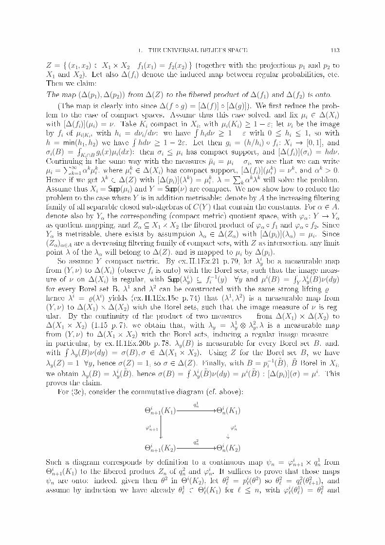
1. THE UNIVERSAL BELIEFS SPACE 113
Z = f (x1, x2) 2 X1 X2 j f1(x1) = f2(x2) g (together with the projections p1 and p2 toX1 and X2). Let also ∆(fi) denote the induced map between regular probabilities, etc.
Then we claim:
The map (∆(p1),∆(p2)) from ∆(Z) to the bered product of ∆(f1) and ∆(f2) is onto.
(The map is clearly into since ∆(f Æ g) = [∆(f)] Æ [∆(g)]). We rst reduce the prob-
lem to the case of compact spaces. Assume thus this case solved, and x µi 2 ∆(Xi)with [∆(fi)](µi) = ν. Take Ki compact in Xi, with µi(Ki) 1 ε; let νi be the image
by fi of µi|Ki, with hi = dνi/dν: we have
Rhidν 1 ε with 0 hi 1, so with
h = min(h1, h2) we haveRhdν 1 2ε. Let then gi = (h/hi) Æ fi : Xi ! [0, 1], and
σi(B) =RKi∩B
gi(x)µi(dx): then σi µi has compact support, and [∆(fi)](σi) = hdν.Continuing in the same way with the measures µi = µi σi, we see that we can write
µi =P∞
k=1αkµki , where µ
ki 2 ∆(Xi) has compact support, [∆(fi)](µ
ki ) = ν
k, and αk > 0.
Hence if we get λk 2 ∆(Z) with [∆(pi)](λk) = µki , λ =
Pkα
kλk will solve the problem.
Assume thus Xi = Supp(µi) and Y = Supp(ν) are compact. We now show how to reduce the
problem to the case where Y is in addition metrisable: denote by A the increasing ltering
family of all separable closed sub-algebras of C(Y ) that contain the constants. For α 2 A,denote also by Yα the corresponding (compact metric) quotient space, with ϕα : Y ! Yαas quotient mapping, and Zα X1X2 the bered product of ϕα Æ f1 and ϕα Æ f2. SinceYα is metrisable, there exists by assumption λα 2 ∆(Zα) with [∆(pi)](λα) = µi. Since
(Zα)α∈A are a decreasing ltering family of compact sets, with Z as intersection, any limit
point λ of the λα will belong to ∆(Z), and is mapped to µi by ∆(pi).So assume Y compact metric. By ex. II.1Ex.21 p. 79, let λiy be a measurable map
from (Y, ν) to ∆(Xi) (observe fi is onto) with the Borel sets, such that the image meas-
ure of ν on ∆(Xi) is regular, with Supp(λiy) f−1i (y) 8y and µi(B) =RYλiy(B)ν(dy)
for every Borel set B. λ1 and λ2 can be constructed with the same strong lifting L
hence λi = L(λi) yields (ex. II.1Ex.15e p. 74) that (λ1, λ2) is a measurable map from
(Y, ν) to ∆(X1) ∆(X2) with the Borel sets, such that the image measure of ν is reg-
ular. By the continuity of the product of two measures from ∆(X1) ∆(X2) to
∆(X1 X2) (1.15 p. 7), we obtain that, with λy = λ1y λ2y, λ is a measurable map
from (Y, ν) to ∆(X1 X2) with the Borel sets, inducing a regular image measure
in particular, by ex. II.1Ex.20b p. 78, λy(B) is measurable for every Borel set B, and,with
Rλy(B)ν(dy) = σ(B), σ 2 ∆(X1 X2). Using Z for the Borel set B, we have
λy(Z) = 1 8y, hence σ(Z) = 1, so σ 2 ∆(Z). Finally, with B = p−1i˜(B), B Borel in Xi,
we obtain λy(B) = λiy˜(B), hence σ(B) =
Rλiy
˜(B)ν(dy) = µi ˜(B) : [∆(pi)](σ) = µi. This
proves the claim.
For (3c), consider the commutative diagram (cf. above):
Θin+1(K1)
q1n!Θi
n(K1)
ϕin+1
????y????yϕi
n
Θin+1(K2)
q2n!Θi
n(K2)
Such a diagram corresponds by denition to a continuous map ψn = ϕin+1 q1n from
Θin+1(K1) to the bered product Zn of q2n and ϕi
n. It suces to prove that those maps
ψn are onto: indeed, given then θ2 in Θi(K2), let θ2 = pi(θ
2) so θ2 = q2(θ2+1), and
assume by induction we have already θ1 2 Θi(K1) for * n, with ϕi
(θ1) = θ2 and

114 III. THE BELIEFS SPACE
q1−1(θ1) = θ
1−1. Then (θ2n+1, θ
1n) 2 Zn, hence the surjectivity of ψn will yield the existence
of θ1n+1 2 Θin+1(K1) with ϕ
in+1(θ
1n+1) = θ
2n+1 and q
1n(θ
1n+1) = θ
1n: we obtain a full sequence
(θ1n)∞n=−1, i.e. a point θ1 2 Θi(K1) with, 8n, pin(θ1) = θ1n, so (ϕi
n Æ pin)(θ1) = pin(θ2) 8n
hence by our diagram in the beginning of the proof of (3), [Θi(f)](θ1) = θ2.We will prove the surjectivity of ψn by induction. So assume n 0, and ψn−1
is onto. Let X in = Ki
Qj =iΘ
jn(Ki), also gn = f
Qj =iϕ
jn : X
1n ! X2n, and
hin = idKiQ
j =i qjn : X
in+1! X i
n. In the commutative diagram:
X1nh1n−1
!X1n−1
gn
????y????ygn−1
X2nh2n−1
!X2n−1the surjectivity of ψn−1 on each of the factors Θj(j 6= i) separately yields that of the
induced map χn = gnh1n−1 from X1n to the bered product Pn of h2n−1 and gn−1. And, by
our diagram in the beginning of the proof of (3), proving the surjectivity of ψn amounts
to prove that in the diagram:
∆(X1n)∆(h1
n−1)
!∆(X1n−1)
∆(gn)
????y????y∆(gn−1)
∆(X2n)∆(h2
n−1)
!∆(X2n−1)
the induced map from ∆(X1n) to the bered product of ∆(h2n−1) and ∆(gn−1) is onto.
But this is the composition of ∆(χn) with the map from ∆(Pn) to the bered product of
∆(h2n−1) and ∆(gn−1). The rst is onto by 9.b.3 [K-analyticity of X1n follows from point
1 of the present theorem, the onto character of pin, theorem 1.1 part 3, and 3.a], and the
second by our above claim.
Comment 1.4. Compactness is clearly necessary in point 2, e.g.,K-analyticity, to gen-
eralise at the same time point (3c), would be far insucient. Consider for example any K-
analytic set K, on which there exists a non-constant continuous function. Then there is a
proper Z -subset, say Z, so by (3a) Θi(Z) is a Z -subset of Θi(K): let Θi0 = Θi(K)nΘi(Z),
Θin+1 = (δi)−1(∆(K Qj =i Θ
jn)). Observe that, using inductively 9.b.2, the Θi
n are Zcδ-
subsets of Θi(K). Further Θi1 Θi
0must clearly be disjoint from Θi(Z), so by induc-
tion the Θin form a decreasing sequence. Let Θi =
Tn Θ
in: clearly δ
i(Θi) = ∆(KQ
j =i Θj),
further the ΘiareZcδ-subsets of Θ
i(K), strictly included in it, and non-empty e.g. because
they contain (induction again) Θi(K n Z).Comment 1.5. The previous comment implies in particular that the homeomorph-
ism between Θiand ∆(K
Qj =i Θ
j) is far from sucient to characterise the spaces
Θi(K) even when the Θiare restricted to be (nice Zcδ) subsets of Θ
i(K). There
is a dierent sense in which too it is insucient and this even with all spaces com-
pact: one can have, with K compact, compact spaces Θiand homeomorphisms σi
from Θito ∆(K
Qj =i Θ
j), without Θibeing in any sense homeomorphic to Θi(K).
For instance, let X1 = [0, 1], Xn+1 = ∆(Xn), q1 : X2 ! X1 maps to the barycentre,

1. THE UNIVERSAL BELIEFS SPACE 115
qn = ∆(qn−1) : Xn+1 ! Xn for n > 1. Obviously the Xn are compact metric, and the
qn continuous and onto (induction). Let X be the projective limit (compact metric), with
projections pn onto Xn. For x 2 X, the pn+1(x) dene a projective system of probabilities
on the Xn(n 1), hence a probability δ(x) 2 ∆(X). The map δ is clearly one-to-one,
continuous, and onto, so a homeomorphism from X to ∆(X) by compactness. Let then,
for I = f1, 2g,#K = 1, Θi = X, with δi a copy of δ, δi : Θi ! ∆(K Θj) (i 6= j). So
our Θi, δi have all required properties for the one-point space K, still are in no sense
homeomorphic to the one-point space Θi(K).
We prove now that property (P ) still holds when the maps are only assumed measur-
able. Actually, our solution does not seem exactly right, since we have to restrict slightly
the class of topological spaces considered: it would be more natural to investigate, for
given spaces, for which class of maps the property still holds, rather than, for a given
measurability concept, what class of spaces can be used.
Theorem 1.3. Assume that in property (P ), the spaces Σi and K are quasi-Ra-don (10.a), and the maps σi and f universally measurable. Then there exist uni-que maps Θi(f) making the diagram commutative in the sense that for every Borel
set B in K Q
j =iΘj such that B = [f
Qj =iΘ
j(f)]−1(B) is σi(si) measurable,
[σi(si)](B) = [δi[(Θi(f))(si)]](B). Those Θi(f) are universally measurable so the dia-gram is unrestrictedly commutative (even for all universally measurable B).
Proof. Is the same as in theorem 1.1, proving inductively that the ϕjn are univer-
sally measurable (and uniquely dened) using 10.a.5, 9.d.1, 10.a.4 and again 9.d.1 at
every step of the induction. Then by induction, we must have pin Æ Θi(f) = ϕin for all n:
Θi(f) is thereby uniquely dened, and its universal measurability follows by writing it as
the composition (9.d.1) of the inclusion of Σias the diagonal of (Σi)∞ and the universally
measurableQ
nϕin : (Σ
i)∞ !QnΘ
in (9.d.1) together with the remark that a universally
measurable map is still universally measurable to every subspace of the image space that
contains the range. Commutativity of the diagram follows now for every Borel set B of
the form (idK Q
j =i pjn)
−1(B) with B Borel, hence by a monotone class argument for all
Borel sets (clearly any open set belongs to this monotone class, being a union of basic
open sets). This extends then immediately to the universally measurable B's.
Comment 1.6. In particular, if two quasi-Radon spaces are universally measurably
isomorphic, one obtains a similar isomorphism between their corresponding systems:
thus, the (Θi(K), δi)i∈I and their universally measurable structure (all universally meas-
urable maps to and from all topological spaces) are uniquely determined by the universally
measurable structure of K: in some sense, the solution is purely measure theoretic.
Also, one encounters often the variant of property (P ) where the map f is replaced
by a transition probability. Then
Theorem 1.4. Assume in property (P ) that K is quasi-Radon, f is a continuous mapto ∆(K), and the maps σi are continuous. Then there are unique (in the same sense as intheorem 1.3) continuous maps Θi(f) making the diagram commutative, where the righthand arrow is interpreted as β Æ [∆(f Qj =iµ
j ÆΘj(f))], with the barycentric map β as
in 10.a and µj : Θj ! ∆(Θj) mapping every point to the unit mass at this point.
Proof. By the continuity of the product of probabilities (1.15 p. 7), and 10.a.6 (the
spaces are quasi-Radon as in theorem 1.2, point 1), the proof is now as in theorem 1.1

116 III. THE BELIEFS SPACE
p. 107 with the modied interpretation of the right hand arrow. Only some more care is
required for the proof that qin Æ ϕin = ϕi
n−1 also follows inductively.
Comment 1.7. With K = ∆(K),Σi = Θi(∆(K)), and f the identity one obtains
the canonical continuous map from Θi(∆(K)) to Θi(K). So in the general case, when fhas values in ∆(K) and all maps are universally measurable, one still obtains the result,
assuming all spaces are quasi-Radon: Θi(f) is universally measurable from Σito Θi(K),
and obtained by composing the map from Σito Θi(∆(K)) obtained in Theorem 1.3 with
the canonical map above from Θi(∆(K)) to Θi(K). Of course, a direct denition, like in
theorem 1.4, is also possible.
Comment 1.8. In the line of the remark after theorem 1.1, there is a category of
quasi-Radon spaces, with universally measurable transition probabilities as morphisms;
indeed, f : X ! ∆(Y ) and g : Y ! ∆(Z) compose as g f = β Æ (∆(g)) Æ f (5.d and 5.f).
Remark 1.7 shows then that Θiis a (covariant) functor from this category to the category
of quasi-Radon systems with universally measurable morphisms.
Corollary 1.5. (1) If K is countably Radon, or analytic, then for any othercountably Radon or analytic topology on K with the same Borel σ-eld or thesame Bu, one obtains another countably Radon or analytic topology on Θ(K),with the same map δ, and with the same Borel σ-eld or same Bu.
(2) Assume K is countably Radon, or analytic.Let (Σi,Si) and (Ω,A ) be measurable spaces, together with a transition
probability Q from (Ω,A ) to K with the Borel sets, and transition probabilitiesσi from (Σi,Si) to (Ω,A )
Qj =i(Σj,Sj). Then there exists a unique system of
measurable maps Θi(Q) from (Σi,Si) to Θi(K) with the Borel sets such that thediagrams of property (P ) commute.
(3) The measurable space Θi(K) with the Borel sets is uniquely characterised by theabove property.
Proof. Apply the above, and 10.b including remark 1.7 p. 116.
In view of theorem 1.1 p. 107 we refer to Θ as the universal type space. It is
determined by K and I only. The space Θiis called the type set of player i.
We dene now the space Ω by: Ω = K Qi∈IΘi. This space is called the universal
beliefs space and its elements are called states of the world.
The denition of Ω and the basic property of the type space: Θihomeomorphic to
∆(K Q
j =iΘj), are the formal expression of Harsanyi's approach in modelling games
with incomplete information namely: A state of the world consists of a state of nature
together with a list of types; one for each player. A type of a player denes a joint
probability distribution on the states of nature and the types of the other players.
Note that our construction is based on some implicit assumptions on the players' be-
liefs: The subject of each player's beliefs are the states of nature and the beliefs of the
others. He `knows' his own beliefs. Second, the denition of the projections ϕin implies
that each level of player i's beliefs is compatible with his lower levels beliefs and he be-
lieves that this is so for all players and so on. An alternative approach is to make the
player's beliefs be on the states of nature and all lower levels beliefs, including his own.
If we do so then the above mentioned coherency conditions become explicit restrictions
on the admissible beliefs. This is done in ex. IIIEx.2 p. 141.

1. THE UNIVERSAL BELIEFS SPACE 117
Given θ 2 Θi, let θ = δi(θ) εθ 2 ∆(Ω) where εθ is the unit mass at θ. Recall
that the product of regular probabilities is a continuous map (1.15 p. 7): the map θ 7! θis continuous. So is the projection map θi : Ω ! Θi
, and hence also the map ω 7! θiωfrom Ω to ∆(Ω). θi(ω) or (θiω) is referred to as the type of player i at !. Note that
if ω 2 Supp(θiω) then θiω = θiω. In words: at any state of the world, each player knows his
own type.
1.b. Beliefs subspaces. The universal beliefs space Ω consists of all possible inform-
ational congurations regarding K. Any private or public information about K may
restrict the conceivable states of the world to a subset of Ω containing all the beliefs of
all players. This motivates the following denition.
Definition 1.6. A beliefs subspace (BL-subspace) is a non-empty subset Y of Ωwhich satises:
8ω 2 Y , θiω(Y ) = 1 8iA point of a BL-subspace Y can be written as ω = (k; θ1(ω), . . . , θi(ω), . . . ). The set
θi(Y ) is the type set of player i in the BL-subspace Y . Clearly Ω itself is a BL-subspace.The following are examples of BL-subspaces corresponding to well known classes of
games.
(1) Games with complete information.
For xed k 2 K let Y = fωg where ω = (k; εω, . . . , εω), and εω is the measure
on Y assigning unit mass to ω. This is a usual situation of complete information.
(2) Games with a random move to choose the state of nature.
For k1 and k2, two distinct elements in K, let
Y = fω1, ω2gω1 = (k1; (p, 1 p), . . . , (p, 1 p))ω2 = (k2; (p, 1 p), . . . , (p, 1 p))
Here there is only one type of each player: (p, 1 p) which assigns probability pto ω1 and (1 p) to ω2. This is a situation in which a random move chooses the
state of nature k1 or k2 with probabilities (p, 1 p).In the following examples there are two players, I and II and the elements of
K are games denoted by G1, G2, . . . or G12, G22, . . . etc.(3) Games with incomplete information on one side.
Y = fω1, . . . , ωKg where for k = 1, . . . ,K,
ωk =Gk; εωk
, (p1, . . . , pK)
That is, the game Gk 2 fG1, . . . , GKg is chosen according to the probability vec-
tor p = (pk)k∈K. Player I is informed which game was chosen and player II isnot.
(4) Games with incomplete information on 112 sides (cf. ex. VIEx.8 p. 318).
Y = fω1, ω2, ω3g where
ω1 =G1; (1/3, 2/3, 0), (1, 0, 0)
ω2 =
G1; (1/3, 2/3, 0), (0, 1/2, 1/2)
ω3 =
G2; (0, 0, 1), (0, 1/2, 1/2)

118 III. THE BELIEFS SPACE
To see the main feature of this BL-subspace assume that the actual state of the
world is ω2. While player I knows that the game is G1, he is uncertain about the
state of mind of player II; whether he knows that it is G1 (state ω1) or his beliefsare (1/2, 1/2) (state ω2). Player I assigns to these two possibilities probabilities
1/3 and 2/3 respectively.
(5) Incomplete information on two sides: the independent case.
Y = fω11, ω12, ω21, ω22g where
ω11 =G11; (1/2, 1/2, 0, 0), (1/3, 0, 2/3, 0)
ω12 =
G12; (1/2, 1/2, 0, 0), (0, 1/3, 0, 2/3)
ω21 =
G21; (0, 0, 1/2, 1/2), (1/3, 0, 2/3, 0)
ω22 =
G22; (0, 0, 1/2, 1/2), (0, 1/3, 0, 2/3)
Player I can be of two types: I1 = (1/2, 1/2, 0, 0) or I2 = (0, 0, 1/2, 1/2) whileplayer II can be either of type II1 = (1/3, 0, 2/3, 0) or II2 = (0, 1/3, 0, 2/3).Note that each player knows his own type. An equivalent description of this
informational structure is the following: Chance chooses a pair of types from
fI1, I2g fII1, II2g according to the probability distribution:
II1 II2I1 1/6 1/6I2 1/3 1/3
If the selected pair of types is (Ir, IIs), each player is informed of his type (only)
and then they proceed to play the game Grs. Note that in this representation
the types of the players are chosen independently.
(6) Incomplete information on two sides: the dependent case.
Y = fω11, ω12, ω21, ω22g where
ω11 =G11; (1/2, 1/2, 0, 0), (1/3, 0, 2/3, 0)
ω12 =
G12; (1/2, 1/2, 0, 0), (0, 1/7, 0, 6/7)
ω21 =
G21; (0, 0, 1/4, 3/4), (1/3, 0, 2/3, 0)
ω22 =
G22; (0, 0, 1/4, 3/4), (0, 1/7, 0, 6/7)
This situation can be interpreted and represented in the same way as the previous
example with the joint probability on types being:
II1 II2I1 1/10 1/10I2 1/5 3/5
Thus, unlike the previous example, the types of the two players are not inde-
pendent.
(7) Incomplete information on two sides: the inconsistent case.
Consider a variant of the previous example in which the second type of player
II is II2 = (0, 1/5, 0, 4/5) instead of (0, 1/7, 0, 6/7). With this modication the
players' beliefs can no longer be viewed as conditional distributions, given each
player's type, derived from some prior joint distribution on fI1, I2g fII1, II2g.

1. THE UNIVERSAL BELIEFS SPACE 119
Such situations of incomplete information are called inconsistent cases (cf. ex-
ample in the next section).
The following are some general constructions of beliefs subspaces.
(1) Any union of beliefs subspaces is one.
(2) In particular, the union Ωf of all nite beliefs subspaces.
(3) Any countable intersection of beliefs subspaces is one.
(4) Any intersection of closed beliefs subspaces is one.
(5) In particular, 8ω 2 Ω there is a smallest closed beliefs subspace containing ω. Itis obvious how to construct it directly (by possibly transnite induction . . . ).
(6) (a) As a cautionary remark, observe that one could also use in 4 above separ-
ately closed, in the sense that a subset is separately closed if the inverse
image of every point in any factor Θi(i 2 I) is closed. One obtains thus alsoan analogous statement to 5, but associating with every ω 2 Ω a typically
smaller BL-subspace.(b) In the same vein, one could also dene a concept of topological
BL-subspace by requiring that 8ω 2 Y , 8i 2 I, Supp(θiω) Y . Clearly, topo-
logical BL-subspaces are closed under arbitrary unions and intersections. In
particular, for every ω 2 Ω there is a smallest topological BL-subspace con-taining it which should be (typically) even smaller than the one obtained
sub 6a.
(7) Given Ω0 Ω, let Ωn+1 = fω 2 Ωn j θiω(Ωn) = 1 8i 2 I g. Then Ω∞ =
TnΩn is a
beliefs subspace. It is the subspace where Ω0 is common knowledge.
(a) Ω∞ is the maximal (cf. 1) beliefs subspace contained in Ω0.(b) When Ω0 is closed, or a Gδ, (or Borel, or universally measurable, or has any
of the properties mentioned in theorem 1.2 part 1 p. 111), then so is Ω∞.(c) Observe that the above generalises theorem 1.2 part 3b p. 111. Cf. also
ex. IIIEx.3 p. 142 for another application.
(8) Let Ω0 = fω 2 Ω j ω 2 Supp(θiω) 8i 2 I g.
(a) If Ω is metrisable, then Ω0 is a Gδ in Ω. Indeed, for a metric space E, theset f (e, µ) 2 E ∆(E) j d(e, Supp(µ)) ε g is closed.
(b) In particular by 6b and Theorem 1.2 part 1 p. 111, if K is separable metric,
then Ω∞ is a Gδ.
Comment 1.9. It is the beliefs subspace where it is common knowledge that
no player believes a neighbourhood of the true state to be impossible. Consider an
interpretation of Ω as a model for modal logic, where (Borel) subsets of Ω would
correspond to propositions, and where Bi(p) player i believes p would be
interpreted as θiω assigns probability one to the (Borel) set p. Observe that, whenp is a closed set, Bi(p) is one too. Restricting the model to Ω∞ corresponds then
to require the beliefs-operators to be knowledge operators on closed sets. (One
could also restrict propositions to the Boolean algebra generated by the closed
sets.) (Thus, independently of the class of subsets to which one restricts proposi-
tions, there is a variant concept of Bi(p) behind the scenes, which is that player
i assigns probability one to some closed subset of p.)
Other examples will be given in the next section.

120 III. THE BELIEFS SPACE
2. Consistency and common knowledge
The types of the players at a given state ω are probability distributions (beliefs) on
Ω. A natural question is: Can these be conditional probability distributions derived from
some prior probability on Ω given the players' types?
Definition 2.1. A probability distribution Q 2 ∆(Ω) is consistent if for all i 2 Iand every Borel set B of Ω;
(1) Q(B) =
ZΩ
θiω(B)Q(dω)
In words: Q is consistent if it equals the average (according to Q) of each of the beliefsθiω. The following lemma proves that denition 2.1 indeed captures the intuitive meaning
of consistency.
Lemma 2.2. If Q 2 ∆(Ω) is consistent then for all i 2 I, and for any Borel oruniversally measurable subset A of Ω,
(2) θiω(A) = Q(A j T i)(ω) Q-a.e.
where T i is the sub σ-eld on Ω generated by θi and the Borel or universally measurable σeld on Θi.
Proof. We have to prove that for any measurable set A in Ω and for any B 2 T i:Z
B
θiω(A)Q(dω) =
ZB
1AQ(dω) .
The right hand side is equal to Q(A\B) so that the equation will follow from (1) (applied
to the measurable set A \ B) if we show that 1B(ω)θiω(A) = θ
iω(A \ B) for any B 2 T i
.
This follows from the fact that θi is constant on the support of θiω, so that the full supportis either in B or disjoint from B.
Comment 2.1. If K is completely regular, it suces already that equation (1) be sat-
ised for bounded continuous functions instead of Borel sets. Indeed, since the completely
regular spaces are the subspaces of compact spaces, Θiand hence Ω are then completely
regular too, so the equation passes from continuous functions to indicator functions of
compact sets (regularity of Q and θiω), and then to Borel sets (regularity of Q).
Comment 2.2. Equation (1) remains valid with non-negative universally measurable
functions instead of the Borel set B.
Denote by P the set of all consistent probabilities on Ω.
Theorem 2.3. The set P is closed and convex in ∆(Ω).
Proof. Convexity of P is obvious equation (1) is linear. Let thus Pα 2 P con-
verge to P 2 ∆(Ω). Let µ(B) =Rθiω(B)P (dω). Observe that, for any compact set C,
µ(C) = inffµ(O) j O closure of an open set O containing C g. Indeed, since Ω is T2 andC compact, the intersection of those sets O equals C so the θiω(O) form a decreasing
net of u.s.c. functions converging to θiω(C) (regularity of θiω), hence, by the regularity of
P , µ(O) decreases to µ(C).By the upper semi-continuity of θiω(O), lim supα
Rθiω(O)Pα(dω)
Rθiω(O)P (dω), i.e.,
lim supαPα(O) µ(O). But also lim inf Pα(O) P (O) P (C). Hence P (C) µ(O)for every O, so P (C) µ(C) for every compact set C. The regularity of P implies then
P = µ.

2. CONSISTENCY AND COMMON KNOWLEDGE 121
Corollary 2.4. All topological properties of K mentioned in theorem 1.2.1 p. 111are inherited by Ω and by P .
Proof. By theorem 1.2.1, they are inherited by Θi and by ∆(K), by countable
products and by closed subspaces. Therefore they are also inherited by Ω = K Q
iΘi,
hence by ∆(Ω), hence by the closed subspace P of ∆(Ω).
In general, a BL-subspace will fail to have a consistent distribution.
Example 2.3. Consider a situation of two players each of which has two types. The
BL-subspace Y has four points corresponding to the four possible couples of types:
Y =
11 1221 22
At each point of Y (an entry of the matrix), the rst digit denotes the type of player Iand the second is that of player II. Similarly we denote the subjective probabilities of the
players by:
For I:
II1 II2I1 p1 1 p1I2 p2 1 p2
For II:
II1 II2I1 q1 q2I2 1 q1 1 q2
It is easily veried that there is a consistent distribution i q1(1 p1)/[p1(1 q1)] =q2(1 p2)/[p2(1 q2)].
Examples on BL-subspaces (continued).
(1) If K is a separable metric space, or is analytic, so is P (cor. 2.4). Hence P has
a countable dense sequence (Pn)∞n=1. By theorem 2.3, P∞ =
P∞1 2−nPn belongs
to P . Further Supp(Pn) Supp(P∞). Since the sequence Pn is dense, we obtain
Supp(P ) Supp(P∞)8P 2 P : The set of supports of consistent probabilities has
a maximal element (Supp(P∞)), say S. Even for general K, one can always dene
S as [f Supp(P ) j P 2P g.(2) For any P 2 P , Supp(P ) is a (closed) BL-subspace. This can be combined with
the constructions of sect. 1.b, like 2, 3, 4, or 8a to yield other BL-subspaces.(3) A variant of 5 p. 119 becomes now available, assuming K compact: For every
decreasing net of supports of consistent probabilities, the intersection contains a
minimal such set (using compactness of P).
(4) Given Ω0 as in example 7 p. 119, and P 2P , if P (Ω0) = 1, then P (Ω∞) = 1.(5) With Ω0 as in example 8a p. 119, and P 2P , one has P (Ω0) = 1.(6) Combining all the above, let S0 = S \Ω∞, with Ω∞ as in example 8a p. 119, and
S as in example 1 above. Then S0 is a canonical BL-subspace, with P (S0) = 1,8P 2 P , and expresses common knowledge of both consistency of beliefs and
that nobody believes a neighbourhood of the true state to be impossible.
(7) Assume K is standard Borel. So by Corollary 1.5 p. 116 the Borel spaces ΘiK are
uniquely determined, and are standard Borel too.
(a) By ex. II.1Ex.9 p. 60, there exists for every player i a Borel measurable
transition probability qi(dk j θ) fromQ
j Θjto K, such that for every
θi 2 Θi, and every non-negative Borel function f on Ω,
RΩf(ω)θ(dω) =R R
f(k, θ−i, θi)qi(dk j θ−i, θi)θi(dθ−i) i.e. qi is the conditional probab-
ility on K given θ, under the distribution θi. Indeed, use E = Θi, Y =
Θ−i(=Q
j =iΘj), X = Y K, and g the projection. And since g(e, x) is onto

122 III. THE BELIEFS SPACE
8e 2 E, we can obtain in II.1Ex.9c p. 60 that Q(fx j g(e, x) = y g j e, y) = 18e, 8y, by modifying Q on the negligible set. Therefore Q can be viewed as
a transition probability from E Y to K.
(b) It follows that qi is also, 8P 2 P , a version of the conditional probability
on K given θ 2Q
j Θj. In particular, Ω0 = f θ j qi = qj8i, j g is a Borel set
with P (Ω0) = 1 8P 2P .
(c) Thus, the corresponding beliefs space Ω∞ is a Borel subset ofQ
iΘi, with
P (Ω∞) = 1 8P 2P , and there is a Borel measurable transition probability
q from Ω∞ to K which is a version of the conditional probability on K givenQiΘ
iunder every P 2P , and under every θ
iω, 8i 2 I and 8ω 2 Ω∞.
(d) In the two player case, one could do a bit better: Modify q1 by setting it
equal to q2 on Θ10Θ2, where Θ10 = f θ1 j θ1(Ω0) = 1 g. Do then the same with
q2 and Θ20. (Instead of iterating the procedure, into the transnite?), one
can now choose for Ω0 the set Θ10Θ20, and obtain then a similar product set
Θ1∞Θ2∞ for Ω∞. Using remark 1.2 p. 110, one can now symmetrise the situ-
ation under permutations of the players, and obtain a single Borel set Θ∞,which has probability one under any θ 2 Θ∞, such that Θ∞Θ∞ has prob-
ability one under every P 2P , and a single Borel transition q(dk j θ1, θ2) on(Θ∞Θ)[ (ΘΘ∞), which is symmetric in (θ1, θ2), and is the conditional
probability under any P 2P and under θ 2 Θ∞. And when K is nite, one
could further symmetrise under all permutations of K.
Comment 2.4. Are there any canonical results in this vein? E.g., does the union
of such beliefs spaces cover the set S? Is there a canonical such beliefs space even
replacing Borel-measurability by universal-measurability, or by µ-measurability for every
consistent prior and for each belief in the beliefs space?
Comment 2.5. The above is frequently used, in the context of sect. 4 below. In that
case, to every k 2 K there corresponds a game (pay-o functions) gk. Averaging them
under such a common conditional q yields a model where one has a single game for every
I-tuple of types. If further the (consistent) joint distribution is absolutely continuous onQi∈IΘ
iw.r.t. some product measure then it is a.c. w.r.t. the product of its margin-
als , one can, using f(θ) for its density with respect to the product of the marginals,
replace every every game gθ by f(θ)gθ. In this way, one obtains a model (information
scheme as below) where furthermore all players' private signals are independent. It would
seem worthwhile to check what such transformations yield for the corresponding canonical
consistent distributions (theorem 2.5 part 2 below).
Information Schemes. In games with incomplete information, the information
structure is dened by an information scheme, I , that consists of a probability space
E = (E, E , Q) and sub σ-elds E i(for each i in I), with a measurable mapping kE from E
to the spaceK of states of nature. The sub σ-eld E idescribes the information of player i.
The following theorem states that any information scheme has a canonical representation
as a consistent probability measure on Ω. Denoting by k the canonical projection from Ωto K we have:
Theorem 2.5. Assume an information scheme I such that kE is Borel-measurableand Q has a regular image measure µ.
(1) Then there exists a Q-measurable map ϕ from (E, E ) to Ω with the Borel setssuch that:

2. CONSISTENCY AND COMMON KNOWLEDGE 123
(a) (k Æ ϕ)−1(B) = (kE)−1(B) Q-a.e., for every Borel subset B of K.
(b) Q Æ ϕ−1 2P [or just: 2 ∆(Ω)].(c) θi(ϕ(e))(B) = (Q[ϕ−1(B) j Ei])(e) Q-a.e., for every Borel subset B of Ω and
all i 2 I.(2) If ϕ is another such map, then ϕ−1(B) = ϕ−1(B) Q-a.e., for every Borel set B of
Ω. (In particular, Q Æ ϕ−1 is uniquely dened).(3) Assume there exists K0 K with µ(K0) = 1 such that points of K0 are separated
by some sequence of µ-measurable sets. Then:(a) Point 2 implies that ϕ = ϕ Q-a.e.(b) In (1a) one can require k Æ ϕ = kE.(c) One can further require that θi(ϕ(e)) is E i-measurable.
Proof. During the proof of (1) and (2) we will assume E icontains all negligible
subsets of (E, E , Q). We start with the following:
Lemma 2.6. Let ϕ and ϕ two random variables on a probability space (Ω,B, P ) withvalues in a measurable space (S,S ).
(1) Assume S is completely regular and S the Borel σ-eld, the distributions of ϕand ϕ are regular, or just τ -smooth (cf. 10.a) and that for every real boundedcontinuous function f on S, f Æ ϕ = f Æ ϕ a.e. Then the same holds true for anyreal Borel function f .
(2) AssumeS separable and separating and that for every T 2 S , ϕ−1(T ) = ϕ−1(T )a.e., then ϕ = ϕ a.e. If A B is such that every element of B is a.e. equal tosome element of A then there exists ϕ which is A -measurable and is a.e. equalto ϕ.
Proof. 1. Going to the Stone-ech compactication, one can assume the image space
is compact. One obtains then rst, by a monotone class argument, that f Æ ϕ = f Æ ϕa.e. for every Baire function f . So the distributions coincide on the Baire σ-eld, hence(regularity) on all compact sets, since those have a basis of open Baire neighbourhoods,
hence (regularity) on all Borel sets. Let P be this distribution. For K compact, let On be,
as just said, an open Baire set withK On, P (OnnK) n−1; let K =T
nOn: K is a Baire
set with K K, P (K nK) = 0. Hence ϕ−1(K) =a.e. ϕ−1(K) =a.e ϕ
−1(K) =a.e. ϕ−1(K).
so we still have ϕ−1(C) = ϕ−1(C) a.e., for every Kσ-set C. The same conclusion follows
now in the same way for Borel sets, approximating them by regularity from inside by
Kσ-sets. Hence the result.
2. Let Tk be a sequence of generators of S , and neglect the points where, for some
k, ϕ−1(Tk) 6= ϕ−1(Tk). Now (ϕ, ϕ)−1(Rk) = φ with Rk = [Tk Tk] [ [Tk Tk]. SinceSkRk is the complement of the diagonal in S S, the rst assertion follows. For the
second, reduce to the case where (S,S ) is a subset of [0, 1] with the Borel subsets and
approximate ϕ uniformly by a sequence of step functions ϕn and let ϕ = lim inf ϕn.
For the theorem, we rst reduce the proof of (1) and (2) to the case where K is com-
pact. Find a sequence Cn of disjoint compact subsets of K with µ(S
nCn) = 1. Denote by
K the (locally compact) disjoint union of the Cn, and by K its one-point compactication.
For point (2), observe rst that ϕ (and ϕ) can be modied on a null set such as to have
values in Ω⋃nCn
ΩK, by theorem 1.2 part 3b p. 111. Indeed, assume ϕ has already been
modied such as to have values in [(S
kCk) (An)I], then, taking for B the latter subset
in 1c, we get that θiϕ(e)(B) = 1 a.e. hence the induction step. Next, since K is a Zc-set

124 III. THE BELIEFS SPACE
in K, ΩK is a Zcδ set (theorem 1.2 part 3a p. 111 in the compact space (theorem 1.2
part 1) ΩK, hence K-Lusin (3.d, 3.e). Hence the map from ΩK to Ω⋃nCn
is continuous,
one-to-one and onto (theorem 1.2 parts 3a and 3c p. 111). Therefore ϕ and ϕ still have
the same properties when viewed as maps to ΩK by (9.b.4 and 9.b.3). And clearly kE can
be viewed as K-valued. Finally, theorem 1.2 part 3a allows to assume that the values are
in ΩK and in K.
For point 1 of theorem 2.5, our assumptions are clearly still satised with K instead
of K. Obtaining thus an appropriate ΩK-valued ϕ, and letting B0 = fω 2 ΩK j kω 2 K g,Bn+1 = fω 2 Bn j θiω(Bn) = 1 8i g, then, by theorem 2.5 parts 1a and 1c and inductively,
we get Q(ϕ−1(Bn)) = 1 8n, hence, after modifying ϕ on a null set, ϕ : E ! ΩK =T
nBn
(theorem 1.2 part 3b). So, by theorem 1.2 part 3a, composing ϕ with the continuous
one-to-one map from ΩK to ΩK will yield the desired result. Hence, for parts 1 and 2 of
the theorem we can assume K compact.
We now start the proof of 1. Let L be a lifting on (E, E , Q); and let k = L(kE)(ex. II.1Ex.15e p. 74). Then, by the above lemma, we have k−1
E (B) = k−1(B) Q-a.e., forevery Borel set B. So it suces to prove 1 with k instead of kE i.e., we can assume
that kE = L(kE). Assume, for n 1, that ϕn = (kE, (tin)i∈I) : E ! Ωn = K QiΘ
in is
well-dened, and Q-measurable, such that ϕn = L(ϕn) hence ϕn is measurable to the
Borelσ-eld, withQÆϕ−1n 2 ∆(Ωn), by (ex. II.1Ex.15eiii p. 75) , and such that tin(e)(B) =
E[(ϕin−1)
−1(B) j Ei](e) Q-a.e., for every Borel subset B of X in−1 = K
Qj =iΘ
jn−1, where
ϕin = ProjXi
nÆϕn. Assume nally that ϕn−1 = ProjΩn−1
Æϕn, where ProjΩn−1= idK
Qi q
in.
Map then Q to its image on (E, Ei) X in and apply II.1Ex.16c to this image measure,
yielding an Ei-measurable map tin+1 to Θin+1 = ∆(X i
n), such that tin+1 = L(tin+1). Then
ϕn+1 = (kE, (tin+1)i∈I) : E ! Ωn+1 satises ϕn+1 = L(ϕn+1) by ex. II.1Ex.15eiv p. 75. By
denition tin+1(e)(B) = E[(ϕin)
−1(B) j Ei](e) Q-a.e. for every Borel set B of X in. In partic-
ular, for B Borel in X in−1, and h
in : X
in ! X i
n−1 the projection, we have
[qin+1(tin+1(e))](B) = t
in+1(e)[(h
in)
−1(B)]
= E[(hin Æ ϕin)
−1(B) j Ei](e)= E[(ϕi
n−1)−1(B) j Ei](e) = tin(e)[B] Q-a.e.
So, as maps into∆(X in−1), for every continuous linear functional ψ, we have ψÆqin+1Ætin+1 =
ψ Æ tin Q-a.e. Hence, by the Stone-Weierstrass theorem, the same holds true for any
continuous function ψ on ∆(X in−1). Therefore, by ex. II.1Ex.15ei and II.1Ex.15eii p. 75
L[qin+1 Æ tin+1] = L(tin) = tin. But by ex. II.1Ex.15eiv, L(qin+1 Æ tin+1) = qin+1 Æ L(tin+1) =qin+1 Æ tin+1. So tin = qin+1 Æ tin+1, and hence ϕn = ProjΩn
Æϕn+1. This nishes the in-
duction step. So we have 8i, ti(e) = (tin(e))∞−1 an E i
-measurable map to (Θi, Borel
sets) by the relation tin−1 = qin Æ tin and because the Borel σ-eld of Θiis gen-
erated by the projections pin (since every closed set F equalsT
n pin(F ) by denition
of the product topology). Also ti = L(ti) by ex. II.1Ex.15eiv p. 75, and so similarly
ϕ = (kE, (ti)i∈I) = L(ϕ) : E ! Ω. In particular, those maps are Borel measurable with
Q Æϕ−1 2 ∆(Ω). Further, for every Borel set B in X in, with ψ
in the projection from X i
to
X in, we have t
i(e)[(ψin)
−1(B)] = E[(ϕi)−1[(ψin)
−1(B)] j Ei](e) Q-a.e. By our above remark
concerning the Borel σ-eld on a projective limit, we obtain thus by a monotone class
argument that [since ti(e) = δi(θiϕ(e))], for every Borel set B in X i,
δi(θiϕ(e))[B] = E[(ϕi)−1(B) j Ei](e) Q-a.e.

2. CONSISTENCY AND COMMON KNOWLEDGE 125
i.e., θiϕ(e)(B) = E[ϕ−1(B) j Ei](e) Q-a.e., for every set B = Θi B, with B Borel in X i.
Or, since θiϕ(e) is Ei-measurable, we get, for any Borel sets B1 in Θiand B2 in X
ithat
θiϕ(e)(B1B2) = 1θiϕ(e)
∈B1θiϕ(e)(ΘiB2) = 1θi
ϕ(e)∈B1
E[ϕ−1(ΘiB2) j Ei](e)= E[1θi
ϕ(e)∈B1
1ϕ(e)∈Θi×B2j Ei](e) = E[ϕ−1(B1B2) j Ei](e) Q-a.e.
By additivity, the same formula remains then true for nite disjoint unions of sets B1B2,and then by a monotone class argument we still get
θiϕ(e)(B) = E[ϕ−1(B) j Ei](e)for every set B in the product of the Borel σ-elds on Θi
and on X i. Now, θiϕ(e), as
the composition of the continuous map ω 7! θiω (cf. supra) and of the map ϕ satisfying
ϕ = L(ϕ), is a map from (E, Ei) to ∆(Ω) with the Borel sets that satises θiϕ(e) = L[θiϕ(·)](e)
and has a regular image measure (ex. II.1Ex.15eiii and II.1Ex.15eiv p. 75). This one has
a barycentre P 2 ∆(Ω) since, by 10.a.2, the compact space Ω is quasi-Radon. I.e.,
for every Borel set B in Ω, θiϕ(e)(B) is measurable andRθiϕ(e)(B)Q(de) = P (B). Also
Q Æ ϕ−1 = P 2 ∆(Ω), i.e., for every Borel set B, P (B) =R
E(ϕ−1(B) j Ei)dQ. Similarly,
for A 2 E , let PA(B) =RAθiϕ(e)(B)Q(de) and PA(B) =
RA
E(ϕ−1(B) j Ei)dQ: since PA Pand PA P , both are regular measures, which coincide by our previous formula on the
product of the Borel σ-elds on Θiand on X i
. By regularity, this implies that they coin-
cide on all compact sets since those have a basis of open neighbourhoods belonging to
the product σ-eld , and hence on all Borel sets. Thus, for every Borel set B in Ω, wehave that Z
A
θiϕ(e)(B)Q(de) =
ZA
[E(ϕ−1(B) j Ei)]dQ 8A 2 E .
This means the two measurable functions are equal a.e.: hence 1c p. 123. By 1c we
have, for B Borel, P (B) = Q(ϕ−1(B)) =R
E(ϕ−1(B) j Ei)dQ =Rθiϕ(e)(B)Q(de) =R
θiω(B)P (dw). Since also P 2 ∆(Ω), this yields 1b: point 1 is fully proved.
For point 2, denote by pn the projection from Ω to Ωn. Assume that ϕ−1[p−1n (B)] =ϕ−1[p−1n (B)]Q-a.e., for every Borel set B in Ωn. [By 1a, this inductive assumption holds for
n = 1]. Then by 1c we obtain that θiϕ(e)(p−1n (B)) = θiϕ(e)(p
−1n (B)) Q-a.e., for every such
B. Let thus Pe = θiϕ(e)Æp−1n , Pe = θ
iϕ(e)Æp−1n , both 2 ∆(Ωn): then Pe(B) = Pe(B) Q-a.e., 8B
Borel. Hence for every continuous linear functional ψ on ∆(Ωn) we have ψ Æ Pe = ψ Æ Pe
Q-a.e., so, by Stone-Weierstrass, this remains true for every continuous function ψ on
∆(Ωn). Take now a continuous function F on Ωn+1 = KQ
iΘin+1 it is, by Stone-Wei-
erstrass again, approximated by linear combinations of functions F = f0 Q
iψi, where
f0 2 C(K) and ψi is continuous on Θin+1 = ∆(X i
n). Hence F Æpn+1Æϕ = f0(kE Æϕ)Q
iψi
(ProjXin(P i)) here the argument of ψi equals ProjXi
n(P i) = ProjXi
n(θiϕ(e) Æ p−1n ) = θin+1(e).
Since ψi Æ ProjXinis continuous on ∆(Ωn), we obtain equality a.e. when replacing ϕ by ϕ.
So F Æ pn+1 Æ ϕ = F Æ pn+1 Æ ϕ Q-a.e., for every F 2 C(Ωn+1). Therefore, by the lemma,
ϕ−1[p−1n+1(B)] = ϕ−1(p−1n+1(B)) Q-a.e., for every Borel set B in Ωn+1. This completes the
induction. It follows that, 8n, 8F 2 C(Ωn), (F Æ pn) Æ ϕ = (F Æ pn) Æ ϕ Q-a.e. Since the
functions F Æ pn are dense in C(Ω) (Stone-Weierstrass), the lemma yields us nally that
ϕ−1(B) = ϕ−1(B) Q-a.e., for every Borel set B in Ω. This proves point 2.As for 3, we rst prove the following claim:
Under the assumptions of 3, there exists a sequence of disjoint compact metric subsetsKn of K such that µ(
SnKn) = 1.

126 III. THE BELIEFS SPACE
Let Ck be a sequence of disjoint compact subsets of K0, with µ(S
kCk) = 1 hence
we can assume K0 =S
kCk. Let also Mn be the sequence of µ-measurable sets. Then
Mn \ Ck diers from some Baire subset Bn,k of Ck by a negligible set Nn,k. Let fk,i be asequence of continuous functions on Ck that generates all Bn,k(n = 1, 2, . . . ). Let also Ck,j
be a sequence of disjoint compact subsets of Ckn(S
nNn,k) with µ(S
jCk,j) = µ(Ck). Then
the points of Ck,j are separated by the sequence of continuous functions fk,i(i = 1, 2, . . . ),so Ck,j is metrisable, and µ(
Sk,jCk,j) = 1.
So let, L =S
nKn. Then L is Lusin (e.g., 5.f), so ΩL ΩK is Lusin too (points 1 and 3
of theorem 1.2 p. 111). Further, as observed in the beginning of the proof of the theorem,
ϕ (and ϕ) can be modied on a null set such as to have values in ΩL and similarly kE
can be assumed to have values in L. The result follows then from point 2 of lemma 2.6
p. 123 (separability is by denition App.5). This nishes the proof of theorem 2.5
Comment 2.6. To facilitate the interpretation of 1a and 2 of theorem 2.5 p. 122,
if ϕ and ϕ are two Borel measurable functions from a probability space to a Hausdor
space X, which have regular image measures and are such that, for every Borel set B,ϕ−1(B) = ϕ−1(B) a.e., then the distribution of (ϕ, ϕ) on XX endowed with the product
of the Borel σ-elds is the restriction to this σ-eld of some regular measure carried by
the diagonal.
Comment 2.7. If there exists a strong lifting for (K,µ) (ex. II.1Ex.15d p. 74), one can
replace 1a p. 123 by k Æ ϕ = kE. Indeed, composing this lifting with the map kE yields a
lifting on a sub σ-eld of (E, E ), which can then be extended to a lifting L for (E, E , Q)[cf. (proof of) II.1Ex.15a p. 74]. For this lifting, one will have L(kE) = kE a.e. they
dier only on the negligible set where kE takes values outside the support of µ. Hence
one obtains, at the end of the construction, that k Æ ϕ = kE Q-a.e.. Changing the K-
coordinate of the map ϕ on the exceptional set yields then the result. But the condition
in (II.1Ex.15d p. 74) for the existence of a strong lifting is (cf. above claim) equivalent to
the condition of theorem 2.5.3 p. 123 where our direct argument yields more.
Comment 2.8. One can always, at the end of the construction, change the K-
coordinate of ϕ and set it equal to kE obtaining thus a map ϕ. However in the
conclusions ϕ−1is then restricted to the product of the Borel σ-eld on K and that onQ
i∈IΘi.
The notion of BL-subspace is closely related to that of consistency and common know-
ledge. In the remainder of this section we study these relations. In doing this we shall
consider from now on only nite BL-subspaces, and assume that all beliefs θiω we use
have nite support, i.e., we restrict ourselves to the space Ωf of Example 2 p. 119.
Definition 2.7. A BL-subspace Y is consistent if there is a consistent distribution
P with Supp(P ) = Y .
Definition 2.8. A state of the world ω 2 Ω is consistent if it belongs to some
consistent BL-subspace i.e., to Ωf \ S.Lemma 2.9. If ω is consistent then ω 2 Supp(θiω) 8i 2 I.
Proof. Let ω 2 Y and P 2 P such that Supp(P ) = Y . Since P (ω) > 0 and
ω 2 T i(ω) = f ω j θi(ω) = θi(ω) g it follows that θiω(ω) = P (ω j T i(ω)) > 0.
The term common knowledge is often used in game theory (including in this book)
in an informal sense: Something is common knowledge among the players if every player

2. CONSISTENCY AND COMMON KNOWLEDGE 127
knows it, every player knows that every player knows it, every player knows that every
player knows that every player knows it, etc. The most intuitive way to think of a common
knowledge event is as an event which is announced (or shown) publicly. A formal deni-
tion of common knowledge was provided in (Aumann, 1976): A measurable space (Y,Y )of states of the world is given together with sub σ-elds Y i
of Y , one for each player. An
event A is common knowledge at ω if there exists B 2 Ti∈IYiwith ω 2 B A.
In our model which is a model of beliefs, the natural analogue for player i believes A
at ω is θiω(A) = 1. And he would know A if further ω 2 A. In particular player believes
A does not necessarily imply that A is true. And of the knowledge operator as dened
is somehow pathological, since when a player believes A, he has no way to know whether
he actually knows it. This is because we did not impose any consistency conditions on
the players' beliefs. To illustrate this consider the following BL-subspace.
Example 2.9. In a two-player situation let Y = fω1, ω2, ω3g whereω1 = (k1; (1, 0, 0) , (0, 1, 0))
ω2 = (k2; (1, 0, 0) , (0, 1, 0))
ω3 = (k3; (1, 0, 0) , (0, 1, 0))
If the true state of the world is ω3 then player I believes that the state of nature is
k1, player II believes that it is k2 while the true state of nature is k3. This extremely
inconsistent beliefs system which can be found in the universal BL-space does not make
sense as a usual knowledge system. Nevertheless we can use this notion of beliefs to
derive what each player i believes to to be common knowledge.
For ω 2 Y and i 2 I dene: Ciω,1 = Supp(θiω), and inductively for r = 1, 2, . . .
Ciω,r+1 = C
iω,r [
[ω∈Ci
ω,r
[j
Supp(θjω).
The interpretation of this sequence is straightforward: According to player i's beliefs at ω,any BL-subspace containing the state of the world, (which he generally does not know),
must contain all states which he believes are possible, that is Ciω,1. Furthermore, it must
contain all states considered possible by some player in any of the states in Ciω,1. This is
Ciω,2, and so on. Denote the union of this sequence by Ci
ω. This is, according to player
i's beliefs at ω, the minimal BL-subspace containing the real state of the world but in
fact it may not contain it. However it is a BL-subspace and if Y is a BL-subspace thenCi
ω Y for all i and for all ω in Y . For ω 2 Ω denote by Y (ω) the smallest BL-subspacecontaining ω.
Lemma 2.10. If ω is consistent then:
(1) ω 2 Ciω = Y (ω) for all i.
(2) There exists a unique consistent probability Pω with Supp(Pω) = Y (ω).
Proof. 1. is obvious: Since Ciω is a BL-subspace, and contains ω by lemma 2.9, it
contains Y (ω). And as observed above, Ciω Y (ω) always.
2. For any ω let T i(ω) = f ω j θi(ω) = θi(ω) g. For any Q 2 P we have by the
consistency that for any j and any ω 2 Supp(θiz), Q(ω) = θjz(ω)Q(T
j(z)), hence:
Q(z) > 0 and ω 2 Supp(θjz) =)Q(ω)
Q(z)=θjz(ω)
θjz(z)> 0

128 III. THE BELIEFS SPACE
So by induction, if Q(ω) > 0 then Q(ω) is uniquely determined and > 0 8ω 2 Ciω,r
hence 8ω 2 Ciω = Yω. Take now any Q 2 P which contains ω in its support, then
Supp(Q)\Y (ω) is non-empty since it contains ω (by (1)) hence Q(Y (ω)) > 0. The requiredconsistent Pω is
(3) Pω(ω) =
(0 for ω /2 Y (ω)Q(ω)/Q(Y (ω)) for ω 2 Y (ω)
Comment 2.10. In view of the last lemma it makes sense to think of the consistent
distribution Pω on Y (ω) as a prior distribution, not only because it is so mathematic-
ally speaking, but also because it is considered `common knowledge' by all players: each
player can rst compute Y (ω) as Ciω , and then compute Pω and test for consider-
ing by checking whether Pω is consistent and whether Yω = Supp(Pω), using just his own
knowledge θiω. The key point in the proof of lemma 2.10 p. 127 is that a consistent state
is in the support of each player's beliefs (lemma 2.9 p. 126). When this is not satised for
a certain player, he may reach a wrong conclusion (in his test) that the current state is
consistent, but his subjective probability of committing such a type II error is always
zero. And he can never reach the wrong conclusion that the state is inconsistent when
it is in fact consistent (type I error). The following examples show various types of
(`objective') errors which may be committed by the players when ω /2 Supp(θiω).
Example 2.11. Consider a BL-subspace of two players each of which has two types
thus
Y =
11 1221 22
The subjective probability of each player on the types of the other player are given by:
II1 II2I1 (1, 3/5) (0, 0)I2 (2/3, 2/5) (1/3, 1)
This is to be read as follows: Player II1 assigns probability 3/5 to the state 11 and 2/5to the state 21. Player I2 assigns probability 2/3 to the state 21 and 1/3 to the state 22,etc. If the actual state of the world is ω = 12, then Supp(θIω) = f11g and Supp(θIIω) = f22g.Both players will nd the BL-subspace f11, 21, 22g with the (only) consistent probability
(1/2, 1/3, 1/6). So both players will conclude that the state is consistent, committing type
II error. However each player assigns to this event zero subjective probability. Note that
in spite of its being inconsistent, the state ω = 12 led both players to the same `consist-
ent' space Y (ω) = f11, 21, 22g. The next example shows that this is not guaranteed in an
inconsistent state.
Example 2.12. Consider the previous example with dierent subjective probabilities:
II1 II2I1 (1, 1) (0, 0)I2 (0, 0) (1, 1)
If ω = 12, player I will nd the consistent CIω = f11g with probability Q(11) = 1 while
player II will nd CIIω = f22g with Q(22) = 1.

3. AN APPROXIMATION THEOREM 129
Example 2.13. A BL-subspace Y consists of 20 states with four types of player I andve types of player II. With the same notation as in the previous examples Y is given by:
0BB@II1 II2 II3 II4 II5
I1 (0, 0) (1, 3/5) (0, 0) (0, 0) (0, 0)I2 (1/3, 1) (2/3, 2/5) (0, 0) (0, 0) (0, 0)I3 (0, 0) (0, 0) (0, 1/2) (1/4, 1/2) (3/4, 1/3)I4 (0, 0) (0, 0) (0, 1/2) (1/4, 1/2) (3/4, 2/3)
1CCAIf the actual state of the world is ω = 13, player I nds CIω = f21, 22, 12g with the consist-
ent probability distribution Q = (1/6, 1/3, 1/2) hence he will mistakenly conclude that the
state is consistent. Player II on the other hand will nd CIIω = f33, 34, 35, 43, 44, 45g withno consistent Q on it. He will therefore correctly conclude that the state is inconsistent.
Note that ω /2 Supp(θiω). Unlike in previous examples player II reaches a correct negative
conclusion despite of ω /2 Supp(θIIω) but this is just a matter of accident.
Example 2.14. Consider the following BL-subspace with 16 states and four types for
each of the players I and II.
0BB@II1 II2 II3 II4
I1 (1, 3/5) (0, 0) (0, 0) (0, 0)I2 (1/3, 2/5) (2/3, 0) (0, 0) (0, 0)I3 (0, 0) (0, 1/2) (3/5, 1/2) (2/5, 1/3)I4 (0, 0) (0, 1/2) (3/7, 1/2) (4/7, 2/3)
1CCAIf the state of the world is ω = 13, it is inconsistent and we expect player I to come
to this conclusion. In fact he will compute CIω = f11, 21, 22, 32, 33, 34, 42, 43, 44g but noconsistent distribution on it. (To see that: by lemma 2.2 p. 120, any consistent Q must
have Q(11) = 0 since θIIω(11) = 0 but also Q(11) > 0 since θIω(11) > 0). So player I will infact conclude that the state of the world is inconsistent. On the other hand player II willcompute CIIω = f33, 34, 43, 44g with consistent distribution Q = (1/4, 1/6, 1/4, 1/3) on it
and mistakenly conclude that the state is consistent.
3. An approximation theorem
Most incomplete information models in the game theory literature, including most ex-
amples in this book, consist of nite BL-subspaces. In fact any consistent BL-subspacecan be approximated by a nite consistent BL-subspace. This is the content of the fol-
lowing theorem:
Theorem 3.1. The probabilities in P with nite support are dense in P .
Proof. We rst consider the case in which K is a compact metric space. 1) Let Qbe a consistent probability on Ω = K
QiΘ
i. Let Km and C i
m be increasing sequences
of measurable nite partitions of K and Θirespectively, with diameter of each partition
element less than 1/m. Let Em be the following information scheme: ω is chosen according
to Q, each player i is informed of the atom of C im that contains θi(ω) and the state of
nature is some given element of the atom of Km containing k(ω). Denote by Qm the ca-
nonical consistent probability associated to this information scheme (theorem 2.5 p. 122).
We shall prove that Qm converges weakly to Q.2) We rst need a preliminary lemma. Recall that given a random variable X from
a probability space (B,B, P ) to some compact metric space C with the Borel σ-eld, we

130 III. THE BELIEFS SPACE
can consider the conditional distribution of X given a sub σalgebra A B as transition
probability from (B,A ) to C (cf. ex. II.1Ex.16c p. 76).
Lemma 3.2. Let Xm be a family of random variables from a probability space(B,B, P ) to some compact metric space and let Bm be an increasing sequence of subσ-algebras converging to B∞. Assume that Xm converges a.e. to some X∞ and let Pm
denote the conditional distribution of Xm given Bm. Then a.e. Pm converges weakly toP∞.
Proof. Let F be a countable dense subset of continuous functions on C. For f in
F let Ym = f(Xm), Y m = supn≥mYn, Y m = infn≥mYn. Y m is a decreasing sequence
converging a.e. to Y∞ = f(X∞). Let Zm = E(Y m j Bm). Zm is a bounded super-
martingale which converges a.e. to some Z. Note that Z Y = E(Y∞ j B∞) a.s. sinceE(Y m j Bm) E(Y∞ j Bm) a.s. and this last term converges a.e. to Y . Similarly Z Ya.e. But by the supermartingale property E(Z Z) E(Zn Zn) = E(Y n Y n), whichtends to zero by the dominated convergence theorem. Hence Z = Z = Y a.e. Hence
E(f(Xm) j Bm) converges a.e. to E(f(X∞) j B∞) and the result follows.
3) Let ϕmbe the map of theorem 3.3 p. 123 corresponding to Em, from Ω to itself, and
let ϕmn be the composition of ϕm
with the projection pn from Ω to Ωn = K QiΘin. Note
that ϕmn converges (as m ! 1) a.e. to pn, inductively, since it is true on K, and by the
previous lemma the conditional distribution of ProjXinÆϕm
n given C im (i.e. the projection
on Θin+1) converges a.e. to the conditional distribution of ProjXi
nÆpn given C i
∞ (which is
precisely pin+1Æθi(ω) = θin+1(ω) indeed the σ-eld C igenerated by all C i
m is a separable
sub σ-eld of the Borel σ-eld on a compact metric space and has the points as atoms,
hence it is the Borel σ-eld on Θi(App.6)). It follows that ϕm
converges Q-a.e. to the
identity on Ω and hence the claim.
4) For a general compact K note rst that for any continuous function f on Ω there
exists a metrisable quotient space K of K such that if p denotes the induced map from Ωto ΩK (i.e., p = [gn
QiΘ
i(g)] where g is the quotient map), then f factorises through p(use that continuous functions on a product of compact sets can be approximated by poly-
nomials in continuous functions on the factors and that continuous functions on the space
of probabilities on a compact set S can be approximated by polynomials in the integrals
of nitely many continuous functions on S). Next, given continuous functions f1, . . . , fnon Ω, construct such a metrisable quotient K with the above property valid for all fj,
and use the previous case on K to nd a consistent approximation with nite support Qε
on ΩK approximating the image p(Q) up to ε w.r.t. the integral of each fj. Finally, lift
the K coordinates in the support of Qε back to K to get Qε ( = [*Q
iΘi(*)](Qε) where
* is the lifting map any map having the right values and dened on the nitely many
points in K that have positive probability under Qε) on Ω.5) In the general case, let rst Kn (n = 1, . . .1) be a sequence of disjoint compact
subsets of K with Q(L) = 1 for L =S
nKn. Observe that Ω together with Q can be
viewed as an information scheme for L by modifying the projection map to K on a
null set , so theorem 2.5 p. 122 yields that it is represented by some consistent prob-
ability Q on ΩL ΩK. Q is then also a good representation for this information scheme
when viewed as with values in K i.e., the map ϕ still satises conditions 1a, 1b and 1a
of theorem 2.5 if the range space is K. But Q itself with the identity map also satises
them, hence by part 2 of the theorem we have Q = Q i.e., Q(ΩL) = 1. So we can

4. GAMES WITH INCOMPLETE INFORMATION 131
assume K =S
nKn. Denote by K the disjoint union of the Kn: then as observed in the
proof of theorem 2.5 p. 122, ΩK and ΩK are K-Lusin, and the induced map f from ΩK to
ΩK is continuous, one-to-one, onto, and a Borel isomorphism, so ∆(f) is also continuous
and onto: Q can be viewed as a consistent probability on ΩK (formally, the one obtained
from theorem 2.5 p. 122 by viewing the information scheme as having values in K). And
by the continuity of ∆(f), it suces now to prove the result on ΩK: we can assume Kis a disjoint union of compact sets Kn in particular locally compact, with one-point
compactication K. Since ΩK ΩK (point 3a of theorem 1.2 p. 111), Q can be viewed
as a consistent probability for K, assigning probability zero to the point at innity 1.
Then our previous construction yields indeed the desired result: taking care in part (4)
to add to our sequence of continuous functions the indicators of the Kn yields that no
point of K is identied with 1 under the quotient mapping; if we further choose in (2)
the singleton f1g as an element of every partition Km, we obtain indeed that 1 is not
in the support of any of the approximands.
Comment 3.1. Cf. (Mertens and Zamir, 1985) for a proof that the set of nite beliefs
subspaces is dense in the space of all closed beliefs subspaces, with the Hausdor topology.
4. Games with incomplete information
4.a. The model. The objective of this chapter is to suggest a mathematical struc-
ture for the beliefs space in a situation of incomplete information involving several players.
It is clear however that the main purpose of this structure is its application to games.
Let us therefore conclude by showing briey how this beliefs space is used in modelling
games with incomplete information. To dene a game we obviously have to add a
few more ingredients to our model: Each player i in I has an action set Si(without loss
of generality this may be assumed to be independent of player i's type. One can achieve
this by taking as Sithe product of the type dependent action set over all types). For i in
I and ω in Ω there is a utility function uiω which is a real valued function dened in the
product of the action sets; S =Q
i∈ISi. Given any nite BL-subspace Y , we rst dene
a vector pay-o game ΓY in which:
The player set is I. The strategy set Σi
of player i is the set of mappings σi : Y ! Siwhich are
θi-measurable.
The pay-o to player i resulting from the strategy prole σ = (σi)i∈I is the vector
pay-o: Ui(σ) = (Uθi(σ))θi∈Θi (i.e. a pay-o for each type θi) where
Uθi(σ) =
Zuiω(σ(ω)) dθ
i(ω).
Note that Uθi is θi-measurable as it should be. Although this is not a game in the usual
sense, the concept of equilibrium can be dened in the usual way, namely:
Definition 4.1. The strategy prole σ = (σi)i∈I is an equilibrium in ΓY if for all ωin Y and for all i in I,
Uθi(ω)(σ) Uθi(ω)(σi, σ−i) holds for all σi 2 Σi,
Comment 4.1. Note that the above game is an I-person game in which the pay-o
for player i is a vector with a number of coordinates equal to #Θi. It is easily seen that
as far as equilibria are concerned, this game is equivalent to an ordinaryQ
i∈I#Θi-person
game in which each player θi 2 Θiselects an action in Si
and then nature selects his fig

132 III. THE BELIEFS SPACE
partners, one from each Θj, j 6= i, according to the distribution θi on Y . (This is a Selten
game, cf. (Harsanyi, 1968b, sect. 15, p. 496)). We can also dene an I-person game with
the above strategy sets where the pay-o function for player i is U i = Σθi∈ΘiγθiUθi where
for each θi 2 Θi, γθi is a strictly positive constant. Clearly, independently of the constants
γθi used, this game has the same equilibria as the vector pay-o game (and hence the
corresponding Selten game).
For a consistent BL-subspace one has the following theorem, which permits, in looking
for equilibria, to replace the normal form game by an equivalent extensive form game,
called its standard form by Harsanyi.
Theorem 4.2. (Harsanyi, 1968b) Let Y be a consistent BL-subspace of Ω. LetQ be a consistent probability distribution whose support is Y . Then the game ΓY isequivalent to the following extensive form game:
A chance move chooses ω 2 Y according to Q, then each player i 2 I is informedof his type θi(ω).
Each player i 2 I chooses an action si 2 Si and receives a pay-o U iθi(ω)(σ).
Proof. Follows from the denitions and the fact that Supp(Q) = Y .
The above theorem is especially appealing if one recalls that when Y is minimal con-
sistent then there is a unique consistent probability distribution P on it.
4.b. Two-person zero-sum case. Now we start moving beyond considering the
purely topological or even measure-theoretic aspects of beliefs, to richer structures, more
intimately tied to game-theoretic applications. Indeed, the canonical homeomorphism
between Θiand ∆(K
Qj =iΘ
j) endows Θ with a canonical convex structure which
comes in addition to the canonical convex structure on P . Further, given such a con-
vex structure, one can consider various convex cones of continuous functions on spaces
like K Qj Θj e.g. those functions which are jointly concave in the θ-vector, those
which are separately convex, or one of the above with the further requirement of being
independent of K. And, according to ex. II.1Ex.20 p. 78, each such convex cone yields an
ordering on the space of probability measures on this product hence orderings on the
spaces Θ and P . In addition, given such orderings, one can dene other cones and
hence other orderings, etc. by putting monotonicity requirements (possibly in addition
to the concavity requirements) on the continuous functions.
The game-theoretic signicance of some of those constructs appears already in (one-
shot) games with incomplete information which is our subject in this section and
much more seems to appear in the repeated case, which is the subject of ch.V and VI.
But all this is still clearly at a very exploratory stage one might argue that we will
know (a rst) part of what is to be understood only when we will be able to develop
fully ch.VI for general entrance laws (and in turn such general entrance laws in ch.VI
are needed for the simplest case in ch. IX) , and a lot remains to be claried, even for
one-shot zero-sum games with nite strategy sets. Some insight however can already be
gained from what follows.
We assume here that the state space K and the strategy spaces S and T of players
I and II respectively are compact, and that the pay-o function gk(s, t) on K S Tis jointly continuous. (The reason for going beyond nite S and T is that in the next
chapter we will want to apply those results to the discounted games.)
We rst consider an auxiliary family of games, indexed by P in P and corresponding
to the canonical information scheme. For each P in P a (one-stage) zero-sum game

4. GAMES WITH INCOMPLETE INFORMATION 133
[g,P] is now dened as follows: rst a triple (k, θI, θII) is chosen in Ω according to P. Next
θi is told to player i and nally each player selects simultaneously a move s in S (resp. t inT ). The resulting pay-o is then gkst. (The above description is known by both players).
We shall prove here some properties of [g,P].
Proposition 4.3. [g,P] has a value vg(P) and both players have, for all ε > 0, ε-optimal strategies with a nite support consisting of pure strategies taking nitely manyvalues. They also have ε-optimal strategies which are continuous behavioural strategieswith support in a xed, nite subset of their strategy space. Moreover both players alsohave optimal strategies that are regular transition probabilities from Θ to S (resp. T ).
Note that the above statement indicates that [g,P] has a value in an unambiguous
sense.
Proof. We still denote by Pithe marginal of P on Θi
, space of types of player i. Asmixed strategy space of the players we consider the compact (cf. ex. II.1Ex.17 p. 76) space
Σ (resp. T ) of regular transition probabilities from ΘI (resp. ΘII) to S (resp. T ). The
pay-o is then in L∞(Ω S T, P σ τ) and its expectation Eσ,τ,P(g) = γ(σ, τ) is abi-linear separately continuous (by ex. II.1Ex.18b p. 76 recall that a jointly continuous
function on a product of two compact spaces can also be viewed as a continuous map
from one of the factors into the Banach space of continuous functions on the other factor)
function on Σ T . Theorem 1.6 p. 4 implies the existence of a value and of optimal
strategies.
By the same property of jointly continuous maps, one can now nd a nite subset S0of S and a Borel map ϕ : S ! S0 such that jgk(s, t) gk(ϕ(s), t)j ε on K S T . Theimage by ϕ of player I's optimal strategy is then clearly ε-optimal, and is carried by S0.
For the second part consider σ 7! γ(σ, τ) as a mapping from S0-valued transition
probabilities, endowed with convergence in probability, to the space RT , with uniform
convergence (where T is the set of behavioural strategies of player II), and note that
this mapping is continuous. It is then possible to obtain from our previous σ, an ε-approximation in probability by a step function (resp., by a continuous function), say
σε, which will be ε-optimal. Finally remark that σε can be written as a nite convex
combination of pure strategies, hence the claim.
We now study vg(P) as a function of P on P . Recall (theorem 2.3 p. 120 and cor. 2.4
p. 121) that this set of consistent probabilities is closed and convex.
Proposition 4.4. vg(P) is continuous and ane on P .
Proof. Let us rst prove continuity. Denote by σ = fσ(θ) j σ(θ) 2 ∆(S), θ 2 Θ g,an ε-optimal strategy of player I in [g,P], that we can assume, by prop. 4.3, continuous
in θ. If player II is of type θII and uses the move t, his expected pay-o against σ will beZK×ΘI
σ(θI)gkt θII(dk, dθI)
(with σ(θI)gkt =P
sσ(θI)(s)gks,t) which is a continuous linear function of θII by the above
remarks. A best reply of player II is then obviously to choose, given θII, some t in Tminimising the above expression.

134 III. THE BELIEFS SPACE
Let now Pα converge to P in P . It follows that σ guarantees to player I in [g,Pα] anexpected pay-o of: Z
ΘII
fmint∈T
ZK×ΘI
σ(θI)gkt θII(dk, dθI)gPIIα(dθII)
where PIIα denotes the marginal of Pα on ΘII (recall that Pα is consistent). The integ-
rand being continuous, so will be the integral. Note that this pay-o is a lower bound
for vg(Pα), hence by the choice of σ we obtain that vg is lower semi-continuous at P.
Permuting the rôle of the players gives upper semi-continuity hence the claim.
As for linearity, take P′and P′′
in P and let z in (0, 1). Consider the compound
game [g;I ] corresponding to the following information scheme I : rst P′and P′′
are
chosen with probabilities z and 1 z, next the players are informed of the result and
then the corresponding canonical information scheme is used. A map ϕ as in theorem 2.5
p. 122, is obviously constructed using the identity on both canonical information schemes,
i.e. forgetting the rst lottery. Since the conditions of theorem 2.5 are obviously satis-
ed, it follows that the canonical consistent probability associated with I is precisely
zP′ + (1 z)P′′. Now it is clear that the value of [g;I ] is αvg(P
′) + (1 α)vg(P′′), thusthe following prop. 4.5 implies the linearity.
Recalling the description of the information structure before prop. 4.3 p. 133, note that
we could also dene the game by starting with an information scheme I consisting of
some abstract probability space E = (E, E , Q) equipped with a random variable k with
values in K and sub σ-elds E I and E II. Denote by [g;I ] this game and by v(g;I ) itsvalue. Then we have the following equivalence lemma:
Proposition 4.5. Let eP denote the canonical consistent probability correspondingto the scheme I (theorem 2.5.1b p. 123). Then:
v(g;I ) = vg(eP)
Moreover, ε-optimal strategies in [g, eP] induce, by the projection mapping ϕ, ε-optimalstrategies in [g;I ].
Proof. Consider a strategy eσ of player I in [g, eP]. Denote by σ the strategy induced
in [g;I ] by the projection mapping ϕ. It will be sucient to show that σ guarantees to
player I as much in [g;I ] as eσ in [g, eP].Let us write the expected pay-o for player II in [g;I ] against σ, given his information
E II and his move t. Using the structure of σ we obtain:ZC
eσ(θI Æ ϕ())gk(·)t Q( j E II)
Now if θII denotes the image of e in player II's space of types, parts 1a and 1c of Theorem
2.5 p. 122 imply that the above equals:ZK×Θ
eσ(θI)gkt θII(dk, dθI)It follows that player's II best replies in [g;I ] against σ at e are the same as his best replies
to eσ in [g, eP] at θII ( = θII(ϕ(e)) and both lead to the same pay-o. Finally this pay-o is
only a function of θII hence the average pay-os under Q and eP will also coincide.

4. GAMES WITH INCOMPLETE INFORMATION 135
It is now easy to compare two consistent probabilities when they come from compar-
able information schemes.
Definition 4.6. Given P1 and P2 in P , P1 is more informative to player I thanP2, whenever there are two information schemes I1 and I2 of which they are canon-
ical representations and such that I1 = ((C), k,mI1,mII), I2 = ((C), k,mI2,m
II), withmI2 = f(m
I1). (i.e. player I has more information in I1).
Proposition 4.7. If P1 is more informative to player I than P2 then vg(P1) vg(P2).Proof. The result follows from prop. 4.5 p. 134 and the relation v(g;I1) v(g;I2)
which is obvious since player I has more strategies in the rst case and the pay-os are
the same in both.
Comment 4.2. It is clear that much sharper results are needed along this line, ba-
sically analytic characterisations, in the vein of Blackwell's comparison of experiments.
Observe there are two dierent sets of orderings one may be interested to characterise:
What is the transitive closure of the above? Call it P1 1 P2. Then dene P1RP2 as eitherP1 1 P2 or P2 2 P1 (P2 is less informative to player II than P1). What is the transitive
closure of R? Call it P1 P2. In addition to the analytic characterisations, does the
latter order allow for a converse of prop. 4.7? (E.g., is every continuous ane function on
P which is monotone for a uniform limit of functions vg(P ), where g varies over nitegames?)
4.c. Approachability in one-shot games. We nally turn to a theorem that
sharpens all the above. Henceforth g is xed and will accordingly be dropped from the
notation.
Definition 4.8. T = f t : ΘI ! R j 9 a continuous behavioural strategy of player IIas in prop. 4.3 such that t = tτ : θ
I 7! maxs∈S
RK⊗ΘII g
ks,tτ(dt j θII)θI(dk, dθII) g.
Definition 4.9. For µ 2 ∆(ΘI), denote by Pµ the canonical consistent probability
corresponding to the scheme Iµ (theorem 2.5, part 1b p. 123), where Iµ = (ΘIΘIIK,
Borel sets, θI(dθII, dk)µ(dθI),ΘI,ΘII,ProjK).
Theorem 4.10. (1)RΘI t dµ v(Pµ) 8t 2 T, 8µ 2 ∆(ΘI).
(2) For every l.s.c., convex function F on ∆(ΘI), with F (µ) > v(Pµ) 8µ, 9t 2 T withRtdµ < F (µ)8µ.
Proof. (1) A strategy τ of player II as in prop. 4.3 p. 133 guarantees that, 8θI 2∆(ΘII K), player I's maximal expected pay-o under θI equals tτ(θ
I). Thus, under
the scheme I , the maximal expected pay-o equalsR
tτ(θI)µ(dθI) (using a measurable
selection theorem (7.j) to select µ-measurably for each θI an (ε)-optimal s) hence the
integral exceeds v(g,I ), and so the result, by prop. 4.5 p. 134.
(2) Consider the game where player II chooses tτ 2 T, player I chooses µ 2 ∆(ΘI),and the pay-o equals
RΘI tτdµ F (µ). Player I's strategy space is compact [by theorem
1.2 part 1 p. 111, remember our above assumption of compactness of K] and convex, and
player II's set of τ 's is convex. Further, the pay-o is < +1, is concave and u.s.c. in µ,and is convex in τ since, for τ = ατ1 + (1 α)τ2, tτ αtτ1 + (1 α)tτ2, because it is
always benecial for player I to know the result of the coin toss with probabilities α and
1α rather than not. So all the assumptions of the minmax theorem (prop. 1.8 p. 5) are
satised. Finally, by prop. 4.5 p. 134, F (µ) > v(Pµ) = v(g,I ). Hence approximating an

136 III. THE BELIEFS SPACE
ε-optimal τ in the game [g,I ] by a continuous τ as in prop. 4.3 p. 133, which, as shown
sub 1 above, guarantees exactlyR
tτdµ, we obtain that the sup inf of our game is negative.
Hence the result by the minmax theorem.
We reformulate now the above result without using functions as general as F above.
Corollary 4.11. (1) The function v(Pµ) is concave and u.s.c. on ∆(ΘI).(2) For every continuous (or l.s.c.) function f on ΘI, with
Rfdµ > v(Pµ) 8µ, 9t 2 T
with t < f .(3) v(Pµ) = inft∈T
Rtdµ.
Proof. Let in theorem 4.10 part 2 F (ν) = +1 for ν 6= µ, F (µ) = v(Pµ) + ε: we getv(Pµ) inft∈T
Rtdµ. By part 1 of theorem 4.10, we get then equality, i.e.(3), and hence
(1). And (2) is obviously a particular case of part 2 of theorem 4.10.
Remark 4.3. The corollary has the full force of the theorem, by the separation the-
orem (1.21 and 1.23 p. 8). Therefore it also implies the following:
Corollary 4.12. Each player has continuous behavioural strategies (or strategieswith nite support) as in prop. 4.3 p. 133, which are ε-optimal for all P 2P .
Proof. The maps from P to the corresponding marginals on ΘI and on ΘII are af-ne, continuous, and one to one, so they are ane homeomorphisms of compact (cor. 2.4
p. 121), convex sets. So when µ varies over this set of marginals, part 1 of Corollary 4.11
yields that v(P ) is concave and u.s.c. on P . Hence by duality it is ane and continuous.
Dene then F (µ) = v(P ) + ε when µ is the projection of some P 2 P , F (µ) = +1otherwise: F is convex and l.s.c. Apply now part 2 of the theorem.
Comment 4.4. The corollary conrms the comment after lemma 2.10 p. 127: That
lemma is restricted to nite BL-spaces, and states only that, under consistency, the min-
imal BL-subspace containing ω is common knowledge, so if players' beliefs satisfy the
niteness assumption and consistency, but especially if they believe that the true state of
the world is always generated by the minimal consistent probability under which it has
positive probability1, then they would be able to know the true game, and hence to play
correctly, knowing just their own types. The corollary implies that knowing one's own
type is sucient to be able to play correctly, without any assumption beyond consistency.
Comment 4.5. Further, the continuity of the behavioural strategies guarantees that
it suces for the player to know his own type approximately.
Corollary 4.13. v(P ) is continuous and ane on P .
Proof. Was derived in the proof of cor. 4.12. Alternatively, v(P ) is the uniform limit
(cor. 4.12) of the continuous ane functionsR
t(θIω)P (dω).
Comment 4.6. The convexity of the functions t 2 T seems closely related to prop. 4.7
p. 135, cf. also the comment following this proposition. But this relation remains to be
elucidated.
1Such an assumption would be quite inconsistent in se since there are quite obvious informationschemes (like the one used in the proof of the second half of prop. 4.4 p. 133) that can generate ω withoutbeing minimal with this property. And when leaving the niteness restriction, it becomes even formallynonsense, since for many states of the world, there may be so many consistent BL-subspaces containingit in their support (in whatever sense cf. e.g. examples 6 or 8a p. 119) that there may very well even
be no minimal one despite 3 p. 121, or that there may be several minimal ones.

4. GAMES WITH INCOMPLETE INFORMATION 137
Comment 4.7. A (related) question to be elucidated is to state separate properties ofthe map µ 7! Pµ and of the map P 7! v(P ) which ensure that the composition is concave
and u.s.c. (part 1 of cor. 4.11).
Comment 4.8. And possibly the composition is continuous after all? Observe that
modulo a proof that the set of functions vg(P ), where g varies, separates points of P ,
this would immediately imply the continuity of µ 7! Pµ, thus giving a rst partial answer
to remark 4.7. The continuity of this map would also be of great help whenever hand-
ling concavication and convexication operators (cf. below). Finally, the continuity of
v(Pµ) would be a rst step in showing that, with Tm being the set of minimal elements
of f f : ΘI ! R j f is convex and continuous, andRf dµ v(Pµ)8µ g, every t 2 T is
minorated by some f 2 Tm, and Tm is equicontinuous. [It is a situation like this that we
are going to encounter in ch.V and VI, but in a more restrictive framework, where the
µ's are restricted to be carried by those θI's that assign probability one to a xed, nite
subset of ΘII, and where the game is repeated, so those functions in Tm can be realised
by some strategy of II (and the function guaranteed by any strategy of II is minorated by
some f 2 Tm). Further there one tries to dene those sets without using any topological
restriction.]
Comment 4.9. Observe that already now we could dene some Tm by asking only
upper semi-continuity instead of continuity of the functions f , using e.g. Zorn's lemma,
and the regularity of the measures. We would indeed have that any convex u.s.c. function
f satisfying the inequalities, and thus a fortiori any l.s.c. f (convex or not) (part 2 of
cor. 4.11), and a fortiori any f 2 T is minorated by one in Tm. But nothing more; even if
one were to dene Tm analogously but deleting the convexity restriction on the functions
f , we do not know we would get the same set (cf. also ex. I.3Ex.15c p. 38 for how such a
problem is handled in a nite dimensional case).
Comment 4.10. The problem of equicontinuity in remark 4.9 is the occasion to men-
tion two other such problems (conceivably somewhat related). Lipschitz properties are of
crucial importance in ch.V and VI.
(1) One expects a conditional expectation operator to be a smoothing operator, e.g.
not to increase the Lipschitz constant for appropriate distances. Assume thus a
distance on K, or even, take K nite, with distance 1 between any two distinct
points. Consider the set E0 of Lipschitz functions with Lipschitz constant 1 on
K, viewed as functions on Ω, and then the smallest lattice E of functions on Ω
that contains E0 and contains the function ω 7! θiω(f) 8i 2 I, 8f 2 E. Is E
equicontinuous? (This is equivalent to the existence of a distance with the above
mentioned property).
(2) For K nite, is the set of functions vg(P ) on P equicontinuous? Here S and
T vary over all nite sets, and g over all games with
gks,t 1 8k, 8s, 8t. The
answer is armative when P is restricted to those consistent probabilities that
project to a point mass on one of the factors (cf. Mertens, 1986b).
4.d. Concavication and Convexication. We introduce here two types of den-
itions, motivated by part 1 of cor. 4.11 p. 136, and which will be fundamental in the sequel.
Definition 4.14. A real function f onP is concave w.r.t. I (CavI) [resp. convex w.r.t.II (VexII)] if µ 7! f(Pµ) is concave on ∆(ΘI) (resp. convex on ∆(ΘII), with the obvious
denition of Pµ).

138 III. THE BELIEFS SPACE
Comment 4.11. This is just a template denition: A number of variants are pos-
sible, e.g. concave and u.s.c., or a minimum of integrals of convex continuous functions,
etc. When one will be able to develop ch.VI entirely with arbitrary entrance laws (and
after clearing some of the open problems in this section) one will also see which exactly
of the variants is the most useful.
With the same precautions, one can also dene the following:
Definition 4.15. (1) For any P 2P , denote byIP the corresponding canonical
information scheme (i.e., like Iµ in denition 4.9 p. 135, but with P as probab-
ility measure). For any information scheme I , let PI denote the corresponding
canonical consistent probability as in denition 4.9 p. 135. Let also Ic denote
the corresponding canonical information scheme.
(2) Given a function f on P , and an information scheme I , dene f(I ) as f(PI ).
With I = (E, E , Q, (Ei)i∈I, kE) dene also Ig, 8g 2 L1(E, E1, Q) with g 0,
kgk1 = 1 as the information scheme (E, E , g dQ, (Ei)i∈I, kE), (so I = I1). Dene
nally f(I ) as supfPσnf(Ign) j σ 2 ∆(N),P
nσngn = 1, N nite g.(3) Dene now f on P as strongly concave (w.r.t. I) if f(I ) = f(I ) for every
information scheme I .
Remark 4.12. Equivalently, f(Ig) is the smallest concave function of g that major-
ates f(Ig). And f is strongly concave if g ! f(Ig) is concave for every I .
Definition 4.16. A function f on P is monotone w.r.t. I, if for any information
scheme I , and any event A 2 EI, the information scheme IA obtained by adding 8i, Ato Ei satises f(I ) f(IA).
Comment 4.13. In reference to our comment after prop. 4.7 p. 135, the above order-
ing corresponds (for two-person games) to a particular case of the monotonicity w.r.t. the
ordering P 2 PA. The particular case appears less natural than the general concept,
since there is no good reason in general to restrict II's additional information to come
from player I. However, it will be sucient for our purposes in this book. In particular,
in ch.V, player I is fully informed, so the distinction becomes immaterial, and in ch.VI,
signalling matrices are independent of the state of nature, so the only additional inform-
ation a player can get must come from the other player. But again, the general meaning
of those concepts, and their relation, remains to be elucidated.
Proposition 4.17. (1) A strongly concave function w.r.t. I is concave w.r.t. I.(2) The value function v(P ) of a game is strongly concave w.r.t. I.(3) More precisely, if a concave real valued function f on P is monotone w.r.t. I, it
is strongly concave w.r.t. I.(4) For every real valued function f on P , there is a smallest (strongly) concave
function w.r.t. I that majorates it, denoted by CavI(f) [resp. S CavI(f)].
Proof. (1) follows from the Radon-Nikodym theorem: if µ =P
nσnµn, let gn =dµn/dµ, and apply remark 4.12 using Iµ (denition 4.9) for the scheme I .
(2) follows from (3) by propositions 4.4 p. 133 and 4.7 p. 135 and remark 4.13.
(3) If I is an information scheme, with gn 2 L+1 (E, EI, Q) 8n 2 N , kgnk1 = 1, andPnσngn = 1, dene the information scheme Iσ,g as [(EN, E N,Qσ,g), (EiN)i∈I, kE Æ
ProjE] with Qσ,g dened by σn being the marginal probability of n, and gn(e)Q(de) theconditional probability on E given n. We rst claim that, if f is monotone w.r.t. I, then

4. GAMES WITH INCOMPLETE INFORMATION 139
f(I ) f(Iσ,g). Indeed, let I σ,g denote the same information scheme as Iσ,g, except
that players i dierent from I have only Ei [i.e. (ProjE)−1(Ei)] as private information. The
monotonicity implies that f decreases every time when, starting from I σ,g, one adds
to all players' private information the events n = 1, then n = 2, etc.; so at the end
f(I σ,g) f(Iσ,g), and there remains only to show that f(I σ,g) = f(I ). To prove that
I σ,g and I have the same canonical distribution it suces to show that:
Lemma 4.18. Let I be an information scheme [(E, E , Q), (Ei)i∈I , kE], and similarly
for I . Let ψ : E ! E be a map, which is (E , E )-measurable and also (Ei, Ei)-measurable8i 2 I, at least when all Q-negligible sets have been added to E and to all Ei. Assume
that Q = Q Æ ψ−1, that for every Borel set B in K, k−1E (B) = (kE Æ ψ)−1(B) Q-a.e., andthat, 8i 2 I, E and Ei are conditionally independent given ψ−1(Ei). Then PI = P
I
more precisely, if one of the schemes satises the assumptions of Theorem 2.5 p. 122 so
does the other, and φIÆ ψ, where φ
Iis the map associated to I by part 1 of theorem
2.5, is such a map for I .
Remark 4.14. The map φ itself from I to Ic has the above properties (part 1 of
theorem 2.5 p. 122). It is thus a maximal map with those properties.
Proof. Obvious verication.
This lemma is indeed sucient, because the EI-measurability of gn implies that, for
f 0, E -measurable, EQ(f j EI) = EgndQ(f j EI), and hence the required conditional
independence of E and EI N given EI. Thus we have proved our claim that, under
I-monotonicity, f(I ) f(Iσ,g).
There just remains to show that, under concavity, f(Iσ,g) P
nσnf(Ign). This fol-lows from the following lemma, which implies that PIσ,g
=P
nσnPIgn(and which was
already used implicitly in the proof of prop. 4.4 p. 133).
Lemma 4.19. Given an information scheme I , satisfying the assumptions of The-orem 2.5 p. 122, denote by E i the σ-eld generated by Ei and all Q-null sets, and letEck =
Ti∈IE i. Given a countable Eck-measurable partition An, let σn = Q(An), and, for
σn > 0, Qn(B) = Q(B j An) otherwise e.g. Qn = Q. Denote by IAnthe same scheme
with Qn instead of Q. Then PI =P
nσnPIAn.
Proof. Clearly IAnalso satises the assumptions of Theorem 2.5. Let φn be a
map from IAnto Ω as in part 1 of theorem 2.5. Dene φ by letting it equal φn on
An. So PIAn= φn(Qn) = φ(Qn) 2 P , and thus (closedness and convexity of P) alsoP
nσnPIAn2 P . But
PnσnPIAn
=P
nσnφ(Qn) = φ(PσnQn) = φ(Q). So φ(Q) 2 P .
The other two properties of the map φ required in part 1 of theorem 2.5 are also an
obvious verication. The result follows then from part 2 of the same theorem.
This nishes the proof of point 3.
For point 4, just observe that, using remark 4.12 for Strong Concavity, both concavity
and strong concavity w.r.t. I are dened in terms of usual concavity of auxiliary functions,
and that a lower bound of usually concave functions is still so.
This nishes the proof of prop. 4.17.
Comment 4.15. Observe thus that, given a real function f on P , we can dene the
following concavications:
C0(f) as the concavication over the convex set P

140 III. THE BELIEFS SPACE
C4(f) as CavI(f) C5(f) as S CavI(f)
C1(f)(P ) = f(IP)
C2(f)(P ) = supf f(Iµ) j Pµ = P g C3(f)(P ) = supf f(I ) j PI = P g
Comment 4.16. All those functions are concave functions on the convex setP . This is
obvious for C0, C1, C4 and C5. For C2(f), let f(Iµi) ' C2(f)(Pi), with P = αP1+(1α)P2,
Pi = Pµi. Choose Borel isomorphisms ϕ1 and ϕ2 of Θ
IIwith disjoint Borel subsets of ΘII,
and let, for θ 2 ΘI = ∆(KΘII), ϕi(θ) be the image measure of θ under idKϕi, and let νibe the image measure of µi under ϕi. Then Iνi is Borel-isomorphic to Iµi
, so (lemma 4.18
p. 139) Pνi = Pµi= Pi and f(Iνi) = f(Iµi
). Further, with ν = αν1+(1α)ν2, lemma 4.19
p. 139 yields that Pν = αPν1+ (1 α)Pν2
= P . Thus f(Iν) αf(Iν1) + (1 α)f(Iν2
) =
αf(Iµ1)+(1α)f(Iµ2
) ' α[C2(f)](P1)+(1α)[(C2(f)](P2) hence the result. Finally,
for C3(f), the argument is similar there is no need for the Borel isomorphisms, just
construct the obvious bigger information scheme I where I1 or I2 is selected at random
with probability α or (1 α), and the choice is told to both players.
Comment 4.17. We have the following obvious relations between the Ci: C0(f) C1(f) C2(f) C3(f) C5(f), and C2(f) C4(f) C5(f). There is obviously a
reasonable hope that C2 = C3 (remember the Borel isomorphisms there might be a
similar trick that produces, for any I , some Iµ which is suciently isomorphic). A
fortiori one should have C3 C4. Also the obvious reason for having dened C2 andC3 is that they were the natural candidates for being equal resp. to C4 and C5. By our
above inequalities, either of those equalities would imply C4 C3. Finally, the reason
to have introduced C1 is that, in all our applications in ch.V and VI, C1(f) = C5(f).But this might depend on some monotonicity properties of the functions f considered; in
particular the u-functions used there are monotone. Since we also use iterated operators
like VexIICavI(f), it would be important to know what monotonicity properties of f are
preserved by what concavication operators.
Comment 4.18. Consider the following cautionary example, that there may be dif-
culties even when everything is nite. Let K = fA,Bg, x θα 6= θβ in ΘII, let
θ1 = 12δ(A,θα)+
12δ(β,θβ) 2 ΘI and θ2 = 1
2δ(B,θα)+12δ(A,θβ) 2 ΘI, and let µ = 1
2δθ1+ 12δθ2 2 ∆(ΘI).
Then P = Pµ is (e.g. by Lemma 4.18 p. 139) the canonical distribution of the information
scheme where it is common knowledge that A and B are selected with equal probability,
i.e. P = 12δωA
+ 12δωB
, with ωA = (θI, θII, A), ωB = (θI, θII, B), θI= θ
II= P . So, since P
projects as a unit mass on ΘI, we have, for any function f , C0(f)(P ) = C1(f)(P ) = f(P ).Let also Q be the canonical distribution of the information scheme where A and B
are selected with equal probability, while player II is informed of this choice and player Inot. I.e., Q = 1
2δωa+ 12δωb, with ωa = (θ, θa, A), ωb = (θ, θb, B), θ = Q, θa = δωa
, θb = δωb.
Consider now, for the scheme Iµ, the functions g1 = 21θ1, g2 = 21θ2, and
σ1 = σ2 = 12 . Then P(Iµ)g1
= P(Iµ)g2= Q, so f(Iµ) f(Q). Hence if f(Q) > f(P ),
we have C2(f) 6= C1(f).Comment 4.19. Observe that the above example relies on a non-monotonicity of
f : f(Q) > f(P ). To nish confusing this issue, consider now a variant of the above
where µε =12(1 + ε)δθ1 + 1
2(1 ε)δθ2. Then Pε = Pµε is the unique consistent probability
on (dropping superscripts ε on all ω's and θ's) fω11, ω12, ω21, ω22g with ω11 = (A, θ1, θα),

EXERCISES 141
ω12 = (B, θ1, θβ), ω21 = (B, θ1, θβ), ω22 = (A, θ2, θβ), θ1 = 12δω11
+ 12δω12
, θ2 = 12δω21
+ 12δω22
,
θα = 12(1 + ε)δω11
+ 12(1 ε)δω21
, and θβ = 12(1 + ε)δω12
+ 12(1 ε)δω22
. (And θ1 6= θ2,θα 6= θβ).
We claim that ωεij ! ω∞
ij , and Pε ! P∞ = P , where ω∞11 = ω
∞22 = ωA, ω
∞12 = ω
∞21 = ωB.
Otherwise, extract (Ω and P are compact metric) a subsequence along which ωεij con-
verges and Pε converges, but the limits are not the above. By this convergence, our
relations between the ωεij and the θ∗,ε pass to the limit, yielding that P∞ is a consistent
probability on fω∞11, ω
∞12, ω
∞21, ω
∞22g with ω11 = (A, θ1,∞, θα,∞), etc., θ1,∞ = 1
2δω∞11+ 1
2δω∞12,
θ2,∞ = , θα,∞ = 12δω∞
11+ 1
2δω∞21, θβ,∞ = . If either θ1,∞ 6= θ2,∞ or θα,∞ 6= θβ,∞, the
four points ω∞ij are dierent, so the canonical information scheme associated with P∞ is
isomorphic to our original Iµ (of remark 4.18), so they have the same consistent distri-
bution P . Since P∞ 2 P , it equals its own consistent distribution, so P∞ = P . While
if both θ1,∞ = θ2,∞ and θα,∞ = θβ,∞, then ω∞11 = ω∞
22 and ω∞12 = ω∞
21, and the canonical
information scheme associated with P∞ is isomorphic to that of P , hence again P∞ = P ,by the same argument. So, any way P∞ = P . It follows then that ω∞
11 = ω∞22, being in
the support of P and being mapped to A, must equal ωA, and similarly ω∞12 = ω
∞21 = ωB.
Hence our convergence; so θα,ε ! θII, θβ,ε ! θII, θ1,ε ! θI, θ2,ε ! θI.For the canonical scheme IPε
, let gε1 = 21+ε1θ1,ε, gε2 = 2
1−ε1θ2,ε, σε1 = 1+ε
2 , σε2 = 1−ε
2 .
Then, as above, P(IPε)gε1= P(IPε)gε2
= Q, so f(IPε) f(Q), hence [C1(f)](Pε) f(Q).
Since Pε ! P , any u.s.c. function ϕ onP with ϕ C1(f) in particular C1(f) itselfwhen u.s.c. satises ϕ(P ) f(Q). So it appears that the relations between the dier-
ent Ci(f)'s may be substantially strengthened, not only under monotonicity assumptions
of f , but also possibly under topological assumptions, either on f , or on Ci(f), or as avariant of the concavication operators (cf. remark 4.11, and recall also the u.s.c. in part
1 of cor. 4.11 p. 136, and that all u-functions are continuous on P).
Exercises
1. If f : K1! K2 is Borel and surjective between analytic spaces, so is (f).
Hint. 7.j.
2. An alternative construction of the beliefs space. (Mertens and Zamir, 1985) If we
take the beliefs of a player to be a joint probability distribution on K and the beliefs of all players
(including his own) we make the beliefs spaces to be the same for all players. The coherency
of the beliefs are imposed as restrictions on these larger dimensional probabilities. This can be
done as follows:
a. Dene the sequence fYrg∞r=0 of beliefs spaces by: Y0 = K and for r = 1; 2; : : :,
Yr = f!r 2 Yr−1 [(Yr−1)]I j the two conditions below are satised g:(1) For all i 2 I, the marginal distribution of ir(!r) on the ith copy of (Yr−1) is the Dirac
mass at ir−1(r−1(!r)).
(2) For all i 2 I, the marginal distribution of ir(!r) on Yr−2 is ir−2(r−1(!r)). Here r−1and ir are the projections from Yr to Yr−1 and the ith copy of (Yr−1) respectively.
Note that 1 imposes the condition that each player `knows' his own beliefs while 2 is the condition
that each level of beliefs is compatible with the lower levels. The fact that ir is a mapping to
(Yr−1) implies that it is common knowledge that 1 and 2 are satised.
b. Dene the universal beliefs space to be the projective limit of fYrg∞r=0 with respect to
the projections r−1 : Yr ! Yr−1.

142 III. THE BELIEFS SPACE
c. Prove that r(Yr+1) = Yr for all r = 0; 1; 2; : : :. Hence r() = Yr for all r = 0; 1; 2; : : :and in particular 6= ;.
d. Prove that each ! 2 and i 2 I uniquely determine a probability measure iω in ()and the mapping i : ! () is continuous.
e. Prove that as a consequence of conditions 1 and 2, for any ! 2 and any i 2 I;if ~! 2 Supp(iω) then iω = iω:
f. Let i = i() () and prove that:
(1) The space is homeomorphic to K Qi∈Ii.
(2) The space i is homeomorphic to (K Qj =ij).
(3) Property (P ) of theorem 1.1 p. 107 is satised.
3. Universal BL-space in games with private information.a. Show that the formalism introduced in sect. 1 p. 107 can also be used in situations in
which players have some exogenous private information (i.e. a -eld K i on K).
Hint. Construct Ω as in sect. 1 and dene Ω0 as follows:
Ω0 = ω | θiω [X] = 1 ∀X : k(ω) ∈ X ∈ K i, ∀i ∈ I Use example 7 p. 119 to obtain Ω∞ as the universal BL-space for this game with private information.
Comment 4.20. The above is just a denition. To be useful, it should be accompanied
by theorems a.o. representation theorems like theorem 2.5 . And those may require some
additional assumptions (e.g. universal measurability of K i, topological assumptions . . . ).
b. (Böge and Eisele, 1979);(Aumann, 1974), (Aumann, 1985) Consider the situation in
which K = K0 U S (where K0 is the space of states, S is the action space and U is the set
of utility functions I-tuples of real valued functions on K0 S). For each player let K i be
the partition of K generated by the projection on his own utility and action space (and their
Borel -eld). One can then apply the above construction to obtain the appropriate universal
BL-space.Next consider only BL-subspaces where each player maximises his expected utility and ap-
ply again a procedure like that in IIIEx.3a to construct a universal such BL-subspace. Every
BL-subspace of this universal space then describes a game with incomplete information together
with one of its equilibria. If K0 and U are singletons, one obtains Aumann's Bayesian interpret-
ation of correlated equilibria. (cf. remark 3.3 p. 90).
4. Lower semi-continuity of pay-o in terms of information. (Forges, 1988b) The
following illustrates the decision-theoretic relevance of the weak topology on information that
was used in this chapter (cf. also, in this vein, prop. 4.4 p. 133):
Let K be a nite set, U a separable metric space, and f : U (K) ! R+ be lower semi-
continuous, and convex on (K) for each u 2 U .
Let (P ) =RU f(u; [P (k j u)]k∈K)P (du) for P 2 (K U).
Then is convex and lower semi-continuous, and f (P; (P )) j P has nite support g is dense
in the graph of .
Comment 4.21. Regularity of P plays no rôle the theorem remains true over the set of
all Borel probability measures.
Comment 4.22. A decision-maker who observes u before making a decision d, whose pay-okd(u) depends on the unknown state of nature (k; u), will obtain f(u; P (k j u)) = supd
PkP (k j
u)kd(u), a convex, continuous function f of P (k j u), depending also on u. Hence his (ex ante)
expected pay-o is (P ). Lower semi-continuity expresses the fact that there can be a loss of
information (and never a gain) in going to the limit on an observed random variable e.g., let

EXERCISES 143
un(!) = [u1(!)]=n: u∞ is zero, and loses all the information. An application will be found in
ch. IX sect. 3 p. 408.
Comment 4.23. Assume the function f is extended by homogeneity of degree 1 from (K)to RK
+ . Then
(P ) =
ZUf(u; (P (k; du))k∈K)
in the sense that for any measure on U such that all measures Pk(du) = P (k; du) (k 2 K) areabsolutely continuous w.r.t. ,
(P ) =
ZUf [u; (hk(u))k∈K](du)
where hk(u) is the Radon-Nikodym derivative of P (k; du) w.r.t. thus justifying the notation(P ) =
RU f [u; (hk(u)(du))k∈K] =
RU f [u; (P (k; du))k∈K] (cf. e.g. Edwards, 1965, IV.15.11).
Hint. Prove rst that the integral does not depend on λ (gu also is positively homogeneous of degree1). Next set λ equal to the marginal distribution of u.
a. Reduction to the case where U is compact metric, f is independent of u, and a maximum of nitely
many linear functions on RK+ .
Hint. Let (U, d) be a compact metric space containing U . For xed u ∈ U , the separation the-
orem yields that f(u, ·) is the supremum of the linear functions on ∆(K) that are strictly smaller
and those can further be chosen with rational coecients. Let ϕ be such a linear function, and
use the compactness of ∆(K) and the lower semi-continuity of f to show that, for some ε0 > 0,one still has f(u, x) > ϕ(x) ∀x ∈ ∆(K) whenever d(u, u) < ε0. If un is a dense sequence in
U , and ε is rational with 12ε0 < ε < ε0, and one chooses n0 such that d(un0, u) < ε
k+1 , then
[1− k+1kε d(u, un0)]
+[ϕ(x)]+ = Fk,n0,ε,ϕ(u, x) is everywhere ≤ f , and at u it is ≥ (1− 1k )[ϕ(x)]
+. Hence f is
the supremum of the set of all functions Fk,n,ε,ϕ (k and n integers, ε rational, ϕ with rational coecients)
that lie everywhere below. Let Fi enumerate this set of functions: the sequence fj = maxi≤j Fi increasesto f , and consists of bounded, Lipschitz functions on U × ∆(K) which are, for every u ∈ U , piecewiselinear and convex on ∆(K). Hence (monotone convergence theorem) it suces to prove the property forsuch functions. In particular we can henceforth assume U is compact metric.
Fix now ε > 0, and for u ∈ U let Ou be an open neighbourhood such that u′ ∈ Ou =⇒|f(u′, x)− f(u, x)| < ε ∀x ∈ ∆(K). Let ui (i = 1, . . . n) be a nite subset such that the Oui
cover
U , and let g be a corresponding continuous partition of unity i.e. gi is continuous, with values in [0, 1],vanishes outside of Oi and
∑ni=1 gi(u) = 1, ∀u ∈ U .
Then h(u, x) =∑ni=1 gi(u)f(ui, x) is uniformly ε-close to f , so it suces to prove the result for h.
Hence it suces to prove it for one function gi(u)f(ui, x): we can assume our function has the form
g(u)h(x), where g : U → R+ is continuous, and h : ∆(K) → R+ is a maximum of nitely many linear
functions.
Dene now a map P → P from ∆(K × U) to the space M of non-negative, bounded measures on
K × U , by P (k × B) =∫Bg(u)P (k, du) for every Borel set B in U . The map is clearly linear and
continuous. Further P (k | u) = P (k | u) a.e., so we get φ(P ) =∫h([P (k | u)]k∈K)P (du). Since P → P
is linear and continuous, it suces therefore to prove lower semi-continuity and convexity on M of the
map P → ∫ h([P (k | u)]k∈K)P (du). The map being positively homogeneous of degree one, it suces for
this to prove lower semi-continuity and convexity on ∆(K × U).
b. Lower semi-continuity: Reduction to the case where furthermore the marginal of P on K is xed.
Hint. Since ∆(K × U) is metrisable, consider a sequence Pn → P we want to show that
lim inf φ(Pn) ≥ φ(P ). Let p(k) (resp pn(k)) be the marginals on K: then pn → p. So, for ε > 0,choose n0 such that (1 + ε)pn(k) ≥ p(k) ∀k, ∀n ≥ n0. Extracting a subsequence, we can assume this
holds for all n, and also that k | pn(k) > 0 is independent of n hence we can assume it is the
whole of K: pn(k) > 0 ∀n, ∀k. Then Pn(k, du) can be written as pn(k)gn,k(u)Pn(du). If p(k) > 0,then gn,k(u)Pn(du) → P (du | k) weakly. Assume that everywhere gn,k ≥ 0,
∑k pn(k)gn,k(u) = 1 so
Pn(k | u) = pn(k)gn,k(u) and φ(Pn) =∫f [(pn(k)gn,k(u))k∈K]Pn(du). Let Pn(k, du) = p(k)gn,k(u)Pn(du):

144 III. THE BELIEFS SPACE
Pn → P weakly, and Pn(du) = hn(u)Pn(du) with hn(u) =∑k pkgn,k(u) so Pn(k | u) = pkgn,k(u) with
gn,k(u) = gn,k(u)/hn(u). Thus φ(Pn) =∫f [(p(k)gn,k(u))k∈K]hn(u)Pn(du).
Now (1 + ε)pn ≥ p yields hn(u) ≤ 1 + ε. Since∫hn(u)Pn(du) = 1, this yields that hn(u) ≥ 1 −√
εwith Pn(du)-probability at least 1 − √
ε. In that case, we get (1 + ε)pn(k)gn,k(u) ≥ p(k)gn,k(u) ≥(1−√
ε)p(k)gn,k(u). Since both points belong to ∆(K), the arguments of f in the expressions of φ(Pn)and φ(Pn) dier by less then 2
√ε in norm. Using the Lipschitz character (with constant L) of f , and
again that hn ≤ 1 + ε, we obtain that (1 + ε)[φ(Pn) + 2L√ε] ≥ φ(Pn). So it suces to prove that
lim inf φ(Pn) ≥ φ(P ).
c. Use of the Dudley-Skohorod Theorem.
Hint. Since the marginal p(k) on K is xed and can be assumed strictly positive we know that
Pn(du | k) → P (du | k) weakly, for each k. Apply thus the Dudley Skohorod theorem for each of those
conditional distributions to construct, a probability space (Ω, A,Q) together with a random variable k(ω)to K and a sequence un(ω) converging a.e. to u(ω) such that Pn is the distribution of (k(ω), un(ω)) andP that of (k(ω), u(ω)). Let Jk = ω | k(ω) = k .
Thus we want to show that, if un(!) ! u∞(!) a.s., and Jk is a nite measurable partition,
then
lim infn→∞ E f([Q(Jk j un(!))]k∈K) E f([Q(Jk j u∞(!))]k∈K):
d. Lemma. Let (;A ; Q) be a probability space, with a nite measurable partition (Jk)k∈K,
and a sequence of random variables un(!) ! u∞(!) with values in a separable metric space U .
Let qkn = Q(Ik j un). Then:(1) weak limits q of the qn exist and satisfy E(q j u∞) = q∞(2) for any weak limit q of the qn there exists a sequence of convex combinations
ri =P
ninqn, with i
n = 0 for i suciently large, and ri ! q a.e. hence
E(ri j u∞)! E(q j u∞) = q∞ a.s.
Hint. The existence follows from Banach-Alaoglu. For 2: use ex. I.2Ex.12 p. 24, Egorov's the-
orem, and (Kelley et al., 1963, p. 212). For 1, consider f ∈ C(U) then f(un) is uniformly
bounded and converges a.e. to f(u∞) so the convergence is uniform on weakly compact sub-
sets of L1 in particular, extracting rst a weakly (or weak)-convergent subsequence from the qn,E(qkf(u∞)) = limn→∞ E(qknf(un)) = limn→∞ E[1Jk
f(un)] = E(1Jkf(u∞)). Extend this equation to posit-
ive Borel f , and conclude.
e. Lower semi-continuity.
Hint. By IIIEx.4a, IIIEx.4b, IIIEx.4c and the notations of IIIEx.4d, it suces (taking a sub-
sequence) to show that
E f(q∞) = limi→∞
E f [E(ri | u∞)]
≤ lim supn→∞
E f(E(qn | u∞))
≤ lim supn→∞
E f(qn),
which follows from IIIEx.4d and the convexity of f (ex. I.3Ex.14 p. 37).
f. Density.
Hint. Make a Borel partition of U×∆(K) into nitely many Borel sets of diameter< ε each, map thispartition back into U , and map the whole mass of each partition element to some point of that element.
This yields measures with nite support Pε that converge weak to P and such that φ(Pε) → φ(P ).

EXERCISES 145
g. Convexity.
Hint. Prove rst (using Remark 4.23 p. 143) convexity over the set of probabilities with nite sup-
port: this boils down to the convexity of f . Consider now P (and similarly Q) arbitrary. Apply then
IIIEx.4f and use the lower semi-continuity.
Remark 4.24. We shall use later the following result in the specic case where U is the set
of continuous convex functions from (K) to R+, with f(u; ) = u().5. Lower semi-continuity (continued). In the same situation as above, decompose meas-
ures P on K U into their marginal p on K and a conditional k(du) on U given K. Let
() : p 7! (p ).
Then is a convex, l.s.c. map with values in the set ~C of l.s.c. convex maps from (K) toR+ (l.s.c. of means: 8g continuous on (K), f j () > g g is weak-open).
Hint. Convexity follows from IIIEx.4. For the lower semi-continuity, use compactness of ∆(K).


CHAPTER IV
General Model of Repeated Games
1. The model
In this chapter we introduce formally the general model of repeated games.
We start with a non-cooperative game G and dene a new game Γ∞ a play of which
is an innite sequence of plays of G.In fact it appears in many applications that current moves not only inuence the cur-
rent pay-o but also the future play hence some state variable of the model. This is the
reason why stochastic games appear in a natural way.
Moreover we have to describe the information available to the players. There may
be some dierences between their initial knowledge of the characteristics: initial state,
preferences, even transition law. This is taken into account in the framework of games
with incomplete information.
Finally it is necessary for a full description of the game to specify what additional
information is transmitted to the players after each stage of the play. It is easy to see
that assuming the knowledge of the other players' strategies is unrealistic and at most the
actual moves may be observed. But even, it may be useful to look at the case where only
the individual player's pay-o is known to him, or even less, hence no full monitoring of
the previous moves, or even outcomes or own pay-os is possible. This leads to the notion
of signals that may depend in a random way on the actual moves and state.
To integrate all such eects it is sucient to dene a state and move dependent lot-
tery that selects at every stage the signals for the players, their pay-os and the next
state of nature. If one wants in addition to incorporate the eect of information lags this
transition may also depend on the past events. In fact we will see that this quite huge
construction can be reduced to a simple and convenient form (cf. prop. 2.3 p. 156).
It follows from the above presentation that this model is an adequate description of a
stationary multistage game in the sense that its formulation is time shift invariant (adding
new states and pay-os if necessary) and needs only some counter, to let the stage of the
game be known to the players.
We will give more formally a rst model of the game and introduce explicitly the main
denitions.
Definition 1.1. A repeated game is a nite multistage game, where for ω 2 Ω∞,
gi(ω) = limn→∞ 1n
Pk≤nh
i(ωk), for some function hi from Ω to R (cf. 1.a p. 51 and 3.b
p. 90).
Here nite means all sets (Ω, A, S) are nite. The assumption on the pay-o function
gives also a nite description for the latter, the set Ω being nite. There only remains
the need to be a bit more explicit about the solution concepts, since the pay-o function
gi is not always everywhere dened.
147

148 IV. GENERAL MODEL OF REPEATED GAMES
In fact we will consider here an equivalent and more convenient model where q is in-dependent of A (1.a.4 p. 52) and h is dened on Ω S. Other equivalent representationswill be studied in sect. 2 p. 153.
1.a. States, signals and transitions. We are given a nite set of states K and
a nite set of players I (there will be no confusion to write also sometimes I for its car-
dinality). For each player i in I, let Sibe its nite set of moves (or actions) and Ai
its nite set of signals. (K being nite, both sets can be assumed to be independent of
the state k in K, duplicating eventually moves or signals). Denote as usual by S and Arespectively, the products of the Si
, resp. Ai, over I.
P is an (initial) probability on K A and Q is a transition probability from K Sto W K A where W is some compact set in RI
(pay-os are uniformly bounded).
Let G be the marginal distribution induced by Q on W so that Gk(s1, . . . , sI) denotes thedistribution of the vector pay-o in state k given the vector of moves s. Similarly the
marginal distribution of Q on K corresponds to the transition on the state space and the
marginal distribution of Q on A determines the distribution of the signals.
The repeated game Γ∞ is played as follows:
At stage 0 a point (k1, a1) is chosen in KA according to P and ai1 is announcedto player i, for each i.
At each stage n, n 1, each player i chooses independently a move sin in Si. The
distribution Q(kn, sn) is used to choose a point (gn, kn+1, an+1) in W K A.The new state is kn+1. The signal ain+1 is announced to player i and gin is his
pay-o, for all i in I. (Remark that the pay-o is not explicitly observed, it may
be deducible from the signal).
The above description is known to the players. To complete explicitly the information
structure of the game we still have to assume that each player remembers all information
he receives in the past (eectively perfect recall). Γ∞ is thus a game in extensive form as
dened in ch. II p. 51. (To obtain explicitly the same description, divide each stage into Isubstages and let the players play in order, extending the transition on states, signals and
pay-os in the obvious way). The specicity of this game is its stationary aspect, both of
the transitions and of the pay-os (cf. 1.b p. 52).
A play of Γ∞ is then identied with an innite sequence (k1, a1, s1, g1, k2, a2, . . . , sn, gn,kn+1, an+1, . . . ). As before we denote by H∞ the set of plays. An initial sequence of length
n of a play, i.e. ending by (. . . , kn, an), will be called an n-history and Hn will denote the
corresponding set. The set of all histories (or positions) is H=S
n≥1Hn.
If on some play and for some n the sequence *i = (ai1, . . . , ain) determines the se-
quence m−i = (a−i1 , s
−i1 , . . . , s
−in−1, a
−in ), for all i, we dene the subgame from position
* = (a1, . . . , an) like the game Γ∞ (i.e. same moves, signals, transitions and pay-os) but
starting with an initial distribution on K Andened by * and the law of kn given *
(which is known by all players). Finally given h∞ in H∞, we write hn for its projection on
Hn,Hn is the σ-algebra on H∞ generated by Hn andH∞ =W
n≥1Hn (product σ-algebra).H will denote the induced σ-algebra on H.
We will also write g for the stream of pay-os (g1, . . . , gn, . . . ).
1.b. Strategies and pay-os. By the above description the information of player ibefore stage n is a vector (ai1, . . . , a
in) in
Qnm=1(A
i)m.

1. THE MODEL 149
Denote byH in the σ-eld induced by this set onH∞. The restriction to eachHn denes
a measurable structure on H, written H i, that describes i's information partition on
H.
A pure strategy si is thus a measurable mapping from (H,H i) into Si.
(Note that the pure strategy set of player i is a product of nite sets.)
A mixed strategy σiis then as usual a probability on this compact set (with the
product topology induced by the discrete topology on each factor), and the corresponding
set will be denoted by Σi.
One can always add player i's last move to his signal (theorem 1.3 p. 53) and then
perfect recall implies (theorem 1.8 p. 55) that we can equivalently view σias a mapping
from (H,H i) into ∆(Si) = X i. According to this interpretation it is also useful to think
of σias a sequence (σi
n)n≥1 where σin is the restriction of σi
to Hn and corresponds to
the strategy at stage n. One can as well consider each σin as being dened on H∞ with
σin(h∞) = σi(hn).As pay-o function for the game we will consider the Cesàro limit of the sequence of
stage pay-os gn. This may not be dened for every feasible play (i.e. the game is not a
well specied game in normal form) but we will take care of this fact when dening the
solutions and show that this specication of the pay-os is unambiguous and sucient.
Note that this model can also be used to study two other important classes of games
namely:
Discounted games: Γλ has pay-o function gλ = λP∞
n=1(1 λ)n−1gn with λ 2(0, 1].
In order to reduce this game to the previous model, add for each point in
K S a new absorbing state with pay-o E(Gk(s)) forever. Now the new trans-
ition will operate in two stages, the rst one being like the old transition and
the second one choosing with probability λ the absorbing state corresponding
to (k, s) and with probability (1 λ) keeping the same state and giving a zero
pay-o. Remark that one could also work with dierent discount rates for each
player.
Finite games: ΓN has pay-o function gN = 1/NPN
n=1 gn, N 2 N.In this case a reduction similar to the previous one can be done, after re-
placing K by its product by f1, . . .Ng and using time dependent parameters
λn = 1/(N n+ 1).
Basically the reason for using these averages is that they preserve the stationary character
of the game (cf. ex. IV.1Ex.1 p. 152).
1.c. Zero-sum case. For solution concepts, in the two-person, zero-sum case, an
unambiguous solution is provided by the value, together with a corresponding pair of
ε-optimal strategies.
Before dening these concepts in our framework, let us introduce some notational
principles. In general, in the two-person case we will write: s, σ, a, (respectively t, τ, b,)for the moves, strategies and signals of player I (the maximiser), (respectively player II),and S,Σ, A, (respectively T,T , B,) for the corresponding sets.
Given σ and τ , Pσ,τ is the probability induced on (H∞,H∞) by P ,Q, σ, τ , (cf. 1.6 p. 54)and Eσ,τ is the corresponding expectation.
Definition 1.2. Player I can guarantee d if:
8ε > 0, 9σε, 9N, such that : Eσε,τ(gn) d ε, 8τ, 8n N(i)

150 IV. GENERAL MODEL OF REPEATED GAMES
Player II can defend d if:
8ε > 0, 8σ, 9τ, 9N, such that : Eσ,τ(gn) d+ ε, 8n N(ii)
v is the maxmin of Γ∞ if player I can guarantee v and player II can defend v.In this case a strategy σε associated to v is "-optimal. A strategy is optimal if it is
ε-optimal for all ε.The minmax v and (ε-) optimal strategies for player II are dened in a dual way.
The game has a value, denoted by v∞, i v = v with then v∞ = v = v.
Remark 1.1. Whenever possible, for example in stochastic games (cf. ch. VII p. 327),
one may also require (i) and its dual for N =1, namely:
Eσε,τ(lim infn→∞
gn) v ε , 8τ(iii)
Eσ,τε(lim supn→∞
gn) v + ε , 8σ(iv)
Remark 1.2. Note that with the above denitions the existence of v and v has to
be proved. Remark also that the denitions provide insights in the study of the long but
nite games Γn or of the games with small discount factor Γλ. For the rst class it is clear
that σε guarantees a pay-o v ε in any Γn with n N . As for the second it follows
clearly from (i) that for all discount factor λ smaller than some λ, function of N and the
pay-o range W only, one has: 8τ,Eσε,τ(gλ) v ε as well. So that σε guarantees alsov ε in any Γλ with λ λ. Moreover in both cases, by (ii), v is the best that can be
achieved by strategies that do not depend on the exact specication of the duration or of
the discount factor of the game.
Remark 1.3. Condition (i) is a uniform (in τ) property on the liminf of the average
expected pay-o. On the other hand (iii) corresponds to a pay-o function dened on
plays and would be a desirable property.
The following game shows that it may not hold.
Example 1.4. Consider a zero-sum game with 2 states and pay-os matrices G1 =(1, 0), G2 = (0, 1) (player I is a dummy player). Assume Prfkn = 1, 8ng = Prfkn =2, 8ng = 1/2. Obviously Eσ,τ(gn) = 1/2, for all σ, τ , but if player II plays left and right in
alternating blocs of size Lm with Lm/Lm−1!1, then Eσ,τ(lim inf gn) = 0.Another approach would then be to dene a pay-o for pure strategy pairs, (i.e. tak-
ing expectation with respect to all random parameters of the game or all corresponding
plays), by associating to the sequence of stage pay-os some limit, say liminf (hence ob-
taining 1/2 in the previous example). In this case too, the normal form game may have
no value satisfying (i) to (iv):
Example 1.5. Consider the same model as above with now:
G1 =2 0
G2 =
0 11 2
and player I knows the state. The moves of player II are not announced to I and the
signals to II are a or b according to the following probability distributions:
Q1 =(1/3, 2/3) (1/3, 2/3)
Q2 =
(0, 1) (0, 1)
(2/3, 1/3) (2/3, 1/3)

1. THE MODEL 151
(e.g., if k = 2, I plays B and II L, a will be announced to II with probability 2/3). Notethat by playing σ0 = (1/2, 1/2) i.i.d. if k = 2, player I obtains a constant expected pay-o
3/4, and this is the only way not to reveal information about the state.
Considering the measure µσ induced by any strategy σ of I on H II(σ-eld of inform-
ation of II), one then obtains that: if σ guarantee 3/4 δ then kµσ µσ0k (16/3)δ (cf.
ex. VEx.13 p. 262). Assume now δ small.
Let Nn = 22n
and dene a strategy τ of II as follows:Play arbitrarily at stage 1. If the rst signal is a, play N1 times R, then N2 times L
and so on, and the reverse if b is announced at stage 1.
Since the frequency of the signal a under µσ is near 1/3 (being near the one under
µσ0), the frequency of B under σ, if k = 2, is near 1/2; hence denoting by f1m and f2m the
frequencies of L until the end of bloc m, and by ϕm the corresponding average expected
pay-o, one obtains that ϕm is near 3/4 + E(f1m f2m) for m large enough and almost all
pure strategies in the support of σ.Note that E(f1m) is near 2/3 if m is odd and near 1/3 if m is even. As for the expect-
ation of f2m we obtain if the rst move is T, 1 if m is odd and 0 if even, and similarly
after B 1/3 (odd) and 2/3 (even). It follows that in each case lim inf ϕm is 3/4 1/3,hence Eσ,τ(lim inf gn) is near 5/12 for such strategies. (See ex.VEx.13 p. 262 for precise
computations).
Remaining with the nite games Γn or the discounted games Γλ, it is clear by prop. 2.6
p. 17 that they possess a value, denoted by vn or vλ, since our niteness assumptions imply
that the pay-os γn(σ, τ) = Eσ,τ(gn) and γλ(σ, τ) = Eσ,τ(gλ) are continuous on the product
of the compact pure strategies spaces.
It follows from the previous denitions that the existence of v∞ also implies that both
limn→∞ vn and limλ→0 vλ exist and satisfy: v∞ = limn→∞ vn =limλ→0 vλ. In this situation,
ε-optimal strategies are also ε-optimal in any suciently long game as well as in any game
with suciently small discount factor.
Now when v < v (recall that the denitions clearly imply v v) another main ques-
tion of research will be the study of the nets vn and vλ (as n!1 and λ! 0) and of the
asymptotic behaviour of the corresponding optimal strategies.
Before going to the non-zero-sum case, let us recall that the study of v is also of rst
interest in this case because it denes the individually rational level, i.e. what player Ican obtain in the worst situation where the other players are considered as a single player
trying to minimise his pay-o (cf. sect. 4 p. 162).
1.d. Non-zero-sum case. In the non-zero-sum case we will be mainly interested in
equilibria and correlated or communication equilibria (cf. sect. I.4 p. 39 and II.3 p. 88).
Recall that the latter form a larger set but present some conceptual advantages and
have a much nicer mathematical structure. Furthermore their natural extensions to re-
peated games seem ideally suited to take into account the relation between the initial
information of the players and the one they obtain through the correlation device. (The
equilibria of a one-stage game Γ1 with state independent pay-os are correlated equilibria
in the underlying game with no signals). Both those concepts have been criticised and
several renements have been proposed but many further complications arise because we
consider innite games.
To dene equilibria and equilibrium pay-os we proceed as follows: rst we ask for
the analogue of the uniformity condition for the value.

152 IV. GENERAL MODEL OF REPEATED GAMES
Definition 1.3. σ is a uniform equilibrium if γin(σ) converges to some γi(σ) andfor all ε > 0, there exists N such that n N implies γin(σ−i, τ
i) γi(σ) + ε, for all i andall τ i.
In order to avoid the diculties due the lack of a well specied pay-o one also in-
troduces a family of games: for each Banach limit L (cf. ex. I.2Ex.10 p. 23) we dene a
normal form game ΓL by the strategy sets Σiand the pay-o L(Eσ(g
in)), i 2 I.
Definition 1.4. If the set of equilibrium pay-os of ΓL does not depend on L and
moreover each of these pay-os can be realised by a uniform equilibrium, we dene it
as the set E∞ of equilibrium pay-os in Γ∞. Similarly C∞ and D∞ correspond to
correlated and communication equilibrium pay-os (cf. sect. 3 p. 88).
Note that the concept of uniform equilibrium is rather strong: it corresponds to a stra-
tegy independent of ε in (i) p. 149. It implies in particular that any equilibrium pay-o
can be sustained by a strategy vector which is in equilibrium in every ΓL.For weaker conditions, needed for stochastic games and related to E0: pay-os ε-close
to ε-equilibrium pay-os, for all ε > 0, (cf. sect. 4 p. 341).
Finally, since strategies in Γ∞ induce strategies in any subgame of it, we can dene a
subgame perfect equilibrium as strategies inducing an equilibrium in any subgame.
The above arguments (interest of the zero-sum case, use of it for the non-zero-sum
setup, conceptual and mathematical complications in the latter) indicates why we will
largely concentrate in this chapter as well as in this book on the zero-sum case (cf. nev-
ertheless sect. 4 p. 102, 2 p. 153 and 4 p. 162, ch.VII p. 327 and IX p. 397).
1.e. Stochastic games and games with incomplete information. These two
classes of repeated games will be extensively studied and a rst presentation follows,
according to our general formulation.
In a stochastic game, the current state and the stage pay-o are known to all play-
ers: for all i and all n, the signal ain+1 diers on two histories where kn+1 or gn are not thesame. The main case is obtained when the signal is the same for all players and consists
of (sn, kn+1) at stage n+ 1, cf. ch. VII p. 327.In a game with incomplete information the state is constant along the play:
kn = k1, for all n, but unknown to at least one player, cf. ch. V p. 183 and VI p. 273.
It follows that in the rst case the main goal is to control the transitions on the state
space, while in the second the decisive aspects concern the transmission of information.
Nevertheless we will see that the two elds are deeply related and are better understood
when studied in parallel.
Exercises.
1. Recursive utilities. Cf. e.g. references in (Kreps and Porteus, 1979), and (Becker et al.,
1989)
a. If xn denotes the outcome at stage n, recursive utilities are dened recursively by
Un(xn; xn+1; : : : ) = n(xn; Un+1(xn+1; : : : )) where n is non-decreasing in the second vari-
able. Show that, for the Un to be von Neumann-Morgenstern utilities one needs:
n(x; U) = n(x) + n(x)U ; n 0

2. EQUIVALENT REPRESENTATIONS 153
b. Consider a repeated game with pay-os dened recursively by Un = n+n:Un+1, where
n and n are stationary functions of (an−m; kn−m; sn−m; : : : ; an; kn; sn; an+1; kn+1) and n 1.
Show how to obtain an equivalent game with enlarged space eK where the pay-o isP
n g(ekn)
(or lim(1=n)P
n g(ekn)).
2. Equivalent representations
We will describe here dierent variants in the formalisation that may make the model
more tractable in analysing some of its properties.
2.a. Simple transformations.
(1) Let us rst remark that information lags are easily incorporated in our model;
more precisely consider a stationary bounded recall transition, namely Q dened
on H where for some xed m, for any n and any hn in Hn (resp. hm in Hm), if
hn+m denotes (hn, hm), Q(hn+m) is only a function of hm. It is then enough to
redene a new set of states say as KHm and to extend in an obvious way
P and Q to remain in the same class. One can similarly deal with non-stationary
transitions with nite memory.
(2) To get rid of the initial lottery and of the initial information of the players, it is
enough to add a new initial state from where, whatever being the actions of the
players, the pay-o is 0 and the new state as well as the signals to the players are
selected according to the initial distribution. (This will shift one stage further all
the pay-os but does not inuence long term average).
(3) As for the pay-os one can rst assume that W is included in f g 2 RI j gi 0, 8i 2 I,
Pi gi 1 g by adding some constant and then rescaling.
One can now replace the distribution on the pay-os by any other distribu-
tion having the same expectation: for example take a deterministic pay-o, or a
probability with support on the extreme points of the simplex ∆(I) and the zero
vector in RI. In fact this change has no information eect on the game hence
does not inuence the strategies. Moreover the expected pay-o at each stage
remains the same. It now follows from ex. II.4Ex.4 p. 105 that for any choice of
σ the dierence of the average pay-os gn in both formulation will converge to
zero a.s.. Hence the asymptotic properties of the game are not aected by this
change.
(4) Taking the second variant above we have now a nite set of pay-os. Redene
then the set of states as to include the old states, the vector pay-os and the
vector of signals, namely KW A, and extend the transition on the new K in
the natural way. We obtain then a model where the game starts at some initial
state and after each stage, a new state is chosen at random as a function of the
old stage and of the actions of the players at that stage. Signals to the players
and pay-os are now functions of the new state.
One can also, without aecting the asymptotic behaviour, shift the pay-os
one stage further and assume that the pay-o is only a function of the current
state. Remark now that the players' signals can be viewed as a partition of Ksuch that before each stage each player is told the element of his partition that
contains the true state.
The game is thus described by the following elements:
a nite set of states K with an initial state k0

154 IV. GENERAL MODEL OF REPEATED GAMES
a nite set of moves Sifor each player i in I
a transition probability P from K S to K a partition Ki
of K, for each i in I a partition W = fW 0,W 1, . . . ,W Ig of K
(where W 0corresponds to the set of states with zero pay-o and W i
to those
with pay-o 1 to player i).Before each stage, every player i is told in which element of Ki
the current
state k is. He then chooses an action in Siand receives a pay-o 1 i k belongs to
W i. Then P selects a new state and the game proceeds to the next stage. Note
that W iis the set of winning states for player i, W 0
corresponds to a draw and
each player maximises his expected winning frequency. In the zero-sum case one
can scale player I's pay-o to lie between 0 and 1, and obtain then a partition of
K in W I [W II: there is no draw.
We have thus proved:
Proposition 2.1. The games described in sect. 1.a p. 148 and 2.a p. 153 have thesame asymptotic properties.
2.b. A deterministic framework. We will assume here that all the coecients de-
ning the previous transition probability P are rational and we will reduce the model to
deterministic P . The construction will be done here for the two-person zero-sum case (for
the general case, cf. (Mertens, 1986b)). The purpose of this transformation is to have a
better feeling of the essential structure of the problem while adding a mild assumption.
So let m be a common denominator to all rational coecients that appear in P . LetZm = Z/mZ. If (Xn)n≥0 is a sequence of i.i.d. random variables uniformly distributed
on Zm, then P can be represented as a function from K S T Zm to K such that:
kn+1 = P (kn, sn, tn, xn). In fact we will show that the players can generate themselves
such a sequence.(cf. also ex. II.3Ex.5 p. 97).
Assume that each player i chooses at each stage n, besides his action, an element zin inZm and take as random variables the sum in Zm of these two choices. Formally we have a
new game eΓ where eS = SZm,eT = TZm and kn+1 = eP (kn, esn,etn) = P (kn, sn, tn, zIn+zIIn).
(We keep the same signalling structure: no player is ever informed of any of the past aux-
iliary choices of his opponent.)
Proposition 2.2. Γ and eΓ have the same asymptotic properties.
Proof. Let us prove this rst for v: existence, value and ε-optimal strategies.
We denote by Z∞m the compact group
Q∞1 (Zm)n, by z a generic element in it and by
µ the Haar measure on it.
Given eσ in eΣ (strategy set of player I in eΓ) and z in Z∞m dene eσz by (sn, z
In + zn) at
each stage n (eτz is dened similarly). Considering eσz as a transition probability from Z∞m
to pure strategies in eΓ one can introduce eσ =R eσzµ(dz) which is a mixed strategy in eΓ
and denote by σ its projection (marginal distribution) in Γ.
Now for any σ in Σ we can dene µσ in eΣ and it follows from the previous construc-
tion that eσ and µ σ induce the same behavioural strategies, hence by Kuhn's theorem
(theorem 1.4 p. 54), the same distribution on histories in eΓ for every eτ .Note nally that the map eσ 7! eσz is a permutation of eΣ, the map eσ 7! σ from eΣ to Σ
is onto and that (eσz, eτ−z) induces the same distribution on histories that (eσ, eτ).

2. EQUIVALENT REPRESENTATIONS 155
Given any bounded measurable function f on (H∞,H∞), (as gn or lim inf gn) we there-fore have, for any eσ:
fσ infτ
Eσ,τ(f) = infτ
Eσz,τ−z(f) = inf
τEσz,τ(f) = fσz
hence
Eσ,τ(f) =
Zµ(dz)Eσz,τ(f) fσ
thus also
Eµ⊗σ,τ(f) fσand
fµ σ fσDening similarly in Γ, fσ infτ Eσ,τ(f), we claim that: fσ = fµ σ.
In fact, using the properties of the Haar measure:
Eµ⊗σ,τ(f) = E(µ⊗σ)−z,τz(f) = Eµ⊗σ,τz(f) =
Zµ(dz)Eµ⊗σ,τz(f)
= Eµ⊗σ,τ(f) = Eµ⊗σ,µ⊗τ(f)
Now under µ σ and µ τ the random variables zI and zII are independent and their
marginals uniform on Zm hence: Eµ⊗σ,µ⊗τ = Eσ,τ.
We obtain thus:
Eµ⊗σ,τ(f) = Eσ,τ(f)(1)
and also:
Eσ,τ(f) = Eσ,µ⊗τ(f)(2)
hence the claim.
Coming back to denition 1.2 p. 149 it follows from fσ fσ and fσ = fµσ that (eσ,w)satises (i) p. 149 in eΓ only if (σ,w) satises it in Γ, and the latter holds i (µ σ,w)satises (i) in eΓ.
Similarly (2) implies that if w satises (ii) p. 150 in Γ, then it also does in eΓ. Finally(1) shows the reverse inequality since µΣ is included in eΣ. This implies that the maxmin
will exists in Γ i it exists in eΓ. In this case its value will be the same and ε-optimal
strategies can be mapped through σ 7! µ σ.It is easy to see that analogous results for vλ or vn follow from the same arguments.
2.c. A combinatorial form. The aim of this last transformation is to push one step
further towards a simple sequential combinatorial form.
We rst rank the players in cyclical order (identifying I and ZI) and subdivide each
stage into I substages, player i being the only one to choose an action at each stage n i(mod I). The new set of states F is partitioned into subsets F 1, . . . , F I
and an element
in F iis a point in E together with the last actions of players j, 1 j i 1.
After each substage I, P is used to compute an element of F (in fact, of F 1 = E), asa function of the old element in E = F 1 and the vector of actions, or equivalently as a
function of the element in F Iand the last action of player I.

156 IV. GENERAL MODEL OF REPEATED GAMES
Since all players' pay-os are functions only of the point in F 1, included in F ifor all
i, one can delay them so that player i's winning set W iwill be a subset of F i
.
Each player's action set Sican now be considered as a subset of the set of functions
from F ito F i+1
. In fact, to modelise his information one can replace Siby the set of
Ki measurable functions from F i
to Si hence to F i+1
; and give him his private
information in Kiabout the true state only after his move.
We thus obtain the following combinatorial form:
a nite set of states F with an initial state f0 and a partition F 1, . . . , F Iof F .
for each F ia partition F i
and a set Y iof functions from F i
to F i+1
a subset W of F .
The play of the game is as follows, starting from f0. At the current state f in F i, player
i selects a function yi in Y i. He then gets a pay-o 1 i f is in W , zero otherwise, and is
told the element of F ithat contains f . The new state is now yi(f) in F i+1
. The players
want to maximise their expected winning frequencies.
Replacing now Y iby Y =
Qi∈IY
i, and letting F be the partition
Si∈IF
iof F , we
reach the following description, coming back to our standard notations: K is the state
space, S is a set of functions from K to K, A is a partition on K and a(k) is the pointin A containing k. Players play in cyclical order, choosing at each time n an element snof S, being then informed of a(kn). The new state is kn+1 = sn(kn), and the player who
moved receives 1 if kn 2W , zero otherwise. In the two-person zero-sum case, he receives
1 from his opponent if kn 2W , and pays him 1 otherwise.
We nally show how to reduce oneself further (by enlarging K) to the case where
#S = #A = 2. Fix a two-element set, ff, gg, and a map from ff, ggl onto S. Fix also
a map from A into fa1, a2gh. Replace every stage of the above game by a block of lIsubstages followed by a bloc of hI substages. If this was a stage for player i, at everysubstage corresponding to a player j 6= i this player's choice in ff, gg has no eect, and
this player is told a1. While on the rst l substages corresponding to player i, this player istold a1, and his sequence of choices in ff, gg gives a point in ff, ggl, and hence determines
the map s 2 S to be used. The signal in A he has to hear is then encoded in fa1, a2gh,and told to him over the last h substages, where his choices in ff, gg have no eect. As
for pay-os, all substages except the last substage of player i are outside W , on the last
substage the correct set W is used. Thus we now have a model where S = ff, gg KK,
and where A = fa1, a2g, i.e. corresponds also to a subset of K.
We thus have proved:
Proposition 2.3. If P (as obtained in 2.a p. 153) is rational the games described insect. 1.a p. 148 and 2.c p. 155 have the same asymptotic properties.
3. Recursive structure
In this section we will study what is the natural space in which one can model the
information obtained during the game while keeping the stationary aspects.
Basically we are looking for entrance laws that could allow us to start the study at
any stage of the game: we will see that a basic structure like common knowledge of a
prior on the state space and private partitions is not enough.
In this part again, we will concentrate on two-person zero-sum games but the analysis
can be extended to more general cases (cf. ch. III and (Mertens, 1986b)).

3. RECURSIVE STRUCTURE 157
3.a. A canonical representation. Consider a pair of strategies in Γ. Together withthe description of the game, including the initial conditions, they determine a probability
distribution on (H∞,H∞), space of plays, that both players can compute. By the previous
reductions, at stage n, the future play of the game depends only on the current state kn.Each player i, i = I, II, has in addition accumulated some signals that can be modeled
by means of some set M i. More precisely kn is a random variable from (H∞,H∞) to K
and the information of player i is a random variable mifrom (H∞,H∞) to M i
. In our
framework, there exists moreover an underlying probability Q on (H∞,H∞) dened by Pand the strategies. If we let (E, E ) = (H∞,H∞) and E i
be the sub σ-eld generated by
miwe obtain an information scheme, hence by Theorem 2.5 p. 122 there exists a canon-
ical representation on Ω with Pn in P : note that this probability contains all relevant
information about the past, more precisely the future aspects of the game should be the
same if it was starting at stage n using Pn to choose the state and the information to the
players (we use here the zero-sum assumption).
It is clear that typically these Pn will have specic properties, basically nite support
in our nite framework, but one sees easily that generically their size cannot be bounded,
hence the advantage of working directly with the closure P in order to have a station-
ary set of state variables which are the entrance laws Pn. Before seeing in the next
paragraph the merits of such an approach, let us remark at this point that Pn+1 is easily
constructed using Pn and the behavioural strategies at stage n (i.e. the restriction of σand τ to Hn) and that similarly, according to 2.b p. 154, the pay-o at stage n for player
i is simply Eσ,τ(gin) = Pn(W
i).
3.b. The recursive formula. We rst want to be able to apply the results of sect. 4.b
p. 132 to the nite game Γn and the discounted game Γλ.
Proposition 3.1. The results of sect. 4.b p. 132 apply to vn and vλ, strategies beingbehavioural strategies.
Proof. Indeed both Γn and Γλ have K nite, and S and T compact metric, with
gk(s, t) continuous. Remains to show the results are still true with behavioural strategies.
This follows from II.1Ex.10, except possibly for the continuity. For this aspect, let the
nite subset S0 of S consist, for Γn of the whole of S, and for Γλ, of all pure strategies
which from a certain stage n0 on play always the rst pure strategy (n0 is xed). Thereis no problem in requiring further in sect. 4.b that every pure strategy in S0 has strictlypositive probability. Then the map from mixed strategies to behavioural strategies is
continuous (with the above set S0)).
We are now going to use fully the structure of entrance laws that we introduced
in 3.a p. 157. To obtain a nice recursive formula it will be convenient to keep with the
framework of 2 p. 153 where the current pay-o is only a function of the state at this
stage and where the information is given at the end of each stage.
Assume then some entrance law P and behavioural strategies x and y of the playersfor the rst stage, namely measurable mappings from Θ to ∆(S) or ∆(T ).
We dene I (P, x, y) as the following information scheme: rst a triple (k, θI, θII) inΩ is selected according to P and player i is informed of θi. Both players select then
independently moves according to x(θI) or y(θII). Finally a new state and random signals
(ek, aI, aII) are selected in the game as usual as a function of the old state and of the pair

158 IV. GENERAL MODEL OF REPEATED GAMES
of moves. Formally:
I (P, x, y) = (Ω;Px,y;ek; (θI, s, aI); (θII, t, aII))Finally P[x, y] in P will denote the correspondent canonical probability.
We can now justify le bien fondé of the previous point of view by stating our main
result:
Theorem 3.2 (Recursive Formula). (1) Let v(P) stands either for vλ(P) orvn(P). Then both maxxminyv(P[x, y]) and minymaxxv(P[x, y]) exist and are equal.
(2) Denoting by V (v[P]) this saddle point value we have:
vλ(P) = λEP(g1) + (1 λ)V (vλ[P])
nvn(P) = EP(g1) + (n 1)V (vn−1[P])
(3) In the space of all bounded functions on P , vλ and vn are uniquely determinedby the above formulae.
Proof. Let σ = (σn)n≥1 and τ = (τn)n≥1 be behavioural strategies of players I and IIin Γλ and assume σ optimal. Let us write σ+ or τ+ for the sequences (σn)n≥2 or (τn)n≥2and note that both σ+ and τ+ are behavioural strategies in [Γλ;I (P, σ1, τ1))]. Denotingthe corresponding expected pay-o by gλ(I (P, σ1, τ1);σ+, τ+) we obtain thus, writing the
total pay-o in Γλ as the sum of the rst stage pay-o and of the remaining one:
vλ(P) gλ(P;σ, τ)
= λEP(g1) + (1 λ)gλ(I (P, σ1, τ1);σ+, τ+).
taking the inmum in τ+ on the right hand side then the maximum in σ+ we also obtain:
vλ(P) λEP(g1) + (1 λ) supσ+
infτ+gλ(I (P, σ1, τ1);σ+, τ+)
Using propositions 4.5 p. 134 and the above 3.1, the sup inf is precisely vλ[I (P, σ1, τ1)],i.e. vλ(P[σ1, τ1]). Thus:
vλ(P) λEP(g1) + (1 λ)vλ(P[σ1, τ1])
So, τ1 being arbitrary:
vλ(P) λEP(g1) + (1 λ) infτ1vλ(P[σ1, τ1])
It remains to prove that we can actually replace the inf by a min.
For this purpose consider now the λ-discounted game where player I is restricted to
use σ1 in the rst stage. Redening the state space it is easily seen that this game belongs
to the same family, hence by prop. 3.1 p. 157 has a value and optimal strategies. It follows
that even if player I was informed about the rst stage strategy τ1 of player II the valuewould be the same and the optimal strategy still optimal. But the value of this variant
is precisely the previous right hand member where now player II has an optimal strategy,
hence:
vλ(P) λEP(g1) + (1 λ)minτ1vλ(P[σ1, τ1])
Denote by σ∗1 and τ∗1 the rst stage components of optimal strategies of both players in
Γλ. We have shown that, for all σ∗1, minτ1 vλ(P[σ∗1, τ1])) exists and:
vλ(P) λEP(g1) + (1 λ)minτ1vλ(P[σ∗1, τ1])

3. RECURSIVE STRUCTURE 159
Since the dual result holds, we obtain nally:
maxσ1
vλ(P[σ1, τ∗1 ]) min
τ1vλ(P[σ∗1, τ1])
so that σ∗1, τ∗1 is a saddle point of vλ(P[, ]), hence V (vλ[P]) exists and satises:
vλ(P) = λEP(g1) + (1 λ)V (vλ[P])
The results concerning vn(P) are obtained in the same way.
To prove point 3 p. 158 note rst that vn is uniquely determined given vn−1 and that
v1 is well dened.For vλ replace V by the previous sup inf in the equation. Note that the operator in-
volved is contracting, hence use Picard's contraction principle in the space of all bounded
functions on P (lemma 1.1 p. 327) to get a unique solution. This completes the proof of
the theorem.
Dene thus an operator Ψ on bounded functions on P by:
[Ψ(f)](P) = EP(g1) + V [f(P)]
(where to avoid ambiguity V is chosen to be the inf sup), and note that Ψ is non-expansive.
Denoting Vλ = (1/λ)vλ and Vn = nvn one has:
Vλ = Ψ[(1 λ)Vλ] and Vn = Ψ[Vn−1].
This recursive formula (or rather its particular incarnations) will play a fundamental rôle
in the next chapters, in proving asymptotic properties of Γn or Γλ. It will also allow us
to get precise bounds on the speed of convergence of vn and vλ to their limits.
Another use of it is to show that we have reduced the problem of studying Γn or Γλ to
the same problem for a class of stochastic games. Indeed denote by Y I and Y II the set ofBorel functions from ΘI or ΘII to ∆(S) or ∆(T ). Let us dene Γ∗
as the stochastic game
with continuous state and actions spaces P , Y I, Y II, played as follows: if P is the current
state and yI, yII the actions selected by the players, the current pay-o is EP(g1) and the
new state is P[yI, yII].Γ∗
is thus a deterministic stochastic game where the current pay-o is solely a func-
tion of the current state. Write Γ∗n(P) and Γ∗
λ(P) for the nite and discounted versions of
Γ∗starting at state P. Then we have:
Proposition 3.3. Γ∗n(P) and Γ∗
λ(P) have values v∗n(P) and v∗λ(P) and optimal stra-tegies. Moreover:
v∗λ = vλ , v∗n = vn.
Proof. We will prove that there exist optimal Borel pure strategies which are at each
stage versions of the corresponding component of optimal strategies in Γλ, resp. Γn.
For Γ∗n the proof follows immediately by induction on n.
For Γ∗λ assume that both players use the above described strategies. The recursive
formula implies obviously that the pay-o will be vλ. Assume now that player II is al-lowed to choose arbitrarily his strategy during the rst n stages, but has to play the abovestrategy thereafter. At stage n, using the recursive formula his optimal choice is again to
use an optimal strategy in Γλ(Pn). By induction his optimal play will always have this
property: he cannot get below vλ(P) within this class of strategies. Finally, since the
pay-o depends only up to ε on the play of the game after stage n, for n large enough, it
follows that the prescribed strategy of player I guarantees him vλ(P). A dual statement
for player II now implies the result.

160 IV. GENERAL MODEL OF REPEATED GAMES
The purpose of the two next sections will be to present some classes of games belong-
ing to this general model while having a very specic structure (other examples will be
found in exercises). The hope is that this will help the reader to get a better feeling of the
basic aspects of repeated games and to see how dierent presentations can be handled in
the general framework.
Exercises.
1. Gleason's game. Three positions, say A;B;C, with corresponding pay-os 1; 2;3 are
arranged in cyclic order and alternatively each player tells the referee whether he wants to move
clockwise or counterclockwise, after which the referee tells him his position.a. Prove that there exists a sequence wn with jvn(p) wnj K=n, for some K > 0, where
vn(p) is the value of a n stage game with initial probability p on the states and any kind of initialsignals. Moreover each player can guarantee wn up to O(1=n) by a strategy independent of hisinitial information.
Hint. Consider the least favourable situation for I: II knows the initial position and p is pub-
lic knowledge. Write vn(pA, pB, pC) for the corresponding value and let uA(q) = vn(0, q, 1 − q),uB(q) = vn(1 − q, 0, q), uC(q) = vn(q, 1 − q, 0), u(q) is the median of those three numbers and
wn = minq u(q) = u(q0). Given the strategy of player II and his own last position,say D, player Ican compute the last mixed action q of player II. Let him play (1/2, 1/2) i.i.d. until the rst stage whereuD(q) ≥ u(q) and from then on optimally in the remaining game.
Similarly in the most favourable situation for player I, player II can play alternatively and independ-
ently (1/2, 1/2) and (q0, 1− q0) until being informed, after a random choice (q0, 1− q0), of a last positionB or C (assuming uA(q0) > u(q0)) and from then on play optimally.
Finally remark that the pay-o guaranteed by a strategy of player I in the rst situation is linear in
p and consider an optimal strategy for some interior point p.
b. Deduce from IV.3Ex.1a that player I can guarantee lim supwn.
c. Conclude that has a value v and both players have optimal strategies independent of
the initial information.
Remark 3.1. The value of v and the existence of optimal stationary strategies are still open
problems.
2. A game with two-move information lag. (Dubins, 1957), (Karlin, 1957), (Ferguson,
1967) We consider the following game . Player II moves on the integers by choosing at each time
n an element tn 2 f1;+1g. His position after time n is xn =Pn
i=1 ti and yn is the correspondinghistory: fx1; : : : ; xng. The information of player I at time n is yn−2 and his aim is to guess the
actual position of player II, i.e. xn.Formally let be the time where player I tries to guess the position of player II by choosing
some x. The corresponding pay-o is then 1θ<∞ 1xθ=x.
a. Let n be the n stage game (where the pay-o is identically 0 after stage n) and denote
by vn its value.
Prove that has a value v with v = lim " vn and that player II has an optimal strategy ∗ in (use ex. I.1Ex.2b p. 9).
We want now to compute explicitly v, and to describe "-optimal strategies. In IV.3Ex.2b
and IV.3Ex.2c two alternative approaches are used to obtain v and ∗. In IV.3Ex.2d it is proved
that player I has no optimal strategy. In IV.3Ex.2e a more general model is analysed and an
"-optimal strategy of player I is obtained.b.

SECT. 3 . EXERCICES 161
i. Given an history y of length n we introduce the positions that can occur at time n + 2namely: x0(y) = xn; x
1(y) = xn+ 2; x−1(y) = xn 2.Let be a strategy of player II and Y () the set of paths having positive probability under
. For y in Y (), Qi(; y) is the conditional probability, given and y that fxn+2 = xi(y)g; i =1; 0; 1. Show the following:
There is no such that for all y in Y () Qi(; y) 1=3. is optimal i for all y in Y (), Qi(; y) v, i=-1,0,1.
ii. Given and y of length n, let (y) denote the probability that tn+1 = 1. Dene ′ by ′(;) = 1=2 and for y of length n, ′(y) = if tn = 1, ′(y) = 1 if tn = 1. Prove that thereexists such that the corresponding ′(= ′()) guarantees u = (3
p5)=2 to player II. Deduce
that player II has no Markov "-optimal strategy (cf. sect. 5 p. 175).
iii. Take now some optimal and assume (y) = 1 > for some y 2 Y (). Dene
2 = 1 (y;1) where (y; x; x′; : : : ) is the path y followed by x then x′ and so on. Let
1 = 1; 2 = (1 2v)=(1 1). Prove that 2 2 and construct inductively n; n with
1 n n = (1 2v)=(1 n−1) and n increasing. Deduce a contradiction by going to the
limit.
iv. Prove that is optimal i (;) 2 [1 ; ] and coincides with ′ thereafter. Deduce
that v = u.
c. Let wn() be the value of the game n where moreover player II is restricted to use
strategies satisfying (;) = . (Put w1 0).i. Prove that (recursive formula):
wn() = Twn−1() min0≤β,γ≤1
max
8>>><>>>:
(1 )+ (1 )
(1 )(1 )
wn−1() + (1 )wn−1( )
and that:
vn = min0≤α≤1
wn() = wn(1=2)
ii. Prove that wn converges uniformly to some continuous function w satisfying w = Twand that v = min0≤α≤1w().
iii. Let Æ = maxf j w() = v g and let (; ) be the corresponding values achieving the
minimum in Tw(Æ). Show that (; ) belongs to [1 Æ; Æ] and that v 1 Æ. Prove then that
v > 1 Æ implies v > u and use IV.3Ex.2bii to get nally = 1 = Æ and v = u. Deduce that ′ is optimal.
d.
i. Assume that is optimal and let yn−2 be a minimal history such that Pσ( = n j yn−2) =a > 0. Prove then that player I has to choose x = xn−2.
ii. Show now that if there exists such that: a(1) + (1 a)w() < v, is not optimal.
Prove then inductively on n that there exists L > 0 and for every n, "n > 0 such that for " < "n:
w(+ ") w() Ln"
Deduce nally the above inequality.
iii. Alternative approach: Let b be the probability given yn−1 = (yn−2; 1) that = n + 1and x = x1n−1 and similarly c for yn−1 = (yn−2;1) and x = x−1n−1. Prove by letting player II playsome ′(+ "), that b and c are greater than a= and deduce inductively a contradiction.

162 IV. GENERAL MODEL OF REPEATED GAMES
e. We consider now an extension of where player II is moving on a graph satisfying the
following conditions:
no edge joins a vertex to itself
each vertex is joined to k + 1 vertices.
there are no four sided gures
i. Dene a strategy ∗ of player II as follows: ∗(;) is uniform on the (k + 1) adjacent
vertices. Given y of length n, goes to xn−1 with probability 1 kp and to each other vertices
with probability p. (Note that condition c) above implies that the positions after 2 stages dier
if the rst move is not the same, unless they are both the initial one). Show that there exists p
such that the corresponding ∗ guarantees uk = (k2+ 2 kpk2+ 4)=2.
Let < uk. We want to construct that guarantees to player I.
ii. Dene rst inductively a sequence fqng by: q0 = 1; q1=(q0+ (k2+ 1)q1) = , then qn satisfying:
(q0+ + qn−2+ qn)=(q0+ (k2+ 1)(q0+ + qn−1+ qn)) = .
Let R = (1 (k2+ 1))−1 and prove that:
qn = D[(R+pR2 4R)=2]n+ (1D)[(R
pR2 4R)=2]n with
2D = 1 ((k2 1)R+ 2)=((k2+ 1)pR2 4R), and that 1 < R < 4 for suciently
close to uk.
Show then that there exists a rst n, say N , with qn qn−1. Dene now q =PN
n=0 qn and
pn = qn=q.
iii. Dene nally by:
initial procedure: Pσ( = 2; x = 0) = p0, and given x1, Pσ( = 3; x) = p1 for all x such
that there exists a feasible path y3 = (x1; x2; x3) with x2 6= 0 and x3 = x. if x2 6= 0 start the initial procedure at stage 2 from x2 else let Pσ( = 4; x) = p2, for all (k2 + 1) positions x such that there exists
y4 = (x1; 0; x3; x4) with x3 6= x1 and x4 = x (i.e. an history leading to x without
passing by x1 again. if x3 6= x1, start the initial procedure at stage 3 from x3. else let Pσ( = 5; x) = p3 for all x such that there exists y5 = (x1; 0; x1; x4; x5) withx4 6= 0, and x5 = x, and so on. . .
Prove that, for all : Pσ( <1) = 1 and that guarantees .
4. Supergames
We will consider in this section a particular version of the general model where there
is only one state. In this case the repeated game is called the supergame associated to
the one-shot game.
The simplest framework corresponds to standard signalling (all the players are told the
previous moves): we obtain a game with complete information and full monitoring.
4.a. Standard signalling. We rst introduce some notations:
D is the set of feasible pay-os (with correlated strategies in Γ1), i.e. the convex
hull of the set of pay-os attainable with pure strategies in the one-shot game. (Recall
that the pay-os are uniformly bounded by some constant C).The minmax level for player i is dened by vi = minX−i maxXi γi1(x
i, x−i).x−i(i) denotes a point in X−i
realising the above minimum.
v with component vi is the threat point.

4. SUPERGAMES 163
The set of feasible and individually rational (i.r.) pay-os is dened by:
E = f d 2 D j di vi 8i 2 I gWe denote by E∞, Eλ, En the set of equilibrium pay-os in Γ∞, Γλ, Γn, respectively.
The following basic result, known as the Folk theorem, is the starting point of the the-
ory of supergames. It states that the set of equilibrium pay-os in the innitely repeated
game coincides with the set of feasible and i.r. pay-os of the one-shot version.
Theorem 4.1. E∞ = E.
Proof. The inclusion E∞ E is easy. First notice that each stage pay-o gn is in
D (closed and convex) hence also average, expectation and limits; thus any equilibrium
pay-o (in fact any feasible pay-o in Γ∞,Γλ or Γn) is in D. To prove that the pay-o is
necessarily i.r., recall that full monitoring is assumed, hence given any history h and the
vector of mixed strategies of his opponents σ−i, player i has a reply to the corresponding
vector of mixed moves σ−i(h) that gives him, at that stage a pay-o greater than vi.The proof that any point in E corresponds to an equilibrium pay-o relies on two
basic tools: plan and punishment.
A plan is a play, h, that leads to a specied pay-o.
A punishment is a strategy that dictates to play x−i(i) i.i.d. as soon as player i devi-ates: a deviation means that the actual history h′ is not an initial part of the play h,and denoting by n the rst stage where this holds, player i is the rst (in some order)
among the players whose moves at that stage do not coincide with the one dened by h.It is now clear how to dene through a plan and punishments an I-tuple of strategies:
the players are requested to follow h and to punish the rst deviator (if any). It follows
that every play leading to an i.r. pay-o will correspond to an equilibrium since by the
above description any potential deviation of i (leading to a one-shot bounded gain) would
induce a future expected stage pay-o at most vi, hence a limiting average pay-o less or
equal than vi.It remains thus to remark that the repetition of the game allows to convexify the set of
feasible pay-os: in fact given d in D, there exist actions fsitg, i = 1, . . . , I, t = 1, . . . , I+1,and barycentric coecients µt such that: d =
Ptµtγ1(st). Let p
nt /q
nbe rational approx-
imations of µt converging, as n!1, to µt (in the simplex of dimension I+1). The planis now dened by a sequence of blocs indexed by n. On the nth bloc (of length qn) theplay consists of pn1 times s1, then p
n2 times s2,. . . and so on. The pay-o associated to h is
clearly d. This proves the theorem.
Note that one could as well dene the plan by choosing at each stage n, the (rst
in some order) vector of pure moves that minimises the distance from the new average
pay-o gn to d. This yields a Borel map from E to equilibria.
Remark 4.1. We prove the above result by using expected stage pay-o. It is worth-
while to notice that it still holds if one considers the pay-o on the play namely the random
variables gn and ask for non-protable deviation and g∞ = d a.e. (Use ex. II.4Ex.4 p. 105).
We now turn to similar properties for Γλ and Γn.
Concerning the discounted game, the asymptotic set of equilibria may dier from E(Forges et al., 1986), as shown by the following 3 person game where player III is a dummy:
(1, 0, 0) (0, 1, 0)(0, 1, 0) (1, 0, 1)

164 IV. GENERAL MODEL OF REPEATED GAMES
This being basically a zero-sum game between players I and II the only equilibrium (op-
timal) strategies are (1/2, 1/2) i.i.d. in Γλ as well as in Γn, hence the only equilibrium
pay-o is (1/2, 1/2, 1/4). On the other hand E contains the point (1/2, 1/2, 1/2).Nevertheless the following generic result holds:
Theorem 4.2. Assume that there exists some d in E with di > vi for all i. Then Eλ
converges (in the Hausdor topology) to E as λ goes to 0.
Proof. By the hypothesis and the convexity of E, it is enough to prove that any
point d in E with di > vi belongs to Eλ for λ small enough. The idea of the proof is then
very similar to the previous one.
We rst construct a play leading to d. Decompose d according to the extreme points
of D (attainable through pure moves), to get d =PI+1
t=1 µtdt. (Note that an approximation
of d for λ small is easy to obtain as in the previous proof but we will obtain here an ex-
act representation for the use of this result cf. ex. IV.4Ex.7 p. 172, cf. also ex. II.3Ex.2
p. 96).
Assume λ 1/(I+1) then one of the µt, say µ1, is larger than λ and we can write d =λd1+(1λ)d(2) with d(2) in D, or more precisely in fdtg. Doing the same decomposition
with d(2) we obtain inductively a sequence dn in fdtg with d =P∞
n=1λ(1 λ)n−1dn. h is
then dened at stage n by the moves in S leading to dn, and γλ(h) =P
nλ(1λ)n−1dn = d.Moreover if in the previous construction we use a greedy algorithm choosing at each
stage a vector of moves such that d(n+1) is the closest to d, we obtain that the sequence
fdngn≥m is still a good approximation of d. Formally: 8d 2 D, 8ε > 0, 9λ, 8λ λ, 9h, suchthat γλ(h) = d and for any decomposition h = (h′, h′′) with h′ in H, kd γλ(h′′)k ε. (his ε-adapted to d). To nish the proof let 2ε = mini
di vi , and λ small enough so that
the one-shot gain by deviation, at most 2λC, is less that the loss due to the punishment,
at least (1 λ)ε.
Remark 4.2. One can show that γλ(Σ) = D as soon as λ 1/I (cf. ex. IV.4Ex.1
p. 172).
Remark 4.3. It is also easy to see that the result holds without restriction for I = 2,or more generally if: 9d 2 D, di > vi for all but one player i. (ex. IV.4Ex.6 p. 172).
We nally consider the nitely repeated games, where no similar generic result holds,
the classical counter example being the Prisoner's Dilemma described by the following
pay-o matrix: (3, 3) (0, 4)(0, 4) (1, 1)
and where En = (f1, 1g) for all n.
In fact we have (recall that v is the threat point):
Proposition 4.3. Assume E1 = fvg then En = fvg for all n.Proof. Given an equilibrium σ, let m be the smallest integer such that after each
history of length m compatible with σ, σ induces the pay-o v at each of the remaining
stages. By the hypothesis m n 1. If m > 0, consider an history of length m 1compatible with σ and where at stage (m 1), σ does not lead to v. Clearly one of the
players has then a protable deviation at that stage and cannot be punished later.
A sucient condition for convergence to E is given by the following:

4. SUPERGAMES 165
Theorem 4.4. (Benoît and Krishna, 1987) Assume that for all i there exists e(i)in E1 with e
i(i) > vi. Then En converges in the Hausdor topology to En as n goes toinnity.
Proof. The idea is to avoid backwards induction eects by ending the play by a
phase of rewarding or punishment consisting of a xed number of stages: the inuence on
the total pay-o will be negligible as n goes to innity.
Given a play h this phase will be a sequence of R cycles of mixed moves leading
to the pay-os (e(1), . . . , e(I)) if the previous history follows h and a sequence of i.i.d.
punishments x−i(i) in case of previous deviation of i.Now given d in E, let δ = mini(e
i(i) vi) and ε δ/2. Choose an ε-rational approx-imation d in E as in the proof of the Folk theorem, corresponding to an history h′ oflength N . Let R > 2C/δ, then for n 2C(RI+N)/ε, the strategies dened by a play hconsisting of a cycle of histories h′ (until stage nRI) followed by the last phase dened
above, clearly induce an equilibrium with pay-o within 2ε of d. In fact any deviation
when some h′ is played will be observed, hence punished. On the other hand if h is fol-
lowed during the rst phase the second one consists of a sequence of one-shot equilibria
where no deviation is protable.
Remark 4.4. It is clear that a sucient condition for the previous result to hold is:
8i, 9ni, 9e(i) 2 Eniwith ei(i) > vi.
More precise results can be obtained for I = 2 (cf. Benoît and Krishna, 1987).
For related results with subgame perfect equilibria, cf. ex. IV.4Ex.3IV.4Ex.8.
4.b. Partial monitoring. Most of the results of this section are due to Lehrer (1990,
1991, 1992a, 1992c).
4.b.1. Notations and denitions. Coming back to the general model we assume still
here that there is only one state but after each stage n each player i is told Qi(sn) whereQi
is a mapping from S to Ai. Note that equivalently Qi(si, ) can be viewed as a partition
of S−i, Qi(si, s−i) being the partition element containing s−i.
Let us rst provide a general characterisation of uniform equilibria in supergames:
Proposition 4.5. d is a uniform equilibrium pay-o i there exists a sequence εmdecreasing to 0, Nm and σm, such that σm is an εm equilibrium in ΓNm
leading to a pay-owithin εm of d.
Proof. The condition is obviously necessary.
For the suciency dene super-blocs Mm as a sequence of lm blocs of size Nm and let
σ be: play σm on Mm (i.e. starting with an empty history after each cycle of Nm moves).
Choose lm such that 2CNm+1/(*mNm) εm. It follows easily that if n 2Mm+1, σ is a
2(P
k≤m εk*kNk/P
k≤m *kNk) equilibrium in Γn, hence the result.
For correlated equilibria dene the auxiliary space as Ω =Q
m(Ωm)lm with the product
probability induced by the correlation device on each factor. Due to the independence
it is easily veried that announcing the signals at the beginning of the game or at the
beginning of each bloc gives the same result.
Remark 4.5. The same requirement in a general repeated game would lead to E0 (cf.VII).

166 IV. GENERAL MODEL OF REPEATED GAMES
We rst consider the two-person case and assume non-trivial signalling structure
hence for each player i = I, II and j 6= i there exists si in Siand sj, tj in Sj
satisfying:
(O) Qi(si, sj) 6= Qi(si, tj)
so that the players can communicate through their moves (the other case is much simpler
to analyse (cf. ex. IV.4Ex.9 p. 173)).
Since in general the signals are not common knowledge, equilibrium strategies σ do
not induce, conditionally to an atom of the σ-algebra of common knowledge events (nest
σ-algebra containing all H i), having positive probability under σ, an equilibrium, but
rather a correlated equilibrium. In fact those are much easier to deal with.
Definition 4.6. We dene two relations between moves by:
si ti , Qj(si, sj) = Qj(ti, sj) for all sj in Sj
(this means that after one stage, player j has no possibility to distinguish whether i wasplaying si or ti) and:
si ti , [(si ti) and (Qi(ti, sj) 6= Qi(ti, tj) implies
Qi(si, sj) 6= Qi(si, tj) for all sj, tj in Sj)]
(player i is always getting more information on j's move by playing si rather than ti).
Then we have:
Lemma 4.7. Given a pure strategy σi, at each history h player i can use any action ti
rather than σi(h) = si with ti si, while still inducing the same probability distributionon H j.
Proof. By playing ti the signal to player j will be the same. Now for the next stage
since the partition on player j′s moves is ner with ti than with si, player i can deduce
what would have been his signal if he had played si and play accordingly in the future.
Let ∆(S) be the set of probabilities on S (correlated moves) and extend the pay-o to
∆(S) by integration. The sets of equilibrium pay-os will be characterised through the
following sets:
Ai =fP 2 ∆(S) j ti si )X
sjP (si, sj)Gi(si, sj)
XsjP (si, sj)Gi(ti, sj) g
Bi =Ai \X = fx 2 X j ti si ) xi(si)Gi(si, xj) xi(si)Gi(ti, xj) g
Remark 4.6. Ai = Co(Bi). In fact Aiis convex and contains Bi
. Now given P in Ai,
for any si with ρ(si) =P
sj P (si, sj) > 0, (si, yj) 2 Bi
with yj(sj) = P (si, sj)/ρ(si).
Remark 4.7. Note that like in the Folk theorem these sets are dened through the
one-shot game only.
Remark 4.8. It will turn out that the sets of equilibrium pay-os for our rather strong
denition in sect. 1.d p. 151 will exist: E∞ for equilibria and C∞, D∞ for correlated and
communication equilibria. (For liminf pay-os, cf. ex. IV.4Ex.8 p. 173).

4. SUPERGAMES 167
4.b.2. Correlated and communication equilibria. Let us characterise correlated and
communication equilibrium pay-os. We write IR for the set of individually rational
pay-os; it will obviously contain any equilibrium pay-o.
Theorem 4.8. D∞ = C∞ = G(T
iAi) \ IR
Proof. We rst prove inclusion of D∞ in the right hand set. Assume that d = (dI, dII)is an L-equilibrium pay-o not in G(
TiA
i) (the inclusion in IR is standard, cf. theorem
4.1 p. 163 above).
Denoting by Pn the correlated distribution on S induced by the equilibrium strategies
at stage n and Pn = (1/n)Pn1 Pm, one has d = G( eP ), with eP = L(Pn).
Given any P in ∆(S) let us dene P iin Ai
as follows: First introduce a map φi fromSi
to Sisuch that
Psj P (s
i, sj)Gi(φ(si), sj) maximisesP
sj P (si, sj) Gi(ti, sj) on the set
fti sig and let then P i(ti, sj) =P
si,φ(si)=tiP (si, sj).
In words, we replace any action of i in the support of P by a best reply against P ,among the more informative moves.
Assuming eP /2 AI, dene an alternative strategy of player I as follows: At each stage
use φI(sI) (computed for eP ) rather than sI and keep for the following stages the signal
that would have been obtained by using sI.We obtain thus (using lemma 4.7 p. 166):
LγIn(τ
I, σII)= GI( eP I) > GI( eP )
hence the contradiction, and the required inclusion.
(Note that the same inclusion holds for more than 2 players with the appropriate
extension of ).Consider now P in
TiA
iwith G(P ) in IR. By the previous prop. 4.5 p. 165, it is
enough to construct, for any ε0 > 0, an ε0-equilibrium in a nite game with pay-o within
ε0 of G(P ). Let ε0 = 8ε.Using the hypothesis of non-trivial signalling structure we can dene an injective map-
ping from Aito nite sequences of signals for j (for example a nite sequence of elements
in fQj(si, tj), Qj(ti, tj)g satisfying (O)), so that both players have a code to report their
signal at some stage in a bounded (say by B) number of stages.The strategies will be dened on blocs of stages as follows: Let η < ε/4C, n such that
(2n + 2B)/2n η and dene N1 = 2n + 2n + 2B. We now describe the behaviour on a
bloc of size N1.During the rst 2n stages the players are requested to play according to some correla-
tion device R. Dene rst a probability R on ΩIΩII = SI[ (SISII)) (SII[ (SIISI))by the following procedure: Take the convex combination of the uniform distribution
on S (with coecient η) and P (coecient (1 η)) and independently announce with
probability η to one of the players the move of his opponent. Namely:
R(s) = (η/(#S) + (1 η)P (s))/(1 + 2η)
R(si, fsi, sjg) = ηR(s)Then R is the product of 2n independent copies of R, a signal is selected in (ΩI ΩII)2
n
according to it, its component on (Ωi)2n
is transmitted to i who is supposed to follow
the projection on (Si)2n
. Note that with positive probability at each stage every move is
played and every move that player i has to play is announced with positive probability to
player j.

168 IV. GENERAL MODEL OF REPEATED GAMES
During the next n stages player I plays an i.i.d. mixture (1/2, 1/2) on the moves
(sI, tI) and player II uses sII with QII(sI, sII) 6= QII(tI, sII) and symmetrically for the follow-
ing next n stages. These random moves are used to generate random times say θII and θ1
independent and uniformly distributed on the previous 2n stages and public knowledge.
Finally during the last B stages the previously dened code is alternatively used by
each player i to report the signal he got at stage θi.This ends the description of the strategies on the equilibrium path on these N1
stages and remark that the corresponding pay-o is within 4ηC (hence less than ε) ofG(P ).
Consider now a collection of M blocs of size N1, call it a super-bloc N2 and nally
dene N as a family of M ′super-blocs N2.
Dene strategies in ΓN as independent sequences of strategies as above on each bloc
of size N1. Namely the signals are chosen according to the product of independent prob-
abilities and announced at the beginning of the game. On each bloc of size N1 the playersplay according to the corresponding component of their sequence of signals during the
rst 2n stages, then as described above. We shall say that a deviation τ i for player i is εprotable in ΓN if γiN(τ
i, σj) > Gi(P ) + ε and prove by specifying the strategies in case
of detected deviation, that for N large enough there is no 6ε protable strategies, henceσ is a ε0 equilibria.
We rst show that on blocs of size N1 any 3ε protable deviation has a strictly positiveprobability π of being detected. Remark in fact that on each such bloc, a deviation near
the end (i.e. during the last 2n + 2B stages) modies the pay-o on this block by less
than ε/2. Hence we only consider deviation at other stages. Note that on these stages the
move of each player is independent of the past, hence it is sucient to consider history-
independent deviation. Now by the choice of R if τ i gives 2ε more than σiagainst R, the
gain is at least ε against P . Recall that by playing ti rather than si and ti si, the pay-ois not increased since P belongs to Ai
. On the other hand if ti 6 si there is a positive
probability that player j is told i's recommendation i.e., si and is using at this stage a
revealing move namely tj with either a) Qj(si, tj) 6= Qj(ti, tj), or b) Qi(si, tj) 6= Qi(ti, tj).In case a) j observes i's deviation at that stage; in case b), there is a positive (and inde-
pendent) probability that player i will be asked to report his signal at that stage and will
give a wrong answer observable by j.Obviously the strategy of each player in case of wrong signal is to punish for ever,
hence to reduce the pay-o to at most γi(P ) (recall that γ(P ) is IR).Dene nowM (the number of blocs N1 in N2) such that (1π)εM/C ε/2C. It follows
then from the above computations that if τ i is 4ε protable on a N2 bloc, a deviation will
be detected with probability at least 1 ε/2C.Dene nally M ′
so that the relative size of a bloc N2 in games of length N = M ′N2is at most ε/2C. We obtain:
γiN(τi, σj) ε+ (1 ε/2C)(γi(P ) + 4ε+ 2C/M ′) γi(P ) + 6ε
hence the result.
The main diculties in trying to extend the previous result to equilibria are:
The lack of common knowledge events on which to condition the analysis, while
remaining in an equilibrium framework, i.e. without being led to correlated equi-
libria.

4. SUPERGAMES 169
The fact that one cannot restrict the players to use pure actions and the right
equivalence classes of mixed moves are hard to dene.
A simple and useful result uses the following set:
Ci = fx 2 X j yi 2 X i , Qj(yi, ) = Qj(xi, )) Gi(yi, x−i) Gi(xi, x−i) g(Qj(xi, ) is a mapping from Sj
to probabilities on j's signals.)Note that Ci Bi
.
Proposition 4.9. All points of CoG(T
iCi) \ IR are uniform equilibrium pay-os.
Proof. We rst prove that d in G(T
iCi)\IR is a uniform equilibrium pay-o. So x
x inT
iCiwith G(x) = d. Each player is required to play xiε i.i.d. where x
iε is (1ε)xi+εyi
(yi uniform on Si). The checking is done at the end of blocs of increasing sizes, sayN = 2.
Player i is punished for NC/ε stages if the empirical distribution of player j's signals onbloc * diers by more than ε from what it should be according to Qj(xiε, ), namely if
maxtj maxajQj(xiε, t
j)(aj)#f1 m 2; ajm = aj; tjm = tjgÆ#f1 m 2; tjm = tjg
ε. After the punishment phase one plays on bloc *+ 1.
Let ε0 = 6Cε. It is easy to check that the strategies described above will induce an
ε0-equilibrium with pay-o within ε0 of d in a suciently long game, hence the result by
prop. 4.5 p. 165. (See sect. 3.c p. 195. for similar computations made in more detail).
If d 2 CoG(T
iCi) \ IR, let just alternate between plays dened as above, correspon-
ding to dierent points in G(T
iCi).
We will study now specic cases.
4.b.3. Observable pay-os. We still consider 2 players but we assume here that the
signal reveals the pay-o, namely:
Gi(si, sj) 6= Gi(si, tj) ) Qi(si, sj) 6= Qi(si, tj) for all i, si, sj, tj.
This signalling structure implies specic properties on the pay-os like the following.
Lemma 4.10. 8x 2 X, (resp. Ci, Bi), 9yj such that (xi, yj) 2 X \ Cj, (resp.Ci \Cj,Bi \Cj) and Gi(., xj) = Gi(., yj).
Proof. Given xj, let yj satisfying Qi(xj, ) = Qi(yj, ) and (xi, yj) 2 Cj. The previous
equality implies that i's pay-o against xj or yj is the same whatever be his strategy.
Hence if (xi, xj) 2 Ci(resp. Bi
) we still have (xi, yj) 2 Ci (resp. Bi).
Recall that vi is the minmax for i and that x−i(i) realises it.
Lemma 4.11. There exists a point d0 in G(T
iCi) with di0 vi, i = I, II.
Proof. Start with x dened by the punishing strategy xi(j), i = I, II and use lemma
4.10 for both.
Lemma 4.12. CoG(T
iBi) \ IR =
Ti CoG(Bi) \ IR.
Proof. Consider d inT
i CoG(Bi) with dj maximal among the points in this set
with the same di. Decompose then d as a barycentre of pay-os from points in Bi, say
d =P
k λkG(xk). We now prove that xk is in Bjfor all k. In fact like in lemma 4.10
above, one could otherwise dene yk in Biinducing the same pay-o to i and a strictly
better one to j. Averaging over the λ's would give a point in CoG(T
iBi) with a higher
dj.

170 IV. GENERAL MODEL OF REPEATED GAMES
Now any point d inT
i CoG(Bi) \ IR is in the convex hull of d (same di and dj max-
imal onT
i CoG(Bi)), d (dened dually) and d0 (introduced in lemma 4.11). These three
points being in G(T
iBi) the result follows.
Given a set D Rn, its admissible points are those x 2 D, such that y x, y 2 D
implies y = x.
Lemma 4.13. The set Ad of admissible points of G(T
iBi) is included in G(
TiC
i).
Proof. Use again, like in lemma 4.10, the fact that if x is not in Cione can modify
xi to yi such that (yi, xj) 2 Ci\Bj, player i's pay-o is increased, player j's pay-o is the
same.
Theorem 4.14.
E∞ = C∞ = D∞ = CoG(\
iBi) \ IR
=\
iCoG(Bi) \ IR
Proof. The inclusion is clear from theorem 4.8 since CoG(Bi) equals G(Ai).We will represent all points in CoG(
TiB
i)\IR as barycentres of points where simple
strategies will be used. We have already two components: d0 (lemma 4.11) and the ad-
missible part Ad (lemma 4.13).
Consider now pay-os on the other part of the boundary:
Lemma 4.15. Let d be an extreme point of CoG(T
iBi) nAd such that di is maximal
among the points having in this set the same dj. Then d = G(x) for some x with:
(1) xj = sj is a pure move.(2) xi is a best reply to sj among the set of yi satisfying
Qj(yi, sj) = Qj(xi, sj).
(3) tj sj implies that tj is a duplicate of sj (i.e. same signals and pay-os to bothplayers).
Proof. Let d = G(y) with y 2T
iBi. Note rst that y 2 Ci
(otherwise like in lemma
4.10 p. 169 one could nd y′ in Ci \ Bjwith same pay-o for j and higher pay-o for i.
Let us now prove that one can take yj pure. Otherwise for each tj in the support of yj,(yi, tj) 2 Bj
. By lemma 4.10 again there exists xi(tj) such that (xi(tj), tj) 2 Ci\Bj, keep-
ing the same pay-o for j and increasing i's pay-o. Hence if yj =Pα(tj)tj, one obtains
dj =Pα(tj)Gj(xi(tj), tj) and di
Pα(tj)Gi(xi(tj), tj). d being a point of CoG(
TiB
i)with maximal di on the dj line implies that the second relation is an equality, hence
(yi, tj) 2 Bi \Bjfor all tj; d being extreme nally implies d = G(yi, tj).
We can moreover assume that no sj satises sj tj and tj 6 sj. Otherwise denote
again here by sj a maximal point for this preorder, maximising Gj(yi, ), among those. If
Gj(yi, sj) = Gj(yi, tj) take (yi, sj) as new initial point (obviously in Ci\Bj). If not, thenGj(yi, sj) < Gj(yi, tj), (recall that (yi, tj) belongs to Bj
), and (yi, sj) in Ci \Bjinduces a
pay-o d′ with di = d′i and dj > d′j contradicting the choice of d (d /2 Ad and is extreme).
Coming back to our pair (yi, tj), assume that there exists xi with Qj(xi, tj) = Qj(yi, tj)and Gi(xi, tj) > Gi(yi, tj). One can then even assume (xi, tj) 2 Ci
(like in lemma 4.10).
The choice of d implies then (xi, tj) /2 Bj.
By the above remark on tj letting (xi, sj) 2 Bjwith sj tj, one has also tj sj, so that:
Qj(xi, tj) = Qj(yi, tj) implies Qj(xi, sj) = Qj(yi, sj). Now Qj(xi, uj) = Qj(yi, uj) implies

4. SUPERGAMES 171
Gj(xi, uj) = Gj(yi, uj) for all uj, hence Gj(xi, tj) < Gj(xi, sj) implies Gj(yi, tj) < Gj(yi, sj)and this again contradicts the fact that (yi, tj) is in Bj
.
We can now describe the equilibrium strategies: decompose an IR pay-o d as a (-
nite) convex combination of pay-os induced by elements in Ci \ Cjor extreme points
of CoG(T
iBi) n Ad, say d =
Pkα(k)d(k). A play corresponding to the pay-o d(k) will
be used on a fraction α(k) of the stages (using as usual rational approximation). It is
thus sucient to describe these plays: for points in G(T
iCi) use prop. 4.9 p. 169, for the
other points we use the previous lemma 4.15: let d = G(xi, sj) satisfying the correspon-
ding properties. Player j will be asked to play always sj and player I to play i.i.d. some
perturbation xiε of xiwith strictly positive probability on each move.
It follows then easily from the properties of (xi, sj) that player i has no protable non-detectable deviations (like in the previous theorem, j uses xj(i) for nitely many stages
if the empirical distribution of signals diers too much from Qj(xi, sj)).On the other hand to check that j does not deviate, since i is playing completely
mixed, the arguments in the proof of the previous theorem 4.8 p. 167 still apply: player jwill be repeatedly asked to report his signal at some random move and in case of protable
deviation with positive probability his answer will be wrong.
4.b.4. semi-standard information. We end now this section by presenting a result
concerning the I person case where the signal received by each player is public and inde-
pendent of his own move.
The actions set Siare equipped with a partition Si
and after each stage every player
is only informed of the element of the product partition that contains the vector of moves.
Denote by xi the probability induced by xi on Sithen the previous sets Bi
are now:
Di = fx 2 X j Gi(x) Gi(yi, x−i) for all yi with yi = xi gand they coincide with the previous Ci
.
Proposition 4.16. E∞ = CoG(T
iDi) \ IR
Proof. The proof that any pay-o in the right hand side set can be achieved as an
equilibrium pay-o is obtained as in prop. 4.9 p. 169 above, with a simpler proof. (Note
that the statistics on the signals send by i is common knowledge and there is no need for
xε.)To get the other inclusion we explicitly use the fact that there exists a common know-
ledge σ-algebra, conditionally on which the moves of the players are still independent.
Indeed, the initial strategy σ can be replaced by σ where at each stage n and for each
player i, σin(hn) is modied to σi
n(hn) = E(sin j hn) with hn in hn, without changing the
pay-o or the equilibrium condition.
On the corresponding events hn, if σ is not in Di, player i can protably deviate,
without being detected (as in lemma 4.7 p. 166). Denoting by Diε an ε neighbourhood of
Dithe equilibrium condition leads to L(Pr(eσn /2 Di
ε)) = 0, for all i and all positive ε. Sothat L(Pr(eσn /2 TiD
iε)) = 0, hence also L(Pr(eσn /2 (
TiD
i)ε)) = 0, for all positive ε.Letting σ∗ such that σ∗(h) is in Di
a closest point to eσ(h), for all h, one obtains:
L(γn(σ∗)) = L(γn(eσ)), hence the result since the rst term is in CoG(T
iDi) by ex. I.2Ex.13
p. 24 and ex. I.3Ex.10d p. 35).
Remark 4.9. As the partitions become ner the equilibrium set increases (basically
the set of non-detectable deviations is smaller): one goes from the convex hull of E1(equilibrium pay-os set of Γ1) to the set of feasible i.r. pay-os (theorem 4.1 p. 163).

172 IV. GENERAL MODEL OF REPEATED GAMES
Remark 4.10. Note that E∞ may dier from CE∞ (take a game where CoE1 6= CE1and let eSi = fSig).
Exercises.
Full monitoring is assumed in exercises IV.4Ex.1IV.4Ex.7.
1. Use the fact that 1(X) is connected and ex. I.3Ex.10 p. 34. to prove that Dλ = D for
1=#I. Show that it is the best bound.
2. Prove theorem 4.2 p. 164 in the general case for #I = 2.
In the following exercises on subgame perfect equilibria we will denote by E′∞, E′n, E
′λ the set
of subgame perfect equilibrium pay-os in ∞, n, λ.
3. Perfect Folk Theorem. (Aumann and Shapley, 1976), (Rubinstein, 1977) Prove thatE′∞ = E∞ = E.
Hint. In the proof of theorem 4.1 p. 163 it suces to punish the last deviator (say at stage n) duringn stages, then revert to the original plan (ignoring deviations during punishment phases).
4. A property of subgame perfect equilibria in discounted multi-move games.
Say that i is a one-stage deviation from i if i coincides with i except at some history hn.Prove that an n-tuple is a subgame perfect equilibrium in λ i there is no protable
one-stage deviation in the subgame starting at that stage.
Hint. No stationary structure is required: we only need the total pay-o to be the discounted sum
of the uniformly bounded stage pay-o, in fact simply continuous.
Use the continuity to reduce to the case where σ is always played from some stage on and look at
the last stage where a deviation is still protable.
5. A recursive formula for subgame perfect equilibria in discounted games. Givena bounded set F of RI, let λ(F ) be the set of equilibrium pay-os of the one-shot games withpay-o 1+ (1 )f , where f is a mapping from S (histories at stage 2) to F . Prove that E′
λis the largest (for inclusion) bounded xed point of λ.
Hint. Assume F ⊆ φλ(F ) and construct inductively a sequence of future expected pay-os and
adapted equilibria. Prove that the strategies dened by this sequence induce the same future expected
pay-o so that F ⊆ E′λ by using the previous exercise.
6. Prove theorem 4.2 p. 164 under the assumption: 9d 2 D; di > vi, for all i 6= 1.
Hint. Show that either the condition of theorem 4.2 holds or there exists no feasible pay-o with
d1 > v1.
7. (Fudenberg and Maskin, 1986) Consider the following 3 person game (player I choosesthe row, player II the column, player III the matrix):
(1; 1; 1) (0; 0; 0)(0; 0; 0) (0; 0; 0)
(0; 0; 0) (0; 0; 0)(0; 0; 0) (1; 1; 1)
Prove that any point (z; z; z) in E′
λ (or in E′n) satises z 1=4, for all 2 (0; 1) (and all n 1).
Compute E and compare with theorem 4.2 p. 164.

SECT. 4 . EXERCICES 173
8. Perfect equilibria in discounted games. (Fudenberg and Maskin, 1986) Assume Ewith non-empty interior. Prove that E′
λ converges to E.
Hint. Consider d in D such that the ball centred at d with radius 3ε is included in E and let h(ε, λ)be ε-adapted to d (i.e., such that γλ(h) = d and |γλ(h′′)− d| ≤ ε for any decomposition h = (h′, h′′)).Dene R such that 2C < Rε and for each i and every history / of length R, let d(/, i) be dened by
dj =∑Rn=1λ(1 − λ)n−1γjn(/n) + (1 − (1 − λ)R)dj(/, i) for j = i, and by di(/, i) = di − 2ε. Observe that
for λ small enough one has d(/, i) ∈ E and∣∣dj(/, i)− dj
∣∣ ≤ ε, and prove that for λ small enough, there
exists h(/, i)(= h) ε-adapted to d(/, i) with moreover γiλ(h′′) ≥ di(/, i) for all decompositions h = (h′, h′′).
Consider now the following strategies σ: Play h, if i deviates use R times x−i(i) then if / have been
achieved follow h(/, i). Inductively if h(/′, j) is played and player k deviates use R times x−k(k) then if
/′′ results follow h(/′′, k). Deviations during the R stages where some punishment strategy is used are
ignored.
9. Lower equilibrium pay-os (Nontrivial signalling). (Lehrer, 1989) Say that is
a lower equilibrium if: n() converges to some () and for all i and all i, lim inf in(i; −i)
i(). Denote by lE∞ and lC∞ the corresponding sets of equilibrium and correlated equilibrium
pay-os.a. Prove that lC∞ G(Ai).
Hint. Prove like in theorem 4.8 that otherwise player i has protable deviations on a set of stages
with positive lower density.
b. Prove thatT
iCoG(Bi) \ IR lE∞.
Hint. Dene a sequence of blocs of length /n with /n/∑k≤n /k → ∞. On odd blocs approximate d
in⋂iCoG(Bi) by a rational combination of points in g(Bi), where moreover player I uses a pure move.
Let then player II use an i.i.d. sequence of perturbations with full support of his previous mixed move.
Player I is thus checked on odd blocs (deviations where ti ∼ si will be detected with high probability and
punished during a large nite number of stages). For the other deviations he is asked to report, using
the usual code, at stage n2 the signal he got at stage n. A similar construction holds for II on even blocs
and punishments are forever.
c. Deduce that lE∞ = lC∞ =T
iG(Ai) \ IR
d. Show thatT
iG(Ai) \ IR 6= G(
TiA
i) \ IR and similarly for Bi.
Hint. Take( (2,2) (1,1)
(1,1) (0,0)
)and white signals (duplicating strategies if necessary).
10. Trivial signalling. Prove that if player I has trivial information (i.e., QI(sI; ) constanton SII for all sI) the previous results (theorem 4.8 p. 167, Theorem 4.14 p. 170 and ex. IV.4Ex.9
p. 173) hold with Ai replaced by:
~Ai = fP 2 (S) jX
sjP (si; sj)Gi(si; sj)
XsjP (si; sj)Gi(ti; sj)
for all si; ti with ti si g
and Bi by Ci.
11. Correlated equilibria with semi-standard information. (Naudé, 1991) Prove
that, in the framework of 4.b.4 p. 171, C∞ = D∞ = G(T
iAi) \ IR.

174 IV. GENERAL MODEL OF REPEATED GAMES
12. A constructive approach to E∞. (Lehrer, 1992b) Given " > 0, dene:
Ciε = fx 2 X j Gi(xi; xj) Gi(yi; xj) " for all yi 2 Xi with Qj(xi; ) = Qj(yi; ) g
and let Cε =T
iCiε.
Dene similarly C(n)ε for the n-stage game Gn viewed as a one-shot game in normal form
with the natural extension of the signalling function Q.
Prove that: E∞ =T
ε
SnGn(C
(n)ε )
.
Hint. Use the ideas of the proof of prop. 4.9 p. 169.
13. Internal correlation. (Lehrer, 1991)
a. Assume that two players can communicate through the following public signalling matrix
Q =a bb b
, where a and b are two arbitrary signals.
Consider now any ST correlation matrixM corresponding to a canonical correlation device
and with rational entries, say rst=r. We will describe a procedure and strategies (; ) of bothplayers that will generate M and such that unilateral deviations ′ satisfying ′ (with re-
spect to the distribution on signals induced by Q) will still mimic M in terms of probabilities
and information.
(1) Let R be the l.c.m. of the rst. We dene a (S R) (T R) matrix of zeros and
ones as follows: the bloc (s; t) is a RR matrix of the form:0BBB@1 0 0
0 1 0...
.... . .
...
0 0 1
1CCCAwhere 1 (resp. 0) stands for a rst rst matrix of ones (resp. zeros).
Denote by (; ) an entry of and note that if 2 s (i.e. is a line in
the bloc s), then:P
β∈t(; ) = rst. Assume now that and are chosen at
random uniformly. Then one has P ( 2 s; 2 t j (; ) = 1) = rst=r and
P ( 2 t j ;(; ) = 1) = rst∑k rsk
.
The matrix Q is now used to check whether (; ) 2 Z = f (; ) j (; ) = 0 g:Top (resp. Left) meaning yes, I uses (resp. II uses ), Bottom (resp. Right) meaning
no, and recall that an answer no is not informative.
(2) The strategy ( is similar) is now formally dened as follows:
Step 1: Choose uniformly among the S R lines of .Step 2: Given an enumeration of the elements of Z, answer by yes each time an
element (′; ′) is checked, with = ′.Step 3: Finally report: I chose , by using a code as usual (cf. the proof of theorem
4.8 p. 167).
A pure strategy for I, say !, is thus dened by a couple (fω; ω), where fω is a
mapping from Z to fyes, nog and ω is a line of . An alternative strategy ′ is thus aprobability, say P ′ on such !'s.
(3) The procedure works as follows: there is rst a checking phase corresponding to answers
to an enumeration of Z. As soon as the entry a of Q appears (corresponding under and to a double yes), the procedure starts again. If this occurs at a stage where
(; ) is checked, we call this event: a failure at (; ). If the previous phase generatesa sequence of b's, called it a success, one proceeds to the report phase.
Clearly, under and , the procedure will produce an outcome (; ) after a random time with
nite expectation. Prove that if ′ , it will induce the same distribution on outcomes, given
.

5. RECURSIVE GAMES 175
Hint. Show that ∀β: P ′ω | fω(·, β) leads to failure at α = 1S×R , ∀α : (α, β) ∈ Z; and that
P ′ω | θω = α, fω(·, β) yields success = 1(α,β)/∈Z
#α|Φ(α,β)=1 ; which in turn implies P ′ω | θω = α = 1S×R .
Finally, given θω = α, prove that: β | Φ(α, β) = 1 = β | fω(·, β) induces a success and conclude.
b. Consider a two-person game with the following signalling structure: given any pair of
moves (s; t), the signal is public and is either (s; t) or a constant, say .Say that s is non-revealing if the corresponding line of signals contains only , and revealing
otherwise. In case of only non-revealing moves, E∞ is obviously the convex hull of E1. We now
assume the existence of revealing moves.Then E∞ = C∞ = D∞ = G(
TiA
i) \ IR.
Hint. Prove the result directly if one player has only revealing strategies.
Otherwise note that there exists a submatrix of signals like the Q described in part IV.4Ex.13a. By
ex. IV.4Ex.12 it is then enough to show that for any pay-o d in G(⋂iA
i) and any ε > 0 there exists n
and (σ, τ) in Gn inducing d′ in C(n)ε , ε-close to d.
Given M in⋂iA
i, use the strategies (σ, τ ) dened in part IV.4Ex.13a, adding between step 2 and
step 3 a large (compared to the expected length of the checking and report phases) number of stages, say
L, during which (s, t) is played if (α ∈ s, β ∈ t).[Note that if σ′ ∼ σ and σ′ produces some α ∈ s, there is no gain in playing s′ = s during the above
L stages in fact either player I's signal is ζ or his move is revealed.]
5. Recursive games
Recursive games were rst dened and studied by Everett (1957). They are two-per-
son zero-sum stochastic games where the pay-o is either 0 or absorbing. More precisely
we are given a nite set J [K of states, sets of actions S, T , a transition probability Qfrom K S T to J [ K and some real function G on J . The game Γ is now played
as follows: given some state kn in K at stage n, both players choose simultaneously their
moves (sn, tn) and a new state kn+1 is selected according to Q, the current stage pay-obeing 0. If kn is in J the pay-o is gn = G(kn) for each following stage. It follows that
given any play h∞ we can associate to the stream of pay-os g its Cesàro limit g, i.e.limn→∞ gn exists. Γ is thus a well dened game in normal form with vector pay-o func-
tion γ(σ, τ) = Eσ,τ(g), (γk(σ, τ) being the pay-o in Γk
, i.e. Γ where the initial state is k).Obviously we are interested only in Γk
for k in K and we will just consider those.
Note now that if we dene the stopping time θ on H∞ by: θ(h) = min(fn j kn 2J g [ f1g) the pay-o is given by g(h) = 1θ(h)<∞G(kθ(h)).
The analysis is somehow easier if we use another representation. First we will shift
the pay-os one stage backwards, so that at stage n, given (kn, sn, tn) in K S T the
pay-o isP
j∈JQ(j; kn, sn, tn)G(j) E(fn) where fn = G(kn+1)1J(kn+1).
We can now let fn be 0 if kn is in J and dene the pay-o up to stage n fn as the sumof the previous pay-os, fn =
Pnm=1 fm. It is then clear that fn converges to some f and
that starting from k in K, g and f coincide.
We will also write P for the restriction of Q to K, hence for all s, t, P (s, t) is a positivekernel on K with mass less or equal to 1.
Given α in RK, let Gk(α) be the one-stage game obtained through Γ starting from k
and with an absorbing pay-o of αif * in K is the state at stage 2. If this game has a
value, we denote it by Uk(α).Note that the recursive formula 3.2 p. 158 says that if Γ has a value w it veries
w = U(w).

176 IV. GENERAL MODEL OF REPEATED GAMES
A strategy is Markov (resp. stationary) if it depends only on the current state and
stage (resp. state). We can now state the main result due to Everett (1957) (cf. also
Orkin, 1972c):
Theorem 5.1. If U exists on K RK the recursive game have a value. Moreoverboth players have ε-optimal Markov strategies. (In particular if S and T are nite andthen the above strategies are stationary).
Proof. We rst prove two lemmas, the rst being straightforward.
Lemma 5.2. (1) kU(α) U(β)k kα βk(2) if α β in RK then U(α) U(β) in RK
We dene now the following sets:
C1 = fα 2 RK j Uk(α) αkand Uk(α) > αk
if αk > 0 gC2 = fα 2 RK j Uk(α) αk
and Uk(α) < αkif αk < 0 g
The vectors in C1 minorate the maxmin of Γ since we have:
Lemma 5.3. Player I can guarantee any α in C1 with Markov strategies.
Proof. Given α in C1, dene K(α) = f k 2 K j αk > 0 g. Let δ = minfUk(α) αk jk 2 K(α) g, hence δ > 0, and nally let e = 1K(α) in R
K. Given ε > 0, denote by xkn an
(ε/2n) optimal strategy of player I in Gk(α) and dene σ as: play according to xkn in state
k, at stage n. For any strategy τ of player II, one has using the denition of σ and the
choice of α:
Eσ,τ(Xn
m=1fm + αkn+1 jHn)
Xn−1m=1
fm + αkn + δekn ε/2n
Hence by recursion:
Eσ,τ(Xn
m=1fm + αkn+1) αk1 + δ E(
Xn
m=1ekm) ε
Now, since α δMe for M large enough we obtain rst:
ϕn(σ, τ) = Eσ,τ( efn) αk1 + δ E(Xn
m=1ekm ekn+1) ε
Thus E(Pekm) converges, so E(ekn+1) goes to 0 hence:
(1) γ(σ, τ) = limϕn(σ, τ) α ε.So it will thus suce to show by induction on #K, the number of active states, that
C1 \ C2 6= ;, where Ci denotes the closure of Ci.
Assume rst #K = 1 and consider G1(α). By lemma 5.2.1 p. 176 U 1 is a non-expansi-ve mapping from [C,C] to itself, where as usual C is an uniform bound on the pay-os.
It follows that U 1 has a non-empty closed interval of xed points and we will write α∗
for one of its elements with smallest norm. α∗belongs to C1: if α∗ 0, because it is
xed point of U 1; while if α∗ > 0, let α < α∗then U 1(α) > α, implying α is in C1 hence
α∗ 2 C1. Dually α∗ 2 C2.Assume now that C1 \ C2 6= ; for all games with strictly less than #K active states.
Obviously this set is then reduced to the value vector.
For each real α, dene the game Γ1(α) as a recursive game with #K 1 active states
deduced from Γ by adding to J state 1 with an absorbing pay-o α. By induction it has a
value for all initial k. Write Φ1(α) for the vector in RKof its components in K. Consider

SECT. 5 . EXERCICES 177
now G1(Φ1(α)) and write u(α) = U 1(Φ1(α)) for its value. Obviously u is a non-expansivemapping from [C,C] to itself and we choose again α∗
to be a xed point with minimum
norm.
We claim that Φ1(α∗) belongs to C1. Consider the 2 cases:
If α∗ > 0, we can choose as above for every positive and small enough ε, α = α∗ε > 0such that u(α) > α. By induction there exists, for all δ > 0 a K 1 dimensional vec-
tor β such thatβk Φk
1(α) δ and β belongs to the set C1 of the reduced game
fΓk1(α) j k 2 K, k 6= 1 g. Using lemma 5.2 we obtain by continuity that U 1(α, β) > α for
δ small enough. Note that for k 6= 1, Uk(α, β) is also the value of G′(β), where G′is the
one-shot game related to fΓk1(α) j k 2 K, k 6= 1 g. Thus (α, β) belongs to the set C1 for
the original game, hence the claim.
If α∗ 0, let L be the set of states k in K for which Φk1(α
∗) = α∗and denote by M
its complement in K. Consider the recursive game ΓL(α)with active states set M , where
the states in L are now absorbing with same pay-o α and write ΦL(α) for its vector ofvalues on K. Note that U(Φ1(α
∗)) = Φ1(α∗) = ΦL(α
∗), for all k in K (recursive formula
3.2).
Then we have ΦkL(α
∗) ΦkL(α) < α∗ α for all α < α∗
and all k in M . In-
deed, given σ∗ (resp.τ) ε-optimal for player I (resp. player II) in Φk(α∗) (resp.Φk(α)),let π = Prσ∗,τ(9n; kn 2 L). The pay-o corresponding to (σ∗, τ) in Φk
L(α∗) (resp.
ΦkL(α)) can be written as πα∗ + (1 π)c (resp. πα + (1 π)c) hence we obtain:
π(α∗ α) ΦkL(α
∗) ΦkL(α) 2ε. Letting ε ! 0, this implies rst the weak inequality
above and that equality would yield π ! 1, so ΦkL(α
∗) = α∗, contradicting the denition
of M .
It follows that for all ε > 0, there exists δ > 0 such that ΦkL(α) δ Φk
L(α∗) ε for
α = α∗ ε and all k in M . Let now ξ in RMbe such that:
(2)ξk Φk
L(α) < δ k 2M
(3) ξ belongs to the set C1 of the reduced game fΓkL(α) j k 2M g
One has Uk(ΦL(α∗) ε) α∗ ε for all k in L. By monotonicity this implies
Uk((ΦL(α) δ)1M, α1L) α for all k in L, hence using (2) we obtain:
(4) Uk(ξ, α1L) α for all k in L
Since α 0, (3) and (4) just imply that (ξ, α1L) is in the set C1 for the original game.
Using the continuity (lemma 5.2 again) we nally get that Φ1(α∗) belongs to the closure
of C1 and this proves the theorem.
Exercises.
1. Applications of recursive games.
a. (Orkin, 1972c) Consider the games dened in 2.b p. 83. Let T1; : : : ; Tn be disjoint sets ofpositions of length k with corresponding pay-os c1; ::cn. Let T =
S1≤i≤nTi, be the entrance
time in T after any position: = min(fn j (!n−k+1; : : : ; !n) 2 T g[f1g), and dene the pay-o
as g(h∞) = 1θ<∞:ci1h∞∈Ti.
Prove that the game has a value.
b. Consider a nite (i.e. S; T;K, nite) two-person zero-sum discounted stochastic game λ
(at each stage both players know the previous history). Using theorem 5.1 p. 176 prove that vλexists.

178 IV. GENERAL MODEL OF REPEATED GAMES
2. Ruin games. (Milnor and Shapley, 1957) Let G be an ST real matrix, and 0 r R.The ruin game associated, (r) is a repeated game where both players choose moves (sn; tn) atstage n inducing a new fortune rn = rn−1 + Gsntn with r0 = r. The pay-o is 1 (resp. 0) on
every play where [R;+1) (resp.(1; 0]) is hit rst and some function Q on H∞ otherwise, with
0 Q 1.a. Preliminary results. Given a real function f : R ! R we introduce Wf : R ! R where
Wf(r) is the value of the S Tmatrix Bf(r) with coecients f(r +Gst).i. Let:
(Tf)(r) =
8><>:1 r R
W (r) and R > r > 0
0 0 r:
Prove that if player I can guarantee f(r) in (r), for all r 2 R, he can also guarantee (Tf)(r).
ii. Let f0(r) = 1[R,+∞[(r) and fn = Tfn−1. Prove that fn " f , that f is increasing and that
player I can guarantee it. Dene similarly f0(r) = 1]0,+∞[ and f = lim # Tnf0.
iii. Prove that if (r) has a value v(r), then v satises:
(?) v = Tv and f v f
Deduce from IV.5Ex.2aii that if (?) has a unique solution, w, then w is the value of and it is
independent of Q.
b. Special case: coecients in Z.
i. Let G =rr1 −b−c d
with b; c; d 2 N∗. Prove that f is strictly monotone on the integers in
(0; R).
Hint. Let w be another solution of (-) and k = maxn | ∣∣w(n)− f(n)∣∣ = δ = maxm
∣∣w(m)− f(m)∣∣ .
Assume w(k) > f(k). Let x (resp. y) be an optimal strategy for player I (resp. II) in Bw(k) (resp. Bf(k))).Compute the pay-o associated to (x, y) to prove δ = 0 and conclude.
ii. Assume Q constant and prove directly that has a value by using theorem 5.1.
c. Further results.
i. Given w bounded solution of (?) dene a w-local strategy of player I as follows: given
the fortune rn 2 (0; 1) at stage n, play at stage n + 1 an optimal strategy in Bw(rn). Let
be a w-local strategy. Prove that, for every , Ww(rn) is a bounded submartingale and
Pσ,τ(rn > 0;8n) w(r0).Deduce that: if Q 1(resp.Q 0), has a value f , (resp. f); moreover if w is strictly
monotone and Gst 6= 0; 8(s; t) the game has a value, independent of Q.
ii. Properties of f . Prove that the following conditions are equivalent:
(1) f is continuous at R(2) f(r) = 1 on (0;+1)(3) G has a non-negative row.
iii. Properties of f . Prove that the following conditions are equivalent:
(1) f is continuous at R
(2) f(r) = 1 on (0;+1)(3) Every subset of columns of G has a non-zero, non-negative row.
Hint. To prove 3 ⇒ 2, let q be the smallest non-zero |Gst| and r such that f(r) < f(r+q). Considerthen an optimal strategy of player I in Bf(r).

SECT. 5 . EXERCICES 179
d. A special case: if G is zero-free, then Γ has a value, independent of Q.
Hint. We can assume that the value of G is positive and by IV.5Ex.2ciii that f is discontinuous at R.We are going to construct a strictly monotone solution of some approximation Tε of T . Let C = max |Gst|and dene:
w0(r) =
ε(r −R− C) r < R
1 + ε(r −R− C) r ≥ Rand wn(r) =
ε(r − R− C) r ≤ 0Bwn−1(r) r ∈ (0, R)1 + ε(r −R − C) r ≥ R
(1) Prove that wn(r) ↑ to some w(r).(2) Prove that for ε small enough wn(r) − εr is monotone for all n.(For the case 0 < r < R ≤ s,
prove that wn ≤ f and choose ε such that εC ≤ 1− f(R−)).(3) Deduce then the result.
For the existence of optimal strategies, cf. (Milnor and Shapley, 1957).
e. General case. We assume here the following restriction on Q: whenever rn converges, say
to r 2 (0; R), then the value of Q on the corresponding history is only a function, say P ∗, of r.We extend now P ∗ to R by putting P ∗ = 0 on (1; 0] and = 1 on [R;+1) and we dene Q∗ asthe restriction of Q to non-convergent pay-os.
If P ∗ is increasing then has a value, independent of Q∗.
Hint. (1) Consider the following auxiliary game Γ∗w(r), for w bounded and r ∈ (0, R). If
Gst = 0 the pay-o is w(r + Gst) and the game ends. If Gst = 0 the game is repeated. The
pay-o corresponding to a non-terminating play is P ∗(r). Use theorem 5.1 p. 176 to prove that
Γ∗w(r) has a value V ∗
w(r).
(2) Dene a new operator T ∗ by: T ∗w(r) =
V ∗w(r) r ∈ (0, R)P ∗(r) r /∈ (0, R)
and introduce f∗ as in IV.5Ex.2aii.
Prove that there exists a monotone solution to:
(--) T ∗w = w
(3) Assume that (--) has a strictly monotone solution w. Prove that w is the value of Γ. [Let
εm = ε/2m+1, nm = min l ≥ nm−1 | rl = rnm−1 ; player I plays an εm-optimal strategy in
Γ∗w(rnm
) between stages nm and nm+1 − 1.](4) Dene now, as in IV.5Ex.2d), P ∗
ε as being equal to P ∗ on (0, R) and
P ∗ε (r) =
ε(r −R− C) r ≤ 01 + ε(r −R− C) r ≥ R
Prove then that the corresponding equation (--) possesses, if the value of G is positive and f∗is discontinuous at R, a strictly monotone solution.
(5) Prove nally that if f and P ∗ have jumps at R so does f∗ and conclude by approximating P ∗.
3. A game with no value. (Zamir, 19711972)
a. Consider the game with incomplete information, where k 2 K = f1; 2g is chosen accord-
ing to p = (1=2; 1=2) and remains xed, no player being informed of it:
G1 =
0 80 8
; A1 =
a ab c
; G2 =
8 08 0
; A2 =
a ad c
:
After each move (s; t), Akst is announced to both players. Prove that lim vn = v∞ = 4.
b. Consider now , played as in IV.5Ex.3a, with K = f1; 2; 3g, p = (1=4; 1=4; 1=2),Gk; Ak; k = 1; 2 as above and
G3 =
0 40 0
; A3 =
a ae f
:

180 IV. GENERAL MODEL OF REPEATED GAMES
i. Prove that v = lim vn = 1.
Hint. Let II play (1/2,1/2) as long as a is announced and optimally thereafter. For player I takesn = 1 if Pτ(tn = 1) ≥ 1/2, 2 otherwise.
ii. Prove that v = 0.
Hint. Let qn = Pσ(sn = 1 | am = a, ∀m = 1, . . . , n − 1) and q =∏∞
1 qn. If q = 0, player II playstn = 1 as long as a appears. If q > 0, player II plays tn = 1 up to some large stage N and tn thereafter.
4. Duels. We consider here a noisy duel (cf. ex. I.2Ex.9 p. 22) between time 0 and 1, with
symmetric accuracy function Q(t) = t, and where player I (resp. II) has m bullets (resp. n). Letv(m;n) be the corresponding value.
a. Prove that v(1; 1) = 1=2 and that both players have optimal strategies.
b. Prove by induction (recursive formula) that: v(m;n) = (m n)=(m+ n), that player Ihas an optimal strategy as long asm > n (shoot at time 1=m+ n if player II did not shoot before)and only "-optimal strategy otherwise (shoot at random on a small interval around 1=m+ n, ifplayer II did not shoot before).

Part B
The Central Results


CHAPTER V
Full Information on one Side
We start now to study repeated games with incomplete information. In the present
chapter we consider the simplest class of those games namely two-person zero-sum games
in which one player, say player I, is fully informed about the state of nature while the
other player, player II, knows only the prior distribution according to which the state is
chosen.
1. General properties
In this section we prove some general properties of a one-shot game with incomplete
information which will be later on applied to various versions of the game: nitely or
innitely repeated games or discounted games. The game considered here is a two-person
zero-sum game of the following form: chance chooses a state k from a nite set K of
states (games) according to some probability p 2 Π = ∆(K). Player I (the maximiser) is
informed which k was chosen but player II is not. Players I and II then choose simultan-
eously σk 2 Σ and τ 2 T respectively and nally Gk(σk, τ) is paid to player I by player II.The sets Σ and T are some convex sets of strategies and the pay-o functions Gk(σk, τ)are bi-linear and uniformly bounded on ΣT .
In normal form this is a game in which the strategies are σ 2 ΣKand τ 2 T re-
spectively and the pay-o function is Gp(σ, τ) =P
k pkGk(σk, τ). Denote this game by
Γ(p).
Theorem 1.1. w(p) = infτ supσGp(σ, τ) and w(p) = supσ infτ G
p(σ, τ) are concave.
Proof. The proof is the same for both functions. We write it for w(p). Let (pe)e∈E
be nitely many points in ∆(K), and let α = (αe)e∈E be a point in ∆(E) such thatPe∈E αepe = p, we claim that w(p) P
e∈E αew(pe). To see that consider the following
two-stage game: A chance move chooses e 2 E according to the probability distribution
(αe)e∈E, then k 2 K is chosen according to pe, the players choose σk 2 Σ and τ 2 T re-
spectively and the pay-o is Gk(σk, τ). We consider two versions in both of which player
I is informed of everything (both e and k) while player II may or may not be informed of
the value of e (but in any case he is not informed of the value of k).Now if player II is informed of the outcome e, the situation following the rst lottery
is equivalent to Γ(pe). Thus, the infτ supσ for the game in which player II is informed
of the outcome of the rst stage isP
e∈E αew(pe). This game is more favourable to IIthan the game in which he is not informed of the value of e, which is equivalent to
Γ(P
eαepe) = Γ(p). Therefore we have:
(1) w(p) X
e∈Eαew(pe).
Remark 1.1. Since player II's strategy space and the pay-o function are comple-
tely general, nothing prevents the game to be a normalised form game in which player
II rst observes the result of a k-dependent lottery, i.e. his own type, and then chooses
183

184 V. FULL INFORMATION ON ONE SIDE
his action. We obtain thus the concavity of w(p) and w(p) in games with incomplete
information on both sides, when p is restricted to the subset of the simplex where player
I's conditional probability on the state k, given his own type, is xed.
Remark 1.2. The concavity of w(p) can also be proved constructively. For this let us
rst prove the following proposition which we shall refer to as the splitting procedure:
Proposition 1.2. Let (pe)e∈E be nitely many points in ∆(K), and let α = (αe)e∈E
be a point in ∆(E) withP
e∈E αepe = p, then there are vectors (µk)k∈K in ∆(E) such that
the probability distribution P on K E obtained by the composition of p and (µk)k∈K
(that is: k 2 K is chosen according to p and then e 2 E is chosen according to µk,)satises: For all e 2 E,
P ( j e) = pe and P (e) = αe
Proof. If pk = 0, µk can be chosen arbitrarily in ∆(E). If pk > 0, µk is given by
µk(e) = αepke/p
k. Using Bayes' formula the required properties are directly veried.
Corollary 1.3. The function w(p) is concave.
Proof. Let p =P
eαepe. Let player I use the above described lottery and then use
ε-optimal strategy in Γ(pe). In this way he obtains at leastP
eαew(pe) ε, even if player
II were informed of the outcome of the lottery. So w(p) is certainly larger than that.
Proposition 1.4. For any τ 2 T , the function supσGp(σ, τ) is linear in p.
Proof. Indeed, player I just optimises given k (and τ), yielding:
(2) supσGp(σ, τ) =
Xkpk sup
σk
Gk(σk, τ).
Comment 1.3. The last proposition provides another proof of the concavity of w(p).
Corollary 1.5. If Σ = ∆(S) and T = ∆(T ) where S and T are nite, then thefunction w(p) is piecewise linear.
Proof. Knowing already that w(p) is concave, we have to show that the set
A = fα = (αk)k∈K 2 RK j 9τ such that Gk(sk, τ) αk ; 8sk 2 S 8k gis a convex polyhedron. This is true since it is written as the projection of the polyhedron
(in (α, τ) 2 RK RT):
f (α, τ) jX
t∈TτtG
k(sk, t) αk 0 ; 8sk 2 S 8k g
Indeed since obviously A fα 2 RK j αk C 8k g, for suciently large constant C,any point in A is minorated by a convex combination of extreme points. Hence we have
w(p) = minα
Pkαkpk where α varies over the nitely many extreme points.
Another general property worth mentioning is the Lipschitz property of all functions
of interest in particular w(p). This follows just from the uniform boundedness of the
pay-os, and hence it is valid for any repeated game as dened in ch. IV p. 147.
Theorem 1.6. The function w(p) is Lipschitz with constant C (the bound on theabsolute value of pay-os).
Proof. Indeed the pay-o functions of two games Γ(p1) and Γ(p2) dier by at most
C kp1 p2k1.

2. ELEMENTARY TOOLS AND THE FULL MONITORING CASE 185
Definition 1.7. Given any real valued function f on Π = ∆(K), we denote by Cav fthe (point-wise) minimal function g, concave and greater than f on Π.
2. Elementary tools and the full monitoring case
In this section we introduce some elementary tools frequently used in repeated games
with incomplete information. We do this by studying rst the relatively simple special
case of full monitoring. This is the case in which the moves (and only the moves) of
the players at each stage are observed by both of them and hence they serve as the (only)
device for transmitting information about the state of nature. This important special case
will serve to show the results and the main ideas in a relatively simpler framework. The
more complex general case will be treated in later sections.
The game considered here is a special case of the general model introduced in ch. IV
p. 147: There are two players, I and II with nite action sets S and T respectively. The
state space is a nite set K on which the prior probability distribution is p 2 ∆(K).The pay-o in state k 2 K is given by the (S T ) matrix Gk
with elements Gkst. Let
C = maxk,s,tGk
st
.The repeated game Γ(p) is played as follows:
At stage 0 a chance move chooses k 2 K with probability distribution p 2 ∆(K).The result is told to player I, the row chooser, but not to player II who knows
only the initial probability distribution p. At stage m; m = 1, 2, . . . player I chooses sm 2 S and II chooses tm 2 T and
(sm, tm) is announced. The pay-o gm, for player I, is Gksmtm.
Denote the n-stage game by Γn(p) and its value by vn(p) (cf. sect. 1.b p. 148). The innite
λ-discounted game is denoted by Γλ(p) and its value by vλ(p). We also consider the in-
nitely repeated game Γ∞(p) without specifying the pay-o function and with the usual
denitions of minmax, maxmin and value v∞(p) (cf. sect. 1.c p. 149).To x ideas think of the following example:
Example 2.1. Consider a game with two states K = f1, 2g in which the pay-os and
the probability are given by:
G1 =
1 00 0
G2 =
0 00 1
p = (1/2, 1/2)
The main feature of these games is that the informed player's moves will typically
depend (among other things) on his information (i.e. on the value of k). Since these
moves are observed by the uninformed player, they serve as a channel which can transfer
information about the actual state k. This must be taken into account by player I whenchoosing his strategy. In our example for instance playing at some stage the move s = 1if k = 1 and s = 2 if k = 2 is a dominant strategy as far as the pay-os at that stage
are concerned. However such behaviour will reveal the value of k to player II and by that
enable him to reduce the pay-os to 0 in all subsequent stages. This is of course very
disadvantageous in the long run and player I would be better o even by simply ignoring
his information: playing the mixed move (1/2, 1/2) at each stage independently of the
value of k guarantees an expected pay-o of at least 1/4 per stage. We shall see that this
is in fact the best he can do in the long run in this game.
2.a. Posterior probabilities and non-revealing strategies. For n = 1, 2, . . ., letH IIn = [S T ]n−1 be the set of histories for player II, or II-histories at stage n. (An ele-
ment hn 2 H IIn is a sequence (s1, t1; s2, t2; . . . ; sn−1, tn−1) of moves of both players in the

186 V. FULL INFORMATION ON ONE SIDE
rst n 1 stages of the game; it is known by both players at stage n.) Compared with
the similar notations in (IV.1.a), a II-history does not contain the state k and the set of
plays is H∞ = K (ST )∞, with the usual σalgebraH∞. LetH IIn be the σ-algebra on
H∞ generated by the cylinders above H IIn and corresponding to II's information partition
(sect. 1.b p. 148).
Any strategies σ and τ , of players I and II respectively and p 2 ∆(K) induce a probab-ility distribution P p
σ,τ on the measurable space of plays. This will be our basic probability
space and we will simply write P or E for probability or expectation when no confusion
can arise. We denote by pn the conditional probability on K given H IIn , that is
pkn = P (k jH IIn ) , 8k 2 K.
This random variable on H IIn has a clear interpretation: This is player II's posterior
probability distribution on K at stage n given the history up to that stage. Let p1 pby denition. These posterior probabilities turn out to be the natural state variable of
the game and therefore play a central rôle in our analysis.
First observe that the sequence (pn)∞n=1 is a (H II
n )∞n=1 martingale, being a sequence of
conditional probabilities with respect to an increasing sequence of σ-elds, i.e.
E(pn+1 jH IIn ) = pn , 8n = 1, 2, . . .
In particular this implies E(pn) = p, 8n. Furthermore, since this martingale is uniformly
bounded, we have the following bound on its variation in the L1-norm kk:Lemma 2.1.
1
n
Xn
m=1E kpm+1 pmk
Xk
rpk(1 pk)
nProof. Note that for a martingale (pm)
nm=1 and for any k 2 K, and m = 1, . . . n
E(pkm+1 pkm)2 = E(E[(pkm+1 pkm)2 jH IIm ])
= E(E[(pkm+1)2 jH II
m ] 2pkm E[pkm+1 jH IIm ] + (pkm)
2)
= E(E[(pkm+1)2 jH II
m ] (pkm)2)
= E((pkm+1)2 (pkm)
2)
Hence
EXn
m=1(pkm+1 pkm)2 = E((pkm+1)
2 (pk1)2) pk1(1 pk1)
Use now the fact that kxk1 kxk2 on the probability space in which m is chosen, inde-
pendently of hn in H IIn , uniformly between 1 and n to obtain:
E1
n
Xn
m=1
pkm+1 pkm r1
nEXn
m=1(pkm+1 pkm)2
rpk(1 pk)
n
The proof is concluded by summing on k 2 K.
Comment 2.2. Note thatP
k
ppk(1 pk)
p#K 1 since the left hand side is
maximised by pk = 1/(#K) for all k. Intuitively, lemma 2.1 above means that at most
of the stages pm+1 cannot be very dierent from pm.
By induction one can compute explicitly pm: Given a strategy σ of player I, a stage nand a II-history hn 2 H IIn let σ(hn) = (xkn)k∈K denote the vector of mixed moves of player Iat that stage. Namely he uses the mixed move xkn = (xkn(s))s∈S 2 X = ∆(S) in the game
Gk. Given pn(hn) = pn, let xn =
Pk∈K p
knx
kn be the (conditional) average mixed move of

2. ELEMENTARY TOOLS AND THE FULL MONITORING CASE 187
player I at stage n. The (conditional) probability distribution of pn+1 can now be written
by Bayes' formula; 8s 2 S such that xn(s) > 0 and 8k 2 K:
(1) pkn+1(s) = P (k j hn, sn = s) =pknx
kn(s)
xn(s)
It follows that if xkn = xn whenever pkn > 0, then pn+1 = pn, hence:
Proposition 2.2. Given any II-history hn, the posterior probabilities do not changeat stage n if player I's mixed move at that stage is independent of the state k over allvalues of k for which pkn > 0.
In such a case we shall say that player I plays non-revealing at stage n and we dene
the corresponding set:
Definition 2.3.
NR = fx 2 XK j xk = xk′ 8k, k′ 2 K gDue to the full monitoring assumption, not revealing the information is equivalent to
not using the information. But then the outcome of the initial chance move (choosing
k) is not needed during the game: this lottery can as well be made at the end, just to
compute the pay-o.
Definition 2.4. For p in ∆(K), the non-revealing game at p, denoted by D(p), is the(one-shot) two-person zero-sum game with pay-o matrix
D(p) = hp,Gi =X
k∈KpkGk.
Let u(p) denote the value of D(p).
Remark 2.3. Clearly u is a continuous function on∆(K) (and Lipschitz with constantC.)
Coming back to the martingale generated by player I's strategy, we shall now see that
at the stages m in which pm+1 is close to pm, player I is not playing very revealing and
player II can hold his maximal pay-o close to u.Given a strategy σ of player I, let σn = (σk
n)k∈K be the strategy at stage n (cf.
sect. 1.b p. 148). Its average (over K) is the random variable σn = E(σn jH IIn ) =
Pk p
knσ
kn.
Note that σn, like σn, is a function on Hn and that it has values in NR.A very crucial element in the theory is the following property: It is intuitively clear
that if the σkn are close (i.e. all near σn), pn+1 will be close to pn. In fact a much more
precise relation is valid; namely these two distances are equal:
Lemma 2.5. For any strategies σ and τ of the two players
E(kσn σnk jH IIn ) = E(kpn+1 pnk jH II
n ).
Proof. Let ζ denote a generic point in H IIn . In accordance with our previous nota-
tion we write xn for σn(ζ) and hence xn for σn(ζ). For s 2 S, the s coordinates of thesevectors are denoted by xn(s) and xn(s) respectively. Evaluating the above left hand side
expectation at ζ we have:
E(kσn σnk j ζ) =X
kpkn(ζ)
xkn xn =X
kpkn(ζ)
Xs
xkn(s) xn(s) .On the other hand by the denition of pn
E(kpn+1 pnk j ζ) =X
sP (s j ζ) kpn+1(ζ, s) pn(ζ)k ,

188 V. FULL INFORMATION ON ONE SIDE
where by (1) p. 187:
P (s j ζ) = xn(s) and pkn+1(ζ, s) =pkn(ζ)x
kn(s)
xn(s)if xn(s) > 0.
So we obtain
E(kpn+1 pnk j ζ) =X
sxn(s)
Xk
pkn(ζ)xkn(s)xn(s) pkn(ζ)
=X
kpkn(ζ)
Xs
xkn(s) xn(s)= E(kσn σnk j ζ).
We observe now that the distance between pay-os is bounded by the distance between
the corresponding strategies. In fact given σ and τ let ρn(σ, τ) = E(gn jH IIn ), and dene
σ(n) to be the same as the strategy σ except for stage n where σn(n) = σn, then we have:
Lemma 2.6. For any σ and τ ,
jρn(σ, τ) ρn(σ(n), τ)j C E(kσn σnk jH IIn ).
Proof. Note that pn is the same under σ and under σ(n). Again let ζ 2 H IIn and
write τn(ζ) = yn. We have
ρn(σ, τ)(ζ) =X
kpkn(ζ)x
knG
kyn and
ρn(σ(n), τn)(ζ) =X
kpkn(ζ)xnG
kyn.
So we get
jρn(σ, τ) ρn(σ(n), τ)j (ζ) CX
kpkn(ζ)
xkn xn = C E(kσn σnk j ζ).
2.b. lim vn(p) and v∞(p). We state rst a property valid for the general case (sect. 3
p. 191):
Proposition 2.7. In any version of the repeated game (Γn(p), Γλ(p) or Γ∞(p)) ifplayer I can guarantee f(p) then he can also guarantee Cav f(p).
Proof. The proof is similar to that of cor. 1.3 p. 184: Given ε > 0 and p choose
(pe)e∈E in ∆(K) with #E #K + 1 and α 2 ∆(E), such that p =Pαepe, Cav f(p) P
αef(pe) + ε (Carathéodory). Then player I performs the lottery described in prop. 1.2
p. 184 and guarantees f(pe) in Γ(pe). This gives the proof for Γn(p) and Γλ(p). As
for Γ∞(p) note that if the strategy which ε/#E-guarantees f(p) in Γ∞(pe) correspondsto Ne then the above described strategy 2ε-guarantees Cav f(p) with the corresponding
N = maxNe.
Proposition 2.8. Player I can guarantee Cav u(p) in Γ∞(p). Moreover, vn(p) andvλ(p) are both at least Cav u(p) (for all n and all λ > 0).
Proof. If player I uses NR moves at all stages, the posterior probabilities remain
constant. Hence the (conditional) pay-o at each stage can be computed from the NRgame D(p). In particular by playing an optimal strategy in D(p) player I can obtain
an expected pay-o of at least u(p) at each stage, hence vn(p) u(p) and vλ(p) u(p)and player I can guarantee u(p) also in Γ∞(p). The result follows now from prop. 2.7
p. 188.

2. ELEMENTARY TOOLS AND THE FULL MONITORING CASE 189
Proposition 2.9. For all p in ∆(K) and all n,
vn(p) Cav u(p) +Cpn
Xk
ppk(1 pk)
Proof. Making use of the minmax theorem it is enough to prove that for any strategy
σ of player I in Γn(p), there exists a strategy τ of player II such that:
γn(σ, τ) Cav u(p) +Cpn
Xk
ppk(1 pk)
Given σ let τ be the following strategy of player II: At stage m, given hm = ζ, compute
pm(ζ) and play a mixed action τm(ζ) which is optimal in D(pm(ζ)).By lemma 2.6 p. 188 and lemma 2.5 p. 187, for m = 1, . . . , n
ρm(σ, τ) ρm(σ(m), τ) + C E(kpm+1 pmk jH IIm ).
Now
ρm(σ(m), τ) =X
kpkmσmG
kτm,
with σm 2 NR and τm optimal in D(pm), hence
ρm(σ(m), τ) u(pm) Cav u(pm),
which yields
E(gm jH IIm ) = ρm(σ, τ) Cav u(pm) + C E(kpm+1 pmk jH II
m ).
Averaging on m = 1, . . . , n and over all possible histories ζ 2 H IIm we obtain (using
ECav u(pm) Cav u(p), by Jensen's inequality):
γn(σ, τ) Cav u(p) +C
n
Xn
m=1E kpm+1 pmk .
The claimed inequality now follows from lemma 2.1 p. 186.
The main result of this section can thus be written as:
Theorem 2.10. For all p 2 ∆(K), limn→∞ vn(p) exists and equals Cav u(p). Further-more the speed of convergence is bounded by:
0 vn(p) Cav u(p) Cpn
Xk
ppk(1 pk) .
Proof. Follows from prop. 2.8 p. 188 and prop. 2.9 p. 189.
Corollary 2.11. limλ→0 vλ(p) exists and equals Cav u(p); and the speed of conver-gence satises:
0 vλ(p) Cav u(p) Cr
λ
2 λX
k
ppk(1 pk) .
Proof. The bound in this case follows also from the strategy in prop. 2.9 p. 189 sinceX∞1λ(1 λ)m−1E
pkm+1 pkm EhX∞
1λ2(1 λ)2(m−1)
X∞1(pkm+1 pkm)2
1/2i λ2
1 (1 λ)21/2
EX∞
m=1(pkm+1 pkm)2
1/2r
λ
2 λppk(1 pk)

190 V. FULL INFORMATION ON ONE SIDE
Having proved the existence of the asymptotic value we are now in the position to
establish the value of the innite game Γ∞(p):
Theorem 2.12. For all p 2 ∆(K) the value v∞(p) of Γ∞(p) exists and equals Cav u(p).
Proof. Use prop. 2.8 p. 188, theorem 2.10 p. 189 and theorem 3.1 p. 191.
A proof for the general case is given in theorem 3.5 p. 195 below. For the full monitor-
ing case we provide now an alternative proof by constructing optimal strategies for both
players. In fact prop. 2.8 p. 188 (through prop. 2.7 p. 188) provides an optimal strategy for
player I. An optimal strategy for player II is given in the next section. It is based on the
notion of approachability (cf. sect. 4 p. 102) which plays a very central rôle in repeated
games with incomplete information.
2.c. Approachability strategy. Let * = (*k)k∈K be a supporting hyperplane to
Cav u(p) at p (recall that u is continuous) i.e.
Cav u(p) = h*, pi =X
k*kpk
and u(q) h*, qi 8q 2 ∆(K).
Consider now Γ∞(p) as a game with vector pay-os in RK(cf. sect. 4 p. 102). The kth
coordinate being the pay-o according to Gk.
Proposition 2.13. The set
M = fm 2 RK j mk *k , 8k 2 K g
is approachable by player II.
Proof. SinceM is convex, using cor. 4.6 p. 104, it suces to prove that for all z 2 RK
w(z) infm∈M
hm, zi ,
where w(z) is the value of the game with pay-oP
k zkGk
in which player II is the max-
imiser. The above inequality is obviously satised if zk > 0 for some k 2 K or if z = 0.Otherwise let q 2 ∆(K) be the normalisation (to a unit vector) of z.
Since w(q) = u(q) the condition becomes
u(q) h*, qi for all q 2 ∆(K)
and follows from the property of * as a supporting hyperplane. This completes the
proof.
Note that the corresponding approachability strategy is then an optimal strategy of
player II since for every n the average expected pay-o up to stage n satises (cf. sect. 4
p. 102):
γn = hp, gni hp, *i+ Kpn= Cav u(p) +
Kpn
hence completing the proof of theorem 2.12 p. 190. This proof leads to an explicit optimal
strategy for the uninformed player using the sucient condition for the approachability
of convex sets (cf. ex. VEx.2 p. 253).

3. THE GENERAL CASE 191
Example 2.1 p. 185 revisited. In this example D(p) is the matrix game:
p
1 00 0
+ (1 p)
0 00 1
=
p 00 1 p
and its value is u(p) = p(1 p). Since this is a concave function of p, Cav u(p) = u(p) =p(1 p) and we have:
limn→∞
vn(p) = v∞(p) = p(1 p)
(Thus v∞(1/2) = 1/4). So asymptotically the value is that of the game in which none of
the players is informed about the value of k. In other words the informed player has an ad-
vantage only in games of nite length. This advantage can be measured by vn(p)v∞(p).By theorem 2.10 p. 189 this is bounded by:
vn(p) p(1 p) 2pp(1 p)pn
1pn
Later (cf. prop. 5.7 p. 251) we shall see that for this specic game this bound can be
improved and that in fact
vn(p) p(1 p) = O
lnn
n
.
3. The general case
We proceed now to generalise the model by dropping the assumption of full monitor-
ing: We no longer assume that the moves are announced after each stage but rather some
individual message is transmitted to each player. We will prove that our main result so
far, namely the existence of v∞, extends to this case. However, several signicantly new
ideas will be required.
The model we consider here is the same as that dened in the previous section but
with no restrictions on the signalling. These are described by two nite sets of signals A(for player I), B (for player II) and transition probability Q from K S T to A B.We denote by Qk
s,t the probability distribution at (k, s, t).The repeated game Γ(p) is played as in the full monitoring case except that at each
stage n, (n 1), as player I chooses sn and player II chooses tn, the distribution Qksntn
is used to choose (an, bn) in A B. The signal an is announced to player I and bn is
announced to player II. The games Γn(p), Γ∞(p) and Γλ(p) are dened as usually based
on the pay-o sequence (gn)∞n=1. Occasionally we write Γ or Γ(p) just for the data of the
game (excluding or including p).
3.a. lim vn(p) and v∞(p). The rst result for all repeated games with incomplete
information on one side is the convergence of vn and vλ:
Theorem 3.1. vn and vλ converge uniformly (as n ! 1 and λ ! 0 respectively) tothe same limit which can moreover be guaranteed by player II.
Proof. Let τn be an n−1-optimal strategy of player II in Γn(p), let vni
(p) converge tolim infn→∞ vn(p). Let τ be the following strategy of player II: For i = 1, 2 . . ., play ni+1times τni
(thus during nini+1 stages) before increasing i by 1.Let us prove that this strategy τ guarantees player II lim infn→∞ vn(p). It is sucient
to show that on each bloc where (according to τ) player II has to play τni, the average

192 V. FULL INFORMATION ON ONE SIDE
pay-o per stage is at most vni(p). This follows by rst computing conditional expecta-
tion (of the average pay-o) with respect to player I's σ-eld of informationH Iniand then
taking expectation.
It follows that vn(p) converges (uniformly, by theorem 1.6 p. 184).
As to the convergence of vλ, the above described strategy of player II proves that
lim supλ→0
vλ(p) limn→∞
vn(p)
To complete the proof we shall prove that limn→∞ vn(p) lim infλ→0 vλ(p) by showing thatlimn→∞ vn(p) vλ(p), for any λ > 0. In fact, given λ > 0 let τλ be an optimal strategy
of player II in the λ-discounted game and consider the following strategy (for player II):Start playing τλ and at each stage restart τλ with probability λ and with probability
(1 λ) continue playing the previously started τλ. With this strategy, for any ε > 0,we have E(gn) vλ + ε for all n suciently large (compared to 1/λ). It follows that
limn→∞ vn(p) vλ(p).
Remark 3.1. The argument used here for the convergence of vn is even more general,
and will be used later in dierent context (cf. Gleason's game, ex. IV.5Ex.1 p. 177). It
does not require for instance that state remains xed throughout the game but just that
player II can almost control it (in particular this is the case in irreducible stochastic
games).
Remark 3.2. If we interpret the discounted game as a repeated game with probability
λ of stopping after each stage then the convergence of vλ can be generalised as follows:
Let a = fang∞n=1 be a probability distribution on the positive integers with an an+1. LetΓa have
Pn angn as pay-o function, and va(p) as value. If fag∞=1 is a sequence of such
distributions with a1 going to zero then lim→∞ va (p) = limn→∞ vn(p).
3.b. The non-revealing game. With the concavity properties proved in sect. 1, the
next step is to get lower bounds for the various values i.e. to get the results of prop. 2.8
p. 188 for the general case. To do that we need to extend the notion of the non-revealing
game.
The main feature of repeated games with incomplete information is the possibility of
a player to collect information about the state of nature along the play of the game. This
information he deduces from the sequence of signals he receives. In the games considered
in this chapter, the uninformed player, player II, tries to learn about k from the signals
(b1, b2, . . . ) which he receives in stages 1, 2, . . . respectively. In the full monitoring case
bn is just (sn, tn), the (pure) moves of the players at stage n. In the general case bn is a
random variable whose distribution is the marginal distribution on B of Qksn,tn where k
is the state chosen at stage 0. Since player I knows k and his moves typically depend on
this knowledge, his moves may be revealing to player II, i.e. they may enable him to learn
something about k via the signals. This motivates the following denition:
As usually x = (xk)k∈K 2 XKdenotes a strategy of player I in the one-stage game
Γ1(p), where X = ∆(S) is the set of his mixed moves.
Definition 3.2. x 2 XKis called non-revealing at p 2 ∆(K) if
(1) For any t 2 T : P px,t(b) > 0 =) P p
x,t(k j b) = pk 8k 2 K, 8b 2 B.
Denote by NR(p) the set of non-revealing strategies p.

3. THE GENERAL CASE 193
To obtain an operational expression for NR(p), let QII,k be the S T matrix whose
st element, denoted by QII,kst is the marginal distribution on B of Qkst. The elements QII,kst
are probability vectors in the simplex ∆(B). If in Γ1(p) player I uses x = (xk)k∈K and
player II uses y 2 ∆(T ), then if the state is k, the probability distribution of the signal breceived by II is xkQII,ky (xk is thought of as a row vector and y as a column vector.)
Lemma 3.3.
NR(p) = fx 2 XK j xkQII,k = xk′QII,k′ whenever pk > 0 and pk′> 0 g
(For any move t 2 T of player II, the distribution of b (induced by t and xk) in the kth
state, is the same for all k for which pk > 0).
Proof. x 2 NR(p) means that 8b 2 Bpk > 0 , pk
′> 0 =) Pp,x,t(k j b) = Pp,x,t(k
′ j b)But since
Pp,x,t(k j b) =pk(xkQII,kt )(b)P
k′∈K pk′(xk′QII,k
′t )(b)
Pp,x,t(k j b) = Pp,x,t(k′ j b) is equivalent to Pp,x,t(b j k) = Pp,x,t(b j k′).
Comment 3.3. Note that if p0 is an extreme point of ∆(K) then NR(p0) = XK. This
follows readily from the denition of NR(p) and is intuitively obvious: An extreme point
of ∆(K) corresponds to a situation of complete information, where k is known to both
players, hence every strategy of I is non-revealing since there is nothing to reveal. Note
also that by denition 3.2 above, the posterior probabilities remain constant as a result
of any sequence of moves in NR(p). This will be intensively used in the sequel. Finally
remark that NR(p) depends only on the support K(p) of p.
Definition 3.4. Given Γ and p, the non-revealing game (NR-game), denoted by
D(p), is the one-stage game in which player I's strategy set is restricted to NR(p).We denote by u(p) the value of D(p) and refer to it as the NR-value. If NR(p) = ; we
dene u(p) = 1.
Remark 3.4. Cav u is Lipschitz with constant C.
In the following examples (for x 2 [0, 1] we abbreviate (1 x) by x′):K = f1, 2g B = fa, b, c, . . .g (p, p′) 2 ∆(K)
It will be convenient to denote elements of ∆(B) by a (meaning: signal a with probability
1), b, c, . . . or by 12b
∗+ 1
2c (meaning signals b or c with probability 1/2 each) etc.
Example 3.5. The rst important example is that of games with full monitoring
treated in previous section. This is the special case in which for all k, s, and t, Qkst is a
unit mass at the signal b = (s, t). It worth recalling the main properties of this case for
future reference:
(1) The projection of NR(p) on the support of p lies on the diagonal of XKi.e. player
I plays independently of his information about k.(2) The signals received by player II are independent of his own moves, therefore
player II has no information incentive to play a certain action.
(3) The information that player II can get on k is only through the moves of player
I (since the signals are state independent.)

194 V. FULL INFORMATION ON ONE SIDE
As we will see later, dropping some of the above properties imply adding substantial
diculty and complexity to the analysis.
Example 3.6. Consider the game with K = f1, 2g, pay-o matrices
G1 =
1 00 0
G2 =
0 00 1
and with signalling matrices:
Q1 =
a bc d
Q2 =
c da b
For 0 < p < 1, x 2 NR(p) has to satisfy:
x1a∗+ x′1c = x2c
∗+ x′2a
x1b∗+ x′1d = x2d
∗+ x′2b
which implies x1 = x′2 and so for 0 < p < 1,
NR(p) =
(α, α′) , (α′, α) 0 α 1
and
D(p) =
p p′
0 0
u(p) = min(p, p′)
The equation for u(p) is valid for all p 2 [0, 1] since u(1) = u(0) = 0.Remark that unlike in the full monitoring case where non-revealing strategies were
strategies that did not use the information about k, in this example, in order to play
non-revealingly, player I has to use his information about the state k: He has to play
dierently in the two games. For example the optimal strategy in D(p) for 0 < p < 1 is
to play the top row if k = 1 and the bottom row if k = 2.
Example 3.7. The same game as in previous example with
Q1 =
a bc d
Q2 =
a ef d
For 0 < p < 1, a strategy x 2 NR(p) has to satisfy:
x1a∗+ x′1c = x2a
∗+ x′2f
x1b∗+ x′1d = x2e
∗+ x′2d
which is impossible hence NR(p) = ; for 0 < p < 1 and therefore
u(p) =
(0 if pp′ = 0
1 if pp′ > 0
Example 3.8. Let K = f1, 2, 3g and let the signalling matrices for both players be
Q1 = Q2 =
a bc d
Q3 =
a′ b′
c′ d′
The signals following the rst stage are partially revealing:If the signals are in
fa′, b′, c′, d′g it will become common knowledge that k = 3 and the game is reduced to a

3. THE GENERAL CASE 195
complete information game in which G3 is played repeatedly. If on the other hand the
signals are in fa, b, c, dg the game will be reduced to Γ(p) in which
K = f1, 2g p = (p1, p2)/(p1+ p2)
and pay-o matrices are G1, G2. In either case, the game resulting after the rst stage is
one with full monitoring.
3.c. Study of v∞(p). We intend to prove here:
Theorem 3.5. v∞(p) = Cav u(p) for all p in Π.
Proof. By theorem 3.1 p. 191 we know that lim vn(p) (and similarly limλ→0 vλ) existand player II can guarantee this limit in Γ∞(p). As for player I, observe rst that in the
general case also player I can guarantee u(p) in Γn(p) (as well as in Γ∞(p) and Γλ(p).)This is obvious if NR(p) = ; (since then u(p) = 1), otherwise it is achieved by playing
i.i.d. at each stage a xed optimal strategy in D(p). Combined with prop. 2.7 p. 188 this
yields the analogue of prop. 2.8 p. 188 namely:
Proposition 3.6. For all p 2 ∆(K) Player I can guarantee Cav u(p) in Γ∞(p).Moreover, vn(p) and vλ(p) are both at least Cav u(p) (for all n and all λ > 0).
It follows from the above results that the existence of v∞(p) will be established if we
prove that limn→∞ vn(p) = Cav u(p). For this we shall prove the counterpart of the aboveprop. 3.6.
Proposition 3.7. lim sup vn(p) Cav u(p).
Proof. In proving this inequality, we need the posterior probabilities pkn to be knownby both players. To achieve this we modify the game so that after each stage, both the
signal of player II and the pair of moves are communicated also to player I (in addition to
his own signal). With this new signalling structure H II H I, and hence H II
is public
knowledge. Since, being in favour of player I, this modication can only increase vn it is
sucient to prove the above inequality for the modied game.
Let ζ denote a II-history in H II, i.e. a sequence of signals to II where the signal includesII's move. As in the previous section we denote by pn the conditional probability on Kgiven II's information up to stage n (i.e. pkn = P (k jH II
n ) 8k 2 K). For the evaluation at
ζ we write pn(ζ) (if n = 1, as the history ω consists of one signal b, we simply write p(b)).As we already observed, the key object in measuring the amount of information re-
vealed by player I at stage n is Ef kpn+1 pnk jH IIn g. This quantity depends not only on
the mixed move of player I at that stage but also on pn. Intuitively, he may play `very dif-
ferently' at state k with very small pk and still reveal `very little'. This indicates that the
appropriate space to work with is the space of probabilities on the product space K S.So let Z = ∆(K S). Given z 2 Z denote its marginal on K by pz = (pkz)k∈K 2 ∆(K),and its conditional on S given K by xz 2 XK
where, for k 2 K with pkz > 0 and s 2 S,xkz(s) = z(k, s)/p
kz. Hence any pair (p, x) with p 2 ∆(K) and x 2 XK
determines uniquely
a point z(p, x) 2 Z.Consider the following subset of Z:
Z0 = f z 2 Z j xz 2 NR(pz) gFor z 2 Z denote by d(z, Z0) its (Euclidian) distance from Z0. For z 2 Z and y 2 Y dene
e(z, y) = Exz,y(kpz(b)k2 kpzk2)

196 V. FULL INFORMATION ON ONE SIDE
which can also be written as
e(z, y) = E(kpz(b) pzk2) = EX
k(pkz(b) pkz)2.
Lemma 3.8. Given a completely mixed y, then 8ξ > 0, 9η > 0 such that
e(z, y) < η ) d(z, Z0)) < ξ
Proof. If the lemma is false then there exist (ηj > 0)∞j=1 satisfying limj→∞ ηj = 0 and(zj)
∞j=1 such that 8j:
e(zj, y) < ηj and d(zj, Z0) > ξ
We may assume without loss of generality that (zj) converges, say to z which (by conti-
nuity of e(, y) and d(, Z0)) will then satisfy
e(z, y) = 0 and d(z, Z0) ξ,in contradiction with lemma 3.2 p. 192, since if y is completely mixed (i.e. y(t) > 0 for allt 2 T ) then e(z, y) = 0 if and only if z 2 Z0.
We need a version of the last lemma in which η does not depend on y provided it is
in Yε = f y 2 Y j y(t) ε g.Corollary 3.9. Given ξ > 0 and ε > 0, 9η > 0 such that 8y 2 Yε
e(z, y) < η ) d(z, Z0) < ξ
Proof. Note that e(z, y) is linear in y, so if y0 is the uniform distribution on T we
have:
y 2 Yε ) e(z, y) εe(z, y0)For ξ and y0, let η be determined by lemma 3.8 p. 196, and take η = εη.
Given t 2 T and z, we consider Gt = (Gkst)
k∈Ks∈S as a point in RK×S
. The expected
pay-o can then be written as hz,Gti =P
k pkxkGk
t . For y 2 Y and ε < 1/#T dene the
ε-perturbation of y (denoted by yε) as follows: yε(t) = (1#Tε)y(t)+ ε, 8t 2 T . We say
that y 2 Y is a best reply to z if
hz,Gti < hz,Gt′i ) y(t′) = 0
Lemma 3.10. There exists a constant C such that 8ε > 0, 9η > 0 such that if y is abest reply to z and e(z, yε) < η then
γ(z, yε) = hz,Gyεi Cav u(p) + Cε.
Proof. Recall that C is an upper bound for all pay-os' absolute values and take
C = 1 + C(1 + #S). Let
f(z) = mint∈Tγ(z, t) = min
t∈Thz,Gti.
This is a continuous function on Z0 as the minimum of nitely many such functions. By
denition of Z0,
z 2 Z0) xz 2 NR(pz)) f(z) u(pz)On the other hand since y is a best reply to z, γ(z, y) = f(z). But γ(z, y) is linear in yand hence Lipschitz with constant C, so we have:
γ(z, yε) f(z) + Cε.

3. THE GENERAL CASE 197
Let ψ(ε) be the modulus of uniform continuity of f . For ε > 0 apply cor. 3.9 p. 196
with ξ = min(ψ(ε), ε) and ε to obtain η > 0. To see that it has the required prop-
erty, since e(z(p, x), yε) < η it follows from Corollary 3.9 that 9z0 2 Z0 such that
kz(p, x) z0k < ψ(ε) and hence jf(z(p, x)) f(z0)j < ε. So we obtain:
γ(x, yε) f(z(p, x)) + Cε f(z0) + ε+ Cε u(pz0) + (1 + C)ε.
Finally note that, if z0 = (p0, x0), then kp p0k #S kz(p, x) z0k < #Sε. Also, sinceCav u(p) is Lipschitz with constant C,
Cav u(p0) Cav u(p) + C kp p0k Cav u(p) + C#Sε
We conclude that
(2) γ(x, yε) Cav u(p) + C#Sε+ (1 + C)ε = Cav u(p) + Cε.
Given any strategy σ of player I and any ε > 0 we construct now the following reply
τ = τ(σ, ε) for player II: At any stage m, given a II-history ζ play a mixed move ym(ζ)which is an ε-perturbation of a best reply to (pm(ζ), xm(ζ)). By lemma 3.10 p. 196 9η > 0such that for any stage m
em(ζ)def
= e(pm(ζ), xm(ζ), ym(ζ)) < η =) gm(ζ) Cav u(pm(ζ)) + 2Cε
Now for any n:
#K E(kpn+1(ζ)k2 kpk2) =Xn
m=1E(kpm+1(ζ)k2 kpm(ζ)k2) =
Xn
m=1E(em(ζ)).
It follows that E(em(ζ)) εη for at least [n #K/(εη)] stages, and on these stages
P pσ,τfem(ζ) ηg < ε. On this last event we have (remark that C C)
gm(ζ) Cav u(pm(ζ)) + 2C ,
while on the complement (by lemma 3.10 p. 196)
gm(ζ) Cav u(pm(ζ)) + 2Cε.
Thus, for stages m such that E(em(ζ)) εη we get
γm E(Cav u(pm(ζ)) + 4Cε) Cav u(p) + 4Cε.
On the other stages we majorate the expected pay-o by γm 2C. Taking the average
on n stages we have:
γn Cav u(p) + 4Cε+ 2C#K
nεη.
For n N > #K/(ε2η) the last term is less than 2Cε, hence we conclude:For any strategy of player I and for any ε > 0 there is a reply strategy of player II and
N such that for n Nγn Cav u(p) + 6Cε
Hence for n Nvn(p) Cav u(p) + 6Cε
implying lim supn→∞ vn(p) Cav u(p), and hence limn→∞ vn(p) = Cav u(p). This completes
the proof of prop. 3.7 p. 195, hence of theorem 3.5 p. 195.

198 V. FULL INFORMATION ON ONE SIDE
3.d. Optimal strategy for the uninformed player. We shall now provide an ap-
proachability strategy for player II which guarantees Cav u(p). This generalises the (fullmonitoring) strategy in sect. 2.c p. 190.
The main feature of the optimal strategy for player II in the full monitoring case (cf.
the proof of theorem 2.12 p. 190) is that it is based on the statistics gn = 1n
Pnm=1 gm
viewed as a vector pay-o function on histories. This is the average of the stage vector-
pay-os (Gksmtm)k∈K which are observable by player II in the full monitoring case since
he observes the moves (sm, tm) for m = 1, . . . , n. In the general case gn being no longer
observable by player II, another optimal strategy is to be provided which is based only
on the II-history (b1, . . . , bn) available to him at each stage. Before dening formally this
strategy let us discuss rst the principal ideas involved.
For any signal b 2 B, any move t 2 T and any stage n, let βtbn be the proportion of
stages, up to stage n, in which b was obtained by player II following a move t, out of allstages in which move t was played, i.e.
βtbn =
#fm j m n , bm = b , tm = t g#fm j m n , tm = t g
The vector βn = (βtbn )t∈T,b∈B, which is observable by player II after each stage n, is the
basis for his strategy. The vector pay-o ξn which plays the rôle of the non-observable
gn is, roughly speaking, the worst vector pay-o which is compatible (up to a small devi-
ation δ) with the observed vectors β1, . . . , βn and with the assumption that player I wasplaying i.i.d. To this vector pay-o we shall apply Blackwell's approachability theorem.
The denition of ξn and the strategy of player II will be such that:
The ξ-pay-o will be as close as we wish to Cav u(p). The actual unobserved pay-o will not exceed the observed ξ-pay-o by more
than arbitrarily small ε.
3.d.1. The strategy construction. Let us start by some notations which will be used
in the construction of the strategy.
Let B = [∆(B)]T . This is the set which contains all possible βn vectors.
For y 2 ∆(T ) let y be the strategy (in Γn or Γ∞) which plays the mixed move yrepeatedly and independently at each stage.
For (s, t) 2 S T we denote by f sn and ϕstn respectively, the frequencies of s and (s, t)
up to stage n:
f sn =1
n#fm j m n , sm = s g fn = (f sn)s∈S
ϕstn =
1
n#fm j m n , sm = s , tm = t g
Lemma 3.11. Given y and σ in Γ∞(p) then 8(s, t) 2 S TPσy
limn→∞
(ϕstn f snyt) = 0
= 1
Proof. For xed (s0, t0) 2 S T , consider the game in which at each stage m player
I chooses sm 2 S and the pay-o is R(sm) where R(s) = 1s=s0,t=t0 1s=s0yt0, and t is arandom variable with distribution y, (thus player II is dummy.) Since
E(1s=s0,t=t0) = P (s = s0)P (t = t0 j s = s0) = E(1s=s0)yt0 ,
we have E(R(s)) = 0 8s 2 S.

3. THE GENERAL CASE 199
It follows from ex. II.4Ex.4 p. 105 that the set f0g is approachable by any strategy σof player I. The approachability in this case amounts to:
Pσ,y
limn→∞
1
n
Xn
m=1R(sm) = 0
= 1
which is equivalent to:
(3) Pσ,y
limn→∞
(ϕs0t0n f s0n yt0) = 0
= 1
Comment 3.9. As noted in ex. II.4Ex.4 p. 105, we applied here a version of a strong
law of large numbers. The one-player auxiliary game that we dened is actually a situ-
ation in which a gambler (player I) is to choose a betting system (cf. e.g. Feller, 1966,
vol. I, p. 199): At each stage m, based on his past gamble experience at stages 1, . . . ,m1only, he decides either not to participate in the gamble (he chooses s 6= s0) or to parti-
cipate (he chooses s = s0) in which case he either wins 1 yt0 (if t = t0) or looses yt0 (ift 6= t0). The form of the strong law of large numbers states that whatever betting system
he chooses, his average net prot tends to zero with probability 1 exactly as it does if he
participates in all stages (by the usual strong law of large numbers).
Lemma 3.12. Let y be a stationary strategy of player II such that y(t) > 0 8t 2 Tthen for any strategy σ of player I and for all k 2 K:
P kσk,y
limn→∞
(gn fnGy) = 0= 1(4)
P kσk,y
limn→∞
(βn fnQ) = 0= 1(5)
Proof. By denition gkn =P
s∈S
Pt∈T ϕ
stnG
kst, so (4) follows from lemma 3.11 p. 198.
Now when the state is k and moves (s, t) are played, the random signal b to player II hasthe distribution Qk
st. So
(fnQk)tb =
Xs∈Sf snQ
kst(b) 8n, 8t 2 T, 8b 2 B
On the other hand βtbn can be written as:
βtbn =
Xs∈S
ϕst
n
#fm j m n , sm = s , tm = t , bn = b g#fm j m n , sm = s , tm = t g
. #fm j m n , tm = t gn
Since player II is playing y, by the strong law of large numbers:
limn→∞
#fm j m n , tm = t gn
= yt > 0 a.s.
and given k:
limn→∞
ϕstn
#fm j m n , sm = s , tm = t , bn = b g
#fm j m n , sm = s , tm = t g Qkst(b)
= 0 a.s.
It follows that with probability 1 and 8k, 8b,limn→∞
(βtbn (fnQ
k)tb) = limn→∞
Xs∈S
(ϕstn /yt f sn)Qk
st(b) ,
and this limit is 0 with probability 1 by lemma 3.11 p. 198.
Comment 3.10. The meaning of lemma 3.12 is that when player II uses for a long
period a stationary strategy which assigns positive probability to all pure moves then,
up to an arbitrarily small error he may assume, both for pay-os considerations and for
information considerations, that player I has been also using a stationary strategy, namely

200 V. FULL INFORMATION ON ONE SIDE
the stationary strategy fn = (f sn)s∈S. Note furthermore that if we use the version of the
law of large numbers derived from Blackwell's approachability theorem (4.3 p. 102 and
ex. II.4Ex.4 p. 105) we obtain an exact bound for the speed of convergence which can be
used to compute the length of the period required for a given level of error. This bound
does not depend on y in the rst formula and depends on 1/yt in the second one.
For the rest of the construction of an optimal strategy for player II it will be convenientto have the following modications of the game. Consider the game Γ∞(p0). Let * 2 RK
be a supporting hyperplane to Cav u at p0, i.e. h*, p0i = Cav u(p0) and Cav u(p) h*, pi8p 2 ∆(K). By subtracting *k from all entries of Gk
we get a new game for which
Cav u(p0) = 0 and u(p) 0, 8p 2 ∆(K). Clearly any strategy that guarantees 0 in the
new game guarantees Cav u(p0) in the original game. Next, by dividing all pay-os in
the (modied) game by an appropriate positive number we may assume without loss of
generality thatGk
st
1, for all k, s and t.In view of lemma 3.12 p. 199 let us dene the following functions: For δ > 0, β 2 B
and y 2 ∆(T ) let:
F (k, β, δ) =nf 2 ∆(S)
fQk β δ o
ξk(β, y, δ) = maxf fGky j f 2 F (k, β, δ) g
Here kk is the *1 norm in RT×B. If F (k, β, δ) = ;, we dene ξk(β, y, δ) = 1. The mean-
ing of these functions is quite straightforward: If β is the observed vector of frequencies
of signals to player II, then F (k, β, δ) is the set of all stationary strategies f in ∆(S) ofplayer I which could have yielded in state k a frequency vector which is δ-close to the
observed β. Consequently, when it is nite, ξk(β, y, δ) is the worst pay-o that player
II might have paid in state k while playing y. The following proposition formalises this
interpretation:
Lemma 3.13. Given y with y(t) > 0 for all t 2 T , and given η > 0 and δ > 0, thereexists an M = M(η, δ) such that for any strategy σ of player I and any k 2 K, m Mimplies:
Pσk,yfgkm > ξk(βm, y, δ) + ηg < η.Proof. Since convergence with probability 1 implies convergence in probability, by
lemma 3.12 p. 199 there is an M = M(η, δ) such that for any strategy σ of player I,m M implies:
Pσk,yffm /2 F (k, βm, δ)g < η/2Pσk,yfgkm > fmGky + ηg < η/2
Since in the intersection of the complements of the above two events ξk(βm, y, δ) fmGkyand gkm fmGky + η which imply gkm ξk(βm, y, δ) + η, it follows that
(6) Pσk,yfgkm > ξk(βm, y, δ) + ηg < η.Note that by the remark following lemma 3.12 p. 199, the dependence of the constant
M on y is through 1/yt therefore if for ε > 0 we let
∆ε(T ) = f y 2 ∆(T ) j yt ε
#T; 8t 2 T g,
we have:

3. THE GENERAL CASE 201
Corollary 3.14. In lemma 3.13 there is an M satisfying the statement uniformlyfor all y 2 ∆ε(T ).
We denote now
X(k, β, δ) = fx 2 XK j xk 2 F (k, β, δ) gδNR(p) =
[β∈B
\k : pk>0
X(k, β, δ)
The set δNR(p) is compact since it is the projection on XKof the compact setn
(x, β) 2 XK B xkQk β
δ 8k 2 K(p)o
and by denitionT
δ>0 δNR(p) = NR(p).It follows that maxx∈δNR(p)hc, xi converges uniformly to maxx∈NR(p)hc, xi as δ goes to 0,
for any c in the unit ball of RK×S. Since there are nitely many distinct sets NR(p) we
obtain the following:
Lemma 3.15. For every ε > 0 there exists δ = δ(ε) such that δ 2 (0, δ] implies
maxx∈δNR(p)
hc, xi maxx∈NR(p)
hc, xi+ ε,
for all c 2 RK×S with kck 1 and for all p.
For p 2 ∆(K) let Y (p) = f y 2 ∆(T ) j y is optimal for player II in D(p) g.Lemma 3.16. For each ε > 0 there exists δ = δ(ε) such that 8β 2 B
y 2 Y (p) =) hp, ξ(β, y, δ)i ε 8δ 2 (0, δ]
Proof.
hp, ξ(β, y, δ)i =X
k∈Kpk max
f∈F (k,β,δ)fGky
= maxx∈⋂
k:pk>0X(k,β,δ)
Xk∈K
pkxkGky
So by denition of δNR(p),
hp, ξ(β, y, δ)i maxx∈δNR(p)
Xk∈K
pkxkGky
The proof then follows from lemma 3.15 p. 201 and from the optimality of y in D(p).
We will use now the approachability theorem to prove that player II can decrease gndown to 0 or, in view of the last lemma, to decrease ξ(β, y, δ) down to ε. Since ξ is a ma-
joration to the real vector pay-o gn only if player II uses a strictly mixed and stationary
strategy, we divide the stages of the game Γ∞(p) into blocs consisting of a large number
of stages each. Within the mthbloc, player II plays a certain, strictly mixed, stationary
strategy ym. Our approximation of the average vector pay-o in the mthbloc will be
ξm = ξ(βm, ym, δ), for a certain δ. The strategies ym will be chosen so as to decrease
hp0, ξmi to zero.
For any given δ > 0 consider the game with vector pay-os where, at each stage, player
I chooses β 2 B, player II chooses y 2 ∆ε(T ) and the pay-o is ξ(β, y, δ):
Proposition 3.17. For every ε > 0 there exists δ = δ(ε) and N = N(ε) such that forany sequence βm there is a sequence ym = ym(ξ1, . . . , ξm) in ∆ε(T ) such that:
n N(ε)) E(ξkn) 3ε 8k 2 K , where ξkn =1
n
Xn
m=1ξkm

202 V. FULL INFORMATION ON ONE SIDE
Proof. We prove that the set M2ε = fx 2 RK j xk 2ε 8k g is approachable in the
auxiliary game for player II using strategies in ∆ε(T ) only. SinceGk
st
1, it is enoughto prove that the set Mε is approachable using any strategy in ∆(T ). Since Mε is convex,
using cor. 4.6 p. 104, it is enough to prove that for all z 2 RK
w(z) infm∈Mε
hm, zi
where w(z) is the value of the game with pay-oP
k zkξk in which player II is the maxim-
iser. The above inequality is obviously satised if zk > 0 for some k 2 K or if z = 0. Oth-erwise let q 2 ∆(K) be the normalisation (to a unit vector) of z. Since w(q) = u(q)and since for z > 0 the right hand side minimiser in Mε is at m = (ε, . . . , ε), the conditionbecomes
maxβ
miny∈∆ε(T )
hq, ξ(β, y, δ)i ε
which is true by lemma 3.16 p. 201.
We shall now use the above result to provide an optimal strategy for the uninformed
player. Given ε > 0 let δ, N be determined by prop. 3.17 p. 201. Let M be determined by
cor. 3.14 p. 201 for δ = δ and η = ε/N .
Consider the following strategy τε: Player II plays in blocs of length M each. In
all the stages of the mthblock he plays i.i.d. the same mixed move ym 2 ∆ε(T ) which
is determined as follows: y1 is arbitrary. At the beginning of the mthbloc (m 1),
player II computes ξm−1 for the last bloc, and plays ym(ξ1, . . . , ξm−1) determined also
by prop. 3.17 p. 201 i.i.d. in that bloc.
By our construction, on a segment of N blocs (with duration nε = N M), the expectedaverage pay-o per stage is 4ε, whatever be k.
Using this for a sequence εi decreasing to 0 (with the corresponding nεi) and repeating
the argument in the proof of prop. 4.5 p. 165 we can construct a single strategy τ such
that for any ε there exists N(ε) satisfying γkn ε for all σ, k and n N(ε). This is an
optimal strategy of player II.Summing up, the main results so far are the existence of lim vn(p), lim vλ(p) and v∞(p)
which are given explicitly and depend on the signalling matrices of player II only (and not
on those of player I). By ex.VEx.3 p. 253 this value, as a function of p, is semi-algebraic.
3.e. Approachability. The section is independent of the rest of the chapter, except
for (a particular case of) prop. 3.7 p. 195.
In the next theorem, we use B as a short notation for BT (when the signals do not
inform player II of his move).
Theorem 3.18. Let ϕ be a convex function u on Π. For any sequence εn > 0converging to zero there is a strategy τ of player II in Γ∞ and a map l :
SnB
n ! RK forwhich
(1) ϕn(p) = maxb∈Bnhl(b), pi is decreasing, with limn→∞ϕn(p) ϕ(p), ϕn(p) 2Cand 8b 2 Bn there exists p strictly positive with hl(b), pi = ϕn(p)
(2) Given a play ω, dene ln(ω) = lk(b1, . . . , bn). Let En = gn ln, and N = supfn jEn > 0 g (sup ; = 0). Then supσ,kP
kσ,τ(N n) exp(nεn) 8n 0.
(3) Let Mn = sup σ,km≤n
kEmkL∞(σ,τ,k). Then εn(Mn 3C) 1
Comment 3.11. We will be interested in sequences converging slowly to 0 (nεn !1,
cf. 2) and 3 means that one can select bounds for Mn that increase arbitrarily slowly to
+1, above 3.c p. 195.

3. THE GENERAL CASE 203
Comment 3.12. The geometric meaning of 1 is that l(Bn) is the ecient frontier of
its convex, comprehensive hull, and the sequence of those sets is decreasing. The point
p = pb 2 int(∆(K)) is such that hl(b), pi hl(b′), pi 8b′ 2 Sm≥nBm. It might possibly be
interpreted therefore as a kind of objective posterior of player II on the states of nature
(i.e. independent of any prior on σ).
Comment 3.13. When the signals do not inform player II of his moves, and l is thusa map on
Sn(BT )n, we have a game of essentially perfect recall, where (1 p. 51) one has
to think of τ as a mixed strategy of II, i.e. a probability distribution over pure strategies.
Every pure strategy t selected by τ allows then to compute player II's moves in terms of
his past signals, and generates thus from l the map lt fromS
nBnto RK
. Hence τ can
be viewed as a probability distribution over pairs (t, lt), and lt yields indeed an estimated
vector pay-o to player II solely on the basis of his signals.
Proof. The proof is subdivided in three parts.
Part A. The building blocs.
Proposition 3.19. Let ϕ be a continuous convex function, ϕ > u on Π. Then thereexists N , a strategy τ of player II in ΓN, and a map l : BN ! Lϕ = fx 2 RK j hp, xi ϕ(p) 8p 2 ∆(K) g such that for every strategy σ of player I in ΓN and for all k 2 K,
Ekσ,τ(EN) 0.
Proof.
Step 1. Simplication of the game.
Replace rst the game Γ by a game Γ′more favourable to player I, replacing S by
K S: an action in Γ′is the choice of a type and of an action of that type in Γ, with the
corresponding pay-os and signals, except that the pay-o equals - M whenever player Ilies about his type. Since u′, as a function of M , decreases to u, we can nd M su-
ciently large such that still u′ < ϕ everywhere, by compactness. In Γ′, Q is independent
of the state of nature k, and by theorem 1.3 p. 53 we can assume that Q informs each
player of his own pure action in Γ′.
Replace now Γ′by its δ-modication Γ′′
, even more favourable to player I, where II'schoice of t results in t with probability 1 δ, in which case his only signal is (t,blank),and player I's is selected according to Q, and results with probability δ in a uniform
distribution over T choosing t′, in which case his signal is (t, b) and player I's is a, where(a, b) is selected according to Qs,t′ (recall b includes t
′and a includes s). For δ suciently
small, we will still have u′′ < ϕ everywhere, and now QII is independent of t.Consider now Γ′′′
, with u′′′ = u′′ < ϕ, even more favourable to I, obtained by informing
player I at each stage of player II's signal. Then every information player I gets in addi-
tion to player II's signal and his own pure action choice is irrelevant he can simulate
it by doing some additional randomisation himself. Discarding it, we obtain a model Γ4
where Qs(b) selects a signal b just as a function of player I's pure action choice, player IIis informed of (t, b) and player I of (s, t, b).
In this game, let NR =T
pNR(p) = NR(p0) for any interior point p0. Then for all p,NR(p) and NR have the same projection on f k j pk > 0 g in particular u(p) can be
computed by restricting player I to the compact, convex polyhedron NR. Replace now
player I's pure strategy set by the set of extreme points e of NR (this includes all former
strategies): by denition of NR, Qe(b) is well dened and independent of k 2 K. And

204 V. FULL INFORMATION ON ONE SIDE
player II's message will be of the form (t, b) and player I's of the form (e, s, t, b, ) but
repeating our previous argument leading from Γ′′′to Γ4 we can assume player I just hears
(e, t, b): Now, in Γ5, we have in addition the property that 8x 2 NR, 9σx 2 ∆(S) such that,for all k 2 K, Qσx
(b) = Qxk(b) 8b 2 B and σxGk = xkGk
. In particular u(p) = Valhp,Gi.Step 2. Construction of (N0, τ) (τ mixed strategy of player II in ΓN0
) such that
(γkN0(σ, τ))k∈K 2 Lϕ−ε for all non-revealing strategies σ of I in Γ′
N0.
We rst argue in the game Γ5. Since ϕ > u, one can nd ε > 0 and ϕ′, with
u < ϕ′ < ϕ ε and ϕ′a maximum of nitely many linear functions i.e. it is the
convexication of a function with values ϕi at pi (i 2 I, I nite), and (+1) elsewhere.
Consider then the game Γ where player I is initially informed of i 2 I (chosen with
probability λi), next Gi = hpi, Gi is to be played, with the same Q as above: we have
u(λ) = u(Pλipi) < ϕ
′(Pλipi)
Pλiϕi, for all λ (using u(p) = Valhp,Gi).
Hence, by prop. 3.7 p. 195 (in the game Γ), there exists N0 such that Val(ΓN0(λ)) <P
λiϕi for all λ. Apply the minmax theorem in the nite game Γ where player I chooseshis type i and a pure strategy in ΓN0
, player II chooses a pure strategy in ΓN0and the
pay-o equals ϕi plus the pay-o in ΓiN0: there exists a strategy τ of II in ΓN0
i.e.
in Γ5N0 that guarantees him zero in this game. This means that, for any i 2 I, and
every strategy σ of player I in Γ5N0that is independent of k, Epi
σ,τ(gN0) ϕi. Since, for
xed (σ, τ), Epσ,τ(gN0
) is linear in p, this means therefore that (γkN0(σ, τ))k∈K 2 Lϕ−ε for all
strategies σ in Γ5N0which are independent of k.
τ is also a strategy in Γ′′(player II's action sets and information are the same), and it
is clear what is the corresponding (generalised cf. ex. II.1Ex.10ai p. 61) strategy in Γ′N0,
which, by ex. II.1Ex.14 p. 72, can be assumed to be also a mixed strategy in the original
game ΓN0, i.e. depending only on his signals in that game.
Consider a non-revealing strategy σ of player I in Γ′N0. It is still a strategy, and
non-revealing, in Γ′′′N0.
To go to Γ4N0, change it by letting player I do his own randomisations, on an auxiliary
probability space: we still have a non-revealing (generalised) strategy in Γ4N0. Write it as
a behavioural strategy σkn. Modify it now in the following way: after stage 1, player I uses
the conditional probability on s1 given k and b1 to average his strategy for the future
w.r.t. s1; rewrite this new strategy for the future as a behavioural strategy, which now
depends no longer on s1. The joint distribution of (k, s2, t2, b2, . . . ) is the same as before
hence the expected pay-o from stage 2 on is not aected and clearly the expected
pay-o in stage 1 is also the same so the modication does not aect expected pay-os
in the game (here we use crucially the additive separability of pay-os). For the same
reason, the new strategy is still non-revealing. Do now the same with this new strategy
for the future and s2, and so on: we obtain a non-revealing σ of player I such that σkn
depends only on the past signals of II, and which yields the same pay-os as the previous
one.
σ being non-revealing in Γ4 implies now that every history h of signals of II that haspositive probability under σ for some k 2 K (and some τ) has so for every k 2 K and
that for every such h of length n, σn(h) 2 NR. There is no problem in modifying σ for the
other histories, thus σ is a map from histories of player II to NR. Hence, in Γ5, we can nd
an equivalent map from histories of player II to ∆(S): in particular, this is independent
of k 2 K.
Step 3. End of the proof.

3. THE GENERAL CASE 205
Write now Γ′N0
as a one-shot game, with a single strategy τ for player II, andwhere every pure strategy s of player I yields a joint distribution of pay-os and signals
being the joint distribution of the average pay-o up to stage N0 and the sequence of N0pairs of signals it induces against τ in Γ′
N0. In this game, by step 2, every non-revealing
strategy of player I yields a pay-o in Lϕ−ε i.e., the new u-function is still ϕ ε.Further, there is no loss in adding again to player I's signal knowledge of his own pure
strategy choice and of player II's signals. Denote this game by Γ, by B the corresponding
alphabet for player II, and A for I.Denote by D ∆(B) the (compact) convex hull of the points (QIIs )s∈S, the marginal
distribution on B of Qs. For every π 2 ∆(B), denote by π the closest point in D, and
let lk(π) = maxnP
s∈S xsgks j x 2 ∆(S),
Ps∈S xsq
IIs (b) = π(b) 8b 2 B
o(gks is the expected
pay-o in Γkinduced by action s 2 S).
Observe that, for all π, l(π) is the pay-o to a non-revealing strategy (xk induces for
all k the same distribution of signals π), hence l : ∆(B) ! Lϕ−ε. Further l is clearly
Lipschitz, by ex. I.3Ex.4q p. 30.
Fix now k 2 K, and consider Γkas a game with vector pay-os in R ∆(A B)
action s yielding gks and the random pair of signals generated by Qs. The set
C = f (r, π) 2 R D j r lk(π) g (i.e., one neglects the coordinate in A, which was
kept only in order that player I's strategy set remains the same in Γ) is closed and
convex, as the (comprehensive hull of the) linear image of ∆(S), and is, by 4.4 p. 103,
approachable by player II: i.e., there exist constants Mk such that for all n, all σ and
all k, Eσk d[(gkn, fn), C] Mk√
n(4.3 p. 102), where fn denotes the empirical frequency on B
until stage n. The Lipschitz character of l implies therefore there exists M > 0 such that
for all σ, k and n, Eσk(gkn lk(fn))
+ M/pn. In particular, let N1 (M/ε)2 and dene
l : BN1 ! Lϕ as (lk(fN1) + ε)k∈K; then Eσk(g
kN1 lkN1
) 0 for all σ and k.
Revert now to Γ′, with N = N0N1, so BN = BN1: we have a strategy τ in Γ′
N, and
l : BN ! Lϕ such that, for all σ and k, Ekσ,τ(gN lN) 0. This remains then true in the
original game Γ, which diers from Γ′only by the fact that player I has fewer strategies
σ (as mentioned, if in Γ player II's signal does not inform him of his move, l becomes a
map from (B T )N to Lϕ).
This nishes the proof of prop. 3.19 p. 203.
Part B. Construction of the strategy, and points 1 and 3 of the theorem.
Denote, for any p0 2 ∆(K), by ψp0the convexication of the function having value
u(p0) at p0, Ck = maxs,tG
ks,t at the k
thextreme point, and +1 elsewhere. Observe that
ψp0 u everywhere: player II guarantees it in D(p) by playing an optimal strategy in
D(p0) (any strategy if NR(p0) = ;). It follows that, for any convex function ϕ u, de-noting by ϕ the function equal to Ck
at the kth extreme point and to ϕ elsewhere, the
function ϕ = min(ϕ,Vex ϕ) is convex, with u ϕ ϕ and has value Ckat the kth
extreme point. It suces therefore to prove the result for functions ϕ which have value
Ckat the kth extreme point. In particular such functions have values in [1, C] and
are thus upper semi-continuous. Therefore, if f is a decreasing sequence of continuous
functions converging to ϕ, and ψ = *−1+Vex(f), the ψ are continuous convex functions
> u and decreasing to ϕ.

206 V. FULL INFORMATION ON ONE SIDE
Hence we have, by prop. 3.19, for each *, an integer N, a strategy τ of player II inΓN
, and a function l from BN to Lψ
such that, for all strategies σ of player I in ΓN and
all k 2 K
Ekσ,τ (gN
l) 0
(with the slight abuse of notation l(ω) = lk(ω) (b1(ω), . . . , bN
(ω))). There is no loss in
assuming N > N−1.We show rst that, if necessary by extracting a subsequence, we can further assume
that ϕ(p) = maxb∈BN hl(b), pi decreases to ϕ. For this, observe rst (e.g. by Zorn's
lemma, but this is not needed: since ϕ < +1, it suces to minimise on rational points)
that ϕ ϕ u, where ϕ is a minimal element of the set of convex functions u. So we
can assume ϕ itself is minimal. Next, observe that ϕ is a convex function u: our in-equality implies Eσ,τ (gN
) Eσ,τ [Eσ,τ (l jH IIN )] = Eσ,τ (
Pk p
kN
lk) Eσ,τ ϕ(pN ), so if σ is
an optimal strategy in D(p) repeated independently stage after stage , then pN = p,
and Eσ,τ (gN ) u(p), hence u(p) ϕ(p). Since ϕ ψ and ψ converges to ϕ, we
obtain that lim supϕ ϕ. But lim supϕ is convex and u, so by the minimality of ϕ we
have lim supϕ = ϕ. Since the same argument applies along any subsequence, we obtain
lim→∞ϕ = ϕ. This implies that ε = maxp[ϕ(p)ϕ(p)] converges to zero by ex. I.3Ex.15c
p. 38. Let us thus add η = supi≥ εi + *−1
to the function l; we obtain now that ϕ > ϕ,and the other properties are still valid. Dene nally a subsequence *i inductively by
*1 = minf * j ψ+η 2C g, *i+1 = minf * j ψ+η < ϕi g [this exists, by compactness and
by continuity of the ψ and ϕi, since ϕi > ϕ and ψ+ η decreases to ϕ]. Now ϕi > ϕi+1.
Assume thus the original sequence satises this. So we can henceforth replace the original
sequence ψ by ψ(p) = maxb∈BN hl(b), pi: this one also decreases to ϕ. Replace nally
l1 by the constant function 2C. Choose also C = maxC−1, C + maxb∈BN ,k∈K
lk(b),(C0 = 0).
Denote then by Sk the pure strategy set of player I in Γk
N , by P k
,s the joint distribution
(on R AN , given τ, k 2 K and s 2 Sk ) of g
kN lk and of the signals of player I (in
AN ). Denote also by µk,s the marginal of P k,s on R. Each µk,s has support in [C, C]
and barycentre ek,s 0.Dene now the strategy τ of player II in Γ∞ as follows: for an appropriate sequence
of positive integers R, play for R1 successive blocs of length N1 the strategy τ1, then for
R2 blocs τ2, etc. Dene also, at any stage n, given a decreasing sequence ηn converging
to zero to be specied later, ln(b1, . . . , bn) as ηn plus n−1 times the sum over all previous
blocs of the corresponding value of a multiplied by the corresponding bloc-length, plus Ctimes the number of stages in the last, incomplete bloc.
Let n =Pi−1
j=1RjNj + mNi + r, with 0 m < Ri and 0 r < Ni. Then
hln, pi ηn 1n
hPi−1j=1RjNjψj(p) +mNiψi(p) + rC
i= ϕn(p).
Denote by fn(p) the same function, but where C is replaced by ψi(p). Since ψ(p)decreases to ϕ(p), fn(p) are a decreasing sequence of convex, Lipschitz functions con-
verging to ϕ. And ϕn(p) rn [C ψi(p)] + fn(p). Now Ci maxp jC ψi(p)j, so let
δm = supn≥m(rnCi) (recall r and the index i vary with n).
ForrnCi to converge to zero, it suces to consider values of n where r = Ni 1, and
then where m = 0: thus one needs NC
.P−1i=1NiRi+N
to converge to zero. For this
it suces that R−1 NC (since N−1 ! +1). Assume the sequence R satises this

3. THE GENERAL CASE 207
condition. Then δn converges to zero. Let then ϕn(p) = fn(p)+ δn+ηn: ϕn is a decreasing
sequence of convex, Lipschitz functions converging to ϕ, and for all n, ln : Bn ! Lϕn
.
We show now how to modify this function l such as to satisfy also 1. With the above
notation, let n0 =Pi−1
j=1RjNj +mNi. Observe ϕn0(p) = fn0
(p) = maxb∈Bn0hln0(b), pi ηn0
:
since over each bloc there exists such a maximising string of signals, it suces to put
those together. Dene now ln as ln, but replacing the term C in the last incomplete bloc
by a repetition of the last li estimated (li−1 if m = 0): the same argument shows that
gn(p) = maxb∈Bnhln(b), piηn = 1n
hPi−1j=1RjNjψj(p)+(mNi+r)ψi(p)
i(here again, ψi−1(p)
if m = 0) and as before the functions gn decrease to ϕ. So by adding δn to ln and to
gn, those properties are preserved and now l l, so all our estimates in part C for l willa fortiori apply to l.
Finally, to have all properties of 1, increase still, for each b 2 Bn, the coordinates
of ln(b) such as to obtain hln(b), pi = gn(p) + ηn for some interior p. Finally, for the in-
equality ϕn(p) 2C, replace l by the identically zero function if C = 0, otherwise, sincemaxb∈Bnhln(b), pi decreases to ϕ(p), and since by minimality ϕ(p) C for all p as seen
above, there exists n0 with ln0(b) < 2C for all b 2 Bn0. Just set ln = 2C for n < n0
this preserves all other properties. This yields the function of the theorem for part C
it will however be sucient to deal with the original function l.For point 3, observe that now for all n, En 3C, and M1 3C. Choose each R
suciently large such that εR N (C+1 3C) 1. Then 3 follows immediately for the
original function l. Since the true function l is larger or equal to l, 3 follows a fortiori for
l (the true En being anyway 3C).We also proved along the way:
Corollary 3.20. Every convex function ϕ u is minorated by a minimal suchfunction, which has value maxs,tG
ks,t at the k
th extreme point.
Part C. Point 2 of the Theorem.
Step 1. Given F (x) convex increasing with F (x)x ! 1, F (x)
x2 ! 0, one can select R
such as to have for X standard normal, Ekσ,τ f(En) E f
pF (n)
n X ηnfor all σ, k, n and
for all increasing, convex f .
Let Wi =Pi
j=1NjXsj, Ti =Pi
j=1Nj, where sj 2 Skj denotes the pure strategy choice
of player I in bloc j of length Nj, and Xsj is selected according to µkj,sj. Then, during
bloc i + 1, i.e. for Ti n < Ti+1, we have gkn lk(b1, . . . , bn) Win ηTi
. We rst try to
replaceWi by random variables Wi such that E f(Wi) E f(Wi) for any convex increasingf .
Thus, by monotonicity of f , we can replace each Xsj by Xsj ekj,sj, since ekj,sj 0.
I.e., we are reduced to the case where each µk,s has barycentre zero, and support included
in [2C, 2C]. Consider now random variables Y ′j , whose conditional distribution given
all other variables in the problem including the other Y 's is carried by f2Cj, 2Cjgand has expectation Xsj: by the convexity of f , and Jensen's inequality, we can replace
the Xsj by Y′j . I.e., we can assume that each µk,s not only has expectation zero, but also
is carried by f2C, 2Cg. Thus it assigns probability 12 to each of those points. In par-
ticular, all strategies of player I, and all k 2 K reduce now to the same problem; if we let
Y ′j = 2CjYj, then the Yj are an i.i.d. sequence, uniform on f1, 1g. Let now Vj be an i.i.d.

208 V. FULL INFORMATION ON ONE SIDE
sequence of standard normal random variables (i.e., with mean zero and variance one),
independent of all others. Since E(Vj) =p 2
π , the V′j = Yj
Vjpπ2 have Yj as conditional
expectation given all other variables so we can replace the Yj by those, and are i.i.d.
normal with standard deviationp
π2 . To sum up, we can dene Wi by replacing Xsj byp
2πCjXj, where the Xj are an i.i.d. sequence of standard normal variables.
Let D =p2πC. The variance of Wi equals V (Ti) =
Pij=1(DjNj)
2. During super-
bloc *, the function V has therefore slope ND2 , which increases to +1.
Fix now a convex, increasing function F from R+ to itself such that limx→∞F (x)/x =+1 and limx→∞F (x)/x2 = 0, and dene the successive R as follows: continue super-bloc
* as long as needed such that from the endpoint of the graph of (V (T ), T ) reached at the
end of super-bloc *, the straight line with slope N+1D2+1 will lie everywhere below the
graph of F (T ). (And increase R if necessary still some more to satisfy also our previous
condition R N+1C+1). This denes now fully the strategy τ , given the function F .And by construction, we have now V (T ) F (T ) for all T R1N1.
Hence, for all i R1, we can still add (Jensen again) to Wi an independent normal
variable with mean zero and variance F (T )V (T ), so the Wi become normal with mean
zero and variance F (Ti).Finally, since for Ti n < Ti+1 we have En Wi
n ηTi, since ηn ηTi
, and since
F (n) F (Ti) we can conclude, by a last use of Jensen's inequality, that for all n R1N1,and all convex increasing functions f , E[f(En)] E[f(Wn
n ηn)], where Wn is normal
(0, F (n)), i.e. E f(En) E fp
F (n)
n X ηnwhere X is standard normal: this nishes
step 1.
Step 2. Two lemmas.
Lemma 3.21. Consider a couple of random variables (X,Y ), where Y is standardnormal. Assume E f(X) E f(Y ) for all convex increasing functions f (f Lipschitz andbounded below). Then Pr(X λ) < Erf(λ 1
λ) for all λ > 0 (with Erf(µ) = Pr(Y µ)).Proof. Let f(x) = (x r)+: f(λ)Pr
f(X) f(λ)
f(X). So for r < λ:
Pr(X λ) 1
λ r
Z ∞
r
(y r) 1p2πe−y2/2dy =
1
λ r
1p2πe−r2/2 rErf(r)
The derivative of the right-hand member w.r.t. r equals
1
(λ r)2
1p2πe−r2/2 λErf(r)
.
So choose r such that λ = e−r2/2/p
2πErf(r)= F (r).
[There always exists a unique such r, because the right-hand member is strictly in-
creasing from 0 (r = 1) to +1 (r = +1). This follows from the inequality
Erf(r) < e−r2/2/(rp2π) for r > 0, which insures both that the derivative of the right-
hand member is positive for r > 0 and it is obviously so for r 0 and that the
right-hand member tends to +1 with r. The zero limit at r = 1 is obvious. The
inequality rErf(r) < 1√2πe−r2/2
follows in turn by expressing E(Y r)+ > 0, and implies
also that the chosen r is < λ.]
Substituting thus λErf(r) for 1√2πe−r2/2
in our majoration yields
P (X λ) Erf(r).

3. THE GENERAL CASE 209
There only remains to show that r > λ 1/λ, i.e., by the previously checked strict
monotonicity of F , that λ > F (λ 1/λ) or, letting x = λ 1/λ and hence (λ > 0)
λ = x+√x2+42 , that
x+√x2+42 > F (x), or
p2πErf(x) 2e−x2/2
x+√x2+4
is positive. Since the limit at
+1 is clearly zero, it suces to check the function is decreasing. Taking the derivative,
this amounts to xpx2+ 4 < x2+ 2, which is obvious.
Lemma 3.22. For every sequence εn converging to zero there exists a sequence δnconverging to zero such that 8n 1X∞
m=nErfpmδm exp(nεn).
Proof. By the bound Erf(x) 1√2πxe−x2/2
(e.g. lemma 3.21), it suces to get
nδn 1/(2π) andP∞
m=n e−mδm/2 exp(f(n)), with f(n) nεn. For the latter in-
equality, it suces to have
e−nδn/2 e−f(n) e−f(n+1)(so f(n) < f(n+ 1)) , i.e.
δn2 1n
lne−f(n) e−f(n+1)
=f(n+ 1)
n 1
nlnef(n+1)−f(n) 1
Hence for such δn ! 0 to exist it suces that
f(n)n ! 0 (so also
f(n+1)n ! 0) and
lim infn→∞ 1n ln(f(n+ 1)f(n)) 0 (since ex1 x). So it suces that f(n+1)f(n)
1/[n(n+ 1)]. Hence f(n) = 1 n−1+ maxi≤n iεi will do.
Step 3. End of the proof.
From step 1, let fp
F (n)
n X ηn
= g(X), so f(En) = gh
npF (n)
(En + ηn)i, and
E g
npF (n)
(En + ηn) E g(X) for all n and all convex increasing g. Hence, by lemma
3.21,
Prh npF (n)
(En + ηn) λi Erf
λ 1
λ
for all λ > 0,
i.e., for λ′ =p
F (n)
n λ ηn,
Pr(En λ′) Erf
"npF (n)
(λ′ + ηn)pF (n)
n(λ′ + ηn)
#for all λ′ 0.
For a sequence δn decreasing to zero, choose now ηn and F such that
npF (n)
(λ+ ηn)pF (n)
n(λ+ ηn)pnδn(λ+ 1) for all λ 0, i.e. for λ = 0.
E.g., take ηn = ( 2n + δn)13 , F the convexication of n/ηn. Those satisfy all our require-
ments, so, for all n R1N1, we have Pr(En λ) Erfpnδn(λ+ 1)
for all λ 0.
To obtain this also for the other values of n, just increase ηn for those such as to have
lkn(b) > C 8b 2 Bn, 8n R1N1, 8k 2 K then Pr(En 0) = 0.
Now, Pr(N n) P∞
m=nPr(En > 0) P∞
m=nErfpmδm so point 2 of the theorem
follows from lemma 3.22.
This nishes the proof of theorem 3.18.

210 V. FULL INFORMATION ON ONE SIDE
3.f. The errors E+n in the approachability theorem.
Lemma 3.23. Let Ψ = fψ : NR+! R+ j 8n, ψ(n, x) is non-decreasing in x and 8x,limn→+∞
ψ(n,x)n = 0 g. And let Ψ0 = fψ 2 Ψ j ψ(0, x) = 0 g.
(1) Every sequence ψi 2 Ψ is majorated by an additively separable one:
ψi(n, x) Ki + g(x) + f(n)
(i.e., g : R+! R+ is non-decreasing and limn→∞f(n)n = 0).
[Hence by adding e.g.px to g and
pn to f we will have ψi(n, x) f(n) + g(x)
except in a bounded region.](2) 8ψ 2 Ψ0, 9f, h : f(nh(x)) 2 Ψ0 and ψ(n, x) f(nh(x)).Proof. 1) Let j enumerate the set of pairs (i,m), with fj(n) = ψi(n,m), and let
f(n) = maxf fj(n) j 8k j, 8* n, fk(*) */j g: then fj(n) f(n) for n large enough,
so there exists ϕ(i,m) with ψi(n,m) ϕ(i,m) + f(n). Let g0(m) = maxi≤mϕ(i,m):ϕ(i,m) g0(m), 8m i, so ϕ(i,m) g0(m) +Ki, hence with g(x) = maxm<x+1 g0(m) weobtain 1).
2) By 1), we assume ψ(n, x) = f(n)+g(x) for n 1. Replace f(n) by maxi≤n f(i)+lnn,so f(kn) f(n) + ln k, and extend f by linear interpolation to R+, with f(0) = 0.Now h(x) = supn≥1
1nf
−1(f(n) + g(x)) is nite ( 1 + exp g(x)) and monotone, and
f(n)+g(x) f(nh(x)) for all x and all n 1. This nishes the proof since ψ(0, x) = 0.
Remark 3.14. We will be basically interested in Ψ or Ψ0, which is a convex cone and
lattice, etc. The lemma gives us convenient co-nal sets to work with.
Remark 3.15. non-decreasing functions g from R+ to itself can always be major-
ated by very nice ones e.g. that have an everywhere convergent power-expansion
with all coecients positive. Similarly f with limx→∞f(x)x = 0 can be replaced by its
concavication, and a number of further conditions can be imposed.
Corollary 3.24. Main Corollary
(1) For every ψ 2 Ψ0, (τ, l) can be chosen in theorem 3.18 p. 202 such that8k, σ, λ 0,
P kσ,τ
ψ(N,MN) λ
e−λ.
(2) Equivalently (lemma 3.23 p. 210), for every non-decreasing functions h and f from
R+ to itself such that limx→∞f(x)x = 0 there exists (τ, l) such that 8k, σ, λ 0
P kσ,τ
Nh(MN) > λ
expf(λ).
Proof. Assume by lemma 3.23 ψ(n, x) f(n) + g(x). By point 3 of the theorem,
we can select Mn to increase as slowly to +1 as desired in particular such that
g(Mn) Af(n); then K(n) = ψ(n,Mn) still satisesK(n)n ! 0. We have then to show
that we can nd (τ, l) such that P (N n) (= P (K(N) K(n)) expK(n) 8n 1.This is point 2 of the theorem.
Corollary 3.25. (1) 8ψ 2 Ψ0 there exists (τ, l) such that in addition the La-
place transform L kτ,l,ψ(α) = supσ Ek
σ,τ exp[αψ(N,MN)] is nite.(2) Given a sequence ψi 2 Ψ0, choose ψ0 such that ψi ψ0 + Ki (cf. lemma 3.23
p. 210). Let ψ in Ψ0 such that ψ(n, x) ψ0(n, x)+ *(n) with *(n)!1. For any

3. THE GENERAL CASE 211
(τ, l) as in theorem 3.18 p. 202, which further satises, for each k where possible,that 8σ, P k
σ,τ(N = 0) = 1, 9Li such that
L kτ,l,ψi
(α) LiLkτ,l,ψ(α) for all α, i and k
(and the same inequality holds with Li = 1 for all α suciently large).
Proof. 1) Apply lemma 3.23.1 p. 210 to the sequence iψ 2 Ψ0, so iψ ψ′ +Ki with
ψ′ 2 Ψ; apply then the main corollary to ψ′to conclude that supσ,k E e
12ψ′(N,MN) < +1,
hence L k(α) <1 since for i 2α, αψ 12ψ
′ + 12Ki.
2) We rst show that the full statement follows from the parenthesis. It suces to
show that the inequality holds for α 0 since it also holds for α suciently large,
increasing Li will make it hold everywhere. For α 0, we have L kτ,l,ψi
(α) 1, and
L kτ,l,ψ(α) infσP
kσ,τ(N = 0) > 0 (since ε1 > 0 in the theorem). Hence the claim.
For the parenthesis, there is something to prove only if L kτ,l,ψ(α) <1 everywhere (in
particular, P kσ,τ(N <1) = 1 for all σ). Fix thus such (k, τ, l). Observe that L k
τ,l,ψi(α)
eKiαL kτ,l,ψ0
(α) (for α 0), so it suces to show that1α
lnL k
τ,l,ψ(α) lnL kτ,l,ψ0
(α)! +1.
(τ, l) determines the sequence Mn; let thus G(n) = expψ0(n,Mn), H(n) = expψ(n,Mn):
we have G(n) 1, H(n)G(n) en = exp(*n) ! +1, and we want to show that
supσ‖H(N)‖αsupσ‖G(N)‖α
goes to +1 with α.Observe rst we can assume there exists some σ1 under which the distribution p1 of
N has innite support. Otherwise 9n0 : P kσ,τ(N n0) = 1 8σ (if P k
σn,τ(N n) > 0 8n,then σ =
P2−nσn would give innite support to N), so that setting ln = 2C for n n0
would show that one can have P kσ,τ(N = 0) = 1 8σ which implies L k
τ,l,ψ is identically
one for any ψ 2 Ψ0, so the conclusion is obvious.
It suces to prove the convergence along any subsequence αi with αi 2i (i 2). Letthus pi be the distribution of N induced (under k, τ, l) by some σ that (approximately)
maximises kG(N)kαi, and let p =
Pi≥1 2
−ipi.
p is induced by some strategy (convexity). Also p 2−ipi yields kGkLαi(p)
(2−i)1/αi kGkLαi(pi); since (2−i)1/αi ! 1 it follows that it suces to show that
‖H‖α‖G‖α ! +1
for the probability distribution p with innite support on N.
If kGkα is bounded, the proof is nished, because H(n) G(n) en en converges
to +1, so kHkα converges to +1 because p has innite support (recall kXkα is mono-
tone and converges to kXk∞), and kGkα 1. Otherwise (same monotonicity) kGkαconverges to +1, which means that, letting for λ > 0, Nλ = fn j G(n) λ g and
eλ = minf en j n 2 Nλ g, we have p(Nλ) > 0 and eλ ! +1. Then
kHkαkGkα
eλ kG1Nλkα
kG1Nλkα[1 + 1
p(Nλ)]1/α.
Since the bracket converges to 1 as α ! +1, we obtain lim infα→∞‖H‖α‖G‖α eλ, and since
eλ !1 this nishes the proof.
Comment 3.16. f(α) = exp(αx) is log-convex (has convex logarithm). Check that
an average of two log-convex functions still has the same property (reduce rst to the
case where the two are exponential functions, next to the verication that ln(1 + ex) isconvex). Going to the limit conclude that a Laplace transform E exp(αX) is log-convex;nally a supremum of convex functions still being so, L k
τ,α,ψ(α) is log-convex.

212 V. FULL INFORMATION ON ONE SIDE
Comment 3.17. Point 1 of the corollary has the same force as the main corol-
lary: x such a (τ, l), and x also k. Let ϕ(n) = ψ(n,Mn), Fσ(α) = Eσ exp(αϕ(N)),F (α) = supσFσ(α) < 1. Then, for α > 0, eαλPσ(ϕ(N) λ) Fσ(α), so
supσPσ(ψ(N,MN) λ) exp[lnF (α) αλ] for all α 0. By the convexity of the
bracket (comm. 3.16), the minimum over α of the right-hand member is easily obtained
as being exp[R λ
λ0G(s)ds] for λ λ0, where the function G(λ) gives the root of the de-
rivative of the bracket w.r.t. α (make a picture!). G could have horizontal and vertical
segments, and could take the value +1, but is monotone and converges to +1. λ0 is
(any) root of G(λ0) = 0, i.e. λ0 = Eσϕ(N) for some strategy σ. So H(λ) =R λ
λ0G(s)ds is
convex (with minimum H(λ0) = 0) and satises H(λ)/λ! +1, in particular H(λ) λfor λ λ1 hence supσPσ
ψ(N,MN) λ
e−λ
for λ λ1. This bounds correctly the
probability for all N n1, and it is trivial to remember that one can always increase l to2C for 1 n n1 such as to give zero probability to those values of N .
Comment 3.18. The main corollary or (cf. remark 3.17) the above imply our
Gaussian bound (on En) proved during the proof of the theorem. Indeed, given εn, leth(x) = (x+1)41x>0, and f(x) =
12+
12(pxδ(x)+1)2, where δ(x)! 0 is such that xδ(x4) is
non-decreasing and δ(n) pεn (thus δ(x) = x−1/4maxn≤xn
1/4pεn). Then, 8Mn 0,
n1/4(Mn + 1)δ(n(Mn + 1)4) n1/4pεn, so f(nh(Mn)) 1
2 + 12
pnεn(Mn + 1) + 1
2,
hence expf(nh(Mn))
Erf
pnεn(Mn + 1)
[using cf. proof of lemma 3.21
Erf(x) 2√2π
e−x2/2
x+√x2+4
1√2π
e−x2/2
x+1 1√2πe−
x2
2−x exp(12x2 + x + 1)]. δ(x) ! 0 yields
f(x)x ! 0, so let, by the main corollary, (τ, l) be such that Pr(Nh(MN) x) expf(x)
for all x > 0 and all σ, k. Then, for λ Mn, we have Pr(En > λ) = 0 Erfpnεn(λ+ 1),
and for 0 λ Mn we have Pr(En > λ) Pr(N n) = Pr(Nh(MN) nh(Mn)) expf(nh(Mn)) Erf(
pnεn(Mn + 1)) Erf(
pnεn(λ+ 1)).
[It is therefore clear such a Gaussian bound applies not only to En, but also to any
function h(En).]
Comment 3.19. In typical applications, ψ(n,Mn) will take the form f(nh(Mn)), wherethe random variable Nh(MN) bounds random variables like
Pnh(En) (h(x) = 0 for x 0,
recall En is the error at stage n), or like supnnEn the maximum non-normalised error
(for h(x) = x+), or N itself. . .
Comment 3.20. Even for repeated coin tosses i.e., since we do not have random
pay-os in the model, a single state of nature, matching pennies, where both players
use their i.i.d. optimal strategy , the above results cannot be improved, and would not
be true for f(nh(x)) with f the identity thus for ψ(N,MN) = N itself.
Indeed, denote by gn the frequency of successes, and Tη = #fn j gn > η g for
1/2 < η < 1 (i.e. we do not even ask that ηn ! 12 , and Tη is much smaller that N). Even in
this most favourable case it is not true that Tη has a nite Laplace transform; the region
where it is nite shrinks to zero as η ! 12 so one cannot relax the requirement that
f(x)x ! 0. To see this, apply rst th. 2 p. 399 in (Feller, 1966), next lemma 1 p. 398 (Feller,
1966) to the random walk n(gn η), to conclude letting n!1 that Pr(Tη = k) = q∞pk,hence E sTη = q∞p(s) will be nite if p(s) is so, i.e. by formulae 7.13 and 7.2 (ibidem), if
τ(s) < 1 with τ(s) =P
n snP (g1 η, g2 η, . . . , gn−1 η, gn > η). The probability in
the right-hand member is P (gk η 8k). P (gn > η j gn−1 η) 12P (Tη = 0)P (gn−1
takes its largest possible value η).

3. THE GENERAL CASE 213
Evaluating this last probability by Stirling's formula we get 1 2p2πη(1 η)
−1P (Tη = 0)
Pn1√n
s
2ηη(1−η)1−η
n, so this convergence requires s 2ηη(1 η)1−η
which converges indeed to 1 as η ! 12 . The result becomes even stronger: let
Sη = minfn 1 j gn η g; the same conclusions apply even to Sη. Indeed, us-
ing formula 7.15, p. 397 (Feller, 1966), we obtain Pr(Tη = k) = q∞Pr(Sη > k), henceq∞E exp(αSη) = Pr(Tη = 0)+ (eα 1)E exp(αTη) = +1 for α ϕ(η) = ln(2ηη(1 η)1−η).
Let us show that, if ηn ! 12 , the above implies that, even in our typical applications of
the previous remark, the Laplace transform will be innite for all α > 0 if we let f(x) = x.There is no loss in assuming ηn to be decreasing. Consider rst the random variable N or just T , the total number of errors. Given α > 0, let n0 = minfn j ϕ(ηn) α g.
To prove that E exp(αT ) = 1, it suces to show that E[expαT j gn0= 1] = 1,
since the condition has positive probability. But the conditional distribution of T , givengn0
= 1, is clearly (stochastically) larger than Sηn0 hence the result. Consider now the
random variable X =P
nh(En), with En = (gn ηn)+ and h : [0, 12 [! R+ non-decreasing
and not identically zero. Let x0 <12 be such that h(x0) > 0, and choose n0 large such
that ηn0< 1
2 x0. ThenP
nh(En) h(x0)#fn n0 j gn x0 + ηn0+ 1
2 g. Hence, by
the same conditional bound as above, E exp(αX) = +1 for α ϕ(x0 + ηn0+ 12) i.e.,
letting n0 ! 1, for α > ϕ(x0 +12). Thus here also the Laplace transform of X is never
nite for α ln(2), and is innite for all α > 0 if x > 0 implies h(x) > 0.Consider nally Y = supnn(gn ηn)+. For 1 > η > ηn0
, we have, conditionally
to gn0= 1, Y (η ηn0
)Sη, hence E exp(αY ) = 1 if E exp[α(η ηn0)Sη] = 1,
hence if α(η ηn0) f(η). I.e., for ηn0
= 12 + 1
4ε <34 and η = 2ηn0
12 , if
α 2ε [(1 + ε) ln(1 + ε) + (1 ε) ln(1 ε)] hence for all α > 0 by letting n0 ! 1
and thus ε! 0.
Comment 3.21. The main corollary is essentially equivalent to the theorem: it obvi-
ously implies point 2 (with h(x) = 1x>0), but also (with any h converging to +1) point 3
as soon as in at least one state of nature some randomness is present like in matching
pennies.
Indeed, it can be written P (N n) expf(nh(Mn)) but if the matching
pennies aspect is present, we obtain a lower bound as sub comm. 3.20: for n n0,
P (N n) Pr(gn is the rst value exceeding ηn0) K(ηn0)√
nexp(nδ(ηn0
)), where ηn de-
creases to12 so δ(ηn) = ln[2ηηnn (1 ηn)1−ηn] decreases to zero. Hence for n n′0 we
have f(nh(Mn)) 2nδ(ηn0), so lim sup 1
nf(nh(Mn)) 2δ(ηn0), hence 1
nf(nh(Mn))! 0. Inparticular, for n n0, h(Mn) 1
nf−1(n). Since, given an arbitrary sequence ρn conver-
ging to +1, h(ρn) converges to +1, and having minorated h by a strictly (for x x0)monotone one converging to +1, we can then choose f such that
1nf
−1(n) h(ρn), soconclude that Mn ρn for n suciently large. To obtain the inequality also for n n0 itsuces to set ln = 2C for n n0.
Comment 3.22. The same proof as in cor. 3.25 p. 210 yields even an improved
result: let ψ(n, x) = 2[ψ(n, x) + *n]. The proof shows that there exists a single
strategy σ such that Eσ,τ exp[2iψ(N,MN)] 2−iL kτ,l,ψ
(2i) 2−iL kτ,l,ψ+(α) for 2i
α 2i+1, so Eσ,τ exp[αψ(N,MN)] 1αL
kτ,l,ψ+(α) (α 4). But it also shows that
1α [lnL
kτ,l,ψ+(α) lnL k
τ,l,ψ(α)] ! +1, and since1α lnα ! 0 it follows that, for α α0,
1αL
kτ,l,ψ+(α) L k
τ,l,ψ(α). Using again the fact that Eσ,τ exp[αψ(N,MN)] is bounded away
from zero, we obtain that L kτ,l,ψ(α) LEk
σ,τ exp[αψ(N,MN)]. And therefore, for all i,

214 V. FULL INFORMATION ON ONE SIDE
L kτ,l,ψi
(α) Li Ekσ,τ exp[αψ(N,MN)]: now the right-hand member is a true Laplace trans-
form, for a xed distribution induced by a single strategy σ.
Comment 3.23. The fact that the expectation of a random variable X under Ekσ,τ is
uniformly bounded over σ does not a priori imply that the dominated convergence the-
orem for variables X holds uniformly in σ. Still it is this type of result that we need,e.g. to conclude that supσksupm≥nmE
+mkLp(σ) (cf. remark 3.18 p. 212) converges to zero
when n ! 1, since all our concepts in this book are based on errors converging to zero
uniformly over σ.However, in the present case this implication holds: If Xi(e1, e2, . . . ) converges point-
wise to zero, then for all n, since there are only nitely many histories of length n, thereare only nitely many possible sequences (e1, e2, . . . , en, 0, 0, 0, . . . ), hence Xi converges to
zero uniformly on them, so that, for i suciently large, fXi εg is included in fN ng.And our results (main corollary, or remark 3.17 p. 212) imply that supσ
RN≥nX converges
to zero (say for X 2 Ψ, and (τ, l) as in the main corollary).
Further, for a given point-wise convergent sequence Xi, our results yield an easy
criterion for the existence of such an X and (τ, l) (we assume Xi are just functions
of the errors e1, . . . , en, . . . ): let Y = supiXi (Y is nite since Xi is convergent), and
ϕ(n,m) = maxfY (e1, . . . , en, 0, 0, 0, . . . ) j ei m 8i g: we need 1n lnϕ(n,m)! 0 for all m.
Now we turn to another estimate, relative to the norm-summability of the errors in
Lp (cf. remark 3.26 below).
Lemma 3.26. (1) Let fi : R+ ! R be such that fi(x)/x is bounded and con-verges to zero at 1. Then there exists f : R+ ! R concave, Lipschitz, withf(0) = 0 = limx→∞ f(x)/x such that, for some function r : R+ ! R satisfyingr(x) 1 and limx→∞ r(x) = +1 one has f(
Qni=1xi) r(
Pni xi)
Qni=1 fi(xi).
(2) Let also * : R+ ! R be locally bounded, with limx→∞ *(x)/x = 0 andlimx→0 *(x) = 1. Fix r 1 and assume f1(x) 0.
Then the function f can moreover satisfy f(x1x2) f1(x1)[r(x1+ x2) + *(x2)]with limx→+∞ r(x) = +1 and r(x) r.
Proof. 1) Let g = Cav(maxi jfij): g is Lipschitz, with g(0) = 0 = limx→∞ g(x)/x,and we can assume fi = g. Let r(x) =
px/g(x), g(x) = r(x)g(x): g is like g, and r
is monotone, strictly positive and converges to +1. Let f0(u) = sup∏xi=u
Qni=1 g(xi):
if L is the Lipschitz constant of g, we have1uf0(u) = sup
Qni=1
g(xi)xi
Ln, and if
uk =Qn
i=1xik ! 1 then at least one coordinate, say x1k, converges to 1 (along a sub-
sequence), so1ukf0(uk) g(x1
k)
x1kLn−1
converges to zero. So1uf0(u) is bounded and converges
to zero; and f0(Q
ixi) Qn
i=1 r(xi)Qn
i=1 g(xi). Thus f =
1r(0)
n
Cav f0 satises our re-
quirements, with r(s) =
1r(0)
n
min∑xi=s
Qr(xi).
2) Replace * by Cav(*), and addpx to be sure that *(x) ! +1. Let f2() =
Cav([r + *()]+); f(x1x2) r(x1 + x2)f1(x1)f2(x2) with r(x) 1 converging to 1. Let
r(u) = minx≤u(r(u)f2(x) *(x)): it suces to show that r(x) r and converges to
+1 as x goes to +1. The rst point is immediate, so there remains to show that
r(ui)f2(xi)*(xi) K for 0 xi ui implies ui is bounded. Observe rst that xi x > 0(with *(x) = K). If xi *−1(0) then K r(ui)f2(xi) *(xi) [r(ui) 1]*(xi) + r(ui)implies r(ui) K. And if K *(xi) 0 then r(ui) K/f2(x).

3. THE GENERAL CASE 215
Corollary 3.27. Let h : R+! R+ be monotone, with h(0) = 0. Assume pn/n! 0,pn 0. Let also, by the above lemma (2), f : R+ ! R+ be concave, Lipschitz, withf(0) = 0 = limx→∞ f(x)/x, and such that f(nx) > pn[ln(x)+ rn] for some sequence rn rconverging to +1. For any such f , and for (τ, l) satisfying the main corollary with (f, h),one has supσ,k kh(En)kpn e
−rn hence the sequence converges to zero and its maximum
can be made arbitrarily small. In particular,P
n supσ,k kh(En)kln(n)pn
< +1.
Proof. For such (τ, l) and all σ, k, we have
kh(En)kpn h(Mn)[Pr(En > 0)]1/pn h(Mn)[Pr(N n)]1/pn
h(Mn) exp [f(nh(Mn))/pn]
[the last inequality because f is increasing (if pn is identically zero, the conclusion is ob-
vious), and noting that, if h(Mn) = 0, there is nothing to prove]. So kh(En)kpn e−rn.
The in particular clause is obvious.
Comment 3.24. A direct proof that some (τ, l) guarantees supσ,k kh(En)kpn ! 0 is
also immediate (i.e., without the lemma) from the theorem. The only additional point
here is that it follows already from the main corollary alone, and just by the choice of an
appropriate f .
Comment 3.25. Since one can always assume h(x) 1 for x > 0, the apparently more
general statement withE(h(En))
qn1/pn
where qn/n ! 0 and pn/n ! 0 is equivalent to
the present one: indeed, if h(x) 6= 0) h(x) 1, the terms only increase if qn is increased,so we can assume qn pn; next if a sequence converges to zero (or is summable), all but
nitely many terms are increased if pn is increased so qn = pn.
Comment 3.26. In particular, for all p > 0, q > 0, (supσ,k kh(En)kp)∞n=1 2 *q. (Take
qn = p, pn = pq ln(n) in comm. 3.25 thus it follows from the summability in cor. 3.27
withpn
ln(n) ! +1.)
Comment 3.27. Even for matching pennies (cf. remark 3.20), with h : [0, 12 [ ! R+not identically zero, one needs pn/n ! 0: indeed, for xed δ (12 < δ < 1), the probab-
ility in n fair coin tosses of obtaining the smallest possible frequency δ is, by Stirl-
ing's formula (cf. remark 3.20 above)K(δ)√
ne−nϕ(δ)
, with K(δ) = [2πδ(1 δ)]−1/2 > 0 and
ϕ(δ) = ln[2δδ(1 δ)1−δ] > 0. Hence if h(x0) > 0, x0 <12 we have, for ηn0
< 12 x0
and letting δ 12 + x0 + ηn0that, for all n n0, E[h(En)]
pn [h(x0)]pnK(δ)√
ne−nϕ(δ)
, so for
pni εni, kh(En)kpni h(x0)
K(δ)√
ni
1/εni
exp −ϕ(δ)ε for all i suciently large and the
limit h(x0) exp −ϕ(δ)ε of the lower bound is > 0.
Comment 3.28. For h such that h(x) 6= 0 ) h(x) 1 one reobtains point 2 of the
theorem: say r = 1, then kh(En)kpn e−1
implies Pr(En > 0) e−pn, so lemma 3.22
p. 209 yields the conclusion.
Corollary 3.28. One can further require in the theorem that, for all n, σ and k
Ekσ,τ(En) 0.
Proof. Since (cor. 3.27), Ekσ,τ(E
+n ) δn where δn decreases to zero, it suces to add
δn to the function ln (and again replace ln by 2C if lkn(b) > 2C for some b 2 Bnand
k 2 K).

216 V. FULL INFORMATION ON ONE SIDE
Comment 3.29. In the present setup, bounding the error E+n is the only game in
town: the other side of the coin, the speed of convergence of ϕn to ϕ, seems much more
dicult to access with the present methods of proof it would probably require a direct
proof, like in 4 p. 102 , and is even hard to formulate in the present framework, since
when ϕ is not continuous the convergence is not uniform and ϕ may even take at some
points the value 1.
Anyway, one can study this other aspect only under some constraints on the errors
E+n , so the present subsection investigating what can be achieved in this respect seems a
necessary rst step. Another clear prerequisite, even for the case of linear functions ϕ, isto have some improvements on the results of sect. 5.b p. 248, and to know exactly what
speed of convergence of vn(p) to v∞(p) can be achieved.
Comment 3.30. But when the function u is continuous as happens for instance
when the distribution of player II's signals is independent of the state of nature, one seesat least how to formulate precisely this other aspect.
Observe rst that each minimal ϕ is then continuous, so (e.g. by Dini's theorem) the
convergence of ϕn(p) to ϕ(p) is uniform: ϕn(p) ϕ(p)+δn, where δn is a positive sequencedecreasing to zero the corresponding speed of convergence.
In this framework, it may be more natural to lower the function l to l, a map fromSnB
nto (the ecient frontier of) Lϕ = fx 2 RK j hp, xi ϕ(p) 8p 2 ∆(K) g, and
let ln = ln + δn. The problem becomes then the optimal tradeo between the speed of
convergence δn and the size of the estimation errors E+n . [From prop. 5.1 p. 247 below it
is clear that in general we will not be able to get δn better than n−1/3; in a matching
pennies-like case this yields Pr(En > 0) exp(2n1/3), hence sharp bounds (of the same
order) can still be obtained (by summing) for Pr(N n)].Further, observe this error term δn can be selected independent of ϕ: the minimal
ϕ are all Lipschitz with constant C, and C in absolute value. Hence select, by com-
pactness, for each ε = 3−, a nite subset ϕ1, . . . , ϕkε such that every minimal ϕ has thus
one of those ϕi's with ϕ + 3− ϕi ϕ + 3.3−, hence if such one is selected for each *,
they will indeed form a sequence decreasing to ϕ. And since for each *, we have a nite
number of them, we can take, in the proof of the theorem, for N the maximum of the
corresponding quantities (and C = 2C), so all quantities in the proof of the theorem,
and hence the corresponding nal estimates, will be independent of the particular ϕ: allϕ will be approximated with the same speed of convergence δn and the same bounds on
errors E+n .[Even if one wants to make sure to obtain the same monotonicity (point 1 in the the-
orem), just replace 3 by 4 above, and use the additional playroom to make sure,
by increasing N if necessary (apply the present theorem to approximating ϕi) that
maxb∈BN hl(b), pi is between ϕi and ϕi 4−].
Comment 3.31. Another case, that could be investigated separately, and that would
lead to weakening the above bounds, is that where the pay-os are random (and selec-
ted by the same lottery as the one selecting the signals) and have nite rst (or second)
moments. In such a case, one could presumably use a similar method as in the present
theorem: use the present theorem for the game where the random pay-os have been
replaced by their conditional expectation given the state of nature, the pair of moves, and
the pair of signals (the present theorem applies even with random pay-os as long as they
have bounded support). Then imagine, as in the present proof, that one is only interested

3. THE GENERAL CASE 217
in convex functions of the errors, and make a dilatation of each of the conditional distri-
butions of pay-os (given state, actions and signals) to some common distribution (still
with zero mean): then the dierences between the actual pay-os and the ctitious pay-
os used in the application of the theorem are an i.i.d. sequence with zero expectation.
Hence, this reduces the problem to that of such a sequence Xn: nding bounds on the
errors Xn ηn, for an appropriate ηn, using then a similar technique as in Lemma 3.21
p. 208 to get rid of the restriction to convex functions by increasing ηn, so that one gets
bounds for the dierences between the original actual pay-os and the ctitious pay-o,
and nally adding ηn to ln.
3.g. Implications of the approachability theorem.
Corollary 3.29. Given (τ, l), dene for every strategy σ of player I, Nσ(= Nσ,τ,l) onII-histories by:
Nσ(ζ) = supfn j 9k : Ekσ,τ(gn jH II
n )(ζ) lk(b1, . . . , bn) g.(Recall H II
n is the σ-eld spanned byQn1(B T )).
(1) For n > Nσ, Eσ,τ(gn jH IIn ) ϕn(pn).
(2) In theorem 3.18 p. 202 (and in its corollaries), one can further require of (τ, l)that
supσ,kP k
σ,τ(Nσ n) exp(nεn) 8n 0.
(3) As a consequence, one has then, for every weak(σ(L∞, L1))limit point g∞ ofgn, and every σ:
Eσ,τ(g∞ jH II∞) lim sup
n→∞Eσ,τ(gn jH II
n ) ϕ(p∞).
Proof. 1) follows by averaging over k (point 1 of Theorem 3.18 p. 202), recalling that
pn(k) = P (k jH IIn ), and that fEk(gkn jH II
n )(ζ) < lkn(b1, . . . , bn) 8k 2 K g is H IIn -measura-
ble and contains fNσ < ng.2) From P k
σ,τ(En > 0) e−f(n)and En Mn we obtain
P kσ,τ[E(E
+n jH II
n ) λn] 1
λnMne
−f(n) e−nδn
where δn f(n)n + 1
n lnλn 1n lnMn is an arbitrary sequence converging to zero provided one
chooses (point 3 of the theorem) lnMn nδn, (point 2) f(n) = 3nδn and lnλn nδn,λn decreasing to zero. (All this is completely independent of σ and k). Hence by adding
now λn to ln one obtains
Prkσ,τ(E(gn jH IIn ) lkn) e−nδn,
so Prkσ,τ(Nσ n) P∞
n e−δ : use of the proof of lemma 3.22 p. 209 nishes the proof.
3) 1 yields that E(gn j H IIn ) ϕn0
(pn) for n n0 _Nσ (point 1 of theorem) so (mar-
tingale convergence theorem for pn and continuity of ϕn0): X = lim supn→∞E(gn jH II
n ) ϕn0
(p∞), hence the second inequality when n0! +1. And, by Fatou's lemma
E(X jH IIn0) lim sup
n→∞E(gn jH II
n0) E(g∞ jH II
n0)
(niteness of H IIn0), so letting n0!1 yields the rst inequality.
There is obviously also a converse to theorem 3.18 p. 202:

218 V. FULL INFORMATION ON ONE SIDE
Definition 3.30. For any strategy τ of player II, and any Banach limit L (I.2Ex.13
p. 24), let hτ,L,σ(p) = L(γn(p, σ, τ)), and ϕτ,L(p) = supσ∈[NR(p)]∞hτ,L,σ(p) (where σ 2[NR(p)]∞ means σ is the i.i.d. repetition of some element of NR(p)).
Proposition 3.31. (1) hτ,L,σ is linear, and ϕτ,L is convex and u.(2) If τ corresponds by theorem 3.18 to some convex ϕ u, ϕτ,L ϕ for every L;
more precisely: lim supn→∞ supσ∈NRn(p) γn(p, σ, τ) ϕ(p) (where NRn(p) is the setof non-revealing strategies of player I in Γn(p)).
Proof. 1) The linearity of h is obvious. For each face F of ∆(K), letP
F = [NR(p)]∞
for p interior in F , and for σ 2P
F , let hτ,L,σ,F(p) = hτ,L,σ(p) for p 2 F , hτ,L,σ,F(p) = 1for p /2 F . Then h is convex, and ϕτ,L = supσ,F hτ,L,σ,F is thus also convex. Finally
ϕτ,L(p) u(p) is obvious, taking σ optimal in D(p).2) The better inequality follows directly from part 2 of cor. 3.29 p. 217, since pn = p
for σ 2 NRn(p).
In the particular case of linear functions, our results yield the following.
Definition 3.32. Let Z = f z 2 RK j 9τ : 8σ, 8k, lim supn→∞ γkn(σ, τ) zk g and
Z = f z 2 RK j 9τ : 8σ9L : 8k L(γkn(σ, τ)) zk g.Remark 3.32. The existence of L just means that the convex hull of the limit points
intersects z RK+ .
Corollary 3.33. (1) Z = Z = Z = f z 2 RK j hp, zi u(p) 8p 2 ∆(K) g.In particular the set is closed, convex, compactly generated (by Z\ [C,C]K)
and has v∞(p) = Cav u(p) as support function.Z is therefore called the set of approachable vectors.
(2) The strategies (τ, l) of theorem 3.18 p. 202 corresponding to z 2 Z can be takenof the form ln = z + εn, where the sequence εn 2 R+ decreasing to zero is inde-pendent of z 2 Z.
Comment 3.33. In a game with vector pay-os, as in 4 p. 102, the signals are the
moves, and players use a single strategy independent of the coordinate. In our context,
this is equivalent to saying that player I uses a non-revealing strategy. So our results
(including 3.30 p. 216) include those of 4 p. 102 [at least for convex sets C satisfying
C D = C, where D is the positive orthant for some ordering on Rn, i.e. D is a closed
convex cone with non-empty interior] except of course for the explicitpn rate of
convergence.
In general however, the result is easier to formulate, as done here, in terms of ap-
proaching convex functions than in terms of approaching convex sets, since when the
convex function is discontinuous there is no clear corresponding convex set.
Comment 3.34. A caricatural example of later applications (chiey to correlated equi-
libria in non-zero-sum games) is the following: Imagine player I is not initially informed
about the true state of nature, but receives some private information about it. Imagine
also the signals are the moves. Then player I's initial information is characterised by some
p 2 ∆(K), while player II's is by some probability distribution µ over ∆(K) and in the
game, µ is rst used to select p, I is told of p, then p is used to select k 2 K, no player
being informed. To model this as in this chapter, we would need to introduce each p asa dierent state of nature, with the corresponding average game, and then compute the
u-function and concavify it over this innite dimensional simplex.

3. THE GENERAL CASE 219
But by theorem 3.18 p. 202 (and prop. 3.31 p. 218), the best player II can do is to
select some convex function ϕ on ∆(K) with ϕ larger or equal to the usual u-function,and guarantee that player I will not get more than ϕ(p) whatever be his type p. Thus theoptimal ϕ (and hence the optimal strategy) will be the one minimising
R∆(K)
ϕ(p)µ(dp)
over all convex ϕ u. (See also comment 3.44 p. 226).
3.h. A continuum of types. We extend here (theorem 3.39 p. 224) theorem 3.18
p. 202 to the case of a continuum of types of player I or equivalently as in next chapter
to the case where for each of his types there are several dierent pay-o matrices, and
where player II wants to guarantee some vector pay-o in those.
Assume a repeated game with incomplete information Γ described as follows. Player IIhas no initial private information. Nature rst chooses i 2 I (I nite), which determines
the pure strategy set Si of player I, and sets Ωi of types of I and Ki of Si T pay-o
matrices. Ki is nite, and Ωi is a measurable space. The Si T signalling matrix Qω of
probability distributions on AB depends only on ω 2 Ωi, and the set B is nite, while
A may be any measurable space. The marginal distribution QIIω of Qω on B is independent
of ω 2 Ωi, hence will be denoted QIIi . Given i 2 I nature selects (ω, k) 2 Ωi Ki, and
informs player I of ω. The game is then played forever as usually.
More generally, the pay-o functions in Ki could be functions on Si T B or, if Qω
is independent of ω 2 Ωi (so: Qi) and A is nite, on Si T A B: we only need that
every history in Si T AB determines a history of vector pay-os in RKi.
We will also write Ω for the (disjoint) unionS
i∈I Ωi. The above can be viewed as
the extension of our standard model with incomplete information on one side to the case
of a continuum of types of player I but sticking to the assumption of nitely many
signalling matrices QIIi . Indeed, niteness of Ki is no real restriction (as long as pay-
os are uniformly bounded), since anyway the space of Si T pay-o matrices is nite
dimensional.
The function u is the same as usually; however since Ω may be innite, it is more
convenient to view u as being dened on M = ∆(P ) with P =S
i∈I ∆(Ki) the point
in P being player I's probability distribution over the pay-o matrices. For µ 2 M let
Iµ = f i 2 I j µ(∆(Ki)) > 0 g.
Proposition 3.34. (1) (a) u is u.s.c. and has a Lipschitz restriction to eachopen face MI0 = fµ 2M j Iµ = I0 g.u is continuous if the Si and the QIIi are independent of i 2 I.
(b) u is monotone: dene µ1 µ2 iRf(p)µ1(dp)
Rf(p)µ2(dp) for every real
valued function f whose restriction to every ∆(Ki) is convex. Then µ1 µ2implies u(µ1) u(µ2).
(2) By adding nitely many convex combinations (depending just on the QIIi thusindependently of the sets Ki or the corresponding pay-o matrices) to the pureaction sets Si one obtains that, 8µ 2M , both best replies and optimal strategiesin NR(µ) are given by mixtures of pure strategies in NR(µ).
(3) Assume the actions mentioned sub 2 have been added. For every i 2 I, letVi = f (QIIi (s, t))t∈T j s 2 Si g. For every vector v = (vt)t∈T of probability distri-butions on B, every τ 2 ∆(T ) and p 2 ∆(Ki) let, with max ; = 1:
Fv(p, τ) = maxnX
t∈T,k∈Ki
pkGks,tτ(t)
s 2 Si : QIIi (s, t) = vt 8t 2 T
o

220 V. FULL INFORMATION ON ONE SIDE
Let also fv(τ) =RPFv(p, τ)µ(dp), and f(τ) = maxv fv(τ) = maxf fv(τ) j v 2T
IµVi g: then u(µ) = minτ f(τ).
Remark 3.35. Thus u(µ) is the value of a game, depending linearly on µ, whereplayer I has nitely many strategies (say
Si∈I Vi), and the pay-o function is convex and
continuous (even Lipschitz) on the strategy space ∆(T ) of player II.
Remark 3.36. For the order in prop. 3.34.1b, cf. remark after ex. II.1Ex.20 p. 78.
Proof. We start with 2 and 3. For i 2 I, let Wi be the convex hull of Vi. Take
µ 2 MI0. A behavioural strategy [xi(p)]i∈I belongs to NR(µ) i 9v 2T
I0Wi such thatP
s∈Sixi(p)(s)Q
IIi (s, t) = vt, µ-a.e. 8t 2 T . Modifying it on a null set, we can assumeP
s∈Sixi(p)(s)Q
IIi (s, t) = vt 8t 2 T , 8p 2 Ki, 8i 2 I0. Observe NR(µ) is a (weak
) closed,
hence compact, convex subset of the strategy space of player I (e.g. ex. II.1Ex.19 p. 78),
so the minmax theorem 1.6 p. 4 applies and u(µ) is well dened. Therefore
u(µ) = minτ∈∆(T )
maxv∈⋂I0
Wi
ZP
µ(dp)Gv(h(p, τ))
where, for p 2 ∆(Ki), [h(p, τ)]s =P
t∈Tk∈Ki
pkGks,tτ(t) for s 2 Si,= 0 otherwise, and Gv(h) =
maxfP⋃I0
Six(s)h(s) j 8i 2 I0, (xs)s∈Si
2 ∆(Si) andP
s∈Six(s)QIIi (s, t) = vt 8t 2 T g.
(The measurable selection is trivial).
By ex. I.3Ex.11h p. 36, the function Gv(h) is, still for xed i 2 I0, concave in v, convexin h, and piecewise bi-linear in (v, h). I.e., there exists a triangulation of the polyhed-
ronT
i∈I0Wi such that, whatever be h vanishing outside
SI0Si, Gv(h) is linear in v on
each simplex of this triangulation. Hence for each τ 2 ∆(T ), a best reply x(p) 2 NR(µ) which determines some v 2 T
I0Wi can be viewed equivalently as the random
selection of some vertices vα of the sub-polyhedron containing v (and with v as expect-
ation), followed by the use of a maximiser in the denition of Gvα[h(p, τ)], which (for
p 2 ∆(Ki)) can be selected as one of the nitely many extreme points of the polyhedron
X ivα = fx 2 ∆(Si) j
Ps∈Six(s)QIIi (s, t) = vα,t 8t 2 T g. Add therefore, for all i 2 I0, to Si
all extreme points of all X ivα for every vertex vα of our subdivision of
TI0Wi and
repeat the same thing for each of the nitely many subsets I0 of I. Now, 8µ 2 M and
8τ 2 ∆(T ), player I has a pure strategy best reply in NR(µ). Hence Gv(h(p, τ)) = Fv(p, τ),and 3 follows.
For 2, let us still show that, 8µ 2 M , player I has optimal strategies which are mix-
tures of pure strategies in NR(µ). Since he has best replies in this set, it suces to show
that the minmax theorem applies with this strategy set. For each v, denote by Σv the
set of behavioural strategies x(p) of player I whose support is compatible with v, i.e. suchthat, 8i 2 I0, 8p 2 Ki, 8s 2 Si : [x(p)](s) > 0 one has (QIIi (s, t))t∈T = v. Since Σv is the set
of behavioural strategies of player I in a game with nite action sets, it is compact and
convex (ex. II.1Ex.19 p. 78). Denote by ΣI0 the convex hull ofSP
v: since only nitely
many of them are non-empty, ΣI0 is still compact and convex, and every strategy in ΣI0
is a (nite) mixture of behavioural strategies. Hence the minmax theorem (theorem 1.6
p. 4) applies with ΣI0 as strategy space, showing that player I can guarantee u(µ) with a
strategy in ΣI0. To prove our claim, it suces therefore to show that every behavioural
strategy in Σv can be replaced by a mixture of pure strategies in Σv which follows from
ex. II.1Ex.10 p. 61.
1 follows now immediately from 3.

3. THE GENERAL CASE 221
Remark 3.37. If Wi1 = Wi2 (recall Wi is the convex hull of Vi), one can add convex
combinations of pure strategies to the sets Si1 and Si2, such that, after this addition, one
obtains Vi1 = Vi2. By duplicating then pure strategies if necessary, one can get that in
addition each point v in Vi1 = Vi2 is generated by as many pure strategies in Si1 as in Si2.
Hence, renumbering now the strategies will yield QIIi1 = QIIi2: one can now pool the two
indices i1 and i2 into one, with the disjoint union of Ki1 and Ki2 as set of games.
Remark 3.38. Extending the strategy sets as in the above proposition, one sees
that the restriction of u to an open face MI0 has a Lipschitz extension uI0 to its closure
M I0 = fµ 2M j Iµ I0 g: minτ max⋂i∈I0
Vifv(τ).
This is itself the u-function of some game in our class, where in addition Si and QIIi
are independent of i: the formula shows that it suces to delete all i /2 I0, and all s 2 Si
that do not lead to some v 2T
i∈I0Vi. As shown in remark 3.37, we obtain then after
duplicating strategies that QIIi is independent of i 2 I (= I0).We now extend prop. 3.19 p. 203.
Proposition 3.35. Let ϕ be a l.s.c. convex function on M , ϕ > u. Then there ex-ists N , a strategy τ of II in ΓN, and a map l : BN ! C(P ) (C(P ) denoting the set ofcontinuous functions on P with convex (piecewise linear)restriction to each ∆(Ki)) suchthat
(1) 8b 2 BN, 8µ 2M , hµ, l(b)i ϕ(µ)(2) On a history in ΓN starting with p 2 ∆(Ki) and where the choice of k 2 Ki
happens at the end of history, so (gkN)k∈Kiis a random vector , dene the
random variable
(EN = ) E = maxq∈∆(Ki)
[X
k∈Ki
qkgkN [l(b)](q)].
Then
Epσ,τ(E) 0 for all σ and p .
Proof. We just mention the dierences with the proof of prop. 3.19 p. 203. First
increase player II's information by informing him in addition after each stage of his move;
next increase player I's information by informing him in addition of player II's signal andof his own move. At this stage, player I's old signal is uncorrelated (given player I's otherinformation) with anything in the game it thus serves just to describe a generalised
strategy of player I, which can equivalently be described as a (behavioural, or mixed)
strategy (ex. II.1Ex.10 p. 61) that uses just player II's past signals, player I's past moves,
and his own type. The old signals can therefore be discarded (except in the case where
the pay-o depends on them).
Thus, at this stage the signalling matrices Qi select a message for player II, that inparticular informs him of his last move, and player I's message contains player II's message
together with his own past move; Qi depends only on i, not on the type of player I.Then, one can replace Γ by Γ′
, replacing each Si byS
j Sj. u′still decreases to u: there
is something to prove only if the lower bound v of the u′M(µ) is > 1; in that case cf.
the proof in the previous proposition that the minmax theorem holds for those games
the sets ΣM of behavioural strategies of player I in NR(µ) that guarantee him at least vare a decreasing sequence of non-empty compact sets; by the monotone convergence the-
orem, any strategy in the intersection guarantees v withM =1, hence is a non-revealing
strategy in the original game that guarantees v. Hence the convergence. Since ϕ is l.s.c.

222 V. FULL INFORMATION ON ONE SIDE
> u, and u′M are, by the previous proposition, u.s.c. and decrease to u, there will be Msuciently large such that ϕ > u′M (compactness). It suces to prove the proposition for
this game Γ′.
As in remark 3.37 above, since Qi is now independent of i, one can pool all Ki's to-
gether into their disjoint union K setting ϕ(µ) = +1 for every µ on ∆(K) which
is not carried byS
i∆(Ki) preserves convexity and lower semi-continuity: so if we prove
the result on ∆(K), it will suce at the end to replace the maps l(b) on ∆(K) by their
restriction toS
i∆(Ki).We have thus reduced the problem to that of a single i i.e. a single set S, a single
K, and a single Q. Now the function u is, by the previous proposition, continuous, and
even Lipschitz.
Consider now an increasing sequence Ln of nite Borel partitions of ∆(K) such that
the maximum diameter δn of the partition elements tends to zero. For each n, andevery µ on ∆(K), denote by µn the corresponding point in ∆(Ln); also for every * 2 Ln
let Gs,t = supp∈
Pk p
kGks,t. This game Γ
ncan be viewed as a game covered by The-
orem 3.18 p. 202, i.e. with nite set of types Ln. But it can equivalently be viewed
as the original game Γ, but where the pay-o function hp,Gi has been increased to
G(p)
. By our assumptions on the sequence Ln, this implies that un(µn) decreases uni-formly to u(µ). Let also ϕn(µn) = inffϕ(µ) j µ(*) = µn(*) 8* 2 Ln g: since the map
µ ! µn is linear, ϕnis convex on ∆(Ln); since Ln is increasing, so is ϕn(µn); nally
ϕ > u, together with l.s.c. of ϕ, u.s.c. of u, and compactness of M imply there ex-
ists ε > 0 such that d(µ1, µ2) ε implies ϕ(µ1) u(µ2) + ε. Choose e.g. as distance
d(µ1, µ2) = supf hµ1µ2, fi j f has Lipschitz constant 1 on ∆(K) g. Then µn = νn implies
d(µ, ν) δn so choosing νn with ϕ(νn) approximating ϕn(µn) and νn(*) = µn(*) 8* 2 Ln
yields that ϕn(µn) u(µ)+ε for all µ and all n n0 (with δn0 ε). Uniform convergence
of un(µn) to u(µ) implies thus that, for all n n1, ϕn un + 12ε on ∆(Ln). Hence, even
if ϕnwas not l.s.c., the same inequality would, by continuity of un, still hold for the l.s.c.
regularisation of ϕn1. Therefore, to those two we can apply prop. 3.19 p. 203 and obtain
the existence of N and of a strategy τ of player II in the N -stage repetition of Γn1
such
that, for all non-revealing strategies σ of I in this game,P
∈Ln1qγ
N(σ, τ) ϕn1(q) ε/4
for all q 2 ∆(Ln1).
Since Γn1diers from Γ′
only by having a larger pay-o function, and since ϕn1(µn1) ϕ(µ) for all µ 2 ∆(M), we obtain a fortiori that γµN(σ, τ) =
RγpN(σ, τ)µ(dp) ϕ(µ) ε/4
for all µ, and every non-revealing strategy σ of player I in Γ′N.
This nishes the analogue of step 2 in the proof of prop. 3.19.
For step 3, consider now Γ′N as a one-shot game Γ, with a single strategy τ for player
II. The u-function u(µ) of Γ is thus convex, continuous, and strictly smaller than ϕ. ButΓ can also be viewed as a game with (random) vector pay-os, in RK ∆(B), whereevery history in Γ′
N is mapped to the corresponding pay-o in RKand the corresponding
string of messages [2 BN = B, identied with the extreme points of ∆(B)], and where
therefore pure strategy s yields a random outcome in RK ∆(B) whose distribution πsis induced by the distribution of histories under s and τ . Denote the barycentre of πsby (fs, βs) 2 RK ∆(B), and let D be the convex hull of those points. By theorem
4.1 p. 236, D is approachable in Γ i.e. for some constant M , and every strategy σ of
player I (as before, there is no loss in assuming that, in Γ, player I is informed after each
stage of the full vector pay-o and of his pure strategy s), Eσ[d[(fn, βn), D]] M/pn,

3. THE GENERAL CASE 223
where (fn, βn) denotes the random average pay-o after n repetitions of Γ. Denote by
D′the projection of D on ∆(B); for β 2 ∆(B) denote by β its projection on P ; and
for β 2 P let Dβ = f f 2 RK j (f, β) 2 D g. Then the map β ! Dβ is Lipschitz
by Ex. I.3Ex.4q p. 30, say with constant L, and β ! β is clearly also Lipschitz with
constant 1. So d[fn, Dβn] (L + 1)d[(fn, βn), D], hence with M ′ = M(L + 1) we have
Eσ d(fn, Dβn) M ′/
pn for all n and σ.
Denote by C ′the maximum absolute value of pay-os in Γ′
, i.e. C ′ = maxk,s,tjGks,tj
(G being the expected pay-o matrix of Γ′now). Let also [l(βn)](p) = maxfPk p
kϕk jϕ 2 Dβn
g. Clearly l(βn) is a convex function on ∆(K), piecewise linear since Dβnis a
polyhedron, and with Lipschitz constant and uniform norm C ′. Further, using Gp
forPk p
kGk, [(l(βn)](p) =
Ps∈S x(p)(s)G
ps = maxf
Psx(s)G
ps j x 2 ∆(S),
Px(s)QIIs (b) =
βn(b) 8b 2 B g the existence of a measurable selection x(p) is trivial. Hence
x(p) is a non-revealing strategy of player I in Γ, since it yields, for every type p, thesame distribution β on the signals of II. Therefore
R[l(βn)](p)µ(dp) u(µ) for all
µ and all βn. Finally maxp∈∆(K)[gpn [l(βn)](p)] C ′′d(fn, Dβn
), so for M = C ′′M ′,
Eσ maxp∈∆(K)[gpn [l(βn)](p)] M/
pn for all n and σ. Thus, choosing 0 < δ <
minµ(ϕ(µ) u(µ)), adding δ to every function l(βn), and choosing N1 > [M/δ]2 we obtain
that in ΓN1, Eσ maxp∈∆(K)[g
pN1 [l(βN1
)](p)] 0 8σ andR[l(βN1
)](p)µ(dp) < ϕ(µ) 8µ, 8βN1.
Reverting now to the original game nishes the proof of the proposition.
Remark 3.39. The proof also shows that, if in Γ all Si and QIIi are identical, then l(b)
has, for all b 2 BN, Lipschitz constant and uniform norm C.
Lemma 3.36. Denote by M the space of all probability measures on a separ-able metric space P . Endow M with the metric (for xed positive constants Cu, C)d(µ, ν) = supf hµ ν, fi j f is Lipschitz with constant C and supx f(x) infx f(x) Cu g.
(1) all those metrics when Cu and C vary, or when the distance on P is changedto an equivalent distance are equivalent, and induce the weak-topology. Inparticular they admit the same class of Lipschitz functions.
(2) For any extended real valued function u on a convex set C, any convex functionϕ u is minorated by a minimal such function.
(3) If u : M ! R is Lipschitz with constant C, any minimal convex function u hasthe same Lipschitz constant.
Proof. 1) is obvious, except perhaps that the metric induces the weak-topology. If
a sequence µn converges to µ according to the metric, this impliesRfdµn !
Rfdµ for
all bounded Lipschitz functions, hence for every bounded continuous function, since this
is the limit both of an increasing and of a decreasing net (or even sequence) of bounded
Lipschitz functions. Conversely, such a set of Lipschitz functions is compact in the uni-
form topology, i.e. the topology of uniform convergence on the unit ball of the dual of the
bounded continuous functions. So, by Ascoli's theorem, it is equicontinuous on this unit
ball. This yields the converse.
2) follows straight from Zorn's lemma.
3) Let ϕ be a function u. Dene the Lipschitz regularisation ϕ of ϕ as the
largest function with Lipschitz constant C which is ϕ this is well dened, be-
cause u is such a function, and the supremum of a family of functions with Lipschitz
constant C has the same constant. Assume ϕ was convex: we claim ϕ is convex. Indeed
ϕ(µ) = infν[ϕ(ν)+Cd(µ, ν)], so it suces to prove convexity of ϕ(ν) which is assumed

224 V. FULL INFORMATION ON ONE SIDE
and of d(µ, ν), which is obvious from its denition as a supremum of continuous linear
functionalsRfd(µ ν).
Thus if ϕ is minimal convex, ϕ = ϕ: it has Lipschitz constant C.
Corollary 3.37. (1) Every minimal convex function ϕ u is the limit of adecreasing sequence of convex continuous functions.
(2) Its restriction to every open face has Lipschitz constant C.
Proof. For each open face I0 in the sense of remark 3.38 we can by 2 nd
a minimal convex function ϕI0 which is ϕ everywhere and which is, on M I0, uI0(thus, ϕI0 = 1 outside M I0). This is because, by upper semi-continuity of u (prop. 3.34p. 219), uI0 u ϕ on M I0. Since uI0 is Lipschitz with constant C, ϕI0 has the same
Lipschitz constant (lemma 3.36 p. 223) on M I0. In particular, ϕI0 is convex and u.s.c., so
ψ = maxI0ϕI0 is convex and u ψ ϕ : ϕ = maxI0ϕI0 by minimality. Hence 2, and for
1, it suces to construct such a decreasing sequence for each ϕI0: taking term by term
maxima will then yield the result. Let thus e.g. ϕI0 = +1 outsideM I0, = ϕI0 onM I0, and
consider its Lipschitz regularisation bϕI0, as in the proof of lemma 3.36 p. 223: ϕI0 is convex,
Lipschitz, and coincides with ϕI0 on M I0. Thus ϕn(µ) = n−1+ ϕI0(µ) nµ(
Si/∈I0
∆(Ki))satises our requirements.
Corollary 3.38. Assume ϕ is a minimal convex function u, and that the convexfunctions ϕn u are such that lim supϕn ϕ. Then en = supµ[ϕ(µ) ϕn(µ)] convergesto zero.
Proof. Since lim supϕn is convex and u, minimality of ϕ implies lim supϕn = ϕ.Since this remains true for any subsequence, ϕn ! ϕ point-wise. In particular (without
even taking sup), lim inf en 0. In the other direction, if we minorate each ϕn by a min-
imal convex function u using 2 p. 223, our assumption remains valid. So we can assume
the ϕn are minimal convex u. By 2, their restrictions to every open face MI0 have
Lipschitz constant C. Since they converge point-wise to ϕ, this convergence is uniformon every MI0 hence on M .
We are now ready for the generalisation of theorem 3.18 p. 202:.
Theorem 3.39. In the above described game, given a convex function ϕ u, anda sequence εn > 0 converging to zero, there exists a strategy τ of player II and a mapl :S
nBn ! C(P ) such that
(1) ϕn(µ) = maxb∈Bnhµ, l(b)i is decreasing, with limn→∞ϕn(µ) ϕ(µ), ϕn 2C, and8n, 8b 2 Bn, l(b) is a maximal (measurable) function such that hµ, l(b)i ϕn(µ).
(2) Dene for each n, En as in 3.35 this is on a space of histories that includes theinitial choice of i 2 I, but not the choice of the type of player I or of the pay-omatrix. Let N = supfn j En > 0 g, with sup(;) = 0.
Then supi,p∈∆(Ki),σP i,p
σ,τ(N n) exp(nεn) 8n 0.(3) Let Mn = sup i,p,σ
m≤nkEmkL∞(σp,τ,i). Then εn(Mn 3C) 1.
Remark 3.40. The interpretation of the theorem is the same as for Theorem 3.18
p. 202. But now, N becomes the last stage where the vector pay-o does not belong to
the convex set having ln(b) as support function.
Proof. There remains to do the analogue of part B of the proof of theorem 3.18 (part
C will be the same). Reduce rst, as in the beginning of the proof of prop. 3.35 p. 221, to

3. THE GENERAL CASE 225
the case where Qi depends only on i. Now the suprema, in points 2 and 3 of the theorem,
can be taken just over σpinstead of over ω and σ.
Use 2 p. 223 to replace ϕ by a minimal convex function, then 1 p. 224 to obtain a strictly
decreasing sequence ψ of convex continuous functions converging to ϕ, then prop. 3.35, foreach *, to obtain corresponding τ, N, and l : B
N ! C(P ). Without loss of generality, we
can assume N > N−1. Then ϕ(µ) = maxb∈BN hµ, l(b)i is convex and ψ by prop. 3.35.
Also ϕ u, as already argued in the beginning of part B of theorem 3.18 p. 202 (by
letting player I play independently stage after stage some xed optimal strategy in D(µ)
the non-revealing aspect of this strategy is used in that, inR[Eσp([l(b)](p))]µ(dp), the
distribution of b 2 BN is independent of p). Thus, let δ = *−1+sup′≥ supµ[ϕ(µ)ϕ(µ)]:
by Corollary 3.38 p. 224 δ converges to zero. Hence, adding the constant δ to the func-
tion l(b) for each b 2 BN , and to ψ, we still have ψ decreasing to ϕ, and all conclusions
of prop. 3.35, but now ϕ > ϕ 8*. Hence by compactness, we can extract a subsequence
*i such that ϕi is decreasing to ϕ and such that further ϕ1 2C. [If C = 0, thetheorem is obvious; otherwise, choosing *1 such that δ1 C does the job, since before
the addition ϕ C. Next, since the ψ are continuous and decreasing to ϕ, and since ϕi
is continuous and > ϕ, dene inductively *i+1 = minf * > *i j ψ < ϕi g.] Thus, we can
assume that, for our original sequence, 2C ψ(p) = maxb∈BN hµ, l(b)i. Replace now also
l1 by the constant function 2C, and let C = maxC−1, C + maxb∈BN maxp∈P
[l(b)](p),C0 = 0.
Denote then by Si the pure strategy set of player I in Γi
N , where he is not informed
of the choice of p 2 ∆(Ki); let Pi,s be the joint distribution (on R AN , given τ, i 2 I
and s 2 Si) of EN
and of the signals of player I (in AN ).
The rest of part B is now as before with the obvious changes in notation, like p! µ.Just for the matter of increasing the coordinates of ln(b) such as to obtain equality with
gn+ ηn, observe that, when increasing them thus in a maximal way, one obtains a convex
combination of other functions ln(b′), and thus still a function in C(P ). Indeed, BN is
nite, so we are as in a polyhedral case.
Part C is identical to the previous case only in the beginning the inequality
En Win ηTi
is justied by the fact that the maximum of a sum is less or equal to
the sum of the maxima.
Comment 3.41. Some work was required to be able to deal with any convex func-
tion ϕ u, and to get the sequence ϕn to be decreasing but the prize is worthwhile:
not only does it yield the strongest possible form of convergence for the ϕn, and the
weakest possible assumptions on ϕ, but chiey it makes the statement completely non-
topological no weakor other topology on M appears explicitly or implicitly in the
statement, which remains therefore just as valid on Ω instead of P , taking for M an
arbitrary convex set of probability measures on Ω: Make rst the reduction to the case
Qi depending only on i 2 I, let then pω 2 P be a version of the conditional probability
onS
i∈IKi given ω, and use it to map all µ 2 M to their images µ in ∆(P ). Observe
that µ1 = µ2) u(µ1) = u(µ2), and that since µ! µ is linear, ϕ(ν) = inffϕ(µ) j µ = ν g(with inf ; = +1) is a convex function on ∆(P ), u. Apply the theorem to that func-
tion. Transform nally the function l(b) 2 C(P ) to the function [l(b)](pω) on Ω. Then
supi,p∈∆(Ki),σis supω,σ, P
i,pσ,τ is P
ωσ,τ and L∞(σp, τ, i) becomes L∞(σω, τ).
Comment 3.42. In this vein, the sets Ki are often a nuisance, and it is sometimes
more convenient to argue directly in a straight model with incomplete information on one

226 V. FULL INFORMATION ON ONE SIDE
side, with one pay-o matrix Gω (SiT ) for each ω 2 Ωi (i.e., the matrixP
KipkωG
k). As
long as pay-os are uniformly bounded, this model is perfectly equivalent, since one can
then always include all possible Si T matrices Gω in a large simplex, and take its set of
vertices for Ki.
In such a framework, the functions l(b) 2 C(P ) become piecewise ane, convex func-
tions of Gω. It seems one should be able to do somewhat better, and obtain them as
piecewise linear functions minus a constant with other properties like monotonicity,
invariance under addition of constants, etc.
Still in this framework, a more canonical representation is possible, viewing µ as a
probability measure over pay-o matrices or more generally as a bounded, positive
measure, extending everything by homogeneity of degree 1. In addition to the previously
found properties like the above mentioned invariance under addition of constants,
monotonicity w.r.t. the usual order, the monotonicity of prop. 3.34 p. 219, etc. one ob-
tains now that two measures determine the same model if they dier only by rescaling
some matrices Gω, and rescaling in a compensatory way the mass attached to them (i.e.,
if the vector measures G1ωµ1(dω) and G2ωµ
2(dω) are the same). This can be used to rescale
all matrices G 6= 0 onto the unit sphere (for some norm) and hence to get rid of the
assumption of uniformly bounded pay-os.
Comment 3.43. Could the theorem in some sense be decomposed, e.g. into:
an intrinsic characterisation (independent of pay-os . . . but this may be a fallacy,
since pay-o matrices are the linear functionals on ∆(S T )) of approachablesets, for instance in
Qi∆(Si T ) or ∆(B).
a proof that, for given pay-o matrices
the above approachable sets are characterised by convex functions u the corresponding approach strategies yield also the function l(b)
Comment 3.44. Statistically perfect monitoring.
A particular case where things simplify, and that may give a better feel for the the-
orem, is that where, for each i and k 2 Ki, every column of Gkis a linear combination
of the columns Qit(b) (t 2 T, b 2 B). (This is substantially more general than asking that
the Si (T B)-matrix Qis,t(b) be of full row rank, since whenever the game arises from
some extensive form where several mixed strategies of player I correspond to the same
behavioural strategies, those several mixed strategies will induce the same distribution on
B for each t 2 T so there is no full row rank , but will also induce the same pay-os
for each t 2 T ).Indeed, in such a case, expanding the pure strategy sets Si as in prop. 3.34 p. 219, our
assumption implies that all pure strategies corresponding to some v 2 Vi are duplicates(induce the same pay-os) thus, after identication, one can think of Vi itself as thepure strategy set Si. But then the max in Fv(p, τ) disappears so Fv is bi-linear in
(p, τ), hence fv is linear in τ and depends only on the barycentre µ 2 ∆(K) of µ i.e.
the induced probability distribution K =S
iKi. So u becomes a function on ∆(K) the
value of an average game. Further, since µ ! µ is linear, if ϕ is a convex function on
M with ϕ(µ) u(µ), then ϕ : ∆(K)! R dened by ϕ(π) = inffϕ(µ) j µ = π g is convexon ∆(K) and u. Thus we can limit attention to those convex functions ϕ on M which
arise from some convex function ϕ u on ∆(K) by ϕ(µ) = ϕ(µ). For each b 2 SnBn,
let then l(b) denote the (linear) concavication of l(b) (thus, l(b) 2 RK). Denote also,
for µ 2 P or for µ 2 ∆(K) , by µ 2 M the corresponding measure carried by the
extreme points of the ∆(Ki). Then for each µ, hµ, l(b)i = hµ, l(b)i = hµ, l(b)i ϕn(µ) =

3. THE GENERAL CASE 227
ϕn(µ) by denition. So 1, used for µ, yields that ϕn(µ) = maxb∈Bnhµ, l(b)i, hence the ϕn
are piecewise linear and convex on ∆(K). It yields also that ϕn(µ) decreases and has limit
ϕ(µ) = ϕ(µ). Finally, ϕn 2C and the maximality of l follow also immediately from
the corresponding properties of ϕn and l. For 2 and 3, note that, by increasing thus l toa, we have only decreased En, so our bounds are a fortiori valid. And now N is simply
the last time where ln(b) is not an upper bound for the vector pay-o in RKi. Thus, the
theorem implies that, under our assumptions, the maps l(b) can all be taken linear on
each ∆(Ki). The ϕn become then convex functions on ∆(K), and the theorem becomes
an approachability theorem of the convex sets in RKhaving the ϕn as support functions.
Comment 3.45. Still under the same assumptions as in the previous comment, it is
clear that, faced with such a strategy τ , the best player I can obtain, when constrained by
such an approachable set, if he is of type p 2 ∆(Ki), is the amount ϕn(p) in the n-stagegame (here ∆(Ki) is identied with the corresponding face of ∆(K)). Hence, player II willguarantee himself in the n-stage game the amount
Rϕn(p)µ(dp), hence in the innite gameR
ϕ∞(p)µ(dp) by monotone convergence i.e.Rϕ(p)µ(dp) if he has chosen ϕ minimal
convex above u on ∆(K). So an optimal strategy of player II is to minimiseRϕ(p)µ(dp)
among all minimal convex functions on ∆(K) which are u, next to approach this ϕ as
in the theorem (cf. also comment after prop. 3.44 p. 230).
Comment 3.46. Corollaries 2 p. 224 or 3.38 p. 224 provide a compact T1-topology(with countable basis) on the space of minimal convex functions ϕ (or ϕ as in the above
remark) with are u: take as basis of neighbourhoods of ϕ all ϕ′which are uniformly
> ϕ ε (cf. ex. I.3Ex.15c p. 38). In this topology, expressions likeRϕ(p)µ(dp) above
are l.s.c. hence the relevant minima are achieved. Thus the theorem can be viewed
as providing compact spaces of sucient strategies for the innite game. (Recall from
sect. 1 p. 3 that the minmax theorem does not require the T2-assumption on strategy
spaces.)
3.i. Implications of the approachability theorem (bis). We extend here the
results of sect. 3.g to the setup of sect. 3.h.
Corollary 3.40. Cor. 3.29 p. 217 remains word for word true in the present setup,when replacing k 2 K by p 2 P , and the posterior probability pn on ∆(K) (includingn =1) by the posterior probability µn on ∆(P ).
Proof. Use the same proof. Observe that the martingale convergence theorem holds
for probability distributions on a compact metric space, using the weaktopology [reduce
to the scalar case by considering a countable dense set of continuous functions].
Definition 3.41. Replace p by µ in denition 3.30 p. 218.
Proposition 3.42. Prop. 3.31 p. 218 remains word for word true replacing p 2 ∆(K)by µ 2 ∆(P ). In 2 we have further that ϕτ = ϕτ,L is independent of L, and is aminimal convex function u having all properties of cor. 3.37 p. 224. And we haveboth lim supn→∞ supσ∈NRn(µ) γn(µ, σ, τ) ϕτ(µ) and the existence of σ 2 NR∞(µ) (in fact,
σ 2 ∆([NR(µ)]∞)) such that γn(µ, σ, τ)! ϕτ(µ).
Proof. For the faces F of ∆(K), use the M I0 of remark 3.36 p. 220. Since τ is in
fact derived from ϕ0, some minimal convex function ϕ and u, we obtain ϕτ,L ϕ0,hence by minimality of ϕ0, ϕτ,L = ϕ0 8L: there only remains to construct σ 2 NR∞(µ).Consider the game (µ and τ xed) when I chooses σ 2 [NR(µ)]∞ and II chooses L, with

228 V. FULL INFORMATION ON ONE SIDE
pay-o hτ,L,σ(µ) = f(σ,L). We have just shown that maxσ f(σ,L) = ϕτ(µ) 8L. Further,player II has a compact convex strategy set (in *′∞, σ(*
′∞, *∞)), such that, 8σ, f(σ,L)
is ane and continuous in L. So, by the minmax theorem 1.8 p. 5, there exist convex
combinations σk of strategies in [NR(µ)]∞ such that
minLf(σk,L) > ϕτ(µ) 1/k, i.e. lim inf
n→∞γn(µ, σk, τ) > ϕτ(µ) 1/k.
Choose thus nk > nk−1 such that for n nk supσ∈NRn(µ) γn(µ, σ, τ) ϕτ(µ) + k−1, and
γn(µ, σk, τ) ϕτ(µ) k−1.Select now N0 = 0, Nk nk+1, Nk+1
k+1 3Nkk , such that the Nk are end of bloc-dates
for the strategy τ of player II, i.e. such that his strategy after Nk is independent of the
history up to Nk. And dene σ 2 NR∞(µ) as using σk at all dates n with Nk−1 < n Nk
(using e.g. independent realisations of all σk).Assume, by induction, that γNk
(µ, σ, τ) ϕτ(µ) 2k−1; so for Nk n Nk+1,
γn(µ, σ, τ) γn(µ, σk+1, τ)Nk
n(γNk
(µ, σk+1, τ) γNk(µ, σ, τ))
γn(µ, σk+1, τ)3Nk
kn
using our induction assumption and the rst inequality determining nk( Nk). Letting
thus n = Nk+1 and usingNk+1
k+1 3Nkk and the second inequality determining nk+1( Nk+1)
we obtain γNk+1(µ, σ, τ) [ϕτ(µ) (k+1)−1] (k+1)−1: this is the induction step. Since
for k = 1 the inequality follows from N1 n1, our induction is proved for all k. Our
formula yields then, for Nk n Nk+1, γn(µ, σ, τ) ϕτ(µ) 1k+1 3Nk
kn since Nk nk+1,so γn(µ, σ, τ) ϕτ(µ) 4
k : thus lim infn→∞ γn(µ, σ, τ) ϕτ(µ).
Remark 3.47. Since our existence proof of σ 2 NR∞(µ) depends explicitly of the
form of the τ 's constructed in theorem 3.39 p. 224, it would be better, instead of the last
part of the statement, to have that supσ∈Co[NR(µ)]∞ lim infn→∞ γn(µ, σ, τ) = ϕ(µ) wheneverϕ is minimal convex u, and for every strategy τ of player II such that ϕτ,L ϕ 8L.(Here σ 2 Co[NR(µ)]∞ means σ is a convex combination of strategies in [NR(µ)]∞ in
particular σ 2 NR∞(µ).)
We turn now to ane functions u, and the value of the game.
Proposition 3.43. Let H = fh : P ! [C,C] j h|∆(Ki) is convex 8i, h has Lipschitz
constant C,RPh(p)µ(dp) u(µ) 8µ 2 ∆(P ) g and let H0 denote the minimal elements
of H. Then
(1) Every (extended real valued) ane function u is minorated by a minimal suchfunction.
(2) The minimal such functions are the functionsRPh(p)µ(dp), for h 2 H0.
(3) H is compact and convex in the uniform norm, and H0 is compact in the T1topology with countable basis where the sets fh 2 H0 j h > h0 ε g form a basisof neighbourhoods of h0 2 H0.
(4) H0 is a Gδ in H, and the inclusion map is a Borel isomorphism. Further, thereexists a Borel map r : H ! H0 such that r(h) h 8h.
Proof. 1 follows from Zorn's lemma.
For 2, assume ϕ is minimal ane; construct by lemma 3.36 p. 223 a minimal convex ψwith u ψ ϕ. By cor. 3.37 p. 224, ψ is u.s.c., and its restriction to every open face MI0

3. THE GENERAL CASE 229
has Lipschitz constant C. And ϕ is minimal ane ψ. Let then (B1, . . . , Bn) be a Borelpartition of P into subsets of diameter ε in particular every Bj is contained in a single
∆(Ki). For µ 2 ∆(P ), let αj = µ(Bj), µj(B) =µ(B \ Bj)
/αj if αj > 0, and µj is an
arbitrary probability on Bj otherwise. Then ϕ(µ) =P
j αjϕ(µj) P
j αjψ(µj). And since
µj and every unit mass δp for p 2 Bj are contained in the same open face, and are ε-distantfrom each other, we have
ψ(µj) R ψ(δp)µj(dp) Cε, thus ϕ(µ) R ψ(δp)µ(dp) Cε,hence ϕ(µ)
Rψ(δp)µ(dp). Let h(p) = ψ(δp). By 2, h has Lipschitz constant C. Further,
by convexity of ψ, ψ(µ) Pαjψ(µj) Pαj
Rψ(δp)µj(dp) + Cε =
Rh(p)µ(dp) + Cε by
the same inequality as above, hence ψ(µ) Rh(p)µ(dp). So by minimality of ϕ we obtain
ϕ(µ) =Rh(p)µ(dp). Further, by theorem 3.39 p. 224, let ψn(µ) = maxb∈Bn
RPab(p)µ(dp):
we have ψndecreases to ψ. In particular, hn(p) = ψn(δp) = maxb∈Bn ab(p) decreases to
h(p). So convexity of ab(p) implies that of hn and hence of h. This proves 2.Compactness and convexity of H are obvious. Let Vε(h0) = fh 2 H0 j h > h0 ε g:
obviously h 2 Vε(h0)) 9η > 0: Vη(h) Vε(h0), so the Vε(h) form the basis of a topology
on H0, which is equivalent to the specied basis of neighbourhoods. This topology is
compact because, for any ultralter U on H0, if h denotes the limit of U in the (com-
pact) space H, and h0 h, h0 2 H0, then obviously h0 is a limit point of U in H0. It
is T1 because for hi 2 H0 (i = 1, 2), if h1 6= h2 there exists ε > 0 such that h2 /2 Vε(h1)by minimality of h2. Finally, it is second countable: Since H0 H, we can nd a se-
quence hi 2 H0 which is dense in H0 in the uniform topology. Consider the sequence of
open sets Uk,i = Vk−1(hi): we have to show that, given h 2 H0 and ε > 0, 9(k, i) withh 2 Uk,i Vε(h): choose 0 < d < k−1, d + k−1 < ε, and hi d-close to h in the uniform
distance. This proves 3.
For f, h 2 H, let Sf(h) denote the convexication of f ^ h. Thus Sf(h) is convex,has Lipschitz constant C, and is h so if
R[Sf(h)](p)µ(dp) u(µ) 8µ, we will have
Sf(h) 2 H. But, since Sf : h ! Sf(h) is continuous (Lipschitz constant 1 in the uni-
form topology), Hf = fh 2 H j Sf(h) 2 H g is closed (compactness of H). Let thus
Tf(h) = Sf(h) for h 2 Hf, Tf(h) = h otherwise: we have Tf : H ! H is Borel, with
Tf(h) h 8h, and Tf(h) f if 9h0 2 H : h0 h^ f . Let now fi denote a dense sequencein H, and add to it all SC(fn + ε) for ε 0 rational. Dene Borel maps Rn : H ! Hby R0(h) = h, Rn = Tfn Æ Rn−1. Observe that Rn(h) is decreasing in H; compactness
of H yields thus Rn(h) ! R∞(h) point-wise, so R∞ is Borel also. Clearly R∞(h) h,further either Rn(h) fn, so R∞(h) fn, or there is no h0 2 H with h0 Rn(h),h0 fn so certainly not with h0 R∞(h), h0 fn. Thus, for all n, Tfn(h0) = h0 forh0 = R∞(h). This means h0 fn is there exists h1 2 H with h1 h0 ^ fn. So assume
g 2 H, g h0, g 6= h0. The sequence fn being dense, we can extract from it a subsequence
ni with kfni gk < εni
. Choose εnirational, since fni
+ εni> g we can extract a further
subsequence such as to make them decrease to g. Then also SC(fni+ εni
) decreases to g:there exists a subsequence of the fn that decreases to g. In particular, there is fn0
gsuch that fn0
is not h0. But since g 2 H, g fn0^ h0, this means Tfn0
(h0) 6= h0: a
contradiction. Thus h0 is minimal in H: R∞(H) H0. Since R∞(h) h it follows that
R∞(H) = H0, and R∞ is the identity on H0. This establishes the existence of our Borel
map r of which we have further shown that it is even Borel as a map from H to itself.
On the other hand, let B = f (h1, h2) 2 HH j h2 h1, h2 6= h1 g: B is a Kσ in a compact
metric space, as a dierence of two closed sets. And H0 being the projection of B on
the rst factor is therefore also a Kσ. Thus H0 is a Gδ in H.

230 V. FULL INFORMATION ON ONE SIDE
Thus, to nish the proof, there remains to show that the two measurable structures
on H0 coincide, i.e. that the inclusion map H0 H is Borel (because clearly the subspace
topology on H0 is stronger than the topology on H0). Since H is compact metric, its
Borel sets are generated by the evaluation maps h! h(p) (p 2 P ) (using either the rst
separation theorem, or Stone-Weierstrass). Thus it suces to show that h ! h(p) is
Borel-measurable on H0 which is obvious since fh j h(p) > α g is clearly open.
Comment 3.48. (3) and (4) imply that every probability measure on the Borel sets
of H0 is regular (cf. 1.d p. 6): the Borel set is also Borel in H, and the measure a (regular)
measure on H, so the Borel set can be approximated from inside by a compact subset of
H; being contained in H0, this subset is closed (and clearly compact) in H0.
Proposition 3.44. (1) Dene (Cav u)(µ) = supfPni=1αiu(µi) j αi 0,
Pαi =
1,Pαiµi = µ g (i.e., it is the smallest concave function which is u). Then
(Cav u)(µ) = maxfRu(ν)ρ(dν) j ρ probability measure,
Rνρ(dν) = µ g, and has
Lipschitz constant C.(2)
Rh(p)µ(dp) is (uniformly) l.s.c. on H0M .
(3) (Cav u)(µ) = minh∈H0
Rh(p)µ(dp).
(4) Every convex function Cav u is minorated by some functionRh(p)µ(dp) with
h 2 H0.
Proof. 1 Since f ρ jRνρ(dν) = µ g is compact, and since u is u.s.c. (1 p. 224), it
is clear that the maximum is achieved, and is (Cav u)(µ). Conversely, given ρ, con-sider for every I0 I, I0 6= φ, the restriction ρI0 of ρ to the open face MI0, and some
measure ρI0 with nite support on MI0, such that ρI0 has same mass and same barycentre
as ρI0, and is ε-close to ρI0. [E.g., nd for every µ 2 M I0 a closed neighbourhood of
diameter ε of the form f ν 2 M I0 j ν(fi) 0 g where the fi are nitely many conti-
nuous functions on P . Extract a nite open covering by the interiors of those sets, and
let (gj)kj=1 enumerate the nitely many continuous functions on P thus obtained. Let
g : MI0 ! f1, 0, 1gk, g(ν) = (sign(ν(gj)))kj=1, and let B = g
−1(*) for * 2 f1, 0, 1gk. TheB are a Borel partition of MI0 into convex sets of diameter ε; dene ρI0 by assign-
ing mass ρI0(B) to the barycentre of the normalised restriction of ρI0 to B.] Let also
ρ =P
I0ρI0. Then, since u has Lipschitz constant C on every MI0 (1 p. 219), we haveR u(ν)ρ(dν) R u(ν)ρ(dν) Cε. Since ρ has nite support and has barycentre µ, this
proves our second formula for Cav u. Observe that, with the u.s.c. of u, this implies im-
mediately that Cav u is u.s.c. since the set of probability measures ρ on M is compact.
The Lipschitz aspect will follow from 3 since a Lipschitz constant is preserved when taking
minima.
2 Obviously we haveRhdµ >
Rh0dµ 2ε for h 2 Vε(h0) (h, h0 2 H0), if d(µ, µ) <
εC ,
using the Lipschitz property of h0.3 The minimum is achieved by 2 and compactness of H0 (3 p. 228). It is obviously
(Cav u)(µ). So to prove equality, consider the locally convex space F = E R,where E is the set of all bounded measures on P with the weak
topology. Let
K = f (µ, x) j µ 2 M, (Cav u)(µ) x C g F . By the compactness of M in Eand Cav u being u.s.c. (cf. supra), K is compact and clearly convex in F . Considerx0 > (Cav u)(µ0) : (µ0, x0) /2 K, so it can be (strictly) separated from K by a continuous
linear functional on F (cf. 1.21 p. 8), which takes the form hµ, fi + αx, for some continu-
ous function f on P . I.e., we have hµ0, fi + αx0 > maxf hµ, fi + αx j (µ, x) 2 K g. Letx1 = (Cav u)(µ0): we have x0 > x1, and hµ0, fi + αx0 > hµ0, fi + αx1, hence α > 0 so

3. THE GENERAL CASE 231
we can divide f by α, and obtain hµ0, fi+ x0 > maxf hµ, fi+ (Cav u)(µ) j µ 2 M g = β.Let thus g = β f : we have (Cav u)(µ)
Rgdµ, and
Rgdµ0 < x0. By prop. 3.43 p. 228,
it follows that infh∈H0
Rhdµ0 < x0. Since x0 > (Cav u)(µ0) was arbitrary, the conclusion
follows.
4 By lemma 3.36 p. 223, assume ϕ minimal, hence Lipschitz Cav u being Lipschitz.
Separate then, as above, K from fµ, x) j x ϕ(µ) + n−1 g, yielding an ane function
ψn between Cav u and ϕ+ n−1. Take a limit ψ following some ultralter: it is ane, and
Cav u ψ ϕ. Conclude by prop. 3.43 p. 228.
Comment 3.49. In the situation of comments 3.44 and 3.45 after theorem 3.39 p. 224,
we claim that viewing u as a function on ∆(K), (Cav u)(µ) = maxfR∆(K)
u dν j ν µ g,where the order ν µ means
Rψdν
Rψdµ for all convex real valued ψ on ∆(K).
Indeed, observe rst the maximum in the right-hand member is achieved: since every
ψ is the limit of a decreasing sequence of ψ's which are furthermore continuous, the den-
ition of the order would remain the same if one required in addition continuity of ψ.Therefore, f ν j ν µ g is closed, and the maximum is achieved.
Next, observe that the functions h 2 H0 are those convex functions such thatRPh(p)µ(dp) u(µ) for every µ on P with barycentre µ. Let pi 2 ∆(Ki) be the barycentre
of the restriction of µ to ∆(Ki): by convexity, it suces thatP
iαih(pi) u(P
iαipi)whenever pi 2 ∆(Ki), αi 0,
Piαi = 1. This means that, denoting by h the convexica-
tion of h [i.e., the largest convex function on ∆(K) that coincides with h on each ∆(Ki)],h(q) u(q) 8q 2 ∆(K): H0 can be identied with the minimal convex functions on
∆(K) that majorate u, i.e., it coincides with the minimal functions ϕ of comment 3.44
(but the functions h apply to measures µ 2M throughRh(q)µ(dq), while for ϕ it is ϕ(µ),
µ being the barycentre of µ).Assume now ν µ: then for h 2 H0, we have
Rudν
Rhdν
Rhdµ, so by 3 p. 230
we haveRudν (Cav u)(µ). So the maximum is less or equal to (Cav u)(µ). Conversely,
choose by prop. 1P
iαiµi = µ,P
iαiu(µi) (Cav u)(µ) ε. Let ν =Pαiδµi
; we haveRudν (Cav u)(µ)ε, and clearly, by Jensen's inequality,
Rψdν
Rψdµ for any convex
ψ i.e., ν µ.Proposition 3.45. (1) There exists a Borel map µ 7! Qµ from M to ∆(M)
such that, for every µ, µ =RνQµ(dν), i.e. µ is the barycentre of Qµ, andR
u(ν)Qµ(dν) = (Cav u)(µ).
(2) For every such map Qµ, there exists Qµ(dν j p), s.t. (µ, p) 7! Qµ( j p) is BorelfromMP to ∆(M) and is, for every µ, a version of the conditional distributionof ν given p under ν(dp)Qµ(dν) i.e.
Rf(p, ν)ν(dp)Qµ(dν) =
Rf(p, ν)Qµ(dν j
p)µ(dp) for every non-negative Borel function f on P M . In other words, 8ν,ν in ∆(P ) is the posterior on P given that ν 2M was observed when ν 2Mwas selected according to Qµ(dν j p) and the true state p 2 P according to µ(dp).
(3) There exists a Borel map σ(µ, p) on M P such that, for p 2 ∆(Ki), σ(µ, p) 2∆(Si) and such that, 8µ, σ(µ, ) is an optimal strategy in NR(µ).
(4) 8µ, the strategy of player I consisting in selecting, given his observation p 2 P ,ν 2 M according to Qµ(dν j p), next using σ(ν, p) independently at eachstage is an optimal strategy in Γ∞(µ) (written as a generalised strategy cf. ex. II.1Ex.10 p. 61) i.e., guarantees him (Cav u)(µ) at every stage n:Eµ,σ,τ(γn) (Cav u)(µ) 8n, 8τ . [Thus, this strategy (or the corresponding mixedstrategy) depends in a Borel way on the parameter µ.]

232 V. FULL INFORMATION ON ONE SIDE
Proof. 1 The set E of pairs (µ,Q) satisfying the requirements is a closed subset of
M ∆(M) by 1 p. 230 and 1 p. 224, non-empty above every µ. Use thus 7.i.2 follows from ex. II.1Ex.9 p. 60.
3 It suces to dene σ on each open face MI0 separately. By remark 3.38 p. 221, this
reduces the problem to that of a single i, thus #I = 1. So one can take NR independent
of µ. Further, by 2, we can reduce NR to the mixtures of pure strategies in NR: the set Sis partitioned into subsets (Sv)v∈V , and Q
IIs,t depends only on v: we can write QIIv,t i.e.,
optimal strategies in NR can be written as αv 2 ∆(V ), together with, for each v 2 V , atype dependent selection of s 2 Sv i.e., 8v 2 V , a Borel map σv from ∆(K) to ∆(Sv).Let us rst view σ as the measure µ(dp)α(v)σv,p(ds) on ∆(K) S. As we said, v and
∆(K) must be independent, i.e. we need σ(A \ Sv) = µ(A)σ(Sv) for every Borel set Ain ∆(K) and v 2 V . This set of pairs (µ, σ) is clearly weak
-compact the Borel sets
A can be replaced by continuous functions. And an optimal strategy is one that maxim-
ises mint∈T
Rσ(dp, ds)Gp
s,t, which is weak-continuous. An u.s.c. correspondence like that
from µ to the set of compatible σ is a Borel map to compact subsets with the Hausdor
topology (7.b). But again the correspondence from compact subsets with the Hausdor
topology to the corresponding set of maximisers of some continuous function is u.s.c.,
hence Borel so the composite map, from µ to the set of optimal σ at µ, is a Borel map
to compact sets, hence admits a Borel selection σµ (7.i). Apply now e.g. ex. II.1Ex.9 p. 60
to obtain non-negative Borel functions (σs(µ, p))s∈S withP
sσs = 1 such that σs(µ, ) is aRadon-Nikodym derivative of σ(A fsg) w.r.t. µ = σ(A S).
4 is obvious.
Comment 3.50. Non-revealing strategies have also a basically nite dimensional
representation: the pay-o γ(σ, τ) resulting from σ and τ equals, as seen above,Rσ(dp, ds)Gp
s,τ. Since Gpis linear in p, this means only the barycentre ps of the distribu-
tion νs(dp) of p given s matters, together with λv(s), the probability of s given Sv, and αv.
Our above condition on σ becomes: 8v,PSvλv(s)νs = µ. The condition that there exist
such νs with barycentre ps is that µ is obtained by dilatation of the measureP
Svλv(s)δps,
i.e., by Strassen's theorem (ex. II.1Ex.20 p. 78), thatP
Svλv(s)ϕ(ps)
Rϕ(p)µ(dp) for
every convex (continuous) function ϕ on ∆(K) and v 2 V .So this is the system of inequalities describing the constraints on the λv and the
ps and in terms of those variables, letting λ(s) = αvλv(s) for s 2 Sv, we have
γ(λ, p; τ) =P
sλ(s)Gpss,τ.
We turn now to the optimal strategies of player II.
Proposition 3.46. (1) There exists a Borel map h : µ 7! hµ from M to H0 suchthat (Cav u)(µ) =
Rhµ(p)µ(dp).
(2) For every sequence εn converging to zero there exists a sequence δn with2 δn δn+1 converging to zero and a continuous map τ : h 7! τh fromH to behavioural strategies of player II in Γ∞ (or to mixed strategies, withthe weak topology), such that 8h 2 H, 8n 0, 8i 2 I, 8p 2 ∆(Ki), 8σ,P i,p
σ,τh(N n) exp(nεn), where N = supfn j En > Cδn g (and sup(;) = 0),
and where En = maxq∈∆(Ki)
Pk∈Ki
qkgkn h(q).
Further δn can be chosen to depend only on the sequence εn and on theQi
s,t(b)(b 2 B, s 2 Si, t 2 T, i 2 I), provided one sets En = d(gn,Lh), with
Lh = fx 2 RKi j hq, xi h(q)8q 2 ∆(Ki) g and with d being the Euclidiandistance and provided one interprets the constant C as maxi,s,t d[(G
ks,t)k∈Ki
, 0].

3. THE GENERAL CASE 233
Comment 3.51. It seems plausible one might be able to select τh independently of
the sequence εn. This would be equivalent to requiring lim supn→∞[Fn(y))]1/n < 1 8y > 0,
where Fn(y) = supi,p,σ Pi,pσ,τh(En > y). It would thus lead at the same time to a much
simpler and a much sharper statement. It would however probably require a completely
dierent proof, where the strategy is not build up from longer and longer blocs. [Even
with a single state of nature, assume we have for each bloc of length n a strategy τn suchthat En = +1 or 1 with probability
12 each (thus no error term). If we use successively
such longer and longer blocs, this will force lim supn→∞[Fn(y)]1/n = 1.]
Comment 3.52. The reinterpretation with the Euclidian distances in the further
clause is in order to obtain a sequence δn independent of the dimensions #Ki of the space
of vector pay-os.
Proof. 1 Let H(µ) = fh 2 H jRh dµ = (Cav u)(µ) g, H0(µ) = H(µ) \ H0. By
2 p. 230, H0(µ) 6= ;. By the (joint) continuity ofRhdµ and the continuity of Cav u (1
p. 230), the correspondence H(µ) is u.s.c. Hence, by 7.i, there is a measurable selection;
composing this with the map r of 4 p. 228 yields the result.
2 Fix h 2 H, and apply theorem 3.39 p. 224 to get a corresponding (τ, a). Observe
that ϕn(µ) = maxb∈Bn
R[l(b)](p)µ(dp) are a decreasing sequence of continuous functions,
with limit less or equal to the continuous function ϕ(µ) =Rh(p)µ(dp). So, by Dini's
theorem, δn = maxµ(ϕn(µ) ϕ(µ)) decreases to zero. So 8n, 8b 2 Bn, 8µ 2 M we haveR
[l(b)](p)µ(dp) Rh(p)µ(dp)+ δn, thus [l(b)](p) h(p)+ δn: we can assume without loss
of generality that [l(b)](p) = h(p) + δn, since h 2 C(P ). By theorem 2 p. 224, we have
thus P i,pσ,τ(En > δn) exp(nεn) 8i 2 I, 8p 2 ∆(Ki), 8n, 8σ. Since jEnj 2C we obtain
Ei,pσ,τ(En) δn + 2C exp(nεn) = δ′n(h).Let f(n, τ, h) = supi,p,σ Ei,p
σ,τ(En) where h 2 H appears in En, and τ varies over
all strategies of player II. Clearly f has Lipschitz constant 1 with respect to h. Let
g(n, h) = infτ f(n, τ, h) : g also has Lipschitz constant 1, and we have just seen that,
8h, g(n, h) δ′n(h), so lim supn→∞ g(n, h) 0. By compactness of H, we have uniform
convergence: there exists a sequence δ′′n decreasing to zero such that, 8n, 8h 2 H, 9τn,h:f(n, τn,h, h) < δ
′′n. Further, we can assume τn,h completely mixed since player II has a nite
pure strategy set in Γn. By the Lipschitz property of f , there is an open neighbourhood
Uh of h such that f(n, τn,h, h′) < δ′′n 8h′ 2 Uh. Extract a nite covering (Uhj
)j∈J from this
open covering, and consider a corresponding continuous partition of unity (ϕ : H ! ∆(J)such that ϕj(h) > 0 ) h 2 Uhj
). Let τn(h) =P
j∈J ϕj(h)τn,hj(the convex structure
here being that of mixed strategies). Since f is a supremum of linear functions of τ ,f τ j f(n, τ, h) < δ′′n g is convex, and since 8h, ϕj(h) > 0 ) f(n, τn,hj
, h) < δ′′n, we obtainf(n, τn(h), h) < δ
′′n 8n, 8h. Clearly τn(h) depends continuously on h; since it is completely
mixed for all h, the corresponding behavioural strategy is also a continuous function of
h. And 8h 2 H, 8i 2 I, 8p 2 ∆(Ki), 8n > 0, 8σ Ei,pσ,τn(h)
(En) δ′′n.There only remains to repeat, with this sequence of strategies τn(h) (and with [l(b)](p)
= h(p)+ δ′′n 8b 2 Bn), the last part of the proof of theorem 3.39 p. 224 i.e. of theorem
3.18 p. 202.
To obtain also the further clause, consider rst the case where the pay-os Gks,t are
non-random i.e. depend only on the action pair (s, t). Observe it suces to obtain a
single sequence δn valid for all games (and all sets Ki) with C = 1. Fix then a subset Li
of RSi×Twith #Li = #(Si T ) + 1 such that the simplex spanned by Li contains the

234 V. FULL INFORMATION ON ONE SIDE
unit ball (for the maximum norm), and is contained in a ball of minimal diameter, say
ζ(#(Si T )). Let C = maxi∈I ζ(#(Si T )).Construct as above a sequence δn and a map τh for the game with the sets Li in-
stead of Ki: we claim this is the required sequence; there only remains to construct a
corresponding map τ for the game with sets Ki.
By construction we have, for each k 2 Ki, a probability distribution πk over Li such
thatGk =P
∈LiπkG
. This induces an ane map ϕ from P =
Si∆(Ki) toQ =
Si∆(Li),
with ϕ(p) =P
k∈Kipkπk for p 2 ∆(Ki), * 2 Li. Denote the u-functions of the games with
Ki and Li by u and v respectively, and observe that u(µ) = v(ϕ(µ)) 8µ 2 ∆(P ).Indeed, best replies in ΓNR can be chosen to be ϕ(p)-measurable, so the result fol-
lows using the minmax theorem with this σ-eld. Given h : P ! R in H (= HK), leth(q) = minfh(p) j ϕ(p) = q g (with minφ = +1). Then h : Q ! R is convex and l.s.c.,
and for every ν 2 ∆(Q) for whichRh(q)ν(dq) < 1 there exists (measurable selection
theorem) µ 2 ∆(P ) with ϕ(µ) = ν and withRh(q)ν(dq) =
Rh(p)µ(dp) u(µ) = v(ν).
SoRh(q)ν(dq) is an ane function v. Denote by ϕ∗(h) : Q ! R the Lipschitz reg-
ularisation with constant C (as in the proof of 3 p. 223) of Vexmin(h, C): by 1 and 2
p. 228, we also have thatR[ϕ∗(h)](q)ν(dq) is an ane function v, so ϕ∗(h) belongs to
HL (for the game with Li). The map ϕ∗is clearly continuous (from HK to HL), with
h(p) [ϕ∗(h)](ϕ(p)) 8p 2 P, 8h 2 HK. Dene then τh as τϕ∗(h): the result is now clear,
since the random variables En (with K) are less or equal to the corresponding En with L.Consider nally the general case. Consider the auxiliary game Γ where the random
pay-os Gks,t,a,b have been replaced by their barycentre Gk
s,t and on every history, consider
besides the actual average vector pay-o gn its analogue gn that would arise from Γ. Ob-serve that maxk,s,t
Gks,t
C; so let τ and δn be those constructed above for the game
Γ: now (2) holds, with En = maxq∈∆(Ki)
hPk∈Ki
qkgkn h(q)
i. Then d(gn,Lh) En
pdim,
dim being the dimension of the space. But, as seen above, this dimension is in fact
bounded by #(Si T ) instead of #Ki. Hence, after multiplying the sequence δn by
maxi∈I
p#(Si T ), we obtain indeed the desired statement, but still with gn instead of
gn. Observe now that, by ex. II.4Ex.6 p. 105 (in the game with vector pay-osGks,t,a,bGk
s,t),
E supm≥n d(gn, gn) 4p2 C√
n.
Let thus En = d(gn,Lh), En = d(gn,Lh): we have Eτ,σ(En) E(En) + 4p2 C√
n
4p2 C√
n+Cδn+C exp(nεn) = Cηn, where the sequence ηn converges to zero and depends
only on the Qis,t(b). Since also 0 En C, it suces now again to repeat part C of the
proof of theorem 3.18 p. 202, with N = *, τ the restriction of τ to the rst * stages, andthe variables
E C .
Comment 3.53. Given the above results, denition 3.32 and cor. 3.33 p. 218 generalise
now directly, interpreting this time Z and Z as sets of ane functions on M and Z is
compactly generated by H0.
Comment 3.54. If one thinks of ∆(Ki) as a neighbourhood of zero in the space of all
Si T matrices, then, for h 2 H0, h|∆(Ki) becomes a convex function on this neighbour-
hood. Its minimality implies immediately it is positively homogeneous of degree one
so extends to the whole space , similarly it is monotone, and invariant under addition
of constants. [The latter two properties imply the Lipschitz property and uniform norm
with constant C.]

4. THE RÔLE OF THE NORMAL DISTRIBUTION 235
Comment 3.55. When #I = 1, prop. 3.46.2 p. 232 becomes an extension of the ap-
proachability theorem of sect. 4 p. 102 to the case where the game with vector pay-os
has signals i.e., the game is described by having, for every pure strategy pair s, t, aprobability distribution over triplets formed of a signal of player I, a signal of player II,and a vector pay-o in the ball of radius C. The sets S, T, and B must be nite.
Indeed, one can always assume that II's signals inform him of his own action; the
worst case is then when player I's signal consists of his own move, player II's signal, andthe actual vector pay-o any additional information is irrelevant. Formally the previ-
ous treatment requires player I's set of signals to be nite, but one sees that the above
argument still applies in this case.
Also, at rst sight this concerns only approachability of convex sets A such that
ARK+ A but this yields immediately the general result by mapping RK
into R2K
by the map ϕ2i−1(x) = xi, ϕ2i(x) = xi: for any arbitrary convex set A and point x in
RK, let x = ϕ(x), A = ϕ(A) R2K+ : then d(x,A) d(x, A)
p2d(x,A), so our ap-
proachability theorem for the set A immediately implies the corresponding result for the
general compact convex set A (and so for closed convex A, replacing it by its intersection
with the ball of radius C).
Comment 3.56. The corresponding excludability criterion is obvious (e.g. from pro-
position 4 p. 231): for any other convex set C, the corresponding function hC is such thatRhC(p)µ(dp) < u(µ) for some µ 2 ∆(P ) which (continuity of u) can be assumed with
nite support. I.e., there exists ε > 0, (pj)j∈J in ∆(K) with J nite and σj 2 ∆(S)such that, for any one-stage strategy of player II, all σj induce the same probability dis-
tribution on signals for player II, and such that, for any strategy τ of player II in Γ∞, ifzn(j) denotes the expected vector pay-o generated by τ and by the i.i.d. play of σj inΓn, then maxJ
hpj, zn(j)i supz∈Chpj, zi
ε for all n.
4. The rôle of the normal distribution
The appearance of 1/pn in the speed of convergence may have the following probab-
ilistic interpretation: Consider a game with K = f1, 2g and both G1 and G2 are 2 2games. Suppose that Cav u(p) = u(p). So limn→∞ vn(p) = u(p) which means that in the
limit as n!1 player I can obtain no more than u(p) which is what he can guarantee by
ignoring his additional information and playing identically in both games. Nevertheless
player I can generally obtain more than u(p) in Γn(p) for any nite n. In order to do this
he has to play dierently in the two possible games. In other words he has to deviate from
this non-revealing strategy. How much can he deviate and how much can he gain by this
deviation? Let (s, 1 s) be player I's optimal mixed move in D(p) (i.e. play the rst puremove with probability s and the second with probability 1s (0 s 1).) By denition,if player I plays this mixed move repeatedly in all n stages of Γn(p) he guarantees u(p). Ifplayer I in fact does this, the actual choice of pure move made by him can be regarded as
a Bernoulli trial with probabilities (s, 1 s). By the Central Limit Theorem, the propor-
tion of times that the rst pure move is played in n such trials is approximately normally
distributed around the mean s with a standard deviation of the order of 1/pn. Therefore
if player I wishes to cheat player II by making use of his additional information (i.e.
playing dierent mixed moves in the two possible games) without enabling him to detect
it, he has to do this in such a way that this proportion will fall within the limits of few
standard deviations i.e. α/pn from s. Using again the minmax theorem, any deviation of
higher order will be detected and used by player II to hold the pay-o to a number smaller

236 V. FULL INFORMATION ON ONE SIDE
than u(p). Clearly a deviation of order not higher than 1/pn from (s, 1 s) will make
a deviation in the pay-o which is also of order not higher than 1/pn. The existence of
games with error term δn(p) = vn(p) v∞(p) (1/pn) implies that there are games in
which player I can exhaust the whole probabilistic deviation mentioned above. In other
games he may be able to exhaust only a small part of it such as ( lnnn ) or (1/n).
In this section we shall see that the connection of the error term to the Central Limit
Theorem is even much closer than what is outlined above. The normal distribution ap-
pears explicitly in the asymptotic behaviour of vn(p). In the next section we prove some
more results about the speed of convergenceof vn(p).
Example 4.1. Consider the following game with K = f1, 2g, full monitoring and
pay-o matrices:
G1 =
3 13 1
G2 =
2 22 2
and the prior probability distribution on K is (p, 1 p).
We know that vn(p), which equals in this case to the error term δn(p) = vn(p)v∞(p),is bounded by (by theorem 2.10 p. 189):
0 vn(p) 6ppp′pn
For this specic game sharper bounds can be obtained: vn(p) √pp′√n
(See ex.VEx.10a
p. 258) and vn(p) pp′√n, cf. (Zamir, 19711972). It turns out however that a much stronger
result can be proved namely:
Theorem 4.1. For all p 2 [0, 1],
limn→∞
pn vn(p) = φ(p)
where
φ(p) =1p2πe−
12x2p and
1p2π
Z xp
−∞e−
12x2
dx = p
In words: the limit ofpnvn(p) is the standard normal density function evaluated at its
p-quantile.
Another way to state this theorem is: The coecient of the leading term (i.e. of 1/pn)
in the expansion of vn(p) is φ(p). Before proving this puzzling result it may be helpful
to outline the heuristic arguments that lead to it. For this we shall need the following
recursive formula for vn which will be useful also in later sections.
Lemma 4.2. (Recursive Formula) For any two-person zero-sum game with incom-plete information on one side (player II is uninformed) and with full monitoring, thefollowing holds for all p 2 ∆(K) and for all n 1,
(1) vn+1(p) =1
n+ 1maxx∈XK
mint∈T
Xk∈K
pkxkGkt + n
Xsxsvn(ps)
,
Where x =P
k∈K pkxk, and the probabilities ps = (pks)k∈K 2 ∆(K) are given by
pks = pkxks/xs for all s such that xs > 0, and Gk
t is the tth column of Gk.

4. THE RÔLE OF THE NORMAL DISTRIBUTION 237
Proof. This is clearly a special case of the general recursive formula 3.2 (cf. ex. VEx.6
p. 255), nevertheless we give here an elementary proof which is available in this case: A
strategy of player I in Γn+1(p) includes an element x = (xk)k∈K of XKwhere if the state is
k, player I plays in the rst stage the mixed move xk = (xks)s∈S in ∆(S). If player II playsat rst stage his pure move t 2 T , the expected rst stage pay-o is
Pk∈K p
kxkGkt . Given
x and given s1 = s, the conditional probability distribution on K is ps = P ( j s). By play-ing optimally in Γn(ps) player I can guarantee a conditional expected cumulative pay-o
of at least nvn(ps) for the last n stages. Since the probability of s is xs =P
k∈K pkxk we
conclude that x followed by an optimal strategy in the resulting Γn(ps) guarantees playerI at least
1
n+ 1mint∈T
Xk∈K
pkxkGkt + n
Xsxsvn(ps)
,
which, since the ps are independent of t, equals to
1
n+ 1
mint∈T
Xk∈K
pkxkGkt + n
Xsxsvn(ps)
Taking the maximum over XK
it follows that vn+1(p) is greater or equal to the right handside of equation (1). The other direction of the inequality is obtained using the minmax
theorem: Given σ (and hence x), player II can minimise his expected pay-o at the rst
stage and then, following a move s, compute ps and play optimally in Γn(ps). Doing thathe guarantees the maximand ( ) in the right hand side of equation (1). This proves the
inequality: vn+1 and completes the proof of the lemma.
4.a. The heuristics of the result. Our departure point is the recursive formula (1)
which for this game reads:
(2) vn+1(p) =1
n+ 1max0≤x,y≤1
min[3p(x x′) + 2p′(y y′) , p(x′ x) + 2p′(y′ y)]
+ n(xvn(pT) + x′vn(pB))
where (x, x′), (y, y′) are the mixed strategies of player I in G1 and G2 respectively,
(3) (x, x′) = (px+ p′y , px′ + p′y′)
and
(4) pT =px
xpB =
px′
x′
Assume (as often turn out to be the case in our proofs) that the max0≤x,y≤1 in that formulais achieved when x and y equalise player II's expected pay-o for left and right rst move,
i.e.
3p(x x′) + 2p′(y y′) = p(x′ x) + 2p′(y′ y)which is y = 1/2 p(x x′)/(2p′). Changing variable to ξ = p(x x′) and denoting
Un(p) =pnvn(p) we obtain (using the notation a ^ b = min(a, b)):
(5) Un+1(p) =1pn+ 1
max0≤ξ≤p∧p′
nξ +
pn
2(Un(p+ ξ) + Un(p ξ))
o

238 V. FULL INFORMATION ON ONE SIDE
Suppose now that limn→∞Un(p) exists and equals to ϕ(p). Letting ξ = αn/pn we then
have: r1 +
1
nϕ(p) ' max
αn
nαn
n+
1
2[ϕ(p+
αnpn) + ϕ(p αnp
n)]o
' maxαn
nαn
n+ ϕ(p) +
α2n2nϕ′′(p)
o= ϕ(p) +
1
nmaxαn
nαn +
α2n2ϕ′′(p)
o= ϕ(p) 1
2nϕ′′(p)
On the other hand (p1 + 1/n)ϕ ' ϕ + ϕ/(2n) thus ϕ = 1/ϕ′′
. We conclude that ifpnvn(p) converges, the limit is a solution of the dierential equation:
(6) ϕ(p)ϕ′′(p) + 1 = 0
To solve equation (6) we rst have
ϕ′(p) = Z p
1/2
1
ϕ(p)dp
Here we have chosen 1/2 as the lower bound of the integration so as to have ϕ′(p) = 0which is implied by the symmetry of ϕ(p) about p = 1/2. (This is a property of all Un(p)and can be easily proved by inducting using (5) and the symmetry of the arbitrary U0(p).)Now let
z(p) = ϕ′(p) =Z p
1/2
1
ϕ(p)dp
We have z′(p) = 1/ϕ(p) and thus ϕ = dp/dz. Replacing the variable p by z we get:
ϕ′z = ϕ
′p
dp
dz= ϕ′
pϕ = zϕ
and thus lnϕ = K z2/2 or
(7) ϕ =Ap2πe−
12z2
for some constant A. Since ϕ = dp/dz,
(8) p = B +
Z z(p)
−∞
Ap2πe−
12x2
dx
for some constant B. Denoting by F (x) the cumulative standard normal distribution we
have therefore:
ϕ(z) = AF ′(z)
p = B +AF (z)
Now ϕ 0 and ϕ 6 0 imply A > 0 from which it follows by (8) that z(p) is increasing inp. Since ϕ(0) = ϕ(1) = 0 we have by (7): z(0) = 1 and z(1) = +1, and therefore by
(8) we have
0 = B 1 = B +A
So ϕ(p) = F ′(z) and p = F (z), i.e. ϕ(p) is the standard normal density evaluated at its
p-quantile, that is φ(p).

4. THE RÔLE OF THE NORMAL DISTRIBUTION 239
Comment 4.2. Note that the above heuristics has nothing to do with the intuitive
argument in the beginning of this section. In other words the normal distribution ap-
peared not through the Central Limit Theorem but rather as the solution of a certain
dierential equation. As we shall see later in this section, this is not an isolated result for
this specic example only but rather a general one. At least for 2 2 games we know so
far the following: Whenever the leading term in the expansion of the error term is 1/pn
the coecient is an appropriately scaled φ function.
4.b. Proof of Theorem 4.1. For the formal proof of theorem 4.1 p. 236 we need
the following general result about martingales in [0, 1]. Let X np = fXmgnm=1 denote an
n-martingale bounded in [0, 1] with E(X1) = p, and let V (X np ) denote its L1 variation i.e.
V (X np ) =
Xn−1m=1
E(jXm+1Xmj),
then we have:
Theorem 4.3. (The L1 variation of a bounded martingale.)
limn→∞
supX n
p
1pnV (X n
p )
= φ(p)
The proof of this theorem uses some constructions and several lemmas (two of which
are proved in the appendix to this chapter) and it is concluded after Lemma 4.1 p. 236.
For p 2 [0, 1] let S(p) = f (ξ, η) j 0 ξ p′ ; 0 η p g and dene two sequences of
functions on [0, 1], fϕng and fψng by ϕ1 ψ1 0, and for n = 1, 2, . . .:
pn+ 1ϕn+1(p) = max
(ξ,η)∈S(p)
pn η
ξ + ηψn(p+ ξ) +
ξ
ξ + ηψn(p η)
+
2ξη
ξ + η
(9)
ψn+1 = Cavϕn+1(10)
In the recursive formula (9) the expression in the square brackets is dened to bepnψn(p)
for ξ = η = 0. We rst observe that
ϕn(0) = ψn(0) = ϕn(1) = ψn(1) = 0 for all n.
It also follows readily from the denitions that
(11) ϕ2(p) = ψ2(p) = 2p(1 p) for p 2 [0, 1].
Remark 4.3. All functions fϕng∞n=1 and fψng∞n=1 are symmetric about p = 1/2. Thisis easily proved by induction using (9) and (10) and observing that the Cav operator
preserves symmetry about p = 1/2.
Lemma 4.4.
supX 2
p
V (X 2p ) = ψ2(p) = 2p(1 p).
Proof. Follows readily by Jensen's inequality since jx pj is convex.
Lemma 4.5. For all n and for all p 2 [0, 1]
supX n
p
1pnV (X n
p )
ψn(p)

240 V. FULL INFORMATION ON ONE SIDE
Proof. For n = 1 both sides are 0 and for n = 2 the inequality follows from lemma
4.7 p. 241 and equation (11). Proceeding by induction, assume it is true for n m 1and let us prove it for n = m. Since ψm = Cavϕm it is enough to prove that for p 2 [0, 1]
supX m
p
1pmV (X m
p )
ϕm(p)
To prove this let ΩL = fX2 pg, ΩR = fX2 > pg, λ = P (ΩR). For any Xmp we have
V (X mp ) =
Xm
2E(jXiXi−1j)
= E(jX2 pj) + λXm
3E(jXiXi−1j j ΩR) + (1 λ)
Xm
3E(jXiXi−1j j ΩL)
which is, by induction hypothesis, with XL = E(X2 j ΩL), XR = E(X2 j ΩR),
λ(XR p) + (1 λ)(pXL) +pm 1 [λψm−1(XR) + (1 λ)ψm−1(XL)]
Let XR = p + ξ, XL = p η: then ξ 0, η 0, λ = η/(ξ + η) and the last inequality
becomes:
V (X mp )
pm 1
η
ξ + ηψm−1(p+ ξ) +
ξ
ξ + ηψm−1(p η)
+
2ξη
ξ + η.
Hence by denition V (X mp ) p
mϕm(p), concluding the proof of lemma 4.5.
Proceeding in the proof of theorem 4.3 p. 239 dene the sequence f(φng)∞n=1 of functionson [0, 1] by φ1 0 and for n = 1, 2, . . .,
(12)pn+ 1φn+1(p) = max
(ξ,η)∈S(p)
pn
η
ξ + ηφn(p+ ξ) +
ξ
ξ + ηφn(p η)
+
2ξη
ξ + η
Here again the expression in the square brackets is dened to be
pnφn(p) if ξ = η = 0.
It follows readily from the denitions that for all p and all n, ψn(p) φn(p).Lemma 4.6. For all n and all p 2 [0, 1]
supX n
p
1pnV (X n
p ) φn(p)
Proof. For each n = 2, 3, . . . and p 2 [0, 1] we construct a martingale X np s.t.
(13)1pnV (X n
p ) = φn(p)
We do the construction inductively on n: For n = 2 let PfX2 = 0g = p′, PfX2 = 1g = p;then V (X 2
p ) = 2pp′ = φ2(p). Assume that for each m n we constructed X mp =
fXi(p)gmi=1 having the right variation and let us construct X n+1p . Let (ξn, ηn) be a point
at which the maximum is attained in (12). Dene the martingale X n+1p = fZi(p)gn+1i=1 as
follows: Z1(p) p
(14) PfZ2(p) = p+ ξng =ηn
ξn + ηn; PfZ2(p) = p ηng =
ξnξn + ηn
and for i = 2, . . . , n:
(Zi+1(p) j Z2(p) = p+ ξn) = Xi(p+ ξn)
(Zi+1(p) j Z2(p) = p ηn) = Xi(p ηn)

4. THE RÔLE OF THE NORMAL DISTRIBUTION 241
It follows from (12) and (14) that
1pn+ 1
V (X n+1p ) =
1pn+ 1
2ξnηn + ηnV (X
np+ξn) + ξnV (X
np−ηn)
/(ξn + ηn)
=1pn+ 1
h2ξnηn +
pnηnφn(p+ ξn) + ξnφn(p ηn)
i/(ξn + ηn)
= φn+1(p)
This completes the proof of lemma 4.6.
To proceed we need the following two properties of the normal distribution φ(p):
Lemma 4.7. There exists a constant c > 0 such that for p 2 [0, 1] and for all n 1:
(15)1pn+ 1
max0≤x≤p∧p′
pn
2(φ(p+ x) + φ(p x)) + x
φ(p) cp
n2
Here p ^ p′ = min(p, p′).
Lemma 4.8. There exists a constant K > 0 such that for p 2 [0, 1] and for all n 1:
(16)1pn+ 1
max(ξ,η)∈S(p)
pn
η
ξ + ηφ(p+ ξ) +
ξ
ξ + ηφ(p η)
+
2ξη
ξ + η
φ(p) + K
n2
The rather lengthy and technical proofs to these lemmas are given in the Appendix
to this chapter.
Lemma 4.9. There exists α > 0 such that for all n 1 and for all p 2 [0, 1],
(17) φn(p) φ(p)αpn.
Proof. We rst prove by induction on k that for n 1,
(18) φn+k(p) φ(p)1pn+ k
pn
2+Xn+k
i=n
4c
ipi
for k = 0, 1, . . ., where c is the constant in lemma 4.7. In fact for k = 0, φn(p) 0 φ(p)1/2. For the next step notice that in lemma 4.7 we may replace c/n2 by 4c/(n+1)2.
Assume that (18) holds for k, then, by Lemma 4.7, φn+k+1(p) =
=1p
n+ k + 1max
(ξ,η)∈S(p)
hpn+ k
ηφn+k(p+ ξ) + ξφn+k(p η)
+ 2ξη
i Æ(ξ + η)
1pn+ k + 1
max0≤x≤p∧p′
"pn+ k
2
φn+k(p+ x) + φn+k(p x)
+ x
#
1pn+ k + 1
max0≤x≤p∧p′
"pn+ k
2(φ(p+ x) + φ(p x)) + x
pn
2+Xn+k
i=n
4c
ipi
#
φ(p) 4c
(n+ k + 1)2 1p
n+ k + 1
pn
2+Xn+k
i=n
4c
ipi
= φ(p) 1p
n+ k + 1
pn
2+Xn+k+1
i=n
4c
ipi

242 V. FULL INFORMATION ON ONE SIDE
completing the proof of (18), from which we obtain for n = 1
φk+1(p) φ(p)1pk + 1
1
2+X∞
i=1
4c
ipi
= φ(p) αp
k + 1
where α = 1/2 + 4cP∞
i=1 i−3/2
. Since this holds for all k, the proof of lemma 4.9 is
completed.
Lemma 4.10. There exists β > 0 such that for all n 1 and for all p 2 [0, 1],
(19) ψn(p) φ(p) +βpn.
Proof. The proof is almost identical to that of the previous lemma. First ψ2(p) =2pp′ φ(p) + 1/2. Next use Lemma 4.8 and (9) p. 239 to prove that
(20) ψk+1(p) φ(p) +1pk + 1
1
2+Xk+1
i=1
K
ipi
implies
(21) ϕk+2(p) φ(p) +1pk + 2
1
2+Xk+2
i=1
K
ipi
where K is the constant in lemma 4.8. Observing that the right hand side of the last
inequality is a concave function of p, it implies:
(22) ψk+1 Cavϕk+2(p) φ(p) +1pk + 2
1
2+Xk+2
i=1
K
ipi
proving that (20) holds for all k, and hence the lemma with β = 1/2+K
P∞i=1 i
−3/2.
We are now ready to conclude the proof of theorem 4.3 p. 239: By Lemmas 4.6 p. 240
and 4.9 p. 241
lim infn→∞
supX n
p
1pnV (X n
p )
lim inf
n→∞φn(p) φ(p)
and by lemma 4.5 p. 239 and lemma 4.10,
(23) lim supn→∞
supX n
p
1pnV (X n
p )
lim sup
n→∞ψn(p) φ(p)
Corollary 4.11. The martingale X np constructed in the proof of Lemma 4.6 p. 240
satises
limn→∞
1pnV (X n
p )
= φ(p) for p 2 [0, 1],
with speed of convergence of the order of 1/pn.
Proof. By lemmas 4.9 and 4.10
(24) φ(p) αpn φn(p) ψn(p) φ(p) +
βpn.
Proof of Theorem 4.1 p. 236. Given any strategy σ of player I in Γn(p) let τσ be
the reply of player II consisting of playing optimally in D(pm) at stage m for m = 1, 2, . . ..Then the conditional expected pay-o at stage m satises
(25) ρm(σ, τσ) E(jpm+1 pmj jH IIm )

4. THE RÔLE OF THE NORMAL DISTRIBUTION 243
This is a somewhat stronger inequality than the general one derived in the proof of
prop. 2.9 p. 189, the dierence being that in the specic game we are dealing with, the
constant 2C = 2maxk,s,tGk
st
can be replaced by 1 (just by estimating errors more tightly,
cf. ex. VEx.10a p. 258).
From (25), taking average over m and expectation over histories we have:
γn(σ, τσ) 1
n
Xn
m=1E(jpm+1 pmj)
(where p1 = p) and hence
(26) vn(p) maxσ
1
n
Xn
m=1E(jpm+1 pmj)
Since the sequence fpmg∞m=1 is such a martingale, we combine theorem 4.3 p. 239 with
inequality (26) to obtain:
(27) lim supn→∞
pnvn(p) φ(p)
Next we shall nd a lower bound for lim infn→∞pnvn(p). To do this we denote wn(p) =p
nvn(p) and obtain, as we did for the heuristic argument (i.e. use the recursive formula
(2) p. 237, restrict the rst stage strategy by y = 1/2p(xx′)/(2p′) and let ξ = p(xx′)),the recursive inequality:
(28) wn+1(p) 1pn+ 1
max0≤ξ≤p∧p′
fξ +pn
2(wn(p+ ξ) + wn(p ξ))g
Dene now the sequence of functions fUn(p)g∞m=0 by U0(p) 0 and the recursive relation
(5) p. 237, then clearly Un(p) wn(p) for all p 2 [0, 1] and for all n. Therefore to complete
the proof of the theorem it suces to prove:
(29) lim infn→∞
Un(p) φ(p)
First we claim that for any n the inequality
(30) Un+m(p) φ(p)pn
2pn+m
Xn+m
i=n
c
i2
holds for m = 0, 1, 2, . . ., where c is a constant in lemma 4.7 p. 241. This is proved by
induction on m; It is clearly true for m = 0 since Un(p) 0 φ(p) 1/2. Assume it
holds for m, using (5) p. 237 we have
Un+m+1(p) =1p
n+m+ 1max
0≤ξ≤p∧p′fξ +
pn+m
2(Un+m(p+ ξ) + Un+m(p ξ))g
1pn+m+ 1
max0≤ξ≤p∧p′
fξ +pn+m
2(φ(p+ ξ)
pn
2pn+m
Xn+m
i=n
c
i2+ φ(p ξ)
pn
2pn+m
Xn+m
i=n
c
i2)g
1pn+m+ 1
max0≤ξ≤p∧p′
fξ +pn+m
2(φ(p+ ξ) + φ(p ξ))g
pn
2pn+m+ 1
Xn+m
i=n
c
i2

244 V. FULL INFORMATION ON ONE SIDE
So by (15) p. 241, we get
Un+m+1(p) φ(p)c
(n+m+ 1)2
pn
2pn+m+ 1
Xn+m
i=n
c
i2
= φ(p)pn
2pn+m+ 1
Xn+m+1
i=n
c
i2
which establishes (30) from which we get
lim infn→∞
Un(p) = lim infm→∞
Un+m(p) φ(p)X∞
i=n
c
i2
Since the last inequality must hold for every n and since cP∞
i=n i−2 <1, this completes
the proof of (29) and hence the proof of theorem 4.1.
4.c. More general results. In this section we present results showing that the ap-
pearance of the normal distribution in the asymptotic value of the game in example 4.1
p. 236 is not an isolated incident but rather part of a general phenomenon. Unfortunately
the proofs of these results are technically quite involved and lengthy which make them
unaordable in the framework of this book. They can be found in (Mertens and Zamir,
1995). (See also (De Meyer, 1996b), (De Meyer, 1996c).)
We consider here any two 2 2 pay-o matrices G1 and G2. To state the results we
need some notations. Let Gk = (Gkst) for k = 1, 2, s = 1, 2, t = 1, 2, and denote:
For k = 1, 2, ∆k = Gk11+G
k22Gk
12Gk21.
Dene δ(G1, G2) by:
δ(G1, G2) =
(1 If player I has a strategy which is optimal in D(p) 8p 2 [0, 1]
0 Otherwise
For p 2 [0, 1] let (tp, t′p) be an optimal strategy of player II in D(p) (we use t2 for
t0 since it is optimal in G2). For p 2 [0, 1] (given t1, t2 and tp) let q = q(p) be dened by tp = qt1+ q
′t2. Finally we dene
K(G1, G2, p) = δ(G1, G2) jt1 t2jpss′p∆1+ p
′∆2
,where s is the uniformly optimal move of player I in D(p) (relevant only if it
exists and is unique i.e. when δ(G1, G2) 6= 0.)
Our result can be now stated as follows:
Theorem 4.12. In any game with incomplete information on one side with full mon-itoring, K = f1, 2g and pay-o matrices G1 and G2, there exists A > 0 such that for alln and for all p 2 [0, 1]:
(31)
vn(p) Cav u(p)K(G1, G2, p)φ(q(p))1pn
A
n2/3
where φ is the normal density function dened in theorem 4.1 p. 236.
Remark 4.4. The theorem provides the highest order term (in n) in the expansion of
the error term vn(p) Cav u(p) namely that of order 1/pn: The coecient of this term
is a multiple of an appropriately scaled φ function.
Remark 4.5. Both the constant K(G1, G2, p) and the argument q(p) are, as they
should be, invariant under addition of a constant to all pay-os.

4. THE RÔLE OF THE NORMAL DISTRIBUTION 245
Remark 4.6. Inequality (31) states that the error term is of order 1/pn (i.e.
K(G1, G2, p) 6= 0) if and only if player I has the same strictly mixed optimal strategy
in G1 and in G2 (and therefore in D(p) for all p 2 [0, 1]) while player II's optimal strate-
gies are dierent in G1 and in G2.
Remark 4.7. A priori t1, t2 and s may not be unique which would mean that
K(G1, G2, p) is not well dened. However observe that in a (non-constant) 2 2 game
player I has a strictly mixed uniformly optimal move s in D(p) only when player II has aunique optimal move in each game. If s is (mixed and) not unique, player II must havethe same optimal pure move in both games and hence (t1 t2) = 0. This means that
whenever jt1 t2j 6= 0, s is unique and if δ(G1, G2)pss′ 6= 0, then t1 and t2 are unique.
Hence K is always well dened.
Remark 4.8. The existence of a (unique) q = q(p) satisfying tp = qt1+ q′t2 is part of
the statement of the theorem i.e. whenever K(G1, G2, p) 6= 0, q(p) is well dened.
Remark 4.9. Note nally that in the example in the previous section we have:
δ(G1, G2) = 1 , s = 1/2 , t1 = 1/4 , t2 = 1/2 , ∆1 = ∆2 = 8
and hence K(G1, G2, p) = 1. Also since
tp =p+ 2p′
4= pt1+ p
′t2
we have q(p) = p for all p 2 [0, 1] and therefore K(G1, G2, p)φ(q(p)) = φ(p).
Let us indicate now the main steps in the proof in order to see how the special example
in theorem 4.1 p. 236 evolves to the general result in theorem 4.12 p. 244.
Step 1. If the pay-o matrices are
G1 =
θ′a θ′a′θa θa′
and G2 =
θ′b θ′b′θb θb′
for a, b and θ are in [0, 1], then there exists A > 0 such that for all n and for all p 2 [0, 1]:
(32)
pnvn(p) ja bj pθθ′φ(p) C lnn
n
In these games
u(p) 0 , δ(G1, G2) = 1 , s = θ , t1 = a′ , t2 = b
′ , ∆1 = ∆2 = 1
and so K(G1, G2, p) = ja bjpθθ′. Also the optimal move of player II in D(p)
is tp = pa′ + p′b′ = pt1 + p′t2 implying q(p) = p. So inequality (32) is in fact a
special case of (31).
This is a rst step in generalising Example 4.1 p. 236. In that example a = 3/4,b = 1/2, θ = 1/2 and all pay-os are multiplied by 8.
The proof of Step 1 is basically the same as the rst part of the proof of theorem
4.1 p. 236 namely the proof of inequality (27) p. 243.
Step 2. Extend the result in Step 1 by applying two standard transformations to thepay-o matrices; adding a constant to all pay-os (this adds the same constant to allvalue functions of the games) and multiplying each matrix by a positive constant adds

246 V. FULL INFORMATION ON ONE SIDE
the same constant to all value functions of the games: For α > 0, β > 0, if G1 = αG1 andG2 = βG2 then 8p 2 [0, 1] and 8n
(33) u(p) = (pα+ p′β)u
pα
pα+ p′β
,
and similar transformations hold for Cav u(p) and vn(p).
The proof of (33) is straightforward. The consequence of this step is that if a game
satises (31) then so does any game obtainable from it by standard transformations. In
particular: all games obtainable from the games considered in Step 1 satisfy (31).
Step 3. If u(p) = pv(G1) + p′v(G2) then: If K(G1, G2, p) 6= 0 for some p, 0 < p < 1, then the game is obtainable from theclass of games in Step 1 by standard transformations. Hence it satises (31).
If K(G1, G2, p) = 0 for all p 2 [0, 1], then there exists A > 0 such that
vn(p) u(p) A
nmin(p, p′)
Step 4. If K(G1, G2, p) 6= 0 for some p 2 [0, 1] then u is linear.
By Step 3 all games with linear u satisfy (31) and by Step 4, whenever u is not linearthen K(G1, G2, p) 0, so the last step is:
Step 5. If u is not linear in [0, 1] then
9A > 0 such that 8n and 8p 2 [0, 1] vn(p) Cav u(p) A
n2/3
The proof of this step is rather lengthy and involves some non-trivial arguments. How-
ever all these concern terms of order lower than 1/pn. As far as the 1/
pn term and the
normal function φ are concerned these are completely covered by Steps 1 to 4.
5. The speed of convergence of vn
In this section we study more closely the nature of the uniform convergence of the
values vn(p) of the nite games Γn(p) to v∞(p), the value of Γ∞(p). For the case of full
monitoring, by theorem 2.10 p. 189, the speed of this convergence is bounded from above
by O(1/pn). (As we shall prove in theorem 6.2 p. 304 this also true for the case of in-
complete information on two sides.) This is the least upper bound for that case since in
theorem 4.1 p. 236 we provided a game with v(p) 0 and limn→∞pnvn(p) = φ(p).
5.a. State independent signalling. Without the full monitoring assumption,
O(1/pn) is no longer an upper bound for the speed of convergence of vn(p). The next
level of generality is the case of state independent signals i.e. the signalling matrices Qk
are the same for all k 2 K. For this case it will be proved (6 p. 304) that even for incom-
plete information on two sides the speed of convergence is bounded above by O(1/ 3pn).
We shall now prove that this is in fact the least upper bound.
Example 5.1. Let K = f1, 2g. The pay-o matrices G1, G2 and the signalling
matrices Q1, Q2 (to player II) are given by:
G1 =
1 3 11 3 1
G2 =
1 2 21 2 2
Q1 = Q2 =
a c db c d

5. THE SPEED OF CONVERGENCE OF VN 247
Observe that deleting the left strategy of player II and changing the signalling matrices
so as to provide full monitoring we obtain the game in example 4.1 p. 236 for which we have
just proved δn(p) (1/pn). However, in our present example player II is not informed of
the last move of his opponent unless he chooses his left strategy which is strictly domina-
ted in terms of pay-os. In other words player II has to pay 1 unit whenever he wants to
observe his opponent's move. Since observing the moves of the informed player is his only
way to collect information about the state k it is not surprising that his learning process
will be slower and/or more costly than in example 4.1 p. 236. This will mean a slower
rate of convergence of vn to v∞.Keeping the same notations as in example 4.1 p. 236, the set of non-revealing moves
is readily seen to be
NR(p) = f (x, y) j x = y ; 0 x 1 g if 0 < p < 1
and the non-revealing game is therefore
D(p) =
1 3p+ 2p′ p 2p′
1 3p 2p′ p+ 2p′
with value u(p) = 0 for 0 < p < 1. Since also v(G1) = v(G2) = 0 we conclude that u, andtherefore v∞, are the same as in Example 4.1 p. 236 namely:
v(p) = Cav u(p) = u(p) = 0 8p 2 [0, 1]
Proposition 5.1. For the game in example 5.1 the following holds
8n 1 and 8p 2 [0, 1] : vn(p) p(1 p)
3pn
Proof. The recursive formula from lemma 4.2 p. 236 yields here:
vn+1 =1
n+ 1max0≤x,y≤1
min0≤ε≤1
fε
+ (1 ε)min[3p(x x′) + 2p′(y y′) , p(x′ x) + 2p′(y′ y)]+ n(1 ε)vn(p) + nε[xvn(pT) + x′vn(pB)]g
(1)
where x is given by (3) p. 237 and pT , pB are given by (4) p. 237.
For n = 1, v1(p) = min(p, p′) pp′ in accordance with the proposition. We proceed
by induction on n: Assume the inequality holds for n and for all p 2 [0, 1]. In the recurs-
ive formula, restrict x and y by p(x x′) = p′(y′ y) def
= δ we obtain,by the induction
hypothesis:
(2) vn+1(p) max|δ|≤min(p,p′)
min0≤ε≤1
1
n+ 1[ε+ pp′n2/3+ (1 ε)δ εn2/3δ2]
Since the function [. . . ] is concave in δ (and linear in ε) we apply the minmax theorem to
rst maximise on δ. The maximum is at δ = min[pp′, (1 ε)/(2εn2/3)]. Letting A = pp′
and noticing that (n+ 1)2/3 n2/3 2/(3n1/3) it then suces to prove that:
n 1 , 0 ε 1 , 0 A 1
4, and δ = min[A,
1 ε2εn2/3
] imply :
ε+ (1 ε)δ εn2/3δ2 2A
3n1/3
If δ = A, the left hand side is linear (and increasing) in ε, and the inequality obvi-
ously holds for ε = 0. So it suces to check it at the maximum value of ε, where

248 V. FULL INFORMATION ON ONE SIDE
δ = (1 ε)/(2εn2/3). Thus we may anyway assume that δ = (1 ε)/(2εn2/3) A and we
have then to show that 0 < ε and A 1/4 imply
ε+(1 ε)24εn2/3
2A
3n1/3,
and it is clearly enough to prove this for A = 1/4. Thus letting ξ = 1/n1/3, we have to
prove that ξ 1,0 < ε 1 imply(1−ε)2
ε ξ2 23ξ + 4ε 0. The unconstrained minimum in
ξ is at ξ0 =ε
3(1−ε)2 , where the value of the function is ε(4 19(1−ε)2). Thus the inequality
is proved for ε 5/6. For 5/6 < ε 1 the minimum is at ξ = 1 where the inequality is
obviously satised for these values of ε. This completes the proof of the proposition.
Combined with the result of theorem 6.1 p. 304 we conclude (again since vn(p) = δn(p)):
Corollary 5.2. For the game in example 5.1 p. 246 the speed of convergence of vnis (1/ 3
pn).
5.b. State dependent signalling. In the previous sections we were able to determ-
ine the least upper bound for the speed of convergence of vn(p) for the full monitoring
case and for the case of state independent signalling. The results are much less complete
for games with state dependent signalling. Here we have only partial results for the case
of two states and common signals to both players. So from here on in this section we
assume K = f1, 2g.Recall that NR(p) depends only on the support of p. So it is the same for 0 < p < 1.
Denote this set simply by NR.
Theorem 5.3. If NR = ; then for some C1 > 0
vn(p) Cav u(p) + C14ppp′/n
for all p 2 [0, 1] and for all n.
Proof. In establishing upper bounds for vn we rst modify the game in favour of
player I so as to have H IIn H I
n , (cf. sect. 3.c p. 195), hence the posterior probabilities
pn (given H IIn ) are common knowledge. The proof is carried in four steps some of which
will be used also in the next theorem.
Step 1. v1(p) Cav u(p) + 2Cpp′.
This is a consequence of the Lipschitz property of v1(p):
(3) v1(p) min[v1(0) + Cp , v1(1) + Cp′] pv1(1) + p′v1(0) + 2Cpp′
= pu1(1) + p′u1(0) + 2Cpp′ Cav u(p) + 2Cpp′
Step 2. For any strategy σ of player I, if at stage m player II plays his uniformlymixed move y0 (i.e. y0(t) = 1/#T , 8t 2 T ) then(4) E(jpm+1 pmj jH II
m ) = pmp′md(x),
where
d(x) =1
#T
Xt
Xb
x1Q1t(b) x2Q2t(b) .Here x = (x1, x2) is the strategy of player I at stage m and Qk
t is the tth column of Qk.Note that d(x) = 0 if and only if x 2 NR.

5. THE SPEED OF CONVERGENCE OF VN 249
To see this observe that when x and t 2 T are played, the probability of a signal b 2 Bis
P (b) = pmx1Q1t(b) + p
′mx
2Q2t(b)
In this event, the new conditional probability of fk = 1g will be:
pm+1(b) =pmx
1Q1t(b)
pmx1Q1t(b) + p
′mx
2Q2t(b).
Step 3. If NR = ; then there exists a constant η > 0 such that d(x) η; 8x 2 X2.In fact d(x) is a non-negative continuous function of x on the compact set X2 and
therefore attains its minimum there. This minimum cannot be 0 since this would imply
NR 6= ;.Step 4. In Γn(p), given any strategy σ of player I, at each stage m let player II play y0
with probability εn (to be determined later) and with probability 1 εn play the strategy
that guarantees (Step 1) E(gm jH IIm ) Cav u(pm) + 2Cpmp
′m. By Steps 2 and 3,
E(jpm+1 pmj jH IIm ) ηεnpmp′m.
Hence we have for all m:
E(gm jH IIm ) Cav u(pm) + εnC + 2(1 εn)Cpmp′m
Cav u(pm) + εnC +2C
ηεnE(jpm+1 pmj jH II
m )
Taking average over the n stages and expectation on H IIm we obtain (using lemma 2.1
p. 186):
γn Cav u(p) + εnC +2C
ηεn
rpp′
n.
Choosing εn =p2/η 4
ppp′/n we conclude, using C1 = C
p8/η, that
(5) vn(p) Cav u(p) + C14ppp′/n,
To bound the error term for the case in which NR 6= ; we need the following:
Lemma 5.4. Let ∆ be a non-empty polyhedron in Rm and let Li with i = 1, . . . , d belinear functionals. Dene
NR = fx 2 ∆ j Lix = 0 ; i = 1, . . . , d gIf NR 6= ;, then there exists a constant β > 0 such that for all x 2 ∆
maxijLixj β kxNRk
(Here kxNRk = minx′∈NR kx x′k, kk being a norm in Rm.)
Proof. This is a consequence of ex. I.3Ex.4q p. 30 which states that if L is an ane
map from ∆ to Rd, then L−1(x) is a Lipschitz function (in the Hausdor distance) of
x 2 L(∆) (where distance is derived from the given norms).
Theorem 5.5. For any Γn(p) there exist a constant C2 such that for all n and for allp 2 [0, 1]
vn(p) Cav u(p) + C26ppp′/n.

250 V. FULL INFORMATION ON ONE SIDE
Proof. If NR = ; the claimed inequality follows from theorem 5.3 p. 248. Assume
therefore that NR 6= ; then by lemma 5.4 p. 249 there exists β > 0 such that for all x 2 X2
(6) d(x) β kx NRkNotice that, given any strategy of player I, player II guarantees, by playing at stage m an
optimal move in D(pm):
E(gm jH IIm ) Cav u(p) + C kxNRk Cav u(p) + Cd(x)/β.
Combined with Step 1 of theorem 5.3 this yields: Given σ, player II can guarantee at each
stage m
E(gm jH IIm ) Cav u(pm) + C min(2pmp
′m , d(x)/β)
Cav u(pm) + Cp2pmp′md(x)/β.
The proof now proceeds as that of the previous theorem: At each stage m player IIplays with probability εn the uniform move y0 and with probability (1 εn) he plays theabove move. This guarantees (using Step 2)
E(gm jH IIm ) Cav u(pm) + Cεn + (1 εn)C
p2pmp′md(x)/β
Cav u(pm) + Cεn + C
r2
βεn
pE(jpm+1 pmj jH II
m )
Taking averages over all n stages and expectation on H IIm we get (using the Cauchy-
Schwartz inequality and theorem 2.10 p. 189):
γn Cav u(p) + Cεn +Cpn
r2
βεn
rXn
1E(jpm+1 pmj jH II)
Cav u(p) + Cεn +
s2C
βεn
4
rpp′
n.
Choosing εn = 3p4/β 6
ppp′/n we conclude
vn(p) Cav u(p) + C26ppp′/n,
where C2 = 4C/ 3p2β, completing the proof.
5.c. Games with error term (lnn)/n. We start by proving a lemma which
provides a sucient condition for the error term to be bounded by (lnn)/n. For the sakeof simplicity only, the lemma is stated and proved for two states. It can be done for any
nite set of states K (cf. ex. VEx.10c p. 258).
Lemma 5.6. Let Γ(p) be a game with full monitoring and two states. If u(p) is twicedierentiable and 9η > 0 such that 8p 2 [0, 1], u′′(p) < η then for some constant A > 0,δn(p) A(lnn)/n for all p 2 [0, 1].
Proof. Note rst that if player II plays an optimal strategy in D(p) he guarantees arst stage pay-o of at most u(p) + 2C E jp2 pj (where p2 is the conditional probabilityof fk = 1g after the rst stage). This follows from lemma 2.6 p. 188 and lemma 2.5 p. 187
(and can be easily veried directly for this simple case.) In particular this implies that
8x 2 X2.(7) min
t∈T(px1G1t + p
′x2G2t) u(p) + 2C E jp2 pj

5. THE SPEED OF CONVERGENCE OF VN 251
For any (nite) distribution of p2 (with E(p2) = p) we have
(8) v∞(p) E v∞(p2) η
2E jp2 pj2
This follows by using Taylor's expansion of v∞(q) for each value q of p2.
v∞(q) = v∞(p) + (q p)v′∞(p) +1
2(q p)2v′′∞(ξ)
v∞(p) + (q p)v′∞(p) η2(q p)2 ,
where ξ = p+ θ(q p), 0 θ 1. Taking expectation on p2 we obtain inequality (8).
SincePn
r=11r = O(lnn), the proof of the lemma will follow if we prove the existence
of A > 0 such that for all p 2 [0, 1] and all n, the functions Vn(p) = nvn(p) satisfy:
(9) Vn(p) nv∞(p) +AX
r<nr−1
We prove this by induction on n: Choose A1 large enough to make (9) true for n = 1 andlet A = max(A1, C
2/(2η). By the recursive formula (1) p. 236, inequality (7) p. 250 and
the induction hypothesis we have:
Vn+1(p) maxx∈X2
u(p) + 2C E jp2 pj+ EVn(p2)
max
x∈X2
v∞(p) + 2C E jp2 pj+ nE(v∞(p2)) +A
Xr<nr−1
= maxx∈X2
(n+ 1)v∞(p) +A
Xr<nr−1+ 2C E jp2 pj n
v∞(p) E v∞(p2)
and by (8):
Vn+1(p) (n+ 1)v∞(p) +AX
r<nr−1+ max
x∈X2
2C E jp2 pj
nη
2E jp2 pj2
(n+ 1)v∞(p) +A
Xr<nr−1+ max
x∈X2
2C E jp2 pj
nη
2(E jp2 pj)2
Since in the right hand side only p2 depends on x, maximisation with respect to E jp2 pjyields
Vn+1(p) (n+ 1)v∞(p) +AX
r<nr−1+
2C2
ηn
(n+ 1)v∞(p) +AX
r<nr−1,
Completing the proof of lemma 5.6.
For instance, in example 2.1 p. 185 observe that v∞(p) = u(p) = pp′ implying
v′′(p) = 2 8p 2 [0, 1]. Consequently, the error term of this game is bounded by
(O(lnn)/n). We shall now prove that (O(lnn)/n) is also a lower bound.
Proposition 5.7. In the game in example 2.1 p. 185
δn(p) = vn(p) v∞(p) lnn
n
Proof. Letting (α, α′) (β, β′) be the rst stage mixed moves in G1 and G2 respectively,
The recursive formula (1) p. 236 gives for this game: vn+1(p) =
max0≤α≤10≤β≤1
1
n+1
min(αp, β′p′) + n
(αp+βp′)vn
αp
αp+βp′
+ (α′p+β′p′)vn
α′p
α′p+β′p′

252 V. FULL INFORMATION ON ONE SIDE
Letting Vn(p) = nvn(p), x = αp, y = β′p′, we rewrite this as:
Vn+1(p) = max0≤x≤p0≤y≤p′
min(x, y) + (p′+ x y)Vn
x
p′+ x y
+ (p x+ y)Vn
p xp x+ y
We shall prove that for some large N , the inequality
Vn(p) Cnpp′Dn
def
= Fn(p)
is satised for all n N with Cn = n+ 14 lnn and Bn
def
= Dn+1Dn = (lnn)/(8n)2. SinceBn is summable this will imply Vn(p) Cnpp
′ D for some constant D for n N and
hence for all n, by choosing D suciently large. This will establish the required lower
bound vn(p) v∞(p) (pp′/4)(lnn)/nD/n.Using the recursive formula, the induction step is to prove that for n N and p with
0 p 1/2 (by the symmetry of u and vn about p = 1/2):
Fn+1(p) = max0≤x≤p0≤y≤p′
min(x, y) + (p′+x y)Fn
x
p′+x y
+ (px+ y)Fn
p xpx+ y
Replacing F by its formula and setting x = y = pp′(1 + δ) with δ = min
pp′ ,
12Cn
, we
want to prove:
Cn+1pp′Dn+1 Cnpp
′Dn + pp′(1 + δ Cnδ
2)
Using ln(1 + 1n) 1
n and Cn n it is enough to prove (setting z = p/p′):
1
4n Bn
pp′(z Cnz
2if z (2Cn)
−1
(4Cn)−1
if z (2Cn)−1
For the rst case it will suce to have14n + Cnz
2 Bnz and by the monotonicity
it is enough if it is satised for z = 1/(2Cn), that is if 1 + Cn/n 8BnC2n. This
is clearly true for n suciently large since the left hand side is bounded and the
right hand side tends to innity.
For the second case it is enough to check the inequality for p = 1/2, i.e. 16Bn 1/n - 1/Cn. In fact:
1
n 1
Cn=
lnn
4nCn lnn
4n2= 16Bn
This completes the proof of the proposition.
Exercises
1. Subadditivity of Vn = nvn.
a. Using the argument in the proof of theorem 3.1 p. 191 prove that for any n and m
Vn+m Vn+ Vm
In particular v2n vn.
b. Deduce that vn converges.

EXERCISES 253
2. Optimal strategy for player II: Explicit construction. In the case of full monitor-
ing, prove that the following is an optimal strategy for player II in ∞(p0):Let c 2 RK be a supporting hyperplane to the graph of Cav u at p0, and D = fx 2 RK j
x c g. At stage n + 1, n = 1; 2; : : :, compute the average vector pay-o gn up to that stage.If gn 2 D, play arbitrarily. If gn =2 D, let 2 D be the closest point to gn in D, computeq = (gn )= kgn k 2 (K) and play an optimal mixed move in D(q).
Hint. Use sect. 4 p. 102.
3. Semi-algebraicity of v∞. Prove that v∞(p) is semi-algebraic.
Hint. u(p) is piecewise rational, v∞(p) is linear on p | Cav u(p) > u(p) , and the boundary of
p | Cav u(p) = u(p) is determined by polynomial equations.
4. Non-existence of Markovian equilibrium in n(p). Consider the game with two
states, full monitoring and pay-o matrices:
G1 =
2 00 1
G2 =
1 00 2
a. Prove that
V1(p) = 2min(p; p′) = 2(p ^ p′)V2(p) = minf3(p ^ p′); 1 + (p ^ p′)=2g
V3(p) =
(12 +
94p for 25 p 6
1345(1 + 2p) for 6
13 p 12
where (p; p′) is the probability distribution on the states and Vn(p) = nvn(p).
b. Prove that for any optimal strategy of player I in 2(12) the posterior probability after
stage 1 equals 12 a.s. Conclude that (for any optimal strategy of player I) any Markovian strategy
of player II (i.e. a strategy in which each stage behaviour is the same for two histories leading tothe same posterior probability), is history-independent.
Hint. In any of his optimal strategies, player I plays ( 12 ,
12 ) at the rst stage in both states.
c. Prove that with history-independent strategies, player II can guarantee not more than
2V1(1=2) = 2 which is worse than V2(1=2). Conclude that for any optimal strategy of player I,no Markovian strategy of player II is a best reply. Consequently, there does not exist a pair of
Markovian optimal strategies in 2(12).
d. Prove that the same negative conclusion is valid also for 3(p) for the whole interval25 < p < 6
13 .
Hint. Any optimal strategy of player I leads with positive probability, after stage 1, to the posteriorprobability 1
2 .
5. Proving lim vn(p) = Cav u(p) by the recursive formula. The recursive formula
(lemma 4.2 p. 236) which we used mainly to study the speed of convergence of vn can be used
also to prove the convergence itself namely to prove limn→∞ vn(p) = Cav u(p). In the proof
outlined here we make use of the following result (Kohlberg and Neyman, 1981):
Let X be a Banach space with norm kk and denote its dual by X∗. Let : X ! X be a
non-expansive mapping i.e.
(10) kxyk kx yk for all x and y in X:

254 V. FULL INFORMATION ON ONE SIDE
Let = infx∈X kx xk then:
8x 2 X; limn→∞
nx
n
= (11)
8x 2 X9fx 2 X∗ : kfxk = 1 and fx(nx x) n 8n(12)
To use this result let X be the set of continuous functions on (K) endowed with the maximum
norm and let be the mapping dened (cf. 3.b p. 157) by the recursive formula (lemma 4.2
p. 236) (without the factor 1=(n+ 1)) i.e. for w 2 X:
(13) (w)(p) = maxx∈XK
mint
XkpkxkGk
t + Eσw(ps)
where XK and ps are as in lemma 4.2.
a. Prove that lim vn(p) exists by proving the following:
i. If we let v0 = 0 (the 0-function in X) then 8n 0, n0 = nvn.
ii. The mapping is non-expansive.
iii. By (11), maxp jvn(p)j converges as n ! 1. By adding the same constant to all Gk we
may assume w.l.o.g. that vn(p) 0 8p 2 (K) hence limn→∞maxp vn(p) exists.
iv. Adding a constant k to all entries of Gk we have that
limn→∞max
p(vn(p) h; pi) exists 8 2 RK:
So if we denote
n() = maxp(vn(p) h; pi)
then, for all , the sequence n() converges, to say (). However n() are all Lipschitz withconstant 1 hence the convergence n()! () is uniform and () is continuous.
v. Show that vn(p) = minα(n() h; pi).
Hint. The inequality ≤ follows from the denition of φn(α). As for the other direction, since vn is
concave, let α0 be a supporting hyperplane to vn at p0 then φn(α0) = 0 and
vn(p0) = 〈α0, p0〉 = φn(α0) + 〈α0, p0〉 ≥ minα
(φn(α) + 〈α, p0〉)
vi. Conclude that:
limn→∞ vn(p) = min
α(() h; pi) def
= v∞(p)
Since vn are all Lipschitz with the same constant, the convergence is uniform and v∞(p) is
concave.
b. Prove that v∞(p) = Cav u(p) by showing:
i. Since v∞ is concave and v∞(p) u(p) (this holds for all vn) we have v∞(p) Cav u(p).Therefore to complete the proof it is enough to show that v∞(p) = u(p) at each point p of strictconcavity of v∞ (i.e. at the extreme points of the epigraph of v∞, f (p; x) j x v∞(p) g).
ii. At each point p0 of strict concavity of v∞ there is a supporting hyperplane such that
the maximum of v∞(p)+ h; pi is attained only at p0. Adding k to all entries of Gk, the u func-
tion becomes u(p) + h; pi, the v∞ function becomes v∞(p) + h; pi and p0 is the only maximum
of the new v∞.

EXERCISES 255
iii. Take x = 0 in (12) and let be a regular Borel measure of norm 1 on (K) representingf0 i.e.
f0(w) =
Zw(p)(dp) 8w 2 X:
So by (12) and VEx.5ai:
f0(n0 0) =
Znvn(p)(dp) n
Hence
(14)
Zv∞(p)(dp)
But by (11) and VEx.5ai and VEx.5bii:
= limn→∞
1nn0
= kv∞k = v(p0)
Since p0 is the unique maximum of v∞, inequality (14) implies that = Æp0 (unit mass at p0).
iv. limn→∞ 1n
nw v∞ = 0 for all w.
Hint. Since limn→∞ ‖vn− v∞‖ = 0, and (non-expansiveness) ‖Ψnw −Ψn0‖ ≤ ‖w‖.
v. For any w and its fw (according to (12)):
fw(nw
n v∞) + fw(v∞ w
n) = fw(
nw
n w
n)
So by VEx.5biv (since fw(0) = 0), fw(v∞) , therefore if fw is represented by the measure w,
then w = Æp0 for every w.
vi. From the denitions of and u it follows that w u + w for all w. Hence kukand by VEx.5bv:
(15) (w w)(p0) kuk
vii. Choose w 2 X such that w(p) 2 [0; 1] 8p, w(p0) = 1, and w(p) = 0 8p such that
kp p0k > ". Since
Ex kp psk = Ep kx xk where xk =X
kpkxk ; 8k;
we have from (13) p. 254 that
w(p0) u(p0) + w(p0) + c"
Hence by (15):
u(p0) + c" (w w)(p0) kukSince this must hold for all " > 0 conclude that u(p0) = kuk = = v∞(p0), completing the proof.
6. Recursive formula.

256 V. FULL INFORMATION ON ONE SIDE
a. Prove that in a game in which the signals to player I are more informative than those
to player II (i.e. H I H II), the following generalisation of the recursive formula of Lemma 4.2
p. 236 holds:
vn+1(p) =1
n+ 1maxx∈XK
mint∈T
fX
k∈KpkxkGk
t + nX
b∈Bqbtvn(pbt)g
where if ~Qt is the probability distribution on K S A B induced by p and x, and given
that player II uses move t 2 T , then qbt = ~Qt(b) (that is qbt =P
k
Pa p
kxkQkt (a; b)) and pbt is the
conditional probability distribution on K given b (and t). In terms of the functions Vn = nvn,made positively homogeneous of degree 1, and the variable z 2 (K S) this formula can be
rewritten as:
Vn+1(p) = maxzk=pk
mint∈T
fzGt+X
b∈BVn[(z
kQkt (b))k∈K]g
Here zk =P
s∈S zks is the marginal probability of k according to z.
b. Prove that this formula is a special case of the general recursive formula (theorem 3.2p. 158).
Hint. A game with incomplete information on one side with a nite state space K corresponds to a
nite BL-subspace Yp with a consistent probability p ∈ P which is also an element of ∆(K) (cf. example3 p. 117).
Given a pair of strategies (x, y) of the two players in the rst stage, any p ∈ ∆(K) is mapped into
a probability distribution P [x, y] ∈ ∆(∆(K)) which is the distribution on Ω of the posterior probability
distribution on K given the signal to the uninformed player. Hence in this special case the state space Ωin Theorem 3.2 p. 158 may be restricted to a much smaller space namely ∆(K).
Note that, unlike in the more special lemma 4.2 p. 236, the operation mint∈T cannot be
applied to the rst stage term only, since now qbt and pbt also depend on t.
7. Monotonicity of vn. Assuming H I H II, use the recursive formula of ex.VEx.6 to
prove that the sequence of value functions vn is decreasing that is:
vn+1(p) vn(p) 8n 1 ; 8p 2 [0; 1]
Hint. The proof is by induction on n. For n = 1 it follows from ex.VEx.1 p. 252. Make use of the
concavity of vn and the fact that pbt is a martingale.
8. Non-monotonicity of vn. (Lehrer, 1987) An intuitive argument supporting the mono-
tonicity of vn is the following: Player I has, at the beginning of the game some information not
available to player II. This advantage can only diminish as the game progresses since player II(and only him) can gain more information about the state. The following example shows this
intuitive argument to be false unless player I always knows whatever player II knows:Consider the game in which K = f1; 2; 3g, p = (1=3; 1=3; 1=3). The moves of player I are
S = f; g and of player II are: T = ft1; t2; t3; t4; t5g. The pay-o matrices are
G1 =
100 4 0 4 4100 0 4 4 4
G2 =
0 100 4 4 44 100 0 4 4
G3 =
4 0 100 4 40 4 100 4 4
The signalling matrices for player I:
A1 = A2 = A3 =
1 2 3 1 2 3
The signalling matrices for player II:
B1 =
a b c d
B2 =
c e f b
B3 =
f d a e
Recall that in addition to his signal each player knows his own move. In words the signalling
structure is as follows: Player I gets to know the move of player II except for moves t4 and t5

EXERCISES 257
between which he cannot distinguish. Player II gets no information neither about k nor about
the move of player I whenever he chooses t1, t2 or t3. When he plays t4 or t5 he gets a signal
which enables him to exclude one of the states.Prove that v1 v2 < v3.
Hint. (1) Clearly v1 ≤ 4.(2) The following strategy for player II in Γ2 shows that v2 ≤ 3:
At rst stage play 12 t4
∗+ 1
2 t5 and at the second stage
• Play t1 if received signal e or f .• Play t2 if received signal a or d.• Play t3 if received signal c or b.
(3) The following strategy of player I in Γ3 shows that v3 ≥ 10/3:
At the rst two stages play (1/2, 1/2) (i.e. 12α
∗+ 1
2β.) If both signal received were θ play(1/2, 1/2) at the third stage as well. Otherwise let t be the rst signal dierent from θ (i.e. 1,2, or 3). At the third stage
• When k = 1 play (1/2, 1/2) if t = 1, α if t = 2 and β if t = 3.• When k = 2 play α if t = 1, (1/2, 1/2) if t = 2 and β if t = 3.• When k = 3 play α if t = 1, β if t = 2 and (1/2, 1/2) if t = 3.
Conclude that the game under consideration does not have a recursive formula as in ex.VEx.6
p. 255. How do the conditions for that formula fail in this example?
9. The impact of the signals on the value. In sect. 5.b p. 248 we saw that the signalling
structure may aect the speed of convergence of vn. Work out the details of the following ex-
ample (due to Ponssard and Sorin) to show that the eect of the signalling may occur already
in v2.Let K = f1; 2g. The pay-o matrices are:
G1 =
0 2 20 2 3
G2 =
2 0 32 0 2
and consider the two cases where the signalling matrices to player II are:
Q1 = Q2 =
a b ca b f
(Case 1)
~Q1 = ~Q2 =
a b cd e f
(Case 2)
In both cases player I is informed of the moves of both players. Show that:
a. In both cases NR(p) (for 0 < p < 1) is the set of moves independent of k.
b. In both cases
u(p) =
8><>:2p if p 2 [0; 2=7]
2 5p if p 2 [2=7; 1=2]
u(1 p) if p 2 [1=2; 1]
c. In both cases
v∞(p) = lim vn(p) = 2min(p;2
7; 1 p):
d. In both cases v1(p) = 2min(p; 1 p) for p 2 [0; 1].
e. For p =2 [2=7; 5=7], vn(p) = v1(p) 8n (use the monotonicity of vn.)

258 V. FULL INFORMATION ON ONE SIDE
f. Using the recursive formula show that in Case 1
v2(p) = v1(p) = 2min(p; 1 p) for p 2 [0; 1];
while in Case 2
v2(p) = (3p+ 2)=5 for p 2 [2=7; 5=7]:
Remark 5.2. The last point provides an example to the fact that v1 = v2 does not imply
that vn is constant in n: In Case 1, v1 = v2 but lim vn(p) 6= v1(p) for p 2 [2=7; 5=7].
10. On the speed of convergence of vn.
a. For the game in example 4.1 p. 236 do the majorations more carefully to reduce the
Lipschitz constant to 1=2 the maximum dierence between pay-os. Conclude that for this game
vn(p) ppp′=n
b. For the game in example 5.1 p. 246 prove directly (by induction using the recursive
formula) that for all n and for all p 2 [0; 1]:
vn(p) ppp′
3pn
with =3p192
c. Prove Lemma 5.6 p. 250 for any nite state set K of size k: If u(p) is twice dierentiablelet u′′(p) be the (k 1) (k 1) matrix with elements
(u′′(p))ij =@2u(p)
@pi@pjfor 1 i k 1 ; 1 j k 1
If 9 > 0 such that eu′′(p)~e , for all p 2 (K) and for any unit vector e 2 Rk−1 (~e is thetransposition of e), then for some constant A > 0, Æn(p) A lnn
n for all p 2 (K).
d.
i. Show that for the game of example 2.1 p. 185:
Vn(p) n+ 1 +
1
4ln(n+ 1)
pp′
Hint. Cf. the proof of prop. 5.7 p. 251, let
F (α) = max0≤x≤p0≤y≤p′
1pp′min(x, y) + α [φ(x, p′ − y) + φ(p− x, y)− φ(p, p′)]
with φ(p, q) = pq
p+q . Show that
F (α) = 2 − α for α ≤ 1/2 and F (α) = 1 + 14α for α ≥ 1/2, and that if C0 ≥ 0 and Cn+1 − Cn ≥ F (Cn)
then Vn(p) ≤ Cnpp′.
ii. In prop. 5.7 p. 251 it was shown that Vn(p) (n+ 1 + 14 ln(n+ 1))pp′D for some D.
Show there is no ~D such that Vn(p) hn+ 1 + 1
4 ln(n+ 1))pp′ ~Dipp′.
Hint. Use theorem 1.6 p. 184.
Remark 5.3. One should be able, even in general, to get by analytic means (i.e., without
having to care about the combinatorial end eect) the expansion of vn up to terms of the order of
Kpp′ (i.e., an expression n(p) with jVn(p) n(p)j Kpp′) and one needs such if the expansion
is to be useful also for small values of p. VEx.10dii shows therefore that even for this specic
game we still need some improvement.
iii. Deduce from the above that for this game no separable expression of the form n(p) =n(p) will satisfy jVn(p) n(p)j Kpp′.

EXERCISES 259
e. Prove the following sucient condition for the error term to be of the order 0(1=n). Suchan error term means that the cumulative excess of pay-o to Cav u is bounded:
In a game with K = f1; 2g, if 9 > 0 such that for all p 2 [0; 1] and for all n 1:
v∞(p) u(p) pp′
then
vn(p) v∞(p) +A
ppp′
nfor some constant A > 0.
This result can also be proved for any nite K (cf. Zamir, 19711972).
Hint. • For x = (x1, x2) ∈ X2 let∥∥x1 − x2
∥∥ =∑s∈S∣∣x1s − x2
s
∣∣ and prove:
mint∈T
(px1G1t + p′x2G2
t) ≤ u(p) + Cpp′∥∥x1 − x2
∥∥1
• Given x ∈ X2, if ps is the conditional probability of k = 1 resulting from move s then
E√psp′s =
√pp′∑s
√x1sx
2s, and, since
√z1z2 ≤ z − (z1 − z2)2/(8z) with z = (z1 + z2)/2,
E√psp′s ≤ (1− 1
8
∥∥x1 − x2∥∥2
2)√pp′.
• Use the recursive formula to prove the result with A = (#S)C2/α by induction on n.The main inductive step being with En(p) = n(vn(p)− v∞(p)) assumed ≤ A
√pp′:
En+1(p) ≤ maxδ≥0
[−αpp′ + (#S)12Cpp′δ +A
√pp′(1− δ2
8 )]
using δ for∥∥x1 − x2
∥∥2.
Remark 5.4. For the game
G1 =
1 11 1
G2 =
2 00 2
u(p) = max(p;q2=p), with q = 1 p, and hence v∞(p) = 0. So, point VEx.10e is not ap-
plicable. In fact it was proved in (Mertens and Zamir, 1995) that for this game (and whenever
min(#S;#T ) 2 = #K, and u(p) < v∞(p) for 0 < p < 1)
vn(p) v∞(p) (K lnn)=n:
f. To show that this cannot be improved, show that, for this game, vn(p) KnWn(q) with
Wn(q) = gn(q) qgn(1), gn(x) = ln(1 + n13x) (and e.g. K = 1
3).
Hint. (1) It suces by the recursive formula to show that
Wn+1(q) ≤
max0≤u≤p0≤v≤q
[2v − 2u+ p− 2q
K+ (u+ v)Wn
(v
u+ v
)+ (1− u− v)Wn
(q − v
1− u− v
)]i.e. that
min0≤u≤v+ 1
2p−q0≤v≤q
Wn+1(q)− (u+ v)Wn
(vu+v
)− (1− u− v)Wn
(q−v
1−u−v)
2v − 2u+ p− 2q≤ K−1.
Now Wn+1(q) − Wn(q) = fn(q) − qfn(1), with fn(x) = ln(1 + [(1+n−1)1/3−1]q
n−1/3+q
). Since fn is
monotone, we have
fn(q)− qfn(1)1− q
≤ fn(q) ≤ [(1 + n−1)1/3 − 1]qn−1/3 + q
≤ q
3n(n−1/3 + q),
so
Wn+1(q)−Wn(q) ≤ 1− q
3n(1 + 1
n1/3q
) .

260 V. FULL INFORMATION ON ONE SIDE
Thus we have to show that
min0≤u≤v+ 1
2p−q0≤v≤q
ϕn(p, q) + gn(q)− (u+ v)gn(vu+v
)− (1− u− v)gn(q−v
1−u−v)
2v − 2u+ p− 2q≤ K−1
with ϕn(p, q) = p/[3n(1 + 1/qn1/3)].
(2) Case q ≤ 12.
Let u = 12−q, v = q− 1
2z. Our problem becomes, with ψn(q, z) = 2gn(q)−(1−z)gn(
2q−z1−z)−
(1 + z)gn(z
1+z
), to show that Fn(q) = min
0≤z≤qϕn(p, q) + 1
2ψn(q, z)q − z
≤ K−1. Now
ψn(q, z) = ln
[1 +
1(q+n−1/3
q−z(1+n−1/3)
)2
− 1
]+ z ln
[1 + 2
qn1/3 − z(1 + n1/3)1 + z(1 + n1/3)
]+ (1− z) ln(1− z) + (1 + z) ln(1 + z)
≤ ln
[1 +
1(q+n−1/3
q−z)2
− 1
]+ z ln
[1 + 2
q − z
n−1/3 + z
]+ (2 ln 2)z2
≤ 1(q+n−1/3
q−z)2
− 1+
2z(q − z)z + n−1/3
+ (2 ln 2)z2
≤ 1(q+n−1/3
q−z)2
− 1+ 2(q − z) + (2 ln 2)q2.
So, with B = q + n−1/3, A = q2 ln 2 + pq/(3nB), w = (q − z)/B,
Fn(q) ≤ 1 +1B
min0≤w≤q/B
[A
w+
12
w
1− u2
]Now w =
√2A/(
√2A+1) [whenever ≤ q/B = δ, i.e. whenever 2A ≤ ( δ
1−δ)2] yields a minimum
≤ √2A+A, and w = δ yields A/δ + 1
2δ
1−δ2 whenever(δ
1−δ)2 ≤ 2A hence 1
2δ
1−δ2 ≤ A/δ. So
anyway Fn(q) ≤ 1 + 1B max
(2AB/q,
√2A+A
).
Now A = q2 ln 2 + 13npq/(q + n−1/3) ≤ q2 ln 2 + 1
3pq/(q + 1) ≤ 14
[ln 2 + 1
323
] ≤ 14 . So√
2A+A ≤ 52
√A, and we get Fn(q) ≤ 1 + max
(2A/q, 5
√A/2B
).
Further 2A/q ≤ (2 ln 2)q + 43/(q + 1)− 2
3 ≤ ln 2 + 29 < 2.
And 52
√AB ≤ 5
4
√ln 2
(ε+1/2)2 +ε3/3
(ε+1/2)3 ≤ 52
√ln 2 < 2, so: Fn(q) ≤ 3 ∀q ≤ 1
2 , ∀n.(3) Case q ≥ 1
2.
Let then u = 0, v = 1− 54p. Then we get Fn(q) =
[ϕn(p, q) + χn(p, q)
]/(p/2) with
χn(p, q) = ln1 + n1/3q
1 + n1/3+
54p ln
1 + n1/3
1 + n1/3/5≤ p/q
1 + n1/3− p+
5p4
ln 5− 5pn1/3 + 5
.
Hence
Fn(q) ≤ 23n(1 + 1/(qn1/3)
) + 2q(1 + n1/3)
− 105 + n1/3
− 2 +52
ln 5
≤ 23n+ 6n2/3
+4
1 + n1/3− 10
5 + n1/3− 2 +
52
ln 5 ≤ 52
ln 5− 139
≤ 3
∀q ≥ 12, ∀n ≥ 1
(4) K = 13 also satises the inequality for n = 1.
11. A game with incomplete information played by non-Bayesian players.
(Megiddo, 1980), cf. also VII.5Ex.6 p. 356 Consider a game with incomplete information on
one side in which the uninformed player II is told his pay-o at each stage.

EXERCISES 261
a. Prove that u(p) is linear.
Hint. NR(p) is the set of strategies of player I which yield, against any strategy of player II, the sameexpected pay-o in all games in the support of p.
b. Prove that if Cav u is linear then every optimal strategy of player II at an interior pointof (K) is optimal for all p.
Hint. Use prop. 1.4 p. 184.
c. Extension to countable K. Prove that for countable K player II has still a strategy which
guarantees v(Gk) for all k, by playing optimally in a sequence of nite games.
d. Consider now a situation in which the pay-o is according to some matrix G, player IIknows only the set of his moves (columns) and is told his pay-o at each stage. Prove that forthis situation VEx.11c still holds.
Hint. Observe that in VEx.11c, a strategy is still optimal if it responds to an unexpected pay-o as
to a closest possible pay-o.
12. Discounted repeated games with incomplete information. (Mayberry, 1967)
Consider the game λ(p) with value vλ(p).a. Prove that
(1) vλ(p) = maxx
min
t
XkpkxkGk
t + (1 )X
sxsvλ(ps)
b. For game in example 2.1 p. 185 prove that
(2) vλ(p) = maxs,t
min(ps; p′t′) + (1 )(svλ(ps=s) + s′vλ(ps′=s′)
Here (s; t) 2 X2 is the pair of mixed moves used by player I in rst stage and s = ps+ p′t.
c. Using the concavity of vλ prove that the maximum in (2) is obtained at ps = p′t′, hencedenoting ps by x and using the symmetry of vλ obtain
(3) vλ(p) =
(max0≤x≤p
x+ (1 )(pvλ((p x)=p) + p′vλ(x=p′))
for 0 p 1
2
vλ(p′) for 12 p 1
d. For 2=3 1, use the concavity and the Lipschitz property of vλ to simplify (3)
further to:
(4) vλ(p) =
(p+ (1 )p′vλ(p=p′) for 0 p 1
2
vλ(p′) for 12 p 1
e. Observe that equation (4) reduces the problem of computing vλ at any rational p =n=m 1=2 to the problem of computing vλ at some other rational q with smaller denominator.
Use (4) to compute vλ(p) at some rational values of p:
vλ(1=2) = =2
vλ(1=3) = (2 )=3
vλ(1=4) = (3 3+ 2)=4
vλ(1=5) = (4 6+ 42 3)=5
vλ(2=5) = 2=5 (2 4+ 42 3)=5
f. By dierentiating (4) obtain (letting v′λ =dvλdp ):
(5) v′λ(p) = (1 )(1 p=p′)v′λ(p=p′) (1 )vλ(p=p
′)
From this conclude (using the symmetry of vλ) that for 2=3 < < 1, and at p = 1=2, the functionhas left derivative and right derivative but they are not equal.

262 V. FULL INFORMATION ON ONE SIDE
g. Prove by induction on the denominator that for any rational p, the sequence of derivativesobtained by repeated use of equation (5) leads to v′λ(1=2).
h. Combining the last two results conclude that for 2=3 < < 1: Although vλ is concave,
it has discontinuous derivatives at every rational point.
13. On the notion of guaranteeing. Consider the game in example 1.5 p. 150: K =f1; 2g; p = (1=2; 1=2) and the pay-o matrices
G1 =2 0
G2 =
0 11 2
The moves of player II are not announced to player I and the signals to player II are a or baccording to the distributions:
Q1 =(13 ;
23) (13 ;
23)
Q2 =
(0; 1) (0; 1)(23 ;
13) (23 ;
13)
a. Prove that: Cav u(p) = 3
4 32
p 12
(hence Cav u(1=2) = 3=4).
b. Assume from now on that p = 1=2. Denote by the strategy of player I if k = 2 and by
0 the strategy consisting of playing (1=2; 1=2) i.i.d. in all stages.
Prove that given , the probability distribution of pn is independent of player II's strategy.Denote by σ the measure induced by on (H∞;H II∞). Use Fubini's Theorem on K H∞ to
obtain: 12 kσ σ0k = 2Ep∞ 1
2
.Deduce that if kσ σ0k > Æ > 0, there exists a such that lim supEσ,τ(gn) 3
4 316Æ.
c. Consider now the following strategy of player II: If the rst signal is a, play N1 times
Right, then N2 times Left and so on, with Nn = 22n;n = 1; 2; : : :. If the rst signal is b start
with N1 times Left etc.
d. Prove that if 'B,m denotes the relative frequency of the times in which B (bottom row)
is played in the mth bloc when k = 2, then for all large enough m:
kσ σ0k < ")E('B,m) 1=2
9
2"
e. Denote by f1m and f2m the relative frequency of Left in games G1 and G2 respectively up
to stage Nm (the end of the mth bloc.) Prove that for any play of the game that results from and the expected pay-o up to stage Nm is:
3
4+ E(f1m f2m) 9":
f. Conditioning on the rst move of player I in G2 prove that E(f1m) is near 1=3 if m is even
and near 2=3 if m is odd. Also show that
E(f22n j T ) = 0; E(f22n j B) ' 2=3 = Pr(b1 = a j B)E(f22n+1 j T ) ' 1; E(f22n+1 j B) ' 1=3
g. Conclude that in all cases (whether the rst move in G2 is T or B)
Eσ,τ(lim inf gn) = 5=12 9" < 3=4
h. Prove a similar result for the following game with full monitoring and pay-o matrices:
G1 =
1 00 0
G2 =
1 10 0
at p = 1=2.

EXERCISES 263
14. The conjugate recursive formula. (De Meyer, 1996b,c) Consider a game n with
full monitoring so that lemma 4.2 p. 236 holds. Denote by v∗n (dened on RK) the conjugate
function of vn (extended to 1 outside = (K)):
v∗n() = minp∈Π
fh; pi vn(p)g:
a. Prove that v∗n() is the value of a game ∗n() played as follows: at stage 0, I (in this
case the minimiser) chooses k in K, II being uninformed. Then the play is as in n (after the
chance move) and the pay-o is k gkn.
b. Show that v∗n satises:
v∗n+1() = maxy∈∆(T )
mins∈S
n
n+ 1v∗nn+ 1
n 1
n
Xtgstyt
:
Hint. Deduce from lemma 4.2 p. 236 that: v∗n+1(α) =
1n+ 1
minθ∈Θ
maxy∈∆(T )
(n+ 1)〈α, θK〉 −
∑s,t,k
gkstytθ(k, s)− n∑
sθ(s)vn (θ(· | s))
where Θ = ∆(K × S), θK denotes the marginal of θ on K, and θ(· | s) is the conditional on K given s.Apply then a minmax theorem.
c. Show that I and II have optimal strategies in ∗ that do not depend on the previous
moves of II. Call e∗n and fT ∗
n the corresponding sets, in particular e∗n = (K Sn).
Deduce that:
v∗n() = maxτ∈T ∗
n
minσ∈Σ∗
n
Xa∈In
(a)mink(k Ea,τ g
kn):
15. Optimal strategies in nite games. Assume standard signalling so that lemma 4.2
p. 236 holds.
a. Show that player I has an optimal strategy that depends only on his own past moves
more precisely on the stage m and the state variable pm computed by II (cf. ex.VEx.6 p. 255).
b. Given strategy of II in n, let k() = maxσ E
kσ,τ gn.
i. Recall that vn(p) = minτh(); pi and that 8 2 Bn = f 2 RK j h; qi vn(q) on g,9 such that () (cf. cor. 1.5 p. 184).
ii. An optimal strategy of II in n(p) is thus dened by a sequence of vectors and mixed
moves y s.t. n 2 Bn; hn; pi vn(p), and inductively, at stage n m + 1, given m 2 Bm,
yn−m+1 = y and (m−1,s)s∈S satisfy: m−1,s 2 Bm−1;8s and mkm = (m 1)k
m−1,s +P
tGkstyt,
8k;8s.Hence at stage nm+1, player II uses yn−m+1 and if I's move is s the next reference vector
is n−m,s. (See also ex.VIEx.6 p. 317 and VIEx.7 p. 318).
16. An alternative proof of Theorem 4.1. (Heuer, 1991b) We again consider the fol-
lowing two-state game (example 4.1 p. 236 above):
G1 =
3 13 1
and G2 =
2 22 2
;
with p = P (k = 1).Dene b(k; n) = (nk)2
−n, B(k; n) =P
m≤k b(m;n), for 0 k n and B(1; n) = 0.

264 V. FULL INFORMATION ON ONE SIDE
a. Let pk,n = B(k 1; n); k = 0; : : : ; n + 1, and prove that vn is linear on each interval
[pk,n; pk+1,n] with values vn(pk,n) =12b(k 1; n 1).
So: vn(p) = mink=0,...,n+1hk,n; pi; 8p, with 2k,n = 12b(k; n 1) (1 2k
n )B(k; n) and
1k,n = 2k,n+ (1 2kn ).
Hint. For player II, use ex.VEx.15 to obtain βk,n+1 by playing Left with probability12 − 1
4B(k−1, n)and then approaching βk,n (resp. βk−1,n) if Top (resp. Bottom).
For player I it is enough to show that he can obtain vn at each pk,n. Note that
vn+1(pk,n+1) =12(vn(pk−1,n) + vn(pk,n))
and use at pk,n the splitting dened by:
x1(T ) =B(k − 1, n− 1)2B(k − 1, n)
and x2(T ) =1−B(k − 1, n− 1)2(1−B(k − 1, n))
b. Deduce theorem 4.1 p. 236.
Hint. Let ζ(m, p) = min k | B(k, n) ≥ p . Show that(2ζ(m, p)− n
)/√n converges to xp and use
Stirling's formula.
17. Exhausting information. Consider the model of sect. 3, and x a strategy of player
I. This denes the sequence of posterior probabilities pn of player II, everywhere on the set Bσ
of histories inS
nBn that are reachable under . Let Dn =
Pk
Pm≥n[pm+1(k) pm(k)]
2.
For any behavioural strategy of player II (thus dened everywhere onS
nBn), let (cf. proof
of lemma 2.1 p. 186):
Xτn = Eτ
Xk(p2∞(k) p2n(k))
H IIn
= Eτ
Dn
H IIn
= Eτ
Xk(p∞(k) pn(k))
2H II
n
:
Let Vn = supτ Xτn. Then:
(1) Xτ and V are well dened on Bσ.
(2) V is a supermartingale (with values in [0; 1]) under Pσ,τ for all , and conditionally to
every h 2 Bσ.
(3) There exists a strategy σ such that, 8h 2 Bσ, Vn ! 0, Pσ,τσ( j h) a.s.(4) 8h 2 Bσ;8;
Pk p(k j h) kPτ( j k; h) Pτ( j h)k
p(#K)V (h), where kk is the norm
of measures on B∞.
Hint. For 2, prove rst that Xτ is a Pσ,τ supermartingale, next construct an approximately optimal
or just sucient τ for h ∈ Bn, given approximately optimal ones in Bn+1. Observe that this
argument shows also the Xτn are a lattice. For the bound, use the rst formula for Xτ.
For 3, let n0 = 0, and given n1, . . . , nk (ni < ni+1) and strategies τk for the histories of length
n (nk−1 ≤ n < nk), consider, for h ∈ Bσ of length nk, a strategy τh for the future such that
Xτh
nk(h) > Vnk
(h)− k−1, next nk+1 = minn > nk | ∀h ∈ Bσ ∩ Bnk,Eτh[Dnk−Dn | h] > Vnk
(h) − k−1 ,and let τk+1 consist of using τh after h until stage nk+1. The τk's taken together form a stra-
tegy τσ. And for h ∈ Bσ ∩ Bnk, and any strategy τ that coincides with τσ between nk and nk+1,
Vnk(h) ≥ Eτ(Dnk
| h) = Eτσ[Dnk
−Dnk+1 | h] + Eτσ[Xτnk+1
| h] > Vnk(h)− k−1 + Eτσ
[Xτnk+1
| h] yields thatEτσ
[Xτnk+1
| h] ≤ k−1. Since τ is arbitrary, and the Xτn are directed, this yields Eτσ
[Vnk+1 | h] ≤ k−1,
hence Eτσ[Vn
| h] ≤ /−1, ∀/ > k. So conditionally to h, Vn is a positive supermartingale with expectation
converging to 0. Conclude.
For 4, apply rst (conditionally) Fubini's theorem (cf. 2.3 p. 274), next Hölder's inequality to get a
bound√(#K)Xτ(h).
Comment 5.5. This is in fact an exercise on (non-stationary) dynamic programming, or
statistics.
Comment 5.6. One could have used the strict inequality in the denition of k to make
this strategy in addition completely mixed, hence σ also dispensing in this way with the
complication of the conditional statement in 3 (and similarly in 2).

6. APPENDIX 265
But it is in this form that the statement will be used (cf. e.g. sect. 3 p. 408, also sect. 3.a
in the sense that it implies that if one were to change σ to an arbitrary other strategy for the
rst n stages (n arbitrary), it would still have the same property.
6. Appendix
In this Appendix we shall prove lemmas 4.7 p. 241 and 4.8 p. 241 concerning two prop-
erties of the normal density function φ(p) dened in theorem 4.1 p. 236. We start by
examining the derivatives of the functions φ(p) and xp.
Proposition 6.1. The functions φ(p) and xp satisfy:
(1) φ′(p) = xp,(2) x′p = 1/φ(p),(3) φ′′(p) = 1/φ(p) = x′p,(4) φ(3)(p) = xp/φ2(p),(5) φ(4)(p) = (1 + 2x2p)/φ
3(p),
(6) φ(5)(p) = xp(7 + 6x2p)/φ4(p),
(7) φ(6)(p) = (4x2p + 7)(1 + 6x2p)/φ5(p),
(8) φ(2n)(p) 0 ; n = 1, 2, . . .
Proof. Parts 1 to 7 are results of straightforward dierentiation. Part 8 will follow
if we prove that
φ(2n)(p) =1
φ2n−1(p)
Xn−1j=0ajx
2jp
where aj 0 for j = 1, . . . , n 1.We prove this by induction. By 3 it is true for n = 1. Assume it is true for n then
φ(2n+1)(p) =1φ2n(p)
nXn−1j=0
(2n 1)aj + 2(j + 1)aj+1
x2j+1p + (2n 1)an−1x
2n−1p
o=
1φ2n+1(p)
Xn−1j=0βjx
2j+1p ,
where βj 0, j = 0, . . . , n 1. Consequently
φ(2n+2)(p) =1
φ2n+1(p)
h2nXn−1
j=0βjx
2j+2p +
Xn−1j=0
(2j + 1)βjx2jp
i=
1φ2n+1(p)
Xn+1
j=0γjx
2jp ,
where γj 0, j = 0, 1, . . . , n+ 1, concluding the proof of the proposition.
Proposition 6.2. Dene the sequence fpng∞1 by
exp1
2x2pn=
1
nand pn
1
2
then there exists n0 such that for any n n0(1) pn p p′n =) φ(p)/
pn min(p, p′).
Proof. First by denition p = (1/p2π)
R xp−∞ e
− 12x2
dx, from which we have
pn p p′n () x2p x2pn () exp1
2x2p exp
1
2x2pn,

266 V. FULL INFORMATION ON ONE SIDE
hence pn p p′n () exp(12x2p) 1/n and the statement (1) may now be written as
exp(1
2x2p)
1
n=) 1p
n
1p2πe−
12x2p min
1p2π
Z xp
−∞e−
12x2
dx,1p2π
Z ∞
xp
e−12x2
dx.
The statement at the right hand side is
1pn
1p2πe−
12x2p 1p
2π
Z −|xp|
−∞e−
12x2
dx.
We may therefore consider just, say, xp 0 and prove (replacing xp by y) that
(2)1pn
1p2πe−
12y2 1p
2π
Z y
−∞e−
12x2
dx
holds whenever e−12y2 1/n and y 0.
Now (2) is true (for all n 1) whenever 1 y 0. This is because it is true for
y = 1 (by direct computation) and the left hand side is concave on 1 y 0 and has
smaller slope than the right hand side which is convex on 1 y 0 (cf. Figure 1).
-1 p y
Figure 1. An inequality
For y < 1, de− 12y2
/dy is positive and increasing. Hence at any point y < 1, thepart of the tangent left to y lies below the line e−
12x2
. It intersects the x-axis at y + 1/y(cf. Figure 2). Therefore the integral on the right hand side of (2) p. 266 can be bounded
xyy + 1/y
exp -- -- x22
1
Figure 2. The tangents to the normal curve

6. APPENDIX 267
by Z y
−∞e−
12x2
dx 1
2ye−
12y2
,
and it suces to prove that
e−12y2 1
n=) 1
2y 1p
n.
In fact
e−12y2 1
n=) jyj = y
p2 lnn =) 1
2y 1
2p2 lnn
and since (lnn)/n ! 0 let n0 be such that n n0 implies 1/(2y) 1/pn and we have
thus proved (2) p. 266 for n n0 completing the proof of prop. 6.2 p. 265.
Proof of Lemma 4.7 p. 241. Using prop. 6.1 p. 265 we expand the rst term in the
left hand side of equation (15) in sect. 4 (lemma 4.7 p. 241) as follows: For some 0 δ x,1
2
φ(p+ x) + φ(p x)
= φ(p) +
x2
2φ′′(p) +
x4
4!
1
2
φ(4)(p+ δ) + φ(4)(p δ)
(3)
= φ(p) x2
2φ(p) x
4
4!
1
2
1 + 2x2p+δ
φ3(p+ δ)+
1 + 2x2p−δ
φ3(p δ)
(4)
Clearly it is enough to prove equation (15) p. 241 for n n0 for any xed n0 and then to
modify the constant c so as to make equation (15) hold for all n.Dene pn by exp(1
2x2pn) = 1/n and pn 1/2; then by prop. 6.2 p. 265 x = φ(p)/
pn
is in the domain of maximisation in (15) p. 241 for n n0 hence, denoting the left hand
side of equation (15) by A, we get, using equation (4) for x = φ(p)/pn,
A φ(p) φ(p)pn+ 1
pn+
1
2pnpn+ 1
1
2
1 + 2x2p+δ
φ3(p+ δ)+
1 + 2x2p−δ
φ3(p δ)
φ4(p)
4!n2pn+ 1
pn
which implies (since the sum of the rst two terms in f g is positive andpn+ 1 1):
(5) A φ(p) 1
2
1 + 2x2p+δ
φ3(p+ δ)+
1 + 2x2p−δ
φ3(p δ)
φ4(p)
4!n2
where 0 δ φ(p)/pn.Notice that φ(4)(p) = (1 + 2x2p)/φ
3(p) is symmetric about p = 1/2 since φ(p) is
symmetric about p = 1/2 and since xp′ = xp. It follows from (5) that for p 1/2,
A φ(p) 1 + 2x2p−δ
φ3(p δ)φ4(p)
4!n2
which is
(6) A φ(p) (1 + 2x2p−δ)1p2π
exp32x2p−δ 2x2p
1
4!n2
Now 1 + 2x2 8 exp(x2/4) for all x hence,
(7) A φ(p) 84!n2
p2π
exp74x2p−δ 2x2p

268 V. FULL INFORMATION ON ONE SIDE
We now establish the existence of a constant K such that xp xp−δ K/pn holds for
pn p p′n, p 1/2 and n suciently large. Since 0 δ φ(p)/pn and since xpxp−δ is
monotonically increasing in δ we have to show that ∆ K/pn where ∆ = xpxp−φ(p)/√n.
Letting y = xp 0 we claim in other words that
φ(p)pn
=1p2π
Z y
y−∆e−
12x2
dx implies ∆ Kpn
In fact for 1 y 0 we have
1p2πn
φ(p)pn
=1p2π
Z y
y−∆e−
12x2
dx ∆p2πe,
which implies ∆ pe/pn.
For y 1 the tangent to (1/p2π) exp(1
2x2) at x = y lies below the function and
intersects the x axis at y + 1/y (cf. Figure 3) forming a triangular area (1/2y)(1/p2π)
exp(12y2) = φ(p)/(2 jyj). Now p pn implies jyj =
xp xpn = p2 lnn 1/2
pn for n
x
(p)φ
∆
1|y|
1√ 2 π 2
1exp _ _ x2
Figure 3. The area under the normal curve
suciently large, hence the triangular area is φ(p)/pn which implies ∆ 1/ jyj. Thearea of the shaded trapezoid is φ(p)
2 jyj∆
∆/2, therefore
φ(p)pn
=1p2π
Z y
y−∆e−
12x2
dx φ(p)2 jyj∆
∆2 φ(p)∆
2
This completes the proof that ∆ K√nfor a suitable K and n suciently large. From
this we get
x2p−δ = (xp∆)2 xp
Kpn
2= x2p
2Kxppn
+K2
n
and
(8)7
4x2p−δ 2x2p = 1
4x2p
7Kxp2pn
+7K2
4n
Since xp < 0, the right hand side has a maximum (with respect to n) at some n0, hence
(9)7
4x2p−δ 2x2p 1
4x2p
7Kxp2pn0
+7K2
4n0 K

6. APPENDIX 269
where K is the maximum of the parabola (in xp) at the right hand side. Combining (7)
and (9) we nally obtain the existence of a constant C1 > 0 such that
(10) A φ(p) C1/n2 for n n0 and pn p p′n.It remains to establish (10) also for p pn or p p′n. In this case, by the denition of pn:exp(1
2x2) 1/n and therefore φ(p) 1/(n
p2π). So (choosing x = 0)
1pn+ 1
max0≤x≤p∧p′
pn
2(φ(p+ x) + φ(p x)) + x
pnp
n+ 1φ(p)
φ(p) φ(p)
2n+ 1 φ(p) 1
n(2n+ 1)p2π
φ(p) C2n2
for some constant C2. Choose now C3 such that A φ(p) C3/n2 for 1 n n0 andnally choose c = max(C1, C2, C3). This completes the proof of lemma 4.7 p. 241.
Proof of Lemma 4.8. We have to prove the existence of a constant K > 0 such
that for 0 p 1
(11)1pn+ 1
max(ξ,η)∈S(p)
pn
η
ξ + ηφ(p+ ξ) +
ξ
ξ + ηφ(p η)
+
2ξη
ξ + η
φ(p) + K
n2
where S(p) = f (ξ, η) j 0 ξ p′ ; 0 η p g.Since φ continuous and S(p) is compact, the maximum in (11) is achieved, say, at
(ξ0, η0). Since (dφ/dp)1− = 1, (dφ/dp)0+ = +1 it follows that ξ0 6= p′ and η0 6= p.Furthermore we claim that if pp′ 6= 0 then ξ0 6= 0 and η0 6= 0. In fact, denote the function
to be maximised in (11) by F (ξ, η), then F (0, η) = F (ξ, 0) =pnφ(p) while
max(ξ,η)∈S(p)
F (ξ, η) max0≤x≤p∧p′
F (x, x) =pnφ(p) + max
0≤x≤p∧p′([O(x2) + x]) >
pnφ(p).
We conclude that (ξ0, η0) is a local maximum of F (ξ, η) in S(p). Equating rst partial
derivatives to 0 yields
pn
η0(ξ0+ η0)2
φ(p η0) φ(p+ ξ0)
+pn
η0ξ0+ η0
φ′(p+ ξ0) +2η20
(ξ0+ η0)2= 0(12)
and
pn
ξ0(ξ0+ η0)2
φ(p+ ξ0) φ(p η0)
pn
ξ0ξ0+ η0
φ′(p η0) +2ξ20
(ξ0+ η0)2= 0(13)
Dividing (12) by η0/(ξ0+ η0), (13) by ξ0/(ξ0+ η0) and adding the results we get
pnφ′(p+ ξ0) φ′(p η0)
+ 2 = 0 .
Recalling that φ′(p) = xp we have(14) xp+ξ0 xp−η0
= 2/pn
By the mean value theorem
xp+ξ0 xp−η0=(p+ ξ0) (p η0)
x′θ(p+ξ0)+(1−θ)(p−η0)
for some 0 θ 1.Using (14) and recalling that x′p = 1/φ(p) we get
(15) ξ0+ η0 = (2/pn)φ(θ(p+ ξ0) + (1 θ)(p η0))

270 V. FULL INFORMATION ON ONE SIDE
Now
φ(θ(p+ ξ0) + (1 θ)(p η0))φ(p)
= expn12
x2p x2p+θξ0−(1−θ)η0
o= exp
n12
xp + xp+θξ0−(1−θ)η0
xp xp+θξ0−(1−θ)η0
o(16)
Since xp is monotonically increasing in p we get from (16)
[xp + xp+θξ0−(1−θ)η0][xp xp+θξ0−(1−θ)η0
] (2/pn)(2
xp+ 2/pn)
and by (15) and (16) therefore
(17) ξ0+ η0 = (2/pn)φ(p) exp
2xp /pn exp(2/n)
Denote
G(ξ, η) =η
ξ + ηφ(p+ ξ) +
ξ
ξ + ηφ(p η)
Expanding φ(p+ ξ) and φ(p η) yields
G(ξ, η) = φ(p) +1
2ξηφ′′(p) +
1
6ξη(ξ η)φ′′′(p) + 1
24ξη(ξ2 ξη + η2)φ(4)(p)
+1
120
ηξ5
ξ + ηφ(5)(p+ σ1ξ)
ξη5
ξ + ηφ(5)(p σ2η)
(18)
where 0 σ1 1 and 0 σ2 1.Consider the last term in (18) which we denote by K(p; ξ, η). Since φ(5) is decreasing
we have by prop. 6.1 p. 265
K(p; ξ, η) 1
120ξη(ξ2+ η2)(ξ η)xp(7 + 6x2p)/φ
4(p).
By (17), since max(ξη, ξ2+ η2) (ξ + η)2 and ξ η ξ + η we have
K(p; ξ0, η0) 1
120
2pnφ(p) exp
2 xppn
+2
n
5 xp(7 + 6x2p)
φ(4)(p)(19)
=4
15pn5
φ(p)xp(7 + 6x2p) exp
10 xppn
+10
n
(20)
=4
15p2πn5
xp(7 + 6x2p) exp
10 xppn
+10
n 1
2x2p
(21)
The last expression is clearly a bounded function of xp, hence
(22) K(p; ξ0, η0) K1n2
for some constant K1.By (18) and (22), using prop. 6.1 p. 265 we obtain
(23) G(ξ0, η0) φ(p)ξ0η02φ(p)
ξ0η0(ξ0 η0)xp6φ2(p)
ξ0η0(ξ20 ξ0η0+ η20)(1 + 2x2p)
24φ3(p)+K1n2
Therefore
(24) max(ξ,η)∈S(p)
G(ξ, η) +
1pn
2ξη
ξ + η
φ(p) + K1
n2+ max(ξ,η)∈S(p)
D(ξ, η)

6. APPENDIX 271
where
(25) D(ξ, η) =1pn
2ξη
ξ + η ξη
2φ(p) ξη(ξ η)xp
6φ2(p) ξη(ξ
2 ξη + η2)(1 + 2x2p)
24φ3(p)
Observe that D(0, η) = D(ξ, 0) = 0 and D(ε, ε) > 0 for ε > 0 suciently small. Also
D(ξ, η) ! 1 as ξ ! 1 or η ! 1. It follows that D restricted to the non-negative
orthant has a global maximum which also a local maximum. Equating rst derivatives of
D(ξ, η) to 0 and adding1η∂D∂ξ + 1
ξ∂D∂η we get
(26)2p
n(ξ + η) 1
φ(p)+
(ξ η)xp2φ2(p)
(ξ2 ξη + η2)(1 + 2x2p)
6φ3(p)= 0
Subtracting1η∂D∂ξ 1
ξ∂D∂η we get
(27) 2(ξ η)pn(ξ + η)2
(ξ + η)xp6φ2(p)
(ξ2 η2)(1 + 2x2p)
12φ3(p)= 0
Dividing (27) by (ξ2 η2) and eliminating (η ξ) yields
(28) η ξ =xp
φ2(p)
12√n(ξ+η)3
+12+x2
p
φ3(p)
Replacing (ξ2 ξη+ η2) in (26) by14(ξ+ η)
2+ 34(ξ η)2 and (ξ η) by its value according
to (28) results in
2pn(ξ + η)
1
φ(p)+
x2p
φ4(p)
24√n(ξ+η)3
+1+2x2
p
φ3(p)
1 + 2x2p24φ3(p)
24(ξ + η)2+ 3 xpφ2(p)
12√n(ξ+η)3
+12+x2
p
φ3(p)
352 = 0
The rst term in the last equation tends to +1 as (ξ+η)! 0, the last term is always
negative and the third is bounded from above by [1/φ(p)]fmaxx[x/(1 + 2x2)]g which is
1/(2p2φ(p)). So if we denote the left hand side by L(ξ, η) we can bound it by
(29) L(ξ, η) 2pn(ξ + η)
1
φ(p)+
1
2p2φ(p)
The right hand side of (29) is non-negative if and only if ξ + η αφ(p)/pn where
α = 2/(1 1/(2p2)) ' 3.1. It follows therefore that any solution (ξ, η) of (26) and (28)
must satisfy
(30) ξ + η αφ(p)pn
By (28) we get that at the maximum (ξ, η)
(31) jη ξj xpφ(p)
12nα3 + 1
2 + x2p
<
xpφ(p)α312n
Being interested in obtaining an upper bound for the global maximum of D we replace
its two terms by an upper bound at the maximum. The resulting function will have a
maximum which is greater or equal that of D. Now the last term of D (in (25)) is not
positive and as for the third term, by (30) and (31),
ξη(ξ η) xp6φ2(p)
xpφ(p)α5
72n2 α5
72n2max
x
1p2πjxj exp
1
2x2 K2n2.

272 V. FULL INFORMATION ON ONE SIDE
We conclude that
(32) maxξ,ηD(ξ, η) K2
n2+ max
ξ,ηD1(ξ, η)
where K2 is a constant and
(33) D1(ξ, η) =2ξηpn(ξ + η)
ξη
2φ(p)
Equating rst partial derivatives of D1 to 0 we get
1
η
∂D1∂ξ
=2ηp
n(ξ + η)2 1
2φ(p)= 0
1
ξ
∂D1∂η
=2ξp
n(ξ + η)2 1
2φ(p)= 0
which imply ξ = η = φ(p)/pn and hence
(34) maxξ,ηD1(ξ, η)
φ(p)
2n
By (24), (32) and (34)
(35) max(ξ,η)∈S(p)
G(ξ, η) +
2ξηpn(ξ + η)
φ(p)
1 +
1
2n
+K1+K2n2
Combining with (11) p. 269 we have now by (35)
(36)1pn+ 1
max(ξ,η)∈S(p)
pnη
ξ + ηφ(p+ ξ) +
pnξ
ξ + ηφ(p η) + 2ξη
ξ + η
=
pnp
n+ 1max
(ξ,η)∈S(p)
G(ξ, η) +
2ξηpn(ξ + η)
φ(p)
1 +
1
2n
pnp
n+ 1+K1+K2n2
Now notice that
p1 + 1
n 1 + 12n 1
8n2 , therefore1 +
1
2n
pnp
n+ 1 1
18n2
1 + 12n 1
8n2
K3n2
where K3 is a constant. It follows that
φ(p)
1 +
1
2n
pnp
n+ 1+K1+K2n2
φ(p) + φ(p)K3n2
+K1+K2n2
φ(p) + Kn2
where K is a constant. Combined with (36) this concludes the proof of lemma 4.8.

CHAPTER VI
Incomplete Information on Both Sides
1. Introduction
The case of incomplete information on both sides is where neither player knows com-
pletely the state of nature. We can assume w.l.o.g. that the initial signals are chosen
according to some probability P on KAB satisfying: for each k, there exists one andonly one pair (a, b) with P (k, a, b) > 0. Just take K ′ = KAB as new state space and
extend pay-o and signalling matrices on K ′in the obvious way. It follows that the initial
signals of I (resp. II) dene a partition KI(resp. KII) of K. The case in which one of the
two partitions KIand KII
of K is ff1g, f2g, . . . , f#Kgg was treated in the last chapter.
No general results are yet available for the whole class of such games. This chapter
will be devoted to the sub-case in which Qkis independent of k, i.e. the information
gained at each stage, does not depend on the state of nature and is determined completely
by the players' moves at that stage. Omitting the index k for the state of nature, the
transition probability on signals will therefore be denoted by Q from S T to AB.We shall in a rst part compute the Minmax and Maxmin of the innitely repeated
game. In the second part, we study the asymptotic value lim vn of the nitely repeated
games which will be proved to exist always. A formula for lim vn will be proved with a
few remarks on the speed of convergence.
We shall give some procedures to solve the functional equations determining lim vnand illustrate them by examples.
2. General preparations
In this section, we prove some lemmas which will be needed later in this chapter.
2.a. Denitions and notations.
2.a.1. Non-Revealing Strategies. K I(resp. K II
) is the σ-eld generated by KI(resp.
KII) on K.
A one-stage strategy of I is called non-revealing if for each column of Q, the mar-
ginal probability distribution on B induced on the letters of that column is independent
of the state of nature k 2 K. Formally x = (xk)k∈K in ∆(S)K is non-revealing if it is K I
measurable andP
s∈S xk(s)Qs,t(b) is independent of k for all t in T , b in B.
The set of non-revealing one-stage strategies of I is denoted by NRI. Similarly NRII isthe set of non-revealing one-stage strategies of II, i.e., strategies such that for each row of
Q, the marginal probability distribution on A on the letters of that row does not depend
on k 2 K. NRI and NRII are closed convex polyhedra, obviously non-empty: take strategies
constant on K.
DNR(p) = D(p) is the one-stage game in which I and II are restricted to strategies in
NRI and NRII respectively. The value of D(p) is denoted by u(p).
Remark 2.1. Note the denition of non-revealing one-stage strategies given above
diers slightly from the usual general denition of that concept which is: A one-stage
273

274 VI. INCOMPLETE INFORMATION ON BOTH SIDES
strategy of I is non-revealing if the marginal probability distribution on B induced on
the letters of any column in Q is constant a.e. on K (i.e. it is the same for every k s.t.
pk > 0). With this denition, the set of non-revealing strategies will depend (even dis-
continuously) on p and has to be denoted by NRI(p) and NRII(p). However, it is easily
seen that the modied DNR(p)(p), though formally dierent from D(p), will have the same
value u(p) (the projection of NRI and NRI(p) on K(p) are the same). Since all results will
be formulated in terms of u(p) we conclude that the two denitions of non-revealing are
equivalent. For obvious reasons we prefer the above denition which makes NRI and NRII
independent of p.
Remark 2.2. Note that to dene non-revealing strategies in terms of posterior prob-
abilities (as in ch. III p. 107) one has to consider the game where player II has no initial
information.
Remark 2.3. Remark that u(p) is continuous in p on the simplex Π = ∆(K) of priorprobabilities.
2.a.2. Concavication.
Definition 2.1. A function on the simplex Π of probabilities is said to be concave
with respect to I (shortly w.r.t. I) if for every p = (pk)k∈K in Π it has concave restriction
on the subset ΠI(p) of Π, where
ΠI(p) =n(αkpk)k∈K j αk 0 8k 2 K,
Xkαkpk = 1 and (αk)k∈K is K I
-measurable
o.
A function on Π is said to be convex with respect to II if for every p = (pk)k∈K in Π,it has a convex restriction to the subset ΠII(p) of Π, where
ΠII(p) =n(βkpk)k∈K j βk 0, 8k 2 K;
Xkβkpk = 1 and (βk)k∈K is K II
-measurable
o.
Remark 2.4. For any p 2 Π both ΠI(p) and ΠII(p) are convex and compact subsets
of Π containing p, thus justifying the denition.
Definition 2.2. Given any function g on Π, denote by CavI g the (point-wise) min-
imal function f g which is concave w.r.t. I. Similarly denote by VexII g the (point-wise)maximal function f g which is convex w.r.t. II. CavI g is called the concavicationof
g w.r.t. I and VexII g is called the convexication of g w.r.t. II.
Remark 2.5. Note that if KI = ffkgk∈Kg and KII = fKg, CavI g is the usual Cav gon Π and VexII g is g.
2.b. Preliminary results.
Lemma 2.3. Let P be a positive measure on the product of two measurable spaces(X,X ) (Y,Y ) that has a density with respect to the product of its marginals. Then
E(kP (dy j x) P (dy)k) = E(kP (dx j y) P (dx)k).Proof. Write P (dx, dy) = f(x, y)P (dx)P (dy).
E(kP (dy j x) P (dy)k) =ZX
ZY
jf(x, y)P (dy) P (dy)jP (dx)
hence by Fubini's theorem equals:
(1)
ZX×Y
jf(x, y)P (dy)P (dx) P (dy)P (dx)j .

2. GENERAL PREPARATIONS 275
Comment 2.6. The quantity appearing in lemma 2.3 is therefore a natural measure
of independence between X and Y .
Recall that a random variable X with values in a Banach space B is Bochner inte-
grable if there exists a sequence Xn of measurable step functions with values in B such
that E kX Xnk ! 0 (Dunford and Schwartz, 1958, III.2).
Lemma 2.4. For any (Bochner-) integrable random variableX with values in a Banachspace B, and any y 2 B,
E(kX E(X)k) 2E(kX yk).Proof. E(kX E(X)k) E(kX yk+ kE(X) yk) 2E(kX yk) by the triangle
inequality and Jensen's inequality (using convexity of the norm).
Lemma 2.5. Let EI be any nite set, and p =P
e∈EIλepe where pe 2 ΠI(p), λ 2 ∆(EI);
then player I has a K I-measurable transition probability from K to EI such that theresulting compound probability on K EI satises:
The (marginal) probability of e is λe, 8e 2 EI The conditional probability on K given e 2 EI is pe.
Remark 2.7. This is a KImeasurable version of prop. 1.2 p. 184.
Proof. For e 2 EI, let pe = (αkep
k)k∈K, then the required transition probability is
dened by: P (e j k) = λeαke for e 2 EI, k 2 K.
Lemma 2.6. Let f(p) and g(p) be functions on Π such that g(p) CavI f(p) and let#EI = #KI; then for any p0 2 Π and ε > 0 there are pe 2 ΠI(p0), e 2 EI and λe 0 withP
eλe = 1 such thatP
eλepe = p0 andP
eλef(pe) g(p0) ε.If f(p) is continuous this is also true for ε = 0.
Proof. The proof is an application of Carathéodory's theorem, since ΠI(p0) is
(#KI 1) (equals to (#EI 1)) dimensional.
Comment 2.8. The two functional equations g(p) CavIminfu(p), g(p)g and g(p) VexIImaxfu(p), g(p)g will play a very important rôle in this chapter.
Proposition 2.7. Let P = (Pθ) be a transition probability from a probability space(Θ,C , µ) to a nite measurable space (Ω,A ) on which a nite collection F of measurablefunctions with values in [0, 1] is given, then:
infP ′∈NR
E( Pθ P ′
θ
1) Rmax
f∈FE(jPθ(f) E(Pθ(f))j)
for some constant R depending only on Ω and F .
Remark 2.9. Here P ′ 2 NR means that P ′is a transition probability satisfying
P ′θ(f) =
Rf(ω)P ′
θ(dω) is constant on Θ for any f in F and kk1 stands for L1 normon Ω.
Remark 2.10. Lemma 2.5 of ch.V consists of a weaker version of this proposition
and could in fact be derived from it.
In order to prove the proposition, we are going to prove the following stronger result
of which part 2 implies prop. 2.7.

276 VI. INCOMPLETE INFORMATION ON BOTH SIDES
Proposition 2.8. (1) For each pair of probabilities P1 and P2 on (Ω,A ),
minP2∼P2
kP1 P2k1 Rmaxf∈F
jP1(f) P2(f)j
where P2 P2 means: P2(f) = P2(f), 8f 2 F .
(2) minP ′θ∼EPθ
E(kPθ P ′θk1) Rmaxf minz E(jPθ(f) zj).
Further, the constants R and R can be chosen to depend only on Ω and F .
Proof. We apply ex. I.3Ex.4q p. 30 in the following setup: The closed convex poly-
hedron is the simplex ∆ of all probability measures on Ω. Enis the appropriate Euclidian
space containing it. ϕ is the ane transformation dened (on the simplex of probabilities)
by: ϕ(P ) = (P (f))f∈F . Take the maximum norm in the range space of ϕ. Part 1 of the
proposition follows now from the Lipschitz property of ϕ−1. (Noticing that the left hand
side of 1 is less than d(G(P1), G(P2)).)To prove the second part of the proposition we use the rst part for P1 = Pθ and
P2 = E(Pθ) to establish (using e.g. 7.j p. 427) the existence of P ′θ E(Pθ) such that: Pθ P ′
θ
1 Rmax
fjPθ(f) E(Pθ(f))j .
Taking expectation with respect to θ and using lemma 2.4 we obtain:
E( Pθ P ′
θ
1) R(#F )max
fE(jPθ(f) E(Pθ(f))j)
Rmaxf
minz
E(jPθ(f) zj),
where R = 2R(#F ) is again a constant depending on Ω and F only. This completes the
proof of the proposition.
Remark 2.11. Part 2 can in fact be improved (Mertens, 1973) by requiring further
that EP′θ = EPθ.
2.c. An auxiliary game. By virtue of Dalkey's theorem (theorem 1.3 p. 53), we can
assume from now on, without loss of generality, that no letter of B appears with positive
probability in two dierent rows of Q (resp. no letter of A in two dierent columns). This
situation can be achieved for instance, by replacing a letter a in the sth row of Q by as.This modication of Q does not change NRI, NRII, D(p) or u(p) (by their denitions) and
does not change vn(p), v(p) or v(p) (by Dalkey's theorem). However it will enable us to
identify rows of Q with random variables on T with values in A. To analyse the game it
will be useful to introduce a lower-game (and dually an upper-game) having a simpler
structure:
Dene Γ(p) as the repeated game obtained from our original Γ(p) by putting:
(1) S = S [ S ′(where S ′
is a copy of S) is the action set of player I.
(2) Gk
Gk
−|C|, k 2 K, where jCj is a S ′ T matrix having the constant entry
C =maxf
Gkst
j s 2 S, t 2 T, k 2 K g.
(3) Q is a ST matrix in which the entries are probability distributions on AB =
(Afa0g)(B[B) where a0 /2 A and B is a (large enough) set of signals disjoint
from B, such that the following is satised:
8s 2 S, 8t 2 T, 8b 2 B, Qs,t(a, b) = 1a=a0
Qs,t(b).
8s 2 S ′, 8t 2 T , Qs,t(a, b) = 1b=b(s,t,a)Qs,t(a), where b(s, t, a) 2 B and s′ 6= s
or t′ 6= t or a′ 6= a implies b(s, t, a) 6= b(s′, t′, a′).

2. GENERAL PREPARATIONS 277
(4) I is restricted to play each of his additional pure strategies (i.e. those in S ′
numbered from (#S + 1) to 2(#S)) with probability δ/(#S) for some δ > 0to specied later.
In words, Γ(p) diers from Γ(p) by the fact that I has to pay an amount C for hearing the
signals in A induced by Q. Furthermore he is restricted to use this option of buying in-
formation exactly with probability δ while with probability (1 δ) he gets no information
whatsoever. Whenever he does receive a non-trivial information, his signal is completely
known to II. Clearly this modication introduces asymmetry between the players (i.e.
gives advantages to II). We do so in order to prove that I can guarantee what we claim to
be the maxmin of the game, despite the disadvantageous modications. Interchanging the
rôles of the players in an obvious way would provide the dual statements that establishes
minmax.
We will still use letters a, a 2 A, (resp. b, b 2 B) for the signals to player I (resp. II)appearing in the support of Q.
2.d. The probabilistic structure. From here on, let EI be an index set of the same
cardinality as KI. An element of EI will be denoted by e. As we shall see soon we will
consider a special representation of the behavioural strategies of I in which, in each stage
n, he performs a lottery to choose an element in EI. The probability distribution on EI
may of course depend on all the information available to him. Then he will use a strategy
in NRI that may depend only on the outcome of the lottery (i.e., the element of EI thatwas chosen) and the history of the game not including his type (the element of KI
). This
representation of the behavioural strategies of I plays a very crucial rôle in this chapter.
In what follows we write formally the probabilistic structure of the game under such a
strategy (and a strategy of II).Let Ω = K [EI S T A B]N. The nth factor spaces EI, S, etc. of Ω will be
denoted by EIn, Sn, etc. respectively.
Unless otherwise specied, any set Z will be assumed to be endowed with its discrete
σ-eld P(Z). Let K =P(K). The nth factor space EIS T AB of Ω represents
therefore the ve outcomes of stage n, namely the result of the lottery performed by Ibefore the stage (EI), the pair of actions chosen by the two players (S T ) and the pair
of signals received at the end of the stage (AB).In what follows we introduce a certain number of σ-elds on Ω. Any σ-eld on a factor
of Ω will be identied with the corresponding σ-eld on Ω. For two σ-elds A and B,
A _B denotes the σ-eld generated by A and B. Similarly, for a notation likeWn
i=1Ai.
If A and B are dened on two dierent spaces A and B then A B denotes the product
σ-eld on AB.As a general guide and motivation for the denitions to come we adopt the following
notational conventions:
σ-elds generated (among other things) by the signals from A and B will be
denoted by the letter H .
A superscript I or II (or both) indicates that among the generators of the σ-eldunder consideration, are the announced signals of A or B (or both) respectively.
Including A will here also imply including P(EI). A subscript I or II indicates that among the generators of the σ-eld under con-
sideration is the initial information K I(of I) or K II
(of II) respectively.

278 VI. INCOMPLETE INFORMATION ON BOTH SIDES
An index n indicates as usual that the σ-eld under consideration corresponds
to the situation before the nth move in the game.
Adding a on top of a σ-eld of index n indicates that we add P(EIn+1) to the
generators of the given σ-eld. In other words, adding corresponds to adding
the outcome of the lottery of the next stage as an additional information.
Let us now dene formally the σ-elds on Ω that we shall need.
Denote by H In and H II
n the σ-elds generated by A and B respectively on the nth
factor space An Bn. Remark that by denition H In H II
n. From these we construct
the following σ-elds:
H In : = _n−1
i=1 (HIiP(EIi)): All information collected by I before stage n, excluding
the information about his own type.
H IIn : = _n−1
i=1HIIi : All information collected by II before stage n, excluding the
information about his own type.
H II,n: = H I
n _ K I: All information collected by I before stage n, including the
information about his own type.
H IIII,n: = H
IIn _K II
: All information collected by II before stage n, including the
information about his own type.
H In : = H
In _P(EIn): All information available to I before move n, excluding the
information about his own type, but including the outcome of the lottery at that
stage.
H II,n: = H
II,n _P(EIn) = H
In _K I
: All information available to I before move n,including the information about his type and the outcome of the lottery.
H III,n: = H
In _K II
: All the information in H In plus the information about the type
of II.H I,II
n : = H In _ H II
n : All information received by both players not including the
information about their types.
HI,IIII,n : = H
IIII,n_H I
n : All information received by both players plus the information
about the type of II.
Finally, let G be the σ-eld generated by the moves and the outcomes of the lotteries
before stage n, i.e.:
Gn =_n−1
i=1P(Si TiEIi AiBi)_K ; Gn = Gn _P(EIn).
By virtue of Dalkey's theorem we may assume that II uses a behavioural strategy, i.e. at
every stage n he uses a transition probability τn from (Ω,H IIII,n) to the nth factor space
Tn. As for I, the only strategies we will consider for him will be of the following type: At
each stage n he uses rst a transition probability from (Ω,H II,n) to E
In and then he uses
a H In -measurable function from Ω to NRI which selects a point in Sn.
Given such a pair of strategies σ and τ for the two players and the probability distri-
bution p = (pk) on K of the initial choice of nature, the probability Pσ,τ on (Ω,G∞) iscompletely dened by the following requirements:
(1) The conditional distribution on EIn given Gn is H II,n-measurable and is given by
I's strategy (thus: EIn and Gn are conditionally independent given H II,n).
(2) Sn and Tn are conditionally independent given Hn.
(3) The conditional distribution on Tn given Gn is H IIII,n-measurable and is given by
II's strategy (thus Tn and Hn are conditionally independent given H IIII,n).

2. GENERAL PREPARATIONS 279
(4) The conditional distribution on Sn given Gn is H II,n-measurable, and is given by
I's strategy (thus: Sn and Gn are conditionally independent given H II,n).
(5) For any column of Q, the signal of player II, considered as a random variable on
Sn is conditionally independent of Gn given H In (i.e., the conditional probability
of b given Gn is H In -measurable).
(6) The distribution of the pair of signals, given the whole past, including stage 0
and including the last pair of moves (s, t), is given by the transition probability
Qs,t
(as a function of those moves only).
When it is understood which are the underlying strategies σ and τ , we shall omit the sub-
scripts in Pσ,τ and write (Ω,G∞, P ) for the probability space generated by the strategies
σ and τ via the above six conditions.
Lemma 2.9. For any pair of strategies σ and τ of the above specied types, thereexists one and only one probability on (Ω,G∞) satisfying 1 to 6. And conversely, to everysuch probability there corresponds a pair of strategies of the specied type. This is nolonger true if any one of the conditions is omitted.
Proof. See ex.VIEx.1 p. 314.
Given an increasing sequence of σ-elds (An)n∈N, (with A∞ = _nAn) on (Ω,A ) and
a stopping time θ w.r.t. (An)n∈N and with values in N, we dene the σ-eld Aθ by:
Aθ = fA j A 2 A , A \ fθ ng 2 An 8n 2 N g.Remark 2.12. Note that fθ = ng 2 An \Aθ.
Dene also for any (H III,n)-stopping time θ, H I
II,θ− as the σ-eld generated by K IIand
the sets A \ fn < θg 8A 2 H III,n 8n 2 N. It should be thought of as the σ-elds of
(H III)-events strictly before θ.
Remark 2.13. Note that θ is (H III,θ−) -measurable, that H I
II,n− = H III,n−1 for n 1
and H III,1− = K II
, and that the restrictions of H III,θ− and H I
II,n− to fθ = ng coincide.
We shall prove now an essential property of the probability space (Ω,G∞, P ) generatedby any pair of strategies σ and τ of the above mentioned type.
From here on we will write pn(k) for P (k j H In ) and pn(k) for P (k j H I
n ). The initialprobability is thus p1.
Proposition 2.10. For any probability satisfying 1 6 and for any (H III,n)-stopping
time θ, H I,IIII,θ and K are conditionally independent given H I
II,θ−.
Corollary 2.11. For any n, any k 2 K and any ω 2 Ω:
pn+1(k j K II)(ω) = P (k j a1, . . . , an, e1, . . . , en, κII)= P (k j b1, . . . , bn, e1, . . . , en, κII)= P (k j b1, . . . , bn−1, e1, . . . , en, κII)= P (k j a1, . . . , an−1, e1, . . . , en, κII)= pn(k j K II)(ω)
where κII 2 KII and ei 2 EIi = 1, . . . , n.

280 VI. INCOMPLETE INFORMATION ON BOTH SIDES
Proof of the Corollary. The rst and last equalities are denitions.
The equality of the third and the next to last term is the statement of prop. 2.10
for θ n + 1, remembering that, in Γ, given bi implies also given ai,i = 1, 2, . . . , n, (i.e. the letters a may be considered as forming a partition of
the letters b). The conditioning σ-elds in the second and in the fourth term are intermediate
between those in the third and the next to last term.
Proof of Prop. 2.10. Let us rst prove the proposition for a stopping time θ whichis constant: θ n < +1. We do this by induction on n. We make again use of the fact
that the letters a in A form a partition of the letters b in B. By induction hypothesis we
have (cf. cor. 2.11):
P (k j b1, . . . , bn, e1, . . . , en, κII) = P (k j a1, . . . , an, e1, . . . , en, κII),and this holds obviously also for n = 1. On the other hand by condition 1 above:
P (en+1 j b1, . . . , bn, e1, . . . , en, k) = P (en+1 j a1, . . . , an, e1, . . . , en, k).These two relations imply:
P (en+1, k j b1, . . . , bn, e1, . . . , en, κII) = P (en+1, k j a1, . . . , an, e1, . . . , en, κII)and thus P (k j b1, . . . , bn, e1, . . . , en+1, κII) = P (k j a1, . . . , an, e1, . . . , en+1, κII), which is the
conditional independence of HI,IIII,n+1 and K given H I
II,n+1, or in other words,
(O) P (b1, . . . , bn j a1, . . . , an, e1, . . . , en+1, k) = P (b1, . . . , bn j a1, . . . , an, e1, . . . , en+1, κII)For any b in B (resp a in A), denote by t(b) (resp. s(a)) the column (resp. the row) of Qwhere the signal b (resp. a) has a positive probability. Then
Pbn+1 j Gn+1
= E
Q
sn+1,tn+1(bn+1) j Gn+1
= P
tn+1 = t(bn+1) j Gn+1
EQ
sn+1,t(bn+1)(bn+1) j Gn+1
= P
tn+1 = t(bn+1) jH II
II,n+1
EQ
sn+1,t(bn+1)(bn+1) j H I
n+1
(by 2 and 6)
= Pbn+1 j H I,II
II,n+2
(by 3, 4 and 5)
Together with (O) this implies
P (b1, . . . , bn+1 j a1, . . . an, e1, . . . , en+1, k) = P (b1, . . . bn+1 j a1, . . . , an, e1, . . . , en+1, κII),which is the conditional independence of H
I,IIII,n+2 and K given H I
II,n+1.
This completes the proof of the proposition for a constant stopping time θ n + 1.Let now θ be any (H I
II,n)-stopping time. We want to show that P (k j H I,IIII,θ ) is (H I
II,θ−)-measurable.
Let Zn = P (k j H I,IIII,n ), Xn = P (k j H I
II,n): we have just shown that Zn = Xn−1. Sinceθ is a (H I,II
II,n )-stopping time as well, we have P (k jH I,IIII,θ ) = Zθ, hence equals Xθ−1.
Thus we only have to show that, if Xn is an An-adapted process (for An = H III,n),
converging a.e. to X∞ (martingale convergence theorem), and if θ is an An-stopping time,
then Xθ−1 is (Aθ−)-measurable: indeed this will imply that P (k j H I,IIII,θ ) is (H
III,θ−)-mea-
surable, and since one checks immediately (on generators) that H III,θ− H
I,IIII,θ , it will
indeed follow that P (k jH I,IIII,θ ) = P (k j H I
II,θ−), hence the result.

2. GENERAL PREPARATIONS 281
Consider thus our adapted process Xn and let Yn = Xn−11θ=n. Since Xθ−1 =P
n∈NYn,it suces to show that Yn is (Aθ−)-measurable. From the characterisation in terms of gen-
erators, we know thatXn−11θ≥n is (Aθ−)-measurable, hence letting n!1, Y∞ = X∞1θ=∞is so, and also for X 1 we obtain the Aθ−-measurability of θ, hence of 1θ=n, and
therefore of Yn = (Xn−11θ≥n)1θ=n. This completes the proof of prop. 2.10.
Let now θ be a H In -stopping time, ω stand for a typical point in H I
θ (i.e. a mapping
from Ω to H Iθ associating to a point in Ω the atom of H I
θ containing it) and for each
k 2 K, t 2 T , let τ k(ω)(t) = P (tθ+1 = t j ω, k).
Proposition 2.12. τ k(ω)(t) is K II-measurable in k and H Iθ -measurable in ω.
Proof. P (tθ+1 = t j H Iθ _K ) = E[P (tθ+1 = t j Gθ) j H I
θ _K ].
Now by condition 3 extended to stopping times P (tθ+1 = t j Gθ) is (HIIII,θ)-mea-
surable. Therefore, by condition 1 extended to stopping times , we get that
τ k(ω)(t) = E[P (tθ+1 = t jH IIII,θ) j H I
θ _K ]
is (H Iθ _K )-measurable:
τ k(ω)(t) = E[P (tθ+1 = t jH IIII,θ) jH I
θ _K ].
Note that H III,θ− H I
II,θ H I,IIII,θ as seen in the proof of prop. 2.10. Hence the corres-
ponding result in the form P (k j H I,IIII,θ ) is (H
III,θ−)-measurable remains a fortiori
true when replacing H III,θ− by H I
II,θ: HI,IIII,θ and (K _H I
θ ) are conditionally independent
given H III,θ. Since the inner conditional expectation in our last formula for τ is (H I,II
II,θ )-
measurable, it follows that τ(w)(t) is (H III,θ)-measurable. In particular, for each ω, τ k is
K II-measurable w.r.t. k: hence τ denes a H I
θ -measurable map from Ω to strategies of
player II in the one-shot game.
Comment 2.14. The interpretation of prop. 2.12 is that, if we imagine that I an-
nounces the outcomes of his lotteries to II, and that II uses τ as strategy, everything
will be as if both players had the same signalling matrices.
Let ω stand for a typical point in H In .
Lemma 2.13. For any pair of strategies σ and τ and for any n = 1, 2, . . ., and k 2 K:
Ejpn+1(k) pn(k)j
H In
(ω) = pn(k)
δ
#S
Xa∈A
qkτ(ω, a)X∈Kpn(*)q
τ(ω, a)
where for each a in A: qkτ(ω, a) =
Pt∈T τ
k(ω)(t)Qs(a),t
(a).
Proof. Recall that by denition pn(k) = P (k jH In ) and pn(k) = P (k j H I
n ). Thus:
pn+1(k)(ω, an) =pn(k)P (an j ω, k)P∈K pn(*)P (an j ω, *)
.
But:
P (an = a j ω, k) = 1 δ if a = a0.

282 VI. INCOMPLETE INFORMATION ON BOTH SIDES
For a in A we obtain
P (an = a j ω, k) =X
s∈S,t∈TP (sn = s, tn = t, an = a j ω, k)
=X
S×TQ
s,t(a)E(P (sn = s, tn = t j Gn) j ω, k)
=X
TQ
s(a),t(a)E(P (sn = s(a) j Gn)P (tn = t j Gn) j ω, k)
= (δ/#S)X
TQ
s(a),t(a)τ k(ω)(t) = (δ/#S)qkτ(ω, a).
Thus
P (an = a j ω) =(1 δ if a = a0
(δ/#S)P
pn(*)qτ(ω, a) if a 6= a0.
Taking expectation over all possible values of an concludes the proof of the lemma.
Lemma 2.14. For any strategy τ of II and any n:
infτ∈NRII
Xk∈K
pn(k) τ k(ω) τ k(ω)
1 R(#S/δ)E
Xk∈K
jpn+1(k) pn(k)j j H In
(ω)
where R is a constant that depends only on Q.
Proof. Given ω in H In , each of strategies τ
k(ω) and τ k(ω) is a transition probabilityfrom (K,K II, pn) to P(T AS). We can thus rewrite the left hand side of the formula
as:
infτ∈NRII
E τ k(ω) τ k(ω)
1
def
= (L)
and use prop. 2.7 with Θ = K, Q = pn, Ω = T and each f being the probability of a
signal a, i.e. f(t) = Qs(a),t
(a). We obtain
(L) Rmaxa∈A
Eqkτ(ω, a) E qkτ(ω, a)
R
Xk∈K
Xa∈Apn(k)
qkτ(ω, a)X∈Kpn(*)q
τ(ω, a)
and the result follows from lemma 2.13.
Let ρn denote the conditional expectation of the pay-o of stage n, given H In , in the
game Γ.
Lemma 2.15. If at some stage n, player I uses after his lottery an optimal strategy in
D(qn), qn being H In -measurable, then:
ρn u(qn)C(#S)R
δ
Xk∈K
Ejpn+1(k) pn(k)j
H In
2δC C
Xk∈K
pn(k) qkn(recall that C = maxs,t,k
Gks,t
and R is the constant from Lemma 2.14.)
Proof. Let σ = σk(ω) be a strategy of I which is optimal in D(qn) and let τ be the
strategy of II, then, since σGτ is the conditional expected pay-o given Gn (i.e. for η in
Gn, equals to σk(η)(η)Gk(η)τ k(η)(η)):
ρn = EhEσGτ j H I
n _K H I
n
i= E
hσGτ
H In
ior:
ρn(ω) =X
k∈Kpn(k)σ
k(ω)Gkτ k(ω).

3. THE INFINITE GAME 283
Recall (prop. 2.12) that τ k is K II-measurable in k, and that by denition of Γn(p), σ
kcon-
sists of playing with probability (δ/#S) each of the additional rows, and with probability
(1 δ) some strategy σkin the upper #S rows. Let τ k(ω) 2 NRII.
ρn(ω) (1 δ)X
kpn(k)σ
k(ω)Gkτ k(ω)
(1 δ)CX
kpn(k)
Xt∈T
τ k(ω)(t) τ k(ω)(t) δC (1 δ)
Xkqknσ
k(ω)Gkτ k(ω) CX
k
pn(k) qkn C
Xkpn(k)
τ k(ω) τ k(ω) 1 δC,
and therefore since σk(ω) is optimal in D(qn),
ρn(ω) u(qn) CX
kpn(k)
τ k(ω) τ k(ω) 1
2δC CX
k
pn(k) qkn .Applying lemma 2.14 we obtain the required inequality.
Lemma 2.16. For a real valued function f on Π which is convex w.r.t. II
E(f(pn+1) j H In ) f(pn) 8n
Proof. Since by denition E(pn+1 j H In ) = pn, the proof is just an application of
Jensen's inequality to the convex function f(p) provided we prove that pn+1 2 ΠII(pn).(E.g. ex. I.3Ex.14biii p. 38 the required measurability of f follows since the distribu-
tion of (pn, pn+1) is discrete.) We have thus to show that pn+1(k) = g(k)pn(k) with g(k)
(K II _ H In )-measurable.
Now this follows from the explicit expression of pn+1(k) as given in the proof of lemma
2.13 recalling that τ k(ω) is K II-measurable (prop. 2.12).
3. The Innite Game
3.a. Minmax and Maxmin. We are now ready for the rst of the two main results
of this chapter, namely to prove the existence and to characterise the minmax and the
maxmin of the innite game Γ∞(p).For any pair of strategies σ and τ in Γ∞(p) and for any positive integer n we
denote as usual by γn(σ, τ) the expected average pay-o for the rst n stages, i.e.
γn(σ, τ) = E1n
Pnm=1G
ksm,tm
, where E is the expectation with respect to the probab-
ility measure induced by σ, τ and p.
Theorem 3.1. The Minmax of Γ∞ exists and is given by:
v(p) = VexII
CavIu(p).
Obviously a dual result interchanging the rôles of the players establishes that CavIVexIIuis the Maxmin of Γ∞.
Proof. The proof is split into 3 parts. We rst prove some results on strategies in
Γ∞, then we show that I can defend VexIICavIu and nally that II can guarantee the same
amount (cf. denition 1.2 p. 149).
Part A. Preliminary results.

284 VI. INCOMPLETE INFORMATION ON BOTH SIDES
For any strategy σ of I, for any time n and for any e 2 EI, denote by σn,e the strategy(i.e. the set of transition probabilities) of I that coincides with σ except that at time n,where P (en = e) = 1. In other words, σn,e is the same as σ except that at the lottery at
stage n, e is chosen deterministically independently of the history.
Lemma 3.2. For any strategies σ of I and τ of II, for any time n and e 2 EI, theconditional probability distribution given H I
I,n induced by Pσ,τ and Pσn,e,τ on G∞ coincideon fen = eg.
Proof. Let k 2 κI 2 KI; we have to show that for any m n the probability
P (k; e1, s1, t1, a1, b1, . . . , em, sm, tm, am, bm, em+1 j κI; e1, a1, e2, a2, . . . , en−1, an−1, en)does not depend on whether P stands for Pσ,τ or Pσn,eτ (since this means coincidence of
the two conditional probabilities on Gm for all m, and hence on G∞). Using inductively
14 p. 278 this statement can be reduced to the case where m = n, i.e. to:
P (k; e1, s1, t1, a1, b1, . . . , en−1, sn−1, tn−1, an−1, bn−1, en j κI; a1, e2, a2, . . . , en−1, an−1, en),which equals to
P (k; e1, s1, t1, a1, b1, . . . , en−1, sn−1, tn−1, an−1, bn−1 j κI; a1, e2, a2, . . . , en−1, an−1, en),which by 1 equals
P (k; e1, s1, t1, a1, t1, . . . , en−1, sn−1, tn−1, an−1, bn−1 j κI; e1, a1, . . . , en−1, an−1).The result now follows from the fact that Pσ,τ and Pσn,eτ coincide on Gn.
Dene now NRI∞ to be the set of strategies of I such that for every n and every e 2 EI,P (en = e) 2 f0, 1g.
Given a strategy τ of II and η > 0, dene also σ0 2 NRI∞ and N by:
Eσ0,τ
hXK
Xn<N
(pn+1(k) pn(k))2i> sup
σ∈NRI∞
Eσ,τ
hXK
Xn(pn+1(k) pn(k))2
i η
Note that for any σ, τ , and p, fpng∞n=1 is a martingale bounded in the simplex Π which
implies that the sum of squaresP
K
P∞n=1(pn+1(k) pn(k))2 has expectation 1, and
hence σ0 is well dened.In words, NRI∞ is the set of strategies of I which actually use no lotteries and hence is a
sequence of one-stage non-revealing strategies (i.e. in NRI). Interpreting (pn+1(k)pn(k))2as a measure of the information revealed at stage n, we may interpret σ0 as the non-re-vealing strategy which exhausts the largest (up to η) amount of information that can be
exhausted from τ by I without revealing anything itself.
It follows from Hölder's inequality and the denitions of NRI∞ (which implies that
pn = pn a.s.), σ0 and N that:
Lemma 3.3. For any strategy σ in NRI∞ that coincides with σ0 up to stage N 1 andfor any n N :
EhX
k∈K
P (k j H In ) P (k j H I
N)i pη(#K).
Lemma 3.4. Let σ be any strategy of I which coincides with σ0 up to stage N 1 andsuch that for all τ , for all e 2 EI, and for all n 6= N , P (en = e) 2 f0, 1g. Then for anyn N :
EX
k∈Kjpn(k) pN(k)j
2#KI
pη(#K).

3. THE INFINITE GAME 285
Proof. As usually let P be the probability distribution determined by σ, τ and p. Bylemma 2.3 p. 274 applied conditionally to H I
N (as K plays the rôle of Y and H In plays
the rôle of X ) we have, denoting kkH I
nsimply as kkn:
EX
k
P (k j H In ) P (k j H I
N) j H I
N
=X
kP (k j H I
N) P ( j H I
N, k) P ( j H IN) n
=X
kP (k j H I
N) P ( j H I
N, k)X
∈KP (* j H I
N)P ( j H IN, *)
n
By lemma 2.4 p. 275, applied conditionally to H IN we get therefore:
(1) EX
k
P (k j H In ) P (k j H I
N) H I
N
2
XkP (k j H I
N) P ( j H I
N, k)X
∈KP (* jH I
N)P ( j H IN, *)
nLet now (ω, e) stand for a typical element in H I
N EI = H IN and dene
X(k, ω, e) = P ( j ω, e, k)X
P (* j ω)P ( j ω, e, *)
n.From the given strategy σ we derive the strategies σe = σN,e, e 2 EI. Note that σe 2 NRI∞for all e 2 EI. Using lemma 3.2 we have also that, if P ′
denotes Pσe,τ:
X(k, ω, e) = P ′( j ω, e, k)
XP ′(* j ω)P ′( j ω, e, *)
nand by denition of σe:
(2) X(k, ω, e) = P ′( j ω, k)
XP ′(* j ω)P ′( j ω, *)
n.Note that in σe, the lottery before move N is eliminated, therefore conditioning on H I
N
or H IN are equivalent.
Let now:
Y (ω, e) =X
kP ′(k j ω)X(k, ω, e).
But P ′ = PσN,e,τ and P = Pσ,τ coincide on Gn, therefore
Y =X
kP (k j ω)X(k, ω, e).
Rewrite now (1) as:
EX
kjpn(k) pN(k)j
ω, e 2X
kP (k j ω, e)X(k, ω, e).
Taking conditional expectation over e given ω 2H IN we get
EX
kjpn(k) pN(k)j
ω 2X
e
XkP (k, e j ω)X(k, ω, e)
2X
kP (k j ω)
XeX(k, ω, e) = 2
XeY (ω, e).
But by the denition of Y (ω, e) and (2):
Y (ω, e) =X
kP ′(k j ω)
P ′( j ω, k)X
P ′(* j ω)P ′( j ω, *)
n.

286 VI. INCOMPLETE INFORMATION ON BOTH SIDES
Applying lemma 2.3 p. 274 conditionally to H IN with K in the rôle of Y and H I
N in the
rôle of X , we obtain:
Y (ω, e) = EX
k
P ′(k j H In ) P ′(k j ω)
ω= E
Xk
p′n(k) p′N(k) ω,where p′n and p
′N are the probabilities derived from the strategy σe, which is a strategy in
NRI∞ that coincides with σ0 up to state N 1; therefore by lemma 3.3:
E(Y (ω, e)) pη(#K) 8e 2 EI
and nally by taking expectations over H In in (2) we get:
EX
kjpn(k) pN(k)j
2
Xe
pη(#K) = 2#KI
pη(#K)
which concludes the proof of lemma 3.4.
Part B. Player I can defend VexCav u
For any given strategy τ of II and η > 0, let σ0 and N be dened as in lemma 3.3
p. 284 and consider the following strategy σ of I:
Play σ0 up to stage N 1. Use the transition probability described in lemma 2.6 p. 275 with p = pN,g(p) = CavIu and ε = 0, to choose eN 2 EIN.
After stage N play at every stage independently an optimal strategy in D(pN).
For n N denote as usual by ρn the conditional expected pay-o at stage n given H In .
By lemma 2.15 p. 282 we have:
ρn u(pN)C(#S)R
δ
XkEjpn+1(k) pn(k)j
H In
C
XkjpN(k) pn(k)j 2δC
Remark that for any pair of strategies fp1, p1, p2, p2, . . . , pn, pn, . . .g is a martingale in
Π. By construction of σ, pn = pn for n 6= N , and for n = N we have by lemma 2.6 p. 275:
(3) E(u(pN) jH IN) (Cav
Iu)(pN) (Vex
IICavIu)(pN).
Now by lemma 2.16 p. 283 applied to f(p) = (VexIICavIu)(p) we have that for all n,
E(VexII
CavIu)(pn+1) j H I
n
(Vex
IICavIu)(pn).
It follows that (VexCav u)(p), (VexCav u)(p1), . . . , (VexCav u)(pm), (VexCav u)(pm), ,(VexCav u)(pN) is a submartingale and hence (3) yields:
E(u(pN)) (VexII
CavIu)(p).
Therefore (using lemma 3.4 p. 284):
E(ρn) (VexII
CavIu)(p) C(#S)R
δ
XK
E jpn+1(k) pn(k)j 2C(#KI)pη(#K) 2Cδ
Summing on n from N to N +m, dividing by N +m and recalling that (cf. lemma 2.1
p. 186)P
k∈K1m
Pm+Nn=N E(jpn+1(k) pn(k)j)
q#K−1
m , we get:
γN+m(σ, τ) 2CNN +m
+ (VexII
CavIu)(p) 2Cδ 2C(#KI)
pη(#K) C(#S)R
δ
r#K
m.

3. THE INFINITE GAME 287
Finally, for each ε we may choose η and δ small enough and then N0 big enough as to
have
γn(σ, τ) > (VexII
CavIu)(p) ε 8n > N0.
This completes the second part of the proof of the theorem.
Part C. Player II can guarantee VexCav u
The proof of this part is derived from the results on the value of games with lack of
information on one side (theorem 3.5 p. 195).
Observe rst that if we add as additional columns in T all extreme points of NRII, andwe dene the corresponding columns of pay-os and signals in the obvious way, the game
Γ∞(p) is actually unchanged. However by doing so, the new set NRII becomes essentially
the set of constant strategies (independent of k).Now we make the game less favourable to player II by replacing his signals on these
additional columns by a constant letter. In the new game, the distribution on signals is
still independent of the state of nature.
Thus if II ignores his private information (i.e. κII) and if for each κI 2 KIwe let
qκI
=P
k∈κI pk and take as pay-os AκI
= 1
qκI
Pk∈κI pkGk
(and keep the same distribution
on signals) we obtain a game Γ∗with incomplete information on one side, with KI
as the
set of states of nature, q as initial probability distribution on it and player I informed. In
this game consider the set NR(q) of non-revealing strategies of player I (as dened in ch.V)and remark that its projection on the support of q equals the corresponding projection of
NRI (as dened sub 2.a.1 p. 273). Indeed this is true even if the additional columns are
deleted. Letting w′(q) (resp. w(q)) be the value of the one-shot game where player I playsin NR(q), resp. NRI, we thus have w′(q) = w(q) for all q. By theorem 3.5 p. 195, the value
of the game Γ is Cavw′.
Now by our construction w(q) = u(p) and Cavw′(q) = CavIu(p) so by theorem 3.5, for
each p, II has a strategy τ(p) and for each ε > 0 there is N s.t. γn(σ, τ(p)) < (CavIu)(p)+ε,for all n > N and for all σ of I.
By lemma 2.6 p. 275 (or rather its dual for II with CavIu in the place of g and f), IIhas a transition probability from KII
to EII (of the same cardinality as KII) such that if
pe is the conditional probability on K given the outcome e 2 EII then:E(pe) = p and E
(CavIu)(pe)
= (Vex
IICavIu)(p).
The desired strategy τ of II can now be described as follows: Use the above described
transition probability to choose e 2 EII. If the outcome is e, play from there on the
strategy τ(pe) (to guarantee (CavIu)(pe)). It follows that for each ε > 0 we have with
N = maxN(pe):γ(σ, τ) < (Vex
IICavIu)(p) + ε, 8n > N 8σ.
This completes the proof of C and hence of theorem 3.1.
An immediate consequence of the theorem is:
Corollary 3.5. Γ∞(p) has a value if and only if
CavI
VexIIu = Vex
IICavIu
and then this is the value.
Exercises VIEx.3 p. 314 and VIEx.4 p. 314 will illustrate that Γ∞ generally has no
value.

288 VI. INCOMPLETE INFORMATION ON BOTH SIDES
3.b. Approachability.
3.b.1. The nite case. Another consequence of theorem 3.1 p. 283 and a sharpen-
ing, needed in ch. IX is the following characterisation of approachable vectors. Let, for
κ 2 KI, γn(σ, τ, κ) = Ep,σ,τ(gn j κ), where gn is the average pay-o over the rst n stages.
Definition 3.6. Let Zp =z 2 RKI 9τ : 8σ, 8κ, lim supn→∞ γn(σ, τ, κ) zκ
, and
Zp =z 2 RKI 9τ : 8σ, 9L (Banach limit) : 8κ,L(γn(σ, τ, κ)) zκ
.
Remark 3.1. We will shortly show that Zp = Zp, hence the notation Zp, and the name
approachable vectors for its elements. Also, the existence of L (ex. I.2Ex.13 p. 24) just
means that the convex hull of the limit points of γn(σ, τ, ) intersects ZpRKI
+ , while for
Zp one asks inclusion. I.e., Zp could be dened in the same way, but with 8L.
Definition 3.7. Wp = fw 2 RKI j hλ,wi u(λp) 8λ 2 ∆(KI) g with the notation
(λp)(k) =P
κ∈KIλκp(k j κ).
Proposition 3.8. (1) Zp = Zp = Zp is closed and convex; more precisely
Zp = f z 2 RKI j hλ, zi (VexIICavIu)(λp) 8λ 2 ∆(KI) g.(2) Zp (and Wp) are compactly generated: Zp = (Zp \ [C,C]KI
) +RKI
+ .
(3) Zp =n
1p(κ)
Pe∈E π(e)pe(κ)w
κe
κ∈KI
π 2 ∆(E); 8e 2 E, (we 2 Wpe and
pe 2 ΠII(p));P
e∈E π(e)pe = powhere E is a set of cardinality (#KI) + (#KII).
(4) minz∈Zphλ, zi = (VexIICavIu)(λp) 8λ 2 ∆(KI).
Remark 3.2. 3 says in particular that any approachable vector z 2 Zp can be ap-
proached by a standard strategy where player II rst makes a type-dependent lottery
on the set E, next, given e 2 E and the corresponding posterior pe, approaches we 2Wpe
with an approachability strategy like in 3.g p. 217 (independent of his type).
Proof. Let the right-hand member sub 3 be denoted by Yp. By the arguments of the
end of the proof of C, we have Yp Zp Zp. Further, denoting the right-hand member
sub 1 by Xp, we have Zp Xp, by B p. 286 (used at p′ = λp where there would be strict
inequality). So to prove 1 and 3, it suces to show that Xp Yp. Finally, the proof of Cp. 287 also shows that player II can guarantee the minmax with standard strategies (and
with #E #KI + #KII) hence 4: minz∈Yp
hλ, zi = (VexIICavIu)(λp) ( = ϕ(λ), thesupport function of Xp). So if we show that Yp is closed and convex, Xp Yp will followby (1.21 p. 8). For the convexity, observe rst that Yp would be convex if the cardinality
of E was arbitrary and allowed to vary with the point y 2 Yp considered: indeed, in that
case to obtain a convex combinationPαiyi, it would suce for player II to make rst
a lottery (even type-independent) with weights αi to select some yi, next to make the
correspondent type-dependent lottery to choose e 2 Ei, etc.: but the whole procedure
is clearly equivalent to one single type-dependent lottery onS
iEi (disjoint union). But
with #E arbitrary, the conditions just express that (given pe 2 ΠII(p) and we 2Wpe)Xeπ(e)[pe(κ)w
κe ] = p(κ)y
κ 8κ 2 KI , andXeπ(e)pe(κ) = p(κ) 8κ 2 KII
The second set of equations also impliesPπ(e) = 1, so we have the right-hand member,
as a vector in R#KI+#KII−1, expressed as a convex combination of similar vectors in the

3. THE INFINITE GAME 289
left-hand member: by Carathéodory (ex. I.3Ex.10 p. 34, it suces to have π(e) > 0 for
#KI+#KIIvalues of e (Fenchel would already yield better). Hence the convexity.
Thus there remains to prove 2, and the closure of Yp. But if we show 2 for Wp it will
immediately follow that Yp = Y p + RKI
+ , when Y p is dened as Yp but with, instead of
Wpe, Wpe \ [C,C]KI
. Y p is then clearly compact, hence Yp closed (and compactly gener-
ated), hence 1 and 3 hold, hence Zp(= Yp) is also compactly generated: it remains only
to establish 2 for Wp. This also follows from the proof of theorem 3.1 part C, where we
have shown that (CavIu)(λp) = ψ(λ) was the value (Cavw)(λ) of a repeated game Γ with
incomplete information on one side (Aκ)κ∈KI, where all pay-os are C in absolute value:
hence in order to deduce this from the above results, without additional argument
note that Wp Yp Zp Xp, for Γ, but for Γ, Xp = Wp obviously (the VexII operationis the identity), so it suces to establish b) for Zp and Γ, which is a trivial consequence
of the denition.
Remark 3.3. In the above it was apparently assumed that p(κ) > 0, 8κ 2 KI.
However, the denitions of Zp, Zp and Wp depend only on [p(k j κ)]κ∈KI. So the sub-
scripts p should be interpreted as standing for such a conditional probability on K given
K I. To make the proposition fully correct in those terms, just reinterpret the quantity
1p(κ)π(e)pe(κ) sub 3 as
Pk∈K p(k j κ)qk(e), with qk 2 ∆(E) 8k 2 K and qk(e) K
II-measur-
able 8e 2 E. [In the proof (convexity of Yp) there is obviously no problem in assuming
we have in addition some strictly positive probability on KI.]
Corollary 3.9. If z /2 Zp, there exists a compact, convex set C disjoint from zRKI
+ ,such that 8τ, 9σ, 9N > 0: 8n N, γn(σ, τ) 2 C.
Proof. Choose λ 2 ∆(KI) with hλ, zi + 2ε < (VexIICavIu)(λp), take as convex set
fx 2 [C,C]KI j hλ, xi hλ, zi+ ε g, and use the proof of B.
Corollary 3.10. VexIICavIu is concave w.r.t. I.
Proof. By prop. 3.8.4.
3.b.2. More intrinsically NRstrategies. We look now for a dierent characterisa-
tion of Wp by a set, with corresponding strategies, which are independent of p. This
leads, at the same time, to extend the previous results to the case of a continuum of types
of player I.We consider thus the case where the set of states of nature is K I J , with a
probability distribution π on it and where the sets K and J are nite, while I can be
an arbitrary measurable space. The pay-o matrix depends on K, while I (resp. J) is theinitial information of player I (resp. II).
Actually, we can therefore as in the previous chapter identify I with ∆(K J)
and will use p for elements of ∆(K J), and π will become a probability distribution on
P = ∆(K J). u becomes then a function on ∆(P ).
Theorem 3.11. (1) In the above framework, propositions 3.43 up to 3.46 p. 228remain word for word true (with #I = 1,∆(Ki) = P ), if in propositions 3.45
part 4 p. 231 and 3.46 part 2 p. 232 the strategies of player II are understoodas non-revealing strategies in Γ∞ and if the conclusion of prop. 3.46 part 2 isweakened as in 2 below.
(2) Assume here for notational simplicity that I's signals inform him of his last move.

290 VI. INCOMPLETE INFORMATION ON BOTH SIDES
(a) For every non-revealing strategy τh of player II, there exist random variablesXh,n : A
n ! RK×J such that for all n > 0, all p 2 ∆(K J) = P and allstrategies σ of player I
Epσ,τh
gnH I
I,n
= hp,Xh,ni.
Note thus Xk,jh,n = Eσ,τ jh
gknH I
I,n
= Eτjh
gkn An
is independent of p and σp.
(b) For every h 2 H, let Lh = fx 2 RK×J j hp, xi h(p) 8p 2 P g. Then, forsome sequence ηn decreasing to zero and that depends only on Q and on#J , we have, for all h 2 H, all n, all strategies σ of player I, all p 2 P andj 2 J , that Eσp,τh
supm≥n d(Xh,m,Lh)
Cηn.
Remark 3.4. τh being non-revealing, the distribution of Xh under σpand τ jh is inde-
pendent of j 2 J , hence the notation Eσp,τh instead of Eσp,τ jhor of Ep,j
σ,τh.
Proof. 1: Use the reduction in the beginning of C. It is clear that the optimal
strategy of player II obtained in proposition 3.46.2 after this reduction is non-revealing in
Γ∞. As for 3.45.4, it is easiest to give a direct proof, using the techniques of the present
chapter (prop. 2.12 p. 281 yields that τ(ω) is in NR if τ is in NR∞, also lemma 2.15 p. 282)
or, in order to use the statements themselves, rst to discretise P , e.g. as in the proof
of prop. 3.35 p. 221, making sure in addition that σp does not vary by more than δn for
p 2 * 2 Ln (where σ is a given NR-strategy of I).2a: Since τh is non-revealing, we have P q
σ,τh(k, j j H II,n) = qk,j, and hence Eq
σ,τh(gn jH II,n) =
Pk,j q
kj Eσq,τ jh(gkn j An). Let thus σ0 = σ
q, τ0 = τ
jh: there remains to show that
Pσ0,τ0((η1, η2) j η1) is independent of σ0, for all η1 2 An, η2 2 (T B)n, and n > 0. (Be-
cause gkn is a function of (η1, η2)). Assume thus by induction the statement is proved for
all smaller values of n, and let η1 = (ξ1, s, α, η2 = (ξ2, t, β). Then
Pσ0,τ0((η1, η2) j η1) = Pσ0,τ0(ξ2, s, t, α, β j ξ1)ÆX
ξ2,t,βPσ0,τ0(ξ2, s, t, α, β j ξ1)
= Pτ0((ξ1, ξ2) j ξ1)Pσ0(s j ξ1)Pτ0(t j ξ2)P ((α, β) j (s, t))
ÆXξ2,t,b
and, after dividing numerator and denominator by the common factor Pσ0(s j ξ1) one sees
that σ0 no longer appears in the expression.
[Recall from the proof of prop. 3.46.2 p. 232 that the τh are completely mixed, so
the Xk,jh,n are indeed well dened over the whole of An
. Observe further that, for xed
ω 2S
nAn, they take the form Xk,j
h (ω) =P
s,tFωs,t(τ
jh)G
ks,t, where F
ω(τ) is a probability
distribution over S T varying continuously with τ .]2b: Fix a sequence εn, take the corresponding map τh from prop. 3.46.2 p. 232 in the
auxiliary game Γ∗of C, and the corresponding sequence δn. Observe the matrix Q∗
of
Γ∗ and hence the sequence δn depends only on Q and on #J . Fix h 2 H, and a
type-independent strategy σ of player I (the strategy σpof the statement, for some xed
p). Thus, σ is a transition probability fromS
nAnto S. It clearly suces to consider
such σ. Write shortly τ for τh and similarly X for Xh. By denition of the auxiliary
game, writing Te for the set of extreme NR-strategies, τ is a transition probability fromSn[B [ Te]n to (T [ Te) assuming for simplicity that in the original game player II's
signal informs him of his action.
σ, τ and p determine a probability distribution on the space Ω0 = [A (B [ Te)]∞ in this representation we use explicitly that both players' signals in the original game

3. THE INFINITE GAME 291
inform them of their actions; in fact, every step consists rst of a transition probability
from the past to S (T [Te), next using Q to go from ST to AB and Q∗to go from
S Te to A Te (with the identity on the factor Te).Consider now the induced probability distribution on Ω1 = [A (B [ Te) T J]∞ =
Ω0 (T J)∞, where all factors T are conditionally independent given Ω0, and depend only
on the same dated factor A (B [ Te), with Pr(tj = t j a, b) = 1 if t is the column
where b appears, and Pr(tj = t j a, te) = tje(t)Qst(a)/ve,s(a) here tje is the behaviouralstrategy in state j 2 J induced by the extreme point te, s is the row containing a, andve,s(a) =
Pt t
je(t)Qst(a) is independent of j since te is non-revealing. Dene on Ω1 the
sequence of random variables fk,jn (ω) = Gk(sn(ω), tjn(ω)), where t
jn(ω) is the projection of
ω on the factor j(2 J) of the nth factor T Jof Ω, and sn(ω) is the row containing the
projection an(ω) of ω on the nth factor A of Ω. And, as usually, fn = 1n
Pm≤n fm.
Observe now that, on this probability space, the distribution on A∞is the distribu-
tion induced in the true game by the strategies σ and τ j, whatever be j 2 J i.e., it
is the distribution used in the statement. And also, for every j 2 J , the distribution
of the sequence (an(ω), tjn(ω)) is the distribution induced in the true game by σ and τ j
since we have essentially generated tj by its correct conditional distribution, so that
Xkjn = E(fkjn j An) (by part 1)).
Observe nally that the distribution on Ω1 and the sequence fn(ω) in (RK×J)∞ are
the distributions of the sequence of pairs of signals and of vector pay-os generated by
the strategies σ and τ in the auxiliary game Γ∗, dened as Γ∗but having a random vector
pay-o in RK×J, where the joint distribution of the vector pay-o and the pair of signals,
given the pair of moves, is dened as follows: rst use the signalling matrix Q∗of Γ∗
to
select the pair of signals in A(B[Te); use then our above dened Pr(tj = t j AB[Te)),independently for each j 2 J , to select tj's at random, and let the vector pay-o in RK×J
be Gks(a),tj
, where s(a) is the row containing a 2 A. Remark that Γ∗is obtained from Γ∗
by replacing the random pay-os by their expectations.
Dene now Γ from Γ∗ by replacing the random pay-os by their conditional expecta-
tions given the pair of signals in A (B [ Te). I.e. Γ is described by the same signalling
matrix as Γ∗, and by a vector pay-o function G
k,ja,t dened on A T [with T = T [ Te
or on A (B [ Te), recalling that b 2 B determines t 2 T as well as a 2 A determines
s 2 S]. Note it depends only on t 2 T , and not on b 2 B, because when b 2 B appears, the
t 2 T is determined, and the corresponding vector pay-o is non-random the constant
Gks,t. Thus u
kjn = G
k,jan,tn = E(gkjn j Ω0), and therefore we still have Xn = E(un j An), where
un = 1n
Pm≤nun.
Observe all random variables are now dened on Ω0, we no longer need the bigger and
more articial space Ω1, which was just used to establish the above formula.
We can now analyse this game with vector pay-os Γ as a game with incomplete in-
formation on one side, with state space K = K J , strategy sets S and T , the signalling
matrix Q∗and, for each state k 2 K, the pay-o function G
kdened on A T . A point
p 2 ∆(K) is initially selected at random, told to player I, and then the true state in K is
selected according to p.Prop. 3.46 part 2 p. 232 yields then the result, with ηn = exp(nεn)+δn. (Equivalently,
one could apply remark 3.55 p. 235 immediately to the above game with vector pay-os).
Observe we used above for convenience the fact that the strategy τ and the
sequence δn of prop. 3.46.2 are the same for Γ∗and for Γ, as follows from the proof of that

292 VI. INCOMPLETE INFORMATION ON BOTH SIDES
proposition. Otherwise, we should have started this proof immediately with Γ instead of
Γ∗.
Comment 3.5. The reason for weakening the conclusion of prop. 3.46.2 is that in the
present setup we have no natural probability distribution over the pay-o fkjn . Even if
we assume complete mixed strategies are given for both players (instead of behavioural
strategies: thus we have a probability distribution over player I's action and player II's J-tuple of actions after every history), the randomness of the signals prevents to obtain the
joint distribution this would require to know for every J-tuple of n-histories (or at leastfor every J-tuple of pairs of moves), the probability distribution over the corresponding
J-tuple of pairs of signals (i.e., the mixed strategy of nature).
Comment 3.6. One could however now use the present result, together with the tech-
niques of last chapter for building blocs, to construct an(other) strategy τh, consisting of
repeated, longer and longer blocs of the present one, such that the statement of prop. 3.46
part 2 would hold (for vectors in RK×J), in addition uniformly over all mixed strategies
of nature as above and all mixed strategies of player II that are compatible with τh (ande.g. preserve the independence between successive blocs). But this does not seem to be
the right way of doing it; there should be a simpler statement, not involving such mixed
strategies of nature, and implying the above. We are probably still missing part of the
structure of the problem.
3.b.3. Convexication again.
Definition 3.12. Given a function v on ∆(P ), dene the convexication (Vex v)(π)as follows: let π be the probability measure on P K J induced by π; decompose it
into its marginal λπ on J and a conditional distribution νπj (k, dp) on K P given J . Forevery λ 2 ∆(J), let π(λ) 2 ∆(P ) be the distribution under λ νπ of the conditional
distribution (under λ νπ) of (k, j) given p 2 P . Then (Vex v)(π) is the value at λπ of
the convexication of v[π(λ)] over ∆(J).
Remark 3.7. The denition is unambiguous, because for all j where λπ(j) > 0, νjis uniquely dened so the function v[π(λ)] is uniquely dened on the face of ∆(J)spanned by λπ, hence its convexication is uniquely dened at λπ.
Remark 3.8. π(λ) is a (weak-) continuous function of λ; in particular, if v is (lower
semi-) continuous, the convexication is achieved and then by splitting to #J points
(ex. I.3Ex.10 p. 34).
Remark 3.9. The function Cav u being well dened (and continuous) by Theorem
3.11, the above applies in particular to VexCav u.
Remark 3.10. The denition translates analytically as follows. Assume v has beenextended by homogeneity of degree 1 to all bounded non-negative measures on P . For
α 2 RJ+ (αj = λj/λ
πj cf. remark 3.7 for the case λπj = 0), dene φα : P ! P by
[φα(p)]k,j = αjpk,j/(P
k′,j′αj′pk
′,j′). Observe φα maps convex sets to convex sets, and, if
α 0, has φα−1 as inverse (with (α−1)j = (αj)−1). Then π(α) is the image by φα of the
measure havingP
k,j αjpkj as density with respect to π [or equivalently, if α 0, it is the
measure having 1/P
k,j(pk,j/αj) as density with respect to the image φα(π) of π]. And,
with gπ : RJ+ ! R dened by gπ(α) = v[π(α)], one has (Vex v)(π) = (Vex gπ)(1, 1, . . . , 1).
Observe φα is well dened only on f p 2 P j Pk,j αjpkj > 0 g, but that the density

3. THE INFINITE GAME 293Pk,j α
jpkj vanishes on the complement, so the image π(α) is always well dened, 8α 2 RJ+.
Also, in the line of remark 3.7, π(α) does not depend on the coordinates αj of α for which
λπj = 0.
3.b.4. More intrinsically Approachability. Recall the denition of the lower topo-
logy (ex. I.3Ex.15 p. 38) on the cone C(P ) (cf. prop. 3.35 p. 221) of continuous convex
functions on a compact convex set P and of the weak-topology on the set of regular
probability measures on a compact space C (1.10 p. 6).
Theorem 3.13. Denote by T (resp. T0) the space of transition probabilities t fromJ to H with the uniform topology (resp. H0 with the lower topology). Endow T and T0
with the weak topology (cf. remark after prop. 3.43 p. 228). For every t 2 T, let 8p 2 Pzt(p) = Ep⊗th[(p t)(K J j h)]
=
Zh[pk,jtj(dh)](k,j)∈K×J
assuming in the latter the functions h 2 H are extended by homogeneity of degree one toRK×J+ (cf. ex. IIIEx.5 p. 145).
(1) T is compact metric, and the space T0 is compact, T1, with countable basis,and the inclusion map in T has a Gδ-image, and is a Borel isomorphism with itsimage.
(2) The topology of T0 is the weakest topology such that, 8j 2 J ,RF (h)tj(dh)
is lower semi-continuous whenever F (h) = φ(h(p1), . . . , h(pn)) where φ is an in-creasing continuous function on Rn.
(3) z is convex in p t; 8t 2 T, zt has Lipschitz constant 3C and uniform bound C; z : t 7! zt from T or T0 to C(P ) with the lower topology has compact graph(in the case of T, this is equivalent to the continuity of the map).
(4) 8t 2 T, the strategy τ of player II generated by t [via prop. 3.46 part 2 p. 232(theorem 3.11 p. 289)] is such that, 8σ, 8n, 8p,Ep
σ,τ(gn) zt(p) + ηn (e.g. withηn = δn + C exp(nεn)).
(5) 8π, (VexCav u)(π) = mint
Rzt(p)π(dp).
(6) Every convex function ϕ(π) on ∆(P ) with ϕ VexCav u is minorated by someRzt(p) π(dp).
(7) The minmax of Γ(π) exists and equals (VexCav u)(π).
Proof. 1. Since H0 has a countable base (prop. 3.43 part 2 p. 228), the weaktopo-
logy on T0 also has: let On be a basis of H0 which can be made stable under nite
unions. Then the functions r0 +P
i=1···k ri1Oni where the ri are rational (ri > 0 for
i > 0) form a sequence of lower semi-continuous functions, such that every bounded lower
semi-continuous function is the limit of an increasing subsequence. This shows that the
topology is also the coarsest topology for which the functions µ(On) are lower semi-con-
tinuous. Observe also that this topology is T1: if µ2 belongs to the closure of µ1, wewould have that µ2(F ) µ1(F ) for every closed set F ; but every subset D of H0 which
is compact in the H-topology is closed (since if f 2 D, any ultralter that renes the
trace on D of the lter of neighbourhoods of f has some limit f in D in the H-topology
so f f , hence f = f 2 D since f 2 H0 is minimal). Thus µ2(K) µ1(K), henceµ2(B) µ1(B) for any Borel set B, since H0 is a Gδ in the compact metric space H(prop. 3.43 part 4 p. 228), and therefore µ1 = µ2 since both are probability measures. To

294 VI. INCOMPLETE INFORMATION ON BOTH SIDES
prove compactness, e.g. use that it has a countable base, and extract for any sequence a
subsequence that converges say to µ in the weaktopology on H, and the image of
µ by the map r of prop. 3.43 part 4 (and use the Dudley-Skohorod theorem if desired).
The fact that the image of the inclusion map is a Gδ follows immediately from prop. 3.43
part 4, while the measurability of the map is shown as follows: there is no loss, e.g. adding
a constant to all pay-os, to assume that all functions f 2 H are positive. By the Stone-
Weierstrass theorem, the functions f 7! f(p1)f(p2) f(pn) span all continuous functions
on H. Therefore, H being compact metric, the Borel structure on ∆(H) is generated by
the functions µ 7!R[f(p1)f(p2) f(pn)]µ(df). So it suces to show that such a function
is lower semi-continuous on ∆(H0) hence that f 7! f(p1)f(p2) f(pn) is lower semi-
continuous on H0, hence, f being positive, that the evaluation maps f 7! f(p) are lowersemi-continuous on H0, which follows immediately from the denition of the topology.
2. Clearly F (h) is a real valued lower semi-continuous function on H0, hence its
integral is lower semi-continuous on T0. Conversely, we have to show that then tj(O)is lower semi-continuous for every open set O. It suces to prove this for nite unionS
iOi of basic open sets, and Oi =T
j Uij where the Uij belong to some subbase of open
sets. By the Lipschitz character of h 2 H0, the topology of H0 has as subbase the sets
fh j h(p) > α g for p 2 P , α 2 R. Let thus Uij = fh 2 H0 j h(pij) > αij g, and let
F (h) = maxi minj min[1, (h(pij)αij)+/ε]: F has the required properties, and increases to
1O when ε # 0 (the function φ is only weakly increasing on Rn, but could be made strictly
increasing while preserving all properties by subtracting e.g. ε[1 + expPn1 xi]
−1).
3. Ex. IIIEx.4 p. 142 yields the convexity of z in p t and its lower semi-continuity.
Further, since khk C for h 2 H (theorem 3.11 p. 289, and prop. 3.43 p. 228), we have
clearly kztk C. In particular, for each t, zt is a lower semi-continuous real valued convex
function on ∆(P ), hence continuous. Further, ex. IIIEx.4 p. 142 show that, to prove that
zt has Lipschitz constant 3C, it suces to consider the case where t has nite support.
For those, it follows immediately from the second formula for zt, and from an element-
ary computation showing that if h on ∆(P ) has Lipschitz constant C, its extension by
homogeneity to RK×J+ has Lipschitz constant 3C. Finally, the lower semi-continuity ob-
tained from ex. IIIEx.5 p. 145 yields the compactness of the graph of z : T ! C(P ) i.e.
continuity of z since T is compact Hausdor. There remains to show that it still holds
with T0 and its weaker topology. Consider an ultralter on this graph. It converges say
to (t∞, zt∞) in T C(P ) by the previous point. Let t be the image of t∞ under the
map r of prop. 3.43 part 4: clearly t 2 T0 (cf. also remark after prop. 3.43 p. 228), and
the ultralter converges to t in T0 by point 2 sinceRF (h)tj(dh)
RF (h)t∞,j(dh) =
limURF (h)tj(dh) using rst the monotonicity and then the continuity properties of F .
Since also limU zt = zt∞ uniformly, it follows that (t, zt) will be a limit point of U in
T0 C(P ) if we prove that zt zt∞. Now, using ex. I.3Ex.14bi p. 37 with Ω = H,
X(ω) = (p t∞)(K J j h), B the σ-eld spanned by r(h), g(ω, x) = [r(h)](x), we getzt(p) = Ep⊗t∞([r(h)][(pt∞)(KJ j r(h))]) Ep⊗t∞([r(h)][(pt∞)(KJ j h)]) zt∞(p).This proves point 3.
4. This is clear after theorem 3.11 even if we assume player I is in addition informed
before his rst move of the choice of h by player II.5 and 7. We rst show that
Rzt(p)π(dp) (VexCav u)(π) 8π, 8t. By (4), it suces
therefore to show that, against any strategy t of player II, player I has a reply yielding
him (VexCav u)(π) ε i.e., to prove the other half of (7) [the rst half will then follow
from (4) and (5)]. For every nite Borel partition α of P , dene Γα(π) to be the same

3. THE INFINITE GAME 295
game, but where player I is initially informed only of the element of α containing the
true p instead of the value itself of p. Clearly it suces to exhibit, for an appropriate α,a reply in Γα(π) yielding (VexCav u)(π) ε. Since Γα(π) is a game with nitely many
types for both players, it suces therefore by theorem 3.1 to show that Fα(π) converges to(VexCav u)(π), where Fα(π) = (VexIICavIuα)(π), uα being the u-function of Γα. Further
Fα(π) (and uα, and CavIuα) is clearly increasing, since a ner partition yields a game
more favourable to I. Let δ(α) be the maximum diameter of the elements of α. Clearlyδ(α) tends to zero. For every α, denote also by α the same partition, together with the
specication of some point Pρ in every element ρ of α and denote by Γα(π) the same
game as above, except that, after an element of α has been selected according to π, thepair in KJ is selected according to the specied point in that element of α. Clearly thedierence between the pay-o functions of Γα and of Γα is δ(α), hence kuα uαk δ(α) and thus also kFα(π) VexIICavIuα(π)k δ(α). But Γα(π) can also be interpreted as
the game where p 2 P is selected according to π, and told to player I, next the pair in
K J is selected according to the specied point in the partition element containing p.In this version, it has the same strategy sets as Γ(π), and pay-o functions that dier by
less than δ(α), hence also ku uαk δ(α). Now the CavI operation, for Γα, is just the
concavication over π, since the map from π to the marginal on player I's types is ane,
and everything else is independent of π. Thus we obtain that kCav u CavIuαk δ(α).Let now f(π) = CavIuα(π). It follows from the above that there only remains to show
that j(VexCav u)(π) (VexII f)(π)j 3δ(α). But since kCav u fk δ(α), we have alsokVexCav u Vex fk δ(α), so it suces to show that kVex f VexII fk 2δ(α).
(VexII f)(π) is to be computed in the nite game generated by α, this is the game hav-
ing as canonical measure πα =P
ρ∈α π(ρ)δPρ. Hence (remark 3.10 above), (VexII f)(π)
= (Vex f)(πα). Thus we are concerned with the dierence j(Vex f)(π) (Vex f)(πα)j;up to an additional error of at most 2δ(α), we can now set f equal to the concave,
Lipschitz function Cav u. Hence, by remark 3.10 above, we want, letting gα(λ) = f [πα(λ)]for λ 2 RJ
+, that gα converges to g∞ uniformly on compact sets given the homo-
geneity of degree 1, this ensures convergence of the convexications. Thus we need,
by the uniform continuity of f , that πα(λ) ! π∞(λ) weak, uniformly over com-
pact sets of RJ+. To make this uniformity more precise, observe that f can be uni-
formly approximated by mini
Rhi(p)π(dp) (prop. 3.44.3 p. 230), where the hi are con-
vex and Lipschitz. Thus we need that, for every convex Lipschitz function h on P ,Rh(p)[πα(λ)](dp) !
Rh(p)[π∞(λ)](dp) uniformly over compact sets of RJ
+. I.e., (cf. re-
mark 3.10 above),R(h[φλ(p)])(
Pk,j λ
jpkj)πα(dp) !R(h[φλ(p)])(
Pkj λ
jpkj)π∞(dp). We
can w.l.o.g. also assume h is extended by homogeneity of degree 1; this becomes thenRh[(λjpkj)j,k∈J×K]πα(dp) !
Rh[(λjpkj)j,k∈J×K]π∞(dp). [Observe that where φλ(p) was
not dened, and the density equal to zero, the new integrand h[. . . ] is also zero.] Since
now the integrand is clearly jointly continuous in λ and p, the result follows immediately,
e.g. by Ascoli's theorem.
Observe we obtain the further conclusions that VexCav u is weak-continuous in π,
and (VexCav u)(π) = Vexλ=(1,1,...,1)minh∈H0
Rh(λp)π(dp)
. And that player I can defend
VexCav u against any strategy t.Since (cf. remark 3.8 p. 292), the convexication is achieved by splitting to a nite set
E of points, with #E = #J , we obtain (VexCav u)(π) =P
e∈E αe
Rhe(λep)π(dp), with
αe 0,P
eαe = 1,Pαeλe = (1, 1, 1, . . . , 1). Let now ξje = αeλej, and use the homo-
geneity of he: we have (VexCav u)(π) =R P
e∈E he(ξjepjk)j,k∈J×K
π(dp): interpreting

296 VI. INCOMPLETE INFORMATION ON BOTH SIDES
ξje as tj(fheg), we see that our integrand is exactly equal to zt(p) (cf. second formula in
denition).
Thus we obtain also the other direction of (5), with the additional information that
one can choose a minimising t with support #J . In particular, (VexCav u) is concave,and Lipschitz with constant 3C.
6. Take a minimal such ϕ (Zorn). By lemma 3.36 part 3 p. 223, ϕ is Lipschitz. Con-
sider now the two-person zero-sum game where player II's strategy set is T, player I's is∆(P ), and the pay-o function equals
Rzt(p)π(dp)ϕ(π): T and ∆(P ) are compact and
convex, and the pay-o is concave and continuous (Lipschitz) w.r.t. π [by the Lipschitz
property of zt (point 3) and of ϕ (above)], and convex and l.s.c. w.r.t. t (point 3 again).
Further, by point 5, the maxmin is less or equal to zero (ϕ VexCav u). The conclusionfollows then from the minmax theorem (e.g. 1.6 p. 4).
Comment 3.11. The set H of approachable functions are those functions of I's typethat II can approach in a NR way. This restriction is lifted for the approachable pay-os
zt for t 2 T.
Comment 3.12. The end of the proof of point 3 shows that in point 6 one can in
addition require t 2 T0. Further, denote by He the set of extreme points of H0 (i.e., the
set of extreme points of H that belong to H0). Then, by a standard argument, He is a
Gδ in H (using prop. 3.43 part 4 p. 228, and the fact that the extreme points of H form a
Gδ since f (x+ y)/2 j x 2 H, y 2 H, d(x, y) n−1 g is closed). So (still using prop. 3.43part 4) He is also Borel in H0, and H0 and H induce the same (standard) Borel structure
on He. It follows then from point 1 that Te, the transition probabilities from J to He,
is a well dened subset of T and of T0, and a Gδ in T, so a Borel subset of T0, with Tand T0 inducing the same Borel structure on Te. We claim one can in point 6 in addition
require t 2 Te.
Indeed, use Choquet's integral representation theorem together with 7.j p. 427 to con-
struct a (universally measurable) transition probability Qh from H to its set of extreme
points, such that every h 2 H is the barycentre of Qh. Observe this implies that, for
h 2 H0, Qh is carried by H0 (prop. 3.43 part 4 again) and hence by He. Hence, for our
above t 2 T0, t dened as tj(B) =RH0Qh(B)tj(dh) belongs to Te. There only remains
to show that zt zt.Let h1 be chosen according to t, next h2 according to Qh1
. Observe h2 is conditionallyindependent of K J given h1, so (p t)(K J j h1) = (p t)(K J j h1, h2) = X(h1).Then zt(p) = E[h1(X(h1))] = E[h2(X(h1))] E[h2(E(X(h1) j h2))], by ex. I.3Ex.14bi p. 37.
Since X(h1) = (p t)(K J j h1, h2) we have E(X(h1) j h2) = (p t)(K J j h2), andthus our right hand member equals zt(p).
Comment 3.13. He is better (more directly) characterised as the set of extreme points
of the convex set of all ane (resp. convex) functions that majorate u (resp. Cav u).Indeed, He is clearly contained in the set of ane functions that majorate u; and this
set is contained in the set of convex functions that majorate Cav u by the denition in
prop. 3.44.1 p. 230. Now any h 2 He is extreme in the latter set (and therefore in the
former): otherwise we would have h = 12(h1 + h2), with h1 6= h2, convex and hence
both ane since their sum is so, and hence h1 h1, h2 h2 with hi 2 H0 by prop. 3.43
parts 1 and 2 p. 228. Minimality of h yields then that both inequalities are equalities,
contradicting that h is an extreme point of H. Conversely, let h be an extreme point of
our convex set. By prop. 3.43 parts 1 and 2 (prop. 3.44 part 4) it suces to show that h is

3. THE INFINITE GAME 297
minimal in the set and otherwise, by the same property, we have some ane h0 in the
set, with h0 h, h0 6= h. Then h1 = 2h h0 also belongs to the set, hence h = 12(h0+ h1)
would not be extreme.
Corollary 3.14. t in points 5 and 6 can be assumed to vary over Te, and in point5 to have in addition a support of cardinality #J .
Proof. We just proved this for point 6. For point 5, this follows from the end of the
proof of point 5, observing that minh∈H0
R(λp)π(dp) = minh∈He
Rh(λp)π(dp) (using e.g.
our above Qh or just the Krein-Milman theorem).
Corollary 3.15. Any co-nal subset of the zt (t 2 T) like f zt j t 2 T0 g orf zt j t 2 Te g is compact in the lower topology.
Proof. Continuity of z : T ! C(P ) (point 3) and compactness of T yield compact-
ness of f zt j t 2 T g. For co-nal subsets, the result follows then by denition of the lower
topology. T0 and Te generate co-nal subsets by cor. 3.14.
Corollary 3.16. In the framework of denition 3.7 and prop. 3.8 p. 288 [thus with Ja partition ofK, so that p 2 P = ∆(K) completely determines p 2 ∆(KJ), and with thep( j κ) for κ 2 KI mutually singular measures on K]
h[p( j κ)]
κ∈KI 2 RKI h 2 H0
is co-nal in Wp and similarly for the zt (t 2 T0) and the sets Zp.
Proof. Given w 2 Wp, let ϕ : ∆(K) ! R be dened by ϕ[p( j κ)] = wκfor κ 2 KI
,
ϕ = +1 elsewhere. For λ 2 ∆(P ) we have thusRϕ(q)λ(dq) is ane; we claim it is
u(λ). Indeed, this is obvious if λfϕ = 1g > 0; else λ corresponds to λ 2 ∆(KI), andRϕ(q)λ(dq) = hλ,wi u(λp) = u(λ). Hence one direction, by prop. 3.43 part 1 and part
2 p. 228.
There only remains to show that, for h 2 H0, w = (h[p( j κ)])κ∈KI 2 Wp. This again
follows from hλ,wi =Rh(q)λ(dq) u(λ) = u(λp).
The proof of the second statement is completely similar.
Comment 3.14. Given this translation in cor. 3.16, it is now clear that theorem 3.13
to cor. 3.15 fully contain prop. 3.8.
Comment 3.15. In the case of statistically perfect monitoring of player I by player II cf. comments 3.44 and 3.45 after theorem 3.39 p. 224 and the comment after prop. 3.44
p. 230 , those comments show that u becomes then a function on ∆(K J), map-
ping a probability distribution on this simplex to its barycentre, that (Cav u)(µ) =maxνµ
R∆(K×J)
udν, and that H0 consists now of the minimal convex functions on
∆(K J) that majorate u.
Comment 3.16. In the case of statistically perfect monitoring of player II by player
I, u becomes a function on ∆(∆(K)) by mapping a measure µ on ∆(K J) to its
image measure on ∆(K) by the map from ∆(K J) to ∆(K) mapping every probability
measure on K J to its marginal on K. Indeed, non-revealing strategies of player II arethen pay-o equivalent to strategies that are independent of his type j 2 J , so this type
becomes irrelevant in the non-revealing game. H0 consists then of the minimal convex
functions on ∆(K) such thatRh(p)µ(dp) u(µ) 8µ 2 ∆(∆(K)) so Cav u is also a
function on ∆(∆(K)).

298 VI. INCOMPLETE INFORMATION ON BOTH SIDES
Comment 3.17. When there is statistically perfect monitoring on both sides, the
above yields that the results of remark 3.15 become then valid with ∆(K) instead of
∆(K J).4. The limit of vn(p)
In this section we prove that limn→∞ vn(p) always exists, where vn(p) is the value of
the n-stage game Γn(p). We will also give a formula for limn→∞ vn(p).Recall Γ(p) the δ-perturbation of the game in disadvantage of I (cf. 2.c p. 276). Let
vn,δ(p) be the maxmin of the δ-perturbed Γn(p).Let wδ(p) = lim infn→∞ vn,δ(p). Let also w = lim infδ→0wδ. Notice that wδ(p) and w(p)
have the Lipschitz property since u(p) and vn(p) are uniformly Lipschitz. Moreover:
Proposition 4.1. w(p) is concave w.r.t. I.
Proof. By theorem 1.1 p. 183, the vn(p) 8n, are all concave w.r.t. I. The propositionthen follows from the fact that the minimum of two concave functions is concave.
Lemma 4.2. Given any strategy τ of II in Γn(p) there is a strategy σ of I such thatthe probability Pσ,τ on (Ω,Gn) satises: if θ = minfm j u(pm) wδ(pm) g then
(1) For m θ, I uses at stage m an optimal strategy in D(pm).(2) After stage θ, I uses σpθ+1,n−θ, where σp,m is an optimal behavioural strategy in
Γm(p) represented in such a way that conditions 1, 2, 3, 4, 5, 6 of p. 278 hold.
Proof. The proof is a straightforward construction of the above outlined strategy
which consists of computing at each stage m, pn(k) = pm(k), playing optimally in D(pm)as long as u(pm) > wδ(pm) and playing in the last (n θ) stages an optimal behavioural
strategy in Γn−θ(pθ+1) where θ = minfm j u(pm) wδ(pm) g making for instance all
lotteries a one-to-one mapping between KIand EIm.
Lemma 4.3. For any strategy τ of II and the corresponding strategy σ of I describedin lemma 4.2:
E 1
n θXn
m=θ+1Gk
sm,tm
H Iθ
vn−θ(pθ+1).
Proof. The claim of this lemma is that the expected average pay-o from time θ ton is at least the value of Γn−θ(pθ+1). Intuitively this is so since I plays optimally in that
game. The formal proof is the following.
Let ω stand for a typical point in H Iθ and for any m let F k
m be the matrix of Γm(p) ifthe true state of nature is k and let σk
p,m be an optimal strategy of I in this matrix game.
Let (τ k)k∈K be a strategy of II in Γn−θ(pθ); (τk)k∈K is therefore K II
-measurable in k andmay depend on the information (b1, . . . , bθ).
Now
E 1
n θXn
m=θ+1Gk
sm,tm
Gθ
= σk
pθ+1,n−θFkn−θτ
k
which implies
E 1
n θXn
m=θ+1Gk
sm,tm
H Iθ _K
= σk
pθ(ω)+1,n−θ(ω)Fkn−θ(ω)τ
k(ω)
where τ k(ω) = E(τ k(b1, . . . , bθ) jH Iθ _K ). So:
E 1
n θXn
m=θ+1Gk
sm,tm
H Iθ
=X
kpθ+1(k j ω)σk
pθ(ω)+1,n−θ(ω)Fkn−θ(ω)τ
k(ω).

4. THE LIMIT OF VN(P ) 299
This is the pay-o in Γn−θ(ω)(pθ(ω)+1) resulting from the optimal strategy σpθ(ω)+1,n−θ(ω) of
I in that game and from (τ k(ω))k∈K. Since θ is a HIn -stopping time, by prop. 2.12, τ k(ω)
is K II-measurable in K hence also a strategy in the game. The above expectation is thus
at least the value of that game, i.e., vn−θ(pθ+1).
Proposition 4.4. w VexIImax(u,w).
Proof. Dene∆(p, n) = (wδ(p)vn,δ(p))+. Since wδ and vn,δ are uniformly Lipschitz,
∆(p, n) converges to 0 uniformly in p.Take now a game Γn(p) and for any optimal strategy τ of II, let I play the stra-
tegy described in lemma 4.2; then, if ρ = 1n
Pnm=1 ρm, we have, using lemma 2.15 (with
qm = pm = pm) and lemma 4.3:
EE(ρ jH I
θ ) 1
nE
Xθ
m=1
hu(pm)
C(#S)R
δ
XkEjpm+1(k) pm(k)j
H Im
i+n θnvn−θ(pθ+1) 2δC
=
1
nE
Xθ
m=1u(pm) + (n θ)wδ(pθ+1) (n θ)∆(pθ+1, n θ) 2δC
C#SRδ
Xθ
m=1
hXkEjpm+1(k) pm(k)j
H Im
iSince up to stage θ, I uses strategies in NRI, pm 2 ΠII(p) for m = 0, 1, . . . , θ and since, by
the denition of θ, u(pm) = maxfu(pm), wδ(pm)g, we have for the expectation (over H Iθ )
of the rst term:
1
nEXθ
m=1u(pm) + (n θ)wδ(pτ)
Vex
IImax(u,wδ)(p).
By lemma 2.1 p. 186:
1
n
Xθ
m=1
XkEpm+1(k) pm(k) r#K 1
n.
For any 0 < N n,
E
n θn
∆(pθ+1, n θ)Xn−N
m=1
max
p∆(p, nm)
P (θ = m)
+N
n
Xn
m=n−N+1
max
p∆(p, nm)
P (θ = m)
maxp
sup≥N
∆(p, *) + 2CN
n,
therefore
vn,δ(p) E(ρ) VexII
max(u,wδ)(p)C#SR
δ
r#K
nmax
psup≥N
∆(p, *) 2CN
n 2Cδ
ChoosingN =pn and letting n go to innity we get wδ(p) VexIImax(u,wδ)(p)2Cδ,
and from this, our result follows using the Lipschitz property of the wδ.
Lemma 4.5. The set of functions g satisfying g CavIVexIImax(u, g) has a smallestelement g0, satisfying g0 = CavIVexIImax(u, g0).
Proof. The proof follows from the following simply veried observations:

300 VI. INCOMPLETE INFORMATION ON BOTH SIDES
g maxp∈Πu(p) is a solution, so the set is non-empty.
The point-wise inf of all solutions is still one. If, for a solution g, g(p0) = (CavIVexIImax(u, g)) (p0) + ε for some p0 2 Π and
ε > 0, then the function
g(p) =
(g(p) if p 6= p0g(p) ε if p = p0
is also a solution and strictly smaller.
Lemma 4.6.Xn
m=1
Xk∈K
E jpm(k) pm−1(k)j pnδψ(p) with ψ(p) =
Xk∈K
ppk(1 pk).
Proof. Consider the measure space ΩN, with measure λ = P µ, where µ is the
counting measure on N. Consider some xed k.Let X(ω,m) = jpm+1(k) pm(k)j ,m = 1, . . . , n, X(ω,m) = 0 otherwise. Let
Y (ω,m) = 1sm(ω)∈S\S, m = 1, . . . , n, Y (ω,m) = 0 otherwise. Then X = XY , and the
left hand member is equal toRX dλ =
RXY dλ kXk2 kY k2 by the Cauchy-Schwartz
inequality. Since kXk22 =
EXn
1
pm+1(k) pm(k)
2 EXn
m=1
pm+1(k) pm(k)
2+Xn
m=1
pm(k) pm(k)
2= E
pn+1(k) p1(k)
2 pk(1 pk)and
kY k22 =Xn
m=1Psm(ω) 2 S n S
= nδ
the result follows.
Proposition 4.7. Let f(p) be any function on Π satisfying f VexIICavImin(u, f)and dene d(p, n) = (f(p) vn(p))+ then
d(p, n) C(#S)Rψ(p)p
nδ+ 2δ
.
In particular (letting n!1 and then δ ! 0) we have f w.Proof. It is clearly sucient to prove the proposition for the sup of all such func-
tions f and in view of lemma 4.5 we may therefore assume without loss of generality that
f(p) = VexIICavImin(u, f). In particular we may assume that f is convex w.r.t. II.By lemma 2.6, for each pn, I has a transition probability from H I
I,n to EIn+1 such that
if pn(k) = P (k j H In) then f(pn) E(min(u(pn), f(pn))) + ε2−n.
For any τ of II in Γn(p), consider the strategy of I that after each stage n(n = 1, . . . ,m)uses the above mentioned transition probability and then an optimal strategy in D(pn).By Lemma 2.15, the pay-o at stage n satises
ρn u(pn)C(#S)R
δ
Xk∈K
Ejpn+1(k) pn(k)j
H In
2δC
EρnH I
n
f(pn)
C(#S)R
δ
Xk∈K
Ejpn+1(k) pn(k)j
H In
2δC ε2−n
Since f is convex w.r.t. II we have by lemma 2.16 that E(f(pn+1) j H In ) f(pn) and
also E(f(pn) jH In ) f(pn) ε2−n
, hence E(f(pn)) f(p) ε.

4. THE LIMIT OF VN(P ) 301
By lemma 4.6, we obtain thus:
vn(p) E1n
Xn
m=1ρm
f(p) C
h#SRψ(p)pnδ
+ 2δi 2ε.
ε being arbitrary can be set equal to zero.
Corollary 4.8. v = lim vn exists and is equal to both w and w. It satises
CavI
VexII
max(u, v) v VexII
CavI
min(u, v)
Proof. By the dual of prop. 4.4, w CavImin(u,w), so, by prop. 4.1, w VexIICavImin(u,w), thus, by prop. 4.7, w w. Since clearly vn,δ vn vn,δ for any
δ > 0, the corollary follows.
Corollary 4.9.
vn(p) v(p) 3C3
r[(#S)(R)ψ(p)]2
2n
vn(p) v(p) + 3C3
r[(#T )(R′)ψ(p)]2
2n.
Remark 4.1. Remember that the constant R (prop. 2.7) depends only on the inform-
ation structure of the game.
Proof. By cor. 4.8, we can apply prop. 4.7 with f = v; since vn vn, we get
v vn Ch2δ + (#S)Rψ(p)√
nδ
ifor any δ > 0.
Letting now δ = [(#S)(R)ψ(p)]23/(2(2n)
13) yields the rst inequality. The second is
dual.
Proposition 4.10. (1) Consider the functional inequalities:(a) f CavIVexIImax(u, f)(b) f VexIICavImin(u, f).Then v is the smallest solution of 1a and the largest solution of 1b. In particularv is the only solution of the system (1a, 1b).
(2) v is the only solution of the system (2a, 2b):(a) g = VexIImax(u, g)(b) g = CavImin(u, g).
Remark 4.2. It follows that if CavIVexIIu = VexIICavIu then this is also v = lim vn(as it should be, knowing that this is the value of Γ∞(p)). In fact, since v satises (2a,2b) we have:
v = CavI
VexII
max(u, v) CavI
VexIIu = Vex
IICavIu Vex
IICavI
min(u, v) = v.
Proof. By cor. 4.8, v is a solution of 1b. By prop. 4.7, any solution f of 1b satises
f w = v, i.e. v is the largest solution of 1b, and dually it is the smallest solution of 1a.
This proves 1.
To prove 2, observe that since v is convex w.r.t. II, v VexIImax(u, v), but by 1 v sat-ises v CavIVexIImax(u, v) VexIImax(u, v), hence v is a solution of 2a (and similarly
of 2b). To prove that it is the only solution, remark that any solution of (2a, 2b) is both
concave w.r.t. I and convex w.r.t. II and therefore it is also a solution to (1a,1b). Since
by 1 v is the only solution of (1a, 1b), the result follows.

302 VI. INCOMPLETE INFORMATION ON BOTH SIDES
5. The functional equations: existence and uniqueness
Denote by C (Π) the space of all continuous functions on the simplex Π, and by U the
subset of C (Π) consisting of those functions which are u-functions, i.e. values of D(p),for some two-person zero-sum game with incomplete information Γ(p) with full monitor-
ing. Denote by ϕ the mapping from U to C (Π) dened by ϕ(u) = v = lim vn (whatever
be the game Γ(p), such that u is the value of D(p), using prop. 4.10). For the rest of this
section, C (Π) is assumed to be endowed with the topology of uniform convergence.
Recall that a vector lattice is an ordered vector space V such that the maximum and
the minimum of two elements of V exists (in V ).
Proposition 5.1. (1) U is a vector lattice containing the ane functions.(2) U is dense in C (Π).
Proof. We proceed by the following assertions:
α) U contains the ane functions obvious.
β) u 2 U ) u 2 U .If u arises from the game with matrices (Gk)k∈K then u arises from the game with
matrices [(Gk)′]k∈K, where the prime denotes transposition.
γ) u 2 U , λ 0) λu 2 U .If u arises from (Gk)k∈K then λu arises from (λGk)k∈K.
δ) u1 2 U and u2 2 U imply u1+ u2 2 U .Let ui arise from (Gk,i)k∈K with pure strategy sets Si for I and Ti for II; i = 1, 2. Then
u1 + u2 arises from (Dk)k∈K, where Dkwith index set S1 S2 for rows and T1 T2 for
columns, is dened by:
Dk(s1,s2),(t1,t2) = G
k,1s1,t1 +G
k,2s2,t2, (s1, s2) 2 S1 S2; (t1, t2) 2 T1 T2.
Assertions α to δ prove that U is a vector space containing the ane functions. The
lattice property follows from:
ε ) u 2 U ) u+ 2 U .If u arises from (Gk)k∈K then u+ arises from the same matrices with an additional row
of zeroes to each matrix.
This completes the proof of 1. Part 2 follows from 1 by the Stone-Weierstrass theorem,
since the ane functions are clearly separating.
Proposition 5.2. The map ϕ : U ! C (Π) has a unique continuous extensionϕ : C (Π)! C (Π): this extension is monotone and Lipschitz with constant 1, (or non-ex-pansive, i.e.: kϕ(f) ϕ(g)k kf gk).
Proof. The mapping ϕ is monotone and non-expansive. Indeed, monotonicity fol-
lows from prop. 4.10.1a. It also follows from the same proposition that for any constant ε,ϕ(u+ ε) = ϕ(u) + ε (since clearly ϕ(u) + ε is a solution for 1a and 1b, and hence it is the
only solution). This together with monotonicity implies that ϕ is non expansive. Since
by prop. 5.1.2 U is dense in C (Π), it follows that there is a unique continuous extension
ϕ : C (Π)! C (Π), which is monotone and non-expansive.

5. THE FUNCTIONAL EQUATIONS 303
Theorem 5.3. Consider the functional inequalities u, f and g denoting arbitraryfunctions on the simplex:
f CavI
VexII
max(u, f)(α)
f VexII
CavI
min(u, f)(β)
g =VexII
max(u, g)(α′)
g =CavI
min(u, g)(β′)
There exists a monotone non-expansive mapping ϕ : C (Π) ! C (Π), such that, for anyu 2 C (Π), ϕ(u) is the smallest f satisfying (α) and the largest f satisfying (β) andthus in particular the only solution f of the system (α),(β).ϕ(u) is also the only solution g of the system (α′
),(β′).
Proof. The operators max,min,CavI and VexII being monotone and non-expansive,
propositions 4.10 and 5.2 imply immediately that ϕ(u) satises (α),(β),(α′), and (β′
).
If we prove that ϕ(u) is the smallest solution of (α) (and the largest of (β)), the proofwill be completed in the same way it was done in prop. 4.10.
In fact let f be any solution of (α) and let fung∞n=1 be an increasing sequence in
U converging uniformly to u (such a sequence exists by prop. 5.1). By monotonicity
of the operators involved, since f is a solution of (α) it is a fortiori a solution of
f CavIVexIImax(un, f) and so by prop. 4.10.1a, f ϕ(un) for n = 1, 2, . . .. But by
continuity ϕ(un) !n→∞ ϕ(u) and so f ϕ(u) i.e. ϕ(u) is indeed the smallest solution
of (α) (and similarly the largest solution of (β)), which completes the proof of the the-
orem.
Comment 5.1. Theorem 5.3 is of a purely functional theoretic nature, and involves
no game theory at all. So it should be provable independently of our game theoretical
context (cf. ex. VIEx.9 p. 319).
Theorem 5.4 (An approximation procedure for ϕ(u)). Dene v0 = 1, v0 = +1,vn+1 = CavIVexIImax(u, vn), vn+1 = VexIICavImin(u, vn); n = 0, 1, 2,. . . . Then: fvng∞n=1is monotonically increasing, fvng∞n=1 is monotonically decreasing and both sequences con-verge uniformly to ϕ(u).
Remark 5.2. v1 (resp. v1) is the sup inf (resp. inf sup) of Γ∞ if u(p) is the value of
D(p).
Proof. Since u is continuous on a compact set, it is uniformly continuous and it is
easily checked that the operators max, min, CavI and VexII preserve the modulus of uni-
form continuity. It follows that both sequences fvng∞n=1 and fvng∞n=1 are equicontinuousand obviously bounded.
Let us prove inductively that vn vn+1. It is clearly true for n = 0. If vn−1 vn, thenvn = CavIVexIImax(u, vn−1) CavIVexIImax(u, vn) = vn+1.
Let us prove inductively that vn ϕ(u). It is clearly true for n = 0. If vn−1 ϕ(u),then: vn = CavIVexIImax(u, vn−1) CavIVexIImax(u, ϕ(u)) ϕ(u) (by theorem 5.3).
Let v = limn→∞ vn. This limit is uniform by the equicontinuity of the sequence. Then
v = CavIVexIImax(u, v) and v ϕ(u). But theorem 5.3 implies v ϕ(u), hence v = ϕ(u),i.e. fvng∞n=1 converges uniformly to ϕ(u). The same arguments apply to the sequence
vn.

304 VI. INCOMPLETE INFORMATION ON BOTH SIDES
Corollary 5.5. If u is a continuous function on the simplex Π, both CavIVexIIu andVexIICavIu are concave w.r.t. I and convex w.r.t. II.
Proof. Apply cor. 3.10 and prop. 5.1.
6. On the speed of convergence of vn
Corollaries 4.8 and 4.9 yield now immediately:
Theorem 6.1. For any game as described in 1, the sequence vn of values of the nstage games converges and we have the function u being as dened in the beginningof 2 and the operator ϕ according to Theorem 5.3:
limn→∞
vn(p) = ϕ(u)(p),
or, more precisely
vn ϕ(u) 3C3
r[(#T )Rψ(p)]2
2nand
ϕ(u) vn 3C3
r[(#S)Rψ(p)]2
2n.
Remark 6.1. Corollary 5.2 p. 248 yields an example satisfying our assumptions and
where jv vnj is of the order 1/ 3pn, hence the bound for the speed of convergence given
in theorem 6.1 is the best possible.
A special case for which a smaller error term is valid is the case of full monitoring.
This is the case in which the information revealed to both players at each stage is just
the pair (s, t) of pure moves chosen called also standard signalling.
Theorem 6.2. For games with full monitoring, jvn vj is at most of the order 1/pn.
More precisely: vn(p) v(p) CPk
ppk(1 pk)pn
and there are games in which vn(p) v(p) = O1√n
.
Proof. This result is obtained in exactly the same manner as that in theorem 6.1
with the simplication that we do not have to do the modication of the games Γn to Γn
and can work directly with Γn(p) and vn(p).The main changes in the proofs are:
In lemma 2.13, the right hand side reduces to
pn(k)X
t∈T
τ k(ωn)(t)X
k∈Kpn(k)τ
k(ωn)(t)
Lemma 2.14 becomes superuous.
Consequently, in lemma 2.15, #SR/δ is replaced by 1, and the term 2δC is
replaced by zero.
From this point a proposition similar to prop. 4.4 can be proved with the same
strategy described in the proof there, but this time in view of the changes in
lemmas 2.13, 2.14, and 2.15, we get:
vn = E1n
Xn
m=1ρm
f(p) C
Pk
ppk(1 pk)pn
.

7. EXAMPLES 305
As to the second part of the theorem, the game (with incomplete information
on one side described in ch.V), belongs to the family of games under considera-
tion and has jvn vj = O1√n
.
7. Examples
The examples which we shall treat here belong to a special subclass of the general
class of games we treated in this chapter. This subclass is special in two aspects:
We assume full monitoring.
The set of states of nature K can be arranged in a matrix such that the elements
ofKIare the rows and those ofKII
are the columns, thusK = KIKII. Moreover,
the probability distribution p on K is such that p(i, j) = qiIqjII for i 2 KI
, j 2 KII,
where qI = (qiI)i∈KI and qII = (qjII)j∈KII are two probability vectors on KIand KII
respectively. We will call such a probability p a product probability and denote
is as p = qI qII. We denote by P the set of product probabilities. P is therefore
a subset of the simplex Π of all probability distributions on K = KIKII.
The signicance of the subclass of games satisfying the second assumption is the fol-
lowing: Think of the elements of KI(resp. KII
) as the possible types of I (resp. II). Thusa state of nature (i, j) 2 K consists of a pair of types i 2 KI
and j 2 KIIand after
the actual choice of types (i.e. the state of nature) each player knows his own type. The
meaning of p 2 P is then that the two types are chosen independently; i 2 KIis chosen
according to qI and j 2 KIIis chosen independently according to qII. Or equivalently: I's
conditional probability on the types of II is independent of his own type (and vice versa
for II). Due to this interpretation, the case K = KI KIIand p 2 P is often referred to
as the independent case. It is easily seen that if p = qI qII 2 P , thenΠI(p) = f qI q′II j q′II is any probability vector on KII g PΠII(p) = f q′I qII j q′I is any probability vector on KI g P.
It follows that the operators CavI and VexII can be carried within the subset P of product
probabilities without having to evaluate the function under consideration (such as u(p))outside P . (Note however that P is not a convex set). If we write P = QI QII whereQI and QII are the simplices of probability vectors on KI
and KIIrespectively, then our
concepts for this case become:
u, the value of the gameP(i,j)∈KI×KII qI(i)qII(j)G
i,j, is a function u(qI, qII) on
QIQII; CavI f is the concavication of f w.r.t. the variable qI keeping qII constant, and
VexII f is the convexication of f w.r.t. the variable qII; hence also CavqI and VexqII. v(qI, qII) = limn→∞ vn(qI, qII).
The equations determining v (i.e. equations (2a and 2b) of prop. 4.10) become now:
v = VexqII max(u, v)(1)
v = CavqI min(u, v).(2)
In the rst set of examples, there are two types of each player, i.e. #KI = #KII = 2. We
denote qI = (x, x′); qII = (y, y′), the probability distribution on K Iand K II
respectively
(as usual x′ = 1x, y′ = 1y). All functions involved in the solution such as u, v, Cav u,Vexu, etc. will be described as functions of (x, y) dened on the unit square [0, 1] [0, 1].
Even in this very special case we do not have in general an explicit solution of equations
(1) and (2). However, it turns out that the most useful result for solving these equations

306 VI. INCOMPLETE INFORMATION ON BOTH SIDES
is the following observation (resulting from the fact that in dimension 1, Cav f(p) > f(p)implies that f is linear at p):
(1) At points (x, y) where u(x, y) > v(x, y), the operation Vexq is non-trivial at thatpoint, hence v is linear in the y direction.
(2) At points (x, y) where u(x, y) < v(x, y), v is linear in the x direction.
In view of the continuity of u and v it suces therefore to nd the locus of points (x, y)at which v(x, y) = u(x, y).
Before starting with our examples let us rst prove some general properties of the
limit function v which are very useful to compute it. Recall that v(x, y) is Lipschitz bothin x and in y. Together with the property that v is convex in x and concave in y, this willimply the existence of directional derivatives for v at any point in all directions. In fact
let f : D ! R be a real valued function dened on some closed polyhedral subset D of
RxRy, where Rx and Ry are two nite dimensional vector spaces. Assume that D has a
convex section at any x 2 Rx and at any y 2 Ry (i.e. (fxg Ry) \D and (Rx fyg) \Dare convex sets for each (x, y) 2 RxRy). Assume further that:
f is Lipschitz.
f is concave on (Rx, y) \D for each y 2 Ry and convex on (x,Ry) \D for each
x 2 Rx.
Denote by Fx(x0, y0) the tangent cone to f(x, y0) at x0, i.e.:
Fx(x0, y0)(h) = limτ→0+
f(x0+ τh, y0) f(x0, y0)τ
, for all h 2 Rx
for which f(x0 + τh, y0) is dened for suciently small τ 0. (Fy(x0, y0) is dened
similarly.)
Proposition 7.1. Let f be any function satisfying 1 and 2, then for any (x0, y0) 2 Dand (a, b) 2 RxRy
(3)[f(x0+ a, y0+ b) f(x0, y0)] [Fx(x0, y0)(a) + Fy(x0, y0)(b)]
= Oka, bkwhenever all terms are dened and nite.
Proof. Choose ka, bk suciently small so that in addition f(x0+a, y0) and f(x0, y0+b)are dened. Let S (ξ, η) = f(x0 + ξa, y0 + ηb) f(x0, y0), then S is dened on
([0, 1], 0) [ (0, [0, 1]) [ f(1, 1)g, and therefore (by properties 1 and 2 of f) on at least
the whole unit square [0, 1] [0, 1]. Also S is concave in ξ (for each η) and convex in η(for each ξ). We shall rst prove that:
(4) limθ→0+
S (θ, θ)
θ=
dS (θ, 0)
dθ
θ=0+
+
dS (0, θ)
dθ
θ=0+
= Fx(x0, y0)(a) + Fy(x0, y0)(b).
Let α =
dS (θ,0)dθ
θ=0+
; β =
dS (0,θ)dθ
θ=0+
and let fθig∞i=1, θi 0, θi ! 0 be a sequence for
which limi→∞S (θi,θi)
θi= d 2 R. We have to show that for any such sequence d = α+ β.
By the denition of the tangents α and β and by the concavity and convexity of S
we have:
S (0, θ) β θ and S (θ, 0) αθ, 8θ 0.
For any d < d take N large enough s.t. i N ) S (θi,θi)θi
d. Considering the cut of
S at ξ = θi, the straight line * through [(θi, θi),S (θi, θi)] and [(θi, 0), θiα] is below S
for η > θi (cf. Figure 1), i.e. S (θi; η) S (θi,θi)−θiαθi
η + θiα for η θi, which for i N is

7. EXAMPLES 307
θ αi
iθ
l
,η)S i(θ
η
Figure 1. An implication of Convexity
S (θi, ηi) (d α)η + θiα. Letting i ! 1 we get S (0, η) (d α)η. Dividing both
sides by η and letting η ! 0+ we get: β dα, i.e. α+ β d. Since this is true for anyd < d we have α+ β d. Dually, using the concavity in ξ of S (ξi, θi) we get α + β d,which concludes the proof of Equation (4).
Now recalling the denition of S we rewrite (4) as
(5)f(x0+ θa, y0+ θb) f(x0, y0) [Fx(x0, y0)(θa) + Fy(x0, y0)(θb)]
= O(θ)for each (a, b) 2 Rx Ry and θ 0 for which all terms are dened. Finally (3) follows
from (5) in a standard way using the Lipschitz property of f .
For the case Rx = Ry = R, i.e. when f is a function on the real plane we have
Corollary 7.2. Any function f on R2 which is concave in x (for each y) and convexin y (for each x) and has the Lipschitz property, has at each point at most four supportinghyperplanes, one on each orthant (with the origin at the point under consideration).
The last corollary applies in particular to the limit value function v = limn→∞ vn in
the independent case. However for this function more dierentiability properties can be
proved by using the additional properties of v, namely that it is the solution of (1) and
(2). For the sake of simplicity we shall state and prove these properties for the case we
are presently interested in, namely when u and v are functions on the plane. Similar res-
ults might be obtained for more general cases by replacing partial derivatives by tangent
cones.
Proposition 7.3. At any point (x, y) where u(x, y) = v(x, y) and ∂u∂x and ∂u
∂y exist:
(1) v is dierentiable, except for the following cases:(a)
∂v∂x exists and equals ∂u
∂x , in which case ∂v∂y may fail to exist.
(b)∂v∂y exists and equals ∂u
∂y , in which case ∂v∂x may fail to exist.
(2) If in addition u is dierentiable at (x, y), then
(6)∂u
∂x∆x+
∂u
∂y∆y =
∂v
∂x∆x+
∂v
∂y∆y + o(k∆x,∆yk)
for all (∆x,∆y) for which v(x+∆x, y+∆y) = u(x+∆x, y+∆y). When ∂v∂x does
not exist, it can be replaced in (6) by any of the directional partial derivatives

308 VI. INCOMPLETE INFORMATION ON BOTH SIDES
∂v∂x+ or ∂v
∂x−
∂v∂y+ or ∂v
∂y−
. However if either ∂v
∂x+ or ∂v∂x− equals ∂u
∂x , this one has to
be used in (6) (similarly for the y direction).
Remark 7.1. Equation (6) provides a dierential equation determining the line
where u = v when such a line exists:
(7)∂u
∂xdx+
∂u
∂ydy =
∂v
∂xdx+
∂v
∂ydy.
Remark 7.2. Note that 7.3.1 implies that a partial derivative in the direction of
linearity can be always substituted for the corresponding partial derivative in (6), i.e. for
instance in the x direction, where v is convex, we can always take∂v∂x+ when
∂v∂x+ ∂u
∂x and
∂v∂x− when
∂v∂x− ∂u
∂x .
Proof. 1) If either ∂v∂x+ 6= ∂u
∂x or∂v∂x− 6= ∂u
∂x , then either∂v∂x+ < ∂u
∂x or∂v∂x− > ∂u
∂x (since vis concave in x). Consider for instance the rst case, i.e. ∂v
∂x+ < ∂u∂x . Since v and u have
the Lipschitz property, there exists ε > 0 such that
0 < ξ < ε and η εξ imply v(x+ ξ, y + η) < u(x+ ξ, y + η).
Therefore v is linear in y in this region (cf. property 1 above), so:
v(x+ ξ, y + εξ) + v(x+ ξ, y εξ) 2v(x+ ξ, y) = 0
and applying prop. 7.1 p. 306 for the left-hand side we obtain:
εξ∂v
∂y+ εξ ∂v
∂y−+ o(ξ) = 0,
which implies the existence of∂v∂y , and hence proving 1 for the rst case. The second case
is treated in the same way.
2) By prop. 7.1 applied for v and the dierentiability of u we have:
(8)∂u
∂x∆x+
∂u
∂y∆y = α∆x+ β∆y + o(k∆x,∆yk)
where α = ∂v∂x+ if ∆x 0, similarly for β. When v is dierentiable this is just what
is claimed in 2, so assume that v is not dierentiable. Then by 1 we may assume that∂v∂x+ = ∂v
∂x− = ∂u∂x , so (8) becomes:
∂u
∂y∆y = β∆y + o(k∆x,∆yk).
Clearly the two possible choices of β are equivalent, provided one takes β = ∂u∂y if possible.
This completes the proof of prop. 7.3.
We are now ready to present some numerical examples.
Example 7.3. (Aumann and Maschler, 1967)
K = f(1, 1), (1, 2), (2, 1), (2, 2)gKI = f(1, 1), (1, 2)g, f(2, 1), (2, 2)gKII = f(1, 1), (2, 1)g, f(1, 2), (2, 2)g.

7. EXAMPLES 309
When K is arranged in a matrix with KIas the set of rows and KII
as the set of columns,
the corresponding pay-o matrices Gij (i = 1, 2; j = 1, 2) are:
y′ y
x
0BB@1 0 21 0 21 0 21 0 2
1CCA0BB@
1 2 01 2 01 2 01 2 0
1CCAx′
0BB@1 2 01 2 01 2 01 2 0
1CCA0BB@
1 0 21 0 21 0 21 0 2
1CCAThe probability distribution on the rows (KI) is qI = (x, x′) and the probability distribu-
tion on the columns (KII) is qII = (y, y′). The non-revealing game D(x, y) is:
D(x, y) = xyG11+ xy′G12+ x′yG21+ x′y′G22
which is: 0BB@xy xy′ + x′y x′y′ 2xy + 2x′y′ 2xy′ + 2x′yxy + xy′ x′y + x′y′ 2xy + 2x′y′ 2xy′ + 2x′yxy + xy′ x′y x′y′ 2xy + 2x′y′ 2xy′ + 2x′yxy xy′ + x′y + x′y′ 2xy + 2x′y′ 2xy′ + 2x′y
1CCAThe value u(x, y) of this game is given in Figure 2.
y
x
1
1
12
120
1−2y
1−2x
1−2y′
1−2x′
α
α
α= 3−√5
4≈.2
2x′+2y−4x′y 2x′+2y′−4x′y′
2x+2y′−4xy′2x+2y−4xy
12y=
.5−1/4x ′
x=.5−1/4y ′
Figure 2. u(x, y) of example 7.3
Note that according to our notation the value of u at the corners of the square are
the values of the corresponding matrices. Note also that u is symmetric about x = 12 and
about y = 12 .
Convexifying in the y direction and then concavifying in the x direction (all by brute
force) yields v = Cavx Vexy u, in Figure 3, and similarly for v = Vexy Cavxu in Figure 4.
It is readily seen that for about half the points (x, y) in the square, Cav Vexu 6=VexCav u and hence v∞ does not exist.

310 VI. INCOMPLETE INFORMATION ON BOTH SIDES
y
x
1
1
12
120
34
14
14
34
2x
2x′
12
2(x+y)
−8xy
Figure 3. v = Cavx Vexy u for example
7.3
y
x
1
1
12
120 α α′
2x
1−2α
2x′
12−α
12+α
2(x−y)+y(1−2x)/α
α= 3−√5
4≈.2
Figure 4. v = Vexy Cavxu for example
7.3
Let us compute now the asymptotic value v = limn→∞ vn by solving the equations:
v = Vexy
max(u, v)
v = Cavx
min(u, v).
Recall that Cavx Vexy u v Vexy Cavxu, so that:
(1) On f (x, y) j y = 0 or y = 1 or x = 12 ,min(y, y′) α g Cav Vexu = VexCav u = u,
so v = u on these segments.
(2) On f (x, y) j x 14 or x
′ 14 g, Cav Vexu = VexCav u, hence v = Cav Vexu =
VexCav u there.
(3) On the set f (x, y) j 14 < x < 34 ,
14 < y <
34 g, u < Cav Vexu, so u < v on this set
and hence v is linear in x there. Since at the boundaries x = 14 and x = 3
4 , v =12
(cf. 2), we conclude that v = 12 on this set.
(4) Consider now the function v on x = 12 . From 2 and 3 it follows that (cf. gure
5):
v(12 , y) =
8>>>>><>>>>>:
1 2y 0 y αnot yet determined α < y < 1
412
14 y 1
2
not yet determined14 < y < α
′
1 2y′ α′ y 1
Since v(12 , y) is convex in y we get:
v(12 , y) =
8><>:1 2y 0 y 1
412
14 y 1
2
1 2y′ 12 y 1.
In view of the symmetry of v about x = 12 and y = 1
2 , it remains now to determine
v(x, y) on the set f (x, y) j 14 < x < 12 , 0 < y < 1
4 g. Take a point (x0, y0) in this set

7. EXAMPLES 311
y
v
114
34
12
0 12
1
α α′
Figure 5. v(12 , y) for example 7.3
y
v
114
34
12
0
2x0
y0
maximal value
for v(x0,y0)
Figure 6. v(x0, y), with14 <
and consider rst the section v(x0, y). Since y0 = (4y0) 14 + (1 4y0)0 and v(x0, y) isconvex, it follows that (cf. Fig. 6): v(x0, y0) (4y0)v(x0,
14) + (1 4y0)v(x0, 0), which is:
v(x0, y0) 2x0+ 2y0 8x0y0.Similarly, using the concavity of v(x, y0) we get v(x0, y0) 2x0 + 2y0 8x0y0, hence
in the region under consideration v(x, y) = 2x + 2y 8xy and it is obtained as a linear
interpolation in the y direction between v(0, y) and v(14 , y).Summing up our construction this function v = lim vn is given by Figure 7. The thick
y
x
1
1
12
120
12
2x′
2x
14
34
14
34
2(x+y)
−8xy
Figure 7. v = lim vn for example 7.3
lines in this gure are the locus of the points f (x, y) j v(x, y) = u(x, y) g. The values ofv on the square are obtained by linear interpolation between thick lines in the directions
indicated by the arrows.

312 VI. INCOMPLETE INFORMATION ON BOTH SIDES
Note that one can check v, once it is obtained, by verifying the equations (1) and (2)
p. 305, since v is the unique solution of these equations.
We see that in this rst example lim vn coincides with one of its bounds, namely with
v = Cav Vexu. In our second example we have no longer such a coincidence.
Example 7.4. Our second example has the pay-o matrices Gij(i = 1, 2; j = 1, 2):
y′ y
x
1 1 +1 10 0 0 0
0 0 0 01 1 +1 1
x′
0 0 0 01 1 1 +1
1 1 1 +10 0 0 0
The non-revealing game D(x, y) is given by the matrix game:
x y y x x y y xy′ x x y′ x y′ y′ x
Its value u, the maxmin Cav Vexu and the minmax VexCav u are given in Figures 8, 9
y
x
1
1
12
120
x′−y x′−y′
y′−x′
y′−x
x−y′x−y
y−x
y−x′
Figure 8. u(x, y) of example 7.4
and 10, and may be veried by the reader as an exercise.
Remark that this game, just as the previous one, has a symmetry about x = 12 and
about y = 12 . So it suces to nd v on f (x, y) j x 1
2 , y 12 g. To do this we proceed
through the following steps:
(1) On the segment f (x, 12) j x 14 g, Cav Vexu = VexCav u = u. So v = u there.
(2) At (0, 0), Cav Vexu = VexCav u = u so v(0, 0) = u(0, 0). (This is true for any
game and any point-mass on K.)
(3) On the triangle f (x, y) j 0 < x y < 12 g, u > VexCav u, so, u > v and con-
sequently v is linear in y in this region.
(4) Since Cav Vex = VexCav on the boundary of the square, v(, 0) = Cavxu(, 0) = 0,so v(x, 0) > u(x, 0) for 0 < x < 1.

7. EXAMPLES 313
y
x
1
1
12
120
34
14
34
14
−y − 14 −y′
4xy
−x−y
4xy′
−x−y′
4x′y−x′−y
4x′y′
−x′−y′
Figure 9. v = Cav Vexu of example 7.4
y
x
1
1
12
120
(2x′−1)y (2x′−1)y′
(2x−1)y′(2x−1)y
Figure 10. v = VexCav u of ex
From 3 and 4, it follows that a curve on which v = u starts at (0, 0) andlies between y = 0 and the diagonal y = x.
(5) From 4, v(12 , ε) < u(12 , ε) for ε > 0 suciently small. Hence v(12 , ε) is ob-
tained by linear interpolation in the x direction, say (using symmetry) v(12 , ε) =12v(x, ε) +
12v(x
′, ε). But v(x, ε) < 0 since VexCav u < 0 at (x, ε) for x 6= 12 .
It follows that v(12 , ε) < 0 and by symmetry v(12 , ε′) < 0. From the convexity
of v(12 , y) it follows that v(12 ,12) < 0 = u(12 ,
12). This implies that if we denote
f (x, 12) j x ξ g the segment on which v = u and which contains the segment in
1, then ξ < 12 .
We apply now the dierential equation (7) p. 308 to determine the curve where v = ubetween y = 0 and the line y = x (cf. Figure 11). By the symmetry of v about x = 1
2 ,
∂v∂x = 0; also ∂v
∂y is the slope of v, say from (x, y) to (x, 12) (where v(x,12) = x 1
2); so, since
u(x, y) = y x, (7) yields dy dx =(x− 1
2)−(y−x)12−y
dy for x ξ, i.e.:
dx
2 4x=
dy
1 2y
Together with the initial condition x(0) = 0 this yields the curve x = 2yy′. By linear
interpolation between this and the curves y = 12 and x
′ = 2yy′ we have:
v(x, y) = x y′ + (y′ y)px′ x for 0 x ξ , x 2yy′ , y 1
2
= y(y y′) for 2yy′ x (2yy′)′, 0 y η , where η 1
2, ξ = 2ηη′
To determine the point ξ, η we note that above ξ, u is strictly greater than v on y = 12 .
Hence v is linear (in y from the rst line to its symmetric w.r.t. y = 12). This implies that
v(x, ) is constant for x ξ hence∂v∂y
ξ= 0. This yields:
∂
∂y(x y′ + (y′ y)
px′ x) = 0,

314 VI. INCOMPLETE INFORMATION ON BOTH SIDES
y
x
1
1
12
120
38
34
− 18
y(y−y′)
x=y+ 18
x=2yy′
locus of v=u
v(x′,y)=v(x,y)=v(x,y′)
x−y′+(y′−y)√x′−x
Figure 11. v = lim vn for example 7.4
i.e., 1 2pξ′ ξ = 0 or ξ = 3
8 , η = 14 . Beyond the point (ξ, η), v is linear between the
curve v = u and its symmetrics about x = 12 and y =
12 , in the indicated directions. The
equation x = x(y) of this curve is again obtained by equation (7) which is:
dy dx = 0.
Together with the initial condition (ξ, η) this gives x = 18 + y.
Finally, linear interpolation in the indicated directions gives v(x, y) = 18 for
38 x
58 ,
14 y 3
4 . Summing up, the resulting v = lim vn of example 7.4 is given in Figure 11.
Exercises
1. Prove lemma 2.9 p. 279.
Hint. Dene by induction a unique probability on (Ω,Gn) and then let n→ ∞ using Ionescu-Tulcea's
theorem (Neveu, 1970) cf. prop. 1.6 p. 54.
2. Prove that if u(p) is either concave w.r.t. I or convex w.r.t. II then ∞ has a value.
3. Consider u on [0; 1]2 with u(; y) and u(x; ) piecewise linear satisfying:
u(0; 0) = 0; u(12 ; 0) = 1; u(1; 0) = 0
u(0; 12) = 1; u(12 ;12) = 0; u(1; 12) = 1
u(0; 1) = 0; u(12 ; 1) = 1; u(1; 1) = 0
and prove that VexCav u(12 ;12) = 1, Cav Vexu(12 ;
12) = 0.
4. Prove fu 2 C () j CavIVexIIu 6= VexIICavIu g is open and dense in C ().

EXERCISES 315
5. Another Example. This example again has the same structure as the two examples in
sect. 7. It diers from them only by the pay-o matrices Gij which are now
y′ y
x
+1 10 0
0 01 1
x′
0 01 1
1 +10 0
Hint. The non-revealing game D(x, y) is the matrix game:(
x− y y − x−xy − x′y′ −xy − x′y′
)Verify the functions u(x, y), v∞ and v∞ are as in Figures 12, 13 and 14.
y
x
1
1
12
120
x′ y=
.5
xy′ =
.5
−xy−x′y′
y−x
x−y
−xy−x′y′
Figure 12. u(x, y) of example VIEx.5
y
x
1
1
12
120
23
13
x′/x=
2y′2
x/x′ =2y
22√2xx′−1
−xy′−x′y
y(y−x)y′ (x′−x)y′
y′(y−x)y′(x−x′)y′
Figure 13. VexCav u for example
VIEx.5
The equations of the curves and the values of Cav Vexu in the various regions of gure 14 are given ingure 15. The values of α, β and γ are found by intersecting the corresponding lines and approximately
α = .416, β = .225, γ = .268. Note that although u is symmetric with respect to the main diagonal:
u(x, y) = u(y, x), the functions Cav Vexu and VexCav u do not have this symmetry because of the dier-
ence between the operations Cavx and Vexy. However the game and hence all the functions u, Cav Vexu,VexCav u and v have the symmetry f(x, y) = f(x′, y′).
To nd v = lim vn, proceed by the following steps:
(1) u = v∞ = v∞, and hence v = u on the segments [(0, 12 ), (0, 1)] and [(1, 0), (1, 1
2 )].(2) u < Cav Vexu and hence u < v on the lines x′y = 1
2 and y′x = 12 .
(3) u > VexCav u and hence u > v on x = y, 0 < x < 1.(4) u > VexCav u and hence u > v on (x, 1
2 − ε) | 0 ≤ x ≤ 12 for any small ε > 0, and similarly
on (x, 12 + ε) | 1
2 ≤ x ≤ 1 .(5) u = v for x = y = 0 and for x = y = 1.(6) For any y0 <
12 , u(x, y0) is piecewise linear and from 1 to 5 it follows that it has the following
structure:
• u(0, y0) = v(0, y0) and u(x, y0) is linearly increasing from x = 0 to x = y0 and
u(x, y0) > v(x, y0) for 0 < x ≤ y0.
• u(x, y0) decreases linearly from x = y0 to x = 12y′0
where u(
12y′0, y0
)< v(
12y′0, y0
).

316 VI. INCOMPLETE INFORMATION ON BOTH SIDES
y
x
1
1
12
120 α α′1
4
βγ
γ′β′
I II III IV V
VIVII
VIIIIX
A
B
C
D
H
G
F
E
Figure 14. v∞ = Cav Vexu for example VIEx.5
Region Cav Vexu Curve Equation
I −y AB 2x′√y = 1
II (4y − 4√y + 1)x′ − y EF 2x
√y′ = 1
III 14(
√y+
√y′)2 − x
√y′+x′√y√y+
√y′ BC x = 1
2 − 14 (y +
√yy′)−1
IV (4y′ − 4√y′ + 1)x− y′ FG x = 1
2 + 14 (y
′ +√yy′)−1
V −y′ GH x′ = 12
√1− y/y′
VI [(4y′ − 1)− 4√y′(y′ − y)]x′ − y
VII (4xx′ − 1)y′ − x′ CD x = 12
√1− y′/y
VIII (4xx′ − 1)y − x
IX [(4y − 1)− 4√y(y − y′)]x− y′
Figure 15. The equations of Figure 14
• u(x, y0) increases linearly from x = 12y′0
to x = 1, u(x, y0) ≤ v(x, y0) for 12y′0
≤ x ≤ 1 and
equality holds only for x = 1.Since v(x, y0) is concave and continuous on 0 ≤ x ≤ 1, the relation between u(x, y0) and v(x, y0) mustbe of the form given by Figure 16. Conclude that for each 0 < y0 <
12 there is a unique x0 for which
−y0
u(x,y0)
v(x,y0)
0y0 x0 .5/y′0 1 x
v
u
Figure 16. u(x, y0) and v(x, y0), 0 < y0 <12 , for example VIEx.5
u(x0, y0) = v(x0, y0) and hence there is a unique interior line of u = v from (0, 0) to (1, 12 ) and of course
its image by the transformation x → x′, y → y′. The resulting lim vn function is thus given in Figure 17
without specifying the equation of the lines. For that, cf. (Mertens and Zamir, 1971).

EXERCISES 317
1
1
12
y
x
0
y = f(x)
y' = f( x')
Figure 17. v = lim vn for example VIEx.5
6. Bilinearity.
a. Consider a n-stage repeated game n(p; q) with lack of information on both sides in the
independent case with K = L M , p probability on L and q on M . By taking the normal
form, one gets nite sets of moves, say I (resp. J) for player I (resp. II) and a corresponding
pay-o depending on the state say cmij . A strategy for player I is thus dened by some vector
x = (xi; ` 2 L) where xi = Pr(move i j I's type is `), and similarly for player II. Prove that
Vn(p; q) is the value of the following dual linear programming problems:
maxX
mqmum min
XpuX
i,ic
mij um 8j; 8m
Xj,m
mj c
mij u 8i;8`X
ii = p 8`
Xjpmj = qm 8m
i 0 8i;8` m
j 0 8j;8mand deduce that Vn(p; q) is concave in p and convex in q.
b. Recall from I.3Ex.11eiii p. 36 that a real function f dened on the product C D of
two convex polyhedra is piecewise bi-linear if there exists nite partitions of C (resp. D) into
convex polyhedra Cm (resp. Dn) such that the restriction of f to each product CmDn is bi-li-
near. Deduce from the above L.P. formulation in VIEx.6a that Vn(p; q) is piecewise bi-linear (cf.ex. I.3Ex.11h p. 36).
c. Prove then that in order to compute Vn(p; q) one can use the following nite algorithm:
Compute rst Vn(0; q) and Vn(p; 0).Given qm that corresponds to a peak of Vn(0; q) compute Vn(p; qm) and so on (and similarly
in the other direction).

318 VI. INCOMPLETE INFORMATION ON BOTH SIDES
When no new peaks are reached extend Vn(p; q) by bi-linearity.
d. Consider now the dependent case with state space K and initial probability and par-
titions p;KI;KII. Say that a function f on P is I-linear if for all p its restriction to I(p) islinear and similarly for II-linear. Write Vn(p) as the value of a linear programming problem as
in VIEx.6a to prove that it is I-concave and II-convex. Let Q(p) = f q 2 P j qk = Ækkpk where
pα = (kpk) 2 I(p) and pβ = (kpk) 2 II(p) g and prove that Vn(p) is piecewise I-II bi-linearon Q(p) for each p.
7. Sequential games.a. A recursive formula. Consider n(p; q) as above (ex.VIEx.6a), but where the players are
choosing their moves sequentially, being informed of the previous choice of their opponents. Con-sider rst the reduced game where player I is restricted to use the move s at stage one (for allstates) and let V s
n(p; q) be its value. Prove then that Vn(p; q) = CavpmaxsVsn(p; q).
Hint. Prove that against each rst stage strategy xs of player I, player II can decrease the pay-o
to∑sλ(s)V
sn(p
(s), q) with p(s) = Prx(/ | s) and λ(s) = Prx(s) and use the minmax theorem.
Then deduce by induction that the recursive formula can be rewritten as:
nVn(p; q) = Cavp
maxs
Vexq
mintfX
,mpqmGm
st + (n 1)Vn−1(p; q)g:
b. Monotonicity of the values. Use then the fact that Vex(f + g) Vex f + Vex g and
Cav(f + Cav f) = 2Cav f to prove that the sequence Vn(p; q) is increasing. Deduce that if
player II is uninformed, the sequence Vn(p) is constant (Ponssard and Zamir, 1973).
c. Speed of convergence. Let f(p; q) = P
smintP
m pqmGm
st +R0where R0 is a constant
such that v1 v + f . Assume by induction nvn nv + f to get
(n+ 1)vn+1(p; q) (n+ 1)Cavp(minfu(p; q); v(p; q)g) + f(p; q)
and use VIEx.7b and prop. 4.10 p. 301 to get nally jv vnj Rn for some constant R.
Hint. Take #L = 1, #M = 2, G1 =(
0 11 −2
), G2 =
(1 −20 1
)to prove that it is the best bound.
d. Extend the previous results VIEx.7a, VIEx.7b, VIEx.7c to the dependent case.
e. Construction of optimal strategies. (The length of the game being xed, we drop the index
n). For each history h let V h be the value of the restricted game starting from h and dene
Ah(p) = f 2 RL j h; qi V h(p; q) on Q gAh(p; q) = f 2 Ah(p) j h; qi = V h(p; q) g
and similarly Bh(q), Bh(p; q). Prove using VIEx.7a and ex.VIEx.6b that for any ` 2 L(p; q)there exists (s; p(s); s) for s 2 S such that:
(1)Psp(s) = p, s 0,
Ps = 1, V (p; q) =
PV s(p(s); q)
(2) s 2 As(p(s))(3) h(Pss ); q′i 0 for all q′ in Q.
Deduce that an optimal strategy for player I is to generate p(s) at stage 1 and to take as new
parameter s for his future choice. (Note that this strategy will even be optimal after each
history if one chooses after each odd history h, followed by some move t of player II, as new state
parameter a maximal element in the set ′ 2 Aht(p) with ′ h.)
8. Lack of information on 112 sides. Consider the following game (; r; s) with , r, s
in [0; 1]: rst, t 2 fr; sg is chosen (with Pr(t = r) = ) and this choice is told to player II; thena game with lack of information on one side is played: there are two states of nature, say two
pay-o matrices A and B, the choice is according to t and only player I is informed.

EXERCISES 319
a. Write this game as a game with incomplete information on both sides, (dependent case)
with 4 states of the world (cf. ch.V) and KI = f(1; 3); (2; 4)g, KII = f(1; 2)(3; 4)g, G1 = G3 = A,G2 = G4 = B and p = (r; r′; ′s; ′s′). (Note that player I knows the true pay-o matrix (state
of nature) but not the beliefs of II (state of the world).)
b. Dene w on [0; 1] by w(q) = val(qA+ q′B), (p) = p1=(p1+ p2), (p) = p3=(p3+ p4), andVex|a,b| to be the Vex operator on the interval with end points a and b. Prove that:
CavIu(p) = Cavw(p1+ p3) VexIIu(p) = Vex|π(p),ρ(p)|w(p1+ p3) VexIICavIu(p) = Cavw(r) + ′Cavw(s) CavIVexIIu(p) =
supt,p1,p2f tVex|π(p1),ρ(p1)|w(p11+ p13) + t′Vex|π(p2),ρ(p2)|w(p21+ p23) j t 2 [0; 1]; tp1+ t′p2 =p; pi 2 I(p) i = 1; 2 g
c. Example: Let A =5 −30 0
, B =
−3 50 0
and take s = 1. Verify that v, v and v have the
shapes given in Figures 18, 19 and 20, hence that there exists a game (; r; s) with v < v < v.
( , 0)12
(0,0)
1
0
0
10 0
0
(0,0)
q2
q3
(0,0)
Cav uI
Vex Cav uI II
Figure 18. The functions CavIu and VexIICavIu
9. An analytic proof of Theorem 5.3. Let F = f f j f satises () g.a. Prove that F 6= ;, w = inff f j f 2 F g belongs to F and w = CavIVexIImax(u;w).

320 VI. INCOMPLETE INFORMATION ON BOTH SIDES
100
0
v = u
v>u
v>u
v<u
Figure 19. Partition of Q according to the relation between v and u
b. Prove that for any real function f on , CavIVexII f is II-convex.
Hint. Assume g II-convex. To show CavI g is II-convex, prove CavI g = Tng for n large enough, with
Tg(p) = supµ,p1,p2
µg(p1) + µ′g(p2) | pi ∈ πI(p) , µ ∈ [0, 1] , µp1 + µ′p2 = p ,
and that T preserves II-convexity. For this last point, associate to each triple (µ, p1, p2) as above and
each dual triple (λ, q1, q2) (i.e. with qi ∈ ΠII(p), λ ∈ [0, 1] and λq1 + λ′q2 = p), new variables πij, αi, βj,for i = 1, 2, j = 1, 2, with:
πij ∈ ΠII(pi), αiπi1 + α′iπi2 = pi, αi ∈ [0, 1] i = 1, 2
πij ∈ ΠI(pj), βjπ1j + β′jπ2j = qj, βj ∈ [0, 1] j = 1, 2
and µα1 = λβ1, (1− µ)α2 = λ(1− β2), µ(1− α1) = (1− λ)β2, (1− µ)(1− α1) = (1− λ)(1− β2).
c. Deduce that w = VexIImax(u;w). Dene fung by un+1 = CavIVexIImax(u; un) with
u0 = 1, and prove that un increases uniformly to w. Introduce similarly w and un.
d. Let U = fu j u can be written as u(p) = maxi∈I minj∈JP
k akijp
k, I, J nite sets g.Prove that, for all u in U , w w.
Hint. Dene v0 ≡ 0 and nvn(p) = CavI maxiVexII minj(∑k akijp
k+(n−1)vn−1(p)) and prove: vn ≤ un,vn ≥ un+R/n for some constant R. Compare with ex.VIEx.7c.
e. Prove that w w.
Hint. Show that one obtains the same w, w when starting with u′ = max(u, u1) and deduce induc-
tively that w ≥ un, and the result for u ∈ U .
f. Show nally that U is dense in C() (compare with prop. 5.1 p. 302) and use prop. 5.2
p. 302.
10. Consider a game as dened in ch.V, with corresponding vn and u. Dene a game ′L
where the set of moves of player I is now S K, the signalling matrices are H′I, H
′II with
H′I((s; k); t) = HI,k(s; t)

EXERCISES 321
M
(0,0)
(0,0)
M
10 0
0
M
Vex uII
Cav Vex uI II
(5/8,0)(1/2,0)(3/8,0)
0 0
M
1
(3/8,2/5)
Figure 20. The functions VexIIu and CavIVexIIu
and similarly for H′II, with the same initial information, and as pay-o matrices:
Gk((s; k); t) =
(L if k′ 6= k; for all s; t
Gk(s; t) if k = k′
a. Prove that ′L belongs to the class of ch.VI with associated v
′n,L and u
′L, hence
limn→∞ v′n,L = Cav u
′L.
b. Show that v′n,L vn and that Cav u
′L & Cav u as L! +1.
c. Deduce theorem 3.5 p. 195.
Hint. To avoid circular reasoning, since Theorem 3.5 is apparently used in part C of 3.1 p. 283,
proceed as follows: rst the convergence of vn is established. This yields that lim vn = Cav u for the
games of ch.V, as seen above. This implies immediately v∞ = Cav u for those games, hence theorem 3.5
follows and nally 3.1.

322 VI. INCOMPLETE INFORMATION ON BOTH SIDES
11. Asymptotically optimal strategies in nite games. (Heuer, 1991a) Assuming the-
orem 5.3 p. 303, cf. also ex.VIEx.9 p. 319, we construct strategies that guarantee v + O(1=pn)
in n for the case of standard signalling, hence implying cor. 4.9 p. 301 on the limit of vn and
on the speed of convergence.
The basic idea is reminiscent of Blackwell's approachability strategy, (say for II, cf. ex.VEx.2p. 253), starting with a vector supporting v, but then aiming at stage r to reach r (in the
remaining n r + 1-stage game) so that, given the past pay-os the average would be . We
will consider the independent case, (cf. examples in sect. 7 p. 305 and ex.VIEx.6VIEx.7 p. 317).
Hence K = L M , p 2 (L), q 2 (M) and v = Cavpmin(u; v) = Vexqmax(u; v). Let
B(q) = f 2 RK j h; pi v(p; q) ; 8p 2 (L) g, and B(p; q) = f 2 B(q) j h; pi = v(p; q) g isthe supergradient of v at the point (p; q), in the direction of p.
a. Note that if q =P
j jqj, with qj 2 (M) and 2 (J), thenP
j jB(qj) B(q).
Prove that if moreover v(p; q) =P
j jv(p; qj), with v(p; qj) = u(p; qj) and v(p; ) < u(p; ) onthe interior of the convex hull of the qj's, then:
Pj jB(qj) = B(q). (Use the continuity of u and
v and the comments in sect. 7 p. 305).
b. Recall that n(; ) = Ep,qσ,τ(
1n
Pnr=1 gr) where gr is the pay-o at stage r. Dene
pr = P (` j Hr), qmr = P (m j Hr) and r = E,q
σ,τ(gr j Hr), (recall standard signalling). Hence
n(; ) can also be written as Eσ,τ(1nhpn;
Pr ri).
c. We now dene a strategy for II inductively. Given (p; q) and 2 B(p; q), let 1 = p,
q1 = q, 1 = e1 = 1 = e1 = . At stage 1 player II plays optimally in D(p1; q1). Then dene 2by ne1 = (n 1)2+ 1. Similarly at stage r, given r we consider the following cases:
(1) if r 2 B(qr−1), is arbitrary at this stage. One puts r = r−1, qr = qr−1,er = r = er = r.(2) if r =2 B(qr−1), let r denote its projection on B(qr−1); this denes r 2 (L), r
proportional to r r, such that r 2 B(r; qr−1). if v(r; qr−1) u(r; qr−1), consists of playing optimally in D(r; qr) at that
stage, with qr = qr−1. Then er = r and er = r. if v(r; qr−1) < u(r; qr−1), use VIEx.11b) to decompose r as
Pj r,j with
r,j 2 B(r; qr−1,j). In this case consists of rst doing a splitting (prop. 1.2
p. 184) to generate the qr−1,j's and then if j is chosen, in playing optimally in
D(r; qr) with, obviously, qr = qr−1,j. Then let er = r,j and er = r r+ er andnote that E(er j r) = r.
Finally let us dene r+1 through the following equation: (n r + 1)er = (n r)r+1+ r.
Show that given any non-revealing one has: Eσ,τ [h(r r); (er r)i] 0.
d. Show that
n(; ) v(p; q) =1
nEσ,τ(hpn; n ni)
2C
n+
1
nEσ,τ(hpn; n ni)
and note also that there exists non-revealing such that:Eσ,τ(hpn; n ni) Eσ,τ(kn nk22)
1/2Then prove inductively:
E[kr rk2] (#L)4C2r=(n+ 1 r)2
and conclude.
Hint. E[‖ξr+1 − βr+1‖2
] ≤ E[‖ξr+1 − βr‖2
]; then use the equality ξr − βr = ξr − βr and VIEx.11e).
e. Extend the result to the dependent case.

EXERCISES 323
12. A continuum of types on both sides. (After Forges, 1988b)
Comment 7.5. In this chapter notably in sect. 3.b we could not treat the case of a
continuum of types of both sides; only the approached player could have a continuum of types.
As underscored repeatedly in ch. III, the inability to study the general case at this stage seems
at least in part to be due to a lack of study of the fundamental concepts in ch. III cf. e.g.
introduction to sect. 4.b, many remarks after, and most of sect. 4.d, in particular remark 4.11
and the nal remarks. In particular, the rst natural step towards a generalisation would be to
reformulate the known results (in particular Theorem 3.13 p. 293) in the canonical framework of
ch. III and it was shown there (nal remarks) that even the basic concept of concavication
was not clear.
Yet we need such results in ch. IX in order to study communication equilibria of games
with a nite set of types , for the case where the approaching player has a continuum of types
(even though there the approached player could have a nite set of types). Another reason for
studying the general case is the basic problem underlying this book: to obtain maxmin, min-
max and lim vn for all two-person zero-sum repeated games (ch. IV), or at least in a rst time
for all two-person zero-sum repeated games with incomplete information (i.e., to generalise this
chapter to the case where the signalling function Q is state dependent). Indeed, as shown in
ch.VIII (sect. 2), the general case leads to situations where the number of points in the support
of the current posterior consistent probability (ch. IV, sect. 3) grows to innity, so conceivably
one might as well study them from the outset without restricting the support to be nite, and
anyway a number of concepts and tools will presumably be required to work directly onP: chief
candidates for those will be the ones already needed in the particular case of this chapter.
It is thus clear that a satisfactory treatment of the present chapter would require the frame-
work of a continuum of types on both sides.
In a rst stage, one could restrict the prior to be absolutely continuous w.r.t. some product
measure (i.e., w.r.t. the product of its marginals). This restriction which is preserved when
going from an information scheme to its canonical representation would keep the complete
symmetry between both players in the assumptions of this chapter (hence allowing by duality to
cut the number of statements and proofs in two) and still be suciently general to encompass all
known cases and to lead to the elucidation of the right concepts, while at the same time being
technically quite helpful, e.g. in arguments like the one below, or possibly in proving that player
I can defend VexCav.
We present next a very rst result in this direction not only is it extremely partial, but
chiey it involves the additional restriction of statistically perfect monitoring of player II byplayer I. But it will suce for our applications in ch. IX.
a. Consider a game with statistically perfect monitoring of player II by player I. Describethe initial information of the players in the following way:
the space of types of player II is a measurable space (J;J ). the space of types of player I is a measurable space (I;I ) together with a transition
probability ( = i(k; dj)) from (I;I ) to (J;J )K, and an initial probability measure
on (I;I ).
Let as usually cf. remark 3.16 p. 297 H = fh : RK+ ! R j h is convex, positively homo-
geneous of degree 1, h|∆(K) has Lipschitz constant C and is C,R∆(K)h()(d) u() 8 2
((K)) g, and (theorem 3.13) T be the set of transition probabilities t from (J;J ) to H.
Given t 2 T, let zt() =RHh
hRJ t(dhjj)(k; dj)
k∈K
i8 2 (K J).
(1) player II's strategy induced by t guarantee that type i's pay-o is zt(i) zt(i) is measurable on (I;I ), and convex in .
(2) Assume that the measures i (i 2 I) are dominated i.e. 9 2 (J) such that 8i 2 I,i is absolutely continuous w.r.t. . Then 8L Banach limit, 80 strategy of player II,

324 VI. INCOMPLETE INFORMATION ON BOTH SIDES
9t 2 T s.t.
8 2 (I) supσLEλ
σ,τ0(gm) Zzt(i)(di):
Hint. The rst point of 1 is as in the text; measurability is standard [observe rst that i →∫Jt(dh|j)θi(k, dj) is a transition probability from (I,I ) to K×H, hence a measurable map to ∆(K×H)
(9.e), and use the lower-semi-continuity of φ in IIIEx.4 p. 142]. Similarly convexity follows from that of
φ.As for point 2: let Fσ(λ) = LEλσ,τ0(gm), F (λ) = supσ Fσ(λ); clearly Fσ is ane, so F is convex.
There is no loss to assume J separable, by reducing it rst to the σ-eld generated by τ0. Fix then an
increasing sequence of measurable partitions Πn that generates J . For any Π, dene ΓΠ as the same
game, but where player II's σ-eld J is reduced to JΠ, the (nite) σ-eld spanned by Π. Viewing τ0as a transition probability from (J,J ) to the pure strategy space in Γ∞, dene also τΠ
0 , the strategy in
ΓΠ corresponding to τ0 in Γ, as Eθ(τ0(j) | J Π). Let nally Fnσ and Fn be the functions corresponding to
Fσ and to F in ΓΠn with τΠn0 .
Observe that, since J Πn ⊆ J , τΠn0 is also a strategy in Γ; and clearly, for all λ, σ and m, Eλ
σ,τΠn0
(gm)
is the same, say Fnσ,m(λ), whether computed in Γ or in ΓΠn.
• Let fnk (i, j) =∑B∈Πn
1B(j)θi(B × k)/θ(B × k), and fk = lim infm→∞ fnk . fn and f are meas-
urable on I × J , and by the martingale convergence theorem fn converges to f a.e. and in L1
under θ(dj)λ(di), ∀λ. And f is a Radon-Nikodym density of θi(k, dj)λ(di) w.r.t. θ(dj)λ(di).Now, since |gm| ≤ C uniformly, computation in Γ shows that∣∣Fnσ,m(λ)− Fσ,m(λ)
∣∣ ≤ C
∫ ∑k|fnk (i, j)− fk(i, j)| θ(dj)λ(di) def= CGn(λ) ,
with Gn(λ) converging to zero as seen above. Hence |Fnσ (λ)− Fσ(λ)| ≤ CGn(λ), and thus also
(9) Fn(λ) → F (λ)
• Observe that ΓΠ is a game with a nite set of types for player II, hence theorem 3.13 is applic-
able. Denote by π(λ) the image measure of λ an ∆(K × Π); since τΠ0 is still a strategy in the
semi-canonical game of theorem 3.13, FΠ(λ) is a function ϕ of π(λ). Dene ϕ as +∞ outside
the range of the map π. By point 7, we have ϕ ≥ VexCav on ∆(∆(K ×Π)), and the convexity
of ϕ follows immediately from that of FΠ and from the linearity of λ → π(λ). Hence by point
6 there exists ∀n tn ∈ T (JΠn-measurable) such that
(10)
∫ztn(θni )λ(di) ≤ Fn(λ) ∀λ
where θni = fnk (i, j)θ(dj).• T is compact metric since H is so and J is separable (II.1Ex.17c p. 76). Extract
thus if necessary a subsequence such that tn converges, say to t. Consider now Pni =∫Jtn(dh|j) fnk (i, j) θ(dj) ∈ ∆(K × H). Since fn converges in L1 to f and tn converges weak
to t, we get that Pni converges weakly to Pi for all i. So, by IIIEx.4 p. 142 using the func-
tion f(h, p) = h(p) , lim infn→∞∫Hh[∫
JPni (k, dh)
k∈K
]≥ ∫
Hh[∫
JPi(k, dh)
k∈K
], i.e.
lim infn→∞ ztn(θni ) ≥ zt(θi). Hence, by Fatou's lemma, (9) and (10) yield the result.
b. Particular cases.
i. Cf. remark 3.17 p. 298.
ii. If player I's information includes the knowledge of the true state of nature (as in
ex.VIEx.8), then his posteriors are, whatever t is used, concentrated on the true state, so only
the values of h at the vertices of (K) matter. Thus any h can be taken ane (replaced by its
concavication). Further randomising over dierent h's serves no purpose, since the posteriors
are not aected: one can as well use the average h. So in this case, a strategy t of player II issimply a measurable map from (J;J ) to fh 2 RK j 8p 2 (K); hh; pi u() 8 2 ((K))with = p g.
[In case there is statistically perfect monitoring on both sides (cf. VIEx.12bi above), this last
condition clearly reduces to: hh; pi u(p) 8p 2 (K).]

EXERCISES 325
iii. Observe how the case sub VIEx.12bii above a direct generalisation yields of the ap-
proachability results in ch.V.


CHAPTER VII
Stochastic Games
A stochastic game is a repeated game where the players are at each stage informed of
the current state and the previous moves. According to the general model of ch. IV, this
means that the signal transmitted to each player i according to the transition probability
Q includes the new state and the previous moves. It follows that the game is equivalently
described by the action sets Si, i 2 I, the state space K, a transition probability P from
S K to K and a pay-o mapping g from S K to RI.
1. Discounted case
It appears that in this framework our niteness assumptions are not really used and
that we can work with the following more general setup:
the state space is a measurable space (Ω,A ); the action space of player i is a measurable space (Si,S i) (with S =
QiS
i);
P is a transition probability from Ω S to Ω, hence for A in A , P (A j ω, s)is the probability that tomorrow's state belongs to A given today's state ω and
actions s.
A strategy for a player is again a transition probability from histories of the form
(ω1, s1, . . . , sn−1, ωn) to actions. A Markov strategy depends only, at stage n, on the
current state ωn. A stationary strategy is one which is a stationary (i.e. time invariant)
function of the innite past accompanied by a ctitious history before time zero. To
force the inuence of the far-away past to vanish, one may in addition impose the function
to be continuous, say in the product topology.
The main tool when dealing with the discounted case is the following class of one-
shot games: Given a vector f(= (f i)i∈I) of bounded real-valued measurable functions
on (Ω,A ), dene the single stage game Γ(f)ω, ω 2 Ω, with action sets Siand (vector)
pay-o:
φ(f)ω(s) = g(ω, s) +
Zf(ω)P (dω j ω, s).
1.a. Zero-sum case. Here the basic technique for establishing the existence of a
value is based on the contraction mapping principle:
Lemma 1.1. Let (E, d) be a complete metric space, ε > 0 and f : E ! E such thatd(f(x), f(y)) (1 ε)d(x, y) for all (x, y). Then f has a unique xed point x 2 E, andfor any x 2 E, the sequence fn(x) converges to x.
Proof. d(fn+1(x), fn(x)) (1 ε)d(fn(x), fn−1(x)), hence by induction d(fn+1(x),fn(x)) (1 ε)nd(f(x), x), thus by the triangle inequality
dfn+k(x), fn(x)
X∞
i=n(1 ε)i
df(x), x
=
(1 ε)nε
df(x), x
:
since the right hand member goes to zero with n, the sequence fn(x) is a Cauchy sequence,hence convergent (completeness), say to x. But d(fn+1(y), f(x)) (1 ε)d(fn(y), x),
327

328 VII. STOCHASTIC GAMES
hence going to the limit yields d(y, f(x)) (1 ε)d(y, x): setting y = x, hence y = xyields d(x, f(x)) = 0: x is a xed point; setting then y = y to be any other xed point
yields d(y, x) (1 ε)d(y, x), hence y = x : x is the unique xed point.
The idea about the use of the contraction principle in proving the existence of a value
of Γλ is that any uncertainty about tomorrow's pay-o is reduced by a factor of (1λ), λbeing the discount factor, when evaluated in today's terms. So if one can solve today's
game for any given pay-os for the future, one will get a contraction mapping.
The basic requirement is thus that today's game has a value for any choice of a
pay-o for the future in an appropriate complete metric space and yields a pay-o
in the same metric space. So that for any given f in (B, d), a complete metric space of
bounded measurable functions on (Ω,A ), with d the uniform distance, our aim is to show
that (with the notation of subsection 3.b p. 157):
(1) For each ω in Ω the game Γ(f)ω has a value, say Ψ(f)(ω).(2) Ψ(f) belongs to B.(3) The games Γ(f) have ε-optimal strategies (i.e., strategies that are ε-optimal for
any ω 2 Ω).
Lemma 1.2. Assume that the distance on B is d(f1, f2) = supΩ jf1(ω) f2(ω)j, thenunder 1 and 2, there exists a solution Vλ 2 B of f = Ψ[(1 λ)f ].
Proof. Ψ maps B into B and is clearly monotone. Since Ψ(f + c) = c + Ψ(f) forany constant function c, we have:
d(Ψ(f1),Ψ(f2)) d(f1, f2).Thus f 7! Ψ[(1 λ)f ] satises lemma 1.1.
Lemma 1.3. Under 1, 2 and 3 Γλ has a value λVλ. If µ is an ε-optimal strategy inΓ((1 λ)Vλ), then the corresponding stationary strategy µ is ε-optimal in Γλ.
Proof. For any f in B and any strategies σ and τ in Γλ,
Eσ,τ
Xm≤n
(1 λ)m−1gm + (1 λ)nf(ωn+1)
converges (uniformly) to γλ(σ, τ)Æλ as n goes to 1.
Conditionally to Hm (generated by (ω1, s1, . . . , sm−1, ωm)) one has, by the denition
of µ:Eµ,τ
gm + (1 λ)(Vλ(ωm+1) δ)
Hm
Vλ(ωm) ε (1 λ)δ.
So that taking δ = ε/λ one obtains
Eµ,τ
Xm≤n
(1 λ)m−1gm + (1 λ)nVλ(ωn+1)
ε
λ
Vλ
ε
λ
hence γλ(µ, τ) λVλ ε.
Remark 1.1. Using similarly Vn for the non-normalised value nvn of Γn, one obtains
in the same way Vn+1 = Ψ(Vn), with V0 = 0.
Two typical illustrations follow just to illustrate the method; they do not strive for
the utmost generality (cf. e.g. ex. VIIEx.18 for the right form of the next).
Proposition 1.4. The state space is a standard Borel (cf. App.6 p. 426) space (Ω,A ),the action sets are compact metric spaces S and T , the pay-o function g(ω, s, t) and thetransition probability P (A j ω, s, t) are, for each given A 2 A , measurable on (ΩST )

1. DISCOUNTED CASE 329
and are, for xed ω, separately continuous in s and in t. Further g is bounded. Then thediscounted game has a value and A -measurable optimal stationary Markov strategies.
Proof. Consider the Banach space B of bounded measurable functions on (Ω,A ).For f 2 B (representing the future (non-normalised) pay-o), today's pay-o is:
h(ω, s, t) = φ((1 λ)f)ω(s, t). The assumptions guarantee that this is, like g, meas-
urable on Ω S T and, for each ω, separately continuous in s and t. We know from
theorem 2.6 p. 17 that, for each ω, such a game has a value V (ω). Clearly φ((1 λ)f) isbounded, hence V also. There remains to show measurability of V .
For µ in ∆(S), let H(ω, µ, t) =Rh(ω, s, t)µ(ds): measurability of H is easy and well
known (e.g., just approximate the integrand by a linear combination of indicator func-
tions of sets A X Y , with A 2 A , and X 2 S , Y 2 T ), its linearity and (weak)
continuity in µ is obvious, and the continuity in t follows immediately from Lebesgue's
bounded convergence theorem. Hence F (ω, µ) = mintH(ω, µ, t) is measurable (because
by continuity it is sucient to take the inmum over a countable dense set), and upper
semi-continuous and concave in µ. Similarly for ν in ∆(T ), we have a lower semi-con-
tinuous, convex measurable function G(ω, ν) dened by G(ω, ν) = maxsRh(ω, s, t)ν(dt).
Hence the graph f (ω, µ, ν) j F (ω, µ) G(ω, ν) g is measurable and has, for each ω, com-
pact non-empty values the corresponding optimal strategy pairs. Such a graph has a
measurable selection (7.i p. 427 and 8.b p. 428) yielding thus measurable optimal strategy
selections (µω, νω), and also the measurability of V (ω) = F (ω, µω) (by composition).
The result follows now from lemma 1.3.
In the next proposition, we relax the very strong continuity assumption on the trans-
ition probabilities as a function of the actions, at the expense of stronger assumptions on
the dependence on the state:
Proposition 1.5. Assume the state space Ω is metrisable and the action sets S andT are compact metric, and that g(ω, s, t) and
Rf(ω)P (ω j ω, s, t) are, for each bounded
continuous f , continuous on Ω S for xed t and on Ω T for xed s. Further g isbounded. Then the discounted game has a value (which is continuous as a function of theinitial state) and Borel-measurable optimal stationary Markov strategies.
Proof. We show that, under those assumptions, we get a contracting operator on
the space B of bounded continuous functions on Ω. We use the notation of the previous
proof. h is separately continuous in (ω, s) and (ω, t). Hence V (ω) exists. It follows thatH is continuous in (ω, t) (Lebesgue's dominated convergence theorem as before). Hence
F (ω, µ) is, for xed µ, continuous in ω (continuity of H(, µ, ) and compactness of T ).Hence V (ω) = supµF (ω, µ) is lower semi-continuous. Dually V is upper semi-continuous,
hence continuous, i.e., V 2 B: we have our contracting operator; the rest of the proof
is like in prop. 1.4, using this time that the optimal strategy correspondence is upper
semi-continuous.
Comment 1.2. In some sense prop. 1.5 is much better than prop. 1.4: at least, if one
were to strengthen the separate continuity property in prop. 1.4 to a joint continuity prop-
erty, one could immediately construct a separable metrisable topology on Ω such that the
assumptions of prop. 1.5 would also hold (with joint continuity). So prop. 1.5 essentially
includes proposition 1.4; but it allows complete exibility in the transitions e.g.: next
state is a continuous function of current state and actions , while in proposition 1.4
one is for example constrained to a dominated set of probabilities when a player's action
varies.

330 VII. STOCHASTIC GAMES
1.b. Non-zero-sum case (Finite). We assume here again that the basic spaces (Sand Ω) are nite. Recall that a subgame perfect equilibrium is an I-tuple σ such that
after any history h, h = (ω1, s1, . . . , ωn, sn), σh is an equilibrium in Γλ, where σh is denedon h′ = (ω′
1, s′1, . . . , ω
′m) by σh(h
′) = σ(ω1, s1, . . . , ωn, sn, ω′1, s
′1, . . . , ω
′m).
Lemma 1.6. Assume that x = (x( j ω))ω∈Ω with x( j ω) 2 X(=Q
i∆(Si)) form, foreach ω, a Nash equilibrium of Γ((1 λ)f)ω with pay-o f(ω); then the correspondingstationary strategies x dene a subgame perfect equilibrium of Γλ with pay-o λf .
Proof. As in lemma 1.3 p. 328, for any σ and bounded h, Eσ(P
m≤n(1 λ)m−1gm +
(1 λ)nh(ωn+1)) converges to γλ(σ)Æλ. By the denition of x one has:
Ex(gm + (1 λ)f(ωm+1) jHm) = f(ωm)
hence γλ(x) = λf . Similarly after each history the future pay-o in Γλ if x is used is λf .Hence if σ′(h) say, is a protable one-stage deviation at h, against x, then the corres-
ponding rst component is a protable deviation, against x, in the one-shot game with
pay-o λφ((1 λ)f), a contradiction since x is a Nash equilibrium of Γ((1 λ)f). The
result now follows from the fact that σ is a subgame perfect equilibrium in Γλ i there is
no protable one-stage deviation, after any history (ex. IV.4Ex.4 p. 172).
Proposition 1.7. The discounted game Γλ has a subgame perfect equilibrium instationary Markov strategies.
Proof. Dene a correspondence ψ from XΩ [C,C]I×Ω = Z to itself by: ψ(x, f) =f (y, h) 2 Z j for each i and each ω, yi( j ω) is a best reply against x in Γ((1 λ)f)ω,yielding pay-o hi(ω) to player i g. ψ is clearly u.s.c. and convex compact valued hence
Kakutani's xed point theorem (Kakutani, 1941) (e.g., proof of theorem 4.1 p. 39) leads
to the existence of xed points. Now lemma 1.6 applies.
Comment 1.3. The proof of prop. 1.7 extends clearly to more general setups, e.g.
immediately to the case of compact action sets, with pay-os and transitions depending
continuously on the vector of actions.
1.c. Non-zero-sum case (General). In fact, one can similarly get the existence of
subgame perfect equilibria (i.e. measurable strategies that form, for every initial state ω, asubgame perfect equilibrium), even under assumptions hardly stronger than in prop. 1.4:
The restriction to a standard Borel space (Ω,A ) is superuous; an arbitrary
measurable space will do.
One can also allow for compact action sets Si(ω) that vary measurably with ω,
in the following sense: Si(ω) Si, (S
i,S i) is a separable and separating measur-
able space, each subset Si(ω) is endowed with some compact topology, the σ-eldS i
is generated by the real valued measurable functions that have a continuous
restriction to each set Si(ω), and fω j Si(ω) \ O 6= ; g is measurable for each
O 2 S iwhose trace on each set Si(ω) is open.
The uniformly bounded pay-o functions gi(ω, s) and the transition probability
P (A j ω, s) are measurable (for each A 2 A ) on the graph of S(ω) =Q
iSi(ω);
and, for each ω 2 Ω, gi(ω, s) and P ( j ω, s) are continuous functions on S(ω) in the norm topology for P , i.e. sn ! s implies supA jP (A j ω, sn) P (A j ω, s)jconverges to zero.

1. DISCOUNTED CASE 331
The basic idea of the proof is somewhat reminiscent of what we did in the zero-sum
case, i.e., start with a large, compact valued measurable correspondence from state space
to pay-o space, K0 e.g. the set of all feasible pay-os. Given a measurable map to
compact valued subsets K, dene [Ψ(K)]ω as the set of all Nash equilibrium pay-os for
the uniform closure of all games Γ((1λ)f)ω, letting f vary through all measurable selec-
tions from K. Prove that Ψ(K) is measurable map to compact subsets. Get in this way
inductively a decreasing sequence of measurable maps to compact subsets Kn = Ψn(K0),with K =
TnKn: K is then also measurable; further Kn+1 = Ψ(Kn) goes to the limit and
yields K = Ψ(K). Observe that, at each point s 2 S(ω), the set of pay-os Γ((1λ)f)ω,s
is already closed, when f varies through all measurable selections from K. Thus one can
choose, rst for each (ω, p) 2 K, a continuous pay-o function γω,p(s) on S(ω) which is
a uniform limit of functions Γ[(1 λ)f ]ω,s (f measurable selection from K), and a Nash
equilibrium σω,p of γω,p with pay-o p; next for each s 2 S(ω), a measurable selection
fω,p,s from K with Γ[(1 λ)fω,p,s]ω,s = γω,p(s). Doing all this in a measurable way yields
a strategy: if next state is ω, just repeat the same thing with fω,p,s(ω) instead of p.One can see the close analogy with the previous method only in the zero-sum case
the contracting aspect i.e., the minmax theorem insured that the correspondences
Kn would decrease at a rate (1 λ), hence converge to a single point.
The proof is however technically more heavy; so we refer the reader to (Mertens and
Parthasarathy, 1987) for it. There he will also nd how the above assumptions can be
further relaxed e.g. the functions gi do not need to be uniformly bounded, and the
discount factor can be allowed to depend a.o. on the player, on the stage, and on the past
sequence of states.
In fact, a much simpler proof (one page) is possible under the following additional
assumptions (Mertens and Parthasarathy, 1991):
the state space (Ω,A ) is separable; the action sets Si(ω) are nite and independent of ω; the transition probabilities are dominated by a single measure µ on (Ω,A ); the pay-o function is bounded, and a xed discount rate is used.
In the general case, the strategies obtained are neither Markov nor stationary they
only have the very weak stationarity property that strategies are stationary functions of
the current state and the currently expected pay-o vector for the future (the current
expectations). In the particular case above, one obtains somewhat closer to Markov: the
behavioural strategies can be chosen such as to be a function only of the current and the
previous state. And if in addition the transition probability is nonatomic, one can further
obtain (cf. Mertens and Parthasarathy, 1991) stationarity: the function is the same at
every period. We give the proof, since it is so simple and contains in germ already several
ideas of the general case:
Theorem 1.8. Under the above assumptions, there exists a subgame perfect station-ary equilibrium.
Proof. Letgi(ω, s) c, and F0 = f f 2 [L∞(µ)]I j kfik∞ c 8i 2 I g. For
f 2 F0, let Nf(ω) = fNash equilibrium pay-os of Gf,ω = Γ((1 λ)f)ω g. ; 6= Nf(ω) [c/λ, c/λ]I. Denote by Nf the set of all µ-measurable selections from the convex hull
of Nf(ω). Note that Nf 6= ; using a selection theorem (App.7 p. 427). Observe also the
correspondence f 7! Nf from F0 to itself is convex valued, and weak-upper semi-continu-
ous: if fnw∗!f , then Gfn,ω ! Gf,ω point-wise, so lim supNfn(ω) Nf(ω). Thus if ϕn 2 Nfn

332 VII. STOCHASTIC GAMES
converges weakto ϕ, then ϕ is the a.e. limit of a sequence of convex combinations of the
ϕn, hence ϕ 2 Nf. It follows then from Fan's xed point theorem (Fan, 1952) that N
has a xed point: f0 2 Nf0. I.e. (Lyapunov)
Rf0(ω)P (dω j ω, s) is a measurable selection
from the graph of (ω, s) 7!RNf0
(ω)P (dω j ω, s). And ω 7! Nf0(ω) is a measurable map
to compact subsets of RIas the composition of the measurable map ω 7! Gf0,ω with the
equilibrium correspondence, which is by upper semi-continuity a Borel map from games to
compact sets. By the measurable choice theorem in (Mertens, 1987a), it follows thus that
there exists a measurable selection ψ(ω, ω) 2 Nf0(ω) such that Gf0(·),ω = Gψ(ω,·),ω. Denote
by σ(p,G) a Borel selection of an equilibrium with pay-o p of the game G. The station-ary equilibrium is now to play σ[ψ(ω, ω), Gf0,ω] at state ω, denoting by ω the previous
state.
Comment 1.4. Observe that all the trouble w.r.t. the Markovian character of the
strategies stems from the nonatomic part of the transitions: under the same assump-
tions as in the general case above, if one assumes the transition probabilities to be purely
atomic, one obtains immediately the existence of subgame perfect equilibria in stationary
Markov strategies e.g. by going to the limit with the result of the remark after prop. 1.7,
following an ultralter on the increasing net of all nite subsets of Ω. [To truncate the
game to a nite subset, add e.g. an absorbing state with pay-o zero, which replaces the
complement of this nite subset. The argument assumes A is the class of all subsets; if
A was separable, one can always replace it by the class of all subsets on the correspon-
ding quotient space while preserving all assumptions; and it is shown in (Mertens and
Parthasarathy, 1987) how to reduce the general problem to the case where A is separable.
Measurability of the strategies is anyway almost immaterial here, since the assumptions
imply that, for any initial state, only countably many states are reachable.]
Comment 1.5. The above remark is well illustrated by the previous proof: one has
to convexify the set of Nash equilibrium pay-os, because a weak-limit belongs point-
wise only to the convex hull of the point-wise limits (it is not because of the xed point
argument, which is not used in the other proofs). So f0(ω) is only a convex combination
of equilibrium pay-os of Gf0,ω and one will play equilibria. So one must select the
equilibria, as a function of tomorrow's state ω, such as to give today the same game Gf0,ω.
This uses basically a measurable version of Lyapunov's theorem, because (niteness of
action sets), at ω only nitely many measures on ω have to be considered. But it is
clear that the solution to such a problem depends on the vector measure, i.e. on ω: theequilibrium played tomorrow at ω will depend on ω.
Comment 1.6. To illustrate this in still another way, under the same assumptions,
there exist stationary Markov sunspot equilibria (extensive form correlated equilibria (cf.
3.b p. 90) with public signals): if one convexies the set of Nash equilibria, there is no
problem, cf. ex. VIIEx.11 p. 348.
1.c.0.i. The assumption of norm-continuity of the transitions as a function of the ac-
tions is quite strong. Typically, one needs some form of noise in the model to assure it.
The best behaved model where it is not satised, and where existence of equilibria is not
known, is the following. Take as action sets for each player the one point compactication
of the integers, and take the Cantor set as state space. Assume the reward function, and
the probability for each Borel subset of the state space, are jointly continuous in state and
actions, and use standard discounting. (And assume even further that the transitions are
nonatomic to x ideas they are then all dominated by a xed non-atomic probability).

2. ASYMPTOTIC ANALYSIS IN THE FINITE CASE 333
2. Asymptotic analysis, nite case: the algebraic aspect
As seen above, we nd the stationary Markov equilibria looking for xed points V of
the operator Ψ of the previous paragraph, i.e., solutions of V = Ψ((1 λ)V ) (lemma 1.2
p. 328) or f Nash equilibrium pay-o in Γ((1 λ)f) (lemma 1.6 p. 330).
When state and action sets are nite, this becomes a system of nitely many polyno-
mial equations and inequalities in nitely many variables as dened by the correspondence
ψ (prop. 1.7 p. 330). The system is also polynomial (ane) in λ.We have thus shown:
Proposition 2.1. The set E = f (λ; g1, σ1; g2, σ2; . . . ) j 0 < λ 1, the σi form astationary Markov equilibrium with pay-o vector gi for the λ-discounted game is, foreach xed λ, compact and non-empty and is semi-algebraic (i.e., the set of solutions of asystem of polynomial equations and inequalities).
Moreover one has:
Lemma 2.2. Any set as in prop. 2.1 contains a subset with the same properties con-sisting of a singleton, for each xed λ (i.e., the equilibrium is a semi-algebraic function ofλ).
Proof. Denote by C the given set as a subset of some Euclidian space Rk. Let
C0 = f (λ, x) 2 C j d(x, 0) is minimal g, and C = f (λ, x) 2 C−1 j d(x, e) is minimal g for1 * k, where the e are the basis vectors of Rk
, and d is the Euclidian distance. If
both (λ, x) and (λ, y) belong to Ck, x and y have the same distance to zero and to all basis
vectors, hence x = y. Since clearly C is non-empty and compact for each λ (induction),
Ck is indeed the graph of a function. Also the semi-algebraicity of C follows by induction
using 3.4 p. 27
Theorem 2.3. For any (nite) stochastic game, there exist λ0 > 0, a positive integerM , and Puiseux series expansions (g denotes the normalised pay-o):
giω(λ) =X
k≥0hi,ωk λ
k/M
and σiω(s)(λ) =
Xk≥0αi,ω,s
k λk/M, 8i 2 I, 8s 2 Si,
such that, for all λ 2]0, λ0], the σi(λ) form a stationary Markov equilibrium, with pay-ovector g(λ), of the λ-discounted game. (And those functions σi(λ), g(λ) are semi-algebraicon [0, λ0].)
Proof. Apply lemma 2.2 to select a semi-algebraic function (g(λ), σ(λ)) from the
graph E of stationary Markov equilibria. Each coordinate of this function is then a real
valued semi-algebraic function on ]0, 1] (projection): such functions f(λ) have a Puiseux-series expansion (Ahlfors, 1953) in the neighbourhood of zero i.e.,f(λ) =
Pk≥k0
ϕkλk/M
for some k0 2 Z, M 2 N n f0g, such that the series is absolutely convergent to f(λ) onsome interval ]0, λ0] (λ0 > 0). Now each of our coordinates f(λ) is bounded, (remember we
use normalised pay-os), hence one has k0 0 thus we can set ϕk = 0 for 0 k < k0,and use k0 = 0.
Replace now all dierent M 's by their least common multiple over the dierent co-
ordinates, and replace the dierent λ0's by their minimum, to obtain the result.
Corollary 2.4. For such a solution and any λ1 < λ0, k(dg/dλ, dσ/dλ)k Aλ−(M−1)/M for some A > 0 and any λ λ1.

334 VII. STOCHASTIC GAMES
Proof. Such an absolutely convergent series can be dierentiated term by term in
the interior of its radius of convergence.
Comment 2.1. Every value of M in the above results can indeed occur: cf.
ex. VIIEx.3.
3. ε-optimal strategies in the undiscounted game
3.a. The Theorem. We consider here two-person zero-sum games. No niteness
conditions or other are imposed, but we assume the pay-os to be uniformly bounded,
and the values vλ(ω) of the discounted games to exist. We will exhibit sucient condi-
tions for the existence of strategies that guarantee in a strong sense (cf. 1.c p. 149) some
function v∞ (ω) (up to ε). The theorem does not require the moves to be announced,
only the pay-os.
Theorem 3.1. Assume a stochastic game where:
(1) pay-os are uniformly bounded;(2) the values vλ(ω) of the λ-discounted games exist, as well as ε-optimal strategies
in the sense of 3 p. 328;(3) 8α < 1 there exists a sequence λi (0 < λi 1) such that, denoting by kk
the supremum norm over the state space: λi+1 αλi, limi→∞λi = 0 andPi
vλi vλi+1
< +1.
Then the game has a value v∞. More precisely, 8ε > 0, 9σε, 9N0 such that:
8n N0, 8ω 2 Ω, 8τ,Eωσετ(gn) v∞(ω) ε and Eω
σετ lim infn→∞
(gn) v∞(ω) ε
and dually for player II.
Proof. Denote by A four times the largest absolute value of the pay-os, and let
w.l.o.g. 0 < ε A, δ = ε/(12A).Take two functions L(s) and λ(s) of a real variable s, such that 0 < λ(s) 1 and
L(s) > 0. Assume 9M > 0, such that, for s M , jθj A and every ω
jv(ω, λ(s)) v∞(ω)j δA(1)
AL(s) δs(2)
jλ(s+ θL(s)) λ(s)j δλ(s)(3)
jv(ω, λ(s+ θL(s))) v(ω, λ(s))j δAL(s)λ(s)(4) Z ∞
M
λ(s) ds δA(5)
λ is strictly decreasing and L is integer valued.(6)
Call the above set of conditions H(L, λ,A, δ).
3.b. Proof of the theorem under H(L, λ,A, δ). Dene now inductively, using giand ωi for pay-o and state at stage i (i = 1, 2, . . .), starting with s0 M :
λk = λ(sk), Lk = L(sk), B0 = 1, Bk+1 = Bk + Lk
sk+1 = max[M, sk +X
Bk≤i<Bk+1
(gi v∞(ωBk+1) + ε/2)].
Observe that
(7) jsk+1 skj ALk

3. ε-OPTIMAL STRATEGIES IN THE UNDISCOUNTED GAME 335
and that, by (5) and (6), lims→∞ sλ(s) = 0, hence by (2) lims→∞λ(s)L(s) = 0, hence
(8) λ(s)L(s) δ for s M by choosing M suciently large.
Let also *k = v(ωBk, λk), *k = v(ωBk+1
, λk), and note that by (4):
(9)
*k *k+1 δALkλk.
Player I's strategy σ consists in playing for Bk i < Bk+1 a (δALkλk)-optimal strategy
in the λk-discounted game. The following computations are for an arbitrary strategy τ ofplayer II and E stands for Eσ,τ.
Hence, denoting by Hk the σ-eld of all past events at stage Bk, up to the choice of
ωBkincluded,
*k EλkX
0≤i<Lk
(1 λk)igBk+i + (1 λk)Lk*kHk
+ δALkλk
or, as 1 λPi<L(1 λ)i = (1 λ)L,
E*k *k + λk
Xi<Lk
(1 λk)i(gBk+i *k)Hk
δALkλk.
Using (9), 1 λL (1 λ)i 1 for i < L, (8) and (1) we get
E*k+1 *k + λk
XBk≤i<Bk+1
gi v∞(ωBk+1
) Hk
4δALkλk
and hence, since sk+1 sk P
Bk≤i<Bk+1
gi v∞(ωBk+1
) + 6Aδ,
E*k+1 *k + λk(sk+1 sk)
Hk
2δALkλk
Now, using (3) and (7),
λk(sk+1 sk) δALkλk Z sk+1
sk
λ(s)ds = tk tk+1
(letting tk =R∞skλ(x)dx note that by (5), tk δA). Thus E[Yk+1 jHk] Yk + δALkλk,
for Yk = *k tk note that jYkj A/2. Thus A E(Yk Y0) δAE(P
<kLλ), hence,
by monotone convergence, EP
kLkλk 1/δ, so that
(10) EX
k1sk=M
1
δλ(M).
Also Y is a bounded submartingale, hence converges a.e. to Y∞, and by the stopping
theorem E(YT) Y0 = *0 t0 *0 δA for any stopping time T (including 1).
Let k(i) denote the stopping time minf k j Bk > i g, k(1) =1; and let *i = v∞(ωBk(i)).
It follows then using that (by (1)) *i *k(i) δA Yk(i) δA, that(11) E(*i) *0 3δA for all i = 1, . . . ,1 (letting *∞ = lim inf
i→∞*i).
The denition of sk yields
sk+1 sk X
Bk≤i<Bk+1
(gi *i) + 6δALk + 1sk+1=MALk/2.
By (2) and (7), when sk+1 =M , ALk δM/(1 δ); thus, by summing
sk s0 X
i<Bk
(gi *i) + 6δABk + δMXk
11s =M,

336 VII. STOCHASTIC GAMES
hence Xn
1gi sk(n) s0+
Xn
0*i 6δAnA(Bk(n) n) δM
X∞01sk=M.
But
Bk(n) n L(sk(n)−1) A−1δsk(n)−1 δ(A−1s0+ n)(using a.o. (2)), henceXn
1gi
Xn
1*i 7Aδn (1 + δ)s0 δM
X∞11sk=M.
It follows now from (10) and (11) that, for all n,
E(gn) *0 10Aδ Kn, with K = 2s0+
M
λ(M),
and hence
E(gn) v∞(ω) ε for n = N0, N0+ 1, . . . ,+1, with N0 6K
ε:
the strategy described is ε-optimal.
Comment 3.1. Further, those ε-optimal strategies are still ε-optimal, in the same
sense, in any subgame, and they consist in playing in successive blocs k of length Lk
whichever (δALkλk)-optimal strategy in the modication Γ(λk, Lk) of the λk discoun-
ted game where from stage Lk on, the pay-o vλk(ωLk
) is received forever. (One sees
immediately that only (δALkλk)-optimality in Γ(λk, Lk) was used in the proof under
H(L, λ,A, δ)). The subgame property follows from the fact that in every subgame one
uses with the right proviso for the rst bloc a strategy (M, sn) of the same ε-optimal
type as (M, s0) of the full game.
Comment 3.2. We can already solve the nite case. By cor. 2.4 p. 333, kdvλ/dλk is
an integrable function (in the neighbourhood of 0, but point 1 of the proposition below
implies it is bounded elsewhere), so the conditions H(L, λ,A, δ) immediately yield that
any functions L (integer valued) and λ (integrable) that satisfy δds/d jlnλj kdvλ/dλk(cf. (4)) and δds/d jlnλj AL(s) (cf. (3)) will typically work [indeed, for suciently
smooth functions λ(s) (or s(λ)), e.g. for power functions, the last condition (2) will
typically follow from the others]. The cited corollary immediately yields a multitude of
such functions. One such particularly simple choice is to take λ(s) = 1Æ[s ln2 s]; L(s) = 1
(or any choice s.t. L(s)/s ! 0); this yields an extremely simple strategy working for all
nite games the only game-dependent parameter is the link between ε and M(ε).
3.c. End of the Proof. The theorem will now follow from the next:
Proposition 3.2. (1) Under assumptions (1) and (2) of the theorem, vλÆλ is
a Lipschitz function of 1Æλ (with the maximum absolute value of pay-os C as
Lipschitz constant); in particular vλ is a Lipschitz function of lnλ.In 2, 3 and 4 below, vλ is an arbitrary function with values in a metric space.
(2) If vλ is a Lipschitz function of ln(λ), then assumption (3) of theorem 3.1 is equi-valent to assumption (c
∗):
(c∗) 9λi : limλi = 0, limλi+1/λi = 1 = λ0,
Xid(vλi+1
, vλi) < +1
(3) If vλ is a Lipschitz function of ln(λ), then assumption (c∗) implies the existence
of functions L and λ such that, for any A > 0 and δ > 0, H(L, λ,A, δ) holds.

3. ε-OPTIMAL STRATEGIES IN THE UNDISCOUNTED GAME 337
(4) Conversely, if for every δ > 0 there exists L and λ such that, for some A > 0,H(L, λ,A, δ) holds, (where conditions (1), (2) and (6) can be deleted), then vλsatises assumption 3 of the theorem.
Proof. 1) vλÆλ is the value of the game with pay-o function
P∞0 (1λ)ixi (jxij < C).
Thus the pay-o functions corresponding to vλÆλ and vµ
Ƶ dier by at most A
1Æλ1Ƶ.
Hence the conclusion. It is clear that this Lipschitz condition implies both the bounded-
ness of vλ and the Lipschitz character of vλ as a function of lnλ.2) It suces to show that (3) ) (c
∗). Add rst nitely many values αk
(k =0, 1, 2, . . . k0) in the beginning of the sequence λi (with k0 = maxf j j αj > λ0 g): we
have now in addition λ0 = 1. Let now i0 = 0, ik+1 = minf i j λi < λik g, λk = λik:
λk+1 αλk is still true, and by the triangle inequalityP vλk+1
vλk
<1: we now have
in addition that the sequence λi is strictly decreasing. Let thus, for n 1, (xni )∞i=0 satisfy
xn0 = 1, 0 < ln(xni /xni+n) 2−n
, xni ! 0 andP
i d(v(xni+1), v(x
ni )) < +1. Choose then
(an)∞n=1 such that a1 = 1, ln(aN/an+1) > 1, and
Pn,i1xni ≤and(v(x
ni+1), v(x
ni )) < +1. Let λi
be the enumeration in decreasing order of fxni j an+1 < xni an, n 1,i 0 g: obviouslyλ0 = 1, λi ! 0. To verify the other conditions on λi, let an = minfxn−1i j xn−1i > an g,an = maxfxni j xni an g. As ln(an
Æan) = ln(an
Æan) + ln(an
Æan) 2−n+1 + 2−n
,
λi+1Æλi ! 1, and also d(v(an), v(an)) K(2−n+1 + 2−n) (Lipschitz property) which is
summable; thusXid(v(λi+1), v(λi))
X∞n=1
Xxni ≤an
d(v(xni+1), v(xni )) +
X∞n=1d(v(an), v(an)) < +1.
3) We will do a more general construction but of the same type as the one suggested in
remark 3.5 below. To see the ideas of the following proof in a more transparent framework
it may be useful to check this case rst.
Let f(λ) =P
λi≥λ d(v(λi), v(λi−1)), ∆[a, b] = f(a) f(b), *i = ∆[yi+1n , yin] where yn =
n/(n+ 1), n 1. ThenP+∞
−∞ *i P
k d(v(λk), v(λk−1)) < +1. Let also *i =P
|j|≤2 *i+j,
gn(x) = 2n[1x≤1 + *iy−in ] for yi+1n < x yin, and dene hn by linear interpolation from
the values hn(yin) = n
Pj<i[gn(y
j+1n ) + gn(y
jn) + gn(y
j−1n )]. Then gn n on ]0,1] and hn is
continuous, decreasing, ngn and integrable [e.g.R∞0hn(x)dx
Pihn(y
in)(y
i−1n yin) =
n(y−1n 1)P
j<i yin[gn(y
j+1n ) + gn(y
jn) + gn(y
j−1n )] = n
Pj y
jn[gn(y
j+1n ) + gn(y
jn) + gn(y
j−1n )]
3ny−1n
Pj y
jngn(y
jn) = 6n(n + 1)[1/(1 yn) +
Pi *i] < +1]. Further, for yi+1n < x yin,
∆[xy2n, xy−2n ] ∆[yi+3n , yi−2n ] *i yingn(x)/(2n) xgn(x)/n. Moreover, by the linearity
on those intervals of gn(x) and hn(xykn), hn(y
i+1n ) = hn(y
in)+n[gn(y
i+1n )+ gn(y
in)+ gn(y
i−1n )]
implies that hn(x)+ngn(x) hn(xyn) and hn(x)ngn(x) hn(xy−1n ). Choose (an)∞n=1 such
that12 an > an+1 > 0, inff λi/λi−1 j λi 2an g yn and
Pn
R an0hn(x)dx < +1. Set
hn(x) = hn(x)(2 x/an)+. Then h(x) =P∞1 hn(x) is continuous, decreasing (strictly on
]0, 2a1]) and integrable. Hence so is h−1(s) (s > 0). Let n(x) = #f n j an x g, g0(x) = 1,
g(x) = gn(x)(x), y0 = 1/2; xi = xyin(x): then g(x) n(x) !x→01, ∆[x2, x−2] xg(x)/n(x),
and h(x) h(x−1) hn(x)(x) hn(x)(x−1) hn(x)(x) hn(x)(xy−1n(x)) n(x)gn(x)(x) =
n(x)g(x) thus h(x)/g(x) n(x) !x→0 1. Similarly h(x+1) h(x) n(x)g(x). Thush(z) h(x) n(x)g(x) implies x1 z x−1; so if further λi+1 z λi then
x2 λi+1 < λi x−2 because λi+1 xy−1n(x) an(x)y−1n(x) 2an(x), so that λi+1/λi yn(x)(assume n(x) 1). Therefore if λ(s) is the closest λi to x = h
−1(s), and L(s) = g(x),

338 VII. STOCHASTIC GAMES
N(s) = n(x), then λ(s+ θL(s)) 2 [x2, x−2] for jθj N(s), hence
d[v(λ(s+ θL(s)), v(λ(s))] ∆[x2, x−2] 2λ(s)L(s)/N(s) ,
and ln λ(s+ θL(s))λ(s)
ln y−4N(s) 4
N(s).
FurtherL(s)
s g(x)h(x)
1
N(s),
and s ! 1 ) x ! 0 ) N(s) = n(x) ! 1. So the above inequalities will give (4), (3)
and (2) respectively. Clearly λ is decreasing and integrable, and 0 < λ 1, hence (5).
Perturb λ slightly such as to make it strictly decreasing (continuity of vλ), and replace Lby its integer part (recall L(s) N(s) ! 1) hence (6). Condition (c
∗) implies that the
sequence vλiis a Cauchy sequence, hence convergent, say to v∞. By the choice of λ this
implies (1): H(L, λ,A, δ) obtains for all A > 0, δ > 0.4) Let s0 = M , Li = AL(si), si+1 = si + Li, λ = λ(si). Then by (4)P
i kv(λi+1) v(λi)k δP
iλiLi = δP
iλi(si+1 si) δ(1 δ)−1P
i
R si+1
siλ(s)ds < +1
(by (3) and (5)). Hence λi ! 0(Li 0), and (by (3)) λi+1 (1 δ)λi.
Comment 3.3. Thus one can always use the same functions λ and L for any given
game i.e., independently of ε; taking also s0 = M yields then a family of ε-optimal stra-
tegies where only the parameterM changes with ε. (The arbitrary s0 was just needed for
the subgame property).
Comment 3.4. Condition (3) of the theorem is always satised when vλ is of boundedvariation or when (for some function v∞) kvλ v∞k
Æλ is integrable. Indeed, this means
the integrability of kvλ v∞k as a function of lnλ; let then λi denote the minimiser of
kvλ v∞k in [βi+1, βi] to satisfy condition (3).
Comment 3.5. When vλ is of bounded variation, a much simpler construction of Land λ is possible than in the proposition: just set L = 1, ϕ(x) =
R x
0kdvλk (i.e., the total
variation of vλ between 0 and x), s(λ) =R 1λx−1d
pϕ(x) + 1
Æpλ, and λ(s) the inverse
function. (cf. ex. VIIEx.14 p. 350).
Comment 3.6. Under the assumptions of the theorem vλ converges uniformly to v∞:recall that (c
∗) implies the uniform convergence of vλi
to v∞, and the Lipschitz character ofvλ as function of lnλ implies that, for λi+1 λ λi, d(vλ, vλi
) K ln(λiÆλi+1)! 0. Thus
the conclusion, by point 2 of the proposition. In fact the statement itself of the theorem,
with N0 independent of the initial state, implies immediately the uniform convergence of
vn and of vλ.
Comment 3.7. The function λ(s) constructed in prop. 3.2 p. 336 was strictly decreas-
ing thus with a continuous inverse s(λ) , but cannot be made continuous. Indeed
the same proof shows that
Proposition 3.3. The following conditions on vλ are equivalent:
(1) For some A > 0 and δ (0 < δ < 1) there exist L and λ that satisfy H(L, λ,A, δ)[without (1), (2) and (6)], where λ is continuous.
(2) There exist L and λ (continuous) that satisfy H(L, λ,A, δ) for any A > 0 andδ > 0.
(3) 9(λi)∞i=0 : infiλi+1Æλi > 0 = limiλi,
Pi∆[λi+1, λi] < +1.

3. ε-OPTIMAL STRATEGIES IN THE UNDISCOUNTED GAME 339
(4) 8(λi)∞i=0 : supiλi+1Æλi < 1, λi > 0)
Pi∆[λi+1, λi] < +1.
Here ∆[λ, µ] = maxλ≤λ1≤λ2≤µ d(vλ1, vλ2
).
Proof. Show, as in prop. 3.2, that 1 ) 3 ) 4 ) 2. In 3 ) 4, just note that the
sequence of 4 has only a bounded number of terms between two successive terms in the
sequence of 3. In 4 ) 2, work directly with the present function ∆, do not use the
sequence λi, and set λ(s) = h−1(s).
Comment 3.8. Condition 3 or 4 are not implied by the Lipschitz property and (c∗).
3.d. Particular cases (nite games, two-person-zero-sum).
3.d.1. When the stochastic game is a normalised form of a game with perfect in-
formation, then the games Γω((1 λ)v)ω are also normal forms of games with perfect
information, hence have pure strategy solutions, which form a closed, semi-algebraic sub-
set of the set of all solutions: applying theorem 2.3 to those yields that, for some λ0 > 0,there exists a pure strategy vector such that the corresponding stationary strategies are
optimal in the λ-discounted game for all λ λ0. Such strategy vectors (pure or not) are
also called uniformly discount optimal (Blackwell, 1962).
Observe that the perfect-information case in particular the situation includes where
one player is a dummy i.e., Markov decision processes or dynamic programming (cf.
sect. 5 p. 353).
3.d.2. Whenever there exist uniformly discount optimal strategies, the expansion of
vλ is in integer powers of λ: vλ is in fact a rational function of λ, being the solution of the
linear system vλ = λg + (1 λ)Pvλ, where g and P are the single stage expected pay-o
and the transition probability generated by the strategy pair.
3.d.3. Whenever there exists a strategy σ in the one-shot game which is o(λ)-opti-mal in Γ(λ, 1), then for each ε > 0, one ε-optimal strategy of the theorem will consist in
playing this all the time: the corresponding stationary strategy is optimal (in the strong
sense of the theorem) in the innite game. (Recall Remark 3.1 p. 336).
3.d.4. Since the value exists in such a strong sense, it follows in particular that the
pay-o v(σ) guaranteed by a stationary Markov strategy σ is also completely unambigu-
ous applying the theorem to the one-person case. Further, the preceding points imply
the existence of a pure, stationary Markov best reply, which is best for all λ λ0, andthat vλ(σ) v(σ)Kλ. One checks similarly that vn(σ) v(σ)K/n. (cf. ex. VIIEx.6p. 347).
It follows in particular that if both players have stationary Markov optimal strate-
gies in Γ∞, then kvλ v∞k Kλ, kvn v∞k K/n (and those strategies guarantee
such bounds) [and in particular kvλ vλ(σ)k K ′λ, so that the corresponding one-shot
strategies are O(λ)-optimal in Γ(λ, 1).]3.d.5. It follows that 3.d.3 can be improved to: whenever there exists a stationary
Markov strategy σ which is o(1) optimal in Γ(λ) (i.e., kvλ(σ) vλk ! 0 as λ! 0), then σis optimal in the innite game. This is an improvement because an easy induction yields
that the ε[1 (1 λ)L]-optimality of σ in Γ(λ, L) implies its ε[1 (1 λ)KL]-optimality
in Γ(λ,KL), hence its ε-optimality in Γ(λ).3.d.6. Apply the above in the N -person case for each player, considering all others
together as nature: a stationary Markov strategy vector which is, 8ε > 0, an ε-equilibriumof Γ(λ) for all suciently small λ, is also an equilibrium of Γ∞.
3.d.7. The perfect information case can always be rewritten (extending the state
space and adjusting the discount factor) as a stochastic game where in each state only

340 VII. STOCHASTIC GAMES
one player moves. Actually the same conclusions go through (in the two-person case)
assuming only that, in each state, the transition probability depends only on one player's
action (switching control (Vrieze et al., 1983)): assume e.g. player I controls the trans-itions at state ω; by theorem 2.3 p. 333, we can assume that the sets S0 and T0 of bestreplies at ω for the stationary Markov equilibria (σλ, τλ) are independent of λ for λ λ0.
The equilibrium condition of prop. 1.7 p. 330 takes then the following form at ω (σand τ being probabilities on S0 and T0):X
sσλ,ω(s)[g
2ω(s, t) g2ω(s, t)] 0 8t 2 T0, 8t
V 2λ,ω =X
sσλ,ω(s)[g
2ω(s, t) + w
2λ,ω(s)] for some t 2 T0
wλ,ω(s) = (1 λ)X
ωp(ω j ω, s)Vλ,ω
V 1λ,ω =X
tτλ,ω(t)g
1ω(s, t) + w
1λ,ω(s) 8s 2 S0, with inequalities for s /2 S0.
The rst set of inequalities describes a polyhedron of probabilities on S0, independent ofλ, with extreme points σ1ω . . . σ
kω. So σλ,ω =
Pki=1µ
λω(i)σ
iω, with µ
λω(i) 0. The second
inequality takes then the form: V 2λ,ω =Pk
i=1µλω(i)[Gi(ω) + (1 λ)
Pω qi,ω(ω)V
2λ,ω].
Hence, by semi-algebraicity again, there exist, for each ω, indices i0 and i1 such that
Gi0(ω)+(1λ)P
ω qi0,ω(ω)V2λ,ω V 2λ,ω Gi1(ω)+(1λ)
Pω qi1,ω(ω)V
2λ,ω for all suciently
small λ say λ λ0. And conversely, for any solution v2λ of this pair of inequalities,
one obtains the corresponding σ, by a rational computation. Similarly, the last system
of inequalities, by eliminating τ , yields a system of linear inequalities in the variables
V 1λ,ω (1 λ)P
ω p(ω j ω, s)V 1λ,ω. Putting those inequalities together, for all states, yields
a system of linear inequalities in V 1λ and a similar system in V 2λ : those systems have a
solution for all λ λ0, and any such solution can be extended by a rational computation
to a solution in σλ, τλ. Finally, since such a system of linear inequalities has only nitely
many possible bases, and each such base is valid in a semi-algebraic subset of λ's i.e., a
nite union of intervals, one such basis is valid in a whole neighbourhood of zero: invert-
ing it, one obtains solutions V 1λ and V 2λ in the eld K(λ) of rational fractions in λ, withcoecients in the eld K generated by the data of the game: there exists a stationary
Markov equilibrium (σ, τ) in K(λ), for all λ λ1, λ1 > 0. Further, the above describes anite algorithm for computing it.
Now, observe there are two cases where we can in addition assume that σλ is inde-
pendent of λ hence equal to its limit σ0 :
(1) In the zero-sum case, since every extreme point σiω is a best reply of player I,
they all yield him the same expected pay-o, and hence zero-sum assumption
also to player II: hence V 2λ,ω = Gi(ω)+(1λ)P
ω qi,ω(ω)V2λ,ω for all i, and thus
any weights µλi (ω) are satisfactory in particular constant weights.
(2) If it is in all states the same player who controls the transitions, then varying µwill only vary player II's expected pay-os in all states , and those do not
aect any other inequality in the system.
In each of those cases then, it is obvious that, if one were to replace in all states the passive
player's τ(λ) by its limit τ(0), which diers from it (rational fractions. . . ) by at most
Kλ, the expected pay-os, under whatever strategies σ of the controlling agents, would
vary by at most CKλ, where C is the maximum absolute value of all pay-os: indeed,
transitions are not aected at all, so the probability distribution on the sequence of states

4. THE NON-ZERO-SUM TWO-PERSON UNDISCOUNTED CASE 341
remains unaected, and in every state, the current pay-o varies by at most CKλ. Henceby 3.d.6 above, (σ0, τ0) is a stationary Markov equilibrium of Γ∞.
So, in those two cases, the rational fraction solutions can be chosen constant in λ (uni-formly discount optimal) for the controlling player, and are also solutions for λ = 0
in particular, our nite algorithm computes rationally an equilibrium of the undiscounted
game.
4. The non-zero-sum two-person undiscounted case
Note rst that there may be no uniform equilibrium, hence E∞ may be empty. In fact
already in the zero-sum case there exist no optimal strategies (cf. ex. VIIEx.4). Thus we
dene a set E0 of equilibrium-pay-os asT
ε>0Eε where
Eε = f d 2 RI j 9σ, τ and N such that: 8n N γin(σ, τ) di ε (i = 1, 2), and
8σ′, 8τ ′ γ1n(σ′, τ) d1+ ε, γ2n(σ, τ
′) d2+ ε g.Note that obviously E∞ E0 and that they coincide for supergames (cf. 4 p. 162).
4.a. An example. At rst sight sect. 2 and 3 may lead to the idea that a proof of
existence of equilibria in the undiscounted game could be obtained along the following
lines: by theorem 2.3 p. 333 choose a semi-algebraic, stationary Markov equilibrium σ(λ)of the discounted game Γλ, for λ 2 (0, 1]. Prove then that the limit as λ goes to 0 of the
corresponding pay-o belongs to E0 by constructing equilibrium strategies of the kind: at
stage n use σ(λn) where λn is some function of the past history hn.We prove now that this conjecture is false by studying a game where E0 is non-empty
and disjoint from the set of equilibrium pay-os, Eλ, of any discounted game Γλ.
Definition 4.1. A stochastic game is called with absorbing states if all states
except one are absorbing: i.e., such that P (ω′;ω, s) = 0 if ω′ 6= ω.Obviously we consider then only the game starting from the non-absorbing state, ω0
and the state changes at most once during a play (compare with recursive games (sect. 5
p. 175)).
The example is as follows: We consider a two-person game with absorbing states with
two strategies for each player and the following pay-o matrix:(1, 0)∗ (0, 2)∗
(0, 1) (1, 0)
where a
∗denotes an absorbing pay-o (i.e., the constant pay-o corresponding to an
absorbing state) and no∗means that the state is unchanged. Basically as soon as I plays
Top the game is over, otherwise the game is repeated.
It is clear that the sets of feasible pay-os in Γn, Γλ or Γ∞ coincide with the convex
hull of f(1, 0); (0, 1); (0, 2)g. Moreover player I (resp. II) can guarantee 1/2 (resp. 2/3) (cf.
ex. VIIEx.8 p. 348).
Let us write V = f1/2, 2/3g for the threat point and remark that the set of feasible
individually rational admissible pay-os is P = f (α, 2(1 α)) j 1/2 α 2/3 g (cf.
sect. 4 p. 162). Write Eλ (resp. En) for the set of equilibrium pay-os in Γλ (resp. Γn).
Proposition 4.2. Eλ is reduced to fV g for all λ in (0, 1].
Remark 4.1. The same result holds for the nitely repeated game, namely En = fV gfor all n (cf. ex. VIIEx.8 p. 348).

342 VII. STOCHASTIC GAMES
Proof. Given an equilibrium pair (σ, τ) of strategies in Γλ, denote by (x, y) the cor-responding mixed move at stage 1, where x (resp. y) stands for the probability of Top
(resp. Left). Remark rst that x = 1 is impossible (the only best reply would be y = 0inducing a non-individually rational pay-o for player I). Similarly we have y 6= 1. λbeing xed, let us write w for the maximal equilibrium pay-o of II in Γλ (compactness)
and write again (σ, τ) for corresponding equilibrium strategies. Dene also w′(resp. w′′
)
as the normalised pay-o for player II from stage 2 on, induced by (σ, τ) after the rst
stage history Bottom Left (resp. Bottom Right) and note that by the previous remark w′′
is also an equilibrium pay-o. Assume rst x = 0. y 6= 1 implies w = (1 λ)w′′which
contradicts the choice of w. On the other hand y = 0 implies that the only best reply is
x = 0. We are thus left with the case x, y 2 (0, 1). Hence w′is also an equilibrium pay-o
and the equilibrium conditions imply:
w = λ(1 x) + (1 λ)(1 x)w′ = 2x+ (1 λ)(1 x)w′′
Hence:
(1 x)(λ+ (1 λ)w) w and (1 x)(2 (1 λ)w) 2 wwhich implies:
(2 w)(λ+ (1 λ)w) w(2 (1 λ)w)and nally:
2λ 3λw
So that Eλ is included in the set f g 2 R2 j g2 = 2/3 g for all λ 2 (0, 1]. Consider now an
equilibrium pair inducing the maximal pay-o for player I, say u. Dene as above u′ andu′′ and write the equilibrium conditions: u = y = y(1 λ)u′ + (1 y)(λ+ (1 λ)u′′).
Using the denition of u this leads to u u2(1 λ) + (1 u)(λ + (1 λ))u) whichgives 2uλ λ. Hence u = 1/2 and Eλ = fV g.
We now study E0.
Lemma 4.3. E0 P .Proof. Since any equilibrium pay-o is feasible and individually rational it is actu-
ally sucient to prove that E0 is included in the segment [(1, 0); (0, 2)]. But in fact, if
the probability of reaching an absorbing pay-o on the equilibrium path is less than one,
player I is essentially playing Bottom after some nite stage. Note that the corresponding
feasible pay-os after this stage are no longer individually rational, hence the contradic-
tion. Formally let θ stands for the stopping time corresponding to the rst Top and let
(σ, τ) be an equilibrium. Assume ρ = Prσ,τ(θ = +1) > 0. Given η > 0, dene N such
that Prσ,τ(θ < +1 j θ N) < η. The sum of the expected pay-os after N conditional
on θ N is thus at most (1 η) + 2η. So that for η < 1/18 one player can get increase
his pay-o by 1/18 by deviating. The total expected gain is at least ρ/18, hence for anyε equilibrium ρ 18ε, and 2gI+ gII 2 18ε.
Moreover one can obtain explicitly the set of equilibrium pay-os:
Proposition 4.4. E0 = P .
Proof. Take g = (α; 2(1 α)) in P with 1/2 α 2/3. We dene the equilibrium
strategies as follows:

4. THE NON-ZERO-SUM TWO-PERSON UNDISCOUNTED CASE 343
τ for player II is to play i.i.d. with Pr(L) = α. σ for player I is to use an ε2-optimal strategy in the zero-sum game Γ with pay-o
matrix: (1 αε)
∗ α∗ε
(1 αε)Æε αε
Æε
with αε = α ε.
Hence if γ is the pay-o for player I in Γ, for n large enough, and any τ ′: γn(σ, τ ′) ε2,so that ρσ,τ(θ < +1) 1 ε and σ is an ε best reply to τ , since α 1/2.
On the other hand, we have for n suciently large and any τ ′:
(1) γn(σ, τ′) = ρ
(1 αε)y αε(1 y)
+ (1 ρ)
(1 αε)y + αε(1 y)
Æε ε2
and
(2) ρ(1 αε)y αε(1 y)
ε2
where ρ = 1n E[(n θ)+], ρy = 1
n E [(n θ)+1tθ=L], y(1 ρ) = 1n
Pn1 Eftm = L, θ > mg. So
that since γIIn(σ, τ′) = ρ(2(1 y)) + (1 ρ)y we obtain:
γIIn(σ, τ′) 2ρ (2 ε)ρy + ε3+ (1 ρ)αε εραε by (1)
2ρ+ (2 ε)(ε2 ραε) + ε3+ (1 ρ)αε εραε by (2)
= ρ(2 3αε) + αε + 2ε2
2(1 αε) + 2ε2 since α 2/3
2(1 α) + 2ε+ 2ε2
hence the inclusion E0 P and the result by the previous lemma 4.3.
Comment 4.2. The two previous propositions show a clear discontinuity in the set of
equilibrium pay-os between Eλ and E0 as λ goes to 0 (compare with the zero-sum case,
e.g. 3.6 p. 338). Recall that the above ε-equilibria are also ε-equilibria in all suciently
long nite games hence also in all Γλ for λ suciently small. One is thus lead to wonder
whether E0 is not a more appropriate concept when analysing long games than limλ→0Eλ
does the latter not rely too much on common knowledge of each other's exact discount
factor, and on exact maximisation?
4.b. Games with absorbing states. This section shows the existence of equilibria
for two-person games with absorbing states (Vrieze and Thu¼sman, 1989).
By selecting an equilibrium pay-o for each potential new state and taking expectation
w.r.t. the transition probability, we are reduced to the case where the game is described
by an ST matrix where the (s, t) entry consists of a pay-o vector Gs,t in R2, a number
Ps,t in [0, 1] (probability of reaching the set of absorbing states) and a corresponding ab-
sorbing pay-o say As,t in R2. Given a non-absorbing past, if (s, t) is the pair of choices
at stage n the pay-o at that stage is gn = Gs,t. With probability Ps,t the pay-o for all
future stages will be As,t, and with probability (1 Ps,t) stage n+ 1 is like stage n.We shall write X, Y for the set of stationary Markov strategies in Γ∞ that we identify
with the set of mixed actions. By theorem 2.3, for λ small enough there exist equilibrium
strategies (xλ, yλ) in Γλ, with pay-o wλ = γλ(xλ, yλ) in R2, such that (xλ, yλ) converges
to (x∞, y∞) and wλ to w∞ as λ! 0. Let vIλ (resp. vI∞) be the value of the zero-sum game
obtained through Γλ (resp. Γ∞) when player II minimises player I's pay-o and similarly
vIIλ, vII∞. Finally v∞ = (vI∞, v
II∞).

344 VII. STOCHASTIC GAMES
Lemma 4.5. wi∞ vi∞, i = I, II.
Proof. The equilibrium condition implies wiλ viλ and theorem 3.1 shows that
limλ→0 viλ = vi∞.
Lemma 4.6. wI∞ = limλ→0 γIλ(x∞, yλ).
Proof. The equilibrium condition implies γIλ(x∞, yλ) wIλ. Now for λ small enough
the support S(x∞) of x∞ in S in included in S(xλ) hence the result.
Note that for any pair of stationary Markov strategies (x, y) the pay-o in Γ∞ is well
dened (as limλ→0 γλ(x, y) or limn→∞ γn(x, y)) and will simply be denoted by γ(x, y). Thevector γ(x∞, y∞) will play a crucial rôle in the proof: it corresponds to the undiscounted
pay-o of the limit of the discounted (optimal) strategies (as opposed to w∞ limit of the
discounted pay-o of the discounted strategies).
Definition 4.7. Let R S T be the set of absorbing entries, i.e., such that
Ps,t > 0. Dene B(x, y) =PxsAstPs,tyt, P (x, y) =
PxsPs,tyt. A couple (x, y) in X Y
is absorbing if (S(x) T (y)) \ R 6= ; or equivalently P (x, y) > 0. In this case let
A(x, y) = B(x, y)ÆP (x, y).
Since
(3) γλ(x, y) = λxGy + (1 λ)[B(x, y) + (1 P (x, y))γλ(x, y)]we obtain that, if limλ→0 xλ = x, limλ→0 yλ = y with (x, y) absorbing, then:
(4) limλ→0γλ(xλ, yλ) = γ(x, y) = A(x, y).
In particular the equilibrium condition implies that:
(5) if (x∞, y) is absorbing γII(x∞, y) wII∞and using lemma 4.6 that:
(6) if (x∞, yλ) is non-absorbing for λ 2 (0, λ] then γI(x∞, y∞) = wI∞.
It follows that either:
Case A: (x∞, y∞) is absorbing and γ(x∞, y∞) = w∞ by (4)
or (x∞, yλ) and (xλ, y∞) are non-absorbing for λ 2 (0, λ] and again
γ(x∞, y∞) = w∞ by (6); or:
Case B: (x∞, y∞) is non-absorbing and (x∞, yλ) or (xλ, y∞) is absorbing for λ suf-
ciently small.
Assume for example (x∞, yλ) absorbing and dene y′′λ as the restriction of yλ on f t j (x∞, t)is absorbing g and yλ = y′λ + y
′′λ. Obviously y
′λ ! y∞. Let then z be a limit point in Y of
zλ = y′′λÆky′′λk as λ ! 0. Since γIIλ(xλ, zλ) = γ
IIλ(xλ, yλ) and (x∞, z) is absorbing we obtain
by (4) γII(x∞, z) = wII∞. Using (3) we get:
γIλ(x∞, yλ) =λ
λ+ (1 λ)P (x∞, yλ)x∞Gyλ +
1 λ
λ+ (1 λ)P (x∞, yλ)
B(x∞, yλ)P (x∞, yλ)
.
Note that B(x∞, yλ) = B(x∞, y′′λ) and P (x∞, yλ) = P (x∞, y′′λ). Thus A(x∞, yλ) =A(x∞, y′′λ) = A(x∞, zλ). Hence if µ is a limit point of λ
Æλ+ (1 + λ)P (x∞, yλ)
we obtain,
using lemma 4.6 and (4)
(7) wI∞ = µγI(x∞, y∞) + (1 µ)γI(x∞, z).We can now prove the following:

EXERCISES 345
Theorem 4.8. E0 6= ;.
Proof. (1) Assume rst that γi(x∞, y∞) wi∞, i = I, II. By lemma 4.5
γi(x∞, y∞) vi∞, i = I, II. The equilibrium strategies consist rst of playing
(x∞, y∞) until some large stage N and then to punish, i.e., to reduce the pay-o
to vI∞, say, as soon as kxn x∞k ε for n N where xn is the empirical distri-
bution of moves of player I up to stage n, and symmetrically for II. To prove theequilibrium condition, note that non-absorbing deviations will be observed and
punished and by (5) absorbing deviations are not protable since by stationarity
the future expected pay-o, before an absorbing state is still γ(x∞, y∞). Hence
γ(x∞, y∞) 2 E0.(2) If γI(x∞, y∞) < wI∞ then by the above analysis we are in case B where (x∞, yλ)
is absorbing for λ small. Then (7) implies that γI(x∞, z) > wI∞ and γ(x∞, z)belongs to E0: In fact γII(x∞, z) = wII∞ hence by lemma 4.5 γ(x∞, z) v∞ and
we now describe the equilibrium strategies:
Player I uses x∞, until some large stage N1 and then reduces player II'spay-o to vII∞;
Player II plays y∞ with probability (1 δ) and z with probability δ as longas xn is near x∞ for n N2, and reduces I's pay-o to vI∞ otherwise.
Given ε > 0, N2, δ and N1 are chosen such that: Px∞(jxn x∞j ε) ε forn N2, (1 δ)N2 ε, N1 N2 and (1 δ)N1 ε so that n N1/ε implies
γn(σ, τ) γ(x∞, z) 4ε. If player II deviates, a non-absorbing pay-o will not
be protable and by (5) the same will be true for an absorbing pay-o.
As for player I, let θ be the rst stage if any, where jxn x∞j ε. For
n N1/ε, if θ n the pay-o against z is near γI(x∞, z) and against y∞, ifabsorbing less than wI by (5). Similarly if N2 < θ < n the absorbing pay-o up
to θ is near γI(x∞, z) or less and the pay-o after less than wI. Finally if θ N2the pay-o up to θ is with probability 1 ε obtained against y∞, hence less
than wI if absorbing.
Exercises
1. Properties of the operator .a. Consider a zero-sum stochastic game with nite state space K. For x 2 RK, we want the
value (x) of (x) to exist: assume thus S and T compact, and gk(s; t) to be separately u.s.c.-
`.s.c., and p(k j `; s; t) to be separately continuous (even if one were interested only in x 0, so anu.s.c.-`.s.c. assumption would suce, this assumption would imply separate continuity because
probabilities sum to one). Then : RK ! RK is a well-dened operator.
i. is monotone and (x+ c) = (x) + c for any constant vector c. [cf. I.1Ex.1 p. 9].
To obtain additional properties of , assume that g is bounded, so
ii. k(x) (y)k M j j+ kx yk(using systematically the maximum norm on RK)
and that either S and T are metrisable (ex. I.1Ex.7b p. 12) or g is separately continu-
ous (ex. I.2Ex.1 p. 20), so ex. I.1Ex.6 p. 11 and I.1Ex.8 p. 12 are applicable to the functions
f(; x) = k(xÆ) ( 0) dened on R+RK. Taking thus derivatives at (0; x) yields
iii. k(x+ y)A(x)x(y)k (1 + kyk)F [xÆ(1 + kyk)]
wherex = λx ( > 0), A is positively homogeneous of degree 1, F M and limλ→∞F (x) = 0.
Also the formula for the derivatives yields that

346 VII. STOCHASTIC GAMES
iv. x has the same properties as = 0, with the same constant M , and associated Ax,
Fx, xy etc. (and x = x0 = xx).
[More precisely, for some universal constant c, VIIEx.1aiVIIEx.1aiv hold for M =c supk,s,t
gk(s; t).]b. A number of other properties follow from the above:
i. k(y)k M + kyk (cf. VIIEx.1aii))ii. k(x)A(x)k 2M
Hint. Use VIIEx.1bi for Ψx (cf. VIIEx.1aiv) and y = 0, then VIIEx.1aiii for y = 0 actually, a
direct proof yields ‖Ψ(x)−A(x)‖ ≤M).
iii. A(x) = limλ→0−1(x) (from VIIEx.1bii and homogeneity).
iv. A is monotone, A(x+ c) = A(x) + c (from VIIEx.1biii and VIIEx.1ai)
v. kA(x+ y)A(x)Ax(y)k kykF (xÆkyk), (from VIIEx.1aiii, using VIIEx.1biii and
VIIEx.1aiv)
vi. x(y) = limλ→∞[(x+ y) A(x)] (from VIIEx.1aiii)
vii. Ax(y) = limλ→∞[A(x+ y) A(x)] (from VIIEx.1bv (and VIIEx.1aiii) besides the
formula implied by VIIEx.1biii via VIIEx.1aiv).
viii. (Euler's formula) Ax(x) = A(x).
In particular, VIIEx.1aiVIIEx.1aiv determine uniquely A (cf. VIIEx.1biii) and x (cf.
VIIEx.1bvi).
2. lim vn for games with absorbing states. (Kohlberg, 1974) Give a direct proof ofexistence of lim vn for games with absorbing states.
Hint. Let u(ω) = g(ω) for ω = ω0, u(ω0) = u. Prove that D(u) = limλ→∞[Ψω0(λu)− (λ+1)u] existsfor all u (cf. ex. VIIEx.1 above) and is strictly monotone. Letting u0 be such that (u− u0)D(u) < 0 for
all u = u0, prove rst that for every ε > 0, lim sup vn > u0− ε then that lim inf vn > u0− ε; conclude thatlim vn = u0.
3. Consider the following (n n) game with absorbing states (recall that a ∗ denotes an
absorbing pay-o and no ∗ means that the state is unchanged).0BBBBB@1∗ : : : 0∗ : : : 0∗...
. . ....
0 1∗ 0∗...
. . ....
0 : : : 0 : : : 1∗
1CCCCCAand prove that v() = (1 1/n)
Æ(1 ).
4. Big Match. (Blackwell and Ferguson, 1968) Consider the following game with absorbing
states:
1∗ 0∗0 1
a. Prove that vn = vλ 1=2 8n; 8.b. Prove that player I has no optimal strategies in ∞.
c. Prove that player II can guarantee 1/2.
d. Prove that player I cannot guarantee more than 0 with Markov strategies.

EXERCISES 347
e. A strategy ' with nite memory (say for I) is dened by an internal (nite) state space,
say K and two functions: q from K T to (K) that determines the new internal state as a
function of the old one and of the move of the opponent, and f from K to (S) that determines
the move as a function of the current internal state. Prove that by adding new states one can
assume f to be S valued. Remark that ' and a stationary strategy y of player II dene a Markov
chain on K, and that we can identify the internal states that induce through f the action Top.
Use then the fact that the ergodic classes depend only on the support of y to deduce that Icannot guarantee more than 0 with such strategies.
f. Verify that if we modify the original proof of existence of v∞ (Blackwell and Ferguson,
1968) (where (s) = 1Æs2; N(s) = 1, " = 0, M = 0, and s0 is large) by letting, at stage k,
k = infi≤k i and playing λkwe obtain E(g∞) = 0 and lim inf E(gn) < 1=2.
g. Verify in the following variant that a lower bound M is needed for the optimal strategy
(I.e., there is an upper bound on k): 1∗ 0∗ 0∗0 1 1=2∗
h. Show that, for a game where the absorbing boxes of the matrix are all those belonging
to a xed subset of rows, vn and vλ are constant.
5. Need for Uniform Convergence. Consider the following one-person game: =N [ fÆg,S = N.
P (n;n+ 1; s) = 1 8n 0;8s; P (0; 0; s) = 1 8s; P (n; Æ; s) = 1 i n = s.
8s g(!; s) =
(1 if ! = 0
0 otherwise
Prove that lim vλ(!) = lim vn(!) = v∞(!) = 1, for all ! 6= Æ; and that vλ(Æ) = vn(Æ) = 0.Note that, on every history starting from Æ, lim inf xn is 1, but if v∞ exists in our strong sense
it should equal lim vλ.Prove that kvλ lim vλk = 1.Note that if we consider this game as a recursive game (cf. sect. 5 p. 175) it has a well-dened
value, everywhere 1.
6. Study of lim vn. (Bewley and Kohlberg, 1976a)
a. Let Vλ be the value of λ (lemma 1.2). Vλ = ((1 )Vλ) (lemma 1.2). As-
sume nite. Then there exists M > 0 and vectors a 2 RΩ, ` = 0; : : : ;M 1 such that
Vλ = v∞Æ+
PM−1=0 a
−/M +O1/M
.
Deduce that v∞−1 1
+PM−1
=0 a−/M
= v∞
Æ +
PM−1=0 a
−/M + O(1/M) and
that for n large enough
(8) v∞(n 1) +
XM−1=0
an/M
= v∞n+
XM−1=0
an/M +O(n−1/M)
Prove then that if Vn = nvn is the non-normalised value of n, one has:Vn v∞nXM−1
=0an
/M Vn−1 v∞(n 1)
XM−1=0
an/M
+O(n−1/M)
hence that lim vn = v∞.
Remark 4.3. Bewley and Kohlberg prove in fact there is a similar expansion for the value
of the n-stage game: vn = v∞+PM−1
k=1 akn−k/M + n−1O(log n).
The expansion has to stop at that stage: cf. Ex. VIIEx.7 below.

348 VII. STOCHASTIC GAMES
b. Consider now the perfect information case so that M = 1. Prove that (8) can be
strengthened to:
(v∞(n 1) + a0) = v∞n+ a0
Deduce that jVn v∞nj is uniformly bounded.
7. (Bewley and Kohlberg, 1976a) Consider the game
1∗ 11 0
. Let x1 = 1=3; xn+1 =
xn+ 1Æ(n+ 3). Prove that Vn xn and xn+1 Vn+1 xn Vn+ n where (n) is a convergent
series. Deduce that Vn logn, so has no asymptotic expansion in fractional powers of n cf.
VIIEx.6a above.
8.
a. Prove that in the example in sect. 4.a the minmax is 1=2 for player I and 2=3 for player
II (use ex.VIIEx.4).
b. Prove by induction that En = fV g.
9. Feasible pay-os. Denote by Fλ resp. F∞ the set of feasible pay-os in λ, resp. ∞.(Note that they depend on the initial state !). Prove that CoFλ and CoF∞ have nitely manyextreme points and that CoFλ converges to CoF∞.
Hint. Consider the one-person dynamic programming problem with pay-o the scalar product 〈u, g〉and let u vary in RI.
10. Irreducible Games. A stochastic game is irreducible if for any vector of (pure) sta-
tionary Markov strategies the induced Markov chain on states is irreducible.
a. Zero Sum Case. Prove that lim vn exists and is independent of the initial state. Deduce
that v∞ exists.
b. Non-Zero-Sum Case. Prove that F∞ is convex and independent of the initial state. Prove
that Fλ converges to F∞. Deduce results analogous to theorems 4.1 p. 163 and 4.2 p. 164, and
ex. IV.4Ex.3 p. 172 and IV.4Ex.8 p. 173.
11. Correlated Equilibrium.a. (Nowak and Raghavan, 1992) Consider a game as in sect. 1.c p. 330 with moreover (;A )
separable, and P ( j !; s) dominated by . Prove the existence of a stationary public extensiveform-correlated equilibrium (i.e. generated by a sequence of public i.i.d. random variables).
Hint. Consider the proof of theorem 1.8 p. 331. For proving the measurability of ω → Nf(ω) (closedsubsets of compact metric spaces being endowed with the Hausdor topology), identify Gf(ω) with its
graph in S × [−c/λ, c/λ]I, and show
(1) ω → Gf(ω) is measurable;(2) the map from the space of all such graphs to the corresponding set of Nash equilibria is upper
semi-continuous, hence Borel; and
(3) the continuity of the map from (Graph, Nash Equilibrium) to pay-os.
Note that f → Nf is still weak upper semi-continuous hence there exists a xed point f0 ∈ Nf0. Use then
a measurable version of Carathéodory's theorem (Castaing and Valadier, 1977, Th. IV.11) (or Mertens,
1987a) to represent f0 as∑I+1i=1 λi(·)fi(·) with fi ∈ Nf0. If xn is uniform on [0, 1) play at stage n, if ω,
a measurable equilibrium leading to fi(ω) in Γ((1 − λ)f0)ω (using the inverse image of the continuous
projection (graph, Nash Equilibrium) → (graph, pay-os)) if xn ∈ [∑i−1j=1λj(ω),
∑ij=1λj(ω)).
b. (Due et al., 1994)

EXERCISES 349
i. Let S be a complete separable metric space and G a correspondence from S to (S),convex valued and with closed graph. J measurable in S is self justied if G(s) \(J) 6= ; for
all s 2 J . For J self-justied, is invariant for J (under ) if is a measurable selection from
G and in (J) satises Z(s)(B)(ds) = (B)
for all B measurable J . Prove that if J is compact and self-justied the set of invariantmeasures is non-empty compact convex: hence there exists an ergodic measure for (extreme
point). Consider the restriction of G to J and (J) that we still denote by G. Let G be the
graph and m(ν)1 ;m
(ν)2 the two marginals of 2 (G) on G and (G). If 2 ((J)) let E()
denote its mean. Show that E Æm2 Æ m−11 has a xed point : there exists some such that
Em2() = m1() = . Thus there exists a transition probability P from J to ((J)) with P = . Show that EP (s) 2 G(s) -a.s.
Hint. Given f real continuous on J and c real, let A2 = ρ ∈ ∆(J) | ∫ fdρ > c and suppose that
µ s | G(s) ∩ A2 = ∅, (EP (s)) ∈ A2 > 0. Then A1 = s | G(s) ∩ A2 = ∅, P (s)(A2) > 0 satises
µ(A1) > 0 and 0 = ν(G ∩A1 ×A2) =∫A1P (s)(A2)µ(ds) > 0.
Deduce that there exists a measurable selection of G with Æ = . Observe that the
set of satisfying Em2() = m1() is compact convex and that every invariant measure is
obtained from some solution ().
ii. Consider a discounted stochastic game where , Si are metric compact, gi is continuouson S and the transition satises:
norm continuity on S joint mutual absolute continuity, i.e. q(;!; s) q(;!′; s′).
Let c = kgk = and Z = [c;+c]I. Dene W = Y , Y =Q
i(Si) Z and a correspondence
G from W to (W ) by: for w = (!; x; z), G(w) = f 2 (W ) j = Ω Y (marginal on ,conditional on Y given !) such that
Ω = q( j !; x) Rq( j !; s)x(ds)
x is an equilibrium with pay-o z in the game
f i(x; !) = gi(x; !) + (1 )
Zzid[q( j !; x) Y ] g:
Show that G is convex valued with closed graph. (Use VIIEx.11bi to get the norm continuity of
q( j !; s) and note that for n 2 (A B), n 2 (A), A;B compact metric, n ! (weak),
nA! A (norm), n ! (norm), A imply n Bn ! B (weak)).
Deduce the existence of a justied set W ∗ W for G. (Consider the sequence of compact
W = W0, Wn+1 = fw 2 W j 9 2 G(w); (Wn) = 1 g). (Prove inductively that ProjΩ(Wn) = (theorem 4.1 p. 39)).
iii. Deduce the existence of a stationary equilibrium with an ergodic measure in the exten-
ded game with state space W ∗ and transition from W ∗ S to (W ∗) given by
q∗( j !; x; z; s) = q( j !; s)(!; x; z)
(where is the selection from G). (Let ∗(!; x; z) = x).
12. (Federgruen, 1978) In the following stochastic game with perfect information there
are no pure stationary Markov equilibria (the rst two coordinates indicate pay-os, the other
transitions): (0; 1; 2=3; 1=3)(0;1; 1=3; 2=3)
(1; 0; 2=3; 1=3) (1; 0; 1=3; 2=3)
State 1 State 2
Player I plays Player II plays

350 VII. STOCHASTIC GAMES
13. (Nowak and Raghavan, 1991) Consider the following game with countable state space
N. The pay-o is always 0 except in state 1 where it is 1. States 0 and 1 are absorbing. Given
state ! = n the transition probabilities are deterministic and given by the following ST matrix1 0
n+ 1 n 1
a. Prove that v∞ exists and player II has an optimal stationary Markov strategy. Deduce
that v∞(n) decreases to 1=2.
Hint. Consider the largest state ω where v(ω) ≥ 12 . Prove that there exists δ > 1
2 such that the
probability y(·) of II playing Left satises y(ω′) ≥ δ for ω′ ≥ ω.
b. Prove that with stationary Markov strategies player I cannot guarantee more than 0, asthe initial state goes to innity.
Hint. Let x(·) be the probability of Top. If∑ω x(ω) <∞, II plays Left, and Right otherwise.
Comment 4.4. This game can be viewed as a recursive game or as a positive game, i.e.,
with pay-o the sum of the (positive) stage pay-os. Compare with sect. 5 p. 175 and (Ornstein,
1969) cf. Ex. VII.5Ex.4a p. 355, cf. also (Nowak, 1985b).
14. Prove remark 3.5 p. 338 (use remark 3.2 p. 336).
15. Games with no signals on moves.
a. In a stochastic game with nite state and action sets, vn and vλ remain unchanged if the
moves are not announced, but v∞ may no longer exist.
b. (Coulomb, 1992) Consider a game with absorbing states: G (resp. A) corresponds tothe non-absorbing (resp. absorbing) pay-os and P is the absorbing transition. Dene ' on
(S)(T ) by:
'(x; y) =
(xGy if (x; y) is non-absorbing (xPy = 0);P
xsytAstPst
=xPy otherwise.
Prove that the maxmin v of the game exists and equals maxxminy'(x; y).
Hint. To prove that player I cannot get more consider a stage by stage best reply of player II to theconditional strategy of I given non-absorbing past and use the following property:
∀δ > 0, ∃ε0, N : ∀ε ≤ ε0, ∀x∃t : [ϕ(x, t) ≤ v + δ ⇒ xPt ≤ ε] =⇒ [xPt ≤ Nε & xAt ≤ v + 2δ]
16. Let = [0; 1]N, Xn the nth projection and Fn = (X1; : : : ; Xn−1). Prove that for
all t in [0; 1] and all " > 0 there exists N and a randomised stopping time on (; (Fn)) (i.e.An(!) = Pr((!) n) is Fn-measurable and 0 An An+1 1) satisfying
(1) 8n; Pm≤n(AmAm−1)(Xm t) "(2) 8n N; 1
n
Pnm=1Xm t+ ") An 1 ".
Hint. Obtain θ as an ε-optimal strategy in a stochastic game.
17. Stochastic games as normal forms for general repeated games. Show that sect. 2
p. 153 and 3 p. 156 reduce in eect the asymptotic analysis of a general repeated game to that of
a deterministic stochastic game, i.e. a stochastic game with perfect information and no moves
of nature.

EXERCISES 351
18. Upper analytic pay-o functions. (Nowak, 1985b) We use the notations of sect. 1
and of App. A. Assume , S, T , S S, T T and C = f (!; s; t) j ! 2 ; (!; s) 2S; (!; t) 2 T g are Borel subsets of polish spaces. g and P (A j ) are measurable on C and g is
bounded.
Moreover Tω = f t j (!; t) 2 T g is compact; g(!; s; ) is l.s.c. and P (A j !; s; ) is continuouson Tω, for all !. Let B = f f : ! R j f bounded and 8x 2 R ff > xg 2 A g denote the set ofbounded upper analytic functions on ; we write A for analytic sets and B for Borel sets.
Then the discounted game has a value (which belongs to B); player I has an "-optimal A(σ,c)measurable strategy and player II an optimal A(σ,c),s,(σ,c) measurable strategy.
a. Show that, given f in B, (f)ω has a value (f)ω and that (f) 2 B.
Hint. • Prop. 1.17 p. 7 applied to h(ω, s, t) on Sω× Tω implies the existence of a value V (ω).• Let
M = (ω, µ) | ω ∈ Ω, µ ∈ ∆(Sω) N = (ω, ν) | ω ∈ Ω, ν ∈ ∆(Tω) and
C = (ω, µ, ν) | ω ∈ Ω, µ ∈ Mω, ν ∈ Nω
Note that these sets are Borel subsets of polish spaces too (9.c p. 429), and that Nω is compact
for all ω. Also H(ω, µ, ν) is upper analytic on C (9.f p. 429) and H(ω, µ, ·) l.s.c. on Nω. Recall
that F (ω, µ) = inft∈TωH(ω, µ, t) and V (ω) = supµ∈Mω
F (ω, µ). Hence to obtain V ∈ B and the
existence of ε-optimal A(σ,c) measurable strategies for I it is enough to show that F is upper
analytic on M . Let gn(ω, s, t) = inft′∈Tω[g(ω, s, t′) +nd(t, t′)], where d is the metric on T . gn is
Borel measurable on C (8.a p. 427) and continuous in t. gn increases to g, hence Hn (dened
as H but with gn) increases to H and by compactness of Tω, Fn increases to F . It remains toprove the property for Fn. Let ζk be a dense family of Borel selections of T (8.b p. 428). Then
Fn(ω, µ) = infkHn(ω, µ, ζk(ω)) and the result follows (7.j p. 427).
• Finally for II's strategy, it suces to show that G(ω, ν) is A Ω(σ,c) ⊗ B∆(T ) measurable. In fact
then (ω, ν) | G(ω, ν) = V (ω) is also A Ω(σ,c) ⊗ B∆(T ) measurable. Apply then (7.j p. 427).
Using gn as above, it is enough to prove the property for Gn, which is upper analytic. Let then
νk be a dense family of Borel selection of N , hence fk(ω) = Gn(ω, νk(ω)) is upper analyticthus A(σ,c)-measurable. Finally Gn being n-Lipschitz, Gn(ω, ν) = supk[fk(ω)− (n+1)d′(νk, ν)]is A Ω
(σ,c) ⊗ B∆(T ) measurable (d′ being the distance on ∆(T ) dening the weak topology).
b. Use then lemmas 1.2 and 1.3 (p. 328) on B.
19. An operator solution for stochastic games with limsup pay-o. (Maitra and
Sudderth, 1992) Consider a two-person zero-sum stochastic game with countable, S and Tnite and 0 g 1. The pay-o of the innitely repeated game is dened on each history by
g∗ = lim sup gn.Then the game has a value.
a. Reduce the problem to the case where rst gn depends only on !n and moreover
g∗ = lim sup gn. It will be convenient to start from n = 0 hence let Hn = ( S T )n .
b. A stop rule is a stopping time on (H∞;H∞) everywhere nite. To every stop rule isassociated an ordinal number called the index, () and dened inductively by: (0) = 0 and for
60 () = supf([h1]) + 1 j h1 2 H1 g where [h1] is after h1, i.e. [h1](h∞) = (h1; h∞) 1.Show that for any probability P on (H∞;H∞) and any function u 2 U = fu : ! [0; 1] g, onehas:
(?)
Zu∗dP = inf
θsupζ≥θ
Zu(!ζ)dP

352 VII. STOCHASTIC GAMES
c. For every u and n we dene an auxiliary game n(u) leavable for player I after move
n where in addition to I chooses a stop rule n and the pay-o is gθ = g(!θ).Dene an operator on U by: u(!0)= val (Eσ,τ u(!1)) (corresponding to the value of the
one-shot game G u, i.e. where 1) and a sequence:
U0 = u ; Un+1 = u _ Un ; U = supUn:
Deduce that U is the least function in U with U u _ U and that U = u _ U . Prove thatthe value of 0(u) is U .
Hint. For player II, prove by induction on α(θ) that Eωσ,τ u(ωθ) ≤ U(ω), by letting him play at each
stage n optimally in G u starting from ωn. Deduce that the value Ψu of Γ1(u) is ΦU .
d. The idea is now to approximate in some sense the original game by leavable games n,
with n ! 1, using (?). Dene Q0 = g and for each countable ordinal Qξ = (g ^ infη<ξQη),then Q = infQξ and show that Q = (g ^Q).
e. Prove that player I can guarantee any w 2 U satisfying w (g ^ w).Hint. Let him play a sequence of εn strategies in Γ1(g ∧ w) inducing a strictly increasing sequence
θn of stopping rules with Eσ,τ((g ∧ w)(ωθn) ≥ w(ω0)− ε.
f. Deduce nally that Q is the value of by showing by induction that player II can guar-antee any Qξ. In particular Q is the largest solution of w = (g ^ w).
Hint. Assume that he can guarantee Q = infη<ξQη with some τ . Let τ∗ be optimal in Γ1(g ∧ Q)and m = infn | g(ωn) > Q(ωn) . Player II plays τ∗ up to m and then τ . Show that for any ε > 0 there
exists a stopping rule ζ such that θ ≥ ζ implies Eσ,τ g(ωθ) ≤ Eσ,τ∗((g ∧ Q)(ωθ∧m)) + ε.
g. The proof of the preceding point could be adapted to show that the minmax of , sayV satises V (g ^ V ), hence an alternative proof, without using Q. (Compare with prop. 2.8
p. 83 and ex. II.2Ex.10 p. 88).
h. (Maitra and Sudderth, 1993) The result (assuming the reduction in VIIEx.19a done)extends to a much more general set up: ; S; T are Borel subsets of polish spaces (the last twocan even vary in a measurable way with !). T is compact, the transition is continuous in t andg is bounded and upper analytic.
Hint. The idea of VIIEx.19g cannot be used since measurability conditions on V are not present.
The proof basically follows VIIEx.19d, VIIEx.19e, VIIEx.19f but is much more delicate. First prove that
U is upper analytic (ex.VIIEx.18). Let B = (ω, x) | g(ω) > x and for any real function w on Ωdenote by E(w) its epigraph = (ω, x) | w(ω) ≤ x . Given C ⊆ Ω× [0, 1], dene a function χC on Ω by
χC(ω) = supx ∈ [0, 1] | (ω, x) ∈ Cc ∩ B so that χE(w) = u ∧ w. One denes now Θ from subsets of
Ω× [0, 1] to subsets of Ω× [0, 1] by:
Θ(C) =(ω, x) ∈ Ω× [0, 1]
∣∣ [Ψ(χC)](ω) ≤ x.
Show that Θ preserves coanalytic sets and that Θ(E(w)) = E(Ψ(u ∧ v)). Moschovakis' theorem (8.c
p. 428) or rather its dual then implies, letting Θ0 = Θ(∅), that Θ∞ =⋃ξ<ω1
Θξ = E(Q) = E(Ψ(u ∧Q))and that Q is upper analytic. Prove then that Q is the value and that both players have universally
measurable ε-optimal strategies.
20. Solvable states. (Vieille, 1993) Consider a nite two-person non-zero-sum stochastic
game. Dene a subset R of states to be solvable if there exist (x; y) 2 (S)(T ) such that:
R is ergodic with respect to P and (x; y) 8! 2 R; 8t 2 T;Eω
x,t(vII∞) IIR(x; y), (and similarly for player I), where R(x; y) is the
asymptotic average pay-o on R.
a. Prove the existence of solvable states, i.e. non-empty solvable subsets.
Hint. Let x be a limit of optimal strategies of player I for vIλ and let y be a best reply. Show that
there exists an ergodic class R with γIR(x, y) ≥ vI
∞, where moreover R is included in the subset of states
where vI∞ is maximal.

SECT. 5 . EXERCICES 353
b. Show that, if the initial state is solvable, an equilibrium exists.
c. Show that if # 3, the game has an equilibrium.
5. Reminder on dynamic programming
A dynamic programming problem is a one-player stochastic game specied by a
state space Ω, an action space S, a set of constraints A Ω S and a transition
p from Ω S to Ω. Ω and S are standard Borel (App.6 p. 426), A is a Black-
well space (ibidem) with ProjΩA = Ω and p is a Borel transition probability. Let
Hn = (Ω S)n−1 Ω, H =S
n≥1Hn. Strategies are U -measurable transitions from
H to S with σ(ω1, s1, . . . , sn−1, ωn) (Aωn) = 1, where Aωn
= f s j (ωn, s) 2 A g and U
is either the σ-eld Bu (4.d.1 p. 424) of universally measurable sets (B are the Borel
sets on H) or B(s,c) (App.1 p. 421). M ∗(resp. M , resp. SM) is the set of Markov-
ian (resp. pure Markovian, resp. pure stationary Markovian) strategies i.e. satisfying
σ(ω1, . . . , ωn) = σn(ωn) (resp. moreover σn pure, resp. moreover σn(= x) pure and in-
dependent of n). It follows that given a U -measurable mapping f (bounded above or
below) dened on plays (= H∞ = (Ω S)N), for any strategy σ and initial probability
q 2 ∆(Ω),Rfd(σ q) = ϕq(σ) is well dened and ω 7! ϕω(σ) is U -measurable. In
particular if f stands for the pay-o eg on plays, we obtain a pay-o function γ on ΩΣ.The value is then V ω = supσ γ
ω(σ) and given ε 0, σ is ε-optimal at ω if
γω(σ) ((V ω ε) if V ω <11/ε if V ω = +1
and σ is ε-optimal if it is ε-optimal at every ω.We will consider the case where eg = lim gn with gn dened on (Ω S)n and upper
analytic (i.e. fgn > tg (or fgn tg) a Blackwell space for all t). More precisely let g bean upper analytic bounded function on (Ω S) and consider the following cases:
1
(D) Discounted Case: gn(ω1, . . . , sn) =Pn
i=1 g(ωi, si)(1 λ)i−1 (Blackwell, 1965)
(P) Positive Case: g 0 and gn(ω1, . . . , sn) =Pn
i=1 g(ωi, si) (Blackwell, 1967b)
(N) Negative Case: g 0 and gn(ω1, . . . , sn) =Pn
i=1 g(ωi, si) (Strauch, 1966)
Exercises.
1. General properties.a. Prove that for any ! in , in , there exists in M∗ with ω() = ω().
Hint. Denote by ρωn(σ) and ζωn(σ) the probabilities induced by σ starting from ω on the nth-factor
Ω and Ω× S. Use the von Neumann selection theorem (7.j p. 427) to dene τ in M∗ such that for all BBorel in Ω× S:
ζωn(σ)(B) =∫τn(ω)(Bω)ρωn(σ)(dω).
b. Given in ( S) let b be the marginal on and dene C () ( S) byC = f (q; ) j b = q; (A) = 1 g. Let M be the family of sequences fng, n : ()! ( S)with graph in C and dene : ( S) ! () by ()(K) =
Rp(K j !; s)(d!; ds) for all
Borel K in . Thus given an initial q on (), in M denes (through ) a distribution on
plays. Prove that, given in M∗ there exists in M inducing the same ωn (for all !); given qin () and in M there exists in M∗ inducing the same
qn.
1Other sources include (Blackwell, 1970; Dubins and Savage, 1965; Shreve and Bertsekas, 1979).

354 VII. STOCHASTIC GAMES
c. Deduce that V ω = supµ∈M ω(). Denote by the set of probabilities on plays that are
generated by some q in () and in M . Show that is Blackwell.
Hint. π ∈ ∆(Ω× S) | π(A) = 1 is Blackwell.
Deduce that (q; ) 7! q() is upper analytic. Use the von Neumann selection theorem to
show that ! 7! V ω is upper analytic (thus U -measurable).
d. Given a U -transition y from to S, dene y on bounded or positive U -measurable
mappings f on by:
yfω =
Z(g(!; s) +
Zf(e!)p(de! j !; s))y(!)(ds)
and
fω = sups∈Aω
fg(!; s) +Zf(e!)p(de! j !; s)g
Show that:
(D) (1 )V = V(1)
(N), (P) V = V(2)
2. Existence of "-optimal strategies.
a. (D) Prove that (1) has a unique solution.
(P) W 0 and U -measurable and W W )W V(N) W 0 and U -measurable and W W )W V
Hint. Let ε =∑εi and yi a U -measurable mapping from Ω to S with:
W −∑
j≤i εj ≤ Φyi(∏
j<iΦyj
)W
b. (D) (N) Given in M∗, there exists in M with () = ().
Hint. Purify inductively on histories with increasing length.
There exists in M "-optimal.
Hint. Use (1) or (2) and point VII.5Ex.2a.
If there exists optimal, then there exists in SM optimal.
(D) If is "-optimal, there exists in SM , "= optimal (cf. lemma 1.3 p. 328).
c. x in SM is optimal implies V = xV and (x) = (x).(D) (N) V = xV ) x optimal.
(D) (P) (x) = (x)) x optimal.
d. Let ∞(0) = limnn(0).
(P) (D) ∞(0) = V(N) ∞(0) V and ∞(0) = V () (∞(0)) = ∞(0).e. (P) There exists "-optimal.
Hint. Use VII.5Ex.2d.
3. Special cases.
a. S nite. (D) (N) There exists in SM optimal.

SECT. 5 . EXERCICES 355
b. (N) No "-optimality in SM (compare VII.5Ex.2.VII.5Ex.2b): Take = f0; 1g; S = N.
State 0 is absorbing with (total) pay-o 1. In state 1 the pay-o is 0 and move n leads to state
0 with probability 1=n.∞(0) 6= V (compare VII.5Ex.2d): Take = S = N. The transition is deterministic from
state n to n 1 with pay-o 0 until state 1 absorbing with (total) pay-o 1. In state 0 the
pay-o is 1 and move n leads to state n.
4. (P) ; countable and V < +1.a. "-optimality. (Ornstein, 1969) Prove that: 8" > 0;9x 2 SM with (x) (1 ")V .
Hint. • Prove the result for Ω nite, using case (D).
• Given K ⊆ Ω denote by γK the pay-o in the model where all states in K are absorbing
with zero pay-o. Prove that given ω and η > 0 there exist x in SM and K nite with
γωK(x) > (1− η)V ω.• Let δ > 0 and L = ω′ ∈ K | V ω′ ≥ (1 + δ)γω
′(x) . Prove that γωK\L(x) ≥ (1 − η − 2η/δ)V ω
(decompose the pay-o induced by x at ω before and after the entrance in L).• Given ε > 0 let δ and η satisfy 1/(1+δ) ≤ 1−ε/2 and η+2η/δ ≤ ε. Let S be the set of strategies
that coincide with x when the current state is in K \L. Show that supσ∈S γω(σ) ≥ (1− ε)V ω.• Modify the initial model by imposing the transition induced by x on K \ L. The new value is
at least (1− ε) the old one and any strategy in SM will give (1− ε) when starting from ω.• Enumerate the elements in Ω and repeat the same procedure.
b. Need for V nite in VII.5Ex.4a. Let = Z [ fÆg; S = N. At state 0 move n leads to
state n then there is a deterministic translation to n1 with pay-o 1. On the states in N, the ???
pay-o is 0 and one goes from n to 0 with probability 1=n and to the absorbing state Æ (withpay-o 0) with probability 1 1=n. Obviously V ω = +1 on N, hence on Z but n(x) !n→∞ 0 forall x in SM .
c. No additive error term in VII.5Ex.4a. Let = L[M , L andM countable and S = f1; 2g.From ln move 1 leads to ln+1 (with probability 1=2) or m0 (probability 1=2) with pay-o 0. Move
2 leads to m2n−1. The pay-o is 1 on M with deterministic transition from mn to mn−1 until m0absorbing with pay-o 0. Show that V ln 2n and that for any x in SM there exists ! in L with
ω(x) V ω 1.
d. Optimality in VII.5Ex.4a? In the framework of VII.5Ex.4a, prove that if there exists anoptimal , there exists one in SM .
Hint. Show that if x satises V = ΦxV and there exists t > 0 with γ(x) > tV then x is optimal.
Use then VII.5Ex.4a.
e. No optimality in VII.5Ex.4a. S nite and no x in SM optimal: Let = N. 0 is absorbingwith pay-o 0. In state n move 1 leads to state n+ 1 with pay-o 0 and move 2 leads to state 0with pay-o 1 1=n.
5. Average case. Let now ω() = lim inf Eωσ(Pn
i=1 g(!i; si)=n).a. S nite and countable.
i. Move 1 leads from n to n + 1 with pay-o 0. Move 2 leads from n to n with pay-o
1 1=n. There exists an optimal strategy and no optimal strategy in SM .
ii. Move 1 leads from n to n + 1 with pay-o 0. Move 2 leads from n to Æ absorbing with
pay-o 0 with probability n and to n with probability 1 n. The pay-o is 1 on N with
deterministic transition from n to (n 1). Let =Q
n(1 n) > 0. Then V 0 =2 and for
all x in SM , 0(x) = 0.
b. nite and S countable. 0 is absorbing with pay-o 0. From 1 move n leads to 0 with
probability 1=n and to 1 with pay-o 1 otherwise. There is no "-optimal strategy in SM .

356 VII. STOCHASTIC GAMES
6. Adaptive competitive decision. (Rosenfeld, 1964) Consider the following game : anite set of S T matrices Gk; k 2 K is given. At stage 0 one element k∗ is selected according
to some probability p known to the players. At each stage n both players select moves sn; tn and
are told the corresponding pay-o gn = Gk∗sntn and the moves. This is a very special kind of game
with incomplete information (cf. ex.VEx.11 p. 260 and sect. 1 p. 273 for related results). Denote
by vk the value of Gk and by v its expectation: v =P
k∈K pkvk. We consider the innite game
with pay-o function up to stage n Rn = n(gn vk∗). Take as state set the set of subsets of K.
Then there exists a constant R such that both players can guarantee R with stationary
Markovian (SM∗) strategies.(In particular this implies that n converges to v with a speed of convergence of O(1=n)).a. Show that if is in SM∗ for each there exists ′ in SM∗ with Eσ,τ(Rn) Eσ,τ ′(Rn).
b. For any non-expansive increasing map f : R! R let:
S(f) =
8><>:1 if f(x) < x; 8x+1 if f(x) > x; 8xx∗ s.t. f(x∗) = x∗; jx∗j = minf jxj j f(x) = x g otherwise
Prove that lim fn(0) = S(f). Let D1(f) = fx j x < f(x) or x = f(x) 0 g. Let
D2(f) = fx j x > f(x) or x = f(x) 0 g. Show that if x 2 D1(f), 9N; n N ) fn(0) x.
c. Assume rst that only one outcome is unknown. This means that Gkst = Gk′
st for all k; k′
and (s; t) 6= (1; 1), (these (s,t) are non-revealing). Consider the auxiliary one-shot matrix game
G(x) where x is real, with pay-o:
G11(x) =X
kpkGk
11 v Gst(x) = Gst v + x for (s; t) 6= (1; 1)
and denote by w(x) its value.i. Prove that if x 2 D1(w) there exists a SM∗ strategy of player I and N such that
n N ) Eσ,τ(Rn) x, for all .
ii. Show that D1(w) \ D2(w) 6= ;, (in particular D1 6= ;).d. Prove the result by induction on the number of unknown outcomes. Given a revealing
pay-o entry (s; t) let R(s; t) =P
kR( given Gkst)p
k and dene a matrix by:
Gst(x) =
(Pk p
kGkst v + x if (s; t) is non-revealing;P
k pkGk
st v + R(s; t) otherwise:
Conclude by following the proof in VII.5Ex.6a.
e. Consider a nite family of games with same strategy spaces, each of which has a value
and extend the result with Markovian strategies.

Part C
Further Developments


CHAPTER VIII
Extensions and Further Results
We study here extensions of the models of ch.VI and VII.
The rst 3 sections deal with games with lack of information on both sides where sig-
nals and states are correlated: a rst class is the symmetric case, a second one corresponds
to games with no signals and a third one leads to a rst approach of the full monitoring
case.
The last section is devoted to a study of specic classes of stochastic games with
incomplete information.
1. Incomplete information: the symmetric case
In this section we consider games with incomplete information where the signalling
pattern is symmetric so that at each stage both players get the same signals.
Formally we are given a nite collection of S T matrices Gk, k 2 K, with initial
probability p in Π = ∆(K), and the players have no initial information on the true state kexcept p. We denote by A the common nite set of signals (the extension to a measurable
setup is easy) and by Akthe corresponding signalling matrices.
Given k and a couple of moves (s, t), a signal a is announced to both players according
to the probability distribution Aks,t on A. Assuming perfect recall means in this framework
that for all k, k′ in K, s 6= s′ or t 6= t′ implies that Aks,t and A
k′s′,t′ have disjoint support.
Denoting by Γ(p) this game we have the following:
Theorem 1.1. Γ(p) has a value.
Proof. Dene rst the set of non-revealing moves or more precisely non-revealing
entries at p by NR(p) = f (s, t) 2 S T j p1 = p g where p1 is the posterior probabilityon K if (s, t) is played, i.e. for all a such that Prs,t,p(a) Ap
st(a) =P
k pkAk
st(a) > 0,p1(a) = p
kAkst(a)/A
pst(a). Given w, a bounded real function on Π and p in Π, we dene a
stochastic game with absorbing states Γ∗(w, p) (cf. 4.a p. 341) by the matrix:
Gst(w, p) =
(Pk p
kGks,t if (s, t) 2 NR(p)
Es,t,p(w(p1))∗ PaA
pst(a)w(p1(a))
∗otherwise
where as usual a star∗denotes an absorbing entry. By theorem 3.1 p. 334 Γ∗(w, p) has a
value, say V w(p).Remark now that if Γ as a value v on Π then v is a solution of the recursive equation
(cf. 3.2 p. 158):
(1) w = V w
The proof that Γ has a value will be done by induction on the number of states in K.
We therefore assume that for all games with strictly less than #K states the value exists
(and is a solution of the corresponding equation (1)), this being clearly true for #K = 1.
359

360 VIII. EXTENSIONS AND FURTHER RESULTS
Note then that v is dened and continuous (in fact even Lipschitz) on ∂Π. Let us now
prove some properties of the operator V .We rst remark that u w on Π implies:
(2) 8p 2 Π, 0 V w(p) V u(p) max(s,t)/∈NR(p)
fGst(w, p)Gst(u, p)g
and that V is continuous (for the uniform norm). Then we have:
Lemma 1.2. Let u be a real continuous function on Π with u|∂Π = v. Then V u iscontinuous on Π and coincides with v on ∂Π.
Proof. It is clear that p 2 ∂Π implies p1 2 ∂Π hence G(u, p) and G(v, p) coincide on∂Π so that V u(p) = v(p) on ∂Π. In particular V u(p) is continuous there.
Now on Π n ∂Π, NR(p) is constant, equal say to NR, hence V u is again continuous.
Finally if p 2 ∂Π with NR NR(p) note rst that if pm ! p, with pm 2 Π n ∂Πthen pm1 (s, t) ! p1(s, t) = p for (s, t) in NR(p) n NR. Hence Gst(u, p
m) ! Es,t,p(u(p1))= u(p) = v(p). Note now that replacing in a game with absorbing pay-o a non-absorb-
ing entry by an absorbing one, equal to the value, does not change the value. So that the
value of the new game Γ′(u, p), where the pay-o is v(p) for (s, t) in NR(p) n NR is still
v(p), hence the continuity.
Lemma 1.3. If player I can guarantee u in Γ, he can also guarantee V u.
Proof. Let player I use in Γ(p) an ε-optimal strategy in Γ∗(u, p) and switch to a
strategy that ε-guarantees u in Γ, at the current posterior probability, as soon as one
absorbing entry is reached.
Formally, denote by g∗ the pay-o in Γ∗(u), then there exists σ∗ and N0 such that:
Eσ,τ,p(g∗n) V u(p) ε, 8τ, 8n N0
But for every p there exists σ(p) and N(p) such that:
Eσ(p),τ,p(gn) u(p) ε, 8τ, 8n N(p)
We dene now θ as the entrance time to an absorbing pay-o in Γ∗and σ as: σ∗ until θ
and σ(pθ) thereafter. Then:
gn =1
n
nhXθ∧n
m=1g∗m + (n θ ^ n)u(pθ)
i+hXn
m=θ∧n+1gm (n θ ^ n)u(pθ)
ioLet N1 be an upper bound for N(p1). Then for n N0+ (C/ε)N1, we obtain:
(3) Eσ,τ,p(gn) V u(p) ε ε.We can now prove the theorem.
Player I can obviously guarantee u0(p) = supq∈∂Πfv(q) C kp qk1g, which is
Lipschitz on Π. Hence by lemma 1.3 p. 360 he can guarantee any un, n 0, withun+1 = maxfun, V ung. un is continuous by lemma 1.2 p. 360, hence u lim " un is
l.s.c. Player I can guarantee u that coincides with v on ∂Π and satises u V u. Denesimilarly w0, wn and w. Obviously w u on Π. Let us prove the equality, hence the
result. Assume not and let:
D = f p 2 Π j w(p) u(p) = d = supq∈P
(w(q) u(q)) > 0 g
and note that D is compact. Consider now some extreme point p∗ of its convex hull. We
have then: V w(p∗) V u(p∗) d. Remark that p∗ /2 ∂Π and that NR = S T implies

2. GAMES WITH NO SIGNALS 361
d = 0 by (2). Hence let (s, t) /2 NR and note that the support of the corresponding p∗1 isnot included in D. Obviously then Efw(p1) u(p1)g < d, hence a contradiction by (2)
again.
The same proof shows uniqueness:
Corollary 1.4. Let u′ and u′′ be two continuous solutions of (1). Then they coincide.
Proof. By induction both functions coincide on ∂Π. Let u1 = min(u′, u′′), u2 =max(u′, u′′). Then u1 V u1 and u2 V u2. u1 and u2 are continuous and coincide on ∂Π,hence everywhere by the previous proof.
2. Games with no signals
2.a. Presentation. These games were introduced in (Mertens and Zamir, 1976b)
under the name repeated games without a recursive structure. According to our ana-
lysis in ch. IV, the meaning is that the support of the associated consistent probabilities
cannot be bounded, hence no analysis based on nite dimensional state variables, like in
ch.V and VI or in the previous section, can be achieved.
The description of the game consists again of a nite collection of ST pay-o matrices
Gk, k in K, with some initial probability p on Π and none of the players is informed upon
the initial state. The transition probability on the signals is again dened by a family of
matrices Ak, but where for all (s, t) in S T,Ak
st is deterministic, with support in f0, kg(the extension to random signals is simple): either both players receive a blank signal
(0) or the state is completely revealed. We can thus assume in the second case that the
pay-o is equal to the value of the revealed game and absorbing from this time on. It
is then sucient to dene the strategies on the blank histories, hence the name game
with no signals.
It will be convenient to assume the value of each Gkto be zero (we subtract the ex-
pectation of the value of Gkfrom the pay-os) and to multiply Gk
by pk, so that the
expected pay-o will be the sum of the conditional expected pay-o, given k in K. pbeing xed, we will write Γ∞ for Γ∞(p).
The analysis of the game will be done as follows:
We rst construct an auxiliary one-shot game G in normal form; basically we
consider a class of strategies that mimick some strategies in Γ∞, and we dene
the pay-o in G as the corresponding asymptotic pay-o in Γ∞. We prove that
G has a value v(G). Then we show that the minmax in Γ∞ exists and equals v(G): in fact the class
chosen above is sucient in the sense that none of the players can do better, for
the minmax, than using a strategy in this class.
Since there are games with no value we consider nally vn and vλ and prove that
they converge.
2.b. An auxiliary game. We dene the one-shot game G by the following strategy
sets X1, Y and pay-o function F :
X1 = S′⊆S∆(S ′)NS\S′ S ′, Y = T ′⊆T∆(T ′)NT\T ′.
Given x in X1 (resp. y in Y ) we denote the corresponding subset S′(resp. T ′
) by Sx(resp.
T y), the rst component by αx
(resp. βy), the second by cx (resp. dy) and the third by sx.

362 VIII. EXTENSIONS AND FURTHER RESULTS
We will also consider αxand cx as dened on S with αx
s = 0 for s /2 Sxand cxs′ = 0 for
s′ 2 Sx. Let us denote by Bk
be the subset of non-revealing entries, given k:
Bk = f (s, t) 2 S T j Ak(s, t) = 0 gand by Bk
s (resp. Bkt ) the corresponding sections:
Bks = f t 2 T j (s, t) 2 Bk g, Bk
t = f s 2 S j (s, t) 2 Bk g.We can now introduce the pay-o F (x, y) =
PkF
k(x, y), with:
F k(x, y) = 1Sx×T y⊆Bk
Ytαx(Bk
t )dytY
sβy(Bk
s)cxs(sxGkβy)
The interpretation of the strategies in G is given by the following strategies in Γ: Fory in Y : play βy
i.i.d. except for d(y) =P
t dyt exceptional moves uniformly distributed
before some large stage N0. On dyt of these stages player II plays the move t. For x in X1,
αxand cx have similar meanings, but player I uses sx after stage N0. Note that F
k(x, y)can be expressed as
F k = ρk(x, y)fk(x, y)
where:
ρk(x, y) = 1Sx×T y⊆Bk
Ytαx(Bk
t )dytY
sβy(Bk
s)cxs
stands for the asymptotic probability that the game is not revealed, given k, and:
fk(x, y) = sxGkβy
is the asymptotic pay-o given this event. We also dene:
X1 = fx 2 X1 j αxs > 0, 8s 2 Sx g, Y = f y 2 Y j βy
t > 0, 8t 2 T y g.We begin by proving that G has a value:
Proposition 2.1. The game G has a value v(G) and both players have ε-optimalstrategies with nite support on X1 and Y .
Proof. We rst dene a topology on X1 and Y for which these sets are compact. Let
X∗1 = S′⊆S∆(S ′) NS\S′ S ′
, where N = N [ f1g, and dene a mapping ι from X∗1 to
X1 by:
ι(x∗) = x with
8>>>>><>>>>>:
Sx = Sx∗ [ f s j cx∗s =1g
αxs = α
x∗s for s 2 Sx∗
= 0 for s 2 Sx n Sx∗
cxs = cx∗s for s /2 Sx
sx = sx∗
Note that F (x∗, y) = F (ι(x∗), y) for all y in Y . Endow now X1 with the strongest topologyfor which ι is continuous. X∗
1 being compact, so will be X1. A similar construction is
done for Y .F is now uniformly bounded and measurable for any product measure on the product
of compacts X1 Y . Note that F is continuous on X1 for each y in Y and similarly on Yfor each x in X1. Moreover, for each x in X1 there exists a sequence xm in X1 such that
F (xm, y) converges to F (x, y) for all y in Y and similarly, given y in Y .Apply now prop. 2.5 p. 16 to get the result.

2. GAMES WITH NO SIGNALS 363
2.c. Minmax and maxmin.
Theorem 2.2. v exists and equals v(G). Player II has an ε-optimal strategy which is a nite mixture of i.i.d. sequences,each one associated with a nite number of exceptional moves, uniformly distrib-uted before some stage N0.
Dual results hold for v.
Proof. The proof is divided into two parts corresponding to the conditions (i) and
(ii) of Denition 1.2 p. 149.
Part A. Player I can defend v(G)
Before starting the proof let us present the main ideas: Since we are looking for a best
reply, player I can wait long enough to decompose player II's strategy into moves played
nitely or innitely many times. Using then an optimal strategy in G, he can also give a
best reply to the behaviour of II at innity. Finally this asymptotic measure can be
approximated by a distribution on nite times and will describe, with the initial strategy
in G the reply of I in Γ∞.Given ε > 0, assume C 1 and dene η = ε/9C. Let τ be a strategy of player II in Γ∞.
With our conventions in sec. 2.a τ can be viewed as a probability on T∞. We will denote
in this section this set by Ω, with generic element ω = (t1, . . . , tn, . . . ) or ω : N! T .We rst introduce some notations:
Given T ′ T , let us denote by ΩT ′ the elements ω with support in T ′, namely:
ΩT ′ = fω 2 Ω j T (ω) f t 2 T j #ω−1(t) =1g = T ′ gfΩT ′gT ′⊆T is clearly a partition of Ω. Let dt(ω) be the number of exceptional
moves: dt(ω) = #ω−1(t) for t /2 T (ω), and dt(ω) = 0 for t 2 T (ω). Given χ, η-optimal strategy of player I in G with nite support onX1 (cf. prop. 2.1p. 362) we dene:
δ = minfαxs j χ(x) > 0, s 2 Sx g , thus δ > 0, and
cs = max(f0g [ f cxs j χ(x) > 0 g) , c =X
scs
Given N1 N0 in N and T ′ T let:
Ω1T ′ = fω 2 ΩT ′ j 8t /2 T ′, ω−1(t) \ [N0,+1) = ; gΩ2T ′ = fω 2 ΩT ′ j 8t 2 T ′, #fω−1(t) \ [1, N0]g > ln(η)/ ln(1 δ) gΩ3T ′ = fω 2 ΩT ′ j 8t 2 T ′, #fω−1(t) \ [N0, N1]g > c g , and
Ω∗T ′ =
\iΩi
T ′
We now choose N0 and N1 such that for all T ′ T with τ(ΩT ′) > 0: τ(ΩiT ′ j
ΩT ′) > 1 η, i = 1, 2, 3, hence τ(Ω∗T ′ j ΩT ′) > 1 3η. This means that with high
probability there will be no exceptional move after N0 and that each element in
the support of ω will appear a large number of times before N0 and between N0and N1.
Given χ and any array Θ in (N0,+1)c with components f θsc j s 2 S, 1 c cs gwe dene the strategy σ(Θ) of player I in Γ as rst choosing x 2 X1 with χ,then using σ[x](Θ): play αx
i.i.d. before N0, and afterwards play sx at each stage,
except, 8s /2 Sx, cxs additional moves s, played at times θsc (1 c cxs).

364 VIII. EXTENSIONS AND FURTHER RESULTS
Let nally N2= N1 _maxΘ θsc.
In the next two lemmas Θ is xed and we will write σ[x] for σ[x](Θ).
Lemma 2.3. Let πk1(σ[x], ω) = 1Sx×T (ω)⊆Bk
Qtα
x(Bkt )
dt(ω) and P k1 (σ[x], ω) = Prf k is
not announced before N0 j k, σ, ω g. Then:πk1(σ[x], ω) P k
1 (σ[x], ω) η, for all ω in Ω∗
T (ω).
Proof. Let T (ω) = T ′. ω being in Ω1T ′ one has:
P k1 (σ[x], ω) =
Yt∈T ′α
x(Bkt )#ω−1(t)∩[1,N0)
Ytαx(Bk
t )dt(ω).
Now if Sx T ′ * Bk, let t in T ′
with Sx * Bkt . Since ω 2 Ω2T ′ this implies:
αx(Bkt )#ω−1(t)∩[1,N0) < (1 δ)ln η/ ln(1−δ) = η,
hence the result.
Lemma 2.4. Let πk2(σ[x], ω) = 1T (ω)⊆Bk
sx
Qs
Qcxsc=11ω(θsc)∈Bk
s, P k
2 (σ[x], ω, n) = Pr f k is
not announced between N0 and n j k, σ, ω and k is not announced before N0 g. Assumen > N2, then:
πk2(σ[x], ω) = P
k2 (σ[x], ω, n), for all ω in Ω∗
T (ω).
Proof. Let again T ′ = T (ω) and recall rst that ω 2 Ω1T ′ implies ω(m) 2 T ′for
m N0. Note also that the moves of player I before and after N0 are independent hence:
P k2 (σ[x], ω, n) = Prfω(n) 2 Bk
sm 8m : N0 m n j k, σ, ω g
=Y
s
Ycxs
c=11ω(θsc)∈Bk
s
YN0≤m≤n,n/∈Θ
1ω(m)∈Bksx.
Since ω 2 Ω3T ′, the last product is precisely 1T (ω)⊆Bksx.
We obtain thus, writing the pay-o as: γn(σ, τ) = Eχ,τfP
k Pr(k not revealed before
n j k, σ[x], ω)E(Gksntn j k is not revealed before n, σ[x], ω)g, the following majoration:γn(σ, τ) Eχ,τ
Pk π
k1(σ[x], ω)π
k2(σ[x], ω, n)
Pt∈T (ω)G
ksxt1ω(n)=t
Cη + CτfSω(ΩT (ω) nΩ∗
T (ω))g 4Cη. Reintroducing explicitly Θ, we obtain a minoration of the pay-o:
γn(σ, τ) Eτ[ϕf(ω(θ))θ∈Θ, ω(n), ωg] 4Cη
where ϕf(ω(θ))θ∈Θ, ω(n), ωg =
Eχ
hXk1Sx×T (ω)⊆Bk
Ytαx(Bk
t )dt(ω)
Ys
Ycxs
c=11ω(θsc)∈Bk
s∩T (ω)Gksxω(n)1ω(n)∈T (ω)
iLet ω(n) 2 L∞(Ω; τ)#T
describe the random move of player II at each stage n and dene
Φ: L∞(Ω; τ)#T (#Θ+1)! R by Φf(ω(θ))θ∈Θ, ω(n))g = Eτ[ϕf(ω(θ))θ∈Θ, ω(n), ωg]. Then:(1) γn(σ, τ) Φf(eω(θ))θ∈Θ, eω(n))g 4Cη
We are now going to study Φ. Let D be the set of limit points of fω(n)g in L∞(Ω; τ)#T
for σ(L∞, L1) and denote by F its closed convex hull. Dene nally Φ∗from F F to R
by: Φ∗(f, g) = Φf(f), gg where (f) is the Θ-vector f . Remark rst that:
(2) Φ∗(f, f) = Φf(f), fg v(G) η, for all f in F
Indeed note that if ω(θ) = ω(n) = f , then ϕf(f(ω)), f(ω), ωg is the pay-o in G induced
by χ and the pure strategy fT (ω), f(ω), d(ω)g of player II (recall that the support of f(ω)

2. GAMES WITH NO SIGNALS 365
is included in T (ω)), thus greater than v(G)η, hence the claim by taking the expectation
w.r.t. τ .Now F is compact convex, Φ∗
is continuous hence by Theorem 2.6 p. 17 Φ∗has a value,
say w. Player I has an η-optimal strategy ν with nite support on F and Φ∗being ane
w.r.t. g, player II has a pure optimal strategy, say g∗. Hence, by using (2):
8g 2 F, η +
ZF
Φ∗(f, g)ν(df) w supf∈F
Φ∗(f, g∗)(3)
Φ∗(g∗, g∗)(4)
v(G) η(5)
By convexity, F is also the closed convex hull of D in the Mackey topology; hence, since
on bounded sets of L∞ this topology coincides with the topology of convergence in prob-
ability (cf. ex. I.2Ex.16 p. 25), we obtain that every f in F is a limit in probability of some
sequence of convex combination of elements in the sequence feω(n)g. More precisely, for
all f 2 F , all n and all j = 1, 2, . . ., there exists µ with nite support on [n,+1) suchthat:
P f X
iµ(i)ω(i)
> η < ηj.Dene inductively, for j = 1, 2, . . ., a sequence of ηj approximations µj, with disjoint
supports, starting from N0 = n. Let J > c2/2ε and µ = 1/J
PJj=1µj. Now we have:
(6) P f X
iµ(i)ω(i)
> η < η/(1 η)We then use µ to select independently the c points of Θ in [N0,+1). Note that the
probability of selecting twice the same i is smaller thanP
i (c2)µ
2(i) < c2/2maxi µ(i) < ηby the choice of J . Given f in F , let us write σf
for the strategy using µ (= µf) to chooseΘ and then playing σ(Θ). Let N f > N2 with µf]N f,+1)g = 0. Then for n > N f
we
obtain using (1):
γn(σf, τ) Eµf Φf(ω(θ))θ∈Θ, ω(n))g 5Cη.
Φ being linear in each ω(θ) and the θ being i.i.d., (6) implies that for η small enough:
(7) γn(σf, τ) Φf(f), ω(n)g 7Cη
Let Nj be a sequence along which γn converges to lim inf γn, and we still denote by Nj a
subsequence on which ω(n) converges σ(L∞, L1) to some g 2 D F . We obtain:
lim inf γn(σf, τ) = lim γNj
(σf, τ) limΦf(f), ω(Nj)g 7Cη = Φ∗(f, g) 7Cη
Let nally σνdenote the strategy of player I that choose rst f according ν and then
play σf. Then:
lim inf γn(σν, τ) = lim inf
ZF
γn(σf, τ)ν(df)
ZF
lim inf γn(σf, τ)ν(df)
ZF
Φ∗(f, g)ν(df) 7Cη
v(G) 9Cη using (3)
We have thus proved that, for all ε > 0, for all τ , there exists σ with:
lim inf γn(σ, τ) v(G) ε.

366 VIII. EXTENSIONS AND FURTHER RESULTS
Obviously the same minoration with γn follows, hence the proof of A.
Part B. Player II can guarantee v(G).
This part is much easier to explain: a pure strategy of player II in G induces a strategy
in Γ∞ by playing β i.i.d. except at nitely many stages where the exceptional moves are
used. We will show that if these moves are uniformly spread on a large number of stages,
player I's behaviour can be approximated by a strategy in G, so that the pay-os in both
games will be close. The result will then follow by letting player II make an initial choice
according to an optimal strategy in G.Let ε > 0 and ψ be an ε-optimal strategy for player II in G with nite support in Y .
Dene: d = maxf d(y) =P
t dyt j y 2 Y, ψ(y) > 0 g + 1, and δ = minfβy
t j y 2 Y, t 2 T y
and ψ(y) > 0 g. Choose nally N0 > (jln εj .#S.d.(d+ 1))/εd+1δ and dene a strategy
τ = τ(N0) of player II in Γ as:
Use rst ψ to select y in Y and then play the following τ [y;N0] Generate random times f θtd j t /2 T y, 1 d dyt g, by choosing independently
and uniformly stages in [1, N0] (with new choices if some of these stages coincide).
Let us write Θ = fθtdg. Play now βy
i.i.d. except at stages θtd where t is played.
Let ω in S∞be a pure strategy of player I in Γ and let us compute the pay-o induced
by ω and τ . For this purpose, we will represent ω as a strategy in G; given ω,N0 and some
r 2 N dene x[ω; r;N0] as follows: Let ns = #fω−1(s) \ [1, N0]g, then Sx = f s j ns r g;αx
s = ns/P
i∈Sxni, s 2 Sx; cxs = ns, s /2 Sx
.
We rst approximate the probability Qk(ω, τ) that the game is not revealed before
stage N0, given k, ω, τ .
Lemma 2.5. Let N0 > (jln εj .#S.d.(d+ 1))/εd+1δ and r = ((d+ 1) jln εj)/ ln(1 δ),then: Qk(ω, τ [y;N0]) ρk(x[ω; r;N0], y)
7ε
Proof. ω, hence x, being xed, we will write S ′for Sx
and α (resp. c) for αx(resp.cx);
we will also use ζ(td) for ω(θtd), Q for Qk(ω, τ [y;N0]), and E for Eτ [y;N0]. Then we have:
Q = E[1∀t,d, ζ(td)∈Bkt 1∀n/∈Θ,1≤n≤N0, jn∈Bk
ω(n)].
This can be written as:
Q = EhY
t
Ydyt
d=11t∈Bk
ζ(td)
Yn/∈Θ
1≤n<N0
βy(Bkω(n))
i=YN0
n=1βy(Bk
ω(n))EhY
t
Ydyt
d=11t∈Bk
ζ(td)/βy(Bk
ζ(td))i.
Let us remark that, with I = 1∀s, ns=0orβy(Bks)≥ε,
(8)
Q IYsβy(Bk
s)ns EhY
t
Ydyt
d=1
Xs∈Bk
t
1ζ(td)=s/βy(Bk
s)i 2ε
In fact, if at some stage n, ω(n) = s with βy(Bks) ε, then Q 2ε since Pr(n 2 Θ)
d/N0 < ε. Now the probability that the random times θtd dier from the original i.i.d.
choices θ∗td is:
(9) Pf9(t, d) 6= (t′, d′), θ∗td = θ∗t′d′g 1
Yc
c=1(1 c/N0) 1 exp(c2/N0) εc+1

2. GAMES WITH NO SIGNALS 367
Otherwise the θtd are i.i.d. and uniformly distributed hence:
(10) EhY
t
Ydyt
d=1
Xs∈Bk
t
1ζ(td)=s/βy(Bk
s)i=Y
t
Xs∈Bk
t
ns/N0βy(Bk
s)
dyt
Recall that βy(Bks) < 1 implies βy(Bk
s) 1 δ, hence ns r implies:
(11)βy(Bk
s)ns 1T y⊆Bk
s
εd+1Note nally that by the choice of N0, s /2 Sx
implies ns/N0 (εd+1)/#Sd, and that the
functionQ
t zdytt has Lipschitz constant dε−d+1
on 0 zt 1/ε, so that:
(12) I
Yt
Xs∈Bk
t
ns/N0βy(Bk
s)
dyt Y
t
Xs∈Sx∩Bk
t
ns/N0βy(Bk
s)
dyt ε
Obviously we have:
(13) IY
t
Xs∈Sx∩Bk
t
ns/N0βy(Bk
s)
dyt ε−d
We use now (913) to get in (8):Q IYs/∈Sxβy(Bk
s)ns1Sx×T y⊆Bk
Yt
Xs∈Sx∩Bk
t
ns/N0βy(Bk
s)
dyt 5ε
Finally for s /2 Sx, with ns 6= 0 and βy(Bk
s) < ε the second part above is smaller than ε,hence we obtain:
(14)
Q 1Sx×T y⊆Bk
Ysβy(Bk
s)csY
t
Xs∈Sx∩Bk
t
(ns/N0)dyt
6ε
It remains to replace ns/N0 by αs = ns/P
s∈Sxns, butP
s∈Sxns/N0 1 (#S/N0)r >
1 εd+1/d so that (Ps∈Sxns/N0)−d < 1+2ε for ε small enough. Coming back to (14), we
nally get:
Q 1Sx×T y⊆Bk
Qsβ
y(Bks)
csQ
tα(Bkt )
dyt
7ε.
Returning to the proof of B, let us now compute the average pay-o in Γ at some
stage n > N0/ε. Dene for s 2 S and j > N0: mjs = #fω−1(s)\]N0, j]g and
njs = #fω−1(s) \ [1, j]g. Then we have:
nγn(ω, τ) CN0+X
s
Xn−1j=N0
1ωj+1=s Eτ
XkQkhY
s′ =s
βy(Bk
s′)mj
s′i1T y⊆Bk
ssGkβy +
C
δ
where the last term comes from the fact that if T y * Bks , then the average number of
times s is played before k is revealed is less than 1/δ. Using the evaluation of Qkin the
previous lemma 2.5 we obtain:
γn(ω, τ) (1/n)Xn−1
j=N0
Xs1ωj+1=s Eτ
Xk1Sx×T y⊆Bk
Yy
αx(Bk
t )cythY
s′/∈Sx
s′ =s
βy(Bk
s′)nj
s′i1T y⊆Bk
ssGkβy + 10Cε
.
It remains to remark that the term Eτ(. . . ) equals precisely the pay-o F in G, corres-ponding to ψ and the pure strategy x′ dened by: Sx′
= Sx [ S; αx′= αx
on Sx, and
αs = 0; cx′
s = njs on Sx′; sx
′= s. By the choice of ψ, F (x′, ψ) v(G) + Cε, implying:
γn(ω, τ) 1n((nN0)(v(G) + Cε)) + 10Cε v(G) + 12Cε.
This ends the proof of B, hence of theorem 2.2.

368 VIII. EXTENSIONS AND FURTHER RESULTS
For examples where v(G) 6= v(G) (G being obviously dened in a dual way), cf.
ex. VIIIEx.2 p. 393. We are thus led to study lim vn and lim vλ.
2.d. lim vn and lim vλ. As in the previous section, the analysis will be done through
the comparison with an auxiliary game. Note nevertheless that we cannot use an asymp-
totic approximation of the pay-os since the game is basically nite. What we will do is
to use a sequence of approximating games. (Compare also with sect. 4.a below where a
single limit game can be constructed).
For each L in N we shall construct a game GL. The heuristic interpretation of GL is
Γn played in L large blocs, on each of which both players are using stationary strategies,
except for some singular moves. The strategy sets in GL are XLand Y L
, where as before:
X = S′⊆S∆(S ′)NS\S′,
Y = T ′⊆T∆(T ′)NT\T ′.
As in subsection 2.b we will write x = (Sx, αx, cx) and similarly for y. The probability of
getting the signal 0, under x and y and given k is again:
ρk(x, y) = 1Sx×T y⊆Bk
Ytαx(Bk
t )dytY
sβy(Bk
s)cxs
and the pay-o is fk(x, y) = αxGkβy. Given x = fx(l)g (resp. y = fy(l)g) in XL
(resp.
Y L), we dene FL by:
FL(x, y) =X
k
1
L
XL
l=1
Yl−1m=0
ρkfx(m), y(m)gfk(x(l)y(l)),
with ρkfx(0), y(0)g = 1. We introduce also X = fx 2 X j αx > 0 on Sx g and similarly
Y .Then we have the following result, the proof of which is similar to prop. 2.1:
Proposition 2.6. GL has a value wL and both players have ε-optimal strategies withnite support in XL and Y L.
We can now state:
Theorem 2.7. limn→∞ vn and limL→∞wL exist and coincide.
Proof.
Part A. Sketch of the proof.
Obviously it will be sucient to show that lim inf vn lim supwL.
Denote then lim supwL by w. Given ε > 0 and L0 large enough we shall choose L L0with wL w ε and χL an ε-optimal strategy of player I in GL
with nite support in
XL. Each x in the support of χL will induce a strategy σ[x] of player I in Γn for n large
enough. On the other hand each pure strategy τ of player II in Γn will be represented as a
strategy y[τ ] in Y L. We shall then prove that there exists N(ε, L) such that n N(ε, L)
implies:
(15) γnσ[x], τ
FL
x, y[τ ]
8ε
for all x 2 SuppχL and all τ 2 T . Integrating will give:
EχL
γn(σ[x], τ)
FL
χL, y[τ ]
8ε
So that, dening σ in Γn as: select x according to χL and then play σ[x], we obtain:
vn wL 9ε w 10ε.

2. GAMES WITH NO SIGNALS 369
Part B. Preliminary results.
Given x 2 X we construct a strategy σ in Γn for n large enough. Let cx =P
s cxs. σ
will consist of playing αxi.i.d. at each stage except on cx stages. These exceptional stages
are obtained by using cx independent random variables θ∗sc, s 2 S, 1 c cxs, uniformly
distributed on [1, n] (adding new trials if some choices coincide so that the nal choices
are θsc). At stage θsc, σ consists of playing s. Denote this strategy by σ[x;n].Given τ , pure strategy of player II in Γn, we construct now y in Y . Let dt = #f j j
τj = t, 1 j n g and given some r in N, let T ′ = f t 2 T j dt r g. Dene y by T y = T ′;
βyt = dt/
Pt∈T ′ dt for t 2 T ′
; dyt = dt for t /2 T ′. We denote this strategy by y[τ ; r;n]. Let
Am be the event f aj = 0 j 1 j m g, where as usual aj is the signal at stage j.Then we rewrite lemma 2.5 p. 366 as:
Lemma 2.8. Let x in X and δx = minfαxs j s 2 Sx g. Choose 1/4 > ε1 > 0 and
r = (cx + 1) jln ε1j / ln(1 δx). Then n jln ε1j#T.cx(cx + 1)/εcx+11 δx implies:ρkfx, y[τ ; r;n]g Pσ[x;n],τ,k(An)
< 7ε1.
Part C. Construction of in Σ and y in YL.
Given ε > 0, let ε′ = ε/K and choose L0 such that:
(16) (1 ε′)L1/20 ε′ and bL1/20 c−1 ε′
where b. . .c denotes the integral part. Take L L0 and χL as in part A. Let δ = minf δx(l) j1 l L, x = fx(l)g 2 SuppχL g and c = maxf cx(l) j 1 l L, x = fx(l)g 2 SuppχL g.Assume ε1 < ε
′/7L, r = (c + 1) jln ε1j ln(1 δ), and N0 jln ε1j#T.c(c + 1)/εc+11 δ. For
n = NL + n1 with n1 L and N N0, we construct σ in Γn by specifying this
strategy on each bloc l of length N , l = 1, . . . , L, (the lth bloc consists of the stages
m 2 N(l) f(l 1)N + 1, . . . lNg) to be σ(l) σ[x(l);N ]. Similarly, given τ pure
strategy of player II in Γn, we consider the restriction τ(l) of τ on each bloc l and dene
y = fy(l)g by y(l) = y[τ(l); r;N ] where (cf. B) dt(l) = #fm 2 N(l) j τm = t g, and so on.
Part D. Comparison of the pay-os.
We are going to compare the pay-os in GL for x and y and in Γn for σ and τ . Noterst that it is sucient to approximate on each block and moreover that we can work
conditionally on the state being k, since the mappings x 7! σ and τ 7! y do not depend
on k. Accordingly, we shall drop the index k until (18). In GL the pay-o on bloc l is:
Fl(x, y) =Yl−1
m=0ρfx(m), y(m)gf(x(l)y(l))
and in Γn the pay-o on the corresponding bloc can be written as:
Φl(σ, τ) Yl−1
m=0Qm(σ, τ)ϕl(σ, τ)
where Qm(σ, τ) = Pσ,τfAmN j A(m−1)N g and ϕl(σ, τ) is the average expected pay-o on
the stages in N(l) conditionally on A(l−1)N. By the choice of r and N0 it follows fromlemma 2.5 p. 366 that: ρfx(m), y(m)g Qm(σ, τ)
7ε1,
hence:
(17)
Yl
m=0ρfx(m), y(m)g
Yl
m=0Qm(σ, τ)
7Lε1 ε′, for all l.

370 VIII. EXTENSIONS AND FURTHER RESULTS
It remains then to compare fl(= f(x(l)y(l))) to ϕl. We shall rst ignore the blocs where
Qm is small; in fact after many of such blocs the game will be revealed with a high
probability, and both Fl and Φl approximately 0. Now on the blocs where Qm is large
the expected average pay-o given A(m−1)N is near the Cesàro mean, hence fm near
ϕm. Formally let Ml = fm j 1 m l, Qm(σ, τ) 1 ε′ g and ml = #Ml. De-
ne l′ = minff l j ml bL1/2c g [ fL + 1gg. It follows from (16) that on fl′ Lg,Ql′m=0Qm ε′, hence using (17), we have for l > l′:
jFl Φlj 3ε′C.
The number of blocs in Ml′ is at most ε′L by (16) hence it remains to consider
l 2 f1, . . . , l′g nMl′. We have:
ϕl(σ, τ) =1
N
Xm∈N(l)
λm Eσ,τ(Gsmtm)
where λm = Pr(Am−1 j A(l−1)N), hence λm 1 ε′, 8m, implying:ϕl(σ, τ) Eσ,τ
1
N(X
mGsmtm)
< Cε′.Using (9) we obtain that fθscg will coincide with fθ∗scg with probability greater than
(1 ε′). On this event, they dene a random subset of c stages in N(l) such that on its
complement:
player I plays α(l) i.i.d. the expected empirical distribution of τ is as on N(l), say τ ∗(l) = 1
N
Pm∈N(l) τm.
It follows from the choice of r and N0 that:
jτ ∗(l) β(l)j ε′
hence: 1N
Eσ,τ(X
mGsmtm) α(l)Gβ(l)
3ε′.
So that for all l /2Ml′, one has:
jFl Φlj 5ε′
This implies:
(18)
Xk∈K
Xl∈L
F k
l Φkl
(5ε′L+ bL1/2c)K
and nally: γn(σ, τ) FL(x, y) (5ε′L+ bL1/2c)K + 2L/n
which implies (15).
Basically the same construction will give:
Theorem 2.9. lim vλ exists and limλ→0 vλ = limL→∞wL
Proof. Given L and λ small enough, dene fnlg, l = 1, . . . L, by requiringPnl+1
nl+1λ(1
λ)m−1to be near 1/L. Now x induces σ with σ(l) = σ[x(l);nl]. Given τ , denote by τ(l) its
restriction to the lth bloc of length nl and dene y(l) as y[τ(l); r;nl]. The approximations
are then very similar to those in the previous section.

3. A GAME WITH STATE DEPENDENT SIGNALLING MATRICES 371
3. A game with state dependent signalling matrices
3.a. Introduction and notation. We consider here (not symmetrical) games with
lack of information on both sides but where the signalling matrices do depend on the state
(compare with ch.VI).
The simplest case is given by the following data: K = f0, 1g2 = L M , we write
k = (l,m). The probability on K is the product p q of its marginals and we denote by
P and Q the corresponding simplices. At stage 0, player I is informed about l and player
II about m. The pay-os are dened by 2 2 pay-os matrices Glmand the signalling
matrices are the same for both players and given by:
A11 =
T Lc d
A10 =
T Rc d
A01 =
B Lc d
A00 =
B Rc d
Remark 3.1. The signals include the moves.
Remark 3.2. As soon as player I plays Top some type is revealed: l if player IIplayed Left at this stage, m if he played Right.
Remark 3.3. The previous game Γ(p, q) has a value, v(p, q), as soon as p1p0q1q0 = 0by the results of ch.V.
Notation.
We write NS for the set of non-separating strategies (i.e. strategies that do not
depend on the announced type). As in ch.V, and this is one of the main dierence
with ch.VI, NS is not included in the set NR of non-revealing strategies.
θ is the stopping time corresponding to the rst time I plays Top. We denote by G(p, q) the average of the matrices Gk
and we will also write
γpq(σ, τ) asP
lm plqmγlm(σl, τm) for the pay-o, where σl
is σ given l and simi-
larly for τ .
3.b. Minmax. We prove in this section the existence of the minmax and give an
explicit formula for it. As in sect. 2 the construction relies on an auxiliary game.
Let G(p) be the innitely repeated stochastic game with lack of information on one
side described by:
p1 G1 =
g1∗11 g1∗12g121 g122
p0 G0 =
g0∗11 g0∗12g021 g022
where a star (∗) denotes an absorbing pay-o (cf. sect. 4.a p. 341). Player I is informed
and we assume full monitoring. Denote by w1(p) the value of the one-shot G1(p).
Proposition 3.1. minmax G(p) exists and equals w1(p).
Proof. As usual we split the proof into two parts.
Part A. Player II can guarantee w1(p).
In fact, let y be an optimal strategy of player II in G(p) and dene τ as: play y i.i.d.Given σ, strategy of player I and τ let: zl(n) = Prσl,τ(θ n) and xl(n) be the vector in

372 VIII. EXTENSIONS AND FURTHER RESULTS
∆(S) with rst component zl(n). Since the play of player II is independent of σ we easily
obtain for the expected pay-o ρn in G(p) at stage n:
ρn(σ, τ) =X
lplxl(n)Gly
hence, by the choice of y, ρn(σ, τ) w1(p), for all n and all σ.
Part B. Player II cannot get less than w1(p).
Given τ , strategy of player II in G(p), note rst that it is enough to dene τ at stagen conditionally to fθ ng, hence τ is independent of the moves of player I. We can thus
introduce yn = Eτ(tn) 2 ∆(T ). Given x optimal strategy of player I in G1(p) and y in
∆(T ), dene ρ′(x, y) (resp. ρ′′(x, y)) to be the absorbing (resp. non-absorbing) component
of the pay-o that they induce in G1(p). Formally:
ρ′(x, y) =X
lplxl1(G
ly)1 ρ′′(x, y) =X
lplxl2(G
ly)2
Let ε > 0 and choose N such that:
ρ′(x, yN) supnρ′(x, yn) ε
Dene σ as: Play always Bottom except at stage N where x is used. For n N we get:
ρn(σ, τ) = ρ′(x, yN) + ρ
′′(x, yn)
ρ′(x, yn) + ρ′′(x, yn) ε w1(p) ε
hence n CN/ε implies ρn(σ, τ) w1(p) 2ε.
Given α = (α1, α0) and β = (β1, β0) in R2, G(p, q;α, β) is a game of the previous class
with:
G1 =
v(1, q)∗ (q1α1+ q0β1)∗
G21(1, q) G22(1, q)
G0 =
ccv(0, q)∗ (q1α0+ q0β0)∗
G21(0, q) G22(0, q)
Let w1(p, q;α, β) be the value of G1(p, q;α, β), hence by prop. 3.1 the minmax of
G(p, q;α, β).We introduce two closed convex sets of vector pay-os in R2:
A = fα j α1r1+ α0r0 v(r, 1) for all r in P gB = fβ j β1r1+ β0r0 v(r, 0) for all r in P g
Remark 3.4. A (resp. B) corresponds to the ane majoraters of v(, 1) (resp. v(, 0).Theorem 3.2. v(p, q) exists on P Q and is given by:
v(p, q) = Vexq
minα∈Aβ∈B
w1(p, q;α, β).
Proof. The proof is again divided in two parts corresponding to conditions (i) and
(ii) of the denition of the minmax (subsection 1.c p. 149).
Part C. Player II can guarantee this pay-o.
Since player II knows m, it is enough by Theorem 1.1 p. 183, to prove that given any
(α, β) in A B, he can guarantee w1(p, q;α, β). Consider now the following class T ∗of
strategies of player II:
(1) play NS up to stage θ.

3. A GAME WITH STATE DEPENDENT SIGNALLING MATRICES 373
(2) if aθ = T (resp. B) play from this stage on optimally in Γ(1, q) (resp. Γ(0, q)) (cf.sect. 3 p. 191).
(3) if aθ = L (resp. R) play from this stage on a strategy that approaches the vector
pay-o α (resp. β), (cf. sect. 3 again).
Note that this construction is consistent: for 2, since player II was playing NS until θ, theposterior on M after this stage is still q; as for 3, A is precisely the set of vector pay-os
that player II can approach in the game with lack of information on one side dened for
m = 1.It is now quite clear that, if player II is playing in T ∗
, the original game Γ(p, q) isequivalent to the auxiliary game G so that by playing an optimal strategy in T ∗
for G,player II can obtain in Γ minmaxG. In fact, let y be an optimal strategy of player II inG1(p, q;α, β) and given ε > 0, let τ(1) and N(1) such that:
γl1n (σ, τ) αl + ε, l = 0, 1, for all n N(1) and all σ
and dene similarly τ(0) andN(0). LetN = maxfN(1), N(0)g and τ be the correspondingstrategy in T ∗
where 1 consists of playing y i.i.d., and 3 is to play τ(1) or τ(0).Given a strategy σ of player I in Γ, let us consider the pay-o γpqn (σ, τ). It suces to
majorate γ1,qn (σ1, τ), but by denition of τ and θ one has:
Pσ1,τf tn = L j n θ g = yhence:
Eq,σ1,τ[gn j n θ] = (G(1, q)y)2.
Moreover, under (σ1, τ), aθ will take the values T, L, R with the respective probabilities
y1, y2q1, y2q
0. Finally we have:
Eq,σ1,t[gn j n > θ and aθ = T] v(1, q)and if n θ +N :
Eq,σ1,τ
(n θ)−1
Xn
i=θgi aθ = L
α1+ ε
From the previous evaluations we deduce that nγ1qn (σ1, τ) is bounded by
Eσ1,τ[(θ ^ n)(G(1, q)y)2+ (n (θ ^ n))fy1v(1, q) + y2(q1α1+ q0β1)g] + nε+ 2CN.
Let now F (x, y) F (x, y; p, q;α, β) be the pay-o in G1(p, q;α, β) when (x, y) is played.Then we have:
γn(σ, τ) F (ξ, y) + ε+ 2CN/n
where ξl 2 ∆(S) with ξl2 = (1/n)Eσl,τ(θ ^ n), l = 1, 0. So nally by the choice of y we getthat n 2CN/ε implies:
γn(σ, τ) w1(p, q;α, β) + 2ε, for all σ.
Part D. Player II cannot get less than v.
We want here to exhibit good replies of player I. A priori such a strategy, i.e. mainly
a distribution of the stopping time θ given l, should depend on the posterior behaviour of
player II, which in turn could also be a function of θ. We are thus led to use a xed point
or minmax argument. Given (p, q) xed, let us denote by ϕ(α, β) the set of optimal stra-
tegies of player I in G1(p, q;α, β) dened as above by xl, l = 1, 0. Denote by ψ(x) the set of
vectors (α, β) in A B that minimise p1x11(q1α1+q0β1)+p0x01(q
1α0+q0β0) or equivalentlythat minimise the absorbing pay-o given x inG1. Remark that (α, β) 2 ψ(x) i α is a sup-porting hyperplane to v(., 1) at the posterior probability π with π1(x) = Prf l = 1 j T, x g.Since the correspondences ϕ and ψ are u.s.c. and compact-convex valued, it follows that

374 VIII. EXTENSIONS AND FURTHER RESULTS
ϕ Æψ has a xed point, say x(= fxl(p, q)g). The construction of σ can now be explained:
given τ , strategy of player II, player I rst plays Bottom until some stage N after which
the martingale qn of posterior probabilities on M is essentially constant. Player I nowuses x(p, qN) to compute the stage where his non-absorbing against τ is minimal and plays
then once x. Assuming this strategy for player I, a best reply of player II would be to use
(α, β) in ψ(x), hence the corresponding pay-o is some w1(p, qN;α, β).The formal proof follows. Denote by b the strategy of player I: play always Bottom,
and given τ , dene N such that:
(1) Eq,b,τ
kqn qNk
ε, 8n N.
Use ζ(N) for the random variable x(p, qN), πNfor π(x(p, qN)); and for n N dene:
y1(n) = Pq,b,τftn = L jHNg and ym1 (n) = Pq,b,τmftn = L jHNgSo:
(2) Eq,b,τ
ky(n) ym(n)k
HN
E
kqn+1 qNk
HN
def
= δ(n+ 1, N)
Denote nally by ρ′′(p, q;x, y) the non-absorbing pay-o in G1(p, q), given x and y. For
ε > 0, dene N∗ N such that:
(3) ρ′′p, qN; ζ(N), y(N∗)
ρ′′
p, qN; ζ(N), y(n)
+ ε, 8n N.
σ is played as follows:
play b up to stage N∗ 1. use ζ(N) at stage N∗
.
if sn = B, keep playing b if sn = T, use an optimal strategy in the revealed game, namely:
if aN∗ = L, use a strategy that gives at least v(πN, 1) at each further
stage, and similarly if aN∗ = R. (Recall that since player I was playingb up to stage N∗ 1 the posterior probability pN∗ is precisely πN).
if aN∗ = T: given ε > 0, choose a strategy and some N such that
n N implies:
EXN∗+n
N∗+1giHN∗
v(1, qN∗) ε, 8τ.
(Since v(p, .) is Lipschitz, N can be chosen uniformly w.r.t. qN∗).
Before evaluating the pay-o let us compute the probabilities of the dierent signals.
We have:
PsN∗ = B
HN
= p1ζ12(N) + p0ζ02(N),
PaN∗ = T
HN
= p1ζ11(N)y1(N
∗),
PaN∗ = L
HN
= (p1ζ11(N) + p0ζ01(N))q1Ny
12(N
∗).
and analogous formulae for B and R.
It follows, using (2), that for n N :
EXN∗+n
N∗+1giHN
XN∗+n
i=N∗+1
ρ′′(p, qN; ζ(N), y(i)) Cδ(i, N)
+ n
p1ζ11(N)y1(N
∗)v(1, qN∗) + p0ζ01(N)y1(N∗)v(0, qN∗) ε
+p1ζ12(N) + p0ζ02(N)
y2(N∗)
q1Nv(πN, 1) + q
0Nv(πN, 0)
Cδ(N∗, N)

3. A GAME WITH STATE DEPENDENT SIGNALLING MATRICES 375
Using (1), (3) and the choice of ζ imply that the right hand side can be minorated by the
pay-o in G1:
EXN∗+n
N∗+1giHN
F
ζ(N), y(N∗); p, qN;α, β
2nCε 2nε
for all (α, β) in A B. ζ(N) being optimal in G1 at (p, qN), we obtain, taking expectationand using Jensen's inequality:
EXN∗+n
N∗+1gi nVexmin
αβw1(p, q;α, β) 2nε 2nCε.
So that n N∗ + N implies γn(σ, τ) Vexminαβw1(p, q;α, β) 5ε(C _ 1).
3.c. Maxmin. We prove in this section the existence of the maxmin and give an
expression for it.
As in subsection 3.b we introduce the sets of vector pay-os that player I can obtain,
namely:
C = f γ = (γ1, γ0) j γ1r1+ γ0r0 v(1, r), for all r in Q gD = f δ = (δ1, δ0) j δ1r1+ δ0r0 v(0, r), for all r in Q g
Note that, v(., q) being concave, we obviously have:
(4) p1γm + p0δm v(p,m), m = 1, 0, for all p 2 P and all (γ, δ) 2 C D
3.c.1. Sketch of the proof. Here player I can do better than using NS strategies and
then concavifying, because player II does not have a reply that could allow him to observe
the moves and to play non-revealing until the convergence of the posterior probabilities
on L. Basically a strategy of player I will be described by the distribution of the stopping
time θ and by the behaviour after θ. The second aspect is similar to subsection 3.b,
namely play in the game on P , at the posterior probability induced by his strategy if m is
revealed, or approach some vector pay-o in C D , if l is revealed. This last choice beinghistory-dependent, some minmax argument will also be needed. As for the rst part, as
long as he is playing Bottom, player I observes the moves of his opponent. Because of (4),
we can restrict ourselves to monotone behaviour of the kind: Play Top i the frequency
of Right exceeds some number, say z, like in the Big Match (cf. ex. VIIEx.4 p. 346).
It remains to choose this number and this can be done at random in a type-dependent
way. A best reply of player II will then be to evaluate these distributions and to play an
increasing frequency of Right up to some type-dependent level, say u, that can also be
random.
3.c.2. Preparations for the proof. We are thus led to dene U as the set of positive
measures µ with nite support on [0, 1] and total mass less than 1 and V as the set of
probability distributions ν on [0, 1]. C (resp. D) is the set of measurable mappings from
[0, 1] to C (resp. D). Given µ1 and µ0 in U let πlbe a Radon-Nikodym derivative of plµl
w.r.t. µ∗ p1µ1+p0µ0 and ρl(z) = plµl(]z, 1])/µ∗(]z, 1]). Note that if µ1(dz) is interpretedas the probability of playing Top at level z given l = 1, then π(z) is the posterior prob-ability on P if θ arises at z and ρ(z) is the posterior probability, given Bottom up to this
level z. Dene also a pay-o function on P Q U 2 C D V 2 by:
ϕ(p, q;µ1, µ0; γ, δ; ν1, ν0) =X
mqmϕm(p;µ1, µ0; γ, δ; νm)

376 VIII. EXTENSIONS AND FURTHER RESULTS
with ϕm(p;µ1, µ0; γ, δ; νm) =Z 1
0
νm([z, 1])zvπ(z),m
+ (1 z)
π1(z)γm(z) + π0(z)δm(z)
µ∗(dz)
+
Z 1
0
µ∗(]z, 1])J(z,m)νm(dz)
and where J(z,m) = mino≤u≤zfug22(ρ(z),m) + (1 u)g21(ρ(z),m)g.In order to state the result there remains to introduce:
Φ(p, q;µ1, µ0) = supC×D
infV 2ϕ(p, q;µ1, µ0; γ, δ; ν1, ν0)
Φ(p, q;µ1, µ0) = infV 2
supC×D
ϕ(p, q;µ1, µ0; γ, δ; ν1, ν0)
Then we have:
Proposition 3.3. Φ(p, q;µ1, µ0) = Φ(p, q;µ1, µ0) on P Q U 2.Proof. Remark rst that ϕ depends upon γ and δ only through their values at the
nitely many points fzig, i = 1, . . . , R in the union of the supports of µ0 and µ1. Hence
we can replace C by the convex compact set (C \ [C,C])R and similarly for D . Note
now that V is convex and ϕ ane with respect to (γ, δ). We can then apply theorem 1.6
p. 4 to get Φ = Φ.
Remark 3.5. We shall use later the fact that a best reply to ν minimises
(5) γ1(z)q1ν1([z, 1]) + γ0(z)q0ν0([z, 1])
with γ(z) 2 C . It follows that γ(z) is a supporting hyperplane for v(1, .) at the point q(z)with: q1(z) = q1ν1([z, 1])/fq1ν1([z, 1])+ q0ν0([z, 1])g. According to the previous interpret-ation this corresponds to the posterior probability that player I computes given θ and z(i.e. the conditional on M , given the event fu zg).
Theorem 3.4. v exists on P Q and is given by:
v(p, q) = supU2
Φ(p, q;µ1, µ0)
Proof.
Part A. Player II can defend v.
Given ε > 0 and σ strategy of player I, let R = 1/ε, zr = r/R, r = 0, . . . , R and dene:
τ(0) = play always L
Ql(0) = Pσl,τ(0)(θ <1), l = 1, 0,
then n(0) and P l(0) such that
P l(0) = Pσl,τ(0)
θ n(0)
Ql(0) ε, l = 1, 0.
Introduce now inductively on r, given τ(r 1) and n(r 1):T (r): the set of strategies that coincide with τ(r 1) up to stage n(r 1)
and such that Pτ(tn = R) zr, 8n. Ql(r) = supτ∈T (r)Pσl,τ(θ <1), l = 1, 0
then τ(r) 2 T (r), n(r) n(r 1) and P l(r) such that:
P l(r) = Pσl,τ(r)(θ n(r)) Ql(r) ε/2r, l = 1, 0.

3. A GAME WITH STATE DEPENDENT SIGNALLING MATRICES 377
Let µl be the measure in U with mass P l(r) P l(r 1) at point zr, l = 0, 1, and let νin V 2 be an εC-optimal strategy for player II for the pay-o Φ(p, q;µ1, µ0). We nally
introduce ν as an atomic approximation of ν: νm has a mass ν(]zr−1, zr]) at point zr.The strategy τ of player II is now described as:
choose zr according to νm, given m = 0, 1. play τ(r) up to stage θ and optimally thereafter in the revealed game.
In order to compute the expected pay-o at some stage n n(R) we rst study the
dierent events induced by aθ. Recall rst that by construction the event f9r, τ(r) is
played and n θ > n(r)g has a probability less than 2ε, so that we will work on its com-
plement. Since Pσl,τ(r)(θ > n(r)) = µl(]zr, 1]), we can compute the posterior probabilities
on L and get:
Pσ,τ(r)
l = 1
θ > n(r) = ρ1(zr)Now for j r Pσl,τ(j)fn(r 1) < θ n(r)g = µl(]zr−1, zr]), so Pσ,τ(j)f l = 1 j n(r 1) <
θ n(r) g = π1(zr). Similarly for the posteriors on M induced by ν:
Pfm = 1 j n(r 1) < θ n(r) g = Pfm = 1 j τ(j) is played, with j r g = q1(zr).Dene still ur = Pf tθ = R j n(r 1) < θ n(r) g and recall that
(6) ur zr a.s.
One obtains thus the following description:
if θ > n and player II plays τ(r), his posterior probability on L is ρ(zr) andhe can minimise in J(zr,m).
if n(r 1) < θ n(r), P (tθ = R) = ur. The posterior probabilities at stage θ onLM are, given T: (1, q(zr)) and given L: (π(zr), 1).
It follows that for n large enough:
nXn(R)+n
n(R)γn(σ, τ)
XR
r=0
urX
mqmνm([zr, 1])v(π(zr),m)
Xlplµl(]zr−1, zr])
+ (1 ur)
Xmqmνm([zr, 1])
Xlplµl(]zr−1, zr])v(l, q(zr))
+ µ∗(]zr, 1])
XmJ(zr,m)qmνm(]zr−1, zr])
+ 4Cε
Using (4), (5) and (6), there exists (γ, δ) 2 C D such that:
nXn(R)+n
n(R)γn(σ, τ) ϕ(p, q;µ1, µ0; γ, δ; ν1, ν0) + 4Cε.
By the choice of ν and ν it follows that:
nXn(R)+n
n(R)γn(σ, τ) ϕ(p, q;µ1, µ0; γ, δ; ν1, ν0) + 4Cε+ Cε
Φ(p, q;µ1, µ0) + 6Cε
Finally there exists N such that n N implies:
γn(σ, τ) Φ(p, q;µ1, µ0) + 7Cε
hence claim A.
Part B. Player I can guarantee v.

378 VIII. EXTENSIONS AND FURTHER RESULTS
Let us rst choose µ that realises supU2Φ(p, q; , ) up to ε and γ, δ, εoptimal in the
corresponding Φ(p, q;µ1, µ0). We shall write Z for a nite set f zr j r = 0, . . . , R g that
contains the support of µl, l = 1, 0 (we assume ε (zr zr−1) 0), ζ lr for µl(zr) and γr,
(resp. δr) for γ(zr) (resp. δ(zr)).Let us consider a family of stochastic games Γ∗(z) described by:
z∗ (1 z)∗z (1 z)
and write σ(z) for an ε-optimal strategy of player I in it, i.e. such that for all n N(z)and all τ :
(7) γ∗n(σ, τ) εLet N0 = maxfN(zr)g. We rst dene a family of stopping times by: θ(0) = 1 and
inductively θ(r) is θ induced by σ(zr) from stage θ(r 1) on. Let also θ(R + 1) = 1.
The strategy σ of player I is now as follows: given l, choose r 2 Z with probability ζ lror R + 1 with probability 1 µl(Z). Play then Bottom up to stage θ(r), 0 r R + 1,and Top at stage θ(r). Obviously after θ, player I plays optimally in the revealed game
if aθ=L or R and approaches γr (resp. δr) if T (resp. B), with an (N1, ε)-strategy. Let
N = maxfN0, N1g.We shall now prove that player I can guarantee, for each m, infz ϕ
m(p;µ1, µ0; γ, δ;ωz)where ωz is the Dirac mass at z. By the properties of µ and (γ, δ) and the denition of vthe result will follow. Given n and τ , strategy of player II we dene:
I(r) = f j j θ(r 1) ^ n < j θ(r) ^ n g Ir = #I(r)
ur = 1tθ(r)=R ur = (1/Ir)X
I(r)1tj=R
Hence player I is using σ(zr) during Ir stages on the bloc I(r), where (ur, ur) describe thebehaviour of player II. Note also that if fθ = θ(r)g with aθ=L, the posterior on L is π(zr)(dened through µ) and ρ(zr) if fθ > θ(r)g. We obtain thus that nγp1n (σ, τ 1)
(8) Es,τ
hXR+1
r=0Ir
Xr−1j=0
ujp1ζ1j + p
0ζ0jv(π(zj), 1) + (1 uj)
p1ζ1jγ
1j + p
0ζ0j δ1j
1Ir≥N
+p11
Xr−11ζ1j+ p0
1
Xr−11ζ0j g22(urρ(zr−1, 1) + (1 ur)g21(ρ(zr−1, 1)
iCε
By the choice of σ(zr) we obtain on I(r) that EfIr.urg N + E(Ir)(zr + ε), hence the
expectation of the last term in (8) is minorated by J(zr−1, 1) ((R+ 1)N + 2ε)C. Usingagain (4), we obtain:
(9) nγp1n (σ, τ 1) EXR+1
r=1IrU
1(zr) +D.C (R+ 1)N + 2ε
C
where U 1(z) stands for ϕm(p;µ1, µ0; γ, δ;ωz) and D = EfPr IrPr−1
j=0 ζj(uj zj)g. Remark
that ujzj = uj(1zj)+(1uj)(zj) is the absorbing pay-o in Γ∗(zj), that this pay-ooccurs at stage θ(j) and last for
PR+1j+1 Ir stages. By the choice of σ(zj) we thus have:
EX
jIj(uj zj) εN, so that D εN(R+ 1).
We get now from (9): nγp1n (σ, τ 1) minrU1(zr) C(R+ 1)N n(R+ 3)ε.
A similar result for γp0n implies nally that for all ε > 0, there exists N∗and σ such
that, for all n N∗, γn(σ, τ) infV 2ϕ(p, q;µ1, µ0; γ, δ; ν1, ν0) ε0, hence the result.

4. STOCHASTIC GAMES WITH INCOMPLETE INFORMATION 379
4. Stochastic games with incomplete information
We will consider in this section a family of two-person zero-sum stochastic games with
incomplete information on one side and full monitoring, described by a set of states K, a
probability p on K and for each k a matrix Gkwith absorbing pay-os where moreover
the set of absorbing entries is independent of k. One can view the set of states as K L,with incomplete information on one side on K and complete information on L; the rstcomponent is chosen at the beginning of the game and kept xed and the transition on
L is independent of it.
4.a. A rst class. Here the game is described by matrices Gkwith #S = 2 where
the rst line is absorbing.
4.a.1. Minmax. As we already saw in sect. 3 when considering games with state de-
pendent signalling matrices, the minmax of the innitely repeated game equals the value
of the one-shot game (prop. 3.1):
Proposition 4.1. v(p) = v1(p)
Before looking at the maxmin let us consider the n-stage game Γn.
4.a.2. Lim vn. We rst remark that the recursive formula (3.2 p. 158) can be written
as:
(n+ 1)vn+1(p) = maxx
miny
(n+ 1)
Xkpkxk1G
k1y +
Xkpkxk2G
k2y + nx2vn(p2)
where Gk
s is row s of the matrix Gk, y 2 Y = ∆(T ), x = fxkg with xk in X = ∆(S),
x2 =P
k pkxk2, and p2 is the conditional probability on K, given p, x and the move s = 2.
It follows that the value of Γn is the same if both players use strategies independent
of the histories: From the above formula player I can compute inductively an optimal
strategy that depends only on the posterior on K (i.e. on his previous random choice in
XKand move in S), hence is independent of the moves of II; now against such a strategy,
player II cannot do better than conditioning on his own previous moves and nally as
soon as player I plays s = 1, the game is over. It suces thus to dene the strategies at
each stage, conditionally to a sequence of s = 2 up to that stage. This remark allows us
to approximate Γn for n large by a game in continuous time on [0, 1] (we do not need a
family as in subsection 2.d).
More precisely, a strategy of player II being a sequence (y1, . . . , yn) in Y , it will berepresented by a measurable mapping f from [0, 1] to Y : ft(ω) is the probability of move
t at time ω. Similarly, a strategy of player I being a K-vector of sequences in X will be
described by a family of K positive Borel measures of mass less than one on [0, 1], say ρk,where ρk([0, ω]) denoted by ρk(ω), is the probability of playing move 1 before time ω in
game k. Given f and ρk, the pay-o in game k will be absorbing from time ω on, with
probability ρk(dω) and value Gk1f(ω), and non-absorbing at that time with probability
1 ρk(ω) and value Gk2f(ω). Denoting by F and Q the corresponding sets for f and each
ρk, we now can dene a game Γ(p) on F QKwith pay-o: ϕ(f, fρkg) =Pk p
kϕk(f, ρk)where
ϕk(f, ρk) =
Z 1
0
h(1 ω)Gk
1f(ω)ρk(dω) +Gk
2f(ω)(1 ρk(ω))*(dω)i
and * stands for the Lebesgue measure on [0, 1].
Lemma 4.2. Γ(p) has a value ν(p).

380 VIII. EXTENSIONS AND FURTHER RESULTS
Proof. Denote by ν(p) and ν(p) the maxmin and minmax of Γ(p) and similarly ν ′(p)and ν ′(p) when player II's strategy set is reduced to F ′
, the set of continuous functions
from [0, 1] to Y . Since, for f in F ′, ϕk(f, .) is continuous when Q is endowed with the
weak topology, for which it is compact, and moreover ϕkis ane in each variable, prop. 1.8
p. 5 implies that ν ′(p) = ν ′(p). Obviously ν ′(p) ν(p), hence it is enough to prove that
ν(p) ν ′(p). For each ρ in Q and f in F there exists by Lusin's theorem a sequence in
F ′converging to f , a.e. w.r.t. ρ and *. Hence the result follows by Lebesgue's dominated
convergence theorem.
We now prove that Γ is a good representation of limΓn (and limΓλ).
Theorem 4.3. lim vn and lim vλ exist and both are equal to ν on Π.
Proof. We rst show lim sup vn(p) ν ′(p). Let f in F ′be ε-optimal for player II
in Γ(p) and (uniform continuity) choose n large enough to have: kf(ω) f(ω′)k εfor jω ω′j 1/n. Let player II use in Γn the following strategy τ = (y1, . . . , yn) withyi = f((i 1)/n). By the previous remarks, it is enough to consider a pure strategy σof player I in Γn dened by a sequence of moves in S; so let ik + 1 be the rst time it
induces the move 1 against τ in game k, and take ik = n if only the move 2 is played.
The corresponding pay-o is then:
nγkn(σ, τ) =Xik
i=1Gk2f(i 1)/n
+(n ik)/n
Gk1f(ik/n)
so thatγkn(σ, τ) ϕk(πk, f)
ε, with πkDirac mass on ik/n. Letting π = (πk) we
obtain:
γn(σ, τ) ϕ(π, f) + ε ν ′(p) + 2ε,
hence the claim.
We now prove lim inf vn(p) ν(p). Take ρ optimal for player I in Γ(p) (compact-
ness). For each k, dene a sequence σk = (xk1, . . . , xkn) with values in X such that,
θ denoting the stopping time at which player I plays 1 for the rst time, one has:
Pσk(θ i) = ρk(i/n), i = 1, . . . , n, and let player I use σ = (σk) in Γn(p). For each
τ = (y1, . . . , yn) take a step function f in F satisfying f(ω) = y1 on [0, 1/n] and f(ω) = yion ((i 1)/n, i/n] for i = 2, . . . , n. We obtain thus:
nγkn(σ, τ) =Xn
i=1
hρk(i/n) ρk((i 1)/n)
Gk1yi(n i+ 1) +
1 ρk(i/n)
Gk2yi
ihence
γkn(σ, τ) ϕk(ρk, f) 2C/n, so that for n large enough:
γn(σ, τ) ϕ(ρ, f) ε ν(p) ε.Finally it is easy to extend these results to Γλ: just replace the above uniform partition
of [0, 1) by the following: f[ωn, ωn+1)gn∈N, with ω0 = 0 and ωn =Pn
i=1λ(1 λ)i−1.
4.a.3. Maxmin. Consider now the maxmin. The main result of this section is the
following:
Theorem 4.4. v exists and equals ν on Π.
Comment 4.1. This result means that player I can play as well in the innitely re-
peated game as in a large nite game or, conversely, that he cannot in large games take
advantage of the fact that they are nite. This property also holds for the second class
we will consider (cf. subsection 4.b) and in fact is a conjecture for all games where player
I's information σ-eld is ner than that of his opponent, i.e. H II H I.

4. STOCHASTIC GAMES WITH INCOMPLETE INFORMATION 381
Proof. The proof is rather long and split into two parts. We rst prove:
Part A. Player II can defend .
Notice that the stochastic aspect of the game prevents us to use the same proof as in
theorem 3.1, where player II could even guarantee lim vn. A preliminary result amounts
to remark that the pay-o in the auxiliary game Γ(p) is the average between 0 and 1 of
the expected pay-o at time ω. Namely let:
Φk(ρk, f, ω) =
Z ω
0
Gk1f(ω
′)ρk(dω′) + (1 ρk(ω))Gk2f(ω),
and Φ =P
k pkΦk
, then one has (recall that * is Lebesgue measure):
Lemma 4.5. ϕk(ρk, f) =R 10Φk(ρk, f, ω)*(dω).
Proof. Using Fubini's theorem, the initial denition for ϕkand the above formula
are both equal to:RR0≤ω′≤ω≤1
Gk1f(ω
′)ρk(dω′) + (1 ρk(ω))Gk2f(ω)
*(dω).
To construct a uniformly good reply of player II in large games, we shall use the fol-
lowing procedure. Given f optimal in Γ and σ strategy of I, player II can compute the
probability of absorption if he follows f , hence represent σ as a measure on the path
dened by f . Since, by the choice of f , the (time) average pay-o is less than ν, thereexists an initial path on which the pay-o is at most ν, and by keeping f constant there-
after player II can in fact achieve this pay-o. So let us start with an ε-optimal strategy
f for player II in Γ(p). We rst remark that f can be chosen to be a step function, more
precisely there exists a nite family of points ωr in [0, 1] and of values fr in Y with:
ω1 = 0 ωR+1 = 1 f(ω) = fr on [ωr, ωr+1), r = 1, . . . , R.
Given σ and ε > 0, dene inductively strategies τr, measures µkr and µkr and natural
numbers Nr as follows (recall that θ denote the stopping time of the rst s = 1):
τ1 is: play f1 i.i.d.For each k dene: µk
1 = Prσ,τ1(θ < 1), and let µk1 and N1 satisfy: µk1=Pσ,τ1(θ N1)
µk1 ε. Similarly τr is: play τr−1 up to stage Nr−1 (included) and then fr i.i.d.
Then we let µkr = Pσ,τr(θ < 1). Nr and µkr satisfy Nr Nr−1 and µkr=Pσ,τr(θ Nr)
µkr ε, for all k. Dene positive atomic measures ρk on [0, 1) by ρk(fωrg) = µkr µkr−1so that, by denition of f , ϕ(ρ, f) ν(p) + ε. This implies that for some ω in
[0, 1) Φ(ρ, f, ω) ν(p) + ε. So let r be such that ω 2 [ωr, ωr+1) and remark that
Φ(ρ, f, ω) = Φ(ρ, f, ωr).We now claim that by playing τr, player II can get an asymptotic pay-o near ν. In
fact, for n Nr, the pay-o at stage n in game k will be of the form:
γkn(σ, τr) =Xr
m=1αk
mGk1fm +
1
Xr
m=1αk
m
Gk2fr
with αkm= Pσ,τr(Nm−1 < θ Nm) for m < r (with N0 = 0) and αk
r=Pσ,τr(Nr−1 < θ n).Since µkr µkr−1 αk
r µkr µkr−1 + ε, we obtainγkn(σ, τr) Φk(ρ, f, ωr)
2Cε, hence,averaging on k, jγn(σ, τr) Φ(ρ, f, ωr)j 2Cε, and nally γn(σ, τr) ν(p) + 3Cε + ε forn 2NR/ε.
This proves claim A.
Part B. Player I can guarantee (p).

382 VIII. EXTENSIONS AND FURTHER RESULTS
The idea of the proof relies basically on two facts: rst, there exists a pair of equal-
ising strategies (ρ, f) in Γ such that the pay-o at ω is constant; the second point is that
player I can adapt his strategy, essentially the stopping time θ, to the empirical frequency
of moves of II, such that the pay-o in Γn corresponds to the one induced by ρ and f , if IIfollows f , and is less otherwise. We rst prove a preliminary result. Essentially it means
that given an optimal strategy of player I, there exists a best reply of player II equalisingin time, i.e. such that the corresponding pay-o at ω is constant between 0 and 1.
Proposition 4.6. Let ρ be optimal in Γ(p). There exists f 2 F s.t. Φ(ρ, f, ω) = ν(p),for all ω in [0, 1).
Proof. Let ρε be a non-atomic ε-optimal strategy for player I in Γ(p). We consider
an auxiliary game G (ρε) where player I chooses at random a point ω in [0, 1] and player IIchooses a function in F ′
. The corresponding pay-o is Φ(ρε, f, ω). This game has a value
wε. Indeed the strategy set of player I, resp. II, is convex and compact, resp. convex.
Moreover the mapping f 7! Φ(ρε, f, ω) is ane and the mapping ω 7! Φ(ρε, f, ω) is conti-nuous. Obviously one has wε νε, since I can use * to choose ω and then the pay-o is
precisely ϕ(ρε, f). Let us prove that wε ν. In fact, let m be an optimal (compactness)
strategy of I so thatR 10Φ(ρε, f, ω)m(dω) wε, for all f in F ′
. Replacing wε by wε δ, wecan assume that m(ω) = m([0, ω]) is a strictly increasing continuous function from [0, 1]to itself with m(0) = 0 and m(1) = 1. We can now use m to rescale the time, namely we
dene eρ in Q and ef in F by eρ(m(ω)) = ρ(ω) and ef(m(ω)) = f(ω). Hence we obtain:Z 1
0
Φ(ρε, f, ω)m(dω) =
Z 1
0
Φ(eρε, ef, ω)*(dω)Since m denes a one-to-one mapping on F ′
this gives: ϕ(eρ, f) wε δ, for all f in F ′,
hence wε δ ν. δ being arbitrary, the inequality follows. Let now for each ε = 1/n,ρε = ρn and let fε = fn in F ′
with Φ(ρn, fn, ω) ν + 1/n, for all ω in [0, 1], and let ρnconverge weakly to ρ: Φ(ρn, fn, ω) converges to Φ(ρ, fn, ω) for all ω. Finally let f in Fsuch that Φ(ρ, fn, ω) converges to Φ(ρ, f, ω) for all ω, so that Φ(ρ, f, ω) ν, hence the
equality since ρ is optimal in Γ(p).
Consider now ρ and f as above and let ω < 1 be such that ρk([ω, 1)) ε/4, for all k.Note that this implies:
(1)
Xkpk1 ρk(ω)
Gk1y
Xkpk1 ρk(ω)
Gk1f(ω) εC/2
for all y in Y . In fact otherwise, one obtains with g = f on [0, ω) and = y on [ω, 1) thatΦ(ρ, g, ω) = Φ(ρ, f, ω) on [0, ω) and Φ(ρ, g, ω) < ν on [ω, 1), contradicting the optimality
of ρ. Similarly on each atom ofP
k pkρk, say ω, one has:
(2)
Xkpkρk(fωg)Gk
1f(ω) = miny
Xkpkρk(fωg)Gk
1y
otherwise, by modifying f in some neighbourhood O of ω, one obtains a g satisfying
Φ(ρ, g, ) < Φ(ρ, f, ) on O and equality a.e. otherwise, contradicting again the optimality
of ρ. Given η = (1 ω)εC/4, let us now introduce a partition ω1, . . . , ωR+1 with ω1 = 0,
ωR = ω, ωR+1 = 1, and an adapted pair ef, eρ with:ρk(fωrg) = eρk([ωr, ωr+1)) = eρkr and ef(ω) = efr on [ωr, ωr+1), with efR = f(ω)(3)
if
Xkpkρk(fωg) > ε, then ω 2 fωrg, eρk(fωg) ρk(fωg) ε2 and efr = f(ωr)(4)

4. STOCHASTIC GAMES WITH INCOMPLETE INFORMATION 383
eρk(ω) ρk(ω) ε, 8ω(5) eρ is η-optimal in Γ, and Φ(eρ, ef, ω) ν + η on [0, ω)(6)
Obviously Φ(eρ, ef, ) is piecewise constant on [0, 1) and equal to:XkpkhXr
j=1eρkjGk
1efj + 1Xr
j=1eρkjGk
2efri on [ωr, ωr+1)
Now we claim that for any y = fyrgr<R with yr in Y :
(7)
Xkpk1 eρk(ωr)
Gk2yr
Xkpk1 eρk(ωr)
Gk2efr + η
implies: XkpkXr
j=1eρkjGk
1yj X
kpkXr
j=1eρkjGk
1efj εC, 8r < R.
Otherwise dening g as yj on [ωj, ωj+1) ifP
k pkeρkjGk
1yj <P
k pkeρkjGk
1efj and ef otherwise
would give Φ(eρ, g, ω) < ν + η on [0, ω), by (6), and Φ(eρ, g, ω) < ν + εC/2 εC on [ω, 1),by the choice of ρ, ω and (3). So that ϕ(eρ, g) < ν+ η εC(1ω)/2 < ν η contradictingby (6) the choice of eρ.
We introduce nally a strategy σ for player I by letting σkbe: play s = 1 (for the rst
time) at stage θr, with probability eρkr, where the stopping times θr are inductively dened
by the following procedure:
We rst consider the probability of absorption. IfP
k pkeρk1 2ε, this implies thatP
k pkρk is atomic at ω1 and we let θ1 = 1. Otherwise, we compute the expected non-ab-
sorbing pay-o induced by ef , i.e. ψ1( ef) =P
k pk(1 eρk1)Gk
2ef1 = z1, and we consider an
optimal strategy α1 in an associated stochastic game with absorbing states, pay-o ψ1and level z1 (cf. ex. VIIEx.4 p. 346 and VIIEx.19 p. 351). More precisely, if θ denotes thestopping time of absorption, there exists N1 such that for all n N1 and every (pure)
strategy of II,
ψ1(tn) z1 Cε) Pα1(θ n) 1 ε, with tn = (1/n)
Xn
m=1tm,(8)
Eα1(ψ1(tθ) j θ n) z1
Pα1
(θ n) ηε(9)
Dene similarly, ifP
k pkeρkr 2ε, θr = θr−1+ 1; otherwise let ψr( ef) = P
k pk(1
Prj=1 eρkj)
Gk2f(eωr) = zr, and let αr and Nr be the corresponding optimal strategies and bound on
the number of stages. θr then follows the law of θ induced by αr from stage θr−1 on.Let us compute the pay-o given σ and some pure strategy τ of II (i.e. a sequence of
moves in T ), at some stage n RN , with N = maxrNr. We rst obtain a (random) se-
quence of blocs Bj, j = 1, 2, . . . , r, . . ., where player I uses α1, then α2 and so on. We shall
approximate the average pay-o on each of these blocs, except when their length is smaller
than N or when the expectation of occurrence is to small: P (θr nP
j<r θj) ε. We
rst notice that on Br, r = 1, . . . , R, since the length of the bloc is greater than N and
αr is used, (8) implies that with probability greater than 1 ε:
ψ(t(r)) zr Cε , where t(r) = (1/#Br)X
m∈Br
tm
Remark now that the expected absorbing pay-o at θr, hence on Br+1 is of the form:XkpkX
j≤reρkjGk
1yj , with yj = E(tθj)

384 VIII. EXTENSIONS AND FURTHER RESULTS
If ωr is an atom ofP
k pkρk one obtains
Pk p
keρkrGk1yr
Pk p
keρkrGk1efr2ε2C by (2) and (4),
and there are at most 1/ε such points. Otherwise αr is used and if Pr(θr nP
j<r θj) εone has ψ(yr) zr + η by (9), so that the absorbing pay-o is at leastX
kpkX
j≤reρkjGk
1efj εC by (7)
hence by (5) greater thanP
k pkP
j≤r+1 eρkjGk1efj 3εC. Finally on BR+1, using (1) and
(3), the new absorbing pay-o is less than εC/4 and the non-absorbing one minorated byPk p
k(1 eρk(ω))Gk1ef(ω) εC/2. Hence the expected pay-o at stage n is majorated by
a convex combination of terms of the form:
Φ(eρ, ef, ωr) 2CRN/n (1/ε)ε24C 8εC
and the result follows from (6).
This completes the proof of theorem 4.4.
4.b. A second class. A second family of games that we will study here is given
by matrices Gkwith S lines and T columns but where the rst column is absorbing. It
is easily seen (compare exercises of ch.VII) that the values of the (stochastic) n stage,
discounted or innite game where player I use non-revealing strategies are equal and we
will write u(p) for this common value. As in the previous section we will prove here that
v(p), lim vn and lim vλ exist and are equal. Note that in the current framework also, there
is no direct way of proving that player II can defend lim inf vn. Nevertheless the proof willbe roughly similar to the previous one.
4.b.1. Maxmin and lim vn.
Theorem 4.7. v(p) = lim vn = lim vλ = Cav u(p)
Proof. We rst remark that player I can concavify as usual (cf. e.g. 1.2 p. 184), so
that vn and vλ are greater than Cav u and player I can guarantee Cav u. (Note that he caneven get u(p) at each stage). We prove now that player II can defend Cav u. Basically he
will play a best reply to the expected strategy of player I in the non-revealing game at the
current posterior after each stage except when the expected variation of this martingale
is large. This last event having a small expected frequency the result will follow. Let us
rst consider Γ∞ and assume that player I is using σ. Let us write T ′for the set of player
II's strategies with values having a support included in the set T n f1g of non-absorbingcolumns. Dene now τ ′ in T ′
and N in N satisfying:
(10) Eσ,τ ′XN
m=1(pm+1 pm)2 sup
τ∈T ′Eσ,τ
X∞m=1
(pm+1 pm)2 ε
and consider τ dened by: Play according to τ ′ up to stage N included and thereafter
play at each stage m a best reply to E(σ(hm) j hm) in D(pm). Note that (10) implies that
Eσ,τ(P∞
m=N+1(pm+1 pm)2) ε. We want to majorate the average pay-o up to some
stage n N . Letting θ′ be the rst time where player II is using move 1 and dening
θ = min(θ′, n), we obtain (as in sect. 4 p. 298):
(11) nγn(σ, τ) 2NC + EXθ
m=1u(pm) + (n θ)u(pθ+1)
+ CX(p)
withX(p) = EPθ
N+1 jpm+1 pmj+(nθ) jpθ+1 pθj. Since E(
Pθm=1 pm+(nθ)pθ+1) = p
by the martingale property, the second term is majorated by nCav u(p) (using Jensen's

4. STOCHASTIC GAMES WITH INCOMPLETE INFORMATION 385
inequality). As for X(p), it can be written as E(P∞
m=N+1 jpm+1 pmjZm), where
Zm =
8><>:0 for m > θ
nm+ 1 for m = θ and pm constant for m > θ
1 for m < θ
Hence,
X(p) EX
(pm+1 pm)2X
(Z2m)1/2
E(X
(pm+1 pm)21/2
EX
(Z2m)1/2
ε1/2n.
We obtain thus γn(σ, τ) Cav u(p) + C2N/n+ ε1/2
, and the result follows.
As for Γn, recall that for any σ one has: Eσ,τ
Pnm=1(pm+1 pm)2 L, uniformly in τ
(cf. 2.1 p. 186), hence the number of stages in Γn where E(pm+1pm)2 L/n3/4 is at most
n3/4. On the other stages, say m in M , the probability of the set of histories hm, whereE((pm+1pm)2 j hm) L/n1/2, is less than n−1/4. Now dene τ as being a pure best replyto E(σ(hm) j hm) in D(pm) at each stage m in M where the variation E((pm+1pm)2 j hm)is smaller than L/n1/2 and any non-absorbing move otherwise. It follows, using the same
majoration than in (11) that:
nγn(σ, τ) 2C(n3/4+ n.n−1/4) + Cav u(p) + C(nL)1/2+ nL1/2/n1/4
and this nishes the proof.
Finally for Γλ, let N = λ−3/4. Then the number of stages where E(pm+1 pm)2 L/Nis less than N . On the complement of this set of stages the histories on which the condi-
tional quadratic variation is larger than L/N2/3 have a probability less than N1/3. Now
the weight of these stages is at most (1 (1 λ)N+1), which is of the order of λN , hence
we obtain a majoration of γλ(σ, τ) Cav u by a term of the order of λ1/4.
4.b.2. Minmax. We assume from now on T = f1, 2g.As in the previous case and as in the next ones, v will be obtained through an auxiliary
game, or more precisely here through a sequence of auxiliary games, as in sect. 3. (For
an alternative approach in special cases, leading to an explicit formula, cf. ex. VIIIEx.8,
VIIIEx.10 and VIIIEx.11 p. 395). For each L in N dene GL by the following strategy sets
ZL for I and FL for II and pay-o ΨL (GL should be GL(p) but we will keep p xed during
the whole section, hence we drop it): ZL = (∆L(S))K×L
, where ∆L(S) is the triangulationof the simplex ∆(S) with mesh 1/L and FL is the set of mappings f from sequences of
length less or equal to L in ∆L(S) to half space s in RS. The pay-o corresponding to a
pair (z, f) in ZLFL is ΨL(z, f) =P
k pkΨk
L(zk, f), with:
ΨkL(z
k, f) = (1/L)X−1
m=1zkmG
k1 +
1 (* 1)/L
zkG
k2
where * = min(fm j zkm /2 f(zk1, zk2, . . . , zkm−1 g [ fL+ 1g). GL is thus a matrix game (only
nitely many dierent f give dierent pay-os) with value wL. The interpretation is that
player I is playing i.i.d. on blocs (his strategy can obviously be assumed independent of
the moves of player II since it is enough to dene it at each stage n, on the event θ n,where θ is the rst time II uses t = 1, recall that T = f1, 2g), and player II uses on each

386 VIII. EXTENSIONS AND FURTHER RESULTS
bloc an optimal strategy in the stochastic game with absorbing states dened by the half
space at that stage.
Theorem 4.8. limwL and v exist and are equal.
Proof.
Part A. I can defend lim supwL.
We will show that given z for player I in GL and τ for player II in Γ∞, there exists fand σ such that for n large enough γn(σ, τ) is near ψL(z, f). Given τ , strategy of player
II, we rst can assume that one has for all n and all strategies of I, P (θ = n) 1/L2; infact, it is easy to see that if player II can guarantee d, she can also guarantee it with such
a strategy. We now dene a probability induced by τ on a set of f in FL (it is sucient
to describe their intersection with ∆L(S)). Given z in ∆L(S) let ζ(z) = Pσ(z),τ(θ < 1),where σ(z) is play z i.i.d. Dene τ(;) = f z 2 ∆L(S) j ζ(z) 1/L g, and for z in τ(;), letN(z) such that Pσ(z),τ(θ N(z)) 2 [1/L, 1/L+ 1/L2]. If z /2 τ(;), let N(z) =1.
We rst dene f(;): On the extreme points of ∆L(S), 1f(∅) = 1τ(∅). On the one-di-
mensional faces of ∆L(S), z belongs to f(;) i there exists an extreme point z′ and some
z′′ both in τ(;) with z on [z′, z′′]. f(;) is now dened on the whole simplex by the half
space that coincides with it on the previous one dimensional faces.
We now dene f(fz1g). If z1 /2 f(;), f(fz1g) is arbitrary. If z1 2 f \τ(;) we rst intro-duce ζ(z1, z) = Pσ(z1,z),τ(θ < 1) where σ(z1, z) is the strategy of I dened by z1 i.i.d. upto stage N(z1) and then z i.i.d. As above let τ(z1) = f z j ζ(z1, z) 1/L g and for z in this
set let N(z1, z) be such that Prσ(z1,z),τ(N(z1) < θ N(z1, z)) 2 [1/L, 1/L + 1/L2]. Now
f(z1) is dened from the set τ(z1) exactly as f(;) from τ(;). Finally if z1 2 f(;) n τ(;),there exists (#S) points zi1 in f \τ(;) such that z1 is a barycentre, z1 =
Piλ
izi1. τ denesthen a mixture at z1: play f(z
i1) with probability λi. For the general construction, given
a sequence (z1, . . . , z), consider rst the (random) sequence that II has generated: say
(zi11 , . . . , zijj , . . . ) as long as zj+1 2 f(zi11 , . . . , z
ijj ), (otherwise f is from then on arbitrary),
the zijj being dened from zj as above. On each path of length j we apply the same con-
struction, introducing rst ζ, then τ and N and nally f . Note that we have described
this way a behavioural strategy Fτ on FL. Given any array z = (z1, . . . , zL) in ∆L(S), weintroduce a (non-revealing) strategy σz for I in Γ∞ such that for n large enough the averagepay-o against τ if k, γkn(σz, τ) will be near
Rψk
L(z, f)Fτ(df) = ψkL(z, Fτ). If z1 /2 f(;), z1
can also be written as a barycentre of points yi1 /2 τ(;)[f(;), say z1 =P
iµiyi1. σz is then:
play with probability µi, yi1 i.i.d. for ever. The corresponding expected pay-o is then
obviously (at each stage) z1Gk2 = ψ
k(z, Fτ) up to 2C/L (corresponding to the probability
that θ will be nite). If z1 2 f(;), consider the same points zi1 introduced above and let
σz satisfy: with probability λi play zi1 i.i.d. up to stage N(zi1).Now to dene σz at some further stage we rst consider the (random) sequence gen-
erated up to now say zi11 , . . . , zijj :
either zj+1 /2 f(zi11 , . . . , zijj ) then one introduces points y
ij+1 /2 f [τ(zi11 , . . . , z
ijj )
and σz is, from N(zi11 , . . . , zijj ) on, the corresponding splitting of i.i.d. sequences;
or zj+1 2 f(zi11 , . . . , zijj ) and one denes the points zij+1 2 τ \ f(zi11 , . . . , z
ijj ) as
above and σz is, with probability λi (obviously function of (zi11 , . . . , zijj )), play
zij+1 i.i.d. from stage N(zi11 , . . . , zijj ) + 1 to N(zi11 , . . . , z
ij+1).

4. STOCHASTIC GAMES WITH INCOMPLETE INFORMATION 387
Thus for n N = LmaxfN(z1, . . . , zL) j z 2 ∆L(S)L g, one obtains that the average
pay-o up to stage n is an expectation of terms of the form (with * being the rst time
where zj is not in f):
(1/L)X
j<zijj G
k1 +
1 (* 1)/N
yiG
k2 , up to 2C
L 1/L2+ 1/L+ 1/L
,
where the rst term corresponds to the error on the absorbing pay-os, the second is for
the non-absorbing pay-o and the third takes care of the stages up to N(zi11 , . . . , zi −1
−1 ).Now the expectation of yi is precisely z, and moreover, by construction the probabil-
ities of the sequences (zi11 , . . . , zijj ) are the same under σz and Fτ. It follows that for
n N : γkn(σz, τ) ψk(z, F τ) 6C/L. Finally, given ε > 0, let L0 > 6/ε such that
wL0 lim supwL ε and let χ be an optimal strategy for I in GL0
. A strategy σ in Γ∞is then dened by: choose z = (zk) according to χ; given k and z, use the above strategyσzk. We thus obtain, for n N :
γn(σ, τ) = Eχ
Xkpkγkn(σzk, τ) Eχ
Xkpkψk
L0(zk, Fτ) 6C/L0
hence γn(σ, τ) ψL0(χ, Fτ) ε lim supwL 2ε.
Part B. II can guarantee lim inf wL.
We will rst represent a strategy f in GL as a strategy τ(f) in Γ∞ and then show
that for n large enough the pay-o it induces against some σ (in Γ∞) is near a pay-o
corresponding to f and some z(σ) in GL. The choice of an L realising the liminf up to
some ε, and then of a strategy τ associated to an optimal mixture (with nite support)
in GL then implies the result.
We shall proceed as in part B of the previous sect. 4.a.3, and given f , construct astrategy that corresponds to a sequence of optimal strategies in some auxiliary games
with absorbing states. The computations being roughly similar we will mainly describe
the procedure. To each half space f(z1, . . . , zj) is associated a strategy τ(z1, . . . , zj) suchthat: P (θ n) is near 1 as soon as n M(z1, . . . , zj) and the empirical frequency of
moves of I up to n is at a distance at most 1/L from f(z1, . . . , zj); moreover E(sθ j θ m)is with probability near one within 1/L2 of f(z1, . . . , zj), as soon as the probability of
the event fθ mg is not too small. Given a (pure) strategy of I (i.e. in this case a
sequence of moves), let us introduce a sequence of stopping times. θ1 follows the law of
θ under τ(;). Further ω1 is such that P (θ1 ω1) is near 1 (and 1 if no such number
exists). Finally if ω1 is nite, let x1 = E(sθ j θ1 ω1) and choose z1 as a closest point
to x1 in ∆L(S). θ2 follows the law of θ under τ(z1) from stage ω1 + 1 on. We dene
similarly ω2, x2 and z2, and θj inductively up to j = L. τ is obtained by choosing j atrandom, uniformly in f1, . . . , Lg and playing t = 1 for the rst time at stage θj. Hence
for n large enough (like L2 maxzM(z1, . . . , zL) = L2M) the average expected pay-o
up to stage n given (s1, . . . , sn) and τ will be, for any k, near some average of Ψk(y, f),with y in ∆L(S). In fact considering the sequence ωj, one obtains when ωj+1 ωj is
large ( M) that the average frequency of moves of player I during these stages is with
probability near one, within 1/L of a point yj+1 not in f . Moreover with a probability
near 1 the sequence z1, . . . , zj is compatible with f , i.e. one has zi 2 f(z1, . . . , zi−1). Sincethe probability of each event fθ = θig is 1/L we obtain that the average pay-o on the
stages in (ωj, ωj+1] is roughly (adding another error term of the order of 1/L), given k:(1/L)
Pi≤j ziG
k1 + (1 (j + 1)/L)yj+1G
k2, hence in the range of Ψk(, f).

388 VIII. EXTENSIONS AND FURTHER RESULTS
It remains to see that the total weight of the small blocs is at most LM so that
by taking expectation over k, γn(σ, τ) will be near the range of ψ(, f) on ZL.
4.c. Minmax: two more examples. Recall we conjecture that lim vn, lim vλ and
max min v exist and coincide in games where one player is more informed than his oppon-
ent.
The purpose of this section is thus to give examples where on the other hand the
existence of the minmax is established, again through an auxiliary game, but moreover
with an explicit description.
4.c.1. Example A. Let Gk, k 2 K be a nite set of 2 2 pay-o matrices of the form
Gk =ak∗ bk
ck dk
, where as usual the star
∗denotes an absorbing pay-o.
4.c.1.i. An auxiliary game. G(p) is the (one-shot) game in normal form dened by AK
(resp. B) as strategy set of player I (resp. II) and pay-o f where: A = N [ f∂g (N is
the compactication N [ f1g of the set of positive integers N and ∂ is some isolated
point with ∂ >1), B = f0, 1gN and the pay-o f is the average of the state pay-o fk,f(α, β) =
Pk p
kfk(αk, β) with nally:
fk(n, β) = ak1
Yn−10β′m
+Yn−1
0β′m
βnc
k + β′nd
k
for n 2 N
fk(1, β) = ak1
Y∞0β′m
+Y∞
0β′m
dk
fk(∂, β) = ak1
Y∞0β′m
+Y∞
0β′m
bk
where β = (β0, . . . , βm, . . . ) 2 B, β′m denotes 1 βm, and
Q−10 = 1. Dening
θ(β) = minfm j βm = 1 or m =1g, it is clear that θ(β) determines the pay-o, hence Bcan also be written as N. Then one has, with ξ 2 A:
fk(ξ,m) = 1ξ≤m−1dk + 1ξ=mc
k + 1ξ>mak
for m 2 N , and
fk(ξ,1) = 1ξ≤∞dk + 1ξ=∂b
k.
We write G(p) for the mixed extension of G(p) where player I's strategies are prob-
abilities on AK(or as well K vector of probabilities on A, since f is decomposed on AK
),
say χ in ∆(A)K, and player II's strategies are probabilities with nite support on B, sayΨ in ∆(B).
Proposition 4.9. G(p) has a value w(p).
Proof. For each β, fk(, β) is continuous on A. In fact either β corresponds to some
m in N and fk is constant on αk > m, or to 1 and fk is constant on N. Moreover AKis
compact, hence by prop. 1.17 p. 7, the game G has a value (and player I has an optimal
strategy).
Theorem 4.10. min maxΓ(p) exists and v(p) = w(p).
The proof will follow from the two next lemmas.
Note rst that for all Ψ 2 ∆(B) there exists δ 2 [0, 1]N s.t.Rf(α, β)Ψ(dβ) = f(α, δ)
for all α 2 AK. In fact by the above remarks Ψ can be described as the distribution of
the stopping time θ. δn is then just the conditional probability on the nth factor, given
fθ ng.Lemma 4.11. Player II can guarantee w

4. STOCHASTIC GAMES WITH INCOMPLETE INFORMATION 389
Proof. Given ε > 0, let Ψ be an ε/4 optimal strategy of player II for w(p) and as
above represent Ψ by some δ in [0, 1]N. Dene now τ , strategy of player II in Γ(p) as:play δ0 i.i.d. until the rst Top of player I, then play δ1 i.i.d. until the second Top, then
δ2, and so on. Let also ρ =Q∞
m=0 δ′m and dene N such that: if ρ = 0,
QN−1m=0 δ
′m < ε/4,
and if ρ > 0,Q∞
m=N δ′m > 1 ε/4.
Let us majorate γn(σ, τ) for n N . It is enough to consider γkn(σk, τ) for each k.
Since τ is independent of the previous moves of player II, we can assume that σkhas the
same property (one can replace at each stage σkby its expectation w.r.t. τ on J without
changing the pay-o). Moreover we can consider best replies and assume σkpure. It
follows then that σkis completely described by the dates M1, . . . ,Mm,. . . of the successive
Top. We obtain thus, for n 2 ]Mm,Mm+1[, with M0 = 1:
γkn(σ, τ) = Eσk,τ(gkn)
= ak1
Ym−1=0
δ′+Ym−1
=0δ′(δmc
k + δ′mdk)
= fk(m, δ).
Now for n MN, the expected stage pay-o satises:
if ρ = 0,γkn(σ, τ) ak ε/2, thus γkn(σ, τ) fk(1, δ) ε/2.
if ρ > 0, either player I plays Bottom and one has
γkn(σ, τ) ak(1 ρ) + ρdk ε/2by the choice of N , thus:γkn(σ, τ) fk(1, δ) ε/2,
or player I plays Top and we obtain similarly:γkn(σ, τ) fk(∂, δ) ε/2.It follows that every expected stage pay-o, except at most KN of them, corresponding
to fMmg,m = 1, . . . , N , for each σk, is within ε/2 of a feasible pay-o against Ψ in G(p).
Hence n 8KN/ε implies: γn(σ, τ) w(p) + ε.
Lemma 4.12. Player I can force w.
Proof. Consider rst χ, optimal strategy of player I in G(p). Given ε > 0, χ, anda strategy τ of player II in Γ(p), we shall dene a strategy σ of player I in Γ(p) by the
following procedure (similar to sect. 2): We introduce a family, indexed by A, of non-re-vealing strategies in Γ(p), i.e. transition probabilities from H to S, say µα. σ
kwill then
be: select some α according to the probability χkon X and play µα. Let η be the stopping
time of reaching the absorbing entry: η = minffm j im = T, jm = L g [ f1gg and dene
N such that χk(N) ε/3 for all k in K.
For each m N , dene inductively strategies µm and times Lm as follows:
µ0 is always Bottom. Given µ0 and τ , let t0n = Pµ0,τ(jn = L) and L0 be the rst
time * where:Xkpkχk(0)(t0c
k + t0′ dk) inf
n
Xkpkχk(0)(t0nc
k + t0′ndk)+ ε/3.
µ1 is Bottom up to stage L0 (excluded), Top at that stage L0, and always Bottom
after.

390 VIII. EXTENSIONS AND FURTHER RESULTS
Similarly given µm, let tmn = Pµm,τ(jn = Left j η > Lm−1) and let Lm be the rst
* > Lm−1 where:
(12)
Xkpkχk(m)(tm c
k + tm′ d
k) infn
Xkpkχk(m)(tmn c
k + tm′n d
k)+ ε/3
µm+1 is then µm up to stage Lm (excluded), Top at that stage and Bottom there-
after.
For m > N , we introduce a new stopping time L′and a non-revealing strategy µ′
satisfying:
(13) π = Pµ′,τ(η L′) supµ∈M
Pµ,τ(η <1) ε/9
where M is the set of strategies that coincide with µN up to LN−1 (included). If
N < m 1, let µm = µ∞: play µ′ up to stage L′(included) and then Bottom for
ever. Finally we dene µ∂ as: play µ′up to stage L′
(included) and then always Top.
Let also δ in [0, 1]N satisfy:
δm = tmLm, for m < N,
δN = u, where π = 1YN−1
m=0δ′mu′ (note that 1 π 1
YN−1m=0
δ′m)
δm = 0, for m > N,
and we shall prove that for n L′:
(14) γpn(σ, τ) Zf(α, δ)χ(dα) 2ε/3
In fact we can decompose the above pay-o on the events fµα is playedg, with α in
A, so that:
γpn(σ, τ) =X
kpkγkn(σ
k, τ) =X
k
XαpkPσk(µα)γ
kn(µα, τ) =
Xxϕn(α, τ).
For m N we obtain, using (12):Xkpkχk(m)
1
Ym−10
δ′ak +
Ym−10
δ′(tmn c
k + tm′n d
k)
X
kpkχk(m)
1
Ym−10
δ′ak +
Ym−10
δ′(δmck + δ′md
k)ε/3
X
kpkχk(m)fk(m, δ) ε/3.
For N < m 1, we get, using (13):Xkpkχk(m)
Pµm,τ(η n)ak +
1 Pµm,τ(η n)
(tmn c
k + tm′n d
k)
X
kpkχk(m)(πak + (1 π)dk) ε/3
since the choice of µ′ and L′implies (1 Pµm,τ(η n))tmn ε/9. Similarly, when µ∂ is
used the pay-o is at least:P
k pkχk(∂)(πak + (1 π)bk) ε/3.
It follows that for all m 2 X, m 6= N , ϕn(m, τ) P
k pkχk(m)fk(m, δ) ε/3. Since,
by the choice of N ,jϕn(N, τ)j as well asP
k pkχk(N)fk(N, δ)
are bounded by ε/3, weobtain (14) by summing. Hence n 6L′/ε implies γpn(σ, τ) w(p) ε.
This completes the proof of theorem 4.10.
For a geometric approach with an explicit description, cf. ex. VIIIEx.9VIIIEx.11.

4. STOCHASTIC GAMES WITH INCOMPLETE INFORMATION 391
4.c.2. Example B. We consider now the case where Gk =ak∗ bk
ck dk∗.
We will prove that v is the value w(p) of the one-shot game with incomplete informa-
tion with pay-o matrices
Bk =
0BBBBBB@
LeL LgLR L eR ReL RgRL R eRT eT ak ak ak ak ak bk
TgTB ak ak ak ak ak dk
T eB ak ak ak ck dk dk
B eT ak ak bk dk dk dk
BgBT ak dk dk dk dk dk
B eB ck dk dk dk dk dk
1CCCCCCA???
Theorem 4.13. w(p) = v(p).
Proof.
Part A. Player II can guarantee w.
Let (α1, α2, α3;β1, β2, β3) be an optimal strategy of player II in the auxiliary game.
Player II uses it to choose a column and play according to the following dictionary: LeLis Left then always Left, L eR is Left then always Right and LgLR is Left then (x, 1 x)i.i.d. for any xed x in (0, 1), and similarly for the columns starting with R. Assume that
player I plays Top at stage one, then his expected pay-o after stage n, where n is such
that the stopping time θ of reaching a is smaller than n with probability near 1 when
II plays (x, 1 x), is essentially of the form (with α =P
iαi):
αak + β1ak + β2a
k + β3bk
if only Top is played (corresponding to T eT ),αak + β1c
k + β2dk + β3d
kif only Bottom is played (corresponding to T eB),
and αak + β1ak + β2(ya
k + (1 y)dk) + β3dk else.
Note now that if ak dk the above pay-o is maximal for y = 1 and corresponds to
TgTB. Finally if ak < dk player I can obtain, by playing Bottom then (ε, 1 ε) i.i.d., apay-o near α1a
k + α2dk + α3d
k + βdk, hence better and corresponding to BgBT . Hence
by the choice of τ , for any η > 0, for n large enough and for all σ: γn(σ, τ) w(p) + η.Part B. Player I can defend w.
Given τ player I can compute the probability that II will play Left if he plays Top
always, say x, hence by playing Top a large number of times then still Top or Bottom he
can get if k, either xak+(1x)bk or xak+(1x)dk. By playing Top then always Bottom
he will obtain for n large enough some pay-o of the form: yak+ zck+(1 z y)dk, withobviously y + z x. Dene then α′ = y, β′
1 = z, β′3 = (1 x); note that if player I starts
by Bottom the pay-o is dk with probability (1 y) at stage 1, so that the same analysis
starting with Bottom allows us to dene α′i.
This proves that τ gives the same pay-o than a strategy in the auxiliary game, hence
if π = (qki ; rki ) is an optimal strategy of player I in the auxiliary game if k, we dene σ
if k as: with probability q =P
i qi, play Top at stage 1, with (total) probability q3 (that
corresponds to T eB) play from then on Bottom; otherwise play Top until stage n where
Pr(θ n) is within ε of its supremum, and from then on keep playing Top (with probab-
ility q1 corresponding to T eT ) or play Bottom for ever (with probability q2 corresponding

392 VIII. EXTENSIONS AND FURTHER RESULTS
to TgTB), and similarly with r. The pay-o corresponding to σ, τ in Γ∞ is thus near the
pay-o induced by π and some (α′i, β
′i) in the auxiliary game. This completes the proof of
the theorem.
Exercises
1. A stochastic game with signals. (Ferguson et al., 1970) We are given two states of
nature with the following pay-o matrices:
G1 =
1 01 0
G2 =
0 10 0
The transition from 1 to 2 is a constant (1 ) 2 (0; 1), independent of the moves. From state
2, one goes to state 1 i player I plays Bottom. Player I knows everything, player II is told only
the times of the transition from 2 to 1. We will consider λ, the discounted game starting from
k = 1, and write vλ for its value. Let us take as state variable the number m∗ of stages since thelast transition from 2 to 1.
Consider the following class of strategies for player I:
X =x = (xm)
xm = Pr(play Top j m∗ = m)
and similarly:
Y =y = (ym)
ym = Pr(play Right j m∗ = m)
for player II.
Given x and y, let Um (resp.Wm) be the pay-o of the -discounted game starting at m∗ = mand k = 1 (resp. k = 2).
a. Prove that:
Um = (1 ym)+ (1 )Um+1+ (1 )Wm+1
Wm = (xmym)+ (1 )
xmWm+1+ (1 xm)U0
and that this system has a unique bounded solution with:
U0 =
P∞j=0(1 yj)[(1 )]j + (1 )
P∞j=1
j−1P∞
m=j[xmym(1 )mQm−1
l=j xl]
1 (1 )(1 )P∞
j=1
j−1P∞
m=j[(1 xm)(1 )mQm−1
l=j xl]
b. Prove that if the game has a value on X Y , this value is vλ (and the corresponding
strategies are optimal in λ).
c. Let r in N satisfying r−1 > 1=2; r 1=2 and dene x in X by:
xm =
8><>:1 m < r
r=(1 r) m = r
=(2 ) m > r
Show that U0(x; y) depends only of (yl); 0 l < r, that a best reply gives yl = 1; 0 l < r, andthat the corresponding pay-o is:
V =[1 (1 )r][1 (1 )] f1 2[(1 )]rg[1 (1 )r+1][1 (1 )] + 2(1 )r+1r
:
Dene y in Y by:
ym =
(1 m < r
(1 )V m r
Prove then that Wm(x; y) = (1 )V , for m r.To show that x is a best reply to y, assume rst that x coincides with x from some stage on
and then conclude. Deduce then that vλ = V .

EXERCISES 393
d. Let v0 = limλ→0 vλ =r(1−π)−(1−2πr)(r+1)(1−π)+2πr and dene y∗ by:
y∗ =
(1 m < r
v0 m r
Prove that 8" > 0, 9∗ such that, 8 ∗, 8 2 , 8 2 T :
λ(x; ) v0 " and λ(; y∗) v0+ ":
2. Examples with no value. (Mertens and Zamir, 1976b; Waternaux, 1983b,a)We con-
sider games as in sect. 2, with #K = 2. A S means that the entry is revealing hence the pay-o
thereafter is 0. Note that the results are more precise than theorem 2.2 p. 363 since the auxiliary
games G or G are nite; in particular minmax and maxmin are algebraic.
a. Let G1 =x211 x12x21 x22
and G2 =
y11 y12
y21 y222
.
Show that the maxmin is the value of the following game:
G =
0BBBBBB@
eL eR eeT y11 x12+ y12 y11+ ′y12eB x21+ y21 x22 x21+ ′x22]1 " y11 x12 0e" y21 x22 0B1 y11 x12 (y11+ ′y12)T1 y21 x22 ′(x21+ ′x22)
1CCCCCCAand obviously a dual result holds for the minmax. eT corresponds to the strategy always Top, ???
similarly for eB; eL; eR; e is playing Left with probability i.i.d. and ]1 " corresponds to the
strategy with support (Top, Bottom) and frequency of Top 1; Tn stands for n exceptional moves
Top, similarly for Bottom. Finally ′ is 1 .Show that II has an optimal strategy using a single value of .
b. In the following example
G1 =
1S 22 4
G2 =
4 22 1S
show that v = 1=2 with optimal strategies (1=4; 1=4; 1=4; 1=4; 0; 0) for I and (1=4; 1=4; 1=2](1=2))
for II in G; v = 2=3 and (1=6; 1=6; 2=3](1=2)) for I and (1=6; 1=6; 0; 0; 1=3; 1=3) for II are optimal
in G.
c. Let now G1 =x211 x12x21 x22
and G2 =
y11 y212y21 y22
Show that the minmax is the value of
G =
0BBBB@
eL eR eeT y11 x12 0eB x21+ y21 x22+ y22 (x21+ y21) + ′(x22+ y22)e" y21 x22 0T1 y21 x22 ′(x21+ ′x22) + (y21+ ′y22)T2 y21 x22 ′2(x21+ ′x22) + 2(y21+ ′y22)
1CCCCAand the maxmin the value of ???
G =
eL eR ]1 " e"eB x21+ y21 x22+ y22 x21+ y21 x22+ y22e y11+ ′y21 x12+ ′x22 0 0
???

394 VIII. EXTENSIONS AND FURTHER RESULTS
d. For G1 =72 −3−7 3
and G2 =
−31 11231 −11
, show that v = 1=4 with (0; 0; 0; 2=3; 1=3) optimal
for I and (0; 0;g1=4) optimal for II; and v = 0, with (0;g1=2) and (0; 0; 0; 1) optimal for I and II.
From now on we are in the framework of sect. 4
3. Consider the games introduced in subsection 4.a and prove that:
w(p) = infF ′
Xkpkmax
ωk(f; !)
with:
k(f; !) = (1 !)Gk1f(!) +
Z ω
0Gk2f(!
′)`(d!′):
Assume #K = #S = #T = 2. Show that w(p) = infc[pc+ (1 p)J(c)] with
J(c) = maxωf2(f; !) j 1(f; !′) c for all !′ g
Deduce the existence of optimal strategies for II and an explicit formula for them.
4. Let G1 =1∗ 0∗0 0
and G2 =
0∗ 0∗0 1
. Show that:
u(p) = Cav u(p) = p(1 p)
(p) = (1 p)[1 exp(p=(1 p))]
f(x) =
(L=(1 x) on [0; 1 L]
1 on [1 L; 1]with L = exp(p=(1 p));
1(x) =
(((1 p)=p) ln(1 x) on [0; 1 L]
1 on [1 L; 1]
2(x) 0:
Note that v and lim vn are transcendental functions.
In the two following examples has an atomic part.
5. Let G1 =4∗ −2∗0 0
and G2 =
0∗ 1∗−1 2
. Show that:
for 0 p 1=7 : u(p) = (p) = v1(p) = 4p for 1=7 p 1:
(p) = (1 p)1 (1=3) exp[(1 7p)=3(1 p)]
f(x) =
(1=3 + L=(1 x) on [0; 1 6L]
1=2 on [1 6L; 1]; with L =
1
9exp
1 7p
3(1 p);
1(x) =
(((1 p)=2p) ln(1 x) on [0; 1 9L]
1 on [1 9L; 1];
2(x) =
(0 on [0; 1 9L)
1 on [1 9L; 1]
6. Let G1 =3∗ −1∗2 0
and G2 =
−1∗ 1∗1 −1
. Prove that:
for 0 p 1=3:
(p) = p;
f(x) = 1=2 on [0; 1]
1(x) = 2(x) = 1 (1 x)1/(1−3p) on [0; 1]

EXERCISES 395
for 1=3 p 2=3:
(p) = (1=9)(4 3p)
f(x) =
(1=2 2=9(1 x2) on [0; 1=3]
0 on [1=3; 1]
1(x) = (2=3 p)=p on [0; 1]
2(x) =
([2(2=3 p) + (3p 1)x]=(1 p) on [0; 1=3)
1 on [1=3; 1]
for 2=3 p 1:
(p) = p(1 p)
f(x) =
([1 p2=(1 x)2]=2 on [0; 1 p]
0 on [1 p; 1];
1(x) = 0 on [0; 1]
2(x) =
(x=(1 p) on [0; 1 p)
1 on [1 p; 1]
7. Consider the game of ex.VIIIEx.4. Prove that (with x′ = 1 x):
(n+ 1)vn+1(p) = maxs,t
minx
(n+ 1)psx+ p′t′x′+ n(ps′+ p′t′)vn
ps′=(ps′+ p′t′)
and deduce the following heuristic dierential equation for lim vn(p):
y(p)(2 p) = 1 p (1 p)2y′(p):
Adding the initial conditions leads to: (p) = (1 p)f1 exp(p=(1 p))g. Prove by induction,
using the recursive formula, that vn L=n and vn + L=n1/2, for some L large enough.
8. Let G1 =1∗ 00∗ 0
and G2 =
0∗ 00∗ 1
. Prove that:
v(p) = infρ∈Q
sup0≤t≤1
hp
Z 1
0(1 s)(ds) + (1 p)t(1 (t))
i= p
1 exp(1 (1 p)=p)
Note that in this example the minmax is a transcendental function.
9. A Geometric Approach to the Minmax. Player I can defend a set D in RK, if for
every " > 0 and every there exists a strategy and a number N , such that for all n N there
exists d in D with kn(; ) dk ", for all k. Prove that if player I can defend the half spaces
H(p; g(p)) = f t 2 RK j hp; ti g(p) g for all p 2 , then he can also defend H(p;Cav g(p)).Player II can guarantee a point M in RK, if for every " > 0 there exists a strategy and
a number N , such that for every , n N implies: kn(; ) Mk + ", for all k, (i.e. he can
approach M RK+).
Show that the set of points that player II can guarantee is convex.
Denote by DI the intersection of the half spaces of the form H(p; ) that I can defend and
by DII the set of points that II can guarantee.
Prove that: v(p) exists and equals mind∈Dhp; di () D = DI = DII (D is then called the
minmax set).

396 VIII. EXTENSIONS AND FURTHER RESULTS
10. Let G1 =1∗ 00∗ 1
and G2 =
0∗ 11∗ 0
. Show the minmax set is CofM1;M2;Mg+R2+ with:
M1 = (1=2; 1) (player II plays optimal for k = 1)
M2 = (1; 1=2) (player II plays optimal for k = 2)
M = (2=3; 2=3) (player II plays once (1=3; 2=3), then guarantees
M1 (resp. M2) if s1 = Top (resp. Bottom).
11. Let G1 =8∗ −2−4∗ 1
and G2 =
−3∗ 26∗ −4
. Prove that the minmax set is D′ [ D′′ + R2+
with:
D′ = f (x; f(x)) j x 2 [0; 1]; f(x) = 3 (3=4)x (1=4)x1/5 g; and
D′′ = f (g(y); y) j y 2 [0; 2]; g(y) = 4 (4=3)y (1=3)(y=2)2/5 g12. Consider the games introduced in sect. 3.a p. 371 and assume #K = 2.Prove that the minmax set is the intersection of the positive half spaces (i.e. of the form
H(p; ), cf. ex.VIIIEx.9) that contains one of the following ve sets: The point V , the segments
[C;D], [A;B _ D], [Q;P ] or [Q′; P ′] where A (resp.B;C;D) is the point (a1; a2), V = (v1; v2)where vk is the value (minmax would suce) of ∞(k); Q = (a1; c2); P = (v1; d2) and similarly
Q′ = (a2; c1; P ′ = (d1; v2). (Given two points M and N , M _N is (maxfm1; n1g;maxfm2; n2g)).Deduce that v is the value of a one-shot matrix game.
13. Consider a game as in sect. 4.c.1 and 4.c.2 where the matrix Gk is of the form:
Gk =
ak∗ bk∗ck∗ dk
Prove that v is the value of the one-shot game with incomplete information and innite pay-o
matrices Bk with:
Bk =
0BBBBBBB@
ak bk bk : : : bk bk
ck ak bk : : : bk bk
ck ck ak : : : bk bk
......
.... . .
......
ck ck ck : : : ak bk
ck ck ck : : : ck dk
1CCCCCCCA:
Show that for any xed #K, one can replace Bk by nite matrices.

CHAPTER IX
Non-zero-Sum Games with Incomplete Information
1. Equilibria in Γ∞
In this section, we will study equilibria in games with incomplete information. The
analysis will be limited to 2 players and some major questions are still open.
As seen in ch.VI, in the zero-sum case, when there is lack of information on both
sides, the value may not exist hence there is no equilibrium, even in a weak sense, i.e. E0is empty. We are thus led to consider games with lack of information on one side. We
will moreover assume full monitoring hence the game Γ∞ is described by the action sets
S and T , the state space K with initial probability p and, for each k, ST vector pay-o
matrices Gkwith elements in R2.
We shall write uI(p) (resp. uII(p)) for the value of the game GI(p) =PpkGk,I
(resp.
GII(p) =PpkGk,II
) where player I (resp. II) maximises. γn(σ, τ) is the expected (vector)
pay-o at stage n and γn(σ, τ) the corresponding average up to stage n. Remark that
the equilibrium condition for I (the informed player) can equivalently be written by using
γk,In , conditional pay-o given the true state, i.e.
γk,In = Ekσ,τ(g
I,kn ) = Eσ,τ(g
I,kn j k) = Eσk,τ(g
I,kn )
This leads to a vector pay-o for I and we shall also use this formulation.
We will rst prove a partial result1concerning the existence of uniform equilibria and
then give a complete characterisation of E∞ in Γ∞.
1.a. Existence. Following (Aumann et al., 1968), we dene a joint plan to be a
triple (R, z, θ) where:
R (set of signals) is a subset of Smfor some xed m,
z (signalling strategy) is a K-tuple where, for each k, zk 2 ∆(R) and we can
always assume
z(r) =X
kpkzk(r) > 0
θ (contract) is a R-tuple where, for each r, θ(r) 2 ∆(S T ) (correlated move).
To each joint plan is associated a family of probabilities p(r) on Π = ∆(K) where
pk(r) = pkzk(r)z(r) (conditional probability on k given r induced by z) and pay-os:
ak(r) =X
s,tGk,I
st θst(r) bk(r) =X
s,tGk,II
st θst(t) 8k 2 Kα(r) = hp(r), a(r)i β(r) = hp(r), b(r)iak =
Xrzk(r)ak(r) β =
Xrz(r)β(r)
Each joint plan will induce a pair of strategies as shown by the following
1The existence theorem 1.3 p. 399 is valid for any K, cf. (Simon et al., 1995).
397

398 IX. NON-ZERO-SUM GAMES WITH INCOMPLETE INFORMATION
Proposition 1.1. A sucient condition for a joint plan to generate a uniform equi-librium in Γ∞(p) with pay-o (a = (ak);β) is
(1) β(r) VexuII(p(r)) 8r 2 R,(2) hq, ai uI(q) 8q 2 Π, where a is such that:(3) ak(r) ak 8r, 8k , and
Pk p
k(r)ak(r) =P
k pk(r)ak 8r.
Proof. Player I uses z to select a signal r and plays during m stages according to r.After these stages, both players are required to follow an history h(r) where the empirical
distribution of the couple of moves (s, t) converges to θs,t(r), (compare with sect. 4 p. 162).
It is thus clear that the corresponding asymptotic pay-o, given r, will be a(r), β(r)(k-vector pay-o for player I, real pay-o for player II).
Consider now player II after stage m, given r. Since, from this stage on, player Iis playing non-revealing, player II posterior on K will remain precisely p(r). It follows
that, if player II deviates, by not following h(r), player I can use a punishing strategy σsatisfying gn(σ, τ) VexuII(p(r)), where gn is the conditional expected pay-o given r ateach stage n following the deviation. To prove this, consider the 0-sum game with pay-o
GII starting at p(r) where player I is informed and minimises and use V.3. Condition 1
thus implies that there is no protable deviation for player II.Consider now player I. He has two kinds of possible deviations:
First to send a wrong signal, namely if he is of type k to use some r′ 6= r, r′ 2 Rwith pk(r′) = 0 < pk(r). Note that this deviation is not observable by player
II but, by condition 3, player I cannot gain by it, since his (future) pay-o will
then be ak(r′) ak = ak(r). Similarly I cannot gain by using another signalling
strategy z′. The second possibility is for player I to make a detectable deviation at some
stage. We then require player II to approach, from this stage on, the vector a,and this is possible due to 3.c p. 195 and condition 2. It is now easy to see that
the above strategies dene a uniform equilibrium.
Remark 1.1. For an extension of such construction, cf. the next sect. 1.b.
There remains thus to exhibit a joint plan satisfying 1, 2 and 3, i.e. an equilibrium
joint plan (EJP for short). We shall use the following notations:
Y (p) = f y 2 Y = ∆(T ) j y is optimal for player II in GII(p) gfy(q) = max
xxGI(q)y
C(y) = f (q, d) 2 ΠR j d fy(q) gD = f (q, d) 2 ΠR j d Cav uI(q) gD1 = f (q, d) 2 ΠR j d uI(q) g
(Note that these sets are closed and the rst two are convex). By the denition of uI, D1and C(y) have, for all y, an intersection with empty interior. On the other hand, if Dand C(y) have the same property, they can be weakly separated and the minmax theorem
(applied to S and T ) implies the existence of x satisfying, for all q, xGI(q)y uI(q). Thus:Lemma 1.2. If C(y) \D has an empty interior for some y in Y (p), then there exists
an EJP at p.
Proof. In fact, take R = ; (the joint plan is non-revealing), θ = x y, where xis as above, and note that 2 follows and 3 is void. Now 1 comes from y 2 Y (p) henceβ uII(p) VexuII(p).

1. EQUILIBRIA IN Γ∞ 399
Denote by SEJP these special EJP and let Π1 = f q 2 Π j there exists a SEJP at q g.It is then clear that Π1 is closed (and equals Π if uI is concave in particular if #S = 1).
Now we restrict the analysis to the case #K = 2 and #S > 1.
Theorem 1.3. Assume #K = 2. Then for each p, there exists an EJP at p.
Proof. Assume p0 2 Π nΠ1 and y0 2 Y (p0). Since uI is algebraic and C(y0)\D1 hasan empty interior, the projection of C(y0)\D on R is included in some open interval, say
(q1, q2), on which Cav uI is linear. So that there exists c in R2 with Cav uI(q) = hc, qi on[q1, q2] and Cav uI(qi) = uI(qi) for i = 1, 2. Dene Q(y) = f p 2 Π j fy(p) hc, pi =minq fy(q) hc, qi ζ(y) g. Note that Q is a u.s.c. convex valued correspondence,
that ζ is continuous and, as above, for each y, there exists some x with, for all q,xGI(q)y hc, qi ζ(y), hence the equality. Finally, ζ(y) 0 implies that the interior of
C(y) \D is empty.
By denition of y0, we have Q(y0) (q1, q2) and ζ(y0) < 0.Let now p1 and p2 be in Π1 [ ∂Π with p0 2 (p1, p2) and (p1, p2) \ Π1 = ;. Since Y (p)
is also an u.s.c. convex valued correspondence, Q(Y (p1, p2)) is connected, hence, by the
choice of the pi's, one has
(1) ζ(y) < 0 and Q(y) (q1, q2) for all y 2 Y (p1, p2)By compactness, one gets y′1 2 Y (p1) and x′1 with(2) x′1G
I(q)y′1 hc, qi = ζ(y′1) 0 and Q(y′1) \ [q1, q2] 6= ;Assume rst p1 2 Π1. Then, either C(y1) \ D has an empty interior (write y1 = y′1,x1 = x
′1), or there exists y1, a closest point to y′1 in Y (p1) having this property. But then
(1) holds for y 2 [y′1, y1) and one gets (2) for y1 and some x1 implying ζ(y1) = 0. Now,
if p1 = (1, 0), let y′1 = y1. Note rst that fy1 c1, hence we can dene a supporting
hyperplane c1 = (c1, c′2) to fy1
with c′2 c2 and fy1
(q) = hc1, qi for some q 2 (q1, q2). Againthis implies the existence of x1 with x1G
I(q)y1 = hc1, qi. A dual analysis holds for p2.Finally, let R = 2 and dene z to be the splitting strategy (prop. 1.2 p. 184) of player Igenerating p1 and p2. Dene now θ(r) as xr yr, then we have an EJP at p. In fact, 1
follows from yr 2 Y (pr), 2 holds with a = c and 3 with a(r) = cr.
1.b. Characterisation (Hart, 1985). In the above proof, the splitting property
was used to convexify in p the set of non-revealing EJP leading to the same vector pay-
o for player I. Note also that, for a xed p, the set of equilibrium pay-os is convex
(the players can use their moves to construct a jointly controlled lottery (Aumann et al.,
1968), cf. below). The content of the next result is that a repetition of such operations
in fact characterises the set of equilibria. Namely each equilibrium pair generates such a
sequence and any such sequence leads to an equilibrium.
We rst dene the set of non-revealing feasible pay-os:
F = CofGks,t j s 2 S, t 2 T g RK RK
and W =(a, β, p) 2 RK RΠ
i) β VexuII(p)
ii) hq, ai uI(q) 8q 2 Π
iii) 9(c, d) 2 F such that a c and hp, ai = hp, ci, hp, di = β
(Compare with prop. 1.1 p. 398 and note that these conditions correspond to a non-re-
vealing joint plan.)

400 IX. NON-ZERO-SUM GAMES WITH INCOMPLETE INFORMATION
Before introducing the next set, we rst dene a W -process starting at w in
RkRΠ to be a bounded martingale wn = (an, βn, pn) from an auxiliary space (Ω,F , Q)with an atomic ltration Fn to Rk R Π with w1 = w, satisfying, for each n, eitheran+1 = an, or pn+1 = pn a.e. (i.e. (an, pn) is a bi-martingale), and converging to some
point w∞ in W . Dene now W = fw 2 RK RΠ j there exists a W -process starting
at w g. The main result of this section is:
Theorem 1.4. (a, β) 2 Rk R belongs to E∞(p) i (a, β, p) 2W .
Proof. The proof is divided into two parts:
First, given any L-equilibrium with pay-o (a, β), we show that it induces aW -process
starting at (a, β, p).Second, given any W -process starting at (a, β, p), we construct a uniform equilibrium
in Γ∞(p) with pay-o (a, β).
Part A. From equilibrium to W -process.
A heuristic outline of the proof is as follows. pn will be the posterior probability on Kinduced by σ, hence is a martingale converging to some p∞. Thus player I will be asymp-
totically playing non-revealing, hence the asymptotic pay-os corresponding to σ, τ , sayc∞, d∞, will be in F . In the denition of W , conditions 1 and 2 of prop. 1.1 correspond
to the individually rational requirements (cf. 4.a p. 162). Remark that the equilibrium
condition on the equilibrium path implies that the sequence of conditional future expec-
ted pay-os dene a martingale converging to (c∞, hp∞, d∞i). Condition 3 indicates that
player I cannot cheat (i.e. send a wrong signal) and nally the bi-martingale property will
be obtained by conditioning on half histories, i.e. just after a move of player I. Formally, let
Hn+1/2 = HnS = (ST )n−1S, N′ = N+1/2,M = N[N′. We dene thus Hm and the
corresponding σ-algebraHm form inM and all the martingales will be with respect to this
ltration. Fix now a Banach limit L, an initial p in Π and L-equilibrium strategies (σ, τ)inducing the pay-o (a, β) so that ak = L(γI,kn (σ, τ)), β = L(γIIn(σ, τ)), hp, ai = L(γIn(σ, τ)).Dene also pkm = Pσ,τ,p(k j Hm), αm = L(Eσ,τ,p(g
I,kn j Hm)), βm = L(Eσ,τ,p(g
II,kn j Hm)) and
note the following:
pm is a martingale in Π converging to some p∞ , and pn+1/2 = pn+1 for n 2 N(3)
αm is a bounded martingale converging to some α∞ with α0 = hp, ai(4)
The Banach limits commute with conditional expectations, the σ-elds Hm being nite:
βm is a bounded martingale converging to some β∞ with β0 = β(5)
We now dene conditional vector pay-os with respect to the marginal distribution
E′induced by σ, τ and p on H∞ (and not H∞ K) conditional to Hm. Since τ is inde-
pendent of k, this amounts to take the expectation with respect to Ep(σ j Hm), namely
the average, non-revealing strategy of player I, given Hm, with valueP
k pkm(hm)σ
k(hm)on hm. Hence, let c
km = L(E′(gI,kn jHm)), d
km = L(E′(gII,kn jHm)). Then we have:
(6) cm and dm are bounded martingales converging to (c∞, d∞) with (c∞, d∞) 2 F a.s.
The last assertion follows from the fact that, for all m, (cm, dm) belongs to the compact
convex set F . Moreover, the convergence of pn implies:
(7) α∞ = hp∞, c∞i and β∞ = hp∞, d∞i

1. EQUILIBRIA IN Γ∞ 401
Proof. Remark that, for n, m in N, n m, E(gI,kn j Hm) = E′(P
k pkn+1g
I,kn j Hm) =P
k pkm E′(gI,kn j Hm) +
Pk E′((pkn+1 pkm)gI,kn j Hm). Letting πm =
Pk supn≥m
pkn+1 pkm,we obtain jαm hpm, cmij C E′(πm j Hm). Since pkn converges to pk∞, θ
km =
supn≥m
pkn+1 pk∞ is a non-increasing positive sequence converging to zero. Hence
E′(θkm j Hm) is a supermartingale converging to 0. Finally, πm 2P
k θkm implies the
result. The other equality is proved similarly.
We have thus dened some asymptotic pay-os; we use now the equilibrium properties:
(8) β∞ VexuII(p∞) a.s.
In fact, given any history hm, the posterior probability on K is pm and player II canobtain, from this stage on, an asymptotic pay-o of VexuII(pm) (cf. theorem 2.12 p. 190).
It follows that, if for some hm in Hm with P (hm) > 0, one had βm(hm) < VexuII(pm),then player II could increase his total pay-o βm =
PP (hm)βm(hm) by switching to the
previous strategy after hm. The result follows letting m!1, using the continuity of uII.To get a similar property for player I, we have to consider again the vector pay-os.
We start by a sequence that majorates cm. Let rst ekm = supσ′L(Eσ′,τ(gk,In j Hm, k)) =
supσ′L(Eσ′k,τ(gk,In jHm)).
Note that the expectation is now given k and that we can assume σ′ non-revealing.
ek0 = ak em cm(9)
em+1/2 = E(en+1 jHn+1/2) 8n 2 N ekn(ht) = maxsekn+1/2(ht, s) 8k, 8ht(10)
Proof. (9) follows from the denition since σ is an equilibrium strategy and the pay-
o cm is attainable by player I. The rst equality in (10) comes from the fact that player
I is a dummy between stages n + 1/2 and n + 1. The second comes from the fact that,
for each k, the player can rst choose a move and then play optimally.
The previous result proves that em is a supermartingale. To get a martingale, we rst
introduce a sequence λn of random variables in [0, 1], n 2 N′with C ekn = λn+1/2(C
ekn+1/2) 8n 2 N, and we dene nally fm by C fkm = (C ekm)Q
n∈Nn<m
λn+1/2 8m 2M.
fm is a bounded martingale converging to some f∞ with
f0 = a fn = fn+1/2 8n(11)
f∞ c∞ and hp∞, f∞i = hp∞, c∞i(12)
Proof. (11) follows from the denitions since λn is Hn-measurable, n 2 N′. Now
fm em cm 8m 2M.
Finally, by (3) and (11), (pn, fn) is a bi-martingale, so hpn, fni a martingale:
E(hp∞, f∞i) = hp, f0i = hp, ai = α = E(α∞) = E(hp∞, c∞i)
by (4) and (7), hence (12).
Remains to check the individual rationality condition for the pay-os f∞ of player I:
(13) hq, f∞i uI(q) 8q 2 Π

402 IX. NON-ZERO-SUM GAMES WITH INCOMPLETE INFORMATION
Proof. At each stage, given any history, player I can, by playing optimally non-re-
vealing in GI(q), get a stage pay-o greater than uI(q). Thus, for all m,
uI(q) L supσ′
Xqk Eσ′(gI,kn jHm)
hq, emiHence the result since fm em.
To conclude, (fm, βm, pm) is the required W -process using (c∞, d∞) and (3), (5), (6),
(7), (8), (12) and (13).
Part B. Second part: From W -process to equilibrium.
Observe rst that W is not enlarged if one only required the W -process, say
Wn = (an, βn, p) on a probability space (Ω,Fn, Q), to satisfy an+1 or pn+1 is constanton each atom of Fn rather than on all of them (adding some intermediate elds reduces
to the initial case). Now, the ltration being atomic, it is usefully represented by an
oriented tree, where the nodes at distance n from the origin are the atoms of Fn. Such a
node, say wn, leads to all wn+1 in Fn+1 with wn+1 wn and the corresponding arc has the
probability Q(wn+1 j wn). Further, we can assume that each wn has two successors and,
moreover, Q(wn+1 j wn) = 1/2 for each. In fact, the rst assertion is proved by adding
intermediate elds (i.e. nodes) with the appropriate probabilities. For the second point,
one can replace the arc between wn and its successor by an innite tree corresponding to
the rst occurrence of 1 in a sequence of i.i.d. centred random variables on f1, 1g. Write
Q(wn+1 j wn) =P∞1 λm/2
mand let wn+1 be associated to the rst 1 at stage m i λm = 1.
It is easy to see how to extend the W -process while keeping all its properties.
We henceforth assume that the W -process possesses the above properties. Basically,
the proof will require both players to follow the above tree, namely,
to realise the transitions from one node to its successor. This is done by signalling
strategies of player I if pn+1 6= pn, and by jointly controlled lotteries if an+1 6= an, to play a specied sequence of moves between wn and wn+1 in order to realise the
required pay-o, roughly an and βn, to use the parameters at wn to punish if a deviation occurs between wn and wn+1.
Step 1. Preliminary results.
We rst represent points in F as pay-os associated to correlated strategies. For all
(c, d) in F , there exists θ 2 ∆(S T ) withck =
Xs,tGI,kst θ(s, t) dk =
Xs,tGII,kst θ(s, t)
and write c = GIθ, d = GIIθ. We thus obtain, using a measurable selection theorem (cf.
7.j p. 427), that there exists a random variable θ∞ with values in ∆(S T ), s.t. Q-a.s.a∞ GIθ∞ and hp∞, a∞i = hp∞, GIθ∞i, β∞ = hp∞, GIIθ∞i.
Approximate now E(θ∞ j Fn) by Fn-measurable random variables θn s.t. nθn is inte-
ger-valued and kθn E(θ∞ j Fn)k 1/n.We shall also use the following properties. Since hq, a∞i uI(q), one has, by taking
expectation
(14) han, qi uI(q) for all n
Similarly, from β∞ VexuII(p∞), one has, using Jensen's inequality
βn = E(β∞ j Fn) E(VexuII(p∞) j Fn) VexuII(E(p∞ j Fn)) VexuII(pn)

1. EQUILIBRIA IN Γ∞ 403
Step 2. Construction of the strategies.
As in the previous proofs, the strategies will be dened through a cooperative proced-
ure master plan and punishments in case of detectable deviation. Stages m = n!for n in N will be communication stages and related to the transition from one node to
its successor. The remaining stages will be devoted to the pay-os, while the reference
node will be kept xed. We dene now inductively histories consistent with the master
plan and a mapping ζ from histories to nodes. Let us write fs′, s′′g, ft′, t′′g for two pairs
of moves of each player that will be used to communicate. Assume now m = n! 1,hm−1 dened and consistent with the master plan and ζ(hm−1) = wn−1. Recall that the
successor of wn−1 is a random variable wn with equally likely values w′n and w′′
n.
To dene the behaviour at stage m, we consider the two cases:
if pn 6= pn−1, player I uses a signalling strategy with support on fs′, s′′g to gener-ate pn (cf. prop. 1.2 p. 184) namely σk(hm−1)(s′) = pkn/2p
kn−1, the move of player
II is arbitrary and ζ(hm−1, s′) = w′n.
if an 6= an−1, both players randomise equally on the above moves, namely
σk(hm−1)(s′) = σk(hm−1)(s′′) = 1/2, θ(hm−1)(t′) = θ(hm−1)(t′′) = 1/2, and
ζ(hm−1, s′, t′) = ζ(hm−1, s′′, t′′) = w′n, and w
′′n otherwise.
(Note that P (w′n j wn) = 1/2 as soon as one of the players is using the above procedure:
No cheating is possible. This is a jointly controlled lottery.
We now look at the pay-o stages (from n! + 1 to (n + 1)! 1). Given wn, consider
θn = θn(wn) introduced in b). The players are then requested to play n-cycles of puremoves realising θn during this bloc n. The node associated to such an history is still wn.
Let us nally consider deviations and punishments. If m+1 is the rst stage where a
detectable deviation occurs, dene ζ(hm+1) as ζ(hm) where hm precedes hm+1 and assume
that ζ(hm) = wn = (pn, an, βn);
if player I is the deviator, player II uses, from stage m + 1 on, a strategy that
approaches an (cf. 2.c p. 190 and use (14) above), namely such that, for * N0,Eσ′,τ(ρ j Hm+1, k) akn, for all σ′, where ρ is the average pay-o of player Ibetween stages m+ 1 and *.
in the case of player II, let player I use a strategy inducing in GII(pn) a stage
pay-o less or equal to VexuII(pn). (Note that player I is minimising and use 2.b
p. 188).
This ends the denition of σ and τ .
Step 3. Probabilities and pay-os.
We now prove that the probabilities and pay-os induced by (σ, τ) on H∞ ℘(K)correspond to the arcs and nodes of the initial probability tree. For every wn = (an, βn, pn)and n! m < (n+ 1)! 1,
Pσ,τ,p(ζ(hm) = wn) = Q(wn)(15)
Pσ,τ,p(k j hm) = pkn(ζ(hm))(16)
Proof. Both properties are proved by induction. (15) follows from the fact that, at
each communication stage, say r = *!, Phr, ζ(hr) = w
′
ζ(hr−1) = w−1= 1
2 . (16)
comes from the fact that player I is playing non-revealing during pay-o stages and uses
the right signalling strategy at the communication stages.

404 IX. NON-ZERO-SUM GAMES WITH INCOMPLETE INFORMATION
Consider now the pay-os. If φm denotes the empirical distribution of moves up to
stage m, and λm = n!/m, one has:
(17) 8s, t,m (n! m < (n+ 1)! 1),φm(s, t) [λmθn−1(s, t) + (1 λm)θn(s, t)]
4/n
This follows easily from the fact that most of the stages are in blocs n 1 or n where
both players play θn−1 or θn by cycles.
From the previous properties, we can now deduce
lim γI,km (σ, τ) = ak(18)
lim γIIm(σ, τ) = β(19)
Proof. Consider rst (19). From (17), we obtain, using (15) and conditioning on
each history γIIm(σ, τ) =P
hmPσ,τ,p(hm)E(gII,km j hm) =
PwnPQ(wn) hpn, GIIφmi, so thatγIIm(σ, τ) EQ(hpn, GII(λmθn−1+ (1 λm)θn)i
R/n with R = 4C #S #T .Hence as m!1, we obtain lim γIIm(σ, τ) = EQ(hp∞, GIIθ∞i) = E(β∞) = β.Similarly, one rst gets
(20) lim γIm(σ, τ) = EQhp∞, a∞i = hp, ai(Recall that hpn, ani is a martingale).
To get the equality component-wise, we rst obtain, from (17), that
(21) gI,km λma
kn−1+ (1 λm)akn
+R′/n with R′ = 5C(#S)(#T )
since gIm = GIφm and an = E(a∞ j Fn) E(GIθ∞ j Fn) GIθn1/n. We know that the
probability induced by σ, τ , p on the nodes of the tree (through the mapping ζ) coincideswith the initial Q. Now, when considering only akn, we have the same property with σk
and
τ , for all k. In fact, σ is non-revealing except at the stages where pn changes but then an isconstant. We obtain thus γI,km = Ek(gI,km ) λm Ek akn−1+(1λm)Ek akn+R
′/n ak+R′/n,hence (18) by using (20).
Step 4. Equilibrium conditions.
Up to now, σ and τ are adapted to the tree and dene the right probabilities and
pay-os. There remains to check the equilibrium conditions.
Consider rst player II after some history hm with ζ(hm) = wr. His posterior prob-
ability on K is precisely pr by (16). If m + 1 is a signalling stage with pr = pr+1, playerII can make an non-detectable deviation but without aecting the distribution of out-
comes (jointly controlled lottery) and its future pay-o will be the same. In other cases,
a deviation will be detected and player II punished.The pay-o thereafter will be VexuI(pr) βr, while, if player II keeps playing the
equilibrium strategy, he could expect Ehpn, GIIθni
Hr
on each of the following blocs
n. For n large enough, this in near Ehp∞, GIIθ∞i j Hr
= E
β∞ j Hr
= βr. Hence,
the above argument shows that (σ, τ) is an L-equilibrium. To get the uniform condition,
recall that the punishment strategy of player I is uniform. Since hpn, GIIθni converges a.e.to hp∞, GIIθ∞i = hp∞, d∞i = β∞ = limβn, there exists, for every ε > 0, a subset Ω1 of Ωwith probability greater than 1 ε on which the convergence is uniform.
Dene hence N so that, on Ω1, n and n′ N implieshpn, GIIθni βn′
ε.Given any τ ′, consider the game up to stage m (N + 1)! and denote by X + 1 the
time of the rst deviation (with X = m if no deviation occurs before m). Until stage X,
the pay-os under τ and τ ′ coincide so we have only to consider the pay-os after. For
simplicity, let us write, if X + 1 m, fτ(X) for (1/m)Eτ(Pm
X+1 gII,kn j hX) and similarly

2. BI-CONVEXITY AND BI-MARTINGALES 405
fτ ′(X). Assume n! m < (n + 1)!, from stage X + 1 to m, the pay-o under (σ, τ) ismainly according to θn−1 or θn and we havefτ(X) (1/m)(mX + 1)Eσ,τ(βn j hX)
CP (Ω1 j hX) +R/nMoreover, the conditional expectation, given hX, depends only on ζ(h(X)) = w, hence
βn being a martingale E(βn j hX) = β.On the other hand, under (σ, τ ′), the expected pay-o after stage X + 1 is at most
β so that we get nally EX(fτ ′(X) fτ(X)) ε+R/n+ C/m, hence, for m suciently
large, γIIm(σ′, τ) γIIm(σ, τ) + 2εC.
Consider now player I again after some history consistent with the master plan and
with ζ(hm) = wn. We claim that, by deviating, player I cannot get more than an. This isclearly the case if the deviation is observable since player II can approach an. Otherwise,it occurs at some communication stage where either player I cannot cheat or he has to usea signalling strategy, hence an+1 = an. But, as seen above, the future expected pay-o per
bloc is at most an. Since an is a martingale with expectation a, the result will follow. Infact, consider the average pay-o up to stagem, with n! m < (n+1)! under some σ′ andτ . Let X + 1 be the time of a rst observable deviation as before. Write ζ(hX) = wr and
let us compute rst the pay-o until X: then we have, using (21), Ek(1/m)
PX1 g
I,k
Ek(X/m)akr
+ Ek
(X/m)((r 1)!/X)(akr−1 akr)
+ Ek
(X/m)(1/r)
5R′
. Note that the
random variable in the last term is always less than 1/n. As, for the second term, if r < n,the integrand is smaller than 2C/n and, nally, by conditioning on h = h(n−1)!, one getsEk(1r=n(akr−1 akr) j h) = 1r=n Ek(akr−1 akr j h) = 0 by the martingale property for
akn, since the laws induced by (σ, τ) and (σ′, τ) coincide until X. So that:
(22) Ek(1/m)
XX
1gI,k
Ek
(X/m)akr
+ (5R′ + 2C)/n
Finally, for the pay-o after X + 1, we obtain
(23) Ekσ′τ(1/m)
Xm
X+2gI,k
HX
m (X + 2)/m
akr + (2C/
pm)
since player II approaches akr. (22) and (23) together imply
γI,km (σ′, τ) Eσ′,τ akr + (C/m) + (5R+ 2C)/n+ 2C/(
pm 1)
and, since Eσ′τ(akr) = a
k = limm→∞ γI,km (σ, τ), we nally obtain: 8ε > 0, 9M : 8m MγI,km (σ′, τ) γI,km (σ, τ) + ε
This nishes the proof of the second part and of theorem 1.4.
2. Bi-convexity and bi-martingales
This section is devoted to the study of the new tools that were introduced in the
previous section, namely bi-martingales and the corresponding processes. X and Y are
two compact convex subsets of some Euclidian space and (Zn) is a bi-martingale with
values in Z = X Y , namely there exists a probability space (Ω,F , P ) and a ltration
with nite elds Fn, Fn F such that (Zn) is a (Fn)-martingale and, for each n, eitherXn = Xn+1 or Yn = Yn+1. For each (Fn) stopping time θ, Zθ
is the bi-martingale stopped
at θ (i.e. Zθn(ω) = Zn∧θ(ω))(w)) and converges to Zθ
∞. Given a subset A of Z, we now dene
the following sets: A(resp. Af, resp. Ab) = f z j there exists a bi-martingale Zn
starting
at z and a (resp. nite, resp. bounded) stopping time θ such that Zθ∞ 2 A a.s. g. Observe
that this denition is unambiguous: even if Zθ∞ 2 A a.s. was only interpreted in the sense

406 IX. NON-ZERO-SUM GAMES WITH INCOMPLETE INFORMATION
that the outer probability of this event is one, by removing the exceptional set one would
obtain another probability space with a ltration of nite elds and a bi-martingale on
those, with now Zθ∞ 2 A everywhere.
We will give a geometrical characterisation of these sets and prove that they may
dier. In particular, this will imply that the number of communicating stages needed to
reach an equilibrium pay-o may be unbounded. (See also ex. IXEx.2 p. 419).
We start with some denitions.
A set A in Z is bi-convex if, for all x, resp. y, the sections Ax = f y j (x, y) 2 A g,resp. Ay are convex. Similarly, a function on a bi-convex set A is bi-convex if any of its
restrictions to Ax or Ay is convex. Given A in Z, bicoA is the smallest bi-convex set con-
taining A or, equivalently, bicoA = [An where the An are constructed inductively from
An−1, by convexifying along X or Y starting from A1 = A. (Note that contrary to the
convex hull operator bico may require an unbounded number of stages of convexication,
cf. example 2.2 in (Aumann and Hart, 1986).)
Since An corresponds precisely to the starting point of bi-martingales fZθmg with θ n,
we obtain
Proposition 2.1. Ab = bicoA.
We thus obtain a rst distinction between Ab and Af by the example in gure 1:
Figure 1. An unbounded conversation-protocol
A = f zi j i = 1, . . . , 4 g hence bicoA = A
To prove that w1 belongs to Af, consider the (cyclic) process splitting from wi to zi and wj
with j i+1 (mod 4). This induces a bi-martingale and the stopping time corresponding
to the entrance in A is clearly nite a.s.

2. BI-CONVEXITY AND BI-MARTINGALES 407
We consider now separation properties. Given a bi-convex set B, a set A B and
z 2 B, say that z is (strictly bi-) separated from A if there exists a bounded bi-convex
function f on B such that
f(z) > supf f(a) j a 2 A g = f(A)nsB is the set of points of B that cannot be separated from A (not separated). It is easy
to see that nsB is a bi-convex set containing bicoA. Note nevertheless that, contrary to
the convex case (when the corresponding set nsB equals CoA), one may have:
bicoA nsB (cf. example 1 above);
the separation by bi-afne functions is not sucient (Aumann and Hart, 1986,
example 3.4);
the resulting set depends on B (Aumann and Hart, 1986, example 3.5).
We are thus led to apply repeatedly this separating process and we dene inductively
B1 = Z and, for every ordinal α, Bα =T
β<α nsBβ. Hence Bα converges to some set C
denoted by bisA (bi -separated) which satises C = nsC and is the largest superset of Ahaving this property. We are now ready to give the second characterisation.
Proposition 2.2. Af = bisA.
Proof. Let us show that Af shares the characteristic properties of bisA. First,
Af = nsAf. In fact, starting from z in Af, consider the associated bi-martingale Zθn.
Given any bounded bi-convex function f on Af, f(Zθn) is then a bounded sub-martingale,
hence θ being a.e. nite,
f(z) E(f(Zθ∞))
Since Zθ∞ belongs to A a.s., we obtain
f(z) f(A)so that z belongs to nsAf.
Assume now that A B = nsB. Dene φ on B by
φ(z) = inf P (Zn /2 A, 8n)where the inmum is taken over all B-valued bi-martingales starting from z. (Observe
that, since each Zn takes only nitely many values, the event considered is measur-
able, even for non-measurable A.) Clearly, φ is bi-convex and equals 0 on A, henceφ(z) = 0, 8z 2 B = nsB. It follows that
1 = 1 φ(z) = supP (Zθ∞ 2 A)
where the supremum is taken over all bi-martingales starting from z and all a.e. nite
stopping times θ. To prove that the supremum is reached (hence that z belongs to Af),
note that, given any positive ρ and for each z, there exists m = m(z) and an adapted
bi-martingale with P (Zm 2 A) > ρ. If A is not reached at time m, start a new process
adapted to Zm and so on (Recall Zm takes only nitely many values). This way, A will
be reached in a nite time with probability one.
To obtain A, we have to consider separation by bi-convex functions continuous at
each point of A. Thus, as above, we dene the set nscB of points of B that cannot
be strictly separated from A by such functions and inductively biscA as the largest set
satisfying B = nscB (c for continuous).
Proposition 2.3. Assume A is closed. Then A = biscA.

408 IX. NON-ZERO-SUM GAMES WITH INCOMPLETE INFORMATION
Proof. First A = nscA. Given z in A
, an associated bi-martingale Zn and a
bounded bi-convex function f on Acontinuous at every point of A, one has that f(Zn)
is a submartingale and Zn ! Z∞ 2 A. Hence, f(Zn)! f(Z∞) so that
f(z) Ef(Zn) Ef(Z∞) f(A)
hence z 2 nscA. Assume now B = nscB. Let d(, A) be the distance to the (closed) set
A and dene ψ on B by
ψ(z) = inf E[d(Z∞, A)]
where the inmum is taken over all bi-martingales starting from z. Note that ψ is bi-con-
vex. Now ψ() d(, A) implies that ψ vanishes and is continuous on A, hence ψ(z) = 0for any z in B = nscB. To prove that the inmum is actually reached (hence Z∞ 2 Aa.e. and z 2 A
), we dene, for any z in B and any ρ > 0, some m = m(z, ρ) and an
adapted bi-martingale satisfying E(d(Zm, A)) ρ. If A is not reached at stage m (= m1),start from Zm with ρ/2 and so on. This denes inductively an entrance time θ in A and
a sequence of stages mn with E(d(Zθmn, A)) ρ/n, hence E(d(Zθ
∞, A)) = 0.
Finally, to prove that Af and Amay dier, consider the following example:
Example 2.1. (Aumann and Hart, 1986) X = Y = [0, 1]2. Dene T = [0, ε] withε > 0 small enough, and points in Z = X Y by:
bt = (1, 3t 2t2; 2t, 4t2) ct = (t, t2; 1, 3t 2t2)
dt = (2t, 4t2; 2t, 4t2) et = (t, t2; 2t, 4t2)
Let B = fbtgt∈T and similarly C, D and E. Dene A as B[C[f0g with 0 = ((0, 0); (0, 0)).It is easy to see that D [E is in A
since one has
dt =t/(1 t)
bt +
(1 2t)/(1 t)
et (y constant)
et =t/(1 t)
ct +
(1 2t)/(1 t)
dt/2 (x constant)
and dt, et !t→∞ 0. On the other hand (D [ E) \ Af = ;. In fact, consider z in D [ E and???
(Zθn) an adapted bi-martingale with θ a.e. nite. Let F+ = f z 2 Z j x2 > 0 and y2 > 0 g,
F0 = f z 2 Z j x2 = 0 and y2 = 0 g, and F = F+ [ F0. F is clearly convex and contains
A, hence also Aand Af. In particular, Zθ
n 2 F for all n, but z 2 F+ implies moreover
Zθn 2 F+ since Xn and Yn cannot change simultaneously. This implies z 2 (A \ F+)f. On
the other hand on A \ F+ one has x1+ y1 1, hence the same property on Co(A \ F+),hence for z, but no point of D [ E satises it.
One can also show that (A) may dier from A(Aumann and Hart, 1986, example
5.3) and that A closed does not imply Aclosed (Aumann and Hart, 1986, example 5.6).
3. Correlated equilibrium and communication equilibrium
An r-device (r = 0, 1, . . . ,1) is a communication device (3.c p. 92) where players
make inputs only until stage r. Thus, for r = 0, we obtain the autonomous devices (3.b
p. 90) and for r =1 we obtain the communication devices. The corresponding standard
devices (3.c p. 92) have corresponding sets of inputs In (by the players) and of messages

3. CORRELATED EQUILIBRIUM AND COMMUNICATION EQUILIBRIUM 409
Mn (to the players) relative to stage n of the game (n = 1, 2, . . . ), for r > 0:
I I0 = K #I II0 = 1
I In = T I IIn = S M In = S M II
n = T for 1 n < r#I In = 1 #I IIn = 1 M I
n = S(S×T )n−r
M IIn = T (S×T )n−r
for n rusing (the proofs of) theorem 3.7 p. 91 and Corollary 3.16 p. 93. (One could also use
Dalkey's theorem (1.3 p. 53) to eliminate redundancies inM In, M
IIn for n > r thus STn−r
and T Sn−r
but the present formulation leads, for r 1, to a set of pure strategies for
the device, (S T )H with H = K Sn≥0(S T )n, which is independent of r and the
canonical device or equilibrium is a probability distribution over this set). And for r = 0
we could take M In = SK×Tn−1
, M IIn = T Sn−1
, so we get, as for correlated equilibria, the
product of the two pure strategy spaces as strategy space for the device.
As in sect. 3 p. 88, an r-communication equilibrium is an r-device together with an
equilibrium of the corresponding extended game. It is called canonical if it uses a ca-
nonical r-device and if the equilibrium strategies are to report truthfully and to follow the
recommendation. As in ch. IV, denition 1.4 and in sect. 1 here, we do not in fact dene
the equilibria, because of the ambiguity of the pay-o function, but just the corresponding
set of pay-os E∞ RK R, consisting of a vector pay-o to player I and a scalar to
player II. Recall E∞ exists (though conceivably empty) i any equilibrium pay-o cor-
responding to any Banach limit is also a uniform equilibrium pay-o. The corresponding
set for r-communication equilibria is denoted Dr. So D∞ is the set of communication
equilibria, and D0 the set of extensive form correlated equilibria.
We rst need the following analogue of theorem 3.7 p. 91 and cor. 3.16 p. 93:
Lemma 3.1. For any Banach limit L and any corresponding equilibrium of some r-device, there exists a corresponding canonical L-r-communication equilibrium.
Proof. Is as in theorem 3.7 p. 91 and Corollary 3.16 p. 93. Observe that the players'
personal devices, which handle all communications with the central device and compute
the players' strategy thus receiving from the player as input until stage r his reportedsignal in the game and give him as output a recommended action, and which will form
the canonical device when taken as whole with the central device, can be taken to receive
in fact no inputs from the player from stage r on, by recommending to him an action
conditional on the signals he received in the game from stage r on.
3.a. Communication equilibrium. Let Z = fa 2 RK j hq, ai uI(q), 8q 2∆(K)g. Consider the following class of communication devices: Player I rst reports
k 2 K to the device, next (c, d, z) 2 F Z is selected according to some probability
distribution P kand (c, d) is transmitted to both players. At every later stage the players'
inputs consist of either doing nothing, in which case nothing happens, or of hitting an
alarm button, in which case z of transmitted to both players. Some Borel map ϕ from
F to (S T )∞ is xed yielding for every f 2 F a sequence of moves with this average
pay-o. The players' strategies are the following: player I reports the true state of naturek; both follow the sequence of moves ϕ(c, d), transmitting nothing to the device, until
they notice a deviation by their opponent, in that case they hit the alarm button. As
soon as z is announced, player I holds player II's pay-o down to (VexuII)(p( j c, d, z))(theorem 3.5 p. 195), and player II holds player I down to z (cor. 3.33 p. 218 or lemma
3.36.2 p. 223 for the measurability).

410 IX. NON-ZERO-SUM GAMES WITH INCOMPLETE INFORMATION
Observe that, with such a device, the game remains a game with incomplete in-
formation on one side: Both players know at every stage the full past history, except
for the state of nature and player I's rst report, which remain his private informa-
tion. Let D∞ = fp, (a, β), (P k)k∈K j the above strategies are in equilibrium, with pay-o
(a, β) 2 RK Rg (with the understanding that P kand ak are not to be dened when
pk = 0) and D1∞ = Proj∆(K)×RK×R(D∞), D
2∞ = Proj[∆(F×Z)]K(D∞). Then we have clearly:
Proposition 3.2. (p, a, β, (P k)k∈K) belongs to D∞ i
(i) Ek(ck) = ak 8k 2 K s.t. pk > 0(ii) Ek max[cl,Ek(zl j c, d)] al 8(k, l) 2 K K s.t. pk > 0(iii) Ehp( j c, d), di = β(iv) hp( j c, d), di E[(VexuII)(p( j c, d, z)) j c, d] a.s.
More precisely, for every solution, the corresponding strategies form a uniform equilibriumwith pay-o (a, β).
Remark 3.1. In principle, one needs ii only for those (k, l) such that pk > 0, pl > 0,
but one can always set zl = al = maxs,tGI,ls,t under all p
kwhen pl = 0, and obtain then
equivalently the above system. Observe that now al is dened, and constrained, even for
pl = 0.
Proposition 3.3. Let D∞ be the set of all (p, a, β, P ) 2 ∆(K)RKR∆[∆(K)F Z] such that, denoting by π, (c, d) and z the random variables under P which are the
1th, 2th, and 3th projection, and by E the expectation under P :
(i) E(πkck) = pkak 8k 2 K(ii) Emax[E(πkcl j c, d),E(πkzl j c, d)] pkal 8(k, l) 2 K K(iii) Ehπ, di = β(iv) E(hπ, di j c, d) E[(VexuII)(π) j c, d] a.s.(v) E(πk) = pk 8k 2 K
Also, for P 2 ∆(∆(K) F Z) dene ϕ(P ) 2 [∆(F Z)]K by [ϕ(P )]k being the con-
ditional distribution on F Z given k under P , the distribution on K F Z inducedby P . And for p 2 ∆(K), (P k)k∈K 2 ∆(F Z), let Ψ(p, (P k)k∈K) be the distributionon ∆(K) F Z of [p( j f, z), f, z] under the distribution on K F Z induced
by p and (P k)k∈K. Then the map (p, a, β, P ) 7! (p, a, β, ϕ(P )) maps D∞ onto D∞ and
(p, a, β, (P k)k∈K) 7! (p, a, β,Ψ(p, (P k)k∈K)) maps D∞ to D∞, and yields the identity onD∞ when composed with the rst.
Proof. Is straightforward. Observe that inequalities i and ii, being multiplied by pk,become now valid for all k. Use Jensen's inequality to deduce iv in prop. 3.2 from iv
here.
Corollary 3.4. One could equivalently replace iv by
(iv′) E[hπ, di j c, d] E[uII(π) j c, d]
Or even require in addition that, with probability 1, uII(π) = VexuII(π).
Proof. Use a measurable version of Carathéodory's theorem (Castaing and Valadier,
1977, Th. IV.11) or (Mertens, 1987a) to replace π by its image by a transition probability
Q from ∆(K) to itself such that, 8π,Q(fq j uII(q) = VexuII(q)g j π) = 1.

3. CORRELATED EQUILIBRIUM AND COMMUNICATION EQUILIBRIUM 411
Remark 3.2. Denote by Ze the set of extreme points of Z. By remarks 3.12 and
3.13 p. 296 which could already have been made after prop. 3.44 p. 230 Co(Ze) iscompact and Z = Co(Ze) + R
K+ , and there exists a universally measurable (in fact, one
could even have Borel measurability here, due to the nite dimensionality of Z, using a
Borel version of Carathéodory's theorem) transition probability Q from Z to Ze such thatRyQ(z, dy) z, 8z 2 Z. Such a Q can be used to modify any P in D∞, without changing
the distribution of (π, c, d) and hence (p, a, β) , to another one carried by Ze (in ii,
the expectation given any (c, d) is decreased, and in iv one uses Jensen's inequality
the new z is less informative). So nothing essential is changed in D∞ by requiring P to be
carried by a compact subset Z of Z containing Ze (like Co(Ze), or Ze, or Z \ [C,C]K).Similarly then cf. remark after prop. 3.2 (p, a, β, P ) 2 D∞ , (p, a′, β, P ) 2 D∞ with
(a′)k = min(ak, Ck) where C
k= maxs,tG
I,ks,t. Observe that the inequalities i and ii always
imply that ak Ck = mins,tGI,ks,t. So, for any closed, convex subset A of RK
that contains
Πk∈K[Ck, C
k] and has a maximal point, nothing essential would be changed if we were
to restrict a to A in the denition of D∞. Only the coordinates of a corresponding to
zero-probability states are possibly restricted.
Proposition 3.5. (1) D = f (p, a, β, P ) 2 D∞ j a 2 A, P (Z) = 1 g is compact.
(2) D∞ is convex in the other variables both for P xed and for a xed.(3) D1∞ = Proj∆(K)×RK×R(D∞) is unchanged if P is restricted to have nite support.
More precisely we can assume # Supp(P ) [(#K)2+ (#K) + 1]2 and P (Ze) = 1.
Proof. 1) The set is a subset of the compact space ∆(K) (A \ Πk∈K[Ck,1])
[C,C] ∆[∆(K) F Z]. It is closed because, in conditions i, iii and v, the left-
hand expectation is a continuous linear function of P , and conditions ii and iv are, by
a monotone class argument, equivalent to E[πkclf(c, d) + πkzl(1 f(c, d))] pkal andEf[(VexuII)(π) hπ, di]f(c, d)g 0 for every continuous f : F ! [0, 1], and now the left
hand members are continuous linear functionals of P .2) follows in the same way.
3) Choose rst P such that P (Ze) = 1 (cf. remark after Corollary 3.4). Let
q(dπ, dz j c, d) be regular conditional probability distribution under P on ∆(K) Ze
given F (ex. II.1Ex.16c p. 76). Use q to transform the left hand member of conditions i,
ii, iii and v into expectations of measurable functions of (c, d). There are (#K)(#K+1)such independent equations by deleting one from group v, and deleting the inequalities of
group ii for k = l, since, given those of group i, those amount to E(πk(ck zk) j c, d] 0a.e. Delete from F the negligible set where one of those conditional expectations, com-
puted with q, is negative and also those points where condition iv, computed with q, doesnot hold. Let F0 be the remaining set.
We can change the marginal of P on F0, while keeping the conditional q, preservingthe value of those (#K) (#K +1) left hand members, and such that the new marginal
has at most (#K)2 + (#K) + 1 points (of F0) in its support (ex. I.3Ex.10 p. 34). For
each of those points, consider now the conditional distribution q on ∆(K)Ze given this
point. It can be changed to any other one provided we preserve the expectations of πk
(conditions i, iii and v), and of (VexuII)(π). Then condition iv is also preserved, and
we have now already #K dierent expectations, and for condition ii we just have to
preserve in addition the expectations of πkzl, yielding (#K)2 more expectations: Again
we can do this with (#K)2+ (#K) + 1 points. This nishes the proof.

412 IX. NON-ZERO-SUM GAMES WITH INCOMPLETE INFORMATION
Comment 3.3. 2) shows something more: Let D = f (p, y, β, P ) 2 ∆(K) RK×K R ∆(∆(K) F Z) j conditions i to v are satised, using ykk (resp. ykl) in the right
hand member of condition i (resp. ii), and (P
k ykl)l∈K 2 A g. Then D is compact convex,
and D = f (p, a, β, P ) j (p, (pkal)k,l∈K, β, P ) 2 D g, i.e. D is the linear one-to-one im-
age by (p 7! p,P
k yk,l 7! al, β 7! β, P 7! P ) of D \ f (p, y, β, P ) j yk,l = pk
Pn y
n,l g.It follows in particular that, if µ 2 ∆(D
1∞), and if β =
Rβµ(dβ), p =
Rpµ(dp),
and pkal Rpkalµ(dp, da) with equality if k = l, then (p, a, β) 2 D
1∞, (letting
P =RP (p, a, β)µ(dp, da, dβ) where P (p, a, β) is a measurable selection). Further call
(p, a, β) extreme if such a µ is unique. Then for every (p, a, β) there is such a µ carried
by at most (#K)2+ (#K) + 1 extreme points (ex. I.3Ex.10 p. 34).
Theorem 3.6. D∞ exists and equals the projection of D1∞(p) = f (a, β) j (p, a, β) 2
D1∞ g on RK0R, with K0 = f k j pk > 0 g.
Proof. The remark after prop. 3.2 shows that is suces to prove the theorem when
pk > 0 8k 2 K. And prop. 3.2 yields that D1∞(p) consists of uniform equilibria. So there
remains to show, using lemma 3.1, that any canonical L-communication equilibrium pay-
o (α, β) belong to D1∞(p).
Let Hn =Qn
m=1(MIm M II
m (S T )m I Im I IIm) for n = 0, . . .1, with H = H∞.Our basic probability space is K H with the σ-elds K Hn, where K and Hn are
the (nite) σ-elds generated by K and Hn. K is interpreted as I I0, the initial report ofplayer I; the actual pay-o function (state of nature) is indexed by l 2 L, a copy of K as in the inequalities in prop. 3.2 and prop. 3.3. We x p as initial probability on K,
assuming implicitly that player I always reports the true state of nature. So his strategieshave to be specied only after that; we will only use the set Σ of his strategies where
he ignores K and L and always reports truthfully player II's move. The strategy of the
device, p, and any pair of strategies σ and τ of the players induce a probability Pσ,τ on
KH, with conditional P kσ,τ on H. For the equilibrium (i.e., truthful and obedient) stra-
tegies σ0 and τ0, P and P kwill stand for Pσ0,τ0 and P
kσ0,τ0, and a.e. for Pa.s.. Eσ,τ,E
kσ,τ,E
and Ekwill denote corresponding (conditional) expectation operators. Observe that the
posterior probabilities Pσ,τ(k jHn) do not really depend on the pair (σ, τ), hence we candenote them by pkn(h), which is a well-dened point in ∆(K) for every h 2 Hn that is
reachable (i.e., under some pair σ, τ and for some k) given the strategy of the device. pnis a ∆(K)-valued martingale w.r.t. Hn, for every Pσ,τ, and converges, say to p∞, Pσ,τ-a.e.
for every (σ, τ).
Part A. Expected pay-os (conditions i and iii)
Observe (gI,lm, gII,lm )l∈L is an F -valued random variable on Hm thus independent of
K. By ex. I.2Ex.13f p. 24, viewing (gIm, gIIm) as elements of L(2L)∞ , σ(L∞, L1), we have an
F -valued H∞-measurable random variable (c∞, d∞) = L(gIm, gIIm) and since K Hn is
nite for n <1, one has thus for all n = 0, 1, . . . ,1
(1) E[(c∞, d∞) j K Hn] = LE[(gIm, gIIm) j K Hn]
Further, by denition
(2) al = LE(gI,lm j k = l) = E(cl∞ j k = l) = El(cl∞)

3. CORRELATED EQUILIBRIUM AND COMMUNICATION EQUILIBRIUM 413
and β =P
l plLE(gII,lm j k = l) =
Pl p
l E(dl∞ j k = l). And dl∞ is H∞-measurable, so
E(pl∞dl∞) = E[1k=ldl∞] = pl E[dl∞ j k = l], hence
(3) β = Ehp∞, d∞iPart B. Equilibrium condition for player I (condition ii)
Let xln = supσ∈ΣLEσ,τ0[gI,lm j K Hn]: x
lis a supermartingale w.r.t (K Hn)n∈N,
under Pσ,τ0, 8σ 2 Σ by a standard dynamic programming argument. So
(4) E(xl∞ j K ) xl0 al
because player I has no protable deviation. And the denition of xl implies with (1) that
(5) xln L[E(gI,lm j K Hn)] = E[cl∞ j K Hn], so xl∞ cl∞ a.e.
Let also zln = supσ∈ΣLEσ,τ0(gI,lm j Hn): z
lis a bounded supermartingale w.r.t. Hn and
Pσ,τ0, 8σ 2 Σ. Further z = (zl)l∈L is Z-valued. Indeed, after every history h 2 Hn,
(1) After each stage, I is fully informed of the past, save for k 2 K, since II uses τ0;(2) The pair formed by the device and player II can be considered as a single op-
ponent, whose strategy τ rst selects k 2 K with probability pkn(h), next playsτ k;
(3) Viewed this way, II no longer needs I's signals (which are truthful anyway), and
we can further worsen I's situation by restricting him to strategies σ 2 Σ that do
not listen to the device's messages after h he remains fully informed of h.(4) Therefore zn(h) is now at least as large as the best vector pay-o player I can
expect against τ in a zero-sum game (GI,l)l∈L with lack of information on one
side, and standard signalling. By cor. 3.33.1 p. 218, zn(h) 2 Z.Further, I, even when actually forgetting k as here, can try to exhaust the information
about k. Indeed, for this problem, the pay-o function Glis irrelevant, so we can assume
that I is ignorant of both k and l. And our ctitious opponent can view k 2 K as his initial
private information, after which he plays τ k. So we have again a game with incomplete
information on one side, this time the opponent being the informed player.
Here every stage consists of rst the opponent sending a message to I, next both play-
ers choosing simultaneously an action [(3) above]. When putting such a stage in normal
form, one obtains a case of non-standard signalling, but where I's signals are equivalentto knowing Hn after every stage n [(1) above]. Since gI,lm is H∞-measurable, we get that,
for all σ
pknEσ,τ0(g
I,lm j K Hn) Eσ,τ0(g
I,lm jHn)
Cpkn Pσ,τ0( j K Hn) Pσ,τ0( jHn)
Hence, by the denition of x and z, using xl,k(h) for xl(k, h):
pkn(h)xl,kn (h) zln(h)
C ′pvn(h)for h 2 Hn, using ex.VEx.17 p. 264 in the right hand member. Therefore, under the
strategy σ′ = στ of that exercise, we get pk∞xl,k∞ = pk∞z
l∞, Pσ′,τ0a.s. Recall nally from the
exercise that the strategy σ′ can be chosen to coincide with an arbitrary strategy σ until
stage n. So we get, by the supermartingale property of xl, that 8l, 8k, 8σ, 8n, Pσ,τ0-a.s.:
pknxl,kn pkn Eσ′,τ0(x
l,k∞ j fkg Hn) = Eσ′,τ0[p
k∞x
l,k∞ jHn] = Eσ′,τ0[p
k∞z
l∞ jHn]
= pkn Eσ′,τ0[zl∞ j K Hn]

414 IX. NON-ZERO-SUM GAMES WITH INCOMPLETE INFORMATION
hence xln Eσ′,τ0[zl∞ j K Hn] 8l, 8n, Pσ,τ0-a.s. 8σ. Thus, with Qn the transition probab-
ility from K H to Z dened by Qn(B) = Pσ′,τ0(z∞ 2 B j K Hn) for every B Borel in
Z, we obtain xln RZzlQn(dz) a.s.. Select a limit point Q∞ in the sense of ex. II.1Ex.17b
p. 76, we have then xl∞ RZzlQ∞(dz) a.s., since zl is continuous on Z and inequalities are
preserved under σ(L∞, L1) convergence. Denote by P∞(Pn) the probability on KHZgenerated by P and Q∞(Qn); the inequality becomes xl∞ E∞(zl j K H∞) a.s..
Together with (4) and (5) this yields
(6) E∞(maxfcl∞,E∞(zl j K H∞)g j K ) al
Part C. Equilibrium condition for Player II (condition iv)
Since the variable z constructed sub B appears as an information to player II in his
equilibrium condition, we have to nd a way to give player II access to it. Player I ac-cessed it by using the strategy σ′. So we will here construct a strategy of II that mimics
any strategy σ′ 2 Σ of player I, in the sense of giving, against σ0, the same history to
the device as (σ′, τ0), and such that player II can reconstruct by some map f , from the
full history under (σ0, τ′) which he knows because of σ0 , the full history under
(σ′, τ0) which determined z. It suces to do this for pure strategies σ′ 2 Σ, which can by
Dalkey's theorem (1.3 p. 53), be taken as giving player I's next action as a function of his
past messages and of player II's past actions. Player II knows both under σ0, since playerI follows the recommendation, so he can compute this next action sn recommended by
σ′. His strategy τ ′ = τ(σ′) consists them of reporting always to the device that player Iused this computed action, and of always following the device's recommendation. It is
clear that (σ0, τ′) will then yield the same history to the device and hence the same
actions by the device as (σ′, τ0), and hence our map f maps a history of the form
(mIn,mIIn,m
In,m
IIn,m
IIn, sn)
∞n=1 which are the only ones arising with positive probability
under any (σ0, τ′) to (mIn,m
IIn, sn,m
IIn,m
IIn, sn)
∞n=1. Since this map f is independent of the
specic σ′ used, we can now in the same way transform a mixed strategy σ′ into a mixed
strategy τ ′, by transforming all underlying pure strategies, and still use f , thus obtainingP k
σ′,τ0(E) = Pkσ0,τ ′(f−1(E)), 8k 2 K, 8E 2 H∞. Since σ′ can be assumed to coincide with
σ0 during the rst m stages, and since then τ ′ also coincides with τ0 during those stages,
the same result still holds conditionally to h 2 Hm with P (h) > 0. In particular, with
y∞ = z∞ Æ f :
(7) Qm(B) = Pσ′,τ0(z∞ 2 B j K Hm) = Pσ0,τ ′(y∞ 2 B j K Hm) a.s.
Now βn = supτ LEσ0,τ[gII,km jHn] is a Pσ0,τ-supermartingale w.r.t. Hn, for every τ , because
under σ0 player II is fully informed ofHn. But also player II can play independently of thedevice in the future; the game starting after h 2 Hn is then an Indexincomplete informa-
tion on 1 side!zero-sum repeated@zero-sum repeated games withinnitely repeated game
with incomplete information on one side and standard signalling, viewing player I togetherwith the device as a single informed opponent which thus no longer needs player II'sinput. The initial distribution on K is then pn(h), so that βn (VexuII)(pn), Pσ0,τ-a.s. 8τ ,by theorem 3.5 p. 195. Hence β∞ (VexuII)(p∞) Pσ0,τ ′-a.s., so that, y∞ being H∞-mea-
surable, and using Jensen's inequality (ex. I.3Ex.14bi p. 37):
βn Eσ0,τ ′[β∞ jHn] Eσ0,τ ′(VexuII)[(Pσ0,τ ′(k jH∞, y∞))k∈K]
Hn
Eσ0,τ ′
(VexuII)[(Pσ0,τ ′(k jHn, y∞))k∈K]
Hn

3. CORRELATED EQUILIBRIUM AND COMMUNICATION EQUILIBRIUM 415
For m n, assume now that σ′ coincides with σ0 until m, hence τ ′ with τ0. By (7), the
joint distribution of k and y∞ given Hn under Pσ0,τ ′ is the same as that of k and z givenHn under Pm(= P.Qm). So we get βn Em
(VexuII)[(Pm(k j Hn, z))k∈K]
Hn
using Em
for the expectation under Pm.
Let now m!1. Since the conditional distribution under Pm on KZ given h 2 Hn
has that under P∞ as a limit point (weak), ex. IIIEx.4 p. 142 yields that
βn E∞(VexuII)[(P∞(k jHn, z))k∈K]
Hn
So, by the supermartingale property of β, we get for i n
βi E∞(VexuII)[(P∞(k jHn, z))k∈K]
Hi
Hence, when n!1, using the martingale property of conditional probabilities, and the
bounded convergence theorem:
βi E∞(VexuII)[(P∞(k jH∞, z))k∈K]
Hi
and nally
β∞ E∞(VexuII)[(P∞(k jH∞, z))k∈K]
H∞P∞-a.s.
By denition,
βn LE[gII,km jHn] =X
kpkn E(dk∞ j k,Hn)
so β∞ hp∞, d∞i. But, by (3), β = Ehp∞, d∞i E(β∞) β0, and one must have equality
since player II is in equilibrium. So β∞ = hp∞, d∞i a.s., and(8) hp∞, d∞i E∞
(VexuII)[(P∞(k jH∞, z))k∈K]
H∞P∞-a.s.
Part D. End of the proof.
Let B∞ be the σ-eld generated by (c∞, d∞). By Jensen's inequality H∞ can be re-
placed by B∞ in (6), and in (8) also when replacing p∞ by [P∞(k j B∞)]k∈K in the left
hand member by taking rst conditional expectations w.r.t. the intermediate σ-eldspanned by B∞ and z. Now those modied inequalities, together with (2) and (3), can
be expressed in terms of the conditional distributions P kof the F Z valued random
variable (c∞, d∞, z) given k, yielding the conditions of prop. 3.2.
3.b. Noisy Channels; characterisation of Dr (0 < r < 1). Let Φ denote the
space of continuous convex functions on ∆(K) which are uII. A noisy channel is a
1-device where player I rst reports k 2 K to the device, next (c, d, z, ϕ) 2 F Z Φis selected according to P k
and (c, d, z) is transmitted to player II while (c, d, ϕ) is to
player I. The corresponding strategies of the players are to play the sequence of moves
associated with (c, d) by the same Borel map as sub 3.a until the other deviates from it.
From that stage on, player I holds player II down to ϕ (e.g., in the sense of comments
3.44 and 3.45 p. 226) and player II holds player I down to z (cor. 3.33 p. 218 or prop. 3.46.2p. 232). Further player I reports truthfully the state of nature. The device is such that
those strategies are in equilibrium.
Let N = f (p, a, β, (P k)k∈K) j the above strategies are in equilibrium, with pay-o
(a, β) 2 RK R g (with the understanding that P kand ak are not to be dened when
pk = 0). And N1 = Proj∆(K)×RK×R(N). Then we have clearly, as in sect. 3.a with the
same remark after the proposition:
Proposition 3.7. (p, a, β, (P k)k∈K) 2 ∆(K)RKR [∆(F ZΦ)]K is in N i:

416 IX. NON-ZERO-SUM GAMES WITH INCOMPLETE INFORMATION
(i) Ek(ck) = ak 8k 2 K s.t. pk > 0(ii) Ek max[cl,Ek(zl j c, d, ϕ)] al 8(k, l) 2 K K s.t. pk > 0(iii) Ehp( j c, d, z), di = β(iv) hp( j c, d, z), di E[ϕ(p( j c, d, z, ϕ)) j c, d, z] a.s.
More precisely, for every solution, the corresponding strategies form a uniform equilibriumwith pay-o (a, β).
Proposition 3.8. Let N denote the set of all (p, a, β, P ) 2 ∆(K)RKR∆[∆(K)F ZΦ] s.t., denoting by π, (c, d), z and ϕ the random variables under P which are thesuccessive projections, and by E the expectation under P :
(i) E(πkck) = pkak 8k 2 K(ii) Emax[E(πkcl j c, d, ϕ),E(πkxl j c, d, ϕ)] pkal 8(k, l) 2 K K(iii) Ehπ, di = β(iv) E(hπ, di j c, d, z) E(ϕ(π) j c, d, z) a.s.(v) Eπk = pk 8k 2 K.
Then N equals N in the same sense as D∞ was related to D∞ in prop. 3.3.
Remark 3.4. The same remark applies as after prop. 3.3. In addition, for the same
reason Φ can be replaced by Φe, and all functions in Φe have uniform norm and Lipschitz
constant C. So Φ can also be replaced by any compact subset Φ of Φ that contains Φe,
like the closure, or the closed convex hull, or like all functions in Φ having uniform norm
and Lipschitz constant C.Proposition 3.9. (1) N = f (p, a, β, P ) 2 N j a 2 A , P (Z Φ) = 1 g is com-
pact.(2) N (or N) is convex in the other variable both for p xed and for a xed.(3) The same remark applies as after prop. 3.5 p. 411.
Comment 3.5. One cannot show as in prop. 3.5 p. 411 that one can always select Pwith nite support. Indeed the analogous procedure would be to rst replace π by its
conditional expectation given (c, d, z, ϕ), next try to replace the conditional distribution
of (z, ϕ) given (c, d) by one with nite support and nally to apply Carathéodory's the-
orem to (c, d). But the second step involves both the conditional distribution of z givenϕ and that of ϕ given z. An example is given in (Forges, 1988b, footnote 3 p. 202) of the
diculties to which such conditions can lead.
Theorem 3.10. Dr (0 < r <1) exists and equals the projection of N1(p) = f (a, β) j(p, a, β) 2 N1 g on RK0R, with K0 = f k j pk > 0 g.
Proof. Again it suces to prove the theorem in case K0 = K. By prop. 3.7 and
lemma 3.1, it suces to show that any canonical L-r-communication equilibrium pay-o
(a, β) belongs to N1(p). We will consider only n > r, i.e. all strategies coincide with
(σ0, τ0) until r, except possibly for player I being untruthful. The notation (including
Σ) is the same as in the previous section, except that on H we will, in addition to
the σ-elds Hn, consider HIn generated by
Qm≤n(M
Im (S T )m I Im) and H II
n byQm≤n(M
IIm (S T )m I IIm), and Jn =H I
n \H IIn . Finally pkn stands for Pσ,τ(fkg jH II
n ).
Part A. expected pay-os.
(c∞, d∞) 2 F is dened as previously, and J∞-measurable. It satises
(9) E[(c∞, d∞) j K Hn] = LE[(gIm, gIIm) j K Hn]

3. CORRELATED EQUILIBRIUM AND COMMUNICATION EQUILIBRIUM 417
(10) al = El(cl∞)
(11) and : β = Ehp∞, d∞i , d∞ being H II-measurable
Part B. Equilibrium condition for player I.
Let now xln = supσLEσ,τ0(gI,lm j K H I
n ). As before we get
(12) E(xl∞ j K ) al
(13) and : xl∞ cl∞ a.e., cl∞ being H I∞-measurable
Consider now the game starting at stage n as a zero-sum game with incomplete inform-
ation, with T I = L K H In as set of types of player I and H IIn Q
m>nMIIm = T II
for player II. Further worsen player I's situation by assuming that the device wont
send any messages to him after stage n. Observe that the distribution R on T I T IIis independent of the players' actions in the new game, and that the distribution on
T II given T I is independent of L, while the pay-o matrix GI,l depends only on L.Player II's strategy τ0 is a strategy in this game. So xl has decreased say to xl; andxln = supσLEσ,τ0(g
I,lm j K LH I
n ). By VIEx.12bii p. 324 there exists a T II-measurable
map zn to Z, such that xln E[zln j K LH In ] = E(zln j K H I
n ) (by the condi-
tional independence property of R), and hence xln E(zln j K H In ), 8n, for some
H II∞-measurable maps zn to Z.The supermartingale property of x yields then xln E(zli j K H I
n ) 8i n, andhence for a σ(L∞, L1) limit point z we obtain that xln E(zl j K H I
n ) 8n, hence z isan H I
∞-measurable random variable with values in Z such that xl∞ E(zl j K H I∞).
Combining this with (12) and (13), we obtain
(14) al E[max[cl∞,E(zl j K H I
∞)] j K ]
Part C. Equilibrium condition for player II.
βn = supτ LEσ0,τ[gII,km j H II
n ] is a supermartingale, 8τ . Let us minorate βn by con-
sidering the game with incomplete information starting at date n where this time player
II receives no more messages after stage n and player I receives all his future messages
immediately thus T II = H IIn , TIn = KH In
Qm>nM
Im. Applying now VIEx.12bi p. 324
to this new game, we obtain a T I-(hence K H I∞-)measurable transition probability Qn
to Φ, such that, for the induced probability Pn on K H Φ, we have
βn En[ϕ[(Pn(k jH IIn , ϕ))k∈K] jH II
n ]
So, by the supermartingale property, we get for i nβi En[ϕ[(Pn(k jH II
n , ϕ))k∈K] jH IIi ]
and since, by Jensen's inequality,
En[ϕ[(Pn(k jH IIn , ϕ))k∈K] jH II
i , ϕ] ϕ[(Pn(k jH IIi , ϕ))k∈K]
we get
βi En[ϕ[(Pn(k jH IIi , ϕ))k∈K] jH II
i ]
We can now let n ! 1 using ex. IIIEx.4 p. 142; taking then conditional expectations
given j i we obtainβj E∞[ϕ[(P∞(k jH II
i , ϕ))k∈K] jH IIj ]

418 IX. NON-ZERO-SUM GAMES WITH INCOMPLETE INFORMATION
Let now i ! 1, using the martingale property of posteriors and the dominated conver-
gence theorem:
βj E∞[ϕ[(P∞(k jH II∞, ϕ))k∈K] jH II
j ]
so nally we can let j !1
β∞ E∞[ϕ[(P∞(k jH II∞, ϕ))k∈K] jH II
∞]
As in the previous theorem, one obtains now β∞ = hp∞, d∞i a.e., so
(15) hp∞, d∞i E∞[ϕ[(P∞(k jH II∞, ϕ))k∈K] jH II
∞]
Part D. End of the proof.
Since Q∞ isK H I∞-measurable, we have that under P∞,H II
∞ and ϕ are conditionally
independent given K H I∞. Therefore, since z is H
II∞-measurable, E∞[z j K H I
∞, ϕ] =E[z j K H I
∞]. So (14) yields
al E∞[max[cl∞,E∞(zl j K H I∞, ϕ)] j K ]
Jensen's inequality allows to decrease here H I∞ to the σ-eld generated by (c∞, d∞); si-
milarly in (15) we can rst reduce the H II∞ appearing in p∞ and that in the conditional
expectation to the σ-eld spanned by (c∞, d∞, z) (recall z is H II-measurable), next use
Jensen's inequality as before to do the same replacement for H II∞ in the conditional prob-
ability. This, plus conditions (10) and (12), shows that the conditional distributions P k
of (c∞, d∞, z, ϕ) given k, under P∞, satisfy the conditions of prop. 3.7.
Exercises
1. Incomplete information on the opponent's pay-o. (Shalev, 1988); (Koren, 1992);
(Israeli, 1989) Consider a game with incomplete information on one side as in sect. 1 where
moreover GII is independent of k.a. Prove that E∞(p) is the set L(p) of completely revealing E.J.P. pay-os, i.e. satisfying
R = K and pk(r) = 1r(k) in prop. 1.1 p. 398. (Observe it depends only on the support of p).
Hint. To prove that E∞ ⊆ L:
(1) either use theorem 1.4 p. 400, prop. 2.3 p. 407 and show that L can be strictly separated from
any point in its complement by a bi-convex continuous function; or
(2) dene θst(k) = L(Eσk,τ(ln(s, t)) where ln(s, t) is the empirical frequency of (s, t) up to stage n,and introduce a, b, α, β as in 1.a p. 397.
Note that βm = L(Eσ,τ,p(gIIn | Hm)) = L(E′σ,τ(g
IIn | Hm)) ≥ uII.
Show that Eσk,τ
[L(E′σ,τ(g
IIn | Hm)
) − L(Eσk,τ(gIIn)
)] −−−→m→∞ 0, so β(k) = GII[θ(k)] =∑s,tG
IIstθst(k) = L(Eσk,τ(gII
n)). Use then prop. 1.1 p. 398.
b. Prove that E∞(p) 6= ; for all p.
Hint. Use a splitting leading to a S.E.J.P.
c. Prove that D∞ = E∞.
Hint. Extend the construction of 2 above.

EXERCISES 419
d. Given two matrices A and B, consider all the games dened as sub IXEx.1a above with
G1,I = A and GII = B. Show that there exists (function of the pay-o matrices) such that
the projection of E∞ on the (a1; ) components is the set of feasible pay-os in (A;B) satisfyinga1 , uII.
Prove that the maximum of such is
maxx∈∆(S)
miny∈B(x)
xAy; with B(x) = f y 2 (T ) j xBy uII g;
and is obtained for K = 2 and G2,I = B.Hint. Use a fully revealing equilibrium with xk maximising miny∈B(x)xG
k,Iy. For the other inequal-ity, use that a has to be approachable by II.
e. Incomplete information on both sides. Consider a non-zero-sum game in the independent
case (K = LM), with standard signalling satisfying moreover:
G(l,m),I = Gl,I; G(l,m),II = Gm,II and #S #L ;#T #M:
Prove that:
E∞(p; q) =(a; b) 2 RlRm
9(l;m) 2 (S T ); c(l;m) 2 Rl; d(l;m) 2 Rm; s:t: :XmqmGl,I[(l;m)] = al;
XlplGm,II[(l;m)] = bm;
al X
mqm maxfGl,I[(l′;m)]; cl(l′;m)g; 8l′;
bm X
lpl maxfGm,II[(l;m′)]; dm(l;m′)g; 8m′;
8l;m : hc(l;m); i uI() 8 2 (L); hd(l;m); i uII() 8 2 (M)
Hint. To get equilibrium strategies use a joint plan completely revealing at stage one; then player
II approaches c(l,m) if (l,m) is announced and player I does not follow θ(l,m). For the other inclusion,dene θ(l,m) as in a) and introduce:
cl(l′,m) = lim supt
Eσl′,τm supσ′
L(E′σ′,τ(g
l,In | Ht))
f. Show in the following example:
G1,I =
3 00 1
; G2,I =
3 31 1
; G1,II =
1 00 3
; G2,II =
1 31 3
that E∞(p) is non-empty i p1 1=6 or q1 1=6 or 1=p1+ 1=q1 10.
2. On the number of revelation stages. (Forges, 1984) In the notation of sect. 1, let
Wn be obtained from W by n steps of bi-convexication (each step is rst in p then in a).a. Show that in the following game, where the pay-o is independent of I's move:
G1 =(10;10); (4;3); (4; 0); (0; 5); (10; 8); (0; 9); (8; 10)
G2 =
(8; 10); (0; 9); (10; 8); (6; 5); (4; 0); (4;3); (10;10)
W2 diers from W1.
b. In the following example:
G1 =(6;6); (2; 1); (8; 6); (4; 9); (0;10); (0;2); (0; 4); (0; 8); (0; 10)
G2 =
(4; 9); (8; 6); (2; 1); (6;6); (0; 10); (0; 8); (0; 4); (0;2); (0;10)
W 6= bicoW (cf. example of gure 1).
Hint. Look at the points in W with a1 + a2 = 10.

420 IX. NON-ZERO-SUM GAMES WITH INCOMPLETE INFORMATION
c. Finally take:
G1 =(0;5); (0;1); (1; 2); (3; 4); (1; 5)
G2 =
(1; 5); (3; 4); (1; 2); (0;1); (0;5)
and show that W2 = bicoW but that W;W1;W2 and W
all dier: one obtains the conguration
of gure 1.

APPENDIX A
Reminder on Analytic Sets1
1. Notation
Denote by P a collection of subsets a paving of a set X. Let T = NN,
Tn = Nn, Tf =
SnTn. For t 2 T or t 2 Tk, k n, tn is the natural projection to Tn. A
(disjoint) Souslin scheme is a map t 7! Pt from Tf toP (such that (T
nPsn)\(T
nPtn) = ;8s 6= t 2 T), and has as kernel
St∈TT
nPtn. Ps (resp.Psd) is the paving consisting of the
kernels of all (disjoint) Souslin schemes. Pσ, P+, Pδ, Pc denote the pavings consisting
respectively of the countable unions, the countable disjoint unions, the countable inter-
sections, and the complements of elements ofP . Pσδ = (Pσ)δ, and so on. P(α), where αis a string of one or more of the above operations on pavings, denotes the stabilisation of
P under the corresponding operations, i.e., the smallest paving P∗containing P such
that P∗ =P∗O for every operation O in the string α. If X is a topological space, F , G ,
K , Z will denote the pavings of closed, open, compact and zero sets (i.e., sets f−1(0) forf real valued and continuous).
2. Souslin schemes
2.a. Ps =P(s,σ,δ), Psd =P(sd,+,δ).
2.b. Ps is the set of projections on X of (P J )σδ in X T or X [0, 1], whereJ is the paving of closed intervals (i.e., on T the subsets with a xed initial segment in
Tf.)
2.c. If ; 2 P , Ps is the set of projections on X of (P F )s in X Y if Y is
K-analytic (cf. below).
2.d. Second Separation Theorem. (cf. II.2Ex.5 p. 85) Assume Pc Ps. If
Cn 2 Psc (n 2 N), 9Dn 2 Psc s.t. Dn Cn and Dn is a partition ofS
nCn. In par-
ticular:
AssumePc Ps. If An 2Ps, An\Am = ;, 9Bn 2Ps\Psc: An Bn, Bn\Bm = ;.
2.e. Assume Pc Ps. Then Psd Psc.
2.f. AssumePc P(σ,δ). Then the σ-eldP(σ,δ) Psd and every X 2P(σ,δ) is the
kernel of a disjoint Souslin scheme Pt withS
tn=sn
TkPtk 2P(σ,δ) 8sn 2 Tf. (This is hard
not really an exercise).
1E.g., (Rogers et al., 1980)
421

422 A. REMINDER ON ANALYTIC SETS
3. K-analytic and K-Lusin spaces
A Hausdor topological space X is called K-analytic (K-Lusin) if it is the image of
T by a compact valued u.s.c. map Γ (with disjoint values). [Γ is u.s.c. (upper semi-con-
tinuous) means f t j Γ(t) O g 2 G T, 8O 2 G X]. Denote by A X
(L X) the paving of
K-analytic (K-Lusin) subspaces of a Hausdor space X. LiX
will denote the Lindelöf
subsets (every open cover contains a countable subcover).
3.a. Images ofK-analytic (K-Lusin) spaces by compact valued u.s.c. maps (with dis-
joint values) are K-analytic (K-Lusin). Their countable products and closed subspaces
are also. A X LiX.
3.b. L = Lsd Fsd; A = As Fs;
3.c. For Y K-analytic, ProjX(FX×Ys ) = FX
s and, if X and Y are in addition com-
pletely regular: ProjX(fZ X×Ys ) Z X
s , with fZ = Z \L i.
3.d. Zc Z+δ+ (hence Z(+,δ) is a σ-eld the Baire σ-eld).
A regular Lindelöf space is paracompact. For X compact, Z Xc,δ = Li
X \ G Xδ .
3.e. For X 2 A X, denote by G the graph in TX of the corresponding u.s.c. map.
G is a Zcδ-subset of its Stone-ech compactication bG.Hint. First prove G is T3; by (3.a) G is Lindelöf; use then (3.d).
[In particular, K-Lusin spaces are the continuous one-to-one images of the K+δ+δ sub-
sets of compact spaces, and the K-analytic spaces the continuous images of Kσδ subsets
of compact spaces.]
3.f. The rst separation theorem. For An 2 A X, F 2 FX
s , with F \T
n∈NAn
=
;, 9Bn 2 G X(σ,δ), Bn An, F \
Tn∈NBn
= ;. (So one can increase F to an F(σ,δ)-set).
One could replace G by any pavingP containing a basis of neighbourhoods of every point
in particular, by F if the space is regular, and by Z if completely regular. Note the
following consequences:
3.g. L X FX(σ,c) (the Borel sets)
G X FXs ) L X G X
(σ,δ)
X regular ) L X FX(σ,δ)
X completely regular ) L X FX(+δ)
X completely regular and GX FXs ) L X Z X
(+δ)
X completely regular, L 2 L X ) [L 2 Z X(+δ) , 9f : X ! RN continuous,
f(L) \ f(L) = ;].
3.h. For X 2 A X, one has:
FXs \FX
sc = FX(σ,δ) \ G X
(σ,δ) (by 3.f) [is a σ-eld between Baire and Borel σ-elds.]
In particular, G X FXs ) G X
(σ,δ) = FX(σ,δ) (= Borel sets, = FX
sd by 2.e and 2.f).
X completely regular ) FX(+δ) = F
Xsd ( FX
s \FXsc = Z X
(+δ)).
Z X(+δ) = Z
Xs \Z X
sc (hence = Z Xsd by 2.e) (the Baire sets).

4. CAPACITIES 423
4. Capacities
En and F are Hausdor spaces.
A multicapacity onQ
nEn is a map I fromQ
n℘(En) to R+ which is
monotone: Xn Yn ) I(X1, X2, . . . ) I(Y1, Y2, . . . ) separately left continuous: Xk
n " Xn ) I(X1, X2, . . . , Xkn, Xn+1, . . . ) " I(X1, X2,
. . ., Xn, Xn+1, . . . ) right continuous: for Kn compact and ε > 0 there exist open sets Un Kn
with Un = En for all but nitely many indices such that I(U1, U2, . . . ) I(K1,K2, . . . ) + ε.
A capacity operation onQ
nEn with values in F is a map I fromQ
n℘(En) to ℘(F ) whichis
monotone
separately left continuous (i.e. 8f 2 F , 1I(··· )(f) is a multicapacity), and
right continuous: for Kn compact, I(K1,K2, . . . ) is compact, and for each of its
neighbourhoods V there exist open sets Un Kn with Un = En for all but nitely
many indices, such that I(U1, U2, . . . ) V .
4.a. If I is a capacity operation (multicapacity) onQ
nEn, and the Jn's are capacityoperations from
QkEn,k to En, then the composition is a capacity operation (multicapa-
city).
4.b.
4.b.1. If Γ is an u.s.c. map from E to K F, then IΓ(X) =
Sx∈X Γ(x) is a capacity
operation from E to F . (In particular, any K-analytic set A is the form IΓA(T)).4.b.2.
TnXn and
QnXn are capacity operations J and P . (In particular, T =
P (N,N,N, . . . ), so A = IA(N,N,N, . . . ) for A 2 A and IA = IΓA Æ P .)4.b.3. Given a capacity operation I with En = N, dene ψI : T ! K F
by
ψI(n1, n2, . . . ) = I(n1, n2, . . . ), with n = f1, 2, . . . ng: I(N,N, . . . ) = sup I(n1, n2, . . . ) reducing rst by evaluation to a multicapacity, then using rst left continuity, nally
right continuity. Also ψI is u.s.c., so I(N,N,N . . . ) = ψI(T) is K-analytic.
4.b.4. It follows thus from (4.a here above) that capacity operations map K-analytic
arguments to K-analytic values, and conversely every K-analytic set can be obtained in
this way, using just (N,N, . . . ) as argument.
4.b.5. With E0 = f1, 2, 3, . . .g, J(X0, X1, X2, . . . ) =S
n∈X0Xn is a capacity operation
[soS
n≥1Xi = J(N, X1, X2, . . . )].4.b.6. With E0 = T, Et = X for t 2 Tf, I(X0, . . . , Xt, . . . ) =
Sx∈X0
TnXxn is a
capacity operation, yielding the kernel of the Souslin scheme as I(T, . . . , Xt, . . . ).4.b.7. If µ is a probability measure on the Borel sets, such that µ(K) = inffµ(O) j
K O, O open g for any compact set K, the outer measure µ∗ is a capacity (µ∗(A) =inffµ(B) j A B, B Borel g, for every subset A).
4.b.8. For X completely regular, denote byMXσ,+ the space of non-negative countably
additive bounded measures on the Baire σ-eld, which are regular in the sense of inner
approximation by zero-sets. For µ 2 MXσ,+, denote by µ
∗the corresponding outer meas-
ure. Endow MXσ,+ with the weak
-topology determined by the duality with all bounded
continuous functions.
Let I(A,B) = supµ∈Aµ∗(B) for B X, A MX
σ,+. I is a bi-capacity.

424 A. REMINDER ON ANALYTIC SETS
Hint. µ∗(K) = inf ∫ f dµ | f > 1K, f continuous and bounded by regularity. Use Dini's theorem
on the compact subset of MXσ,+ to select some f0.
4.c. For I a capacity operation or a multicapacity, one has:
I(A1, A2, . . . ) = supKn⊆An
I(K1,K2, . . . ) = infBn⊇An
I(B1, B2, . . . )
for AnK-analytic, Kn compact, Bn 2 G(σ,δ) (or Bn 2P(σ,δ) where the pavingP contains a
basis of neighbourhoods of each point) (for a multicapacity, the inf is obviously achieved).
Hint. It suces to consider the case of a multicapacity. The rst formula follows then from (4.a)
and (4.b.4), which reduce the problem to the case An = N, which was solved in (4.b.3). The second
follows now by showing that J(X1, X2, . . . ) = infBn⊇XnI(B1, B2, . . . ) is a multicapacity, equal to I on
compact sets, hence by the rst formula also equal on K-analytic sets.
[In particular, this yields the rst separation theorem (3.f p. 422), at least for F 2 Fσ.
It suces indeed to consider F 2 F , then JF(Y ) = 1F∩Y =∅ is a capacity, and
I(Y1, Y2, . . . ) =T
nYn a capacity operation (4.b.2), so the above can be applied to the
multicapacity (4.a) JF Æ I.]
4.d.
4.d.1. Given a measurable space (Ω,B), dene the σ-eld Bu of universally measur-
able sets as consisting of those sets which are µ-measurable for any probability measure
and then for any measure on (Ω,B). Then Bu = Bus.
Hint. Since Bu = Buu, it suces to show that Bs ⊆ Bu. Reduce rst to the case B separable,
then to (Ω,B) = ([0, 1],F(σ,δ)), then use (4.c).
4.d.2. A probability as in (4.b.7) (or (4.b.8) on a K-analytic space X is regular.
Hint. Reduce by (4.c) to the case of a compact space; use then Riesz's theorem.
4.d.3. If A 2 A X, X completely regular, and L 2 A MX
σ,+ are such that µ(A) = 08µ 2 L, there exists a Baire set B containing A, such that µ(B) = 0 8µ 2 L using
4.b.8 and 4.c
5. Polish, analytic and Lusin spaces
Definition 5.1. A polish space is a regular Hausdor space which is a continuous,
open image ofT. An analytic (Lusin) space is aK-analytic (K-Lusin space where G Fs
and where theBorel σ-eld is separable.
5.a. X is polish i it is separable and can be endowed with a complete metric. (cf.
ex. II.2Ex.8d p. 87) The separable metric spaces are the subspaces of the compact metric
spaces. If X = P , P Hausdor, then X 2 G Pδ if X can be endowed with a complete
metric. Conversely, a metrisable Gδ in a compact space or in a complete metric space
can be endowed with a complete metric. A polish space is homeomorphic to a closed
subspace of RN; conversely, a metrisable space which has a proper map to RN is polish.
[A map f is proper if it is continuous, maps closed sets to closed sets and has compact
point inverses.]

5. POLISH, ANALYTIC AND LUSIN SPACES 425
5.b. The analytic spaces are the continuous, Hausdor images of T. The uncount-able Lusin spaces are the continuous, one-to-one images of T [N.
Hint. To prove separability of the Borel σ-eld, use that (X × X) \ ∆ (∆ is the diagonal) is the
continuous image of a separable metric space, hence Lindelöf, so there exists a weaker Hausdor topology
with a countable base and use 3.h p. 422. In the other direction, show that closed subspaces of T
are continuous images of T and, if uncountable, continuous one-to-one images of T ∪ N. Also, one
does not need the Borel σ-eld to be separable, it suces that it contains a separable and separating
sub-σ-eld; this is then generated by a sequence On of open sets and their complements, which separate
points, and belong to Fs by assumption. Apply then the following lemma:
Lemma For a K-analytic ((K-Lusin) space to be analytic (Lusin), it suces already that there exists a
sequence of pairs (C1n, C
2n) of disjoint sets in Fsc, such that ∀x1, x2 ∈ X, ∃n : x1 ∈ C1
n, x2 ∈ C2n.
Indeed, let Kin be an u.s.c. map from T to K X corresponding to (Cin)c; Ln : 1, 2 × T → K X,
Ln(i, t) = Kin(t); L : S = [1, 2 × T]N → K XN, L(i1, t1; i2, t2; . . . ) =
∏nLn(in, tn). L is u.s.c., and
L(S) = XN. Denote by ∆ the diagonal in XN, and let ψ(s) = L(s) ∩ ∆, F = s | ψ(s) = ∅ : F is a
closed subset of NN, and ψ is single-valued on S, thus a continuous map onto ∆ (which is homeomorphic
to X). This proves the K-analytic case. If X was K-Lusin, the above proves it is analytic, hence cf.
supra there exists a weaker Hausdor topology with a countable base Ok. So we can take for (C1n, C
2n)
all pairs of disjoint sets Ok. Their complements are then K-Lusin, so we can choose the maps Kin to have
disjoint values. The map ψ is then one-to-one. This proves the lemma, and thereby our claim.
5.c. For a K-analytic (respectively K-Lusin) space to be analytic (Lusin), it suces
already that there exists a sequence Un of open sets, such that for every pair of distinct
points (x, y), x 2 Un and y /2 Un for some n.
Hint. Since the projection from the graph G of the correspondence is continuous, and one-to-one in
the K-Lusin case, it will suce to show that G is analytic (Lusin) cf. 3.e p. 422. The u.s.c. character
of the map means that the projection π from G to T is proper. Viewing T homeomorphically as the
irrationals in [0, 1], this means that the extension π : G→ [0, 1] is such that π[G\G] is the set of rationals.Let thus V2n+1 enumerate all open subsets of G of the form g | π(g) > q and of the form g | π(g) < q for q rational. Let also V2n be the largest open set of G such that V2n ∩ G equals the inverse image of
Un in G. The open sets Vn have the property that for any pair of distinct points (x, y) of G, such that
at least one of them lies in G, one has x ∈ Vn, y /∈ Vn for some n. Stabilise the sequence Vn under niteintersections, and consider then all nite open coverings (Vni
)ki=1 of G: there are countably many of them.For each such cover, there exists a corresponding continuous partition of unity, i.e., continuous functions
(fi)ki=1 with fi ≥ 0,
∑i fi = 1, x | fi(x) > 0 ⊆ Vni
. We claim that the resulting countable family
of continuous functions separates points of G: for x1, x2 ∈ G, x1 = x2, consider rst open sets O1, O2,
among the Vn with xi ∈ Oi, xj /∈ Oi. For each point z ∈ G \ (O1 ∪O2), let Oiz be an open set among the
Vn with z ∈ Oiz, xi /∈ Oiz, and let Oz = O1z∩O2
z. Extract by compactness a nite subcovering from O1, O2
and the Oz: since xi belongs only to Oi, O1 and O2 will belong to the subcovering, and the corresponding
continuous functions fi will satisfy fi(xi) = 1 and fi(xj) = 0. Thus we have a one-to-one continuous
map ϕ from G to [0, 1]N. Let Wn be a basis of open sets in the latter: the sets ϕ−1(Wn) are open, foreach pair of distinct points (x1, x2) in G there exist two disjoint such sets U1 and U2 with xi ∈ Ui. Sincealso G is K-analytic ((K-Lusin), the assumptions of the lemma sub(5.b) above are satised; G is analytic
(Lusin).
5.d. For any analytic space X there exists a weaker analytic topology with countable
base. If the space is regular, there exists both a weaker and a stronger metrisable analytic
topology. The latter also exists if the space has a countable base, and can in any case
be chosen as being an analytic subset of the Cantor space f0, 1gN. Those topologies canfurther be chosen such as to leave any given sequence of open sets open.
Hint. For the rst, use that (X×X)\∆ is Lindelöf (by (5.b)) (and that regularity implies complete
regularity (3.d p. 422); hence, every open set being Lindelöf belongs to Zc). To get the stronger metrisable
topology, use the sequence (1Bn) as a measurable one-to-one map to 0, 1N, with continuous inverse
taking for Bn either the countable base of the space or the closures of the images of a countable base of
T. Use (5.e) below to deduce that the image is analytic.

426 A. REMINDER ON ANALYTIC SETS
5.e. Let X be K-analytic, with its bianalytic σ-eld B = Fs \Fsc = F(σ,δ) \ G(σ,δ)(3.h p. 422). Let (E, E ) be an analytic space with its Borel sets, and f : (X,B)! (E, E )a measurable map. Then f(X) is analytic. If f is one-to-one, it is a Borel isomorphism
with f(X) (so X is analytic by (5.c) and (5.d)). If furthermore X is Lusin, then f(X) isa Borel set, and even Lusin if E is Lusin.
Hint. Because E is separable and separating, the graph F of f belongs to (B × E )σδ, hence is K-
analytic. So f(X) is K-analytic, hence analytic by (5.c). This, applied to elements of B, together with
the rst separation theorem, yields also the second statement. If E and X are Lusin, then F is Lusin by
the above argument as a Borel subset of the Lusin space E ×X, so that the one-to-one projection yields
that f(X) is Lusin and in particular Borel (3.b, 3.g, 3.h). If just X is Lusin, to show that f(X) is stillBorel, use (5.d) above to change the topology of E, without changing its Borel sets, rst to an analytic
topology with countable base, then to a metrisable analytic topology, which is a subspace of a (Lusin)
compact metric space.
Remark that the same argument shows that for X Lusin, f one-to-one, f(X) will beLusin if E is a Hausdor space with countable base, or if E is a regular Hausdor space
which is the continuous image of a separable metric space more generally if there exists
a stronger topology on E with the same Borel sets, under which it is a subspace of Lusin
space. But for E analytic? The problem reduces to: given a continuous map from T onto
the Cantor space, is the quotient topology Lusin?
5.f. 3.b, 3.g and 3.h imply that, in a Lusin space, the Lusin subsets are the Borel
sets. Thus the Lusin subsets of a Hausdor space are stable under countable unions.
5.g. Every bounded Borel measure on an analytic space is regular.
Hint. Use (5.d) and (4.d.2): observe that, in a space where there exists a weaker Hausdor topology
with countable base, K ⊆ Gδ.
6. Blackwell spaces and standard Borel spaces
A Blackwell (standard Borel) space is a measurable space (E, E ) where E is the Borel
σ-eld of an analytic (Lusin) topology on E. It follows from (5.b) and (5.e) that all
uncountable standard Borel spaces are isomorphic, and from (5.d) and (5.e) that every
Blackwell space is isomorphic to an analytic subset of the Cantor space.
Given a measurable space (E, E ), dene the equivalence relation R on E where two
points of E are equivalent if they are not separated by E . Call E a Blackwell σ-eldif the quotient space of (E, E ) by this equivalence relation is a Blackwell space the
equivalence classes of E are also called the atoms of E .5.e implies then that, for X K-analytic with bianalytic σ-eld B, all separable sub
σ-elds of B are Blackwell. And such a σ-eld C contains all elements B of B which are
a union of atoms of C . [Consider the map from (X,B _ C )) to (X,C )]. In other words,
if f1 and f2 are two real-valued random variables on (X,B) functions such that the
sets fx j f(x) α g and fx j f(x) α g are analytic (i.e., 2 FXs ) , and if f2(x) is a
function of f1(x), then it is a Borel function: f2 = hÆf1 with h : R! R Borel measurable.
Similarly, 5.e implies that, if f is a measurable map from a Blackwell space (B,B) to a
separable and separating measurable space (E, E ), then f(B) is a Blackwell space, f is
an isomorphism with f(B) if f is one-to-one, and if in addition B is standard Borel then
f(B) 2 E .

8. SOME HARDER RESULTS 427
7. Spaces of subsets
Given a topological space X, the Hausdor topology on K Xhas as basis of open
subsets fK 2 K X j K S
i∈IOi, K \Oi 6= ; 8i 2 I g for all nite families (Oi)i∈I in GX.
Also, the Erös σ-eld EXon FX
is spanned by the sets fF 2 FX j F F0 g8F0 2 FX
.
7.a. If Y is a (closed) (open) subspace of X, so is K Yin K X
. If X is compact or
metrisable, so is K X. Hence if X is polish, or locally compact, so is K X
.
7.b. If X is compact metric, EXis the Borel σ-eld of K X
.
7.c. ET is the Borel σ-eld of the topology with as subbase of clopen sets fF 2 FT jF is excluded by h g for h 2 Tf. Dene d(F1, F2) as k
−1, where k is the smallest integer
for which there exists h 2 Tf with sum of its terms k such that either F1 is excludedby h and F2 not or vice versa. Show that this distance induces the above topology, and
that (FT, d) is complete: the topology is polish, and ET is standard Borel.
7.d. If f : X1 ! X2 is continuous, let, for F 2 FX1, φ(F ) = f(F ). Then
φ : FX1 ! FX2 is measurable. If f is an inclusion, φ is an isomorphism with its im-
age.
7.e. If f : X1! X2 is open, let, for F 2 FX2, ψ(F ) = f−1(F ). Then ψ : FX2 ! FX1
is measurable. If f is continuous (so ψ(F ) = f−1(F )) and onto, ψ is an isomorphism with
its image. If furthermore X1 has a countable base, then ψ(FX2) 2 EX1.
7.f. Conclude from (7.c) and (7.e) that EPis standard Borel for any polish space P .
7.g. Conclude from (7.d) and (7.f) and App.6 above that, if S is analytic, all
separable sub-σ-elds of E Sare Blackwell.
[Note that this property of a measurable space (Ω,C ) is sucient to imply all nice prop-
erties mentioned sub F about Blackwell spaces including that Cs\Csc = C ; it is also
this property which was obtained for the σ-eldB on aK-analytic space; characterisation:
every real-valued random variable on (Ω,C ) has an analytic range.]
7.h. Show that the map c : FT ! T which selects in each closed set the lexico-
graphically smallest element is Borel measurable (in fact, u.s.c. in the lexicographic order,
which spans the Borel σ-eld).
7.i. Kuratowski-Ryll-Nardzewski selection theorem. Conclude from (7.e) and
(7.h) that, for any polish space P , there exists a Borel function c : F P ! P such that
c(F ) 2 F 8F 2 F Ps.t. F 6= ;.
7.j. von Neumann selection theorem. Given a measurable space (Ω,C ) and a
Blackwell space (B,B), and given a subset A 2 (C B)s, there exists a map c from Ωto B, with (ω, c(ω)) 2 A whenever possible, and which is ((Cs)(σ,c)B)-measurable.
Hint. Reduce to (Ω,C ) separable, then a subset of [0, 1], then [0, 1]. B can also be viewed as an ana-
lytic subset of [0, 1], so A becomes an analytic subset of [0, 1]× [0, 1]. Let ϕ be the continuous map from T
onto A, and use (πBϕ)(c[(πΩϕ)−1(ω)]
) check that ω → (πΩϕ)−1(ω) is ((As)(σ,c)−ET)-measurable.
8. Some harder results
8.a. Assume Y is a regular Lusin space, S X Y is bianalytic for the paving
P F Y, where P is a paving on X and Sx 2 K Y
σ 8x 2 X. Then ProjX(S) 2Ps\Psc.

428 A. REMINDER ON ANALYTIC SETS
8.b.
8.b.1. In particular, if also Sx 2 F Y 8x 2 X, the map x 7! Sx is Erös measur-
able (cf. App.7) w.r.t. Ps \Psc. 7.i yields then the existence of a Ps \Psc-measurable
selection, when Y is polish, or when Sx 2 K Y.
8.b.2. Under the assumptions of 8.a, if in addition either Y is metrisable or Sx 2K Y 8x 2 X, there even exists a sequence of Ps \Psc-measurable selections giving at
every x a dense sequence in Sx so that, if B is a separable σ-eld w.r.t. which these
selections are measurable, one can construct a sequence of selections fn such that the
closure of f fn j n 2 N g under point-wise convergence of sequences equals the set of all
B-measurable selections.
Hint. Use, for some weaker metrisable Lusin topology (sect. App.5), a theorem of Louveau implying
that S =⋃nS
n, where Sn is bianalytic and Snx ∈ K Y ∀x.
8.c. Let X be a polish space and Θ: ℘(X)! ℘(X).Θ preserves analytic sets if for any polish space W and any analytic A X W ,
Θ∗(A) = f (y, w) 2 X W j y 2 Θ(Aw) g
is again analytic in X W (where Aw = fx 2 X j (x,w) 2 A g.Assume Θ is an analytic derivation, i.e.:???
Θ is increasing
Θ(A) A Θ preserves analytic sets.
Let Θ0(A) = A, Θα+1(A) = Θ(Θα(A)) and Θβ(A) =T
α<βΘα(A) if β is a limit ordinal.
Let also Θ∞(A) =T
αΘα(A), the largest xed point of Θ included in A.
Moschovakis' Theorem. (Moschovakis, 1980, 7c.8, p. 414)
Θ∞ is an analytic derivation. In particular Θ∞(A) is analytic if A is so. If A is analytic Θ∞(A) = Θχ1(A)@1? If A is analytic, B is coanalytic and Θ∞(A) B, then Θα(A) B for somecountable α.
9. Complements on Measure Theory
9.a. Any measurable function from a subset of a measurable space to a standard
Borel space has a measurable extension to the whole space.
Hint. Take the standard Borel space to be [0, 1]: consider then rst indicator functions, next step
functions, nally arbitrary measurable functions (use e.g. lim inf).
9.b. Assume f : X ! Y continuous, Y Hausdor, and endow the spaces ∆(X) and∆(Y ) of regular probability measures on X and Y with the weak
topology (1.10 p. 6).
Let f : ∆(X)! ∆(Y ) be the induced continuous map (1.16 p. 7).
9.b.1. If f is one-to-one, so is f .9.b.2. If f is an inclusion [i.e., a homeomorphism with f(X)] (and f(X) 2 F Y
, or
Z Y, or Z Y
cδ ), so is f and f(∆(X)) = fµ 2 ∆(Y ) j µ(f(X)) = 1 g.9.b.3. If X is K-analytic, and f onto, so is f .

9. COMPLEMENTS ON MEASURE THEORY 429
9.b.4. If X is K-Lusin, and f is one-to-one and onto, then f is a Borel isomorphism.
Hint. For (9.b.1): two dierent measures dier already on some compact subset.
For (9.b.2), the formula for f(∆(X)) is clear. Given that f is continuous and one-to-one (9.b.1), it
will be an inclusion if we show that the image of a sub-basic open set fµ ∈ ∆(X) | µ(U) > α with
U open in X is open in f(∆(X)): this is because U = f−1(V ) for V open in Y , so that our set
equals ν ∈ f(∆(X)) | ν(V ) > α . Finally, if X is closed in Y , ∆(X) is so in ∆(Y ) by denition of
the topology, if f : Y → [0, 1], X = f−1(0), then ∆(X) = µ ∈ ∆(Y ) | µ(f) = 0 , and if X =⋂nOn,
On = y | fn(y) > 0 with fn continuous with values in [0, 1], then ∆(X) =⋂n∆(On) =
⋂n
⋂kµ ∈
∆(Y ) | limi→∞µ(fn,i) > 1 − k−1 with fn,i = min(1, i·fn), so ∆(X) =⋂n
⋂kµ | ϕn,k(µ) > 0 where
ϕn,k(µ) =∑i 2
−i[µ(fn,i)− 1 + k−1]+ is continuous.
For (9.b.3), x µ ∈ ∆(Y ), and let, for A ⊆ X, I(A) = µ∗(f(A)): by 4.a, 4.b.1 and 4.b.7, I is a
capacity on X. Hence by 4.c there exist compact subsets K of X such that f(K) has arbitrarily large
measure. So µ =∑∞
1 αnµn, with αn ≥ 0 and µn ∈ ∆(Y ) carried by some f(Kn), Kn compact in X. It
suces thus that µn = f(νn), for νn ∈ ∆(Kn): this reduces the problem to the case where X and
hence Y is compact. Then f(∆(Y )) is compact, as a continuous image of a compact set (1.12 p. 6),
and contains all probability measures with nite support, since f is onto. Since those are dense [by the
separation theorem (1.e p. 8)], the result follows.
For (9.b.4), let F ∈ FX, F and hence f(F ) are K-Lusin (3.a), so f(F ) is Borel (3.g).
9.c. If X is K-analytic (resp. K-Lusin, resp. a Zcδ subset of a compact space, resp.
analytic, resp. Lusin, resp. polish), so is ∆(X).
Hint. For Zcδ subsets, use 9.b.2 above and 1.12 p. 6. In the K-analytic (K-Lusin) case, X is a
continuous (one-to-one) image of a Zcδ subset G of a compact space (3.e p. 422), so ∆(X) has the sameproperty, by 9.b.3, (and 9.b.1) above, and the previous case hence (3.a) ∆(X) is K-analytic ((K-Lu-
sin). The argument for the latter three cases is the same, given that the compact space can then be taken
metrisable (5.a, 5.b).
9.d. f : X ! Y , with Y a T2 space, is universally measurable i it is µ-measurable
(cf. 1.11 p. 6) 8µ 2 ∆(X).A X is universally measurable i 1A is so (Recall (4.d.1) Bu is the σ-eld of uni-
versally measurable sets). Then:
9.d.1. Universally measurable maps are stable under composition and under count-
able products (i.e.,Q
n fn :Q
nXn !Q
nYn is universally measurable if each fn is).
9.d.2. If f : X ! Y is universally measurable, then [(∆(f))(µ)](B) = µ(f−1(B))denes ∆(f) : ∆(X)! ∆(Y ).
9.d.3. If Y is a separable metric space, f : X ! Y is universally measurable i
f−1(B) 2 Bu for every Borel set B.
9.e. Endow the space MX of probability measures on a measurable space (X,X )with the σ-eld spanned by the functions µ 7! µ(Y ) for Y 2X .
A transition probability to (X,X ) is then just a measurable map to MX.
If X is analytic, the Borel σ-eld on ∆(X) coincides with the above dened one for
X the Borel σ-eld on X. Thus if X is standard Borel, or Blackwell, so is MX.
Hint. X being separable if X is analytic, our σ-eld on MX will be separable and separating. It is
coarser than the Borel σ-eld, because µ → µ(Y ) is Borel measurable for the weak-topology. Thereforeboth coincide by (5.e) and the analyticity of ∆(X) (9.c above). Use again (9.c) for the nal conclusion.
9.f. Given a transition probability P from (E, E ) to (F,F ), and X 2 Fs, f e 2 E jPe(X) > α g and f e 2 E j Pe(X) α g belongs to Es.
Remark 9.1. Since P can also be viewed as a transition probability from E to EF ,the same result holds if X 2 (E F )s.

430 A. REMINDER ON ANALYTIC SETS
Hint. X already belongs to (F0)s for a separable sub σ-eld F0 of F ; for some separable sub σ-eldE0 of E , P will still be a transition probability from E0 to F0, and it suces to show the sets are in (E0)s.There is no loss then in passing to the quotient, so E and F can be viewed as subsets of [0, 1] withthe Borel sets. P can then be viewed as a transition probability from E to [0, 1], (under which F has
outer probability one), so can be extended (by (9.a) and (9.e) above) as a transition probability from
[0, 1] to [0, 1]. X is the trace on F of an analytic subset X of [0, 1]. Further, Pe(X) = Pe(X) for e ∈ E indeed for a Borel set B of [0, 1] with X ⊆ B and Pe(X) = Pe(B) one has Pe(X \ B) = 0, becauseany compact subset of X \ B is negligible: Pe(X) ≥ Pe(X). Similarly (with B ∩ F ⊆ X) one obtains
Pe(X) ≥ Pe(X). Therefore, e ∈ E | Pe(X) > α = E ∩ e ∈ [0, 1] | Pe(X) > α : it suces to prove
the result for E and F compact metric or (again 9.e), that if X is analytic in a compact metric space
F , Mα = µ ∈ MF | µ(X) > α is analytic. Let X be the projection of a Borel set in F × [0, 1]: Mα is
the projection of the Borel set µ ∈MF×[0,1] | µ(B) > α (7.j), hence analytic.
10. -Radon Spaces
10.a. A τ -Radon space is a T2 space where every probability measure µ on the Borel
sets satisfying µ(S
αOα) = supαµ(Oα) for every increasing net of open sets is regular.
A quasi-Radon space is a T2 space where, for P 2 ∆(∆(X)), the barycentre P = β(P )dened by P (B) =
Rµ(B)P (dµ) for every Borel set B (observe µ(B) is a Borel function
of µ) is regular.
10.a.1. For the regularity of µ (or of P ), it suces already that supK∈K µ(K) = 1.10.a.2. A τ -Radon space is quasi-Radon.
Hint. Observe µ(Oα) is l.s.c.
A K-analytic space is τ -Radon.
Hint. Observe µ also satises µ(K) = infµ(O) | K ⊆ O ∈ GX ∀K ∈ K X (T2-assumption), hence
use 4.d.2 p. 424.
10.a.3. If A is universally measurable in X, and X is quasi- or τ -Radon, so is A.τ -Radon subspaces are universally measurable.
10.a.4. For f : X ! Y universally measurable, ∆(f) cf. 9.d.2 is universally
measurable if X is quasi-Radon.
Hint. For P ∈ ∆(∆(X)), nd Kn ∈ K X increasing with P (Kn) → 1 and f|Kncontinuous: then
µ(Kn) 1 P -a.e. By Egorov's theorem [or 9.d.3, with Y = C(N∪∞)], ∃C ∈ K ∆(X) s.t. P (C) ≥ 1−εand µ(Kn)|C [is continuous and] converges uniformly to 1. To show the continuity of [∆(f)]|C, choose Fclosed in Y : we have to show that µ(f−1(F )) is u.s.c on C. Since µ(Kn) → 1 uniformly, it suces to
show that µ(Kn ∩ f−1(F )) = µ[(f|Kn)−1(F )] is u.s.c., which follows from the continuity of f|Kn
.
10.a.5. quasi- or τ -Radon spaces are closed under countable products.
10.a.6. For X quasi-Radon, β : P 7! P is a continuous map from ∆(∆(X)) to ∆(X).10.a.7. For X quasi- or τ -Radon, so is ∆(X).
Hint. Assume rst X τ -Radon, let µ be an appropriate (i.e., as in the denition also called a
τ -smooth measure in the literature) measure on ∆(X). Then µ is appropriate on X, hence µ ∈ ∆(X).Choose Ci ∈ K X disjoint with µ(Kn) → 1, where Kn =
⋃i≤nCi. By Egorov's theorem, we have thus
that, ∀ε > 0, ∃δn 0: µ(C) > 1− ε with C = ν ∈ ∆(X) | ν(Kn) ≥ 1− δn, ∀n . C is compact in ∆(X) e.g. as the continuous image of the corresponding set on the (locally compact) disjoint union of the
Ci's. Hence, by (10.a.1), µ ∈ ∆(∆(X)): ∆(X) is τ -Radon.Assume now X quasi-Radon, and x P ∈ ∆(∆(∆(X))). Then P is an appropriate measure on
∆(X), hence ¯P on X. Also, with the continuous map β of 10.a.6 above from ∆(∆(X)) to ∆(X), we have[β (∆(β))](P ) = ¯P compute for each Borel set B. So ¯P ∈ ∆(X). Finish now as in the τ -Radon case,
with P instead of µ.
10.b. A countably Radon space is a τ -Radon space with countable base.

10. ∗-RADON SPACES 431
10.b.1. In a countably Radon space, every probability measure on the Borel sets is
regular (use the countable base to show it is appropriate).(Such spaces are called Radon
in (Bourbaki, 1969)).
10.b.2. Countably Radon spaces are closed under countable products, and by taking
universally measurable subspaces.
10.b.3. If X is countably Radon, so is ∆(X) and the Borel σ-eld on ∆(X) is thesmallest making the functions µ 7! µ(B) B Borel in X measurable.
Hint. A sub-basis for the topology on ∆(X) are the sets µ | µ(O) > α for O open in X. One can
then clearly further restrict α to be rational and O to be a nite union of basic open sets in X: ∆(X) hasa countable sub-basis hence is countably Radon by 10.a.7. Another consequence is that every open
set, and hence every Borel set, belongs to the σ-eld spanned by the sub-basic open sets hence to the
σ-eld making all functions µ → µ(O) measurable.
10.b.4. If X is countably Radon, there exists a stronger topology with the same Borel
sets under which it becomes a universally measurable subset of the Cantor space.
Hint. Declare all basic open sets to be clopen. To show universal measurability of the image, choose
µ giving outer measure 1 to the image: µ induces a probability measure on the space itself, which is
regular (10.b.1), hence carried by a Kσ-subset and the compacts are metrisable by the countable basis
assumption, so the Kσ is Lusin (5.f p. 426), hence (5.e p. 426) it is Borel in the Cantor space: the image
has also µ-inner probability one.
10.b.5. A map from a topological space to a countably Radon space is universally
measurable i the inverse image of every Borel set (and then also of every universally
measurable set) is universally measurable.
Hint. Use 10.b.4 and 9.d.3.
10.b.6. If a map from a countably Radon space to a Hausdor space is universally
measurable, then it is still so for any other countably Radon topology with the same
universally measurable sets.
Hint. Apply (10.b.5) to the identity from the space to itself, and 9.d.1. Alternatively, observe such
a map is universally measurable i f−1(B) ∈ Bu for every Borel set B and, ∀µ ∈ ∆(X), there exists
a union of a sequence of disjoint compact metric subsets which has measure 1 under f(µ) (an analytic
subset would already be sucient) use (5.d) the fact that a compact analytic space is metrisable.
Remark 10.1. By (10.b.1), two countably Radon topologies that have the same Borel
σ-eld also have the same σ-eldBu. (10.b.5) and (10.b.6) say that, if they have the same
Bu, they have the same universally measurable maps to and from all topological spaces,
by (10.b.1) they have also the same set ∆(X), with the same universally measurable sets
on ∆(X) (the sets which are µ-measurable for every probability measure µ on ∆(X) en-dowed with the σ-eld spanned by the maps P 7! P (B), for B universally measurable in
X). Also, the σ-eld Bu on a countable product depends only on those on the factors
(recall the countable base . . . ).
Remark 10.2. To make the picture complete, one would still like an example of such
a space, which is not countable, and for which there exists no universally measurable
isomorphism with [0, 1] (or a theorem to the opposite eect).
Remark 10.3. The concept is not quite satisfactory in the sense that analytic spaces
have the same properties (5.g for 10.b.1, use 5.d and 10.b.1 to prove 10.b.5 and hence
10.b.6, 10.b.2 for closed, or analytic, subspaces is obvious, and use 9.e). In addition, they
lead to a more restrictive set of measurable spaces (sect. App.6), so one would have liked
a concept here that would include all analytic spaces just like K-analytic spaces are
τ -Radon (10.a.2).

432 A. REMINDER ON ANALYTIC SETS
10.b.2, 10.b.3, 10.b.5 and 10.b.6 remain true for countably quasi-Radon spaces, and in
10.b.4 one would just have to drop the universally measurable.

APPENDIX B
Historical Notes
1. Chapter I
1.a. Section 1. The original proof of Sion's theorem (1958) (theorem 1.6) uses the
kkm lemma (ex. I.4Ex.18) in Rn(which is equivalent to the xed point theorem). How-
ever he wrote the diculty lies in the fact that we cannot use a xed point theorem (due
to lack of continuity) nor the separation of disjoint convex sets by a hyperplane (due to
lack of convexity).
Also in Sion's paper is the proof that his theorem implies Fan's theorem (1953) (cf.
the remark after prop. 2.10).
The proof of Sion's theorem using lemma 1.7, as well as the lemma itself and its proof,
appear in (Berge, 1966, p. 220, resp. p. 172). In fact he wrote: Signalons aussi que c'est
la démonstration de Sion qui nous a suggéré l'énoncé du théorème de l'intersection. On
the other hand the original proof of the lemma (Berge, 1959) uses also kkm.
A direct proof of prop. 1.17 was obtained by Kneser (1952) (all these results in the
Hausdor case).
A survey and specic results for games on the square can be found in (Yanovskaya,
1974).
1.b. Section 2. The proof of ex. I.2Ex.17 is due to Karamata (cf. e.g. Titchmarsh,
1939, p. 227).
1.c. Section 3. The original nite minmax theorem (ex. I.3Ex.1) can be proved by
elementary tools namely the theorem of the alternative (von Neumann and Morgen-
stern, 1944, pp. 138, 154155) (also Ville, 1938): the iterated elimination of variables
implies the existence of optimal strategies (and a fortiori the value) in the ordered eld of
coecients. The rst analysis in this framework and theorem 3.8 are due to Weyl (1950),
cf. ex. I.3Ex.13. This elementary aspect was used later by Bewley and Kohlberg (1976b)
in analysing stochastic games.
Another elementary proof by induction on the size of the matrix is due to Loomis
(1946).
1.d. Section 4. Theorem 4.1 was proved in the nite case using Kakutani's (1941)
xed point theorem (Nash, 1950) and Brouwer's xed point theorem in (Nash, 1951).
He constructed explicitly an improving mapping from σ to τ as follows: τi(si) =fσi(si) + (F i(si, σ−i) F i(σ))+g/f1 +
Pti∈Si
(F i(ti, σ−i) F i(σ))+g.Glicksberg (1952) extends Kakutani's theorem and the rst proof of Nash and hence
obtains theorem 4.1. A similar extension of Kakutani's theorem is due to Fan (1952).
Ex. I.4Ex.17 bears a clear relation with the xed point theorems of Eilenberg and
Montgomery (1946) and Begle (1950).
433

434 B. HISTORICAL NOTES
Debreu (1952) uses this result to prove an equilibrium theorem for a game with con-
straints, namely where the set of feasible outcomes is a subset of the product of the
strategy spaces.
Other related topics include purication of strategies and equilibria (Aumann et al.,
1983), ε-equilibria (cf. e.g. T¼s, 1981), and the study by Blume and Zame (1994) of
algebraic-geometrical aspects of the manifold (cf. ex. I.4Ex.4) of equilibria.
2. Chapter II
2.a. Section 1. The initial denition of Kuhn (1953) extends the approach of von
Neumann and Morgenstern (1944, pp. 6779). In the former, a sequence of dates is as-
sociated to the nodes and is public knowledge: hence it is our model of a multistage
game, except that only a single player moves at every node. This means, the following is
impossible:
I
IIII
Figure 1. Perfect recall, and not multistage.
Isbell's construction (1957) extends Kuhn's denition (which considers only linear ga-
mes) and essentially corresponds to the notion of tree described in ex. II.1Ex.8 (in the
nite case).
An extension of theorem 1.4 to the innite case is in (Aumann, 1964). Distributional
strategies as dened in ex. II.1Ex.16c appear in (Milgrom and Weber, 1985).
2.b. Section 2. For the use of games with perfect information in descriptive set
theory Jech (cf. 1978, ch. 7), Dellacherie et al. (1992, ch.XXIV).
On topological games, cf. the survey of Telgársky (1987).
2.c. Section 3. Correlated equilibria are due to Aumann (1974). The canonical rep-
resentation appears explicitly in (Aumann, 1987) but was known and used before; similar
ideas can be found in the framework of coordination mechanisms (cf. Myerson, 1982).
Communication equilibria and extensive form correlated equilibria were rst introduced
in the framework of non zero-sum repeated games with incomplete information (Forges,
1982a), (Forges, 1985), (Forges, 1988a); then formally dened and studied for themselves
in (Forges, 1986a). They also appear in (Myerson, 1986).
2.d. Section 4. Blackwell's theorem plays a crucial rôle in games with incomplete
information, cf. ch. V and VI.
The fact that any set is either weakly-approachable or weakly-excludable (cf.
ex. II.4Ex.2) has been proved by Vieille (1992).
The results of ex. II.4Ex.8 have been extended to game forms in (Abdou and Mertens,
1989).

4. CHAPTER IV 435
3. Chapter III
Harsanyi (1967) (1968a) (1968b) made precise the dierence between games with in-
complete information (lack of information about the description of the game), and games
with imperfect information (lack of information about the play of the game). In the rst
framework he remarked that this leads to an innite hierarchy of beliefs, called sequen-
tial expectation model. Then he proposed to represent the situation through a consistent
probability on the product of the set of types by the set of states, each type being identi-
ed with a probability distribution on the product other types states. He also observes
that non-consistent situations may occur. In the rst case the above reduction amounts
to represent a game with incomplete information as a game with imperfect information,
adding a move of nature. Then several interpretations are possible: the usual one is that
each player's type is chosen at random. Another way to look at it is to consider each type
as a player, the actual players in the game being chosen at random one in each group
according to the initial probability of the types (Selten game).
Böge and Eisele (1979) consider games with unknown utility functions and construct
the hierarchy of beliefs under the name system of complete reexion (and refer to a
previous construction of Böge called oracle system), cf. Ex. IIIEx.3b.
The construction of the universal belief space [i.e., point 3 of theorem 1.1] is due to
Mertens and Zamir (1985), and the content of this paper is the basis of this chapter.
They assume K compact and proceed as in Ex. IIIEx.2. Further constructions include
(Brandenburger and Dekel, 1993), in the polish case, and (Heifetz, 1993), which is similar
to the one exposed here. The present treatment is the rst to oer a characterisation
[points 1 and 2 of theorem 1.1].
Theorem 2.5 was given informally in (Mertens, 1986b). The rest of this chapter is
new.
Lemma 3.2 extends theorem 2 in (Blackwell and Dubins, 1962).
Further relations between common knowledge and belief subspaces can be found in
(Vassilakis and Zamir, 1993).
4. Chapter IV
The general model of repeated games appears in (Mertens, 1986b) and sect. 2 and 3
are based on this paper.
A specic version of theorem 3.2 has been obtained by Armbruster (private commu-
nication, 1983).
4.a. Section 4. The Folk Theorem (4.1) was already known in the sixties by Au-
mann and Shapley among others. Theorem 4.2 is in (Sorin, 1986b) (but was probably
known before), as well as prop. 4.3.
Most of the results of sect. 4.b can be found in Lehrer except prop. 4.5. The content
of 4.b.2 is in (Lehrer, 1992a), 4.b.3 is in (Lehrer, 1992c), 4.b.4 in (Lehrer, 1990).
The notion of subgame (cf. subsection 1.a) has been emphasised by Selten who intro-
duced the notion of subgame perfection: cf. (Selten, 1975) and ex. IV.4Ex.3IV.4Ex.8.
There has been a tremendous amount of literature on renement of equilibria and
their applications to repeated games, cf. e.g. the surveys by Kohlberg (1990) and by
Van Damme (1992). Somehow the structure of specic namely public perfect equi-
librium pay-os in discounted games is easier to characterise (in the spirit of ex. IV.4Ex.5),
cf. (Fudenberg and Levine, 1994). ???

436 B. HISTORICAL NOTES
Ex. IV.5Ex.4 is a typical example of recursive structure and can be found in (Black-
well and Girshick, 1954, pp. 6973).
5. Chapter V
Most of the basic results of this chapter (until sect. 3.c) are introduced and proved by
Aumann and Maschler (1966) for the full monitoring case and (1968) for the general case.
The construction and proof of sect. 3.d are due to Kohlberg (1975b).
Theorem 3.1 is new.
Sect. 3.e3.h are new.
Section 4 is based on the papers of Mertens and Zamir (1976a) for theorem 4.1, (1977b)
for theorem 4.3 and (1995) for sect. 4.c.
The recursive formula (lemma 4.2) appears in (Zamir, 19711972).
Section 5 uses the results of Zamir (1973a) for 5.a and 5.b and (19711972) for 5.c.
Ex.VEx.5 is due to Mertens and VEx.7 to Sorin (1979). Ex.VEx.10 comes in part
from Zamir (19711972) and (1973b). Ex.VEx.17 is an extension of Stearns' measure of???
information (1967).
6. Chapter VI
The basic model and the rst results are due to Aumann and Maschler (1967) and
Stearns (1967). They consider the independent case with standard signalling and proved
theorem 3.1 (existence and computation of the minmax) in this framework. The con-
struction of the strategy exhausting the information (lemma 3.3) is due to Stearns. The
extension to the dependent case with general (state independent) information structure
is due to Mertens and Zamir (1980) and is exposed in sect. 3.a.
Section 3.b is new.
Previously Mertens and Zamir (1971) proved the existence of lim vn with standard
signalling; then Mertens (19711972) in the general case: this is the content of sect. 4.
Corollary 4.9 gives a better bound (n1/3) on the speed of convergence than the original
one (n1/4).Section 5 is in Mertens and Zamir (1971) and (1977a).
Part of the results of sect. 7 can be found in (Mertens and Zamir, 1981). Example 7.4
is in (Mertens and Zamir, 1971) as example 8.5.
Ex.VIEx.6 is due to Ponssard and Sorin (1980a), (1980b). Ex.VIEx.7 comes from
Sorin (1979) (cf. also Ponssard and Zamir, 1973) and Ponssard and Sorin (1982).
Ex.VIEx.8 comes from (Sorin and Zamir, 1985).
The material of ex. VIEx.9 can be found in (Mertens and Zamir, 1977a), and (Sorin,
1984b) for the dependent case.
7. Chapter VII
7.a. Section 1. Stochastic games were introduced by Shapley (1953) who considered
the nite two-person zero-sum case with a strictly positive probability of stopping the
game in each state. He proves the existence of a value and of optimal stationary stra-
tegies; the result, which basically corresponds to the discounted case was then extended
by Takahashi (1962), Parthasarathy (1973), Couwenbergh (1980), Nowak (1985b) among
others.
The non-zero-sum discounted case was studied by Fink (1964) and Takahashi (1964),
Federgruen (1978), Sobel (1971). For a survey cf. (Parthasarathy and Stern, 1977) and???

9. CHAPTER IX 437
(Parthasarathy, 1984).
The existence of stationary optimal strategies is still an open problem, cf. (Nowak
and Raghavan, 1992) and (Parthasarathy and Sinha, 1989). For ε-equilibria cf. (Rieder, ???
1979), (Whitt, 1980), (Nowak, 1985a); they basically use approximation by games that
do have stationary equilibria.
The content of 1.c is due to Mertens and Parthasarathy (1987) and (1991).
7.b. Section 2. The rst papers devoted to the asymptotic analysis are due to Bew-
ley and Kohlberg (1976b). They worked in the eld of Puiseux series to get theorem 2.3,
in the spirit of theorem 3.8.
For similar results concerning the limit of nite games, cf. ex. VIIEx.2 and VIIEx.6
and (Bewley and Kohlberg, 1976a).
7.c. Section 3. The undiscounted case was introduced by Everett (1957) who proves
the existence of a value in the irreducible case (ex. VIIEx.10), (cf. also (Homan and Karp,
1966) and in the perfect information case (Liggett and Lippman, 1969)), and suggest an
example that was later solved by Blackwell and Ferguson (1968). The ideas introduced
for studying this game (Big Match, ex. VIIEx.4) were deeply used in further work: ex-
istence of the value for games with absorbing states (Kohlberg, 1974), and nally in the
general case. This is the content of sect. 3 and is due to Mertens and Neyman (1981).
Some of the results of sect. 3.d can be found in (Bewley and Kohlberg, 1978) and
(Vrieze et al., 1983).
The content of sect. 4.a is in (Sorin, 1986a), and of sect. 4.b in (Vrieze and Thu¼sman,
1989).
Part of ex. VIIEx.9 was is some unpublished notes of Neyman.
More recent results on dynamic programming problems can be found in (Lehrer and
Monderer, 1994), (Lehrer and Sorin, 1992), (Monderer and Sorin, 1993) and (Lehrer,
1993).
8. Chapter VIII
Section 1 is due to Forges (1982b) after a rst proof in the deterministic case in
(Kohlberg and Zamir, 1974).
Section 2 corresponds to a class introduced by Mertens and Zamir (1976b) and solved
for the minmax and maxmin in a specic 2 2 case. This result was generalised by Wa-
ternaux (1983b) to all 2 2 games, then to the general case (1983a). This is the content
of 2.c. (The 1983b paper contains also a more precise description of optimal strategies).
Part 2.d is due to Sorin (1989).
Section 3 follows (Sorin, 1985b) and the content of sect. 4 can be found in (Sorin,
1984a), (Sorin, 1985a) and (Sorin and Zamir, 1991).
9. Chapter IX
The rst approach to non-zero-sum games with lack of information on one side is due
to Aumann et al. (1968). They introduce the notions of joint plan and of jointly controlled
lottery.
They gave a sucient condition for equilibria as in prop. 1.1 with condition 3 replaced
by the stronger condition ak(r) = ak. They also exhibit examples of equilibrium pay-os
that require several stages of signalling.
The content of 1.a is in (Sorin, 1983).

438 B. HISTORICAL NOTES
Section 1.b follows (Hart, 1985).
The content of sect. 2 is taken from (Aumann and Hart, 1986).
The results of sect. 3 are due to Forges (1988b). More precise results concerning a
specic class (information transmission game) can be found in (Forges, 1985): the set of
communication equilibrium pay-os equals the set of (normal form) correlated equilibrium
pay-os. For a parallel study in the Selten representation, cf. (Forges, 1986b).

Bibliography
??? (ed.) (??? 1956): Proceedings of the International Congress of Mathematicians, vol. 3, Erven P.
Noordho N.V., Amsterdam.
Abdou, Joseph, and Jean-François Mertens (1989): Correlated eectivity functions, Economic
Letters, vol. 30(2), pp. 97101.
Abreu, Dilip (March 1988): On the Theory of Innitely Repeated Games with Discounting, Econo-
metrica, vol. 56(2), pp. 383396.
Abreu, Dilip, David Pearce, and Ennio Stachetti (September 1990): Towards a Theory of Dis-
counted Repeated Games with Imperfect Monitoring, Econometrica, vol. 58(5), pp. 10411063.
Ahlfors, Lars V. (1953): Complex Analysis, McGraw Hill, New York. An Introduction to the Theory
of Analytic Functions of One Complex Variable.
Armbruster, Walter (1981): Repeated games with unkown utility function, in Moeschlin and Pal-
laschke (1981), pp. 1526. Proceedings of the seminar on game theory and mathematical economics
held in Bonn/Hagen, October 7-10, 1980.
Armbruster, Walter, and W. Böge (1979): Bayesian game theory, in Moeschlin and Pallaschke
(1979), pp. 1728. Proceedings of the Seminar on Game Theory and Related Topics, Bonn/Hagen,
2629 Sept., 1978.
Arrow, Kenneth Joseph, E. W. Barankin, and David Blackwell (1953): Admissible Points of
Convex Sets, in Kuhn and Tucker (1953), pp. 8791.
Athreya, Krishna B., Donald L. Iglehart, and Theodore W. Anderson (eds.) (1989): Prob-
ability, Statistics, and Mathematics. Papers in Honor of Samuel Karlin, April, San Diego, ISBN
0-12-058470-0.
Aumann, Robert J. (1959): Acceptable Points in General Cooperative n-Person Games, in Tucker
and Luce (1959), pp. 287324.
(1960): Acceptable points in games of perfect information, Pacic Journal of Mathematics, vol. 10,
pp. 381417.
(1961a): Almost strictly competitive games, Journal for Industrial and Applied Mathematics, vol. 9,
pp. 544550.
(1961b): The core of a cooperative game without side payments, Transactions of the American
Mathematical Society, vol. 98, pp. 539552.
(1964): Mixed and Behavior Strategies in Innite Extensive Games, in Dresher et al. (1964), pp.
627650.
(1967): A Survey of Cooperative Games Without Side Payments, in Shubik (1967), pp. 327.
(1974): Subjectivity and Correlation in Randomized Strategies, Journal of Mathematical Economics,
vol. 1, pp. 6796.
(1976): Agreeing to disagree, Annals of Statistics, vol. 4(6), pp. 12361239.
(1985): Repeated Games, in Feiwel (1985), pp. 209242.
(January 1987): Correlated Equilibrium as an Expression of Bayesian Rationality, Econometrica,
vol. 55(1), pp. 118.
Aumann, Robert J., and Sergiu Hart (1986): Bi-convexity and bi-martingales, Israel Journal of
Mathematics, vol. 54(2), pp. 159180.
Aumann, Robert J., and Sergiu Hart (eds.) (1992): Handbook of Game Theory (with Economic
Applications), Vol. 1, no. 11 in Handbooks in Economics, North-Holland, Amsterdam, ISBN 0-444-
88098-4.
(1994): Handbook of Game Theory (with Economic Applications), Vol. 2, no. 11 in Handbooks in
Economics, North-Holland, Amsterdam, ISBN 0-444-89427-6.
439

440 BIBLIOGRAPHY
(2000???): Handbook of Game Theory (with Economic Applications), Vol. 3, no. 11 in Handbooks in
Economics, North-Holland, Amsterdam, ISBN ???
Aumann, Robert J., Y. Katznelson, Roy Radner, R. W. Rosenthal, and Benjamin Weiss
(August 1983): Approximate Purication of Mixed Strategies, Mathematics of Operations Research,
vol. 8(3), pp. 327341.
Aumann, Robert J., and Michael B. Maschler (1966): Game theoretic aspects of gradual dis-
armament, in Mathematica, Inc. (1966), chap. V, pp. V1V55. Re-edited as Ch. I in Aumann and
Maschler (1995).
(1967): Repeated games with incomplete information: a survey of recent results, in Mathematica,
Inc. (1967), chap. III, pp. 287403. Re-edited as Ch. II in Aumann and Maschler (1995).
(1968): Repeated games of incomplete information: the zero-sum extensive case, in Mathematica,
Inc. (1968), chap. III, pp. 37116. Re-edited as Ch. IV in Aumann and Maschler (1995).
(1995): Repeated Games with Incomplete Information, MIT Press, Cambridge (MA), ISBN 0-262-
01147-6. With the collaboration of Richard E. Stearns.
Aumann, Robert J.,Michael B. Maschler, and Richard E. Stearns (1968): Repeated games of
incomplete information: an approach to the non-zero sum case, in Mathematica, Inc. (1968), chap. IV,
pp. 117216. Re-edited as Ch.V in Aumann and Maschler (1995).
Aumann, Robert J., and Lloyd S. Shapley (1976): Long term competition a game theoretic
analysis, Mimeograph.
Aumann, Robert J., and Sylvain Sorin (March 1989): Cooperation and Bounded Recall, Games
and Economic Behavior, vol. 1(1), pp. 539.
Axelrod, Robert (1984): The Evolution of Cooperation, Basic Books, New York.
Barany, Imre (May 1992): Fair Distribution Protocols or How the Players Replace Fortune, Math-
ematics of Operations Research, vol. 17(2), pp. 327340.
Becker, Robert A., John H. Boyd, and Bom Yong Sung (February 1989): Recursive Utility and
Optimal Capital Accumulation. I. Existence, Journal of Economic Theory, vol. 47(1), pp. 76100.
Begle, Edward G. (1950): A xed point theorem, Annals of Mathematics. Second Series, vol. 51(3),
pp. 544550.
Benoît, Jean-Pierre, and Vijay Krishna (July 1985): Finitely Repeated Games, Econometrica,
vol. 53(4), pp. 905922.
(1987): Nash Equilibria of Finitely Repeated Games, International Journal of Game Theory,
vol. 16(3), pp. 197204.
Berge, Claude (April 1959): Sur une propriété combinatoire des ensembles convexes, Comptes Rendus
de l'Académie des Sciences, vol. 248, pp. 26982699.
(1966): Espaces topologiques, fonctions multivoques, 2nd edn., Dunod, Paris.
Bergin, James (February 1989): A Characterization of Sequential Equilibrium Strategies in Innitely
Repeated Incomplete Information Games, Journal of Economic Theory, vol. 47(1), pp. 5165.
(August 1992): Player Type Distributions as State Variables and Information Revelation in Zero Sum
Repeated Games with Discounting, Mathematics of Operations Research, vol. 17(3), pp. 640656.
Bewley, Truman, and Elon Kohlberg (November 1976a): The Asymptotic Solution of a Recursion
Equation Occurring in Stochastic Games, Mathematics of Operations Research, vol. 1(4), pp. 321336.
(August 1976b): The Asymptotic Theory of Stochastic Games, Mathematics of Operations Research,
vol. 1(3), pp. 197208.
(May 1978): On Stochastic Games with Stationary Optimal Strategies, Mathematics of Operations
Research, vol. 3(2), pp. 104125.
Birch, B. J. (1955): On games with almost complete information, Journal of Cambridge Philosophical
Society, vol. 51, pp. 275287.
Blackwell, David (1953): On Randomization in Statistical Games with k Terminal Actions, in Kuhnand Tucker (1953), pp. 183187.
(1956a): An analog of the minmax theorem for vector payos, Pacic Journal of Mathematics, vol. 6,
pp. 18.
(??? 1956b): Controlled Random Walks, in ??? (1956), pp. 336338.
(1962): Discrete Dynamic Programming, Annals of Mathematical Statistics, vol. 33(1), pp. 719726.
(1965): Discounted dynamic programming, Annals of Mathematical Statistics, vol. 36(1), pp. 226
235.

BIBLIOGRAPHY 441
(November 1967a): INFINITE GAMES AND ANALYTIC SETS, Proceedings of the National Acad-
emy of Sciences of the U.S.A., vol. 58(5), pp. 18361837.
(1967b): Positive Dynamic Programming, in Le Cam and Neyman (1967), pp. 415418. Held at
the Statistical Laboratory, University of California: June 21July 18, 1965 and December 27, 1965
January 7, 1966. (Five volumes).
(1969): Innite Gδ-games with imperfect information, Applicationes Mathematicae, vol. X, pp. 99
101. Hugo Steinhaus Jubilee Volume.
(1970): On Stationary Policies, Journal of the Royal Statistical Society. Series A, vol. 133(1), pp.
3337. General.
(April 1981): Borel sets via games, Annals of Probability, vol. 9(2), pp. 321322.
(1989): Operator Solution of Innite Gδ-Games of Imperfect Information, in Athreya et al. (1989),
pp. 8387.
Blackwell, David, and Lester E. Dubins (September 1962): Merging of Opinions With Increasing
Information, Annals of Mathematical Statistics, vol. 33(3), pp. 882886.
Blackwell, David, and Thomas S. Ferguson (1968): The big match, Annals of Mathematical
Statistics, vol. 39(1), pp. 159163.
Blackwell, David, David Freedman, and Michael Orkin (1974): The optimal reward operator
in dynamic programming, Annals of Probability, vol. 2(5), pp. 926941.
Blackwell, David, andMeyer A. Girshick (1954): Theory of Games and Statistical Decisions, John
Wiley & Sons, Inc., New York.
Blume, Lawrence, and William R. Zame (July 1994): The Algebraic Geometry of Perfect and
Sequential Equilibria, Econometrica, vol. 62(4), pp. 783794.
Böge, W., and Theodor Eisele (1979): On Solutions of Bayesian games, International Journal of
Game Theory, vol. 8, pp. 193215.
Bohnenblust, H. F., Samuel Karlin, and Lloyd S. Shapley (1950): Solutions of Discrete Two-
person Games, in Kuhn and Tucker (1950), pp. 5172.
Borel, Émile (ed.) (1938): Traité du calcul des probabilités et de ses applications. Vol. IV, Fascicule II:
Applications aux Jeux de hasard, Gauthier-Villars, Paris.
Bourbaki, Nicolas (1969): 'Eléments de mathématique, Livre VI: INTÉGRATION, Chapitre IX: In-
tégration sur les espaces topologiques séparés, Hermann, Paris.
Brandenburger, Adam, and Eddie Dekel (February 1993): Hierarchies of Beliefs and Common
Knowledge, Journal of Economic Theory, vol. 59(1), pp. 189198.
Castaing, Charles, and Michel Valadier (1977): Convex Analysis and Measurable Multifunctions,
no. 580 in Lecture Notes in Mathematics, Springer-Verlag, Berlin Heidelberg, ISBN 3-540-08144-5.
Choquet, Gustave (1969): Lectures on Analysis, Mathematics Lecture Notes Series, W.A. Benjamin,
Inc., New York. 3 Volumes. Edited by J. Marsden, T. Lance and S. Gelbart.
Coulomb, Jean-Michel (1992): Repeated Games with Absorbing States and No Signals, Interna-
tional Journal of Game Theory, vol. 21(2), pp. 161174.
Couwenbergh, H. A. M. (1980): Stochastic Games with Metric State Space, International Journal
of Game Theory, vol. 9(1), pp. 2536.
Dalkey, Norman (1953): Equivalence of Information Patterns and Essentially Determinate Games,
in Kuhn and Tucker (1953), pp. 217243.
Dasgupta, Partha, and Eric Maskin (1986): The Existence of Equilibrium in Discontinuous Eco-
nomic Games, II: Applications, Review of Economic Studies, vol. LIII_1(172), pp. 2741.
Davis, Morton (1964): Innite Games of Perfect Information, in Dresher et al. (1964), pp. 85101.
De Meyer, Bernard (1995): From Repeated Games to Brownian Games, Discussion Paper 9539,
core, Université Catholique de Louvain, Louvain-la-Neuve, Belgium. To appear in Annales de l'Institut
Henri Poincaré, Probabilités et Statistiques.
(1996a): The Maximal Variation of a Bounded Martingale and the Central Limit Theorem, Discus-
sion Paper 9635, core, Université Catholique de Louvain, Louvain-la-Neuve, Belgium.
(February 1996b): Repeated Games and Partial Dierential Equations, Mathematics of Operations
Research, vol. 21(1), pp. 209236.
(February 1996c): Repeated Games, Duality and the Central Limit Theorem, Mathematics of Oper-
ations Research, vol. 21(1), pp. 237251.

442 BIBLIOGRAPHY
(1997a): The Dual Bounds for the Brownian Cames, Discussion Paper 9714, core, Université
Catholique de Louvain, Louvain-la-Neuve, Belgium.
(1997b): Brownian Games: Uniqueness and Regularity Issues, Discussion Paper 9715, core, Uni-
versité Catholique de Louvain, Louvain-la-Neuve, Belgium.
Debreu, Gérard (October 1952): A SOCIAL EQUILIBRIUM EXISTENCE THEOREM, Proceedings
of the National Academy of Sciences of the U.S.A., vol. 38(10), pp. 886893.
Dellacherie, Claude (1980): Capacités, rabotages et ensembles analytiques, Séminaire d'initiation
à l'analyse, vol. 19(5). Édité par G. Choquet, J. Rogalski et J. Saint-Raymond, Université P. et M.
Curie, Paris.
Dellacherie, Claude, B. Maisonneuve, and Paul-André Meyer (1992): Probabilités et poten-
tiel V, Hermann, Paris, ISBN 2-7056-1434-8. Processus de Markov (n). Compléments de calcul
stochastique. Chapitres XVII á XXIV.
Dellacherie, Claude, Paul-André Meyer, and Michel Weil (eds.) (1973): Séminaire de Probab-
ilités VII. Université de Strasbourg, no. 321 in Lecture Notes in Mathematics, Springer-Verlag, Berlin
Heidelberg, ISBN 3-540-06287-4.
Dresher, Melvin, and Samuel Karlin (1953): Solutions of Convex Games as Fixed-points, in Kuhn
and Tucker (1953), pp. 7586.
Dresher, Melvin, Lloyd S. Shapley, and Albert William Tucker (eds.) (1964): Advances in
Game Theory, no. 52 in Annals of Mathematics Studies, Princeton University Press, Princeton (N.J.).
Dresher, Melvin, Albert William Tucker, and Philip Wolfe (eds.) (1957): Contributions to
the Theory of Games, Vol. III, no. 39 in Annals of Mathematics Studies, Princeton University Press,
Princeton (N.J.), ISBN 691-07936-6.
Dubins, Lester E. (1957): A Discrete Evasion Game, in Dresher et al. (1957), pp. 231255.
Dubins, Lester E., and Leonard J. Savage (1965): How To Gamble If You Must. Inequalities for
Stochastic Processes, McGraw Hill, New York. Second edition under title: Inequalities for stochastic
processes. Dover, 1976.
Dudley, Richard M. (1968): Distances of probability measures and random variables, Annals of
Mathematical Statistics, vol. 39(5), pp. 15631572.
Duffie, Darrell, John Geanakoplos, Andreu Mas-Colell, and Andy McLennan (July 1994):
Stationary Markov Equilibria, Econometrica, vol. 62(4), pp. 745781.
Dunford, Nelson, and Jacob T. Schwartz (1958): Linear Operators, vol. 1, Interscience Publishers,
New York.
Eatwell, John, Murray Milgate, and Paul Newman (eds.) (1987): The New Palgrave Dictionary
of Economics, The MacMillan Press, Limited, London and Basingstoke, ISBN 0-333-37235-2.
Edwards, R. E. (1965): Functional Analysis, Holt, Rinehart and Winston, New York.
Eilenberg, Samuel, and Samuel Deane Montgomery (1946): Fixed point theorems for multi-va-
lued transformations, American Journal of Mathematics, vol. 68, pp. 214222.
Everett, H. (1957): Recursive Games, in Dresher et al. (1957), pp. 4778.
Fan, Ky (February 1952): FIXED POINT AND MINIMAX THEOREMS IN LOCALLY CONVEX
TOPOLOGICAL LINEAR SPACES, Proceedings of the National Academy of Sciences of the U.S.A.,
vol. 38(2), pp. 121126.
(January 1953): MINIMAX THEOREMS, Proceedings of the National Academy of Sciences of the
U.S.A., vol. 39(1), pp. 4247.
Federgruen, Awi (1978): On N-person stochastic games with denumerable state space, Advances in
Applied Probability, vol. 10, pp. 452471.
Feiwel, George R. (ed.) (1985): Issues in Contemporary Microeconomics and Welfare, MacMillan,
New York.
Feller, William (1966): An Introduction to Probability Theory and Its Applications, vol. 2 of Wiley
Series in Probability and Mathematical Statistics, John Wiley & Sons, Inc., New York, ISBN 0-471-
257095.
Ferguson, Thomas S. (1967): On Discrete Evasion Games with a Two-Move Information Lag, in
Le Cam and Neyman (1967), pp. 453462. Held at the Statistical Laboratory, University of California:
June 21July 18, 1965 and December 27, 1965 January 7, 1966. (Five volumes).
Ferguson, Thomas S., and Lloyd S. Shapley (1986): On a game of Gleason, Private communica-
tion.

BIBLIOGRAPHY 443
Ferguson, Thomas S., Lloyd S. Shapley, and Robert Weber (1970): A stochastic game with
incomplete information, Mimeograph.
Fink, A. M. (1964): Equilibrium in a Stochastic n-Person Game, Journal of Science of the Hiroshima
University. Ser. A.I. Mathematics, vol. 28, pp. 8993.
Forges, Françoise (1982a): A rst study of correlated equilibria in repeated games with incomplete
information, Discussion Paper 8218, core, Université Catholique de Louvain, Louvain-la-Neuve, Bel-
gium.
(1982b): Innitely Repeated Games of Incomplete Information: Symmetric Case with Random Sig-
nals, International Journal of Game Theory, vol. 11(34), pp. 203213.
(1984): Note on Nash Equilibria in Innitely Repeated Games with Incomplete Information, Inter-
national Journal of Game Theory, vol. 13(3), pp. 179187.
(1985): Correlated Equilibria in a Class of Repeated Games with Incomplete Information, Interna-
tional Journal of Game Theory, vol. 14(3), pp. 129150.
(November 1986a): An Approach to Communication Equilibria, Econometrica, vol. 54(6), pp. 1375
1385.
(1986b): Correlated Equilibria in Repeated Games with Lack of Information on one Side: A Model
with Veriable Types, International Journal of Game Theory, vol. 15(2), pp. 6582.
(1988a): Can sunspots replace a mediator?, Journal of Mathematical Economics, vol. 17(4), pp.
347368.
(May 1988b): Communication Equilibria in Repeated Games with Incomplete Information, Math-
ematics of Operations Research, vol. 13(2), pp. 191231.
(March 1990a): Correlated Equilibrium in Two-Person Zero-Sum Games, Econometrica, vol. 58(2),
pp. 515516.
(May 1990b): Equilibria with Communication in a Job Market Example, Quarterly Journal of Eco-
nomics, vol. 105(2), pp. 375398.
(November 1990c): Universal Mechanisms, Econometrica, vol. 58(6), pp. 13411364.
(1992): Repeated Games of Incomplete Information: Non-Zero-Sum, in Aumann and Hart (1992),
chap. 6, pp. 155177.
Forges, Françoise, Jean-François Mertens, and Abraham Neyman (1986): A counterexample
to the folk-theorem with discounting, Economic Letters, vol. 20(1), p. 7.
Friedman, James W. (1977): Oligopoly and the Theory of Games, North-Holland, Amsterdam.
Fudenberg, Drew, David M. Kreps, and Eric Maskin (1990): Repeated Games with Long-run
and Short-run Players, Review of Economic Studies, vol. LVII_4(192), pp. 555573.
Fudenberg, Drew, and David Levine (December 1983): Subgame-Perfect Equilibria of Finite- and
Innite-Horizon Games, Journal of Economic Theory, vol. 31(2), pp. 251268.
(June 1991): An Approximate Folk Theorem with Imperfect Private Information, Journal of Eco-
nomic Theory, vol. 54(1), pp. 2647.
(February 1994): Eciency and Observability with Long-Run and Short-Run Players, Journal of
Economic Theory, vol. 62(1), pp. 103135.
Fudenberg, Drew, and Eric Maskin (May 1986): The Folk Theorem in Repeated Games with
Discounting and with Incomplete Information, Econometrica, vol. 54(3), pp. 533554.
(April 1991): On the Dispensability of Public Randomization in Discounted Repeated Games, Journal
of Economic Theory, vol. 53(2), pp. 428438.
Gale, David (1956): The Closed Linear Model of Production, in Kuhn and Tucker (1956), pp. 285303.
Gale, David, and Frank Moore Stewart (1953): Innite Games with Perfect Information, in Kuhn
and Tucker (1953), pp. 245266.
Gillette, Dean (1957): Stochastic Games With Zero Stop Probabilities, in Dresher et al. (1957), pp.
179187.
Gleason, Andrew M. (1949): Unpublished Example, Oral tradition.
Gleason, Andrew M. (ed.) (August 311 1986): Proceedings of the International Congress of Math-
ematicians, American Mathematical Society, Berkeley, Calif., ISBN 0-8218-0110-4.
Glicksberg, Irving (1952): A further generalization of the Kakutani xed point theorem, with ap-
plication to Nash equilibrium points, Proceedings of the American Mathematical Society, vol. 3, pp.
170174.

444 BIBLIOGRAPHY
Glicksberg, Irving, and O. Gross (1953): Notes on Games over the Square, in Kuhn and Tucker
(1953), pp. 173182.
Gross, O. (1957): A Rational Game on The Square, in Dresher et al. (1957), pp. 307311.
Grothendieck, Alexandre (1953): Sur les applications linéaires faiblement compactes d'espaces du
type C(K), Canadian Journal of Mathematics, vol. 5, pp. 129173.
Hannan, James (1957): Approximation to Bayes Risk in Repeated Play, in Dresher et al. (1957), pp.
97139.
Harsanyi, John C. (November 1967): Games with incomplete information played by Bayesian play-
ers, Part I, Management Science, vol. 14(3), pp. 159182.
(January 1968a): Games with incomplete information played by Bayesian players, Part II, Man-
agement Science, vol. 14(5), pp. 320334.
(March 1968b): Games with incomplete information played by Bayesian players, Part III, Man-
agement Science, vol. 14(7), pp. 486502.
Hart, Sergiu (February 1985): Nonzero-Sum Two-Person Repeated Games with Incomplete Informa-
tion, Mathematics of Operations Research, vol. 10(1), pp. 117153.
Hart, Sergiu, and David Schmeidler (February 1989): Existence of Correlated Equilibria, Math-
ematics of Operations Research, vol. 14(1), pp. 1825.
Heifetz, Aviad (1993): The Bayesian Formulation of Incomplete Information - The Non-Compact
Case, International Journal of Game Theory, vol. 21(4), pp. 329338.
Heller, Walter P., Ross M. Starr, and David A. Starrett (eds.) (1986): Uncertainty, inform-
ation and communication, Essays in honor of Kenneth J. Arrow, Volume III, Cambridge University
Press, Cambridge, ISBN 0-521-32704-0.
Heuer, Martin (1991a): Asymptotically Optimal Strategies in Repeated Games with Incomplete In-
formation, International Journal of Game Theory, vol. 20(4), pp. 377392.
(1991b): Optimal Strategies for the Uninformed Player, International Journal of Game Theory,
vol. 20(1), pp. 3351.
Hildenbrand, Werner (ed.) (1982): Advances in Economic Theory, no. 1 in Econometric Society
Monographs in Quantitative Economics, Cambridge University Press, Cambridge, ISBN 0-521-24443-
9.
Hildenbrand, Werner, and Andreu Mas-Colell (eds.) (1986): CONTRIBUTIONS TO MATH-
EMATICAL ECONOMICS IN HONOR OF GÉRARD DEBREU, North-Holland, Amsterdam, ISBN
0-444-87924-2.
Hobson, E.W., and A. E. H. Love (eds.) (1913): Proceedings of the Fifth International Congress of
Mathematicians, vol. 2, Cambridge University Press, Cambridge. Cambridge, August 22-28, 1912.
Hoffman, A. J., and Richard M. Karp (January 1966): On non terminating stochastic games,
Management Science, vol. 12(5), pp. 359370.
Ichiishi, Tatsuro, Abraham Neyman, and Yair Tauman (eds.) (1990): Game Theory and Ap-
plications, Economic Theory, Econometrics, and Mathematical Economics, April, San Diego, ISBN
0-12-370182-1.
Ionescu Tulcea, Alexandra, and Cassius Ionescu Tulcea (1969): Topics in the Theory of Lifting,
no. 48 in Ergebnisse der Mathematik und ihrer Grenzgebiete, Springer-Verlag, Berlin Heidelberg.
Isbell, J. R. (1957): Finitary Games, in Dresher et al. (1957), pp. 7996.
Israeli, E. (1989): Sowing doubt optimally in two person repeated games, Master's thesis, Tel Aviv
University.
Jacobson, Nathan (1964): Lectures in Abstract Algebra, vol. III, D. Van Nostrand Company, Inc.,
Princeton (N.J.). THEORY OF FIELDS AND GALOIS THEORY.
Jech, Thomas (1978): Set Theory, April, New York, ISBN 0-12-381950-4.
Kakutani, Shizuo (1941): A generalization of Brouwer's xed point theorem, Duke Mathematical
Journal, vol. 8, pp. 457459.
Karlin, Samuel (1950): Operator Treatment of Minmax Principle, in Kuhn and Tucker (1950), pp.
133154.
(1957): An Innite Move Game With a Lag, in Dresher et al. (1957), pp. 257272.
(1959): Mathematical Methods and Theory in Games, Programming, and Economics (2 volumes),
Addison Wesley, New York.
Kelley, John L. (1955): General Topology, D. Van Nostrand Company, Inc., Princeton (N.J.).

BIBLIOGRAPHY 445
Kelley, John L., Isaac Namioka, and Co-Authors (1963): Linear Topological Spaces, The Univer-
sity Series in Higher Mathematics, D. Van Nostrand Company, Inc., Princeton (N.J.).
Kneser, Hellmuth (April 1952): Sur un théorème fondamental de la théorie des jeux, Comptes
Rendus de l'Académie des Sciences, vol. 234, pp. 24182420.
Kohlberg, Elon (1974): Repeated games with absorbing states, Annals of Statistics, vol. 2(4), pp.
724738.
(1975a): The Information Revealed in Innitely-Repeated Games of Incomplete Information, Inter-
national Journal of Game Theory, vol. 4(2), pp. 5759.
(1975b): Optimal Strategies in Repeated Games with Incomplete Information, International Journal
of Game Theory, vol. 4(1), pp. 724.
(1990): Renement of Nash Equilibrium: The Main Ideas, in Ichiishi et al. (1990), pp. 345.
Kohlberg, Elon, and Jean-François Mertens (September 1986): On the Strategic Stability of
Equilibria, Econometrica, vol. 54(5), pp. 10031037.
Kohlberg, Elon, and Abraham Neyman (1981): Asymptotic behavior of nonexpansive mappings in
normed linear spaces, Israel Journal of Mathematics, vol. 38(4), pp. 269275.
Kohlberg, Elon, and Shmuel Zamir (1974): Repeated games of incomplete information: The sym-
metric case, Annals of Statistics, vol. 2(5), pp. 10401041.
Koren, G. (1992): Two person repeated games where players know their own payos, Mimeo.
Kreps, David M., and Evan L. Porteus (January 1979): Dynamic Choice Theory and Dynamic
Programming, Econometrica, vol. 47(1), pp. 91100.
Kreps, David M., John Roberts, Paul Milgrom, and Robert Wilson (August 1982): Rational
Cooperation in the Finitely Repeated Prisoners' Dilemma, Journal of Economic Theory, vol. 27(2),
pp. 245252.
Kreps, David M., and Robert Wilson (August 1982a): Reputation and Imperfect Information,
Journal of Economic Theory, vol. 27(2), pp. 253279.
(July 1982b): Sequential Equilibria, Econometrica, vol. 50(4), pp. 863894.
Kuhn, Harold W. (1952): Lectures on the theory of games, Mimeographed, Princeton University.
(1953): Extensive Games and the Problem of Information, in Kuhn and Tucker (1953), pp. 193216.
Kuhn, Harold W., and Albert William Tucker (eds.) (1950): Contributions to the Theory of
Games, Vol. I, no. 24 in Annals of Mathematics Studies, Princeton University Press, Princeton (N.J.).
(1953): Contributions to the Theory of Games, Vol. II, no. 28 in Annals of Mathematics Studies,
Princeton University Press, Princeton (N.J.).
(1956): Linear Inequalities and Related Systems, no. 38 in Annals of Mathematics Studies, Princeton
University Press, Princeton (N.J.), ISBN 0-691-07999-4.
Laffont, Jean-Jacques (ed.) (1992): Advances in economic theory, no. 21 in Econometric Society
Monographs, Cambridge University Press, Cambridge. 2 Volumes. Sixth World Congress.
Le Cam, Lucien Marie, and Jerzy Neyman (eds.) (1967): Proceedings of the Fifth Berkeley Sym-
posium on Mathematical Statistics and Probability, University of California Press, Berkeley, Calif. Held
at the Statistical Laboratory, University of California: June 21July 18, 1965 and December 27, 1965
January 7, 1966. (Five volumes).
Lehrer, Ehud (1987): A note on the monotonicity of vn, Economic Letters, vol. 23(4), pp. 341342. (1989): Lower Equilibrium Payos in Two-Player Repeated Games with Non-Observable Actions,
International Journal of Game Theory, vol. 18(1), pp. 5789.
(1990): Nash Equilibria of n-Player Repeated Games With Semi-Standard Information, International
Journal of Game Theory, vol. 19(2), pp. 191217.
(1991): Internal Correlation in Repeated Games, International Journal of Game Theory, vol. 19(4),
pp. 431456.
(February 1992a): Correlated Equilibria in Two-Player Repeated Games with Nonobservable Actions,
Mathematics of Operations Research, vol. 17(1), pp. 175199.
(1992b): On the Equilibrium Payos Set of Two Player Repeated Games with Imperfect Monitoring,
International Journal of Game Theory, vol. 20(3), pp. 211226.
(February 1992c): Two-Player Repeated Games with Nonobservable Actions and Observable Payos,
Mathematics of Operations Research, vol. 17(1), pp. 200224.
(1993): Bounded variation of Vn and its limit, International Journal of Game Theory, vol. 22(1), pp.
3142.

446 BIBLIOGRAPHY
Lehrer, Ehud, and Dov Monderer (January 1994): Discounting versus Averaging in Dynamic Pro-
gramming, Games and Economic Behavior, vol. 6(1), pp. 97113.
Lehrer, Ehud, and Sylvain Sorin (May 1992): A Uniform Tauberian Theorem in Dynamic Program-
ming, Mathematics of Operations Research, vol. 17(2), pp. 303307.
Lemke, Carlton E., and J. T. Howson (1964): Equilibrium Points of Bimatrix Games, Journal of
the Society for Industrial and Applied Mathematics, vol. 12, pp. 413423.
Liggett, Thomas, and Steven Lippman (October 1969): Stochastic Games with Perfect Information
and Time Average Payo, SIAM Review, vol. 11(4), pp. 604607.
Loomis, Lynn H. (August 1946): ON A THEOREMOF VONNEUMANN, Proceedings of the National
Academy of Sciences of the U.S.A., vol. 32(8), pp. 213215.
Luce, Duncan, and Howard Raiffa (1957): Games and Decisions, John Wiley & Sons, Inc., New
York.
Maitra, Ashok, and T. Parthasarathy (April 1970): On Stochastic Games, Journal of Optimiza-
tion Theory and Applications, vol. 5(4), pp. 289300.
Maitra, Ashok, and William Sudderth (1992): An operator solution of stochastic games, Israel
Journal of Mathematics, vol. 78, pp. 3349.
(April 1993): Borel stochastic games with lim sup payo, Annals of Probability, vol. 21(2), pp. 861
885.
Martin, Donald A. (November 1975): Borel determinacy, Annals of Mathematics. Second Series,
vol. 102(3), pp. 363371.
(1985): A Purely Inductive Proof of Borel Determinacy, in Nerode and Shore (1985), pp. 303308.
Mathematica, Inc. (1966): Game Theoretical Aspects of DisarmamentACDA Final Report ST-80,
Tech. Rep., U.S. Arms Control and Disarmament Agency, Princeton, New Jersey.
(1967): Models of Gradual Reduction of ArmsACDA Final Report ST-116, Tech. Rep., U.S. Arms
Control and Disarmament Agency, Princeton, New Jersey.
(1968): The Indirect Measurement of UtilityACDA Final Report ST-143, Tech. Rep., U.S. Arms
Control and Disarmament Agency, Princeton, New Jersey.
Mayberry, Jim P. (1967): Discounted Repeated Games with Incomplete Information, in Mathematica,
Inc. (1967), pp. 435461. Chapter V.
Megiddo, Nimrod (1980): On Repeated Games with Incomplete Information Played by Non-Bayesian
Players, International Journal of Game Theory, vol. 9(3), pp. 157167.
Melolidakis, Costis A. (1989): On Stochastic Games with Lack of Information on One Side, Inter-
national Journal of Game Theory, vol. 18(1), pp. 129.
Mertens, Jean-François (19711972): The Value of Two-person Zero-sum Repeated Games: The
Extensive Case, International Journal of Game Theory, vol. 1(4), pp. 217227.
(1973): Note on The Value of Two-Person Zero-Sum Repeated Games: The Extensive Case, In-
ternational Journal of Game Theory, vol. 2(4), pp. 231234.
(1980): A Note on the Characteristic Function of Supergames, International Journal of Game The-
ory, vol. 9(4), pp. 189190.
(1982): Repeated games: an overview of the zero-sum case, in Hildenbrand (1982), pp. 175182.
(1986a): The Minmax Theorem for U.S.C.-L.S.C. Payo Functions, International Journal of Game
Theory, vol. 15(4), pp. 237250.
(August 311 1986b): Repeated Games, in Gleason (1986), pp. 15281577.
(1987a): A measurable 'measurable choice' theorem, Discussion Paper 8749, core, Université Cath-
olique de Louvain, Louvain-la-Neuve, Belgium.
(1987b): Repeated games, in Eatwell et al. (1987), pp. 151153.
(1987c): Supergames, in Eatwell et al. (1987), pp. 551553.
(1995): The speed of convergence in repeated games with incomplete information on one side, Dis-
cussion Paper 9506, core, Université Catholique de Louvain, Louvain-la-Neuve, Belgium.
(2000???): Stochastic games, in Aumann and Hart (2000???), p. ???
Mertens, Jean-François, and Abraham Neyman (1980): Stochastic Games, Discussion Paper
8001, core, Université Catholique de Louvain, Louvain-la-Neuve, Belgium.
(1981): Stochastic Games, International Journal of Game Theory, vol. 10(2), pp. 5366.
(March 1982): Stochastic games have a value, Proceedings of the National Academy of Sciences of
the U.S.A., vol. 79(6), pp. 21452146.

BIBLIOGRAPHY 447
Mertens, Jean-François, and T. Parthasarathy (1987): Existence and characterisation of Nash
equilibria for discounted stochastic games, Discussion Paper 8750, core, Université Catholique de
Louvain, Louvain-la-Neuve, Belgium.
(1991): Nonzero-Sum Stochastic Games, in Raghavan et al. (1991), pp. 145148.
Mertens, Jean-François, Sylvain Sorin, and Shmuel Zamir (1994): Repeated Games, Discus-
sion Paper 9420, 9421, 9422, core, Université Catholique de Louvain, Louvain-la-Neuve, Belgium.
Part A: Background material; Part B: The central results; Part C: Further developments.
Mertens, Jean-François, and Shmuel Zamir (1971): The Value of Two-Person Zero-Sum Repeated
Games with Lack of Information on Both Sides, International Journal of Game Theory, vol. 1(1), pp.
3964.
(1976a): The Normal Distribution and Repeated Games, International Journal of Game Theory,
vol. 5(4), pp. 187197.
(1976b): On a Repeated Game Without a Recursive Structure, International Journal of Game
Theory, vol. 5(4), pp. 173182.
(September 1977a): A Duality Theorem on a Pair of Simultaneous Functional Equations, Journal of
Mathematical Analysis and Applications, vol. 60(2), pp. 550558.
(1977b): The maximal variation of a bounded martingale, Israel Journal of Mathematics, vol. 27(3
4), pp. 252276.
(1980): Minmax and Maxmin of Repeated Games with Incomplete Information, International
Journal of Game Theory, vol. 9(4), pp. 201215.
(1981): Incomplete Information Games with Transcendental Values, Mathematics of Operations
Research, vol. 6, pp. 313318.
(1985): Formulation of Bayesian Analysis for Games with Incomplete Information, International
Journal of Game Theory, vol. 14(1), pp. 129.
(1995): Incomplete Information Games and the Normal Distribution, Discussion Paper 9520, core,
Université Catholique de Louvain, Louvain-la-Neuve, Belgium.
Meyer, Paul-André (1966): Probabilités et potentiel, no. XIV in Publications de l'Institut de math-
ématique de l'Université de Strasbourg, Hermann, Paris.
(1973): Limites médiales, d'après Mokobodzki, in Dellacherie et al. (1973), pp. 198204.
Milgrom, Paul, and John Roberts (March 1982a): Limit Pricing and Entry Under Incomplete
Information: An Equilibrium Analysis, Econometrica, vol. 50(2), pp. 443459.
(August 1982b): Predation, Reputation and Entry Deterrence, Journal of Economic Theory,
vol. 27(2), pp. 280312.
Milgrom, Paul, and Robert Weber (November 1985): Distributional Strategies for Games with
Incomplete Information, Mathematics of Operations Research, vol. 10(4), pp. 619632.
Mills, Harlan D. (1956): Marginal Values of Matrix Games and Linear Programs, in Kuhn and
Tucker (1956), pp. 183193.
Milnor, John Willard (1969): TOPOLOGY FROM THE DIFFERENTIABLE VIEWPOINT, 2nd
edn., The University Press of Virginia, Charlottesville, ISBN 0-8139-0181-2. Based on notes by David
W. Weaver.
Milnor, John Willard, and Lloyd S. Shapley (1957): On Games of Survival, in Dresher et al.
(1957), pp. 1545.
Moeschlin, Otto, and Diethard Pallaschke (eds.) (1979): Game Theory and Related Topics,
North-Holland, Amsterdam, ISBN 0-444-85342-1. Proceedings of the Seminar on Game Theory and
Related Topics, Bonn/Hagen, 2629 Sept., 1978.
(1981): Game Theory and Mathematical Economics, North-Holland, Amsterdam. Proceedings of the
seminar on game theory and mathematical economics held in Bonn/Hagen, October 7-10, 1980.
Monderer, Dov, and Sylvain Sorin (1993): Asymptotic Properties in Dynamic Programming, In-
ternational Journal of Game Theory, vol. 22(1), pp. 111.
Moschovakis, Yiannis Nicholas (1980): Descriptive Set Theory, no. 100 in STUDIES IN LOGIC
AND THE FOUNDATIONS OF MATHEMATICS, North-Holland, Amsterdam.
Myerson, Roger B. (June 1982): Optimal coordination mechanisms in generalized principal-agent
problems, Journal of Mathematical Economics, vol. 10(1), pp. 6781.
(March 1986): Multistage Games with Communication, Econometrica, vol. 54(2), pp. 323358.

448 BIBLIOGRAPHY
Nash, John (January 1950): EQUILIBRIUM POINTS IN N -PERSON GAMES, Proceedings of the
National Academy of Sciences of the U.S.A., vol. 36(1), pp. 4849.
(September 1951): Non-cooperative games, Annals of Mathematics. Second Series, vol. 54(2), pp.
286295.
Naudé, David (1991): Correlated Equilibria with semi-standard Information, Mimeo.
Nerode, Anil, and Richard A. Shore (eds.) (1985): RECURSION THEORY, no. 42 in Proceedings
of Symposia in Pure Mathematics, American Mathematical Society, Providence, R.I., ISBN 0-8218-
1447-8.
von Neumann, John, and Oskar Morgenstern (1944): Games and Economic Behaviour, Princeton
University Press, Princeton (N.J.).
Neveu, Jacques (1970): Bases mathématiques du calcul des probabilités, Masson et Cie, Paris. (Second
Edition).
(1972): Martingales à temps discret, Masson et Cie, Paris.
Nowak, Andrzej S. (April 1985a): Existence of Equilibrium Stationary Strategies in Discounted Non-
cooperative Stochastic Games with Uncountable State Space, Journal of Optimization Theory and
Applications, vol. 45(4), pp. 591602.
(February 1985b): Universally measurable strategies in zero-sum stochastic games, Annals of Prob-
ability, vol. 13(1), pp. 269287.
Nowak, Andrzej S., and T. E. S. Raghavan (1991): Positive Stochastic Games and a Theorem of
Ornstein, in Raghavan et al. (1991), pp. 127134.
(August 1992): Existence of Stationary Correlated Equilibria with Symmetric Information for Dis-
counted Stochastic Games, Mathematics of Operations Research, vol. 17(3), pp. 519526.
Orkin, Michael (November 1972a): An approximation theorem for innite games, Proceedings of the
American Mathematical Society, vol. 36(1), pp. 212216.
(September 1972b): Innite games with imperfect information, Transactions of the American Math-
ematical Society, vol. 171, pp. 501507.
(1972c): Recursive matrix games, Journal of Applied Probability, vol. 9, pp. 813820.
Ornstein, Donald (1969): On the existence of stationary optimal strategies, Proceedings of the Amer-
ican Mathematical Society, vol. 20, pp. 563569.
Parthasarathy, T. (1973): Discounted, Positive, and Noncooperative Stochastic Games, Interna-
tional Journal of Game Theory, vol. 2(1), pp. 2537.
(1984): Markov games II, Methods of Operations Research, vol. 51, pp. 369376.
Parthasarathy, T., and T. E. S. Raghavan (March 1981): An Ordereld Property for Stochas-
tic Games when One Player Controls Transition Probabilities, Journal of Optimization Theory and
Applications, vol. 33(3), pp. 375392.
Parthasarathy, T., and Sagnik Sinha (1989): Existence of Stationary Equilibrium Strategies in
Non-zero Sum Discounted Stochastic Games with Uncountable State Space and State-Independent
Transitions, International Journal of Game Theory, vol. 18(2), pp. 189194.
Parthasarathy, T., and Manfred Stern (1977): Markov Games. A Survey, in Roxin et al. (1977),
pp. 146.
Peleg, Bezalel (1969): Equilibrium points for games with innitely many players, Journal of the
London Mathematical Society. First Series, vol. 44, pp. 292294.
Ponssard, Jean-Pierre (1975a): A note on the L-P Formulation of Zero-Sum Sequential Games with
Incomplete Information, International Journal of Game Theory, vol. 4(1), pp. 15.
(March 1975b): Zero-sum games with almost perfect information, Management Science, vol. 21(7),
pp. 794805.
(1976): On the Subject of Non Optimal Play in Zero Sum Extensive Games: The Trap Phenome-
non, International Journal of Game Theory, vol. 5(2-3), pp. 107115.
Ponssard, Jean-Pierre, and Sylvain Sorin (1980a): The LP Formulation of Finite Zero-Sum Games
with Incomplete Information, International Journal of Game Theory, vol. 9(2), pp. 99105.
(1980b): Some Results on Zero-Sum Games with Incomplete Information: The Dependent Case,
International Journal of Game Theory, vol. 9(4), pp. 233245.
(February 1982): Optimal Behavioral Strategies in 0-Sum Games with Almost Perfect Information,
Mathematics of Operations Research, vol. 7(1), pp. 1431.

BIBLIOGRAPHY 449
Ponssard, Jean-Pierre, and Shmuel Zamir (1973): Zero-sum Sequential Games with Incomplete
Information, International Journal of Game Theory, vol. 2(2), pp. 99107.
Radner, Roy (June 1980): Collusive Behavior in Non Cooperative Epsilon-Equilibria of Oligopolies
with Long but Finite Lives, Journal of Economic Theory, vol. 22(3), pp. 136154.
(September 1981): Monitoring Cooperative Agreements in a Repeated Principal-Agent Relationship,
Econometrica, vol. 49(5), pp. 11271148.
(September 1985): Repeated Principal-Agent Games with Discounting, Econometrica, vol. 53(5),
pp. 11731198.
(1986a): Can Bounded Rationality Resolve the Prisoners' Dilemma?, in Hildenbrand and Mas-Colell
(1986), pp. 387399.
(1986b): Repeated moral hazard with low discount rates, in Heller et al. (1986), pp. 2563.
(1986c): Repeated Partnership Games with Imperfect Monitoring and No Discounting, Review of
Economic Studies, vol. LIII_1(172), pp. 4357.
Radner, Roy, Roger B. Myerson, and Eric Maskin (1986): An Example of a Repeated Partner-
ship Game with Discounting and with Uniformly Inecient Equilibria, Review of Economic Studies,
vol. LIII_1(172), pp. 5969.
Raghavan, T. E. S. (1985): Algorithms for stochastic games: a survey, Mimeo.
Raghavan, T. E. S., Thomas S. Ferguson, T. Parthasarathy, and Okko J. Vrieze (eds.) (1991):
Stochastic games and related topicsIn Honor of Professor L. S. Shapley, no. 7 in Theory and De-
cision Library; Series C: Game Theory, Mathematical Programming and Operations Research, Kluwer
Academic Publishers, Dordrecht, The Netherlands, ISBN 0-7923-1016-0.
Raghavan, T. E. S., and Jerzy A. Filar (1991): Algorithms for stochastic games A survey,
Zeitschrift für Operations Research, vol. 35(6), pp. 437472.
Restrepo, Rodrigo (1957): Tactical Problems Involving Several Actions, in Dresher et al. (1957),
pp. 313335.
Rieder, Ulrich (1979): Equilibrium plans for non-zero-sum Markov games, in Moeschlin and
Pallaschke (1979), pp. 91101. Proceedings of the Seminar on Game Theory and Related Topics,
Bonn/Hagen, 2629 Sept., 1978.
Robinson, Julia (September 1951): An iterative method of solving a game, Annals of Mathematics.
Second Series, vol. 54(2), pp. 296301.
Rogers, Claude Ambrose, John E. Jayne, Claude Dellacherie, Flemming Tøpsoe,
J. Hoffman-Jørgensen, Donald A. Martin, A. S. Kechris, and A. H. Stone (September
1980): Analytic Sets, April, London, ISBN 0-12-593150-6.
Rosenberg, Dinah, and Sylvain Sorin (1999): An operator approach to zero-sum repeated games,
Cahiers du Laboratoire d'Économétrie de l'École Polytechnique 494, École Polytechnique, Paris.
Rosenfeld, Jack L. (1964): Adaptive Competitive Decision, in Dresher et al. (1964), pp. 6983.
Roxin, Emilio O., Pan-Tai Liu, and Robert L. Sternberg (eds.) (1977): Dierential Games and
Control Theory II, no. 30 in Lecture Notes in Pure and Applied Mathematics, Marcel Dekker, New
York.
Rubinstein, Ariel (1977): Equilibrium in supergames, Research Memorandum 25, CRIME and G.T.,
The Hebrew University, Jerusalem.
(August 1979): Equilibrium in Supergames with the Overtaking Criterion, Journal of Economic
Theory, vol. 21(1), pp. 19.
(1980): Strong Perfect Equilibrium in Supergames, International Journal of Game Theory, vol. 9(1),
pp. 112.
(September 1985): A Bargaining Model with Incomplete Information About Time Preferences, Eco-
nometrica, vol. 53(5), pp. 11511172.
Rubinstein, Ariel, and Asher Wolinski (September 1985): Equilibrium in a Market with Sequential
Bargaining, Econometrica, vol. 53(5), pp. 11331150.
Rubinstein, Ariel, and Menahem Yaari (June 1983): Repeated Insurance Contracts and Moral
Hazard, Journal of Economic Theory, vol. 30(1), pp. 7497.
Saint-Raymond, J. (March 1983): Jeux topologiques et espaces de Namioka, Proceedings of the Amer-
ican Mathematical Society, vol. 87(3), pp. 499504.
Scarf, Herbert, and Lloyd S. Shapley (1957): Games With Partial Information, in Dresher et al.
(1957), pp. 213229.

450 BIBLIOGRAPHY
Selten, Reinhard (1975): Reexamination of the Perfectness Concept for Equilibrium Points in Ex-
tensive Games, International Journal of Game Theory, vol. 4(1), pp. 2555.
Shalev, Jonathan (1988): Nonzero-sum Two Person Repeated Games with Incomplete Information
and Observable payos, Mimeo.
Shapley, Lloyd S. (October 1953): STOCHASTIC GAMES, Proceedings of the National Academy
of Sciences of the U.S.A., vol. 39(10), pp. 10951100.
(1964): Some Topics in Two-Person Games, in Dresher et al. (1964), pp. 128.
Shapley, Lloyd S., and R. N. Snow (1950): Basic Solutions of Discrete Games, in Kuhn and Tucker
(1950), pp. 2735.
Shreve, Steven E., and Dimitri P. Bertsekas (1979): Universally Measurable Policies in Dynamic
Programming, Mathematics of Operations Research, vol. 4, pp. 1530.
Shubik, Martin (ed.) (1967): Essays in Mathematical Economics in Honor of Oskar Morgenstern,
Princeton University Press, Princeton (N.J.).
Simon, Leo K., and William R. Zame (July 1990): Discontinuous Games and Endogenous Sharing
Rules, Econometrica, vol. 58(4), pp. 861872.
Simon, Robert S., Stanislaw Spiez, and Henryk Toru«czyk (1995): The existence of equilibria in
certain games, separation for families of convex functions and a theorem of Borsuk-Ulam type, Israel
Journal of Mathematics, vol. 92, pp. 121.
Sion, Maurice (1958): On general minimax theorems, Pacic Journal of Mathematics, vol. 8, pp.
171176.
Sion, Maurice, and Philip Wolfe (1957): On a Game Without a Value, in Dresher et al. (1957),
pp. 299306.
Sobel, Matthew J. (1971): Noncooperative stochastic games, Annals of Mathematical Statistics,
vol. 42(6), pp. 19301935.
Sorin, Sylvain (1979): A Note on the Value of Zero-Sum Sequential Repeated Games with Incomplete
Information, International Journal of Game Theory, vol. 8(4), pp. 217223.
(1980): An introduction to two-person zero-sum repeated games with incomplete information, Tech.
Rep. 312, IMSS-Economics, Stanford University. Original version in Cahiers du Groupe de Math-
ématiques Economiques, 1, Paris(1979).
(1983): Some Results on the Existence of Nash Equilibria for Non-Zero Sum Games with Incomplete
Information, International Journal of Game Theory, vol. 12(4), pp. 193205.
(1984a): Big Match with Lack of Information on One Side (part I), International Journal of Game
Theory, vol. 13(4), pp. 201255.
(January 1984b): On a Pair of Simultaneous Functional Equations, Journal of Mathematical Analysis
and Applications, vol. 98(1), pp. 296303.
(1985a): Big Match with Lack of Information on One Side (part II), International Journal of Game
Theory, vol. 14(3), pp. 173204.
(1985b): On a Repeated Game with State Dependent Signalling Matrices, International Journal of
Game Theory, vol. 14(4), pp. 249272.
(1986a): Asymptotic Properties of a Non-Zero Sum Stochastic Game, International Journal of Game
Theory, vol. 15(2), pp. 101107.
(February 1986b): On Repeated Games with Complete Information, Mathematics of Operations
Research, vol. 11(1), pp. 147160.
(1989): On Repeated Games Without a Recursive Structure: Existence of Lim vn, InternationalJournal of Game Theory, vol. 18(1), pp. 4555.
(1990): Supergames, in Ichiishi et al. (1990), pp. 4663.
(1992): Repeated Games with Complete Information, in Aumann and Hart (1992), chap. 4, pp.
71107.
Sorin, Sylvain, and Shmuel Zamir (February 1985): A 2-Person Game with Lack of Information on
1 1/2 Sides, Mathematics of Operations Research, vol. 10(1), pp. 1723.
(1991): Big Match with Lack of Information on One Side (III), in Raghavan et al. (1991), pp.
101112.
Spanier, Edwin H. (1966): Algebraic Topology, McGraw Hill, New York, ISBN 0-387-90646-0.
Stearns, Richard E. (1967): A formal information concept for games with incomplete information,
in Mathematica, Inc. (1967), chap. IV, pp. 405433. Re-edited as Ch. III in Aumann and Maschler

BIBLIOGRAPHY 451
(1995).
Strauch, Ralph E. (August 1966): Negative dynamic programming, Annals of Mathematical Statis-
tics, vol. 37(4), pp. 871890.
Takahashi, M. (1962): Stochastic games with innitely many strategies, Journal of Science of the
Hiroshima University. Ser. A.I. Mathematics, vol. 26, pp. 123134.
(1964): Equilibrium points of stochastic non-cooperative n-person games, Journal of Science of the
Hiroshima University. Ser. A.I. Mathematics, vol. 28, pp. 9599.
Telgársky, Rastislav (1987): Topological games: on the 50th anniversary of the Banach-Mazur
game, Rocky Mountain Journal of Mathematics, vol. 17(2), pp. 227276.
Thompson, Gerald L. (1956): On the Solution of a Game Theoretic Problem, in Kuhn and Tucker
(1956), pp. 275284.
Thu¼sman, Frank (1989): Optimality and equilibria in stochastic games, Ph.D. thesis, R¼ksuniversiteit
Limburg te Maastricht, Netherlands.
Thu¼sman, Frank, and Okko J. Vrieze (1991): Easy Initial States in Stochastic Games, in
Raghavan et al. (1991), pp. 85100.
Titchmarsh, E. C. (1939): The Theory of Functions, 2nd edn., Oxford University Press, Ely House,
London W.1.
Tucker, Albert William (1956): Dual Systems of Homogeneous Linear Relations, in Kuhn and
Tucker (1956), pp. 318.
Tucker, Albert William, and Duncan Luce (eds.) (1959): Contributions to the Theory of Games,
Vol. IV, no. 40 in Annals of Mathematics Studies, Princeton University Press, Princeton (N.J.).
T¼s, Stef H. (April 1981): Nash Equilibria for Noncooperative n-Person Games in Normal Form,
SIAM Review, vol. 23(2), pp. 225237.
T¼s, Stef H., and Okko J. Vrieze (August 1986): On the Existence of Easy Initial States for
Undiscounted Stochastic Games, Mathematics of Operations Research, vol. 11(3), pp. 506513.
Van Damme, Eric (1992): Renements of Nash equilibrium, in Laont (1992), pp. 3275. Volume 1.
Vassilakis, Spyros, and Shmuel Zamir (1993): Common belief and common knowledge, Journal of
Mathematical Economics, vol. 22(5), pp. 495505.
Vieille, Nicolas (November 1992): Weak Approachability, Mathematics of Operations Research,
vol. 17(4), pp. 781791.
(1993): Solvable States in Stochastic Games, International Journal of Game Theory, vol. 21(4), pp.
395404.
Ville, Jean (1938): Sur la théorie générale des jeux où intervient l'habilité des joueurs, in Borel (1938),
pp. 105113.
Vrieze, Okko J. (1981): Linear programming and undiscounted stochastic games in which one player
controls transitions, OR Spektrum, vol. 3, pp. 2935.
(1983): Stochastic games with nite state and actions spaces, Ph.D. thesis, Catholic University of
N¼megen, The Netherlands.
Vrieze, Okko J., and Frank Thu¼sman (1986): Stochastic games and optimal stationary stategies.
A survey, Tech. Rep. 8639, Department of Mathematics, University of N¼megen, The Netherlands.
(1989): On Equilibria in Repeated Games with Absorbing States, International Journal of Game
Theory, vol. 18(3), pp. 293310.
Vrieze, Okko J., Stef H. T¼s, T. E. S. Raghavan, and Jerzy A. Filar (1983): A nite algorithm
for switching control stochastic games, OR Spektrum, vol. 5, pp. 1524.
Wald, Abraham (November 1950): Note on zero sum two person games, Annals of Mathematics.
Second Series, vol. 52(3), pp. 739742.
Walkup, David W., and Roger J. B. Wets (October 1969): A Lipschitzian characterization of
convex polyhedra, Proceedings of the American Mathematical Society, vol. 23, pp. 167173.
Waternaux, Colette (1983a): Minmax and maxmin of repeated games without recursive structure,
Discussion Paper 8313, core, Université Catholique de Louvain, Louvain-la-Neuve, Belgium. To ap-
pear in International Journal of Game Theory.
(1983b): Solution for a Class of Repeated Games without a Recursive Structure, International
Journal of Game Theory, vol. 12(3), pp. 129160.
Weyl, Hermann (1950): Elementary Proof of a Minimax Theorem due to von Neumann, in Kuhn
and Tucker (1950), pp. 1925.

452 BIBLIOGRAPHY
Whitt, Ward (January 1980): Representation and Approximation of Noncooperative Sequential Ga-
mes, SIAM Journal on Control and Optimisation, vol. 18(1), pp. 3348.
Wolfe, Philip (1956): Determinateness of Polyhedral Games, in Kuhn and Tucker (1956), pp. 195
198.
Yanovskaya, Elena B. (1974): Innite Zero-Sum Two-Person Games, Journal of Soviet Mathematics,
vol. 2, pp. 520541.
Zamir, Shmuel (19711972): On the Relation between Finitely and Innitely Repeated Games with
Incomplete Information, International Journal of Game Theory, vol. 1(3), pp. 179198.
(1973a): On Repeated Games with General Information Function, International Journal of Game
Theory, vol. 2(4), pp. 215229.
(1973b): On the notion of value for games with innitely many stages, Annals of Statistics, vol. 1(4),
pp. 791796.
(1992): Repeated Games of Incomplete Information: Zero-Sum, in Aumann and Hart (1992), chap. 5,
pp. 109154.
Zermelo, Ernst (1913): ÜBER EINE ANWENDUNG DER MENGENLEHRE AUF DIE THEORIE
DES SCHACHSPIELS, in Hobson and Love (1913), pp. 501504. Cambridge, August 22-28, 1912.

Subject Index
T ( = NN), see irrationals
σ-eld, 21, 55, 60, 62, 74, 84, 85, 89, 130, 139,148, 149, 186, 217, 234, 273, 277279, 294,
324, 330, 400, 412, 415, 416, 421, 427, 429,
431
Baire, see Baire, σ-eldbianalytic, 426
Blackwell, see Blackwell, σ-eldBorel, see Borel, σ-eldconditioning, 280
discrete, 277
Erös, see Erös, σ-eldnite, 412
ltration, 405, 406
generators, 277, 418
increasing sequence of, 65, 186, 279
information, 380
intermediate, 402, 415
product, 66, 83, 125, 277
separable, 62, 63, 428, 429
separating, 63, 429
sub, 74, 88, 120, 122, 127, 130, 134, 157
increasing sequence of, 130
lifting on, 126
separable, 130, 425427, 430
separating, 425
trace, 63
universally measurable, 120
absorbing
couple, 344
stochastic game with states, 341
absorption
probability of, 381, 383
stopping time of, 383
accumulation point, 86, 87
action, see move
correspondence, 52, 52
acyclic (G-)ane functions, 47
map, 47
u.s.c. correspondence, 47, 48
ane (functions), 4, 7, 30, 35, 38, 228, 231, 234,
249, 302, 324, 365, 376, 380, 382
continuous, 24, 44, 47, 57, 58, 135, 136, 228
set of minimisers of, 30
convex set of all, 296
extended real valued, 228
minimal, 228, 229
separating, 302
set of, 296
strongly, 25, 25
agent
controlling, 340
alarm button, 409
algebra
σ-, see σ-eldBoolean, see Boolean algebra
algorithm
nite, 317, 340, 341
greedy, 164
almost perfect information, 79
analysis
asymptotic, 437
dual, 399
analytic
upper functions, 351, 353, 354
answer
non-informative, 174
approach
geometric, 390
approachability, 104, 190, 199, 202, 288, 293, 325
sucient condition for, 104, 190
the nite case of, 288
approachable functions (H), 228, 228235, 289
298, 323325
minimal, 228
approachable pay-os (T), 135, 135137, 293,
293298, 323325
minimal, 137, 137, 293
approximation
asymptotic, 368
atomic, 377
inner, 423
procedure for ϕ(u), 303rational
ε-, 165sequence of, 365
453

454 SUBJECT INDEX
arc, 402, 403
argument
dynamic programming, 413
xed point, 332, 373
heuristic, 236, 243
intuitive, 239, 256
falsehood of, 256
minmax, 373, 375
assumption
T2-, 430
induction, 228
weakest possible, 225
asymptotic analysis, 350
asymptotic value, 307
dierentiability, 307308
general properties of, 306
atom, 382, 384, 402, 426
union of, 426
automaton, 94, 95
randomising, 94, 95
autonomous device, 90, 95, 408
universal, 94
axiom of choice, 80
backwards induction, 54, 165
Baire
σ-eld, 75, 76, 123, 422, 423measurable function
on topological space, 123
to topological space, 74, 75
ball
intersection with, 235
radius of, 235
barycentre, 24, 25, 29, 39, 77, 102, 114, 125, 206,
207, 222, 226, 230232, 234, 296, 297, 386,
430
barycentric
coordinates, 163
map, 115
subdivision, 36
base, see countable basis
Bayes' formula, 184, 187
Bayesian approach, 107
behaviour
asymptotic, 153, 236
monotone, 375
posterior, 373
beliefs, 107, 127
admissible
restrictions on, 116
aspects of
measure-theoretic, 132
topological, 132
coherency, 141
consistency, 107, 107, 126, 127
common knowledge of, 121
intuitive meaning of, 120
distribution (canonical consistent), 118, 120,
121, 121, 122, 126, 128, 129, 132, 139, 141
unique, 132
hierarchy, 107, 435
lower level, 116
subspace, 107, 117, 117, 118, 119, 119, 121,
126129, 142, 435
canonical, 121
closed, 121
consistent, 126, 129, 132, 136
countable intersection of, 119
nite, 126, 129, 131, 131, 256
intersection of, 119
minimal, 127, 136
point of, 117
smallest, 127
topological, 119
union of, 119
universal, 142
Bernoulli process, 235
Bertrand competition
undercutting argument, 4345
variations on, 43
best reply, 3, 29, 46, 47, 64, 133, 134, 167, 170,
196, 197, 219, 220, 234, 253, 330, 340, 342,
352, 363, 374376, 384, 389, 392
ε-, 3, 343. . . -measurable, 234
correspondence, 39, 96
acyclicity, 48
countable set of, 18
existence of, 382
Markov
stationary, 339
pure, 40, 220, 385
set of, 39, 340
convexity, 47
stage by stage, 350
betting system, 199
bi-afne (functions)
separation by, 407
bi-capacity, 423
bi-convex (functions), 406
bounded, 407, 408
continuous, 407, 418
separation by, 407
bi-convex (sets), 405
bi-convexication
steps of, 419
unbounded number of stages, 406
bi-linearity, 44, 77, 318
piecewise, 36, 36, 220, 317, 317
I-II-, 318bi-martingale, 400, 401, 405, 405408

SUBJECT INDEX 455
adapted, 407, 408
existence of, 405
inducement of, 406
inmum over, 408
starting point of, 406
stopped, 405
bi-separation, 407
strict, 407, 418
Big Match, 346, 375, 437
Blackwell, see comparison of experiments
σ-eld, 426sub, 426, 427
bloc, 150, 165, 168, 169, 201, 207, 262, 292, 368,
369, 403, 404
beginning of, 202
even, 173
incomplete, 207
last, 202
length of, 206, 233, 370, 383
longer, 233
odd, 173
pay-o on, 369
relative size of, 168
sequence of, 173
random, 383
small
total weight of, 388
successive, 206, 336
preservation of independence between, 292
super-, 165, 168
family of, 168
bloc decomposition, 34
Boolean algebra, 27, 119
Borel
σ-eld, 7, 65, 75, 76, 116, 120, 123, 124, 129,130, 142, 422, 424427, 429, 431
product of, 125, 126
game, 81
non-zero-sum, 84
measurable function
on topological space, 6, 12, 60, 62, 63, 68
71, 75, 91, 121, 123, 133, 144, 159, 163,
229232, 348, 409, 415, 426, 427, 430, 431
to topological space, 76, 228, 229, 231, 232,
332
bound, 264
best, 318
conditional, 213
Gaussian, 212
lower, 215, 251, 252, 347
uniform, 293
upper, 246, 347, 360
establishment of, 248
least, 246, 248
boundedness, 18, 48
canonical
non-, 73
capacitance, 86
capacity operation, 423, 423, 423, 424
case
dependent
extension to, 436
deterministic, 437
discounted, 327
irreducible, 437
chance, see move, chance
cheating, 235
impossibility of, 403
choice, see also move
nal, 369
future, 318
history-dependent, 375
initial, 224, 366
random, 379, 387
simultaneous, 183
circular reasoning
avoidance of, 321
class
equivalence, 426
ergodic, 347, 352
closure, 221, 289, 293, 416, 428
transitive, 135
uniform, 331
weakly compact, 24
coalition, 105
proper, 98
code, 167
cohomology
ech, 47
coin tosses
fair, 215
repeated, 212
column
linear combination of, 226
non-absorbing, 384
probability distribution on, 309
combinatorial form, 155, 156
common knowledge, 99, 107, 119, 126, 126, 127,
128, 136, 140, 141, 156, 166, 171, 194, 248,
343, 435
σ-eld, 166, 171believed, 127
consistency and, 120
formal denition of, 127
lack of, 168
common prior, 90
communication
pre-play, 100102
communication device, 92, 92, 408
class of, 409

456 SUBJECT INDEX
standard, 92
universal, 94, 95
communication equilibrium, 92, 92, 92, 94, 95,
97, 99, 100, 101, 101, 102, 151, 167, 323,
408, 409, 434
L-r-, 416canonical, 409
r-, 409canonical, 409
canonical, 93, 100, 101
rst canonical representation, 93
pay-o, 99
polyhedra of, 94
second canonical representation, 93
set of, 409
standard, 92, 9294
communication scheme, 101
commutative diagram, 108115
compactication
one-point, 40, 123, 131, 332, 388
Stone-ech, 123, 422
compactness, 6, 7, 10, 13, 14, 16, 17, 19, 38, 56,
57, 74, 114, 115, 121, 135, 143, 145, 203,
206, 216, 222, 225, 229, 230, 233, 294, 297,
329, 342, 351, 380, 382, 399, 425
dispensing with, 16
uniform topology, 228
comparison of experiments (Blackwell's), 78, 135
complementarity
linear, 40, 4041
strong, 29, 29
concave functions, 4, 24, 138, 140, 183, 184, 191,
220, 242, 247, 254, 262, 266, 306, 307, 316,
329
I (w.r.t. ), 137, 274, 274, 289, 298, 301, 304,
314
bounded, 24
cone of, 78
continuous, 23, 296
inmum of, 139
jointly, 132
minimal, 185
minimum of, 298
restriction, 274
smallest, 230
strongly, 138, 138
upper semi-continuous, 136
concave-like, 20, 20
strictly, 39
concavication, 137, 137, 185, 210, 218, 274,
295, 305, 309, 323, 324, 375, 384
linear, 226
w.r.t. I, 274concavity, 59, 139, 184, 256, 261, 306, 307, 311
constructive proof of, 184
of composition, 137
properties of, 192
requirements of, 132
strict, 254
strong, 139
usual, 139
cone
asymptotic, 8, 30
Cobb-Douglas, 29
convex, 10, 30, 78, 210
closed, 33, 218
dual, 30
locally compact, 9
polyhedral, 29, 30, 30, 30, 36
pointed, 30
simplicial, 36
tangent, 306, 307
conjugate functions, 263
connectedness, 172, 399
components, 34, 41
equivalence with pathwise, 41
consistency, see beliefs, consistency
constant
invariance under addition of, 226, 234, 244
universal, 346
constant functions, 9, 78, 206, 225, 328, 381, 388
piecewise, 383
continuity, 3, 9, 56, 157, 172, 177, 196, 206, 217,
222, 231, 235, 293, 294, 297, 303, 306, 322,
338, 348, 360, 401, 430
absolute, 323
mutual, 349
assumption of, 48
functions (continuous ), 5, 7, 8, 10, 18, 19,
23, 26, 42, 44, 74, 76, 86, 87, 89, 120, 124,
125, 130, 132, 133, 196, 216, 230, 232, 233,
249, 275, 292, 294, 303, 327, 329, 330, 338,
349, 351, 360, 361, 365, 380, 388, 421, 425
Banach algebra of, 75, see theorem, Stone-
Weierstrass
Banach lattice of, 302, see theorem, Stone-
Weierstrass
Banach space of, 21, 34, 133, 254
bounded, 4, 94, 120, 123, 223, 329, 423, 424
canonical, 116
composition of, 125
countable dense set of, 130, 227
countable separating set of, 425
increasing, 293
induced, 428
maximisers of, 232
one-to-one, 124, 425, 426, 428, 429
sequence of, 126, 131
strictly increasing, 382
uniform convergence to, 161

SUBJECT INDEX 457
weak, 292
joint, 133, 133, 233, 329, 332
lack of, 14, 343, 433
left, 22, 423
separately, 423
maps (continuous ), 48, 107, 108, 110113,
115, 117, 133, 142, 232, 234, 382, 425427,
430
norm, 349
points of (dis-), 22, 23, 179
right, 61, 423
separate, 5, 12, 20, 21, 87, 329, 345, 362
bi-linear, 133
uniform, 74, 87, 295, 303, 380
modulus of, 197, 303
weak, 329
weak, 232
continuum hypothesis, 25
contractibility
criterion of, 47
contraction mapping, 328
convergence, 211
Abel's sense, 25
Cesàro's sense, 25
in measure
topology of, 16, 24
monotone, 227, 335
of pay-o functions, 9
point-wise, 9, 12, 38, 77, 214, 224, 229, 428
topologies of, 38
radius of
interior of, 334
speed of, 216, see error term
exact bound for, 200
strongest possible form of, 225
sucient condition for, 164
topological, 76
uniform, 133, 144, 191, 192, 201, 216, 222, 224,
233, 246, 254, 303, 328, 338, 404, 430
need for, 347
non-, 216
topology of, 38, 223, 302
weak, 10, 39, 49, 382
weak, 144
convex cone, 13, 17
convex functions, 3, 4, 5, 5, 16, 23, 37, 38, 59,
136, 137, 143, 144, 145, 145, 202, 205207,
217, 219, 220, 222227, 229231, 234, 283,
293, 294, 306, 307, 313, 324, 376
II (w.r.t. ), 137, 274, 274, 283, 300, 301,
304, 314, 320
approaching, 218
cone of, 11, 132
continuous, 138, 142, 145, 203, 205, 222, 224,
232, 293, 415
strictly decreasing sequence of, 225
discontinuous, 218
implication of, 307
increasing, 207209
largest, 231
lower semi-continuous, 135, 221, 234
minimal, 223225, 227, 231, 297
minorated, 207
piecewise ane, 226
piecewise linear, 143
real valued, 38, 294
restriction, 221, 274
separately, 132
set of, 206, 296
supremum of, 211
convex sets, 57, 89, 139, 164, 211, 229, 288, 289,
365, 433
convex-like, 20, 20
convexication, 38, 137, 137, 204, 205, 209, 229,
231, 292, 295, 305, 309, 332, 399, 406
convergence of, 295
uniquely dened, 292
w.r.t. II, 274correlated equilibrium, 88, 88, 89, 90, 91, 94
97, 99, 99, 100, 151, 165, 166, 167, 168, 218,
348, 408, 409, 434
Bayesian interpretation of, 142
behavioural strategy, 88
canonical, 89, 89
convexity of, 89, 89
distribution, 99, 167
set of, 89
existence of, 95, 96
existence of stationary public, 348
extensive form, see extensive form correlated
equilibrium
general strategy, 88
mixed strategy, 88
pay-o, 96
pure strategy, 88, 89, 91
correlation device, 88, 89, 100, 101, 151, 165, 167
canonical, 89, 174
universal, 94
correlation, internal, 174
correspondence, 330, 331, 333, 349, 425
convex valued, 330
compact, 373
upper semi-continuous, 399
equilibrium, 332
measurable
compact valued, 331
one-to-one, 76
semi-algebraic, 27, 27
upper semi-continuous, 232, 233, 329, 330, 373
weak-, 331

458 SUBJECT INDEX
countable basis, 227, 228, 293, 425, 431
analytic topology with, 425, 426
assumption of, 431
Hausdor topology with, 426
images of, 425
space with, 293, 425, 427, 430
countably compact, 13
covering, see open covering
n-, 81, 81, 82curves
equations of, 315
cycles
play by, 404
cylinders, 186
dates
sequence of, 434
decision
adaptive competitive, 356
decoding key, 95
sequence of, 94
decomposition, 164, 173
bloc, see bloc decomposition
unique, 30
denition
inductive, 365
density, 274, 292, 295, see derivative, Radon-Ni-
kodym
normal, 244, 246, 265
area under, 268
derivatives, 265
standard, 236, 238
tangents to, 266
derivation
analytic, 428
derivative, 208, 209, 271
directional, 12, 307
existence of, 306
discontinuous, 262
formula for, 345
left, 261
partial, 272, 307, 308
rst, 269
Radon-Nikodym, 76, 143, 232, 324, 375
right, 261
root of, 212
sequence of, 262
deviation, 163, 164, 165, 168, 172174, 235, 236,
398, 402405
absorbing, non-absorbing, 345
detectabilty of, 99, 100, 168, 171, 398, 403
405, 409
probability of, 168
protable, 171
history-independent, 168
one-stage, 172
probabilistic, 236
protable, 163, 164, 171173, 398, 413
ε-, 168, 168one-stage, 172, 330
standard, 208, 235
device
r-, 409canonical, 409
equilibrium of, 409
autonomous, see autonomous device
canonical, 91, 409
central, 92, 93, 409
communication, see communication device
correlation, see correlation device
information transmission, 185
personal, 409
standard, 408
strategy of, 412
strategy space for, 409
dierentiability, 11, 11, 12, 308
properties of, 307
twice, 250, 258
dierential, 12
dimensionality
nite, 411
discontinuity, see continuity, points of
discount factor, 59, 149151, 328, 331, 343
adjustment of, 339
games with small, 150
standard discounting, 332
distance
Euclidian, 333
Hausdor, 249
uniform, 328
distribution, 42, 52, 75, 92, 101, 120, 150, 157,
166, 183186, 191, 192, 203, 218, 219, 227,
234, 256, 262, 276278, 285, 289292, 305,
340, 359, 409, 435
algebraic, 98
canonical, see beliefs, distribution
Cantor, 42
conditional, 54, 64, 69, 99, 100, 118, 120, 130,
144, 187, 195, 207, 213, 231, 237, 256, 263,
278, 279, 284, 291, 292, 349, 410412, 415,
416, 418
dilatation of, 217
consistent, see beliefs, distribution
cumulative, 55
empirical, 169, 345, 398
expected, 370
feasible, 69
xed, 214
image, 73
induced, 226, 410
initial, 70, 148, 153, 185, 287, 414

SUBJECT INDEX 459
joint, 141, 204, 206, 225, 292, 415
marginal, 54, 72, 76, 141, 148, 154, 192, 193,
195, 205, 206, 219, 263, 273, 274, 349, 400,
411
product of, 371
natural, 292
normal, 236, 239, 241, 244
cumulative, 238
rôle of, 235
standard, 238
posterior, 101, 186, 256
prior, 128, 183, 185, 236
product, 100
rational, 98
sequence of, 192
set of, 102, 375
singular, 42
support of, 167
convex hull of, 35
innite, 211
uniform, 26, 196, 203
convex combination of, 167
domination
ε-, 17strict, 39
dual
of bounded continuous functions, 223
unit ball of, 77, 223
dual face, 30
dual of a system, 28
dual program, 32
duality, 28, 136, 323, 423
duel, 180
accuracy function, 22, 23
symmetric, 180
noisy, 23, 180
silent, 23
Dunford-Pettis' equi-integrability criterion, 20,
24
dynamic programming, 339, 353
discounted, 353, 355
negative, 353
non-stationary, 264
positive, 353
ecient frontier, 33, 203, 216
not closed, 33
Erös
σ-eld, 427element
lexicographically smallest, 427
maximal, 318
partition, 295
elementary tools
proof by, 433
embedding, 77
end eect, 258
entrance
law, 132, 138, 157, 157, 157
position, 88
time, 177
entry
absorbing, 359, 360, 389
set of, 344, 379
non-absorbing, 360
non-revealing
set of, 359
subset of, 362
revealing, 393
epigraph
extreme points of, 254
equality
component-wise, 404
equations
countable family of, 69
dierential, 308, 313
heuristic, 395
solution of, 238, 239
functional, 275
existence and uniqueness of, 302
procedures for solving, 273
linear, 120
polynomial, 253, 333
system of, 333
recursive
solution of, 359
unique solution of, 312
equicontinuity, 21, 137, 137
problem of, 137
equilibrium, 39, 39, 41, 42, 94, 96, 102, 330, 331,
348
L-, 400, 404ε-, 3, 167169, 339, 343, 434, 437pure, 85
asymptotic set of, 163
behavioural strategy, 59, 90
communication, see communication equili-
brium
condition, 171, 342, 344, 397, 400, 404, 413,
414, 417
proof of, 345
condition of, 340
correlated, see correlated equilibrium
existence of, 96, 332, 343, 353
proof of, 341
extensive form correlated, see extensive form
correlated equilibrium
extreme point, 95
for incomplete information, 131
fully revealing, 419
joint plan, 398

460 SUBJECT INDEX
existence of, 399
non-revealing, 399
special, 399
lower, 173
manifold, 39
algebraic-geometrical aspects of, 434
Markov
non-existence of, 253
semi-algebraic, 341
stationary, 333, 340, 341, 349
measurable, 348
mixed, 42, 43
completely, 49
Nash, see equilibrium
nonatomic, 43
one-shot
sequence of, 165
path
strategies on, 168
pure strategy, 43, 44, 48, 54, 59, 85, 91, 94
renement of, 435
separability of, 44
set of, 332, 348, 399
stationary, 332
existence of, 349
games without, 437
subgame perfect, 331
subgame perfect, 152, 165, 172, 172, 330, 330
existence of, 330, 332
property of, 172
recursive formula for, 172
sucient condition for, 437
sunspot
stationary Markov, 332
symmetric, 39, 39, 41, 43
uniform, 152, 152, 152, 341, 398, 410, 412, 416
construction of, 400
existence of, 397
general characterisation of, 165
unique, 4345
equilibrium point, see equilibrium
error term, 159, 189, 216, 233, 235, 236, 242,
246, 246248, 253, 257, 258, 273, 304, 304,
318, 322, 356
additive, 355
exact bound for, 218, 436
errors
bounds on, 217
constraints on, 216
convergence to zero of
uniform, 214
convex functions of, 217
estimation
size of, 216
non-normalised
maximum, 212
norm-summability of, 214
objective, 128
type I, 128
type II, 128
essential supremum, 14
Euclidian distance, 232, 233
Euclidian norm, 4
Euclidian space, 22
event
past
σ-eld of, 335
probability of, 387
excludability
criterion, 235
sucient condition for, 104
expansion
asymptotic, 348
Taylor's, 251
expectation, 186, 207, 249251, 276, 282284,
286, 291, 299, 375, 400402, 410, 411, 415,
416
conditional, 192, 208, 216, 281, 282, 285, 291,
400, 405, 411, 415418
converging, 264
current, 331
nite, 174
left-hand, 411
martingale with, 405
expected pay-o, 142
expected utility, 142
extension
Borel, 68, 71
continuous
unique, 302
convex, 38
Daniell-type, 13
Lipschitz, 221
monotone, 302
regular
unique, 76
extensive form correlated equilibrium, 90, 90,
91, 94, 95, 97, 99, 99, 332, 348, 409, 434
canonical, 91
pay-o, 96
extreme points, 58, 95
convex combination of
minoration by, 184
convex hull of, 30
set of, 59
face
dual, 30
one-dimensional, 386
open, 224, 228230, 232
restriction to, 224

SUBJECT INDEX 461
feasible pay-os
set of
convexication of, 163
feasible play, 52, 64, 65, 67
nitely many
case of, 52
set of, 52
ctitious input, 95
ctitious play, 46, 46
eld
σ-, see σ-eldcommutative, 26
ordered, 26, 2628, 433
real closed, 27
ltering family, see net
ltration, 400
atomic, 400, 402
nite memory
strategy with, 347
nite support, 157
beliefs with, 126
optimal strategies with, 4142
ε-, 7, 1719, 96, 133, 136probabilities with, 129, 144, 145
strategies with, 7
niteness
assumption, 151
restriction, 136, 327, 334
xed point, 47, 88
closed interval of
non-empty, 176
formula
Euler's, 346
explicit, 394
recursive, 157, 236, 236, 237, 239, 243, 247,
251256, 258, 259, 318, 379, 395, 436
absence of, 257
conjugate, 263
general, 237, 256
induction using, 258
Stirling's, 213, 215, 264
fortune, 178
new, 178
fraction
rational, 340
framework
canonical, 323
deterministic, 154
frequency
empirical, 418
expected winning, 154
maximisation of, 156
relative, 262
full monitoring, 172
function
u-, 205, 218, 219, 221, 222, 302R-valued, 14, 31, 223
convex, 38
Rn-valued, 39
φ, 239, 244bounded, 12, 14, 25, 26, 270, 337
locally, 214
space of, 13, 158, 159
uniformly, 331
canonical, 65, 116
characteristic, 105
decreasing, 209
exponential, 211
graph of, 333
indicator, 74, 80, 120, 329, 428
monotone, 13, 60, 61, 135, 140, 178, 210, 234,
268, 270, 294, 338
w.r.t. I, 138, 138multilinear, 59
ratio of, 59
positively homogeneous, 143, 234, 345
convex, 323
power, 336
step, 77, 380, 381
u.s.c.-l.s.c.
convex cone of, 9
functional
linear, 8, 78
continuous, 8, 24, 29, 3538, 77, 124, 125,
226, 230, 249, 411
positive, 13, 17, 24, 25, 37, 58, 74
supremum of continuous, 224
sublinear, 8, 26, 78
functor, 110
contravariant, 110
covariant, 110, 116
future
strategy for, 264
gain
expected total, 342
one-shot, 164
gambler, 199
game
N person, 49
n-stage, 185, 227, 379values of, 298, 304
3 person, 40, 172
symmetric, 40
almost strictly competitive, 45
approximating
sequence of, 368
asymptotic properties of, 154, 156
auxiliary, 179, 202, 234, 276, 290, 290, 291,
361, 371, 373, 382, 385, 388, 391, 392
comparison with, 368

462 SUBJECT INDEX
nite, 393
one-player, 199
pay-o in, 381
sequence of, 385
average, 218, 226
bell-shaped, 42
bi-matrix, 3, 41
equilibria of, 40
Borel, see Borel, game
class of, 246
closed, 80
compound, 134
convergence of, 23
current, 328
determined, 80, 80, 80, 81, 81, 84
discounted, 59, 132, 149, 151, 157, 159, 163,
172, 183, 192, 384, 392, 435, 436
λ-, 158, 185, 192pay-o of, 392
perfect equilibria in, 173
duration of, 150
extended, 90, 91, 94, 409
extensive form, 3, 51, 51, 53, 59, 99, 132, 148,
226
family of, 384
ctitious, 96
nite, 45, 49, 58, 94, 97, 135, 204, 368
nitely repeated, 149, 151, 157, 159, 164, 167,
183, 191, 246, 295, 322
n-stage, 317asymptotic value of, 273
large, 380, 381
limit of, 437
long, 150
optimal strategies in, 263
sequence of, 261
generalised convex, 42
Gleason's, 192
innite, 79
innitely repeated, 24, 105, 151, 163, 183, 185,
227, 283, 356, 380, 384
general, 165
general model of, 435
maxmin, 273, 283
minmax, 273, 283, 379
value, 190
length of
xed, 318
limit
construction of, 368
linear, 52, 53, 53, 56, 59, 63, 73, 88, 434
countably, 63, 88
non-, 53, 56
lower-, 276
matrix, 3, 3436, 102, 191, 298, 312, 315, 385
one-shot, 356
symmetric, 31
value of, 385
mixed extension of, 3, 3, 12, 21, 48, 49, 388
bi-linear, 21
separately continuous, 21
multi-move
discounted, 172
multistage, 90, 90, 92, 93, 97, 98, 99, 434
nite, 147
framework of, 99
stationary, 147
non-cooperative, 3, 147
non-revealing, 187, 192, 192, 193, 247, 297,
309, 312, 315, 384
non-zero-sum, 151, 218
rst approach to, 437
normal form, 3, 3, 49, 52, 58, 105, 132, 149,
150, 152, 175, 183, 317, 350, 361
normal form of, 55
one-shot, 162, 163, 166, 172, 175, 177, 187,
192, 193, 205, 222, 273, 281, 327, 330, 352,
361
approachability in, 135
auxiliary, 361
class of, 327
equilibria of, 151
normal form, 174, 388
value of, 287, 371, 379, 396
open, 80
perturbed, 44
play of, 156
polyhedral, 31, 3132, 3536
polynomial, 29
positive, 350
probability of stopping
strictly positive, 436
rational, 42
algebraic solution of, 42
recursive, 175, 176, 177, 341, 347, 350
applications of, 177
value of, 176
reduced, 177, 318
repeated, 51, 105, 132, 137, 147, 148, 151153,
162, 178, 184, 188, 191, 192, 276, 327
applications to, 435
asymptotic behaviour of, 26
basic aspects of, 160
general, 350
general model of, 147
zero-sum, 323
ruin, 178, 178
Selten, 132, 132, 435
semi-canonical, 324
sequential, 318

SUBJECT INDEX 463
set of, 221
stochastic, see stochastic game
symmetric two-person , 41, 46
zero-sum, 29
symmetries of, 39, 312
topological, 86, 434
tree, 56
true, 136
two-person, 46, 138, 166, 175
two-stage, 183
two-state, 263
undetermined, 80
undiscounted, 437
upper-, 276
usual sense of, 131
value of, 11, 17, 19, 23, 35, 42, 83, 84, 88, 97,
104, 105, 133, 134, 150, 150, 151, 160, 161,
175179, 185, 190, 191, 202, 220, 228, 246,
263, 273, 287, 299, 303, 305, 309, 318, 328,
329, 345, 351, 352, 356, 359362, 368, 372,
379, 382, 388, 392, 393, 396, 397
asymptotic, 244
existence of, 133, 351, 359, 397, 436, 437
positive, 179
unambiguous, 20
vector pay-o, 131, 132
with constrained strategies, 434
without value, 87
zero-sum, 3, 3, 42, 45, 46, 56, 85, 95, 97, 105,
132, 149, 149, 150, 152, 154, 156, 157, 164,
177, 183, 187, 296, 343, 398, 436
one-shot, 132
general replies, 64
generality
level of, 246
graph
K-analytic, 426
closed, 349
compact, 293
projection from
continuous, 425
guaranteeing, 262, 277, 283, 287
Hahn decomposition, 14
Harsanyi doctrine, 90
Harsanyi's approach
formal expression of, 116
Hausdor, 10, 13, 18, 78
heuristics, 237, 239
history, 73, 79, 85, 88, 152, 160166, 172, 173,
179, 186, 195, 204, 214, 219, 221, 222, 234,
253, 264, 277, 284, 292, 318, 330, 347, 351,
354, 385, 398, 402405, 413, 414
n-J-tuple of, 292
II-, 186, 187, 195, 197, 198, 217
actual, 163
all possible
average over, 189
blank
strategies on, 361
conditioning on, 400, 404
cycle of, 165
empty, 165
even, 82
expectation over, 243
ctitious, 327
rst stage, 342
independence of, 228
inductively dened, 403
minimal, 161
odd, 318
past, 73, 82, 165, 410, 414
fuction of, 204
function of, 341
knowledge of, 177
probability distribution on, 62, 64, 154, 222,
385
set of, 52, 61, 62, 79, 85, 148, 185, 224, 264
transition probability from, 327
vector pay-o function on, 198
homeomorphism, 40, 107109, 111, 112, 114,
115, 428
ane, 136
canonical, 108, 110, 132
unique system of s, 108
homogeneity, 11
homomorphism
algebra-, 75
of rings, 73
homotopy, 40
invariance, 47
hull
comprehensive, 205
convex, 34, 203
convex, 44, 225, 331
closed, 364, 365, 416
extreme point of, 360
interior of, 322
hyperplane, 5, 102, 433
closed, 5
supporting, 190, 200, 253, 254, 307, 373, 376,
399
image, 59, 225, 410
analytic, 425
continuous, 422, 425, 426, 430
Hausdor
compact, 39
continuous, 425
inverse, 62, 425, 431
linear, 205

464 SUBJECT INDEX
measurability of
universal, 431
one-to-one, 425
continuous, 422, 429
linear, 412
open
continuous, 424
image measure, 75, 126
density w.r.t., 292
regular, 78
improving mapping
explicit construction of, 433
inclusion, 112, 427429
incomplete information
about play, 435, see imperfect information
games with, 95, 101, 122, 131, 142, 435
modelling of, 116
repeated, 147, 152, 183
standard form, 132
models of, 129
basic concepts of, 107
on opponents' pay-o function, 418
situation of, 119, 131
zero-sum games with, 132
incomplete information on 1 side, 117
non-zero-sum games with, 98, 100
non-zero-sum repeated games with, 397, 397,
410, 418, 434, 437
equilibria, 397
zero-sum discounted games with, 261
zero-sum games with, 183, 391, 396
zero-sum repeated games with, 183, 190, 191,
192, 219, 225, 236, 244, 256, 260, 287, 289,
291, 305, 318, 373, 413, 434
full monitoring, 185
zero-sum stochastic games with, 359, 371, 379,
379
incomplete information on 1 12 sides, 117
zero-sum repeated games with, 318
incomplete information on 2 sides
dependent, independent, inconsistent, 118
non-zero-sum repeated games with, 419
zero-sum games with, 184, 302
zero-sum repeated games with, 246, 273, 359,
397, 417
dependent case, 318, 319, 322
independent case, 305, 307, 317, 322
probabilistic structure of, 277
state-dependent signals, 51, 53, 179, 356,
371
symmetric case, 359
incremental information, 54, 63
independence
conditional, 280, 281, 291
measure of, 275
induction
assumption by, 318
computation by, 186
deduction by, 318
denition by, 314, 334, 387, 408
hypothesis, 240, 247, 251
proof by, 228, 239241, 243, 251, 256, 259, 262,
265, 303, 322, 348, 352, 356, 359, 395, 403,
433
step, 228
inequality
Cauchy-Schwartz, 250, 300
functional, 301, 303
Hölder's, 264, 284
Jensen's, 189, 239, 275, 375, 384, 402, 410,
411, 414, 415, 417, 418
application of, 283
recursive, 243
system of, 232
linear, 340
triangle, 275, 327, 337
inmum, 407
innite support
probability distribution with, 211
innite tree, 79
information, 174, 185, 204, 221, 235, 257, 277,
278, 298, 324
σ-eld of, 151, 192
additional, 235, 296
amount of, 284
buying of, 277
collection of, 192
complete, 379
game with, 117, 162, 195
situation of, 117, 193
exhaustion of, 264, 413, 436
imperfect, 435
innite games, 83
incremental, 90
initial, 147, 151, 153, 160, 218, 274, 277, 289,
321, 323, 359
independence of, 160
loss of, 142
measure of, 284, 436
non-available, 256
non-trivial, 277
partition, 149
perfect
case of, 339
innite games, 79
private, 107, 117, 139, 156, 218, 287, 410, 413
exogenous, 142
initial, 219
public, 117
revealed, 304

SUBJECT INDEX 465
amount of, 195
semi-standard, 171
correlated equilibrium with, 173
symmetric, 56
transmission of, 152
trivial, 173
information incentive, 193
information lag, 147, 153
two-move, 160
information scheme, 122, 122, 122, 129131,
134136, 138140, 157
canonical, 132, 134, 138, 141
canonical distribution of, 140
information set, 51
information transmission
channel for, 185
games of, 100, 100, 438
initial condition, 395
initial position, 51, 90
selection of, 56
injective, see function, one-to-one
inputs
set of, 408
integers
positive
set of, 388
integrable, 336, 338
Bochner-, 77
equivalence classes of, 77
continuous, 337
Pettis, 76
scalarly well , 78
integral
of bounded continuous functions, 6
lower, 14, 37
lower semi-continuous, 294
integrand
jointly continuous, 295
interior, 207, 218
empty, 87, 398, 399
non-empty, 218
relative
disjoint, 8
interpolation
linear, 210, 311, 313, 314, 337
interpretation
heuristic, 368
probabilistic, 235
intersection
countable, 421
strategy in, 221
intervals
closed
paving of, 421
nite union of, 340
invariance
under addition of constants, 226
time shift, 147
inverse
point
compact, 424
irrationals
closed subspaces of, 425
continuous images of, 425
continuous open images of, 424
isometric aspect, 77
isometries
canonical
existence of, 77
isometry, 78
isomorphic
Borel, 63
isomorphism, 115, 426, 427
Borel, 131, 140, 228, 293, 426, 429
measurable
universally, 431
iteration, 72
Jensen's inequality, 37, 207, 208, 231
joint measurability, 61
K-analytic, 112, 114
stability under capacity operations, 423
kernel, 31, 76, 77, 421
equivalence classes of, 76
positive, 175
knowledge
public, 160, 168, 195, 434
signal, 205
Künneth's formula, 48
lattice, 10, 30, 137, 210, 264
Banach
isomorphisms of, 78
vector, 302, 302
law
entrance, 156
induced, 405
law of large numbers, 200
lemma
Farkas', 28, 31
Fatou's, 12, 16, 217, 324
Urysohn's, 49
Zorn's, 8, 45, 74, 137, 206, 223, 228
level
individually rational, 151
type-dependent, 375
lifting, 73, 74, 74
Borel-measurable, 75
linear, 74, 74
convexity of the set, 74

466 SUBJECT INDEX
set of all, 74
strong, 74
linearity of, 76
operator interpretation of, 76
strong, 74, 78, 79, 113, 126
lim vλ, 368lim vn, 368, 380, 384existence of, 436
guaranteeing, 381
limit, 113
Banach, 24, 26, 152, 218, 288, 323, 400, 409
canonical, 26
Cesàro, 149, 175
Hausdor, 109
medial, 25
point-wise, 13, 91
convex hull of, 332
projective, 81, 108, 109, 111, 112, 115, 124,
141
uniqueness of, 112
uniform, 136, 303
weak, 144
weak-, 332
line
equation of, 316
interior
unique, 316
linear complementarity problem, 41
linear function, 31, 36, 143, 184, 196, 204, 216,
218, 227, 247
I-, 318II-, 318continuous, 133, 411
piecewise, 184, 223, 226, 227, 314
supremum of, 143, 233
linear function combinations of, 125
linear inequality
strict, 30
weak, 30
linear program, 31, 3132, 3536
dual of a, 32
linearity, 59
assumption of
need for, 53
direction of, 308
piecewise, 315
Lipschitz, 6, 36, 144, 205, 230, 294, 337, 338
condition, 337
constant, 30, 137, 214, 222224, 228230, 233,
258, 293, 294, 323, 336, 367, 416
Lipschitz condition, 12
Lipschitz functions, 12, 30, 31, 38, 184, 187, 193,
196, 197, 205, 208, 214, 216, 220, 222224,
231, 249, 254, 306, 336, 360, 374
n-, 351
bounded, 143, 223
class of, 223
concave, 214, 215, 295, 296
continuous, 360
convex, 224, 295
decreasing sequence of, 206, 207
set of, 137
uniformly, 298, 299
locally compact, 10
log-convex, 211, 211
lottery, 95, 134, 183, 184, 187, 188, 216, 277, 282,
284, 285, 298
k-dependent, 183initial, 153
joint
general, 98
jointly controlled, 95, 402, 403, 404, 437
construction of, 399
general, 97
move dependent, 147
outcome of, 184, 277, 278
announcement of, 281
result of, 277
type-dependent, 288
type-independent, 288
Louveau
theorem of, 428
lower semi-continuity, 11, 12, 18, 22, 38, 142,
144, 145, 222, 294, 324
left-, 22
property of, 143
uniform, 230
lower semi-continuous functions, 4, 7, 9, 12, 13,
1719, 49, 83, 134, 136, 221, 222, 227, 292
294, 296, 329, 360
bounded, 109, 293
convex, 136, 142, 145
real valued, 294
sequence of, 293
Lusin-measurability, 6, 6, 7
majoration, 208, 210, 231, 258, 373, 385, 401
majorator
ane, 372
majorisation, 384
map
Borel, 71, 75, 77, 78, 124
surjective, 141
evaluation, 230, 294
identity, 92, 130
inclusion, 228, 230, 293
image of, 294
linear
continuous, 77, 143
positive, 75, 76
maximal, 139

SUBJECT INDEX 467
measurability, 294
one-to-one, 167, 298, 382
open, 87
projection, 109, 117, 130, 134
proper, 424
quotient, 130, 131
range of, 324
scalarly measurable, 77
to space of continuous functions, 20
map, mapping, see function
marginal, 136
xed, 143, 144
product of, 122, 274
set of, 136
uniform, 155
Markov chain, 58, 347
induced, 348
martingale, 105, 186, 187, 240, 243, 256, 284,
286, 384, 400, 401, 404, 405
(Fn)-, 405n-, 239∆(K)-valued, 412bounded, 239, 400, 401
construction of, 240
converging, 400
general result about, 239
inductively constructed, 240
strong law of numbers for, 105
uniformly bounded, 186
mass, 230
Dirac, 380
matching pennies, 212, 213, 215, 216
matrix, 226, 258, 261, 290, 298, 302, 305, 309,
359, 379, 384, 396
2× 2 pay-o
nite set of, 388
absorbing boxes of, 347
antisymmetric, 29
average of, 371
correlation, 174
description by, 379
family of, 361
nite
replacement by, 396
pay-o, 164, 187, 194, 195, 219, 224, 226, 236,
244246, 253, 256, 257, 262, 289, 309, 312,
315, 318, 319, 321, 341, 343, 371, 391, 392,
417
expected, 223
nite collection of, 359, 361
function of, 419
innite, 396
real, 46
transformations to, 245
vector, 397
signalling, 138, 194, 202, 219, 221, 246, 247,
256, 257, 273, 281, 291, 320, 359, 371
games with state dependent, 371, 379
public, 174
size of, 433
space of, 234
zero-free, 179
maximisation
domain of, 267
maximiser, 183, 190, 202
maximum, 231, 247, 254, 261, 268, 269
global, 271
obtaining upper bound for, 271
local, 269, 271
sum of, 225
term by term, 224
unique, 255
upper bound at, 271
maxmin, 3, 81, 150, 155, 185, 277, 283, 296, 298,
312, 323, 350, 363, 375, 379, 380, 384, 393,
437
algebraic, 393
characterisation of, 283
existence of, 375
expression for, 375
minoration of, 176
mean
Cesàro, 370
measurability, 12, 17, 18, 21, 37, 283, 329, 409
µ-, 122assumption of, 65
Borel, 122, 411
conditions of, 352
Lusin, 6
problems with, 17
proof of, 348
properties, 79
standard, 324
symmetric case of, 17
universal, 122
measurable
Borel, 69, 75, 122, 351, 423, 426, 427, 429
measurable function, 14, 55, 60, 61, 61, 62, 67,
89, 91, 113, 125, 149, 156, 157, 324, 331,
379, 426, 428, 429, 431
T II-, 417
U -, 353, 354
H In-, 278
µ-, 6, 14, 20, 37, 49, 429Borel, 79, 126, 230
bounded, 21, 26, 60, 83, 155, 328, 329
composition of, 332
decreasing sequence of, 331
Erös, 428
expectations of, 411

468 SUBJECT INDEX
nite collection of, 275
lower semi-continuous, 329
maximal, 224
monotone class, 15
one-to-one, 425, 426
positive, 60
real valued, 12, 327, 330
set of, 65, 375
step, 63, 77, 96, 133, 428
completion of, 77
isometry on, 77
measurable, 77, 275
sequence of, 123
uniformly bounded, 362
unique system of, 116
universally, 69, 71, 78, 108, 115, 116, 429, 429,
429, 431
bounded, 76
inductively dened, 73
non-negative, 120
measurable map
Q-, 122E i-, 124µ-, 79scalarly-, 76
measure, 332
τ -smooth, 430absolutely continuous, 143
arbitrarily large, 429
asymptotic, 363
atomic
positive, 381
barycentre of, 35
Borel, 78
bounded, 426
family of K positive, 379
regular, 13, 75, 76, 110, 255, 426
bounded
countably additive, 423
non-negative, 143
set of all, 230
canonical, 295
convergence in
topology of, 15
counting, 300
dilatation of, 232
disintegration of, 79
ergodic, 349
Haar, 154, 155
image, 113, 124, 140, 297, 324
regular, 78, 79, 113, 122, 125
support of, 126
inner, 37, 111
invariant, 349
set of, 349
Lebesgue, 23, 26, 49, 55, 61, 63, 67, 379, 381
limit in, 16
mutually singular, 297
non-negative, 14
bounded, 292
norm of, 264
outer, 38, 423, 431
positive, 49, 274
bounded, 23, 226
set of, 375
probability, 7, 14, 17, 34, 138, 226, 230, 283,
292, 293, 297, 424, 431
Borel, 142
consistent, 122
full, 64
inducement of, 431
initial, 323
regular, 20, 24, 39, 109, 112, 293, 428
regularity of, 430
simplex of, 276
space of, 63, 132, 429
space of all, 223
uniquely determined, 142
product, 7, 122, 323, 362
regular, 19
Radon
non-negative, 58
regular, 6, 6, 6, 7, 8, 21, 108, 125, 126, 230
bounded, 20
non-negative, 34
regularity of, 6, 137
space of, 78
vector, 226, 332
measure theory
complements on, 428
mechanism
coordination, 434
member
right-hand, 208, 212, 214, 231
message, 221
device, 413
future, 417
past
function of, 414
set of, 408
string of
corresponding, 222
metric
complete, 424
Hausdor, 30
separable, 6
metrisability, 12, 113, 113
metrisable, 18
minima, 227
minimal elements

SUBJECT INDEX 469
set of, 137
minimiser, 263
right hand side, 202
minimum
unconstrained, 248
minmax, 3, 81, 83, 150, 169, 185, 277, 283, 288,
293, 312, 323, 348, 352, 363, 371373, 379,
380, 385, 388, 393, 395, 396, 437
algebraic, 393
characterisation of, 283
computation of, 436
denition of, 372
existence of, 361, 388, 436
proof of, 371
geometric approach to, 395
guarantee of, 288
level, 162
minoration, 213, 223, 224, 228, 230, 366, 375,
378, 384, 417
mixed strategies, see strategy, mixed
model
sequential expectation, 435
extensions of, 359
true extensive form, 69, 70
modication
δ-, 203moment
nite, 105
rst
nite, 216
second
nite, 216
second-order, 102
monitoring
full, 147, 162, 163, 185, 185, 247, 359, 371,
379
assumption of, 187, 246, 305, 397
case of, 190192, 194, 198, 246, 248, 253,
304, 436
game with, 195, 236, 244, 250, 253, 262, 263,
302
games with, 193, 304
omission of assumption of, 191
partial, 165
perfect
statistically, 226
statistically perfect, 297, 298
both sides with, 324
game with, 323
restriction of, 323
monotone, 219, 231
monotone (decreasing) class, 14
monotone class, 15
argument, 60, 115, 123125, 411
monotonicity, 10, 36, 177, 207, 211, 216, 226,
252, 256, 294, 302
assumptions of, 141
particular case of, 138
properties of, 140
property of, 140
requirements of, 132
strict, 209
monotonicity of vn, 256, 257morphism, 110, 116
unique, 110
universally measurable, 116
move, 149, 153, 155, 164, 168, 185, 217219, 247,
256, 257, 262, 273, 291, 327, 364, 399, see
also choice
σ-eld generated by, 278
actual, 147
arbitrary, 403
chance, 132, 183, 263
initial, 187
choice of, 178, 318, 401
communication through, 166
correlated, 166, 397
couple of, 359, 398
current, 147
distribution of
empirical, 404
empirical frequency of, 387
exceptional, 363, 366, 393
uniformly distributed, 362, 363
nite set of, 154
nitely played, 363
rst
conditioning on, 262
frequency of
average, 387
empirical, 382
function of, 329
independence of, 379
independently selected, 157
mixed, 59, 173, 185, 187, 195, 197, 198, 202,
235, 237, 263, 342
average, 186
cycles of, 165
equivalence classes of, 169
rst stage, 251
optimal, 189, 253
pair of, 261
set of, 192, 343
uniformly, 248
vector of, 163, 186
non-absorbing, 385
non-revealing, 175
set of, 247, 359
observation of, 375

470 SUBJECT INDEX
optimal, 245, 250
uniformly, 244
unique, 245
pair of, 175, 277, 291, 343, 403
last, 279
partition on, 166
past, 72, 221, 263
previous, 263, 327
independence of, 389
pure, 164, 169, 170, 173, 192, 199, 203, 235,
237
n-cycles of, 403choice of, 235
rst, 235
optimal, 245
pair of, 304
vector of, 163
random, 168, 171, 364
recommended, 409, 414
relations between, 166
restriction on use of, 318
revealed, 175
revealing, 168
existence of, 175
sequence of, 185, 193, 380, 383, 387, 409, 415
specied, 402
set of, 93, 175, 257, 261, 320
nite, 148, 350
sets of
nite, 317
signals on
games with no, 350
simultaneous, 175, 413
singular, 368
unannounced, 350
uniform, 250
uniformly optimal
strictly mixed, 245
uniformly spread, 366
vector of, 148, 155, 164, 171, 330
multicapacity, 423, 423, 423, 424
Nash
rst proof of, 433
natural tree structure, 59
nature, 131, 219
choice of, 101
initial choice of, 278
mixed strategy of, 292, 292
move of, 59, 435
moves of, 56, 65, 350
restrictions on, 67
neighbourhood, 119, 423
ε-, 171basis of, 7
closed, 230
compact, 9
disjoint, 6
interior of, 58
open, 143, 233
neighbourhood of zero, 234
neighbourhoods
Baire
basis of, 123
basis of, 9, 227229, 422, 424
compact
basis of, 10
lter of
trace on, 293
open
basis of, 125
decreasing net of, 21
decreasing net of all, 74
polars of, 78
net
decreasing, 9, 75, 113
uniformly bounded, 74
increasing, 113
ultralter on, 332
of functions
decreasing, 223
increasing, 223
no value
examples with, 393
node, 402
reference
xed, 403
nodes, 403, 434
histories to
mapping from, 403
transition between, 402
noise, 332
noisy channel, 415
non-Bayesian players, 260
non-expansive map, 9, 176, 177, 253, 254
monotone, 302, 303, 356
non-expansiveness, 255
non-monotonicity
property of, 140
non-monotonicity of vn, 256non-polyhedral case, 29
non-revealing
denitions of, 274
norm
convexity of, 275
maximum, 234, 254, 276, 345
uniform, 223, 228, 234, 360, 416
number
natural, 381
ordinal, 351
occurrence

SUBJECT INDEX 471
expectation of, 383
open covering, 87, 233, 422
nite, 230, 425
extraction of, 233
operation
Souslin, 85
operations research, 40
operator
beliefs-, 119
concavication, 79, 140
variant of, 141
conditional expectation, 137
contracting, 329
convex hull, 406
expectation
conditional, 412
iterated, 140
knowledge, 119, 127
monotonicity of, 303
non-expansive
monotone, 303
on bounded functions, 159
smoothing, 137
value, 9
operator Ψproperties of, 345
operator Vproperties of, 360
opponent
ctitious, 413
informed, 414
move of, 347
optimality
ε-, 84oracle system, 435
order
cyclic, 160
lexicographic, 427
ordered eld, 37, 41
real closed, 26
ordinal, 80
countable, 82, 88
limit, 428
orthant
positive, 218
outcome
random, 222
outcomes
σ-eld generated by, 278
distribution of, 404
distribution on, 174
feasible
set of, 434
outline
heuristic, 400
parabola
maximum of, 269
parallelepiped, 35
parameter
state, 318
time dependent, 149
part
atomic, 394
partition, 96, 99, 131, 165, 273, 280, 295, 297,
318, 363, 382, 421
C -measurable, 52
Borel, 144, 229, 230
nite, 294
continuous, 233
countable, 139
neness of, 171
nite, 317
formation of, 280
information, 186
measurable, 54, 60, 65
countable, 63
nite, 144
player
measurable extension of, 68
natural, 62
private, 156
product, 171
uniform, 380
partition elements
maximum diameter of, 222
partitions
Borel
increasing sequence of, 222
countable
increasing sequence of, 38
measurable
increasing sequence of, 324
measurable nite
increasing sequence of, 129
past
far-away
inuence of, 327
full information of, 413
innite, 327
non-absorbing, 343, 350
whole, 279
past gamble experience, 199
past history, 61
path
equilibrium, 342, 400
feasible, 70, 72, 162
initial, 381
length of, 386
measure on, 381
pattern

472 SUBJECT INDEX
signalling
symmetric, 359
paving
smallest, 421
pavings
operations on
string of, 421
pay-o, 22, 32, 34, 40, 41, 43, 44, 49, 131133,
260, 261
absorbing, 175, 176, 341, 342, 343, 345, 346,
360, 371, 378, 379, 384, 388
error on, 387
expected, 383
game with, 360
minimisation of, 373
achievement of, 381
actual, 105
admissible
feasible individually rational, 341
asymptotic, 361, 362, 381, 398, 400, 401
average, 134, 153, 192, 288, 367, 386, 387, 403,
405, 409
approximation of, 383
asymptotic, 352
expected, 283, 298, 370
majoration of, 384
random, 223
time, 381
bounded
uniformly, 226
closest possible, 261
component of
absorbing, 372
non-absorbing, 372
computation of, 366, 383
concave
upper semi-continuous, 135
conditional, 188, 397
constant, 341, 382
continuous, 151
correspondence
games with, 49
cumulative excess of, 259
current, 147, 157, 159, 341
decomposition of, 355, 390
deterministic, 153
equilibrium, 45, 49, 151, 152, 163, 167, 171,
173, 342, 343, 406, 409, 437
L-, 167L-communication, 412ε-, 152canonical, 416
communication, 152
completely mixed, 49
correlated, 152, 173
maximal, 342
Nash, 331, 333
uniform, 165, 169
expected, 58, 133, 134, 153, 158, 185, 188, 196,
204, 205, 237, 261, 262, 340, 361, 372, 381,
384, 386, 391, 405, 412, 416
average, 150, 151, 190, 369, 387
computation of, 377
conditional, 242, 282, 286, 361, 398
conditional future, 400
constant, 151
future, 172, 345
majoration of, 197
maximal, 135
per bloc, 405
single stage, 339
expected cumulative
conditional, 237
feasible, 162, 163, 172, 342, 389
non-revealing, 399
ctitious, 217
rst stage, 250
expected, 237
future, 330, 404
guarantee of, 322, 323, 346, 347, 350, 352, 360,
366, 371, 372, 377, 378, 381, 384, 387, 388,
391, 396
guaranteed, 160, 339
gurantee of, 188
individual rationality of
condition of, 401
individually rational, 163
feasible, 342
individually rational (i.r.), 163
induced, 392
inducement of, 400
integral, 40
irrational, 40
limiting average, 163
limsup, 351
Lipschitz, 43
lower semi-continuity of, 142
matrix, 40, 44
maximal, 187, 342, 391
minmax, 44
minoration of, 364
non-absorbing, 345, 350, 374, 384, 387
expected, 383
non-convergent, 179
non-individually rational, 342
non-normalised
future, 329
normalised, 333, 342
observable, 169
past, 322

SUBJECT INDEX 473
random, 212, 291
rational, 94, 100, 102
real, 398
recursively dened, 153
revealing, 356
separable, 44
stage, 152, 158, 163, 175, 402, 403
average, 191
expected, 163, 389
expected average, 202
state
average of, 388
state independent, 151
tomorrow's, 328
total, 158, 165, 172, 355, 401
undiscounted, 344
unexpected, 261
uniformly bounded, 334, 348
vector, 102, 105, 131, 148, 153, 198, 219, 224,
235, 291, 327, 375, 397, 399, 401, 409, 413
k-, 398average, 201, 234, 253
conditional, 400
estimated, 203
expected, 235, 397
full, 222
majoration to, 201
non-random, 291
random, 291
strategy that approaches, 373
upper bound for, 227
well dened, 344
pay-o for the future
choice of, 328
pay-o function, 3, 3, 16, 23, 24, 31, 39, 44, 45,
49, 51, 5759, 85, 89, 91, 96, 103105, 122,
132, 147, 149, 150, 175, 183185, 192, 219,
220, 222, 291, 295, 296, 327, 328, 337, 353,
356, 361, 375, 412, 413
ambiguity of, 409
analytical, 42
bi-afne, 36
bi-linear, 36, 183
Borel, 84, 85
bounded, 331
continuity of, 96
continuous, 39, 44, 96, 331
joint continuity of, 16
jointly uniformly continuous, 23
measurable extension of, 68
normal form, 56
polynomial, 57
rational, 42, 58
space of, 40
uniformly bounded, 183, 330
upper analytic, 351
upper semi-continuous, 48
vector, 175, 291
pay-o range, 150
pay-os, 148
(random) vector
game with, 222
absolute value of
bound on, 184
maximum, 223, 340
absorbing
matrix with, 379
actual, 217
barycentre of, 169
communication equilibrium
set of, 438
comparision of, 369
convex combination of
nite, 171
correlated equilibrium
set of, 438
discounted
limit of, 344
distance between, 188
EJP
completely revealing, 418
equilibrium
convex combination of, 332
public perfect, 435
set of, 99, 152, 163, 166, 172, 341343, 399
structure of, 435
expected
sum of, 342
feasible, 348
set of, 419
set of all, 331
sets of, 341, 348
feasible and individually rational
set of, 163, 163
feasible individually rational
set of, 171
nite set of, 153
individually rational
set of, 167
maximum dierence between, 258
Nash equilibrium
set of, 332
set of all, 331
non-random, 233
random, 216, 234
separability of
additive, 204
sequence of, 84
set of, 331, 409
convex hull of, 162

474 SUBJECT INDEX
stage
sequence of, 149, 150
sum of, 350
stream of, 148, 175
subgame perfect equilibrium
set of, 172
sum of previous, 175
transition on, 148
uniform bound on, 176
uniform boundedness of, 184
uniformly bounded, 148, 162, 219, 226
vector
closed convex set of, 372
game with, 190, 201, 205, 218, 234, 235, 291
history of, 219
joint distribution of, 291
set of, 373
sets of, 375
space of, 233
perfect information, 79
assumption of, 83
case of, 339
game with, 54, 8587, 348
normalised form of, 339
stochastic, 349, 350
games with, 84, 434, 437
normal form of, 339
perfect recall, 52, 5961, 64, 64, 66, 66, 67, 67,
70, 90, 99, 149, 434
assumption of, 55, 61, 65, 99
assumptions of, 67
eectively, 53, 54, 55, 72, 72, 73, 89, 90, 148
game with, 54
essentially
game of, 203
game with, 83
game without, 89
games with, 54, 61, 63, 99
games without, 99
strong sense of, 67
stronger form of, 67
personal device, 92, 93
perturbation
ε-, 196, 197perturbations
sequence of, 173
phase
checking, 174, 175
punishment, 172
report, 174, 175
Picard's contraction principle, 159
plan, 163, 163, 163, 172
joint, 397, 397, 437
completely revealing, 419
equilibrium, 398
exhibition of, 398
non-revealing, 398, 399
master, 403
consistency with, 403, 405
plane
real
function on, 307
play, 148, 164, 165, 171, 175, 176
feasible, 60
very revealing, 187
cyclical order of, 156
device-independent, 414
feasible, 56, 57, 65, 72, 79, 149
rst stage, 257
future, 147, 157
non-revealing, 187, 375, 398, 403
asymptotic, 400
optimal, 402
non-terminating, 179
optimal, 237, 242, 261, 298, 322, 377, 378, 401
player, 3
pseudo-, 69
approached, 323
approaching, 323
behaviour of, 378
cheating, 400, 405
controlling, 341
deviating, 403
dummy, 60, 99, 150, 163, 198, 339, 401
ctitious, 72
informed, 185, 191, 247, 318, 413
more informed, 388
passive, 340
uninformed, 185, 190, 192, 202, 236, 256, 260,
263, 318
optimal strategy for, 198
untruthful, 416
players
asymmetry between, 277
ranking of
cyclical order, 155
set of
nite, 148
symmetry between
complete, 323
plays, 150
distribution on, 353
innite sequence of, 147
measurable space of, 186
probabilities on
set of, 354
set of, 52, 79, 186
space of, 157
point
(σ(L∞, L1))−limit

SUBJECT INDEX 475
weak, 217
admissible, 170
extreme, 164, 170, 171, 193, 205, 207, 222, 226,
287, 291, 296, 340, 348, 349, 386, 412
existence of, 386
xed, 177, 328, 330, 332, 349, 428
bounded, 172
existence of, 348
unique, 327, 328
generic, 187
guarantee of, 395
initial, 170
interior, 203
isolated, 388
limit, 294, 414
weak-, 415
maximal, 170, 411
randomly chosen, 382
rational, 262
single
convergence to, 331
threat, 162, 164, 341
typical, 281, 298
well-dened, 412
points
admissible
set of, 170
barycentre of, 170, 386
convex hull of, 222
compact, 205
extreme
set of, 203, 296, 411
family of
nite, 381
limit
convex hull of, 218, 288
set of, 364
locus of, 306, 311
rational combination of, 173
set of, 395, 407
guarantee of, 395
Poisson distribution, 26
polyehdral case, 225
polyhedra, 5
compact, 30
convex hull of, 30
product of, 58
convex
compact, 58
product of, 317
convex hull of, 30
closed, 30
disjoint, 31
extreme point of, 35
product of, 29
structure of, 29
sum of, 29
polyhedron, 32, 223
compact, 5, 30, 38
admissible point of, 45
convex, 184, 317
closed, 29, 273, 276
compact, 38, 5759, 89, 91, 94, 203
convex combination of inequalities of, 29
dual of, 29
extreme points of, 220
non-empty, 249
one-point, 36
projection of, 29, 184
strategy, 36
convex, 57
sub-, 220
triangulation of, 220
polynomial
function, 57, 58
homogonenous, 57
polynomials
cone of, 44
position, 51
initial, 160
terminal, 51, 54
positions
set of, 79, 80
sets of
disjoint, 177
positively homogeneous, 9
power-expansion
everywhere convergent, 210
precompactness, 16
preferences, 147
principle
contraction mapping, 327
contraction
use of, 328
prior distribution
common, 107
Prisoner's Dilemma, 164
private information, 90
games with
universal beliefs space in, 142, 142
probabilities
conditional
martingale property of, 415
sequence of, 186
consistent
decreasing net of supports of, 121
set of, 133
support of, 361
supports of, 121
family of, 397

476 SUBJECT INDEX
independent
product of, 168
marginal
product of, 323
polyhedron of, 340
posterior
computation of, 377
convergence of, 375
martingale of, 374
martingale property of, 418
sequence of, 264
prior
simplex of, 274
product
set of, 305
subset of, 305
projective system of, 115
regular
induced map between, 113
product of, 117
projective system of, 109
set of
dominated, 329
simplex of, 276
space of, 130
transition
composition of, 61
convergence of, 76
sequence of, 62, 93
set of, 284, 323
space of, 293
strong continuity assumption on, 329
vector of, 388
probabilities with nite support, 18
probability
P -transition, 64H In-measurable, 282
approximation of, 366
asymptotic, 362
atomic, 52
Borel
regular, 76, 78
canonical, 158
more informative, 135
completion regular, 75
compound, 275
computation of, 391
conditional, 60, 69, 97, 107, 121, 122, 138, 161,
186, 195, 204, 225, 249, 250, 259, 275, 284,
287, 289, 305, 379, 388, 397, 418
H In-measurable, 279
common, 122
xed, 184
regular, 75, 411
consistent, 128131, 135, 137, 141, 256, 435
canonical, 129, 134, 135, 138
minimal, 136
posterior, 323
unique, 127, 140
convergence in, 133, 200
topology of, 365
convergence with, 200
dense, 129
xed, 21
independent, 168
induced, 404, 417
induction, 72
initial, 160, 279, 318, 353, 359, 361, 397, 412
inner, 37
µ-, 431marginal, 138, 256, 275, 292, 295, 297
non-atomic
xed, 332
outer, 37, 63, 66, 406, 430
posterior, 185, 186, 187, 193, 195, 227, 248,
253, 274, 288, 324, 359, 373379, 398, 400,
401, 404, 412
objective, 203
constant, 188
current, 360, 384
prior, 120, 323
product, 165, 305
regular, 19, 22
regular, 18, 20, 39, 75, 109
strictly positive, 289
subjective, 90, 121, 128
transition, 34, 52, 61, 62, 68, 71, 72, 75, 92,
100, 101, 115, 116, 122, 130, 133, 148, 154,
175, 191, 273, 275, 278, 279, 282, 286, 287,
290, 291, 296, 300, 323, 324, 327, 328, 330,
331, 339, 340, 343, 361, 389, 410, 414, 417,
429, 430
Borel, 353
Borel measurable, 121, 122
deterministic, 350
existence of, 349
nonatomic, 331
purely atomic, 332
regular, 76, 133
universally measurable, 116, 296, 411
unique, 314
probability distribution
invariant, 34
probability measures
set of
arbitrary, 225
problem
n-dimensional moment, 57dynamic programming
one-person, 348

SUBJECT INDEX 477
linear programming
dual, 317
value of, 318
problems
dynamic programming
results on, 437
procedure
cooperative
strategies dened through, 403
process
W -, 400, 400, 402
extension of, 402
inducement of, 400
decision
Markov, 339
learning, 247
separating
repeated application of, 407
product
associative, 7
countable, 121, 422, 429, 431
bered, 112, 113, 114
scalar, 348
tensor
completed, 77
products
countable
closed under, 430, 431
prole
strategy
behavioural, 66
program
dual, 31
dual, 35
primal-dual, 36
projection, 99, 101, 121, 124, 125, 130, 141, 148,
154, 167, 193, 203, 223, 229, 274, 291, 322,
399, 416, 419
analytic, 6971
canonical, 122
continuous, 109
inverse image of, 348
deterministic, 52
natural, 82, 109, 421
one-to-one, 426
projections
set of, 421
successive, 416
projective limit, 7
proof
analytic, 319
properties
asymptotic, 153
Lipschitz, 137
property
Borel, 83
asymptotic, 159
Baire, 86
bi-martingale, 400
equilibrium, 401
Hausdor, 6
independence
conditional, 417
lattice, 302
Lipschitz, 184, 230, 233, 234, 248, 261, 276,
296, 298, 299, 307, 308, 337, 339
martingale, 384, 405
minimality, 29
separation, 407
splitting, 399
stationarity
weak, 331
subordination, 26
supermartingale, 413, 415, 417
protocol
conversation
unbounded, 406
protocol of communication, 99
protocols, 99
punishment, 163, 164, 165, 168, 173, 402404
phase of, 165
punishment phase, 169
purication, 354
quasi-convexity, 4
quasi-concavity, 4, 59
assumption of, 47
quantier elimination algorithm, 31
quantile
p-, 238quotient
metrisable, 130
random walk, 212
randomisation
equal, 403
rate
discount
xed, 331
rational
computation, 340
piecewise, 253
rational function, 58, 339
rationality
individual
requirements of, 400
rationals
set of, 425
real closure, 26
recall
function, 66, 73

478 SUBJECT INDEX
measurable, 73
perfect
assumption of, 359
recommendation, 414
recursive formula, 158, 159, 161, 175, 177, 180
regularisation, 14
Lipschitz, 223, 224, 234
lower semi-continuous, 222
regularity, 6, 120, 425
complete, 425
relation
equivalence, 426
recursive, 243
reply
good, 373
uniformly good
construction of, 381
report
initial, 412
truthful, 412
representation
canonical, 135, 157, 226, 323, 434
dimensional
nite, 232
Selten, 438
restricted game starting from h, 318restriction
Borel, 69
continuous, 330
Lipschitz, 219
normalised
barycentre of, 230
reward function, 332, see pay-o function
rewarding
phase of, 165
rows
probability distribution on, 309
set of, 309
rule
stop, 352
stopping, 352
saddle point, 159
scalar, 409
scheme
canonical, 141
information, 323
Souslin, 85, 86, 421
disjoint, 421, 421
kernel of, 421, 423
semi-algebraicity, 41, 333, 340
semi-algebraicity of v∞, 253
semi-compactness
strict, 12, 48
semi-norm, 78
continuous, 78
section
convex, 306
segment
horizontal, 212
initial
xed, 421
vertical, 212
SEJP, 399, 418
selection
Borel, 49, 232, 332
measurable, 54, 220, 233, 329, 331, 332, 349,
412, 428
B-, 428
µ-, 331existence of, 223, 332
selections
Borel
dense family of, 351
sequence of, 428
semi-algebraic
functions, 27, 27, 202, 333
real valued, 333
separability, 74
assumption of, 65
proof of, 425
separable modication, 75
separation
strict, 31
strong, 5
sequence
admissible, 46
arbitrary, 213, 217
bounded, 303
Cauchy, 77, 327, 338
constant, 318
convergence of, 321
weak, 324
convergent, 327
point-wise, 214
converging, 327, 380
uniformly, 338
decreasing, 224, 225
limit of, 224, 231
of continuous functions, 205, 233
dense, 78, 87, 143, 229, 428
countable, 121
disjoint, 79
elements in
convex combination of, 365
equicontinuity of, 303
equicontinuous, 303
increasing, 318
uniformly converging, 303
inductively dened, 162
initial, 148

SUBJECT INDEX 479
length of, 385
metrisable, 126
monotonically decreasing, 303
monotonically increasing, 303
pay-o, 191
positive
non-increasing, 401
probability of
limit in, 365
radom, 386
separable, 324
additively, 210
slowly converging, 202
stabilisation of, 425
strictly decreasing, 337
strictly increasing, 352
uniformly bounded, 16
uniformly integrable, 24, 25
weak-convergent, 144
sequences
K-vector of, 379
probabilities of
construction of, 387
set of, 62
splitting of, 386
series
convergent, 348
absolutely, 333, 334
Puiseux
eld of, 437
series expansion
Puiseux, 333
Puiseux-, 333
set
K-analytic, 114
µ-measurable, 7, 78, 79µ-negligible, 72(pseudo) metric
compact, 21
action, 63, 131, 156, 204, 276, 327, 328, 332,
397
compact, 330
compact metric, 329
nite, 185, 220, 331, 333
niteness of, 332
pure, 219
standard Borel, 88, 91
variable, 56
actions, 171
analytic, 69, 86, 351, 428
K-, 423, 424
negligible, 69, 69
non-negligible, 70
approachable, 102, 102104, 104, 199, 202,
226, 227
Baire, 424
closed, 75
open, 123
bi-convex, 406, 407
smallest, 406
Borel, 6, 13, 18, 21, 22, 34, 37, 55, 60, 61,
6365, 6871, 75, 78, 79, 81, 82, 85, 113,
115, 116, 119, 120, 122126, 135, 139, 143,
144, 230, 232, 293, 351, 353, 414, 422, 426,
429431
negligible, 69
projection of, 430
bounded, 365
Cantor, 63
capacity on, 429
cardinality of, 80
characterisation of
geometrical, 406
clopen, 82, 82, 85, 431
closed, 82, 102, 104, 119, 120, 229, 293, 407,
408, 427
distance to, 408
weak-, 89, 94
co-analytic, 69
coanalytic, 352, 428
compact, 58, 87, 113, 120, 125, 148, 223, 232,
249, 295, 303, 332, 360, 362, 380, 388, 411,
416, 423, 424, 427
closed, 7
convex hull of, 35
disjoint, 79
image of, 429
metrisable, 74
probability on, 149
projection on, 201
compactly generated, 218
closed, 289
compactness of, 13
convex, 3, 35, 30, 35, 37, 38, 104, 120, 218,
223, 224, 227, 230, 235, 289, 292, 296, 305,
306, 411, 416
approachability of, 235
arbitrary, 235
closed, 8, 103, 133, 218, 411
compact, 4, 5, 16, 22, 24, 39, 47, 48, 58, 136,
220, 235, 289, 293, 349, 365, 376, 382, 400,
405, 412
concavication over, 139
nite dimensional, 47
open, 29
weak-closed, 15
convex hull of, 14, 15, 25, 31, 34, 102, 170, 171,
175, 341
closed, 103
convexity of, 120

480 SUBJECT INDEX
countable, 73
countably compact, 8
defense of, 395
dense
countable, 329
disjoint
pair-wise, 86
equicontinuous, 78, 223
equilibrium, 171
excludable, 102, 104, 104
nite, 295, 378
index, 302
information, 31, 59, 60, 89
justied
existence of, 349
Lindelöf, 425
measurable, 24, 120
µ-, 424, 431universally, 424, 431
metric
compact, 21, 25, 74, 78, 79, 157, 349
separable, 94
metrisable, 427
minmax, 395, 396
negligible, 68, 122, 123, 126, 411
non-empty, 300
compact, 333
open, 423, 425, 431
basic, 431
closure of, 120
indicator of, 109
non-empty, 86
sub-basic, 429
partition of, 171
paving of, 421, 421, 424, 427
player, 96, 107, 131
product, 76, 122
semi-algebraicity of, 49
semi-algebraic, 27, 27, 41, 333
standard, 82, 82, 82
complement of, 82
standard Borel, 55, 60, 61, 64, 69, 73
state, 356
nite, 258, 333
states
active, 177
strategy, 32, 62, 94, 96, 97, 131, 132, 152, 154,
193, 220, 221, 291, 296, 361, 368, 380, 382,
385, 388
compact convex, 228
pure, 53, 225, 226, 233
trace of, 68
trace on, 330
type, 100
type dependent action
product of, 131
weak-compact, 232
weakly approachable, 104
weakly-approachable, 434
weakly-excludable, 434
winning, 80, 84, 156
set of points
convex hull of, 4
sets
µ-measurablesequence of, 123, 126
action
product of, 131
analytic
increasing sequences of, 70, 71
preservation of, 428
basic open
nite union of, 294
Borel
decreasing sequences of, 70
measure on, 21
probability measure on, 423, 430, 431
regularity on, 123
clopen
subbase of, 427
closed convex
polyhedra among, 31
co-analytic, 67
compact
decreasing sequence of, 221
disjoint, 10
disjoint union of, 131
product of, 130
convex
approaching, 218
separation of, 8
countable union of, 82
disjoint
pairs of, 425
sequence of pairs of, 425
disjoint convex
separation of, 433
disjoint union of, 222
locally compact, 430
nite
increasing net of, 49
product of, 149
interiors of, 230
locally compact
disjoint union of, 131
open
base of, 80
basis of, 425
nite union of, 431
increasing net of, 430

SUBJECT INDEX 481
sequence of, 229, 425
subbase of, 294
pavings of, 421
pooling of, 222
union of
nite disjoint, 125
universally measurable
σ-eld of, 353, 424, 429
sigleton, 57
signal, 9093, 99, 100, 148, 149, 151, 152, 156,
166170, 173, 175, 217
blank, 361
arbitrary, 174
deterministic, 52
encoded, 94
frequency of, 151
initial, 54, 160, 273
old
uncorrelated, 221
output, 95
partially revealing, 194
past, 72, 99
private, 122
probability distribution of, 193
public, 94, 171, 175, 332
random, 157
report of, 171
reported, 409
transmitted, 327
wrong, 168, 398, 400
signal 0
probability of getting, 368
signalling, 257
non-standard, 413
nontrivial, 173
restrictions on
omission of, 191
standard, 162, 162, 263, 304, 322, 413, 414,
419, 436
independent case with, 436
state dependent, 248
games with, 248
state independent, 246
case of, 248
trivial, 173
signalling function
natural extension of, 174
state dependent, 323
signals, 147, 148, 149151, 153, 206, 218, 223,
225, 235, 256, 262, 273, 277, 287, 289, 290
accumulation of, 157
action which is conditional on, 409
announcement of, 165
anounced, 277
common, 248
distribution of, 148, 205
empirical, 171
distribution on, 174, 287
frequencies of
vector of, 200
game with
stochastic, 392
games with no, 359, 361, 361
hearing of, 277
history of, 204
line of, 175
maximising string of, 207
more informative, 256
old, 221
pair of, 277, 291
distribution of, 279
pairs of
J-tuple, 292sequence of, 291
past, 203, 221
sequence of, 90
pay-os and
joint distribution of, 205
possible
set of, 94
probabilities of
computation of, 374
probability distribution on, 235
public
uniformly distributed sequence of, 94
random
extension to, 361
random pair of, 205
randomness of, 292
sequence of, 168, 192, 195
nite, 167
sequences of, 91
set of, 88, 93, 235, 276, 397
common, 359
nite, 148
sets of, 191
space of, 92
state independent, 193, 246
statistics on, 171
submatrix of, 175
transition on, 148
truthful, 413
vector of, 153
silent duel, 22
simplex, 35, 48, 91, 96, 163, 193, 226, 233, 284,
302, 371, 386
arbitrary functions on, 303
boundary of, 34
continuous function on, 304
extreme points of, 153

482 SUBJECT INDEX
function on, 274
innite dimensional, 218
interior of, 5
probability distribution on, 297
reexion of, 34
strategy, 57
subset of, 184, 305
triangulation of, 385
simplices
product of, 59
singleton, 65, 100, 131, 142, 333
singletons
indicator functions of, 89
situations
non-consistent
occurrence of, 435
solution
uniformly discount optimal, 341
continuous, 361
fraction
rational, 341
measure theoretic
purely, 115
monotone, 179
pure strategy, 339
purely atomic, 42
strictly monotone, 179
unique bounded
system with, 392
solutions
set of all
semi-algebraic subset of, 339
Souslin scheme, 68
spacd
Banach
weakly measurable, 78
space
∗-Radon, 430K-Lusin, 111, 124, 131
K-analytic, 111
T2, 430
τ -Radon, 111, 430, 430, 430, 431containing, 52
moment, 44
action, 51, 61, 62, 91, 92, 142, 159, 327, 353
niteness of, 58
ane, 8, 30, 32, 36, 57
analytic, 71, 141, 424, 425, 425, 426, 431
K-, 421, 422, 422, 424431
compact, 431
subset of, 429
articial, 291
auxiliary, 55, 61, 64, 72, 165, 400
Baire, 86
Banach, 15, 38, 77, 78, 253, 275, 329
beliefs, 122, 131, 141
alternative construction of, 141
canonical, 122
Blackwell, 64, 65, 353, 426, 426, 426, 427, 429
Borel, 119, 121, 296, 429, 431
standard, 328, 330, 353, 426, 426429
Cantor, 426, 431
analytic subset of, 425, 426
universally measurable subset of, 431
choice, 3
closed, 119
compact, 9, 13, 18, 111, 113, 114, 124, 229,
293, 424
Hausdor, 4
metrisable, 429
quasi-Radon, 125
subset of, 411, 429
subspaces of, 120
compact metric, 113, 115
completely regular, 120
conditioning, 64
consistent, 128
convex
locally, 78
countably Radon, 111
dimension of, 234
dual of, 76
embedding, 63
Eucidian, see Eucidian, space
Euclidian, 102, 276, 405
subset of, 333
existence of non-constant continuous func-
tions, 114
factor, 277, 278
nite, 330
nite dimensional, 219
function
classical, 74
nite dimensional ane, 10
half, 385387
defense of, 395
Hausdor, 7, 18, 39, 74, 78, 79, 87, 107110,
112, 126, 422424, 428, 431, 433
compact, 47, 48, 78, 294
completely regular, 422424
innite compact, 10
locally compact, 86
locally convex, 24
Lusin subsets of, 426
regular, 422, 424, 426
homeomorphic, 142
hyperstonian, 75
image, 115
compact, 123
innite dimensional, 38

SUBJECT INDEX 483
isometric, 77
isomorphic, 426
universally measurably, 115
Lindelöf, 425
regular, 422
linear
locally convex, 39
locally compact, 40, 427
locally convex, 78, 230
Hausdor, 58
Lusin, 111, 126, 424, 426, 431
K-, 422, 422, 424, 425, 429
analytic, 424
Borel subset of, 426
regular, 427
subset of, 429
subspace of, 426
uncountable, 425
measurable, 14, 54, 61, 76, 116, 123, 127, 219,
323, 327, 424, 426429
arbitrary, 289, 330
auxiliary, 79
nite, 275
property of, 427
separable, 330, 426
separating, 330, 426
universally, 430432
measure, 300
message, 90
metric, 119, 336
compact, 12, 21, 63, 64, 86, 129, 130, 143,
227, 229, 230, 293, 294, 324, 328, 348, 424,
426, 427, 430
complete, 86, 327, 328, 424
separable, 6, 89, 91, 94, 111, 121, 142, 144,
223, 349, 424426, 429
metrisable, 87, 87, 119, 424, 431
Namioka, 87
natural, 156
non-countable, 431
one-point, 115
ordering on, 132
paracompact, 422
partition of, 142
pay-o, 331
Polish, 111
polish, 21, 424, 424, 424, 427, 428, 435
Borel subset of, 351, 352
subset of, 429
position, 54
probability, 38, 64, 71, 78, 88, 90, 122, 123,
126, 129, 130, 144, 186, 275, 279, 291, 402,
405, 406, 412
abstract, 134
auxiliary, 17, 54, 61, 204
basic, 186
complete, 73
essential property of, 279
private, 88, 90
product, 23
space of probabilities on, 195
pure strategies
compact, 151
quasi-Radon, 111, 115, 116, 430, 430, 430
countably, 432
quotient, 19, 332, 426
compact metric, 113
metrisable, 18, 24, 130
Radon
countably, 430, 431, 431
range, 276
regular, 425
completely, 74
separable, 38, 68, 424, 426, 427, 429
separating, 426
signal, 51
countable, 88
partition of, 51
standard Borel, 6268, 70, 72, 93
state, 132, 142, 156, 158, 185, 256, 273, 291,
318, 327, 328, 331, 332, 353, 397
Borel subset of, 332
countable, 350
extended game with, 349
extension of, 339
nite, 256, 345, 347
metrisable, 329
separable, 331
supremum norm over, 334
transition on, 148
transitions on, 152
strategy, 3, 16, 17, 23, 44, 49, 132, 133, 183,
220
compact, 44, 96, 135
compact convex, 59
compact Hausdor, 49
compact metric, 23, 44
nite, 96
mixed, 133
pure, 58, 89, 91, 324, 409
topological, 4, 6, 7, 20, 22, 86, 107, 108, 110,
115, 421, 427
Hausdor, 76
compact, 7, 15, 39
convex, 4, 4, 5
Hausdor, 422
linear, 4
map from, 431
map to, 431
regularity of, 20

484 SUBJECT INDEX
topological vector
Hausdor, 47
topologically complete, 87
type, 134
universal beliefs
construction of, 435
universally measurable, 116, 119
utility, 142
vector, 13, 28, 30, 37, 302
nite dimensional, 28, 29, 31, 45, 306
Hausdor locally convex topological, 5
locally convex, 24
ordered, 302
real, 28
topological, 8, 12, 47, 58
weakly closed, 21
whole
measurable extension to, 428
spaces
beliefs
sequence of, 141
union of, 122
compact
product of, 133
subsets of, 422
half
intersection of, 395, 396
Hausdor
product of, 109
projective system of, 109
measurable
more restrictive set of, 431
product of, 274
strategy
T2-assumption on, 227
nite family of games with same, 356
product of, 434
splitting, 264, 292, 295, 322, 418
process
cyclic, 406
splitting procedure, 184
stage, 176
behaviour at, 403
communication, 403, 405, 406
current, 176
rst, 237, 253, 256, 261
game resulting after, 195
outcome of, 183
signals following, 194
n
stochastic, 384
normal form, 413
pay-o, 403
signalling, 404
stage pay-o
uniformly bounded
discounted sum of, 172
stage pay-os
sum of, 58
stages
blocs of, 167
revelation
number of, 419
sequence of, 408
set of, 173, 385
signalling, 437
subset of
random, 370
weight of, 385
standard Borel, 55
standard Borel restriction, 63
standard communication device, see communic-
ation device, standard
standard communication equilibrium, see com-
munication equilibrium, standard
standard devices
pure
space of, 93
state, 155, 176, 217
absorbing, 149, 177, 332, 341, 345, 350, 355
active, 176
actual, 185
completely revealed, 361
consistent, 128, 129
constant, 152
continuous
stochastic game with, 159
current, 153, 154, 157, 159, 176, 327, 329, 355
function of, 331
stationary functions of, 331
exclusion of, 257
inconsistent, 128, 129
information about, 256
collection of, 247
initial, 147, 153, 156, 175, 329, 330, 332, 350,
361
dependence on, 348
independence of, 338, 348
solvable, 353
internal
current, 347
new, 347
non-absorbing, 341
partition of, 153, 154, 156
revealed, 362, 370, 374, 377, 378
value of, 361
solvable, 352
today's, 327
tomorrow's, 327
function of, 332

SUBJECT INDEX 485
true, 153, 156, 291, 359, 397
neighbourhood of, 121
state of mind, 107, 118
state of nature, 107, 116, 122, 127, 129, 138, 147,
183, 185, 192, 203, 212, 213, 216, 218, 273,
305, 318, 319, 392, 410, 412
independence of, 273, 287
random move to choose
games with, 117
single, 233
true, 127, 298, 324, 409, 412
truthful report of, 415
unknown, 142
state of the world, 107, 107, 116, 116, 117, 118,
127, 129, 136, 319
actual, 128, 129
conceivable, 117
consistent, 126
inconsistent, 129
real, 127
true, 136
state sets
nite
stochastic game with, 350
statement
non-topological, 225
conditional, 264
states, 148
absorbing
lim vn for games with, 346auxiliary game with, 387
game with, 346, 350
games with, 343, 346, 437
set of, 343
stochastic game with, 359, 383, 386
two-person games with, 343
absording
two-person game with, 341
nite set of, 153
probability distribution on, 253
sequence of
past, 331
set of, 153, 156, 177, 183, 379, 435
nite, 148, 175
signals and
correlation between, 359
solvable
existence of, 352
transition on, 148
winning
set of, 154
states of nature
set of, 287, 289, 305
states of the world, 90
stationarity, 331, 345
stationary
function of history, 153, 327
step
induction, 252
inductive
main, 259
stime
stopping, 405, 406
bounded, 405
nite, 407
Stirling's formula, 264
Stone-ech compactication, 24
stochastic game, 26, 56, 147, 150, 152, 152, 159,
327, 334, 339, 339, 350
analysis of, 433
auxiliary
leavable, 352
deterministic, 159, 350
discounted, 177, 329, 330, 334, 341, 349, 351
λ-, 333, 334, 336, 339family of, 378
nite, 333, 336, 339
suciently long, 343
nite non-zero-sum, 330
general non-zero-sum, 330, 436
innitely repeated, 339
introduction of, 436
irreducible, 192, 348, 348
leavable, 352
non-zero-sum, 348
one-person, 347
one-player, 353
one-shot, 339
operator solution for, 351
repeated
nitely, 341
innitely, 351
truncation of, 332
two-person non-zero-sum, 352
undiscounted, 334, 341
two-person non-zero-sum, 341
value of, 328, 329, 334, 337, 339, 347, 351, 352
existence of, 328
non-normalised, 347
zero-sum, 175, 327, 331, 334, 339341, 343,
345, 351
value of, 343
stochastic game aspect of, 381
stochastic process, 75
stop rule, 85
stopping time, 175, 279281
constant, 280
strategies, 148, 149
NR-, 289ε-optimal

486 SUBJECT INDEX
existence of, 354
family of, 338
sucient
compact spaces of, 227
adding convex combinations of, 219
behavioural
compact set of, 52
continuity of, 136
map to, 157
mixture of, 220
representation of, 277
set of, 133, 220
class of, 361, 372, 392
combinations of
convex, 228
conditionally dened, 379
constant
set of, 287
construction of, 403
convex set of, 183
correlated
pay-os associated to, 402
corresponding, 188
discounted
limit of, 344
dominated, 43
duplication of, 221
equalising
pair of, 382
equilibrium, 410, 415
construction of, 341
existence of, 343
equilibrium pair of, 342
equivalence of, 54
equivalent, 52
existence of
sucient conditions for, 334
general
sequence of, 65
generalisd
random selection between, 94
generalised
equivalence of, 72
independent, 90
inductively dened, 381
interpretation of, 362
Markovian
set of, 353
measurability of, 332
mimicking of, 361
mixed
map from, 157
vector of, 163
non-revealing
indexation by, 389
set of, 192, 274, 287
non-separating
set of, 371
obedient
truthful, 412
optimal
asymptotic behaviour of, 151
construction of, 190, 318
existence of, 133, 179, 394, 433
extreme pair of, 35
limit of, 352
pair of, 29
precise description of, 437
sequence of, 387
set of, 373
pair of, 256, 278, 279, 281, 283, 286, 397, 412
pay-o equivalent, 297
pure
convex combination of, 133, 221
countable mixture of, 96
joint, 93
mixtures of, 219, 220, 232
pair of, 235
point-wise limit of, 13
probability distribution over, 63, 72, 203
set of, 409
purication of, 434
sequence of, 233, 352
set of, 261, 284, 355, 376, 384, 390
specication of, 412
stationary
set of all, 200
stationary optimal
existence of, 437
undominated
limits of, 44
strategy
(SM∗)stationary Markovian, 356
NR-, 290extreme, 290
ε-optimal, 3, 9, 10, 17, 19, 23, 83Markov, 161
non-atomic, 382
universally measurable, 352
ε-guaranteeing, 360ε2-optimal, 11εα-optimal, 10(ε-)optimal, 20(pseudo-), 70
(pseudo)-, 69
general, 52
algebraic, 41
approach, 226
approachability, 190, 190, 198, 288

SUBJECT INDEX 487
Blackwell's, 322
approximately optimal, 264
arbitrary, 335, 413
Bayes, 105
behavioural, 52, 5259, 61, 6164, 67, 69, 72,
76, 89, 93, 96, 154, 157, 158, 204, 220, 221,
226, 232, 233, 264, 277, 278, 291, 292, 331,
386
µ-completely mixed, 72
continuous, 133, 135, 136
xed, 56
optimal, 298
completely mixed, 233, 264
computation of, 409
conditional, 350
constant, 103, 104, 273
construction of, 198, 369, 387, 436
correlated, 162
decomposition of, 363
discounted, 344
distributional, 76, 434
dominant, 3, 45, 185
dominated, 3, 20, 43
duplicating, 173
empirical, 47
equilibrium, 43, 45, 49, 89, 91, 92, 164, 166,
167, 171, 342, 345, 401, 404, 409, 419
L-, 400neighbourhood of, 45
symmetric, 41
unique, 45
equlibrium, 45
expected, 384
rst stage, 243, 318
for the future, 54, 204
general, 52, 53, 54, 54, 55, 55, 61, 63, 72
generalised, 61, 61, 6264, 72, 92, 94, 204, 221,
231
history-independent, 253, 379
inducement of, 366
inductively dened, 389
initial, 171, 363
joint, 85
local
w-, 178Markov, 176, 176, 327, 331, 346
ε-optimal, 176
stationary, 329, 330, 332, 339, 343, 344, 348,
350
Markovian, 253, 356
Markovian character of, 332
measurable, 330
A(σ,c), 351
mimicking, 414
mixed, 6, 7, 17, 19, 39, 43, 48, 52, 53, 54, 54
57, 61, 6163, 72, 90, 93, 96, 102, 149, 154,
203, 204, 221, 226, 231233, 237, 292
playable, 19
complete, 292
completely, 233
generality of, 17
transformation of, 414
undominated, 45
with nite support, 20
monitoring
full, 198
non-atomic, 23
non-revealing, 185, 192, 193, 194, 204, 205,
218, 221223, 225, 232, 235, 273, 273, 274,
284, 289291, 297, 322, 371, 384, 386, 390,
401, 404
average, 400
one-stage, 284
one-shot, 339
one-stage, 235, 273
non-revealing, 273, 273
optimal, 4, 1618, 20, 23, 29, 3134, 42, 83,
84, 96, 97, 133, 150, 158160, 178, 180, 188,
190, 194, 198, 202, 205, 206, 212, 218220,
227, 231, 232, 237, 244, 245, 250, 253, 261,
263, 282, 286, 290, 298300, 318, 329, 341,
346, 347, 354, 355, 363, 366, 371, 373, 374,
382, 383, 386389, 391393
(δALkλk)-, 335, 336η-, 363, 383ε-, 84, 133, 134, 149, 150, 150, 151, 154,155, 160, 177, 180, 184, 328, 334, 336, 339,
343, 350, 351, 353355, 360, 363, 366, 368,
378, 380, 381
ε/4, 389εC-, 377εm-, 179n−1-, 191
(ε/2n), 176A -measurable, 329
asymptotically, 322
Borel-measurable, 329
construction of, 200
explicit, 190
explicit construction of, 253
rst stage component of, 158
xed, 195, 225
inductively computed, 379
interior, 32
Markov, 339
Markovian, 253
pure, 20, 23, 365
strictly mixed, 245
undominated, 45

488 SUBJECT INDEX
uniformly discount, 339
unique, 29, 42
optimality of, 382
protable
4ε, 168ε-, 168
pseudo-, 68
pseudo, 69
punishing, 169, 398
punishment, 173
uniform, 404
pure, 11, 13, 16, 20, 23, 29, 39, 40, 45, 48, 51,
52, 53, 5356, 58, 63, 72, 73, 79, 80, 88, 89,
91, 97, 105, 133, 149, 150, 151, 154, 157,
162, 166, 174, 203207, 219, 221, 222, 226,
277, 302, 364, 366369, 380, 383, 387, 414
optimal, 20
optimal Borel, 159
underlying, 414
winning, 80
revealing, 175
signalling, 397, 398, 402, 403, 405
simple, 170
splitting, 399
stage, 158
standard, 288
stationary, 176, 176, 199, 201, 327, 330, 331,
339, 347, 368
ε-optimal, 328assumed, 200
optimal, 160, 339, 436
strictly mixed, 201
strictly dominated, 3, 247
strictly mixed, 201
support of, 378
type-independent, 290
winning, 80, 8084, 86, 88
strategy prole, 131
behavioural, 65
strategy set, 3
convex
closed, 205
strategy space
convex subset of
(weak) closed, 220
strategy with full support, 44
strong complementarity, 32
strong complementarity property, 31, 33, 33
strong law of large numbers, 20, 199
usual, 199
structure
Borel, 294
standard, 296
convex
canonical, 132
information, 301
state independent, 436
measurable, 230
probabilistic, 277
recursive, 156, 436
repeated games without, 361
signalling, 154, 169, 175, 195, 256, 257
non-trivial, 167
nontrivial, 166
stationary, 172
universally measurable, 115
super-bloc, 208
sub σ-eld, 62, 65sub σ-eldsseparable, 65, 66
sub-σ-eldseparable, 68
sub-basis
countable, 431
sub-coalition
proper, 98
sub-martingale
bounded, 407
sub-tree
i-winning, 80subadditivity, 252
subcover
countable, 422
subcovering, 425
nite, 5, 18, 425
subgame, 79, 80, 83, 148, 152, 172, 336, 435
open, 80
subgame perfection, 435
subgame property, 336, 338
submartingale, 286, 408
bounded, 178, 335
subsequence
converging, 294, 365
extraction of, 324
increasing
limit of, 293
subset
analytic, 430, 431
Baire, 126
Borel, 80, 120, 122, 296
disjoint, 140
closed
inclusion of, 112
compact, 429, 430
convex, 274
Lindelöf, 422
metric
compact, 431
polyhedral
closed, 306

SUBJECT INDEX 489
semi-algebraic, 340
universally measurable, 120
subsets
co-nal
generation of, 297
collection of, 421
compact
measurable map to, 331, 332
disjoint compact
sequence of, 123, 130
disjoint union of
locally compact, 123
open
basis of, 427
space of, 427
subspace
K-Lusin
paving of, 422
K-analytic
paving of, 422
τ -Radonuniversally measurable, 430
analytic, 431
closed, 121, 422, 427, 431
dense, 77, 125
measurable
universally, 431
open, 427
successes
frequency of, 212
sum
maximum of, 225
sunspots, 92
superadditivity, 105
supergame, 162
supergames, 165, 341
theory of
starting point of, 163
supergradient, 322
supermartingale, 264, 401, 413, 417
Pσ0,τ)-, 414
bounded, 130, 413
positive, 103, 264
supermartingale property, 130
supermartingales
Doob's maximal inequality for, 103
superset, 407
support, 6, 132, 193, 206, 207, 220, 248, 261,
344, 347
bounded, 216
disjoint, 359, 365
nite, 230, 235, 294, 411, 416
ε-optimal strategies with, 362, 368η-optimal strategy with, 365
measure with, 230
measures with, 375
optimal mixture with, 387
probabilities with, 388
probability measure with, 429
strategy with, 363, 365, 366, 368
full, 120
probability with, 153
projection on, 287
restriction of, 323
strategy with, 393, 403
support function, 14, 218, 224, 227, 288
supports
union of, 376
suprema, 225
supremum, 223, 407
surjectivity, 114
proof of, 114
switching control, 340
symmetry
preservation of, 239
system
ane
polynomial, 333
beliefs
inconsistent, 127
dual, 28
knowledge
usual, 127
linear, 339
polynomial, 27
projective, 108
quasi-Radon, 116
system of complete reexion, 435
tangents
denition of, 306
Tarski's principle, 28
team, 49
team problem, 49
term
error, 245, 249, 251, 259
expansion of, 239, 244
games with, 250
sucient condition for, 250
rst stage, 256
leading
coecient of, 236
terms
combination of
convex, 384
expectation of, 387
the program of a player's machine, 51
theorem
intrinsic, 17
approachability, 201, 210, 227, 235
Blackwell's, 198, 200

490 SUBJECT INDEX
extension of the, 235
implications of the, 217, 227
approximation, 129
Ascoli's, 21, 223, 295
Banach-Alaoglu, 144
Blackwell-Stein-Sherman-Cartier-Fell-Meyer-
Ionescu-Tulcea, 78
Blackwell's, 434
bounded convergence
Lebesgue's, 329
Carathéodory, 34
Carathéodory's, 275, 416
Borel version of, 411
measurable version of, 348, 410
Central Limit, 235, 236, 239
Choquet's integral representation, 296
convergence
bounded, 415
dominated, 214, 418
martingale, 38, 60, 74, 217, 227, 280, 324
monotone, 221
supermartingale, 103
Dalkey's, 54, 276, 278, 409, 414
Dini's, 6, 38, 216, 233, 424
dominated convergence, 130
Lebesgue's, 91, 329, 380
Dudley-Skohorod, 144, 294
Egorov's, 144, 430
equilibrium, 434
existence, 397
Fan's, 20, 39, 433
xed point, 48, 433
Brouwer's, 433
Fan's, 39, 332
Kakutani's, 330, 433
Folk, 163, 166, 435
proof of, 165
Fubini's, 6, 7, 12, 17, 18, 21, 72, 262, 264, 274,
381
functional theoretic nature of, 303
Hahn-Banach, 5, 8, 13, 14, 38, 74, 77
Hardy and Littlewood's Tauberian, 26
Ionescu Tulcea's, 55, 68, 72
Ionescu-Tulcea's, 62, 314
Kakutani's
extension of, 433
Knaster-Kuratowski-Mazurkiewicz, 48
Krein-Milman, 74, 297
Krein-Smulian, 15
Kuhn's, 67, 154
Lusin's, 79, 380
Lyapunov's, 332
mapping
Vietoris-Begle, 47
measurable choice, 332
measurable selection, 135, 234, 402
minmax
original nite, 433
monotone convergence, 16, 143
Moschovakis', 352, 428
Perfect Folk, 172
Perron Frobenius, 34
Radon-Nikodym, 138
representation, 142
Riesz's, 21, 64, 75, 424
Sard's, 49
selection, 331
Kuratowski-Ryll-Nardzewski, 427
von Neumann, 427
von Neumann, 353, 354
von Neumann's, 73
separation, 5, 24, 37, 65, 78, 136, 143, 230,
429
rst, 422, 424, 426
second, 85, 421
Sion's
original proof of, 433
proof of, 433
Stone-Weierstrass, 124, 125, 130, 230, 294, 302
stopping, 335
Strassen's, 78, 232
Tarski's, 31, 42
the minmax, 3, 17, 34, 39, 83, 98, 102, 104,
135, 136, 189, 204, 220, 221, 227, 228, 234,
235, 237, 247, 296, 318, 331, 398
applications of, 24
complements to, 13
for ordered elds, 26
the separation, 8, 24
Tychono's, 76
Urysohn's, 87
theorem of the alternative, 433
theorems
Abelian, 25
xed point
relation to, 433
theory
set
descriptive, 434
time
continuous
game in, 379
entrance, 408
stopping, 335, 351, 371, 380383, 389391
distribution of, 373, 375, 388
randomised, 350
times
stopping
family of, 378
sequence of, 387

SUBJECT INDEX 491
topological assumptions, 141
topology, 26, 227
T1-, 228
compact, 227
H-, 293
lower, 38
admissible, 3
analytic, 116, 121
metrisable, 425, 426
basis of, 229
coarse, 19, 20
compact, 39, 229, 330
general, 130
completely regular, 120
convergence
point-wise, 76
convex
locally, 8
countably Radon, 116
denition of, 294
discrete, 56, 79, 83, 149
Hausdor, 131, 164, 165, 232, 348, 425, 427
compact, 76
locally convex, 10
lower, 293, 297
denition of, 297
Lusin
analytic, 426
metrisable, 428
Mackey, 24, 365
Mackey-, 15
metric
separable, 119
metrisable, 15, 76, 425
separable, 329
norm, 21, 23, 330
polish, 427
product, 56, 80, 124, 149, 327
projective limit, 111
pseudo-metrisable, 21
quotient
Lusin, 426
Radon
countably, 431
semi-compact
strictly, 76
standard Borel, 121
strong, 21
strongest, 362
sub-basis for, 431
subspace, 230
uniform, 16, 223, 229, 293
upper semi-continuous, 232
weak, 21, 23, 24, 351, 380
weak, 6, 7, 7679, 109, 227, 230, 232, 293,
294, 423, 428, 429
decision-theoretic relevance of, 142
weak-, 63, 223, 225
tradeo
optimal, 216
transcendental function, 394, 395
transform
Laplace, 210, 211, 213
nite, 212
true, 214
transformation
ane, 276
standard, 246
transition, 148, 149, 153, 349, 403
U -, 354
absorbing, 350
Borel, 122
bounded recall
stationary, 153
constant, 392
continuous, 352
deterministic, 355
measurable
U -, 353
non-stationary, 153
nonatomic, 332
norm-continuity of, 332
times of, 392
transition law, 147
transition probability of nature, 69
transitions, 148
control of, 340
nonatomic part of, 332
player who controls, 340
translation
deterministic, 355
transposition, 258
tree, 434
covering of, 81
innite, 402
nodes of, 404
oriented, 402
probability
initial, 403
triangulation
simplex of, 220
triplets
probability distribution over, 235
truncation method, 105
Two Machine Gun duel, 22
two-person zero-sum game, see game, zero-sum
type, 183
lying about one's, 203
announced, 371

492 SUBJECT INDEX
random choice of, 435
revelation of, 371
type set, 116, 117
types, 107, 107, 116, 117, 117, 118, 120, 121,
128, 129, 131, 132, 136
actual choice of, 305
continuum of, 219, 219, 289, 323
both sides having, 323, 323
nite set of, 324
initial probability of, 435
joint probability on, 118
pair of, 305
set of, 222, 417
nite, 323
product of, 435
space of, 323
u.s.c.-l.s.c. function, 12
ultralter, 13, 49, 74, 229, 231, 293, 294
convergence of, 294
uniform convergence, 135, 331
topology of, 20
uniform equilibrium
condition, 404
uniformity
condition of, 151
union
countable, 421
disjoint
countable, 421
unions
countable
stability under, 426
unit ball, 234
unit mass, 193, 229, 255
unit sphere, 226
unity
continuous partition of, 143
partition of
continuous, 425
Universal Beliefs Space, 107, 107, 127
alternative denition of, 141
universal beliefs space, 116, 117, 142
universal device, 95
universal measurability
assumption of, 142
universal mechanisms, 101
universal type space, 116
upper semi-continuiy, 18
upper semi-continuity, 11, 12, 14, 17, 22, 48, 96,
120, 134, 137, 141, 224, 230, 332
left-, 22
of composition, 137
upper semi-continuous, 427
upper semi-continuous functions, 4, 6, 7, 1013,
16, 18, 19, 2224, 38, 46, 49, 74, 96, 205,
219, 222, 228, 230, 329, 348, 430
convex, 137
decreasing net of, 75, 120
real valued, 9
weak, 348
upper semi-continuous map
with compact values, 422, 423, 425
utility
recursive, 152
von Neumann-Morgenstern, 3
von Neumann-Morgenstern, 152
utility function, 90, 131
games with unknown, 435
set of, 142
value, 3, 3
analytic
K-, 423
asymptotic, 310
existence of, 190
convergence of, 191, 192
existence of, 104, 327
game with no, 179
games with no, 361
minmax, 59
monotonicity of, 318
non-empty
compact, 329
non-normalised, 328
rational, 261
saddle point, 158
signals on
impact of, 257
transcendental, 42
well-dened, 347
value function, 138, 245
separating, 137
sequence of, 256
values
disjoint
maps with, 425
lower bounds of, 192
variable
Bochner, 38
normal
independent, 208
random, 142, 154, 157, 186, 187, 192, 198, 207,
208, 212, 213, 221, 234, 276, 279, 290, 291,
374, 402, 403, 405, 410, 415, 416
F -valued, 412A -measurable, 402
H I∞-measurable, 417
H∞-measurable, 412
Bochner-integrable, 275

SUBJECT INDEX 493
Bochner integrable, 275
centred, 402
expectation of, 214
independent, 369
integrable, 38
real-valued, 426, 427
standard normal, 208
state, 263, 392
nite dimensional, 361
natural, 186
variables
iterated elimination of, 433
random
family of, 130
sequence of, 144, 291, 401
sequence of public, 348
standard normal
sequence of, 208
state
stationary set of, 157
variation, 385
expected, 384
quadratic
conditional, 385
vector
Θ-, 364pseudo-strategy, 67
approachable, 288, 288
basis, 333
behavioural strategy, 58
constant, 345
frequency, 200
pay-o, 94, 97, 333, 343
expected, 331
probability, 193, 305
pure strategy, 58, 339
random, 221
reference, 263
strategy, 71, 85, 152
uniformly discount optimal, 339
behavioural, 72, 73
general, 72
pseudo-, 70
unit, 258
value, 176
zero, 153
vector-pay-os
stage
average of, 198
vectors
approachable
characterisation of, 288
set of, 218
combination of
convex, 288
probability
simplices of, 305
set of, 373
von Neumann's growth model, 32, 3234
zero-one law, 96
zero
neighbourhood of, 333, 336, 340
time, 327


List of Figures
1 A non-linear Game 56
2 The need for separating σ-elds. 65
3 Convexity of the Correlated Equilibria 89
4 Extensive form Correlated Equilibria are not Correlated Equilibria 97
5 Necessity of the timing structure 97
6 Stage 1 of the multistage game 98
7 Stage 2 of the multistage game 98
8 The Protocol 100
1 An inequality 266
2 The tangents to the normal curve 266
3 The area under the normal curve 268
1 An implication of Convexity 307
2 u(x, y) of example 7.3 309
3 v = Cavx Vexy u for example 7.3 310
4 v = Vexy Cavxu for example 7.3 310
5 v(12 , y) for example 7.3 311
6 v(x0, y), with14 < x0 <
12 311
7 v = lim vn for example 7.3 311
8 u(x, y) of example 7.4 312
9 v = Cav Vexu of example 7.4 313
10 v = VexCav u of example 7.4 313
11 v = lim vn for example 7.4 314
12 u(x, y) of example VIEx.5 315
13 VexCav u for example VIEx.5 315
14 v∞ = Cav Vexu for example VIEx.5 316
15 The equations of Figure 14 316
16 u(x, y0) and v(x, y0), 0 < y0 <12 , for example VIEx.5 316
17 v = lim vn for example VIEx.5 317
18 The functions CavIu and VexIICavIu 319
19 Partition of Q according to the relation between v and u 320
20 The functions VexIIu and CavIVexIIu 321
495

496 LIST OF FIGURES
1 An unbounded conversation-protocol 406
1 Perfect recall, and not multistage. 434

Table of Contents
Part A. Background Material 1
Chapter I. Basic Results on Normal Form Games 3
1. The minmax theorem 3
1.a. Denitions and notations 3
1.b. A basic theorem 4
1.c. Convexity 5
1.d. Mixed strategies 6
1.e. Note on the separation theorem 8
Exercises 9
1. 9
2. 9
a. 9
b. 9
3. Continuity 9
a. 9
b. 10
c. 10
d. 10
4. 10
a. 10
b. 10
c. 10
5. 10
a. 10
b. 10
c. 10
d. 10
6. Dierentiability 11
a. 11
b. 11
c. 11
d. 11
e. 11
7. 12
a. 12
b. 12
c. 12
8. 12
9. 12
497

498 TABLE OF CONTENTS
a. 12
b. 12
c. 12
10. Compactness of ∆(X) for compact X 13
a. 13
b. 13
c. 13
d. 13
2. Complements to the minmax theorem 13
2.a. The topology on S 13
2.b. Lack of continuity: regularisation 14
2.c. Lack of compactness: approximation 16
2.d. Measurability: symmetric case 17
2.e. Pure optimal strategies 20
Exercises 20
1. 20
a. 20
b. 21
c. 21
d. 21
e. 21
2. 21
3. 21
4. 22
5. 22
6. 22
7. 22
8. 22
9. Two Machine Gun Duel 22
a. 23
b. 23
c. 23
d. 23
e. 23
10. 23
11. 23
12. 24
13. Banach Limits 24
a. 24
b. 24
c. 24
d. 24
e. 24
f. 24
14. A separation theorem 24
a. 24
b. 24
c. 25

TABLE OF CONTENTS 499
15. Medial limits (Mokobodzki) 25
a. 25
b. 25
16. Abelian theorems 25
a. 25
b. 25
c. 25
d. 26
17. Hardy and Littlewood's Tauberian theorem 26
3. The minmax theorem for ordered elds 26
Exercises 28
1. Farkas' lemma 28
2. Strong complementarity 29
a. 29
b. 29
3. Examples 29
a. 29
b. 29
4. Structure of polyhedra 29
a. 29
b. 29
c. 29
d. 29
e. 30
f. 30
g. 30
h. 30
i. 30
j. 30
k. 30
l. 30
m. 30
n. 30
o. 30
p. 30
q. 30
5. Linear programming 31
a. 31
b. 31
c. 31
d. 32
e. 32
f. 32
6. von Neumann's model of an expanding economy 32
a. 32
b. 32
c. 33
d. 33

500 TABLE OF CONTENTS
e. 33
7. Examples on Exercise I.3Ex.6 33
a. 33
b. 33
c. 33
8. Bloc Decomposition 34
a. 34
b. 34
c. 34
9. Perron Frobenius theorem 34
a. 34
b. 34
10. 34
a. Carathéodory 34
b. Fenchel 34
c. 35
d. 35
11. Linear programming and polyhedral games continued 35
a. 35
b. 35
c. 35
d. 35
e. 36
f. 36
g. 36
h. 36
12. 37
a. 37
b. 37
c. 37
13. 37
14. Jensen's inequality 37
a. 37
b. Conditional versions 37
15. Real valued convex functions 38
a. 38
b. 38
c. 38
4. Equilibrium points 39
Exercises 39
1. Symmetric equilibria 39
a. 39
b. 39
2. 39
3. 39
4. The manifold of Nash equilibria 39
a. 40
b. 40

TABLE OF CONTENTS 501
5. 40
a. 40
b. 40
c. 40
6. 40
7. Linear complementarity problem 40
a. Reduction to symmetric games 41
b. 41
c. 41
d. A direct approach, compare with ex. I.4Ex.4 41
e. 41
f. 41
8. 41
9. 42
10. 42
11. 42
12. Bertrand Competition 42
a. 42
b. 42
c. 42
d. 42
e. 43
f. 43
g. 43
h. 43
i. 43
j. 43
k. 43
13. Variations on Bertrand Competition 43
a. 43
b. 44
c. 44
d. 44
e. 45
f. 45
g. 45
h. 45
i. 45
14. 45
a. 46
b. 46
c. 46
d. 46
15. Fictitious Play 46
a. 46
b. 46
c. 46
16. 46

502 TABLE OF CONTENTS
a. 47
b. 47
c. 47
17. On xed points 47
a. 47
b. 47
c. 47
d. 47
e. 48
f. 48
g. 48
18. Knaster-Kuratowski-Mazurkiewicz Theorem 48
19. 48
20. 48
21. Teams 49
22. Games with pay-o correspondence 49
Chapter II. Basic Results on Extensive Form Games 51
1. The Extensive Form 51
1.a. Denitions 51
Some variants 51
1.b. Finite case 52
1.c. A measurable set up 54
Exercises 56
1. 56
a. 56
b. 56
c. 56
2. 56
3. Polynomial pay-o functions 57
a. 57
b. 57
4. An n-dimensional moment problem 57
a. 57
b. 57
c. 57
d. 57
e. 58
5. Rational pay-o functions 58
a. 58
b. 58
6. Rational pay-o functions. The converse. 58
7. Linear games 59
a. 59
b. 59
c. 59
d. 59
8. The natural tree structure 59

TABLE OF CONTENTS 503
a. 60
b. 60
9. Conditional probabilities 60
a. 60
b. 60
c. 60
10. Suciency of mixed and behavioural strategies 61
a. 61
b. 62
c. 63
d. 63
e. 63
f. 63
g. 64
11. Best Replies 64
a. 64
b. 64
c. 64
d. 64
e. 64
12. The denition of perfect recall 64
a. Justifying the measurability assumption 64
b. The General Case 65
13. A converse to Exercise II.1Ex.12a 66
a. 66
b. General revision exercise La méthode des épluchures . 67
c. Preliminaries 67
d. The main iteration. 70
e. End of the proof: last iteration. 71
14. Eectively perfect recall 72
a. Equivalence of generalised strategies and distributions over policies 72
b. A µ-completely mixed behavioural strategy of the opponents 72
c. A measurable recall function 73
d. End of the proof 73
15. Liftings 73
a. 74
b. 74
c. 74
d. 74
e. 74
16. Regular conditional probabilities 75
a. 75
b. 75
c. 76
d. 76
17. Convergence of transition probabilities 76
a. 76
b. 76

504 TABLE OF CONTENTS
c. 76
18. Operator interpretation of Liftings 76
a. 76
b. 76
c. 77
19. Strassen's Theorem 78
20. The Blackwell-Stein-Sherman-Cartier-Fell-Meyer-Ionescu-Tulcea Theorem 78
a. 78
b. 78
21. Disintegration of measures 79
22. Games with almost perfect information 79
2. Innite Games 79
2.a. Innite games with perfect information 79
2.b. Comments: Innite Games without Perfect Information 83
Exercises 84
1. Counterexample in approximation 84
2. 84
3. A Gδ game 84
4. Non-zero-sum Borel Games (Mertens & Neyman) 84
a. 84
b. 84
c. 85
d. 85
5. The second separation theorem 85
a. 85
b. 85
c. 85
6. Borel sets via games 85
7. Analytic sets via games 86
8. Topological games and the Baire property (Choquet, Christensen, Saint
Raymond) 86
a. 86
b. 86
c. 87
d. 87
e. 87
f. 87
9. Games without value 87
a. 88
b. 88
10. An operator solution proof of prop. 2.8 88
3. Correlated equilibria and extensions 88
3.a. Correlated equilibria 88
3.b. Multistage games, extensive form correlated equilibria 90
3.c. Communication equilibria 92
3.d. Finite games 94
Exercises 95
1. A direct proof of existence of correlated equilibrium (nite case) 95

TABLE OF CONTENTS 505
a. 96
b. 96
c. 96
d. 96
2. 96
a. 96
b. 96
c. 96
3. 96
a. 96
b. 97
4. 97
a. 97
b. 97
c. 97
5. 97
a. 97
b. 98
c. 98
d. 98
6. 98
a. 99
b. 99
c. 99
7. Protocols and correlated equilibria 99
a. 99
b. 100
8. Communication equilibria and correlated equilibria in games of information
transmission 100
9. Universal mechanisms and communication equilibria 101
a. 101
b. 102
4. Vector pay-os 102
Exercises 104
1. 104
2. 104
3. 105
4. A strong law of large numbers for martingales 105
5. 105
6. 105
7. Bayes strategies 105
8. 105
a. 105
b. 105
c. 105
d. 105
e. Superadditivity 105

506 TABLE OF CONTENTS
Chapter III. The Beliefs Space 107
1. The universal beliefs space 107
1.a. States of the world and types 107
1.b. Beliefs subspaces 117
2. Consistency and common knowledge 120
Examples on BL-subspaces (continued) 121
Information Schemes 122
3. An approximation theorem 129
4. Games with incomplete information 131
4.a. The model 131
4.b. Two-person zero-sum case 132
4.c. Approachability in one-shot games 135
4.d. Concavication and Convexication 137
Exercises 141
1. 141
2. An alternative construction of the beliefs space 141
a. 141
b. 141
c. 142
d. 142
e. 142
f. 142
3. Universal BL-space in games with private information 142
a. 142
b. 142
4. Lower semi-continuity of pay-o in terms of information 142
a. Reduction to the case where U is compact metric, f is independent of u,and a maximum of nitely many linear functions on RK
+ 143
b. Lower semi-continuity: Reduction to the case where furthermore the
marginal of P on K is xed 143
c. Use of the Dudley-Skohorod Theorem 144
d. Lemma 144
e. Lower semi-continuity 144
f. Density 144
g. Convexity 145
5. Lower semi-continuity (continued) 145
Chapter IV. General Model of Repeated Games 147
1. The model 147
1.a. States, signals and transitions 148
1.b. Strategies and pay-os 148
1.c. Zero-sum case 149
1.d. Non-zero-sum case 151
1.e. Stochastic games and games with incomplete information 152
Exercises 152
1. Recursive utilities 152
a. 152
b. 153

TABLE OF CONTENTS 507
2. Equivalent representations 153
2.a. Simple transformations 153
2.b. A deterministic framework 154
2.c. A combinatorial form 155
3. Recursive structure 156
3.a. A canonical representation 157
3.b. The recursive formula 157
Exercises 160
1. Gleason's game 160
a. 160
b. 160
c. 160
2. A game with two-move information lag 160
a. 160
b. 160
c. 161
d. 161
e. 162
4. Supergames 162
4.a. Standard signalling 162
4.b. Partial monitoring 165
4.b.1. Notations and denitions 165
4.b.2. Correlated and communication equilibria 167
4.b.3. Observable pay-os 169
4.b.4. semi-standard information 171
Exercises 172
1. 172
2. 172
3. Perfect Folk Theorem 172
4. A property of subgame perfect equilibria in discounted multi-move games 172
5. A recursive formula for subgame perfect equilibria in discounted games 172
6. 172
7. 172
8. Perfect equilibria in discounted games 173
9. Lower equilibrium pay-os (Nontrivial signalling) 173
a. 173
b. 173
c. 173
d. 173
10. Trivial signalling 173
11. Correlated equilibria with semi-standard information 173
12. A constructive approach to E∞ 174
13. Internal correlation 174
a. 174
b. 175
5. Recursive games 175
Exercises 177
1. Applications of recursive games 177

508 TABLE OF CONTENTS
a. 177
b. 177
2. Ruin games 178
a. Preliminary results 178
b. Special case: coecients in Z 178
c. Further results 178
d. A special case: if G is zero-free, then Γ has a value, independent of Q 179
e. General case 179
3. A game with no value 179
a. 179
b. 179
4. Duels 180
a. 180
b. 180
Part B. The Central Results 181
Chapter V. Full Information on one Side 183
1. General properties 183
2. Elementary tools and the full monitoring case 185
2.a. Posterior probabilities and non-revealing strategies 185
2.b. lim vn(p) and v∞(p) 188
2.c. Approachability strategy 190
Example 2.1 p. 185 revisited 191
3. The general case 191
3.a. lim vn(p) and v∞(p) 191
3.b. The non-revealing game 192
3.c. Study of v∞(p) 195
3.d. Optimal strategy for the uninformed player 198
3.d.1. The strategy construction 198
3.e. Approachability 202
3.f. The errors E+n in the approachability theorem 210
3.g. Implications of the approachability theorem 217
3.h. A continuum of types 219
3.i. Implications of the approachability theorem (bis) 227
4. The rôle of the normal distribution 235
4.a. The heuristics of the result 237
4.b. Proof of Theorem 4.1 239
4.c. More general results 244
5. The speed of convergence of vn 246
5.a. State independent signalling 246
5.b. State dependent signalling 248
5.c. Games with error term (lnn)/n 250
Exercises 252
1. Subadditivity of Vn = nvn 252
a. 252
b. 252
2. Optimal strategy for player II: Explicit construction 253

TABLE OF CONTENTS 509
3. Semi-algebraicity of v∞ 253
4. Non-existence of Markovian equilibrium in Γn(p) 253
a. 253
b. 253
c. 253
d. 253
5. Proving lim vn(p) = Cav u(p) by the recursive formula 253
a. 254
b. 254
6. Recursive formula 255
a. 256
b. 256
7. Monotonicity of vn 256
8. Non-monotonicity of vn 256
9. The impact of the signals on the value 257
a. 257
b. 257
c. 257
d. 257
e. 257
f. 258
10. On the speed of convergence of vn 258
a. 258
b. 258
c. 258
d. 258
e. 259
f. 259
11. A game with incomplete information played by non-Bayesian players 260
a. 261
b. 261
c. Extension to countable K 261
d. 261
12. Discounted repeated games with incomplete information 261
a. 261
b. 261
c. 261
d. 261
e. 261
f. 261
g. 262
h. 262
13. On the notion of guaranteeing 262
a. 262
b. 262
c. 262
d. 262
e. 262

510 TABLE OF CONTENTS
f. 262
g. 262
h. 262
14. The conjugate recursive formula 263
a. 263
b. 263
c. 263
15. Optimal strategies in nite games 263
a. 263
b. 263
16. An alternative proof of Theorem 4.1 263
a. 264
b. 264
17. Exhausting information 264
6. Appendix 265
Chapter VI. Incomplete Information on Both Sides 273
1. Introduction 273
2. General preparations 273
2.a. Denitions and notations 273
2.a.1. Non-Revealing Strategies 273
2.a.2. Concavication 274
2.b. Preliminary results 274
2.c. An auxiliary game 276
2.d. The probabilistic structure 277
3. The Innite Game 283
3.a. Minmax and Maxmin 283
3.b. Approachability 288
3.b.1. The nite case 288
3.b.2. More intrinsically NRstrategies 289
3.b.3. Convexication again 292
3.b.4. More intrinsically Approachability 293
4. The limit of vn(p) 298
5. The functional equations: existence and uniqueness 302
6. On the speed of convergence of vn 304
7. Examples 305
Exercises 314
1. 314
2. 314
3. 314
4. 314
5. Another Example 315
6. Bilinearity 317
a. 317
b. 317
c. 317
d. 318
7. Sequential games 318

TABLE OF CONTENTS 511
a. A recursive formula 318
b. Monotonicity of the values 318
c. Speed of convergence 318
d. Extend the previous results VIEx.7a, VIEx.7b, VIEx.7c to the dependent
case 318
e. Construction of optimal strategies 318
8. Lack of information on 112 sides 318
a. 319
b. 319
c. 319
9. An analytic proof of Theorem 5.3 319
a. 319
b. 320
c. 320
d. 320
e. 320
f. 320
10. 320
a. 321
b. 321
c. 321
11. Asymptotically optimal strategies in nite games 322
a. 322
b. 322
c. 322
d. 322
e. 322
12. A continuum of types on both sides 323
a. 323
b. Particular cases 324
Chapter VII. Stochastic Games 327
1. Discounted case 327
1.a. Zero-sum case 327
1.b. Non-zero-sum case (Finite) 330
1.c. Non-zero-sum case (General) 330
2. Asymptotic analysis, nite case: the algebraic aspect 333
3. ε-optimal strategies in the undiscounted game 334
3.a. The Theorem 334
3.b. Proof of the theorem under H(L, λ,A, δ) 334
3.c. End of the Proof 336
3.d. Particular cases (nite games, two-person-zero-sum) 339
3.d.1. 339
3.d.2. 339
3.d.3. 339
3.d.4. 339
3.d.5. 339
3.d.6. 339

512 TABLE OF CONTENTS
3.d.7. 339
4. The non-zero-sum two-person undiscounted case 341
4.a. An example 341
4.b. Games with absorbing states 343
Exercises 345
1. Properties of the operator Ψ 345
a. 345
b. 346
2. lim vn for games with absorbing states 346
3. 346
4. Big Match 346
a. 346
b. 346
c. 346
d. 346
e. 347
f. 347
g. 347
h. 347
5. Need for Uniform Convergence 347
6. Study of lim vn 347
a. 347
b. 348
7. 348
8. 348
a. 348
b. 348
9. Feasible pay-os 348
10. Irreducible Games 348
a. Zero Sum Case 348
b. Non-Zero-Sum Case 348
11. Correlated Equilibrium 348
a. 348
b. 348
12. 349
13. 350
a. 350
b. 350
14. 350
15. Games with no signals on moves 350
a. 350
b. 350
16. 350
17. Stochastic games as normal forms for general repeated games 350
18. Upper analytic pay-o functions 351
a. 351
b. 351
19. An operator solution for stochastic games with limsup pay-o 351

TABLE OF CONTENTS 513
a. 351
b. 351
c. 352
d. 352
e. 352
f. 352
g. 352
h. 352
20. Solvable states 352
a. 352
b. 353
c. 353
5. Reminder on dynamic programming 353
Exercises 353
1. General properties 353
a. 353
b. 353
c. 354
d. 354
2. Existence of ε-optimal strategies 354
a. 354
b. 354
c. 354
d. 354
e. 354
3. Special cases 354
a. S nite 354
b. 355
4. (P) ; Ω countable and V < +1. 355
a. ε-optimality. 355
b. Need for V nite in VII.5Ex.4a. 355
c. No additive error term in VII.5Ex.4a. 355
d. Optimality in VII.5Ex.4a? 355
e. No optimality in VII.5Ex.4a. 355
5. Average case 355
a. S nite and Ω countable 355
b. Ω nite and S countable 355
6. Adaptive competitive decision 356
a. 356
b. 356
c. 356
d. 356
e. 356
Part C. Further Developments 357
Chapter VIII. Extensions and Further Results 359
1. Incomplete information: the symmetric case 359

514 TABLE OF CONTENTS
2. Games with no signals 361
2.a. Presentation 361
2.b. An auxiliary game 361
2.c. Minmax and maxmin 363
2.d. lim vn and lim vλ 368
3. A game with state dependent signalling matrices 371
3.a. Introduction and notation 371
Notation 371
3.b. Minmax 371
3.c. Maxmin 375
3.c.1. Sketch of the proof 375
3.c.2. Preparations for the proof 375
4. Stochastic games with incomplete information 379
4.a. A rst class 379
4.a.1. Minmax 379
4.a.2. Lim vn 379
4.a.3. Maxmin 380
4.b. A second class 384
4.b.1. Maxmin and lim vn 384
4.b.2. Minmax 385
4.c. Minmax: two more examples 388
4.c.1. Example A 388
4.c.2. Example B 391
Exercises 392
1. A stochastic game with signals 392
a. 392
b. 392
c. 392
d. 393
2. Examples with no value 393
a. 393
b. 393
c. 393
d. 394
3. 394
4. 394
5. 394
6. 394
7. 395
8. 395
9. A Geometric Approach to the Minmax 395
10. 396
11. 396
12. 396
13. 396
Chapter IX. Non-zero-Sum Games with Incomplete Information 397
1. Equilibria in Γ∞ 397

TABLE OF CONTENTS 515
1.a. Existence 397
1.b. Characterisation (Hart, 1985) 399
2. Bi-convexity and bi-martingales 405
3. Correlated equilibrium and communication equilibrium 408
3.a. Communication equilibrium 409
3.b. Noisy Channels; characterisation of Dr (0 < r <1) 415
Exercises 418
1. Incomplete information on the opponent's pay-o 418
a. 418
b. 418
c. 418
d. 419
e. Incomplete information on both sides 419
f. 419
2. On the number of revelation stages 419
a. 419
b. 419
c. 420
Appendix A. Reminder on Analytic Sets1
421
1. Notation 421
2. Souslin schemes 421
2.a. 421
2.b. 421
2.c. 421
2.d. Second Separation Theorem 421
2.e. 421
2.f. 421
3. K-analytic and K-Lusin spaces 422
3.a. 422
3.b. 422
3.c. 422
3.d. 422
3.e. 422
3.f. The rst separation theorem 422
3.g. 422
3.h. 422
4. Capacities 423
4.a. 423
4.b. 423
4.b.1. 423
4.b.2. 423
4.b.3. 423
4.b.4. 423
4.b.5. 423
4.b.6. 423
4.b.7. 423
4.b.8. 423

516 TABLE OF CONTENTS
4.c. 424
4.d. 424
4.d.1. 424
4.d.2. 424
4.d.3. 424
5. Polish, analytic and Lusin spaces 424
5.a. 424
5.b. 425
5.c. 425
5.d. 425
5.e. 426
5.f. 426
5.g. 426
6. Blackwell spaces and standard Borel spaces 426
7. Spaces of subsets 427
7.a. 427
7.b. 427
7.c. 427
7.d. 427
7.e. 427
7.f. 427
7.g. 427
7.h. 427
7.i. Kuratowski-Ryll-Nardzewski selection theorem 427
7.j. von Neumann selection theorem 427
8. Some harder results 427
8.a. 427
8.b. 428
8.b.1. 428
8.b.2. 428
8.c. 428
9. Complements on Measure Theory 428
9.a. 428
9.b. 428
9.b.1. 428
9.b.2. 428
9.b.3. 428
9.b.4. 429
9.c. 429
9.d. 429
9.d.1. 429
9.d.2. 429
9.d.3. 429
9.e. 429
9.f. 429
10. -Radon Spaces 430
10.a. 430
10.a.1. 430

TABLE OF CONTENTS 517
10.a.2. 430
10.a.3. 430
10.a.4. 430
10.a.5. 430
10.a.6. 430
10.a.7. 430
10.b. 430
10.b.1. 431
10.b.2. 431
10.b.3. 431
10.b.4. 431
10.b.5. 431
10.b.6. 431
Appendix B. Historical Notes 433
1. Chapter I 433
1.a. Section 1 433
1.b. Section 2 433
1.c. Section 3 433
1.d. Section 4 433
2. Chapter II 434
2.a. Section 1 434
2.b. Section 2 434
2.c. Section 3 434
2.d. Section 4 434
3. Chapter III 435
4. Chapter IV 435
4.a. Section 4 435
5. Chapter V 436
6. Chapter VI 436
7. Chapter VII 436
7.a. Section 1 436
7.b. Section 2 437
7.c. Section 3 437
8. Chapter VIII 437
9. Chapter IX 437
Appendix. Bibliography 439
Appendix. Subject Index 453
List of Figures 495
Table of Contents 497