CE

UeT

DC

olle

ctio

n

On distribution of prime numbers

by

Anton Perepelyuk

Submitted to

Central European University

Department of Mathematics ant Its Applications

In partial fulfillment of the requirements for the degree of

Master of Science

Supervisor: Professor Laszlo Csirmaz

Budapest, Hungary

2013

CE

UeT

DC

olle

ctio

n

2

TABLE OF CONTENTS

Introduction 3

Basic tools in analytic number theory 5

1.1 Basic arithmetic functions and their properties ................................................................ 5

1.2 Dirichlet series and Perron’s formula ............................................................................... 7

1.3 Divisor functions and Euler function. ............................................................................... 8

1.4 Prime number theorem and Riemann zeta function. ....................................................... 11

Dirichlet characters and Polya-Vinogradov inequality 14

2.1 Group characters ............................................................................................................. 14

2.2 Dirichlet Characters ........................................................................................................ 15

2.3 Gaussian Sums ................................................................................................................ 16

2.4 The Pólya - Vinogradov inequality. ................................................................................ 18

Auxiliary tools in analytic number theory 21

3.1 Some generalized counting functions and primes in arithmetic progressions. ............... 21

3.2 Vaughan Identity ............................................................................................................. 22

One result from the large sieve 24

4.1 Inequality, which is involving an exponential sum ........................................................ 24

4.2 Main lemma .................................................................................................................... 27

Bombieri-Vinogradov theorem 28

5.1 Main theorem .................................................................................................................. 28

5.2 Decomposition into sums, using Vaughan identity ........................................................ 30

5.3 Main estimation .............................................................................................................. 31

5.4 Completion of the proof .................................................................................................. 32

Goldston-Yildirim-Pintz theorem 34

6.1 Main theorem and preparations ...................................................................................... 34

6.2 Proof of Lemma 1. .......................................................................................................... 36

6.3 Proof of Lemma 2. .......................................................................................................... 42

Conclusion 46

References 47

CE

UeT

DC

olle

ctio

n

3

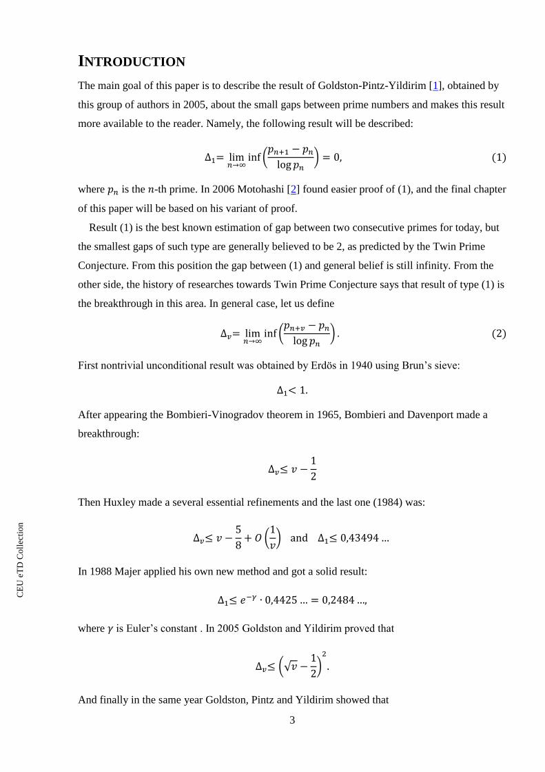
INTRODUCTION

The main goal of this paper is to describe the result of Goldston-Pintz-Yildirim [1], obtained by

this group of authors in 2005, about the small gaps between prime numbers and makes this result

more available to the reader. Namely, the following result will be described:

(

)

where is the -th prime. In 2006 Motohashi [2] found easier proof of (1), and the final chapter

of this paper will be based on his variant of proof.

Result (1) is the best known estimation of gap between two consecutive primes for today, but

the smallest gaps of such type are generally believed to be 2, as predicted by the Twin Prime

Conjecture. From this position the gap between (1) and general belief is still infinity. From the

other side, the history of researches towards Twin Prime Conjecture says that result of type (1) is

the breakthrough in this area. In general case, let us define

(

)

First nontrivial unconditional result was obtained by Erdös in 1940 using Brun’s sieve:

After appearing the Bombieri-Vinogradov theorem in 1965, Bombieri and Davenport made a

breakthrough:

Then Huxley made a several essential refinements and the last one (1984) was:

(

)

In 1988 Majer applied his own new method and got a solid result:

where is Euler’s constant . In 2005 Goldston and Yildirim proved that

(√

)

And finally in the same year Goldston, Pintz and Yildirim showed that

CE

UeT

DC

olle

ctio

n

4

(√ )

The principal idea which made the Goldston-Pintz-Yildirim work is the introduction of

parameter in the Selberg sieve with weight (

)

(see Chapter 6 of this paper).

Appearance of additional parameter plays the crucial role in several estimations in the proof.

Despite the complexity of problem, authors of [1] believe that mathematical society is not so

far to show that

The hypothesis stated in form (3) is called Bounded Gap Conjecture. Belief in inequality (3) has

strong basis. Suppose we have the following inequality:

∑

|

|

Statement which says that for a large with any positive

inequality de (4) holds is called

Bombieri-Vinogradov theorem. Statement which says that in (4) we can have is known as

Elliot-Halberstam Conjecture. Under this conjecture Goldston-Pintz-Yildirim proved in [1] that

This paper has 6 chapters. Chapter 1 is consisted of basic definitions, lemmas and theorems

about the distribution of prime numbers, knowledge of which are required for understanding the

next chapters. The theorems about a logarithmic order of Riemann zeta function in chapter 1 are

necessary for estimations in Chapter 6. Chapters 2, 3, 4 are mainly auxiliary tools for proof of

Bombieri-Vinogradov theorem, but also contain wide applicable and powerful methods.

Chapters 5 and 6 contain complete proofs of Bombieri-Vinogradov and Goldston-Pintz-Yildirim

theorems up to similar cases.

CE

UeT

DC

olle

ctio

n

5

Chapter 1

BASIC TOOLS IN ANALYTIC NUMBER THEORY

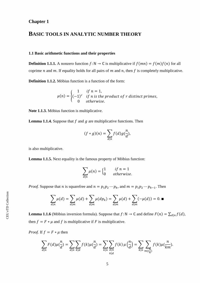
1.1 Basic arithmetic functions and their properties

Definition 1.1.1. A nonzero function is multiplicative if for all

coprime and . If equality holds for all pairs of and , then is completely multiplicative.

Definition 1.1.2. Möbius function is a function of the form:

{

Note 1.1.3. Möbius function is multiplicative.

Lemma 1.1.4. Suppose that and are multiplicative functions. Then

∑

is also multiplicative.

Lemma 1.1.5. Next equality is the famous property of Möbius function:

∑

{

Proof. Suppose that is squarefree and , and . Then

∑

∑

∑

∑

∑

Lemma 1.1.6 (Möbius inversion formula). Suppose that and define ∑

then and is multiplicative if is multiplicative.

Proof. If then

∑

∑∑

∑∑

(

) ∑ ∑

CE

UeT

DC

olle

ctio

n

6

If then sum over is zero, so first claim is proved. Multiplicativity of and Lemma 1.1.4

give us the second claim.

Lemma 1.1.7 (Abel summation formula). Suppose that is continuously differentiable on

and are complex numbers. Then

∑ ∫

Where = ∑

Proof. We can apply the Stieltjes integration by parts on the sum above:

∑

∫

∫

And the result follows.

Corollary 1.1.8. There is a constant such that

∑

Proof. This famous result can be obtained by applying Abel formula with

and

for all .

Definition 1.1.9. The following function is called a von Mangoldt’s function:

{

Note 1.1.10. Von Mangoldt’s function is multiplicative.

Theorem 1.1.11 (Mertens). There is an absolute constant B such that

∑

Proof of this classical result can be found by reader in [3], page 12.

CE

UeT

DC

olle

ctio

n

7

1.2 Dirichlet series and Perron’s formula

Definition 1.2.1. Suppose that are complex numbers and is a complex variable.

Then a series of the form

∑

is called Dirichlet series. The finite sum of the above form is called Dirichlet polynomial.

Lemma 1.2.2. Suppose that and the series ∑ converges. Then the sum

∑ converges uniformly on the compact subsets of the half-plane and the

sum function is holomorphic in that half-plane.

Definition 1.2.3. Abscissa of convergence of the Dirichlet series ∑ is the number

{ ∑

}

Abscissa of absolute convergence of Dirichlet series is called the abscissa of convergence of

∑

Lemma 1.2.4. Suppose that and are complex numbers and the following Dirichlet series

are converge in :

∑

∑

If for , then for all .

Lemma 1.2.5 (Multiplication of Dirichlet series). Suppose that the following Dirichlet series are

converge absolutely in :

∑

∑

Then the Dirichlet series

∑

CE

UeT

DC

olle

ctio

n

8

with ∑ is also absolutely convergent in and .

Proofs of Lemmas 1.2.2, 1.2.4 and 1.2.5 can be found in [3] pp. 14-17.

Lemma 1.2.6 (Perron’s formula). Suppose that . Then

∫

{

This variant of Perron’s formula can be obtained by using the contour integration.

Corollary 1.2.7. Suppose that is the abscissa of absolute convergence of ∑ , and

is not integer. Also let and ∑ . Then

∑

∫

(

∑

| |

)

Proof. Since is not integer, we have

∑ ∑

where is 1, if and is zero, when . Let

then by Lemma 1.2.6:

∑

∑

∫ (

)

(

)

( | (

)| )

∫ ∑

(

∑

| |

)

and Corollary is proved.

1.3 Divisor functions and Euler function.

In this section we consider several standard estimates for divisor function and for sum of

reciprocal Euler functions.

Definition 1.3.1. The divisor function denotes the number of different divisors of integer .

CE

UeT

DC

olle

ctio

n

9

Definition 1.3.2. The generalized divisor function denotes the number of ways, in which

integer can be written as a product of integers.

Note 1.3.3. It is clear that .

Lemma 1.3.4 (Elementary bound for ). For every integer n we have:

√

Proof. Let . If √ then √ , reverse is also true, hence

∑

∑

√

√

Lemma is proved.

Theorem 1.3.5. For and any nonnegative integer we have:

∑

(∑

)

Proof. We will prove it by induction. Case when is trivial. Assume inequality above holds

for . For we can write:

∑

∑

∑

∑

∑( )

∑( )

∑

∑

(∑

)

(∑

)

And result follows.

Theorem 1.3.6. Suppose that is nonnegative integer. Then

∑

(∑

)

Proof. We will prove this theorem by induction again. Case when is clear. Assume that

and do induction for :

CE

UeT

DC

olle

ctio

n

10

∑

∑

∑

∑

∑

By induction hypothesis theorem:

∑

∑

∑

(∑

)

∑

(∑

)

By previous Theorem:

∑

(∑

)

(∑

)

(∑

)

And statement of the Theorem follows.

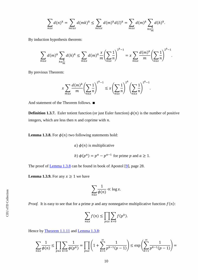
Definition 1.3.7. Euler totient function (or just Euler function) is the number of positive

integers, which are less then and coprime with .

Lemma 1.3.8. For two following statements hold:

is multiplicative

for prime and .

The proof of Lemma 1.3.8 can be found in book of Apostol [9], page 28.

Lemma 1.3.9. For any we have

∑

Proof. It is easy to see that for a prime and any nonnegative multiplicative function

∑

∏ ∑

Hence by Theorem 1.1.11 and Lemma 1.3.8:

∑

∏ ∑

∏( ∑

)

(∑

)

CE

UeT

DC

olle

ctio

n

11

(∑

(∑

))

Proof of Theorem is finished.

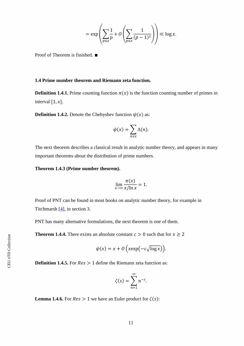
1.4 Prime number theorem and Riemann zeta function.

Definition 1.4.1. Prime counting function is the function counting number of primes in

interval .

Definition 1.4.2. Denote the Chebyshev function as:

∑

The next theorem describes a classical result in analytic number theory, and appears in many

important theorems about the distribution of prime numbers.

Theorem 1.4.3 (Prime number theorem).

Proof of PNT can be found in most books on analytic number theory, for example in

Titchmarsh [4], in section 3.

PNT has many alternative formulations, the next theorem is one of them.

Theorem 1.4.4. There exists an absolute constant such that for

( ( √ ))

Definition 1.4.5. For define the Riemann zeta function as:

∑

Lemma 1.4.6. For we have an Euler product for :

CE

UeT

DC

olle

ctio

n

12

∏(

)

Note 1.4.7. We deduce from Lemma 1.4.6, that doesn’t have zeroes in .

Lemma 1.4.8. For the following equality holds:

∑

Proof. We have

∑

∑

by Lemma 1.1.5 and property of multiplication of Dirichlet series.

Theorem 1.4.9. The function can be analytically continued to a regular function for all

values of , except , where there is a simple pole with residue 1. Extended satisfies the

functional equation:

(

)

Zeroes of in are of special interest in analytic number theory. Existence a

zero-free region of in gives many powerful properties to , so the general

problem in studying such zeroes is an extension of zero-free region to the left of . A part

of original proof of PNT was the next result:

Theorem 1.4.10. There is a constant such that is not a zero for

For .

Theorem 1.4.11. For any and absolute positive constant A the following inequality holds:

|

| ∑

CE

UeT

DC

olle

ctio

n

13

Theorem 1.4.12. uniformly in the region

Theorem 1.4.13 In a region

:

Theorems 1.4.9-1.4.13 reader can find in book of Titchmarsh [4]: Theorem 1.4.9 on p. 13,

Theorem 1.4.10 on p. 54, Theorem 1.4.11 on p. 45, Theorem 1.4.12 on p. 49, Theorem 1.4.13 on

p. 60.

CE

UeT

DC

olle

ctio

n

14

Chapter 2

DIRICHLET CHARACTERS

AND PÓLYA-VINOGRADOV INEQUALITY

2.1 Group characters

Definition 2.1.1. Let G be a finite commutative group of order m. A group homomorphism χ:

→ is called a character of G if for all .

Note 2.1.2. It can be easily established that and that is an -th root of unity:

.

Note 2.1.3. Group characters form a group under pointwise multiplication:

for all . Trivial character is the identity of : for all , and

complex-conjugate character is inverse of .

Theorem 2.1.4. and are isomorphic to each other.

Proof. Suppose that is cyclic with generator . Since every is the -th root of unity,

must be of the form:

for some integer . If then

. We can define

and see that all is generated by , which mean that

is cyclic of order .

Now, let be arbitrary finite abelian group. can be represented as the direct product of cyclic

groups, . Consider . We can define by

for , here is the character in

corresponding to . So, we constructed now an isomorphism between and . Theorem is

proved.

Corollary 2.1.5. Let be an abelian group of finite order and , . Then there is a

character such that .

Proof. Let write as the direct product of cyclic groups, and

. Some is not identity, so let it be . Let be the generator of . Consider the

character corresponding to under the isomorphism from the Theorem 2.1.1. Character

.

CE

UeT

DC

olle

ctio

n

15

Lemma 2.1.6. Let G be a finite abelian group and denote by the trivial character of G. Then

the following two relations hold:

∑

{

∑

{

Proof. Clearly, when is trivial, then (2.1.1) holds. Suppose now that is nontrivial and for

some , . We can write

∑

∑ ∑

∑

Since , the sum on the right side must be equal to 0. Thus (2.1.1) holds.

Clearly, when , then (2.1.2) holds. So, suppose that . There is a by

Corollary 2.1.2. We can write

∑

∑

∑

∑

Again, sum on the right side must be equal to zero. This establishes (2.1.2).

2.2 Dirichlet Characters

Let be an integer. Let be the multiplicative group of . Then is a

cyclic group of order , where is Euler’s function. Let us introduce an extended

function if , where is a character of .

Definition 2.2.1. Extended function denoted above is a Dirichlet character modulo q, or just a

Dirichlet character.

Note 2.2.2. Dirichle characters are not group homomorphisms anymore, but they preserve

multiplicativity: for all . Also we will denote the extension of

trivial group character as principal character modulo q and preserve the notation .

Next lemma is a straightforward consequence of Lemma 2.1.6

Lemma 2.2.3. If is a Dirichlet character modulo q, then

CE

UeT

DC

olle

ctio

n

16

∑

{

∑

{

where the sum on the right side is over all Dirichlet characters modulo q.

Let be a non-principal character modulo , let be a proper divisor of q, and let be a

non-principal character modulo , also let be a principal character modulo q such that

for all (2.2.3)

Definition 2.2.2. We say that induces , if (2.2.3) holds.

Definition 2.2.3. Dirichle character is imprimitive, if we can find and as in (2.2.3),

otherwise is called primitive.

Note 2.2.2. Principal characters are neither primitive, nor imprimitive.

Definition 2.2.4. Let be an imprimitive Dirichlet character modulo q. Conductor of is the

least modulus such that there exists a (necessarily primitive) character modulo , which

induces .

Note 2.2.3. If is primitive, we define its conductor to be equal to the modulus , and if is

principal, we define the conductor to be equal to 1.

2.3 Gaussian Sums

Let is an integer, and is a Dirichlet character modulo . Let us introduce the sum

∑ (

)

Where the summation is over any complete system of residues modulo .

Lemma 2.3.1. Let be a Dirichlet character modulo q and suppose that or is

primitive. Then

. (2.3.2)

CE

UeT

DC

olle

ctio

n

17

Proof. Suppose that If runs through a complete system of residues modulo , then

so does . Then

∑ (

)

∑ (

)

Now, suppose that is primitive and Obviously that = 0. Let ,

. There exists such an integer that , , . Then

∑ (

)

∑ (

)

It follows, that , which establishes the claim of the lemma.

Lemma 2.3.2. Let be a Dirichlet character modulo q and its conductor modulo . Then

(

) (

)

Moreover, if is primitive, then | = √ .

Proof. First, let be primitive. Summing (2.3.2) over all modulo , we get

∑

∑

∑ ∑

∑ (

)

∑ ∑ ∑ (

)

We know that ∑ (

) is the sum of all group characters, corresponding to cyclic

group of order , so it is or 0 according as or not. Hence,

∑

∑

thus, the second claim of lemma holds.

Now turn to general case. Using the properties of möbius function in Lemma 1.1.5, we can

write the principal character modulo as ∑ . Thus,

CE

UeT

DC

olle

ctio

n

18

∑

(

) ∑

(

) ∑

We can change an order of summation in the last sum, so first we will over and then sum

over . But if and

. So, we can replace by or :

∑ ∑ (

)

∑ ∑ (

)

Note that all terms in last sum will be zero if , so we may restrict the summation over

d to the divisors of :

∑ ∑ (

)

Now our aim is to represent as Let write and

. Thus

runs over a complete system of residues modulo

, and runs over a complete system of

residues modulo . We can write

∑ ∑ ∑ (

)

∑ ∑

∑ (

)

Note that ∑ (

) vanishes when

, so and result follows.

2.4 The Pólya - Vinogradov inequality.

Theorem 2.4.1. (Pólya – Vinogradov). Suppose that and are positive integers and is a

non-principal Dirichlet character modulo . Then

| ∑

| √

Proof. First, let be a primitive character. Then, by (2.3.2),

CE

UeT

DC

olle

ctio

n

19

∑

∑ ∑ (

)

∑

∑ (

)

Applying Lemma 2.3.2 we can see that

| ∑

| ∑ | ∑ (

)

|

Modulus of ∑ (

) is equal to:

| ∑ (

)

| |

| |

| |

|

Absolute value of (

) is:

| (

)| √ (

) (

) √ (

) |

|

Similarly we can calculate modulus of (

) . Thus, the inequality (2.4.2) will

transform to

| ∑

| ∑ (

)

Now we apply the inequality for When we can write

∑ (

)

∑ (

)

∑ (

)

∑

∑

∑ (

)

Here we used the fact, that is concave and for all . When

, we have

∑ (

)

∑

∑ (

)

This establishes the theorem for primitive characters.

CE

UeT

DC

olle

ctio

n

20

If is induced by a primitive character modulo , , we have

∑

∑

∑

∑

∑

The sum over m is bounded above by , since is primitive. Thus,

| ∑

| ∑

(

)

where the terms with are equal to 0. If we use that √ from Lemma 1.3.4,

then the result follows.

CE

UeT

DC

olle

ctio

n

21

Chapter 3

AUXILIARY TOOLS IN ANALYTIC NUMBER THEORY

3.1 Some generalized counting functions and primes in arithmetic progressions.

Definition 3.1.1. For a Dirichlet character define

∑ . (3.1.1)

Definition 3.2.2. Define

∑

.

Lemma 3.1.1. Suppose that is a character modulo induced by a primitive character

modulo . Also let be a principal character modulo . Then following three

relations hold:

. (3.1.2)

√ (3.1.3)

∑ (3.1.4)

Proof. First we will prove (3.1.2). We have

∑

∑

∑

which establishes (3.1.2). Using the Theorem 1.4.4 and (3.1.2) we can write for

√

which proves (3.1.3). For right part of (3.1.4) we have

∑

∑ ∑

∑ ∑

If denote the as inverse of modulo , and of we write as , then and

and the right part of last equality will be

equal to

CE

UeT

DC

olle

ctio

n

22

∑ ∑

∑

and the result follows.

Theorem 3.1.2 (Siegel-Walfisz). Let be a real fixed constant and where

. Then exists a positive constant depending only on such that

( √ )

Theorem 3.1.2 describes the asymptotic law of distribution of prime numbers in arithmetic

progressions with best known error term. More about Siegel-Walfisz theorem can be found in

book [5] of Davenport.

3.2 Vaughan Identity

Theorem 3.2.1 (Vaughan). Suppose that Then

∑

where

∑ ∑

∑ ∑

∑ ∑

with coefficients and

Proof. Let us write a trivial identity

(3.2.2)

We can choose and to be arbitrary functions, in particular Dirichlet polynomials:

∑ and ∑ .

Our task is to compare the coefficients of in the Dirichlet series representations of the left

and right sides of (3.2.2) to obtain an identity for . We have

CE

UeT

DC

olle

ctio

n

23

∑

∑

∑

∑

∑

∑

∑

(∑

∑

) ( )

∑

∑

∑

( )

From Lemmas 1.4.8 and 1.1.5

∑ and ∑ when .

Last summand from (3.2.2) can be written as

∑

∑

∑

∑

∑

∑

∑

∑

∑

So, for we obtain the following identity for :

∑

∑

∑

∑

Multiplying both sides by and summing over we obtain Vaughan identity with

∑

∑

And, easy to see that ∑ and

Vaughan identity was found by Vaughan in 1977, and can be used for decomposing sums over

primes into double sums, which are easier to evaluate. One of the applications of the Vaughan

identity is simplification of proof of Bombieri-Vinogradov’s theorem; it will be demonstrated in

Chapter 5 of this paper.

CE

UeT

DC

olle

ctio

n

24

Chapter 4

ONE RESULT FROM THE LARGE SIEVE

4.1 Inequality, which is involving an exponential sum

Theorem 4.1.1 Suppose that – arbitrary complex numbers and

∑

Moreover, let be – arbitrary real numbers and ‖ ‖ where operator

‖ ‖ means distance to the closest integer. Then

∑

∑

Proof. Let be an arbitrary real number, such that (

) – real number, such that

and

∑

- arbitrary Fourier series, which contains only cosines, and for which series ∑ converges, and

function when ‖ ‖ . Also suppose, that when Denote

∑

Then is convolution of functions and , it means

∫

∫

After applying the Cauchy inequality we have

CE

UeT

DC

olle

ctio

n

25

( ∫( )

)( ∫

) (∫( )

)( ∫

)

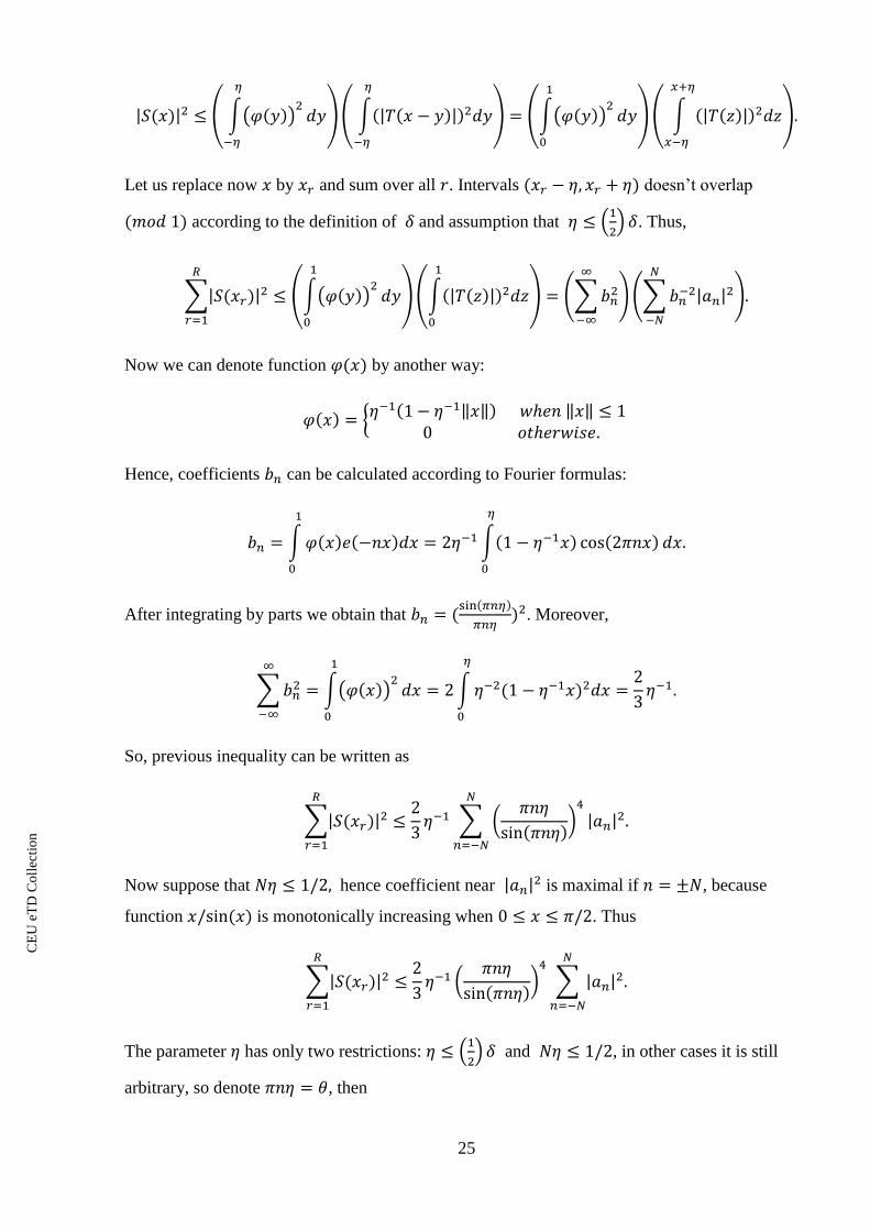
Let us replace now by and sum over all . Intervals doesn’t overlap

according to the definition of and assumption that (

) . Thus,

∑

(∫( )

)(∫

) (∑

)(∑

)

Now we can denote function by another way:

{ ‖ ‖ ‖ ‖

Hence, coefficients can be calculated according to Fourier formulas:

∫

∫

After integrating by parts we obtain that

. Moreover,

∑

∫( )

∫

So, previous inequality can be written as

∑

∑ (

)

Now suppose that hence coefficient near is maximal if , because

function is monotonically increasing when . Thus

∑

(

)

∑

The parameter has only two restrictions: (

) and , in other cases it is still

arbitrary, so denote , then

CE

UeT

DC

olle

ctio

n

26

(

)

Where is arbitrary number, satisfying two conditions (

) and

Function is decreasing, when is increasing from 0 to , where is the

unique solution of equation

, such that . If (

) then

denote . Then

If (

) , then denote (

) , in this case

After calculations we find that , it means that

Theorem is proved.

Lemma 4.1.2 Suppose that and are positive integers. Then

∑ ∑ | ∑

|

∑

Proof. First we will replace variable of summation to , where is running between

integers and . Denote (

) or (

) if is even or odd, and

So, now is running between and or , in the last case we can create extra

zero coefficient.

Now we can apply Theorem 4.1.1. Numbers in this theorem will be rational

numbers , for which the smallest of possible denominators Now, if and

we have

‖

‖

Hence, and lemma is proved.

CE

UeT

DC

olle

ctio

n

27

4.2 Main lemma

Lemma 4.2.1. Suppose that are positive integers. Then

∑

∑ | ∑

|

∑

Where denotes a summation restricted to primitive characters.

Proof. When is primitive, from Lemmas 2.3.1 and 2.3.2 we can deduce that

| ∑

|

| ∑

|

|| ∑

||

Where ∑ Hence

∑ | ∑

|

∑ || ∑ (

)

||

∑

∑

∑ | (

)|

Where denotes the multiplicative inverse of modulo q. Thus, the result follows after

applying the Lemma 4.1.2.

Lemma 4.2.1 plays an important role in estimating sums in Bombieri-Vinogradov theorem.

More about large sieve reader can find in book of Davenport [5], p.151 and in Russian version of

this book [6], p.147.

CE

UeT

DC

olle

ctio

n

28

Chapter 5

BOMBIERI-VINOGRADOV THEOREM

5.1 Main theorem

Bombieri-Vinogradov theorem is extremely important result in analytic number theory, which

was proved in 1965, and has various applications. Sometimes it is called just Bombieri theorem.

Theorem 5.1.1 (Bombieri-Vinogradov). Suppose that is real number and Then

for any fixed real number ,

∑

|

|

Proof. First define

{

By (3.1.4),

∑

( )

hence

|

|

∑ | |

Writing for the left side of (5.1.1), we find that

∑

∑

| |

where denotes the contribution from the principal characters and from all other characters.

Lemma 1.3.9 says that

∑

By (3.1.3) and (5.1.2) we have

CE

UeT

DC

olle

ctio

n

29

( √ ) ∑

Where is the absolute constant. Let be the primitive character inducing modulo . By

(3.1.2),

∑

∑

Let . Then we can estimate the sum over the characters by double sum, where the

summation in first sum will be over all , and summation in second will be over all

primitive characters modulo . We have

∑ ∑

∑

∑

∑

where we have used (5.1.2) again. Now, our idea is to estimate the contribution from the “small”

moduli . For this we can represent in (3.1.4) as in Siegel-Walfisz theorem and

as in (3.1.3) for principal characters. We have

( √ )

For all primitive characters to moduli , say. Hence

∑

∑

( √ )

Combining this estimation and (5.1.3), we obtain

where

∑

∑

CE

UeT

DC

olle

ctio

n

30

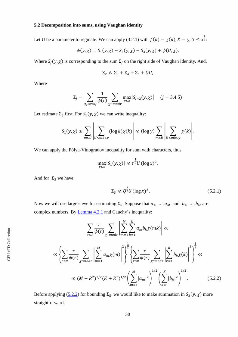
5.2 Decomposition into sums, using Vaughan identity

Let U be a parameter to regulate. We can apply (3.2.1) with

Where is corresponding to the sum on the right side of Vaughan Identity. And,

Where

∑

∑

| |

Let estimate first. For we can write inequality:

∑ | ∑

|

∑ | ∑

|

We can apply the Pólya-Vinogradov inequality for sum with characters, thus

And for we have:

Now we will use large sieve for estimating . Suppose that and are

complex numbers. By Lemma 4.2.1 and Cauchy’s inequality:

∑

∑ |∑ ∑

|

{∑

∑ |∑

|

}

{∑

∑ |∑

|

}

(∑

)

(∑

)

Before applying (5.2.2) for bounding we would like to make summation in more

straightforward.

CE

UeT

DC

olle

ctio

n

31

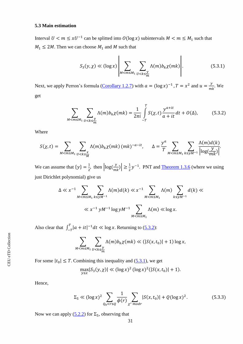
5.3 Main estimation

Interval can be splitted into subintervals such that

Then we can choose and such that

| ∑ ∑

|

Next, we apply Perron’s formula (Corollary 1.2.7) with and

. We

get

∑ ∑

∫

Where

∑ ∑

∑ ∑

|

|

We can assume that { }

then |

|

PNT and Theorem 1.3.6 (where we using

just Dirichlet polynomial) give us

∑ ∑

∑ ∑

∑

Also clear that ∫

. Returning to (5.3.2):

∑ ∑

For some Combining this inequality and (5.3.1), we get

Hence,

∑

∑

Now we can apply (5.2.2) for , observing that

CE

UeT

DC

olle

ctio

n

32

∑

∑

∑

because of PNT and

∑

∑

because of Theorem 1.3.6. Hence (5.2.2) yields

∑

∑

(

)

From this inequality and (5.3.3) a new inequality can be derived for by using a dyadic

decomposition:

(

)

5.4 Completion of the proof

We can still regulate parameter now let

. Then we can decompose on

two smaller sums, where in first sum and in the second

∑ ∑

∑ ∑

say.

We can estimate right now:

∑ | ∑

|

So , clearly can be bounded similarly to , and

similarly to ,

hence the contribution of

to can be estimated similarly to and to

respectively. Omitting all calculations, we can write for

(

)

So finally can be estimated. For this we need to combine all bounds for , we get

(

)

We can see that to satisfy the condition of theorem the next two inequalities must hold:

CE

UeT

DC

olle

ctio

n

33

Thus

and for which theorem is proved. Now

suppose that . Consider the trivial bound for :

∑

|

|

∑

∑

which is better, then bound in the theorem for such . Bombieri-Vinogradov theorem is

proved.

Proof of Bombieri-Vinogradov theorem introduced here is based on proof in [3], pp. 77-81.

Alternative proof can be found in book of Huxley [7], pp.103-107

CE

UeT

DC

olle

ctio

n

34

Chapter 6

GOLDSTON-YILDIRIM-PINTZ THEOREM

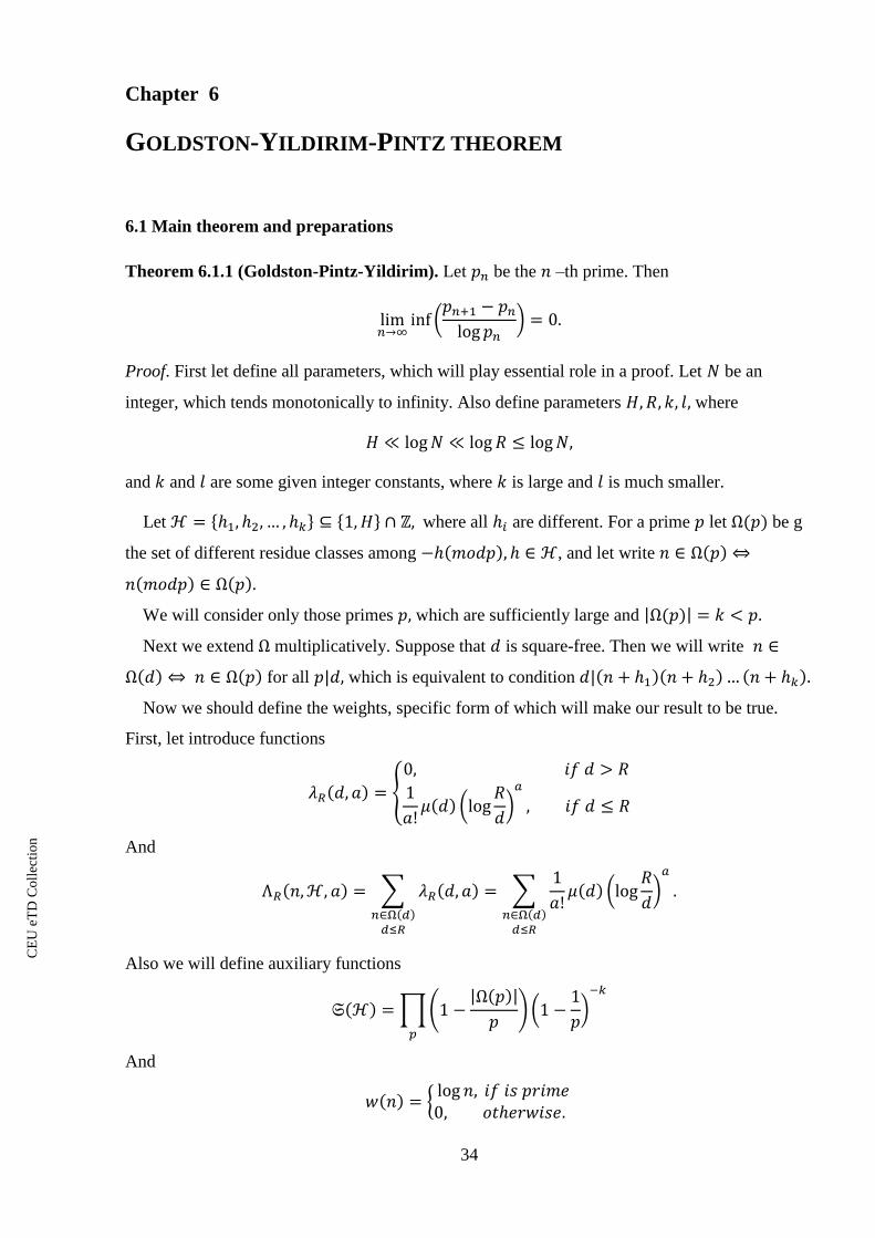
6.1 Main theorem and preparations

Theorem 6.1.1 (Goldston-Pintz-Yildirim). Let be the –th prime. Then

(

)

Proof. First let define all parameters, which will play essential role in a proof. Let be an

integer, which tends monotonically to infinity. Also define parameters where

and and are some given integer constants, where is large and is much smaller.

Let { } { } where all are different. For a prime let be g

the set of different residue classes among , and let write

We will consider only those primes which are sufficiently large and

Next we extend multiplicatively. Suppose that is square-free. Then we will write

for all which is equivalent to condition

Now we should define the weights, specific form of which will make our result to be true.

First, let introduce functions

{

(

)

And

∑

∑

(

)

Also we will define auxiliary functions

∏(

)

(

)

And

{

CE

UeT

DC

olle

ctio

n

35

Our main goal is to show that

∑ ∑ (∑

)

is positive. When it is true then exists such that

∑

That means that there exist two primes such that If we

will show that we can make where is an arbitrary small number, then theorem

will be proved. Positivity of sum in (6.1.1) follows from next three lemmas:

Lemma 1. Assume that

with some large depending on Then

∑

(

)

Denote an error term above as .

Lemma 2. Assume, in addition to the above, that also where is a parameter below

Then

∑

{

{ }

(

)

(

)

Lemma 3 (Gallagher 1976). Suppose that Then

∑

( )

where summation is over all ordered subsets of of length .

Now we will combine all of this Lemmas to estimate sum in (6.1.1). Thus

∑ ∑ ∑

∑ ∑

CE

UeT

DC

olle

ctio

n

36

∑ ∑ ∑

∑ ∑ ∑

∑ ∑

∑ ∑ { }

(

)

∑ ∑

(

)

∑

(

)

(

)

(

)

(

)

(

) (

)

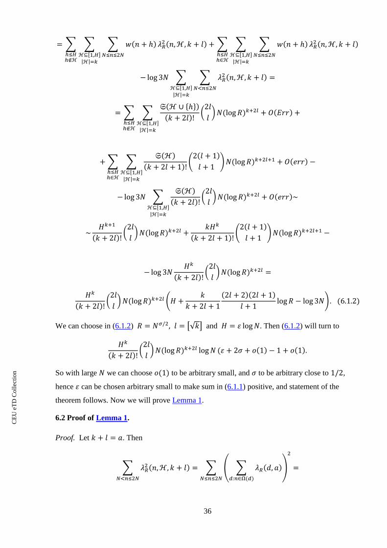
We can choose in (6.1.2) [√ ] and . Then (6.1.2) will turn to

(

)

So with large we can choose to be arbitrary small, and to be arbitrary close to ,

hence can be chosen arbitrary small to make sum in (6.1.1) positive, and statement of the

theorem follows. Now we will prove Lemma 1.

6.2 Proof of Lemma 1.

Proof. Let . Then

∑

∑ ( ∑

)

CE

UeT

DC

olle

ctio

n

37

∑

∑

∑

∑

( ( ))

∑

| ( ( ))|(

( ) )

∑

| ( ( ))|

( )

(∑

| ( ( ))|)

Since | ( ( ))| and , and Theorem 1.3.6 the error

term in the sum above can be written as:

(∑

| ( ( ))|) ∑

Define ( ). Then the sum in Lemma 1 is , where

∑

We can write

∫ (

)

, so for we have:

∫ ∫ ( ∑

)

Define ∑

. Using properties of Riemann zeta function and

multiplicativity of and we can write the Euler product for

∏(

(

))

Also define our main auxiliary function in this proof:

(

)

CE

UeT

DC

olle

ctio

n

38

The Euler product for is:

∏(

)(

)

(

)

(

)

We assumed earlier that hence the logarithm of the corresponding Euler factor is

(

) (

) (

)

(

)

This logarithmic factor is equal to . Hence for

and the

sum of this logarithms converge absolutely, i.e. is holomorphic in this region.

Moreover, we will note that . For bounding we will estimate its

logarithmic sum:

∑ ( (

) (

) (

)

(

)) ∑

∑

Where

and ∑

by Merten’s theorem

1.1.11.

Hence . So, again consider the T as

∫ ∫ ( (

)

)

Now shift a contour from to

and from to

, where

√ . Also we truncate - integral to and - integral to

, and denote the results by and respectively. We didn’t obtain any new poles while

shifting, so we only need to calculate truncated parts. Thus

By Theorem 1.4.11 we have

√

CE

UeT

DC

olle

ctio

n

39

√ √

(

) (

√ ) (√ )

Combining (6.2.1)-(6.2.4) we have

|( (

)

) | ( √ )

For some constant . So, we can write for truncated error:

∬ ( (

)

)

( √ ) ∬

( √ ) ∫

( √ )

for a sufficiently large . Now let fix and shift a contour from

to

and denote the result by . For calculating the error after shifting, we should admit that

is still holomorphic at the hence bounded,

are the powers of by Theorem 1.4.12, term is also bounded here, and

makes an error small:

√ (

√ ) ( √ )

where is a positive constant. Similarly to the previous calculations the new error will be of

( √ ). Denoting

( (

)

)

as and applying (6.2.6) and (6.2.7) we can write for :

∫( ( )

)

( √ )

First, let calculate . For this we will create a circle with center in

with sufficiently small radius. Then on :

CE

UeT

DC

olle

ctio

n

40

√

√

So

√ . Hence

Also on

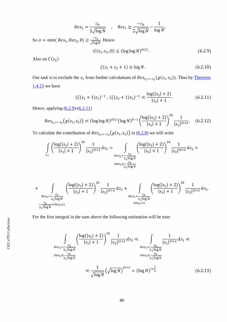
Our task is to exclude the from further calculations of . Thus by Theorem

1.4.13 we have

Hence, applying (6.2.9)-(6.2.11)

( ) (

)

To calculate the contribution of ( ) in (6.2.8) we will write

∫ (

)

∫ (

)

√

√

∫ (

)

√

√

∫ (

)

√

For the first integral in the sum above the following estimation will be true:

∫ (

)

√

√

∫

√

√

√ (√ )

CE

UeT

DC

olle

ctio

n

41

For the second integral we have:

∫ (

)

√

√

∫

√

√

∫

√

(√ )

And the third integral can be bounded in the following way:

∫ (

)

√

∫

Combining (6.2.8) and (6.2.12)-(6.2.15) we have

∫ ( )

We will call the following function:

(

)

Note, that is holomorphic around and . Now shift

the integration contour from {

} to {

}.

This way we get

∫ ∫

where is the positive small constant and error from shifting the contour can be calculated in

similar way to (6.2.7), and is of order ( ( √ )) Let change the variables in double

integral above: Then

∫ ∫

CE

UeT

DC

olle

ctio

n

42

∫ ∫

∫

∫

To calculate the pole of (

) we need to know the coefficient near of

Teylor series of in neighborhood of zero, which has value

∑ , where . Substituting this value

into (6.2.17) we get

∫

∫

∫

∫

We observe that

∑ ( )

, hence the pole of this function and integral in

(6.2.18) will be equal to ( ). Hence

(

)

Remembering that the sum in Lemma 1 is , we finishing proof of Lemma 1.

6.3 Proof of Lemma 2.

Proof. We should make remark, that the sum in Lemma 2 doesn’t change if we replace by

{ } This is because if is not a zero then is prime and

∑

(

)

CE

UeT

DC

olle

ctio

n

43

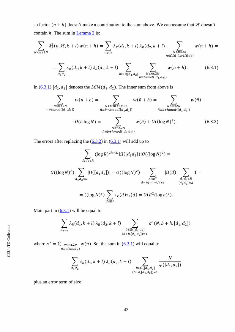
so factor doesn’t make a contribution to the sum above. We can assume that doesn’t

contain . The sum in Lemma 2 is:

∑

∑

∑

∑

∑ ∑

In (6.3.1) denotes the . The inner sum from above is

∑

∑

∑

∑

The errors after replacing the (6.3.2) in (6.3.1) will add up to

∑

∑

∑

∑

∑

Main part in (6.3.1) will be equal to

∑

∑

where ∑

. So, the sum in (6.3.1) will equal to

∑

∑

plus an error term of size

CE

UeT

DC

olle

ctio

n

44

∑

∑ |

|

∑

∑ |

|

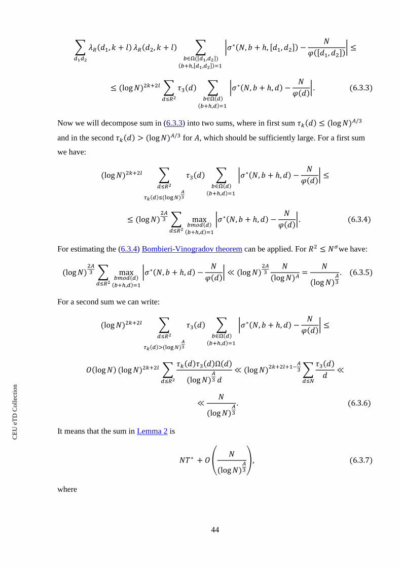
Now we will decompose sum in (6.3.3) into two sums, where in first sum

and in the second for , which should be sufficiently large. For a first sum

we have:

∑

∑ |

|

∑

|

|

For estimating the (6.3.4) Bombieri-Vinogradov theorem can be applied. For we have:

∑

|

|

For a second sum we can write:

∑

∑ |

|

∑

∑

It means that the sum in Lemma 2 is

(

)

where

CE

UeT

DC

olle

ctio

n

45

∑

∑

The innermost sum is by Chinese theorem:

∑

∏ ∑

∏

where is the cardinality of the set { }. As before

We can calculate similarly to in Lemma 1 and will have a following form:

∫ ∫ ∏(

(

))

Omitting the calculations we can write for , when :

{ }

(

)

And when :

(

)

Substituting the expression of into (6.3.7) we will obtain the result of Lemma 2.

This chapter is based on paper of Motohashi [2], who found easier proof in 2006, then the

original proof of Goldston-Pintz-Yildirim, which reader can find in [1]. Proof of Gallagher

Lemma can be found in [8].

CE

UeT

DC

olle

ctio

n

46

CONCLUSION

In this work we introduced the complete proof of Goldston-Pintz-Yildirim theorem – the best

known result on estimating the small gaps between consecutive primes. Also various wide

applicable inequalities were highlighted, such as Bombieri-Vinogradov theorem, Pólya-

Vinogradov inequality, large sieve method for character sums. Correlation and utility of analytic

tools were presented – we showed the Vaughan identity as a simplifier in Bombieri-Vinogradov

theorem’s proof, and Bombieri-Vinogradov result as crucial part of Goldston-Pintz-Yildirim

theorem.

The flexibility and variety of tools in analytic number theory demonstrate us, that many areas in

prime number theory experience rapid development, and breakthrough is possible not only in

bounding the small gaps between primes, but also in estimating the number of primes in short

intervals, in Goldbach conjecture and other topics related to distribution of primes.

CE

UeT

DC

olle

ctio

n

47

REFERENCES

[1] D.A. Goldston, J. Pintz, C.Yildirim, Primes in tuples (2009),

http://www.math.sjsu.edu/~goldston/Tuples1.pdf.

[2] D.A. Goldston, Y. Motohashi, J. Pintz, C.Y. Yildirim, Small gaps between primes exist,

Proc. Japan Acad. 82A (2006), 61-65.

[3] A. Kumchev, The Distribution of prime numbers, (2005),

http://pages.towson.edu/akumchev/DistributionOfPrimesNotes.pdf.

[4] E.C. Titchmarsh, The theory of the Riemann zeta-function, Clarendon Press, Oxford

(1951).

[5] H. Davenport, Multiplicative number theory, Second edition, Springer-Verlag, New-York,

(1967).

[6] H. Davenport, Multiplikativnaja teorija chisel (Russian), Izdatelsvo “Nauka”, Moskva,

(1971).

[7] M. N. Huxley, The distribution of prime numbers, Clarendon Press, Oxford, (1972).

[8] P. X. Gallagher, On the distribution of primes in short intervals, Mathematika 23 (1976),

no.1, 4-9.

[9] T.M. Apostol, Introduction to analytic number theory, Springer-Verlag, New-York,

(1976).