Supervision of Discrete Event Systems Based on...

UNIVERSIDADE DE LISBOA

INSTITUTO SUPERIOR TECNICO

Supervision of Discrete Event SystemsBased on Temporal Logic Specifications

Bruno Filipe Araujo de Lacerda

Supervisor: Doctor Pedro Manuel Urbano de Almeida Lima

Thesis approved in public session to obtain the PhD Degree in

Electrical and Computer Engineering

Jury Final Classification: Pass with Merit

Jury

Chairperson: Chairman of the IST Scientific Board

Members of the Committee:

Doctor Alessandro Giua

Doctor Jorge Manuel Miranda Dias

Doctor Pedro Manuel Urbano de Almeida Lima

Doctor Paulo Alexandre Carreira Mateus

Doctor Paulo Jorge Coelho Ramalho Oliveira

2013

UNIVERSIDADE DE LISBOA

INSTITUTO SUPERIOR TECNICO

Supervision of Discrete Event SystemsBased on Temporal Logic Specifications

Bruno Filipe Araujo de Lacerda

Supervisor: Doctor Pedro Manuel Urbano de Almeida Lima

Thesis approved in public session to obtain the PhD Degree in

Electrical and Computer Engineering

Jury Final Classification: Pass with Merit

Jury

Chairperson: Chairman of the IST Scientific Board

Members of the Committee:

Doctor Alessandro Giua, Full Professor, University of Cagliari, Italy;

Doctor Jorge Manuel Miranda Dias, Professor Associado (com Agregacao) da Faculdade

de Ciencias e Tecnologia, da Universidade de Coimbra;

Doctor Pedro Manuel Urbano de Almeida Lima, Professor Associado (com Agregacao)

do Instituto Superior Tecnico, da Universidade de Lisboa;

Doctor Paulo Alexandre Carreira Mateus, Professor Associado (com Agregacao) do

Instituto Superior Tecnico, da Universidade de Lisboa;

Doctor Paulo Jorge Coelho Ramalho Oliveira, Professor Associado do Instituto Superior

Tecnico, da Universidade de Lisboa.

Funding InstitutionsFundacao para a Ciencia e a Tecnologia through grant FRH/BD/45046/2008; Fundacao para a Ciencia e

a Tecnologia (ISR/IST pluriannual funding) through the PIDDAC Program funds.

2013

Abstract

In this work, a methodology for performing supervisory control of discrete event systems based on

linear temporal logic is presented. The discrete event system is modelled as a finite state automaton

or a Petri net and, given a linear temporal logic safety specification written over the events and the

states of the system, either a finite state automaton or a Petri net that realizes a supervisor that restricts

the behaviour of the system so that it satisfies the specification is constructed. The first step of the

methodology is based on defining semantics for evaluating the linear temporal logic formulas in both

the finite state automaton and the Petri net models. These semantics are then used to compose the

corresponding model with the Buchi automaton representing the linear temporal logic formula. The

result of each composition is the minimal restriction of the uncontrolled behaviour that satisfies the

formula. A strictly symbolic semantics is defined for both finite state automata and Petri nets, and a

more general semantics for Petri nets that includes and takes advantage of the fact that in Petri nets

the state can be described algebraically is also introduced. This generalized semantics also has the

benefit of reducing the size of the supervisor realizations, when compared to the strictly symbolic ap-

proach. The structure obtained from the presented compositions represents a coarse realization for the

supervisor, for which one can apply existing approaches in the literature to verify and enforce relevant

properties in supervisory control theory, such as admissibility and deadlock-freeness. A discussion

on how to apply these approaches for the results of the compositions presented in this work is also

provided. For the case of Petri nets, the inherent limitations of the model with regards to supervisory

control theory are also addressed. To illustrate and compare the models and semantics used in the

methodology, three examples of application are described: a social robot, a team of simulated soccer

robots and a real multi-robot surveillance scenario mock-up.

i

Keywords: Discrete Event Systems, Supervisory Control, Finite State Automata, Petri Nets, Lin-

ear Temporal Logic, Formal Methods, Task Specification, Robotics, Multi-Robot Coordination, Mul-

tiagent Systems

ii

Resumo

Neste trabalho apresenta-se uma metodologia para realizar controlo por supervisao de sistemas de

eventos discretos, baseada em logica temporal linear. O sistema de eventos discretos e modelado

como um automato de estados finito ou uma rede de Petri e, dada uma especificacao de seguranca

em logica temporal linear escrita sobre os eventos e estados do sistema, e construıdo respectivamente

um automato de estados finito ou uma rede de Petri. Esta nova estrutura realiza um supervisor que

restringe o comportamento do sistema, tal que este satisfaca a especificacao. O primeiro passo da

metodologia baseia-se em definir semanticas para avaliar as formulas de logica temporal linear nos

modelos automato de estados finito e rede de Petri. Estas semanticas sao entao utilizada para compor

o modelo correspondente com o automato de Buchi que representa a formula. O resultado de cada

composicao representa a menor restricao do comportamento nao-controlado que satisfaz a formula.

Uma semantica estritamente simbolica e definida tanto para automatos de estados finitos como para

redes de Petri, e e tambem introduzida uma semantica mais geral para redes de Petri, que inclui e tira

proveito do facto do estado de uma rede de Petri poder ser descrito algebricamente. Esta semantica

generalizada apresenta tambem o benefıcio de reduzir o tamanho das realizacoes de supervisores,

quando comparada com a abordagem estritamente simbolica. A estrutura obtida pelas composicoes

apresentadas representa uma realizacao grosseira para o supervisor, para a qual se podem aplicar

abordagens existentes na literatura para verificar e fazer cumprir propriedades relevantes para a teoria

de controlo por supervisao, tais como admissibilidade e liberdade de deadlocks. Uma discussao focada

na aplicacao destas abordagens para os resultados das composicoes apresentadas neste trabalho e

tambem fornecida. Para o caso das redes de Petri, as limitacoes inerentes do modelo em relacao a

teoria de controlo por supervisao sao tambem abordadas. Com o objectivo de ilustar e comparar os

modelos e semanticas utilizados na metodologia, tres exemplos de aplicacao sao descritos: um robot

social, uma equipa de robots futebolistas simulados e um cenario real de vigilancia multi-robot.

iii

Palavras-Chave: Sistemas de Eventos Discretos, Controlo por Supervisao, Automatos de Estados

Finito, Redes de Petri, Logica Temporal Linear, Metodos Formais, Especificacao de Tarefas,

Robotica, Coordenacao Multi-Robot, Sistemas Multi-Agente

iv

AcknowledgementsThe sun is setting in Lisbon – as usual, I’m finishing writing later than expected – and I’m in 6.15

writing the last few words of my thesis. Finally, I’ve got this done and, though the feelings are mixed,

one of them is of fulfilment: After more than 4 years I finally have my work ready to be handed in

for evaluation! This could not have been done without the help of many people and I’d like to thank

some of them.

First and foremost, I’d like to thank my advisor, Prof. Pedro Lima. His impact on my academic

life has been immeasurable, starting in 2006 when he accepted to supervise my Master’s thesis (during

which I realized that research life might not be that bad), being available to taking me back for a short-

time grant when, after 6 months of consulting work, I decided that I’d like to return to academia and

see if continuing for a PhD was something that I wanted and, finally, for his guidance and patience

throughout my PhD studentship. I would also like to thank Profs. Alessandro Saffiotti, Miguel Salichs

and Paulo Tabuada for receiving me, for 3 months each, in their respective research groups. All of

these stays were very learning and enjoyable experiences.

I also want to thank my colleagues, mainly all the guys in 6.15 for putting up with me all this time,

and the guys in 6.12 for putting up with my e-puck scenario in the middle of their room (and also me,

once in a while). I’m leaving ISR for now, but you will be missed and I hope we can see each other

soon.

To my friends, both the Lisbon people and the Faial people (some of them waiting for me for

dinner right now), your constant presence and support was fundamental for me. It would have been

impossible to finish this work without having people that I like in the “outside world”, always available

to hang out and do stuff. I will not name you all, but if you’re taking your time to read these words

you’re very probably one of them, so thank you!

Finally, I’d like to thank my family for all their support throughout all these years, and all the

sacrifices that I know were made so I could come to Lisbon to study. Unfortunately, one of the results

of those sacrifices was me following a path where I cannot be near you, but you are missed everyday.

And with this, the sun is down. Time to print this thing and get out of here.

v

Contents

Abstract i

Resumo iii

1 Introduction 11.1 Overview . . . . . . . . . . . . . . . . . . . . . . . . . . . . . . . . . . . . . . . . 1

1.2 Related Work . . . . . . . . . . . . . . . . . . . . . . . . . . . . . . . . . . . . . . 3

1.3 Thesis Goals and Contributions . . . . . . . . . . . . . . . . . . . . . . . . . . . . . 10

1.4 Document Organization . . . . . . . . . . . . . . . . . . . . . . . . . . . . . . . . . 10

2 System Modelling 132.1 Finite State Automata . . . . . . . . . . . . . . . . . . . . . . . . . . . . . . . . . . 13

2.2 Petri Nets . . . . . . . . . . . . . . . . . . . . . . . . . . . . . . . . . . . . . . . . 17

2.2.1 Symbolic State Description . . . . . . . . . . . . . . . . . . . . . . . . . . 25

2.2.2 Linear Algebraic State Description . . . . . . . . . . . . . . . . . . . . . . . 31

3 Specification Language 413.1 Linear Temporal Logic . . . . . . . . . . . . . . . . . . . . . . . . . . . . . . . . . 41

3.1.1 Syntax and Semantics over the System Models . . . . . . . . . . . . . . . . 41

3.1.2 Translation to Buchi automata . . . . . . . . . . . . . . . . . . . . . . . . . 45

3.2 Restricting LTL to Safety Properties . . . . . . . . . . . . . . . . . . . . . . . . . . 49

4 Composition of Buchi Automaton with System Models 534.1 Finite State Automata . . . . . . . . . . . . . . . . . . . . . . . . . . . . . . . . . . 54

4.2 Petri Nets . . . . . . . . . . . . . . . . . . . . . . . . . . . . . . . . . . . . . . . . 56

4.2.1 Adding Minimal Satisfying Transitions . . . . . . . . . . . . . . . . . . . . 57

4.2.2 Composition Algorithm . . . . . . . . . . . . . . . . . . . . . . . . . . . . 81

4.3 Concluding Remarks . . . . . . . . . . . . . . . . . . . . . . . . . . . . . . . . . . 91

5 Supervisor Realization 935.1 Supervisory Control Basics . . . . . . . . . . . . . . . . . . . . . . . . . . . . . . . 93

5.2 Dealing with Admissibility and Deadlock-Freeness . . . . . . . . . . . . . . . . . . 99

vii

5.2.1 Finite State Automata . . . . . . . . . . . . . . . . . . . . . . . . . . . . . 99

5.2.2 Petri Nets . . . . . . . . . . . . . . . . . . . . . . . . . . . . . . . . . . . . 101

5.3 Specification Language Restriction for Admissibility . . . . . . . . . . . . . . . . . 115

5.4 Decentralized Approach . . . . . . . . . . . . . . . . . . . . . . . . . . . . . . . . 120

5.5 Generalized Mutual Exclusion Constraints . . . . . . . . . . . . . . . . . . . . . . . 126

6 Case Studies and Results 1296.1 Simulated Soccer Robots . . . . . . . . . . . . . . . . . . . . . . . . . . . . . . . . 130

6.2 Maggie, The Social Robot . . . . . . . . . . . . . . . . . . . . . . . . . . . . . . . 137

6.3 Surveillance Scenario with E-Pucks . . . . . . . . . . . . . . . . . . . . . . . . . . 142

6.3.1 Scenario Description . . . . . . . . . . . . . . . . . . . . . . . . . . . . . . 142

6.3.2 PN Models and LTL Specifications . . . . . . . . . . . . . . . . . . . . . . 145

7 Conclusions and Further Work 1497.1 Conclusions . . . . . . . . . . . . . . . . . . . . . . . . . . . . . . . . . . . . . . . 149

7.2 Further work . . . . . . . . . . . . . . . . . . . . . . . . . . . . . . . . . . . . . . 150

Appendices 155

A PN Models for the Surveillance Scenario 157

viii

List of Figures

1.1 The proposed methodology (for PN models and supervisors), with the several steps

of the algorithm depicted with dashed arrows and the feedback loop of supervisory

control depicted with solid arrows. (a) A Petri net system model G. (b) The feedback

loop of supervisory control (with a PN realizing the supervisor). (c) An LTL formula

ϕ . (d) Buchi automaton Bϕ accepting exactly the infinite sequences that satisfy ϕ .

(e) A fragment of the supervisor Sϕ that restricts the behaviour of G to the largest

sub-behaviour which is consistent with ϕ . . . . . . . . . . . . . . . . . . . . . . . . 4

2.1 FSA System Model for Robot with a Light Actuator . . . . . . . . . . . . . . . . . . 15

2.2 FSA System Model for a Robot with a Sound Actuator . . . . . . . . . . . . . . . . 16

2.3 FSA System Model for a Robot with a Light and Sound Actuator . . . . . . . . . . . 16

2.4 Illustration of a complement place. . . . . . . . . . . . . . . . . . . . . . . . . . . . 22

2.5 Illustration of the complement place construction. . . . . . . . . . . . . . . . . . . . 23

2.6 PN system model with symbolic state description for a tea/coffee machine . . . . . . 27

2.7 PN model for robot 1 . . . . . . . . . . . . . . . . . . . . . . . . . . . . . . . . . . 31

2.8 PN model for robot 2 . . . . . . . . . . . . . . . . . . . . . . . . . . . . . . . . . . 32

2.9 PN representing the composition of 2.7 and 2.8 . . . . . . . . . . . . . . . . . . . . 32

2.10 PN system model with algebraic state description for a tea/coffee machine . . . . . . 34

2.11 Petri net model of a card player . . . . . . . . . . . . . . . . . . . . . . . . . . . . . 38

2.12 Petri net model of the complete card playing game . . . . . . . . . . . . . . . . . . 39

3.1 BA obtained from G(start moving⇒ (X(¬stop movingUgoal reached))) . . . . . . 48

3.2 BA accepting L = {σ ∈ (2Π)ω | π ∈ σ2i, i ∈ N} . . . . . . . . . . . . . . . . . . . . 48

3.3 Non-deterministic BA accepting the ω-language generated by (FGπ). . . . . . . . . 49

3.4 Deterministic BA accepting the language generated by (Fπ). . . . . . . . . . . . . . 50

3.5 Venn diagram for the classes of ω-languages described in this chapter. . . . . . . . . 52

4.1 (a) A fragment of an FSA system model (b) A fragment of a BA . . . . . . . . . . 56

4.2 A fragment of the obtained FSA system model . . . . . . . . . . . . . . . . . . . . . 56

4.3 Illustration of the minimal satisfying transition construction. (a) A fragment of a

PN. (b) The minimal satisfying transitions built for t1, t2, t3 and t4, for the formula

ψ = d1∧¬d2∧¬e3. . . . . . . . . . . . . . . . . . . . . . . . . . . . . . . . . . . . 59

ix

4.4 PN system model with symbolic state description for a tea/coffee machine . . . . . . 62

4.5 Illustration of the minimal satisfying transition construction using a knowledge base.

(a) A fragment of a PN. (b) The minimal satisfying transitions built for t1, t2, t3 and t4and the information given by K. . . . . . . . . . . . . . . . . . . . . . . . . . . . . 66

4.6 Petri net for illustrating the re-writing of linear constraints. . . . . . . . . . . . . . . 72

4.7 Illustration of the counter place construction. . . . . . . . . . . . . . . . . . . . . . 74

4.8 Illustration of the minimal satisfying transition construction. (a) A fragment of a PN.

(b) The minimal satisfying transitions built for t1, t2, t3 and t4. . . . . . . . . . . . . . 80

4.9 (a) A fragment of a PN system model (b) A fragment of a BA (c) The composition

between the PN system model and the BA fragments. . . . . . . . . . . . . . . . . . 86

4.10 (a) A fragment of a PN system model (b) A fragment of a BA (c) The composition

between the PN system model and the BA fragments. . . . . . . . . . . . . . . . . . 88

5.1 The feedback loop of supervisory control. . . . . . . . . . . . . . . . . . . . . . . . 95

5.2 The feedback loop of modular SC, for 2 modules . . . . . . . . . . . . . . . . . . . 98

5.3 An FSA System Model . . . . . . . . . . . . . . . . . . . . . . . . . . . . . . . . . 101

5.4 A Buchi automaton . . . . . . . . . . . . . . . . . . . . . . . . . . . . . . . . . . . 101

5.5 Composition between the FSA system model and the BA . . . . . . . . . . . . . . . 102

5.6 The A /DF -least restrictive supervisor obtained after applying Algorithm 4, for

Euc = {u1,u2} . . . . . . . . . . . . . . . . . . . . . . . . . . . . . . . . . . . . . . 102

5.7 (a) A PN generator G, representing the system. (b) A PN generator H, representing

the language specification. . . . . . . . . . . . . . . . . . . . . . . . . . . . . . . . 104

5.8 The parallel composition of G and H of Figure 5.7. . . . . . . . . . . . . . . . . . . 104

5.9 (a) A PN generator G, representing the system. (b) A PN generator H, representing

the language specification. . . . . . . . . . . . . . . . . . . . . . . . . . . . . . . . 108

5.10 (a) A PN generator G, representing the system. (b) A PN obtained from the BA/system

composition, for some BA Bϕ . . . . . . . . . . . . . . . . . . . . . . . . . . . . . . 111

5.11 A PN structure N. . . . . . . . . . . . . . . . . . . . . . . . . . . . . . . . . . . . . 114

5.12 Checking which state description literals are controllable – FSA. . . . . . . . . . . . 116

5.13 Checking which state description literals are controllable – PN with symbolic state

description. . . . . . . . . . . . . . . . . . . . . . . . . . . . . . . . . . . . . . . . 116

5.14 Checking which state description literals are controllable – PN with algebraic state

description. . . . . . . . . . . . . . . . . . . . . . . . . . . . . . . . . . . . . . . . 117

5.15 BA that generates the language satisfying type 1 formulas. . . . . . . . . . . . . . . 117



5.18 (a) A PN system model for an individual robot. (b) The individual model after adding

the transitions to handle communication, for shared state description symbol d2. . . . 123

x


the places and transitions to handle communication, for external state description sym-

bol d3. . . . . . . . . . . . . . . . . . . . . . . . . . . . . . . . . . . . . . . . . . . 125


the place and transitions to handle communication, for external events {e4,e5,e7}. . . 125

6.1 FSA model for robot i . . . . . . . . . . . . . . . . . . . . . . . . . . . . . . . . . . 132

6.2 PN model for robot i. Places with the same color represent the same place, we sepa-

rated them to improve readability. . . . . . . . . . . . . . . . . . . . . . . . . . . . 133

6.3 Size of the FSA supervisors (number of states) and the PN supervisors (number of

places plus number of transitions) – before and after deleting dead transitions. . . . . 136

6.4 Size (sum of number of places and number of transitions) of the supervisors to be run

in each robot. . . . . . . . . . . . . . . . . . . . . . . . . . . . . . . . . . . . . . . 137

6.5 Maggie, the social robot, interacting with a child. . . . . . . . . . . . . . . . . . . . 138

6.6 The PN model for Maggie’s different actuators and sensors. . . . . . . . . . . . . . . 139

6.7 The e-puck robot (re-printed from [Mondada et al., 2009]). . . . . . . . . . . . . . . 142

6.8 The scenario with the 4 e-pucks . . . . . . . . . . . . . . . . . . . . . . . . . . . . 143

6.9 Diagram of the scenario implementation . . . . . . . . . . . . . . . . . . . . . . . . 143

A.1 PN model for the surveillance behaviour while in the corridor. Note that t5 is in fact

representing 10 transitions, one for each k = 1, ...,10 (to represent this we also but

the corresponding arcs with weight k in bold, to depict the representation of 10 arcs).

Each transition tk5 is enabled if and only if place rooms passedi has exactly k tokens.

This structure can be easily implemented in a PN. The place pausedi has reflexive arcs

for all the transitions, i.e., they can only be active when there is a token in pausedi. To

improve readability, we depict this by putting the place in bold. . . . . . . . . . . . . 158

A.2 PN model for the teammate avoidance behaviour. . . . . . . . . . . . . . . . . . . . 158

A.3 PN model for the room inspection behaviour. . . . . . . . . . . . . . . . . . . . . . 159

A.4 PN model for the room cleaning behaviour. . . . . . . . . . . . . . . . . . . . . . . 159

A.5 PN model for the pick up and drop bag behaviour. . . . . . . . . . . . . . . . . . . . 160

A.6 PN model for the fire extinguishing behaviour. . . . . . . . . . . . . . . . . . . . . . 160

A.7 PN model for the detection of being next to a fire. Note that the places representing

f ire and f ire are not indexed with i, i.e., they are present in the models for all robots

and will be merged when doing the parallel composition to create the team model. . . 160

A.8 PN model for moving behaviour when inside a room. . . . . . . . . . . . . . . . . . 161

A.9 PN model for the moving towards safe room behaviour. . . . . . . . . . . . . . . . . 162

A.10 PN model for the moving towards teammate j. Note that for each robot i, we have

n−1 of these models, where n is the total number of robots on the team. . . . . . . . 163

xi

CHAPTER 1

Introduction

1.1 Overview

The emergence of man-made technological systems, which start to appear ubiquitously in our every-

day life, has originated the need to develop formal approaches to systems modelling, where the state

evolution is event-driven, instead of the classical time-driven evolution. This type of systems, referred

to as discrete event systems (DES) [Cassandras and Lafortune, 2006], exhibits a discrete state space

which evolves according to the occurrence of a discrete set of asynchronous and instantaneous events.

As these systems become more complex, there is a need to establish approaches that provide the de-

signer with tools to easily compose complex models from simpler modular ones. By applying formal

methods, one is presented with a systematic approach to modelling, analysis and design, scaling up

to realistic applications, and enabling analysis of formal properties, as well as design from specifica-

tions. Furthermore, one can provide guarantees about certain system properties, either by automatic

analysis or by correct-by-construction design.

The acronym DES is an umbrella term that covers a large bulk of systems that satisfy the afore-

mentioned properties. Therefore, one needs to decide a priori what point of view to take of the system

and which modelling formalism to use. Regarding the former, there are two points of view usually

taken:

• A qualitative point of view, where properties such as safety, liveness or invariance can be anal-

ysed. Two classes of models used when taking this point of view are finite state automata

(FSA) [Hopcroft et al., 2006] and Petri nets (PN) [Murata, 1989].

• A quantitative point of view, where, for example, properties concerning stochastic or determin-

istic performance, robustness or reliability of the system can be studied. Models like stochastic

1

timed automata [Glynn, 1989] or generalized stochastic Petri nets [Viswanadham and Narahari,

1992] are common when taking this point of view.

A DES model can be slightly modified either to take one view or the other, by adequate labelling

of states and transitions of the DES representation. Also, one can build models for complex systems

by composing smaller and simpler models of subsystems. All these operations of composition and

analysis can be implemented by fast and sound algorithms.

In this thesis, we will concentrate on the qualitative point of view. In particular, we will focus

on the supervisory control (SC) theory for DES, introduced in [Ramadge and Wonham, 1987]. The

purpose of SC is, given a logical DES model – in our case a FSA or PN – of the open-loop uncontrolled

behaviour of a system, to restrict its behaviour to a given specification, by dynamically disabling a

subset of the events available for the system to execute at each state. We will be interested in safety

specifications given in linear temporal logic (LTL) [Emerson, 1990]. Intuitively, a safety specification

can be described as specifying that something “bad” will never happen, i.e., the system will be always

kept inside a set of states that are considered “good”. The use of LTL formulas provides a close-

to-natural-language formalism which can be used to specify the intended behaviour, thus giving the

designer the ability to tackle intricate goal behaviours more naturally.

Compared to traditional planning methods [Russell et al., 1995], SC theory assumes that the con-

nections among primitive actions that eventually lead the system to display some given behaviour are

pre-wired. However, this pre-design includes a set of alternative points (or decision points in the DES

modelling the uncontrolled behaviour), over which a supervisor can act, enabling or disabling con-

trollable events. The supervised system can be seen as a reactive plan which appropriately deals with

different sensor readings, according to the specifications provided by the designer. Also, SC theory

does not provide quantitatively optimal solutions – it is up to the designer to specify a restriction to all

behaviours that can be carried out by the system, such that the goal is intuitively achieved in the best

possible way.

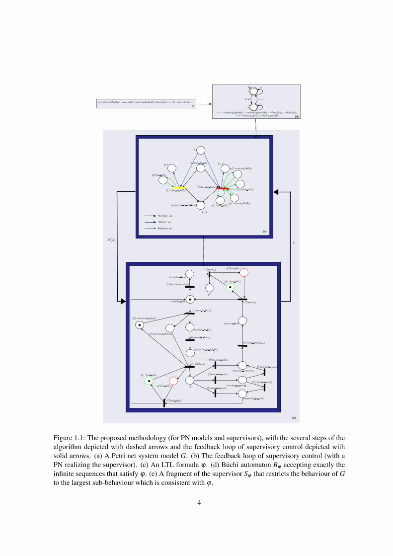
In Figure 1.1, we present a diagram illustrating the methodology for the construction of a PN

supervisor, given a PN model and an LTL specification. The dashed arrows represent the steps of

the method, and we will be explaining all the elements of the diagram throughout this thesis. To

summarize, we will start with a DES model of the system and a set of safety LTL formulas written

over the set of events of the system and a set of symbols describing the system’s states. For each of

these formulas, its translation to a Buchi automaton is built, following the method presented in [Gastin

and Oddoux, 2001]. The Buchi automaton is then appropriately composed with the model of the

system, according to the semantics previously defined. This composition provides a structure that

represents the smallest restriction – in the sense that any restriction which is more permissive in term

of events that can be fired by the system will not comply with the specification – of the behaviour

of the system that satisfies the LTL formula. Then, it is necessary to guarantee that this structure

is admissible and deadlock-free, so that it can be used as a realization of the supervisor that, when

run in closed-loop with the uncontrolled system, restricts its behaviour so that it satisfies the LTL

2

formula. We will describe the application of different known approaches to deal with this problem

to the structures resulting from our compositions, and also present an a priori restriction of the LTL

formulas, which can be used when the designer has a total knowledge of the system model, that

guarantees admissibility by construction.

While the procedure we present can be computationally expensive, all computations are performed

off-line.Thus, the execution of the supervisor resulting from our methodology requires very little in

terms of computational resources at run time, given that all the calculations, as complex as they might

be, are done before deploying the system. This is an important point because the supervisor will used

in a feedback-loop with the system, hence it is important that it is able to react to changes in the system

in a timely manner.

Although the work presented in this thesis is applicable to a wide array of systems – e.g., software

systems, manufacturing systems, air traffic control systems – we will focus on its application to robot

systems, mainly the coordination of multi-robot teams. Using LTL to specify and enforce coordina-

tion rules for teams of robots is quite natural. Furthermore, robotics is a field where innovation is

often associated with non-formal approaches. Novel ideas and concepts are typically introduced for

particular applications, through well-engineered systems, but lack guarantees concerning aspects such

as safety, predictability, performance, robustness and reliability, essential to support the acceptability

of robotic devices in factories, offices, hospitals or field (e.g., surveillance, medical care, planetary

exploration) scenarios. As previously discussed for DES in general, with the fast dissemination of

robot systems in the household and daily scenarios, where they must interact more frequently and in

a natural way with humans, these guarantees are essential.

We will focus most of our attention on the part of the methodology related with PNs. This is

justified by the fact that PNs are a more interesting and well-suited model for distributed systems,

allowing one to more easily scale to larger systems. Furthermore, the study of SC is much more

developed for FSA, so our contribution for SC of PNs is more substantial. In spite of that, we decided

also to present the methodology for FSA. The reason for this option is two-fold. Firstly, being a

more studied and simpler model, presenting the ideas for FSA first can help the reader to better grasp

the notions, thus facilitating the understanding of the PN version. Secondly, to have a fair way to

compare the FSA and PN approaches: we will be comparing the two approaches for one example,

giving evidence that for distributed systems PNs provide a better option for modelling, due to their

distributed state representation, instead of the exhaustive enumeration of the states required by FSA

models.

1.2 Related Work

Petri Net Modelling and Analysis

The PN formalism and its use for the modelling of DES has been widely studied in the literature. A

good and complete survey – however somewhat dated – can be found in [Murata, 1989]. There is also

3

(...)

(b)

(c)

(d)

(e)

Figure 1.1: The proposed methodology (for PN models and supervisors), with the several steps of thealgorithm depicted with dashed arrows and the feedback loop of supervisory control depicted withsolid arrows. (a) A Petri net system model G. (b) The feedback loop of supervisory control (with aPN realizing the supervisor). (c) An LTL formula ϕ . (d) Buchi automaton Bϕ accepting exactly theinfinite sequences that satisfy ϕ . (e) A fragment of the supervisor Sϕ that restricts the behaviour of Gto the largest sub-behaviour which is consistent with ϕ .

4

a considerable number of books and collections introducing and surveying the state-of-the-art of this

topic [Girault and Valk, 2002,David and Alla, 2010,Diaz, 2010,Reisig and Rozenberg, 1998a,Reisig

and Rozenberg, 1998b]. In these works, one can see PNs applied to a variety of domains, such as

manufacturing systems or telecommunication systems. A particular class of PNs, denominated work-

flow nets, is also being increasingly used to model business processes and develop process mining

techniques, e.g., [van der Aalst, 1998, van der Aalst and Stahl, 2011, Weidlich and van der Werf,

2012]. This wide array of application domains illustrates the flexibility enabled by PN models and

their extensions.

Regarding PN modelling in the robotics field, PNs are used for the modelling of (multi-)robot sys-

tems, due to their suitability to model distributed systems. There is a large amount of literature about

modelling methodologies both for robot systems [Costelha and Lima, 2007, Milutinovic and Lima,

2002,Wang et al., 1991,Ziparo and Iocchi, 2006] and multi-robot systems [Ziparo et al., 2008,Ziparo

et al., 2011, Costelha and Lima, 2012, Costelha and Lima, 2008, Sheng and Yang, 2005]. Our work

in not focused on modelling, so we keep the majority of the models presented in this thesis simple,

in order to facilitate the comprehension of the presented notions. In spite of that, in general, these

methodologies for robot system modelling can be followed while keeping our supervisor synthesis

method applicable.

In terms of qualitative analysis methodologies, the big bulk of the approaches can be classified in

one of the following classes:

1. Reachability approaches. These approaches entail building a finite representation of the state

space of the PN – the reachability graph when the PN is bounded or the coverability graph

when the PN is unbounded, i.e., when its state space is infinite. While with the reachability

graph, which completely represents the PN state space, one can solve all the problems that can

be solved for FSA, the same is not true for the coverability graph, which provides a finite rep-

resentation of an infinite state space, where some information is lost. These analysis techniques

are the simplest approach to solve PN analysis problems, because they reduce them to solving

a problem for FSA. Their main drawback is that they rely on explicitly building the state space

of the PN, hence they are affected by the state explosion problem. Reachability approaches

are described in all the introductory surveys on PNs [Girault and Valk, 2002, David and Alla,

2010, Diaz, 2010, Reisig and Rozenberg, 1998a, Reisig and Rozenberg, 1998b].

2. Structural approaches. These approaches have the least computational complexity, since they

rely only on analysing the PN structure, thus avoiding the state explosion problem. Their main

drawback is that only analysing the structure provides much less information, hence less prop-

erties can be decided. They are based on representing the PN in its matrix form and analysing

it to find substructures such as traps, siphons, place invariants or transition invariants. These

structures can be used to decide such properties as boundedness and liveness of the PN, inde-

pendently of the initial marking. One can also find descriptions of this type of approaches in

introductory surveys on PNs [Girault and Valk, 2002, David and Alla, 2010, Diaz, 2010, Reisig

5

and Rozenberg, 1998a, Reisig and Rozenberg, 1998b].

3. Linear algebraic approaches. This type of approach relies on the fact that the state evolution of

a PN can be seen as linear operations on integer matrices. The methods based on this approach

usually rely on translating the property to be analysed into an optimization problem, most of-

ten an integer linear program (ILP) [Schrijver, 1998]. It can be seen as a combination of the

previous approaches, where one uses the PN structure and firing rule to define an ILP. Solving

this ILP can be interpreted as a way to perform state exploration without explicitly building the

state space. In spite of that, this approach also has computational complexity issues, since it is

known that ILPs are NP-complete. A survey on these techniques is given on [Silva et al., 1998].

4. Petri net unfolding approaches. PN unfoldings were first introduced in [McMillan, 1992]. The

goal of using PN unfoldings it to avoid the state explosion problem while maintaining the abil-

ity to analyse the PN. To achieve this, a so called occurrence net is built from the original PN.

An occurrence net is a finite acyclic net that represents all the reachable markings of the PN.

This structure has been used in particular for model checking of PNs [Schroter and Khomenko,

2004, Esparza, 1994, Esparza and Heljanko, 2001]. Of particular interest is [Esparza and Hel-

janko, 2001], where the composition procedure used has many similarities with the one used

in this work. The differences are that there, the Buchi automaton “reads” the marking of the

PN and then evolves to a new state accordingly, while we evolve the Buchi automaton as the

PN changes state, disabling the firing of some events that would not satisfy the specification.

Furthermore, we allow for bounded places with an arbitrary number of tokens while the com-

position presented in [Esparza and Heljanko, 2001] only allows safe PNs. Unfoldings have also

been used for analysis of specific properties, such as existence of deadlocks [Melzer and Romer,

1997] or the coverability problem [Abdulla et al., 2004].

Supervisory Control

Supervisory control (SC) theory of DES was first introduced in the seminal paper [Ramadge and

Wonham, 1987]. A posterior overview paper by the same authors can be found in [Ramadge and

Wonham, 1989]. This is known as the Ramadge-Wonham framework and most of the works on the

control of DES ever since have been based on it. It provides an analogy to DES of the classical

control theory for continuous systems. More recent books dealing with SC theory are [Cassandras

and Lafortune, 2006, Kumar and Garg, 1995, Seatzu et al., 2012]. The reference [Seatzu et al., 2012]

is a very recent collection that deals with SC of both FSA and PN and provides a thorough look on

the state-of-the-art of this topic.

Regarding temporal logic based SC of FSA models, [Jiang and Kumar, 2006b, Jiang and Kumar,

2006a] describe a methodology for building a state-based supervisor from temporal logic specifica-

tions. In this approach both the system and the goal specifications are encoded as a temporal logic

formula, which is in turn translated into an FSA that satisfies it. The work in [Gromyko et al., 2006]

6

presents a tool to perform controller synthesis using the NuSMV [Cimatti et al., 2002] model checking

tool. Contrary to our method, the temporal logic formulas are written only over the state space of the

system, thus direct reasoning about sequences of events is not allowed. In [Lacerda and Lima, 2008]

a similar method, that allows writing specifications only about events is described. While the applica-

bility of these works is limited to FSA models, ours offers the possibility of building PN supervisors,

which are, in general, more compact, thus offering the possibility to scale to larger systems.

The control of PNs has also been the subject of study. A comprehensive survey on available

methods for control of PNs, including controlled PNs, a discussion on SC with language specifications

and supervision based on place invariants is provided in [Holloway et al., 1997].

The use of controlled PNs, was first introduced in [Krogh, 1987, Ichikawa and Hiraishi, 1988].

Controlled PNs extend classical PNs by introducing external enabling conditions, denominated con-

trol places. A (state-based) control policy for this kind of PNs is a function that maps each marking

to a token distribution in the control places. Thus, the tokens in these places do not change due to the

firing rule of the PN, as with the tokens in standard places. Their token distribution for each marking

is given by the control policy. In our work, we aim to have the supervisor realized as a PN so that the

closed-loop behaviour of the system can be analysed using standard PN techniques. For this reason

we will not get into more details on controlled PNs.

The amount of work on SC of PNs based on the Ramadge-Wonham framework, i.e., with lan-

guage specifications, is not very extensive. This is probably due to some undesirable properties of

PN languages. For example, in general PN languages are not closed under the supremal controllable

sublanguage operator [Giua and DiCesare, 1994a], which makes it impossible to define general meth-

ods to find least restrictive admissible supervisors realized as PNs. In spite of that, in some cases it

is possible to design PN supervisors based on the Ramadge-Wonham framework and some work has

been done on defining a SC theory of PNs based on that framework [Giua and DiCesare, 1994b,Giua

and DiCesare, 1991, Giua and DiCesare, 1995]. For a thorough state-of-the-art compilation of these

results, we refer the reader to [Giua, 2013]. Furthermore, it is shown there that it is possible to check

if the supervisor is admissible and non-blocking. These results will be used in our work, hence we

will describe them in greater detail in Chapter 5.

In [Kumar and Holloway, 1996], it is shown that the problem of synthesizing the minimally re-

strictive supervisor so that the controlled system generates the supremal controllable sublanguage is

reducible to a forbidden marking problem on the PN resulting from the composition of the system

with the specification. Furthermore, a state-based control policy for minimally restrictive supervision

is defined. This control policy has the drawback of requiring the online calculation of coverability of

a set of markings at each step, which is an exponential calculation in the number of places of the PN

resulting from the composition, thus greatly reducing its applicability on a feedback loop.

A widely used approach for supervisory control of PNs is the so called supervision based on place

invariants (SBPI) or generalized mutual exclusion constraints (GMEC) [Giua et al., 1992, Iordache

and Antsaklis, 2006b, Wu et al., 2002, Iordache and Antsaklis, 2002, Moody and Antsaklis, 1998,

7

Iordache and Antsaklis, 2006a]. In this approach, the specifications are written as linear constraints

on the reachable markings of the system and the number of firings of each transition. This line of

work has a good theoretical foundation and deals with several important notions of the theory of SC,

such as controllability [Basile et al., 2006], observability [Moody and Antsaklis, 1999], deadlock

avoidance [Iordache et al., 2002]. This approach has some properties that we also want to include in

our methodology:

• The supervisor is realized as a PN, enabling the use of PN analysis methods to study the closed-

loop system. Note that, as stated before, it is proven in [Giua and DiCesare, 1994a] that having

PN realizations of supervisors negates the possibility of obtaining least restrictive supervisors.

In spite of that, we argue that being able to use all the PN analysis tools to study the closed-loop

behaviour of the system and having a PN implementation of the control-law, which does not

require extensive calculations to be executed online, makes up for this drawback.

• It is a structural approach, i.e., the construction of the supervisor is done by only takes places

and transitions of the PN model of the plant, avoiding the state space explosion problem.

A major difference between GMEC and the work presented here is related with the way the rules to be

fulfilled are specified. We argue that the use of LTL as the specification language is more suitable than

writing linear constrains, especially for specification of coordination rules for multi-robot systems. We

will further discuss the relation between our approach and GMEC in Chapter 5.

There is also work on enforcing liveness in PNs, i.e., using SC to force all the transitions of

the PN to remain eventually fireable. The work of [Sreenivas, 1997, Sreenivas, 2012] deals with the

foundations of this problem while [Iordache and Antsaklis, 2003] uses the SBPI framework to solve

it in a non least restrictive manner.

In the robotics domain DES modelling and supervision have been used for a number of applica-

tions. In [Lee et al., 2005], a technique to design deadlock-free PN supervisors that avoid collisions

between robots is presented. This method is based on defining regions that are considered shared re-

sources, and then appropriately building PNs that disallow the usage of these resources by more than

one robot. The method is restricted to this application, while ours allows the specification of more

general behaviours. In [Kosecka and Bogoni, 1994], the authors present a DES-based framework for

modelling behaviours and tasks for heterogeneous robotic agents, presenting examples for common

robot tasks such as navigation and obstacle avoidance. The work of [Ricker et al., 1996] deals with

performance of dexterous manipulation. A more recent work [Chen et al., 2012a] uses GRAFCET, a

PN based graphical programming language for hardware implementation.

Temporal Logic Based Control of Robot Tasks

In the last years, there has been a great deal of work based on formal approaches to robotics. Most of

this work is inspired on symbolic control, with [Belta et al., 2007] providing a survey of the state-of-

the-art at the time and also posing the challenges to be tackled in the field, providing inspiration for

8

most of the succeeding work. The main goal of this type of approach is to automatically build robot

controllers from high level specifications, most commonly given in LTL.

Regarding motion planning methods, where the goals are defined as LTL formulas, there has been

work both on robot [Kloetzer and Belta, 2008b,Fainekos et al., 2005] and multi-robot systems [Kloet-

zer and Belta, 2006, Kloetzer and Belta, 2007, Kloetzer and Belta, 2008a, Loizou and Kyriakopoulos,

2004]. These works have been extended to handle the uncertainty inherent to the mobile robotics do-

main, by using stochastic models such as Markov decision processes [Ulusoy et al., 2012c,Cizelj and

Belta, 2013, Chen et al., 2012b, Lahijanian et al., 2009] and also to obtain robust optimal paths when

there is uncertainty on the robot travelling times, both in single-robot [Smith et al., 2011, Wolff et al.,

2012] and multi-robot [Ulusoy et al., 2012a, Ulusoy et al., 2012b] scenarios. Using LTL to define

the goals allows the specification of not only a goal region but also more intricate movements such

as visiting a set of regions sequentially or travel between regions infinitely often. In these works, the

LTL formulas only state when certain regions of a workspace should be visited or avoided. Further-

more, these approaches do not allow sensor readings, building controllers that are not able to react to

changes in the environment.

The work in [Kress-Gazit et al., 2009, Kress-Gazit et al., 2008, Kress-Gazit et al., 2007b] also

deals with motion planning with temporal logic goals but allowing the robot to also react to sensor

readings and perform actions other than navigation. This work has been extended to handle partially

unknown environments [Sarid et al., 2012], uncertainty in sensor readings [Johnson et al., 2012]

and to define a framework as user-friendly as possible, by providing the designer with the ability to

define the specifications in structured english [Kress-Gazit et al., 2007a] and giving feedback when the

specification cannot be satisfied [Raman and Kress-Gazit, 2012a, Raman and Kress-Gazit, 2012b]. In

these approaches, both the system and the goal specifications are encoded as a temporal logic formula,

while we encode the system as an FSA or a PN. For the case of PN modelling specifically, this allows

for the modelling of larger and more distributed systems.

There has also been some more work linking temporal logics and FSA in a planning framework.

In this work, planning algorithms over a domain given as an FSA, where the states correspond to

sets of propositional symbols and the goal is given as a temporal logic formula over those symbols,

are defined [Pistore and Traverso, 2001, De Giacomo and Vardi, 2000, Cimatti et al., 2003]. This, of

course, requires a state exploration to obtain the plan, which is something we will not be dealing with

in our work. Our goal is to keep the system “inside” a given type of behaviour, hence we can avoid

the complexity issues that arise with state space exploration.

Finally, LTL has also been used in a more classical control-theoretic approach, for hybrid con-

trol. In [Tabuada and Pappas, 2006, Tabuada and Pappas, 2003], the design of controllers enforcing

LTL formulas for linear systems, based on the existence of finite bisimulations for linear systems, is

described. Other works dealing with this topic are [Aydin Gol et al., 2012, Fainekos et al., 2006].

9

1.3 Thesis Goals and Contributions

The goal of our methodology to design supervisors is to provide the designer with a formal framework

under which:

1. The unsupervised system is modelled by the designer using a DES representation (FSA or PN),

and represents all possible system evolutions in its environment;

2. An FSA or PN supervisor realization is automatically constructed for each specification, written

by the designer as an LTL formula that expresses a desired behaviour for a given task to be

carried out.

The main contributions of this work can be summarized in the following points:

• A semantics to evaluate LTL formulas over PNs, where one can reason both about linear com-

binations of the number of tokens in each place plus the labels of transitions, is presented.

• A composition between the Buchi automaton obtained from an LTL formula and a PN model,

that yields a PN that restricts the behaviour of the original PN to the one that satisfies the LTL

formula is defined.

• A discussion on approaches to obtain admissible and deadlock-free supervisors is provided. The

standard notion of uncontrollable marking usually used in the literature is shown to be incorrect.

A new, sound version is proposed and some results for checking admissibility for deterministic

PN supervisors are proved for the new definition.

• An application of PN-based SC to a real world multi-robot scenario is described.

1.4 Document Organization

We start the remainder of the work by introducing the modelling formalisms, in Chapter 2. We will

define three different system models: FSA where the states have a symbolic propositional description,

PNs where the states have a symbolic propositional description, and PNs where the states have a linear

algebraic propositional description.

In Chapter 3, we focus on describing the formalism used to write the specifications that the system

models must fulfil. We introduce LTL, define its semantics for each of the system models and discuss

safe LTL formulas, the fragment of LTL that will be used in the methodology.

Chapters 4 and 5 contain the main theoretical contributions of the thesis. In Chapter 4 we pro-

vide algorithms for composing the system models with the Buchi automata obtained from the LTL

formulas, creating a coarse structure for the supervisor. In Chapter 5 we focus on ways of refining

that structure so that the supervisor realizations are admissible and deadlock-free. For the case of PNs

we also show that the notion of uncontrollable marking usually used in the procedures to check for

10

supervisor admissibility is not soundly defined, by means of a counter example. Then we redefine it

in a proper way, and present algorithms to check for admissibility and deadlock-freeness based on this

new notion of uncontrollable marking. We also point out the limitations of PNs in the scope of SC

theory and discuss ways of circumventing these limitations.

In Chapter 6, we show the more practical contributions of the work, which are focused on the

application of the methodology to single and multi-robot systems:

• First, a simulated soccer scenario, where a team of robots must coordinate passes and move-

ments towards the ball. In this example, we show how to build (centralized) FSA supervisors

and both centralized and decentralized PN supervisors, comparing the sizes of the obtained

structures and the scalability of the different approaches.

• Second, an implementation on a real social robot where interaction rules with a human are given

to the robot in the form of LTL formulas.

• Finally, a larger-scale scenario, where a team of real robots must coordinate in order to perform

surveillance tasks, in a mock-up scenario, is tackled.

Finally, in Chapter 7, a discussion about the methodology is provided, along with a discussion of

what was accomplished and an extensive list of possible future work routes.

11

CHAPTER 2

System Modelling

In this chapter, we introduce the modelling formalisms. We start by showing how to model a system

using FSA equipped with a state description function. Then we show two approaches for PN mod-

elling of the system. First, a version that mirrors the FSA model, where we use a subset of the places

of the PN to represent the truth value of atomic propositions, followed by a more general version

where the atomic propositions are considered to be linear inequalities over markings. In the follow-

ing, let Σ be a finite alphabet, Σ∗ the set of all finite strings built from Σ (including the empty string ε)

and Σω the set of all infinite strings that can be build from Σ. Also, given a finite set A, let |A| ∈ N be

the number of elements of A.

2.1 Finite State Automata

In this section, we describe finite state automata (FSA), one of the tools we will use to model the

systems. We also equip the FSA with a set of state description symbols and a function that maps

each state of the FSA to the state description symbols that are true in that state. This state description

symbols will, in conjunction with the set of events, be used to describe the behaviours of the system.

Definition 2.1.1 (Finite State Automaton). A finite state automaton (FSA) is a tuple A = 〈Q,Σ,δ ,Q0〉where:

• Q is a finite set of states;

• Σ is a finite alphabet;

• δ : Q×Σ→ Q (deterministic case) or δ : Q×Σ→ 2Q (non-deterministic case)1 is the possibly1We introduce the notion of non-deterministic automaton because it will be needed when we introduce Buchi automata.

In our definition, we do not take into account the possibility of the empty string ε labelling transitions.

13

partial transition function;

• Q0 = q0 ∈Q is the initial state (deterministic case) or Q0 ⊆Q is the set of possible initial states

(non-deterministic case).

To simplify the notation, we define the active symbol function, a function that maps each state of

an FSA to the symbols that are active in that state.

Definition 2.1.2 (Active Symbol Function). Let A = 〈Q,Σ,δ ,Q0〉 be an FSA. The active symbol

function ΓA : Q→ 2Σ is defined as:

ΓA(q) = {a ∈ Σ | δ (q,a) is defined} (2.1)

Definition 2.1.3 (ω-Language Generated by a deterministic FSA). Let A = 〈Q,E,δ ,q0〉 be an FSA.

The language generated by A is defined as:

L (A) = {σ = (e1,q1)(e2,q2)... ∈ (E×Q)ω | qi+1 = δ (qi,ei+1) for all i ∈ N} (2.2)

The members of L (A) are the infinite sequences of events and states that can occur while starting

in q0 and following the transition function δ , i.e., for t ∈ N, σt = (e,q) means that the system is in

state q at time2 t, and we reached q by firing event e. Note that q1 must be reachable from the initial

state q0 through the firing of e1. We will deal with the fact that q0 does not appear in the language by

adding a dummy state, as will be explained later.

We will use deterministic FSA to model DES. In DES models, the alphabet is a set of events3 E

and, in order to have a propositional description of the states, we equip the FSA with a set of state

description symbols.

Definition 2.1.4 (FSA System Model). An FSA system model is a tuple G= 〈Q,E,δ ,q0,D,µ〉where:

• 〈Q,E,δ ,q0〉 is a deterministic FSA. We consider L (G) equal to the language generated by

〈Q,E,δ ,q0〉, according to Definition 2.1.3;

• D is a finite set of state description symbols;

• µ : Q→ 2D is a function that maps each state into the set of state description symbols that are

true in that state.

We will be interested in the ω-language generated by FSA system models, which represents the

set of all possible infinite behaviours of the system. The language will contain both the sequence of

events and states visited.2In this work, we consider time as discrete steps and that the system is in the initial state at time 0.3We defined both deterministic and non-deterministic FSA because we will use deterministic FSA to model the system,

but we will need the notion of non-deterministic automata later, when we discuss Buchi automata. In this section, we assumethat all the FSA are deterministic. We also left the alphabet set arbitrary because for Buchi automata the alphabet is not aset of events. We will refer to the active symbol function as active event function when dealing with FSA models of DES.

14

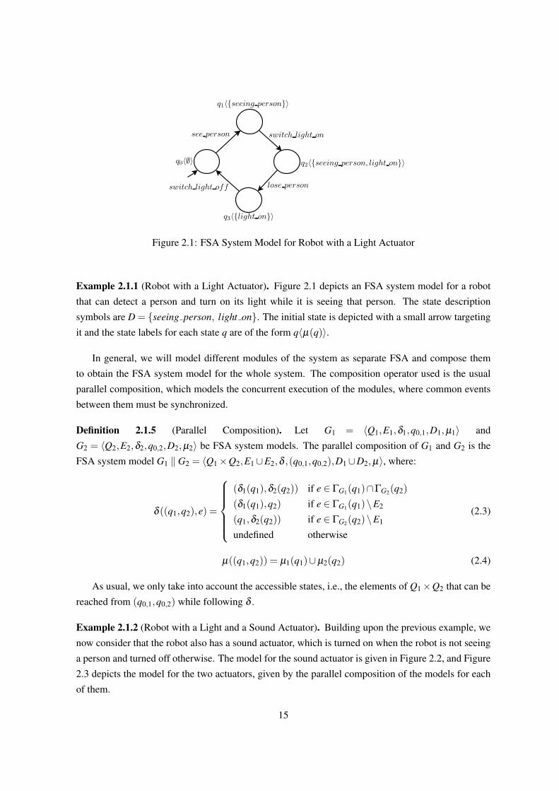
Figure 2.1: FSA System Model for Robot with a Light Actuator

Example 2.1.1 (Robot with a Light Actuator). Figure 2.1 depicts an FSA system model for a robot

that can detect a person and turn on its light while it is seeing that person. The state description

symbols are D = {seeing person, light on}. The initial state is depicted with a small arrow targeting

it and the state labels for each state q are of the form q〈µ(q)〉.

In general, we will model different modules of the system as separate FSA and compose them

to obtain the FSA system model for the whole system. The composition operator used is the usual

parallel composition, which models the concurrent execution of the modules, where common events

between them must be synchronized.

Definition 2.1.5 (Parallel Composition). Let G1 = 〈Q1,E1,δ1,q0,1,D1,µ1〉 and

G2 = 〈Q2,E2,δ2,q0,2,D2,µ2〉 be FSA system models. The parallel composition of G1 and G2 is the

FSA system model G1 ‖ G2 = 〈Q1×Q2,E1∪E2,δ ,(q0,1,q0,2),D1∪D2,µ〉, where:

δ ((q1,q2),e) =

(δ1(q1),δ2(q2)) if e ∈ ΓG1(q1)∩ΓG2(q2)

(δ1(q1),q2) if e ∈ ΓG1(q1)\E2

(q1,δ2(q2)) if e ∈ ΓG2(q2)\E1

undefined otherwise

(2.3)

µ((q1,q2)) = µ1(q1)∪µ2(q2) (2.4)

As usual, we only take into account the accessible states, i.e., the elements of Q1×Q2 that can be

reached from (q0,1,q0,2) while following δ .

Example 2.1.2 (Robot with a Light and a Sound Actuator). Building upon the previous example, we

now consider that the robot also has a sound actuator, which is turned on when the robot is not seeing

a person and turned off otherwise. The model for the sound actuator is given in Figure 2.2, and Figure

2.3 depicts the model for the two actuators, given by the parallel composition of the models for each

of them.

15

Figure 2.2: FSA System Model for a Robot with a Sound Actuator

Figure 2.3: FSA System Model for a Robot with a Light and Sound Actuator

16

2.2 Petri Nets

The use of FSA allows us to model a good amount of systems, but, especially when dealing with

distributed systems, the need to enumerate all possible states of the system in the model becomes both

cumbersome and computationally inefficient. Changing the modelling formalism to Petri nets (PN)

allows us to model richer systems, since PNs are known to be more expressive than FSA, in terms

of generated languages, and also provides a more compact way of describing our systems because,

using PNs, there is no need of enumerating all the states the system can be in. We argue that, being

more compact, the use of PNs to model the uncontrolled system allows the control of more complex

systems than both modelling the system as an FSA or the encoding of a system as a temporal logic

formula, being the best suited formalism (of the ones referred here) to model distributed systems.

We start by providing a brief overview on PN structures, starting by the definition of the different

elements of a PN.

Definition 2.2.1 (Petri Net Structure). A Petri net structure is a tuple N = 〈P,T,W−,W+,M0〉 where:

• P is a finite, not empty, set of places;

• T is a finite, not empty, set of transitions;

• W− ∈ N|P|×|T | is the input matrix;

• W+ ∈ N|P|×|T | is the output matrix;

• M0 ∈ N|P| is the initial marking.

The input matrix represents arc weights between places and transitions while the output matrix

represents arc weights between transitions and places. This means that a PN structure is a weighted

bipartite graph, where each node is either a place or a transition. The initial marking M0 is a vector of

size |P| that represents the initial state of the system, with M0(p) = q meaning that there are q tokens

in place p in the initial state.

We will use the places and transitions themselves as the indices of the matrices and vectors, e.g.,

given p ∈ P and t ∈ T , we use W−(p, t) to represent the entry W−i j that corresponds to the arc weight

from p to t. We will also use the incidence matrix W =W+−W−. Note that, in general an incidence

matrix W does not uniquely define a pair W− and W+ of input and output matrices. However, when the

PN is self-loop free – i.e., if W+(p, t)> 0, then W−(p, t) = 0 and if W−(p, t)> 0, then W+(p, t) = 0

– the incidence matrix is enough to uniquely define W− and W+:

W−(p, t) =

{−W (p, t) if W (p, t)< 0

0 otherwise(2.5)

W+(p, t) =

{W (p, t) if W (p, t)> 0

0 otherwise(2.6)

17

We will also use the notions of pre and post set of a node in a PN.

Definition 2.2.2 (Presets and Postsets). Let N = 〈P,T,W−,W+,M0〉 be a PN structure, p ∈ P and

t ∈ T . We define the following vectors:

• The preset of p, •p ∈ N|T |, such that •p(t) = W+(p, t). If •p(t) > 0, we say that t is in the

preset of p.

• The postset of p, p• ∈ N|T |, such that p•(t) = W−(p, t). If p•(t) > 0, we say that t is in the

postset of p.

• The preset of t, •t ∈N|P|, such that •t(p) =W−(p, t). If •t(p)> 0, we say that p is in the preset

of t.

• The postset of t, t• ∈ N|P|, such that t•(p) = W+(p, t). If t•(p) > 0, we say that p is in the

postset of t.

The dynamics of a PN are defined by the firing rule, which determines the flow of tokens between

places, thus specifying how the initial marking can evolve.

Definition 2.2.3 (Firing Rule). Let N = 〈P,T,W−,W+,M0〉, t ∈ T and M ∈ N|P|. Transition t is said

to be active if for all p ∈ P, •t(p)≤M(p). A transition t active in a marking M can fire, resulting in

the marking M′ = M−W−(., t)+W+(., t) = M− •t + t•. This is denoted M t→M′.

Using the firing rule, one can define firing sequences and the set of reachable markings of a given

PN structure.

Definition 2.2.4 (Firing Sequence). Let N = 〈P,T,W−,W+,M0〉 be a PN structure. A finite firing

sequence from a given marking M is a sequence of transitions τ = t1t2...tn ∈ T ∗ such that there exists

markings M1, ...,Mn such that:

M t1→M1t2→M2

t2→ ...tn→Mn (2.7)

An infinite firing sequence from a given marking M is a sequence of transitions τ = t1t2... ∈ T ω such

that there exists markings M1,M2, ... such that:

M t1→M1t2→M2

t2→ ... (2.8)

Finite firing sequences will be used to define reachable markings in the PN, while infinite firing

sequences will be used to define the language generated by the PN.

Definition 2.2.5 (Markings Notation). Let N = 〈P,T,W−,W+,M0〉, M ∈ N|P| and τ ∈ T ∗. We write:

• M τ→M′ to denote that the firing sequence τ drives N from marking M to marking M′;

• (M τ→) to denote that N can fire the sequence τ from M;

18

• (If (M0τ→)) Mτ to denote the marking reached after firing τ from M0.

Definition 2.2.6 (Reachable Markings). The set of all reachable markings by N = 〈P,T,W,M0〉 is

denoted as:

R(N) = {Mτ | τ ∈ T ∗ and (M0τ→)} (2.9)

Note that all reachable markings are of the form Mτ =M0+Wwτ , where wτ is the vector of natural

numbers of size |T | for which the i-th entry is the number of occurrences in τ of the i-th transition.

This vector is denominated firing count vector. However, the converse is not true: in general, there

exists w ∈ N|T | such that M0 +Ww is not a reachable marking. This is due to the fact that a transition

t is only active when •t ≤M.

We will be interested in the languages generated by PNs, hence we add labels to the transitions.

Furthermore, since we will only use PNs to model DES, we can already assume that the alphabet set

is a set E of events.

Definition 2.2.7 (Labelled Petri Net). A labelled Petri net is a tuple L = 〈P,T,W−,W+,M0,E, `〉where:

• 〈P,T,W−,W+,M0〉 is a PN structure. We consider R(L) equal to the set of reachable markings

of 〈P,T,W−,W+,M0〉, according to Definition 2.2.6;

• E is the finite set of events;

• ` : T → E is the labelling function, that assigns to each transition an event from E.

We extend the labelling function to a function ` : T ∗→ E∗ and ` : T ω → Eω as usual:

• `(t1...tn) = `(t1)...`(tn);

• `(t1t2...) = `(t1)`(t2)....

We require the PNs in this work to be deterministic, in the sense that a sequence of labels uniquely

defines the sequence of visited markings. This is done because we will use the PN model to build the

PN realization of the supervisor. As will be seen later, a supervisor is formally a function, and, in order

to represent a function, a PN must be deterministic, because otherwise the result for a given input will

not be unequivocally defined. Furthermore, the algorithms for admissibility and deadlock-freeness

checking presented on Chapter 5 requires deterministic PNs.

Definition 2.2.8 (Deterministic Petri net). A labelled PN L is deterministic if for all t, t ′ ∈ T and

M ∈ R(L):

If

M t→M′

M t ′→M′′

M′ 6= M′′then `(t) 6= `(t ′) (2.10)

19

Definition 2.2.9 (Reached Marking). Let L = 〈P,T,W−,W+,M0,E, `〉 be a deterministic labelled PN

and s = s0...sk ∈ E∗. If there exists a transition sequence τ = t0...tn such that `(ti) = si for all i ∈{0, ...,n} and (M0

τ→), then we define the marking reached after the firing of s as Ms = Mτ .

Note that Ms is well-defined, in the sense that given, s ∈ E∗, Ms is unique. This is a direct con-

sequence of assuming that the PNs are deterministic. Henceforth, we will assume that all PNs are

deterministic.

Definition 2.2.10 (Active Event Function). Let L = 〈P,T,W−,W+,M0,E, `〉 be a labelled PN. We

define the function ΓL : R(L)→ 2E as:

ΓL(M) = {e ∈ E | exists t ∈ T such that `(t) = e and t is active in M} (2.11)

As with FSA system models, we will be interested in the ω-language generated by labelled PNs,

which represents the set of all possible infinite behaviours of the system. The language will also

contain both the sequence of events and states visited, taking into account that in this case the states

visited by the system are represented by markings.

Definition 2.2.11 (Language Generated by a Labelled Petri Net). Let L = 〈P,T,W−,W+,M0,E, `〉 be

a labelled PN. The language generated by L is defined as:

L (L) ={(`(t1),M1)(`(t2),M2)... ∈ (E×R(L))ω | such that M0

t1→M1t2→M2

t3→ ...}

(2.12)

The members of L (L) are the infinite sequences of event and marking pairs that can occur while

starting in M0 and following the PN firing rule, i.e., for t ∈ N, σt = (e,M) means that the system is in

marking M at time t, and we reached M by firing a transition labelled by event e. As with the language

generated by FSA system models, note that M1 must be reachable from the initial marking M0 through

the firing of t1. We will deal with the fact that M0 does not appear in the language by adding a dummy

place and a dummy transition, and changing the initial marking, as will be explained later.

Before we present the PN system models, we will introduce the notion of complement place of a

bounded place. This notion is central for the definition of both system models, and is defined for the

PN structure (i.e., it is independent of transition labels).

Definition 2.2.12 (Place Bound). Let N = 〈P,T,W−,W+,M0〉 be a PN structure and p ∈ P. A bound

for p is a number k ∈ N such that M(p) ≤ k for all M ∈ R(N). If there exists a bound for p we say

that p is bounded, otherwise we say that p is unbounded. If there exists M ∈ R(N) such that M(p) = k

we say that k is the strict bound.

Calculating if a bound exists and its value for a given place can be done using PN analysis tech-

niques.

20

Definition 2.2.13 (Complement Place). Let N = 〈P,T,W−,W+,M0〉 be a PN structure, p ∈ P. A

complement place for p is a place pc ∈ P such that, for all t ∈ T :

W+(pc, t)−W−(pc, t) =W−(p, t)−W+(p, t) (2.13)

We now prove some properties of the complement place. These properties are known, and can be

easily proved. We chose to include the proofs here to help the reader have a better grasp of this notion.

Proposition 2.2.1 (Complement Place Properties). Let N = 〈P,T,W−,W+,M0〉 be a PN structure,

p ∈ P, and pc ∈ P a complement place for p. Then:

1. p is a complement place for pc;

2. For all M ∈ R(N), M(p)+M(pc) = k is constant;

3. k is a bound for p and pc.

Proof.

1. By definition of complement place, this property clearly holds;

2. Let M ∈ R(N). Then M is of the form M = M0 +Wwτ , where wτ is the firing count vector for a

sequence τ ∈ T ∗ such that M0τ→M. Then:

M(p)+M(pc) = M0(p)+W (p, .)wτ +M0(pc)+W (pc, .)wτ

= M0(p)+ ∑t∈T

W (p, t)wτ(t)+M0(pc)+ ∑t∈T

W (pc, t)wτ(t)

= M0(p)+M0(pc)+ ∑t∈T

(W (p, t)+W (pc, t))wτ(t)

= M0(p)+M0(pc)+ ∑t∈T

(W+(p, t)−W−(p, t)+W+(pc, t)−W−(pc, t))wτ(t)

= M0(p)+M0(pc)+ ∑t∈T

(W+(p, t)−W−(p, t)+W−(p, t)−W+(p, t))wτ(t)

= M0(p)+M0(pc)

3. This is a direct consequence of the previous point.

Example 2.2.1 (Complement Place). In Figure 2.4, we depict a PN where place p2 is a complement

place of p1 (and, according to 2.2.1, vice-versa):

• W+(p2, t1)−W−(p2, t1) =−1 =W−(p1, t1)−W+(p2, t1);

• W+(p2, t2)−W−(p2, t2) = 2 =W−(p1, t2)−W+(p2, t2);

21

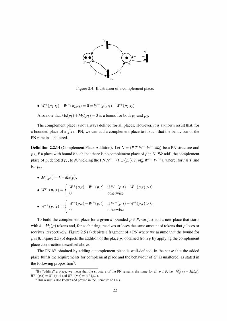
Figure 2.4: Illustration of a complement place.

• W+(p2, t3)−W−(p2, t3) = 0 =W−(p1, t3)−W+(p2, t3).

Also note that M0(p1)+M0(p2) = 3 is a bound for both p1 and p2.

The complement place is not always defined for all places. However, it is a known result that, for

a bounded place of a given PN, we can add a complement place to it such that the behaviour of the

PN remains unaltered.

Definition 2.2.14 (Complement Place Addition). Let N = 〈P,T,W−,W+,M0〉 be a PN structure and

p∈ P a place with bound k such that there is no complement place of p in N. We add4 the complement

place of p, denoted pc, to N, yielding the PN Nc = 〈P∪{pc},T,Mc0,W

c−,W c+〉, where, for t ∈ T and

for pc:

• Mc0(pc) = k−M0(p);

• W c−(pc, t) =

{W+(p, t)−W−(p, t) if W+(p, t)−W−(p, t)> 0

0 otherwise

• W c+(pc, t) =

{W−(p, t)−W+(p, t) if W−(p, t)−W+(p, t)> 0

0 otherwise

To build the complement place for a given k-bounded p ∈ P, we just add a new place that starts

with k−M0(p) tokens and, for each firing, receives or loses the same amount of tokens that p loses or

receives, respectively. Figure 2.5 (a) depicts a fragment of a PN where we assume that the bound for

p is 8. Figure 2.5 (b) depicts the addition of the place pc obtained from p by applying the complement

place construction described above.

The PN Nc obtained by adding a complement place is well-defined, in the sense that the added

place fulfils the requirements for complement place and the behaviour of Gc is unaltered, as stated in

the following proposition5.

4By “adding” a place, we mean that the structure of the PN remains the same for all p ∈ P, i.e., Mc0(p) = M0(p),

W c−(p, t) =W−(p, t) and W c+(p, t) =W+(p, t).5This result is also known and proved in the literature on PNs.

22

Figure 2.5: Illustration of the complement place construction.

Proposition 2.2.2. Let N be a PN structure, p ∈ P a place with bound k such that there is no com-

plement place for p in N, Nc the PN obtained by adding the complement place pc for p and τ ∈ T ∗.

Then, M0τ→M if and only if Mc

0τ→Mc, where:

Mc(p′) =

{M(p′) if p′ ∈ P

k−M(p) if p′ = pc(2.14)

Proof. Note that it is clear that if Mc0

τ→Mc, then M0τ→M. This is true because, by adding a place,

we can only restrict the behaviour of the original PN. Furthermore, the initial markings in N and Nc

coincide for p 6= pc, as do the pre and postsets. Thus, we just need to show that, given τ ∈ T ∗, if

M0τ→M, then Mc

0τ→Mc. We will show that Mc

0τ→Mc by induction on the length of τ .

1. |τ|= 0, i.e., τ = ε:

In this case we need to analyse the initial marking Mc0, which satisfies the requirement by defi-

nition.

2. |τ|= n+1, i.e., τ = τ ′t, τ ′ ∈ T ∗, t ∈ T : By hypothesis, we have that:

Mcτ ′(p′) =

{Mτ ′(p′) if p′ ∈ P

k−Mτ ′(p) if p′ = pc(2.15)

Hence, we need to prove that:

(i) Given that t is active in Mτ ′ for N, then it is also active for Mcτ ′ for Nc, i.e., given that

(Mτ ′t→), then (Mc

τ ′t→):

23

We assume thatgiven a it is true that (Mτ ′t→), but not (Mc

τ ′t→). Hence, we have W c−(p, t)=

W−(p, t)≤Mτ ′(p) for all p ∈ P. Thus, t not being active in Mcτ ′ must be due to place pc,

i.e., W c−(pc, t)>Mcτ ′(pc) = k−Mτ ′(p). According to the definition, we have two possible

cases for the value of W c−(pc, t). First if W c−(pc, t) = 0, then Mτ ′(p)> k, which contra-

dicts the fact that k represents the maximum amount of tokens that can be in places p ∈ P.

Second, if W c−(pc, t) =W+(p, t)−W−(p, t), then Mτ ′(p)+W+(p, t)−W−(p, t)> k, i.e.,

Mτ ′t(p) > k,which also contradicts the fact that k represents the maximum amount of to-

kens that can be in places p ∈ P.

(ii) The marking obtained by firing t in Mcτ ′ satisfies the equality stated in the proposition, i.e.:

Mcτ ′t(p′) =

{Mτ ′(p′)−W−(p′, t)+W+(p′, t) if p′ ∈ P

k− (Mτ ′(p)−W−(p, t)+W+(p, t)) if p = pc(2.16)

For p′ ∈ P, the equality is obvious because W c− coincides with W− and W c+ coincides

with W+. For p′ = pc, we have:

Mcτ ′t(pc) = Mc

τ ′(pc)−W c−(pc, t)+W c+(pc, t)

= k−Mτ ′(p)−W c−(pc, t)+W c+(t, pc)

From the definition of W c− and W c+, we need to analyse two possible cases. First,

W c−(pc, t) = 0 and W c+(pc, t)≥ 0. In this case:

Mcτ ′t(pc) = k−Mτ ′(p)+W c+(pc, t)

= k−Mτ ′(p)+W−(p, t)−W+(p, t)

= k− (Mτ ′(p)−W−(p, t)+W+(p, t))

Second W c−(pc, t)≥ 0 and W c+(pc, t) = 0. In this case:

Mcτ ′t(pc) = k−Mτ ′(p)−W c−(pc, t)

= k−Mτ ′(p)− (W+(p, t)−W−(p, t))

= k− (Mτ ′(p)−W−(p, t)+W+(p, t))

Hence the proof is completed.

A direct consequence of this proposition is that we can add complement places to labelled PNs

without changing the generated language.

Corollary 2.2.1. Let L = 〈P,T,W−,W+,M0,E, `〉 be a PN system model and

Lc = 〈Pc,T,W c−,W c+,Mc0,E, `〉 be the labelled PN obtained from adding a complement place to

24

the PN structure 〈P,T,W−,W+,M0〉. Then L (L) = L (Lc).6

From the proposition above, we can assume that all places for which we know a bound k have

a complement place defined in the PN. In the cases where it is not, we add the complement place

for p using the construction we just described. Hence, from now on we will omit from the figures

the complement places that are not required to specify a given behaviour, which are added using the

complement place construction.

Using the notion of complement place, we will use two different approaches for modelling DES

as PNs:

• A symbolic approach, similar to the FSA approach. In this approach, the markings are described

by a set of state description symbols. This is achieved by defining a subset of places that

correspond to the truth value of state description symbols.

• A linear algebraic approach, which takes advantage of the fact that markings have a linear al-

gebraic description7 We will use this fact to define the atomic propositions for our specifications

as linear constraints over the markings.

It is important to note that the symbolic approach is subsumed by the algebraic approach, as we

will show later. In spite of that, we choose to present it as a stepping-stone to the most general

algebraic approach, given that it is a direct translation of the approach for FSA8. Furthermore, (i) the

work we will present later about the decentralization of the SC approach is based on PN system models

with symbolic representation and (ii) we will compare the two approaches in an example, providing

a definite argument for using linear constraints over the markings as the atomic propositions when

dealing with logical approaches to PNs.

2.2.1 Symbolic State Description

Before we define the PN system model with symbolic state representation, we need to define the

notion of a literal. Literals will be used to map the truth value of state description symbols into the

marking in a given place.

Definition 2.2.15 (Literal). Let Π be a set of atomic propositions. We define the set lit(Π) =

{π,¬π | π ∈ Π}. A positive literal is of the form π ∈ lit(Π) and a negative literal is of the form

¬π ∈ lit(Π).

6There is a slight abuse of notation here, since Gc has more places that G. However, if we only consider the projectionof the markings in R(Gc) to the places that are in both PNs, the result holds.

7Henceforth, for the sake of brevity, we will call these specifications simply as algebraic specifications. However, thereader should keep in mind that we are referring to specifications that are linear constraints over the markings of the system.

8Note that this follows the chronology of our work, where we first defined a methodology for FSA models, followedby an approach for PN models with symbolic state representation and, finally, an approach for PN models with algebraicstate representation. For this reason, we feel that this is the most proper way to facilitate the reader’s understanding of themethodology.

25

We can now define the PN system model with symbolic state description.

Definition 2.2.16 (Petri Net System Model – Symbolic State Description). A Petri net system model

is a tuple G = 〈P,T,W−,W+,M0,E, `,D,µ〉 where:

• 〈P,T,W−,W+,M0,E, `〉 is a labelled PN where P=PD∪Pg, with PD∩Pg = /0. We consider R(G)

equal to the set of reachable markings of 〈P,T,W−,W+,M0〉, according to Definition 2.2.6,

and L (G) equal to the language generated by 〈P,T,W−,W+,M0,E, `〉, according to Definition

2.2.11. The following restrictions are imposed for all p ∈ PD:

1. p has bound 1;

2. For all t ∈ T , •t(p)≤ 1 and t•(p)≤ 1,

• D is a set of state description symbols;

• µ : lit(D)→ PD is a bijection9, such that for all d ∈ D, µ(¬d) is a complement place of µ(d)

(and vice-versa).

The set PD is the set of places corresponding to truth values of state description symbols and Pg

is the set of general places, which do not influence the state description. The bijection µ has the

following meaning: if M(µ(d)) = 1 then d is satisfied in marking M and if M(µ(¬d)) = 1 then d is

not satisfied in marking M. Note that, for each d ∈ D, the PN system models always have one token

in one of the places representing a truth value for d and zero tokens in the other10.

We define the set of true state description symbols in a given marking, which will be used to

symbolically represent the markings of the system.

Definition 2.2.17 (Set of True State Description Symbols in a Marking). Let G = 〈L,D,µ〉 and M ∈R(G). The set of true propositional symbols in M is given by:

DM = {d ∈ D |M(µ(d)) = 1} (2.17)

Example 2.2.2 (Tea/Coffee Machine). Consider the model in Figure 2.6 for a machine that serves

coffee and tea upon user request. The machine is in an idle state until someone requests tea or coffee.

After the request, the machine prepares the appropriate drink, After the drink is picked up, the machine

returns to the idle state. Note that in the marking depicted, the machine is not in the idle state, but

rather preparing a cup of tea.

In this example, we assume that PD = {p2, p3, p5, p6}, thus these are the only places with an

associated state description literal. Note that it is up to the designer to decide which are the description

9Hence, each p ∈ PD corresponds to exactly one literal l ∈ lit(D), thus |PD|= 2|D|.10This restriction entails that the PN obtained from G by only taking into account places in PD is safe and ordinary, i.e.,

the number of tokens in these places is always less or equal than 1, and the arc weights from and to these places is alwaysless or equal than 1. However, the number of tokens in places in Pg is unrestricted and can even be unbounded.

26

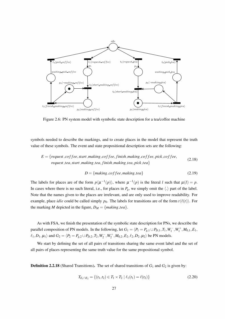
Figure 2.6: PN system model with symbolic state description for a tea/coffee machine

symbols needed to describe the markings, and to create places in the model that represent the truth

value of these symbols. The event and state propositional description sets are the following:

E = {request co f f ee,start making co f f ee, f inish making co f f ee, pick co f f ee,

request tea,start making tea, f inish making tea, pick tea}(2.18)

D = {making co f f ee,making tea} (2.19)

The labels for places are of the form p〈µ−1(p)〉, where µ−1(p) is the literal l such that µ(l) = p.

In cases where there is no such literal, i.e., for places in Pg, we simply omit the 〈.〉 part of the label.

Note that the names given to the places are irrelevant, and are only used to improve readability. For

example, place idle could be called simply p0. The labels for transitions are of the form t〈`(t)〉. For

the marking M depicted in the figure, DM = {making tea}.

As with FSA, we finish the presentation of the symbolic state description for PNs, we describe the

parallel composition of PN models. In the following, let G1 = 〈P1 = Pg,1∪PD,1,T1,W−1 ,W+1 ,M0,1,E1,

`1,D1,µ1〉 and G2 = 〈P2 = Pg,2∪PD,2,T2,W−2 ,W+2 ,M0,2,E2, `2,D2,µ2〉 be PN models.

We start by defining the set of all pairs of transitions sharing the same event label and the set of

all pairs of places representing the same truth value for the same propositional symbol.

Definition 2.2.18 (Shared Transitions). The set of shared transitions of G1 and G2 is given by:

TE1∩E2 = {(t1, t2) ∈ T1×T2 | `1(t1) = `(t2)} (2.20)

27

Definition 2.2.19 (Shared Places). The set of shared places of G1 and G2 is given by:

PD1∩D2 =⋃

d∈D1∩D2

{(µ1(d),µ2(d)), (µ1(¬d),µ2(¬d))} (2.21)

Definition 2.2.20 (Non-Conflicting Petri Net Models). G1 and G2 are said to be non-conflicting if

they satisfy the following statements:

• P1∩P2 = /0;

• T1∩T2 = /0;

• The initial markings assign the same truth value to the propositional symbols in D1∩D2:

For all (p1, p2) ∈ PD1∩D2 , M0,1(p1) = M0,2(p2) (2.22)

• Transition pairs in TE1∩E2 assign the same truth value to the propositional symbols in D1∩D2:

For all (t1, t2) ∈ TE1∩E2 and (p1, p2) ∈ PD1∩D2 , W+1 (p1, t1) =W+

2 (p2, t2) (2.23)

To guarantee that we are able to soundly define the literals corresponding to shared places, we

need to assume that G1 and G2 are non-conflicting, i.e., the firing of shared events in G1 and G2 yields

the same truth value for the shared state description symbols of both nets. The parallel composition

G1 ‖ G2 of G1 and G2 is obtained by simply connecting both models through the merging of pairs

of transitions (t1, t2) ∈ TE1∩E2 and the pairs of places (p1, p2) ∈ PD1∩D2 , while keeping the arc-weight

functions of G1 and G2. Note that this notion of parallel composition is not exactly the same as the

classical one, which is based on merging only transitions with the same event label. In our case, we

also merge places, which can cause tokens to move from one net to the other. This makes it harder to

give an algebraic description of the meaning of the composition, but its intuitive meaning is simple:

places that represent the same environment variable are fused. Furthermore, given the restrictions in

Definition 2.2.20, the places in PD will continue to have 1 or 0 tokens in all reachable markings of the

resulting PN.

Definition 2.2.21 (Parallel Composition). The parallel composition of G1 and G2 is the PN model

G1 ‖ G2 = 〈P1‖2,T1‖2,W−1‖2,W

+1‖2,M0,1‖2,E1∪E2, `1‖2,D1∪D2,µ1‖2〉, where:

• P1‖2 = Pg,1‖2∪PD,1‖2 is the union of non-shared places of G1 and G2 with the pairs representing

the shared places, i.e., Pg,1‖2 = Pg,1∪Pg,2 and PD,1‖2 = PD1\D2 ∪PD2\D1 ∪PD1∩D2 , where:

PD1\D2 = {p ∈ PD1 | p = µ1(d) or p = µ1(¬d), with d ∈ D1 \D2} (2.24)

PD2\D1 = {p ∈ PD2 | p = µ2(d) or p = µ2(¬d), with d ∈ D2 \D1} (2.25)

28

• T1‖2 is the union of the non-shared transitions of G1 and G2 with the pairs representing the

shared transitions, i.e., T1‖2 = TE1\E2 ∪TE2\E1 ∪TE1∩E2 , where:

TE1\E2 = {t ∈ T1 | `1(t) ∈ E1 \E2} (2.26)

TE2\E1 = {t ∈ T2 | `2(t) ∈ E2 \E1} (2.27)

• W−1‖2 ∈N|P1‖2|×|T1‖2| maintains the same arc weights as W−1 and W−2 , taking into account that the

shared places and shared transitions of G1 and G2 are now merged into a single place and a

single transition, respectively:

W−1‖2(p, t) =

W−1 (p, t) if t ∈ TE1\E2 and p ∈ PD1\D2

W−2 (p, t) if t ∈ TE2\E1 and p ∈ PD2\D1

W−1 (p, t1) if t = (t1, t2) ∈ TE1∩E2 and p ∈ PD1\D2

W−2 (p, t2) if t = (t1, t2) ∈ TE1∩E2 and p ∈ PD2\D1

W−1 (p1, t) if t ∈ TE1\E2 and p = (p1, p2) ∈ PD1∩D2

W−2 (p2, t) if t ∈ TE2\E1 and p = (p1, p2) ∈ PD1∩D2

W−1 (p1, t1) =W−2 (p2, t2) if t = (t1, t2) ∈ TE1∩E2 and p = (p1, p2) ∈ PD1∩D2

0 otherwise(2.28)

Note that, for t = (t1, t2) ∈ TE1∩E2 and p = (p1, p2) ∈ PD1∩D2 , we have the guarantee that

W−1 (p1, t1) = W−2 (p2, t2) because the PN models are assumed to be non-conflicting. Through-

out the rest of the definition we will continue to explicitly state the equalities that stem from

this assumption in order to clarify the reader where the non-conflicting assumption is required

for a sound definition of parallel composition.

• W+1‖2 ∈ N|P1‖2|×|T1‖2| is defined analogously to W−1‖2:

W+1‖2(p, t) =

W+1 (p, t) if t ∈ TE1\E2 and p ∈ PD1\D2

W+2 (p, t) if t ∈ TE2\E1 and p ∈ PD2\D1

W+1 (p, t1) if t = (t1, t2) ∈ TE1∩E2 and p ∈ PD1\D2

W+2 (p, t2) if t = (t1, t2) ∈ TE1∩E2 and p ∈ PD2\D1

W+1 (p1, t) if t ∈ TE1\E2 and p = (p1, p2) ∈ PD1∩D2

W+2 (p2, t) if t ∈ TE2\E1 and p = (p1, p2) ∈ PD1∩D2

W+1 (p1, t1) =W+

2 (p2, t2) if t = (t1, t2) ∈ TE1∩E2 and p = (p1, p2) ∈ PD1∩D2

0 otherwise(2.29)

• M0,1‖2 : P1‖2 → N maintains the respective initial markings of G1 and G2, taking into account

29

the merging of shared places:

M0,1‖2(p) =

M0,1(p) if p ∈ PD1\D2

M0,2(p) if p ∈ PD2\D1

M0,1(p1) = M0,2(p2) if p = (p1, p2) ∈ PD1∩D2

(2.30)

• `1‖2 : T1‖2→ E1∪E2 maintains the respective transition labels of G1 and G2, taking into account

the merging of shared transitions:

`1‖2(t) =

`1(t) if t ∈ TE1\E2

`2(t) if t ∈ TE2\E1

`1(t1) = `2(t2) if t = (t1, t2) ∈ TT1∩T2

(2.31)

• µ1‖2 : lit(D1 ∪D2)→ PD1‖2 maintains the relations between places and truth values of state

description symbols of G1 and G2, taking into account the merging of shared places:

µ1‖2(d) =

µ1(d) if d ∈ D1 \D2

µ2(d) if d ∈ D2 \D1

(µ1(d),µ2(d)) if d ∈ D1∩D2

(2.32)

µ1‖2(¬d) =

µ1(¬d) if d ∈ D1 \D2

µ2(¬d) if d ∈ D2 \D1

(µ1(¬d),µ2(¬d)) if d ∈ D1∩D2

(2.33)

The parallel composition simply models the simultaneous execution of G1 and G2, where common

events are synchronized, i.e., a common event can only be executed if both G1 and G2 can execute

it simultaneously. We also merge the places that correspond to the same truth value of the same

propositional symbol, since they represent the same information. We will use the parallel composition

on the PN models of different modules of the same system, thus obtaining the PN model for the

simultaneous execution of all modules11.

Example 2.2.3 (Two Robots Moving a Bar). In Figures 2.7 and 2.8, we show two PN system models

G1 and G2 for robots that are able to grab a bar and move it. Due to the length of the bar, it can only be

moved if each robot grabs one of the bar ends. Each of the models contain the actions available to the

corresponding robots, and the places describing the state of the robot (if it is holding the bar) and the

state of the bar (which sides of the bar are being held, and if the bar is moving). The move bar action

is a shared action which abstracts the coordination needed to perform the actual movement. Hence,

these models have both shared events and shared state description symbols. We list the sets used in

11Note that in the case of multi-robot systems which we will focus on for the application of our methodology, we can useparallel composition on models of different possible behaviours for a given single robot and also on the individual modelsof a team of robots. This will be exemplified on Section 6.3.

30

Figure 2.7: PN model for robot 1

the parallel composition definition for this specific case:

• PD1\D2 = {p11, p2

1};

• PD2\D1 = {p12, p2

2};

• PD1∩D2 = {(p31, p3

2),(p41, p4

2),(p51, p5

2),(p61, p6

2),(p71, p7

2),(p81, p8

2)};

• TE1\E2 = {t11 , t

21};

• TE2\E1 = {t12 , t

22};

• TE1∩E2 = {(t31 , t

32)}.

In Figure 2.9, we depict the PN system model for the whole system, which is obtained by the

parallel composition of the robot models. Note that the shared places and shared transitions were

merged, but both the initial markings and the arc weights of G1 and G2 are maintained. Thus, the

substructures of G1 and G2 are clearly represented in the output of the composition.

2.2.2 Linear Algebraic State Description

When using the symbolic state representation, we do not take into direct account the fact that the PN

state can be represented algebraically. This fact will enable us to enrich and shorten our specifications

as we will see when discussing the LTL semantics for this approach.

31

Figure 2.8: PN model for robot 2

Figure 2.9: PN representing the composition of 2.7 and 2.8

32

Definition 2.2.22 (Petri Net System Model – Linear Algebraic State Description). A Petri net system

model is a tuple G = 〈L,κ, 〉 where:

• L = 〈P,T,W−,W+,M0,E, `〉 is a labelled PN where P = Pb∪Pω , with Pb∩Pω = /0;

• κ : Pb→ N is the maximum token function where, for all p ∈ Pb and M ∈ R(G):

– M(p)≤ κ(p).

• : Pb→Pb is the complement place function, where , for all p∈Pb, p satisfies Definition 2.2.13.

The places p ∈ Pb are places for which the designer knows a bound κ(p). We also define a com-

plement function that associates each place in Pb to a complement place. As explained previously, for

bounded places that do not have a complement place in the PN structure, we can add the complement

place without changing the modelled behaviour, by using the construction in Definition 2.2.14. Note

that this bound can be obtained by using analysis techniques and that it is not necessarily strict: κ(p)

can be strictly greater than M(p) for all M ∈ R(G). Places p ∈ Pω are either (i) unbounded places or

(ii) bounded places for which the designer does not know the bound.

Remark 2.2.1. Note that PN system models with symbolic state representation are subsumed in PN

system models with algebraic state representation. To see this, consider the PN system model with

symbolic state representation Gsymb = 〈L,D,µ〉. It can be modelled as the PN system model with

algebraic state representation Galg = 〈L,κ, 〉, where:

• Pb = PD;

• Pω = Pg;

• κ(p) = 1 for all p ∈ Pb;

• For all p, p′ ∈ Pb, p = p′ if and only if exists d ∈ D such that µ(d) = p and µ(¬d) = p′ or

µ(d) = p′ and µ(¬d) = p.

Example 2.2.4 (Tea/Coffee Machine). In Figure 2.10 we depict the algebraic state description version

of the PN with symbolic state description for a tea and coffee machine depicted in Figure 2.6. We

also add a limit to the number of teas and coffees that can be served before the machine needs to be

refilled. We assume that the machine can only hold 20 doses of coffee and 20 doses of tea.

The labels for the transitions are depicted as t〈`(t)〉, as before. For the places, we directly depict

the complement function when it is defined. Note that, for example, making tea = making tea. For

the place bounds, we have the following:

• κ(making tea) = κ(making tea) = 1;

• κ(making co f f ee) = κ(making co f f ee) = 1;

• κ(n f ull slots tea) = κ(n f ull slots tea) = 20;

33

Figure 2.10: PN system model with algebraic state description for a tea/coffee machine

• κ(n f ull slots co f f ee) = κ(n f ull slots co f f ee) = 20;

Note that, for example place waiting pick co f f ee does not have a complement place depicted.

However, since κ(waiting pick co f f ee) = 1, we can add its complement place without changing the

modelled behaviour, as explained before.

We finish by describing the parallel composition for PN models with algebraic state descriptions.

In the following, let Gi =⟨Pi = Pb,i∪Pω,i,Ti,W−i ,W+

i ,M0,i,Ei, `i,κi,i⟩, i = 1,2 be PN system mod-

els.

The set of shared transitions is defined as before (see Definition 2.2.18), but in this case we do not

need to define the set of shared places from the state description symbols.

Definition 2.2.23 (Non-Conflicting Petri Net Models). G1 and G2 are said to be non-conflicting if

they satisfy the following statements:

• T1∩T2 = /0;

• The initial markings assign the same truth value to places in P1∩P2:

For all p ∈ P1∩P2, M0,1(p) = M0,2(p) (2.34)

• Transition pairs in TE1∩E2 have coincident pre and post sets for places p ∈ P1∩P2:

For all (t1, t2) ∈ TE1∩E2 and p ∈ P1∩P2, W−1 (p, t1) =W−2 (p, t2) and W+1 (p, t1) =W+

2 (p, t2)

(2.35)

34

• Places in P1∩P2 have the same bound and the same complement place:

For all p ∈ P1∩P2, κ1(p) = κ2(p) and p1 = p2 (2.36)

Note that, in this case, we do not assume that P1 ∩P2 = /0. This is because, in this case, we use

P1 and P2 to identify shared places, instead of D1 and D2, which were used in the symbolic state

representation case. As for the PN models with symbolical state descriptions, we need to assume

that G1 and G2 are non-conflicting so that the parallel composition is well-defined. We note that the

idea for this parallel composition is exactly the same as the one defined for PN system models with

symbolic state description, the main reason to include it here is to keep both subsections self-contained

and explicitly state the small adaptations needed.

Definition 2.2.24 (Parallel Composition). The parallel composition of G1 and G2 is the PN model

G1 ‖ G2 = 〈P1∪P2,T1‖2,W−1‖2,W

+1‖2,M0,1‖2,E1∪E2, `1‖2,κ1‖2,

1‖2〉, where:

• T1‖2 is the union of the non-shared transitions of G1 and G2 with the pairs representing the

shared transitions, i.e., T1‖2 = TE1\E2 ∪TE2\E1 ∪TE1∩E2 , where:

TE1\E2 = {t ∈ T1 | `1(t) ∈ E1 \E2} (2.37)

TE2\E1 = {t ∈ T2 | `2(t) ∈ E2 \E1} (2.38)

• W−1‖2 ∈N|P1‖2|×|T1‖2| maintains the same arc weights as W−1 and W−2 , taking into account that the

shared places and shared transitions of G1 and G2 are now merged into a single place and a

single transition, respectively:

W−1‖2(p, t) =

W−1 (p, t) if t ∈ TE1\E2 and p ∈ P1 \P2

W−2 (p, t) if t ∈ TE2\E1 and p ∈ P2 \P1

W−1 (p, t1) if t = (t1, t2) ∈ TE1∩E2 and p ∈ P1 \P2

W−2 (p, t2) if t = (t1, t2) ∈ TE1∩E2 and p ∈ P2 \P1

W−1 (p, t) if t ∈ TE1\E2 and p ∈ P1∩P2

W−2 (p, t) if t ∈ TE2\E1 and p ∈ P1∩P2

W−1 (p, t1) =W−2 (p, t2) if t = (t1, t2) ∈ TE1∩E2 and p ∈ P1∩P2

0 otherwise

(2.39)

Note that, for t = (t1, t2) ∈ TE1∩E2 and p ∈ P1 ∩ P2, we have the guarantee that

W−1 (p1, t1) = W−2 (p2, t2) because the PN models are assumed to be non-conflicting. Through-

out the rest of the definition we will continue to explicitly state the equalities that stem from

this assumption in order to clarify the reader where the non-conflicting assumption is required

for a sound definition of parallel composition.

35

• W+1‖2 ∈ N|P1‖2|×|T1‖2| is defined analogously to W−1‖2:

W+1‖2(p, t) =

W+1 (p, t) if t ∈ TE1\E2 and p ∈ P1 \P2

W+2 (p, t) if t ∈ TE2\E1 and p ∈ P2 \P1

W+1 (p, t1) if t = (t1, t2) ∈ TE1∩E2 and p ∈ P1 \P2

W+2 (p, t2) if t = (t1, t2) ∈ TE1∩E2 and p ∈ P2 \P1

W+1 (p, t) if t ∈ TE1\E2 and p ∈ P1∩P2

W+2 (p, t) if t ∈ TE2\E1 and p ∈ P1∩P2

W+1 (p, t1) =W+

2 (p, t2) if t = (t1, t2) ∈ TE1∩E2 and p ∈ P1∩P2

0 otherwise

(2.40)

• M0,1‖2 : P1‖2 → N maintains the respective initial markings of G1 and G2, taking into account

the merging of shared places:

M0,1‖2(p) =

M0,1(p) if p ∈ P1

M0,2(p) if p ∈ P2

M0,1(p) = M0,2(p) if p ∈ P1∩P2

(2.41)

• `1‖2 : T1‖2→ E1∪E2 maintains the respective transition labels of G1 and G2, taking into account

the merging of shared transitions:

`1‖2(t) =

`1(t) if t ∈ TE1\E2

`2(t) if t ∈ TE2\E1

`1(t1) = `2(t2) if t = (t1, t2) ∈ TT1∩T2

(2.42)

• κ1‖2 : P1∪P2→ N maintains the bounds for all places:

κ1‖2(p) =

κ1(p) if p ∈ P1 \P2

κ2(p) if p ∈ P2 \P1

κ1(p) = κ2(p) if p ∈ P1∩P2

(2.43)

• 1‖2 : Pb,1∪Pb,2→ Pb,1∪Pb,2 maintains the complement places for all places:

p1‖2 =

p1 if p ∈ Pb,1 \Pb,2

p2 if p ∈ Pb,2 \Pb,1

p1 = p2 if p ∈ Pb,1∩Pb,2

(2.44)

The parallel composition simply models the simultaneous execution of G1 and G2, where common

events are synchronized, i.e., a common event can only be executed if both G1 and G2 can execute it

simultaneously. We also merge the places that are equal.

36

Example 2.2.5. Consider Figure 2.11, which depicts the model Gi of the connection and team choice

of player i, i ∈ {1,2,3,4} to an online 2 versus 2 card playing game. The player starts by connecting

to the game server, and, once it is connected it chooses whether he wants to be part of team 1 or team

2. Transitions t5i correspond to starting the game and are all labelled by the same event in all models,

hence they are shared and need to be synchronized. Furthermore, places n team1, n team1, n team2,

n team2 and game started are also shared by all the player models, so they are merged. These places

represent global variables of the system. Thus, the sets used in the parallel definition composition of,

for example, G1 and G2, are the following:

• P1 \P2 = {idle1,connecting to game1, in game1};

• P2 \P1 = {idle2,connecting to game2, in game2};

• P1∩P2 = {n team1,n team1,n team2,n team2,game started};

• TE1\E2 = {t11 , t

21 , t

31 , t

41};

• TE2\E1 = {t12 , t

22 , t

32 , t

42};

• TE1∩E2 = {(t51 , t

52)}.

Figure 2.12 depicts the model G = G1 ‖ G2 ‖ G3 ‖ G4 of the whole player connection and team

choices, obtained by the parallel composition of the 4 player models. Note that in the team model,

only 2 players can choose to be in a given team, given that we merged the places corresponding to

the shared resources n team1 and n team2. This example also illustrates the scalability of the parallel

composition for PNs when compared to the parallel composition for FSA: The substructure of each

of the four subsystems is clearly identifiable in the result of their parallel composition, given that only

some places and transitions were merged, while in the case of FSA parallel composition, the states

of the composition would represent the Cartesian product of states in each of the subsystems, thus

growing much more rapidly.

37

Figure 2.11: Petri net model of a card player

38

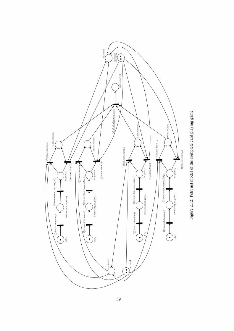
Figu

re2.

12:P

etri

netm

odel

ofth

eco

mpl

ete

card

play

ing

gam

e

39

CHAPTER 3

Specification Language

In this chapter, we present the concepts of formal logic and formal languages that will be used through-

out the work. We start by providing the basics of linear temporal logic (LTL), its semantics over the

basic models defined in the previous chapter, and its translation to Buchi automata (BA). Afterwards,

we will discuss the notion of safety languages and restrict the specification language to safe LTL for-

mulas, providing a discussion on the expressiveness of this type of specification. In the following, let

Π be a countable set of atomic propositions and (2Π)ω the set of all infinite sequences of subsets of

Π.

3.1 Linear Temporal Logic

In this section we will briefly define linear temporal logic (LTL) and describe its semantics over the

system models we presented. Furthermore, we will describe the translation of LTL to Buchi automata,

which is a crucial step in our methodology, given that the fact that we can have an automata-theoretic

view of LTL formulas is what allows us to then proceed with the restriction of the system models so

that they satisfy a formula. LTL is an extension of propositional logic which allows reasoning over an

infinite sequence of states. It was developed as a formal verification tool for concurrent systems, as it

provides a close-to-natural-language way to specify and verify qualitative properties of a system.

3.1.1 Syntax and Semantics over the System Models

Definition 3.1.1 (Syntax). An LTL formula over a set Π of atomic propositions has the following

syntax:

• true, f alse and π ∈Π are LTL formulas;

41

• If ϕ and ψ are LTL formulas then (¬ϕ), (ϕ ∨ψ), (Xϕ), (ϕUψ) and (ϕRψ) are also LTL

formulas.

LTL formulas are evaluated over infinite sequences of sets of propositional symbols

σ = σ0σ1σ2... ∈ (2Π)ω , i.e., σi ∈ 2Π for i ∈ N. The logical operators will have the same seman-

tics for all the models, but we will have different ways of evaluating atomic propositions, depending

on the model we are using. Thus, we start by giving the usual definition of satisfaction for LTL and a

generic set of atomic propositions Π, and then discuss how the satisfaction of atomic propositions is

specialized to the system models.

Definition 3.1.2 (Satisfaction). Let σ ∈ (2Π)ω , t ∈ N. The notion of local satisfaction, , is defined

as follows:

• σt true and σt 6 f alse;

• σt π if and only if π ∈ σt ;

• σt (¬ϕ) if and only if σt 6 ϕ;

• σt (ϕ ∨ψ) if and only if σt ϕ or σt ψ;

• σt (ϕ ∧ψ) if and only if σt ϕ and σt ψ;

• σt (Xϕ) if and only if σt+1 ϕ;

• σt (ϕUψ) if and only if there exists t ′ ≥ t such that σt ′ ψ and for all t ′′ ∈ [t, t ′[ σt ′′ ϕ;

• σt (ϕRψ) if and only if for all t ′ ≥ t, if σt ′ ψ then there exists t ′′ ∈ [t, t ′[ such that σt ′′ ϕ;

If σ0 ϕ we say that σ (globally) satisfies ϕ , which is simply written σ ϕ .

The propositional fragment of LTL, i.e., formulas written without the temporal operators X , U and

R, is evaluated only over one element σt ∈ 2Π of σ ∈ (2Π)ω . Hence, when evaluating propositional

formulas ϕ , we will sometimes use the notation S ϕ , where S ∈ 2Π.

The temporal operators are understood as follows:

• The X operator is read “next”, meaning that the formula it precedes will be true in the next state.

• The U operator is read “until”, meaning that its first argument will be true until its second argu-

ment becomes true (and the second argument must become true in some state, i.e., a sequence

where ϕ is always satisfied but ψ is never satisfied does not satisfy ϕUψ).

• The R operator is read “release”, meaning that its second argument can only become true if its

first argument became true before (i.e., the occurrence of the first argument releases the need

for the second argument to be true). For this operator, if the first argument never becomes true,

the second argument must remain true for all times.

42

We will now instantiate the set of propositional symbols to the system model being used.

Definition 3.1.3 (Atomic Propositions – System Models). Let G be a system model. The set of atomic

propositions is defined as:

• Πsymb = D ∪ E if G = 〈Q,E,δ ,q0,D,µ〉 is an FSA system model or

G = 〈PD∪Pg,T,W−,W+,M0,E, `,D,µ〉 is a PN system model with symbolic state description.

• Πalg = (Pb ×N)∪ E if G = 〈Pb ∪ Pω ,T,W−,W+,M0,E, `,κ, 〉 is a PN system model with

algebraic state description.

Intuitively, an element (p,b) of Πalg means that the number of tokens in place p should be greater

or equal than b. Thus, to facilitate the comprehension, when presenting formulas we will write the

elements (p,b) of Πalg as M(p)≥ b, b ∈ N.

Given that the languages generated by the system models are infinite sequences of event/state

pairs, and our goal is to restrict these languages using LTL, we need to define what subset of atomic

propositions these pairs represent, so that we can evaluate LTL formulas over the languages generated

by the systems.

Definition 3.1.4 (Event/State Semantics – FSA). Let G= 〈Q,E,δ ,q0,D,µ〉 be an FSA system model,

q ∈ Q, e ∈ E. The pair (e,q) generates the set {e}∪µ(q) ∈ 2Πsymb .

Definition 3.1.5 (Event/Marking Semantics – PN with Symbolic State Representation). Let G =

〈P,T,W,M0,E, `,D,µ〉 be an PN system model with symbolic state representation, M ∈ R(G), e ∈ E.

The pair (e,M) generates the set {e}∪DM ∈ 2Πsymb .

Definition 3.1.6 (Event/Marking Semantics – PN with Algebraic State Representation). Let G =

〈P,T,W−,W+,M0,E, `,κ, 〉 be an PN system model with algebraic state representation, M ∈ R(G),

e ∈ E. The pair (e,M) generates the set {e}∪{(p,b) ∈ Pb×N |M(p)≥ b} ∈ 2Πalg .

Note that, to check if a given pair (p,b) is in the set generated by (M,e), we just need to check if

M(p) ≥ b is a true statement. We will slightly abuse the notation and, given an element σ ∈L (G),

i.e., an infinite sequence of event/state pairs, we will write σ ϕ if the infinite sequence composed of

the sets generated by the event/state pairs in σ satisfies ϕ , according to Definition 3.1.2.

For PN system models with algebraic state representation, we only consider linear constraints of

the form M(p) ≥ b with p ∈ P and b ∈ N in this semantics. In spite of that, this already gives us a

good amount of expressibility, since any constraint consisting of linear combinations of the number

of tokens in the bounded places of a PN can be re-written in this form, as we will show later.

The more attentive reader might have noticed that we are using the ∧ and R operators, which are

not fundamental operators, in the sense that any LTL formula can be written using only the other

operators. This of because if the identities (ϕ ∧ψ) = (¬(¬ϕ ∨¬ψ)) and (ϕRψ) = (¬(¬ϕU¬ψ)).

However, ∧ and R are required to write formulas in the so called positive normal form (PNF), where

only atomic propositions can be negated. As will be discussed later, we will write all our formulas in

the PNF, so we can syntactically ensure that we are writing safety formulas.

43

Definition 3.1.7 (Positive Normal Form). An LTL formula over Π in the positive normal form (PNF)

has the following syntax:

• true, f alse, π and ¬π , with π ∈Π are LTL formulas in the PNF;

• If ϕ and ψ are LTL formulas in the PNF then (ϕ ∨ψ), (Xϕ), (ϕUψ) and (ϕRψ) are also LTL

formulas in the PNF.

Using the following identities, one can convert any LTL formula to the PNF:

• (¬true) = f alse and (¬ f alse) = true;

• (¬(¬ϕ)) = ϕ;

• (¬(ϕ ∧ψ)) = (¬ϕ ∨¬ψ) and (¬(ϕ ∨ψ)) = (¬ϕ ∧¬ψ);

• (¬Xϕ) = (X¬ϕ);

• (¬(ϕUψ)) = (¬ϕR¬ψ) and (¬(ϕRψ)) = (¬ϕU¬ψ).

Hence, we do not lose expressiveness by using the PNF.

Example 3.1.1. We provide an example of conversion of an LTL formula to the PNF:

¬(((Xπ1)U(¬(π2R¬π3)))∧ (trueU¬π2)) = ¬((Xπ1)U(¬(π2R¬π3)))∨¬(trueU¬π2)

= (¬Xπ1)R(¬¬(π2R¬π3))∨ f alseRπ2

= (X¬π1)R(π2R¬π3)∨ f alseRπ2

In addition to the usual propositional logic abbreviations, there are other temporal operators usu-

ally also defined by abbreviation.

Definition 3.1.8 (Abbreviations). We define the following abbreviations:

• (ϕ ⇒ ψ)≡abv ((¬ϕ)∨ψ);

• (ϕ ⇔ ψ)≡abv ((ϕ ⇒ ψ)∧ (ψ ⇒ ϕ));

• (Fϕ)≡abv (trueUϕ);

• (Gϕ)≡abv ( f alseRϕ) = (¬F(¬ϕ));

• (ϕWψ)≡abv ((ϕUψ)∨ (Gϕ)) = (ψR(ψ ∨ϕ)).

The temporal abbreviations are understood as follows:

• The F operator is read “eventually” and requires the existence of a future state where the for-

mula it precedes is true.

44

• The G operator is read “always” and requires the formula it precedes to be true in all future

states.

• The W operator is read “weak until” and relaxes the U operator by allowing its second argument

to never be satisfied.

Example 3.1.2 (Writing LTL formulas). The natural language specification “Whenever the robot

starts moving, it should not stop until it reaches the goal region” can be written as an LTL formula

over the set Πsymb = {start moving, stop moving, goal reached}:

G(start moving⇒ (X(¬stop movingUgoal reached))) (3.1)

The natural language specification “In all markings, if the number of tokens in place p1 is greater

or equal than 2 then, in the next marking, either the marking in place p2 is greater or equal than 4 or

event put token in p2 just occurred:

G((p1,2)⇒ (X((p2,4)∨ put token in p2))) (3.2)

As we already mentioned, when writing formulas, we will replace atomic propositions (p,b) by

M(p)≥ b in order to improve readability,. Hence, the specification can be re-written as:

G(M(p1)≥ 2⇒ (X(M(p2)≥ 4∨ put token in p2))) (3.3)

3.1.2 Translation to Buchi automata

We now present Buchi automata (BA), which will be used as a representation of an LTL formula. A

BA is a finite state automaton equipped with the so called Buchi acceptance condition. We start by

noting that LTL formulas can be used to generate ω-languages.

Definition 3.1.9 (Language generated by an LTL formula). Let ϕ be an LTL formula. The ω-language

generated by ϕ is given by:

L (ϕ) = {σ ∈ (2Π)ω | σ ϕ} (3.4)

We designate the class of languages generated by LTL formulas as LTL languages.

Example 3.1.3. We provide examples on the languages generated by LTL formulas:

• L (Fπ1) = {σ = σ0σ1... ∈ (2Π)ω | exists t ∈ N such that π1 ∈ σt}. For example, any ω-string

with the prefix {π0}{π0,π2,π3} /0{π0,π1}{π2} is part of L (Fπ1), because π1 ∈ σ3.

• L (Gπ1) = {σ = σ0σ1... ∈ (2Π)ω | for all t ∈ N, π1 ∈ σt}. For example, the ω-string

{π1}{π0,π1}{π1,π2}{π1}{π1}{π1}... is part of L (Gπ1) (assuming that π1 occurs in all the

other states of the ω-string).

45

• L (FGπ1) = {σ =σ0σ1...∈ (2Π)ω | exists t ∈N such that for all t ′≥ t, π1 ∈σt ′}. For example,

the ω-string {π0}{π3}{π0,π1}{π0} /0{π1,π2}{π1,π2}{π1,π2}... is part of L (FGπ1) (assuming

that π1 occurs in all the other states of the ω-string).

Hence, we are interested in finding another way to represent the language generated by an LTL

formula, which is more related to our system models. The structure we will use to represent LTL

languages will be Buchi automata, for which translation algorithms from LTL formulas have been

widely studied.

Definition 3.1.10 (Buchi Automaton). A Buchi automaton (BA) is a tuple B = 〈Q,Σ,δ ,Q0,QF〉where:

• 〈Q,Σ,δ ,Q0〉 is a (non-deterministic) FSA.

• QF ⊆ Q is the set of accepting states.

In order to define the accepted ω-language by a BA, we introduce valid state labellings.

Definition 3.1.11 (Valid State Labelling). Let B = 〈Q,Σ,δ ,Q0,QF〉 and σ ∈ Σω . A valid state la-

belling for B and σ is an infinite sequence ρ ∈ Qω such that:

ρ0 ∈ Q0 (3.5)

ρi+1 ∈ δ (ρi,σi) for all i ∈ N (3.6)

We denote P(B,σ) as the set of all possible valid state labellings for B and σ .

A valid state labelling for B and σ is an infinite sequence of states that are visited in a “run” of B

while following σ . P(B,σ) can be empty if σ does not respect the transition function δ or can have

one or more elements due to the non-determinism of the automaton.

Definition 3.1.12 (Language Accepted by a Buchi Automaton). The ω-language accepted by a BA

B = 〈Q,Σ,δ ,Q0,QF〉 is defined as follows:

L (B) = {σ ∈ Σω | exists ρ ∈ P(B,σ) such that in f (ρ)∩QF 6= /0} (3.7)

For ρ ∈ Qω , in f (ρ) is the set of all q ∈ Q that appear infinite times in ρ . The class of languages

accepted by Buchi automata is the class of ω-regular languages.

The accepted ω-strings by B are the ones that correspond to at least one run of B that visits at least

one of the accepting states infinite times. The following proposition states the relation between BA

and LTL formulas.

Proposition 3.1.1 ( [Wolper, 2001]). Let ϕ be an LTL formula written over Π. Then there exists a

(non-deterministic) BA Bϕ = 〈Q,2Π,δ ,q0,QF〉 such that L (Bϕ) = L (ϕ).

46

There are several methods for the construction of this automaton. In the implementation of the

method we present here, we use one of the most efficient translation algorithms, LTL2BA, described

in [Gastin and Oddoux, 2001]. In the BA obtained by applying the LTL2BA algorithm, propositional

formulas in the disjunctive normal form (DNF) are used to describe the transition labels in a more

compact way. A formula is in the DNF if it is of the form:

n∨i=1

mi∧j=i

li j, where li j ∈ lit(Π) (3.8)

The elements∧mi

j=i li j are called conjunctive clauses. In words, a conjunctive clause is the conjunction

of a set of literals and a DNF formula is the disjunction of a set of conjunctive clauses. For example,

if ψ1 = (π1 ∧¬π2)∨ (π3) is a transition label, then all elements of 2Π that contain π1 and do not

contain π2, or that contain π3 are labels of that transition, i.e., it represents the set of transition labels

{S ∈ 2Π | π1 ∈ S and π2 6∈ S}∪{S ∈ 2Π | π3 ∈ S}. The label true is also used, to represent the set of all

possible transition labels, i.e., to represent that any subset of Π can occur. Given an element S ∈ 2Π

and a DNF formula ψ written over Π, the easiest way to check if S is one of the transition labels coded

by ψ is to check if S ψ , using the notions of satisfaction for the propositional connectives ¬, ∧ and

∨ and for the atomic propositions we presented. Note that this is the propositional fragment of LTL,

hence we only need one element of an infinite string to evaluate them.

Example 3.1.4 (Evaluating DNF Labels). Given S = {π1,π3}, ψ1 = (π1 ∧¬π2)∨ (π3) and ψ2 =

(π1∧π2)∨ (¬π2∧¬π3), we have the following:

• S ψ1, because both π1 ∈ S and π2 6∈ S, and π3 ∈ S. Hence, both conjunctive clauses are

satisfied, thus so is the DNF formula. Note that satisfying one of the conjunctive clauses would

suffice.

• S 6 ψ2, because, for the first conjunctive clause, π2 6∈ S and, for the second conjunctive clause

π3 ∈ S. Hence, both conjunctive clauses are not satisfied, and neither is the DNF formula.

Given that the labels are written in the DNF and a DNF formula is satisfied if and only if at least

one of its conjunctive clauses are satisfied, it is easy to check if a given subset of 2Π satisfies the

formula, by checking each conjunctive clause until we find one that is satisfied, or we conclude that

none of the conjunctive clauses in the DNF formula are satisfied. Furthermore, any propositional

formula can be rewritten in the DNF and, given an arbitrary propositional formula ψ , we will write

DNF(ψ) to denote the DNF representation of ψ .

Example 3.1.5 (A Buchi Automaton). Figure 3.1 depicts the BA obtained by using LTL2BA for

formula :

G(start moving⇒ (X(¬stop movingUgoal reached))) (3.9)

The label true means that any symbol from the alphabet 2Π can drive the automaton from state

1 to state 2. Hence, any symbol (i.e., any subset of {start moving,stop moving,goal reached} that

47

Figure 3.1: BA obtained from G(start moving⇒ (X(¬stop movingUgoal reached)))

Figure 3.2: BA accepting L = {σ ∈ (2Π)ω | π ∈ σ2i, i ∈ N}

does not contain start moving will correspond to a non-deterministic transition, where the automaton

can go to both state 1 or 2 (it satisfies both transition label true and transition label ¬start moving).

State 1 is the initial state, and states 1 and 3 are accepting states, hence any run which visits 1 or 3

infinite times is accepted by the BA.

We also note that the inclusion of LTL languages in ω-regular languages is strict. For example the

language L= {σ ∈ (2Π)ω | π ∈σ2i, i∈N}, i.e., the language of infinite strings where π occurs in every

even index, can be represented by the BA in Figure 3.2. However it is not an LTL language [Wolper,

1983].

We now introduce two operators over BA that will be useful to clarify our discussion.

Definition 3.1.13 (Accessible and Co-Accessible States). Let B = 〈Q,Σ,δ ,Q0,QF〉 be a BA. We

define the sets of:

• Accessible states as Qac ⊆ Q such that there is a path for a state q0 ∈ Q0 to a state qac ∈ Qac.

• Co-accessible states as Qco−ac ⊆ Q such that there is a path for a state qco−ac ∈ Qac to a state

q f ∈ QF .

Definition 3.1.14 (Trim Buchi Automaton). Let B be a BA. We define trim(B) as the automaton

obtained by deleting from B all states that are not accessible or not co-accessible.

It is clear that L (B) = L (trim(B)). We will assume that all our BA are trim.

48

Figure 3.3: Non-deterministic BA accepting the ω-language generated by (FGπ).

Definition 3.1.15 (Closure of a Buchi Automaton). Let B = 〈Q,Σ,δ ,Q0,QF〉 be a BA. We define

cl(B) = 〈Q,Σ,δ ,Q0,Q〉.

We obtain the closure of a BA by simply defining all its states as accepting states. Note that, in

general, it is possible to follow a BA transition function and generate an ω-string that is not accepted

by the BA, i.e., L (B) ⊆ L (cl(B)). For example, in Figure 3.1, the ω-string {start moving} /0 /0...,

can be generated by the depicted BA by following its transition function, but it will keep the BA

indefinitely in the non-accepting state 2, thus the ω-string is not accepted by the BA. In fact, given

a BA where L (B) ⊂L (cl(B)), one needs to find its strongly connected components to be able to

generate ω-strings that visit accepting states infinite times. When L (B) = L (cl(B)) we say that B is

closed.

Another important property of BA is that the class of non-deterministic BA is more expressive

than the class of deterministic BA, i.e., there are non-deterministic BA that accept ω-languages that

cannot be represented by a deterministic BA. In particular, the power-set construction used to build

the deterministic version of a non-deterministic automaton is not valid for BA. An example of an

ω-language that is not accepted by a deterministic BA is the language generated by the LTL formula

(FGπ). The non-deterministic BA accepting this language is depicted in Figure 3.3. Note that the BA

depicted in Figures 3.2 and 3.3 also show that the classes of LTL languages and ω-languages accepted

by deterministic BA are not comparable.

In our case, we want to use a deterministic BA – so that we can have a deterministic supervisor

realization – and also we want to avoid the need of applying search algorithms to the BA, hence we

want to deal with BA B such that L (B) = L (cl(B)). To be able to obtain BA with these properties,

we will restrict the LTL formulas we can use to specify behaviours to the so called safety fragment of

LTL. We will be discussing this next.

3.2 Restricting LTL to Safety Properties

One important classes of ω-languages are safety languages. Intuitively, a safety language specifies a

property that states that something “bad” never happens in the system. Safety languages are associated

with invariants of the system. In this section we will discuss safety languages and the restriction of

LTL to specify only safety languages. In the following, let Σ be an alphabet, Σ∗ the set of all finite

strings composed of elements of Σ and Σω the set of all the infinite strings composed of elements of

Σ.

49

Figure 3.4: Deterministic BA accepting the language generated by (Fπ).

We start by defining the notion of bad prefix.

Definition 3.2.1 (Bad Prefix). Let L ⊆ Σω be an ω-language and s ∈ Σ∗. s is a bad prefix for L if for

all σ ∈ Σω , s.σ 6∈ L, where s.σ ∈ Σω is the concatenation of s and σ .

A bad prefix is a finite string that cannot be extended to an infinite string that is in L. Safety

languages are characterized using this notion.

Definition 3.2.2 (Safety Language). Let L⊆ Σω be an ω-language. L is called a safety language if all

σ 6∈ L have a bad prefix for L.

For a safety language, one can always decide if an infinite string is not in the language by observing

a finite part of it. This fact makes these types of languages especially “well-behaved” regarding the

goals of this work, as we will explain next. One should notice that regular safety languages (i.e.,

safety languages that are accepted by BA) are strictly contained in regular ω-languages. The following

proposition characterizes regular safety languages.

Proposition 3.2.1 ( [Alpern and Schneider, 1987]). Let B be a trim BA. Then L (B) is a safety lan-

guage if and only if L (B) = L (cl(B)).

Informally, this proposition states that for a trim BA that accepts a safety language, all the runs are

accepting, i.e., there are no strongly connected components composed of only non-accepting states.

Furthermore, since the power-set construction can be used for cl(B), by defining all the states of the

deterministic automaton as accepting states, we have the following corollary:

Corollary 3.2.1. Let L be a regular safety language. Then there exists a deterministic BA B such that

L (B) = L.

This corollary means that the class of regular safety languages is contained in the class of ω-

languages accepted by deterministic BA. One can also prove that there are ω-languages accepted by

deterministic BA which are not safety languages. For example, the BA in Figure 3.4, which generates

the ω-language that satisfies the LTL formula (Fπ) is deterministic but does not represent a safety

language. Thus, the inclusion of the class of regular languages in the class of languages accepted by

deterministic BA is strict.

We now focus our attention on LTL formulas that generate safety languages.

Definition 3.2.3 (Safe LTL). Let ϕ be an LTL formula. We say that ϕ is an LTL safety formula if

L (ϕ) is a safety language.

50

Safe LTL is strictly contained in regular safety languages. To see that, the BA in Figure 3.2

represents a safety language that is not representable in LTL. The following corollary is a direct

consequence of the fact that LTL safety formulas generate safety languages.

Corollary 3.2.2. Let ϕ be an LTL safety formula. Then there exists a deterministic and closed BA BDϕ

such that L (BDϕ ) = L (ϕ).

Hence, we have a procedure to go from an LTL safety formula ϕ to a deterministic BA for which

every run is accepting, i.e., satisfies ϕ:

1. Translate ϕ into a BA Bϕ using the LTL2BA tool.

2. Apply the power-set construction to cl(trim(Bϕ)), obtaining BDϕ , where all the sets are accepting

states. Taking into account the discussion above, L (BDϕ ) = L (ϕ).

This procedure has the drawback that the power-set construction is exponential in the size of the

nondeterministic automaton. To mitigate this fact, our composition algorithms will take the non-

deterministic BA as input and determinize it “on-the-fly”, while performing the composition. By

doing so, we only add a new state to the deterministic version of the BA if the synchronized run of the

system with the BA can lead us to that state.

To complete our discussion, we just need to guarantee that our specifications are LTL safety

formulas. Unfortunately, it is proven in [Sistla, 1994] that checking in an LTL formula generates a

safety language is a PSPACE-complete problem. Thus, to avoid checking our specifications for safety,

we will use syntactically safe LTL.

Definition 3.2.4 (Syntactically Safe LTL). An LTL formula is syntactically safe if it is in the PNF and

only the operators X , R, G and W are used.

As expected, given our nomenclature, syntactically safe LTL is a subset of safe LTL.

Proposition 3.2.2 ( [Sistla, 1994]). Let ϕ be a syntactically safe LTL formula. Then L (ϕ) is a safety

language.

From the designer point of view, the class of syntactically safe formulas is the class of interest

when specifying safety properties in LTL. This can be justified because, while LTL formulas where

F and U appear can be safe, this happens by “accident”, in the sense that, in general, these operators

require something to eventually happen. Thus, when a formula using F or U is a safety formula,

it means that these operators are redundant in some way. A simple example of this is the formula

(Gπ)∧ (Fπ), which is clearly a safety formula but contains the F operator. We will require our

specifications to be given as syntactically safe LTL formulas.

To summarize this overview of safety languages and LTL, in Figure 3.5 a Venn diagram of the

different classes of languages we presented. We also refer the interested reader to [Vardi, 1996]

for an introduction to Buchi automata and its properties and to [Kupferman and Vardi, 2001] for an

introduction to model checking safety properties.

51

Figure 3.5: Venn diagram for the classes of ω-languages described in this chapter.

52

CHAPTER 4

Composition of Buchi Automaton with System Models

In this chapter, we present the main algorithms developed in this thesis. These are composition algo-

rithms between the system models presented in Chapter 2 and the Buchi automata obtained from LTL

specifications, using the LTL2BA [Gastin and Oddoux, 2001] tool. The result of these compositions

is a system model whose generated language is the generated language of the unsupervised original

system restricted to the ω-strings that satisfy the specification. This model will be used as a coarse

structure for building the supervisor, since it does not guarantee admissibility and deadlock-freeness,

which are two fundamental notions for a proper supervisor in the Ramadge-Wonham framework [Ra-

madge and Wonham, 1989]. We will see how one can build a supervisor from these structures, using

available approaches in the literature, in the next chapter. We follow the same order as Chapter 2,

starting with the composition of the Buchi automaton with an FSA system model, and then moving to

PN system models with symbolic state description and algebraic state description. In the following,

given a finite set A, let |A| denote the number of elements in A and A∗ the set of all finite strings built

from A (including the empty string ε).

The problem to be solved is the same for all system models, so before we go to the specifics of

how to solve it for each case, we will state it. For each system model, we want to build an algorithm

that solves the following problem:

Problem 4.1. Let G be one of the three system models we presented and ϕ be a syntactically safe

LTL formula written over Πsymb or Πalg, according to the system model being taken into account.

Build a system model Gϕ , of the same type as G, such that:

σ ∈L (Gϕ) if and only if σ ∈L (G) and σ ϕ (4.1)

53

4.1 Finite State Automata

We start by showing the composition algorithm for FSA. The contents of this section were first de-

scribed in [Lacerda and Lima, 2009].

To ensure that the FSA supervisor takes the initial state of the system into account, we as-

sume that G has an init state as the initial state and an initialize system event, with µ(init) = /0,

δ (init, initialize system) = q, where q is the state representing the initial state of the system and no

q ∈ Q and e ∈ E such that δ (q,e) = init. This dummy state is needed because the first element of

L (G) is (e1,q1) such that δ (q0,e1) = q1 and we want to take the real initial state of the system into

account.

The problem will be solved by defining a composition function that, given the FSA system model

of the system G = 〈Q,E,δ ,q0,D,µ〉 and the (non-deterministic) BA Bϕ =⟨

QB,2E∪D,δ B,qB0 ,Q

Bf

⟩,

build an FSA system model that simulates the running of these two automata and parallel, such that G

only fires an event if this event, in conjunction with the state it drives G to, satisfies one of the active

transition labels in the current state of Bϕ . The construction of this FSA follows Algorithm 1.

The algorithm creates an FSA that simulates a run in parallel of the FSA model of the system and

the determinization (built “on-the-fly”) of the BA. The states of the FSA supervisor are pairs where

the first element is the current state of the FSA model and the second element is set of states where

the BA can be in.

We start by analysing the pair composed of the initial state of the FSA model and the singleton

which contains the initial state of the BA (line 4). When this analysis creates new pairs that have

not been analysed yet, they are added to a FIFO queue. While this queue is not empty, the algorithm

keeps analysing new states (the maximum amount of analysed states will be |Q|× |2QB|, after which

the loop will stop).

For a given pair (q,q) of an FSA state q and a set of BA states q , we analyse each active event e

in state q (line 10). In this analysis, we need to check, for each DNF formula ψ labelling a transition

from a Buchi state qB ∈ q, if the firing of e satisfies ψ . The firing of e satisfies ψ if the valuation

obtained from the set composed of e plus the state description of state δ (q,e) satisfies ψ . If it does,

we add the state that is targeted by the transition labelled with ψ to the set q′ of next Buchi states

(lines 14–18).

If the firing of e satisfied at least one of the ψ labels, i.e., if q′ is not empty, it means that e can

occur when the system is in state q and the BA determinization is in state q. This firing makes the

system evolve to δ (q,e) and the BA determinization to the set q′. If this pair is still not analysed, it is

added to the queue, as we explained before (lines 20–30).

Hence, Problem 4.1 is solved because we only allow the firing of events in G that lead to sequences

of events plus state descriptions that are in conformity with the BA transitions. Furthermore, given

that ϕ is syntactically safe, we can assume that QBf = QB, thus any string generated by Bϕ satisfies ϕ ,

as discussed before. Also, we analyse all the possible combinations of accessible states in Q× 2QB,

hence all the possible ω-strings in L (G) that satisfy ϕ are taken into account.

54

Algorithm 1 Buchi/FSA System CompositionInput: FSA system model G = 〈Q,E,δ ,q0,D,µ〉 and syntactically safe LTL formula ϕ , written overD∪EOutput: FSA system model Gϕ = 〈Q′,E,δ ′,q′0,D,µ ′〉

1: Bϕ =⟨

QB,2E∪D,δ B,qB0 ,Q

Bf

⟩← LT L2BA(ϕ)

2: add state (q0,{qB0}) to Q′

3: µ ′((q0,{qB0}))← µ(q0)

4: q′0← (q0,{qB0})

5: states queue.push((q0,{qB0}))

6: while states queue 6= /0 do7: current sup state← states queue.pop()8: current system state← current sup state[1] {[1] represents the first element of the pair}9: current buchi states← current sup state[2] {[2] represents the second element of the pair}

10: for all e ∈ ΓG(current system state) do11: next system state← δ (current system state,e)12: next buchi states← /013: for all qB ∈ current buchi states do14: for all ψ ∈ ΓBϕ

(qB) do15: if {e}∪µ(next system state) ψ then16: next buchi states← next buchi states∪δ B(qB,ψ)17: end if18: end for19: end for20: if next buchi states 6= /0 then21: next sup state← (next system state,next buchi states)22: if next sup state 6∈ Q′ then23: add next sup state to Q’24: µ ′(next sup state)← µ(next system state)25: states queue.push(next sup state)26: end if27: δ ′(current sup state,e)← next sup state28: end if29: end for30: end while

55

Figure 4.1: (a) A fragment of an FSA system model (b) A fragment of a BA

Figure 4.2: A fragment of the obtained FSA system model

Example 4.1.1 (Buchi/FSA System Model Composition). Consider the fragment of an FSA system

model and of a BA depicted in Figure 4.1. The event set is E = {e1,e2} and the state description

symbols are {d1,d2,d3}.We will exemplify on how to compose the transitions from Buchi state 1 with the transition de-

picted in the FSA. We note that the set S obtained from going from state x to state y through the

transition labelled by e1 is given by S = {e1}∪{d1, d3}. We need to check what are the labels of the

transitions in the BA that are satisfied by S:

S 6 d2

S e1∧d1

S e1∨d2

Hence, when e1 occurs in the FSA, with the BA in state 1, it can go to state 2 or to state 3. The

supervisor obtained from this analysis is depicted in Figure 4.2.

Note that, even assuming that the original FSA system model does not have deadlocks, it is pos-

sible for the composition to have them. It suffices that we enter a state q where for all e ∈ ΓG(q),

{e}∪µ(δ (q,e)) does not satisfy any of the active transition labels from the possible states the Buchi

automaton can be in when g is in q. Thus, the result of the composition is not deadlock-free. We will

tackle this problem in the next chapter.

4.2 Petri Nets

In this section, we deal with PN composition. We first show how to add minimal satisfying transitions

for both PN system models with symbolic and with algebraic state description, which will be the

56

basic building block of the composition algorithm, and the main difference between the 2 approaches.

Afterwards, we present the composition algorithm, abstracting the type of state description used. We

finish with showing how to trim the composition, deleting transitions that are never active.

4.2.1 Adding Minimal Satisfying Transitions

Symbolic State Description

Our goal is to avoid building the whole state space (i.e., the whole set of reachable markings) of the

PN to apply our method. In order to be able to avoid it, we will directly work on the structure of the

system, by building transitions that can only be fired when they lead the PN to a marking where a

given conjunctive clause is satisfied.

We start by defining the set of places associated to a conjunctive clause written over D.

Definition 4.2.1. Let G = 〈L,D,µ,K〉 be a symbolic PN system model, and ψ = ψE ∧ψD be a con-

junctive clause written over E ∪D, where ψE is a conjunctive clause written over E and ψD =∧n

i=1 liis a conjunctive clause written over D. We define the set of places associated to ψ as:

Pψ =n⋃

i=1

µ(li) (4.2)

The set of places associated to ψ represents the places that require a token for ψ to be satisfied.

Given that we will only analyse transitions during the composition, we will need to add new arcs to

them that guarantee that they only fire when they lead the PN to a marking that satisfies ψ .

Definition 4.2.2 (Minimal Satisfying Transition). Let G = 〈L,D,µ〉 be a symbolic PN system model,

t ∈ T and ψ = ψD∧ψE =∧

i=1n li∧∧m

i=1 l′i a conjunctive clause written over D∪E. If t•(p)− •t(p) 6=−1 for all p ∈ Pψ and {`(t)} ψE , the minimal satisfying transition tt,ψ obtained from t and ψ is

defined as:

•tt,ψ(p) =

{•t(p) if p 6∈ Pψ or t•(p) = 1

1 if p ∈ Pψ and t•(p) = 0(4.3)

t•t,ψ(p) =

{t•(p) if p 6∈ Pψ or t•(p) = 1

1 if p ∈ Pψ and t•(p) = 0(4.4)

In the cases where exists p ∈ Pψ such that t•(p)− •t(p) = −1 or {`(t)} 6 ψE , we say that the

minimal satisfying transition is undefined.

The minimal satisfying transition for t and ψ is a transition that is active if and only if t is active

and the firing of t will drive the PN to a marking that, in conjunction with `(t), satisfies the conjunctive

clause ψ . Furthermore, when the minimal satisfying transition is not defined, then either the firing

of t does not satisfy ψE or none of the possible markings reached immediately after the firing of t

57

satisfy ψD. The minimal satisfying transition tt,ψ has the same input and output places as t, except

for some places p ∈ Pψ . Note that, given that we are dealing with a PN model with symbolic state

description (Definition 2.2.16), t•(p)− •t(p) ∈ {−1,0,1}, since we assume t•(p) ≤ 1 and •t(p) ≤ 1

for all p ∈ PD. Thus, for places p ∈ Pψ , we have three possibilities:

1. If t•(p)− •t(p) =−1, then immediately after the firing of t, p will always have 0 tokens. In this

case, the firing of t will never satisfy the literal associated to p, independently of the marking it

is fired from. Thus, it will never satisfy ψD either, thus the minimal satisfying transition is not

defined.

2. If t•(p) = 1, then immediately after the firing of t, p will always have 1 token. In this case, the

firing of t will always satisfy the literal associated to p, independently of the marking it is fired

from. Thus, we do not need to add new arcs between t and p.

3. If t•(p) = 0 and we are not in case 1., i.e., •t(p) = 0, then the number of tokens in p immediately

after the firing of t depends on the marking from which t was fired. In fact, this number of tokens

is exactly the same before and after the firing of t. Thus, we need to guarantee that t only fires

when p already has one token and that its firing does not change the number of tokens in p.

To do this, we simply add an arc with weight 1 from p to tt,ψ , so that the minimal satisfying

transition can only fire when there is already a token in p, and an arc with weight 1 from tt,ψ to

p, so that the number of tokens in p does not change after the firing, and the minimal satisfying

transition remains coherent with the transition it is being built from.

For the subformula of the conjunctive clause referring to events ψE , the analysis is much simpler,

given that from the firing of a transition we know the truth value for all events: the event `(t) occurred

and all other events did not occur1. Before formally stating and proving the properties of the minimal

satisfying transition, we give an example of its construction.

Example 4.2.1 (Building Minimal Satisfying Transitions). Consider the fragment of a PN system

model depicted in Figure 4.3 (a) and the formula ψ = d1∧¬d2∧¬e3, i.e., ψD = d1∧¬d2 and ψE =

¬e3. We also depict, in Figure 4.3 (b), the minimal satisfying transitions built for t1, t2, t3 and t4.

Note that for t3, {e3} 6 ¬e3 and, for t4, t•4(µ(d1))− •t4(µ(d1)) = −1, thus the minimal satisfying

transition is not defined for these transitions. For transitions t1, we just add arcs to and from the place

corresponding to d1, because the place corresponding to ¬d2 is part of the postset of the transition,

hence we are guaranteed that ¬d2 will always be satisfied immediately after the firing of t1. For t2 we

also need to add arcs from and to p1 and p4 because the structure of the PN does not give us any direct

information about the number of tokens in both p1 and p4 immediately after the firing of t2.

Proposition 4.2.1. Let G be a PN system model and ψ = ψD ∧ψE be a conjunctive clause written

over D∪E. The minimal satisfying transition tt,ψ has the following properties:

1Thus if ψE has more than one positive literal, the minimal satisfying transition will be undefined for all t ∈ T .

58

Figure 4.3: Illustration of the minimal satisfying transition construction. (a) A fragment of a PN. (b)The minimal satisfying transitions built for t1, t2, t3 and t4, for the formula ψ = d1∧¬d2∧¬e3.

59

1. For all M ∈ R(G), Mtt,ψ→M′ if and only if M t→M′ and {`(t)}∪DM′ ψ .

2. If tt,ψ is undefined, then for all M′ ∈ R(G) for which there exists M ∈ R(G) such that M t→M′,

{`(t)}∪DM′ 6 ψ .

Proof.

1. We first prove that for all M ∈ R(G), if Mtt,ψ→M′ then M t→M′ and {`(t)}∪DM′ ψ . To prove

that M t→M′, we start by noting that pre and postsets of t and tt,ψ coincide for all places p such

that p 6∈ Pψ or t•(p) = 1. Hence, we only need to analyse places p such that p∈ Pψ and t•(p) =

0. We need to prove that:

(i) (M t→), i.e., M ≥ •t. For all p ∈ µ(ψ) such that t•(p) = 0, we have:

M(p)≥ •tt,ψ(p) = 1≥ •t(p) (4.5)

(ii) M− •t + t• = M− •tt,P′,b + t•t,P′,b. For all p ∈ µ(ψ) such that t•(p) = 0, we have:

M(p)− •tt,ψ(p)+ t•t,ψ(p) = M(p)−1+1 = M(p)−0+0 = M(p)− •t(p)+ t•(p) (4.6)

Note that t•(p) = 0 implies that •t(p) = 0, because the minimal satisfying transitions is

only defined if t•(p)−• t(p)≥ 0.

To prove that {`(t)}∪DM′ ψ , we will prove that {`(t)}∪DM′ ψE and {`(t)}∪DM′ ψD.

For ψE , the result follows directly from the definition. For ψD, we start by noting that, according

to the PN firing rule, it suffices to prove that t•t,ψ(µ(li)) = 1 for all i = 1, ...,n. This fact is a

direct consequence of the definition of tt,ψ .

We now prove that for all M ∈ R(G), if M t→ M′ and {`(t)}∪DM′ ψ , then Mtt,ψ→ M′. Like

in the previous case, we only need to analyse places p such that p ∈ Pψ and t•(p) = 0 because

these are the places for which the transitions have different pre and postsets:

(i) (Mtt,ψ→), i.e., M ≥ •tt,ψ . Given that t•(p) = 0 implies •t(p) = 0, we have M(p) = M′(p).

Furthermore, by hypothesis, M′(p) = 1 for all p ∈ Pψ . Thus, M(p) = 1, i.e., M(p) ≥•tt,ψ(p), by definition of •tt,ψ .

(ii) M− •tt,ψ + t•t,ψ = M− •t + t•. This was already proven in point (ii) above.

2. Since tt,ψ is undefined, either there exists p ∈ Pψ such that t•(p)− •t(p) =−1 or {`(t)} 6 ψE .

If {`(t)} 6 ψE , it is clear that {`(t)} 6 ψ . For the case where there exists p ∈ Pψ such that

t•(p)− •t(p) =−1, let M, M′ ∈ R(G) such that M t→M′. We have that:

M′(p) = M(p)+ •t(p)− t•(p) = M(p)−1

60

Given the restrictions made for places in PD and the fact then t is active, we can conclude that

M(p) = 1, thus M′(p) = 0. Hence, M′ does not satisfy the literal associated to p. Given that

this literal occurs in ψ (because p ∈ Pψ ), it is clear that DM′ 6 ψ .

Adding a Knowledge BaseWhen building the minimal satisfying transition for a given t ∈ T and ψ , the only information

we have about the marking obtained from the firing of t is given by its pre and postsets. This lack

of information will have an impact on the size of the compositions, as we will see later. To mitigate

this, we allow the designer to add more information that he knows is valid in all markings of the

system. This additional information is not required for building minimal satisfying transitions, it is

simply used to reduce the number of arcs added when building them, or to immediately conclude that

the firing of a transition will never satisfy a given conjunctive clause, thus avoiding the building of

minimal satisfying transitions that will never be active.. With this, one may reduce the number of

transitions in the PN obtained from the composition. Furthermore, the information in this knowledge

base is assumed to be valid in the model, thus the designer should only add information that he/she

is certain to hold. One way to find such information for larger-scale models is, for example, to use

invariant analysis, however, in our case, we will simply use information that can be obtained an

intuitive analysis of the model.

Definition 4.2.3 (Knowledge Base). Let G = 〈L,D,µ〉. A knowledge base K for G is a relation

between conjunctive clauses written over E ∪D and conjunctive clauses written over D such that, for

all M, M′ ∈ R(G) and t ∈ T such that M t→M′:

For all (ϕ,ψ) ∈ K, if {`(t)}∪DM′ ϕ then DM′ ψ (4.7)

Intuitively, (ϕ,ψ) ∈ K means that whenever ϕ is satisfied in our model, then ψ is also satisfied.

Example 4.2.2 (Tea/Coffee Machine). In Figure 4.4, we depict again the PN system model for the tea

and coffee machine, to facilitate the reading.

There are several facts about this model, which are not directly encoded in the output places of

the transitions, that can be added to K:

1. After either transition t1 or t5 fire, there will always be a token in places p3 and p6, i.e., neither

tea nor coffee can be being prepared immediately after one of them is requested:

(request tea,¬making tea∧¬making co f f ee) ∈ K (4.8)

(request co f f ee,¬making tea∧¬making co f f ee) ∈ K (4.9)

2. After transitions t2 or t3 fire, there will always be a token in place p6, i.e., a tea cannot be

being prepared immediately before or after the preparation of a coffee (note that we could also

61

Figure 4.4: PN system model with symbolic state description for a tea/coffee machine

add that there will be a token in place p2 after t2 fires and a token in p3 after t3 fires, but this

information is directly encoded in the postsets of t2 and t3):

(start making co f f ee,¬making tea) ∈ K (4.10)

( f inish making co f f ee,¬making tea) ∈ K (4.11)

3. The dual of statement 2 is also valid:

(start making tea,¬making co f f ee) ∈ K (4.12)

( f inish making tea,¬making co f f ee) ∈ K (4.13)

4. If there is a token in place p2, then there must be a token in place p6, i.e., if a coffee is being

prepared, then a tea cannot be also being prepared:

(making co f f ee,¬making tea) ∈ K (4.14)

5. The dual of statement 4 is also valid:

(making tea,¬making co f f ee) ∈ K (4.15)

In order to define the minimal satisfying transition for a PN system model with a knowledge base

K, we will need to introduce some definitions related to conjunctive clauses, given that we use them

to specify the knowledge base.

62

Definition 4.2.4 (Literals of a Conjunctive Clause). Let ϕ = ∧ni=1li be a conjunctive clause written

over Π. We define the sets of positive and negative literals of ϕ as, respectively:

lit+ϕ = {π ∈Π | exists i ∈ {1, ...,n} such that π = li} (4.16)

lit−ϕ = {π ∈Π | exists i ∈ {1, ...,n} such that ¬π = li} (4.17)

Note that, for a conjunctive clause ϕ , S ϕ if and only if lit+ϕ ⊆ S (all positive literals are sat-

isfied in S) and lit−ϕ ∩ S = /0 (none of the negative literals is satisfied in S). We will assume that the

conjunctive clauses ϕ are satisfiable, i.e., lit+ϕ ∩ lit−ϕ = /0.2

Definition 4.2.5 (Entailment). Let ϕ , ψ be 2 propositional formulas written over a set of atomic

propositions Π. We say that ϕ entails ψ , written ϕ � ψ , if for all S ∈ 2Π, if S ϕ , then S ψ .

A propositional formula ϕ entails another formula ψ when all the subsets of Π that satisfy ϕ also

satisfy ψ . This definition of entailment can be specialized for conjunctive clauses, by using simple set

relations between the literals of ϕ and the literals of ψ . We state this in the next proposition, which

provides an efficient way to check entailment of conjunctive clauses.

Proposition 4.2.2. Let ϕ , ψ be 2 conjunctive clauses. Then:

1. ϕ � ψ if and only if lit+ψ ⊆ lit+ϕ and lit−ψ ⊆ lit−ϕ .

2. ϕ � ¬ψ if and only if lit+ψ ∩ lit−ϕ 6= /0 or lit−ψ ∩ lit+ϕ 6= /0.

Proof.

1. We start by proving that if ϕ � ψ , then lit+ψ ⊆ lit+ϕ and lit−ψ ⊆ lit−ϕ , using the contrapositive.

Assume that exists π ∈ lit+ψ such that π 6∈ lit+ϕ . This means that exists S ∈ 2Π such that S ϕ

and π 6∈ S. Thus, S 6 ψ , i.e., ϕ 6� ψ . The proof for the sets of negative literals in analogous.

We now prove that if lit+ψ ⊆ lit+ϕ and lit−ψ ⊆ lit−ϕ , then ϕ � ψ , again using the contrapositive.

Assume that exists S such that S ϕ and S 6 ψ . Hence, there exists π ∈ Π such that (i) π 6∈ S

and π ∈ lit+ψ or (ii) π ∈ S and π ∈ lit−ψ . Assume π satisfies (i). Given that S ϕ , π 6∈ lit+ϕ . Thus,

lit+ψ 6⊆ lit+ϕ . Assume π satisfies (ii). Given that S ϕ , π 6∈ lit−ϕ . Thus, lit−ψ 6⊆ lit−ϕ .

2. We start by proving that if ϕ � ¬ψ , then lit+ψ ∩ lit−ϕ 6= /0 or lit−ψ ∩ lit+ϕ 6= /0, using the contrapos-

itive. Assume that lit+ψ ∩ lit−ϕ = /0 and lit−ψ ∩ lit+ϕ = /0, and let S = lit+ϕ ∪ lit+ψ . It is clear that

lit+ϕ ⊆ S, and lit−ϕ ∩S = /0 because lit−ϕ ∩ lit+ψ = /0, by hypothesis. Thus, S ϕ . Using the same

reasoning, we can prove that S ψ , i.e., S 6 ¬ψ . Thus, we can conclude that ϕ 6� ¬ψ .

We now prove that if lit+ψ ∩ lit−ϕ 6= /0 or lit−ψ ∩ lit+ϕ 6= /0 then ϕ � ¬ψ , again using the contra-

positive. Assume that ϕ 6� ¬ψ , i.e., there exists S ∈ 2Π such that S ϕ and S 6 ¬ψ (thus,

2It is easy to see that a conjunctive clause is satisfiable if and only if no atomic proposition and its negation appear in theformula.

63

S ψ). Hence, we can conclude that (i) lit+ϕ ⊆ S and (ii) lit−ϕ ∩ S = /0 and (iii) lit+ψ ⊆ S and

(iv) lit−ψ ∩S = /0. From (i) and (iv), we conclude that lit−ψ ∩ lit+ϕ = /0 and from (ii) and (iii) that

lit+ψ ∩ lit−ϕ = /0.

To finish the definitions about conjunctive clauses needed to define the minimal satisfying tran-

sition for a PN system model equipped with a knowledge base K, we need to define the conjunctive

clause associated with the firing of a transition t. This will be a conjunctive clause that encodes the

fact that event `(t) has fired and also that in all markings obtained immediately after the firing of t the

literals l for which µ(l) is in the postset of t are guaranteed to be satisfied.

Definition 4.2.6 (Conjunctive Clause Associated with the Firing of a Transition). Let G be a PN

system model and t ∈ T . The conjunctive clause written over D∪E associated with the firing of t is

given by:

ϕt = `(t)∧∧e∈E

e6=`(t)

¬e∧∧

l∈lit(D) | t•(µ(l))=1

l (4.18)

Example 4.2.3 (Tea/Coffee Machine). Regarding the tea/coffee machine example depicted in Figure

2.6, the conjunctive clause associated with the firing of t3 is given by:

ϕt3 = f inish making co f f ee∧∧e∈E

e 6= f inish making co f f ee

¬e∧¬making co f f ee (4.19)

The next lemma will be used when proving the properties of the minimal satisfying transition for

PN system models with a knowledge base K and is a direct consequence of the definition.

Lemma 4.2.1. Let G be a PN system model, t ∈ T and ϕt the conjunctive clause associated to the

firing of t. Then, for all M, M′ ∈ R(G) such that M t→M′, {`(t)}∪DM′ ϕt .

To give the reader further insight about the conjunctive clause associated to the firing of t and its

relation with the minimal satisfying transition, we prove the following property.

Proposition 4.2.3. Let G be a PN system model, t ∈ T and ψ a conjunctive clause written over D∪E.

If ϕt � ψ , then •tt,ψ = •t and t•t,ψ = t•.

Proof. The proof of this proposition is direct from the definitions. We have that ϕt � ψ , hence, by

definition of entailment:

lit+ψ ⊆ lit+ϕt(4.20)

lit−ψ ⊆ lit−ϕt(4.21)

Thus, we can conclude that the places associated with literals in ψ are contained in the places

associated with literals in ϕt , i.e., Pψ ⊆ Pϕt . Furthermore, by definition of ϕt , t•(p) = 1 for all p ∈ Pϕt .

64

Thus, t•(p) = 1 for all p ∈ Pψ . Hence, all places will satisfy the condition of equation 4.3 for which•tt,ψ(p) = •t(p) and t•t,ψ(p) = t•(p).

We are now in conditions to define the minimal satisfying transition with knowledge base K.

Definition 4.2.7 (Minimal Satisfying Transition with Knowledge Base). Let G = 〈L,D,µ〉 be a sym-

bolic PN system model, K a knowledge base over D∪E, t ∈ T and ψ = ψD∧ψE =∧

i=1n li∧∧m

i=1 l′ia conjunctive clause written over D∪E. If:

1. t•(µ(li))− •t(µ(li)) 6=−1 for all i = 1, ...,n,

2. {`(t)} ψE ,

3. for all (γ,θ) ∈ K, if ϕt � γ , then θ 6� ¬ψ .

Then, the minimal satisfying transition tt,ψ,K obtained from t, ψ and K is defined as:

•tt,ψ,K(p) =

{•t(p) if p 6∈ Pψ or t•(p) = 1 or exists (γ,θ) ∈ K such that ϕt � γ and p ∈ Pθ

1 if p ∈ Pψ and t•(p) = 0 and for all (γ,θ) ∈ K such that ϕt � γ, p 6∈ Pθ

(4.22)

t•t,ψ,K(p) =

{t•(p) if p 6∈ Pψ or t•(p) = 1 or exists (γ,θ) ∈ K such that ϕt � γ and p ∈ Pθ

1 if p ∈ Pψ and t•(p) = 0 and for all (γ,θ) ∈ K such that ϕt � γ, p 6∈ Pθ

(4.23)

In the cases where at least one of the conditions 1., 2. or 3. is not satisfied, we say that the minimal

satisfying transition is undefined.

The idea of building the minimal satisfying transition tt,ψ,K from t, ψ and K builds upon the notion

of building the minimal satisfying transition. It uses the extra information given by K to reduce the

number of arcs added to the minimal satisfying transition, or to conclude that it is impossible for

the firing of a transition to satisfy the conjunctive clause, thus the minimal satisfying transition is

not defined. To include this new information, we add an extra condition for the minimal satisfying

transition to be undefined: if there exists an element (γ,θ) of K such that the firing of t satisfies γ , and

θ entails the negation of ψ , it means that, given the information provided by K, all markings obtained

immediately after the firing of t do not satisfy ψ . Thus, in this case, the minimal satisfying transition

is undefined. We also add an extra condition to keep the arcs between the minimal satisfying transition

and a given place p equal to the arcs between t and p: if there exists an element (γ,θ) of K such that

the firing of t satisfies γ , and p is a member of the set of places associated to θ , then K provides

the information that for all markings obtained immediately after the firing of t, place p will have one

token. Thus we do not need to add arcs from and to this place.

65

Figure 4.5: Illustration of the minimal satisfying transition construction using a knowledge base. (a)A fragment of a PN. (b) The minimal satisfying transitions built for t1, t2, t3 and t4 and the informationgiven by K.

Example 4.2.4 (Building Minimal Satisfying Transitions with Knowledge Base). Consider again the

fragment of a PN system model depicted in Figure 4.5 (a) and the formula ψ = d1∧¬d2∧¬e3. We

also add a knowledge base K = {(¬e1∧d3,¬d2),(e1,¬d1)}. This has an impact on the construction

of the minimal satisfying transitions. For t1, note that ϕt1 = e1∧¬e2∧¬e3∧¬d2 � e1, (e1,¬d1) ∈ K

and ¬d1 � ¬d1∨d2∨ e3 = ¬ψ , hence the minimal satisfying transition is not defined. This reasoning

is basically using the additional information provided by K to conclude that ψ can never be satisfied

after the firing of t1, thus a minimal satisfying transition built from t1 can not be built. For t2, ϕt2 =

e2∧¬e1∧¬e3∧d3 � ¬e1∧d3, (¬e1∧d3,¬d2) ∈ K and p4 ∈ P¬d2 , thus the arcs from and to place p4

do not need to be added in this case, because K gives us the information that immediately after t2 fires,

place p4 is guaranteed to have one token. The result of building the minimal satisfying transitions for

t1, t2, t3 and t4 is depicted in Figure 4.5 (b), taking into account that the minimal satisfying transition

is only defined for t2. One can also see the impact of adding a knowledge base, by comparing Figure

4.3 (b) and Figure 4.5 (b).

We now prove that the minimal satisfying transition for a PN system model with a knowledge

66

base has the same properties as the minimal satisfying transition built without a knowledge base.

Proposition 4.2.4. Let G be a PN system model, ψ = ψD∧ψE be a conjunctive clause written over

D∪E and K be a knowledge base over D∪E. The minimal satisfying transition tt,ψ,K has the following

properties:

1. For all M ∈ R(G), Mtt,ψ,K→ M′ if and only if M t→M′ and {`(t)}∪DM′ ψ .

2. If tt,ψ,K is undefined, then for all M′ ∈ R(G) for which there exists M ∈ R(G) such that M t→M′,

{`(t)}∪DM′ 6 ψ .

Proof. We start by noting that the definition of minimal satisfying transition with a knowledge base K

just adds another case – related to K– where the pre and postsets coincide with the original transition.

This means that the set of places for which the original transition and the minimal satisfying transition

built without using K coincide is contained in the set of places for which the original transition and

the minimal satisfying transition built using K coincide. Thus, the part of the proof related to tt,ψ,K

being active only when t is active, and the firing of these transitions from the same marking yielding

the same next marking is analogous to the proof of Proposition 4.2.1. Thus, we just need to prove

that:

1. If Mtt,ψ,K→ M′ then {`(t)}∪DM′ ψ , for which it is enough to prove that DM′ ψD. Furthermore,

we have proved this result for the cases where p 6∈ PψD and t•(p) = 1 when proving proposition

4.2.1. Hence, let p ∈ PψD be such that exists (γ,θ) such that ϕt � γ and p ∈ Pθ . We want to

prove that M′(p) = 1, thus proving that the literals in the conjunctive clause ψD are satisfied in

M′. By lemma 4.2.1, we have {`(t)}∪DM′ ϕt , thus {`(t)}∪DM′ γ , because ϕt � γ . Given

the definition of knowledge base, we can conclude from {`(t)}∪DM′ γ that DM′ θ . Thus,

M′(p) = 1 for all paces in Pθ . We can then conclude that {`(t)}∪DM′ ψ .

2. If exists (γ,θ) ∈ K such that ϕt � γ and θ � ¬ψ then {`(t)}∪DM′ 6 ψ . Then lit+ψ ∩ lit−θ6= /0 or

lit−ψ ∩ lit+θ

. Assuming that lit+ψ ∩ lit−θ6= /0, let d ∈ lit+ψ ∩ lit−

θ. By the same reasoning as above,

from d ∈ lit−θ

we can conclude that M′(µ(¬d)) = 1. Thus, M′(µ(d)) = 0, i.e., d is a literal in

ψ that is not satisfied in M′. Thus DM′ 6 ψ . The reasoning for the case where lit−ψ ∩ lit+θ6= /0 is

analogous.

Algebraic State Description

We now proceed to show the construction of minimal satisfying transitions for restrictions of the form

ψ = ψE ∧ψP, where ψE is a conjunctive clause over E and ψP is a conjunctive clause written over

Pb×N where all the literals are positive, i.e., ψP is of the form:

n∧i=1

M(pi)≥ bi, pi ∈ Pb, bi ∈ N (4.24)

67

We assume that all the pi’s are different because if there are two constraints over the same place p,

we just need to take into account the constraint with greater b. Before showing how to build minimal

satisfying transitions for this type of constraint, we will present a procedure – based in the relation

between places and their complement places, and in the addition of counter places – to reduce to the

form M(p)≥ b (or a conjunction or disjunction of 2 constraints of the form M(p)≥ b, for the case of

equal or not equal constraints, respectively) any constraint of the form:

∑p∈Pb

v(p)M(p)S b, v(p) ∈ Z, b ∈ N, S ∈ {<,≤,=, 6=,≥,>}

⇔vT M S b, v ∈ Z|P|, b ∈ N, S ∈ {<,≤,=, 6=,≥,>}, v(p) = 0 for all p ∈ Pω

(4.25)

Thus, we can assume that the atomic propositions are of the form (4.25). These constraints provide

the designer with a more expressive specification language than the symbolic approach presented

before, and we will also show how one can translate symbolic specifications to algebraic specifications

which can even be more compact.

Firstly, we can assume that the conjunctive clauses do not contain negative literals, because the

negation of a linear constraint can always be transformed in an equivalent “positive” linear constraint.

This is stated in the following proposition, which is a direct consequence of v and M being vectors of

integers and b being an integer.

Proposition 4.2.5. Let v,∈ Z|P|, and b ∈ N. The following statements hold:

• ¬(vT M < b) if and only if vT M ≥ b, and ¬(vT M ≥ b) if and only if vT M < b;

• ¬(vT M ≤ b) if and only if vT M > b, and ¬(vT M > b) if and only if vT M ≤ b;

• ¬(vT M = b) if and only if vT M 6= b, and ¬(vT M 6= b) if and only if vT M = b.

We now show that, because b is a natural number, any linear constraint over the markings can

be easily re-written as a greater-or-equal (GEQ) constraint, a less-or-equal (LEQ) constraint or the

conjunction or disjunction of a LEQ and a GEQ constraint.

Proposition 4.2.6. Let l ∈ Z|P|, M ∈ N|P| and b ∈ N. Then:

• vT M > b if and only if vT M ≥ b+1;

• vT M < b if and only if vT M ≤ b−1;

• vT M = b if and only if vT M ≤ b∧ vT M ≥ b;

• vT M 6= b if and only if vT M ≤ b−1∨ vT M ≥ b+1

68

Thus, we can assume that our linear constraints are of the form:

∑p∈Pb

v(p)M(p)Q b, v(p) ∈ Z, b ∈ N, Q ∈ {≤,≥}

⇔vT M Q b, v ∈ Z|P|, b ∈ N, Q ∈ {≤,≥}, v(p) = 0 for all p ∈ Pω

(4.26)

This form still does not allow us to build minimal satisfying transitions. For that, we will need,

for each conjunctive clause vT M Q b, to add a place p′ to the PN such that, for all reachable markings

M, M(p′) = vT M. Furthermore, we want to re-write the constraint as a GEQ constraint so we can use

the minimal satisfying transition construction. Hence, our goal is to re-write constraints of the type

(4.26) into constraints of the form:

∑p∈Pb

v(p)M(p)≥ b, v(p) ∈ N, b ∈ N

⇔vT M ≥ b, v ∈ N|P|, b ∈ N, v(p) = 0 for all p ∈ Pω

(4.27)

To do this, we apply Algorithm 2 which, in words, uses the relation between the marking in a

place and the marking in its complement place to apply the following sequence of modifications on

the constraint:

1. If the input constraint is a LEQ constraint, turn it into a GEQ constraint;

2. If the constraint is referring to both a place p and its complement p, write it only over p, making

the coefficient associated to p equal to zero;

3. If the coefficient associated to a given place in negative, turn it into a positive coefficient asso-

ciated to its complement place.

We proceed to prove the algorithm correctness.

Proposition 4.2.7. Let G be a PN system model , v ∈ Z|P| such that v(p) = 0 for all p ∈ Pω , b ∈ Nand Q∈ {≤,≥}. Let v′ ∈ N|P| and b′ ∈ Z be the outputs of applying Algorithm 2 to inputs G, v, b and

Q. Then, for all M ∈ R(G), vT M Q b if and only if v′T M ≥ b′, and:

• If the algorithm does not output a warning, b ∈ N.

• If the algorithm outputs WARNING 1, then all reachable markings of the PN satisfy the con-

straint.

• If the algorithm outputs WARNING 2, then no reachable marking of the PN satisfies the con-

straint.

Proof. From the last loop, in lines 14–20, it is clear that the output v′ ∈ N|P|. Hence, we just need

to show that each assignment that the algorithm can do to v′ and b′ yields equivalent constraints. For

69

Algorithm 2 Convert constraints into positive GEQ constraints

Input: PN system model G, v ∈ Z|P| such that v(p) = 0 for all p ∈ Pω , b ∈ N and Q∈ {≤,≥}.Output: v′ ∈ N|P| and b′ ∈ N such that, for all M ∈ R(G), v′T M ≥ b′ if and only if vT M Q b.

1: v′← v2: b′← b3: if Q=≤ then4: b′←−b′+ ∑

p∈Pb

v′(p)κ(p)

5: v′← v′′, where, for p ∈ Pb, v′′(p) = v′(p)6: end if7: for all p ∈ Pb do8: if v′(p) 6= 0 and v′(p) 6= 0 then9: b′← b− v′(p)κ(p)

10: v′(p)← v′(p)− v′(p)11: v′(p)← 012: end if13: end for14: for all p ∈ Pb do15: if v′(p)< 0 then16: b′← b′− v′(p)κ(p)17: v′(p)←−v′(p)18: v′(p)← 019: end if20: end for21: if b′ ≤ 0 then22: WARNING 1: The constraint is satisfied in all markings. {This warning means that the con-

straint is equivalent to the propositional formula true}23: end if24: if b′ > ∑

p∈Pb

l′(p)κ(p) then

25: WARNING 2: The constraint is unsatisfiable. {This warning means that the constraint is equiv-alent to the propositional formula f alse}

26: end if

70

this, let vold and bold be the values of v′ and b′ before an assignment and vnew and bnew the values of v′

and b′ after that assignment.

1. For the assignment in lines 4 and 5, we have the following:

∑p∈Pb

vold(p)M(p)≤ bold ⇔ ∑p∈Pb

−vold(p)M(p)≥−bold

⇔ ∑p∈Pb

−vold(p)(κ(p)−M(p))≥−bold

⇔ ∑p∈Pb

vold(p)M(p)≥−bold + ∑p∈Pb

vold(p)κ(p)

⇔ ∑p∈Pb

vold(p)M(p)≥ bnew

⇔ ∑p∈Pb

vnew(p)M(p)≥ bnew

2. For the assignment in lines 9–11, let p′ ∈ Pb such that v′(p′) 6= 0 and v′(p′) 6= 0. We have the

following:

∑p∈Pb

vold(p)M(p)≥ bold ⇔

∑p∈Pbp6=p′

vold(p)M(p)

+ vold(p′)(κ(p′)−M(p′))≥ bold

⇔

∑p∈Pbp6=p′

vold(p)M(p)

− vold(p′)M(p′)≥ bold− vold(p′)κ(p′)

⇔ ∑p∈Pb

vnew(p)M(p)≥ bnew

It is clear that, after this loop that contains this assignment is completed, all p ∈ Pb is such that

v′(p) 6= 0 implies v′(p) = 0.

3. For the assignment in lines 16–18, and assuming that v′(p) 6= 0 implies v′(p) = 0 for all p ∈ Pb

(this assumption is valid because the previous loop corresponding to the assignment in lines

71

Figure 4.6: Petri net for illustrating the re-writing of linear constraints.

9–11 is completed), let p′ ∈ Pb such that v′(p′)< 0. We have the following:

∑p∈Pb

vold(p)M(p)≥ bold ⇔

∑p∈Pb

p6∈{p′,p′}

vold(p)M(p)

+ vold(p′)(κ(p′)−M(p′))≥ bold

⇔

∑p∈Pb

p6∈{p′,p′}

vold(p)M(p)

− vold(p′)M(p′)≥ bold− vold(p′)κ(p′)

⇔ ∑p∈Pb

vnew(p)M(p)≥ bnew

Note that we can assume that p 6∈ {p′, p′} in the sum, because we isolate p′ outside the sum and

v′(p′) is guaranteed to be 0.

Hence, since all the assignments made to v′ and b′ yield an equivalent constraint, we proved that

the output constraint v′T M ≥ b′ is equivalent to the input constraint vT M Q b. Furthermore, given that

(i) v′ ∈ N|P|, (ii) by definition, M ∈ N|P|, and (iii) the if-statements in lines 21 and 24, it is obvious

that the statements regarding the the warnings are also true because v′T M ≥ 0 for all M ∈ R(G) and

existing a marking M ∈ R(G) such that v′T M > v′T κ contradicts that fact that κ(p) is a bound for the

number of tokens in place p.

Example 4.2.5 (Re-writing the linear constraints). Consider the PN depicted in Figure 4.6, where

κ(p1) = κ(p2) = 5 and κ(p3) = 10. We do not depict p1, p2 and p3, but assume that they are built

using the complement place construction described in Definition 2.2.14. Given κ , we can conclude

that M0(p1) = 2, M0(p2) = 4 and M0(p3) = 8. The markings of this PN are of the form:

M =[M(p1) M(p2) M(p3) M(p1) M(p2) M(p3)

]T(4.28)

72

We give three examples on how to re-write the linear constraints so that they are of the form vT M ≥ b.

1. Consider the constraint[0 2 1 0 1 0

]M ≥ 8:

2M(p2)+M(p3)+M(p2)≥ 3⇔ 2M(p2)+M(p3)+κ(p2)−M(p2)≥ 8

⇔M(p2)+M(p3)≥ 3

Thus, the constraint can be re-written to[0 1 1 0 0 0

]M ≥ 3

2. Consider the constraint[1 0 1 0 0 0

]M ≤ 6:

M(p1)+M(p3)≤ 6⇔−M(p1)−M(p3)≥−6

⇔−(κ(p1)−M(p1))− (κ(p3)−M(p3))≥−6

⇔M(p1)+M(p3)≥ 9


]M ≥ 9

3. Consider the constraint[3 0 −2 0 0 0

]M ≥ 4:

3M(p1)−2M(p3)≥ 4⇔ 3M(p1)−2(κ(p3)−M(p3))≥ 4

⇔ 3M(p1)+2M(p3)≥ 24


]M ≥ 24

We can now assume that we are dealing with constraints vT M≥ b, where vT ∈N and b∈N. Hence,

if we find a way to reduce constraints of the form vT M ≥ b to a single place constraint M(p)≥ b, we

will be able to reduce any linear constraint to the form (4.24). For this, we introduce the notion of

counter place for a given linear expression.

Definition 4.2.8 (Counter Place). Let G = 〈P,T,M0,W−,W+,E, `,κ, 〉 be a PN system model and

and v ∈ N|Pb|. We add the counter place for v, denoted pv, to G, yielding the PN

Gv = 〈P∪{pv},T,Mv0,W

v−,W v+,E, `,κv, 〉, where, for pv:

• Mv0(pv) = vT M0 = ∑

p∈Pb

v(p)M0(p)

• W v(pv, .) = vTW

• κv(pv) = vT κ

W v(pv, .) represents the line added to incidence matrix W =W+−W−, corresponding to pv.

73

Figure 4.7: Illustration of the counter place construction.

Since pv is used to count linear combinations of the number of tokens in other places, it does not

contain self-loops. Hence, W v(pv, t) uniquely defines W v−(pv, t) and W v+(pv, t) for all t ∈ T , as seen

in equations (2.5) and (2.6).

Example 4.2.6 (Adding a Counter Place). Consider again the PN depicted in Figure 4.6. The inci-

dence matrix of the PN (including the complement places) is given by:

W =

−1 1 1 0

1 −1 0 −1

0 0 −2 2

1 −1 −1 0

−1 1 0 1

0 0 2 −2

(4.29)

We exemplify the construction of the counter place for the linear expressions of the previous

example.

1. For vT =[0 1 1 0 0 0

]:

• M0(pv) = M0(p2)+M0(p3) = 3

• W v(pv, .) = vTW =[1 −1 −2 1

]. Note that, since there are no self-loops, this is

equivalent to W v−(p, .) =[0 1 2 0

]and W v+(p, .) =

[1 0 0 1

].

• κ(pv) = κ(p2)+κ(p3) = 15

We depict the addition of this counter place in Figure 4.7.

2. For vT =[1 0 1 0 0 0

]:

• M0(pv) = M0(p1)+M0(p3) = 5

• W v(pv, .) = vTW =[−1 1 −1 2

]74

• κ(pv) = κ(p1)+κ(p3) = 15

3. For vT =[3 0 0 0 0 2

]:

• M0(pv) = 3M0(p1)+2M0(p3) = 9+16 = 25

• W v(pv, .) = vTW =[−3 3 7 −4

]• κ(pv) = 3κ(p1)+2κ(p3) = 35

As with the complement place addition, the PN Gv obtained by adding a counter place is well-

defined, in the sense that the number of tokens in pv in a given marking M is always equal to vT M and

the behaviour of Gv is unaltered, as stated in the following proposition.

Proposition 4.2.8. Let G be a PN system model, v∈N|Pb|, Gv the PN system model obtained by adding

the counter place associated with v and τ ∈ T ∗. Then, M0τ→M if and only if Mv

0τ→Mv, where:

Mv(p) =

{M(p) if p ∈ P

∑p∈Pbv(p)M(p) if p = pv

(4.30)

Proof. Note that it is clear that if Mv0

τ→Mv, then M0τ→M. This is true because, by adding a place,

we can only restrict the behaviour of the original PN. Furthermore, the initial markings in G and Gv

coincide for p 6= pv, as do the pre and postsets. Thus, we just need to show that, given τ ∈ T ∗, if

M0τ→M, then Mv

0τ→Mv. We will show that Mv

0τ→Mv by induction on the length of τ .

1. |τ| = 0, i.e., τ = ε: In this case we need to analyse the initial marking Mv0, which satisfies the

requirement by definition.

2. |τ|= n+1, i.e., τ = τ ′t, τ ′ ∈ T ∗, t ∈ T . By hypothesis, we have that:

Mvτ ′(p) =

{Mτ ′(p) if p ∈ P

∑p∈Pbv(p)Mτ ′(p) if p = pv

(4.31)

Hence, we need to prove that:

(i) If t is active in Mτ ′ for G, then it is also active for Mvτ ′ for Gv, i.e., if (Mτ ′

t→), then

(Mvτ ′

t→). We assume that it is true that (Mτ ′t→), but not (Mv

τ ′t→). Hence, we have

W v−(p, t) =W−(p, t)≤Mτ ′(p) for all p ∈ P. Thus, t not being active in Mvτ ′ must be due

75

to place pv, i.e., W v−(pv, t)> Mvτ ′(pv)≥ 0. Hence, we have the following:

∑p∈Pb

v(p)Mτ ′(p) = Mvτ ′(pv)<W v−(pv, t)

=−W v(pv, t) =−vTW (., t)

=− ∑p∈Pb

v(p)W (p, t)

=− ∑p∈Pb

v(p)(W+(p, t)−W−(p, t))

= ∑p∈Pb

v(p)(W−(p, t)−W+(p, t))

≤ ∑p∈Pb

v(p)W−(p, t)

Thus, there must exist p ∈ Pb such that Mτ ′(p)<W−(p, t), which contradicts the assump-

tion that t is active in Mτ ′ .

(ii) The marking obtained by firing t in Mvτ ′ satisfies the equality stated in the proposition. For

p ∈ P, the equality is obvious because W v and W coincide for these places. For p = pv,

we have:

Mvτ ′t(pv) = Mv

τ ′(pv)+W l+(pv, t)−W l−(pv, t)

= ∑p∈Pb

v(p)Mτ ′(p)+W l+(pv, t)−W l−(pv, t)

= ∑p∈Pb

v(p)Mτ ′(p)+W v(pv, t)

= ∑p∈Pb

v(p)Mτ ′(p)+ ∑p∈Pb

v(p)W (p, t)

= ∑p∈Pb

v(p)(Mτ ′(p)+W (p, t))

= ∑p∈Pb

v(p)(Mτ ′(p)+W+(p, t)−W−(p, t)

)= ∑

p∈Pb

v(p)Mτ ′t(p)

Hence the proof is completed.

Corollary 4.2.1. Let G be a PN system model and v ∈ N|Pb|. Then L (G) = L (Gv).

To summarize, we present the procedure that should be followed by the designer, in order to have

the BA transitions labels in such a way that they can be composed with the PN transitions using the

76

notion of minimal satisfying transition we will present next. To be able to use the minimal satisfying

transitions for the composition, the BA transition labels need to be formulas in the DNF such that each

conjunctive clause is of the form (4.24). To achieve this, and given an LTL formula written over a set

of atomic propositions of the form (4.25), i.e., an LTL formula ϕ written with the most general type

of linear constraints, the following steps need to be followed for each DNF label in the BA obtained

from ϕ:

1. For each negative literal not written over E, convert it into a positive literal by using the identities

in Proposition 4.2.5.

2. For each (positive) literal not written over E, if it does not represent a LEQ or a GEQ constraint,

convert it into one by using the identities in Proposition 4.2.6.

3. After applying the previous step, the formula might not be in the DNF, because literals repre-

senting “not equal” constraints are replaced by a disjunction of a LEQ and a GEQ constraint.

Rewrite the formula in the DNF3.

4. For each (positive) literal not written over E – which is now in form (4.26) – apply Algorithm

2 to turn it into a positive GEQ constraint.

5. For each (positive) literal not written over E – which is now in form (4.27) – build the cor-

responding counter place pv using Definition 4.2.8, and turn it into a constraint of the form

M(pv)≥ b.

Thus, we will write linear constraints of form (4.25) in our LTL specifications, assuming that the

PN system model and the BA transition labels are altered before applying the composition algorithm,

by applying the steps presented above.

Remark 4.2.1. Before moving to the construction of the minimal satisfying transitions for this case,

we present an important remark about the impact of the use of linear constraints on the size of the

specifications. Consider a PN system model with symbolic state description. We already showed that

this system model can be translated to a PN system model with algebraic state description. Further-

more, we can also re-write some propositional formulas written over D, by taking the following into

account:

• A formula∨n

i=1 li, with li ∈ lit(D), can be represented as ∑ni=1 M(µ(li))≥ 1

• A formula,∧n

i=1 li, with li ∈ lit(D) can be represented as ∑ni=1 M(µ(li))≥ n

• More generally, consider the so-called cardinality constraints, i.e., given D′ = {l1, ..., ln} ⊆lit(D), constraints of the form “at least m of the n literals in D′ are satisfied in marking M” or

3Note that, as already stated, this rewriting is always possible, by using the distribution and De Morgan’s laws forpropositional logic. In fact, given that we already turned all literals into positive literals, one only needs to use the distributionlaws.

77

“at most m of the n literals in D′ are satisfied in marking M”. There has been a great deal of

study in recent literature on how to codify this type of constraint in propositional logic and, to

the best of our knowledge, the best lower-bound obtained for the length of a propositional logic

codification is O(n log2 m) [Asın et al., 2011]. With the algebraic state space representation,

“at least” constraints can be represented by ∑ni=1 M(µ(li)) ≥ m and “at most” constraints can

be represented by ∑ni=1 M(µ(¬li)) ≥ n−m, i.e., they can be represented by a single atomic

proposition.

This reduction on the size of the specifications has an impact on the size of the supervisors, as we

will see in Section 6.1. Furthermore, this new algebraic semantics can also be used for LTL based PN

model checking and its reduction of the size of the formulas might allow one to speed up the model

checking procedures. This can be subject of future work.

Now that we know how to reduce the BA transition labels written over general linear constraints

into transition labels where the conjunctive clauses are of the form (4.24), we can proceed and show

how to build a minimal satisfying transition for a conjunctive clause of that form. With this goal in

mind, we define the set of places associated with ψ = ψE ∧ψP, which are simply the places for which

there is a constraint in ψP.

Definition 4.2.9. Let G = 〈L,κ, 〉 be an algebraic PN system model, and ψ = ψE ∧ψP be a conjunc-

tive clause written over E ∪ (Pb×N). We define the set of places associated to ψ as:

Pψ =n⋃

i=1

pi (4.32)

Note that Pψ ⊆ Pb, i.e., the linear constraints are only written over places for which a bound exists

and is defined. We also define a function b : Pψ → N that maps each pi to the correspondent bi, i.e.,

b(pi) = bi.

We can now define the notion of minimal satisfying transition.

Definition 4.2.10 (Minimal Satisfying Transition). Let G be a PN system model, t ∈ T , and ψ =

ψE ∧ψP. If κ(p)− •t(p) + t•(p) ≥ b(p) for all p ∈ Pψ and {`(t)} ψE , the minimal satisfying

transition tt,ψ obtained from t, and ψ is defined as:

•tt,ψ(p) =

{•t(p) if p 6∈ Pψ or b(p)≤ t•(p)

b(p)+ •t(p)− t•(p) if p ∈ Pψ and b(p)> t•(p)(4.33)

t•t,ψ(p) =

{t•(p) if p 6∈ Pψ or b(p)≤ t•(p)

b(p) if p ∈ Pψ and b(p)> t•(p)(4.34)

In the cases where exists p ∈ Pψ such that κ(p)− •t(p)+ t•(p) < b(p) or {`(t)} 6 ψE , we say that

the minimal satisfying transition is undefined.

78

This definition is a generalization of the definition of minimal satisfying transition for PN system

models with symbolic description, but taking into account that now we can reason about more than the

number of tokens in a place being 1 or 0. To do this, we need to use the bound function κ , thus these

specifications can only be build for places for which a bound is known. Also, for ψE it is equivalent

to the definition for PN system models with symbolic state description.

Example 4.2.7 (Building Minimal Satisfying Transitions). Figure 4.8 (a) depicts a fragment of a PN,

and Figure 4.8 (b) illustrates the construction of minimal satisfying transitions for the conjunctive

clause:

ψ = (M(p1)≥ 3)∧ (M(p2)≥ 1), where κ(p1) = 4 and κ(p2) = 1 (4.35)

In this example, since κ(p1)− •t2(p1)+ t•2(p1) = 4−2+0 = 2 < b(p1) = 3, the maximum amount of

tokens that can be in p1 immediately after the firing of t2 is 2. Thus, given that our goal is to keep the

number of tokens in p1 greater or equal than 3, the minimal satisfying transition for t2 is undefined.

Since the definition of minimal satisfying transition for ψE is analogous to the symbolic case, we did

not add events to the formula used for this example to facilitate its understanding.

The minimal satisfying transition for t and ψ is a transition that is active if and only if t is active

and the firing of t drives the PN to a marking that satisfies all the linear constraints M(p) ≥ b(p),

p ∈ Pψ . Furthermore, when the minimal satisfying transition is not defined, then all the firings of t

will drive the PN to a marking where there exists at least one p ∈ Pψ such that M(p) ≥ b(p) is not

satisfied, i.e., M(p)< b(p). We prove this in the following proposition.

Proposition 4.2.9. Let G be a PN system model and ψ = ψE ∧ψP be a conjunctive clause written

over E and ψP is written over E ∪ (P×N) . The minimal transition tt,ψ has the following properties:

1. For all M ∈ R(G), Mtt,ψ→ M′ if and only if M t→ M′ and M′(p) ≥ b(p) for all p ∈ Pψ , i.e.,

(M, `(t)) ψ;

2. If tt,ψ is undefined, then for all M′ ∈ R(G) for which there exists M ∈ R(G) such that M t→M′,

there exists p ∈ Pψ such that M′(p)< b(p), i.e., (M, `(t)) 6 ψ .

Proof. The proof for ψE is analogous to the proof for the minimal satisfying transitions for PN system

models with symbolic state description, hence we will only prove the proposition for ψP. This is a

generalization of the proof for ψD presented in the symbolic state description case.

1. We start by noting that pre and postsets of t and tt,ψ coincide for all places p such that p 6∈Pψ or b(p)≤ t•(p). Hence, we only need to analyse places p such that p∈Pψ and b(p)> t•(p).

We now prove that for all M ∈ R(G), if Mtt,ψ→M′ then M t→M′ and M′(p)≥ b(p) for all p ∈ Pψ .

To prove that M t→M′, we need to prove that:

(i) (M t→), i.e., M ≥ •t. For all p ∈ Pψ such that b(p)> t•(p), we have:

M(p)≥ •tt,ψ(p) = b(p)+ •t(p)− t•(p)> •t(p) (4.36)

79

Figure 4.8: Illustration of the minimal satisfying transition construction. (a) A fragment of a PN. (b)The minimal satisfying transitions built for t1, t2, t3 and t4.

80

(ii) M− •t + t• = M− •tt,ψ + t•t,ψ . For all p ∈ Pψ such that b(p)> t•(p), we have:

M(p)− •tt,ψ(p)+ t•t,ψ(p) = M(p)−b(p)− •t(p)+ t•(p)+b(p) = M(p)− •t(p)+ t•(p)

(4.37)

To prove that M′(p) ≥ b(p) for all p ∈ Pψ , we start by noting that, according to the PN firing

rule, if Mtt,ψ→ M′, then M′(p) ≥ t•t,ψ(p) for all p ∈ P. Furthermore, by construction of tt,ψ ,

t•t,ψ(p)≥ b(p) for all p ∈ Pψ . Hence, it is clear that M′(p)≥ b(p) for all p ∈ Pψ .

We now prove that for all M ∈ R(G), if M t→M′ and M′(p)≥ b(p) for all p∈ Pψ , then Mtt,ψ→M′.

(i) (Mtt,ψ→), i.e., M ≥ •tt,ψ . For all p ∈ Pψ such that b(p)> t•(p), we have:

M′(p) = M(p)− •t(p)+ t•(p) = M(p)− •tt,ψ(p)+b(p)− t•(p)+ t•(p)

= M(p)− •tt,ψ(p)+b(p)(4.38)

Given that, by hypothesis, M′(p)≥ b(p), we can conclude that M(p)− •tt,ψ(p)+b(p)≥b(p), thus M(p)≥ •tt,ψ(p).

(ii) M− •tt,ψ + t•t,ψ = M− •t + t•. This was already proven in point (ii) above.

2. Since tt,ψ is undefined, let p ∈ Pψ such that κ(p)− •t(p)+ t•(p)< b(p), i.e., −•t(p)+ t•(p)<

b(p)−κ(p). Let M, M′ ∈ R(G) such that M t→M′. We have that:

M′(p) = M(p)− •t(p)+ t•(p)< M(p)+b(p)−κ(p)≤ b(p) (4.39)

4.2.2 Composition Algorithm

The contents of this subsection were first described in [Lacerda and Lima, 2011b, Lacerda and Lima,

2011a].

As with the case of FSA, to ensure that the Petri nets supervisor takes the initial marking of

the system into account, we assume that G has place init ∈ Pg and an initialize system transition.

The init place has initial marking equal to 1, while all other places have initial markings equal to 0.

Also, the init place is not an output place on any transition. The system always starts by firing the

initialize system transition, which consumes the token of the init place and distributes tokens to the

other places of G, according to the initial state of the system.

To solve Problem 4.1, we will define a composition function that, given the Petri net system model

G and the (non-deterministic) BA Bϕ =⟨X ,Π, f ,x0,X f

⟩, where Π = Πsymb or Π = Πalg, depending

on the system model type, builds a Petri net system model Gϕ that simulates the run of the PN sys-

tem model and of the BA in parallel such that G only fires an event if this event, in conjunction

81

with the marking it drives G to, satisfies one of the active transition labels in the current state of the

determinization of Bϕ . The construction of this PN follows Algorithm 3.

The algorithm creates a PN that simulates a run in parallel of the PN model of the system and

the determinization of the BA, where a transition t can only fire in parallel with a transition of the

determinization of the BA labelled by ψ when we are ensured that the conjunction of the event corre-

sponding with t and the marking to which the Petri net evolves satisfies ψ .

We start by analysing the initial state {q0} of the determinization, and only analyse states

current states ∈ 2Q, that are attained during the execution of the algorithm, i.e., states added to

states queue (lines 33–36). This is similar with what is done for the BA/FSA composition. In fact, the

part of this algorithm related to the BA is very similar with Algorithm 1. The main difference is that

the states of the determinization are now represented by places. At each marking of the supervisor, the

“Buchi place” representing the current state of the determinization has one token and all other “Buchi

places” have zero tokens.

When analysing a state current states of the determinization, taken from states queue, we start by

building, for each state q of the BA, the DNF formula `q (lines 7–9), which represents all the members

of Π that can take us from a state in current states to q. This DNF formula is simply the disjunction

of the DNF formulas labelling transitions from elements of current states to q. Then, for each t ∈ T ,

we start by defining `′q equal to `q (line 13), and then check the minimal satisfying transition obtained

for each conjunctive clause in `′q (lines 12–22). We take two cases into account:

• If the minimal satisfying transition obtained from a conjunctive clause in `′q and t coincides

with t, it means that the conjunction of `(t) with any marking obtained immediately after the

firing of t satisfies the conjunctive clause. Given that the conjunctive clause is in the DNF

formula `′q, this means that the conjunction of `(t) with any marking obtained immediately

after the firing of t also satisfies `′q, i.e., whenever t fires and the determinization of the BA

is in a state in current states, it is guaranteed to evolve to state q. Thus, we put q in the list

next guaranteed states and stop going through the conjunctive clauses in `′q.

• If the minimal satisfying transition obtained from a conjunctive clause in `′q and t is not defined,

it means that the conjunction of `(t) with any marking obtained immediately after the firing

of t does not satisfy the conjunctive clause. Thus, we delete this conjunctive clause from `′q4,

because it will never contribute for the satisfaction of `′q from the firing of t. After checking

all conjunctive clauses in `′q, if all of them were deleted, it means that the DNF formula `q

can never be satisfied by the conjunction of `(t) with a marking obtained immediately after the

firing of t. Thus, we only add q to the list of next possible states if at least one conjunctive

clause was not deleted (lines 23–25). Intuitively, the set of next possible states represent BA

states that might be reached when t fires and the BA determinization is in state current states.

A state q in next possible states will be reached when the conjunction of `(t) with the marking

4This is why we use `′q instead of using `q directly, because we need to take `q into account for each t ∈ T , thus wecannot delete its elements directly.

82

Algorithm 3 Buchi/PN System Model CompositionInput: PN system model G = 〈P,T,W+′ ,W−

′,M0,E, `,SD〉, where SD = 〈D,µ〉 or SD = 〈κ, 〉 and syntacti-

cally safe LTL formula ϕ , written over Πsymb or Πalg

Output: PN Gϕ = 〈P′,T ′,W+′ ,W−′,M′0,E, `

′,SD〉1: Bϕ =

⟨Q,2E∪D,δ ,q0,Q f

⟩← LT L2BA(ϕ)

2: P′← P; M′0←M03: states queue.push({x0})4: add place p with label {q0} to P′; M′0(p)← 15: while states queue 6= /0 do6: current states← states queue.pop()7: for all q ∈ Q do8: `q←

∨q′∈current states

`(q′,q) {`(q′,q) is the label ψ of transition δ (q′,ψ) = q, if it is defined or f alse

otherwise}9: end for

10: for all t ∈ T do11: next guaranteed states← /0; next possible states← /012: for all q ∈ Q do13: `′q← `q14: for all conjunctive clauses γ in `′q do15: if •tt,γ = •t and t•t,γ = t• then16: add x to next guaranteed states; break17: end if18: if tt,γ is not defined then19: delete γ from `′q20: end if21: end for22: end for23: if q 6∈ next guaranteed states and not all conjunctive clauses in `′q were deleted then24: add q to next possible states25: end if26: if next guaranteed states∪next possible states 6= /0 then27: for all Y ∈ 2next possible states do28: next possible label← next guaranteed states∪Y29: if next possible label 6= /0 then30: ψ ←

∧y∈Y

`′y∧∧

y∈next possible states\Y¬`′y

31: for all conjunctive clauses γ ∈ DNF(ψ) do32: if tt,γ is defined then33: if 6 ∃p ∈ P′ with label next possible label then34: states queue.push(next possible label)35: add place p′ with label next possible label to P′; M′0(p′)← 036: end if37: add transition tt,γ to T ′; `′(tt,γ)← `(t)38: •tt,γ(p)← 1, where p is the place with label current states39: t•t,γ(p)← 1, where p is the place with label next possible label40: end if41: end for42: end if43: end for44: end if45: end for46: end while

83

obtained immediately after the firing of t (which depends on the marking from which t was

fired) satisfies `′q. It will not be reached when the conjunction of `(t) with the marking obtained

immediately after the firing of t satisfies ¬`′q.

After this analysis, if both lists next guaranteed states and next possible states are empty, it

means that t can never occur when the BA determinization is in state current states, i.e., when

there is a token in the place representing state current states, thus we simply analyse another tran-

sition. If at least one of them is not empty, it means that there are situations where t can fire when

there is a token in the place representing that the BA determinization is in state current states. The

BA determinization will always evolve to a superset of next guaranteed states, because, by con-

struction of this set, whenever t fires, there is a DNF transition label from a state in current states

to a state in next guaranteed states that is satisfied by the firing of t. Then, we check for each

Y ∈ 2next possible states, what are the markings from which we jump to Y when t is fired (lines 27–43).

These markings are encoded by the DNF formula ψ (line 30), and satisfy all the labels that take us

to a state in Y and the negation of all the labels that take us to a state in next possible states \Y .

Thus, we create a minimal satisfying transition for t and each conjunctive clause in ψ (lines 31–

40), using either Definition 4.2.2 if we are dealing with a symbolic state description, or Definition

4.2.10 if we are dealing with an algebraic state description. Furthermore, we need to add arcs to this

minimal satisfying transition that represent the evolution of the determinization of the BA from state

current states to state next guaranteed states∪Y (lines 38–39). In the cases where the place repre-

senting next guaranteed states∪Y was still not added to P′, we add it and also add it to the queue of

places to be analysed (lines 34–35).

To summarize, for each transition tt,γ we add 3 types of arcs:

1. System arcs, i.e., the same arcs as in t. These arcs take into account the evolution of the system

after t is fired;

2. Buchi arcs, i.e., arcs that consume a token from the place representing the BA determinization

state current states and place one token in the place representing the BA determinization state

next guaranteed states∪Y . These arcs take into account the evolution of the determinization

of the BA;

3. Read-arcs, obtained from the minimal satisfying transition construction. These arcs do not

change the markings in the places they are pointing to, and guarantee that any marking obtained

immediately after the firing of tt,γ satisfies γ (according to the properties of minimal satisfying

transitions we proved).

Hence, our problem is solved for PN system models with both symbolic and algebraic state de-

scription, because the result of the composition simulates the running in parallel of the PN system

model and the BA, where we add transitions that represent all the possible firings of transitions in the

system model that can satisfy a DNF label in the BA, evolving both structures accordingly.

84

Note that for the case of PN system models with symbolic state description, we did not refer to

the knowledge base K. This was done to simplify the presentation, given that for PN system models

with algebraic state description, we did not define the notion of knowledge base. The knowledge

base can be easily added, by creating minimal satisfying transitions tt,γ,K instead of simply tt,γ . Also,

for PN system models with algebraic state description, we assume all the conjunctive clauses are

composed of positive literals of the form M(p) ≥ b, as explained in the previous section. Note that

we will negate some of these literals throughout the composition, which can require the addition of

complement places that were still not defined for some of the counter places. This can be done easily

“on-the-fly”.

Example 4.2.8 (Buchi/PN System Model with Symbolic State Description Composition). Consider

the fragments of a Petri net system model and of a BA depicted in Figure 4.9 (a) and (b), respectively.

We will exemplify on how to compose the transitions from Buchi state 1 with transition t0 of the

Petri net. We start by checking the minimal satisfying transition obtained from t0 and all BA transition

labels from 1:

• For `′1 = e1, •tt0,e1 =•t0 and t•t0,e1

= t•0 , because {`(t0)} e1 and for the conjunctive clause e1,

Pe1 = /0. Thus, we add state 1 to the set of guaranteed next states;

• For `′2 = (e1∧d1)∨(¬d2)∨(e2∧d2), the minimal satisfying transition is not defined for e2∧d2,

because {`(t0)} 6 e2. For γ1 = e1 ∧ d1, •tt0,γ1(p0) = 1 6= 0 =• t0(p0) and for γ2 = e2 ∧ d2,•tt0,γ2(p2) = 1 6= 0 =• t0(p2). Hence, we delete e2∧d2 from `′2, obtaining `′2 = (e1∧d1)∨(¬d2),

and add state 2 to the set of possible next states;

• For `′3 = d3, the minimal satisfying transition is not defined, because t•0(µ(d3))− •t0(µ(d3)) =

−1. Hence the minimal satisfying transition for the only conjunctive clause in `′3 is undefined,

so we ignore state 3 in the evaluation.

From this reasoning, we conclude that whenever t0 fires and the BA determinization is in state {1}, it

will evolve to a state that contains {1}. Now, we need to check, for all combinations of subsets of the

set of next possible states, in which conditions does the firing of t0 drive us to that subset. Since the

set of possible next states is a singleton, we only have 2 cases:

• t0 fires and we are guaranteed to stay in state {1}. To guarantee that we are in this case, we

need to use t0 to build transitions that only fire when the conjunction of `(t0) with the marking

obtained immediately after their firing satisfies the negation of the DNF label that leads the BA

from state 1 to state 2, i.e., we need to build minimal satisfying transitions from t0 for each

85

Figure 4.9: (a) A fragment of a PN system model (b) A fragment of a BA (c) The compositionbetween the PN system model and the BA fragments.

86

conjunctive clause in the DNF formula ¬`′2:

¬`′2 = ¬((e1∧d1)∨ (¬d2)) = ¬d1∧d2

= ¬(e1∧d1)∧d2

= (¬e1∨¬d1)∧d2

= (¬e1∧d2)∨ (¬d1∧d2)

Hence, we build a minimal satisfying transition for each conjunctive clause. For (¬e1 ∧ d2),

the minimal satisfying transition tt0,(¬e1∧d2) is not defined. For (¬d1∧d2) it is, and we also add

to tt0,(¬d1∧d2) an arc from the place representing the determinization state {1} and an arc to the

same place.

• t0 fires and we are guaranteed to go to state {1,2}. To guarantee that we are in this case, we

need to build minimal satisfying transitions for the conjunctive clause in the DNF formula `′2.

The minimal satisfying transitions are defined for both conjunctive clauses (e1∧d1) and (¬d2).

Furthermore, to each minimal satisfying transition, we add an arc from the place representing

the determinization state {1} and an arc to the place representing the determinization state

{1,2}.

Figure 4.9 (c) depicts the fragment of the composition obtained from the analysis above.

Example 4.2.9 (Buchi/PN System Model with Algebraic State Description Composition). Consider

the fragments of a Petri net system model and of a BA depicted in Figure 4.10 (a) and (b).

We will exemplify on how to compose the transitions from Buchi state 1 with transition t0 of the

Petri net. We start by checking the minimal satisfying transition obtained from t0 and all BA transition

labels from 1:

• For `′1 =M(p1)≥ 2∨M(p2)≥ 3, •tt0,M(p1)≥2 =•t0 and t•t0,M(p1)≥2 = t•0 , because PM(p1)≥2 = {p1},

and t•0(p1) = 2 = b(p1). Thus, we add state 1 to the set of guaranteed next states;

• For `′2 = M(p3) ≥ 2∧M(p4) ≥ 4∧M(p1) ≥ 2 (note that `′2 is a single conjunctive clause, so

we analyse it directly), the minimal satisfying transition is defined, and:

– •tt0,`′2(p3) = 2 6= 0 = •t0(p3) and t•t0,`′2(p3) = 2 6= 0 = t•0(p3);

– •tt0,`′2(p4) = 2 6= 0 = •t0(p4) and t•t0,`′2(p4) = 4 6= 2 = t•0(p4);

– •tt0,M(p1)≥2 =•t0 and t•t0,M(p1)≥2 = t•0 , as seen in the previous case.

Thus, we add state 2 to the set of possible next states;

• For `′3 = (e2 ∧M(p1) ≥ 2)∨M(p2) ≥ 3, the minimal satisfying transition is not defined for

(e2∧M(p1)≥ 2) because {`(t0)} 6 e2, and it is also not defined for M(p2)≥ 3, because b(p2)+

87

Figure 4.10: (a) A fragment of a PN system model (b) A fragment of a BA (c) The compositionbetween the PN system model and the BA fragments.

88

•t0(p2)− t•0(p2) = 3+1−0 = 4 > 3 = κ(p2). Thus, both conjunctive clauses of `′3 are deleted,

which means that we will never evolve from state 1 to state 3 of the BA when firing t0, i.e., we

can ignore state 3 in the evaluation.

From this reasoning, we conclude that whenever t0 fires and the BA determinization is in state {1}, it

will evolve to a state that contains {1}. Now, we need to check, for all combinations of subsets of the

set of next possible states, in which conditions does the firing of t0 drive us to that subset. Since the

set of possible next states is a singleton, we only have 2 cases:

• t0 fires and we are guaranteed to stay in state {1}. To guarantee that we are in this case, we

need to build minimal satisfying transitions for the conjunctive clause in the DNF formula ¬`′2:

¬`′2 = ¬(M(p3)≥ 2∧M(p4)≥ 4∧M(p1)≥ 2)

= ¬M(p3)≥ 2∨¬M(p4)≥ 4∨¬M(p1)≥ 2)

= M(p3)≥ κ(p3)+1−2∨M(p4)≥ κ(p4)+1−4∨M(p1)≥ κ(p1)+1−2

= M(p3)≥ 7∨M(p4)≥ 9∨M(p1)≥ 3

Note that the minimal satisfying transition is not defined for M(p1) ≥ 3, because b(p1) +•t0(p1)− t•0(p1) = 3+2−0 = 5 > 4 = κ(p1). Thus, we only add minimal satisfying transitions

for the other 2 conjunctive clauses, also adding to them an arc from the place representing the

determinization state {1} and an arc to the same place.

• t0 fires and we are guaranteed to go to state {1,2}. To guarantee that we are in this case, we

need to build a minimal satisfying transition for the only conjunctive clause in the DNF formula

`′2. The minimal satisfying transition is defined for `2, as we have seen before. Furthermore,

we add an arc from the place representing the determinization state {1} and an arc to the place

representing the determinization state {1,2} to the minimal satisfying transition.

Figure 4.10 (c) depicts the fragment of the composition obtained from the analysis above. We

separated the places into 3 different copies to help the readability of the depiction, but in fact places

with the same name in the figure represent the same place.

Trimming the Composition

In order to avoid the construction of the reachability graph of the PN modeling the system – which

is known to be of exponential size in the size of the Petri net when the Petri net is bounded, and

infinite for unbounded PNs – the described algorithm needs to analyse each transition of T against

all the transitions in the output of each analysed state of the determinization of the BA. This can

cause the creation of transitions in the PN realization of the supervisor that are never active, i.e., dead

transitions. Hence, one can reduce the size of the supervisor by trimming these transitions.

89

Definition 4.2.11 (Set of Dead Transitions). Let G be a PN system model. The set of dead transitions

in the supervisor can be formally defined as:

T dead = {t ∈ T | there is no M ∈ R(G) such that M ≥ •t} (4.40)

Hence, a dead transition is a transition that has a preset that is not coverable by the evolution of

the PN from its initial marking. The coverability property is known to be decidable, but the direct

approach to the problem requires the construction of the coverability tree, which is known to have

a complexity that is not upper-bounded in the size of the PN structure. Thus, we use an algebraic

technique to delete at least a subset of T dead . We note that the following is a necessary condition for

a transition t not to be dead:

Exists w : P→ N such that M′0 +w(W+′−W−′)≥ •t (4.41)

The vector w is called the firing count vector [Murata, 1989], since its components specify the

number of times that each transition must fire to reach a marking that covers •t. However, this con-

dition is not sufficient, because one might not be able to map w into a firing sequence τ ∈ T ∗ that is

feasible in the PN structure. Hence, if the following integer linear program (ILP) has no solution, we

are guaranteed that t is a dead transition and we can delete it, but there might be some dead transitions

that are not deleted using this method:

find w

subject to M′0 +(W+′−W−′)w≥ •t

w ∈ N|T |(4.42)

Since ILP’s are problem of very high complexity and we need to solve one for each transition

in the supervisor, we relax the problem to a linear program (LP) with real variables, which can be

solved much faster. For each transition t, if the LP has no solution, then the ILP does not have one

either and we can delete t and all arcs from and to it. Using this relaxation, we might not delete

some dead transitions for which there is a solution for the LP but there is none for the ILP but, from

our experience, there are several instances of the problem above for which an ILP is not solved in a

reasonable amount of time, and when it is, the LP relaxation gives the same result.

This is the most simple approach to deleting dead transitions, and other, more involved, ap-

proaches can be used, e.g., [Abdulla et al., 2004]. We did not follow dead transition deletion more

deeply, however this simple approach already deletes a considerable amount of dead transitions, as

we will see in Chapter 5.

90

4.3 Concluding Remarks

In this chapter, we presented the composition algorithms that are used to restrict a system model

behaviour to a syntactically safe LTL specification. Before moving to the next chapter, where we will

show how one can analyse the structures resulting from our compositions with regards to admissibility

and deadlock-freeness, we present a short summary of the steps of the approach until now. This

summary is illustrated in Figure 1.1.

1. The designer chooses one of the three presented options to model the uncontrolled behaviour of

the system:

• An FSA model – Definition 2.1.4, or;

• A PN model with symbolic state description – Definition 2.2.16, or;

• A PN model with algebraic state description – Definition 2.2.22.

In general, the designer should use a modular approach for this design, using the different

parallel composition functions defined for each model to “connect” the modules to each other

and obtain the complete system model. We will follow this approach on the case studies on

Chapter 6.

2. The designer states, in natural language, a set of rules he wants the system to fulfil. He/She then

writes each of these rules as a syntactically safe LTL formula.

• If the chosen system model is FSA or PN with symbolic state description, the LTL formu-

las are written over set Πsymb in Definition 3.1.3;

• If the chosen system model is PN with algebraic state description, the LTL formulas are

written over the set E plus linear constraints of form (4.25), which are translated into GEQ

constraints of form (4.24) as explained in the subsection about building minimal satisfying

transitions for algebraic constraints.

3. Each LTL formula is translated into a BA using the LTL2BA algorithm.

• If the chosen system model is FSA or PN with symbolic state description, the BA transi-

tion labels will be DNF formulas written over set Πsymb, thus there is no need to re-write

them;

• If the chosen system model is PN with algebraic state description, the BA transition labels

need to be re-written over set Πalg in Definition 3.1.3. This can be done automatically by

using the procedure described in Subsection 4.2.1.

4. Each BA is composed with the system model separately:

• If the chosen system model is FSA, Algorithm 1 is used;

91

• If the chosen system model is PN with symbolic state description, Algorithm 3 is used,

where the minimal satisfying transitions are built using Definition 4.2.2;

• If the chosen system model is PN with algebraic state description, Algorithm 3 is used,

where the minimal satisfying transitions are built using Definition 4.2.10;

5. Each resulting structure from the composition algorithms is checked for admissibility and

deadlock-freeness, as will be described in Chapter 5.

Note that the designer is responsible for steps 1. and 2. of this procedure. The remaining steps can

be executed automatically by using the algorithms we presented, and are guaranteed by construction

to be correct. Thus, there are three possibilities for unwanted behaviour due to poor design:

• The system is not correctly modelled;

• The natural language specifications are not correctly stated;

• The LTL formulas are not written correctly from the natural language specifications.

We argue that these three possible sources of error are not problematic to deal with, because:

• Using FSA or PNs to model DES is a suitable choice5 and there are many analysis tools that

one can use to correct the system model.

• Natural language is how one thinks about the behaviour the system should have, thus correcting

them is easy.

• LTL is a high-level formalism that allows, after a small learning curve, one to translate natural

language statements to LTL in a correct way. Furthermore, one can refer to both states and

events in the LTL formulas, which mirrors the way natural language specifications are usually

stated. For example, for a robot system, one can refer to states of the system (e.g., the robot is

grasping an object), and use events to refer to both actions issued to the robot (e.g., start the

grasping behaviour for a given object) or changes in sensor readings (e.g., the robot has lost

track of the object it is trying to grasp).

5This is supported by their widespread use on modelling these kind of systems.

92

CHAPTER 5

Supervisor Realization

In the previous chapter, we have seen how to compose a system model with a BA obtained from

a syntactically safe LTL formula ϕ so that we restrict the language generated by the model to the

sublanguage that satisfies the LTL formula. However, the result of this composition does not take

into account some properties that are desirable in order to have a proper supervisor, as it is defined

in the Ramadge-Wonham framework [Ramadge and Wonham, 1989]. In this chapter, we will see

how to tackle this problem. We will start by presenting the basics of supervisory control (SC) theory,

according to the Ramadge-Wonham framework, defining the requirements we want the supervisor

to fulfil. We will then show how one can build supervisors with the desirable properties for FSA

supervisors easily, by using the existing theory. For the case of PN system models, the solution is more

cumbersome, and we introduce the limitations of PN system models in the scope of SC theory and

also some existing approaches that try to deal with these problems. Taking a more pragmatic point-of-

view, in order to be able to proceed with implementation, we will introduce an extra restriction over

the LTL formulas that, if used, guarantees supervisor admissibility by construction. We will finish

the chapter by introducing an initial approach for building a communication scheme that allows a

decentralized deployment of the supervisors.

In the following, let let Σ be a finite alphabet, Σ∗ the set of all finite strings built from Σ (including

the empty string ε) and Σω the set of all infinite strings that can be build from Σ.

5.1 Supervisory Control Basics

We start by presenting the fundamentals of supervisory control (SC) theory of discrete event sys-

tems (DES), as introduced in [Ramadge and Wonham, 1989], and define the requirements that our

supervisors should fulfil. Our requirements will be less general than usual, and will only deal with

93

generated languages, because we did not introduce the notion of marked languages for our system

models. However, one can easily generalize the notions we will present. Also, we will present the

definitions already for the system models at hand, instead of the usual approach of reasoning in terms

of languages. This choice is justified because it is more easily understandable and does not require

the introduction of more notions about formal languages. We also do not take into account the notion

of observable and unobservable events.

The purpose of SC is, given a DES model – in our case a FSA or PN system model G – of the

open-loop uncontrolled behaviour of a system, to restrict its behaviour to an admissible language

La ⊆L (G), through a feedback loop. We start by partitioning the event set E in two disjoint subsets

E = Ec∪Euc. Ec is the set of controllable events, i.e., the events that can be prevented from happening

by the supervisor and Euc is the set of uncontrollable events, i.e., the events that cannot be prevented

from happening. This partition is due to the fact that, in general, there are events that make a DES

change its state that are not of the “responsibility” of the DES itself (e.g., for a DES model of a

physical agent, one models changes in the environment which are not related to the agent’s actions as

uncontrollable events).

Example 5.1.1 (Controllable and Uncontrollable Events for Robot Systems). In a robot scenario, we

model the actions available to the robots, such as start or stop moving or starting a pass behaviour

with a teammate as controllable events. Examples of uncontrollable events are meeting an obstacle,

failing to grasp a given object or a communication failure. Uncontrollable events are related either to

sensor readings or failures in performing actions.

We now formally define the notion of supervisor.

Definition 5.1.1 (Supervisor). Let G be a system model. A supervisor for G is a function S : L Ef in(G)→

2E that, given s ∈L Ef in(G), outputs the set of enabled events, i.e., the set of events that G can execute

next. We will call the set E \S(s) as the set of disabled events. If G is an FSA, the finite length event

language is defined as:

L Ef in(G) = {e1e2...en ∈ E∗ | exists q1, ...,qn ∈ Q such that qi+1 = δ (qi,ei+1) for all i = 0, ...,n−1}

(5.1)

If G is a PN, the finite length event language generated by G is defined as:

L Ef in(G) = {e1e2...en ∈ E∗ | exists M1, ...,Mn ∈ R(G) and t1, ..., tn ∈ T

such that Miti→Mi+1 and `(ti) = ei for all i = 0, ...,n−1}

(5.2)

The languages L Ef in(G) used in the definition are the languages that are usually defined as gener-

ated languages by DES in the literature. We defined generated languages differently (see Definitions

2.1.3 and 2.2.11) because (i) to evaluate LTL formulas we need languages of infinite strings and (ii)

we also refer to states in our specifications. However, given that the supervisor is used in a feedback

loop with the DES models, we need to define it over a prefix-closed language. Furthermore, as in

94

Figure 5.1: The feedback loop of supervisory control.

the Ramadge-Wonham framework, we assume that the supervisor can only observe the events exe-

cuted by the system and not the states the system visits, thus the supervisor can only be defined over

sequences of events (in spite of our specifications being written not only over events, but also over

states). We now define the language generated by a controlled system model.

Definition 5.1.2 (Generated Languages by a Controlled System Model). Let G be a system model

and S be a supervisor. If G is an FSA, the language generated by G when controlled by S is given by:

L (S/G) = {(e1,q1)(e2,q2)... ∈L (G) | ei+1 ∈ S(e1...ei) for all i ∈ N} (5.3)

If G is an PN, the language generated by G when controlled by S is given by:

L (S/G) = {(e1,M1)(e2,M2)... ∈L (G) | ei+1 ∈ S(e1...ei) for all i ∈ N} (5.4)

The finite length event language generated by the controlled system (either FSA or PN based) is given

by:

L Ef in(S/G) = {e1e2...en ∈L E

f in(G) | ei ∈ S(e1...ei−1) for all i = 1, ...,n} (5.5)

In words, the supervisor controls the system by, after the firing of an event by G, “reading” the

string s executed by G so far, and outputting a set of enabled events S(s). When executing the next

event, G can only execute an event which is active in its current state and which is enabled by S, i.e.,

which is in S(s). This feedback loop is depicted in Figure 5.1.

There are two requirements that are desired for the supervisor: admissibility and deadlock-freeness.

Intuitively, admissibility means that the supervisor never disables uncontrollable events and deadlock-

freeness means that the supervisor never blocks the system. We formally define these two notions:

Definition 5.1.3 (Admissible Supervisor). Let G be a DES model, with uncontrollable events Euc⊆E,

and S : L Ef in(G)→ 2E . S is an admissible supervisor for G if, for all s ∈L E

f in(S/G):

Euc∩ΓG(δ (x0,s))⊆ S(s), if G is an FSA (5.6)

Euc∩ΓG(M`−1(s))⊆ S(s), if G is a PN (5.7)

95

Definition 5.1.4 (Deadlock-Free Supervisor). Let G be a DES model and S : L Ef in(G)→ 2E . S is a

deadlock-free supervisor for G if, for all s ∈L Ef in(S/G):

ΓG(δ (x0,s))∩S(s) 6= /0, if G is an FSA (5.8)

ΓG(M`−1(s))∩S(s) 6= /0, if G is a PN (5.9)

Remark 5.1.1. Note that with our definition for deadlock-free supervisor, we are requiring that (i) the

supervisor does not induce deadlocks in the system and (ii) if there are deadlocks in the open-loop

behaviour of the system, they should be avoided by the controlled system. This second requirement is

stronger than the usual Ramadge-Wonham approach that only require the supervisor not to induce new

blocking states in the system (in general the open-loop system is assumed to be non-blocking). We

have this extra requirement to guarantee that the system can always generate infinite length strings,

which are needed for evaluating the LTL formulas.

Our goal will be to find admissible and deadlock-free supervisors from the coarse structure ob-

tained by the composition functions presented in the previous chapter. Furthermore, we want these

supervisors to be least restrictive, in the sense we define next.

Definition 5.1.5 (Supervisor Restrictiveness). Let G be a system model and Si : L Ef in(G)→ 2E , i =

1,2. We say that S1 is less restrictive than S2 if L (S2/G)⊆L (S1/G). We say that S1 is strictly less

restrictive than S2, if L (S2/G)⊂L (S1/G).

We will slightly abuse the notation and write S2⊆ S1 when S1 is less restrictive than S2 and S2⊂ S1

when S1 is strictly less restrictive than S2.

We can now define the notion of least restrictive supervisor.

Definition 5.1.6 (Least Restrictive Supervisors). Let G be a system model and S : L Ef in(G)→ 2E . An

A -least restrictive supervisor obtained from G for S is a supervisor Sa : L Ef in(G)→ 2E such that:

• Sa ⊆ S;

• Sa is admissible;

• For all Sa ⊂ S′ ⊆ S, S′ is not admissible.

A DF -least restrictive supervisor obtained from G for S is a supervisor Sd f : L Ef in(G)→ 2E such that:

• Sd f ⊆ S;

• Sd f is deadlock-free;

• For all Sd f ⊂ S′ ⊆ S, S′ is not deadlock-free.

An A /DF -least restrictive supervisor obtained from G for S is a supervisor Sa/d f : L Ef in(G)→ 2E

such that:

96

• Sa/d f ⊆ S;

• Sa/d f is admissible and deadlock-free;

• For all Sa/d f ⊂ S′ ⊆ S, S′ is not admissible or S′ is not deadlock-free.

In the next sections, we will discuss the existence and how to obtain least restrictive supervisors

for FSA and PN system models.

For analysis and implementation purposes, it is important to represent the supervisor in a conve-

nient way. This representation is referred to as a realization of the supervisor. In our work, we will use

the result of the composition functions defined in the previous chapter as a coarse structure Gϕ from

which a supervisor Sϕ can be obtained by appropriately refining the structure so that it realizes a super-

visor that is admissible and deadlock-free. Hence, in general, we will realize supervisors for FSA and

PN models also as FSA and PNs respectively. The feedback loop depicted in Figure 5.1 is then im-

plemented as follows: at each step, G executes an event e, according to the active events in its current

state and the current enabled events by Sϕ , evolving to a new state/marking. This event is then sent to

the supervisor realization Sϕ , which passively executes e1, also evolving to a new state/marking. The

set of enabled events after the execution of e is the set of active events of Sϕ in the new state/marking.

Thus, after the execution of a string s ∈ E∗, the set of enabled events by Sϕ is given by ΓSϕ(δ (x0,s))

if Sϕ is realized by an FSA or ΓSϕ(M`−1(s)) if Sϕ is realized by a PN. In addition to simplifying the

implementation, the fact that we realize supervisors using the same formalism that we use to model

the system models also gives us analysis benefits. These benefits stem from the fact that, for this case,

L (Sϕ/G) =L (Sϕ), i.e., Sϕ models the closed-loop behaviour of the system (using the nomenclature

of Ramadge-Wonham, it is a monolithic supervisor). Thus, we can use all the techniques available to

analyse FSA or PNs to analyse the controlled system.

The fact that we are using FSA and PN to implement a function requires that they must be deter-

ministic: if this is not true, then the value of Sϕ(s) is not uniquely defined, since it depends on the

non-deterministic choices made when firing the events. Since we require the FSA and PN models

of the system to be deterministic and we build the determinization of the BA during the composi-

tion, we are guaranteed that Gϕ is deterministic. This will allow us to refine Gϕ into an admissible

and deadlock-free least restrictive supervisor which is realized by a deterministic FSA. However, as

we will see later, the refinement of the deterministic PN Gϕ so that an admissible and deadlock-free

supervisor is obtained may not be closed for the class of deterministic PNs.

To finish this introduction to the basic notions of SC used in our work, we introduce modular

SC [Wonham and Ramadge, 1988], where the supervisor S is realized by n supervisors S1, ...Sn and

the set of enabled events for S is given by the intersection of the enabled events for each module, i.e.,

S(s) = ∩ni=1Si(s). This is depicted in figure 5.2.

From an implementation point of view, the use of modular supervision is preferable over using

a single supervisor due the fact that we can then write a set of simpler LTL rules instead of a more

1We have the guarantee that e is active in Sϕ , because it was enabled by it.

97

Figure 5.2: The feedback loop of modular SC, for 2 modules

complicated one, thus obtaining smaller supervisors. We write L (S1, ...,Sn/G) to denote the language

of the DES controlled by the supervisor S realized by the execution of the feedback-loop of modular

SC using S1, ...,Sn. As we will see, the use of modular SC is a benefit in terms of implementation,

but makes it harder to guarantee deadlock-freeness. This is due to the following result that is a direct

consequence of our definitions:

Proposition 5.1.1 ( [Wonham and Ramadge, 1988]). Let G be a system model, S1, ...,Sn : L Ef in(G)→

2E be n supervisors and S be the supervisor obtained by execution of feedback-loop of modular SC

using S1, ...,Sn, i.e.:

S(s) =n⋂

i=1

Si(s) (5.10)

Then:

• If S1, ...,Sn are admissible supervisors then S is an admissible supervisor;

• If S1, ...,Sn are deadlock-free supervisors then S is a deadlock-free supervisor if and only if the

supervisor S1‖2...‖n is a deadlock-free supervisor.

Thus, to guarantee deadlock-freeness for modular supervision, one loses the computational ad-

vantage. Furthermore, the main bulk of work on related topics has do due with non-blockingness for

modular SC when dealing with finite string marked languages, [Wonham and Ramadge, 1988,Hill and

Tilbury, 2006, Chen et al., 2000]. Intuitively, a system model is non-blocking if at least one state in

a set of marked states is always reachable. This notion, while related to the deadlock-freeness notion

we presented, is not directly comparable with it:

• A system model might have a strongly connected component for which no marked state is

reachable. While this system model is deadlock-free, it is blocking;

• A system model might have a marked state from which there is no active transition. While this

system is nonblocking, it is not deadlock-free.

98

There is also some work related with the fundamentals of SC control for infinite string languages,

which, for single supervisors is more general than what we presented here (not only dealing with

deadlock-freeness, but also with the Buchi acceptance condition) [Thistle, 1996,Thistle and Wonham,

1994]. However, to the best of our knowledge, there is no study on modular SC in this case. The

fundamentals of modular SC for the specific case of PNs have also not been studied yet, to the best of

our knowledge.

Given this limitations for modular SC, in the next section, we will only describe existing ap-

proaches on how to deal with admissibility and deadlock-freeness for non-modular supervisory de-

sign. We also note that, when the modular supervisors are not too large, and their parallel composition

can be calculated, we can use the result of this composition as the PN representation of the single su-

pervisor. This structure can be analysed using the standard techniques. Thus, the use of the modular

approach allows us to handle larger system – in spite of not having formal guarantees on deadlock-

freeness – and can be easily reduced to the non-modular approach whenever the size of the supervisors

allow for it. We finalize by pointing out that these limitations present a lot of opportunities for future

work.

5.2 Dealing with Admissibility and Deadlock-Freeness

5.2.1 Finite State Automata

In this section, we look at the construction of least restrictive supervisors for FSA system models.

For this case, it is proven in the literature that the A /DF -least restrictive supervisor exists and is

unique. We refer the reader to, for example, [Cassandras and Lafortune, 2006] for a thorough study

of SC for FSA models. In this section, we will present the algorithm for calculating the A /DF -least

restrictive supervisor for our case, i.e., for an FSA system model G= 〈Q,E,δ ,q0,D,µ〉 and the coarse

supervisor Gϕ = 〈Q′,E,δ ′,q′0,D,µ ′〉 obtained by the FSA system model/BA composition.

We start by stating two properties of Gϕ that are a direct consequence of the fact that the compo-

sition algorithm simulates a run in parallel of G and the determinization of Bϕ = 〈QB,2Π,δ B,qBo ,Q

BF〉,

and will allow us to reduce the problem of finding least restrictive supervisors for FSA to the problem

of finding and deleting a set of “bad” states in Gϕ .

• The set of active events in a state (q,q′) of Gϕ , i.e., a pair where q∈Q and q′ ∈ 2QB, is contained

in the set of active events in state q of G, i.e.,:

ΓGϕ((q,q′))⊆ ΓG(q) (5.11)

• When using Gϕ as a supervisor for G, at each step of the feedback-loop of SC, G is in state

q ∈Q if and only if the element in Q of the pair that represents the current state of Gϕ is also q,

99

i.e.:For all s ∈ E∗, δ (q0,s) = q and δ ((q0,{qB

0}),s) is defined

if and only if

δ ((q0,{qB0}),s) = (q,q′), for some q′ ∈ 2QB

(5.12)

From these two results, we can easily characterize the non-admissibility and non-deadlock-freeness

of Gϕ in terms of the states in Gϕ and G:

• If Gϕ is not admissible for G, then there exists q ∈ Q and q′ ∈ 2QBsuch that (q,q′) ∈ Q′ and:

ΓGϕ((q,q′))∩Euc ⊂ ΓG(q)∩Euc (5.13)

• If Gϕ is not deadlock-free for G, then there exists (q,q′) ∈ Q′ such that :

ΓGϕ((q,q′)) = /0 (5.14)

Thus, Algorithm 4, adapted from [Cassandras and Lafortune, 2006], yields an FSA Sϕ that is

admissible and deadlock-free for G. Furthermore, it is also proven in [Cassandras and Lafortune,

2006] that this FSA realizes the unique A /DF -least restrictive supervisor for Gϕ and G.

Algorithm 4 Calculation of the A /DF -least restrictive supervisorInput: FSA system model G and FSA system model Gϕ obtained by the system model/BA compo-sition of G and Bϕ

Output: FSA system model Sϕ that realizes the A /DF -least restrictive supervisor for Gϕ andG.

1: Sϕ = 〈QS,E,δ S,qS0,D,µS〉 ← Gϕ

2: bad←{(q,q′) ∈ QS | ΓGϕ((q,q′))∩Euc ⊂ ΓG(q)∩Euc}∪{(q,q′) ∈ QS | ΓGϕ

((q,q′)) = /0}3: if (q0,{qB

0}) ∈ bad then4: WARNING: The least restrictive supervisor is the empty automaton5: RETURN6: end if7: while bad 6= /0 do8: QS← QS \bad

9: δ S((q,q′),e)←{

δ S((q,q′),e) if (q,q′) 6∈ bad and δ S((q,q′),e) 6∈ badundefined otherwise

10: bad←{(q,q′) ∈ QS | ΓGϕ((q,q′))∩Euc ⊂ ΓG(q)∩Euc}∪{(q,q′) ∈ QS | ΓGϕ

((q,q′)) = /0}11: if (q0,{qB

0}) ∈ bad then12: WARNING: The least restrictive supervisor is the empty automaton13: RETURN14: end if15: end while

The algorithm iteratively calculates and deletes states that satisfy either condition (5.13) or condi-

tion (5.14). At each step, after the deletion of these states, new states that satisfy one of the conditions

100

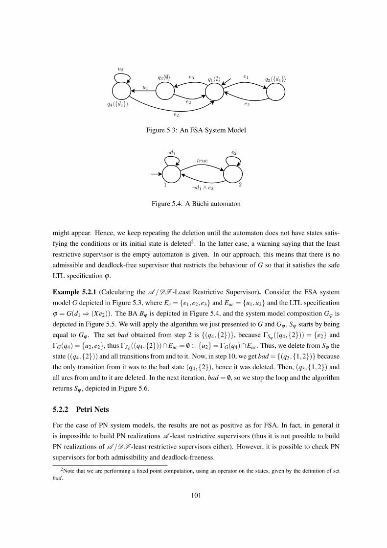
Figure 5.3: An FSA System Model

Figure 5.4: A Buchi automaton

might appear. Hence, we keep repeating the deletion until the automaton does not have states satis-

fying the conditions or its initial state is deleted2. In the latter case, a warning saying that the least

restrictive supervisor is the empty automaton is given. In our approach, this means that there is no

admissible and deadlock-free supervisor that restricts the behaviour of G so that it satisfies the safe

LTL specification ϕ .

Example 5.2.1 (Calculating the A /DF -Least Restrictive Supervisor). Consider the FSA system

model G depicted in Figure 5.3, where Ec = {e1,e2,e3} and Euc = {u1,u2} and the LTL specification

ϕ = G(d1⇒ (Xe2)). The BA Bϕ is depicted in Figure 5.4, and the system model composition Gϕ is

depicted in Figure 5.5. We will apply the algorithm we just presented to G and Gϕ . Sϕ starts by being

equal to Gϕ . The set bad obtained from step 2 is {(q4,{2})}, because ΓSϕ((q4,{2})) = {e2} and

ΓG(q4) = {u2,e2}, thus ΓSϕ((q4,{2}))∩Euc = /0⊂ {u2}= ΓG(q4)∩Euc. Thus, we delete from Sϕ the

state ((q4,{2})) and all transitions from and to it. Now, in step 10, we get bad = {(q3,{1,2})} because

the only transition from it was to the bad state (q4,{2}), hence it was deleted. Then, (q3,{1,2}) and

all arcs from and to it are deleted. In the next iteration, bad = /0, so we stop the loop and the algorithm

returns Sϕ , depicted in Figure 5.6.

5.2.2 Petri Nets

For the case of PN system models, the results are not as positive as for FSA. In fact, in general it

is impossible to build PN realizations A -least restrictive supervisors (thus it is not possible to build

PN realizations of A /DF -least restrictive supervisors either). However, it is possible to check PN

supervisors for both admissibility and deadlock-freeness.

2Note that we are performing a fixed point computation, using an operator on the states, given by the definition of setbad.

101

Figure 5.5: Composition between the FSA system model and the BA

Figure 5.6: The A /DF -least restrictive supervisor obtained after applying Algorithm 4, for Euc ={u1,u2}

Admissibility

We start by briefly describing the negative result of non-existence of PN realizations of A -least re-

strictive supervisors presented in [Giua and DiCesare, 1994a]. To prove the result, a counter-example,

consisting of a PN G to be controlled and a non-admissible supervisor S realized by a PN such that

the A -least restrictive supervisor SA cannot be realized by a PN, is presented. This means that

L Ef in(S

A /G) is a language of finite strings that cannot be generated by a PN, i.e., there is no PN H

such that L Ef in(H/G)=L E

f in(SA /G). This fact is proved using the pumping-lemma for PN languages,

proved in [Jantzen, 1987]. However, when the net is bounded, the A -least restrictive supervisor exists.

In [Giua, 2013] an algorithm for each construction is given. It relies on building the reachability graph

of both the PN model and PN supervisor to find the bad markings, and then using a technique similar

to the construction of minimal satisfying transitions we presented in this work to change the structure

of the PN realization of the supervisor so that it never goes into the set of bad markings. Even though

the final result is a PN built from the original supervisor, this approach requires the construction of the

reachability graph to find the set of bad markings and the transitions that lead to them. Unfortunately,

building the reachability graph is quite computationally expensive. A point to be further studied is

how to build the set of bad markings without building the whole state space.

Given the impossibility of building least restrictive PN realizations of supervisors for the general

case, we now move on to the problem of checking our BA/system model composition for admissibility.

We will briefly address the issue of using control-laws that avoid “forbidden” markings in a least-

restrictive way on top of the BA/system model composition again in the final remarks of this section.

A very recent result [Giua, 2013] provided a procedure for checking admissibility for deterministic PN

102

system models for the case where the specification is a deterministic PN language. However, the result

is obtained under what we prove to be an invalid assumption on the so-called set of uncontrollable

markings. We will point out a counter-example that shows that the set defined there (and in fact used

previously in the literature) as the set of uncontrollable markings is not the set that should be used to

check admissibility. Then, we will define a proper set of uncontrollable markings and show how the

procedure for checking admissibility given in [Giua, 2013] can be adapted. We start by defining the

problem in [Giua, 2013] in our framework.

Problem 5.1. Let G = 〈PG,TG,W−G ,W+G ,MG,0,E, `G〉 and H = 〈PH ,TH ,W−H ,W+

H ,MH,0,E, `H〉 be de-

terministic labelled PNs (G represents the system model and H the PN language specification), where

E = Ec ∪Euc. Let S = 〈PS,TS,W−S ,W+S ,MS,0,E, `S〉 = G ‖ H be the result of the parallel composi-

tion defined in Chapter 2, without the merging of any places3. Decide if S is a PN realization of an

admissible supervisor for G.

The set of events of G and H is the same, thus the language of S is the intersection of the lan-

guages of G and H (all transitions are synchronized). Thus, we have that, taking into account that

the feedback-loop of SC also “implements” the intersection of the languages of the model and the

supervisor:

L (S/G) = L (S)∩L (G) = L (G)∩L (H)∩L (G) = L (H)∩L (G) = L (H/G) (5.15)

Thus, from an implementation point-of-view, using S or H as the supervisor realization is equiv-

alent. However, for analysis, S provides us with extra information: it contains two substructures, one

corresponding to the structure of G and the other corresponding to the structure of H. In particular,

PS = PG∪PH and a marking M ∈ N|PG|+|PH | reachable in S by an event sequence s ∈ E∗ represents the

markings reachable in G and H by executing the same event sequence. Also, the firing of a transition

t = (tG, tH) in S represents the synchronous firing of transition tG in G and transition tH in H. With

this in mind, the notion of uncontrollable marking has been introduced as early as in [Giua, 1992],

as the set of markings M for which an uncontrollable transition t = (tG, tH) in S is not active but for

which tG in G would be active for the projection of M to the places of G:

Mb = {M ∈ N|PG|+|PH | | exists t = (tG, tS) ∈ TS such that tG ∈ Tuc and

for all p ∈ PG, M(p)≥ •t(p) and

exists p ∈ PH such that M(p)< •t(p)}(5.16)

Then, it is proven in Theorem 1 of [Kumar and Holloway, 1996] that S is admissible for G if

and only if none of the markings in Mb is reachable in S. However, this proof does not take into

account the fact that, when building the parallel composition S = G ‖H, one might add more than one

3This means that the places of each PN are considered independent from the places in the other. Using our terminology,in the case of system models with symbolic state description, there are no shared state description symbols and in the caseof system models with algebraic state description, there are no shared places. Note that the notions of parallel compositiondefined for each of these system models coincide in this case.

103

Figure 5.7: (a) A PN generator G, representing the system. (b) A PN generator H, representing thelanguage specification.

Figure 5.8: The parallel composition of G and H of Figure 5.7.

transition for each transition of G. Recall that if T eG is the set of transitions in G labelled with event

e and T eH is the set of transitions in H labelled with the same event e, then the set of transitions in S

labelled with e will be T eG×T e

H . Thus, for each transition tG ∈ T eG, |T e

H | transitions will be created in S.

We illustrate this in the following example.

Example 5.2.2. Consider the deterministic PNs G and H represented in Figure 5.7 (a) and (b) re-

spectively, where event u is uncontrollable, i.e., t1 is an uncontrollable transition. It is clear that both

of them are deterministic. Their parallel composition S = G ‖ H is depicted in Figure 5.8. It is also

clear that S is admissible for G – in fact it does not even restrict the language generated by G. How-

ever, marking[1 0 1

]Tis reachable in S and is clearly in Mb: Transition t = (t1, t2) is such that

M(p1) =•t(p1), where p1 ∈ PG and M(p2)<

•t(p2), where p2 ∈ PH . Thus, Mb, as defined in (5.16),

is not sound, because we need to take into account all transitions in S obtained from t1. This fact is

related to the creation of more than one transition in S corresponding to t1.

This reasoning allows us to formally define the correct notion of uncontrollable marking in S.

Definition 5.2.1 (Uncontrollable Markings). Let G and H be deterministic labelled PNs, S = G ‖ H

104

and Tuc = {t ∈ TG | `G(t) ∈ Euc}. We define the set of uncontrollable markings as:

Muc = {M ∈ N|PG|+|PH | | exists tG ∈ Tuc such that

for all p ∈ PG, M(p)≥ •tG(p) and

for all t = (tG, tH) ∈ TS exists p ∈ PH such that M(p)< •t(p)}(5.17)

A marking M is uncontrollable if exists an uncontrollable transition tG that is active in G by the

projection of M to PG, but all the transitions created from tG in S, i.e. pairs in TG× TH with the

first component equal to tG, are not active in H by the projection of M to PH . Thus, the following

proposition can be proven by a straightforward adaptation for the correct notion of uncontrollable

markings of the proof of Theorem 1 in [Kumar and Holloway, 1996]:

Proposition 5.2.1. Let G and H be two labelled PNs. S = G ‖ H is an admissible supervisor for G if

and only if none of the markings in Muc is reachable in S.

Thus, to solve Problem 5.1, we need to define a procedure to check if an element of Muc is

reachable in S. To do that, we adapt the procedure given in [Giua, 2013], and represent Muc in terms

of partially covering markings for a given marking M.

Definition 5.2.2 (Partially Covering Markings). Let G be a PN system model, M ∈N|P|, and P= ⊆ P.

We define the set of partially covering markings as:

S (M,P=) = {M′ ∈ N|P| |M′(p) = M(p) for all p ∈ P= and M′(p)≥M(p) for all p ∈ P} (5.18)

The set S (M,P=) is the (infinite) set of markings which are equal to M for places in P= and

greater or equal than M for all other places. This set is a generalization of the set defined in [Giua,

2013], where P= is a singleton. However, in spite of being a generalization, checking the reachability

of an element in this set is still decidable4.

Proposition 5.2.2. Let G be a PN system model, M ∈ N|P|, and P= ⊆ P. Checking if a marking in

S (M,P=) is reachable in G, i.e., R(G)∩S (M,P=) 6= /0 is decidable.

Proof. The proof of this proposition relies on a simple adaptation of the construction given in [Giua,

2013].We will reduce the problem of determining if there exists a reachable marking in S (M,P=)

to the problem of determining if a single reachable marking is reachable in a modified net G′ =

〈P′,T ′,W−′ ,W+′ ,M′0〉. he idea of the construction of G′ is to have a PN that initially exactly mimics

the behaviour of G. When G′ gets to a marking M′ that covers M, a special new transition becomes

active. The firing of this transition changes the behaviour of G′ to a behaviour that empties places

in P \ P=, and after all those places have zero tokens G′ enters a deadlocked marking Md . After

this deadlock occurs, if Md(p) = M(p) for all p ∈ P=, then not only was M′ covering M but also

M(p) = M′(p) for all p ∈ P=, i.e., M′ is in S (M,P=) and is reachable in G. Thus, G′ is such that:

4We point out that sets of partially covering markings can have infinite cardinality, and reachability is only proven forfinite sets.

105

• P′ = P∪{ps, p f }

• T ′ = T ∪{t f }∪{tp | p ∈ P\P=}

• W−′is such that:

W−′(p, t) =

W−(p, t) if p ∈ P and t ∈ T

1 if p = ps and t ∈ T

1 if p = ps and t = t f

1 if p = p f and t ∈ {tp | p ∈ P\P=}M(p) if p ∈ P= and t = t f

1 if p ∈ P\P= and t = tp

0 otherwise

(5.19)

• W+′ is such that:

W+′(p, t) =

W+(p, t) if p ∈ P and t ∈ T

1 if p = ps and t ∈ T

1 if p = p f and t = t f

1 if p = p f and t ∈ {tp | p ∈ P\P=}0 if p ∈ P= and t = t f

0 if p ∈ P\P= and t = tp

0 otherwise

(5.20)

• We were redundant in the definition of W−′

and W+′ to facilitate understanding the idea. We

explain in words each of the possibilities:

– W−′

and W+′ coincide with W− and W+ for the original places and transitions in P and

T .

– Place ps is self-looped with all transitions in T .

– The firing of transition t f removes one token from ps and puts it in p f .

– Place p f is self-looped with the transitions in set {tp | p ∈ P\P=}.

– Each place in P\P= is in the preset of t f , with weight M(p).

– Each place p in P\P= is in the preset of the corresponding transition tp.

• M′0 is such that:

M′0(p) =

M0(p) if p ∈ P

1 if p = ps

0 if p = p f

(5.21)

Thus, the evolution of G′ is the following:

106

• Before t f is fired, the evolution is the same as G.

• After t f is fired, all the transitions in t cannot be fired any more, and transitions tp can be fired

until the places p ∈ P \P= become empty. Afterwards, the PN enters a deadlock, where the

number of tokens in places in P= is still the same as it was when t f fired.

• Transition t f only fires when the number of tokens in places p ∈ P\P= is greater or equal than

M(p).

Thus, it is clear that the problem of reaching a marking in S (M,P=) in G is equivalent to the reacha-

bility problem of the (single) marking M′ in G′, where:

M′(p) =

M(p) if p ∈ P=

1 if p = p f

0 if p ∈ P\P′ or p = ps

(5.22)

Before we present the end decidability result, we introduce some helpful notation. We will use

these sets to prove that checking for admissibility is equivalent to checking reachability of a finite

union of sets of partially covering markings.

Definition 5.2.3. Let tG ∈ TG. We define the set of transitions in H that will be synchronized with tGas:

TH(t) = {t ′ ∈ TH | `(tG) = `(t ′)} (5.23)

Definition 5.2.4. Let tG ∈ TG and TH(tG) = {t1, ..., tr}. We define the set of combinations of input

places for the transitions of H that will be synchronized with tG as:

PH(tG) = {p ∈ PH | •t1(p)> 0}×{p ∈ PH | •t2(p)> 0}× ...×{p ∈ PH | •tr(p)> 0} (5.24)

Note that a place p ∈ PH can appear more than one time in a member (p1, ..., pr) of PH(tG) (i.e.,

there can be i, j ∈ {1, ...,r} such that pi = p j = p), in the cases where p is an input place of more than

one transition in TH(tG).

Definition 5.2.5. Let tG ∈ TG, TH(tG) = {t1, ..., tr} and (p1, ..., pr) ∈ PH(tG). We define the set of bad

k’s for tG and (p1, ..., pr) as:

K(tG,(p1, ..., pr)) = {(k1, ...,kr) ∈ Nr | for all i, j = 1, ...,r, ki <•ti(pi) and if pi = p j then ki = k j}

(5.25)

The elements of K(tG,(p1, ..., pr)) will be used to define partially covering markings where

P= = {p1}∪ ...∪{pr}, thus it is necessary to enforce that if pi = p j then ki = k j, so that the par-

tially covering marking is well-defined.

107

Figure 5.9: (a) A PN generator G, representing the system. (b) A PN generator H, representing thelanguage specification.

Example 5.2.3. Figure 5.9 depicts a system model G (a), and a language specification H (b).

Following the definitions above, we have the following:

• TH(t1G) = {t1

H , t3H}

• PH(t1G) = {(p1

H , p3H),(p4

H , p3H)}

• K(t1G,(p1

H , p3H)) = {(0,0),(1,0)}

• K(t1G,(p4

H , p3H)) = {(0,0)}

The set K(tG,(p1, ..., pr)) represents all the possible combinations of tokens in the places p1, ..., pr

that will not make any of the transitions of TH(tG) active. Thus, if tG is uncontrollable, a marking M in

R(S) where (i) M(p)≥ •tG(p) for all p ∈ PG and (ii) there exists (p1, ..., pr) ∈ PH(t) and (k1, ...,kr) ∈K(tG,(p1, ..., pr)) such that M(pi) = ki for all i = 1, ...,r, is an uncontrollable marking. From this

reasoning, we have the following result, adapted from [Giua, 2013]:

Proposition 5.2.3. Problem 5.1 can be reduced to checking reachability of a finite union of sets of

partially covering markings.

Proof. To check admissibility, we need to check if there exists a marking in Muc which is reachable

in S = G ‖ H. To do that, we note that Muc can be represented by a finite union of sets of partially

covering markings. Let tG ∈ Tuc, (p1, ..., pr)∈PH(tG) and (k1, ...,kr)∈K(tG,(p1, ..., pr)), and consider

the marking MtG,(p1,...,pr),(k1,...,kr), defined over PS = PG∪PH as:

MtG,(p1,...,pr),(k1,...,kr)(p) =

ki if p = pi for some element pi of (p1, ..., pr)•tG(p) if p ∈ PG

0 otherwise

(5.26)

108

Note that MtG,(p1,...,pr),(k1,...,kr) is well-defined because (k1, ...,kr) ∈ K(tG,(p1, ..., pr)), and we as-

sume that members of K(tG,(p1, ..., pr)) are such that if pi = p j, then ki = k j, for all i, j ∈ {1, ...,r}.Furthermore, as we previously discussed, the partially covering marking given by

S (MtG,(p1,...,pr),(k1,...,kr),P=), where, given (p1, ..., pr), P= = {p1}∪ ...∪{pr}, represents an infinite

set of markings that are uncontrollable. Also, all the uncontrollable markings can be represented

by partially covering markings, by going through all possible uncontrollable transitions tG ∈ Tuc, all

elements (p1, ..., pr) of PH(tG) and all elements (k1, ...,kr) of K(tG,(p1, ..., pr)). Thus, checking super-

visor admissibility is equivalent to checking that the following finite union of sets of partially covering

markings is not reachable in S:

⋃tG∈Tuc

⋃(p1,...,pr)∈PH(tG)

⋃(k1,...,kr)∈K(tG,(p1,...,pr))

S (MtG,(p1,...,pr),(k1,...,kr),P=) (5.27)

This proposition gives us a procedure to check if a given supervisor S = G ‖ H is admissible:

check reachability in S for all the sets of partially covering markings in the finite union represented in

equation (5.27). If one of them is reachable, then S is not admissible.

We now move on to specialize these result to the composition algorithms we presented. Our

approach, based on the BA/system model composition is a bit different from the traditional approach

based on calculating S = G ‖ H. However, we can frame it so we are in the conditions of applying

Proposition 5.2.3. To do that, we can take Gϕ (i.e., the result of the composition between the system

model G and a BA Bϕ ) and do the following:

1. Rename the places or state description symbols in Gϕ so that there are no shared places or

state description symbols between G and Gϕ . Thus, no place will be merged by the parallel

composition (as defined in this work) of G and Gϕ .

2. Add a place named dead with no preset and initial marking equal to zero, and for each e ∈ Euc

such that there is no transition labelled with e in Gϕ , we add to Gϕ a transition with label e

and only with place dead in its preset (we need this structure because in our case, if e does not

appear in Gϕ it will always be disabled by Gϕ and it is necessary to include this information in

G ‖ Gϕ ).

3. Let G+ϕ the PN obtained after applying the last two steps. Apply Proposition 5.2.3, taking G+

ϕ

as the language specification and S = G ‖ G+ϕ as the candidate supervisor.

The reasoning above also sheds a new light over our approach: we are presenting an LTL-based

approach to build deterministic PN languages specifications. An interesting open question is what is

the class of deterministic PN language specifications that we can specify through syntactically safe

LTL.

109

However, this reasoning for applying Proposition 5.2.3 in our framework requires us to calculate

an extra parallel composition G ‖G+ϕ . In the standard case, a parallel composition between the system

model G and the PN language specification H is needed because the structure of H does not have

any information about the structure of G, and we need that information to check for admissibility.

However, given that Gϕ is obtained by the BA/system model composition, that information is already

present in Gϕ . This means that, we can adapt the result to use Gϕ directly, avoiding the parallel

composition.

The first step of the adaptation is to define the set of uncontrollable markings for Gϕ . Before we

can do it, we define the set of transitions in Gϕ built from a transition t in G.

Definition 5.2.6. G = 〈PG,TG,W+G ,W−G ,MG,0,E, `G,SD〉 be a PN system model (SD is either the sym-

bolic or the algebraic representation, this definition does not depend on it so we keep it general),

tG ∈ TG and Gϕ = 〈PGϕ,T ′Gϕ

,W+Gϕ,W−Gϕ

,MGϕ ,0,E, `′Gϕ,SD〉 be a BA/system model composition. The

set of transitions in Gϕ built from tG is defined as:

TGϕ(tG) = {tGϕ

∈ TGϕ| tGϕ

is of the form ttG,ψ for some BA transition label ψ} (5.28)

The set TGϕ(tG) is simply the set of transitions in Gϕ that were obtained by the creation of the

minimal satisfying transition for tG and a conjunctive clause ψ labelling some transition of the BA.

Definition 5.2.7 (Uncontrollable Marking). Let G = 〈PG,TG,W+G ,W−G ,MG,0,E, `G,SD〉 be a PN sys-

tem model, Gϕ = 〈PGϕ,T ′Gϕ

,W+Gϕ,W−Gϕ

,MGϕ ,0,E, `′Gϕ,SD〉 be a BA/system model composition and

Tuc = {tG ∈ TG | `(tG) ∈ Euc}. We define the set:

Muc = {M ∈ N|PGϕ | | exists tG ∈ Tuc such that

for all p ∈ PG, M(p)≥ •tG(p) and

for all ttG,ψ ∈ TGϕexists p ∈ PGϕ

such that M(p)< •ttG,ψ(p)}(5.29)

The definition is quite similar to the one made for the general case, however, there are two details

that will change the procedure to check if an uncontrollable marking is reachable:

• The BA/system model composition also adds “read-arcs” between the transitions and places in

G. As explained when describing the composition, these arcs are used to restrict the behaviour

of G, avoiding its evolution to markings that do not satisfy any DNF transition labels in the

BA. Thus, transitions ttG,ψ can be disabled even if they are enabled by the substructure of Gϕ

corresponding to the BA.

• The BA/system model composition can outright delete transitions of G, if their firing is guar-

anteed not to satisfy the DNF transition labels of the BA. Thus, it is possible that there is no

transition of the form ttG,ψ in TGϕ, for some transitions tG, i.e., TGϕ

(tG) can be empty.

Thus, taking these 2 facts into account, we adapt Proposition 5.2.3, obtaining Proposition 5.2.4.

110

Figure 5.10: (a) A PN generator G, representing the system. (b) A PN obtained from the BA/systemcomposition, for some BA Bϕ .

Before stating these results, we introduce some helpful notation, adapted from the definitions given

for the standard case.

Definition 5.2.8. Let tG ∈ TG and TGϕ(tG) = {t1, ..., tr}. We define the set of combinations of input

places for the transitions obtained from tG in Gϕ as:

PGϕ(tG) = {p ∈ PGϕ

| •t1(p)− •tG(p)> 0}× ...×{p ∈ PGϕ| •tr(p)− •tG(p)> 0} (5.30)

Note that for Buchi places, i.e., places p ∈ PGϕ\PG, we consider •tG(p) = 0.

Definition 5.2.9. Let tG ∈ TG, TGϕ(tG) = {t1, ..., tr} and (p1, ..., pr) ∈ PGϕ

(tG). We define the set of

bad k’s for tG as:

K(tG,(p1, ..., pr)) = {(k1, ...,kr) ∈ Nr | for all i, j = 1, ...,r,•tG(pi)≤ ki <

•ti(pi) and if pi = p j then ki = k j}(5.31)

Example 5.2.4. Figure 5.10 depicts a system model G (a), and the PN Gϕ resulting from the compo-

sition between G and a BA obtained from some formula ϕ (the formula itself is not important for this

illustration) (b). Note that Gϕ has 2 places b1 and b2 which we assume represent Buchi places.


• TGϕ(t1

G) = {tt1G,ψ1

, tt1G,ψ2}

• PGϕ(t1

G) = {p1G,b1}×{p2

G,b2}= {(p1G, p2

G),(p1G,b2),(b1, p2

G),(b1,b2)}

• K(t1G,(p1

G, p2G)) = {(1,0),(2,0),(1,1),(2,1)}

• K(t1G,(p1

G,b2)) = {(1,0),(2,0)}

• K(t1G,(b1, p2

G)) = {(0,0),(0,1)}

• K(t1G,(b1,b2)) = {(0,0)}

111

With this new definitions, we are in conditions to present a result analogous to Proposition 5.2.3,

adapted to the BA/system model composition.

Proposition 5.2.4. Let G be a PN system model and Gϕ the result of the BA/system model composition

for a syntactically safe LTL formula ϕ . Checking if Gϕ is admissible for G can be reduced to checking

reachability of a finite union of sets of partially covering markings.

Proof. To check admissibility, we need to check if there exists a marking in Muc – defined for the

BA/system model composition – which is reachable in Gϕ . We once again note that Muc can be

represented by a finite union of sets of partially covering markings. Let tG ∈ Tuc, (p1, ..., pr)∈ PGϕ(tG)

and (k1, ...,kr) ∈ K(tG,(p1, ..., pr)), and consider the markings MtG,(p1,...,pr),(k1,...,kr) and MtG , defined

over PGϕas:

MtG,(p1,...,pr),(k1,...,kr)(p) =

ki if p = pi for some element pi of (p1, ..., pr)•tG(p) if •tG(p)> 0

0 otherwise

(5.32)

MtG(p) =

{•tG(p) if p ∈ PG

0 otherwise(5.33)

MtG,(p1,...,pr),(k1,...,kr) is defined analogously to the previous definition – the only difference is on

how one defines the parameters (p1, ..., pr) and (k1, ...,kr). In this case, we also define marking MtG ,

that will be used for the case of transitions tG ∈ TG for which no transition of the form ttG,ψ were

created in Gϕ . These markings are used to reduce the coverability problem for markings for which tGwould be active to the reachability problem of partially covering markings. Thus, given (p1, ..., pr), let

P= = {p1}∪ ...∪{pr}. Checking supervisor admissibility is equivalent to checking that the following

finite union of sets of partially covering markings is not reachable in Gϕ :

⋃tG∈Tuc | TGϕ (tG)6= /0

⋃(p1,...,pr)∈PGϕ (tG)

⋃(k1,...,kr)∈K(tG,(p1,...,pr))

S (MtG,(p1,...,pr),(k1,...,kr),P=)

⋃⋃tG∈Tuc | TGϕ (tG)= /0

S (MtG , /0)

(5.34)

This approach for checking admissibility can be easily adapted to calculate the set of reachable

uncontrollable markings itself, thus it can also provide a finite representation of all the reachable

markings in the supervisor that will disable uncontrollable events that are active in G. Thus, if we can

also calculate the deadlocked markings in the same way, we will have a finite representation of the set

equivalent to set bad defined for FSA, i.e., the set of all the markings in Gϕ that should be avoided in

order to guarantee admissibility.

112

Deadlock-Freeness

Continuing from the discussion above, we will show that in fact, the deadlocked markings can also be

represented by sets of partially covering markings. We start by defining the set of deadlocked markings

for an arbitrary PN structure N. Given that, in the case of the BA/system model composition, the active

events in Gϕ are always a subset of the active events in G, it will be enough for our case to check Gϕ

for deadlocked markings.

Definition 5.2.10 (Deadlocked Marking). Let N = 〈P,T,W−,W+,M0〉 be a PN structure. The set of

deadlocked markings for N is defined as:

Mdead = {M ∈ N|P| | for all t ∈ T exists p ∈ P such that M(p)< •t(p)} (5.35)

It is clear from the definition that if a marking in Mdead is reachable in N, then N is not deadlock-

free. Before we provide the reduction from checking for deadlock-freeness to reachability of a finite

union of sets of partially covering markings, we, again, present some useful notation. This definitions

are analogous to the ones presented for admissibility, but taking into account that for the case of

deadlock-freeness we are interested in representing markings for which none of the transitions is

active.

Definition 5.2.11. Let N = 〈P,T,W−,W+,M0〉 be a PN structure, where T = {t1, ..., tm}. The set of

tuples of places associated to a deadlock marking in N is given by:

Pdead = {p ∈ P | •t1(p)> 0}×{p ∈ P | •t2(p)> 0}× ...×{p ∈ P | •tm(p)> 0} (5.36)

For each tuple of places in Pdead , we also define the set of bad k’s.

Definition 5.2.12. Let N = 〈P,T,W−,W+,M0〉 be a PN structure, where T = {t1, ..., tm}, and

(p1, ..., pm) ∈ Pdead . The set of bad k’s for (p1, ..., pm) is given by:

K((p1, ..., pm)) = {(k1, ...,km) ∈ Nm | for all i, j = 1, ...,m, ki <•ti(pi) and if pi = p j then ki = k j}

(5.37)

Example 5.2.5. Figure 5.11 depicts a PN structure N.


• Pdead = {p1, p2}×{p2, p3}= {(p1, p2),(p1, p3),(p2, p2),(p2, p3)}

• K((p1, p2)) = {(0,0),(1,0),(0,1),(1,1)}

• K((p1, p3)) = {(0,0),(1,0)}

• K((p2, p2)) = {(0,0)}

• K((p2, p3)) = {(0,0),(0,1)}

113

Figure 5.11: A PN structure N.

Note that for K((p2, p2)) we did not add (0,1) because that would require for M(p2) to have two

different values at the same time.

We are now in conditions to state the main result of this subsection.

Proposition 5.2.5. Let N = 〈P,T,W−,W+,M0〉 be a PN structure, where T = {t1, ..., tm}. Checking

if N is deadlock-free can be reduced to checking reachability of a finite union of sets of partially

covering markings.

Proof. To check deadlock-freeness, we need to check if there exists a marking in Mdead . Let

(p1, ..., pm) ∈ Pdead and (k1, ...,km) ∈ K((p1, ..., pm)), and consider the markings M(p1,...,pm),(k1,...,km)

defined over P as:

M(p1,...,pm),(k1,...,km)(p) =

{ki if p = pi for some element pi of (p1, ..., pm)

0 otherwise(5.38)

Note that M(p1,...,pm),(k1,...,km) is well-defined because (k1, ...,km) ∈ K(t,(p1, ..., pm)), and we as-

sume that members of K(t,(p1, ..., pm)) are such that if pi = p j, then ki = k j. Furthermore, it is

easy to see that the partially covering markings given by S (M(p1,...,pm),(k1,...,km),P=), where, given

(p1, ..., pm), P= = {p1}∪ ...∪{pm}, represent an infinite set of deadlocked markings. Also, all the

deadlocked markings can be represented by partially covering markings, by going through all ele-

ments (p1, ..., pm) of Pdead and all elements (k1, ...,km) of K((p1, ..., pm)). Thus, checking supervisor

deadlock-freeness is equivalent to checking that the following finite union of sets of partially covering

markings is not reachable:

⋃(p1,...,pm)∈Pdead

⋃(k1,...,km)∈K((p1,...,pm))

S (M(p1,...,pm),(k1,...,km),P=) (5.39)

There are many other approaches for deadlock-freeness checking, we presented this one to keep

ourselves consistent with what we presented for admissibility checking and also to provide motivation

114

for further work. It is known that checking deadlock-freeness is an EXPSPACE-hard problem for

arbitrary PNs [Cheng et al., 1993], thus we cannot expect to solve it efficiently for bigger systems.

There are many approaches for checking deadlock freeness, we refer the reader to [Girault and Valk,

2002] which covers an array of state-of-the-art analysis techniques for this problem.

The enforcement of deadlock-freeness in PN models through SC is still a big challenge for the PN

community and there are many different approaches for solving the problem, though the main bulk

of them does not deal with uncontrollable events. In general, there is a trade-off between the non-

restrictiveness of a supervisor and the amount of computational effort that is needed to calculate it, and

there are several surveys exclusively dedicated on comparing the wide array of different approaches

(some of them for specific classes of PNs). We refer the reader to, for example, [Li et al., 2012, Li

et al., 2008, Li and Zhou, 2009] to surveys on this subject. Most of these approaches do not deal with

uncontrollable events, thus we highlight [Iordache et al., 2002] which takes this notion into account.

5.3 Specification Language Restriction for Admissibility

As mentioned in the previous section, given the limitations of modular SC theory and the SC of PNs,

we present a restriction to the syntactically safe LTL formulas that guarantees supervisor admissibility.

We will present the restriction for all system models.

We start by defining the set of controllable literals which is composed of literals for which the

truth value is not changed by the occurrence of uncontrollable events. This means that our supervisor

can always enforce that an element of Dc must be satisfied, while being admissible.

Definition 5.3.1 (Controllable State Description Literals – FSA System Models). Let

G = 〈Q,E,δ ,q0,D,µ〉 be an FSA system model. The set litc of controllable state description literals

is defined as:

litc = {l ∈ lit(D) | For all q ∈ Q and e ∈ Euc∩ΓG(q), if µ(q) l then µ(δ (q,e)) l} (5.40)

To check is a given state description literal l is controllable, we need to analyse all states where l

is satisfied. If for all of these states there is no uncontrollable event that can occur and drive the FSA

to a state where l is not satisfied, then l is controllable.

Example 5.3.1 (Controllable State Description Literals – FSA). Consider the FSA system model in

Figure 5.12. In order to simplify the example, δ is only defined for state x, but in general one needs

to do this analysis for all states that satisfy a given literal. We assume that event e is controllable

and event u is uncontrollable. It is possible to see that literal d2 is not controllable: µ(x) d2 but

µ(z) 6 d2 and δ (x,u) = z. On the other hand, literal ¬d3 is controllable: µ(x) ¬d3, µ(z) ¬d3 and,

in spite of µ(y) 6 ¬d3, the event that drives x to y is controllable, thus can be disabled. With a similar

reasoning, we can check that literal d1 is also controllable. All the other literals, i.e., ¬d1, ¬d2 and d3

are not satisfied in x, hence are also controllable.

115

Figure 5.12: Checking which state description literals are controllable – FSA.

Figure 5.13: Checking which state description literals are controllable – PN with symbolic state de-scription.

Definition 5.3.2 (Controllable State Description Literals - PN with Symbolic State Description). Let

G = 〈P,T,W+,W−,M0,E, `,D,µ〉 be a PN system model. The set litc of controllable state description

literals is defined as:

litc = {l ∈ lit(D) | for all t ∈ Tuc, if •t(µ(l)) = 1 then t•(µ(l)) = 1}

The set litc contains the literals associated to places that are not in the preset of an uncontrollable

transition or, if so, are also in the postset of that transition. This means that our supervisor can always

enforce that the truth value of elements l of litc cannot be altered while being controllable, because

we can disable all transitions that can change the marking of the place corresponding to l, µ(l), since

such transitions correspond to controllable events.

Example 5.3.2 (Controllable State Description Literals - PN with Symbolic State Description). In

Figure 5.13, we show an example of a PN system model, where event e is controllable and event u

is uncontrollable. The set of uncontrollable transitions is Tuc = {t2}. The state description literal d1

is controllable because •t2(p1) = 0, and ¬d1 is uncontrollable because •t2(p2) = 1 (i.e., p2 is in the

preset of t2) and t•2(p2) = 0 (i.e., p2 is not in the postset of t2).

Definition 5.3.3 (Controllable State Description Literals - PN with Algebraic State Description). Let

G = 〈P,T,W,M0,E, `,κ, 〉 be a PN system model. The set litc of controllable state description literals

is defined as:

litc = {(p,b) ∈ Pb×N | for all t ∈ Tuc, if t•(p)− •t(p)< 0 then t•(p)≥ b}

The set litc corresponds to pairs of places and positive integers p,b for which, if the firing of

an uncontrollable transition consumes tokens from it, then that firing puts in the place an amount of

tokens greater or equal than b.

116

Figure 5.14: Checking which state description literals are controllable – PN with algebraic state de-scription.

Figure 5.15: BA that generates the language satisfying type 1 formulas.

Example 5.3.3 (Controllable State Description Literals - PN with Algebraic State Description). In

Figure 5.14, we show an example of a PN system model, where event e is controllable and event u is

uncontrollable. The set of uncontrollable transitions is Tuc = {t1}. Literals M(p1 ≥ 1) and M(p1 ≥ 2)

are controllable, because though t•1(p1)− •t1(p1) =−1 < 0, t•1(p1) = 2.This means that immediately

firing t1, p1 will have at least 2 tokens. Also, for all b ≥ 3, M(p1) > b is an uncontrollable literal.

Since no uncontrollable transition takes tokens from p2, the literals M(p2)≥ b are controllable for all

b ∈ N.

Definition 5.3.4 (LTL Formula Restrictions for Supervisor Admissibility). LTL specifications ϕ must

be of one of the following types:

Type 1. Gψ , where ψ is a propositional formula in the DNF where only literals in litc that are satisfied

in the initial state, or literals ¬e with e ∈ Ec can occur. This type of formula can be encoded as

the deterministic BA in Figure 5.15.

Type 2. G(γ⇒ Xψ), where γ is any propositional formula in the DNF and ψ is a propositional formula

in the DNF where only literals in litc that also appear in γ , or literals ¬e with e ∈ Ec can occur.

This type of formula can be encoded as the deterministic BA in Figure 5.16.

Type 3. G(γ⇒ X(ψWγ ′)), where γ and γ ′ are any propositional formulas in the DNF and ψ is a propo-

sitional formula in the DNF where only literals in litc that also appear in γ , or literals ¬e with


117


e ∈ Ec can occur. This type of formula can be encoded as the deterministic BA in Figure 5.17.

The BA were obtained by determinizing the BA obtained from LTL2BA [Gastin and Oddoux,

2001], but if one carefully analyses them, it is clear that they accept exactly the ω-strings that satisfy

the formulas.

Formulas of type 1 are formulas that specify propositional logic relations between state descrip-

tions and controllable events that should always be satisfied in all markings of the supervised PN. For

example, we might want that two given robots do not move at the same time or that a certain control-

lable event never occurs. To ensure admissibility, we only allow the occurrence in ψ of literals in litcor the negation of controllable events.

Formulas of type 2 specify that the propositional logic formula ψ must be satisfied exactly after

condition γ is met. For example, we may specify that if a robot is moving forward and there is no

obstacle in front of it, it should continue moving forward:

G((moving f orward∧no obstacle)⇒ (Xcontinue moving)) (5.41)

Since γ is a condition, it can have occurrences of all atomic propositions. To ensure admissibility,

we require that only literals in litc that also appear in γ or the negation of controllable events can

occur in ψ . This means that, in this type of formula, one can require that a given controllable state

description symbol maintains its truth value but cannot enforce the occurrence of an event that changes

it.

Formulas of type 3 specify that immediately after condition γ is satisfied, the propositional formula

ψ must keep being satisfied until condition γ ′ is met. For example, if a robot is moving forward and

there is no obstacle in front of him, it should continue moving forward until the goal region is reached.

G((moving f orward∧no obstacle)⇒ (X(continue movingWgoal reached))) (5.42)

The restrictions for the literals appearing in ψ are the same as for formulas of type 2. We also note

that, using this kind of formula, one can state that, after condition γ is met, a given controllable event

should be the next controllable event to occur. This can be seen as stating that a given controllable

event should occurs as soon as possible. Let e ∈ Ec be that event. The following formula of type 3 is

118

a translation to LTL of the previous natural language statement:

G(γ ⇒ X((∧

e′∈Ec\{e}¬e′)We)) (5.43)

These 3 types of formulas already allow us to specify a wide array of different behaviours for

a system to fulfil. In fact, in our experience, all the natural language specifications we defined for

several different examples can be translated into LTL formulas of one of these types. We note that an

LTL formula of one of these types ensures admissibility of the supervisor because:

• We never enforce that a token must remain in a place that is in the preset of an uncontrollable

transition;

• We never enforce that a token must not be put in a place that is in the postset of an uncontrollable

transition;

• We never enforce the occurrence of an event or set of events, we may only enforce that a given

subset of Ec must not happen at a given moment.

We now prove this statement using the BA obtained for each type of formula.

Proposition 5.3.1. Let G be a PN system model and ϕ a formula of type 1, 2 or 3. Then Gϕ is

admissible for G.

Proof. We first start by analysing what are the labels that cannot be satisfied in each state of the BA

for each type of formula.

• For type 1 formulas, it is clear that any transition firing that satisfies ¬ψ will be disabled when

the BA is in state x.

• For type 2 formulas, if the BA is in state x, then any transition firing that does not satisfy none

of the DNF labels of arcs from state x, i.e., when it satisfies ¬(¬γ ∨ γ) = γ ∧¬γ = f alse. Thus,

when the BA is in state x, all transitions can fire. When the BA is in state y, transitions that do

not satisfy either ψ ∧ γ or ψ ∧¬γ are disabled, that is, the transitions that will be disabled will

be the ones for which the firing satisfies:

¬((ψ ∧ γ)∨ (ψ ∧¬γ)) = ¬(ψ ∧ γ)∧¬(ψ ∧¬γ)

= (¬ψ ∨¬γ)∧ (¬ψ ∨ γ)

= (¬ψ ∧ (¬ψ ∨ γ))∨ (¬γ ∧ (¬ψ ∨ γ))

= (¬ψ ∧¬ψ)∨ (¬ψ ∧ γ)∨ (¬γ ∧¬ψ)∨ (¬γ ∧ γ)

= ¬ψ ∨ (¬ψ ∧ γ)∨ (¬ψ ∧¬γ)

= ¬ψ

Thus, any transition firing that satisfies ¬ψ will be disabled when the BA is in state y.

119

• For type 3 formulas, the reasoning for state x is analogous to the reasoning for type 2 formulas,

and we can conclude that no transition will be disabled. When the BA is in state y, transitions

that do not satisfy either ¬γ ∧ γ ′ or (ψ ∧ γ)∨ (ψ ∧¬γ ′)∨ (γ ∧ γ ′) are disabled. With the same

type of calculation as above, we get that transitions for which the firing satisfies (¬γ ′∧¬ψ) are

disabled. Thus, the set of transitions which are disabled in state y is a subset of the transitions

for which the firing satisfies ¬ψ .

From the reasoning above, we can conclude that it is sufficient to show that the firing of an uncon-

trollable transition will never satisfy (¬ψ). This is a direct consequence of the restrictions we put on

ψ:

• Given that we can only write negations of controllable events in ψ , ¬ψ the only elements of

lit(E) in ¬ψ will be positive literals e ∈ Ec. The label of an uncontrollable transition is in Euc,

hence it will never satisfy any of the event literals.

• We can only write controllable literals in ψ , where, for formulas of type 1, those literals are

satisfied in the initial marking and, for formulas of type 2 and 3, those literals also appear in

γ . Furthermore, for formulas of type 2 and 3, γ needs to be satisfied to make the BA go to

state y. Thus, a firing of a transition satisfies ¬ψ when it changes the PN from a marking M

that satisfies all the controllable literals in ψ to a marking M′ for which at least one of the

controllable literals in ψ is not satisfied. Given our definition of controllable literal, it is clear

that none of the uncontrolled transitions will have this behaviour, hence, no uncontrollable

transition satisfies ¬ψ , i.e., no uncontrollable transition is disabled.

5.4 Decentralized Approach

In the particular case of multi-robot systems, a drawback of the presented methodology is related to its

centralized nature, which induces high complexity and low tolerance to failures during execution. To

mitigate this problem, we present a first approach for a decentralized version, where each robot runs an

individual PN controller and an individual set of PN realizations of supervisors. This approach is based

on the individual robot PN system models with symbolic state description and the LTL specifications

for each individual robot. It relies on augmenting the individual PN system models and creating a

communication scheme. Robots communicate both changes in the environment and occurrence of

events that are relevant for the coordination (the relevant data to be communicated is obtained from

the LTL specifications), and the PN models of each robot are augmented so that the markings can be

updated by the occurrence of these communication events. Thus, one can avoid building the parallel

composition of the individual models to obtain a model of the multi-robot team, while still being

able to use the BA/system model composition presented in the previous chapter for each individual

120

PN model and each LTL specification. One can then deploy, for each robot, the corresponding PN

supervisors. The work presented in this section was first described in [Lacerda and Lima, 2011c].

In the following, we assume a team of n robots, with individual PN system models with symbolic5

state description Gi =⟨Pi,Ti,W−i ,W+

i ,M0i,Di,µi⟩, i = 1, ...,n. Each robot model event set is parti-

tioned into controllable and uncontrollable events, i.e., Ei = Ec,i ∪Euc,i. The set E of events of the

system is the union of the events of each individual model and the set D of state description symbols

of the system is the unions of the state description symbols for each individual model.

We start by defining the sets of shared events and shared state description symbols, for each robot

i.

Definition 5.4.1 (Shared Events). The set of shared events for robot i is defined as:

Esi =

n⋃j=1j 6=i

Ei∩E j (5.44)

Shared events represent the triggering of collaborative actions between the robots.

Definition 5.4.2 (Shared State Description Symbols). The set of shared state description symbols for

robot i is defined as:

Dsi =

n⋃j=1j 6=i

Di∩D j (5.45)

Shared state description symbols represent environmental changes that are present in the model of

more that one robot and/or can happen due to more than one robot. In this case, we need to add a new

restriction to the set of controllable state description literals used to restrict the specification language.

Due to the decentralized nature of this solution, each robot cannot guarantee that its teammates will

not alter the truth value of its shared description symbols. Hence, we also exclude it from the set of

controllable state description literals.

Definition 5.4.3 (Controllable State Description Literals). The set litc,i of controllable state descrip-

tion literals for robot i is defined as:

litc,i = {l ∈ lit(Di) | l 6∈ lit(Dsi ) and for all t ∈ Ti,uc,

•t(µi(l)) = 0} (5.46)

Remark 5.4.1. To guarantee that a shared state description symbol d remains unaltered, we need to

check if all the robots that share d have similar LTL specifications regarding it. This would imply

analysing the LTL specifications for all the robots sharing d, which is subject of future work.

We will write n sets of specifications, one for each robot.6 For robot i, the formulas are written

over Π = E ∪D, i.e., over the events and state description symbols of the whole system. We comply5This approach was developed only for this type of system model.6A subject of future research is following the more elegant approach of writing global specifications – that can include

shared description symbols in the set of controllable literals for the team – to be satisfied in a local and decentralized way.

121

with the admissibility rules but, for each robot i, we take into account the sets Ec,i and litc,i instead

of the sets Ec and litc taken into account in the centralized version. This is because we are building

local supervisors for each robot, and we cannot have a supervisor for robot i disabling actions that

are related to robot j (but a supervisor of robot i might change the behaviour of i after j executes an

action, for example). Hence the writing of specifications over E ∪D.

Formally, we are interested in solving the following problem:

Problem 5.2. Given n individual PN models G1, ...Gn and sets Φ1, ...Φn, where Φi = {ϕ1i , ...,ϕ

mii }

is the set of LTL specifications for each robot, written over the set Π = E ∪D, and satisfying

Definition 5.3.4 (using the sets Ec,i and litc,i instead of Ec and litc) build, for each robot i:

• An augmented model Gcommi that handles the required communications between robot i and

other robots;

• mi admissible PN realizations of supervisors Sϕ1

i, ...,S

ϕmii

such that L D(Gcommi /S

ϕ1i, ...S

ϕmi1) is the largest language contained in L D(Gcomm

i ) such that:

If σ ∈L D(Gcommi /S

ϕ1i, ...,S

ϕmii) then σ ϕ

ji for all j = 1, ...,mi (5.47)

To solve this problem, we will define the augmentation of each individual PN model, which is

based in the sets of shared events and shared state description symbols and in the LTL specifications.

Afterwards, we compose the augmented PNs with the BA obtained from the formulas, following

Algorithm 3.

We describe the process for a given robot i. The approach is analogous for all other members of

the team. For each robot i, we start by defining the sets of robots that share events e ∈ Esi and state

description symbols d ∈ Dsi with i, i.e., robots that need to communicate with i to execute e or to

inform i that the truth value of d has changed.

Definition 5.4.4 (Robots Sharing an Event with i). Let e ∈ Esi . The set of robots sharing an event with

i is defined as:

commie = { j ∈ {1, ...,n} | j 6= i and e ∈ Ei∩E j} (5.48)

The set of shared events with robot i represents the triggering of collaborative actions between the

robots for which robot i must be involved, e.g., in a robot soccer scenario, a pass from another robot

to robot i. To fire transitions associated to shared events, the robots must communicate and make sure

that all the involved robots are ready to execute the action. Since all the models already include these

shared actions, there is no need of adding anything to the individual PNs.

Definition 5.4.5 (Robots Sharing a State Description Symbol with i). Let d ∈ Esi . The set of robots

sharing a state description symbol with i is defined as:

commid = { j ∈ {1, ...,n} | j 6= i and d ∈ Di∩D j} (5.49)

122

Figure 5.18: (a) A PN system model for an individual robot. (b) The individual model after addingthe transitions to handle communication, for shared state description symbol d2.

The set of shared state description symbols for robot i represents environmental changes that can

happen or be observed by robot i and also by other robots. Whenever the truth value of a shared

state description symbol d is changed by a team member, i.e., whenever one of the robots j ∈ commid

goes from a marking M to a marking M′ such that M(µ(d)) 6= M′(µ(d)) (equivalently, M(µ(¬d)) 6=M′(µ(¬d))), it needs to send a message to robot i saying that d has changed and what is its truth

value. The individual PN model of robot i needs to be augmented to handle this change in d in the

cases where it did not observe it. To do this, we add two new uncontrollable events to Ei, named

change d true and change d f alse. We also add 4 transitions to Ti to cover the following cases:

1. Message from j ∈ commd stating that the truth value of d changed to true, and it is already true

in the current marking of i.;

2. Message from j ∈ commd stating that the truth value of d changed to true, and it is f alse in the

current marking of i;

3. Message from j ∈ commd stating that the truth value of d changed to f alse, and it is already

f alse in the current marking of i;

4. Message from j ∈ commd stating that the truth value of d changed to f alse, and it is true in the

current marking of i;

The first two cases deal with the situations where when the robot receives the message, it already

observed the change of the truth value of d. The last two cases deal with the situations where the

message states a change of the truth value of d that the robot did not observe. In Figure 5.18 (a) we

depict an individual PN system model, and in Figure 5.18 (b), we depict the model after adding the

transitions for a shared state description symbol d2.

123

We also need to take into account the information needed to fulfil the LTL specifications, which,

as stated before, are written over the set Π = E ∪D. We start by defining the sets of occurrences of

events and state description symbols for a given formula ϕ .

Definition 5.4.6 (Occurrences of Symbols in ϕ). Let ϕ be an LTL formula for robot i, written over

E ∪D. The sets of events and state description symbols occurring in ϕ are defined as:

occEϕ = {e ∈ E | e occurs in ϕ} (5.50)

occDϕ = {d ∈ D | d occurs in ϕ} (5.51)

These sets contain, respectively, the elements of E that occur in ϕ and the elements of D that occur

in ϕ . We will need to augment Gi so that it can handle the events and state description symbols that

occur in ϕ but are not in Gi. Hence, we define the sets of external events and external state description

symbols in extEϕ and extD

ϕ .

Definition 5.4.7 (External Symbols in ϕ). Let ϕ be an LTL formula for robot i, written over E ∪D.

The sets of external events and external state description symbols of ϕ are defined as:

extEϕ = occE

ϕ \Ei (5.52)

extDϕ = occD

ϕ \Di (5.53)

External events and external state description symbols represent information about the global state

of the system that is needed for robot i to satisfy ϕ , but that are not included in the individual PN model

for robot i. The elements d of extDϕ are handled in a similar manner as the shared state description

symbols. The difference is that we also need to add d to Di and add two places to Pi corresponding

to µ(d) and µ(¬d) and do not need to add transitions that represent that the robot already observed a

change on the truth value of d before receiving the communication, as depicted in Figure 5.19. The

initial marking of these places can be obtained from the initial marking of a PN G j such that d ∈D j7.

Also, we add i as a communication target for the change of the truth value of d in the PNs G j such

that d ∈ D j.

For the elements of extEϕ , we simply add e to Ei as an uncontrollable event and a transition t with

label e that is always active to Ti and fires without changing the marking of Gi. For example, Figure

5.20 depicts the place and transitions added to Gi if extEϕ = {e4,e5,e7}. Furthermore, whenever a

robot j such that e ∈ E j fires a transition with label e, it sends a message to i which also fires its added

transition with label e – this maintains Gi in the same marking, but will change the marking of the

supervisor obtained from ϕ , thus changing the set of enabled events.

Following this procedure for each robot i, we obtain the augmented PN models Gcommi to be

composed with the BA. Note that in these augmented models we added exactly the external events

7We continue assuming that the initial markings are consistent.

124

Figure 5.19: (a) A PN system model for an individual robot. (b) The individual model after addingthe places and transitions to handle communication, for external state description symbol d3.

Figure 5.20: (a) A PN system model for an individual robot. (b) The individual model after addingthe place and transitions to handle communication, for external events {e4,e5,e7}.

125

and state description symbols that are required to evaluate the LTL specifications. In the centralized

case, where we model multi-robot systems by using parallel composition, the model to be composed

with the BA is larger, since it takes into account all events and state description symbols of all robots.

We will see in the next Chapter that the decentralized approach is a relevant improvement in terms

of supervisor size executed for each robot, not only because only relevant external events and state

description symbols are added to the individual models but also because they can be executed in a

decentralized manner, thus each robot executes the same number of modular supervisors regardless of

the number of robots in the team.

This procedure is yet to be tested in a real scenario and can still be subject to a number of improve-

ments. An obvious improvement is abstracting, when possible, which robot sent the communication.

This would be done by having external events that can be fired whenever there is an incoming com-

munication of the occurrence of an event for which the receiving robot does not need to know the id

of the robot that executed it to fulfil the specification. By doing this, we would be able to add and

subtract elements to the team without the need to change the models and the specifications. Also, this

approach can be generalized for PN models with algebraic state description.

5.5 Generalized Mutual Exclusion Constraints

We finish the chapter with a brief remark on an alternative approach for SC of PNs. The first is

from a theoretical point-of-view. The most studied and used approach for SC using PN is arguably

the so called generalized mutual exclusion constraints (GMEC) approach. There has been many

works on the use of this approach, as was mentioned in the section about related work, e.g., [Giua

et al., 1992, Iordache and Antsaklis, 2006b,Wu et al., 2002, Iordache and Antsaklis, 2002,Moody and

Antsaklis, 1998, Iordache and Antsaklis, 2006a]. The problems we addressed in this section have all

been studied for GMECs, and there are methods to build (non least-restrictive) supervisors that ensure

admissibility and deadlock freeness. They also address other issues such as unobservable events and

liveness, though for some of these cases – particularly the ones related to deadlock prevention and

liveness enforcement – the approach can be quite inefficient, in the sense that its complexity is quite

high and solutions can only be found for more or less small cases. Contrary to our approach, the

GMEC approach is not based on language specifications. It is based on the addition of places –

called monitors – that create place invariants in the PN. These monitors allow the designer to write

specifications similar to our specifications for the algebraic state description (in the basic form, without

taking events into account). In fact, the construction of the counter place we presented here has

similarities with the basic construction of monitors. The main differences between the approaches

is that, while our approach allows the use of LTL specifications written over linear combinations

of the number of tokens in bounded places, the GMEC approach allows writing specifications over

linear combinations of the number of tokens in places that must be satisfied in all the markings of

the PN. Loosely speaking, a “GMEC specification” lT M ≥ b is equivalent to G(lT M ≥ b) in our

126

case (assuming that the specifications are only over bounded places). The GMEC approach has the

advantage of being able to deal with unbounded places. However, this is the case because, since the

idea of GMEC is to always keep the number of tokens in the places above or below a given constant,

being only applicable when the initial marking already satisfies the linear constraint, there is no need

to “check” the number of tokens in the places being controlled. In our case that kind of checking

is necessary, because we always need to check what is the marking after the firing of a transition in

order to make the BA evolve to the correct state. Thus, since it is known that any extension of the

PN model that allows checking an unbounded place for 0 tokens increases the modelling power of the

extended PN model to the power of Turing machines (which is not desired, since for Turing machines

most non-trivial problems are undecidable), we cannot hope to extend our approach to reason directly

about unbounded places (however, we note that unbounded places can be present in the PN, we are

just not able to refer to them in the LTL formulas). Even if there is the possibility to deal with

unbounded places in some cases – for example the specification G(lT M ≥ b) has the same flavour as a

GMEC specification, thus for this case it is possible to build a supervisor – most of the LTL formulas

will require some checking on the number of markings in the places it refers to. The approach has

also been extended in order to also take into account linear constraints on the firings of transitions.

Furthermore, there has been a small reference on how this approach can be used to find admissible

supervisors for PN language specifications, but, to the best of our knowledge, the amount of research

on this topic is limited to just one small section in [Iordache and Antsaklis, 2006b]. Furthermore, it

would require the calculation of G ‖Gϕ , which is something that we want to avoid. We argue that, the

algorithm we presented to directly verify Gϕ for admissibility is a better approach in our case.

127

CHAPTER 6

Case Studies and Results

In this chapter, we present three application scenarios of the methodologies we presented. We will

start with a simulated soccer robot team. This is a simple example where the individual models are

not very intricate. It is presented with the goal of providing a simple illustration of the methodology

and comparing the different approaches we developed in terms of scalability. We will then present

implementations on a social robot and on a multi-robot surveillance scenario, which illustrate the

application of our methodology to real robot systems. Before describing the scenarios themselves, we

present some practical remarks about their implementation.

As we discussed in Section 5.2, there is still considerable work to be done in order to efficiently

obtain admissible and deadlock-free PN supervisors. This is a point for future work, however, in order

to be able to implement our methodology in concrete scenarios, we took a more pragmatic point-of-

view. Given that the state-of-the-art still does not allow one to build admissible and deadlock-free

supervisors for complex systems, in order to implement our work in real systems, our approach will

be the following:

• In Sections 6.1 and 6.3, will use the extra restriction to the syntactically safe LTL specifications

– presented in Section 5.3 – that guarantees supervisor admissibility by construction. It has

the drawback of mixing the specification and model levels, which is not always desired. For

example, when the writing of the specifications depends directly on the model, any change in it

can have a large impact on the specification. However, when the designer feels it is appropriate –

for the case of our application scenarios for example, we had no problems using the restriction

– the admissibility restriction provides a guarantee that, as we have just discussed, is very

computationally expensive to check for complex systems.

• In Section 6.2, the admissibility restriction for the specifications is not used, because at the time

129

the example was implemented we had not defined the language restriction. In this case, we add

an extra rule to the evolution of the supervisor: always enable all uncontrollable events and if

the system executes one which is not active in the current state of the supervisor, simply ignore

it (i.e., the supervisor does not execute an event). Of course, this might lead to unpredictable be-

haviours. However, in this particular example, the impact of ignoring non-active uncontrollable

events on the final behaviour of the system was not noticeable.

• For deadlock-freeness, one can either try and apply a deadlock freeness algorithm or, as was

our choice, proceed with simulations before deployment and check if blocking occurs. If so,

the specifications should be rewritten. This is obviously a very naive approach, which does not

provide guarantees, but in our cases we managed to get supervisors which never deadlocked,

after a small amount of simulation-specification rewrite iterations.

In the application scenarios where we used the language restriction to guarantee admissibility, we

could translate our natural language specification to formulas of type 1, 2 or 3 in a intuitive way, so

we argue that the restriction already allows the definition of a good array of behaviours. However, our

ultimate goal is to continue developing the methodology so that we can eventually drop the use of this

language restriction.

In terms of execution, whenever there are active controllable events, we immediately choose one

randomly to be executed. When there are only uncontrollable events, we wait until one of them

becomes active and, when it does, we fire it accordingly, update the system and supervisors states and

check for active controllable events to fire next.

To finalize this overview of the practical implementation of our methodology, we just mention an-

other approach that can be used when dealing with homogeneous multi-robot teams: do the analysis

for a small amount of robots (e.g., 3 robots) and, if needed, modify the specifications to guarantee

supervisor admissibility and deadlock-freeness. Then, since the addition of more robots only en-

tails the addition of another module similar to the ones already in the model, and a small change

in the specifications, it might be possible to guarantee that if we have supervisory admissibility and

deadlock-freeness for a given set of specifications, the adding of more robots does not have an impact

on these properties. This can be another topic for further work.

6.1 Simulated Soccer Robots

Consider a team of n robots playing a soccer match. The objective is to reach a situation in which one

of the robots is close enough to the goal to shoot and score. When a robot does not have the ball in its

possession, it has two options:

• Move to the ball until it is close enough to take its possession;

• Get ready to receive a pass from a teammate.

130

When a robot has the possession of the ball, it can:

• Shoot the ball (if it is close enough to the goal);

• Take the ball to the goal, if it is far from the goal and there is no opponent blocking its path;

• Choose a teammate to pass the ball and, when it is ready to receive, pass it.

For simplicity, we assume that, when a robot shoots the ball, the team loses its possession (we do not

differentiate the situation where the robot scores from the situation where the robot does not score

since the team will lose the ball possession in both) and that the opponents do not steal the ball (they

are only able to block paths, at which point our robot will try to pass to a teammate).

Figure 6.1 depicts a possible FSA system model for a robot i situated in a soccer match, where

we describe the states by stating if the robot is moving to the ball and if the robot has the ball in its

possession. Hence, the state description symbol set is Di = {moving2getballi,hasballi} and:

• µi(without balli) = µi(receiving balli) = /0;

• µi(moving to balli) = µi(preparing to get balli) = {moving2getballi};

• µi(with balli) = µi(preparing to kicki) = µi(moving to goali) = µi(choosing receiveri) =

µi(passing balli) = {hasballi}.

The events close to balli, close to goali and blocked pathi are caused by changes in the environ-

ment around the robots and not by the robots themselves. Therefore, they are considered uncontrol-

lable events. The controllable events correspond to the actions available to each robot.

• Ec,i = {move to balli, get balli, move to goali, kick balli, start passingi, j, start receivingi,

passi, j | i, j = 1, ...,n, j 6= i}

• Euc,i = {close to balli, blocked pathi, close to goali | i = 1, ...,n}

An FSA system model for the whole team is given by the parallel composition of the FSA models

for each robot. Note that the start passingi, j, passi, j and pass j,i labels in the model for robot i are in

reality representing a set of events {start passingi, j | j = 1, ...,n, j 6= i}, {passi, j | j = 1, ...,n, j 6= i}and {pass j,i | j = 1, ...,n, j 6= i} respectively. Also, each event passi, j is a shared event, i.e., it must

be synchronized between robot i (the passing robot) and robot j (the receiving robot).

In Figure 6.2, we present the PN model for one of the robots, which is a direct translation to a PN

of the FSA defined for above.

The state propositional description is according to the following rules:

• moving2getballi is true when there is a token on places moving to ball or preparing to get ball;

• has balli is true when there is a token on with ball, preparing to kick, moving to goal,

choosing receiver or passing ball.

131

Figure 6.1: FSA model for robot i

132

Figure 6.2: PN model for robot i. Places with the same color represent the same place, we separatedthem to improve readability.

We also add the following facts to K:

• When a robot is moving to get the ball it does not have the ball;

• When a robot has the ball, it is not moving towards it.

Hence, we have:

K = {(moving2getballi,¬has balli),(has balli,¬moving2getballi) | i = 1, ...,n} (6.1)

A PN model for the centralized system is given by the parallel composition of the PN models

of each robot. One may define the following specifications, which are useful to improve the team’s

performance:

133

• For the whole team, a robot will move to the ball if and only if the ball is not in the team’s pos-

session and no other teammate is moving towards it. This specification is written in a different

way, whether we are using the symbolic state description or the algebraic state description. for

the symbolic state description, we have:

ϕ = G((n∨

i=1

(moving2getballi∨hasballi))⇒ (X(n∧

i=1

¬move to balli))) (6.2)

For the algebraic state description, we can re-write the disjunction in the first half of the for-

mula as a constraint on the sum of tokens in the corresponding places, yielding the following

specification:

ϕ = G((n

∑i=1

(M(p2i )+M(p4

i )))≥ 1⇒ (X(n∧

i=1

¬move to balli))) (6.3)

As we will see, the fact that we can re-write the disjunction as a linear constraint on the number

of tokens in a set of places will greatly reduce the size of the supervisors.

• For each robot i, it will not get ready to receive a pass if none of its teammates wants to pass it

the ball:

ψi = G((n∧

j=1j 6=i

¬start passing j,i)⇒ (X¬start receiving i)) (6.4)

• For each robot i, when one of the teammates decides to pass it the ball, it will be ready to receive

the pass as soon as possible:

γi = G((n∨

j=1j 6=i

start passing j,i)⇒ (X((∧

e′∈E ic\{start receivingi}

¬e′)Wstart receivingi))) (6.5)

Note that in Figure 1.1, the fragment of the supervisor depicted is obtained by the same reasoning

as in Example 4.2.8, analysing the firing of t21 when the Buchi automaton is in state x (this analysis

will create 3 more transitions similar to the one depicted in yellow in the figure, but we omit them to

improve readability).

Hence, we will build 2n+1 supervisors, one for formula ϕ , which deals with the team as a whole,

one for each formula ψi and one for each formula γi.

We ran simulations for this example, for 3 robots, for both FSA and PN. As expected the behaviour

is the same in both versions. In simulation 1, we emphasize the role of formula ϕ - only 1 robot goes

to the ball at each time - and in simulation 2 we emphasize the roles of formulas ψi and γi - each robot

only gets ready to receive a pass immediately after one of its teammates decides to pass it the ball . In

Simulation 3 we show the uncontrolled behaviour of the system. The lack of restrictions imposed for

this system allows it to regularly evolve to a deadlock situation.

134

Simulation 1 - move to ball1 - close to ball1 - get ball1 - blocked path1 - start passing13 -

start receiving3 - pass13 - move to goal3 - blocked path3 - start passing31 - start receiving1 - pass31 -

blocked path1 - start passing13 - start receiving3 - pass13 - move to goal3 - close to goal3 - kick ball3- move to ball2 - close to ball2 - get ball2 - blocked path2 - start passing23 - start receiving3 - pass23

- blocked path3 - start passing32 - start receiving2 - pass32 - close to goal2 - kick ball2 - move to ball1- close to ball1 - get ball1 - close to goal1 - kick ball1 - move to ball2 - close to ball2 - get ball2 -

close to goal2 - kick ball2 - move to ball3 - close to ball3 - get ball3 - move to goal3 - blocked path3

- start passing31 - start receiving1 - pass31 - close to goal1 - kick ball1 - ...

Simulation 2 - move to ball3 - close to ball3 - get ball3 - move to goal3 - close to goal3 -

kick ball3 - move to ball1 - close to ball1 - get ball1 - blocked path1 - start passing12 -

start receiving2 - pass12 - blocked path2 - start passing21 - start receiving1 - pass21 - move to goal1 -

blocked path1 - start passing13 - start receiving3 - pass13 - move to goal3 - close to goal3 - kick ball3- move to ball3 - close to ball3 - get ball3 - move to goal3 - blocked path3 - start passing31 -

start receiving1 - pass31 - close to goal1 - kick ball1 - move to ball1 - close to ball1 - get ball1 -

blocked path1 - start passing13 - start receiving3 - pass13 - blocked path3 - start passing31 -

start receiving1 - pass31 - move to goal1 - blocked path1 - start passing12 - start receiving2 - pass12

- close to goal2 - kick ball2 - move to ball3 - close to ball3 - get ball3 - ...

Simulation 3 - start receiving3 - move to ball1 - move to ball2 - close to ball2 - close to ball1- get ball1 - blocked path1 - start passing12 - get ball2 - blocked path2 - pass13 - move to ball1 -

move to goal3 - start passing21 - close to goal3 - close to ball1 - get ball1 - kick ball3 - close to goal1- kick ball1 - move to ball3 - close to ball3 - move to ball1 - get ball3 - blocked path3 - start passing32

- close to ball1 - get ball1 - move to goal1 - blocked path1 - start passing12

A video of the simulations ran in matlab can be found at http://youtu.be/9SaBcy5h7Xw. In

Figure 6.3, we show the size (defined as the number of states for FSA, and the sum of the number of

places and transitions for PNs) of the sum of the sizes of all the supervisors before deleting the dead

transitions and the sum of the sizes of all the supervisors after deleting the dead transitions, ranging

from a team of 2 to a team of 10 robots.

We can see that the size of the supervisors in the FSA version grows very fast, making it only

possible to calculate the supervisors for 5 robts. For the PN case the rate of growth is much less.

In spite of not using a complete method to delete dead transitions, we are able to efficiently reduce

the size of the supervisors. Furthermore, we can see that the impact of the use of the algebraic state

description is significant. This is due to the fact that the number of transitions in the BA is greatly

reduced when we do not have disjunctions on the LTL specifications.

To apply the decentralized version, we need to substitute formula ϕ , because it is defined for

the whole system, and in this case formulas must be written for specific robots. So, we define the

following specifications instead of ϕ:

• For each robot i, only move to the ball if the ball is not in the team’s possession and no other

135

http://youtu.be/9SaBcy5h7Xw

2 3 4 5 6 7 8 9 10

FSA Supervisors 181 2742 34301 406768

"Symbolic" Supervisors - Before Deletion 759 1820 3497 5910 9179 13424 18595 25322 33215

"Symbolic Supervisors" - After Deletion 475 1235 2401 4095 6389 9371 13125 17735 23285

"Algebraic" Supervisors - Before Deletion 653 1462 2707 4472 6841 9898 13727 18412 24037

"Algebraic" Supervisors - After Deletion 445 1063 1971 3267 4999 7231 10023 13435 17527

0

5000

10000

15000

20000

25000

30000

35000

Size

N/A N/A N/A N/A N/A

Figure 6.3: Size of the FSA supervisors (number of states) and the PN supervisors (number of placesplus number of transitions) – before and after deleting dead transitions.

teammate is moving towards it:

ϕi = G(n∨

j=1j 6=i

(moving2getball j ∨has ball j)⇒ (X¬move to balli)) (6.6)

The other specifications are already written for a given robot, so they remain the same. In this case,

we will build 3 supervisors for each robot, 1 per specification. Figure 6.4 shows the size (defined as the

sum of the number of places and transitions) of sum of the sizes of the supervisors for the decentralized

approach, and the centralized approach for PN with symbolic state description, ranging from a team

of 2 to a team of 10 robots.

We can see that, as expected, the decentralized approach yields smaller supervisor realizations,

enabling us to handle bigger systems. In fact, given the simplicity of this example, we were able to

find a closed formula for the size of the PN supervisors for the symbolic state representation. For

the centralized version, we have a cubic growth on the number of robots, while in the decentralized

approach we have a quadratic growth on the number of robots.

136

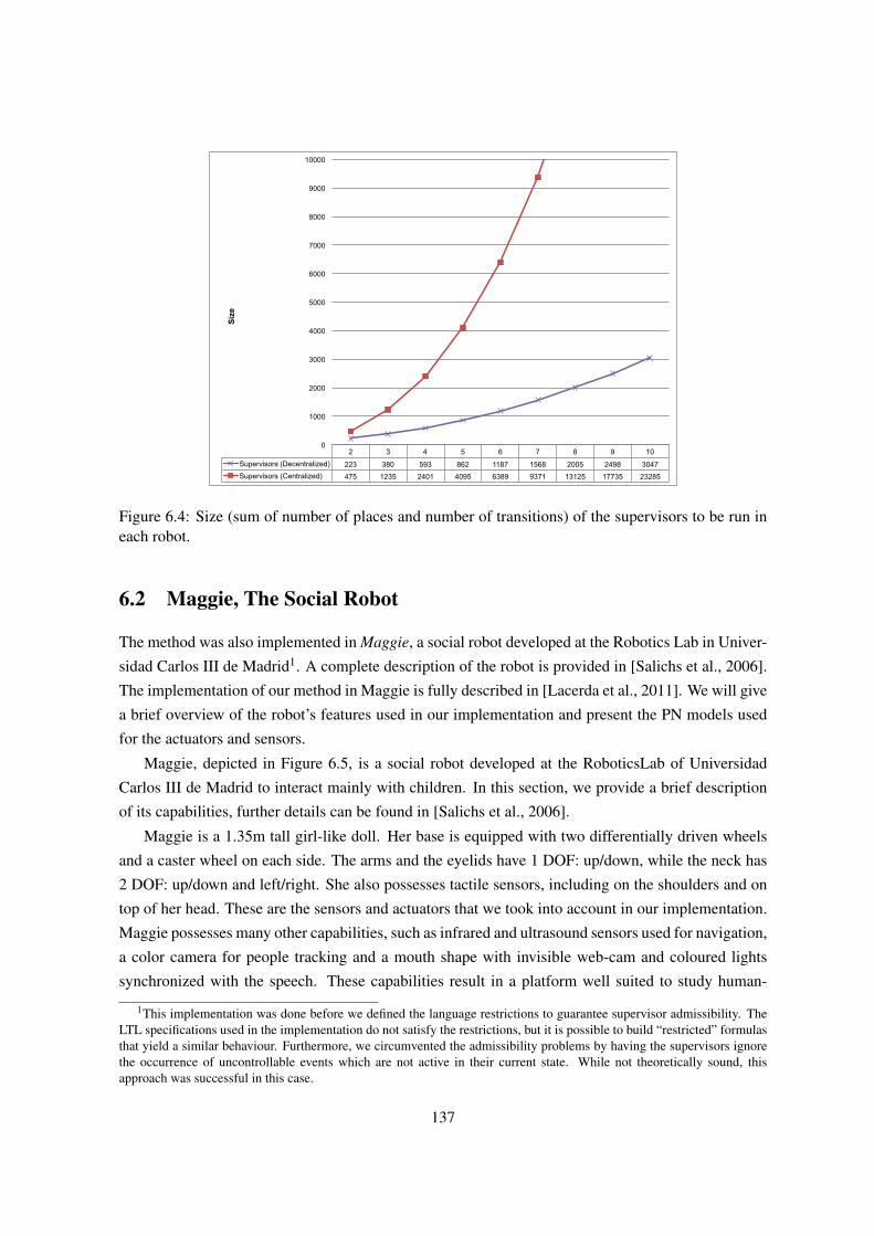
2 3 4 5 6 7 8 9 10 Supervisors (Decentralized) 223 380 593 862 1187 1568 2005 2498 3047 Supervisors (Centralized) 475 1235 2401 4095 6389 9371 13125 17735 23285

0

1000

2000

3000

4000

5000

6000

7000

8000

9000

10000

Size

Figure 6.4: Size (sum of number of places and number of transitions) of the supervisors to be run ineach robot.

6.2 Maggie, The Social Robot

The method was also implemented in Maggie, a social robot developed at the Robotics Lab in Univer-

sidad Carlos III de Madrid1. A complete description of the robot is provided in [Salichs et al., 2006].

The implementation of our method in Maggie is fully described in [Lacerda et al., 2011]. We will give

a brief overview of the robot’s features used in our implementation and present the PN models used

for the actuators and sensors.

Maggie, depicted in Figure 6.5, is a social robot developed at the RoboticsLab of Universidad

Carlos III de Madrid to interact mainly with children. In this section, we provide a brief description

of its capabilities, further details can be found in [Salichs et al., 2006].

Maggie is a 1.35m tall girl-like doll. Her base is equipped with two differentially driven wheels

and a caster wheel on each side. The arms and the eyelids have 1 DOF: up/down, while the neck has

2 DOF: up/down and left/right. She also possesses tactile sensors, including on the shoulders and on

top of her head. These are the sensors and actuators that we took into account in our implementation.

Maggie possesses many other capabilities, such as infrared and ultrasound sensors used for navigation,

a color camera for people tracking and a mouth shape with invisible web-cam and coloured lights

synchronized with the speech. These capabilities result in a platform well suited to study human-

1This implementation was done before we defined the language restrictions to guarantee supervisor admissibility. TheLTL specifications used in the implementation do not satisfy the restrictions, but it is possible to build “restricted” formulasthat yield a similar behaviour. Furthermore, we circumvented the admissibility problems by having the supervisors ignorethe occurrence of uncontrollable events which are not active in their current state. While not theoretically sound, thisapproach was successful in this case.

137

!"#$##"%%$&"$'%(')$%*%%+,$%%(+-...+ + ++/01+$%%(+ +

!"#$%&'$!"#$%&'()*)+, -)./%0, /&+1(%.+/)&, 20%3-, %&,/$2)(+%&+,()01,/&,-2(1%4/&5,+61,#-1,)7,+61,()*)+,/&,6#$%&,4%/03,0/718,96()#56,1771.+/:1,-)./%0, /&+1(%.+/)&;,()*)+-,</00,*1,%*01,+),21(7)($, $%&3, +%-=-, /&, +61, 6#$%&, -)./1+38, 961-1, +%-=-, $%3,/&.0#41;, *#+, &)+, 0/$/+14, +);, 6%&40/&5, :%(/)#-, 6)#-1, 4#+/1-;,2():/4/&5,$14/.%0,.%(1,7)(,1041(03,21)201;,%--/-+/&5,21)201,</+6,$)+)(, )(, .)5&/+/:1, 4/-%*/0/+/1-;, 14#.%+/)&%0, 1&+1(+%/&$1&+,>14#+%/&$1&+?;, 21(-)&%0, %--/-+%&.1;, 5/:/&5, 4/(1.+/)&-, %+,/&7)($%+/)&, 2)/&+-, /&, 2#*0/., 20%.1-;, 1+.8, 961-1, %220/.%+/)&-,&114, +), 41:10)2, -)./%0, ()*)+-, +6%+, %(1, %*01, +), *16%:1, </+6,6#$%&-,%-,2%(+&1(-,/7,&)+,211(-8,96/-,2%21(,2(1-1&+-,@%55/1;,%,()*)+/., 20%+7)($, 41:10)214, %+, A)*)+/.-B%*, 7)(, (1-1%(.6, )&,6#$%&'()*)+, -)./%0, /&+1(%.+/)&8, 961, 4/771(1&+, 41:10)214,/&+1(%.+/)&,$)4#01-,%(1,%0-),41-.(/*148,

+()*+,%-#!C1(-)&%0, ()*)+-;, -)./%0, ()*)+-;, 6#$%&'()*)+,

/&+1(%.+/)&8,,

-*! -23/45673-42+189:+8;+:<=+>=?+@8A8:BC+:@=>D9+E@=+B>+:<=B@+>E:F@=+D=9BG>=D+

:8+ B>:=@EC:+ H8@=+ ?B:<+ :<=+ <FHE>+ A=B>GI+ ?<=:<=@+ ;8@+ :<=+JF@J89=+8;+=>:=@:EB>H=>:+8@+ :@E>9HB99B8>+8;+B>;8@HE:B8>+;8@+:<=+A=>=;B:+8;+J=@;8@HB>G+GBK=>+:E9L9+8@+9=@KBC=9*+3<B9+>=?+@=EMB:N+ =>:EBM9+ :<=+ 8J=>B>G+ 8;+ E+ >=?+ ;B=MD+ 8;+ ?8@L+ :8+ D=EM+?B:<+ B99F=9+ C8>C=@>=D+ ?B:<+ :<=+ <FHE>"@8A8:+ 98CBEM+B>:=@EC:B8>*+ ->+ @=C=>:+ N=E@9I+ :<B9+ ;B=MD+ <E9+ E::@EC:=D+C8>9BD=@EAM=+ E::=>:B8>+ AN+ :<=+ ECED=HBC+ E>D+ :<=+ @=9=E@C<+C8HHF>B:B=9*+ 3<=+ <FHE>"@8A8:+ 98CBEM+ B>:=@EC:B8>+ B9+ E>+B>:=@DB9CBJMB>E@N+ ;B=MDI+ ?<BC<+ B>:=G@E:=9+ 9N>=@GBCEMMN+@8A8:BC9I+ E@:B;BCBEM+ B>:=MMBG=>C=I+ C8G>B:BK=+ 9CB=>C=I+J9NC<8M8GN+E>D+8:<=@+;B=MD9+MBL=+MB>GFB9:BC9+E>D+=@G8>8HBC9I+B>+ 8@D=@+ :8+ BHJ@8K=+ :<=+ >E:F@EM>=99+ 8;+ <FHE>"@8A8:+B>:=@EC:B8>*+1E>N+ @8A8:BC+ JME:;8@H9+ <EK=+ A==>+ AFBM:+ ?B:<+ DB;;=@=>:+

D=9BG>+C8>9BD=@E:B8>9+E>D+CEJEABMB:B=9+:8+9:FDN+<FHE>"@8A8:+98CBEM+B>:=@EC:B8>*+OB9H=:+B9+E>+=PJ@=99BK=+E>:<@8J8H8@J<BC+@8A8:+ <=ED+ D=K=M8J=D+ E:+ 1-3+ ?B:<+ J=@C=J:FEM+ E>D+ H8:8@+H8DEMB:B=9+ :EBM8@=D+ :8+ >E:F@EM+ <FHE>+ C8HHF>BCE:B8>+C<E>>=M9+Q!R*+3<B9+@8A8:+<E9+A==>+D=9BG>=D+:8+E99B9:+@=9=E@C<+B>:8+ 98CBEM+ B>:=@EC:B8>9+ A=:?==>+ @8A8:9+ E>D+ <FHE>9*+ SBL=+OB9H=:I+ TJE@LN+ B9+ 98CBEM+ @8A8:+ :<E:+ F9=9+ A8:<+ ;ECBEM+=PJ@=99B8>+E>D+H8K=H=>:+:8+B>:=@EC:+?B:<+<FHE>9+Q$R*+/6U-+B9+ E>8:<=@+ E>:<@8J8H8@J<BC+ @8A8:+ ?B:<+ E+ <=ED+ E>D+ E@H9+D=9BG>=D+;8@+@=9=E@C<+8>+@=EM":BH=+98CBEM+B>:=@EC:B8>+A=:?==>+

@8A8:9+ E>D+ <FHE>9+ QVR*+ 0+ /8A8:E+ B9+ E+ 98J<B9:BCE:=D+=DFCE:B8>EM+ :8N+ @8A8:+D=9BG>=D+ :8+AFBMD+<FHE>"@8A8:+ 98CBEM+B>:=@EC:B8>9+ ?B:<+ C<BMD@=>+ ?B:<+ H8:8@+ E>D+ C8G>B:BK=+DB9EABMB:B=9+Q#R*+->+:<=+SB>8+J@8W=C:I+E+@8A8:+<=ED+?B:<+E+>BC=I+CF:=+EJJ=E@E>C=+ E>D+=H8:B8>EM+ ;==DAECL+CE>+A=+C8>;BGF@=D+B>+9FC<+E+?EN+:<E:+:<=+<FHE>+F9=@+=>W8N9+:<=+B>:=@EC:B8>+E>D+?BMM+ H8@=+ =E9BMN+ ECC=J:+ J899BAM=+ HB9F>D=@9:E>DB>G9+ Q&R*+1EGGB=+ B9+ E+ 98CBEM+ @8A8:+ D=K=M8J=D+ E:+ /8A8:BC9SEA+ E>D+ B9+D=9C@BA=D+B>+:<=+J@=9=>:+JEJ=@+XYBGF@=+!Z*++

+

+

YBG*+!+/8A8:BC9SEA[9+1EGGB=+

->9:=ED+ 8;+ F9B>G+H=C<E>BCEM+ EC:FE:B8>I+ 8:<=@+ 98CBEM+ @8A8:+J@8W=C:9+ @=MN+ 8>+ C8HJF:=@+ G@EJ<BC9+ E>D+ E>BHE:B8>+:=C<>B\F=9*+]BLBEI+;8@+=PEHJM=I+<E9+E+V5+@=>D=@=D+;EC=+8;+E+?8HE>I+ ?<BC<+ J=@HB:9+ HE>N+ D=G@==9+ 8;+ ;@==D8H+ ;8@+G=>=@E:B>G+ =PJ@=99B8>9+ Q(R*+ ]EM=@B=+ /8A8C=J:B8>B9:+ Q^RI+_/07.+ X_@EDFE:=+ /8A8:+ 0::=>DB>G+ E+ 78>;=@=>C.Z+ E>D+_=8@G=+Q`R+E@=+E>8:<=@+=PEHJM=9+;8@+C8HJF:=@+G@EJ<BC"AE9=D+98CBEM+ @8A8:9I+ ?<BC<+ <EK=+ =PJ@=99BK=+ ;EC=9+ 8>+ JE>>B>G+JME:;8@H9+ E9+ ?=MM+ E9+ ME@G=+ E@@EN+ 8;+ 9=>98@9*+ ]EM=@B=+/8A8C=J:B8>B9:+<E9+A==>+D=K=M8J=D+:8+B>K=9:BGE:=+M8>G":=@H+

1EGGB=a+0+/8A8:BC+bME:;8@H+;8@+cFHE>"/8A8:+T8CBEM+->:=@EC:B8>+

1BGF=M+0*+TEMBC<9I+/EHd>+UE@A=@I+0MEE+1*+O<EHB9I+1E@eE+1EM;EfI+gEKB=@+Y*+_8@89:BfEI+/EL=M+bEC<=C8I+/E;E=M+/BKE9I+0>E+78@@EM=9I+.M=>E+5=MGED8I+5EKBD+_E@CeE+/8A8:BC9SEAI+5=JE@:H=>:+8;+TN9:=H9+.>GB>==@B>G+E>D+0F:8HE:B8>+

7E@M89+---+6>BK=@9B:N+1ED@BDI+TJEB>

Figure 6.5: Maggie, the social robot, interacting with a child.

robot interaction and robot learning by training and teaching.

The control architecture is based on the automatic-deliberative (AD) control architecture proposed

in [Barber and Salichs, 2001]. In this architecture, the robot skills are divided in two levels. In the

automatic level, we find the skills related with robot sensors and actuators. In the deliberative level,

we find higher-level skills, such as a planner or our implementation of the feedback-loop of SC. The

skill we developed subscribes to events representing changes in sensor readings, for which an event

handler is implemented. Also, it can order the execution of skills related to performing simple actions

(e.g., raising an arm or start spinning).

We will use PNs to model Maggie behaving freely in the environment. In the PN models used

here both places and transitions have a specific interpretation:

• Places represent the value of binary variables that are used to define the state of the system, i.e.,

all places correspond to the truth value of some state description symbol;

• Transitions represent orders to execute actions or changes in sensor readings, i.e., the firing of a

transition represents a communication between our implementation and the automatic level of

the architecture.

In Figure 6.6 we depict the PN model for Maggie. Contrary to the other examples, where the

individual models already have some structure, representing the basic behaviour of each robot, and

we use LTL to specify coordination rules for the team, in this case we start with a very unstructured

model, where the robot can perform any of its available actions randomly, and use the LTL formulas

to restrict the available actions so that a given behaviour is achieved.

We note that, for the base, when a start action is issued, the robot starts performing that action

138

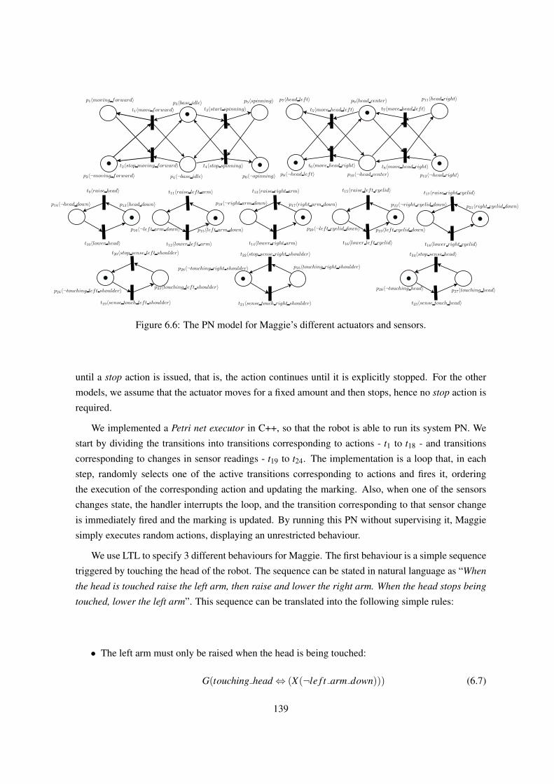
Figure 6.6: The PN model for Maggie’s different actuators and sensors.

until a stop action is issued, that is, the action continues until it is explicitly stopped. For the other

models, we assume that the actuator moves for a fixed amount and then stops, hence no stop action is

required.

We implemented a Petri net executor in C++, so that the robot is able to run its system PN. We

start by dividing the transitions into transitions corresponding to actions - t1 to t18 - and transitions

corresponding to changes in sensor readings - t19 to t24. The implementation is a loop that, in each

step, randomly selects one of the active transitions corresponding to actions and fires it, ordering

the execution of the corresponding action and updating the marking. Also, when one of the sensors

changes state, the handler interrupts the loop, and the transition corresponding to that sensor change

is immediately fired and the marking is updated. By running this PN without supervising it, Maggie

simply executes random actions, displaying an unrestricted behaviour.

We use LTL to specify 3 different behaviours for Maggie. The first behaviour is a simple sequence

triggered by touching the head of the robot. The sequence can be stated in natural language as “When

the head is touched raise the left arm, then raise and lower the right arm. When the head stops being

touched, lower the left arm”. This sequence can be translated into the following simple rules:

• The left arm must only be raised when the head is being touched:

G(touching head⇔ (X(¬le f t arm down))) (6.7)

139

• The right arm must only be raised after the left arm is raised:

G(raise le f t arm⇔ (Xraise right arm)) (6.8)

• After raising the right arm, it must be immediately lowered again:

G(raise right arm⇒ (Xlower right arm)) (6.9)

The second behaviour shows how to specify different reactions to different sensor readings. We

can state it has “If the left shoulder is touched, wait until the right shoulder is touched and then raise

your right arm. If the right shoulder is touched, wait until the left shoulder is touched and raise

your left arm. After raising an arm, lower it again and return to the initial state”. To keep track of

which shoulder is touched, we use the state of the eyelids. If both eyelids are down, then no shoulder

has been touched yet. If one of the eyelids is up, then the corresponding shoulder was touched and

Maggie is waiting for the other shoulder to be touched. Hence, the behaviour can be implemented by

the following rules:

• If the left shoulder is touched and both eyelids are down (i.e., no shoulder was touched yet),

raise the left eyelid:

G((sense le f t shoulder∧ right eyelid down∧ le f t eyelid down)⇔ (Xraise le f t eyelid))(6.10)

• If the right shoulder is touched and the left eyelid is up (i.e., the left shoulder was previously

touched), raise the right arm:

G((sense right shoulder∧¬le f t eyelid down)⇔ (Xraise right arm)) (6.11)

• After raising the right arm, return to the initial state by lowering the left eyelid and the right

arm:

G(raise right arm⇔ (Xlower le f t eyelid)) (6.12)

G(lower le f t eyelid⇔ (Xlower right arm)) (6.13)

• If the right shoulder is touched and both eyelids are down (i.e., no shoulder was touched yet),

raise the right eyelid:

G((sense right shoulder∧ right eyelid down∧ le f t eyelid down)⇔ (Xraise right eyelid))(6.14)

• If the left shoulder is touched and the right eyelid is up (i.e., the right shoulder was previously

140

touched), raise the left arm:

G((sense le f t shoulder∧¬right eyelid down)⇔ (Xraise le f t arm)) (6.15)

• After raising the left arm, return to the initial state by lowering the right eyelid and the left arm:

G(raise le f t arm⇔ (Xlower right eyelid)) (6.16)

G(lower right eyelid⇔ (Xlower le f t arm)) (6.17)

Note that in this behaviour, touching the same shoulder more than one time in a row does influence

the arm to be raised. After touching one of the shoulders, Maggie ignores all other sensor readings

until the other shoulder is touched. When that happens, she raises the corresponding arm.

The third behaviour is also triggered by touching the head, but we allow the robot to perform

random actions during the behaviour. It can be stated as “Move arms randomly. When the head is

touched, start spinning until both arms are up”. This can be translated into the following rules:

• Only start spinning when the head is touched, you are not spinning yet and both arms are not

already up:

G((sense head∧ (¬spinning)∧¬(¬le f t arm down∧¬right arm down))⇔(Xstart spinning))

(6.18)

• After starting to spin, continue spinning until both arms are up:

G(start spinning⇒ (X(spinningU(¬le f t arm down∧¬right arm down)))) (6.19)

• When both arms are up, stop spinning (or continue stopped if you are not spinning):

G(¬le f t arm down∧¬right arm down)⇒ (X¬spinning)) (6.20)

All of these examples also include an additional formula which avoids the execution of the actions

that are not referred to in the specification, i.e., in each example, a formula of the form G(∧

e∈Eo¬e),

where Eo is the set of actions that is not mentioned in that example is also added.

In the video available at http://youtu.be/D3EwqAEE268, we show both the uncontrolled be-

haviour of Maggie and its behaviour when being supervised by the PNs obtained from the specifica-

tions described here.

141

http://youtu.be/D3EwqAEE268

Figure 6.7: The e-puck robot (re-printed from [Mondada et al., 2009]).

6.3 Surveillance Scenario with E-Pucks

In this section, we describe the larger scale implementation of out methodology. This was an imple-

mentation of a surveillance scenario in a team of real mobile robots. We will start by discussing the

scenario implementation details, and then show the LTL rules used for the coordination.

6.3.1 Scenario Description

We implemented this scenario using the e-puck robots [Mondada et al., 2009]. The e-puck (Figure 6.7)

is a small circular, differential driven robot, with 7cm of diameter, 6cm of height and 660g, developed

at the Ecole Polytechnique Federale de Lausanne.

More details about the robot can be found in its homepage http://www.e-puck.org/. Given

that our goal was to test the high-level LTL specifications, we only used the e-pucks for navigation,

using an overhead camera for both robot localization and event detection. Before describing the set-

up, we show the scenario, which is a 2.1m×1.6m rectangular representation of a floor, composed of

an inner corridor and 10 rooms, as depicted in Figure 6.8.

The goal is to have a team of 4 e-pucks doing surveillance in the scenario, looking for 3 different

anomalous situations, which we will represent by different coloured rectangles in the rooms2:

1. A dirty room, represented by a blue rectangle;

2. An abandoned object, represented by a green rectangle;

3. A fire, represented by a red rectangle.

As we already stated, we use an overhead AXIS P13 camera for both individual robots localization

and room events detection. Furthermore, we use a central computer to process the images, run the PN

supervisors and send move commands to the e-pucks, by Bluetooth wireless communications. Figure

6.9 depicts a diagram of the different modules used.

We give a brief overview on each of the modules. We used the robot operating system (ROS) to

manage the camera drivers and the messages passed between different modules:2We assume that the anomalous situations can only occur inside the rooms.

142

http://www.e-puck.org/

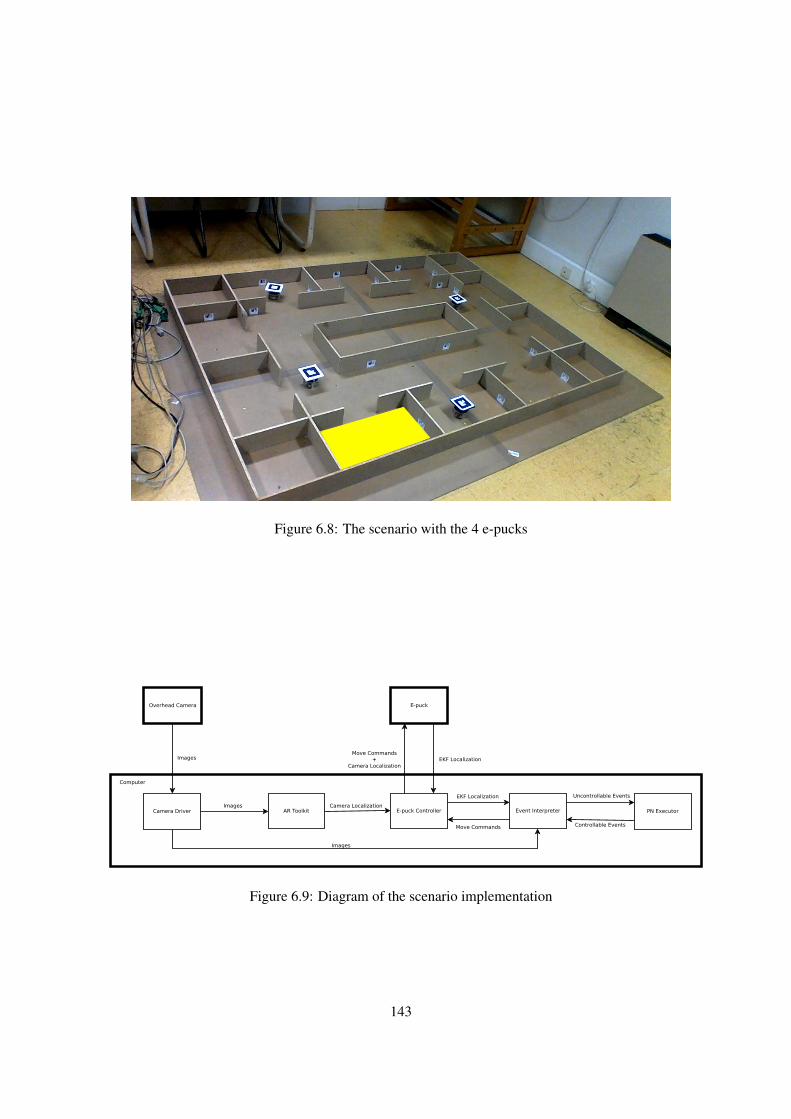
Figure 6.8: The scenario with the 4 e-pucks

Figure 6.9: Diagram of the scenario implementation

143

• The AXIS P13 camera retrieves images of the whole scenario and sends them to the central

computer by cable Ethernet;

• In the computer, the ROS camera driver receives the image stream and publishes it in a ROS

topic;

• In the computer, ARToolKit3 [Kato and Billinghurst, 1999] subscribes to the image topic and is

used to get a 3D position for each robot, which is translated to 2D via a simple projection. To

use ARToolkit, we placed a small marker on top of each e-puck, which is used both to identify

the robot and to find its orientation. The values (x,y,θ) for each robot are then published in

another ROS topic;

• In the computer, the e-puck controller subscribes to the topic published by ARToolKit, and

also receives move and stop commands from the PN executor. Both the camera positions and

the commands are sent to the e-pucks via bluetooth. Furthermore, the e-puck controller also

receives, via Bluetooth, updated positions from the e-pucks and publishes them in a ROS topic;

• The e-pucks execute the move commands received from the e-puck controller and run an ex-

tended Kalman filter (EKF) using their odometry and the ARToolkit localization data to update

their localization. This approach is used to mitigate camera localization errors, the camera de-

lay, and to reduce the communication frequency between the central computer and the e-pucks,

thus avoiding latency in the Bluetooth network;

• The event interpreter subscribes to the e-puck localizations topic and the image topic, and uses

its information to compute the uncontrollable events that occurred. The image topic is used

to fire the room events (using a simple color detection algorithm) and the e-puck localization

is used for all other uncontrollable events, which have a relation to the e-puck positions. For

example, if robot i is inspecting a room and the camera detected a blue rectangle in the room

corresponding to the position of robot i, then uncontrollable event f ound dirty roomi is fired.

It also receives controllable events from the PN executor and transforms them into move com-

mands to be sent for the robot. For example, if the fired event is continue in corridori, it

computes the point in front of the next door and creates a move command to be sent for robot i,

with that position as the goal.

• The PN executor is used to run the PN supervisors. It receives the uncontrollable events from

the event interpreter and fires them immediately, updating the states of the supervisors, and also

randomly chooses controllable events enabled by all supervisors to be fired, also updating the

supervisors states. When all the controllable events are disabled, it waits for a new uncontrol-

lable event to be fired and change the PN supervisors state.

3The choice for ARToolKit was due to its integration in ROS.

144

The overhead camera detects the room events. However, we simulate that these detections are

made by the robots. In fact, initially we started by using the e-puck on-board cameras for color

detection, but this approach was less reliable, and also made the occurrence of these events harder to

understand in the videos. This happened because we needed to put the rectangles standing in front of

the e-pucks, which did not make them very visible in the overhead camera video. Thus, a room event

is only detected when a robot is in the room where that event has occurred.

6.3.2 PN Models and LTL Specifications

We now proceed to the high-level task implementation details. Our decision for this example was

to modularly model the individual robot basic behaviours using PNs with algebraic state description,

and to use LTL to specify in which situations a given behaviour should be executed. We start by

describing the individual robot possible behaviours. The PN models for these behaviours are presented

in Appendix A. Each robot is able to:

• Move (counter-clockwise) around the corridor, stopping whenever a new room door is found;

• When in front of a room door, randomly decide whether to enter room or continue;

• Go (directly) to a special security room – the room in yellow in Figure 6.8;

• When inside the special security room, leave it;

• Go towards a teammate position;

• When a dirty room is found, clean it;

• When an abandoned object is found, pick it up;

• When holding an object, drop it;

• When a fire is detected, extinguish it;

• When a room is clear, leave it.

We will simulate some of these behaviours in the following way:

• While cleaning a room, the robot simply stands still until the room is clean (i.e., the blue rect-

angle is removed) or it decides to stop cleaning the room;

• Picking an object just changes the PN marking, the robot does not do anything. Whenever a

robot picks up an object, we will remove the green rectangle

• When a robot starts extinguishing a fire, it moves to one of the sides of the room, if one is

available (to allow other robots to enter the room). It then simply stands still until the fire is

extinguished (i.e., the red rectangle is removed) or it decides to stop extinguishing the fire.

145

In the video showing a run of the system we will use color codes on top of the robots to allow the

viewer to understand what each robot is doing.

Note that the first two behaviours are the “default” behaviours for the robot, and are executed

whenever none of the other behaviours is being executed. Also, while some of the behaviours, such as

extinguishing a fire, can only occur when a fire is detected, initially we allow the robots to randomly

choose to go to the special security room or towards a teammate. The LTL formulas will be used

to specify when these behaviours should be executed, and when they should be stopped. The list of

natural language specifications we want the system to fulfil, and its translations to LTL formulas4 is

the following:

• Spread around the scenario: For each robot i, if it just passed in front of a room that has another

robot inside, it must not enter other rooms until it passes in front of at least 2 rooms without

entering or it starts moving towards a teammate5:

G(room occupiedi⇒ (X(¬start entering roomiW

(M(rooms passedi)≥ 2∨∨j 6=i

start going towards teammate j,i)))) (6.21)

• Avoid spending too much time without checking rooms: For each robot i, if it passes in front of

2 or more rooms without entering, and the current room is not occupied, do not continue in the

corridor:

G((M(rooms passedi)≥ 2∧¬room occupiedi)⇒ (X¬continue in corridori)) (6.22)

• For each robot i, only go to the safe room if it is holding a bag:

G(¬holding bagi⇒ (X¬start going to sa f e roomi)) (6.23)

• For each robot i, only drop a bag it is holding if it is in the safe room:

G(¬in sa f e roomi⇒ (X¬drop bagi)) (6.24)

• For each robot i, never leave the safe room if it is holding a bag:

G(holding bagi⇒ (X¬start leaving sa f e roomi)) (6.25)

4To facilitate the reading of the formulas, for places with bound 1, we will write p instead of M(p) ≥ 1 (which isequivalent to M(p) = 1, i.e., “p is satisfied”) and ¬p instead of M(p)≥ 1, i.e., “p is satisfied”.

5We also reason about the robot starting moving towards a teammate in this case because moving towards a teammateimplies entering the room where the teammate is. Thus, if we do not include this condition and the robot starts movingtowards a teammate after passing in front of an occupied room, it will not be able to enter the room where the teammate is,because it would falsify the specification.

146

• If robot i is not next to a fire, then no other robots should go towards it:

G(¬next to f irei⇒ (X∨j 6=i

¬start going towards teammatei, j)) (6.26)

• If there is not a fire, then the robots should not stop cleaning dirty rooms:

G(¬ f ire⇒ (X∧

i

¬stop cleaning roomi)) (6.27)

• For each robot i, if it is next to a fire, then the other robots should not stop going towards it:

G(next to f irei⇒ (X∨j 6=i

¬stop going towards teammatei, j)) (6.28)

• For each robot i, no more than two teammates should move towards it (there can be a maximum

number of 3 robots in each room, due to space constraints)

G∑j 6=i

M(going towards teammatei, j)≤ 2 (6.29)

• There should not be more that one robot going towards the safe room at each time (to avoid

collisions between robots in that room)

G∑i

M(going to sa f e roomi)≤ 1 (6.30)

A video showing a run of the robots that satisfies this set of rules is available at http://youtu.

be/3sOEYxdDjFA. Note that one can change the behaviour of the team easily by simply changing

some of these rules. Thus makes the addition of new behaviours easy. For example, if we assume that

the robots cannot extinguish fires, one could simply delete all the “fire related” rules and allow the

robot to go to the security room to warn a human also when it detects a fire.

147

http://youtu.be/3sOEYxdDjFA

http://youtu.be/3sOEYxdDjFA

CHAPTER 7

Conclusions and Further Work

7.1 Conclusions

In this thesis, we described methodologies to build an FSA or PN realization of a supervisor that is

guaranteed by construction to restrict the behaviour of an uncontrolled system (modelled as an FSA

or a PN, respectively) so as to fulfil an LTL specification. The similarities between natural language

and temporal logic, and the fact that we can write formulas over both the events of the system and

a set of atomic propositions used to describe the states, allow us to build supervisors that realize

intricate/complex behaviours that are guaranteed by construction to be consistent with the temporal

logic specification. These methods provide the designer with a framework that requires him/her to:

1. Model the system as an FSA or PN;

2. Specify the intended behaviour for the system as a set of LTL formulas.

FSA and PN are two suitable, well known and well accepted frameworks to model robot tasks.

Also, LTL is a suitable, well known and well accepted formalism to reason about properties of a

system (hence, to synthesize supervisors that fulfil those properties). Therefore, the combination of

the two leads to methodologies that reduce design errors, and enable the implementation of larger and

more complex systems, from the modular composition of simple models and specifications.

We illustrated the application of the methodologies using a simulated multi-robot scenario, an

implementation on a real social robot and a real multi-robot surveillance scenario. From these exper-

iments, we draw the following conclusions:

• the use of LTL (written over the set of events plus symbols describing the state of the world) as

the specification language enables one to bridge the gap between a natural language specifica-

tion for a robot system and a supervisor that enforces it;

149

• the use of FSA models induces very large supervisors for multi-robot systems, due to the need

to enumerate all the possible states of a heavily distributed system;

• PN models are more suited for the modelling of multi-robot systems, due to the distributed

nature of PN state representation (i.e., markings). The advantage of using PNs is twofold,

facilitating the task of the designer and also inducing smaller supervisors, thus improving the

computational efficiency of the method;

• a further improvement to the computational efficiency of the methodologies described here is

defining a decentralized version, where we simply augment the PN models of each robot such

that they are able to handle communication between each other.

These experiments, in particular the multi-robot surveillance scenario, also show the application

of SC theory in an mobile multi-robot scenario of a considerable size. This is another important

contribution of this work. However, the implementation of this scenario also showed some of the lim-

itation of the approach when dealing with intelligent robot systems. These limitations are due to two

main reasons: the difficulty between mapping the robot’s sensor readings into the occurrence of un-

controllable events and the lack of ability to handle uncertainty. In the next section, where we discuss

further work, we will provide a possible research route to mitigate these limitations. Furthermore, we

also note that these limitations are inherent to the application of SC theory in this field, and the main

goal of this thesis was to provide a general framework for the use of LTL specifications in SC of DES

modelled as PNs.

7.2 Further work

Our introduced methods constitute a novel approach to the SC of PNs. Moreover, the theory for

SC of PNs is still not completely studied. Thus, there is a significant amount of open problems and

improvements that can be subject of future work.

• Dealing with dead transitions in the BA/PN system model composition. As referred is Section

4.2.2, since the BA/PN system model composition is based on analysing the PN structure,

without building the reachability graph, some transitions are created that are never active in

the reachable markings of the PN resulting from the composition. These dead transitions do

not affect the behaviour of the system, but their deletion is desirable because they increase the

size of the model and, as seen in Section 6.2, there can be a large amount of dead transitions.

This larger size of the model has an impact on analysis and also on execution, because there

are transitions that can never be active but nonetheless are checked at each step of the feedback

loop. The simple approach we presented already deletes a large percentage of dead transitions,

but more effective approaches should be used. In a complementary approach to solve this

problem, it might be possible that one can detect at least a subset of the dead transitions during

the composition, and this will be investigated.

150

• We presented the use of a knowledge base K for PN system models with symbolic state de-

scription that provides extra information which allows for smaller supervisors. We briefly men-

tioned that PN analysis techniques can be used to create the knowledge base, but the version

we presented still relies on the designer writing information that he knows is true in all reach-

able markings of the PN. Creating knowledge bases automatically from the PN structure using

invariant analysis, and extending the notion of knowledge base for PN system models with

algebraic state description will be subject of future work.

• Modular supervision for systems generating ω-languages has not been studied in the literature.

In particular, it is relevant to define methodologies to check deadlock-freeness under modular

supervision without composing all the supervisors (thus effectively ruling out the argument for

using modular SC). In our case, since the specifications are initially given in LTL, it would be

useful to find a way of checking the different formulas used for each specifications and guaran-

tee that their conjunction does not originate deadlock situations. We believe it is possible to do

this using the BA obtained from the formulas. Furthermore, generalizing deadlock prevention

algorithms so that they can deal with the concurrent execution of a set of PNs might be both

interesting from a theoretical point-of-view, and to provide a more efficient solution for the

problem.

• Studying the class of deterministic PN languages generated by our approach. In Section 5.2.2,

when discussing how to apply the standard algorithm for checking admissibility for our method-

ology, we considered G as a deterministic PN representation of the system behaviour, and

G ‖ Gϕ as the deterministic PN language specification. Thus, we argued that our methodol-

ogy can be seen as a way to create deterministic PN language specifications, in the style of

the Ramadge-Wonham framework. This raises a set of interesting questions which are worth

being studied, e.g., what is the class of deterministic PN languages that can be specified using

syntactically safe LTL and PN system models with algebraic state description?

• Given that the result of the BA/system model composition always has a substructure that repre-

sents the determinization of the BA, it is expectable that taking the properties of that substruc-

ture into account (e.g., at any marking one and only one place of the Buchi determinization

will be marked) one can improve the computational efficiency of the algorithms for checking

admissibility and deadlock-freeness. It might also be possible that the substructure can help in

trimming the composition so that in becomes deadlock-free and admissible.

• An important result of Section 5.2.2 is that we are able to represent all the markings which

are deadlocked or uncontrollable in a finite structure. The goal now will be to take advantage

of this structure to create approaches that ensure admissibility and deadlock-freeness of the

supervisor. The marking-based control-laws are the most direct approach to do this, but there

might be others.

151

• Given the difficulty on handling arbitrary PNs, we can consider special classes of PN (e.g.,

workflow nets, free-choice nets, etc.) and use their properties to improve the algorithms for ad-

missibility and deadlock-freeness. Furthermore it would be interesting to analyse which classes

of PNs are closed for the BA/system model composition.

• One can also define an equivalent approach for other classes of LTL. The safety fragment of

LTL is quite well-behaved and the more attentive reader will notice that all the big challenges in

this methodology stem from the use of PNs. However, we can also think of increasing the ex-

pressibility of the LTL specifications. One immediate class of LTL formulas that can be worked

on is the class of co-safe languages, i.e., languages which are the complement of safe languages.

These languages are also accepted by deterministic BA, and they have a single accepting state

which, once the reached for the first time, cannot be exited anymore. Furthermore, after the

accepting state is reached, all the labels of the BA alphabet become enabled. Thus, we can

use co-safe LTL formulas to specify reachability behaviours. However, guaranteeing that the

accepting state of the BA is eventually reached in finite time for all the executions of the system

will require extra operations on the composition.

• The decentralized approach presents a large set of opportunities to extend our proposals:

– Define a way to incorporate shared description symbols in the specification;

– Allow the designer to write global specifications, which are then satisfied locally and in a

decentralized way;

– Abstract the id’s of the robots when that is possible;

– Extend the approach to system models with algebraic state description;

– Framing this decentralization methodology within the existing theory of distributed SC

can be studied.

• A final and particularly interesting direction of further work in the context of intelligent robot

systems is related to adding uncertainty to the models. The methodologies we presented are

purely qualitative, which can be seen as a limitation in the context of robotics, where there is

an inherent uncertainty about the state of the world that stems from sensor’s inaccuracy. Thus,

adding uncertainty to the models is both interesting in theoretical terms and has a very good

motivation in terms of the method’s applicability. One particularly interesting idea for future

work is using generalized stochastic Petri nets (GSPN) [Viswanadham and Narahari, 1992] to

model the systems and take advantage of recent work that connects GSPN models with inter-

active Markov chains (IMC) [Katoen, 2012]. The IMCs can then be analysed, using recent

developments in the analysis of real-time stochastic games to obtain several quantitative objec-

tives such as expected time to reach a marking, time spent in a given marking in the long run,

or time-bounded reachability objectives. Furthermore, these analysis tools yield marking based

policies that minimize or maximize each of these objectives, or a mix between them. Given this,

152

it is our claim that these approaches can be further investigated to see how one can find poli-

cies that maximize the probability of satisfying objectives given in LTL, i.e., we can adapt this

approach to also do planning. Also, one can use modelling and identification approaches using

GSPNs and specially tailored for robot systems, e.g., [Costelha and Lima, 2012]. Thus, when

working towards making our methodology more applicable in robot systems, this direction is

very relevant.

The fact that so many new challenges arose from this work also indicates that this line of research

has the potential for improvement, being a relevant topic to be further tackled.

153

Appendices

155

APPENDIX A

PN Models for the Surveillance Scenario

We present the PN models used for the implementation described in Section 6.3. In the end od the

appendix, we also list the set of uncontrollable events for robot i. All the places in the models have

bound 1, except for places rooms passedi and rooms passedi, which have bound 10.

157

Figure A.1: PN model for the surveillance behaviour while in the corridor. Note that t5 is in factrepresenting 10 transitions, one for each k = 1, ...,10 (to represent this we also but the correspondingarcs with weight k in bold, to depict the representation of 10 arcs). Each transition tk

5 is enabled if andonly if place rooms passedi has exactly k tokens. This structure can be easily implemented in a PN.The place pausedi has reflexive arcs for all the transitions, i.e., they can only be active when there isa token in pausedi. To improve readability, we depict this by putting the place in bold.

Figure A.2: PN model for the teammate avoidance behaviour.

158

Figure A.3: PN model for the room inspection behaviour.

Figure A.4: PN model for the room cleaning behaviour.

159

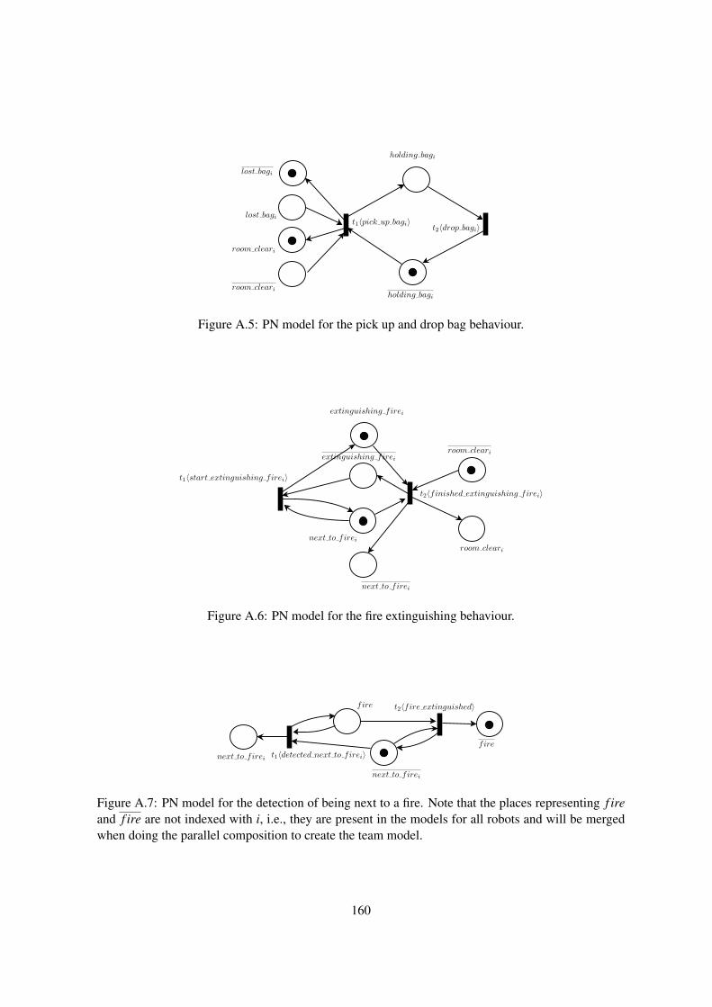
Figure A.5: PN model for the pick up and drop bag behaviour.

Figure A.6: PN model for the fire extinguishing behaviour.

Figure A.7: PN model for the detection of being next to a fire. Note that the places representing f ireand f ire are not indexed with i, i.e., they are present in the models for all robots and will be mergedwhen doing the parallel composition to create the team model.

160

Figure A.8: PN model for moving behaviour when inside a room.

161

Figu

reA

.9:P

Nm

odel

fort

hem

ovin

gto

war

dssa

fero

ombe

havi

our.

162

Figu

reA

.10:

PNm

odel

fort

hem

ovin

gto

war

dste

amm

ate

j.N

ote

that

fore

ach

robo

ti,w

eha

ven−

1of

thes

em

odel

s,w

here

nis

the

tota

lnum

ber

ofro

bots

onth

ete

am.

163

Uncontrollable events for robot i:

room entrance f oundi room emptyi room occupiedi

f inished cleaning roomi detected next to f irei f ire extinguished

f ound dirty roomi f ound lost bagi f ound f irei

f ound room cleari f inished extinguishing f irei f inished entering roomi

f inished leaving roomi f ound teammatei lost teammatei

f inished leaving sa f e roomi sa f e room entrance f oundi f inished entering sa f e roomi

f inished going towards teammate j,i teammate j room entrance f oundi

164

Bibliography

[Abdulla et al., 2004] Abdulla, P. A., Iyer, S., and Nylen, A. (2004). SAT-solving the coverability

problem for Petri nets. Formal Methods in System Design, 24(1):25–43.

[Alpern and Schneider, 1987] Alpern, B. and Schneider, F. (1987). Recognizing safety and liveness.

Distributed computing, 2(3):117–126.

[Asın et al., 2011] Asın, R., Nieuwenhuis, R., Oliveras, A., and Rodrıguez-Carbonell, E. (2011). Car-

dinality networks: a theoretical and empirical study. Constraints, 16(2):195–221.

[Aydin Gol et al., 2012] Aydin Gol, E., Lazar, M., and Belta, C. (2012). Language-guided controller

synthesis for discrete-time linear systems. In Proceedings of the 15th ACM international confer-

ence on Hybrid Systems: Computation and Control, pages 95–104, Beijing, China. ACM.

[Barber and Salichs, 2001] Barber, R. and Salichs, M. (2001). A new human based architecture for

intelligent autonomous robots. In Proceedings of the The Fourth IFAC Symposium on Intelligent

Autonomous Vehicles, pages 85–90, Sapporo, Japan.

[Basile et al., 2006] Basile, F., Chiacchio, P., and Giua, A. (2006). Suboptimal supervisory control

of petri nets in presence of uncontrollable transitions via monitor places. Automatica, 42(6):995–

1004.

[Belta et al., 2007] Belta, C., Bicchi, A., Egerstedt, M., Frazzoli, E., Klavins, E., and Pappas, G.

(2007). Symbolic planning and control of robot motion [grand challenges of robotics]. IEEE

Robotics & Automation Magazine,, 14(1):61–70.

[Cassandras and Lafortune, 2006] Cassandras, C. G. and Lafortune, S. (2006). Introduction to Dis-

crete Event Systems. Springer-Verlag New York, Inc., Secaucus, NJ, USA.

[Chen et al., 2012a] Chen, C.-H., Kuo, C.-M., Chen, C.-Y., and Dai, J.-H. (2012a). The design and

synthesis using hierarchical robotic discrete-event modeling. Journal of Vibration and Control.

165

[Chen et al., 2012b] Chen, Y., Tumova, J., and Belta, C. (2012b). LTL robot motion control based

on automata learning of environmental dynamics. In Procedings of ICRA ’12: The 2012 IEEE

International Conference on Robotics and Automation, pages 5177–5182, St. Paul, MN, USA.

IEEE.

[Chen et al., 2000] Chen, Y.-L., Lafortune, S., and Lin, F. (2000). Design of nonblocking modular

supervisors using event priority functions. IEEE Transactions on Automatic Control, 45(3):432–

452.

[Cheng et al., 1993] Cheng, A., Esparza, J., and Palsberg, J. (1993). Complexity results for 1-safe

nets. In Foundations of software technology and theoretical computer science, pages 326–337.

Springer.

[Cimatti et al., 2002] Cimatti, A., Clarke, E., Giunchiglia, E., Giunchiglia, F., Pistore, M., Roveri,

M., Sebastiani, R., and Tacchella, A. (2002). Nusmv 2: An opensource tool for symbolic model

checking. In Proceedings of CAV ’02: The 14th International Conference on Computer Aided

Verification, pages 241–268, Copenhagen, Denmark. Springer.

[Cimatti et al., 2003] Cimatti, A., Pistore, M., Roveri, M., and Traverso, P. (2003). Weak, strong, and

strong cyclic planning via symbolic model checking. Artificial Intelligence, 147(1–2):35 – 84.

[Cizelj and Belta, 2013] Cizelj, I. and Belta, C. (2013). Control of noisy differential-drive vehicles

from time-bounded temporal logic specifications. In Procedings of ICRA ’13: The 2013 IEEE

International Conference on Robotics and Automation, Karlsruhe, Germany.

[Costelha and Lima, 2007] Costelha, H. and Lima, P. (2007). Modeling, analysis and execution of

robotic tasks using Petri nets. In Proceedings of IROS 2007 - IEEE International Conference on

Intelligent Robots and Systems, pages 1449–1454, San Diego, CA, USA.

[Costelha and Lima, 2008] Costelha, H. and Lima, P. (2008). Modelling, analysis and execution of

multi-robot tasks using Petri nets. In Proceedings of AAMAS ’08: The 7th International Conference

on Autonomous Agents and Multi-Agent Systems, pages 1449–1454, Estoril, Portugal.

[Costelha and Lima, 2012] Costelha, H. and Lima, P. U. (2012). Robot task plan representation by

petri nets: modelling, identification, analysis and execution. Autonomous Robots, pages 1–24.

[David and Alla, 2010] David, R. and Alla, H. (2010). Discrete, continuous, and hybrid Petri nets.

Springer.

[De Giacomo and Vardi, 2000] De Giacomo, G. and Vardi, M. (2000). Automata-theoretic approach

to planning for temporally extended goals. Recent Advances in AI Planning, pages 226–238.

[Diaz, 2010] Diaz, M. (2010). Petri Nets: Fundamental models, verification and applications. Wiley-

ISTE.

166

[Emerson, 1990] Emerson, E. A. (1990). Temporal and modal logic. In Handbook of theoretical

computer science (vol. B): formal models and semantics, pages 995–1072. MIT Press, Cambridge,

MA, USA.

[Esparza, 1994] Esparza, J. (1994). Model checking using net unfoldings. Science of Computer

Programming, 23(2–3):151 – 195.

[Esparza and Heljanko, 2001] Esparza, J. and Heljanko, K. (2001). Implementing ltl model checking

with net unfoldings. Lecture Notes on Computer Science – Model Checking Software, 2057:37–56.

[Fainekos et al., 2005] Fainekos, G., Kress-Gazit, H., and Pappas, G. (2005). Temporal logic motion

planning for mobile robots. In Proceedings of ICRA ’05: The 2005 IEEE International Conference

on Robotics and Automation, pages 2020–2025, Barcelona, Spain. IEEE.

[Fainekos et al., 2006] Fainekos, G., Loizou, S., and Pappas, G. (2006). Translating temporal logic

to controller specifications. In Proceedings of CDC ’06: The 45th IEEE Conference on Decision

and Control, pages 899–904, San Diego, CA, USA. IEEE.

[Gastin and Oddoux, 2001] Gastin, P. and Oddoux, D. (2001). Fast LTL to Buchi automata transla-

tion. In Proceedings of CAV ’01: The 13th International Conference on Computer Aided Verifica-

tion, pages 53–65, London, UK.

[Girault and Valk, 2002] Girault, C. and Valk, R. (2002). Petri nets for systems engineering: a guide

to modeling, verification, and applications. Springer.

[Giua, 1992] Giua, A. (1992). Petri nets as discrete event models for supervisory control. PhD thesis,

Rensselaer Polytechnic Institute.

[Giua, 2013] Giua, A. (2013). Supervisory control of Petri nets with language specifications. Control

of Discrete-Event Systems – Lecture Notes in Control and Information Sciences, 433:235–255.

[Giua and DiCesare, 1991] Giua, A. and DiCesare, F. (1991). Supervisory design using Petri nets. In

Proceedings of the 30th IEEE Conference on Decision and Control, pages 92–97, Brighton , UK.

[Giua and DiCesare, 1994a] Giua, A. and DiCesare, F. (1994a). Blocking and controllability of Petri

nets in supervisory control. IEEE Transactions on Automatic Control, 39(4):818–823.

[Giua and DiCesare, 1994b] Giua, A. and DiCesare, F. (1994b). Petri net structural analysis for su-

pervisory control. IEEE Transactions on Robotics and Automation, 10(2):185–195.

[Giua and DiCesare, 1995] Giua, A. and DiCesare, F. (1995). Decidability and closure properties

of weak Petri net languages in supervisory control. IEEE Transactions on Automatic Control,

40(5):906–910.

167

[Giua et al., 1992] Giua, A., DiCesare, F., and Silva, M. (1992). Generalized mutual exclusion con-

traints on nets with uncontrollable transitions. In Procedings of the IEEE International Conference

on Systems, Man and Cybernetics, pages 974–979 vol. 2, Chicago, IL, USA.

[Glynn, 1989] Glynn, P. W. (1989). A GSMP formalism for discrete event systems. Proceedings of

the IEEE, 77(1):14–23.

[Gromyko et al., 2006] Gromyko, A., Pistore, M., and Traverso, P. (2006). A tool for controller

synthesis via symbolic model checking. In Proceedings of the 8th International Workshop on

Discrete Event Systems, pages 475–476, Ann Arbor, MI, USA. IEEE.

[Hill and Tilbury, 2006] Hill, R. C. and Tilbury, D. M. (2006). Modular supervisory control of

discrete-event systems with abstraction and incremental hierarchical construction. In 8th Inter-

national Workshop on Discrete Event Systems, pages 399–406. IEEE.

[Holloway et al., 1997] Holloway, L. E., Krogh, B. H., and Giua, A. (1997). A survey of Petri net

methods for controlled discrete event systems. Discrete Event Dynamic Systems, 7(2):151–190.

[Hopcroft et al., 2006] Hopcroft, J. E., Motwani, R., and Ullman, J. D. (2006). Introduction to Au-

tomata Theory, Languages, and Computation (3rd Edition). Addison-Wesley Longman Publishing

Co. Inc., Boston, MA, USA.

[Ichikawa and Hiraishi, 1988] Ichikawa, A. and Hiraishi, K. (1988). Analysis and control of discrete

event systems represented by Petri nets. Discrete Event Systems: Models and Applications, pages

115–134.

[Iordache and Antsaklis, 2003] Iordache, M. and Antsaklis, P. (2003). Design of T-liveness enforcing

supervisors in Petri nets. IEEE Transactions on Automatic Control, 48(11):1962–1974.

[Iordache and Antsaklis, 2006a] Iordache, M. and Antsaklis, P. (2006a). Supervisory Control of Con-

current Systems: A Petri Net Structural Approach. Birkhauser Boston.

[Iordache et al., 2002] Iordache, M., Moody, J., and Antsaklis, P. (2002). Synthesis of deadlock

prevention supervisors using Petri nets. IEEE Transactions on Robotics and Automation, 18(1):59–

68.

[Iordache and Antsaklis, 2002] Iordache, M. V. and Antsaklis, P. J. (2002). Synthesis of supervisors

enforcing general linear vector constraints in Petri nets. In Proceedings of the 2002 American

Control Conference, pages 154–159, Anchorage, Alaska, USA.

[Iordache and Antsaklis, 2006b] Iordache, M. V. and Antsaklis, P. J. (2006b). Supervision based on

place invariants: A survey. Discrete Event Dynamic Systems, 16(4):451–492.

[Jantzen, 1987] Jantzen, M. (1987). Language theory of Petri nets. Petri Nets: Central Models and

Their Properties, pages 397–412.

168

[Jiang and Kumar, 2006a] Jiang, S. and Kumar, R. (2006a). Diagnosis of repeated failures for discrete

event systems with linear-time temporal-logic specifications. IEEE Transactions on Automation

Science and Engineering, 3(1):47–59.

[Jiang and Kumar, 2006b] Jiang, S. and Kumar, R. (2006b). Supervisory control of discrete event

systems with CTL* temporal logic specifications. SIAM Journal on Control and Optimization,

44(6):2079–2103.

[Johnson et al., 2012] Johnson, B., Havlak, F., Campbell, M., and Kress-Gazit, H. (2012). Execution

and analysis of high-level tasks with dynamic obstacle anticipation. In Procedings of ICRA ’12:

The 2012 IEEE International Conference on Robotics and Automation, pages 330–337, St. Paul,

MN, USA. IEEE.

[Kato and Billinghurst, 1999] Kato, H. and Billinghurst, M. (1999). Marker tracking and HMD cal-

ibration for a video-based augmented reality conferencing system. In Proceedings of IWAR ’99:

The 2nd IEEE and ACM International Workshop on Augmented Reality, pages 85–97, Washington,

DC, USA.

[Katoen, 2012] Katoen, J.-P. (2012). GSPNs revisited: Simple semantics and new analysis algo-

rithms. In Proceedings of ACSD ’12: The 12th International Conference on Application of Con-

currency to System Design, pages 6–11, Hamburg, Germany.

[Kloetzer and Belta, 2006] Kloetzer, M. and Belta, C. (2006). LTL planning for groups of robots. In

ICNSC ’06: Proceedings of the 2006 IEEE International Conference on Networking, Sensing and

Control, pages 393 – 398, Ft. Lauderdale, FL, USA.

[Kloetzer and Belta, 2007] Kloetzer, M. and Belta, C. (2007). Control of multi-robot teams based

on LTL specifications. In Proceedings of IFAC ’07: Conference on Management and Control of

Production and Logistics, pages 103–108, Sibiu, Romania.

[Kloetzer and Belta, 2008a] Kloetzer, M. and Belta, C. (2008a). Distributed implementations of

global temporal logic motion specifications. In ICRA ’08: Proceedings of the 2008 IEEE In-

ternational Conference on Robotics and Automation, pages 393 – 398, Pasadena, CA, USA.

[Kloetzer and Belta, 2008b] Kloetzer, M. and Belta, C. (2008b). A fully automated framework for

control of linear systems from temporal logic specifications. IEEE Transactions on Automatic

Control, 53(1):287–297.

[Kosecka and Bogoni, 1994] Kosecka, J. and Bogoni, L. (1994). Application of discrete events sys-

tems for modeling and controlling robotic agents. In Proceedings of ICRA ’94: The IEEE Interna-

tional Conference on Robotics and Automation, pages 2557–2562. IEEE.

169

[Kress-Gazit et al., 2008] Kress-Gazit, H., Conner, D. C., Choset, H., Rizzi, A. A., and Pappas, G. J.

(2008). Courteous cars: Decentralized multiagent traffic coordination. IEEE Robotics and Au-

tomation Magazine, 15(1):30–38.

[Kress-Gazit et al., 2007a] Kress-Gazit, H., Fainekos, G. E., and Pappas, G. J. (2007a). From struc-

tured english to robot motion. In Proceedings of IROS ’07: IEEE/RSJ International Conference on

Intelligent Robots and Systems, pages 2717 – 2722, San Diego, California, USA.

[Kress-Gazit et al., 2007b] Kress-Gazit, H., Fainekos, G. E., and Pappas, G. J. (2007b). Where’s

waldo? Sensor-based temporal logic motion planning. In Proceedings of ICRA ’07: The 2007

IEEE International Conference on Robotics and Automation, pages 3116–3121, Rome, Italy.

[Kress-Gazit et al., 2009] Kress-Gazit, H., Fainekos, G. E., and Pappas, G. J. (2009). Temporal logic-

based reactive mission and motion planning. IEEE Transactions on Robotics, 25(6):1370–1381.

[Krogh, 1987] Krogh, B. (1987). Controlled Petri nets and maximally permissive feedback logic. In

Proceedings of 25th Annual Allerton Conference, Urbana, Illinois.

[Kumar and Garg, 1995] Kumar, R. and Garg, V. (1995). Modeling and control of logical discrete

event systems. Boston, MA: Kluwer Academic Publishers.

[Kumar and Holloway, 1996] Kumar, R. and Holloway, L. (1996). Supervisory control of determin-

istic Petri nets with regular specification languages. IEEE Transactions on Automatic Control,

41(2):245–249.

[Kupferman and Vardi, 2001] Kupferman, O. and Vardi, M. (2001). Model checking of safety prop-

erties. Formal Methods in System Design, 19(3):291–314.

[Lacerda and Lima, 2009] Lacerda, B. and Lima, P. (2009). LTL plan specification for robotic tasks

modelled as finite state automata. In Proceedings of Workshop ADAPT - Agent Design: Advancing

from Practice to Theory, Worksshop at AAMAS ’09: The 8th Int. Conf. on Autonomous Agents and

Multiagent Systems, Budapest, Hungary.

[Lacerda and Lima, 2008] Lacerda, B. and Lima, P. U. (2008). Linear-time temporal logic control of

discrete event models of cooperative robots. Journal of Physical Agents, 2(1):53–61.

[Lacerda and Lima, 2011a] Lacerda, B. and Lima, P. U. (2011a). Designing Petri net supervisors for

from LTL specifications. In Proceedings of RSS VII – The 2011 Robotics: Science and Systems

Conference, Los Angeles, CA, USA.

[Lacerda and Lima, 2011b] Lacerda, B. and Lima, P. U. (2011b). Designing Petri net supervisors

for multi-agent systems from LTL specifications (extended abstract). In Proceedings of AAMAS

’11: The 10th International Conference on Autonomous Agents and Multi-Agent Systems, pages

1253–1254, Taipei, Taiwan.

170

[Lacerda and Lima, 2011c] Lacerda, B. and Lima, P. U. (2011c). LTL-based decentralized supervi-

sory control of multi-robot tasks modelled as Petri nets. In Proceedings of IROS ’11: The IEEE/RSJ

International Conference on Intelligent Robots and Systems, pages 3081–3086. IEEE.

[Lacerda et al., 2011] Lacerda, B., Lima, P. U., Gorostiza, J., and Salichs, M. A. (2011). Petri net

based supervisory control of a social robot with LTL specifications. In Proceedings of ROBOTICA

’11: the 11th International Conference on Mobile Robots and Competitions, pages 46–51, Lisbon,

Portugal.

[Lahijanian et al., 2009] Lahijanian, M., Andersson, S., and Belta, C. (2009). A probabilistic ap-

proach for control of a stochastic system from LTL specifications. In Proceedings of CDC ’09:

The 48th IEEE Conference on Decision and Control, pages 2236–2241, Shanghai, China. IEEE.

[Lee et al., 2005] Lee, J.-S., Zhou, M.-C., and Hsu, P.-L. (2005). An application of Petri nets to

supervisory control for human-computer interactive systems. IEEE Transactions on Industrial

Electronics, 52(5):1220 – 1226.

[Li et al., 2012] Li, Z., Wu, N., and Zhou, M. (2012). Deadlock control of automated manufactur-

ing systems based on Petri nets’Aı-a literature review. IEEE Transactions on Systems, Man, and

Cybernetics, Part C: Applications and Reviews, 42(4):437–462.

[Li and Zhou, 2009] Li, Z. and Zhou, M. (2009). Deadlock resolution in automated manufacturing

systems: a novel Petri net approach, volume 1430. Springer.

[Li et al., 2008] Li, Z. W., Zhou, M. C., and Wu, N. Q. (2008). A survey and comparison of Petri

net-based deadlock prevention policies for flexible manufacturing systems. IEEE Transactions on

Systems, Man, and Cybernetics, Part C: Applications and Reviews, 38(2):173–188.

[Loizou and Kyriakopoulos, 2004] Loizou, S. and Kyriakopoulos, K. (2004). Automatic synthesis of

multi-agent motion tasks based on LTL specifications. In Proceedings of CDC ’04: The 43rd IEEE

Conference on Decision and Control, pages 153–158, Paradise Island, Bahamas. IEEE.

[McMillan, 1992] McMillan, K. (1992). Using unfoldings to avoid the state explosion problem in the

verification of asynchronous circuits. In Proceddings of CAV ’92: The 4th International Workshop

on Computer Aided Verification, pages 164–177, Montreal, Canada. Springer.

[Melzer and Romer, 1997] Melzer, S. and Romer, S. (1997). Deadlock checking using net unfoldings.

In Proceedings of CAV ’97: The 9th International Workshop on Computer Aided Verification, pages

352–363, Haifa, Israel. Springer.

[Milutinovic and Lima, 2002] Milutinovic, D. and Lima, P. (2002). Petri net models of robotic tasks.

In ICRA ’02: Proceedings of the IEEE International Conference on Robotics and Automation,

volume 4, pages 4059–4064, Washington, D.C.

171

[Mondada et al., 2009] Mondada, F., Bonani, M., Raemy, X., Pugh, J., Cianci, C., Klaptocz, A.,

Magnenat, S., Zufferey, J.-C., Floreano, D., and Martinoli, A. (2009). The e-puck, a robot designed

for education in engineering. In Proceedings of the 9th conference on autonomous robot systems

and competitions, pages 59–65, Castelo Branco, Portugal.

[Moody and Antsaklis, 1998] Moody, J. and Antsaklis, P. (1998). Supervisory control of discrete

event systems using Petri nets. Springer.

[Moody and Antsaklis, 1999] Moody, J. O. and Antsaklis, P. J. (1999). Petri net supervisors for

DES with uncontrollable and unobservable transitions. IEEE Transactions on Automatic Control,

45:462–476.

[Murata, 1989] Murata, T. (1989). Petri nets: Properties, analysis and applications. Proceedings of

the IEEE, 77(4):541–580.

[Pistore and Traverso, 2001] Pistore, M. and Traverso, P. (2001). Planning as model checking ex-

tended goals in non-deterministic domains. In Proceedings of IJCAI ’01: The 17th Int. Joint Conf.

On Artificial Intelligence, pages 479–484, Seattle, WA, USA.

[Ramadge and Wonham, 1987] Ramadge, P. and Wonham, W. (1987). Supervisory control of a class

of discrete event processes. SIAM journal on control and optimization, 25(1):206–230.

[Ramadge and Wonham, 1989] Ramadge, P. J. and Wonham, W. M. (1989). The control of discrete

event systems. Proceedings of the IEEE, 77(1):81–98.

[Raman and Kress-Gazit, 2012a] Raman, V. and Kress-Gazit, H. (2012a). Automated feedback for

unachievable high-level robot behaviors. In Procedings of ICRA ’12: The 2012 IEEE International

Conference on Robotics and Automation, pages 5156–5162, St. Paul, MN, USA. IEEE.

[Raman and Kress-Gazit, 2012b] Raman, V. and Kress-Gazit, H. (2012b). Explaining impossible

high-level robot behaviors. IEEE Transactions on Robotics. to be published.

[Reisig and Rozenberg, 1998a] Reisig, W. and Rozenberg, G. (1998a). Lectures on Petri Nets Part I:

Basic Models: Advances in Petri Nets. Springer.

[Reisig and Rozenberg, 1998b] Reisig, W. and Rozenberg, G. (1998b). Lectures on Petri Nets Part

II: Applications. Springer.

[Ricker et al., 1996] Ricker, S., Sarkar, N., and Rudiet, K. (1996). A discrete-event systems approach

to modeling dextrous manipulation. Robotica, 14(05):515–525.

[Russell et al., 1995] Russell, S., Norvig, P., Canny, J., Malik, J., and Edwards, D. (1995). Artificial

intelligence: a modern approach, volume 2. Prentice hall Englewood Cliffs, NJ.

172

[Salichs et al., 2006] Salichs, M., Barber, R., Khamis, A., Malfaz, M., Gorostiza, J., Pacheco, R.,

Rivas, R., Corrales, A., Delgado, E., and Garcia, D. (2006). Maggie: A robotic platform for

human-robot social interaction. In RAM ’06: 2006 IEEE Conference on Robotics, Automation and

Mechatronics, pages 1–7, Bangkok, Thailand.

[Sarid et al., 2012] Sarid, S., Xu, B., and Kress-Gazit, H. (2012). Guaranteeing high-level behaviors

while exploring partially known maps. Proc. of Robotics: Science and Systems, Sydney, Australia.

[Schrijver, 1998] Schrijver, A. (1998). Theory of linear and integer programming. Wiley.

[Schroter and Khomenko, 2004] Schroter, C. and Khomenko, V. (2004). Parallel LTL-X model

checking of high-level Petri nets based on unfoldings. In Proceedings of CAV ’04: The 16th Inter-

national Conference on Computer Aided Verification, volume 3114 of Lecture Notes in Computer

Science, pages 374–377. Springer Berlin / Heidelberg.

[Seatzu et al., 2012] Seatzu, C., Silva, M., and van Schuppen (Editors), J. H. (2012). Control of

Discrete-Event Systems Lecture Notes in Control and Information Sciences Vol. 433. Springer.

[Sheng and Yang, 2005] Sheng, W. and Yang, Q. (2005). Peer-to-peer multi-robot coordination al-

gorithms: Petri net based analysis and design. In Proceedings of 2005 IEEE/ASME International

Conference on Advanced Intelligent Mechatronics, pages 1407–1412, Monterey, CA, USA.

[Silva et al., 1998] Silva, M., Terue, E., and Colom, J. (1998). Linear algebraic and linear program-

ming techniques for the analysis of place/transition net systems. Lecture Notes in Computer Science

– Lectures on Petri Nets I: Basic Models, pages 309–373.

[Sistla, 1994] Sistla, A. (1994). Safety, liveness and fairness in temporal logic. Formal Aspects of

Computing, 6(5):495–511.

[Smith et al., 2011] Smith, S., Tumova, J., Belta, C., and Rus, D. (2011). Optimal path planning

for surveillance with temporal-logic constraints. The International Journal of Robotics Research,

30(14):1695–1708.

[Sreenivas, 1997] Sreenivas, R. S. (1997). On the existence of supervisory policies that enforce live-

ness in discrete-event dynamic systems modeled by controlled Petri nets. IEEE Transactions on

Automatic Control, 42(7):928–945.

[Sreenivas, 2012] Sreenivas, R. S. (2012). On the existence of supervisory policies that enforce

liveness in partially controlled free-choice Petri nets. IEEE Transactions on Automatic Control,

57(2):435–449.

[Tabuada and Pappas, 2003] Tabuada, P. and Pappas, G. J. (2003). Model checking LTL over control-

lable linear systems is decidable. In Proceedings of HSCC’03: The 6th International Conference

on Hybrid systems: Computation and Control, pages 498–513, Prague, Czech Republic.

173

[Tabuada and Pappas, 2006] Tabuada, P. and Pappas, G. J. (2006). Linear time logic control of

discrete-time linear systems. IEEE Transactions on Automatic Control, 51:1862–1877.

[Thistle, 1996] Thistle, J. (1996). Supervisory control of discrete event systems. Mathematical and

Computer Modelling, 23(11):25–53.

[Thistle and Wonham, 1994] Thistle, J. G. and Wonham, W. M. (1994). Supervision of infinite be-

havior of discrete-event systems. SIAM Journal on Control and Optimization, 32(4):1098–1113.

[Ulusoy et al., 2012a] Ulusoy, A., Smith, S., and Belta, C. (2012a). Optimal multi-robot path plan-

ning with LTL constraints: Guaranteeing correctness through synchronization. In Proceedings of

DARS: 2012 International Symposium on Distributed Autonomous Robotic Systems, Baltimore,

MD, USA.

[Ulusoy et al., 2012b] Ulusoy, A., Smith, S., Ding, X., and Belta, C. (2012b). Robust multi-robot

optimal path planning with temporal logic constraints. In Procedings of ICRA ’12: The 2012 IEEE

International Conference on Robotics and Automation, pages 4693–4698, St. Paul, MN, USA.

IEEE.

[Ulusoy et al., 2012c] Ulusoy, A., Wongpiromsarn, T., and Belta, C. (2012c). Incremental control

synthesis in probabilistic environments with temporal logic constraints. In Proceedings of CDC:

The 2012 IEEE Conference on Decision and Control, Maui, Hawaii, 2012.

[van der Aalst, 1998] van der Aalst, W. (1998). The application of Petri nets to workflow manage-

ment. Journal of circuits, systems, and computers, 8(01):21–66.

[van der Aalst and Stahl, 2011] van der Aalst, W. and Stahl, C. (2011). Modeling Business Processes:

A Petri Net-Oriented Approach. MIT Press.

[Vardi, 1996] Vardi, M. (1996). An automata-theoretic approach to linear temporal logic. Logics for

concurrency, pages 238–266.

[Viswanadham and Narahari, 1992] Viswanadham, N. and Narahari, Y. (1992). Performance model-

ing of automated manufacturing systems. Prentice-Hall, Inc., Upper Saddle River, NJ, USA.

[Wang et al., 1991] Wang, F., Kyriakopoulos, K., Tsolkas, A., and Saridis, G. (1991). A Petri net

coordination model for an intelligent mobile robot. IEEE Transactions on Systems, Man and Cy-

bernetics, 21(4):777–789.

[Weidlich and van der Werf, 2012] Weidlich, M. and van der Werf, J. (2012). On profiles and

footprints–relational semantics for Petri nets. In Proceedings of Petri nets 2012: The 33rd In-

ternational Conference on Application and Theory of Petri Nets and Concurrency, pages 148–167,

Hamburg, Germany.

174

[Wolff et al., 2012] Wolff, E., Topcu, U., and Murray, R. (2012). Optimal control with weighted

average costs and temporal logic specifications. In Proceedings of RSS VIII – The 2012 Robotics:

Science and Systems Conference, Sydney, NSW, Australia.

[Wolper, 1983] Wolper, P. (1983). Temporal logic can be more expressive. Information and Control,

56(1–2):72–99.

[Wolper, 2001] Wolper, P. (2001). Constructing automata from temporal logic formulas: A tutorial.

In Lectures on Formal Methods and Performance Analysis, vol. 2090 of Lecture Notes in Computer

Science, pages 261–277. Springer.

[Wonham and Ramadge, 1988] Wonham, W. M. and Ramadge, P. J. (1988). Modular supervisory

control of discrete-event systems. Mathematics of Control, Signals, and Systems (MCSS), 1(1):13–

30.

[Wu et al., 2002] Wu, W., Su, H., and Chu, J. (2002). Supervisory control of discrete event systems

using enabling arc Petri nets. In Proceedings ICRA ’02: The 2002 IEEE International Conference

on Robotics and Automation, pages 1913–1918, Washington, DC, USA.

[Ziparo and Iocchi, 2006] Ziparo, V. and Iocchi, L. (2006). Petri net plans. In Proceedings of MOCA

’06 - Fourth International Workshop on Modelling of Objects, Components and Agents, pages

267–290, Turku, Finland.

[Ziparo et al., 2011] Ziparo, V. A., Iocchi, L., Lima, P. U., Nardi, D., and Palamara, P. F. (2011).

Petri net plans: A framework for collaboration and coordination in multi-robot systems. Journal

of Autonomous Agents and Multi-Agent Systems, 23(3):344–383.

[Ziparo et al., 2008] Ziparo, V. A., Iocchi, L., Nardi, D., Palamara, P. F., and Costelha, H. (2008).

Petri net plans: a formal model for representation and execution of multi-robot plans. In Proceed-

ings of AAMAS ’08: The 7th International Conference on Autonomous Agents and Multi-Agent

Systems, pages 79–86, Estoril, Portugal.

175

Supervision of Discrete Event Systems Based on...

Documents

Transcript of Supervision of Discrete Event Systems Based on...