SUPERVISED AND UNSUPERVISED MACHINE LEARNING TECHNIQUES FOR TEXT...

SUPERVISED AND UNSUPERVISED MACHINE LEARNING TECHNIQUES

FOR TEXT DOCUMENT CATEGORIZATION

by

Arzucan Ozgur

B.S. in Computer Engineering, Bogazici University, 2002

Submitted to the Institute for Graduate Studies in

Science and Engineering in partial fulfillment of

the requirements for the degree of

Master of Science

Graduate Program in Computer Engineering

Bogazici University

2004

ii

SUPERVISED AND UNSUPERVISED MACHINE LEARNING TECHNIQUES

FOR TEXT DOCUMENT CATEGORIZATION

APPROVED BY:

Prof. Ethem Alpaydın . . . . . . . . . . . . . . . . . . .

(Thesis Supervisor)

Assist. Prof. Tunga Gungor . . . . . . . . . . . . . . . . . . .

Assist. Prof. Sule Gunduz Oguducu . . . . . . . . . . . . . . . . . . .

DATE OF APPROVAL: 23.07.2004

iii

ACKNOWLEDGEMENTS

I would like to thank Prof. Ethem Alpaydın, for his contribution to my education,

for his motivation and showing me the directions to follow in this study, and especially

for giving his time and helping me constantly.

I thank Assist. Prof. Tunga Gungor and Assist. Prof. Sule Gunduz Oguducu,

for participating in my thesis jury and giving me feedback.

I thank the PILAB members and all my other friends and teachers in the de-

partment for their support. Special thanks to Rabun Kosar for his practical helps and

to Kubilay Atasu especially for his courage and help during my thesis defense. I am

thankful to Itır Barutcuoglu for encouraging me, for her help about SVM and for all

the other things I do not mention. I thank my friends Canan Pembe, Deniz Gayde,

Arzu Gencer, Sezen Yuzbas, Murat Aydın, Can Tekeli, Gul Calıklı, Tulay Nuri, Hatice

Sarmemet, Barıs Kocak, Ilke Karslı, and my cousin Selcuk Altay for their support. I

am thankful to Ilker Turkmen for being my best friend and much more and to Nimet

Turkmen and Gurer Piker for always making me feel better.

Finally, I want to express my gratefulness to my mother and father for their

endless love, support, encouragement, patience and self-sacrifice. I am thankful to my

brother and colleague Murvet Ozgur for picking me late from school, for his ideas,

motivation, and every thing else I can not express.

iv

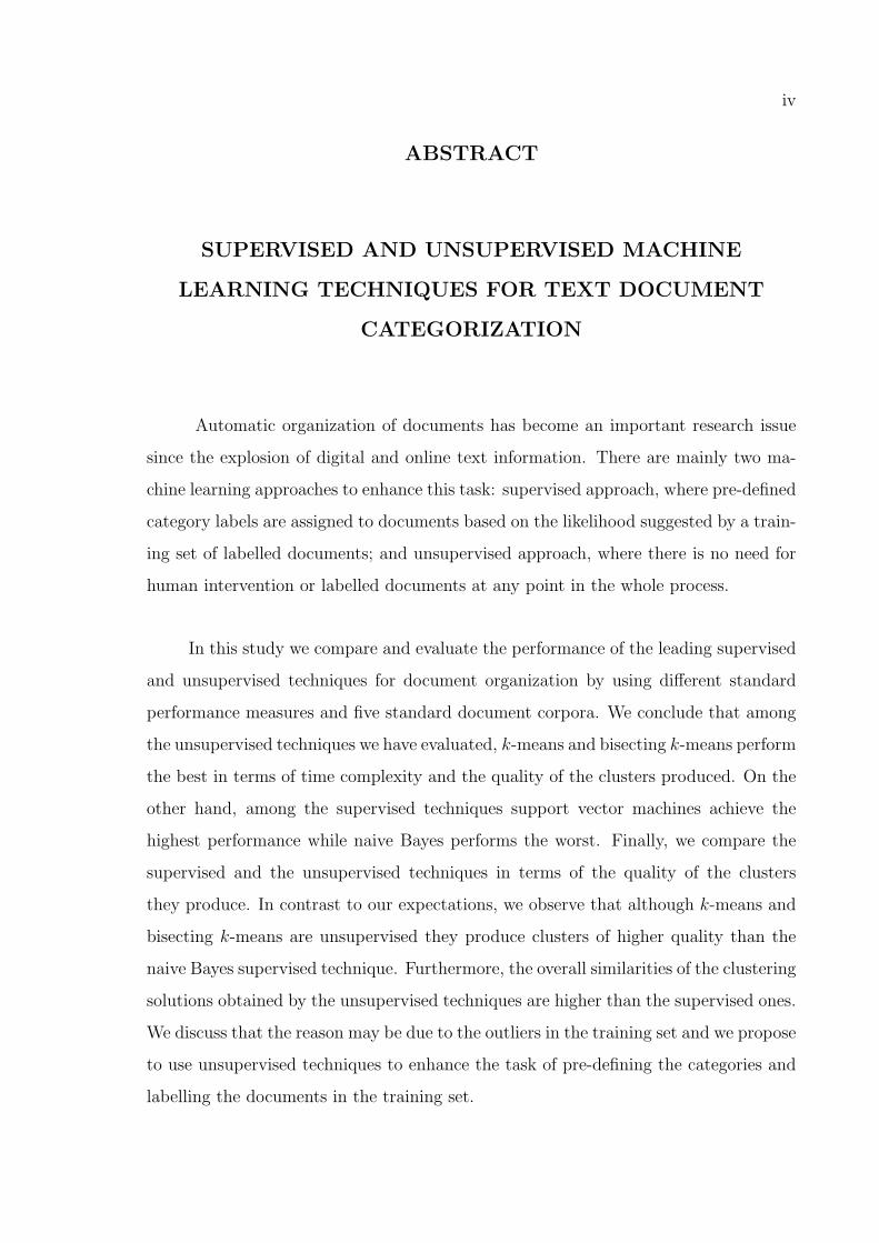
ABSTRACT

SUPERVISED AND UNSUPERVISED MACHINE

LEARNING TECHNIQUES FOR TEXT DOCUMENT

CATEGORIZATION

Automatic organization of documents has become an important research issue

since the explosion of digital and online text information. There are mainly two ma-

chine learning approaches to enhance this task: supervised approach, where pre-defined

category labels are assigned to documents based on the likelihood suggested by a train-

ing set of labelled documents; and unsupervised approach, where there is no need for

human intervention or labelled documents at any point in the whole process.

In this study we compare and evaluate the performance of the leading supervised

and unsupervised techniques for document organization by using different standard

performance measures and five standard document corpora. We conclude that among

the unsupervised techniques we have evaluated, k-means and bisecting k-means perform

the best in terms of time complexity and the quality of the clusters produced. On the

other hand, among the supervised techniques support vector machines achieve the

highest performance while naive Bayes performs the worst. Finally, we compare the

supervised and the unsupervised techniques in terms of the quality of the clusters

they produce. In contrast to our expectations, we observe that although k-means and

bisecting k-means are unsupervised they produce clusters of higher quality than the

naive Bayes supervised technique. Furthermore, the overall similarities of the clustering

solutions obtained by the unsupervised techniques are higher than the supervised ones.

We discuss that the reason may be due to the outliers in the training set and we propose

to use unsupervised techniques to enhance the task of pre-defining the categories and

labelling the documents in the training set.

v

OZET

BELGE SINIFLANDIRMA ICIN GOZETIMLI VE

GOZETIMSIZ OGRENME ALGORITMALARI

Bilgisayar ve elektronik teknolojilerinin gelismesi, Internet ve Web’in yaygınlas-

masıyla elektronik belgelerin miktarı her gecen gun artmaktadır. Bu elektronik veri-

tabanlarında ilgili verilere daha hızlı, kolay, ve dogru bir sekilde erisebilmek icin bel-

gelerin otomatik olarak sınıflandırılması onem kazanmıstır. Otomatik sınıflandırma icin

temelde iki yapay ogrenme yaklasımı vardır: gozetimli ogrenme ve gozetimsiz ogrenme.

Gozetimli ogrenmede, onceden sınıfların bilinmesi ve bu sınıflara ait belgelerden olusan

bir ogrenme kumesi gerekir. Gozetimsiz ogrenmede ise sınıfların onceden bilinmesine

ve herhangi bir asamada insan yardımına ihtiyac yoktur.

Bu calısmada otomatik belge sınıflandırma icin gozetimli ve gozetimsiz temel

yontemleri ele alıyoruz. Bu temel yontemlerin bes standart veritabanı uzerindeki

basarımlarını farklı kıstaslara dayanarak inceliyor, gozetimli ve gozetimsiz ogrenme

yaklasımlarını birbiriyle kıyaslıyoruz. Bu calısma sonucunda gozetimsiz yontemler

icinde k-means ve bisecting k-means’in belge obeklenmesi icin daha elverisli oldugunu

gorduk. Gozetimli yontemler arasında en iyi basarımı destek vektor makinaları elde

ediyor. Gozetimsiz yontemler olmalarına ragmen k-means ve bisecting k-means goze-

timli bir yontem olan naive Bayes’den daha kaliteli obekler olusturuyor. Gozetimsiz

yontemlerin olusturdugu obeklerin toplam benzerligi gozetimli yontemlerininkinden

genellikle daha yuksek. Bu sonuc ogrenme kumesinde hatalı bazı belgelerin olmasından

kaynaklanıyor olabilir. Bu nedenle sınıfların belirlenmesi ve ogrenme kumesinin olustu-

rulması asamasında gozetimsiz yontemlerden faydalanılmasını oneriyoruz.

vi

TABLE OF CONTENTS

ACKNOWLEDGEMENTS . . . . . . . . . . . . . . . . . . . . . . . . . . . . . iii

ABSTRACT . . . . . . . . . . . . . . . . . . . . . . . . . . . . . . . . . . . . . iv

OZET . . . . . . . . . . . . . . . . . . . . . . . . . . . . . . . . . . . . . . . . . v

LIST OF FIGURES . . . . . . . . . . . . . . . . . . . . . . . . . . . . . . . . . viii

LIST OF TABLES . . . . . . . . . . . . . . . . . . . . . . . . . . . . . . . . . . xiv

LIST OF SYMBOLS/ABBREVIATIONS . . . . . . . . . . . . . . . . . . . . . xvi

1. INTRODUCTION . . . . . . . . . . . . . . . . . . . . . . . . . . . . . . . . 1

1.1. Document Classification . . . . . . . . . . . . . . . . . . . . . . . . . . 1

1.2. Document Clustering . . . . . . . . . . . . . . . . . . . . . . . . . . . . 3

1.3. Motivation . . . . . . . . . . . . . . . . . . . . . . . . . . . . . . . . . . 4

1.4. Thesis Organization . . . . . . . . . . . . . . . . . . . . . . . . . . . . 5

2. DOCUMENT PREPROCESSING AND REPRESENTATION . . . . . . . . 7

2.1. Parsing the Documents and Case-folding . . . . . . . . . . . . . . . . . 8

2.2. Removing Stopwords . . . . . . . . . . . . . . . . . . . . . . . . . . . . 8

2.3. Stemming . . . . . . . . . . . . . . . . . . . . . . . . . . . . . . . . . . 9

2.4. Term Weighting . . . . . . . . . . . . . . . . . . . . . . . . . . . . . . . 11

2.4.1. Boolean Weighting . . . . . . . . . . . . . . . . . . . . . . . . . 11

2.4.2. Term Frequency Weighting . . . . . . . . . . . . . . . . . . . . . 12

2.4.3. Term Frequency × Inverse Document Frequency Weighting . . . 12

2.4.4. TF×IDF Weighting with Length Normalization . . . . . . . . . 13

2.5. Dimensionality Reduction . . . . . . . . . . . . . . . . . . . . . . . . . 13

2.5.1. Information Gain (IG) . . . . . . . . . . . . . . . . . . . . . . . 13

2.5.2. Mutual Information (MI) . . . . . . . . . . . . . . . . . . . . . . 14

2.5.3. Chi-Square Statistic . . . . . . . . . . . . . . . . . . . . . . . . 15

2.5.4. Term Strength (TS) . . . . . . . . . . . . . . . . . . . . . . . . 16

2.5.5. Document Frequency (DF) Thresholding . . . . . . . . . . . . . 17

2.6. Document Similarity Measure . . . . . . . . . . . . . . . . . . . . . . . 18

3. UNSUPERVISED TECHNIQUES FOR DOCUMENT CLUSTERING . . . 19

3.1. Partitional Clustering Techniques . . . . . . . . . . . . . . . . . . . . . 19

vii

3.1.1. K-Means Clustering . . . . . . . . . . . . . . . . . . . . . . . . 19

3.1.2. Bisecting K-Means . . . . . . . . . . . . . . . . . . . . . . . . . 20

3.2. Hierarchical Clustering Techniques . . . . . . . . . . . . . . . . . . . . 21

3.2.1. Divisive Hierarchical Clustering . . . . . . . . . . . . . . . . . . 21

3.2.2. Agglomerative Hierarchical Clustering . . . . . . . . . . . . . . 22

3.2.2.1. Single-link . . . . . . . . . . . . . . . . . . . . . . . . . 22

3.2.2.2. Complete-link . . . . . . . . . . . . . . . . . . . . . . . 23

3.2.2.3. Average-link . . . . . . . . . . . . . . . . . . . . . . . 23

4. SUPERVISED TECHNIQUES FOR DOCUMENT CLASSIFICATION . . . 24

4.1. K Nearest Neighbor Classification . . . . . . . . . . . . . . . . . . . . . 24

4.2. Naive Bayes Approach . . . . . . . . . . . . . . . . . . . . . . . . . . . 25

4.2.1. Multinomial Model . . . . . . . . . . . . . . . . . . . . . . . . . 26

4.2.2. Multivariate Bernoulli Model . . . . . . . . . . . . . . . . . . . 27

4.3. Support Vector Machines . . . . . . . . . . . . . . . . . . . . . . . . . . 28

5. EXPERIMENT RESULTS . . . . . . . . . . . . . . . . . . . . . . . . . . . . 30

5.1. Document Data Sets . . . . . . . . . . . . . . . . . . . . . . . . . . . . 30

5.2. Evaluation of the Clustering Techniques . . . . . . . . . . . . . . . . . 33

5.2.1. Evaluation Metrics . . . . . . . . . . . . . . . . . . . . . . . . . 33

5.2.1.1. Overall Similarity . . . . . . . . . . . . . . . . . . . . . 34

5.2.1.2. Purity . . . . . . . . . . . . . . . . . . . . . . . . . . . 34

5.2.1.3. Entropy . . . . . . . . . . . . . . . . . . . . . . . . . . 35

5.2.1.4. F-measure . . . . . . . . . . . . . . . . . . . . . . . . . 35

5.2.2. Results and Discussion . . . . . . . . . . . . . . . . . . . . . . . 36

5.3. Evaluation of the Classification Techniques . . . . . . . . . . . . . . . . 53

5.3.1. Evaluation Metrics . . . . . . . . . . . . . . . . . . . . . . . . . 53

5.3.1.1. Micro-averaged F1-measure . . . . . . . . . . . . . . . 55

5.3.1.2. Macro-averaged F1-measure . . . . . . . . . . . . . . . 55

5.3.2. Results and Discussion . . . . . . . . . . . . . . . . . . . . . . . 56

6. COMPARISON OF THE SUPERVISED AND UNSUPERVISED METHODS 62

7. CONCLUSIONS AND FUTURE WORK . . . . . . . . . . . . . . . . . . . . 66

APPENDIX A: STATISTICS OF THE CLUSTERING ALGORITHMS . . . . 70

REFERENCES . . . . . . . . . . . . . . . . . . . . . . . . . . . . . . . . . . . . 94

viii

LIST OF FIGURES

Figure 1.1. ML approaches used in this thesis for document categorization . . 6

Figure 2.1. Portion of the stopword list used . . . . . . . . . . . . . . . . . . . 9

Figure 2.2. Sample of words and their corresponding stems found by Porter’s

Stemming Algorithm . . . . . . . . . . . . . . . . . . . . . . . . . 10

Figure 3.1. Inter-cluster similarity defined by single-link, complete-link, and

average-link . . . . . . . . . . . . . . . . . . . . . . . . . . . . . . 22

Figure 4.1. Support vector machines find the hyperplane h that separates pos-

itive and negative training examples with maximum margin. Sup-

port vectors are marked with circles . . . . . . . . . . . . . . . . . 28

Figure 5.1. Class names of Reuters-21578 data set . . . . . . . . . . . . . . . . 32

Figure 5.2. Class names of the Wap data set . . . . . . . . . . . . . . . . . . . 33

Figure 5.3. Comparison of entropy, F-measure, purity, and overall similarity

values for online k-means, bisecting k-means, single-link, complete-

link, average-link and divisive clustering algorithms over Classic3

data set . . . . . . . . . . . . . . . . . . . . . . . . . . . . . . . . 40



link, average-link and divisive clustering algorithms over Wap data

set . . . . . . . . . . . . . . . . . . . . . . . . . . . . . . . . . . . 41

ix



link, average-link and divisive clustering algorithms over Reuters-

21578 data set . . . . . . . . . . . . . . . . . . . . . . . . . . . . . 42



link, average-link and divisive clustering algorithms over LA1 data

set . . . . . . . . . . . . . . . . . . . . . . . . . . . . . . . . . . . 43



link, average-link and divisive clustering algorithms over Hitech

data set . . . . . . . . . . . . . . . . . . . . . . . . . . . . . . . . 44

Figure 5.8. Term distributions of Classic3, Wap, Reuters-21578, LA1, and Hitech

data sets . . . . . . . . . . . . . . . . . . . . . . . . . . . . . . . . 45

Figure 5.9. Per cent of documents in Classic3, Wap, Reuters-21578, LA1, and

Hitech document collections whose nearest neighbor belongs to a

different class . . . . . . . . . . . . . . . . . . . . . . . . . . . . . 46

Figure 5.10. The performance, cluster-class distribution, and most descriptive

5 features of each cluster, of the clustering solution obtained by

k-means for Classic3 data set . . . . . . . . . . . . . . . . . . . . . 48



bisecting k-means for Classic3 data set . . . . . . . . . . . . . . . 49

x



divisive hierarchical clustering for Classic3 data set . . . . . . . . 50



average-link for Classic3 data set . . . . . . . . . . . . . . . . . . . 51



complete-link for Classic3 data set . . . . . . . . . . . . . . . . . . 52



single-link for Classic3 data set . . . . . . . . . . . . . . . . . . . . 53

Figure 5.16. Effect of the degree of the polynomial kernel of SVM to the F1-

measure scores . . . . . . . . . . . . . . . . . . . . . . . . . . . . . 59

Figure 5.17. Effect of the variance of the RBF kernel of SVM to the F1-measure

scores . . . . . . . . . . . . . . . . . . . . . . . . . . . . . . . . . . 60

Figure A.1. The performance, cluster-class distribution, and most descriptive 5

features of the clustering solution obtained by k-means for Hitech 70

Figure A.2. The performance, cluster-class distribution, and most descriptive


bisecting k-means for Hitech data set . . . . . . . . . . . . . . . . 71



divisive hierarchical clustering for Hitech data set . . . . . . . . . 72

xi



average-link for Hitech data set . . . . . . . . . . . . . . . . . . . 73



complete-link for Hitech data set . . . . . . . . . . . . . . . . . . . 74



single-link for Hitech data set . . . . . . . . . . . . . . . . . . . . 75



k-means for LA1 data set . . . . . . . . . . . . . . . . . . . . . . . 76



bisecting k-means for LA1 data set . . . . . . . . . . . . . . . . . 77



divisive hierarchical clustering for LA1 data set . . . . . . . . . . . 78



average-link for LA1 data set . . . . . . . . . . . . . . . . . . . . . 79



complete-link for LA1 data set . . . . . . . . . . . . . . . . . . . . 80

xii



single-link for LA1 data set . . . . . . . . . . . . . . . . . . . . . . 81



k-means for Reuters-21578 data set . . . . . . . . . . . . . . . . . 82



bisecting k-means for Reuters-21578 data set . . . . . . . . . . . . 83



divisive hierarchical clustering for Reuters-21578 data set . . . . . 84



average-link for Reuters-21578 data set . . . . . . . . . . . . . . . 85



complete-link for Reuters-21578 data set . . . . . . . . . . . . . . 86



single-link for Reuters-21578 data set . . . . . . . . . . . . . . . . 87



k-means for Wap data set . . . . . . . . . . . . . . . . . . . . . . . 88

xiii



bisecting k-means for Wap data set . . . . . . . . . . . . . . . . . 89



divisive hierarchical clustering for Wap data set . . . . . . . . . . 90



average-link for Wap data set . . . . . . . . . . . . . . . . . . . . . 91



complete-link for Wap data set . . . . . . . . . . . . . . . . . . . . 92



single-link for Wap data set . . . . . . . . . . . . . . . . . . . . . . 93

xiv

LIST OF TABLES

Table 5.1. Summary description of document sets . . . . . . . . . . . . . . . . 30

Table 5.2. Micro-averaged F1-measure results for SVM with polynomial kernel

of degrees 1, 2, 3, 4, 5, 6, and 7 . . . . . . . . . . . . . . . . . . . . 56

Table 5.3. Macro-averaged F1-measure results for SVM with polynomial kernel

of degrees 1, 2, 3, 4, 5, 6, and 7 . . . . . . . . . . . . . . . . . . . . 57

Table 5.4. Micro-averaged F1-measure results for SVM with RBF kernel with

γ = 0.2, 0.4, 0.6, 0.8, 1.0, 1.2, 1.4 . . . . . . . . . . . . . . . . . . . . 57

Table 5.5. Macro-averaged F1-measure results for SVM with RBF kernel with

γ = 0.2, 0.4, 0.6, 0.8, 1.0, 1.2, 1.4 . . . . . . . . . . . . . . . . . . . . 57

Table 5.6. Micro-averaged F1-measure results for the supervised techniques . 61

Table 5.7. Macro-averaged F1-measure results for the supervised techniques . 61

Table 6.1. Quality of the clusters (k=3) obtained by the unsupervised and the

supervised techniques for Classic3 . . . . . . . . . . . . . . . . . . 62


supervised techniques for Hitech . . . . . . . . . . . . . . . . . . . 63


supervised techniques for LA1 . . . . . . . . . . . . . . . . . . . . 63

Table 6.4. Quality of the clusters (k=90) obtained by the unsupervised and

the supervised techniques for Reuters-21578 . . . . . . . . . . . . . 64

xv

Table 6.5. Quality of the clusters (k=20) obtained by the unsupervised and

the supervised techniques for Wap . . . . . . . . . . . . . . . . . . 64

xvi

LIST OF SYMBOLS/ABBREVIATIONS

Act Number of documents that belong to category c and contain

term t

Bct Number of documents that do not belong to category c but

contain term t

Bit 1 if term t appears in document di, 0 otherwise

C Cluster

|C| Number of documents in cluster C

c Category

c Centroid vector

Cct Number of documents that belong to category c but do not

contain term t

Ci Cluster i

ci Category i

ci Feature vector of centroid i

Cj Cluster j

cj Category j

D Set of documents

d Degree of the polynomial kernel of the support vector ma-

chines

d A document vector

d′ A document vector

Dct Number of documents that do not belong to category c and

do not contain term t

di Document i

di Feature vector of document i

|di| Number of terms in document i

dj Document j

Ej Entropy of cluster j

f Target function

f ′ Classifier function

xvii

fij Observed frequency of the cell in row i and column j

fij Expected frequency of the cell in row i and column j

FNi The number of documents that are not assigned to category

i by the classifier but which actually belong to category i

FPi The number of documents that do not belong to category i

but are assigned to category i by the classifier incorrectly

Ij Internal cluster similarity of cluster j

k Requested number of clusters

M Number of categories

N Number of documents in the document corpus

Ni Number of documents in the corpus where term i appears

ni Size of cluster i

nij Number of documents with class label i in cluster j

Nj Number of documents in the corpus where term j appears

nj Size of cluster j

Pj Purity of cluster j

S Set of predefined categories

T Term space

|T | Number of terms in the document collection

t term

ti The ith term occurring in document di

tk The kth term occurring in document di

tfi Raw frequency of term i in the specified document

tfj Raw frequency of term j in the specified document

TPi The number of documents assigned correctly to category i

wi Weight of term i in document vector d

vt The tth term in the term space |T |x Test document vector

β Degree of importance in the range [0, +∞] given to π and ρ

in Fβ-Measure

χ2 Chi-square distribution

xviii

γ Variance of the RBF kernel of SVM

π Precision

πi Precision for category i

ρ Recall

ρi Recall for category i

DF Document Frequency

FN False Negatives

FP False Positives

HTML Hyper Text Markup Language

IDF Inverse Document Frequency

IG Information Gain

IR Information Retrieval

k-NN k-nearest neighbor

LLSF Linear Least Squares Fit

MI Mutual Information

ModApte Modified Apte

MPT Most Prevailing Topic, i.e, the topic that has the greatest

number of documents in the given cluster

NB Naive Bayes

NLP Natural Language Processing

NNet Neural Networks

RBF Radial Basis Function

SGML Standard Generalized Markup Language

SVM Support Vector Machines

TF Term Frequency

TP True Positives

TREC Text Retrieval Conference

TS Term Strength

WWW World Wide Web

1

1. INTRODUCTION

The amount of electronic text information available such as electronic publica-

tions, digital libraries, electronic books, email messages, news articles, and Web pages

is increasing rapidly. However, as the volume of online text information increases the

challenge of extracting relevant knowledge increases as well. The need for tools that

enhance people find, filter, and manage these resources has grown. Thus, automatic

organization of text document collections has become an important research issue. A

number of machine learning techniques have been proposed to enhance automatic or-

ganization of text data. These techniques can be grouped in two main categories as

supervised (document classification) and unsupervised (document clustering).

1.1. Document Classification

Text classification, also known as text categorization or topic spotting, is a super-

vised learning task, where pre-defined category labels are assigned to documents based

on the likelihood suggested by a training set of labelled documents. Until this machine

learning approach to text categorization, the most popular approach was knowledge

engineering. In knowledge engineering, expert knowledge is used to define manually

a set of rules on how to classify documents under the pre-defined categories. It is

discussed in [1] that the machine learning approach to document classification leads to

time and cost savings in terms of expert manpower without loss in accuracy. In the

problem of text classification we have a set D of documents and a set S of pre-defined

categories. The aim is to assign a boolean value to each 〈di, cj〉 pair, where di ∈ D

and cj ∈ S. A value of true assigned to 〈di, cj〉 stands for the decision of assigning

document di to category cj. Analogously, value of false assigned to 〈di, cj〉 stands

for the decision of not assigning document di to category cj. To state more formally,

the task is to approximate the unknown target function f : D × S → {true, false},that describes the way the documents should actually be classified, by the classifier

function f ′ : D × S → {true, false} such that number of decisions of f and f ′ that do

not coincide is minimized.

2

Many learning algorithms such as k-nearest neighbor (k-NN) [2, 3, 4], Support

Vector Machines (SVM) [5], neural networks (NNet) [6, 7], linear least squares fit

(LLSF) [8], and naive Bayes (NB) [9, 10] have been applied to text classification. A

comparison of these techniques is presented by Yang and Liu in [8]. They conclude

that all these techniques perform comparably when each category contains over 300

documents. However, when the number of positive training documents per category is

less than 10, SVM, k-NN, and LLSF outperform significantly NNet and NB.

Text categorization has many interesting application areas such as document

organization, text filtering and hierarchical categorization of Web pages. Document

organization is the task of structuring documents of a corporate document base into

folders, which may be hierarchical or flat. For instance, advertisements incoming to a

newspaper office may be classified into categories such as Cars, Real Estate, Computers,

and so on before publication. Similarly, Larkey has used document categorization

to organize patents into categories to enhance their search in [11]. Text filtering is

the process of classifying a dynamic collection of text documents into two disjoint

categories as relevant and irrelevant. An example is a newsfeed system where news

articles incoming to a newspaper from a news agency such as Reuters are filtered [1].

If it is a sports newspaper, delivery of news articles not related to sport are blocked.

Similarly, an email filter may be trained to classify incoming messages as spam or not

spam, and block the delivery of spam messages [12, 13]. Hierarchically categorizing

web pages or sites facilitates searching and browsing operations. Rather than posing

a generic query to a general purpose search engine, it is easier and more effective to

first navigate in the hierarchy of categories and restrict the search to the particular

categories of interest. To classify documents hierarchically, generally the classification

problem is subdivided into smaller classification problems. Hierarchical classification

of documents is addressed by Koller and Sahami in [10] and by Dumais and Chen in

[14].

3

1.2. Document Clustering

Unlike document classification, document clustering is an unsupervised learning

task, which does not require pre-defined categories and labelled documents. The aim

of text clustering is to group text documents such that intra-group similarities are high

and inter-group similarities are low. Document clustering has many application areas.

In Information Retrieval (IR), it has been used to improve precision and recall, and as

an efficient method to find similar documents. More recently, document clustering has

been used in automatically generating hierarchical groupings of documents by Koller

and Sahami in [10] and in document browsing to organize the results returned by a

search engine by Zamir et al. in [15].

Machine learning algorithms for clustering can be categorized into two main

groups as hierarchical clustering algorithms and partitional clustering algorithms [16].

Hierarchical algorithms produce nested partitions of data by splitting (divisive ap-

proach) or merging (agglomerative approach) clusters based on the similarity among

them. Divisive algorithms start with one cluster of all data points and at each itera-

tion split the most appropriate cluster until a stopping criterion such as a requested

number k of clusters is achieved. Conversely, in agglomerative algorithms each item

starts as an individual cluster and at each step, the most similar pair of clusters are

merged. Agglomerative hierarchical clustering algorithms can be further categorized

as single-link, complete-link, and average-link according to the way they define cluster

similarity. While agglomerative hierarchical clustering is a commonly used hierarchical

approach for document clustering, divisive approach has not been studied much as an

approach for document clustering. Evaluation of hierarchical clustering algorithms for

document data sets is presented by Zhao and Karypis in [17].

Partitional clustering algorithms group the data into un-nested non-overlapping

partitions that usually locally optimize a clustering criterion. Popular partitional clus-

tering techniques applied to the domain of text documents are k-means and its vari-

ant bisecting k-means. A comparison of agglomerative hierarchical techniques with

k-means and bisecting k-means is performed by Steinbach et al. in [18] and it has

4

been shown that average-link algorithm generally performs better than single-link and

complete-link algorithms for the document data sets used in the experiments. Next,

average-link algorithm is compared with k-means and bisecting k-means and it has

been concluded that bisecting k-means performs better than average-link agglomera-

tive hierarchical clustering algorithm and k-means in most cases for the data sets used

in the experiments.

1.3. Motivation

Various supervised machine learning techniques have been applied to document

classification. However, text classification requires the extra effort to predefine the

categories and to assign category labels to the documents in the training set. This

can be very tedious in large and dynamic text databases such as the WWW. An-

other phenomenon that poses a challenge to document categorization is inter-indexer

inconsistency discussed by Sebastiani in [1]. This phenomenon states that two human

experts may disagree when deciding under which category to categorize a given doc-

ument. For instance a news story about Bill Clinton and Monika Lewinsky may be

classified under the category Politics, or under the category Gossip, or under the both

categories, or under neither of the categories depending on the subjective judgement

of the human indexer [1].

The dynamic nature of most text databases makes it challenging to pre-define

the categories and the subjectivity in assigning documents to categories has lead us to

believe that by nature text organization should be an unsupervised task rather than a

supervised one. Therefore, we concentrated on text clustering which is an unsupervised

task where no human intervention at any point in the whole process and no labelled

documents are provided. There are many challenges in using the existing machine

learning techniques in the domain of text documents. We can list them as follows:

• Number of documents to be clustered is usually very large.

• The feature space is usually very large.

• It is usually very difficult to determine the number of clusters in advance.

5

• Some documents may belong to more than one cluster (overlapping clusters).

• Shape of clusters may be arbitrary.

• The process should be online considering the dynamic structure of text databases

such as the WWW.

Our aim in this study is to compare and evaluate the performance of the com-

monly used supervised and unsupervised techniques for text document organization.

We propose that unsupervised techniques can be used to give feedback to the human

indexers to enhance the task of pre-defining categories and preparing a labelled train-

ing set. This study will form the basis for developing a hybrid approach of supervised

and unsupervised paradigm to the domain of text documents by also considering the

challenges stated above.

1.4. Thesis Organization

The outline of this thesis is as follows. In Chapter 2 we discuss how we preprocess

and represent documents so that machine learning algorithms can be applied to them.

We overview the unsupervised clustering algorithms and the supervised classification

algorithms that we evaluate in Chapter 3 and Chapter 4 respectively. Figure 1.1

displays the taxonomy of the ML techniques, that we evaluated for document clustering

and classification in this study. In Chapter 5 we describe the standard document data

sets we have used in the experiments, our experimental methodology, evaluation metrics

and the results we have obtained. In Chapter 6 we perform a comparative study of

the supervised techniques with the unsupervised ones. We conclude and outline future

directions of research in Chapter 7.

6

M L Approaches for Document Categorization

UnsupervisedApproach(Clustering)

SupervisedApproach

(Classification)

PartitionalClustering

HierarchicalClustering

Divisive

Agglomerative

Single-link

Completelink

Average-link

K-NN Naive Bayes SVM

K-means

Bisectingk-means

Traditional

W eighted

Polynomialkernel

RBF Kernel

Figure 1.1. ML approaches used in this thesis for document categorization

7

2. DOCUMENT PREPROCESSING AND

REPRESENTATION

In order to cluster or classify text documents by applying machine learning tech-

niques, documents should first be preprocessed. In the preprocessing step, the docu-

ments should be transformed into a representation suitable for applying the learning

algorithms. The most widely used method for document representation is the vector-

space model introduced by Salton et al. [19], which we have also decided to employ. In

this model, each document is represented as a vector d. Each dimension in the vector

d stands for a distinct term in the term space of the document collection.

A term in the document collection can stand for a distinct single-word, a stemmed

word or a phrase. Phrases consist of multiple words such as “data mining” or “mobile

phone” and constitute a different context than when used separately. Phrases can be

extracted by using statistical or Natural Language Processing (NLP) techniques. By

statistical methods phrases can be extracted by considering the frequently appearing

sequences of words in the document collection [20]. A research on extracting phrases

by using NLP techniques for text categorization is discussed by Fuernkranz et al. [21].

Phrases can also be extracted by manually defining the phrases for a particular domain

such as done to filter spam mail in [13]. However, this does not fulfill our requirement

to organize documents in generic domains such as the Web.

In vector space representation, defining terms as distinct single words is referred

to as “bag of words” representation. Some researchers state that using phrases rather

than single words to define terms produce more accurate classification results [20, 21];

whereas others argue that using single words as terms does not produce worse results

[22, 23]. As “bag of words” representation is the most frequently used method for

defining terms and it is computationally more efficient than the phrase representation,

we have chosen to adapt this method to define terms of the feature space.

8

One challenge emerging when terms are defined as single words is that the feature

space becomes very high dimensional. In addition, words which are in the same context

such as biology and biologist are defined as different terms. So, in order to define

words that are in the same context with the same term and consequently to reduce

dimensionality we have decided to define the terms as stemmed words. To stem the

words, we have chosen to use Porter’s Stemming Algorithm [24], which is the most

commonly used algorithm for word stemming in English.

Preprocessing and document representation phase, which is implemented in Mi-

crosoft Visual C++ 6.0, consists of the following steps:

• Parsing the documents and case-folding

• Removing stopwords

• Stemming

• Term weighting

• Dimensionality reduction

These steps will be described briefly in the following sections.

2.1. Parsing the Documents and Case-folding

In this step, all the HTML or SGML mark-up tags and non-alpha characters are

removed from the documents in the document corpora. Case-folding, which stands

for converting all the characters in a document into the same case, is performed by

converting all the characters into lower-case. Tokens consisting of alpha characters are

extracted.

2.2. Removing Stopwords

There are words in English such as pronouns, prepositions and conjunctions that

are used to provide structure in the language rather than content. These words, which

are encountered very frequently and carry no useful information about the content and

9

a alone anyways b between

a’s along anywhere be beyond

able already apart became both

about also appear because brief

above although appreciate become but

according always appropriate becomes by

accordingly am are becoming c

across among aren’t been c’mon

actually amongst around before c’s

after an as beforehand came

afterwards and aside behind can

again another ask being can’t

against any asking believe cannot

ain’t anybody associated below cant

all anyhow at beside cause

allow anyone available besides causes

allows anything away best certain

almost anyway awfully better certainly

Figure 2.1. Portion of the stopword list used

thus the category of documents, are called stopwords. Removing stopwords from the

documents is very common in information retrieval. We have decided to eliminate the

stopwords from the documents, which will lead to a drastic reduction in the dimen-

sionality of the feature space. The list of 571 stopwords used in the Smart system is

used [19]. This stopword list is obtained from [25]. Figure 2.1 shows a portion of the

stopword list.

2.3. Stemming

In order to define words that are in the same context with the same term and

consequently to reduce dimensionality, we have decided to define the terms as stemmed

words. To stem the words, we have chosen to use Porter’s Stemming Algorithm [24],

10

Word: ponies Stem: poni

Word: caress Stem: caress

Word: cats Stem: cat

Word: feed Stem: fe

Word: agreed Stem: agre

Word: plastered Stem: plaster

Word: motoring Stem: motor

Word: sing Stem: sing

Word: conflated Stem: conflat

Word: troubling Stem: troubl

Word: sized Stem: size

Word: hopping Stem: hop

Word: tanned Stem: tan

Word: falling Stem: fall

Word: fizzed Stem: fizz

Word: failing Stem: fail

Word: filing Stem: file

Word: happy Stem: happi

Figure 2.2. Sample of words and their corresponding stems found by Porter’s

Stemming Algorithm

which is the most commonly used algorithm for word stemming in English. In this way

for instance, we reduce the similar terms “ computer”, “ computers”, and “ computing”

to the word stem “ comput”. Implementation of Porter’s Stemming Algorithm in C is

downloaded from [26]. This algorithm is embedded to the preprocessing system. Figure

2.2 displays a sample of words and the stems produced by Porter’s Stemming Algo-

rithm. After stemming, terms that are shorter than two characters are also removed

as they do not carry much information about the content of a document.

11

2.4. Term Weighting

We represent each document vector d as

d = (w1, w2, ..., w|T |) (2.1)

where wi is the weight of ith term of document d and |T | is the number of distinct

terms in the document collection. There are various term weighting approaches most

of which are based on the following observations [27]:

• The relevance of a word to the topic of a document is proportional to the number

of times it appears in the document.

• The discriminating power of a word between documents is less, if it appears in

most of the documents in the document collection.

A comparative study of different term weighting approaches in automatic text retrieval

is presented by Salton and Buckley in [28]. The term weighting approach we have

applied and some other standard term weighting functions are discussed in the following

subsections. We define:

tfi as the raw frequency of term i in document d;

N as the total number of documents in the document corpus;

Ni as the number of documents in the corpus where term i appears; and

|T | as the number of distinct terms in the document collection (after stopword removal

and stemming is performed).

2.4.1. Boolean Weighting

Boolean weighting is the simplest method for term weighting. In this approach,

the weight of a term is assigned to be 1 if the term appears in the document and it is

12

assigned to be 0 if the term does not appear in the document.

wi =

⎧⎪⎨⎪⎩

1 if tfi > 0

0 otherwise(2.2)

2.4.2. Term Frequency Weighting

Term Frequency (TF) weighting is also a simple method for term weighting.

wi = tfi (2.3)

In this method, the weight of a term in a document is equal to the number of times the

term appears in the document, i.e. to the raw frequency of the term in the document.

2.4.3. Term Frequency × Inverse Document Frequency Weighting

Boolean weighting and TF weighting do not consider the frequency of the term

throughout all the documents in the document corpus. Term Frequency × Inverse

Document Frequency (TF×IDF) weighting is the most common method used for term

weighting that takes into account this property. In this approach, the weight of term i

in document d is assigned proportionally to the number of times the term appears in

the document, and in inverse proportion to the number of documents in the corpus in

which the term appears.

wi = tfi · log(

N

Ni

)(2.4)

TF×IDF weighting approach weights the frequency of a term in a document with a

factor that discounts its importance if it appears in most of the documents, as in this

case the term is assumed to have little discriminating power.

13

2.4.4. TF×IDF Weighting with Length Normalization

In this approach, to account for documents of different lengths each document

vector is normalized so that it is of unit length.

wi =tfi · log

(NNi

)√∑|T |

j=1

[tfj · log

(NNj

) ]2(2.5)

Salton and Buckley discuss that TF×IDF weighting with length normalization

generally performs better than the other techniques [28]. Therefore, we applied this

weighting approach in our study.

2.5. Dimensionality Reduction

There are various methods applied for dimensionality reduction in document cat-

egorization. Some common examples are Information Gain (IG), Mutual Informa-

tion (MI), Chi-Square Statistic, Term Strength (TS), and Document Frequency (DF)

Thresholding. We discuss these techniques briefly in the following subsections.

2.5.1. Information Gain (IG)

Information gain measures the number of bits of information gained for category

prediction when the presence or absence of a term in a document is known. When the

set of possible categories is {c1, c2, ..., cm}, the IG for each unique term t is calculated

as follows [4]:

IG(t) = −m∑

i=1

P (ci)·log P (ci)+P (t)·m∑

i=1

P (ci|t)·log P (ci|t)+P (t)·m∑

i=1

P (ci|t)·log P (ci|t)(2.6)

As seen from Equation 2.5, IG calculates the decrease in entropy when the feature is

given vs. absent. P (ci) is the prior probability of category ci. It can be estimated

from the fraction of documents in the training set belonging to category ci. P (t) is

14

the prior probability of term t. It can be estimated from the fraction of documents in

the training set in which term t is present. Likewise, P (t) can be estimated from the

fraction of documents in the training set in which term t is absent. Terms whose IGs

are less than some predetermined threshold are removed from the feature space.

2.5.2. Mutual Information (MI)

Mutual information is a technique frequently used in statistical language mod-

elling of word associations and related applications [29]. MI between term t and

category c is defined to be [4]:

MI(t, c) = logP (t ∧ c)

P (t) × P (c)(2.7)

It is estimated by using [4]:

MI(t, c) ≈ logAct × N

(Act + Cct) × (Act + Bct)(2.8)

Here, Act is the number of times t and c co-occur, Bct is the number of times t occurs

without c, Cct is the number of times c occurs without t, and N is the total number of

documents. When t and c are independent MI(t, c) is equal to zero.

We can write equation 2.7 in the following equivalent form:

MI(t, c) = log P (t|c) − log P (t) (2.9)

It is seen from equation 2.9 that, for terms that have an equal conditional probability,

rare terms will have a higher MI value than common terms. So, MI technique has the

drawback that MI values are not comparable among terms with large frequency gaps.

Category specific MI scores for a term t can be combined into a global MI score

15

for that term in the following two ways[4]:

MIavg(t) =m∑

i=1

P (ci) × MI(t, ci) (2.10)

or

MImax(t) =m

maxi=1

{MI(t, ci)} (2.11)

Terms that have lower MI values than a predetermined threshold are eliminated.

2.5.3. Chi-Square Statistic

Chi-square (χ2) statistic is a measure of association. In statistics chi-square

measure is formulated as:

χ2 =∑

i

∑j

(fij − fij)2

fij

(2.12)

Here, fij is the observed frequency of the cell in row i and column j and fij is the

expected frequency of that cell. A more detailed discussion of the χ2 statistic can be

found in [30].

The χ2 statistic measures the degree of dependence between a certain term and

a certain category. That is, it measures to what degree a certain term is indicative

of membership or non-membership of a document in a certain category [31]. The χ2

statistic is reformulated and used for the task of document categorization by Yang and

Pedersen [4], Ng et al. [6], and Spitters [31] as follows:

χ2(t, c) =N × (ActDct − CctBct)

2

(Act + Cct) × (Bct + Dct) × (Act + Bct) × (Cct + Dct)(2.13)

Here, we have a 2 × 2 contingency table. The first row stands for the number of

documents that contain term t, the second row stands for the number of documents

16

that do not contain term t, the first column stands for the number of documents that

belong to category c, and the second column stands for the number of documents that

do not belong to category c. So, Act is the number of documents that belong to category

c and contain term t, Bct is the number of documents that do not belong to category

c but contain term t, Cct is the number of documents that belong to category c but

do not contain term t, Dct is the number of documents that do not belong to category

c and do not contain term t, and N is the total number of documents in the corpus.

Two different measures can be computed based on the χ2 statistic [4]:

χ2avg(t) =

m∑i=1

P (ci) × χ2(t, ci) (2.14)

or

χ2max(t) =

mmaxi=1

{χ2(t, ci)} (2.15)

Terms that have lower χ2 values than a predetermined threshold are eliminated.

2.5.4. Term Strength (TS)

Term strength method, estimates term importance based on how commonly a

term is likely to appear in closely related documents [4]. The first step in this method

is to use a training set of documents to find document pairs which have a similarity

larger than a predetermined threshold. In the next step TS is calculated based on the

estimated conditional probability that a term appears in the second document given

that it appears in the first one. Suppose, di and dj are any pair of distinct but related

documents. Then the TS of term t is defined to be [4]:

TS(t) = P (t ∈ dj|t ∈ di) (2.16)

Unlike IG, MI, and χ2 statistic, TS is an unsupervised dimensionality reduction tech-

nique where document categories are not used. It is based on document clustering and

assumes that documents with many shared words are related and the terms that are

17

heavily shared among these related documents are relatively informative.

2.5.5. Document Frequency (DF) Thresholding

Document frequency (DF ) of a term is the number of documents that term

appears. In this technique, the document frequency of each unique term is computed

and terms whose document frequencies are less than a predetermined threshold are

eliminated. The basic assumption behind this technique is that rare terms are either

non-informative for document categorization or they do not have much weight in global

performance. This technique can also lead to improvement in categorization accuracy

in case rare terms are noise terms. However, DF is usually not used for aggressive

term elimination because there is another widely accepted assumption in information

retrieval that low-DF terms are distinctive and thus relatively informative and for this

reason should not be removed aggressively [4].

A comparative study of feature selection in text categorization is presented by

Yang and Pedersen in [4]. It has been reported that IG and χ2 statistic performed the

best. However, DF , the simplest and the most efficient method in terms of compu-

tational complexity, performed similar to IG and χ2 statistics. It has been suggested

that DF can be reliably used instead of IG and χ2 statistics when computation per-

formances of the latter two are too expensive.

Another point to consider is that IG, MI and χ2 statistics are supervised tech-

niques and use information about term-category associations. As our main focus is

on unsupervised techniques for document organization, these methods are not suitable

to be applied in our study. To reduce the dimensionality of the data, we apply DF

Thresholding. We define the DF threshold as 1 and hence remove the terms that

appear in only one document.

18

2.6. Document Similarity Measure

To use a clustering or classification algorithm, a similarity measure between two

documents must be defined. In our study we use the widely used cosine similarity

measure to calculate the similarity of two documents. This measure is defined as [18]:

cos(d1,d2) =d1 • d2

‖d1‖‖d2‖ (2.17)

that is, it is the dot product of d1 and d2 divided by the lengths of d1 and d2.

19

3. UNSUPERVISED TECHNIQUES FOR DOCUMENT

CLUSTERING

In unsupervised clustering, we have unlabelled collection of documents. The aim

is to cluster the documents without additional knowledge or intervention such that

documents within a cluster are more similar than documents between clusters. Tradi-

tional clustering techniques can be categorized into two major groups as partitional and

hierarchical. In this chapter we discuss these groups and their main representatives.

3.1. Partitional Clustering Techniques

Partitional algorithms produce un-nested, non-overlapping partitions of docu-

ments that usually locally optimize a clustering criterion. The general methodology

is as follows: given the number of clusters k, an initial partition is constructed; next

the clustering solution is refined iteratively by moving documents from one cluster to

another. In the following sub-sections we discuss the most popular partitional algo-

rithm k-means, and its variant bisecting k-means which has been applied to cluster

documents by Steinbach et al. in [18] and has been shown to generally outperform

agglomerative hierarchical algorithms.

3.1.1. K-Means Clustering

The idea behind the k-means algorithm, discussed by Hartigan [32], is that each

of k clusters can be represented by the mean of the documents assigned to that cluster,

which is called the centroid of that cluster. It is discussed by Berkhin in [33] that there

are two versions of k-means algorithm known. The first version is the batch version

and is also known as Forgy’s algorithm [34]. It consists of the following two-step major

iterations:

(i) Reassign all the documents to their nearest centroids

20

(ii) Recompute centroids of newly assembled groups

Before the iterations start, firstly k documents are selected as the initial centroids.

Iterations continue until a stopping criterion such as no reassignments occur is achieved.

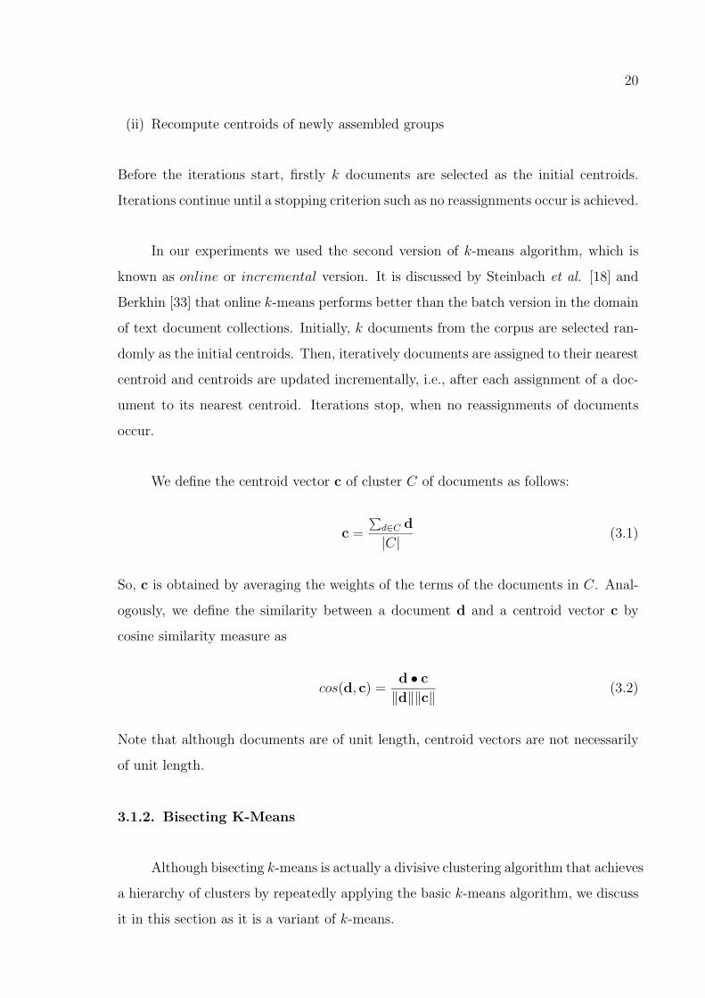
In our experiments we used the second version of k-means algorithm, which is

known as online or incremental version. It is discussed by Steinbach et al. [18] and

Berkhin [33] that online k-means performs better than the batch version in the domain

of text document collections. Initially, k documents from the corpus are selected ran-

domly as the initial centroids. Then, iteratively documents are assigned to their nearest

centroid and centroids are updated incrementally, i.e., after each assignment of a doc-

ument to its nearest centroid. Iterations stop, when no reassignments of documents

occur.

We define the centroid vector c of cluster C of documents as follows:

c =

∑d∈C d

|C| (3.1)

So, c is obtained by averaging the weights of the terms of the documents in C. Anal-

ogously, we define the similarity between a document d and a centroid vector c by

cosine similarity measure as

cos(d, c) =d • c

‖d‖‖c‖ (3.2)

Note that although documents are of unit length, centroid vectors are not necessarily

of unit length.

3.1.2. Bisecting K-Means

Although bisecting k-means is actually a divisive clustering algorithm that achieves

a hierarchy of clusters by repeatedly applying the basic k-means algorithm, we discuss

it in this section as it is a variant of k-means.

21

In each step of bisecting k-means a cluster is selected to be split and it is split

into two by applying basic k-means for k = 2. The largest cluster, that is the cluster

containing the maximum number of documents, or the cluster with the least overall

similarity can be chosen to be split. We performed experiments in both ways and

observed that they perform similarly. So, in the experiment results section we reveal

only the results of the case when the largest cluster is selected to be split.

3.2. Hierarchical Clustering Techniques

Hierarchical clustering algorithms produce a cluster hierarchy named a dendro-

gram [33]. These algorithms can be categorized as divisive (top-down) and agglomer-

ative (bottom-up) [16, 33]. We discuss these approaches in the following sub-sections.

3.2.1. Divisive Hierarchical Clustering

Divisive algorithms start with one cluster of all documents and at each iteration

split the most appropriate cluster until a stopping criterion such as a requested number

k of clusters is achieved.

A method to implement a divisive hierarchical algorithm is described by Kaufman

and Rousseeuw in [35]. In this technique in each step the cluster with the largest

diameter is split, i.e. the cluster containing the most distant pair of documents. As we

use document similarity instead of distance as a proximity measure, the cluster to be

split is the one containing the least similar pair of documents. Within this cluster the

document with the least average similarity to the other documents is removed to form

a new singleton cluster. The algorithm proceeds by iteratively assigning the documents

in the cluster being split to the new cluster if they have greater average similarity to

the documents in the new cluster. To our knowledge, divisive hierarchical clustering

in this sense has not been applied to document corpora. This method is not robust to

outliers and in our experiments we observe that documents in the cluster being split

generally tend to remain in the larger old cluster and for small number of clusters k,

clustering quality is not comparable with the other algorithms we evaluated. So, we

22

made a slight modification to this algorithm. In our version we select the least similar

pair of documents in the cluster being split and remove them to form two new singleton

clusters. The rest of the documents in the cluster are assigned iteratively to one of the

new clusters by taking the average similarity as criterion.

3.2.2. Agglomerative Hierarchical Clustering

Agglomerative clustering algorithms start with each document in a separate clus-

ter and at each iteration merge the most similar clusters until the stopping criterion

is met. They are mainly categorized as single-link, complete-link and average-link de-

pending on the method they define inter-cluster similarity. Figure 3.1 illustrates the

idea:

0

1

2

3

4

5

6

7

8

9

10

0 1 2 3 4 5 6 7 8 9 10

single-link

max. cos(di,dj)

0 1 2 3 4 5 6 7 8 9

complete-link

min. cos(di,dj)

0 1 2 3 4 5 6 7 8 9

average-link

average pairwise cos(di,dj)

Figure 3.1. Inter-cluster similarity defined by single-link, complete-link, and

average-link

3.2.2.1. Single-link. The single-link method defines the similarity of two clusters Ci

and Cj as the similarity of the two most similar documents di ∈ Ci and dj ∈ Cj:

similaritysingle−link(Ci, Cj) = maxdi∈Ci,dj∈Cj

|cos(di,dj)| (3.3)

23

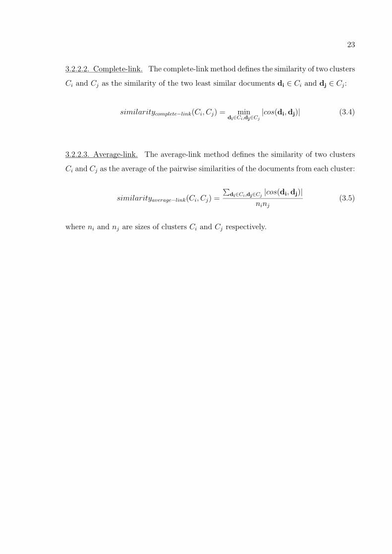
3.2.2.2. Complete-link. The complete-link method defines the similarity of two clusters

Ci and Cj as the similarity of the two least similar documents di ∈ Ci and dj ∈ Cj:

similaritycomplete−link(Ci, Cj) = mindi∈Ci,dj∈Cj

|cos(di,dj)| (3.4)

3.2.2.3. Average-link. The average-link method defines the similarity of two clusters

Ci and Cj as the average of the pairwise similarities of the documents from each cluster:

similarityaverage−link(Ci, Cj) =

∑di∈Ci,dj∈Cj

|cos(di,dj)|ninj

(3.5)

where ni and nj are sizes of clusters Ci and Cj respectively.

24

4. SUPERVISED TECHNIQUES FOR DOCUMENT

CLASSIFICATION

Supervised algorithms assume that the category structure or hierarchy of a text

database is already known. They require a training set of labelled documents and return

a function that maps documents to the pre-defined class labels. As discussed previously,

knowing the category structure in advance and generation of correctly labelled training

set are very challenging or even impossible in large and dynamic text databases. In

this section we discuss the most popular supervised algorithms k-NN, naive Bayes, and

support vector machines, that we have evaluated.

4.1. K Nearest Neighbor Classification

K-NN (k-nearest neighbor) classification is a popular instance-based learning

method [36] that has been shown to be a strong performer in the task of text catego-

rization [3, 8].

The algorithm works as follows: First, given a test document x, the k near-

est neighbors among the training documents are found. The category labels of these

neighbors are used to estimate the category of the test document. In the traditional

approach, the most common category label among the k-nearest neighbors is assigned

to the test document.

Weighted k-NN is a refinement to the traditional approach. In weighted k-NN, the

contribution of each of the k nearest neighbors is weighted according to its similarity to

the test document x. Then, for each category, the similarity of the neighbors belonging

to that category are summed to obtain the score of the category for x. That is, the

score of category cj for the test document x is

score(cj,x) =∑

di∈N(x)

cos(x,di) · y(di, cj) (4.1)

25

where di is a training document; N(x) is the set of the k training documents nearest

to x; cos(x,di) is the cosine similarity between the test document x and the training

document di; and y(di, cj) is a function whose value is 1 if di belongs to category cj

and 0 otherwise. The test document x is assigned to the category with the highest

score.

In our study, we evaluated both the traditional k-NN and weighted k-NN for

varying k parameter values and report the results of both approaches for the best k

value in the experiment results chapter.

4.2. Naive Bayes Approach

The naive Bayes (NB) classifier is a probabilistic model that uses the joint prob-

abilities of terms and categories to estimate the probabilities of categories given a test

document [36]. The naive part of the classifier comes from the simplifying assumption

that all terms are conditionally independent of each other given a category. Because of

this independence assumption, the parameters for each term can be learned separately

and this simplifies and speeds the computation operations compared to non-naive Bayes

classifiers.

There are two common event models for NB text classification, discussed by

McCallum and Nigam in [9], multinomial model and multivariate Bernoulli model. In

both models classification of test documents is performed by applying the Bayes’ rule

[36]:

P (cj|di) =P (cj) · P (di|cj)

P (di)(4.2)

where di is a test document and cj is a category. The posterior probability of each

category cj given the test document di, i.e. P (cj|di), is calculated and the category

with the highest probability is assigned to di. In order to calculate P (cj|di), P (cj) and

P (di|cj) have to be estimated from the training set of documents. Note that P (di)

is same for each category so we can eliminate it from the computation. The category

26

prior probability, P (cj), can be estimated as follows:

P (cj) =

∑Ni=1 y(di, cj)

N, (4.3)

where, N is number of training documents and y(di, cj) is defined as follows:

y(di, cj) =

⎧⎪⎨⎪⎩

1 if di ∈ cj

0 otherwise(4.4)

So, prior probability of category cj is estimated by the fraction of documents in the

training set belonging to cj. P (di|cj) parameters are estimated in different ways by

the multinomial model and multivariate Bernoulli model. We present these models in

the following two sub-sections.

4.2.1. Multinomial Model

In the multinomial model a document di is an ordered sequence of term events,

drawn from the term space T . The naive Bayes assumption is that the probability of

each term event is independent of term’s context, position in the document, and length

of the document. So, each document di is drawn from a multinomial distribution of

terms with number of independent trials equal to the length of di. The probability of

a document di given its category cj can be approximated as:

P (di|cj) ≈|di|∏i=1

P (ti|cj), (4.5)

where |di| is the number of terms in document di; and ti is the ith term occurring in

document di. Thus the estimation of P (di|cj) is reduced to estimating each P (ti|cj)

independently. The following Bayesian estimate is used for P (ti|cj):

P (ti|cj) =1 + TF (ti, cj)

|T | + ∑tk∈T TF (tk, cj)

(4.6)

27

Here, TF (ti, cj) is the total number of times term ti occurs in the training set documents

belonging to category cj. The summation term in the denominator stands for the total

number of term occurrences in the training set documents belonging to category cj.

This estimator is called Laplace estimator and assumes that the observation of each

word is a priori likely [37].

4.2.2. Multivariate Bernoulli Model

Multivariate Bernoulli model for naive Bayes classification is the event model we

used and evaluated in our study. In this model a document is represented by a vector of

binary features indicating the terms that occur and that do not occur in the document.

Here, the document is the event and absence or presence of terms are the attributes

of the event. The naive Bayes assumption is that the probability of each term being

present in a document is independent of the presence of other terms in a document.

To state differently, the absence or presence of each term is dependent only on the

category of the document. Then, P (di|cj), the probability of a document given its

category is simply the product of the probability of the attribute values over all term

attributes:

P (di|cj) =|T |∏t=1

(Bit · P (vt|cj) + (1 − Bit)(1 − P (vt|cj))), (4.7)

where |T | is the number of terms in the training set and Bit is defined as follows:

Bit =

⎧⎪⎨⎪⎩

1 if term t appears in document di

0 otherwise(4.8)

Thus, a document can be seen as a collection of multiple independent Bernoulli exper-

iments, one for each term in the term space. The probabilities of each of these term

events are defined by the class-conditional term probabilities P (vt|cj). We can estimate

the probability of term vt in category cj as follows:

P (vt|cj) =1 +

∑Ni=1 Bit · y(di, cj)

2 +∑N

i=1 y(di, cj), (4.9)

28

where, N is number of training documents and y(di, cj) is defined as in equation 4.4.

Different from the multinomial model, the multivariate Bernoulli model does

not take into account the number of times each term occurs in the document, and

it explicitly includes the non-occurrence probability of terms that are absent in the

document [9].

4.3. Support Vector Machines

Support Vector Machines (SVM) is a technique introduced by Vapnik in 1995,

which is based on the Structural Risk Minimization principle [38]. It is designed for

solving two-class pattern recognition problems. The problem is to find the decision

surface that separates the positive and negative training examples of a category with

maximum margin. Figure 4.1 illustrates the idea for linearly separable data points. A

decision surface in a linearly separable space is a hyperplane. The dashed lines parallel

to the solid line show how much the decision surface can be moved without leading

to a misclassification of data. Margin is the distance between these parallel lines.

Examples closest to the decision surface are called support vectors.

Figure 4.1. Support vector machines find the hyperplane h that separates positive

and negative training examples with maximum margin. Support vectors are marked

with circles

29

For the linearly separable case, the decision surface is a hyperplane that can be written

as [8]:

w • d + b = 0 (4.10)

where d is a document to be classified, and vector w and constant b are learned from the

training set. The SVM problem is to find w and b that satisfy the following constraints

[5]:

Minimize ||w||2 (4.11)

so that ∀i : yi[w • d + b] ≥ 1 (4.12)

Here, i ∈ {1, 2, ..., N}, where N is the number of documents in the training set; and

yi equals +1 if document di is a positive example for the category being considered

and equals −1 otherwise. This optimization problem can be solved by using quadratic

programming techniques [39].

SVM can be also used to learn non-linear decision functions such as polynomial

of degree d or radial basis function (RBF) with variance γ. These kernel functions can

be illustrated as follows:

Kpolynomial(d1,d2) = (d1 • d2 + 1)d (4.13)

Krbf (d1,d2) = exp(γ(d1 − d2)2) (4.14)

In our study we evaluated SVM with linear kernel, polynomial kernel with different

degrees, and with RBF kernel with different γ parameters. For our experiments we

used the SV M light system implemented by Joachims [40].

30

5. EXPERIMENT RESULTS

We experimentally evaluated the performance of the partitional and hierarchical

clustering techniques, and the supervised classification techniques for document orga-

nization on five different standard data sets. In this chapter we first describe the data

sets we used in our experiments and our experimental methodology. Next we present

and evaluate the experimental results for the unsupervised and supervised techniques

separately.

5.1. Document Data Sets

In our experiments we used five standard document corpora widely used in au-

tomatic text organization research. Summary description of these document sets after

preprocessing as described in Chapter 2 is presented in Table 5.1.

Table 5.1. Summary description of document sets

Data set # of documents # of classes # of terms

Classic3 3,891 3 6,729

Hitech 1,530 6 10,919

LA1 2,134 6 14,363

Reuters-21578 12,902 90 12,772

Wap 1,560 20 8,061

Classic3 data set contains 1,398 CRANFIELD documents from aeronautical sys-

tem papers, 1,033 MEDLINE documents from medical journals and 1,460 CISI docu-

ments from information retrieval papers.

The Hitech data set was derived from the San Jose Mercury newspaper articles

which are delivered as part of the TREC collection [41]. The classes of this document

corpora are computers, electronics, health, medical, research, and technology.

31

LA1 data set consists of documents from Los Angeles Times newspaper used in

TREC-5 [41]. The categories correspond to the desk of the paper that each article

appeared. The data set consists of documents from entertainment, financial, foreign,

metro, national, and sports desks.

The documents in Reuters-21578 v1.0 document collection [42], which is consid-

ered as the standard benchmark for automatic document organization systems, have

been collected from Reuters newswire in 1987. This corpus consists of 21,578 docu-

ments. 135 different categories have been assigned to the documents. The maximum

number of categories assigned to a document is 14 and the mean is 1.24. Frequency of

occurrence of categories varies widely. For instance the “earnings” category is assigned

to 2,709 training documents, but 75 categories are assigned to less then 10 training

documents. 21 categories are not assigned to any training documents [27].

We have obtained Reuters-21578 corpus from [42]. The documents in the corpus

are in SGML format and we used JBuilder 6.0 to parse them. For our results to be

comparable with the results of other studies, we used the modified Apte (ModApte)

splitting method, which has been most frequently used to divide the corpus into training

and test sets [42]. This splitting method uses a subset of 12,902 documents from the

whole corpus. It assigns documents from April 7, 1987 and before to the training set

and from April 8, 1987 and after to the test set. The documents are organized as

follows:

• Documents with tag values LEWISSPLIT=”TRAIN“ and TOPICS=”YES“ are

included in the training set. The training set consists of 9,603 documents.

• Documents with tag values LEWISSPLIT=”TEST“ and TOPICS=”YES“ are

included in the test set. The test set consists of 3,299 documents.

• Documents with tag values LEWISSPLIT=”NOT-USED“ and TOPIC=”YES“

or TOPICS=”NO“ or TOPICS=”BYPASS“ are not used. Number of unused

documents is 8,676.

In the Reuters-21578 data set we removed the classes that do not exist both in the

32

cocoa money-supply rice iron-steel palladium

grain coffee rubber hog nickel

wheat ship copra-cake propane lumber

corn sugar palm-oil heat jet

barley trade palmkernel gas instal-debt

oat reserves tea jobs dfl

sorghum meal-feed alum lei dmk

veg-oil soy-meal gold yen coconut-oil

lin-oil rye platinum zinc cpu

soy-oil cotton strategic-metal orange cotton-oil

sun-oil carcass tin pet-chem naphtha

soybean livestock rapeseed fuel nzdlr

oilseed crude groundnut-oil wpi rand

sunseed nat-gas rape-oil potato coconut

earn cpi dlr lead castor-oil

acq gnp l-cattle groundnut nkr

copper money-fx retail income sun-meal

housing interest ipi bop silver

Figure 5.1. Class names of Reuters-21578 data set

training set and in the test set remaining with 90 classes out of 135. In our experiments,

we divide the training set into two and use one half as the training set to train the

classifiers and the other half as the validation set to optimize the parameters. After the

optimization phase, we again train the classifier with the whole training set of 9,603

documents and test the performance with the separate test set of 3,299 documents. We

report the results for the test set of this corpus. The class names of the Reuters-21578

data set are listed in Figure 5.1.

Wap data set consists of 1,560 web pages from Yahoo! subject hierarchy collected

and classified into 20 different classes for the WebACE project [43]. The class names

of the Wap data set are listed in Figure 5.2.

33

art music

business online

cable people

culture politics

entertainment review

film sports

health stage

industry technology

media television

multimedia variety

Figure 5.2. Class names of the Wap data set

Documents in Classic3, Hitech, LA1, and Wap data sets are assigned to exactly

one categrory, whereas some documents in Reuters-21578 data set are assigned to mul-

tiple categories. For Classic3, Hitech, LA1, and Wap data sets, which can be also

obtained from [44], we performed 10-fold stratified cross-validation in our experiments.

We report the average results of 10-folds over the test sets for these document collec-

tions.

5.2. Evaluation of the Clustering Techniques

5.2.1. Evaluation Metrics

There are two types of measures to evaluate cluster quality, internal quality mea-

sure and external quality measure [18]. Internal quality measure does not use external

knowledge such as class label information to evaluate the produced clustering solution.

On the other hand, external quality measure relies on labelled test document corpora.

Its methodology is to compare the resulting clusters to labelled classes and measure the

degree to which documents from the same class are assigned to the same cluster. To

evaluate the quality of the unsupervised clustering algorithms, we use overall similarity,

which is an internal quality measure, purity, which is an external quality measure, and

34

two widely used external quality measures in text mining: entropy and F-measure [18].

5.2.1.1. Overall Similarity. Overall similarity is an internal quality measure that uses

weighted similarity of internal cluster similarities to measure the cohesiveness of the

produced clusters. Internal cluster similarity I for cluster Cj can be computed as:

Ij =1

n2j

∑d∈Cjd′∈Cj

cos(d,d′) (5.1)

where nj is number of documents in cluster j. We can rewrite Ij as:

Ij =

⎛⎝ 1

nj

∑d∈Cj

d

⎞⎠ •

⎛⎝ 1

nj

∑d′∈Cj

d′⎞⎠ = c • c = ||c||2 (5.2)

So, Ij the average pairwise similarity between all points in cluster Cj is equal to the

square of the length of the centroids of that cluster. Overall similarity of the clustering

solution is:

Overall Similarity =∑j

nj

NIj (5.3)

where N is the total number of documents in the corpus.

5.2.1.2. Purity. Purity measures the extent to which each cluster contains documents

from primarily one class. For a particular cluster j of size nj, purity of this cluster is

defined to be:

Pj =1

nj

maxi

nji, (5.4)

where nji is number of documents of class i that are assigned to cluster j. So, Pj

is the fraction of overall cluster size that the largest class of documents assigned to

that cluster constitute. The overall purity of the clustering solution is obtained by the

35

weighted sum of individual cluster purities.

P =∑j

nj

NPj (5.5)

where N is total number of documents in the document collection. In general, the

larger are the values of purity, the better is the clustering solution.

5.2.1.3. Entropy. Entropy measures the homogeneity of the clusters. A perfect clus-

tering solution will be the one that leads to clusters that consist of documents from

only one class. In that case the entropy will be zero. In general, the lower the entropy

is, the more homogenous the clusters are. The total entropy E for a set of clusters is

obtained by summing the entropies Ej of each cluster j weighted by it size:

Ej = −∑i

P (i, j) · log P (i, j) (5.6)

E =∑j

nj

NEj (5.7)

P (i, j) is the probability that a document has class label i and is assigned to cluster j,

nj is size of cluster j and N is the total number of documents in the corpus.

5.2.1.4. F-measure. The F-measure cluster evaluation metric combines the precision

and recall ideas from information retrieval. Each cluster is considered as if it were the

result of a query and each class as if it were the desired set of documents for the query.

Recall and precision for each cluster j and class i are calculated as follows:

Recall(i, j) = nij/ni, P recision(i, j) = nij/nj (5.8)

Here, nij is the number of documents with class label i in cluster j, ni is the number

of documents with class label i and nj is the number of documents in cluster j. The

36

F-measure of cluster j and class i is calculated as follows:

F (i, j) =2Recall(i, j)Precision(i, j)

Recall(i, j) + Precision(i, j)(5.9)

For an entire hierarchical clustering, the F-measure of any class is the maximum value

it achieves at any node in the hierarchy tree. An overall value for the F-measure is

calculated by taking the weighted average of all values for the F-measure:

F =∑

i

ni

Nmax

jF (i, j) (5.10)

The F-measure values are in the interval (0,1) and larger F-measure values correspond

to higher clustering quality.

5.2.2. Results and Discussion

Figures 5.3, 5.4, 5.5, 5.6, and 5.7 display the performance of k-means, bisect-

ing k-means, divisive hierarchical; and single-link, complete-link, and average-link ag-

glomerative hierarchical algorithms in terms of entropy, F-measure, purity, and overall

similarity evaluation metrics over Classic3, Wap, Reuters-21578, LA1, and Hitech doc-

ument sets, respectively.

For all the document collections, single-link algorithm performs considerably

worse than the other algorithms. This algorithm assigns each document to the cluster

of its nearest neighbor. However, any two documents may share many of the same

terms and be nearest neighbors without belonging to the same topic (class). Figure

5.8 displays the distribution of terms of the data sets among the topics and Figure 5.9

displays for each data set the per cent of documents whose nearest neighbor is of a

different topic. For instance, in the Classic3 data set about 50 per cent of the terms

occur in only one topic and the rest are shared among two and three topics. In the

Classic3 data set, only about two per cent of documents which are nearest neighbors

belong to different topics, while in the other data set more than 30 per cent of the doc-

uments which are nearest neighbors belong to different topics. These properties make

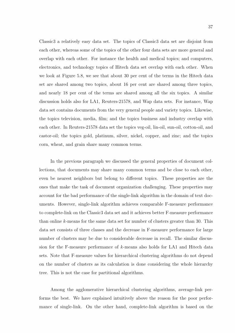
37

Classic3 a relatively easy data set. The topics of Classic3 data set are disjoint from

each other, whereas some of the topics of the other four data sets are more general and

overlap with each other. For instance the health and medical topics; and computers,

electronics, and technology topics of Hitech data set overlap with each other. When

we look at Figure 5.8, we see that about 30 per cent of the terms in the Hitech data

set are shared among two topics, about 16 per cent are shared among three topics,

and nearly 18 per cent of the terms are shared among all the six topics. A similar

discussion holds also for LA1, Reuters-21578, and Wap data sets. For instance, Wap

data set contains documents from the very general people and variety topics. Likewise,

the topics television, media, film; and the topics business and industry overlap with

each other. In Reuters-21578 data set the topics veg-oil, lin-oil, sun-oil, cotton-oil, and

castor-oil; the topics gold, platinum, silver, nickel, copper, and zinc; and the topics

corn, wheat, and grain share many common terms.

In the previous paragraph we discussed the general properties of document col-

lections, that documents may share many common terms and be close to each other,

even be nearest neighbors but belong to different topics. These properties are the

ones that make the task of document organization challenging. These properties may

account for the bad performance of the single-link algorithm in the domain of text doc-

uments. However, single-link algorithm achieves comparable F-measure performance

to complete-link on the Classic3 data set and it achieves better F-measure performance

than online k-means for the same data set for number of clusters greater than 30. This

data set consists of three classes and the decrease in F-measure performance for large

number of clusters may be due to considerable decrease in recall. The similar discus-

sion for the F-measure performance of k-means also holds for LA1 and Hitech data

sets. Note that F-measure values for hierarchical clustering algorithms do not depend

on the number of clusters as its calculation is done considering the whole hierarchy

tree. This is not the case for partitional algorithms.

Among the agglomerative hierarchical clustering algorithms, average-link per-

forms the best. We have explained intuitively above the reason for the poor perfor-

mance of single-link. On the other hand, complete-link algorithm is based on the

38

assumption that all the documents in the cluster are very similar to each other. This

assumption does not account for the high dimensional diverse nature of text document

domain, where each distinct word is considered as a different feature and context knowl-

edge such as synonyms, hyponyms, and hypernyms are not considered. Average-link

algorithm overcomes these problems by relying on more global properties to measure

cluster similarity. In this algorithm, similarity of two clusters is measured by taking

into account all the documents in both clusters.

Agglomerative algorithms are more common hierarchical clustering techniques

than the divisive ones since at each stage of a divisive algorithm we should consider

all possible ways of splitting data. This poses a great overhead for large data sets.

However, as we discussed in Chapter 3, Kaufman and Rousseeuw present a divisive

method in [35] that considers only a subset of the all possible partitions. We discussed

in Chapter 3 that we have modified this method slightly so that it becomes more robust

to outliers and our results reveal that it achieves similar performance to average-link

agglomerative hierarchical clustering algorithm.

When entropy, purity, and overall similarity metrics are considered online k-means

and bisecting k-means perform better than divisive hierarchical; and complete-link and

single-link agglomerative hierarchical clustering algorithms. They either achieve better

or similar performance to average-link algorithm.

In terms of the F-measure, bisecting k-means performs better than k-means and

similar to average-link and divisive hierarchical clustering algorithms. Calculating the

cosine similarity of a document to a cluster centroid is equivalent to calculating the

average similarity of the document to all the documents in that cluster. Hence, like

average-link and divisive hierarchical algorithms, k-means and its bisecting variant

also rely more on global properties to make decisions. A property of agglomerative and

divisive hierarchical algorithms that degrades their performance is that, in contrast to

k-means and bisecting k-means they do not revisit intermediate clusters for the purpose

of improving them, once they are constructed. K-means on the other hand has the

drawback that its performance depends very much on the parameter k and the initial

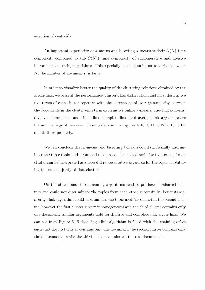
39

selection of centroids.

An important superiority of k-means and bisecting k-means is their O(N) time

complexity compared to the O(N2) time complexity of agglomerative and divisive

hierarchical clustering algorithms. This especially becomes an important criterion when

N , the number of documents, is large.

In order to visualize better the quality of the clustering solutions obtained by the

algorithms, we present the performance, cluster-class distribution, and most descriptive

five terms of each cluster together with the percentage of average similarity between

the documents in the cluster each term explains for online k-means, bisecting k-means;

divisive hierarchical; and single-link, complete-link, and average-link agglomerative

hierarchical algorithms over Classic3 data set in Figures 5.10, 5.11, 5.12, 5.13, 5.14,

and 5.15, respectively.

We can conclude that k-means and bisecting k-means could successfully discrim-

inate the three topics cisi, cran, and med. Also, the most-descriptive five terms of each

cluster can be interpreted as successful representative keywords for the topic constitut-

ing the vast majority of that cluster.

On the other hand, the remaining algorithms tend to produce unbalanced clus-

ters and could not discriminate the topics from each other successfully. For instance,

average-link algorithm could discriminate the topic med (medicine) in the second clus-

ter, however the first cluster is very inhomogeneous and the third cluster contains only

one document. Similar arguments hold for divisive and complete-link algorithms. We

can see from Figure 5.15 that single-link algorithm is faced with the chaining effect

such that the first cluster contains only one document, the second cluster contains only

three documents, while the third cluster contains all the rest documents.

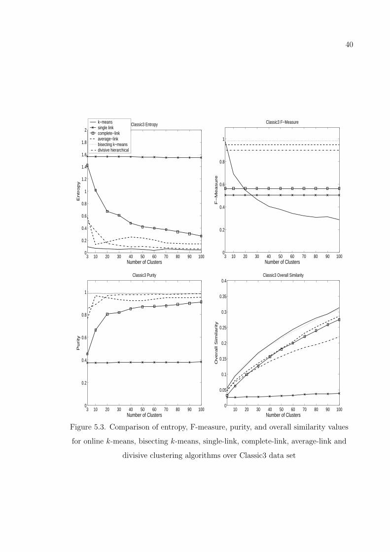
40

3 10 20 30 40 50 60 70 80 90 1000

0.2

0.4

0.6

0.8

1

1.2

1.4

1.6

1.8

2

Number of Clusters

En

tro

py

Classic3 Entropyk−meanssingle linkcomplete−linkaverage−linkbisecting k−meansdivisive hierarchical

3 10 20 30 40 50 60 70 80 90 1000

0.2

0.4

0.6

0.8

1

Number of Clusters

F−

Me

asu

re

Classic3 F−Measure

3 10 20 30 40 50 60 70 80 90 1000

0.2

0.4

0.6

0.8

1

Number of Clusters

Pu

rity

Classic3 Purity

10 20 30 40 50 60 70 80 90 1000

0.05

0.1

0.15

0.2

0.25

0.3

0.35

0.4

Number of Clusters

Ove

rall S

imila

rity

Classic3 Overall Similarity

Figure 5.3. Comparison of entropy, F-measure, purity, and overall similarity values

for online k-means, bisecting k-means, single-link, complete-link, average-link and

divisive clustering algorithms over Classic3 data set

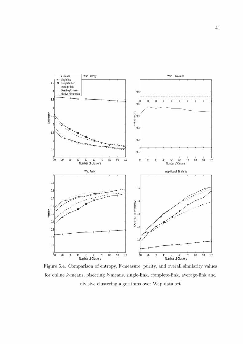
41

10 20 30 40 50 60 70 80 90 1000

0.5

1

1.5

2

2.5

3

3.5

4

4.5

Number of Clusters

En

tro

py

Wap Entropyk−meanssingle linkcomplete−linkaverage−linkbisecting k−meansdivisive hierarchical

10 20 30 40 50 60 70 80 90 100

0.1

0.2

0.3

0.4

0.5

0.6

Number of Clusters

F−

Measure

Wap F−Measure

10 20 30 40 50 60 70 80 90 1000

0.1

0.2

0.3

0.4

0.5

0.6

0.7

0.8

0.9

1

Number of Clusters

Pu

rity

Wap Purity

10 20 30 40 50 60 70 80 90 1000

0.1

0.2

0.3

0.4

0.5

Number of Clusters

Ove

rall S

imila

rity

Wap Overall Similarity



divisive clustering algorithms over Wap data set

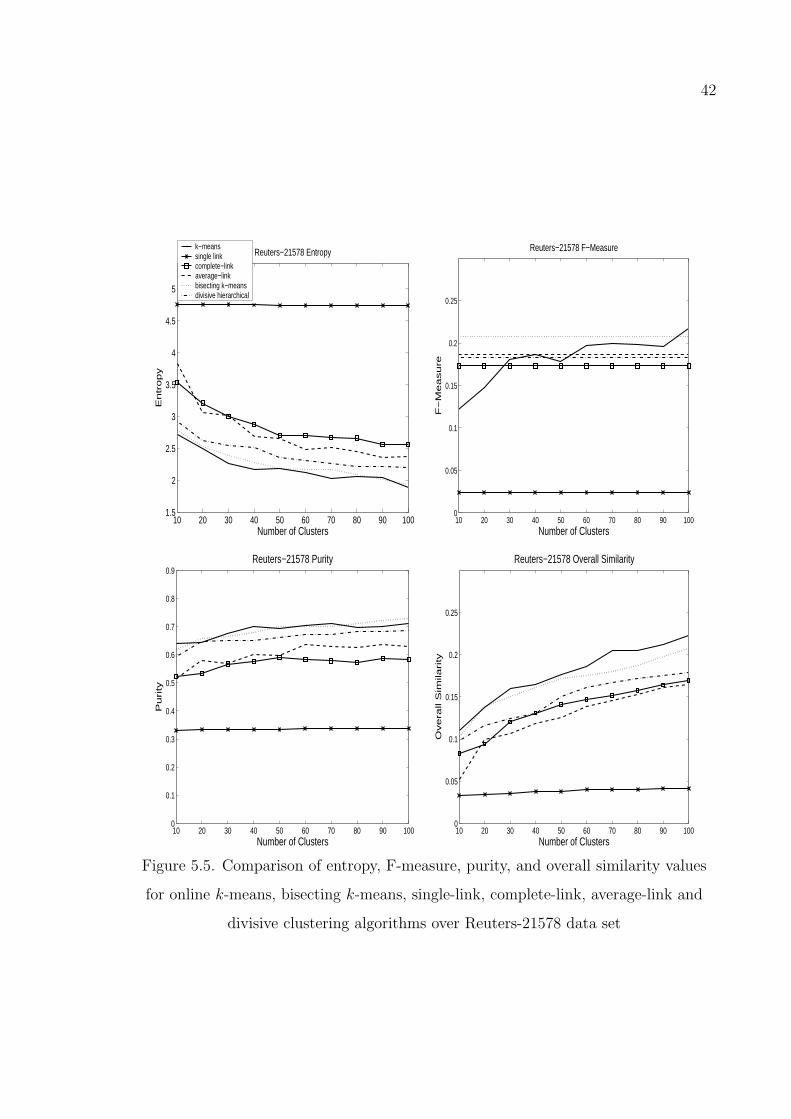
42

10 20 30 40 50 60 70 80 90 1001.5

2

2.5

3

3.5

4

4.5

5

Number of Clusters

En

tro

py

Reuters−21578 Entropyk−meanssingle linkcomplete−linkaverage−linkbisecting k−meansdivisive hierarchical

10 20 30 40 50 60 70 80 90 1000

0.05

0.1

0.15

0.2

0.25

Number of Clusters

F−

Measure

Reuters−21578 F−Measure

10 20 30 40 50 60 70 80 90 1000

0.1

0.2

0.3

0.4

0.5

0.6

0.7

0.8

0.9

Number of Clusters

Pu

rity

Reuters−21578 Purity

10 20 30 40 50 60 70 80 90 1000

0.05

0.1

0.15

0.2

0.25

Number of Clusters

Ove

rall S

imila

rity

Reuters−21578 Overall Similarity



divisive clustering algorithms over Reuters-21578 data set

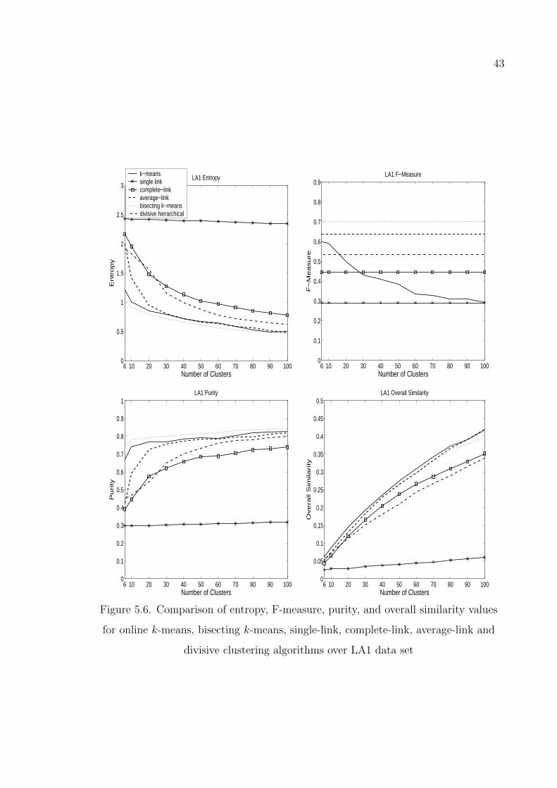
43

6 10 20 30 40 50 60 70 80 90 1000

0.5

1

1.5

2

2.5

3

Number of Clusters

En

tro

py

LA1 Entropyk−meanssingle linkcomplete−linkaverage−linkbisecting k−meansdivisive hierarchical

6 10 20 30 40 50 60 70 80 90 1000

0.1

0.2

0.3

0.4

0.5

0.6

0.7

0.8

0.9

Number of Clusters

F−

Me

asu

re

LA1 F−Measure

6 10 20 30 40 50 60 70 80 90 1000

0.1

0.2

0.3

0.4

0.5

0.6

0.7

0.8

0.9

1

Number of Clusters

Pu

rity

LA1 Purity

6 10 20 30 40 50 60 70 80 90 1000

0.05

0.1

0.15

0.2

0.25

0.3

0.35

0.4

0.45

0.5

Number of Clusters

Ove

rall S

imila

rity

LA1 Overall Similarity



divisive clustering algorithms over LA1 data set

44

6 10 20 30 40 50 60 70 80 90 1000

0.5

1

1.5

2

2.5

3

Number of Clusters

En

tro

py

Hitech Entropyk−meanssingle linkcomplete−linkaverage−linkbisecting k−meansdivisive hierarchical

6 10 20 30 40 50 60 70 80 90 1000

0.1

0.2

0.3

0.4

0.5

0.6

Number of Clusters

F−

Me

asu

re

Hitech F−Measure

6 10 20 30 40 50 60 70 80 90 1000

0.1

0.2

0.3

0.4

0.5

0.6

0.7

0.8

0.9

1

Number of Clusters

Pu

rity

Hitech Purity

6 10 20 30 40 50 60 70 80 90 1000

0.1

0.2

0.3

0.4

0.5

Number of Clusters

Ove

rall S

imila

rity

Hitech Overall Similarity



divisive clustering algorithms over Hitech data set

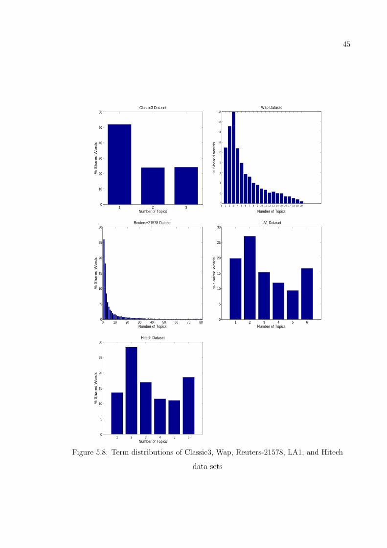
45

1 2 30

10

20

30

40

50

60Classic3 Dataset

Number of Topics

% S

hare

d W

ord

s

0 1 2 3 4 5 6 7 8 9 10 11 12 13 14 15 16 17 18 19 200

2

4

6

8

10

12

14

16

18Wap Dataset

Number of Topics%

Sh

are

d W

ord

s

0 10 20 30 40 50 60 70 800

5

10

15

20

25

30Reuters−21578 Dataset

Number of Topics

% S

hare

d W

ord

s

1 2 3 4 5 60

5

10

15

20

25

30LA1 Dataset

Number of Topics

% S

hare

d W

ord

s

1 2 3 4 5 60

5

10

15

20

25

30Hitech Dataset

Number of Topics

% S

hare

d W

ord

s

Figure 5.8. Term distributions of Classic3, Wap, Reuters-21578, LA1, and Hitech

data sets

46

Wap Classic3 Reut LA1 Hitech0

5

10

15

20

25

30

35Percent of Documents Whose Nearest Neighbor is of a Different Class

Data Sets

Pe

rce

nt

Figure 5.9. Per cent of documents in Classic3, Wap, Reuters-21578, LA1, and Hitech

document collections whose nearest neighbor belongs to a different class

47

In Appendix A, we present the same statistics for Hitech, LA1, Reuters-21578,

and Wap data sets as well. We display these statistics for number of clusters equal to

number of topics for Hitech and LA1 data sets. As Reuters-21578 and Wap data sets

contain large numbers of topics we present the statistics for ten clusters for these data

sets so that they are more comprehensible. It can be said that the algorithms display

similar behaviors for each data set. We can conclude that the wrong decisions taken

by agglomerative and divisive hierarchical algorithms in the initial steps degrade their

performance drastically, as they do not revisit intermediate clusters for the purpose

of improving them, once they are constructed, in contrast to k-means and bisecting

k-means. So, for the domain of text documents our results reveal that k-means and its

hierarchical variant bisecting k-means are more appropriate.

48

Statistics of k-means (K=3) for Classic3 Dataset

Number of: Documents = 3891 Topics = 3 Terms = 6729

Overall Similarity = 0.0398921 Overall F-measure = 0.982755

Overall Entropy = 0.0946597 Overall Purity = 0.988692

CID Size Sim Entropy Purity cisi cran med

0 1490 0.038 0.18 0.98 1455 17 18

1 1015 0.022 0.032 1 2 1 1012

2 1386 0.055 0.045 1 3 1380 3

CID Most Descriptive 5 Features

0 librari: 8.3% inform: 5.8% system: 3.3% index: 2.1% document: 1.8%

1 cell: 5.6% patient: 5.2% rat: 1.5% hormon: 1.3% growth: 1.3%

2 flow: 4.3% boundari: 3.2% layer: 3.1% pressur: 2.6% wing: 2.2%

Figure 5.10. The performance, cluster-class distribution, and most descriptive 5

features of each cluster, of the clustering solution obtained by k-means for Classic3

data set

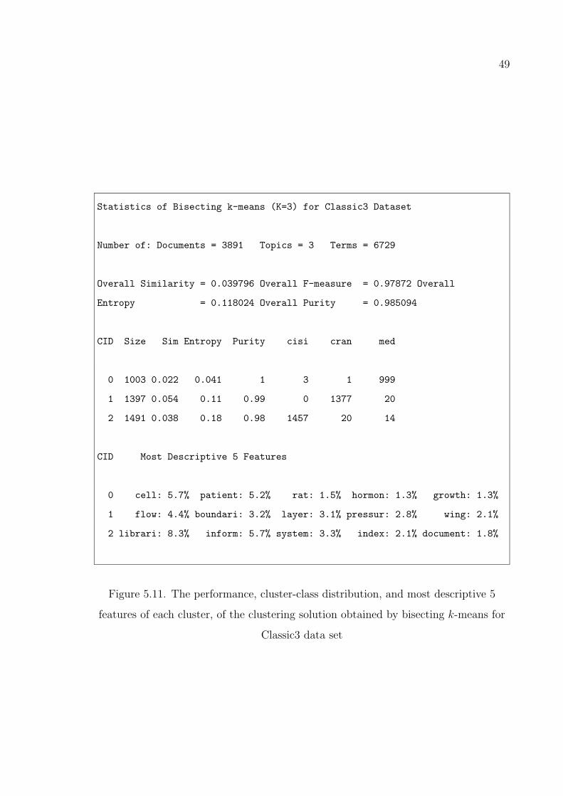
49

Statistics of Bisecting k-means (K=3) for Classic3 Dataset


Overall Similarity = 0.039796 Overall F-measure = 0.97872 Overall

Entropy = 0.118024 Overall Purity = 0.985094


0 1003 0.022 0.041 1 3 1 999

1 1397 0.054 0.11 0.99 0 1377 20

2 1491 0.038 0.18 0.98 1457 20 14


0 cell: 5.7% patient: 5.2% rat: 1.5% hormon: 1.3% growth: 1.3%

1 flow: 4.4% boundari: 3.2% layer: 3.1% pressur: 2.8% wing: 2.1%

2 librari: 8.3% inform: 5.7% system: 3.3% index: 2.1% document: 1.8%


features of each cluster, of the clustering solution obtained by bisecting k-means for

Classic3 data set

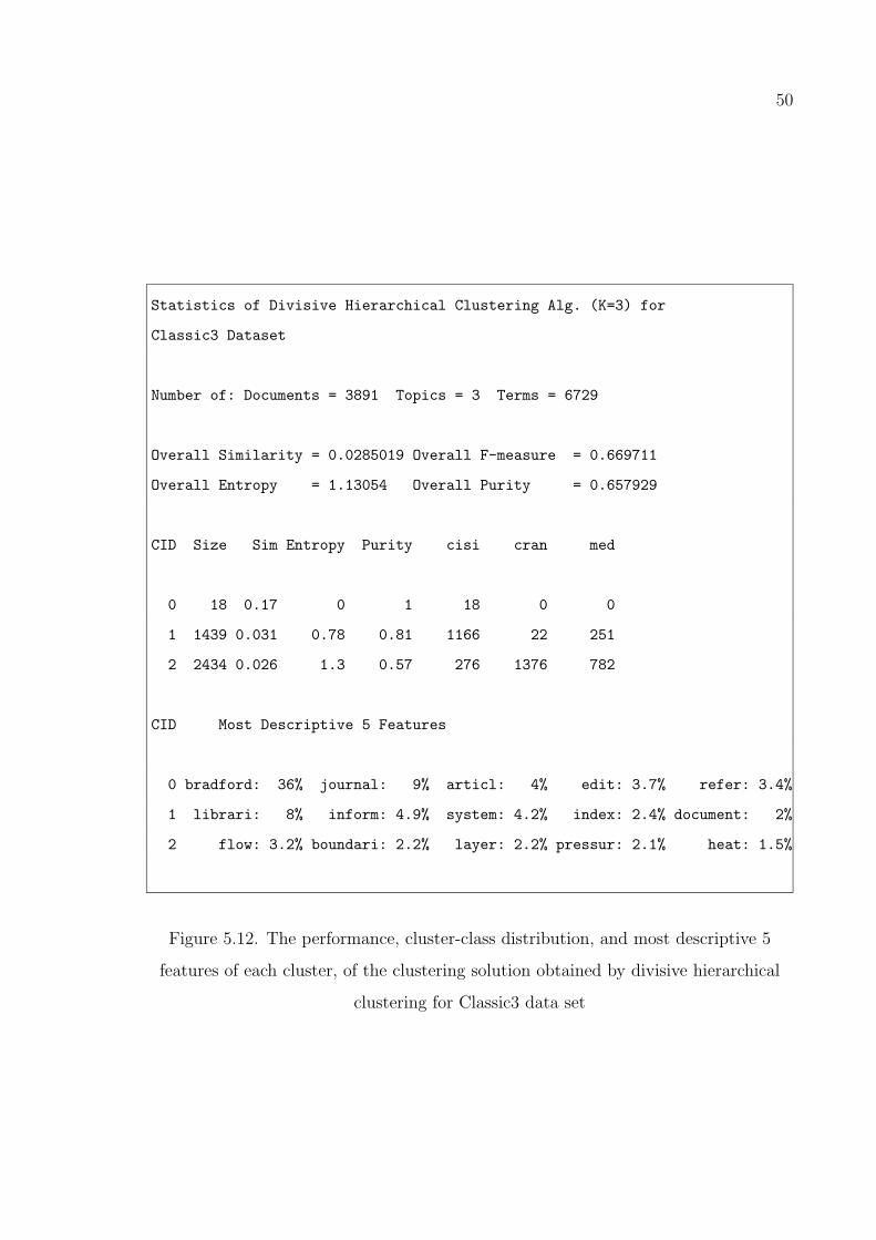
50

Statistics of Divisive Hierarchical Clustering Alg. (K=3) for

Classic3 Dataset





0 18 0.17 0 1 18 0 0

1 1439 0.031 0.78 0.81 1166 22 251

2 2434 0.026 1.3 0.57 276 1376 782


0 bradford: 36% journal: 9% articl: 4% edit: 3.7% refer: 3.4%

1 librari: 8% inform: 4.9% system: 4.2% index: 2.4% document: 2%

2 flow: 3.2% boundari: 2.2% layer: 2.2% pressur: 2.1% heat: 1.5%


features of each cluster, of the clustering solution obtained by divisive hierarchical

clustering for Classic3 data set

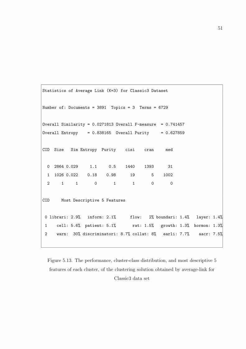
51

Statistics of Average Link (K=3) for Classic3 Dataset





0 2864 0.029 1.1 0.5 1440 1393 31

1 1026 0.022 0.18 0.98 19 5 1002

2 1 1 0 1 1 0 0


0 librari: 2.9% inform: 2.1% flow: 2% boundari: 1.4% layer: 1.4%

1 cell: 5.6% patient: 5.1% rat: 1.5% growth: 1.3% hormon: 1.3%

2 warn: 30% discriminatori: 8.7% collat: 8% earli: 7.7% aacr: 7.5%


features of each cluster, of the clustering solution obtained by average-link for

Classic3 data set

52

Statistics of Complete Link (K=3) for Classic3 Dataset





0 7 0.21 0 1 7 0 0

1 85 0.11 0 1 85 0 0

2 3799 0.02 1.6 0.37 1368 1398 1033


0 taxonomi: 17% dewei: 8.8% domain: 6.7% classif: 4.4% optim: 2%

1 librari: 52% public: 3% servic: 2.1% educ: 1.7% school: 1.3%

2 flow: 1.8% inform: 1.7% librari: 1.3% boundari: 1.2% system: 1.2%


features of each cluster, of the clustering solution obtained by complete-link for

Classic3 data set

53

Statistics of Single Link (K=3) for Classic3 Dataset





0 1 1 0 1 0 0 1

1 3 0.44 0.92 0.67 2 0 1

2 3887 0.02 1.6 0.38 1458 1398 1031


0 ceylon: 33% vector: 16% plasmodium: 15% host: 5.6% natur: 4.4%

1 echo: 34% delus: 13% ancient: 3.7% moral: 3.7% mental: 3.1%

2 librari: 2.3% inform: 1.7% flow: 1.7% system: 1.2% boundari: 1.1%


features of each cluster, of the clustering solution obtained by single-link for Classic3

data set

5.3. Evaluation of the Classification Techniques

5.3.1. Evaluation Metrics

To evaluate the performance of the supervised text classification techniques we

use the commonly used F1-measure, which is first introduced by van Rijsbergen [45].

54

F1-measure is a special case of the more general Fβ-measure defined as [1]:

Fβ =(β2 + 1)πρ

β2π + ρ(5.11)

where π is precision and ρ is recall. β can take values in the range [0, +∞]. It may be

interpreted as the relative degree of importance given to π and ρ. If β = 0, Fβ = π,

whereas if β = +∞ then Fβ = ρ. F1-measure combines recall and precision with equal

weight. It is equal to their harmonic mean:

F1 =2πρ

π + ρ(5.12)

Precision for class i is the ratio of correct assignments by the system divided by the

total number of assignments by the system to class i, whereas recall for class i is the

ratio of correct assignments by the system to class i divided by the total number of

correct assignments:

πi =TPi

TPi + FPi

(5.13)

ρi =TPi

TPi + FNi

(5.14)

Here, TPi (True Positives) is the number of documents assigned correctly to class i;

FPi (False Positives) is the number of documents that do not belong to class i but are

assigned to class i incorrectly by the classifier; and FNi (False Negatives) is the number

of documents that are not assigned to class i by the classifier but which actually belong

to class i.

The overall F1 measure score of the entire classification problem can be computed

by two different types of averages, micro-average and macro-average.

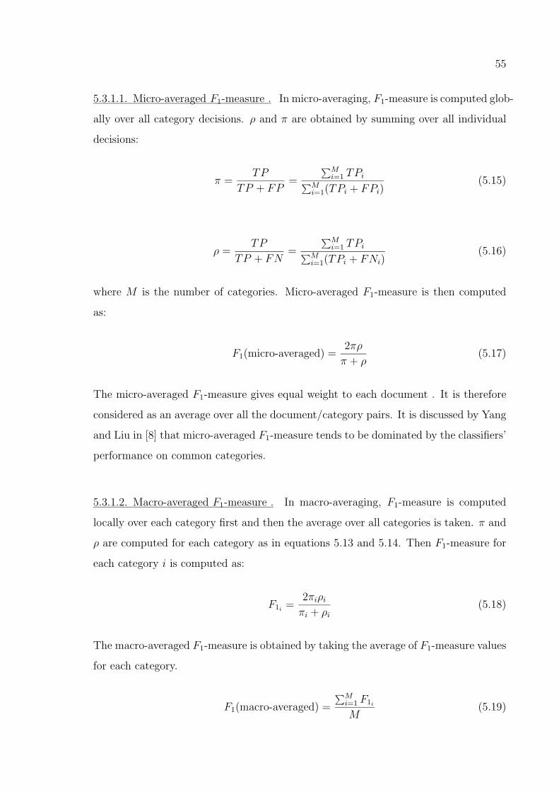
55

5.3.1.1. Micro-averaged F1-measure . In micro-averaging, F1-measure is computed glob-

ally over all category decisions. ρ and π are obtained by summing over all individual

decisions:

π =TP

TP + FP=

∑Mi=1 TPi∑M

i=1(TPi + FPi)(5.15)

ρ =TP

TP + FN=

∑Mi=1 TPi∑M

i=1(TPi + FNi)(5.16)

where M is the number of categories. Micro-averaged F1-measure is then computed

as:

F1(micro-averaged) =2πρ

π + ρ(5.17)

The micro-averaged F1-measure gives equal weight to each document . It is therefore

considered as an average over all the document/category pairs. It is discussed by Yang

and Liu in [8] that micro-averaged F1-measure tends to be dominated by the classifiers’

performance on common categories.

5.3.1.2. Macro-averaged F1-measure . In macro-averaging, F1-measure is computed

locally over each category first and then the average over all categories is taken. π and

ρ are computed for each category as in equations 5.13 and 5.14. Then F1-measure for

each category i is computed as:

F1i=

2πiρi

πi + ρi

(5.18)

The macro-averaged F1-measure is obtained by taking the average of F1-measure values

for each category.

F1(macro-averaged) =

∑Mi=1 F1i

M(5.19)

56

where M is total number of categories. Macro-averaged F1-measure gives equal weight

to each category, regardless of its frequency. It is discussed by Yang and Liu in [8] that

macro-averaged F1-measure is influenced more by the classifiers performance on rare

categories.

So, we provide both measurement scores to be more informative.

5.3.2. Results and Discussion

In this section we present the micro-averaged and macro-averaged F1-measure

results of naive Bayes classifier relying on multivariate Bernoulli model, traditional

k-NN, weighted k-NN, and SVM.

We used SV M light package, version 5.00 [40], to train and test the SVM classifier.

We performed experiments on SVM with linear kernel; polynomial kernel of degrees 2,

3, 4, 5, 6, and 7; and RBF kernel with variances 0.2, 0.4, 0.6, 0.8, 1.0, 1.2, and 1.4.

Tables 5.2 and 5.3 display micro-averaged and macro-averaged F1-measure results, re-

spectively, for SVM with polynomial kernel. Tables 5.4 and 5.5 display micro-averaged

and macro-averaged F1-measure results, respectively, for SVM with RBF kernel.

Table 5.2. Micro-averaged F1-measure results for SVM with polynomial kernel of

degrees 1, 2, 3, 4, 5, 6, and 7

Data set 1 2 3 4 5 6 7

Classic3 0.970 0.994 0.994 0.994 0.994 0.992 0.991

Hitech 0.728 0.736 0.727 0.719 0.712 0.695 0.674

LA1 0.884 0.882 0.882 0.874 0.832 0.831 0.786

Reuters-21578 0.823 0.813 0.802 0.780 0.756 0.710 0.659

Wap 0.839 0.838 0.838 0.822 0.802 0.770 0.702

57

Table 5.3. Macro-averaged F1-measure results for SVM with polynomial kernel of

degrees 1, 2, 3, 4, 5, 6, and 7

Data set 1 2 3 4 5 6 7

Classic3 0.968 0.994 0.994 0.994 0.994 0.992 0.991

Hitech 0.662 0.666 0.641 0.627 0.608 0.576 0.555

LA1 0.847 0.843 0.839 0.825 0.766 0.764 0.708

Reuters-21578 0.503 0.486 0.474 0.461 0.446 0.422 0.412

Wap 0.662 0.658 0.657 0.617 0.583 0.546 0.491

Table 5.4. Micro-averaged F1-measure results for SVM with RBF kernel with

γ = 0.2, 0.4, 0.6, 0.8, 1.0, 1.2, 1.4

Data set 0.2 0.4 0.6 0.8 1.0 1.2 1.4

Classic3 0.993 0.994 0.994 0.994 0.993 0.993 0.993

Hitech 0.736 0.731 0.725 0.721 0.721 0.716 0.711

LA1 0.882 0.878 0.876 0.873 0.864 0.857 0.849

Reuters-21578 0.814 0.806 0.794 0.777 0.758 0.733 0.704

Wap 0.839 0.834 0.832 0.821 0.813 0.801 0.781

Table 5.5. Macro-averaged F1-measure results for SVM with RBF kernel with

γ = 0.2, 0.4, 0.6, 0.8, 1.0, 1.2, 1.4

Data set 0.2 0.4 0.6 0.8 1.0 1.2 1.4

Classic3 0.994 0.994 0.994 0.994 0.993 0.993 0.993

Hitech 0.667 0.653 0.636 0.619 0.616 0.609 0.598

LA1 0.840 0.833 0.828 0.823 0.806 0.795 0.784

Reuters-21578 0.485 0.464 0.433 0.412 0.388 0.361 0.337

Wap 0.662 0.642 0.637 0.609 0.593 0.577 0.551

58

In the training phase the parameter C, which is the trade-off between training

error and margin, is left to its default value. In the SV M light system, the default value

of C is defined to be equal to the reciprocal of the average Euclidean norm of training

examples. We did not perform experiments with different C values as the results we

obtained are satisfactory. From the results we can say that generally linear kernel or

polynomial kernel of degree 2 lead to better performance. However, performance does

not change drastically with the complexity of the model. Effect of the degree of the

polynomial kernel and the variance of the RBF kernel of SVM to the F1-measure scores

are displayed in Figures 5.16 and 5.17 respectively.

Tables 5.6 and 5.7 display the micro-averaged and macro-averaged F1-measure

results of the supervised techniques we evaluated. For traditional k-NN and weighted

k-NN we performed experiments for k values starting with 5 and incrementing by 5

till k = 60. We report the results for the optimum k value, and report that k value

in parentheses as well. Likewise, for SVM we report the best results obtained and the

model leading to those results in parentheses.

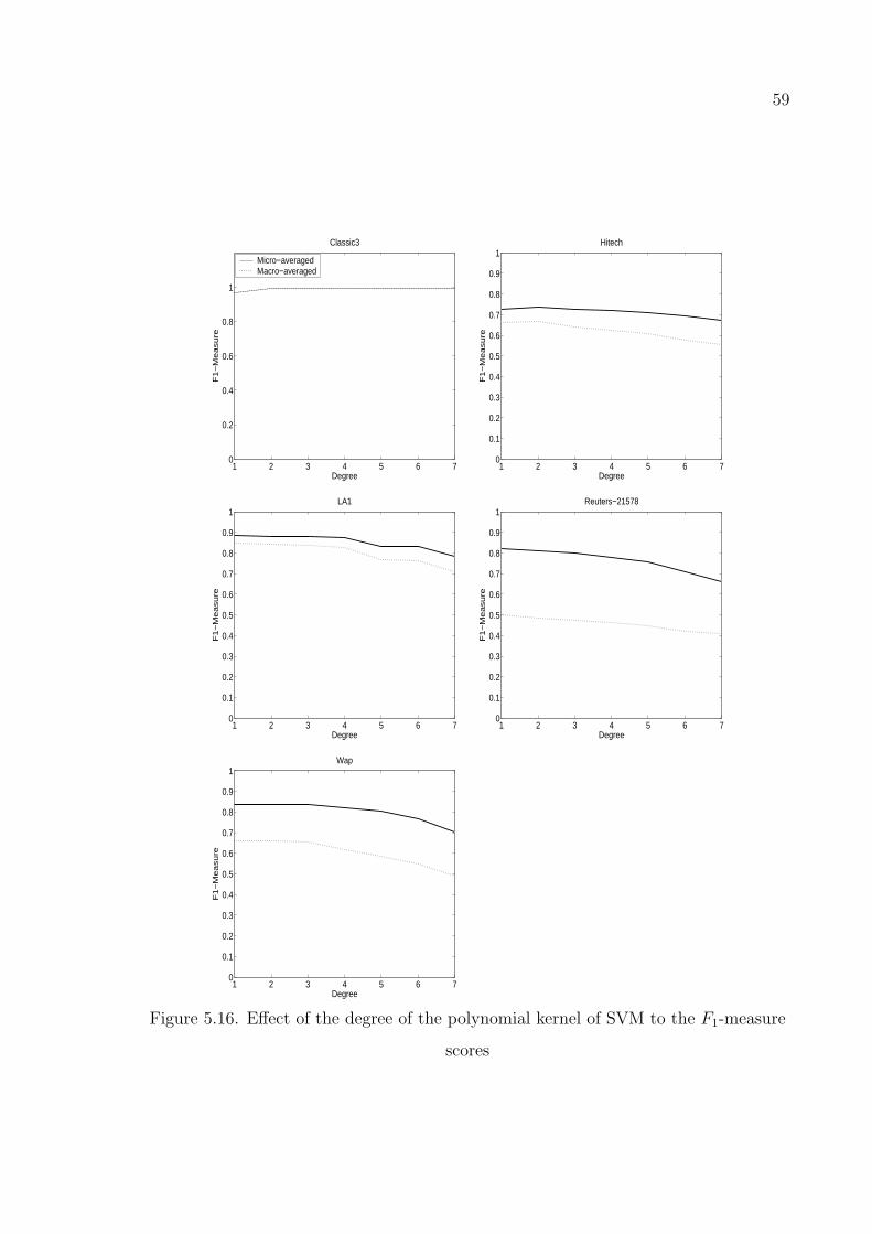
59

1 2 3 4 5 6 70

0.2

0.4

0.6

0.8

1

Degree

F1−

Measure

Classic3

Micro−averagedMacro−averaged

1 2 3 4 5 6 70

0.1

0.2

0.3

0.4

0.5

0.6

0.7

0.8

0.9

1

DegreeF

1−

Measure

Hitech

1 2 3 4 5 6 70

0.1

0.2

0.3

0.4

0.5

0.6

0.7

0.8

0.9

1

Degree

F1−

Measure

LA1

1 2 3 4 5 6 70

0.1

0.2

0.3

0.4

0.5

0.6

0.7

0.8

0.9

1

Degree

F1−

Measure

Reuters−21578

1 2 3 4 5 6 70

0.1

0.2

0.3

0.4

0.5

0.6

0.7

0.8

0.9

1

Degree

F1−

Measure

Wap

Figure 5.16. Effect of the degree of the polynomial kernel of SVM to the F1-measure

scores

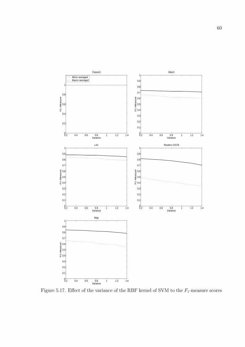
60

0.2 0.4 0.6 0.8 1 1.2 1.40

0.2

0.4

0.6

0.8

1

Variance

F1−

Measure

Classic3

Micro−averagedMacro−averaged

0.2 0.4 0.6 0.8 1 1.2 1.40

0.1

0.2

0.3

0.4

0.5

0.6

0.7

0.8

0.9

1

VarianceF

1−

Measure

Hitech

0.2 0.4 0.6 0.8 1 1.2 1.40

0.1

0.2

0.3

0.4

0.5

0.6

0.7

0.8

0.9

1

Variance

F1−

Measure

LA1

0.2 0.4 0.6 0.8 1 1.2 1.40

0.1

0.2

0.3

0.4

0.5

0.6

0.7

0.8

0.9

1

Variance

F1−

Measure

Reuters−21578

0.2 0.4 0.6 0.8 1 1.2 1.40

0.1

0.2

0.3

0.4

0.5

0.6

0.7

0.8

0.9

1

Variance

F1−

Measure

Wap

Figure 5.17. Effect of the variance of the RBF kernel of SVM to the F1-measure scores

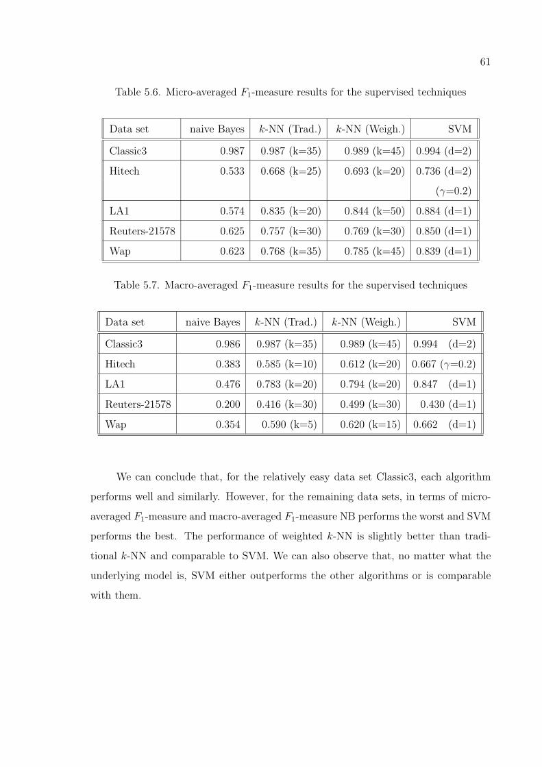
61

Table 5.6. Micro-averaged F1-measure results for the supervised techniques

Data set naive Bayes k-NN (Trad.) k-NN (Weigh.) SVM

Classic3 0.987 0.987 (k=35) 0.989 (k=45) 0.994 (d=2)

Hitech 0.533 0.668 (k=25) 0.693 (k=20) 0.736 (d=2)

(γ=0.2)

LA1 0.574 0.835 (k=20) 0.844 (k=50) 0.884 (d=1)

Reuters-21578 0.625 0.757 (k=30) 0.769 (k=30) 0.850 (d=1)

Wap 0.623 0.768 (k=35) 0.785 (k=45) 0.839 (d=1)

Table 5.7. Macro-averaged F1-measure results for the supervised techniques

Data set naive Bayes k-NN (Trad.) k-NN (Weigh.) SVM

Classic3 0.986 0.987 (k=35) 0.989 (k=45) 0.994 (d=2)

Hitech 0.383 0.585 (k=10) 0.612 (k=20) 0.667 (γ=0.2)

LA1 0.476 0.783 (k=20) 0.794 (k=20) 0.847 (d=1)

Reuters-21578 0.200 0.416 (k=30) 0.499 (k=30) 0.430 (d=1)

Wap 0.354 0.590 (k=5) 0.620 (k=15) 0.662 (d=1)

We can conclude that, for the relatively easy data set Classic3, each algorithm

performs well and similarly. However, for the remaining data sets, in terms of micro-

averaged F1-measure and macro-averaged F1-measure NB performs the worst and SVM

performs the best. The performance of weighted k-NN is slightly better than tradi-

tional k-NN and comparable to SVM. We can also observe that, no matter what the

underlying model is, SVM either outperforms the other algorithms or is comparable

with them.

62

6. COMPARISON OF THE SUPERVISED AND

UNSUPERVISED METHODS

Comparison of the unsupervised techniques [18] and comparison of the supervised

techniques [8] have been performed in the literature. However to our knowledge the

two approaches have not been compared with each other. In this chapter we compare

the quality of the clusters produced by the two approaches. The classification solutions

obtained by the supervised techniques are considered as if they were clustering solutions

and they are evaluated by using the evaluation metrics that are used to evaluate the

performance of the clustering algorithms. The clustering algorithms on the other hand

are ran for number of clusters equal to the number of pre-defined categories in each

document corpus. Tables 6.1, 6.2, 6.3, 6.4, and 6.5 display the results for Classic3,

Hitech, LA1, Reuters-21578, and Wap data sets respectively. We do not present the

results for the single-link algorithm as it is shown to be a very bad performer in the

previous chapter.


supervised techniques for Classic3

Algorithm Entropy Purity Overall F-Measure

Similarity

average-link 0.574 0.767 0.047 0.817

bisecting k-means 0.098 0.987 0.055 0.983

complete-link 1.423 0.455 0.032 0.520

divisive 0.503 0.855 0.051 0.865

k-means 0.093 0.987 0.055 0.984

k-NN (Traditional) 0.093 0.987 0.055 0.983

k-NN (Weighted) 0.078 0.989 0.055 0.986

NB 0.091 0.987 0.055 0.983

SVM 0.047 0.994 0.055 0.991

63


supervised techniques for Hitech


Similarity

average-link 2.167 0.341 0.068 0.308


complete-link 2.067 0.385 0.061 0.356

divisive 1.732 0.485 0.068 0.453

k-means 1.523 0.558 0.083 0.497

k-NN (Traditional) 1.394 0.670 0.078 0.593

k-NN (Weighted) 1.308 0.695 0.079 0.626

NB 1.832 0.536 0.061 0.485

SVM 1.181 0.738 0.079 0.666


supervised techniques for LA1


Similarity

average-link 2.000 0.424 0.050 0.372


complete-link 2.167 0.391 0.043 0.344

divisive 1.916 0.451 0.055 0.410

k-means 1.210 0.671 0.061 0.597

k-NN (Traditional) 0.831 0.835 0.062 0.763

k-NN (Weighted) 0.781 0.845 0.062 0.773

NB 1.660 0.574 0.049 0.525

SVM 0.618 0.884 0.062 0.816

64


supervised techniques for Reuters-21578


Similarity

average-link 2.353 0.637 0.161 0.171


complete-link 2.563 0.587 0.164 0.164

divisive 2.209 0.682 0.175 0.178

k-means 2.049 0.701 0.212 0.196

k-NN (Traditional) 2.200 0.739 0.108 0.247

k-NN (Weighted) 2.092 0.748 0.115 0.264

NB 3.267 0.627 0.067 0.111

SVM 1.982 0.879 0.192 0.297


supervised techniques for Wap


Similarity

average-link 1.282 0.616 0.182 0.453


complete-link 1.987 0.462 1.151 0.332

divisive 1.876 0.521 0.088 0.350

k-means 1.173 0.662 0.193 0.473

k-NN (Traditional) 1.026 0.769 0.142 0.580

k-NN (Weighted) 0.954 0.787 0.151 0.597

NB 1.552 0.658 0.119 0.463

SVM 0.706 0.846 0.165 0.652

65

Different from the unsupervised techniques, the supervised techniques use class

label information in addition to the similarity information between documents. For this

reason, it is expected that the clusters (groups) obtained by the supervised techniques

are of higher quality compared to the unsupervised techniques. However, we can ob-

serve from the results that the best performers of the unsupervised techniques k-means

and bisecting k-means achieve generally better performance than NB and not much

worse performance than k-NN, which are supervised techniques, in terms of entropy,

purity, overall similarity and F -measure. SVM achieves the highest performance in

terms of entropy, purity, and F -measure. Another observation is that, compared with

the supervised techniques the unsupervised techniques generally achieve higher overall

similarity performance. This is due to the fact that they make decisions depending only

on the similarity information between documents. On the other hand the supervised

techniques use a labelled training set. This observation has made us think that there

may be some outliers in the labelled training set that lead to decrease in the overall

similarity of the clusters obtained and unsupervised techniques can be used to enhance

the task of pre-defining categories and labelling documents in the training set.

66

7. CONCLUSIONS AND FUTURE WORK

The advances in technology of computers and electronics, the increasing popular-

ity of the Internet and the WWW have lead to vast amounts of increase in electronic

text information. In order to browse text databases and extract relevant information

fast, efficiently, and correctly organizing digital text documents automatically has be-

come an important research issue. There are two major machine learning approaches

for document organization, supervised and unsupervised. In this study we present an

experimental evaluation of these two major paradigms.

We discuss, different alternatives for document representation and explain our

methodology in Chapter 2. We chose to use the “bag-of-words” representation, where

each distinct stemmed word is defined as a term. Stopwords and mark-up tags are

removed, words are stemmed by using Porter’s stemming algorithm, and dimensionality

is reduced by the unsupervised DF Thresholding technique.

After the preprocessing phase, we implement and apply the leading unsupervised

and supervised algorithms to five standard document corpora. Among the unsupervised

algorithms, we evaluate the most popular partitional clustering technique k-means, its

variant bisecting k-means, the main agglomerative hierarchical clustering techniques;

single-link, complete-link, and average-link, and divisive hierarchical clustering tech-

nique which to our knowledge has not been used to cluster documents previously. We

conclude that among the hierarchical clustering algorithms the average-link algorithm

achieves the best performance and the divisive algorithm achieves similar performance.

The reason for the worse performance of the single-link and the complete-link algo-

rithms is that, they depend on assumptions far from reality for the nature of text

document collections. The single-link algorithm assumes that nearest neighbors be-

long to the same class and the complete-link algorithm assumes that documents in a

cluster are very similar to each other. We presented a discussion in Chapter 5 that

documents may share many common terms and be close to each other, even be nearest

neighbors but belong to different categories. These properties are the ones that make

67

the task of document organization challenging. In the domain of text documents, the

number of documents, N , is usually very large. In this case, k-means and bisecting

k-means can be more favorable than agglomerative and divisive hierarchical clustering

algorithms as they have O(N) time complexity in contrast to the O(N2) time complex-

ity of agglomerative and divisive hierarchical clustering algorithms. On the other hand,

performance of k-means and bisecting k-means depends very much on the parameter

k and the initial selection of centroids. In Chapter 5 and in Appendix A we illus-

trate the performance of the unsupervised techniques over the data sets by presenting

some statistics where we observe that k-means and bisecting k-means usually better

discriminate between the actual classes, while the hierarchical techniques may lead to

rather inhomogeneous and unbalanced clusters. Especially the single-link algorithm

has a tendency to suffer from the chaining effect.

We evaluate the performance of multivariate Bernoulli model of NB, traditional

k-NN, weighted k-NN, and SVM supervised techniques. Our results reveal that,

NB achieves the lowest performance, while SVM performs the best. Weighted k-

NN achieves comparable performance to SVM, and traditional k-NN performs slightly

worse than weighted k-NN. The reasons for the poor performance of NB may be the

boolean vector representation of the documents and the unrealistic naive assumption

that the probability of each term being present in a document is only dependent on

the category of the documents and independent from the presence of other terms in

the document.

As a conclusion we can say that, for unsupervised document clustering k-means

and its variant bisecting k-means are more appropriate than the agglomerative and

divisive hierarchical clustering techniques both in terms of time complexity and the

quality of the clusters produced. Agglomerative and divisive hierarchical clustering

algorithms generally produce unbalanced, inhomogeneous clusters. Although divisive

hierarchical clustering is not as common as agglomerative approach it does not produce

worse results. On the other hand for supervised document categorization the method

with best performance is SVM and NB approach performs poorly.

68

In Chapter 6 we compared the unsupervised techniques with the supervised tech-

niques in terms of the quality of the clusters they produce. We considered the classifica-

tion solutions obtained by the supervised techniques as if they were clustering solutions

and likewise evaluated the unsupervised algorithms for number of clusters equal to the

pre-defined number of categories for each data set. From these experiments, different

from our expectations we conclude that although k-means and bisecting k-means are

unsupervised techniques they produce clusters of better quality than NB, and not much

worse than k-NN and SVM. In addition, clusters produced by unsupervised techniques

have generally greater overall similarity than the clusters produced by the supervised

techniques. The reason may be due to outliers in the labelled documents. For the

supervised techniques to be applied to document categorization, categories should be

pre-defined and there should be a training set of labelled documents. We discuss that

defining the categories in advance and preparing a labelled training set is a challenging,

error prone, and subjective task especially in dynamic text environments such as the

WWW. We discuss the inter-indexer inconsistency phenomenon where two different

indexers may decide to label a document under different categories, depending on their

subjective opinion. Therefore, we suggest to use unsupervised clustering before apply-

ing supervised classification to enhance pre-definition of categories and preparation of

labelled training set. Given a document corpus a clustering solution can be obtained

and the human indexer can be presented with most descriptive terms of each cluster

representative as a suggestion for keywords of the cluster (category). The indexer can

be informed about the documents in each cluster which have relatively small average

pairwise similarity to the other documents in the cluster. This small average pairwise

similarity may be an indication of overlapping clusters or outlier documents in the

cluster.

As future work, we will work on a hybrid approach to organize text documents

that incorporates the strengths of supervised and unsupervised paradigms. This ap-

proach will start in an unsupervised manner without pre-defined categories and labelled

data and in a later phase will incorporate the supervised approach. Further future plans

are to integrate context knowledge such as word synonyms, hypernyms, hyponyms, and

phrases into the supervised and unsupervised techniques; to evaluate the techniques

69

for documents in Turkish and study the effects of language in the performance of the

supervised and unsupervised techniques; and to gather the source codes we have imple-

mented into a publicly available toolkit for document preprocessing and representation;

classification, and clustering.

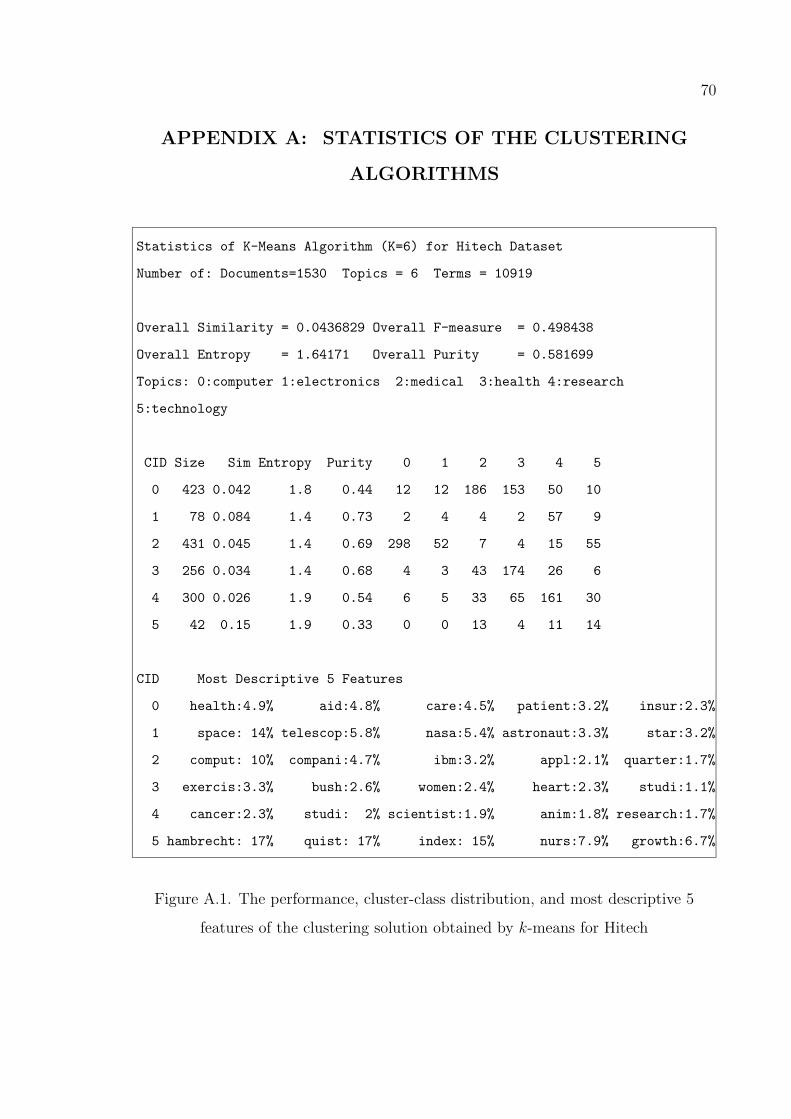
70

APPENDIX A: STATISTICS OF THE CLUSTERING

ALGORITHMS

Statistics of K-Means Algorithm (K=6) for Hitech Dataset

Number of: Documents=1530 Topics = 6 Terms = 10919



Topics: 0:computer 1:electronics 2:medical 3:health 4:research

5:technology

CID Size Sim Entropy Purity 0 1 2 3 4 5

0 423 0.042 1.8 0.44 12 12 186 153 50 10

1 78 0.084 1.4 0.73 2 4 4 2 57 9

2 431 0.045 1.4 0.69 298 52 7 4 15 55

3 256 0.034 1.4 0.68 4 3 43 174 26 6

4 300 0.026 1.9 0.54 6 5 33 65 161 30

5 42 0.15 1.9 0.33 0 0 13 4 11 14


0 health:4.9% aid:4.8% care:4.5% patient:3.2% insur:2.3%

1 space: 14% telescop:5.8% nasa:5.4% astronaut:3.3% star:3.2%

2 comput: 10% compani:4.7% ibm:3.2% appl:2.1% quarter:1.7%

3 exercis:3.3% bush:2.6% women:2.4% heart:2.3% studi:1.1%

4 cancer:2.3% studi: 2% scientist:1.9% anim:1.8% research:1.7%

5 hambrecht: 17% quist: 17% index: 15% nurs:7.9% growth:6.7%


features of the clustering solution obtained by k-means for Hitech

71

Statistics of Bisecting K-Means Algorithm (K=6) for Hitech Dataset





5:technology


0 333 0.045 1.4 0.69 231 25 3 5 16 53

1 428 0.042 1.7 0.45 5 1 193 155 52 22

2 112 0.055 1.6 0.68 4 9 8 6 76 9

3 162 0.036 2.1 0.37 7 3 32 51 60 9

4 363 0.027 1.8 0.5 4 4 44 183 109 19

5 132 0.082 1.8 0.54 71 34 6 2 7 12


0 comput: 13% ibm:4.8% appl:3.3% compani: 3.1% system:1.3%

1 health:4.8% aid:4.6% care:4.4% patient: 3.4% insur:2.2%

2 space:8.2% farlei:6.6% telescop:4.5% nasa: 3.9% earth:3.1%

3 cancer:6.4% bush:5.5% gene:3.3% cell: 3.1% diseas:2.2%

4 studi:2.2% exercis:1.9% women:1.3% water: 1.2% research:0.85%

5 quarter:8.6% stock:5.4% compani: 5% million: 4.5% share:3.5%



Hitech data set

72

Statistics of Divisive Hierarchical Algorithm (K=6) for Hitech

Dataset





5:technology


0 988 0.024 2.4 0.32 318 76 166 125 186 117

1 490 0.032 1.5 0.54 0 0 99 266 121 4

2 5 0.28 0.72 0.8 0 0 1 0 4 0

3 13 0.16 2 0.31 2 0 0 4 4 3

4 32 0.15 1.3 0.63 0 0 20 7 5 0

5 2 0.73 0 1 2 0 0 0 0 0


0 comput:4.1% compani:2.3% ibm:1.2% million:1.1% appl:0.8%

1 aid: 4% health:3.5% patient: 3% care:2.7% infect:1.7%

2 bird: 24% dinosaur: 12% parrot: 12% hunter:6.4% ancestor: 3%

3 fax: 27% label: 19% wine:4.8% printer:3.9% grape:2.5%

4 suicid: 18% kevorkian: 18% casolaro: 4% banoff:3.3% sutherland:3.2%

5 novell: 59% banyan: 20% microsoft: 2% digit:1.8% acquisit:0.91%



clustering for Hitech data set

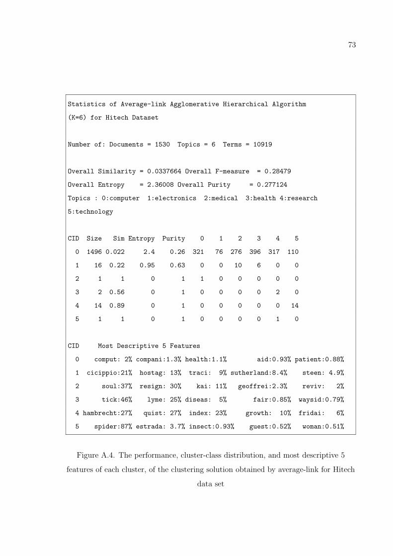
73

Statistics of Average-link Agglomerative Hierarchical Algorithm

(K=6) for Hitech Dataset




Topics : 0:computer 1:electronics 2:medical 3:health 4:research

5:technology


0 1496 0.022 2.4 0.26 321 76 276 396 317 110

1 16 0.22 0.95 0.63 0 0 10 6 0 0

2 1 1 0 1 1 0 0 0 0 0

3 2 0.56 0 1 0 0 0 0 2 0

4 14 0.89 0 1 0 0 0 0 0 14

5 1 1 0 1 0 0 0 0 1 0


0 comput: 2% compani:1.3% health:1.1% aid:0.93% patient:0.88%

1 cicippio:21% hostag: 13% traci: 9% sutherland:8.4% steen: 4.9%

2 soul:37% resign: 30% kai: 11% geoffrei:2.3% reviv: 2%

3 tick:46% lyme: 25% diseas: 5% fair:0.85% waysid:0.79%

4 hambrecht:27% quist: 27% index: 23% growth: 10% fridai: 6%

5 spider:87% estrada: 3.7% insect:0.93% guest:0.52% woman:0.51%


features of each cluster, of the clustering solution obtained by average-link for Hitech

data set

74

Statistics of Complete-link Agglomerative Hierarchical Algorithm






5:technology


0 59 0.089 0.9 0.85 50 1 2 0 3 3

1 37 0.066 1.5 0.59 0 0 5 9 22 1

2 47 0.082 1.7 0.45 21 17 0 1 2 6

3 24 0.12 2 0.54 1 3 1 4 13 2

4 55 0.056 2.2 0.33 7 0 6 18 17 7

5 1308 0.022 2.4 0.28 243 55 272 370 263 105


0 comput: 10% pc:5.2% disk:4.5% box:3.9% program:2.2%

1 anim:9.4% speci:4.6% bee:3.7% collagen:3.1% bird:2.3%

2 stock: 12% electron:5.6% trade:3.9% exchang:2.4% compani:2.4%

3 quak: 11% earthquak:8.1% fault:7.1% volcano:3.3% erupt:2.9%

4 pyramid: 7% nuclear:6.5% lab:2.7% ey:2.4% uranium:2.3%

5 comput:1.5% health:1.4% compani:1.2% aid:1.2% care:1.1%



Hitech data set

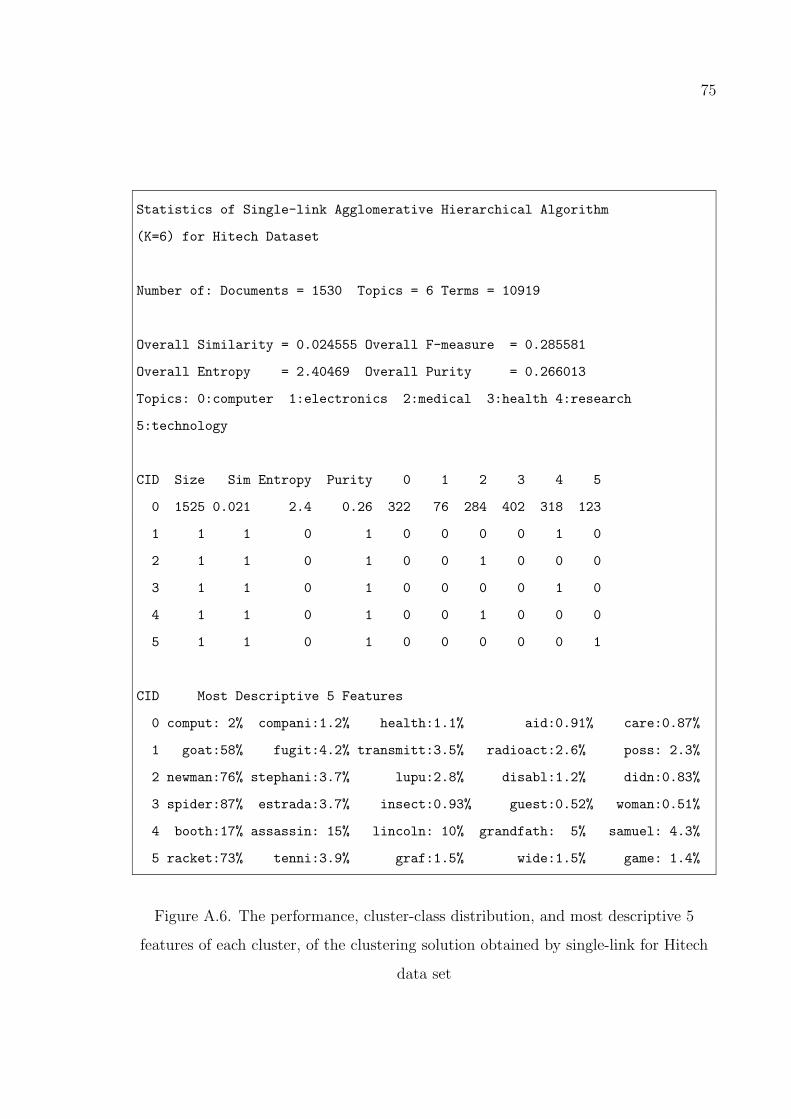
75

Statistics of Single-link Agglomerative Hierarchical Algorithm






5:technology


0 1525 0.021 2.4 0.26 322 76 284 402 318 123

1 1 1 0 1 0 0 0 0 1 0

2 1 1 0 1 0 0 1 0 0 0

3 1 1 0 1 0 0 0 0 1 0

4 1 1 0 1 0 0 1 0 0 0

5 1 1 0 1 0 0 0 0 0 1


0 comput: 2% compani:1.2% health:1.1% aid:0.91% care:0.87%

1 goat:58% fugit:4.2% transmitt:3.5% radioact:2.6% poss: 2.3%

2 newman:76% stephani:3.7% lupu:2.8% disabl:1.2% didn:0.83%

3 spider:87% estrada:3.7% insect:0.93% guest:0.52% woman:0.51%

4 booth:17% assassin: 15% lincoln: 10% grandfath: 5% samuel: 4.3%

5 racket:73% tenni:3.9% graf:1.5% wide:1.5% game: 1.4%


features of each cluster, of the clustering solution obtained by single-link for Hitech

data set

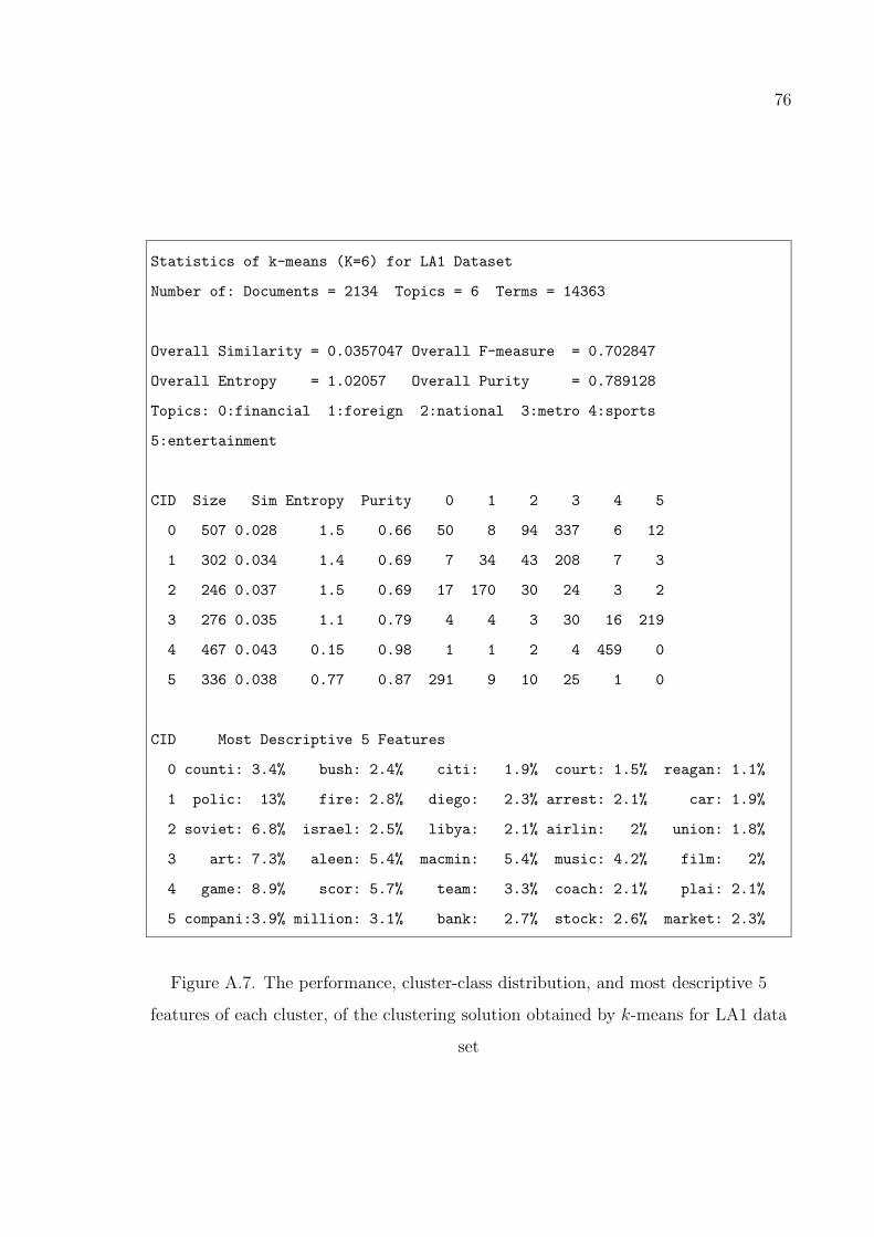
76

Statistics of k-means (K=6) for LA1 Dataset




Topics: 0:financial 1:foreign 2:national 3:metro 4:sports

5:entertainment


0 507 0.028 1.5 0.66 50 8 94 337 6 12

1 302 0.034 1.4 0.69 7 34 43 208 7 3

2 246 0.037 1.5 0.69 17 170 30 24 3 2

3 276 0.035 1.1 0.79 4 4 3 30 16 219

4 467 0.043 0.15 0.98 1 1 2 4 459 0

5 336 0.038 0.77 0.87 291 9 10 25 1 0


0 counti: 3.4% bush: 2.4% citi: 1.9% court: 1.5% reagan: 1.1%

1 polic: 13% fire: 2.8% diego: 2.3% arrest: 2.1% car: 1.9%

2 soviet: 6.8% israel: 2.5% libya: 2.1% airlin: 2% union: 1.8%

3 art: 7.3% aleen: 5.4% macmin: 5.4% music: 4.2% film: 2%

4 game: 8.9% scor: 5.7% team: 3.3% coach: 2.1% plai: 2.1%

5 compani:3.9% million: 3.1% bank: 2.7% stock: 2.6% market: 2.3%


features of each cluster, of the clustering solution obtained by k-means for LA1 data

set

77

Statistics of Bisecting k-means (K=6) for LA1 Dataset





5:entertainment


0 338 0.028 1.6 0.63 23 212 58 35 1 9

1 479 0.042 0.16 0.98 0 0 3 5 470 1

2 422 0.033 1.3 0.73 309 3 17 30 1 62

3 310 0.029 1.8 0.51 7 4 50 82 9 158

4 466 0.03 0.99 0.83 25 5 36 386 8 6

5 119 0.045 1.2 0.76 6 2 18 90 3 0


0 soviet: 5.3% datelin: 2.7% israel: 1.8% union: 1.8% airlin: 1.5%

1 game: 8.8% scor: 5.6% team: 3.3% bowl: 2.1% coach: 2.1%

2 compani: 3.4% million: 2.5% aleen: 2.3% macmin: 2.3% stock: 2%

3 bush: 5.7% music: 2.6% art: 2.3% reagan: 2.3% white: 1.2%

4 polic: 4.9% counti: 4.8% citi: 2.4% court: 1.8% diego: 1.8%

5 health: 4.6% care: 2.5% counti: 2% medic: 1.9% hospit: 1.7%



LA1 data set

78

Statistics of Divisive Hierarchical Algorithm (K=6) for LA1

Dataset





5:entertainment


0 1 1 0 1 1 0 0 0 0 0

1 263 0.037 1.5 0.52 17 0 2 96 137 11

2 44 0.068 1.5 0.61 7 0 2 27 8 0

3 1758 0.016 2.5 0.28 311 208 175 492 347 225

4 16 0.32 0.87 0.81 0 13 1 2 0 0

5 52 0.11 1.4 0.65 34 5 2 11 0 0


0 lem:34% amp: 14% receptor: 8.5% network: 8.4% mci:6.9%

1 scor:9.3% game:4.4% orang: 3.3% counti:3.1% fullerton:2.1%

2 health:8.7% insur:6.3% winfield: 4.2% hous:2.9% counti:2.9%

3 polic:1.1% san:0.8% game:0.79% diego:0.68% nation:0.6%

4 israel: 30% palestinian:15% israe: 7.3% arab:5.2% plo:4.5%

5 bank: 32% loan:14% sav: 4.6% mortgag:2.7% billion:2.1%



clustering for LA1 data set

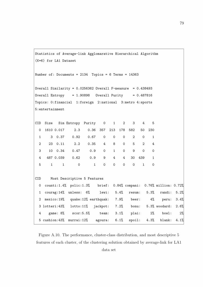
79

Statistics of Average-link Agglomarative Hierarchical Algorithm

(K=6) for LA1 Dataset





5:entertainment


0 1610 0.017 2.3 0.36 357 213 178 582 50 230

1 3 0.37 0.92 0.67 0 0 0 2 0 1

2 23 0.11 2.2 0.35 4 8 0 5 2 4

3 10 0.34 0.47 0.9 0 1 0 9 0 0

4 487 0.039 0.62 0.9 9 4 4 30 439 1

5 1 1 0 1 0 0 0 0 1 0


0 counti:1.4% polic:1.3% brief: 0.84% compani: 0.76% million: 0.72%

1 courag:14% unless: 6% lewi: 5.4% resum: 5.3% randi: 5.2%

2 mexico:19% quake:12% earthquak: 7.9% beer: 4% peru: 3.4%

3 lotteri:43% lotto:11% jackpot: 7.2% bonu: 5.3% woodard: 2.6%

4 game: 8% scor:5.5% team: 3.1% plai: 2% bowl: 2%

5 cushion:43% murrai:12% agoura: 6.1% spoil: 4.3% blank: 4.1%


features of each cluster, of the clustering solution obtained by average-link for LA1

data set

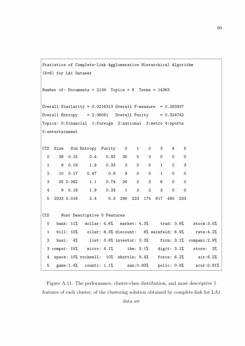
80

Statistics of Complete-link Agglomerative Hierarchical Algorithm






5:entertainment


0 38 0.15 0.4 0.92 35 0 3 0 0 0

1 9 0.19 1.9 0.33 3 0 0 1 2 3

2 10 0.17 0.47 0.9 9 0 0 1 0 0

3 35 0.082 1.1 0.74 26 0 3 6 0 0

4 9 0.18 1.9 0.33 1 3 2 3 0 0

5 2033 0.016 2.4 0.3 296 223 174 617 490 233


0 bank: 11% dollar: 4.6% market: 4.3% trad: 3.9% stock:3.5%

1 bill: 10% oiler: 8.3% discount: 8% seinfeld: 6.9% rate:4.2%

2 busi: 4% list: 3.6% investor: 3.3% firm: 3.1% compani:2.9%

3 comput: 15% micro: 4.1% ibm: 3.1% digit: 3.1% store: 3%

4 space: 10% rockwell: 10% shuttle: 9.4% force: 6.2% air:6.2%

5 game:1.4% counti: 1.1% san:0.93% polic: 0.9% scor:0.81%


features of each cluster, of the clustering solution obtained by complete-link for LA1

data set

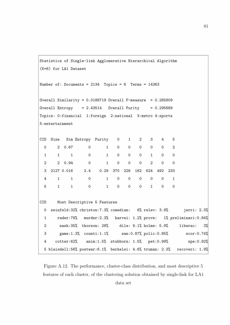
81

Statistics of Single-link Agglomerative Hierarchical Algorithm






5:entertainment


0 2 0.67 0 1 0 0 0 0 0 2

1 1 1 0 1 0 0 0 1 0 0

2 2 0.94 0 1 0 0 0 2 0 0

3 2127 0.016 2.4 0.29 370 226 182 624 492 233

4 1 1 0 1 0 0 0 0 0 1

5 1 1 0 1 0 0 0 1 0 0


0 seinfeld:32% christon:7.3% comedian: 6% relev: 3.9% jerri: 2.3%

1 rader:78% murder:2.3% harvei: 1.2% prove: 1% preliminari:0.84%

2 nash:35% thorson: 28% dile: 9.1% holme: 5.9% liberac: 3%

3 game:1.3% counti:1.1% san:0.87% polic:0.85% scor:0.74%

4 cotter:62% anim:1.5% stubborn: 1.5% pet:0.99% spe:0.92%

5 blaisdell:56% postwar:6.1% berkelei: 4.6% truman: 2.3% recoveri: 1.9%


features of each cluster, of the clustering solution obtained by single-link for LA1

data set

82

Statistics of K-means Algorithm (K=10) for Reuters-21578 Dataset




CID Size Sim Entropy Purity MPT # of Docs from MPT

0 506 0.057 3.7 0.65 crude 328

1 1464 0.19 0.03 1 earn 1461

2 753 0.38 4 0.2 acq 150

3 797 0.084 0.4 0.019 earn 15

4 642 0.13 0.017 1 earn 641

5 552 0.1 2.3 0.43 interest 237

6 1058 0.059 5 0.27 trade 287

7 2210 0.02 1.6 0.62 acq 1365

8 859 0.047 2.8 0.1 coffee 88

9 762 0.055 6.6 0.49 grain 373


0 oil:34% barrel:5.9% crude: 4% opec: 2.6% price: 2.4%

1 loss:23% net:18% shr: 16% mln: 8% rev: 7.9%

2 blah:97% fed:0.21% billion: 0.15% dlr: 0.1% bank:0.076%

3 bond:13% issu:13% debentur: 4.5% manag: 4.3% coupon: 3.1%

4 div:17% qtly:16% record: 14% dividend: 9.5% prior: 9.1%

5 stg:20% bank:11% rate: 6.9% bill: 6.3% monei: 5.6%

6 billion:9.1% trade:5.1% januari: 5% februari: 4.8% dollar: 3.3%

7 share:8.2% compani:3.8% dlr: 2.7% offer: 2.6% stock: 2.3%

8 bank:12% debt:11% loan: 4.9% brazil: 4.1% coffe: 2.3%

9 tonn:28% wheat:7.5% sugar: 4.5% export: 3.6% grain: 3.1%


features of each cluster, of the clustering solution obtained by k-means for

Reuters-21578 data set

83

Statistics of Bisecting K-means Algorithm (K=10) for Reuters-21578

Dataset





0 506 0.057 3.7 0.65 crude 328

1 1464 0.19 0.03 1 earn 1461

2 753 0.38 4 0.2 acq 150

3 797 0.084 0.4 0.019 earn 15

4 642 0.13 0.017 1 earn 641

5 552 0.1 2.3 0.43 interest 237

6 1058 0.059 5 0.27 trade 287

7 2210 0.02 1.6 0.62 acq 1365

8 859 0.047 2.8 0.1 coffee 88

9 762 0.055 6.6 0.49 grain 373


0 oil:34% barrel:5.9% crude:4% opec:2.6% price:2.4%

1 loss:23% net:18% shr:16% mln:8% rev: 7.9%

2 blah:97% fed:0.21% billion:0.15% dlr:0.1% bank:0.076%

3 bond:13% issu:13% debentur:4.5% manag:4.3% coupon:3.1%

4 div:17% qtly:16% record:14% dividend:9.5% prior:9.1%

5 stg:20% bank:11% rate:6.9% bill:6.3% monei:5.6%

6 billion:9.1% trade:5.1% januari:5% februari:4.8% dollar:3.3%

7 share:8.2% compani:3.8% dlr:2.7% offer:2.6% stock:2.3%

8 bank:12% debt:11% loan:4.9% brazil:4.1% coffe:2.3%

9 tonn:28% wheat:7.5% sugar:4.5% export:3.6% grain:3.1%




84

Statistics of Divisive Hierarchical Algorithm (K=10) for

Reuters-21578 Dataset





0 1457 0.026 6.1 0.16 grain 237

1 1366 0.14 2.8 0.55 earn 750

2 2620 0.034 5.2 0.16 money-fx 429

3 1555 0.033 1.2 0.4 acq 621

4 1667 0.16 0.18 0.97 earn 1621

5 59 0.058 2.4 0.58 ship 34

6 428 0.024 1.2 0.65 acq 280

7 309 0.033 0.91 0.69 acq 214

8 108 0.094 4 0.46 gold 50

9 34 0.12 3 0.38 ship 13


0 tonn: 7.8% oil: 3.4% export: 2.7% wheat: 2.2% price: 1.7%

1 blah: 77% qtly: 3.2% div: 3.1% record: 2.7% dividend: 1.8%

2 bank: 8.7% billion: 5.2% rate: 2.8% trade: 1.9% stg: 1.8%

3 issu: 5.6% offer: 5.6% bond: 4.2% share: 3.8% debentur: 3.4%

4 loss: 23% net: 18% shr: 15% mln: 8.5% rev: 7.4%

5 ship: 17% portland: 7.7% port: 7.3% load: 4.2% coastal: 3.9%

6 sale: 4% complet: 3.8% unit: 3.2% compani: 3% acquisit: 2.9%

7 share: 11% usair: 5.3% merger: 4.8% compani: 3.8% earn: 3.1%

8 mine: 23% gold: 19% ounc: 7.2% grade: 4.4% ton: 3.9%

9 strike: 23% seamen: 11% union: 6.4% port: 2.7% marin: 2.6%



clustering for Reuters-21578 data set

85

Statistics of Average-link Algorithm (K=10) for Reuters-21578





0 9085 0.024 4 0.31 earn 2839

1 222 0.064 3.5 0.36 gold 79

2 2 0.73 0 1 acq 2

3 4 0.59 0 1 acq 4

4 16 0.12 0.72 0.56 acq 9

5 216 0.047 2.7 0.63 ship 135

6 33 0.1 2.1 0.3 acq 10

7 20 0.12 1.5 0.45 acq 9

8 3 0.58 0.39 0.67 acq 2

9 2 0.64 0 1 acq 2


0 blah: 10% loss: 5.7% mln: 5.2% net: 4.5% shr: 3.7%

1 gold: 17% mine: 16% ounc: 8.5% ton: 7.7% copper: 6.6%

2 gerber: 65% gst: 8% cwt: 6.8% buyout: 3% fremont: 2.3%

3 gate: 46% learjet: 22% interconnect:14% norri: 5.6% berri: 3.9%

4 print: 12% magazin: 9.4% newspap: 8.3% southam: 5.7% printer: 5.3%

5 ship: 12% strike: 7.7% gulf: 5.3% port: 4.7% seamen: 3.2%

6 coastal:17% court:8.3% transamerican:6.6% suffield:6.3% bankruptci: 4.2%

7 arco: 7.8% ciba: 7.1% cell: 5.8% sandoz: 5.6% quest: 4.4%

8 imatron: 45% mitsui: 29% benigno: 3.8% kidnap: 3.5% businessman:2.2%

9 saatchi: 55% jwt: 25% cleveland: 4.1% advertis: 2.5% ted: 2.2%


features of each cluster, of the clustering solution obtained by average-link for


86

Statistics of Complete-link Algorithm (K=10) for Reuters-21578





0 90 0.23 0.88 0.92 coffee 83

1 37 0.16 3.8 0.97 grain 36

2 66 0.24 2.9 1 grain 66

3 21 0.11 3.9 0.43 crude 9

4 6 0.53 1.3 0.67 acq 4

5 10 0.3 0.88 0.7 acq 7

6 345 0.23 0 1 earn 345

7 28 0.093 1.2 0.5 acq 14

8 478 0.4 0 1 earn 478

9 8522 0.021 4.2 0.24 earn 2039


0 coffe:46% quota: 8.1% ico: 7.6% bag: 4.2% export: 3.9%

1 grain:44% load: 6.9% portland: 6.1% ship: 2.9% gulf: 2.8%

2 wheat:49% tonn: 22% export: 1.9% soviet: 1.5% depart: 1.1%

3 usx:9.1% tax: 7.1% field: 4.5% roderick: 4% hog:3.8%

4 champion:73% claremont: 7.6% echlin: 2.1% blah: 1.1% board: 1%

5 comput:55% microfilm: 8.9% wavehil: 4.3% comi: 2.8% person:2.5%

6 net 29% shr: 24% mln: 12% rev: 10% qtr: 5.3%

7 seali:7.8% ohio: 5.9% triton: 5.2% mln: 3.9% neoax:3.9%

8 loss:59% profit: 14% shr: 6.5% net: 5.5% rev: 4.3%

9 blah:14% mln: 3.2% bank: 2.8% dlr: 2.2% billion: 2.2%




87

Statistics of Single-link Algorithm (K=10) for Reuters-21578





0 1 1 0 1 acq 1

1 1 1 0 1 acq 1

2 1 1 0 1 acq 1

3 1 1 0 1 acq 1

4 1 1 0 1 acq 1

5 1 1 0 1 acq 1

6 1 1 0 1 pet-chem 1

7 1 1 0 1 acq 1

8 9594 0.023 4.1 0.3 earn 2876

9 1 1 0 1 earn 1


0 amsouth:65% tuskaloosa: 10% affili: 10% aso: 2.6% approv: 2.2%

1 mcfarland:88% approv: 1.3% santa: 1.2% spring: 1.1% exchang:0.89%

2 avia:66% reebok: 14% stockhold: 3.6% portland: 1.5% complaint:1.4%

3 dumez:65% westburn: 23% unicorp: 1.7% share: 1% common:0.94%

4 lazer:42% fidelcor: 38% ficr: 2.4% acquir: 2% bkne: 1.8%

5 seton:82% sel: 2.3% newark: 1.4% member: 1.3% chairman: 1%

6 protocol:15% aerosol: 9.1% layer: 7.7% scientist: 6.7% earth:6.4%

7 frick:44% frigid: 25% coil: 8.9% refriger: 7.4% compressor:2.5%

8 blah:10% loss: 5.5% mln: 5.1% net: 4.3% shr: 3.6%

9 ncr:67% proced: 2.2% major: 1.6% strongest: 1.6% deliver:1.4%


features of each cluster, of the clustering solution obtained by single-link for


88

Statistics of K-Means Algorithm (K=10) for Wap Dataset





0 191 0.068 2.9 0.27 business 52

1 97 0.075 0.56 0.92 sports 89

2 461 0.035 2.5 0.39 film 180

3 96 0.1 1.6 0.64 politics 61

4 193 0.049 2.5 0.43 music 83

5 71 0.12 0 1 health 71

6 140 0.053 2.6 0.49 people 69

7 24 0.18 0 1 health 24

8 245 0.054 0.068 0.99 health 243

9 42 0.17 1.8 0.43 culture 18


0 walter:8.1% gail: 4.3% militari: 3.2% liquor: 2.8% loan: 2.6%

1 diaz:11% neurosurgeri: 2.1% mira: 1.7% agnieszka: 1.7% vehicl:1.6%

2 elit:5.5% craig: 1.8% degen: 1.4% uncompl: 1.3% chiffon: 1.3%

3 thrive:11% virsa: 7% construct: 5.6% trevor: 4.2% duplic: 3.3%

4 academi:5.1% dar: 3.4% slovakia: 2.8% cathol: 2.4% arbitr: 1.9%

5 hornbi:26% marshal: 4.7% incen: 3.4% bess: 3% sheila: 2.3%

6 evidenc:12% neonat: 3.4% widescreen: 2.9% statem: 2.5% backward:2.1%

7 kendrick:10% lesson: 8.6% fetch: 5.8% rees: 5.6% suspicion: 4.4%

8 grammi:4.6% nato: 4.1% confidentia: 3.6% jude: 3.4% toll: 2.7%

9 plant: 11% restag: 9.4% sofa: 6.7% edinburgh: 5.8% lousi: 5.1%


features of each cluster, of the clustering solution obtained by k-means for Wap data

set

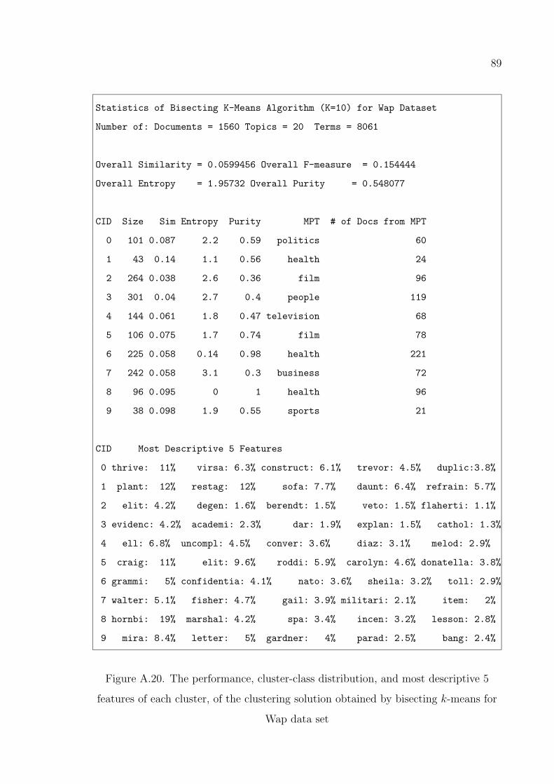
89

Statistics of Bisecting K-Means Algorithm (K=10) for Wap Dataset





0 101 0.087 2.2 0.59 politics 60

1 43 0.14 1.1 0.56 health 24

2 264 0.038 2.6 0.36 film 96

3 301 0.04 2.7 0.4 people 119

4 144 0.061 1.8 0.47 television 68

5 106 0.075 1.7 0.74 film 78

6 225 0.058 0.14 0.98 health 221

7 242 0.058 3.1 0.3 business 72

8 96 0.095 0 1 health 96

9 38 0.098 1.9 0.55 sports 21


0 thrive: 11% virsa: 6.3% construct: 6.1% trevor: 4.5% duplic:3.8%

1 plant: 12% restag: 12% sofa: 7.7% daunt: 6.4% refrain: 5.7%

2 elit: 4.2% degen: 1.6% berendt: 1.5% veto: 1.5% flaherti: 1.1%

3 evidenc: 4.2% academi: 2.3% dar: 1.9% explan: 1.5% cathol: 1.3%

4 ell: 6.8% uncompl: 4.5% conver: 3.6% diaz: 3.1% melod: 2.9%

5 craig: 11% elit: 9.6% roddi: 5.9% carolyn: 4.6% donatella: 3.8%

6 grammi: 5% confidentia: 4.1% nato: 3.6% sheila: 3.2% toll: 2.9%

7 walter: 5.1% fisher: 4.7% gail: 3.9% militari: 2.1% item: 2%

8 hornbi: 19% marshal: 4.2% spa: 3.4% incen: 3.2% lesson: 2.8%

9 mira: 8.4% letter: 5% gardner: 4% parad: 2.5% bang: 2.4%



Wap data set

90

Statistics of Divisive Hierarchical Algorithm (K=10) for WAP





0 9 0.24 2.1 0.44 art 4

1 43 0.073 3 0.28 music 12

2 796 0.027 3.2 0.19 film 151

3 69 0.11 1.9 0.52 technology 36

4 618 0.031 2.4 0.55 health 338

5 10 0.18 1.3 0.6 culture 6

6 2 0.97 0 1 film 2

7 2 0.68 0 1 people 2

8 2 0.54 0 1 cable 2

9 9 0.26 2.2 0.33 film 3


0 recollect:11% ethan:6.1% georgetown: 4.2% chelsea:3.8% kafelnikov: 2.3%

1 incid:5.5% libel: 5.4% slovakia: 4.9% bang: 4.6% rowan: 3%

2 elit:3.1% degen: 1.1% evidenc: 1% restag: 0.92% ell:0.84%

3 walter:14% militari: 5.9% loan: 4.9% shuttl: 3% gail:2.7%

4 nato: 2% confidentia: 1.9% hornbi: 1.9% grammi: 1.7% marshal:1.7%

5 portabl:15% omar: 8.2% subsid: 6.1% buena: 2.9% budget: 2.6%

6 psychiatr:46% jesper: 16% marijuana: 5% elit: 2% dad: 1.6%

7 lousi:9.6% mckinlei: 5.9% nathan: 5.8% feloni: 5.5% nchant:4.9%

8 decor:9.6% prostat: 7.2% distort: 5.8% moonlight: 3.8% meer:2.7%

9 specter:34% exacerb: 9.6% paxson: 3.6% vaccin: 2% steam: 2%



clustering for Wap data set

91

Statistics of Average-link Algorithm (K=10) for Wap Dataset





0 699 0.031 3.1 0.24 film 168

1 12 0.22 2 0.5 culture 6

2 8 0.25 1.6 0.38 film 3

3 36 0.19 2.3 0.5 culture 18

4 5 0.25 0.72 0.8 review 4

5 12 0.18 2 0.5 film 6

6 326 0.054 0.2 0.98 health 319

7 9 0.3 2.1 0.44 multimedia 4

8 349 0.043 3.5 0.21 business 73

9 104 0.076 0.43 0.93 sports 97


0 elit: 4.1% evidenc: 1.3% craig: 1.1% moonlight: 1.1% degen: 1.1%

1 bang: 15% game: 14% libel: 10% incid: 6.3% wallac: 5.3%

2 mccourt:14% masterpiec: 11% tycoon: 6.6% macdonald: 6.3% transport: 6.1%

3 restag: 16% plant: 13% sofa: 8.3% refrain: 5.9% argum: 5.6%

4 headquart: 8.8% featur: 7.1% elisabeth: 5.8% diva: 5.5% braill: 4.2%

5 fbi: 8.4% andrea: 8.2% gather: 6.7% danni: 6.6% qualiti: 4.7%

6 hornbi: 3.9% confidentia: 3.7% nato: 3.6% grammi: 3.4% marshal: 3.4%

7 orphan: 35% reform: 15% preterm: 12% coffin: 4.7% trash: 4.6%

8 walter: 3.7% fisher: 2.9% gail: 2.3% thrive: 2% militari: 1.5%

9 diaz: 9.4% edinburgh: 3.3% snub: 2.2% neurosurgeri: 1.9% agnieszka: 1.6%


features of each cluster, of the clustering solution obtained by average-link for Wap

data set

92

Statistics of Complete-link Algorithm (K=10) for Wap Dataset





0 24 0.099 2.2 0.38 music 9

1 15 0.18 2.3 0.4 culture 6

2 13 0.2 0.39 0.92 music 12

3 237 0.059 0.039 1 health 236

4 23 0.098 2.9 0.26 television 6

5 61 0.12 1.4 0.77 television 47

6 10 0.22 2 0.4 people 4

7 20 0.12 2.7 0.4 business 8

8 51 0.17 1.7 0.71 politics 36

9 1106 0.023 3.8 0.17 film 186


0 kurfuerstendam:6% vincent: 5.6% georgetown:3.1% dairi: 3.1% academi:2.1%

1 game: 17% bang: 12% libel: 7.3% incid: 4.2% wallac: 4.2%

2 viral: 13% academi: 9.8% simplifi: 6.6% screwbal: 6.3% robin: 5.8%

3 hornbi: 4.9% nato: 4.2% grammi: 3.8% marshal: 3.6% confidentia: 3.5%

4 amanda: 7.8% haven: 6.6% yugoslav: 5.2% belov: 3.4% slovakia: 2.3%

5 conver: 9.2% melod: 7.7% uncompl: 7.2% unopen: 6.3% pierr: 6%

6 specter: 21% exacerb: 6.7% chemic: 5.3% modern: 4.1% breakthrough:3.5%

7 sporad: 8.8% intern: 6.3% kick: 5.8% henman: 5.8% ordinari: 3.8%

8 thrive: 15% construct: 9.4% virsa: 8.4% trevor: 7.8% duplic: 5.6%

9 elit: 2.2% carolyn:0.85% walter:0.79% gail: 0.7% degen:0.62%


features of each cluster, of the clustering solution obtained by complete-link for Wap

data set

93

Statistics of Single-link Algorithm (K=10) for Wap Dataset





0 1551 0.021 3.7 0.22 health 341

1 1 1 0 1 review 1

2 1 1 0 1 review 1

3 1 1 0 1 review 1

4 1 1 0 1 review 1

5 1 1 0 1 people 1

6 1 1 0 1 review 1

7 1 1 0 1 review 1

8 1 1 0 1 review 1

9 1 1 0 1 review 1


0 elit: 1.5% carolyn:0.65% melod:0.63% restag:0.58% nato:0.53%

1 frazier: 12% agent: 8.3% tandem: 5.2% octob: 4.1% costa: 2.9%

2 highwai: 16% brown: 9.6% encompass: 4.8% undermin: 2.8% produc: 2.7%

3 rental: 8.2% stupid: 3.6% dog: 3.6% appreci: 3.6% jovi: 3.6%

4 barri: 8.8% westport: 6.1% sleep: 4.2% assum: 3.2% enqvist: 3.2%

5 rule: 21% held: 16% elig: 14% judith: 6% exclu: 3.2%

6 talli: 8.4% reiner: 4.1% physiolog: 3.5% entitl: 3.5% rusedski: 3.1%

7 furiou: 14% petrikin: 8.8% morton: 7.2% lar: 4.2% rough: 2.6%

8shutout: 22% wareh: 18% buck: 5.5% pen: 2.9% stumbl: 2.1%

9 basqu: 11% blunt: 6.7% light: 5.3% illumin: 3.9% garri: 3.7%


features of each cluster, of the clustering solution obtained by single-link for Wap

data set

94

REFERENCES

1. Sebastiani, F., “Machine Learning in Automated Text Categorization”, ACM Com-

puting Surveys , Vol. 34, No. 1, pp. 1–47, 2002.

2. Masand, B., G. Linoff, and D. Waltz, “Classifying News Stories Using Memory

Based Reasoning”, 15th Ann Int ACM SIGIR Conference on Research and Devel-

opment in Information Retrieval , pp. 59–64, 1992.

3. Yang, Y., “An Evaluation of Statistical Approaches to Text Categorization”, Jour-

nal of Information Retrieval , Vol. 1, No. 1–2, pp. 69–90, 1999.

4. Yang, Y. and J. P. Pedersen, “A Comperative Study on Feature Selection in Text

Categorization”, The Fourteenth International Conference on Machine Learning ,

pp. 412–420, 1997.

5. Joachims, T., “Text Categorization with Support Vector Machines: Learning with

Many Relevant Features”, European Conference on Machine Learning (ECML),

1998.

6. Ng, H. T., W. B. Goh, and K. L. Low, “Feature Selection, Perceptron Learning,

and a Usability Case Study for Text Categorization”, 20th Ann Int ACM SIGIR

Conference on Research and Development in Information Retrieval , pp. 67–73,

1997.

7. Wiener, E., J. O. Pedersen, and A. S. Weigend, “A Neural Network Approach

to Topic Spotting”, Proceedings of the Fourth Annual Symposium on Document

Analysis and Information Retrieval , 1995.

8. Yang, Y. and X. Liu, “A Re-examination of Text Categorization Methods”, Pro-

ceedings of SIGIR-99, 22nd ACM International Conference on Research and De-

velopment in Information Retrieval , Berkeley, US, 1999.

95

9. McCallum, A. and K. Nigam, “A Comparison of Event Models for Naive Bayes Text

Classification”, AAAI-98 Workshop on Learning for Text Categorization, 1998.

10. Koller, D. and M. Sahami, “Hierarchically Classifying Documents Using Very Few

Words”, Proceedings of 14th International Conference on Machine Learning , pp.

170–178, Nashville, US, 1997.

11. Larkey, L. S., “A Patent Search and Classification System”, Proceedings of 4th

ACM Conference on Digital Libraries, pp. 179–187, Berkely, US, 1999.

12. Ozgur, L., Adaptive Anti-Spam Filtering Based on Turkish Morphological Anal-

ysis, Artificial Neural Networks and Bayes Filtering , Master’s Thesis, Bogazici

University, Turkey, 2003.

13. Sahami, M., S. Dumais, D. Heckerman, and E. Horvitz, “A Bayesian Approach to

Filtering Junk E-Mail”, Sahami, M., editor, Proceedings of AAAI-98 Workshop on

Learning for Text Categorization, 1998.

14. Dumais, S. T. and H. Chen, “Hierarchical Classification of Web Content”, Pro-

ceedings of SIGIR-00, 23rd ACM International Conference on Research and De-

velopment in Information Retrieval , pp. 256–263, Athens, GR, 2000.

15. Zamir, O., O. Etzioni, O. Madani, and R. M. Karp, “Fast and Intuitive Clustering

of Web Documents”, KDD’97 , pp. 287–290, 1997.

16. Jain, A. K., M. N. Murty, and P. J. Flynn, “Data Clustering: A Review”, ACM

Computing Surveys, Vol. 31, No. 3, pp. 264–323, September 1999.

17. Zhao, Y. and G. Karypis, “Evaluation of Hierarchical Clustering Algorithms for

Document Datasets”, Proceedings of CIKM , 2002.

18. Steinbach, M., G. Karypis, and V. Kumar, “A Comparison of Document Clustering

Techniques”, KDD Workshop on Text Mining , 1999.

96

19. Salton, G., C. Yang, and A. Wong, “A Vector-Space Model for Automatic Index-

ing”, Communications of the ACM , Vol. 18, No. 11, pp. 613–620, 1975.

20. Cohen, W. W. and Y. Singer, “Context-Sensitive Learning Methods for Text Cat-

egorization”, Proceedings of the 19th Annual ACM SIGIR Conference, 1996.

21. Fuernkranz, J., T. Mitchell, and E. Riloff, “A Case Study in Using Linguistic

Phrases for Text Categorization on the WWW”, Sahami, M., editor, In Learning

for Text Categorization: Papers from the 1998 AAAI Workshop (Technical Report

WS-98-05), 1998.

22. Dumais, S., T. Platt, D. Heckermann, and M. Sahami, “Inductive Learning Algo-

rithms and Representations for Text Categorization”, Proceedings of the Seventh

International Conference on Information and Knowledge Management , 1998.

23. Sahami, M., Using Machine Learning To Improve Information Access, Ph.D. The-

sis, Stanford University, 1998.

24. Porter, M. F., “An Algorithm for Suffix Stripping”, Program, Vol. 14, pp. 130–137,

1980.

25. ftp://ftp.cs.cornell.edu/pub/smart/, 2004.

26. http://www.tartarus.org/ martin/PorterStemmer/, 2004.

27. Aas, L. and L. Eikvil, “Text Categorisation: A Survey”, 941, Norwegian Comput-

ing Center, June 1999.

28. Salton, G. and C. Buckley, “Term Weighting Approaches in Automatic Text Re-

trieval”, Information Processing and Management , Vol. 24, No. 5, pp. 513–523,

1988.

29. Manning, C. D. and H. Schutze, Foundations of Statistical Natural Language Pro-

cessing , The MIT Press, Cambridge, Massachusetts, USA, 1999.

97

30. Cohen, Empirical Methods in AI , MIT Press, 1999.

31. Spitters, M., “Comparing Feature Sets for Learning Text Categorization”, Proceed-

ings of RIAO 2000 , April 2000.

32. Hartigan, J., Clustering Algorithms, John Wiley & Sons, New York, NY, 1975.

33. Berkhin, P., “Survey of Clustering Data Mining Techniques”, Research paper,

Accrue Software, http://www.accrue.com/products/researchpapers.html, 2002.

34. Forgy, E., “Cluster Analysis of Multivariate Data: Efficiency Versus Interpretabil-

ity of Classification”, Biometrics , Vol. 21, pp. 768–780, 1965.

35. Kaufman, L. and P. Rousseeuw, Finding Groups in Data, Wiley, New York, NY,

1990.

36. Mitchell, T. M., Machine Learning , McGraw Hill, 1997.

37. Joachims, T., “A Probabilistic Analysis of the Rocchio Algorithm with TFIDF for

Text Categorization”, ICML-97 , 1997.

38. Burges, C. J. C., “A Tutorial on Support Vector Machines for Pattern Recogni-

tion”, Data Mining and Knowledge Discovery , Vol. 2, No. 2, pp. 121–167, 1998.

39. Joachims, T., “Making Large-Scale SVM Learning Practical”, Report LS-8, Uni-

versitat Dortmund, 1998.

40. Joachims, T., Advances in Kernel Methods-Support Vector Learning , chapter Mak-

ing Large-Scale SVM Learning Practical, MIT-Press, 1999.

41. “TREC. Text Retrieval Conference”, http://trec.nist.gov, 1999.

42. Lewis, D. D., “Reuters-21578 Document Corpus V1.0”, http://kdd.ics.uci.edu

/databases/reuters21578/reuters21578.html, 2004.

98

43. Han, E.-H. S., D. Boley, M. Gini, R. Gross, K. Hastings, G. Karypis, V. Kumar,

B. Mobasher, and J. Moore, “Webace: A Web Agent for Document Categorization

and Exploration”, Proceedings of the 2nd International Conference on Autonomous

Agents , 1998.

44. Karypis, G., “Cluto 2.0 Clustering Toolkit”, http://www.users.cs.umn.edu

/∼karypis/cluto, 2004.

45. van Rijsbergen, C. J., Information Retrieval , Butterworths, London, 1979.

SUPERVISED AND UNSUPERVISED MACHINE LEARNING TECHNIQUES FOR TEXT...

Documents

Transcript of SUPERVISED AND UNSUPERVISED MACHINE LEARNING TECHNIQUES FOR TEXT...