Supermarkets, farm household income and poverty:

Insights from Kenya

By

Rao, Elizaphan J.O. and Qaim, Matin

Contributed Paper presented at the Joint 3rd African Association of Agricultural

Economists (AAAE) and 48th Agricultural Economists Association of South Africa

(AEASA) Conference, Cape Town, South Africa, September 19-23, 2010.

1

Supermarkets, farm household income and poverty: Insights from Kenya1

Elizaphan J.O. Rao and Matin Qaim

Department of Agricultural Economics and Rural Development Georg-August-University of Goettingen

37073 Goettingen, Germany

January 2010

                                                            1 This research was financially supported through a grant from the German Research Foundation (DFG).

2

Abstract

Expansion of supermarkets in developing countries is increasingly providing opportunities for

farmers to participate in modern supply chains. While some farmers are excluded by stringent

supermarket requirements, there are important gains for participating farmers. However, studies

analyzing income effects of high-value chains use approaches that either show no causality or

ignore structural differences between farmers in different channels. Using endogenous switching

regression and data from a survey of vegetable growers in Kenya, we account for systematic

differences and show that participation in supermarket chains yields 50% gain in household

income leading to 33% reduction in poverty. Supermarket expansion is therefore likely to have

substantial welfare effects if more farmers are supported to overcome inherent entry barriers.

Keywords: supermarkets, per capita income, sample selection, endogenous switching

regression, Kenya, Africa

1. Introduction

Increasing demand for high-value food products in developing countries is creating incentives

for expansion of supermarkets (Neven et al., 2006; Reardon et al., 2003). And in order to meet

arising consumer concerns, emerging supermarkets increasingly adopt tighter vertical

coordination involving direct procurement from farmers. These changes have crucial

implications for farm households. While there is potential for exclusion of some farmers due to

stringent requirements imposed by supermarkets, there are also potential welfare gains for

3

farmers who have access to these channels. Stable prices and contractual arrangements offered

by supermarkets for instance, improve income flows for farmers in supermarket channels.

Expansion of supermarkets in developing countries can therefore have substantial effects on farm

household income and on rural poverty in general.

In light of these changes, there is a growing body of literature analyzing implications of

supermarket expansion for rural households (Neven and Reardon, 2004; Pingali et al., 2007;

Reardon et al., 2009). Most studies focus on determinants of participation in supermarket

channels and institutional innovations for integrating farmers into these modern supply chains

(Hernandez et al., 2007; Moustier et al., 2009; Neven et al., 2009). Some studies also evaluate

welfare effects of emerging supermarket chains in developing countries. However, current

studies on welfare effects employ gross margin analysis (Hernandez et al., 2007; Neven et al.,

2009) that do not reveal causality. While there may be significant differences in gross margins

across market channels, such differences cannot be attributed to participation in supermarket

chains without analytical procedures that show causality.

On the other hand there are also studies on the welfare effects of global supply chains (Bolwig et

al., 2009; Maertens and Swinnen, 2009; Minten et al., 2009; Miyata et al., 2009; Warning and

Key, 2002; Wollni and Zeller, 2007). These global chains involve contracting of farmers in

developing countries for export markets and the respective studies use standard treatment effect

models to measure welfare effects while accounting for sample selection. However, the treatment

models assume uniform effect across groups of observations. Yet evidence from recent studies

show systematic differences between farmers supplying supermarkets and their counterparts in

traditional channels (Hernandez et al., 2007; Neven et al., 2009). Welfare measures such as

4

income are therefore likely to differ structurally, depending on the market channels, especially if

participation in supermarket channels is also associated with the factors that affect income.

If income functions indeed differ across market channels, then assuming uniform effect conceals

inherent interaction between channel adoption and other factors influencing income. This can

lead to inappropriate policy recommendation. Furthermore, understanding how factors affecting

income interact with decision to participate in supermarket channels is also crucial, particularly

in developing innovations aimed at enhancing famer participation in these channels.

In this paper, we analyze income effects of participation in supermarket chains using more

efficient correction for sample selection. We use a switching regression model that treats market

channels as regimes and thus allows for structural differences in income functions of farmers

across market channels. And to account for some unobserved factors that jointly influence

household income and choice of market channel, we use an endogenous version of the switching

model. This yields income effects that vary according to market regimes, thus providing more

accurate information that can aid targeting of market access interventions. We hypothesize an

intercept shift in income function due to supermarket participation and an interaction between

the choice of market channel and other factors influencing income.  

Moreover, our approach allows us to simulate potential poverty effects of modern supply chains.

To our knowledge none of the previous studies on welfare effects of supermarket expansion has

analyzed potential effects on household income and poverty. Our study therefore provides

further insights into welfare effects of modern supply chain and yields more accurate information

for targeted welfare intervention. The study builds on primary data from a survey of vegetable

farmers in Kiambu district of Central Kenya. Supermarkets have been expanding rapidly in

5

Kenya and are already venturing into sales of Fresh Fruits and Vegetables (FFV) (Neven and

Reardon, 2004). Given the role of horticulture in the Kenyan economy, continued expansion of

supermarket channels into FFV sales is therefore likely to have substantial welfare effects for

farm households. 

The paper proceeds as follows. In the next section we present the analytical framework and

estimation procedure for our study. In section three we describe the data and undertake some

descriptive analysis. This is followed by section four where we present and discuss results of our

estimation. Section five concludes the study.

2. Analytical framework and estimation procedures

Participation in supermarket chains can be viewed as a binary choice resulting from

maximization of utility or returns. Utility is in turn determined by a set of exogenous variables Z,

which influence the cost of adjusting to a market option with new requirements. Variables in Z

also determine the relative returns that a farmer can earn from supermarket and spot market

channels. These variables can therefore include farm or household characteristics, asset

ownership and human capital such as education that determine the cost of adjusting to

requirements of a new market.

In choosing market options, farmers therefore compare expected utility of participation in

supermarket chains against utility of participating in traditional markets and supermarket

channel is chosen if . However, and are latent and what is observed is participation

in supermarket chains where if and if . Participation in supermarket

chains can therefore be represented as follows;

(1)

6

where is a vector of parameters and is an error term with zero mean and variance . Since

farmers are heterogeneous in their characteristics, not all farmers will overcome the adjustment

costs to be able to supply in supermarket chains. Nevertheless, participation in supermarkets

often yield returns that can positively affect household income. This could be due to better and

stable prices and steady flow of revenues due to market assurance.

2.1. Modeling income effects

The resulting income effects can be estimated using the following model:

(2)

where is income; is farm and household characteristics known to be affecting household

income; and is a dummy variable for participation in supermarket chains. However, income

response to supermarket participation can originate from two sources. First, differences may

arise purely due to characteristic differences in market channels, even if farmers do not differ in

characteristics. Stable prices and market assurance by supermarkets could lead to improved and

continuous flow of revenues as opposed to fluctuations that are a general characteristic of spot

markets.

Secondly, if participation in supermarket chains is associated with farmer characteristics, then we

would still observe differences in income between market channels. However, due to the self-

selection, this difference cannot be wholly attributed to differences in market channels. The

dummy (I) in equation (2) would therefore provide a bias estimate for income effect of

supermarket participation. Heckman selection-correction model corrects for the self-selection but

assumes uniform effects across market channels. This can still lead to bias estimates if there are

systematic differences across groups of farmers in different market channels. Maertens and

7

Swinnen (2009) use an alternative approach based on propensity score matching. However,

propensity score matching controls for selection on observables and may still yield bias estimates

if hidden bias is substantial. A more suitable approach that corrects for self-selection and

accounts for systematic differences across groups of households is a switching model (Maddala,

1983). The model treats market channels as regime shifters and can be represented as follows:

        

        

(3)

where and represents household income for supermarket and traditional channel suppliers

respectively while is a latent variable determining which regime applies. and are sets of

parameters to be estimated and the variable sets and are allowed to overlap. Note that and

are only partially observed - is only observed for the sample belonging to supermarket

regime and for the sample belonging to traditional channels. So what is totally observed is a

single variable defined as follows:

(4)

From (3), and are residuals that are only contemporaneously correlated and are assumed

to be jointly normally distributed with a mean vector 0, and covariance matrix as follows:

(5)

8

where , , , , , and

. The variance of v is set to one since is estimable only up to a scale factor

(Greene, 2008; Maddala, 1986). In addition since and are never observed together

(Dutoit, 2007).

The switching model so far outlined only accounts for self-selection on observed factors. Yet

there could be unmeasured factors that jointly determine participation in supermarket chains and

household income. Better management skills and entrepreneurial ability can for instance lead to

higher farm/household income. These innate abilities can also influence decision to participate in

supermarket channels. Furthermore, income status may influence supermarket participation by

enhancing farmers’ ability to invest in equipment necessary for participation in supermarket

chains. This implies correlation between the error terms of regime equations and the error term

in selection equation and hence the need for endogenous switching regression model.

Estimates of the covariance terms can therefore provide a test for endogeneity. If

then we have an exogenous switching and if either or is non-zero, then we have a model

with endogenous switching (Maddala, 1986). The test is achieved by testing for significance of

correlation coefficient computed as and (Lokshin and Sajaia,

2004). Assuming these correlations, the expected values of truncated error terms can be

expressed as follows;

(6)

(7)

9

where and are probability density and cumulative distribution of the standard normal

distribution respectively. and are the ratios of and evaluated at - Inverse Mills

Ratios (IMR) (Greene, 2008).

Besides providing a test for endogeneity, the signs of correlation coefficients and have

economic interpretation. If and have alternate signs, then farmers choose supermarket

channels on the basis of their comparative advantage (Fuglie and Bosch, 1995; Maddala, 1983;

Trost, 1981; Willis and Rosen, 1979). Thus, if , then farmers having income above

average income for supermarket suppliers have higher than expected chances of participating in

supermarket channels. Similarly if , then individuals with incomes above average income

of farmers supplying traditional channels have lower than expected chance of supplying

supermarkets. Consequently farmers who supply supermarket channels will have above average

returns from supplying supermarkets. Similarly those who supply traditional channels have

above average returns from supplying traditional channels.

Alternatively when and , then there is evidence of “hierarchical sorting” (Fuglie

and Bosch, 1995; Trost, 1981). In other words, supermarket suppliers have above average returns

whether or not they participate in supermarket channels but are better off in supermarket

channels. Similarly, traditional channel suppliers have below average returns in either case but

are better off supplying traditional channels. Interpretation of the covariance terms also provides

proof for consistency of the model which requires that . This condition also implies

that supermarket suppliers earn higher income than they would earn if they supplied traditional

channels(Trost, 1981).

10

2.2 Estimation procedure

Assuming correlation of the error terms implied in equations (6) and (7), a two-stage method can

be used to estimate the model. The first stage probit model [ ] provides estimates of

which are then used to estimate the IMRs [ and ]. The IMRs are then treated as “missing

variables” in estimating regime equations in (3) by OLS. In order to identify the model we need

to ensure that at least one variable in Z does not appear in X. The coefficients of IMRs would

then provide estimates of covariance terms and . This approach yields consistent but

inefficient estimates of parameters especially if coefficients of and are nonzero (Fuglie and

Bosch, 1995; Trost, 1981). A more efficient approach is the full information maximum

likelihood (FIML) method for endogenous switching regression (Greene, 2008; Lokshin and

Sajaia, 2004). This provides for joint estimation of regime equations and the selection equation.

Note that the coefficients and in equation (3) measure the marginal effects of independent

variables on household income unconditional on farmers actual market choice, i.e. the potential

effect of X on the sample. If there are variables that appear both in X and Z, the coefficients can,

however, be used to estimate conditional effects as follows;

(8)

Equation (7) decomposes effect of change in into two parts: is the direct effect on the

mean of ; the second part is the indirect effect from market choice that appears as a result of

correlation between unobserved component of and I.

2.3. Estimating income effect of supermarket participation

11

In order to evaluate the income effect of participation in supermarket channels, we need to

estimate conditional expectation of income per capita that participants would have without

participation in supermarket channels (Maddala, 1983). This can be estimated, holding other

characteristics constant via the following steps. Assuming a farmer with farm and individual

characteristics (X, Z) who participates in supermarket chains, the expected value of is:

(9)

where the last term takes into account sample selectivity. For the same farm, predicted value of

(expected value of y if the same farm does not participate) is:

(10)

The change in income per capita due to participation in supermarket channels would then be:

(11)

If self-selection is based on comparative advantage, would be greater than zero and

supplying supermarkets will produce greater benefits under self-selection than under random

assignment (Maddala, 1983).

3. Data and descriptive statistics

3.1. Farm survey

Data for this study was collected in 2008 from Kiambu District of Central Province in Kenya.

Kiambu is located in relative proximity to Nairobi and even before the spread of supermarkets it

has been one of the main vegetable-supplying areas for the capital city. Based on information

from the district agricultural office, four of the main vegetable-producing divisions were chosen.

12

In these four divisions, 31 administrative locations were purposively selected, again using

statistical information on vegetable production. Within the locations, vegetable farmers were

sampled randomly. Since farmers that participate in supermarket channels are still the minority,

we oversampled them using complete lists obtained from supermarkets and supermarket traders.

In total, our sample comprises 402 farmers – 133 supermarket suppliers and 269 supplying

vegetables to traditional markets. Using a structured questionnaire, these farmers were

interviewed on vegetable production and marketing details, other farm and non-farm economic

activities, as well as household and contextual characteristics.

Both types of farmers produce vegetables in addition to maize, bananas, and other cash crops.

The main vegetables produced are leafy vegetables, including exotic ones such as spinach and

kale, and indigenous ones such as amaranthus and black nightshade, among others.1

Insert Figure 1 here

Figure 1 shows the different marketing channels for vegetables used by sampled farmers. Some

supermarket suppliers also sell vegetables in traditional spot markets when they have excess

supply. However, for analytical purposes, farmers that supply at least part of their vegetables to

supermarkets are classified as supermarket suppliers.

Spot markets sales are one-off transactions between farmers and retailers or consumers with

neither promise for repeated transactions nor prior agreements on product delivery or price.

Depending on the demand and supply situation, prices are subject to wide fluctuation. Farmers

who are unable to supply directly to wholesale or retail markets sell their produce to spot market

traders who act as intermediaries. Such traders collect vegetables at the farm gate without any

prior agreement. In contrast, supermarkets do have agreements with vegetable farmers regarding

13

product price, physical quality and hygiene, and consistency and regularity in supply (Ngugi et

al., 2007). Price agreements are made before delivery, and prices are relatively stable. Payments

are usually only once a week or every two weeks. All agreements are verbal with no written

contract. Some farmers also supply supermarkets through special traders. Based on similar verbal

agreements, these traders again maintain regular contacts with farmers, in order to be able to

supply supermarkets in a timely and consistent way. Strict supply requirements by supermarkets

have led to specialization among traders. Consequently supermarket traders tend to exclusively

supply modern retail outlets.2

Given the risk of exclusion from emerging modern supply chains for disadvantaged farmers,

there are various organizations in Kenya linking smallholders to supermarket and export

channels. One such organization active in Kiambu is the NGO Farm Concern International

(FCI). FCI trains farmer groups on production of indigenous vegetables before linking them to

various supermarkets in Nairobi (Moore and Raymond, 2006; Ngugi et al., 2007). FCI also

promotes collective action and – through training efforts – helps farmers to meet the strict

delivery standards imposed by supermarkets. Our sample covers 80 vegetable farmers currently

involved in the FCI project in Kiambu District. Out of these, more than half were already

supplying supermarkets at the time of our survey.

3.2. Descriptive analysis

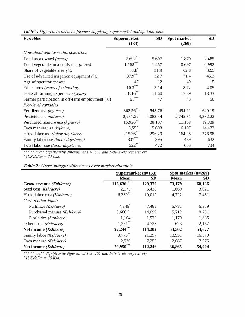
Table 1 shows some descriptive comparison of the two groups of farmers. Farmers in the two

market channels show differences in land ownership, vegetable area cultivated and in the use of

irrigation equipment. They also show differences in education levels and farming experience. On

average, supermarket suppliers own more land and cultivate significantly large area of

vegetables. They also tend to specialize in vegetable production judging from the significant

14

difference in share of vegetable area. Significantly greater proportion of supermarket suppliers

also use advanced irrigation technology, which is seemingly a move to meet supermarket

requirement for consistent supply of vegetables.

Insert Table 1 here

Supermarket suppliers are also significantly younger but have shorter farming experience

compared to spot market suppliers. Significantly larger proportion of supermarket suppliers also

engages in off-farm employment.

Apart from differences in various socioeconomic variables of interest, we carry out economic

analysis of participation in supermarket channels. In Table 2 we present a comparison of gross

margin between farmers in the two market channels.

Insert Table 2 here

The two groups of farmers show significant differences both in revenues and expenditure on

inputs. The differences in revenue is driven both by yields and prices which are higher for

supermarket suppliers. In terms of costs, supermarket suppliers spend significantly more on hired

labour and purchased manure. These higher expenditures reflect higher use of respective inputs

as shown in Table 1. Supermarkets use more labor partly due to extra workforce needed for

packing of vegetables (Neven et al., 2009) and partly due to more regular use of certain inputs

such as purchased manure. This extra demand for hired labor by supermarket suppliers implies

employment creation for rural landless households. Farmers supplying supermarkets, however

use slightly less inorganic fertilizer. Instead, they use more farmyard manure, which they believe

leads to quicker regeneration of leaves after harvest. This is particularly important for

supermarket suppliers that have to supply vegetables more regularly.

15

These differences in revenues and costs result into significantly higher net income per acre for

supermarket suppliers. The picture remains the same even after imputing values for own inputs

such as family labor and own farmyard manure. Unsurprisingly, traditional channel suppliers use

significantly more family labor in vegetable production. These differences in average values of

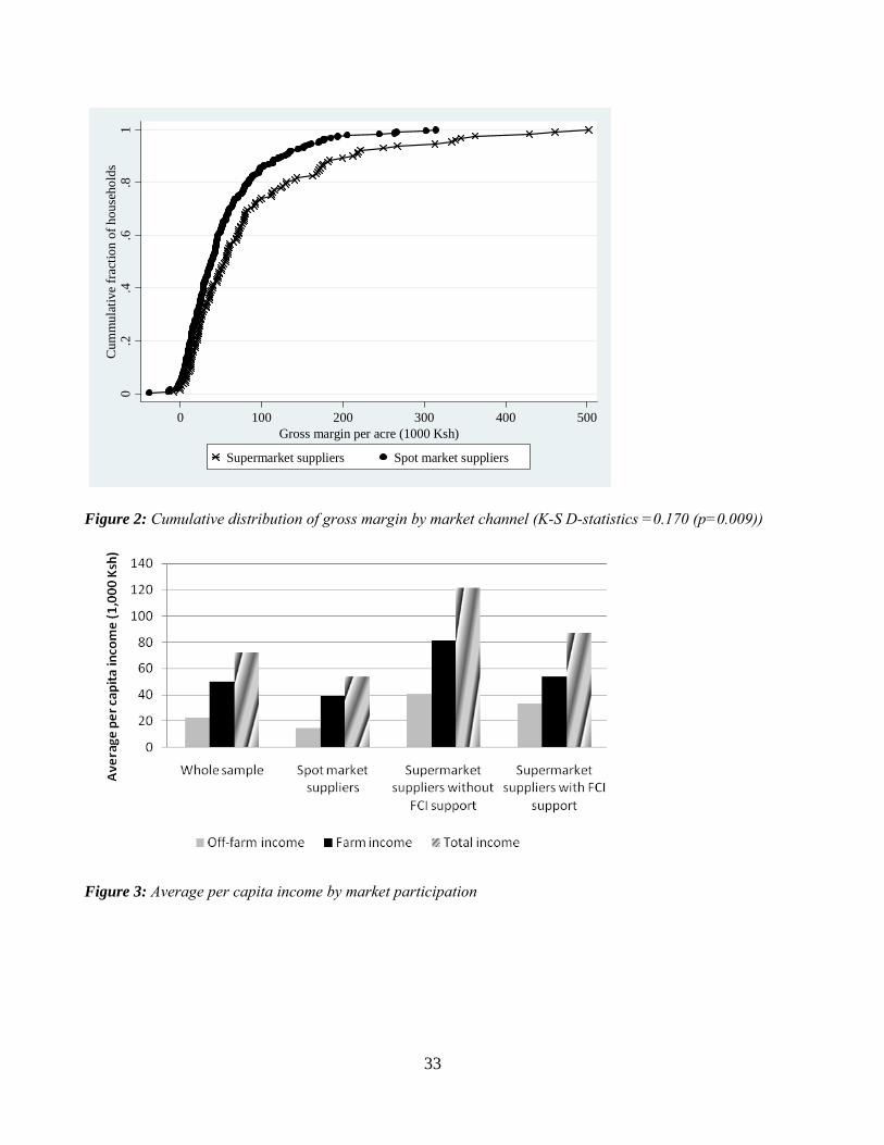
gross margin are replicated across the entire distribution as can be seen from Figure 2. The CDF

of gross margin for supermarket suppliers significantly dominate the CDF for spot market

suppliers.

Insert Figure 2 here

The higher net margin somehow also contributes to higher farm incomes for supermarket

suppliers. However, supermarket suppliers also have higher non-farm income and a combination

of the two income sources yields higher total household income for supermarket suppliers. This

is true both for farmers supplying supermarket on their own as well as for farmers supplying

supermarket via institutional support from FCI. Compared to farmers supplying supermarkets on

their own, FCI-supported farmers are nevertheless inferior in all the income classes. This already

provides an indication of structural differences in household income between supermarket and

traditional channel suppliers.

Insert Figure 3 here

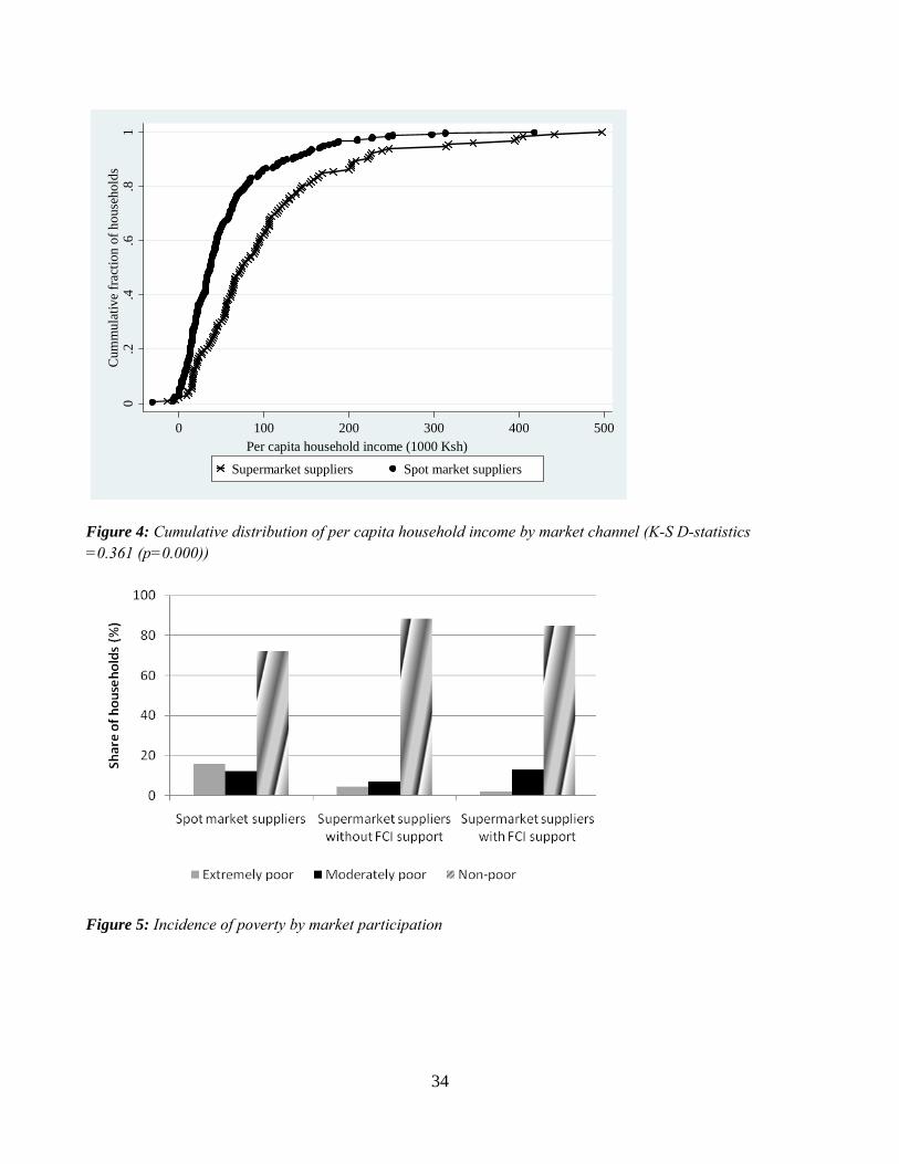
Besides the average values in Figure 3, we also show cumulative distribution of per capita

household income by market channels in Figures 4. The two figures show that supermarket

farmers are significantly superior in both farm and household income nearly across the entire

distribution.

16

Insert Figure 4 here

These superior income distributions translate into lower poverty incidence among supermarket

suppliers as can be seen from Figure 5. Poverty incidences were calculated based on 1.25 dollar

and 2 dollar poverty lines converted to local currency equivalents using purchasing power parity

(PPP) exchange rates. The PPP rates for Kenya was 1 dollar to 29.52 Kenya shillings as at 2005

(International Bank for Reconstruction and Development, 2008). This has been updated to

current rates using consumer price index. Relative to the rest of the country, Kiambu district has

lower poverty rates and therefore lower poverty incidences in our sample should not be a

surprise. Kiambu is indeed the least poor district in Kenya with a rural poverty incidence of 22%

(Ndeng'e et al., 2003).

Insert Figure 5 here

Besides income, land can also be a sign of wealth and may therefore influence participation in

supermarket channels if channel choice is based on relative wealth status of farmers. We

therefore show distribution of land ownership by market channels in Figure 6. While on average

supermarket farmers tend to own significantly more land, a disaggregated analysis show a

slightly different picture.

Insert Figure 6 here

Excluding supermarket farmers supported by FCI, it appears the two market channels have less

difference in land ownership. This is true for the three categories of land ownership. We also

realize that the FCI-supported group of supermarket suppliers has the largest share of farmers

with relatively more land. Differences in average values shown in Table 1 are therefore largely

driven the share of FCI farmers owning more than three acres of land. Most farmers currently

17

supplying supermarket through FCI-supported linkage are located in Githunguri and Lower Lari

regions where farmers generally own more land. These are the regions much further from

Nairobi where there is still relatively less subdivision of land. Looking at average values alone

may therefore give an unrealistic impression that supermarket channels favor large farmers.

4. Econometric Analysis

The descriptive analysis explored so far reveal significant differences in income and other

socioeconomic characteristics between farmers in the two market channels. While we have

attempted some distributive analyses that reveal some facts usually concealed by averages, it still

remains uncertain if revealed differences can be attributed to participation in supermarket

channels. To confirm causality we need econometric approaches that link supermarket

participation and income outcomes.

As outlined in the methodology we apply an endogenous switching regression model to estimate

income effects of participation in supermarket channels. The income model is estimated jointly

with the model for participation in supermarket channels. We therefore present results for

channel choice before discussing income effects of participation in supermarket channels.

4.1 Determinants of participation in supermarket channels

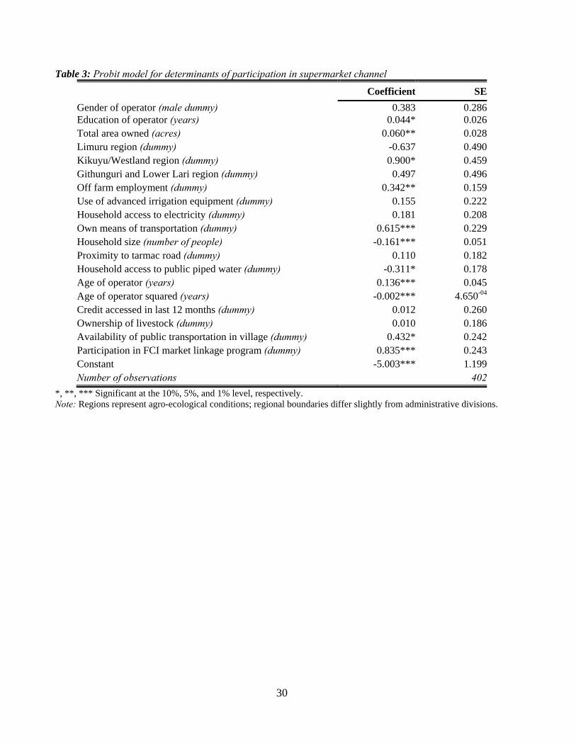
Results for determinants of participation in supermarket channels are presented in Table 3.

Alongside typical farm and household characteristics, we hypothesize that institutional support

through FCI enhances farmer access to supermarket channels. Therefore, we include

participation in the FCI market linkage program as an additional explanatory variable – defined

as a dummy. Yet, participation in that program might potentially be endogenous, which would

lead to a bias in the coefficient estimate. We test for endogeneity of the FCI dummy using a two-

18

step approach suggested by Rivers and Vuong (1988). Using membership in a farmer group,

which is correlated with FCI but not with supermarket channel participation, as an instrument,

we run a probit regression of FCI. Predicted residuals from this regression are then included as

additional explanatory variable in supermarket participation model and the null hypothesis to be

tested is that residuals are not significant – implying exogeneity of FCI variable. The test fails to

reject this null hypothesis (p = 0.664). So we proceed with the analysis assuming the FCI

variable to be exogenous. The probit model is estimated jointly with the income function using

endogenous switching model as illustrated under section 2.2.

Insert Table 3 here

The findings show that participation in supermarket channels depends on level of education and

age of the farmer. Better educated farmers are more likely to participate in supermarket channels.

Bette educated farmers tend to be more innovative and are therefore more likely to adopt modern

marketing channels. The relationship between age and participation in supermarket channels

assumes an inverted U-shape indicating that middle-aged farmers are more likely to participate

in supermarket channels.

Farmers who engage in off-farm employment are also more likely to participate in supermarkets.

This could be due to capital investment necessary for participation in supermarket channels

which is seemingly supported by income from off-farm activities. Ownership of land of land also

has a positive and significant influence on supermarket participation. This result should,

however, be interpreted with caution since as shown in the descriptive statistics, distribution of

land ownership does not vary much when we exclude the sample of farmers supported by FCI.

19

Access to public transport and ownership of means of transport also enhances farmers’ access to

supermarket channels. This result underscores the general importance of infrastructure in

meeting supermarket requirement for timely and regular delivery of vegetables.

Finally, institutional support by FCI has a positive and significant influence on supermarket

participation. FCI negotiates with supermarkets on behalf of farmers, facilitates collective

marketing approach by farmers and offers training to farmer groups on production technique and

supermarket requirements. This reduces transaction costs and makes smallholder farmers more

reliable trading partners for supermarkets. Equally important is the invoice discounting service

by FCI, which enables even relatively poor households with immediate cash needs to participate

in supermarket channels, despite the lagged payment schedule. These are important findings

from a policy perspective. Where no NGO like FCI is operating, public agencies might

potentially take on such roles of institutional support.

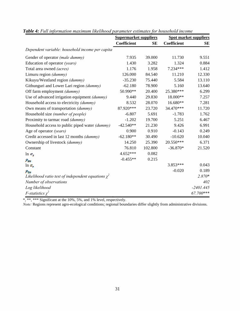
4.2 Income effect of participation in modern supply chains

While there could be limited access to supermarkets for disadvantaged farmers, those with access

could realize improvement in household income due to better price and steady flow of revenues.

Given possibility for systematic differences between farmers in the two channels, we expect

income responses to control variables to vary depending on market channels. Results for the

endogenous switching model are presented in Table 4. To identify the model, two variables in

the probit model – dummy for participation in FCI project and access to public transportation are

excluded from the income function.

Results indicate that suppliers to the two market channels indeed have incomes that differ

structurally from each other. For supermarket farmers, off-farm employment and ownership of

20

own means of transport have a positive and significant effect on household income per capita.

The significance of off-farm employment in both channel choice and income model for

supermarket suppliers is an indication of joint determination of income status and channel

choice. Off-farm employment also has a positive and significant impact on income per capita for

spot market suppliers but the effect is smaller.

Insert Table 4 here

Ownership of own means of transport is also significantly positive for both channels but the

effect is much higher for supermarket suppliers. This could be an indication of the activities that

the means of transport supports. For supermarket suppliers own cars are used for delivery of

vegetables to supermarkets which could be generating more returns than sport market suppliers’

activities supported by own cars.

Land ownership also influences income positively and significantly but only for spot market

suppliers. More land often implies more output and this can positively affect farm income

leading to higher household income. Farmers with more land can also lease out portions of their

land for income. Use of advanced irrigation technology also matters for income of spot market

suppliers. This could be an indication of self-selection into supermarket on the basis of use of

advanced irrigation technology. It is also an indication that spot market suppliers who use

irrigation have the chance to supply vegetable during off-season when prices are generally higher

and are thus able to generate more revenues than farmers without advanced irrigation

technology. Ownership of livestock also has a positive and significant effect on income for spot

market suppliers. In response to seasonal fluctuation in vegetable market especially in the

traditional channels, most farmers diversify into dairy activities where prices of milk remain

relatively stable. It is therefore likely that farmers facing uncertainty in vegetable markets will

21

diversify into dairy farming. Hence the relative importance of livestock keeping for spot market

suppliers.

The lower panel of Table 4 reports estimates for the covariance terms. The terms have similar

signs, which is an indication of “hierarchical sorting”. Supermarket suppliers therefore have

above average returns whether or not they participate in supermarket channels but are better off

in supermarket channels. The covariance estimate for spot market suppliers is, however,

insignificantly different from zero. Furthermore, since , we find evidence of self-

selection based on comparative advantage. Farmers with income above average per capita

income for supermarket suppliers therefore have higher than expected chances of participating in

supermarket channels. The model also fulfils the necessary condition for consistency

[ ]. Supermarket suppliers therefore earn higher income than they would earn if they

supplied traditional channels.

We also show the likelihood ratio test for joint independence of the three equations. The test

shows significant dependence between selection and income equations; thus indicating further

evidence of endogeneity. It is also important to note that in the absence of supermarket

participation, there would be no significant difference in average behavior of the two categories

of farmers caused by unobserved effects. This is evident from the insignificance of the

covariance estimate for spot market suppliers.

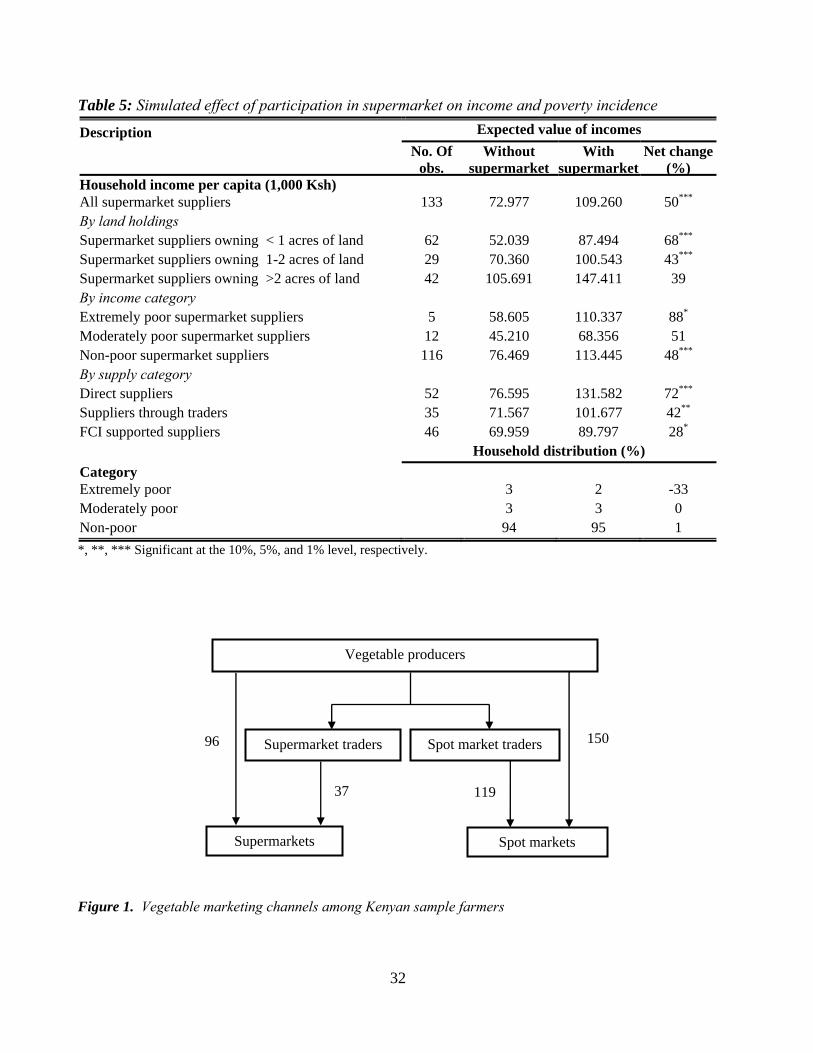
Finally we also estimate income effects as illustrated in equation (10). Results for estimation of

equation (11) are presented in Table 5, where effects are presented for different categories of

farmers. We also use the predicted household income to simulate poverty incidence. Poverty

incidence is estimated using predicted income with participation in supermarket channels. This is

22

then compared to potential poverty incidence that would be realized if supermarket suppliers

were supplying traditional channels. Results are shown in the lower panel of Table 5.

Insert Table 5 here

Results show significant gains in per capita income due to participation in supermarket channels.

This is true for the whole sample of supermarket suppliers and for different categories of

supermarket suppliers. For the whole sample of supermarket suppliers, participation in

supermarket channels yields a fifty-percentage increase in per capita income. However, smaller

farmers owning less than one acre of land and the extremely poor supermarket suppliers benefit

over-proportionally. Poorer farmers tend to engage largely in subsistence farming. Participation

in supermarket channels for such households thus provides an avenue for commercialization

farm activities leading to substantial gains in household income.

Farmers supplying directly to supermarkets also gain more from supermarket participation as

compared to their counterparts supplying through traders. In the absence of intermediaries, a

bigger share of price premium paid by high-value consumers accrues to producers leading to

significant gains for direct suppliers. The over-proportional gains in income for poor farmers

lead to larger significant reduction in poverty for the poorer category of supermarket suppliers.

These results should, however, be interpreted with caution since the proportion of poorer farmers

supplying supermarkets is quite small and may not reflect the general extent of benefit for the

wider poor households. The estimation also assumes constant characteristics of household in

alternative market channels. This is a strong assumption since we cannot guarantee that

supermarket farmers would exhibit similar characteristics if they were in spot market channels.

Nevertheless, the findings show that there is scope for improving household income via

23

participation in modern supply chains.

5. Conclusion

Increasing demand for high-value food commodities and resulting expansion of supermarkets in

developing countries is providing opportunities for farmers to participate in modern supply

chains. While stringent conditions by supermarkets may limit some farmers from accessing

supermarkets channels, participating farmers stand to gain substantially. Recent studies on high-

value chains in developing countries have looked into determinants of access and potential gains

from participation. However, these studies either adopt gross margin analyses which show no

causality or use treatment effect models that assume uniform effect across farmers in different

market channels.

Based on primary survey data of vegetable growers in Kenya, we find that better educated and

middle-aged farmers are more likely to participate in supermarket channels. Land and off-farm

employment which are indications of wealth status also increase the chances for participation in

supermarket channels by farmers. Supermarkets also favor farmers with better access to

infrastructure and those with own means of transport. More importantly, institutional support is

shown to enhance participation of farmers in supermarket channels.

Furthermore, we have also shown that participation in supermarket channels yields significant

income gains. Yet the two groups of farmers have different income structures. Since, our

analysis shows joint determination of income and supermarket channel choice, having accurate

information on income determinants is crucial in designing policies aimed at enhancing farmers’

access to high-value markets. Given the joint role of off-farm employment for instance, policies

supporting off-farm enterprises are likely to yield greater returns for spot market suppliers. Far

24

from directly improving household income, such policies would facilitate spot market suppliers’

access to high-value chains. This would lead to further improvements in household income –

producing a ripple effect of such income diversification programs. Consequently, there would be

significant reduction in poverty among farming households. These effects can particularly be

stronger given the overall importance of horticultural production in the Kenyan economy and the

likely spread of supermarkets to regional cities of the country.

More importantly we have shown that poorer farmers benefit over-proportionally from supplying

supermarkets. Yet it is this category of farmers who face the threat of exclusion from modern

supply chains. Interestingly, our analysis has also shown that institutional support enhances

farmer participation in supermarket channels. However, proper targeting of such institutional

support is necessary to ensure wider benefit by poorer households. This is particularly important

in light of the revealed self-selection of farmers into supermarket chains. Such targeted

intervention will become more crucial as supermarkets expand in the developing world and the

targeting can benefit from the accurate estimation undertaken here.

1. Recently, African indigenous vegetables have received renewed attention from upper and middle income consumers (Moore and Raymond, 2006; Ngugi et al., 2007).

2. Initially, supermarkets in Kenya purchased fresh vegetables in traditional wholesale markets, which can still be observed today. However, meanwhile supermarkets have diversified their procurement to include contracted farmers and traders, in order to ensure price stability and consistency in quality and supply.

25

References

Bolwig, S., Gibbon, P., and Jones, S. (2009). The economics of smallholder organic contract

farming in tropical Africa. World Development, 37(6), 1094-1104.

Dutoit, L. C., 2007. Heckman's Selection Model, Endogenous and Exogenous Switching Models,

A survey, Laure C Dutoit (bepress).

Fuglie, K. O., and Bosch, D. J. (1995). Economic and environmental implications of soil

nitrogen testing: A switching-regression analysis. American Journal of Agricultural

Economics, 891-900.

Greene, W. H. (2008). Econometric Analysis. Prentice Hall Upper Saddle River, NJ.

Hernandez, R., Reardon, T., and Berdegue, J. (2007). Supermarkets, Wholesalers, and Tomato

Growers in Guatemala. Agricultural Economics, Vol. 36(2007), 281-290.

International Bank for Reconstruction and Development. (2008). Global Purchasing Power

Parities and Real Expenditure: 2005 International Comparison Program. Washington,

D.C: The World Bank.

Lokshin, M., and Sajaia, Z. (2004). Maximum likelihood estimation of endogenous switching

regression models. Stata Journal, 4(282-289.

Maddala, G. S. (1983). Limited-dependent and qualitative variables in econometrics. Cambridge

Univ Pr.

26

Maddala, G. S. (1986). Disequilibrium, self-selection, and switching models. In Z. Griliches, and

D. Intriligator Michael, eds: Handbook of Econometrics Elsevier, NORTH-HOLLAND,

1633 - 1682.

Maertens, M., and Swinnen, J. F. M. (2009). Trade, Standards, and Poverty: Evidence from

Senegal. World Development, 37(1), 161.

Minten, B., Randrianarison, L., and Swinnen, J. F. M. (2009). Global Retail Chains and Poor

Farmers: Evidence from Madagascar. World Development, 37(11), 1728.

Miyata, S., Minot, N., and Hu, D. (2009). Impact of Contract Farming on Income: Linking Small

Farmers, Packers, and Supermarkets in China. World Development, 37(11), 1781-1790.

Moore, C., and Raymond, R. D. (2006). Back by popular demand: the benefits of traditional

vegetables: one community's story. Rome, Italy: IPGRI.

Moustier, P., Tam, P. T. G., Anh, D. T., Binh, V. T., and Loc, N. T. T. (2009). The role of farmer

organizations in supplying supermarkets with quality food in Vietnam. Food Policy, In

Press, Corrected Proof(

Ndeng'e, G., Opiyo, C., Mistiaen, J., and Kristjanson, P. (2003). Geographic dimension of well-

being in Kenya - Where are the poor? From district to locations. CBS, Ministry of

Planning and National Development, Kenya.

Neven, D., Odera, M. M., Reardon, T., and Wang, H. (2009). Kenyan Supermarkets, Emerging

Middle-Class Horticultural Farmers, and Employment Impacts on the Rural Poor. World

Development, 37(11), 1802-1811.

27

Neven, D., and Reardon, T. (2004). The Rise of Kenyan Supermarkets and the Evolution of their

Horticultural Product Procurement Systems. Development Policy Review, Vol. 22(6),

669-699.

Neven, D., Reardon, T., Chege, J., and Wang, H. (2006). Supermarkets and consumers in Africa:

the case of Nairobi, Kenya. Journal of International Food and Agribusiness Marketing,

18(1/2), 103-123.

Ngugi, I. K., Gitau, R., and Nyoro, J. K. (2007). Access to High-value Markets by Smallholder

Farmers of African Indigenous Vegetables in Kenya, Regoverning Markets Innovative

Practices Series. London: IIED.

Pingali, P., Khwaja, Y., and Meijer, M. (2007). The Role of Public and Private Sectors in

Commercializing Small Farms and Reducing Transactions Costs. In Johan F. M.

Swinnen, ed: Global Supply Chains, Standards and the Poor CAB International,

Cambridge, MA, 267-280.

Reardon, T., Barrett, C. B., Berdegue, J. A., and Swinnen, J. F. M. (2009). Agrifood Industry

Transformation and Small Farmers in Developing Countries. World Development,

37(11), 1717-1727.

Reardon, T., Timmer, C. P., Barrett, C. B., and Berdegue, J. (2003). The rise of supermarkets in

Africa, Asia, and Latin America. American Journal of Agricultural Economics, 1140-

1146.

Rivers, D., and Vuong, Q. H. (1988). Limited information estimators and exogeneity tests for

simultaneous probit models. Journal of Econometrics, 39(3), 347-366.

28

Trost, R. P. (1981). Interpretation of error covariances with nonrandom data: An empirical

illustration of returns to college education. Atlantic Economic Journal, 9(3), 85-90.

Warning, M., and Key, N. (2002). The Social Performance and Distrbutional Consequences of

Contract Farming: An Equilibrium Analysis of the Arachide de Bouche Program in

Senegal. World Development, Vol. 30(2), 255-263.

Willis, R. J., and Rosen, S. (1979). Education and self-selection. The Journal of Political

Economy, 7-36.

Wollni, M., and Zeller, M. (2007). Do farmers benefit from participating in specialty markets

and cooperatives? The case of coffee marketing in Costa Rica. Agricultural Economics,

37(2-3), 243-248.

29

Table 1: Differences between farmers supplying supermarket and spot markets

Variables Supermarket (133)

SD Spot market (269)

SD

Household and farm characteristics

Total area owned (acres) 2.692** 5.607 1.870 2.485Total vegetable area cultivated (acres) 1.168*** 1.457 0.697 0.992Share of vegetable area (%) 68.8* 31.9 62.8 32.5Use of advanced irrigation equipment (%) 87.9*** 32.7 71.4 45.3Age of operator (years) 47 12 49 15Educations (years of schooling) 10.3*** 3.14 8.72 4.05General farming experience (years) 16.16** 11.60 17.89 13.33Farmer participation in off-farm employment (%) 61*** 47 43 50Plot-level variables Fertilizer use (kg/acre) 362.56** 548.76 494.21 640.19Pesticide use (ml/acre) 2,251.22 4,083.44 2,745.51 4,382.22Purchased manure use (kg/acre) 15,926** 28,107 11,108 19,329Own manure use (kg/acre) 5,550 15,693 6,107 14,473Hired labor use (labor days/acre) 215.36** 296.29 164.28 276.98Family labor use (labor days/acre) 307*** 395 489 632Total labor use (labor days/acre) 522** 472 653 734

***,** and * Significantly different at 1% , 5% and 10% levels respectively a 1US dollar = 75 Ksh.

Table 2: Gross margin differences over market channels

Supermarket (n=133) Spot market (n=269)Mean SD Mean SD

Gross revenue (Ksh/acre) 116,636*** 129,370 73,179 60,136Seed cost (Ksh/acre) 2,175 5,428 1,660 3,021Hired labor cost (Ksh/acre) 6,330** 10,019 4,722 7,481Cost of other inputs Fertilizer (Ksh/acre) 4,846* 7,485 5,781 6,379 Purchased manure (Ksh/acre) 8,666*** 14,099 5,712 8,751 Pesticides (Ksh/acre) 1,104 1,922 1,179 1,835Other costs (Ksh/acre) 1,271** 4,723 623 2,167Net income (Ksh/acre) 92,244*** 114,202 53,502 54,677Family labor (Ksh/acre) 9,775** 21,297 13,951 16,570Own manure (Ksh/acre) 2,520 7,253 2,687 7,575Net income (Ksh/acre) 79,950*** 112,246 36,865 54,004

***,** and * Significantly different at 1% , 5% and 10% levels respectively a 1US dollar = 75 Ksh.

30

Table 3: Probit model for determinants of participation in supermarket channel

Coefficient SE

Gender of operator (male dummy) 0.383 0.286Education of operator (years) 0.044* 0.026Total area owned (acres) 0.060** 0.028Limuru region (dummy) -0.637 0.490Kikuyu/Westland region (dummy) 0.900* 0.459Githunguri and Lower Lari region (dummy) 0.497 0.496Off farm employment (dummy) 0.342** 0.159Use of advanced irrigation equipment (dummy) 0.155 0.222Household access to electricity (dummy) 0.181 0.208Own means of transportation (dummy) 0.615*** 0.229Household size (number of people) -0.161*** 0.051Proximity to tarmac road (dummy) 0.110 0.182Household access to public piped water (dummy) -0.311* 0.178Age of operator (years) 0.136*** 0.045Age of operator squared (years) -0.002*** 4.650-04

Credit accessed in last 12 months (dummy) 0.012 0.260Ownership of livestock (dummy) 0.010 0.186Availability of public transportation in village (dummy) 0.432* 0.242Participation in FCI market linkage program (dummy) 0.835*** 0.243Constant -5.003*** 1.199Number of observations 402

*, **, *** Significant at the 10%, 5%, and 1% level, respectively. Note: Regions represent agro-ecological conditions; regional boundaries differ slightly from administrative divisions.

31

Table 4: Full information maximum likelihood parameter estimates for household income Supermarket suppliers Spot market suppliers Coefficient SE Coefficient SE

Dependent variable: household income per capita

Gender of operator (male dummy) 7.935 39.000 11.730 9.551Education of operator (years) 1.430 3.282 1.324 0.884Total area owned (acres) 1.176 1.958 7.234*** 1.412Limuru region (dummy) 126.000 84.540 11.210 12.330Kikuyu/Westland region (dummy) -35.230 75.440 5.584 13.110Githunguri and Lower Lari region (dummy) -62.180 78.900 5.160 13.640Off farm employment (dummy) 50.990** 20.400 25.380*** 6.299Use of advanced irrigation equipment (dummy) 9.440 29.830 18.000** 7.257Household access to electricity (dummy) 8.532 28.070 16.680** 7.281Own means of transportation (dummy) 87.920*** 23.720 34.470*** 11.720Household size (number of people) -6.807 5.691 -1.783 1.762Proximity to tarmac road (dummy) -1.202 19.700 5.251 6.467Household access to public piped water (dummy) -42.540** 21.230 9.426 6.991Age of operator (years) 0.900 0.910 -0.143 0.249Credit accessed in last 12 months (dummy) -62.180** 30.490 -10.620 10.040Ownership of livestock (dummy) 14.250 25.390 20.550*** 6.371Constant 76.810 102.800 -36.870* 21.520

ln 4.652*** 0.082-0.455** 0.215

ln 3.853*** 0.043-0.020 0.189

Likelihood ratio test of independent equations χ2 2.870*Number of observations 402Log likelihood -2401.445F-statistics χ2 67.700***

*, **, *** Significant at the 10%, 5%, and 1% level, respectively. Note: Regions represent agro-ecological conditions; regional boundaries differ slightly from administrative divisions.

32

Table 5: Simulated effect of participation in supermarket on income and poverty incidence

Description Expected value of incomes

No. Of obs.

Without supermarket

With supermarket

Net change (%)

Household income per capita (1,000 Ksh) All supermarket suppliers 133 72.977 109.260 50***

By land holdings Supermarket suppliers owning < 1 acres of land 62 52.039 87.494 68***

Supermarket suppliers owning 1-2 acres of land 29 70.360 100.543 43***

Supermarket suppliers owning >2 acres of land 42 105.691 147.411 39 By income category Extremely poor supermarket suppliers 5 58.605 110.337 88*

Moderately poor supermarket suppliers 12 45.210 68.356 51 Non-poor supermarket suppliers 116 76.469 113.445 48***

By supply category Direct suppliers 52 76.595 131.582 72***

Suppliers through traders 35 71.567 101.677 42**

FCI supported suppliers 46 69.959 89.797 28*

Household distribution (%)

Category Extremely poor 3 2 -33 Moderately poor 3 3 0 Non-poor 94 95 1

*, **, *** Significant at the 10%, 5%, and 1% level, respectively.

Figure 1. Vegetable marketing channels among Kenyan sample farmers

Vegetable producers

150 96 Spot market traders Supermarket traders

37 119

Spot markets Supermarkets

33

0.2

.4.6

.81

Cum

mul

ativ

e fr

actio

n of

hou

seho

lds

0 100 200 300 400 500Gross margin per acre (1000 Ksh)

Supermarket suppliers Spot market suppliers

Figure 2: Cumulative distribution of gross margin by market channel (K-S D-statistics =0.170 (p=0.009))

Figure 3: Average per capita income by market participation

34

0.2

.4.6

.81

Cum

mul

ativ

e fr

actio

n of

hou

seho

lds

0 100 200 300 400 500Per capita household income (1000 Ksh)

Supermarket suppliers Spot market suppliers

Figure 4: Cumulative distribution of per capita household income by market channel (K-S D-statistics =0.361 (p=0.000))

Figure 5: Incidence of poverty by market participation

35

Figure 6: Distribution of land ownership by market participation