Theor. Comput. Fluid Dyn. (2018) 32:689–711https://doi.org/10.1007/s00162-018-0473-1

ORIGINAL ARTICLE

M. Staszak

Superficial transportation model using finite volume method

Received: 19 December 2016 / Accepted: 20 July 2018 / Published online: 28 July 2018© The Author(s) 2018

Abstract The work presents a new modeling technique designed for transporting selected property whilesimultaneously tracking particular value of certain field variable. The model addresses the problem of trans-portation of superficial properties according to fluid/fluid interface evolution. Such problem arises when somesuperficial variable needs to be attached to the evolving interface or front defined. Several multiphase modelsin CFD technique lack such ability. The model proposed is illustrated by the experimental two phase systemof toluene/water with surfactant specie (sodium dodecylsulfate SDS). The selected superficial property thatis important to be tracked according to interface evolution is Gibbs surface excess. The computation wasperformed using Ansys/Fluent software with proposed models created and attached using C programminglanguage.

Keywords Interface mass transfer · Adsorption · Liquid–liquid interfaces · Fluid dynamics

List of symbols

A Area (m2)Asz Szyszkowski isotherm coefficient (mol/m3)Bsz Szyszkowski isotherm coefficient (–)c Concentration (mol/m3)D Diffusion coefficient (m2/s)F Force (N)g Acceleration due to gravity (m/s2)G Gibbs free energy (J)J Mass flux (mol/m2s)k Coefficient for modified Weibull function (1/s)m Mass (kg)n Unit normal vectorNf Number of cell facesP Pressure (Pa)R Curvature radius (m)S General volumetric source term [mol (units of ø)/(m3 s)]t Time (s)

Communicated by Tim Phillips.

M. Staszak (B)Institute of Chemical Technology and Engineering, Poznan University of Technology, Pl. Skłodowskiej-Curie 2,60-965 Poznan, PolandE-mail: maciej.staszak@put.poznan.pl

690 M. Staszak

u, w, v Velocity components of its magnitude (m/s)u Coefficient for modified Weibull function (mol/m2s)v Coefficient for modified Weibull function (mol/m3)V Volume (m3)We Weber number

Greek letters

ø General scalar quantityα Phase volume fractionη Viscosity (Pa s)Γ Gibbs surface excess (mol/m2)γ Interfacial tension (N/m)κ Local interface curvature (1/m)λ Coefficient for modified Weibull function (mol/m3)ρ Phase density (kg/m3)τ Viscous stress tensor (Pa)υ Velocity (vector) (m/s)Θ Contact angle (◦)ω Angular velocity component (1/rad)

Subscripts

ads Refers to adsorptivecell Refers to single cellf Refers to face centered valueø Refers to general scalar quantityp Refers to pth phaseq Refers to qth phases Refers to surface valuex, y, z Cartesian coordinates

1 Introduction

Interfacial phenomena are the subject of investigation in many branches of the industry. The phenomenaoccurring on the interface are analyzed in this work by the model proposed using experimental conditionswhich are good test for proposed modeling method. The evolving and aging interface during the process ofdrop formation is connected with the effects of changing interface curvature along with its physical propertiesfrom which the most important are surface excess and interfacial tension. In addition, the process of dropformation which is analyzed in this work has a great significance in several fields. The typical areas are thepurification extraction processes [1–3], metallurgic processes of gas metal arc welding [4], emulsificationprocesses [5–7], jet print processes [8–10], the oxygenation of blood equipment design [11,12] or pool boilingbubbles spreading [13] and manufacturing liquid microcapsules by centrifugal extrusion or spray drying [14].Besides the pendant drop, the CFD simulation of liquid drops in different conditions is treated in literature,e.g., drop flow, impact, spreading, sliding, solidification on solid surfaces [15–21], the process of a liquid dropformation in the coaxial capillars [22], the effects of local interfacial nonhomogeneity due to local surfaceactive specie concentration differences [23]. The problems of liquid drop oscillations is analyzed in other worksof the authors [24,25]. The analysis of water–octane system [26] using commercial software FLUENT in 3Ddomain showed the model deviation is below 5% of relative error in a drop life time and its volume. Becausethe problem of multiphase flows and accompanying superficial effect are still being investigated, expandingthe modeling capabilities of existing models of fluid/fluid interface has not only scientific and explorativesignificance but also may extend the capabilities of a designer’s tools.

An appropriate description of the surface processes allows to achieve more accurate predictions and conse-quently leads to a better understanding and utilization of the surface phenomena. The drop shape measurementis a good test for interface models because any model discrepancy can easily be detected in the condition of

Superficial transportation model using finite volume method 691

growing and aging a pendant drop. Moreover, it provides the opportunity to capture interface phenomena withhigh accuracy. Several techniques in laboratory practice, e.g., the capillary rise, Wilhelmy plate method, DuNoüy ring method, drop weight method, pendant/sessile drop and bubble methods, spinning drop method, orthe maximum bubble pressure method are all derived for interface examination and research.

This work presents the extension to computational fluid dynamics volume of fluid model which allowtaking into account the surface phenomena on the fluid/fluid interface. The key innovation proposed is thealgorithm of superficial property transport along with the interface dynamic evolution. The original, typicalmultiphase VOF transient model allows only to describe interface only at current time step by its primaryproperty—surface tension. It is not possible to use the typical VOF approach when calculation of dynamicevolution of interface requires that previous time step and previous interface location to be known for givenproperty calculation. In other words, it is not possible to attach any field variable to specified interface locationlocally and translocate it together with its movement. At given time step, the VOF model is not able to locateprevious time step locations, and previous time step values of any interface variable. The previous time stepinterface position in space and coupled with this location superficial variable must be known to describe someprocesses properly, for example in the case of interfacial adsorption of surfactants. One of the fundamentalthermodynamic variables for the cases when surfactants are involved, is the Gibbs surface excess Γ , a quantitydescribing superficial concentration of adsorbed, surface active specie [27]. The dynamic simulations in theCFD technique are based on the time stepping algorithms which are applied by various numerical schemes.The calculation of surface excess Γ for current location on the liquid interface and for current time step canonly be done referring to previous time step and previous location values. Due to this requirement and takinginto account that well-known VOF algorithm contains no methods nor techniques for attaching any physicalproperty to the interface, the proposed model is a useful extension allowing to simulate the surface excessdynamic advancement.

The Eulerian frame of reference of the VOFmodel reasons the need of interface reconstruction on the basisof specific color function. A locally defined surface tension, Gibbs surface excess and interfacemass flux vectorneed to evolve according to the interface evolution. Proposed approach introduces lagrangian reference frameto the description of the interface by the use of markers indicating the surface position and time evolution.The set of markers is then translated according to the velocity field and phases volume fractions field. Themarkers might be thought of as a lagrangian virtual particles that translocate with the fluid elements. In thepresent work, they are independent from the underlying grid and are used to carry local information aboutthe interface. The marker and cell (MAC) method is known in literature and was investigated to keep trackof the front shock waves (shock-capturing methods) or interfaces between fluid phases. There are algorithmswhich rely on the use of particles to track desired variable or flow property. Some of the examples are theMACmethod [28] and its several variants: SMAC [29] (simplified marker and cell), GENSMAC [30] (generaldomains simplified marker and cell), GSMAC [31] (generalized simplified marker and cell).

Similar to the presented works above, there are hybrid methods that combine the VOF andMAC techniquesto achieve specific aims. Aulisa [32] utilizes concept of conservation markers to construct the interface. Thealgorithm is focused on correcting the interface calculated by standard VOF method to preserve its area. Theirother works [33,34] focus on algorithm for the reconstruction and advection of interfaces using marker andcell grid but limited to the two-dimensional space. Enright [35] puts two sets of markers called “positive” and“negative” at either side of the interface to rebuild the region for specific cases that otherwise stay underresolvedgiving unrealistic geometric interface topologies. Durikovic [36] presents technique of multifluid (more thantwo phases) VOF simulation discretized on MAC grid. The technique is used mainly for visualization andanimation purposes. The most similar to presented work use of markers with VOF model is the correctivealgorithm proposed by Lopez [37]. The markers are placed at the midpoints of the reconstructed cell interfacesegments and are used to resolve the flow characteristic smaller than grid size. Typical usage of this approachis to account for the small fluid filaments creation phenomena.

The model proposed makes use of the Lagrangian method of fluid dynamics [38]. This technique utilizesan collection of virtual Lagrangian particles of zero spatial size whose paths in space are governed by thevelocity field. The velocity field which are utilized to move the particles originates from CFD core algorithmimplemented in Ansys/Fluent. The tracks of virtual particles map the streamlines of the velocity field, correctedat every numerical time step by the location of selected isovalue of volume fraction. By following the flow ofvirtual particles, and assigning a specified superficial variable (and possibly other properties) to them duringcalculations, the problemof interfacial properties translocation and their time evolution is addressed and solved.

Lagrangian approaches are extensively utilized in engineering, including discrete element methods [39]and smoothed particle hydrodynamics [40]. The Lagrangian structure for studying pathways corresponds to

692 M. Staszak

the analysis of tracers. One of the significant dissimilarities is the computational cost. For each time step,translocation of a Lagrangian particle takes only one calculation route of relatively simple computations.On the other hand, considering the advection–diffusion of a selected tracer variable, it takes several steps ofcomputation to estimate its trajectory.

2 Modeling the interface

The concept of Gibbs dividing plane [41] is essential when defining the surface excess Γ of surfactant. Theimportance of the shape of the interface was realized and analyzed by Gibbs [42], Guggenheim [43], Gurtin[44], Oversteegen [45] and others. The position of dividing plane impacts the perceived surface excess value,and its location is chosen to conform with its zero value for clean solvents [46]. Most of computationalfluid dynamics multiphase models present the interface as a surface geometrical manifold of an infinitesimalthickness which is located in the area of sudden change of physical and chemical parameters. Presence of suchinterface in the simulated case is a good testing environment for the algorithm for superficial property timeevolution.

The formulation of theCFD technique involves the classicalNavier–Stokes set of equations,which originatefrom Newton’s Law of Motion:

∂ (ρ �υ)

∂t+ ∇ · (ρ �υ �υ) = −∇ p + ∇ · (τ ) + ρg + �F (1)

The mass conservation (or continuity equation) is used for total mass balance:

∂ρ

∂t+ ∇ · (ρ �υ) = �m (2)

The dynamic evolution of the interface as a result of the force and, consequently, the velocity field influencecan be simulated using several approaches in CFD. The front tracking methods [47], level set methods [48]and volume of fluid methods [49] are the most commonly used ones for interface modeling. For the purposeof interface capturing Eq. (3), which specifies the evolution of the volumetric amount of the phase containedby the cell, is introduced in addition to the above. This quantity is the volume fraction α of a given phase, andthe sum of all phase volume fractions in a given volume must equal one.

∂αqρq

∂t+ ∇ · (

αqρq �υq) = Sαq +

n∑

p=1

(m pq − mqp

)(3)

The explicit spatial discretization of geometric reconstruction was applied to the equation (so called Geo-Reconstruct). It is the most accurate and precise scheme available in Fluent, which unfortunately is morecomputationally demanding than the other schemes. Geo-Reconstruct is the best scheme when using low-quality meshes. The time advancement scheme chosen for this work is an explicit formulation. It is noniterativefor given time step and is time-dependent scheme. It reveals better numerical accuracy compared to the implicitformulation, which is burdened with negative numerical diffusion phenomena. Though the time step sizemight be severely limited by a Courant number, typical stability criterion used in VOF modeling. Solution toEq. (3) contains a discontinuity which is expressed as sudden jump of computed quantity α in the locationof the interface. Such nondiffusive multiphase continuum as a limiting case of differential diffusion transportequation is studied by Mellado et al. [50]. Several algorithms are utilized to reconstruct the interface, havingsolved the distribution of α in the space [51–56].

The force source �F generated by the interfacial tension at the interface is important quantity during interfacereconstruction. Brackbill et al. [57] proposed the continuum surface force method which is based on the theorythat the pressure jump across the interface is proportional to the curvature of the interface κ and the interfacialtension, according to the Young–Laplace equation:

p2 − p1 = γ κ (4)

Thewall adhesion and, consequently, contact angle θ play also significant role in determining the fluid behaviorin the location of the fluid–fluid–wall contact line. The contact angle is accounted for by the use of formula(5) for unit vector n normal to the interface at the wall contact point.

n = nw cos θw + nt sin θw (5)

Superficial transportation model using finite volume method 693

nt is a normal vector to the contact line between the interface and the wall at the contact point and nw is theunit wall normal directed to the wall. Implementation of the contact angle into fluid dynamics simulations maypose some serious difficulties as presented by Linder et al. [58].

In this work, the two immiscible liquids system is experimentally analyzed and used to make verification ofthe model proposed. In the system examined, the liquid droplet of heavy phase is formed into the lighter liquidphase. Several studies are devoted to simulation of droplet formation and its behavior [59–61]. In this work, theexperimentally examined toluene–water system with sodium dodecyl sulfate (SDS) as a surface active speciewas a base to validate the superficial transportation model proposed. The fundamental motivation for studyinginterface surfactants activity at liquid–liquid interface is to describe the process of liquid–liquid phase transfercatalysis by means of CFD. This process is a key element in interface chemical reactions in many industrialprocesses that involve green methodology [62,63].

3 Bulk phase mass transfer

The description of component mass transfer in model proposed is divided into two different mechanisms andconsequently two distinct calculation approaches. The bulk phase and near-interface mass transfer differ dueto different nature of driving forces. The calculations performed in this work utilize the Fickian approach forbulk diffusion [64–66]. The bulk phase binary diffusion coefficient of sodium dodecyl sulfate through waterwas calculated using Siddiqi–Lucas correlation which was derived based on over 600 different water solutions[67]:

Di,w = 2.98 × 10−7V −0.5473i η−1.026

w T (6)

The above correlation is based on metric units and expresses diffusion coefficient in cm2/s. The value of SDSmolecular volume Vi was taken from literature [68]. The component flux is then calculated using Fickianapproach:

�Jbulki = −ρDi,w∇xi (7)

In the case of multiphase flow, the equation of fluid motion (1) and continuity (2) are additionally accompaniedby the species mass balance equation for component i and given phase j :

∂(α jρ j xi

)

∂t+ ∇ · (

α jρ �υxi) = ∇ ·

(α j �Jbulki

)+ �mi (8)

The equation above is solved for spatial locations where the j th phase exists. In location of interface, the weightof the transport is minimized by the value of volume fractions α j . In that case, near the interface, adsorptivemass transfer is main transportation mechanism.

4 The near-interface adsorptive flux computation

The key part of model proposed, where the markers introduced are involved, is the way the mass flux due toadsorption is calculated. The near-interface location is understood inmodel proposed as a set of cells containingthe calculated, reconstructed interface. Unlike the bulkmass transfer, themass flux near the interface is inducedmainly by adsorption of surface active component. Applying appropriate mass transfer approach, expressedin modification either in diffusion coefficients or model equations themselves, is typical to describe the masstransfer in any media, where concentration gradients do not generate dominant driving force (e.g., ions flux inpresence of electric field) or in caseswheremolecular diffusion coefficients are not known and are substituted byeffective diffusivities [69–71]. Calculating adsorptive near-interfacemass transfer creates the need for effectivediffusion coefficient estimation. First approach to dynamics of the interface adsorption was presented byWardand Tordai [72] who formulated first quantitative model of diffusion controlled adsorption, then the mixedadsorption kinetic model proposed by Baret [73] and, further, short and long time approximations proposedby Feinermann [74]. The thermodynamic description of system containing interface in the form of free energyfunctional is widely discussed [75–79] and also the detailed presentation of the models used to describe theadsorption processes at the liquid–liquid interfaces can be found in literature [80]. Such formulations give theadsorption dynamics description in a form similar to originalWard and Tordai equation but without assumptionthat initial surface excess is equal zero [81].

694 M. Staszak

Fig. 1 Szyszkowski isotherm of SDS equilibrium data

The significant part of the model proposed in this work is the ability of computation surface active com-ponents interface mass flux without the use of diffusion coefficients. In order to compute the interfacial massflux generated by adsorption forces, it is formulated according to specific interface description. Previouslymentioned Fickian relationship for bulk phase relates diffusion coefficient with concentration gradient. In thevicinity of the interface, the adsorptive diffusion flux is given by:

Jads = −Dadsdc

dx(9)

Which is then modified by applying Gibbs surface excess to give known relationship:

Jads = dΓ (t)

dt(10)

The above formulation introduces the surface excess as a time-dependent function Γ (t). The mass flux thatdirects into the interface is given by the change of surface excess in corresponding time period so to be mostaccurate a proper definition of such a function is later in the text proposed. The values ofΓ (t) at consecutive timesteps must be determined in order to estimate the derivative dΓ (t)/dt . Such function can easily be estimatedwith the use of Szyszkowski [82] isotherm coefficients although other similar isotherms (like Frumkin) couldalso be applied. To make distinction between functional forms and experimental data of the same quantities inthe text, the subscript exp is added wherever experimental ones are used. The experimental values of interfacialtension γ exp are related with corresponding bulk concentrations cexp by Szyszkowski isotherm:

γ Szexp = γ0

(1 − Bsz ln

(cexpAsz

+ 1

))(11)

Based on the experimental measurements of the interfacial tension γ Szexp for different bulk concentrations

cexp, the values of Asz and Bsz coefficients are determined. This is done using least-squares method so theSzyszkowski curve fits the experimental data [83]. Figure 1 presents typical data acquired for SDS and cor-responding, fitted using Szyszkowski isotherm. The experimental points are obtained on the basis of 600continuous measurements, and corresponding statistical error is so small (between 10−4 and 10 −5 N/m) thatit is not presented on the graph.

The experimental values of a surface excess are estimated from the equation:

Γexp = Bszγ0c

RT (c + Asz)(12)

The bulk concentrations are calculated by the rearrangement of Szyszkowski equation:

c = exp

(γ Szexp − γ0

γ0Bsz

)

Asz − Asz (13)

Superficial transportation model using finite volume method 695

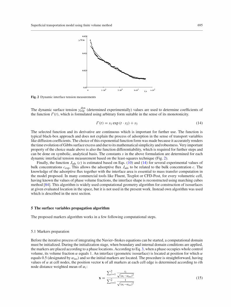
Fig. 2 Dynamic interface tension measurements

The dynamic surface tension γdynexp (determined experimentally) values are used to determine coefficients of

the function Γ (t), which is formulated using arbitrary form suitable in the sense of its monotonicity.

Γ (t) = s1 exp (t · s2) + s3 (14)

The selected function and its derivative are continuous which is important for further use. The function istypical black-box approach and does not explain the process of adsorption in the sense of transport variableslike diffusion coefficients. The choice of this exponential function formwasmade because it accurately rendersthe time evolution ofGibbs surface excess and due to itsmathematical simplicity and robustness.Very importantproperty of the choice made above is also the function differentiability, which is required for further steps andcan be done on symbolic, analytical basis. The constants s in the above formulation are determined for eachdynamic interfacial tension measurement based on the least-squares technique (Fig. 2).

Finally, the function Jads (c) is estimated based on Eqs. (10) and (14) for several experimental values ofbulk concentrations cexp. This allows the adsorptive flux Jads to be related to the bulk concentration c. Theknowledge of the adsorptive flux together with the interface area is essential to mass transfer computation inthe model proposed. In many commercial tools like Fluent, Tecplot or CFD-Post, for every volumetric cell,having known the values of phase volume fractions, the interface shape is reconstructed using marching cubesmethod [84]. This algorithm is widely used computational geometry algorithm for construction of isosurfacesat given evaluated location in the space, but it is not used in the present work. Instead own algorithm was usedwhich is described in the next section.

5 The surface variables propagation algorithm

The proposed markers algorithm works in a few following computational steps.

5.1 Markers preparation

Before the iterative process of integrating the Navier–Stokes equations can be started, a computational domainmust be initialized. During the initialization stage, when boundary and internal domain conditions are applied,themarkers are placed according to a phase locations. According to Eq. 3, when a phase occupies whole controlvolume, its volume fraction α equals 1. An interface (geometric isosurface) is located at position for which αequals 0.5 (designated by αiso) and so the initial markers are located. The procedure is straightforward, havingvalues of α at cell nodes, the position vector x of all markers at each cell edge is determined according to i thnode distance weighted mean of αi :

x =∑2

i=1xi√

(αi −αiso)2

∑2i=1

1√(αi −αiso)

2

(15)

696 M. Staszak

Fig. 3 Construction of initial markers

The locations x of edge markers located at αiso are then averaged to give initial markers locations in the cellinterior. The situation when αiso equals αi means that the interface is located exactly at specified node of thecell. This condition, if happens, is handled by the code by if-then clause. Figure 3 presents the edge markers� created using Eq. (15) and initial markers • used for further computations. The edge markers are discardedafter initial ones are created. Such preparation technique ensures that the initial markers are located at a cellinterface superficial elements centroids. This does not prevent them from clustering in the case when interfaceis located near one of the cell edges. This algorithm does not address such behavior as it has no impact onsurface variables propagation and most important, it ensures that every cell in which interface is located has itsown marker. At the final stage, for every cell containing the marker, the adsorption model, presented before,is computed to give superficial values of component surface excess. This value is stored at marker for furtherprocessing.

5.2 Markers projection

The algorithmofmarkers relocation is designed to follow the stepwise approach of interface transient evolution.Based on the original/initial locations of markers evaluated at previous time step and current time step interfacelocation, the advancement procedure is performed. The superficial variable specified for previous time stepand recorded at each marker has to be moved to new location of the interface. For this reason, a new spatialcoordinates of the markers are calculated to locate actual, new position of interface. Each marker has itscorresponding, individual velocity vector specified, and such a vector indicates the direction of advancementand relates previous to actual superficial variable position. However, the momentum equation is most oftensolved using different scheme of discretization when compared to the discretization of mass balance for givenphase. For this reason, the new coordinates found by velocity vector might not exactly be the same as the newposition of the interface. On the range of one time step, this discrepancy is very small but may increase duringsuccessive and repeated time steps. At this stage, the new set of markers (second, auxiliary set) is created at theexact location of the interface using the same method as described in the previous section. The two markerssets are kept in memory in order to copy the values of superficial variable from first markers relocated on thebasis of velocity vectors to the new markers created on the actual interface. At this moment, it is important toassociate markers from the first set with the appropriate new markers created. Such logic link between eachmarker from first set and each actual interfacial marker is required to perform the advancement of superficialvariable in correct and appropriate direction. The link between the initial marker and actual marker is createdon the basis of distance matrix using nearest neighbor algorithm. The two sets of markers are in close vicinity,typically in the distance much smaller than size of a single cell, but this is not a requirement because markersare not connected to mesh in any way. After the values of superficial variable are copied to the second markers,the first markers are discarded, the memory is freed, and the second set becomes actual set of markers, locatedat new interface position, containing the translocated value.

Superficial transportation model using finite volume method 697

5.3 Transported quantity

This is important to note that the algorithm presented is suitable only to transport an intensive quantity due tobalance considerations for computational mesh cells which have different volumes. The component surfaceexcess is intensive quantity which is updated at every time step by the adsorption model described earlier inthe text. Having computed the flux Jads of surface active specie into the interface, the value of surface excessis updated accordingly by the time advancement formula:

Γt+�t = Γt + Jads�t (16)

In the case when the interfacial mass transfer is involved, the corresponding number of component moles areremoved from the local cell containing the interface. The i th specie mass source (sink) is defined:

�mi = −Jads · SintVcell

(17)

and expresses the mass that is transported to the interface area Sint due to adsorptive flux in the cell volumeVcell. The �mi is the source term included into the species mass balance equation Eq. (8).

The Ansys/FLUENT software allows to link own model, being an extension to existing CFD code, atdifferent stages of a solution process. The attachment of the model procedures is allowed in a variety ofcomputational states, for example for already available phenomena models, numerical states or geometriclocations and in many other situations. The code that is written in C programming language is compiled inAnsys environment and then attached to the CFD computational core, for example at geometric boundaries asboundary conditions, in fluid volume as source terms, or in some specific point of computation like at the endof a numerical iteration. Such user-defined functions (UDF) were used in this work to formulate the describedmodel and is attached to execute at the end of every numerical iteration (execute_at_end UDF function). Theprocedure loops over every mesh cell in a calculation domain and locates the cells containing the interface.For those cells, the calculations of the algorithm of the adsorptive mass transfer model are performed. Theschematics of the procedure proposed are presented in Fig. 4.

Themarkers are programming objects defined as structured type that aggregates a fixed set of different typesobjects into one single object. The marker object structure contains: its location defined as three-dimensional

Fig. 4 Calculation scheme for proposed model of adsorptive mass flux and interface variables propagation

698 M. Staszak

Fig. 5 The volume used in the artificial surface diffusion test

vector of real values, surface Gibbs excess and unique volume cell index identifying computational cellcontaining interface.

6 Superficial mass balance and numerical diffusion

A test simulation to perform a verification of the superficial mass conservation and numerical diffusion wasprepared. In a cuboid domain (0.1× 0.1× 0.1m), a two phase air–water system was defined and slow upwardmotion was applied by the inlet boundary located at the bottom. The vertical fluid movement was introducedto exert a momentum forces on the surface and to observe the superficial variables evolution under dynamicconditions. Actually, the surface excess Γ is the superficial, transported variable in the model proposed butfor the test a unity value (g = 1) was applied instead. The test values g = 1 were distributed onto half of theinterface S1 (see Fig. 5) while setting the rest of the space with zero value (g = 0). A fluid velocity 0.001m/sand 10s of simulation time moved the surface upward enough to allow observation of superficial distributionof values applied initially. The algorithm proposed is not supposed to apply any surface diffusion component,but artificial diffusional effect is possible. To estimate the quantitative numerical effect of artificial diffusioncomponent, the surface integral mean over the interface of transported testing values was calculated at everytime iteration:

Gi =∫

Si

g

SidSi (18)

The integral (18) defines total value of g over the surface part Si located in given part of the volume (Fig. 5).Any change of the averaged integral value Gi indicates artificial diffusion effect between the volumes. Thetotal sum of Gi for both parts of the interface should result a unity value; any deviation from this value willindicate mass imbalance.

Actual results for the test performed are presented on graph in Fig. 6 showing surface average integralsof test value gi . The curves represent the actual, recalculated for percentage scale, surface average of valueGi . The ideal and expected values (for the case of no artificial diffusion) should obtain 100% for S1 (absolutevalue of G1 = 0.005m−2 due to the size of the domain) and 0% for S2 (absolute value of G2 = 0.0m−2).Any deviation from those two values shows the numerical imbalance which is caused by artificial diffusion.

Figure 6 shows typical character of any finite element method applied to given problem. The higher isthe number of finite elements, which in the case of the CFD technique are finite volumes, the higher is theaccuracy of results obtained. The results of the test performed (Fig. 6) show that the numerical imbalance andartificial diffusion, which is measured as deviation from value of 100% for S1 and 0% for S2, is smaller forhigher number of markers. Higher loss of mass is observed for number less than 4000 markers. The artificial

Superficial transportation model using finite volume method 699

Fig. 6 The surface average integral of test value g for both part of the surface analyzed: S1 and S2, used in the artificial surfacediffusion test

diffusion is visible for the parts where S1 curve minimizes with corresponding S2 curve increase (from 2000to 4000 of markers). This indicates mass being transported unintentionally from the S1 to the S2 area. The testillustrates that such negative numerical effects of the algorithm proposed can be minimized by using highernumber of finite elements during the calculation.

The visible error of the balance is mainly related to the VOF model used in this work. The markers followthe interface in accurate and exact way, tracking its position in every time step. Thus, the main source of theimbalance lays in the VOF numerical instability, namely spurious currents which affects the interface stability.This negative effect is caused by the VOF model assumption to use single, common velocity field approach.This phenomena is known as disadvantage of VOF method which becomes more visible for low velocities.In the example presented, it is deliberate to render the situation which is difficult from the modeling pointof view. The low velocity of the interface transition which was applied in the case presented is typical setupfor which such a model can be tested by drop volume method. There is possibility to make a choice of anyother multiphase approach, where the limitation of common velocity field is not imposed. But because of thepopularity of VOF model, this work is focused on the possibility to extend this approach with all its benefitsand disadvantages.

7 Experimental part

A system of two immiscible liquids (toluene and water+SDS) was chosen for the verification of the CFDsimulation. The Tracker tensiometer was used to perform the drop shape experiments. Seven samples atdifferent SDS concentrations were submitted into the tests to build Szyszkowski isotherm. The twice distilledwater was used as the aqueous and twice distilled toluene as organic phase. Samples were shaken for 4hto assure equilibrium state at the interface. The measurements were carried out at 25 ◦C. Measurements arein general accordance to other works [85,86]. The fit goodness, measured as a square error, for the isothermequals 4.367×10−6 which gives about 2mN/m isothermmean deviation from the experimental values. Takinginto account that determination coefficient for that isotherm is at value 0.963 which means that the isothermexplains 96.3% of all measured data, such accuracy assures that the Szyszkowski isotherm is a good descriptionof the system.

The A and B coefficients of Szyszkowski isotherm were found to be 7.736× 10−4 and 0.069 accordingly.Following previously described procedure theSDSmassfluxeswere computed for different bulk concentrations(Table 1).

The values of flux were then related to bulk concentrations by the use of modified Weibull [87] function(19) by means of least-squares approximation.

J (c) =(

k · (c − v) · exp(

v − c

λ

)+ u

)× 10−12 (19)

700 M. Staszak

Table 1 Computed SDS mass stream fluxes for different bulk concentrations

c (mol/m3) J (mol/m2s)

0.035 1.043 × 10−11

0.052 6.366 × 10−12

0.347 2.759 × 10−12

0.520 2.962 × 10−12

5.201 8.142 × 10−12

Table 2 Calculated coefficients values for Eq. (19)

k (1/s) v (mol/m3) λ (mol/m3) u (mol/m2s)

−80.99 0.216 0.049 7.998

Fig. 7 Contact angle versus surface tension for toluene–water–metal capillary contact point

Table 3 Calculated coefficients values for Eq. (20)

u1 (◦) u2 (m/N) u3 (◦)

−62.203 −82.958 151.32

The values of adjusted coefficient used in flux J calculation are given Table 2.It was mentioned earlier that adhesion forces at the domain boundaries have major impact on the interface

formation process. Incorporating the contact angle between the fluids and a solid wall was done by definingthe contact angle θ at the wall by formula (5). Experimental data shows tendency of exponential growth ofcontact angle by increasing surface tension (Fig. 7).

The contact angle was related with surface tension by exponential function fitted to the obtained experi-mental values:

θ(γ ) = u1 exp (γ · u2) + u3 (20)

The calculated by the least-squares method values for the equation according to experimental data presentedin Fig. 5 are given in Table 3.

8 Modeling details

A finite elements domain rendering the capillary and surrounding volume was created using tetrahedral ele-ments in three-dimensional space. The mesh element size must be chosen in such a way to be able to reproducethe specifics of the flow; here, the drop shape and consequently surface adsorption process itself. To renderthe specifics of the experimental cuvette setup the cubic shape space was created. The dimensions of the cubewere chosen such to be able to receive and hold an investigated drop geometry. The cross section of the volumeis presented at Fig. 8, the detailed view presents the capillary tip geometry. It is visible that the circular shape

Superficial transportation model using finite volume method 701

Fig. 8 Cross section of the finite element model; detailed view A shows capillary tip (∅1.3mm) rendered by tetrahedrons. Thewhite, checkered lines indicate the position of boundaries applied to the model

is well reproduced by the triangles on upper face and tetrahedrons in the interior. The base size of an elementwas set to 0.00005m; which gives about 400.000 elements in the cubic volume of size 8×8×8mm. To reduceamount of computing work required to solve the field variables, more elements of smaller size are located nearthe capillary tip by applying a sizing function. More coarse mesh located in the remaining region is satisfactoryto render the specifics of the surrounding flow.

Appropriate boundary conditions were applied to the volume bounding faces. Typical wall boundarycondition with no slip hydrodynamic condition was applied to the side and bottom faces. Top face was set asoutflow boundary condition that lets to keep constant pressure in whole domain by calculating outflow andeventually backflow. The circular boundary inlet face inside the capillary was defined using velocity vectorboundary condition normal to the inlet face, pointing inward the volume.

9 Results of simulation

9.1 Calculation time

The process of computation involving the spatially variable interfacial tension and Gibbs free excess translo-cation is time consuming task. The tested case for single core (Intel Xeon X5680 at 3.33GHz) shows thatcomputation rate is about 0.001 calculated seconds per real-time hour. This rate is influenced by many factorswhere most important is the size of the mesh. Although processor affinity was not set the impact of operatingsystem is not significant in this case because the machine is equipped with 24 processor cores and the operatingsystem dispatcher (a task scheduler algorithm) provides effective workload balance. The rule of the thumb,which applied also in that case, showed that mesh improvement, that is a decreasing a cell size by half increasescalculation time about eight times (factor 23). A computation rate for actual numerical step is shown versussimulated time at Fig. 9. At about third second of a simulated time, the sudden decrease can be noticed ina rate of calculation. This effect corresponds to drop detachment and necessity of simulation a sudden andfast moving interface and then the additional laying drop interface. The visible steep peaks are caused by thenumerical convergence difficulties during calculation condition of fast changing interface during drop falling.The calculation was performed up to 9th second of simulated time that allowed to observe three consecutivedrops detachments. The liquid already detached formed a laying drop at the bottom of simulated space andthe mass transfer calculation for this part was still continued.

702 M. Staszak

Fig. 9 The calculation rate versus simulation time

In fact, the computation is highly time consuming, but the algorithm is prepared for single-core calculationin this work. The issues arising during parallelization introduce much more difficulties and will be, however,addressed in next works.

9.2 Droplet geometry

Forming a droplet through injectionflow is presented by applying calculatedmarkers onto experimental images.Figure 10 presents the stages of droplet creation for experimental volumes from 3 to 13µL. The exact volumesare presented in Table 4. The choice of appropriate stages for graphical presentation and tabular comparison(Table 4) was done based on experimental and calculated volumes closeness. A comparison of the geometryof the simulated drop at several presented stages indicates that the calculated shape is a little more sphericalthan experimental one.

The figures with droplet creation stages is made by overlapping two graphs, one which contains photographtaken from experimental setup during drop creation and the second from simulation. Special care was takenwhen rescaling the sizes. Both graphs contain capillary tip which is reconstructed in the simulation. Thecapillary was the reference element during rescaling process. The simulated graph contains marker locatedat interface reconstructed by VOF model. The similarity between experimental (underneath) and simulated(above) shows thatmarkermodel extension performswell in this case. There is although noticeable discrepancyat the capillary interface attachment location. The characteristic wave shape reproduced by simulation is notreal interface behavior in this location. Although it has low impact on the overall droplet geometry and creationtimes, this evident negative phenomena is created due to the well-known numerical effect of spurious currentsappearance. This has no relation to the model of markers introduced here but originates from the VOF model.

9.3 Mass transfer

The illustrative case was created to render the specifics of experiment performed. The surfactant SDS wasadded to the water phase entering the toluene phase at the concentration level equal 0.347mol/m3. A typicalsituation of calculated stream fluxes and located markers is presented at high magnification in Fig. 11 forfour typical computational cells. The thin lines represent the computational, volumetric cells, while the grayedareas constitute the interface. The markers are located at the centroids of a plane figures (triangle or tetragon)that represents the interface in three-dimensional space. The vectors are defined at the cells’ centers and areattached to the barycenter of every tetrahedral cell containing interface.

The Gibbs surface excess evolution profiles at the interface (Fig. 12) show the process of adsorption atseveral stages of droplet creation. The results presented show a form of interface aging, and its developmentapproximately evenly in all superficial directions.

The exact comparison of transient changes of surface tension with experimental data (Fig. 2) is subjectto considerable difficulty, namely the calculation time. The calculated period of time includes 9 s of processwhich is much smaller than experimental data time period. In Fig. 13, dynamics of mean (over whole interface)surface tension and Gibbs surface excess shows the typical behavior, surface tension is decreased, while themass flux of SDS increases Gibbs surface excess. The surface tension is calculated as the mean over theinterface surface Adrop by the formula:

Superficial transportation model using finite volume method 703

Fig. 10 Markers calculated applied onto experimental images for several droplet stages (see Table 4)

Table 4 Volumes at droplet formation stages

Intended experimentalsetup volume (µL)

Experimental actualvolume (µL)

Calculated volumeCFD (µL)

Relative difference(%)

3 3.07 2.994 2.4764 4.03 3.942 2.1845 4.94 5.017 − 1.5596 5.94 6.086 − 2.4587 6.98 7.013 − 0.4738 7.96 7.913 0.5909 8.94 9.034 − 1.05110 9.92 10.001 − 0.81711 10.92 11.043 − 1.12612 11.92 12.111 − 1.60213 12.91 13.018 − 0.837

γmean =

∫∫

Adrop

γ dA

Adrop(21)

The same surface integral is used for the mean Gibbs excess estimation at whole drop area:

�mean =

∫∫

Adrop

Γ dA

Adrop(22)

704 M. Staszak

Fig. 11 Mass flux vectors and markers presented for typical computational cells

Fig. 12 Gibbs surface excess and surface tension at several droplet creation stages. Stages at droplet ages: a 0.50 s, b 1.00 s, c1.50 s, d 2.00 s, e 2.50 s. The figures share common scale of the grayscale colors, rendering is limited only to refer the calculatedvalues without any additional light effect like Gouraud shading nor specular highlights during postprocessing

The typical situation that happens when multiphase interfaces are joining and/or separate. The simulatedresults present a few situationswhere the interface break (drop detachment) and the situationwhen two separateinterfaces join themselves (drop hitting laying drop). The coalescing/decoalescing phenomena are presentedto show the limitations of VOF method and that this limitation is inherited by the markers model. The filmdrainage phenomena are significant for a cases when tracking in very short time scales (bubble bouncing timescan vary in the range of milliseconds depending on the species) and in interface proximity is required. The filmdrainage is then the reason the bubble bounces several times without interface breakup with high frequencyand then eventually breaks by coalescing with the interface [88].

A droplets interface contact is presented by three consecutive stages: film drainage, film rupture, and neckgrowth [89]. Although successful in realistic interface simulation, the volume of fluid method is not able

Superficial transportation model using finite volume method 705

Fig. 13 Calculated dynamics of mean surface tension (solid line) and Gibbs surface excess (dashed line)

to reproduce the coalescence with high accuracy. The film drainage is the stage that is almost impossible toreproduce due toVOFmodel fundamental assumption that all phases are represented by common velocity field.During simulations when the two interfaces approach themselves, the resultant simulated effect is immediatefilm rupture almost without any effects of film drainage. This departure from realism can be accepted if thedroplets kinetic energy is enough to rupture the interface. This is typical for bigger sizes of droplets, and duringthe experiments, it was a rare case to observe droplet bouncing. In fact the criteria of bouncing, coalescence andseparation can be described in terms of Weber number (23), which estimates the relation of the translationalkinetic energy and the surface energy of the droplets.

W e = 2ρυ2R

γ(23)

For the case presented, a simulated droplet radius and its velocity at the impact was calculated as integralvolumetric mean over droplet volume:

υdrop =

∫∫∫

Vdrop

|�υ| dV

Vdrop(24)

Interfacial tension was calculated according to the formula (21). The value of simulated mean droplet velocityat impact was 0.083m/s, its radius 0.012m and mean interfacial tension 0.035N/m. Corresponding to thatdata, Weber number value 4.6 indicates that the bouncing stage is not expected [90], but it is still possible tohappen in presented experimental system, and such behavior is sometimes observed. Consequently and due tothe sharing of the velocity field among both simulated phases, the directions of vectors attached to the interfaceat markers locations show (Fig. 14) that film drainage do not exist in the simulated process.

The interface separation is tracked by the markers according to the interface evolution and consequentlytheir number and new locations are calculated. Because, for every time step, the calculated locations ofmarkers depend entirely on the phase volume fraction, they are located without any numerical problemsduring separation according to the presented algorithm. The surface value handover using proposed nearestneighbor scheme provides continuity of surface property translocation. Proposed markers algorithm assuresthat no orphaned markers appear during interface rupture (see Fig. 15).

9.4 Markers distribution

The precise inspection of the three-dimensional markers locations shows their temporary tendency to accu-mulate. Forming such a groups seems to provide poorer interface description than when the markers locationswere equally spaced. The statistical analysis of the markers locations was performed to indicate the markersdistribution. Because the markers are assumed to be placed at every cell in which the interface is located theclustering tendency occurs for the case of small interface area per cell. In such situation, the interface surfaceis located near particular vertex of the cell which causes that adjacent cells markers are also each other at a

706 M. Staszak

Fig. 14 Joining the interfaces with velocity vectors attached to the markers at their location. Rendered lighting is adjusted tostrengthen the contrast between two droplets

Fig. 15 Droplet detachment in three consecutive time stages. The algorithm tracks the interface correctly during interface rupturewithout creating any orphaned markers

smaller distance. Two ways of creating even locations could be performed; removing markers from the clus-ters or adding markers in the sparse regions. This problem is not addressed in this work, but statistical clusteranalysis is provided (Fig. 16).

The agglomerative hierarchical clustering [91] method is most suitable for this case as one need not toassume any initial number of groups existing in the domain. This method is based on using progressiveextension of a criteria forming group (e.g., distance) and creating the tree or agglomeration process graph.Such criteria for the case of analyzed markers are in this work defined based on the Euclidean and Chebyshevmetrics—distance formulation. Increasing the binding distance the smaller number of bigger clusters arecreated. At the first stage, the small binding radius causes every marker to belong to its own group. As thedistance value is increased, the more markers are included in the same sets which consequently causes creatingsmaller number of them in the domain. For a comparison, the equally spaced, reference surface (Fig. 16) wascreated and was subject of the same analysis. Both the Euclidean and Chebyshev metrics was performed tostress eventually differences between actual markers and equally spaced reference markers surface. Analysisshows (Fig. 17) that in both metrics cases the arising differences are generally similar. It is visible that moststatistical differences between actual markers and reference ones occur at the smallest distance levels. Thisis obvious after observing animated view of the markers evolution—most clusters are formed when markersapproach the cell vertexes. This happens when the interface is located near any vertex. It is also visible thatmost clusters’ sizes, which present most deviation from ideal surface, are much below the mean mesh size. Thestrongest deviation from the ideal, equally spaced surface occurs at the smallest distances, smaller than cell size

Superficial transportation model using finite volume method 707

Fig. 16 Reference markers (open square) and actual markers (filled circle) comparison

Fig. 17 Number of markers’ clusters versus agglomeration binding distance. Black color—Euclidean metrics, gray color—Chebyshev metrics. Dashed line—ideal reference surface, solid line—actual markers surface

level; so agglomeration tendency can be regarded as a model imperfection. But this is typical for any discretemethod of problem solving that any physical interpretation of solution below discretization size (here cellsize) becomes unreliable. The most important assumption, that every cell containing the interface should alsocontain one marker, is conserved. The jumps of the dashed lines representing equally spaced reference markersare also easily explained by the sudden markers agglomeration during hierarchical clustering process due totheir equidistant character. It is then clearly visible that for sizes above the mean cell size (after first dashedline jump), the character of both the ideal and actual markers become similar and statistically correspondingto each other. Consequently, it can be stated that actual markers locations are equally spaced at the cell sizelevel.

10 Conclusions

A new calculation algorithm was proposed which is designed for selected property or variable transportationalong with the spatial and time evolution of predefined isovalue variable. The isovalue should indicate thelocation of some specific discontinuity, e.g., fluid interface or shock wave. For the test of the algorithmproposed, the multiphase system was chosen in which interface is present.

The experimental representation of the problem in which proposed modeling technique can be used is theprocess of adsorption at the water–organic liquid interface. The computational fluid dynamics models doesnot yet account for such specific interface processes. The surface excess, thermodynamic property describingamount of surfactant adsorbed at liquid interface, is an analogue of concentration. Surface excess has direct

708 M. Staszak

impact on the experimentally measurable surface tension where the higher excess values correspond to thelower surface tension, in the case of amphiphilic substances. Themodel proposed enables to track the evolutionof any superficial property but in the case of surface excess it becomes more important because it opens a wayto simulate cases unresolvable by CFD so far.

The results presented quantitatively describe the evolution of adsorption process and how it affects thekey superficial property—surface tension. The experimental measurements show that the VOF model markersextension is not only suitable to render the geometry of the interface, the droplet volume and its creation time,but it also enables to observe dynamic changes in the character of the interface. It is not possible to illustratelocal surface tension variation by experimental droplet creation methods (pendant drop method, drop shapemethod) which are widely used in the research field, but imaging its local changes by means of calculationslead to better description of complexity of the adsorption process. The markers model proposed in this workenables such superficial description and can be useful in the research process. In Fig. 13, calculated symmetryof the surface properties distribution is reasonable due to the symmetry of the droplet geometry. The resultsobtained for Gibbs surface excess and surface tension are in good accordancewith experimental measurements.The markers extension to the well-known VOF model is beneficial in multiphase simulation because it givesa reasonable balance between simplicity and accuracy.

The entire proposed model is then the composite of two parts: calculating the interfacial adsorptive massflux and evolution of surface properties using markers. Presented here adsorptive extension of volume of fluidmodel includes computation of interface mass fluxes, modeling spatially varying surface excess and surfacetension and dynamic contact angle handling. In fact, the obtained results are burdened with error, but the exactnature of the flow and the behavior of the interface is maintained. The computed values of droplet volume andits geometry at different stages agree with the presented experimental values.

The main difficulty of the model presented is its high computational cost that reveals in long calculationtimes. While such negative attribute of the model is troublesome, it does not affect the quality of solutionsobtained and ability to take into account the interface mass transfer phenomena.

Acknowledgements The work described in this paper was supported by Politechnika Poznanska (Grant No. 03/32/DSPB/0807).

Open Access This article is distributed under the terms of the Creative Commons Attribution 4.0 International License (http://creativecommons.org/licenses/by/4.0/), which permits unrestricted use, distribution, and reproduction in any medium, providedyou give appropriate credit to the original author(s) and the source, provide a link to the Creative Commons license, and indicateif changes were made.

References

1. Heideger, W.J., Wright, M.W.: Liquid extraction during drop formation: effect of formation time. AIChE J. 32, 1372 (1986)2. Mao, X., Yang, S., Zahn, J.D.: Experimental demonstration and numerical simulation of organic-aqueous liquid extraction

enhanced by droplet formation in a microfluidic channel. American Society of Mechanical Engineers, Fluids EngineeringDivision (Publication) FED (2006)

3. Mary, P., Studer, V., Tabeling, P.: Microfluidic droplet-based liquid–liquid extraction. Anal. Chem. 80(8), 2680–2687 (2008)4. Fan, H.G., Kovacevic, R.: Droplet formation, detachment, and impingement on the molten pool in gas metal arc welding.

Metall. Mater. Trans. B Process Metall. Mater. Process. Sci. 30(4), 791–801 (1999)5. Van Der Graaf, S., Steegmans, M.L.J., Van Der Sman, R.G.M., Schroën, C.G.P.H., Boom, R.M.: Droplet formation in a

T-shaped microchannel junction: a model system for membrane emulsification. Colloids Surf. A Physicochem. Eng. Asp.266(1–3), 106–116 (2005)

6. Kobayashi, I., Wada, Y., Hori, Y., Neves, M.A., Uemura, K., Nakajima,M.: Microchannel emulsification using stainless-steelchips: oil droplet generation characteristics. Chem. Eng. Technol. 35(10), 1865–1871 (2012)

7. Dragosavac, M.M., Vladisavljevic, G.T., Holdich, R.G., Stillwell, M.T.: Production of porous silica microparticles by mem-brane emulsification. Langmuir 28(1), 134–143 (2012)

8. Shield, T.W., Bogy, D.B., Talke, F.E.: Drop formation by DOD ink-jet nozzles: a comparison of experiment and numericalsimulation. IBM J. Res. Dev. 31, 96 (1987)

9. Park, J.-U., Hardy, M., Kang, S.J., Barton, K., Adair, K., Mukhopadhyay, D.K., Lee, C.Y., Strano, M.S., Alleyne, A.G.,Georgiadis, J.G., Ferreira, P.M., Rogers, J.A.: High-resolution electrohydrodynamic jet printing. Nat. Mater. 6(10), 782–789(2007)

10. Chen, P.-H., Chen, W.-C., Ding, P.-P., Chang, S.H.: Droplet formation of a thermal sideshooter inkjet printhead. Int. J. HeatFluid Flow 19(4), 382–390 (1998)

11. Sutherland, K.M., Derek, D.T., Gordon, L.S.: Independent control of blood gas PO2 and PCO2 in a bubble oxygenator. Clin.Phys. Physiol. Meas. 9, 97 (1988)

12. Sueda, T., Fukunaga, S., Matsuura, Y., Kajihara, H.: Evaluation of two new liquid–liquid oxygenators. ASAIO J. 39(4),923–928 (1993)

Superficial transportation model using finite volume method 709

13. Sluyter, W.M., Slooten, P.C., Coprajj, C.A., Chesters, A.K.: The departure size of pool-boiling bubbles from artificial cavitiesat moderate and high pressure. Int. J. Multiphase Flow 17, 153 (1991)

14. Basaran, O.A.: Small-scale free surface flows with breakup: drop formation and emerging applications. AIChE J. 48(9),1842–1848 (2002). https://doi.org/10.1002/aic.690480902

15. Mettu, S., Chaudhury, M.K.: Motion of drops on a surface induced by thermal gradient and vibration. Langmuir 24, 10833–10837 (2008). https://doi.org/10.1021/la801380s

16. Mao, T., Kuhn, D.C.S., Tran, H.: Spread and rebound of liquid droplets upon impact on flat surfaces. AIChE J. 43(9),2169–2179 (1997). https://doi.org/10.1002/aic.690430903

17. Davidson, M.R.: Boundary integral prediction of the spreading of an inviscid drop impacting on a solid surface. Chem. Eng.Sci. 55, 1159 (2000). https://doi.org/10.1016/S0009-2509(99)00307-3

18. Pasandideh-Fard, M., Chandra, S., Mostaghimi, J.: A three-dimensional model of droplet impact and solidification. Int. J.Heat Mass Transf. 45, 2229 (2002). https://doi.org/10.1016/S0017-9310(01)00336-2

19. Zhang, X., Basaran, O.A.: Dynamic surface tension effect in impact of a drop with a solid surface. J. Colloid Interface Sci.187, 166 (1997). https://doi.org/10.1006/jcis.1996.4668

20. Gunjal, P.R., Ranade, V.V., Chaudhari, R.V.: Dynamics of drop impact on solid surface: experiments and VOF simulations.AIChE J. 51(1), 59–78 (2005). https://doi.org/10.1002/aic.10300

21. Das, A.K., Das, P.K.: Simulation of drop movement over an inclined surface using smoothed particle hydrodynamics.Langmuir 25(19), 11459–11466 (2009). https://doi.org/10.1021/la901172u

22. Javadi, A., Ferri, J.K., Karapantsios, T.D., Miller, R.: Interface and bulk exchange: single drops experiments and CFDsimulations. Colloids Surf. A Physicochem. Eng. Asp. 365, 145–153 (2010). https://doi.org/10.1016/j.colsurfa.2010.04.035

23. Javadi, A., Bastani, D., Krägel, J., Miller, R.: Interfacial instability of growing drop: experimental study and conceptualanalysis. Colloids Surf. A Physicochem. Eng. Asp. 347(1–3), 167–174 (2009). https://doi.org/10.1016/j.colsurfa.2009.04.001

24. Basaran, O.A., Scott, T.C., Byers, C.H.: Drop oscillations in liquid–liquid systems. AIChE J. 35(8), 1263–1270 (1989).https://doi.org/10.1002/aic.690350805

25. Basaran, O.A.: Nonlinear oscillations of viscous liquid drops. J. Fluid Mech. 241, 169–198 (1992). https://doi.org/10.1017/S002211209200199X

26. Staszak, M., Alejski, K.: Simulation of dynamic changes of liquid–liquid interface using the CFD technique. Chem. ProcessEng. 28(4), 1113–1123 (2007)

27. Blyth, M., Pozrikidis, C.: Evolution equations for the surface concentration of an insoluble surfactant; applications to thestability of an elongating thread and a stretched interface. Theor. Comput. Fluid Dyn. 17, 147 (2004). https://doi.org/10.1007/s00162-004-0103-y

28. Harlow, F.: Hydrodynamic problems involving large fluid distortion. J. Assoc. Comput. Mach. 4, 137 (1957). https://doi.org/10.1145/320868.320871

29. Amsden, A., Harlow, F.: The SMAC method: a numerical technique for calculating incompressible fluid flows. Los AlamosNational Laboratory, (1970). Technical Report LA-4370

30. Tome, M.F., McKee, S.: GENSMAC: a computational marker and cell method for free surface flows in general domains. J.Comput. Phys. 110(1), 171–186 (1994). https://doi.org/10.1006/jcph.1994.1013

31. Kohno, H., Tanahashi, T.: Numerical analysis of moving interfaces using a level set method coupled with adaptive meshrefinement. Int. J. Numer. Methods Fluids 45, 921–944 (2004). https://doi.org/10.1002/fld.715

32. Aulisa, E., Manservisi, S., Scardovelli, R.: A surface marker algorithm coupled to an area-preserving marker redistributionmethod for threedimensional interface tracking. J. Comput. Phys. 197, 555–584 (2004). https://doi.org/10.1016/j.jcp.2003.12.009

33. Aulisa, E., Manservisi, S., Scardovelli, R.: Amixedmarkers and volume-of-fluidmethod for the reconstruction and advectionof interfaces in two-phase and free-boundary flows. J. Comput. Phys. 188, 611–639 (2003). https://doi.org/10.1016/S0021-9991(03)00196-7

34. Scardovelli, R., Aulisa, E., Manservisi, S., Marra, V.: A marker-VOF algorithm for incompressible flows with interfaces.American Society of Mechanical Engineers, Fluids Engineering Division (Publication) FED 257 (1 B), pp. 905–910 (2002).https://doi.org/10.1115/FEDSM2002-31241

35. Enright, D., Fedkiw, R., Ferziger, J., Mitchell, I.: A hybrid particle level set method for improved interface capturing. J.Comput. Phys. 183, 83–116 (2002). https://doi.org/10.1006/jcph.2002.7166

36. Durikovic, R., Numata, K.: Preserving the volume of fluid using multi-phase flow approach. In: Proceedings of the Interna-tional Conference on Information Visualisation, art. no. 1648344, 757–760 (2006). https://doi.org/10.1109/IV.2006.87

37. López, J., Hernández, J., Gómez, P., Faura, F.: An improved PLIC-VOF method for tracking thin fluid structures in incom-pressible two-phase flows. J. Comput. Phys. 208, 51–74 (2005). https://doi.org/10.1016/j.jcp.2005.01.031

38. Bennett, A.F.: A lagrangian analysis of turbulent diffusion. Rev. Geophys. 25(4), 799–822 (1987)39. Kruggel-Emden, H., Sturm, M., Wirtz, S., Scherer, V.: Selection of an appropriate time integration scheme for the discrete

element method (DEM). Comput. Chem. Eng. 32(10), 2263–2279 (2008)40. Cummins, S.J., Silvester, T.B., Cleary, P.W.: Three-dimensional wave impact on a rigid structure using smoothed particle

hydrodynamics. Int. J. Numer. Methods Fluids 68(12), 1471–1496 (2012)41. Gibbs, J.W.: On the equilibrium of heterogeneous substances. Trans. Conn. Acad. Arts Sci. 3, 343–524 (1878)42. Gibbs, J.W.: The Scientific Paper of Josiah W. Gibbs, vol. 1, Thermodynamics, Longmans, Green and Co, 39 Paternoster

Row, London New York And Bombay, p. 38 (1906)43. Guggenheim, E.A.: The thermodynamics of interfaces in systems of several components. Trans. Faraday Soc. 35, 397–412

(1940)44. Gurtin, M.E., Voorhees, P.W.: The thermodynamics of evolving interfaces far from equilibrium. Acta Mater. 44(1), 235–247

(1996)45. Oversteegen, S.M., Barneveld, P.A., vanMale, J., Leermakers, F.A.M., Lyklema, J.: Thermodynamic derivation ofmechanical

expressions for interfacial parameters. Phys. Chem. Chem. Phys. 1, 4987–4994 (1999)

710 M. Staszak

46. Chattoraj, D.K., Birdi, K.S.: Adsorption and the Gibbs Surface Excess. Springer, Berlin (1984)47. Unverdi, S.O., Tryggvason, G.: Computations of multi-fluid flows. Phys. D Nonlinear Phenom. 60(1–4), 70–83 (1992)48. Sussman, M.: A level set approach for computing solutions to incompressible two-phase flow. J. Comput. Phys. 114(1),

146–159 (1994)49. Scardovelli, R., Zaleski, S.: Direct numerical simulation of free-surface and interfacial flow. Annu. Rev. Fluid Mech. 31,

567–603 (1999)50. Mellado, J.P., Stevens, B., Schmidt, H., et al.: Two-fluid formulation of the cloud-top mixing layer for direct numerical

simulation. Theor. Comput. Fluid Dyn. 24, 511 (2010). https://doi.org/10.1007/s00162-010-0182-x51. Noh,W.F., Woodward, P.R.: SLIC (Simple Line InterfaceMethod), Lecture Notes in Physics, vol. 59, pp. 330–340. Springer,

Berlin (1976)52. Hirt, C.W., Nichols, B.D.: Volume of fluid (VOF) method for the dynamics of free boundaries. J. Comput. Phys. 39, 201–225

(1981)53. Jafari, A., Shirani, E., Ashgriz, N.: An improved three-dimensional model for interface pressure calculations in free-surface

flows. Int. J. Comput. Fluid Dyn. 21(2), 87–97 (2007)54. Rider, W.J., Kothe, D.B.: Reconstructing volume tracking. J. Comput. Phys. 141, 112–152 (1998)55. Coralic, V., Colonius, T.: Finite-volume WENO scheme for viscous compressible multicomponent flows. J. Comput. Phys.

274, 95–121. ISSN 0021-9991. https://doi.org/10.1016/j.jcp.2014.06.003 (2014)56. Gottlieb, S., Shu, C.W.: Total variation diminishing Runge–Kutta schemes. Math. Comput. 67, 73–85 (1998)57. Brackbill, J.U., Kothe, D.B., Zemach, C.: A continuummethod for modeling surface tension. J. Comput. Phys. 100, 335–354

(1992)58. Linder, N., Criscione, A., Roisman, I.V., et al.: 3D computation of an incipient motion of a sessile drop on a rigid surface

with contact angle hysteresis. Theor. Comput. Fluid Dyn. 29, 373 (2015). https://doi.org/10.1007/s00162-015-0362-959. Bange, P.G., Bhardwaj, R.: Computational study of bouncing and non-bouncing droplets impacting on superhydrophobic

surfaces. Theor. Comput. Fluid Dyn. 30, 211 (2016). https://doi.org/10.1007/s00162-015-0376-360. Sivasamy, J., Wong, T., Nguyen, N., et al.: An investigation on the mechanism of droplet formation in a microfluidic T-

junction. Microfluids Nanofluids 11, 1 (2011). https://doi.org/10.1007/s10404-011-0767-861. Rao, A., Reddy, R.K., Ehrenhauser, F., Nandakumar, K., Thibodeaux, L.J., Rao, D., Valsaraj, K.T.: Effect of surfactant on

the dynamics of a crude oil droplet in water column: experimental and numerical investigation. Can. J. Chem. Eng. 92,2098–2114 (2014). https://doi.org/10.1002/cjce.22074

62. Boz, M., Bastürk, S.S.: Phase transfer catalysis with quaternary ammonium type gemini surfactants: O-alkylation of iso-vanillin. J. Surfactants Deterg. 19, 663 (2016)

63. Makosza, M.: Phase transfer catalysis. A general green methodology in organic synthesis. Pure Appl. Chem. 72, 1399–1403(2000)

64. Krishna, R., Wesselingh, J.A.: Review article number 50: The Maxwell–Stefan approach to mass transfer. Chem. Eng. Sci.52(6), 861–911 (1997)

65. Taylor, R., Krishna, R.: Modelling reactive distillation. Chem. Eng. Sci. 55(22), 5183–5229 (2000)66. Taylor, R., Krishna, R.: Multicomponent Mass Transfer. Wiley, New York (1993)67. Siddiqi, M.A., Lucas, K.: Correlations for prediction of diffusion in liquids. Can. J. Chem. Eng. 64(5), 839–843 (1986)68. Horváth-Szabó, G., Høiland, H.: Apparent molar volume of adsorbed-state sodium dodecyl sulfate on the polystyrene/water

interface. Langmuir 14, 5539–5545 (1998)69. Garbalinska, H., Kowalski, S.J., Staszak, M.: Linear and non-linear analysis of desorption processes in cement mortar. Cem.

Concr. Res. 40(5), 752–762 (2010)70. Garbalinska, H., Kowalski, S.J., Staszak, M.: Moisture transfer between unsaturated cement mortar and ambient air. Transp.

Porous Media 85, 79–96 (2010)71. Garbalinska, H., Kowalski, S.J., Staszak, M.: Moisture diffusivity in mortars of different water–cement ratios and in narrow

ranges of air humidity changes. Int. J. Heat Mass Transf. 56, 212–222 (2013)72. Ward, F.H., Tordai, L.: Time-dependence of boundary tensions of solutions I. The role of diffusion in time-effects. J. Chem.

Phys. 14, 453–461 (1946)73. Baret, J.F.: Kinetics of adsorption from a solution. Role of the diffusion and of the adsorption-desorption antagonism. J.

Phys. Chem. 72, 2755–2758 (1968)74. Fainerman, V.B., Makievski, A.V., Miller, R.: The analysis of dynamic surface tension of sodium alkyl sulphate solutions,

based on asymptotic equations of adsorption kinetic theory. Colloid Surf. A 87, 61–69 (1994)75. Diamant, H., Andelman, D.: Kinetics of surfactant adsorption at fluid–fluid interfaces. J. Phys. Chem. 100(32), 13732–13742

(1996)76. Diamant, H., Andelman, D.: Adsorption kinetics of surfactants at fluid–fluid interfaces. Prog. Colloid Polym. Sci. 103, 51–59

(1997)77. Andelman, D., Diamant, H., Ariel, G.: Dynamic surface tension and kinetics of surfactant adsorption at fluid interfaces. Int.

J. Eng. Sci. 38(9), 995 (2000)78. Diamant, H., Ariel, G., Andelman, D.: Kinetics of surfactant adsorption: the free energy approach. Colloids Surf. A Physic-

ochem. Eng. Asp. 183–185, 259–276 (2001)79. Ritacco, H., Langevin, D., Diamant, H., Andelman, D.: Dynamic surface tension of aqueous solutions of ionic surfactants:

role of electrostatics. Langmuir 27(3), 1009–1014 (2011)80. Ravera, F., Ferrari,M., Liggieri, L.: Adsorption and partitioning of surfactants in liquid–liquid systems.Adv. Colloid Interface

Sci. 88, 129–177 (2000)81. Diamant, H., Andelman, D.: Kinetics of surfactant adsorption at fluid/fluid interfaces: non-ionic surfactants. Europhys. Lett.

34(8), 575–580 (1996)82. Szyszkowski, B.V.: Experimentelle Studien uber kapillare Eigenschaften der wassrigen Losungen von Fettsauren. Zeitschrift

fur Physikalische Chemie 64, 385–414 (1908)

Superficial transportation model using finite volume method 711

83. Staszak, M., Staszak, K.: Metoda równoległego szacowania współczynników dyfuzji i grubosci warstwy dyfuzyjnej wukładach ciecz/ciecz zawierajacych hydrofobowe ekstrahenty jonów metali, XLVIII Zjazd PTChem i SITPChem, Poznan(2005) (Themethod of simultaneous estimation of diffusion coefficient and diffusional layer thickness in liquid/liquid systemscontaining hydrophobic extrahents of metal ions, in Polish)

84. Lorensen, W.E., Cline, H.E.: Marching cubes: a high resolution 3D surface construction algorithm. Comput. Graph. 21(4),163–169 (1987). https://doi.org/10.1145/37402.37422

85. Kumar,M.K.,Mitra, T.,Ghosh, P.:Adsorption of ionic surfactants at liquid–liquid interfaces in the presence of salt: applicationin binary coalescence of drops. Ind. Eng. Chem. Res. 45, 7135–7143 (2006). https://doi.org/10.1021/ie0604066

86. Saien, J., Akbari, S.: Interfacial tension of toluene + water + sodium dodecyl sulfate from (20 to 50) ◦C and pH between 4and 9. J. Chem. Eng. Data 51(5), 1832–1835 (2006). https://doi.org/10.1021/je060204g

87. Weibull, W.: A statistical distribution function of wide applicability. J. Appl. Mech. Trans. ASME 18(3), 293–297 (1951)88. Zawala, J., Kosior, D., Malysa, K.: Formation and influence of the dynamic adsorption layer on kinetics of the rising bubble

collisions with solution/gas and solution/solid interfaces. Adv. Colloid Interface Sci. 222, 765–778 (2015)89. Aarts, D.G.A.L., Lekkerkerker, H.N.W.: Droplet coalescence: drainage, film rupture and neck growth in ultralow interfacial

tension systems. J. Fluid Mech. 606, 275–294 (2008). https://doi.org/10.1017/S002211200800170590. Kollár, L.E., Farzaneh, M., Karev, A.R.: Modeling droplet collision and coalescence in an icing wind tunnel and the influence

of these processes on droplet size distribution, Int. J. Multiphase Flow 31(1), 69–92 (2005). ISSN 0301-9322. https://doi.org/10.1016/j.ijmultiphaseflow.2004.08.007

91. Tan, P.-N., Steinbach, M., Kumar, V.: Introduction to Data Mining. Addison-Wesley, Boston (2006). ISBN-10: 0321321367

Publisher’s Note Springer Nature remains neutral with regard to jurisdictional claims in published maps and institutionalaffiliations.