Super-Resolution Methods for Digital Image and Video ... · PDF fileSuper-Resolution Methods...
57
CZECH TECHNICAL UNIVERSITY IN PRAGUE FACULTY OF ELECTRICAL ENGINEERING DEPARTMENT OF RADIOELECTRONICS Super-Resolution Methods for Digital Image and Video Processing DIPLOMA THESIS Author: Bc. Tomáš Lukeš Advisor: Ing. Karel Fliegel, Ph.D. January 2013
Transcript of Super-Resolution Methods for Digital Image and Video ... · PDF fileSuper-Resolution Methods...

CZECH TECHNICAL UNIVERSITY IN PRAGUE
FACULTY OF ELECTRICAL ENGINEERING
DEPARTMENT OF RADIOELECTRONICS
Super-Resolution Methods for Digital
Image and Video Processing
DIPLOMA THESIS
Author: Bc. Tomáš Lukeš
Advisor: Ing. Karel Fliegel, Ph.D. January 2013

Abstract
Super-resolution (SR) represents a class of signal processing methods allowing to create a high resolution
image (HR) from several low resolution images (LR) of the same scene. Therefore, high spatial frequency
information can be recovered. Applications may include but are not limited to HDTV, biological imaging,
surveillance, forensic investigation. In this work, a survey of SR methods is provided with focus on the
non-uniform interpolation SR approach because of its lower computational demand. Based on this survey
eight SR reconstruction algorithms were implemented. Performance of these algorithms was evaluated by
means of objective image quality criteria PSNR, MSSIM and computational complexity to determine the
most suitable algorithm for real video applications. The algorithm should be reasonably computationally
efficient to process a large number of color images and achieve good image quality for input videos with
various characteristics. This algorithm has been successfully applied and its performance illustrated on
examples of real video sequences from different domains.
Keywords: Super-Resolution, Image Processing, Video Processing, MATLAB, Motion Estimation,
Non-Uniform Interpolation, Image Enhancement, SR Reconstruction

Acknowledgement
I would like to express my thanks to Ing. Karel Fliegel, Ph.D. for his kind supervision of my thesis,
encouragement and good advice.
It gives me great pleasure in acknowledging the support and very useful help of my grandfather
Ing. Vlastimil Lukeš, CSc., who shared with me his priceless life experience in writing scientific papers.

Prohlášení
Prohlašuji, že jsem předloženou práci vypracoval samostatně a že jsem uvedl veškeré použité informační
zdroje v souladu s Metodickým pokynem o dodržování etických principů při přípravě vysokoškolských
závěrečných prací.
V Praze dne 3.1.2013 ………………………..
podpis studenta
English translation of the declaration above:
I declare that my diploma thesis is a result of my solely individual effort and that I have quoted all
references used with respect to the Metodical Instruction about ethical principles in the preparation of
university theses.

TABLE OF CONTENTS
1 Introduction ..................................................................................................................................... 9
1.1 Image Resolution ............................................................................................................... 9
1.2 Super-Resolution ............................................................................................................. 10
1.3 Application of Super-Resolution ..................................................................................... 11
2 Observation Model ........................................................................................................................ 12
3 Motion Estimation and Registration ............................................................................................. 14
4 Super-Resolution Image Reconstruction Techniques ................................................................... 18
4.1 Non-Uniform Interpolation Approach ............................................................................. 18
4.2 Frequency Domain Approach ......................................................................................... 20
4.3 Regularized SR Reconstruction....................................................................................... 21
4.3.1 Deterministic Approach .................................................................................... 21
4.3.2 Stochastic Approach .......................................................................................... 22
4.4 Other Super-Resolution Approaches ............................................................................... 24
4.4.1 Projection onto Convex Sets ............................................................................. 24
4.4.2 Iterative Back-Projection .................................................................................. 25
5 Experimental Part: Image Processing ........................................................................................... 26
5.1 Non-Uniform Interpolation Approach: Interpolation ...................................................... 26
5.1.1 Nearest Neighbor Interpolation ......................................................................... 27
5.1.2 Non-Uniform Bilinear Interpolation ................................................................. 28
5.1.3 Shift and Add Interpolation ............................................................................... 29
5.1.4 Delaunay Linear and Bicubic Interpolation ...................................................... 29
5.1.5 Iterative Back Projection ................................................................................... 30
5.1.6 Near Optimal Interpolation ............................................................................... 30
5.1.7 Comparison by PSNR and MSSIM Evaluation ................................................ 30
5.1.8 Comparison by Processing Time ...................................................................... 33
5.2 Regularized SR Reconstruction....................................................................................... 34

5.3 Registration: Motion Estimation ..................................................................................... 35
5.3.1 Motion Models .................................................................................................. 35
5.3.2 Objective Evaluation of Motion Estimation Algorithms .................................. 38
6 Experimental Part: Video Processing ........................................................................................... 41
6.1 Global Motion ................................................................................................................. 41
6.2 Local Motion ................................................................................................................... 44
6.3 The Use of a Region of Interest....................................................................................... 45
6.4 Optimal Number of LR Images Used to Create an HR Image ........................................ 46
7 Discussion ..................................................................................................................................... 47
7.1 Comparison of SR Approaches ....................................................................................... 47
7.2 Real Video Applications ................................................................................................. 48
7.3 Advanced Issues .............................................................................................................. 49
8 Conclusions ................................................................................................................................... 51
References ........................................................................................................................................... 52
Appendix: Contend of the attached DVD ........................................................................................... 56

TABLE OF FIGURES
Figure 1: Basic principle of super-resolution reconstruction .............................................................. 10
Figure 2: The Observation model relating HR images to LR images ................................................. 12
Figure 3: Non-uniform interpolation approach ................................................................................... 18
Figure 4: Bilinear non-uniform interpolation and near optimal non-uniform interpolation ............... 19
Figure 5: Comparison of interpolation methods – grayscale images – detail ..................................... 27
Figure 6: Comparison of interpolation methods – RGB images – detail ............................................ 28
Figure 7: Results of the SR reconstruction - Delaunay bicubic interpolation algorithm ................... 29
Figure 8: PSNR and MSSIM comparison of implemented interpolation methods ............................. 31
Figure 10: Insufficiency of PSNR and MSSIM objective evaluation ................................................. 32
Figure 11: Comparison of processing times of implemented interpolation methods ........................ 33
Figure 12: The results of SR reconstruction – Delaunay and MAP method ....................................... 35
Figure 13: The aperture problem ......................................................................................................... 37
Figure 14: Mean square error between the real and the estimated motion ........................................ 38
Figure 15: Precision of the algorithm when the range of shifts between LR images is increasing .... 39
Figure 16: Motion estimation by function optFlow_LK_pyramid ..................................................... 40
Figure 17: SR video processing – each HR image is a combination of N consecutive LR frames .... 41
Figure 18: Comparison of the region of interest of LR and SR video, USB video sequence ............. 42
Figure 19: Comparison of the region of interest of LR snd SR video, Board video sequence ........... 43
Figure 20: Comparison of the region of interest of LR and SR video, Dubai video sequence ........... 44
Figure 21: Frame 25 of the Corner video sequence, srFactor = 2 ....................................................... 44
Figure 22: Comparison of the region of interest, srFactor = 2, Corner video sequence ..................... 45
Figure 23: Chosen region of interest and feature points detected by Harris detector. ........................ 45
Figure 24: Comparison of the region of interest of LR and HR image, Lancia data set ..................... 46

LIST OF ABBREVIATIONS
CCD Charge Coupled Device CFT Continuous Fourier Transform CMOS Complementary Metal-Oxide Semiconductor CT Computed Tomography DFT Discrete Fourier Transform ESA European Space Agency HD High Definition HDTV High Definition Television HR High Resolution IBP Iterative Back Projection LR Low Resolution MAP Maximum A Posteriori ME Motion Estimation ML Maximum Likelihood MRF Markov Random Field MRI Magnetic Resonance Imaging MSE Mean Square Error MSSIM Mean Structure Similarity Index MTF Modulation Transfer Function NCC Normalized Cross-Corelation PCM Phase Correlation Method PDF Probability Density Function POCS Projection Onto Convex Sets PSF Point Spread Function PSNR Peak Signal to Noise Ratio ROI Region Of Interest SDTV Standard - Definition Television SFR Spatial Frequency Response SR Super-Resolution SSIM Structure Similarity Index

Chapter 1 Introduction
9
1 Introduction
High-resolution images or videos are required in most digital imaging applications. Higher resolution
offers an improvement of the graphic information for human perception. It is also useful for the later
image processing, computer vision etc. Image resolution is closely related to the details included in any
image. In general, the higher the resolution is, the more image details are presented.
1.1 Image Resolution
The resolution of a digital image can be classified in many different ways. It may refer to spatial, pixel,
temporal, spectral or radiometric resolution. In the following work, it is dealt mainly with spatial
resolution.
A digital image is made up of small picture elements called pixels. Spatial resolution is given by
pixel density in the image and it is measured in pixels per unit area. Therefore, spatial resolution depends
on the number of resolvable pixels per unit length. The clarity of the image is directly affected by its
spatial resolution. The precise method for measuring the resolution of a digital camera is defined by The
International Organization for Standardization (ISO) [4, 7]. In this method, the ISO resolution chart is
sensed and then the resolution is measured as the highest frequency of black and white lines where it is
still possible to distinguish the individual black and white lines. Final value is commonly expressed in
lines per inch (lpi) or pixels per inch (ppi) or also in line widths per picture height (LW/PH). The standard
also defines how to measure the frequency response of a digital imaging system (SFR) which is the
digital equivalent of the modulation transfer function (MTF) used for analog devices.
The effort to attain the very high resolution coincides with technical limitations. Charged coupled
device (CCD) or complementary metal-oxide-semiconductor (CMOS) sensors are widely used to capture
two-dimensional image signals. Spatial resolution of the image is determined mainly by the number of
sensor elements per unit area. Therefore, straightforward solution to increase spatial resolution is to
increase the sensor density by reducing the size of each sensor element (pixel size). However, as the pixel
size decreases, the amount of light impact on each sensor element also decreases and more shot noise is
generated [1]. In the literature [8], the limitation of the pixel size reduction without obtaining the shot
noise is presented.

Chapter 1 Introduction
10
Another way to enhance the spatial resolution could be an enlargement of the chip size. This way
seems unsuitable, because it leads to an increase in capacitance and a slower charge transfer rate [9]. The
image details (high frequency content) are also limited by the optics (lens blurs, aberration effects,
aperture diffractions etc.). High quality optics and image sensors are very expensive. Super-resolution
overcomes these limitations of optics and sensors by developing digital image processing techniques. The
hardware cost is traded off with computational cost.
1.2 Super-Resolution
Super-resolution (SR) represents a class of digital image processing techniques that enhance the
resolution of an imaging system. Information from a set of low resolution images (LR) is combined to
create one or more high resolution images (HR). The high frequency content is increased and the
degradations caused by the image acquisition are reduced. The LR images have to be slightly different, so
they contain different information about the same scene. More precisely, SR reconstruction is possible
only if there are sub pixel shifts between LR images, so that every LR image contains new information
[1].
Sub pixel shifts can be obtained by small camera shifts or from consecutive frames of a video where
the objects of interest are moving. Multiple cameras in different positions can be used. The basic principle
of SR is shown in Figure 1. The camera captures a few LR images. Each of them is decimated and aliased
observation of the real scene. During SR reconstruction, LR images are aligned with sub pixel accuracy
and then their pixels are combined into an HR image grid using various non-uniform interpolation
techniques.
Figure 1: Basic principle of super-resolution reconstruction1
1 Figure was inspired by [1] and created for the needs of this work.

Chapter 1 Introduction
11
By a special type image, model-based approach can be applied. High frequency content is calculated
on base of the knowledge of the model. For example, if the algorithm recognizes text, the letters can be
replaced by sharper ones. In this work, attention is devoted to other methods. These methods use other
information than knowledge of an image model and they can be applied to general images.
Interpolation techniques based on a single image are sometimes considered as closely related to SR.
These techniques indeed lead to a bigger picture size, but they don't provide any additional information.
In contrast to SR, the high frequency content can't be recovered. Therefore, image interpolation methods
are not considered as SR techniques [8].
1.3 Application of Super-Resolution
Super-resolution has a wide range of applications and can be very useful in case where multiple images of
the same scene are easily obtained. In satellite imaging, many images of the same area are usually
captured and SR allows getting more information from them. SR could be also useful in medical imaging
such as magnetic resonance imaging (MRI) and computer tomography (CT), because it is possible to
create more images of the same object while the resolution is limited. For surveillance and forensic
purposes, it is often required to get more details of region of interest (ROI). It can be done due to SR
which allows magnifying objects in the scene such as the license plate on a car, the face of a criminal etc.
A promising SR application could be the conversion of the SDTV video signal to the HDTV
minimizing visual artifacts. Demand for movies in the HD quality is growing quickly. A huge amount of
old video material is waiting for SR reconstruction.
The major advantage of the SR methods is that the existing LR imaging devices can be still used and
even though the resolution is enhanced. No new hardware is necessary, so it cuts expenses. SR finds its
use also in industry applications. For example, Testo (a worldwide manufacturer of portable measuring
instruments) applied SR in their infrared cameras2. It improves the resolution of the infrared image by a
factor of 1.6. Manufacturer claims that it means up to four times more measurement values on each
infrared image [10]. Thus, infrared measurements can be accomplished in more detail.
2 http://www.testosites.de/thermalimaging/en_INT
Chapter 2 Observation Model
12
2 Observation Model
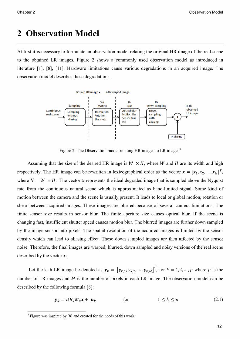
At first it is necessary to formulate an observation model relating the original HR image of the real scene
to the obtained LR images. Figure 2 shows a commonly used observation model as introduced in
literature [1], [8], [11]. Hardware limitations cause various degradations in an acquired image. The
observation model describes these degradations.
Figure 2: The Observation model relating HR images to LR images3
Assuming that the size of the desired HR image is � × �, where � and � are its width and high
respectively. The HR image can be rewritten in lexicographical order as the vector � = [�, ��, … , � ]�,
where � = � × �. The vector � represents the ideal degraded image that is sampled above the Nyquist
rate from the continuous natural scene which is approximated as band-limited signal. Some kind of
motion between the camera and the scene is usually present. It leads to local or global motion, rotation or
shear between acquired images. These images are blurred because of several camera limitations. The
finite sensor size results in sensor blur. The finite aperture size causes optical blur. If the scene is
changing fast, insufficient shutter speed causes motion blur. The blurred images are further down sampled
by the image sensor into pixels. The spatial resolution of the acquired images is limited by the sensor
density which can lead to aliasing effect. These down sampled images are then affected by the sensor
noise. Therefore, the final images are warped, blurred, down sampled and noisy versions of the real scene
described by the vector�.
Let the k-th LR image be denoted as �� = ���,, ��,�, … , ��,���, for � = 1,2, … , � where � is the
number of LR images and � is the number of pixels in each LR image. The observation model can be
described by the following formula [8]:
�� = ������ + � for 1 ≤ � ≤ � (2.1)
3 Figure was inspired by [8] and created for the needs of this work.

Chapter 2 Observation Model
13
�� is a matrix representing the motion model, �� is a blur matrix, � represents a sub sampling matrix and � is a noise vector. The size of LR images is assumed to be the same, but in more general cases,
different sub sampling matrices (e.g.,��) can be used to address the different sizes of the LR images.
The linear system (2.1) expresses the relationship between the LR images and the desired HR image.
Super-resolution methods are able to solve the inverse problem and estimate the HR image. ��, ��, ��
matrices are unknown in real applications and it is necessary to estimate them from available LR images.
The linear system is ill-posed. Therefore, proper prior regularization is required. Chapter 4 presents
different methods to achieve it.

Chapter 3 Motion Estimation and Registration
14
3 Motion Estimation and Registration
Some works about SR simply skip the motion estimation (ME) problem, assuming that it is known, and
start from the frame fusion process. Synthetic data made under defined conditions sets a convenient
background for theoretical analysis and development of algorithms, but for real applications motion
estimation process has to be taken into account. In practice, input images for SR are obtained from the
video sequence. The LR video frames contain relative motion due to camera shift and also the changes in
the scene. Therefore, it is necessary to estimate motion and perform the registration step at the beginning
of each of the following SR techniques. Precision of the motion estimation is crucial for the success of the
whole SR reconstruction. If the images are badly registered, it is better to perform single LR image
interpolation than SR reconstruction using several LR images [4].
Motion estimation analyses successive images from a video sequence and determines
two-dimensional motion vectors describing the motion of objects from one image to another. Estimated
motion can be used for image registration. Image registration is a process of aligning two or more images
into a coordinate system of a reference image. Several surveys of image registration methods have been
developed [13], [14]. There are two main ME approaches – feature based and intensity based.
Feature based methods
Feature points are found by, for example, Harris or Hessian detector. Next step establish a
correspondence between pairs of selected feature points in two images and then transformation describing
the motion model between these images is computed. Feature points based methods are often used for
image stitching and object tracking applications.
Intensity based methods
The constant intensity assumption is used. It says that the observed brightness of an object is constant
over time [33]. Motion estimation is then performed as an optimization problem where different
estimation criteria can be used. Several main methods are discussed below.
Assuming two images shifted by a motion vector " = �"#, "$��. If the motion model is a pure
translation (camera is moving, scene is stationary), it can be expressed as:
%&�, �' = (&� + "#, � +"$' (3.1)
where % is the template (the reference image) and ( refers to the shifted image.
Chapter 3 Motion Estimation and Registration
15
Block matching techniques [16], [17] are widely used to estimate the parameters "#, "$. It consists of
computing the differences in intensity between blocks of pixels in the template and the shifted image. It
can be written as
)&", "�' = **[+(,� + "#, � + "$- − %&�, �'+]/ $0
�#0 (3.2)
where " is the displacement between the reference image % and the shifted image (, � and � are given
by the size of region where )&", "�' is calculated. When � = 1, the error )&", "�' is called the mean
absolute difference (MAD), when � = 2, it is called the mean square error (MSE) [33].
The error function described by equation (3.2) can be minimized by different algorithms such as
exhaustive search, gradient-based algorithm, three step search, 2D log search [33].
The normalized cross-correlation (NCC) is widely used matching method, particularly suitable for
translationally shifted images. One of the drawbacks of NCC is that its precision is limited to a pixel, but
a number of techniques have been used to achieve sub pixel precision [20]. The input image or the cross-
correlation surface can be interpolated to higher resolution and the peak is then relocated into the more
precise position. Another way to achieve sub pixel accuracy is to fit a continuous function to samples of
the discrete correlation data. Then a search for the maximum of this function is performed and more
precise location of the peak is found. The issue is to find a function well describing the cross-correlation
surface. However, the correlation surface around its peak often approaches to a bell shape [20]. When the
images are sampled at high enough frequency, the corresponding correlation function is quite smooth and
the surface can be approximated by second-order polynomial functions with accurate results [21].
Correlation is simple in principle. It searches a location of the best match between an image and a
template image. This approach becomes computationally intensive in the case of large images. Therefore,
an alternative approach is to implement correlation in the frequency domain which leads to the phase
correlation method (PCM). PCM is based on Fourier shift property which states that a shift in coordinate
frames of two functions is transformed in the Fourier domain as the linear phase difference [3]. PCM
computes a phase difference map that (ideally) contains a single peak. The location of the peak is
proportional to the relative shift between the two images [22].
Two images (&�, �', (�&�, �' are relatively shifted by a motion vector " = �"#, "$��. Let the
situation be described by equation (3.3).
(�&�, �' = (&� − "#, � − "$' (3.3)
Chapter 3 Motion Estimation and Registration
16
According to the Fourier shift property
1�2 &3, 4' = 12&3, 4'exp&−i,u"# + 4"$-' (3.4)
where 12&3, 4', 1�2&3, 4' denote the discrete Fourier transforms (DFT) of the images (&�, �', (�&�, �'. The normalized cross-power spectrum is given by
exp&−i,u"# + 4"$-' = 1�2&3, 4'12&3, 4'∗+1�2&3, 4'12&3, 4'∗+ (3.5)
where ∗ indicates the complex conjugate [3]. The inverse DFT is applied to normalized cross-power
spectrum and the result is ;,� − "#, � −"$- which is a Dirac delta function centered at &"#, "$'. PCM is robust to noise and image defects and it is much faster compared to the correlation in the
spatial domain. Thus, the phase correlation method is popular for image registration and many algorithms
were proposed to extend it to sub pixel accuracy. In the literature [22], three sub pixel PCM algorithms
were compared using a test set of realistic satellite images. Guizar et al. algorithm [23] performed the best
of these three investigated algorithms. [23] shows improvements based on nonlinear optimization and
discrete Fourier transform. It leads to shorter computational times and reduction of memory requirements.
When scenes contain moving objects, analysis is more complex. It is convenient to describe each
pixel by motion vector, representing the displacement of that point across two successive images. It
produces a dense motion field. The pattern of apparent motion of objects, surfaces, and edges in a visual
scene caused by the relative motion between a camera and the scene is called optical flow. Differential
methods use local Taylor series approximation of the image signal to calculate the optical flow for each
pixel. Intensity of a pixel in the image at the time t is defined as (&�, �, <'. The pixel has moved by "�, "�
in time "< between two successive image frames such that
(&�, �, <' = (&� + "�, � + "�, < + "<' (3.6)
Assuming the movement to be small, the intensity function (&�, �, <' can be expanded in a Taylor series:
(&� + "�, � + "�, < + "<' = (&�, �, <' + =(=� "� + =(=� "� +=(=< "<+. .. (3.7)
where the higher order terms have been ignored.
From equations (3.6) and (3.7) follows that:
=(=� "�"< + =(=� "�"< +=(=< "<"< = 0 (3.8)

Chapter 3 Motion Estimation and Registration
17
Equation (3.8) results in:
(#4# +($4$ = −(@ (3.9)
In equation (3.9), (#, ($, and (@ denote respective partial derivatives with respect to �, �, and <. The �
and � components of the velocity or optical flow are 4# and 4$. This equation does not enable to
determine a unique motion vector, because at each pixel there is only one scalar constraint and will not
suffice for determining the two components of the motion vector [4#, 4$]. Another set of equations is
needed to find the optical flow. It is achieved by introducing additional constraints. Horn-Schunck
method adds additional smoothness constraint to the optical flow constraint and iteratively minimizes the
total error [40]. Lucas-Kanade method [41] considers that the neighboring points of the pixel of interest
have the same apparent motion [4#, 4$]. The local motion vector have to satisfy:
(#&�'4# +($&�'4$ =−(@&�'(#&��'4# +($&��'4$ =−(@&��'⋮(#&�B'4# +($&�B'4$ =−(@&�B' (3.10)
where �, ��, … , �Bare the pixels inside the window. (#&�C', ($&�C', (@&�C' are the partial derivatives with
respect to �, �, and time < evaluated at the point &�C' at the time <. With for example 5x5 window 25
equations per pixel are obtained. The equations (3.10) can be rewritten in the matrix form D4 = E, where
D = FGGH(#&�' ($&�'(#&��' ($&��'⋮(#&�B' ⋮($&�B'IJ
JK , 4 = L4#4$M , E = −N(@&�'(@&��'⋮(@&�B'O (3.11)
The system has more equations than unknowns and is over-determined. The solution is obtained
using the least squares principle. Hence, D�D4 = D�E and next 4 = &D�D'PD�E. The motion vector
can be expressed as:
L4#4$M = FGGGGH *(#&�C'�B
C0 *(#BC0 &�C'($&�C'
*(#BC0 &�C'($&�C' *($&�C'�B
C0 IJJJJKP
FGGGGH−*(#B
C0 &�C'(@&�C'−*($B
C0 &�C'(@&�C'IJJJJK (3.12)
It should be stated that there are still a few problems with this method. Edges parallel to the
direction of motion would not provide useful information about the motion. In addition, regions of
constant intensity will have ∇( = 0, so (@ will be zero. Only edges with a component normal to the
direction of motion provide information about the motion [42].

Chapter 4 Super-resolution Image Reconstruction Techniques
18
4 Super-Resolution Image Reconstruction
Techniques
SR methods can be divided into four main groups: non-uniform interpolation approach in the spatial
domain, frequency domain approach, statistical approaches and other approaches (such as iterative back
projection and projection onto convex sets). Further in this chapter, theoretical basis of these approaches
are presented.
4.1 Non-Uniform Interpolation Approach
The algorithm is composed of three main stages as Figure 3 shows. Firstly, relative motion estimation
between observed LR images is performed. This part is often called registration and it is crucial for
success of the whole method. The estimation of relative shifts must have sub pixel precision. It has been
proved that 0.2 px precision of estimation is acceptable [12]. Pixels from registered LR images are
aligned in an HR grid. After this process, points in the HR grid are non-uniformly spaced and therefore
non-uniform interpolation is applied to produce an image with the enhanced resolution (HR image).
When the HR image is obtained, the restoration follows to remove blurring and noise. This approach is
simple and computationally efficient.
Figure 3: Non-uniform interpolation approach4
When LR images are aligned, a non-uniform interpolation is necessary to create a regularly sampled
HR image. The basic, very simple method is the nearest neighbor interpolation. For each point in the HR
grid, algorithm searches for a nearest pixel among all pixels which were aligned in the HR grid from LR
images (as Figure 1 shows). The nearest pixel value is then used for the current HR grid point.
Another often used and simple method is the bilinear interpolation. At first the nearest pixel is found
as in the previous case. The algorithm detects which LR image this pixel comes from and then picks up
three other neighboring pixels from the same LR image. The situation is described in Figure 4. The HR
4 Figure was inspired by [8] and created for the needs of this work.

Chapter 4 Super-resolution Image Reconstruction Techniques
19
grid point is surrounded by four LR pixels. These four pixels form a square so that the unknown value of
the HR grid point can be calculated using the bilinear weighted sum. Similarly, the bicubic interpolation
can be applied if 16 pixels in the LR image are selected (instead of four). These two methods are
efficiently fast, but there is a disadvantage. Some of the 4 pixels (or 16 pixels) used for the interpolation
are not among the 4 (or 16) absolutely closest pixels from all LR images. The situation is demonstrated in
Figure 4. Some other pixels from other LR image are in fact closer to the HR grid point. Therefore, they
may contain more relevant information about the unknown HR grid point value. Other methods are based
on a selection of four closest pixels from all pixels from all input LR images (not only from a single LR
image). A question remains in the determination of the weights for each of these pixels. The weights can
be simply determined by a function of distance between the LR image pixel and the HR grid point.
Figure 4: Bilinear non-uniform interpolation and near optimal non-uniform interpolation5
Gilman and Bailey introduced near optimal non-uniform interpolation [25]. They assume that the
optimal weights depend only weakly on the image content and mostly on the relative positions of the
available samples. Therefore, the weights derived from a synthetic image can be applied to the input LR
images with the same offsets. In other words, an arbitrary HR image is used to generate synthetic LR
images with the same properties (size, shifts, blur) as the input LR images. The values of the weights are
then derived to minimize the mean squared error between the auxiliary HR image and its version restored
from the synthetic LR images.The near optimal interpolation method provides good results, but the
computational cost rises rapidly if the motion model between the LR images is more complex than global
5 Figure was inspired by [1] and created for the needs of this work.

Chapter 4 Super-resolution Image Reconstruction Techniques
20
translation. As a result the near optimal interpolation method as well as the bilinear interpolation method
is suitable only in case of a global, pure translational movement.
Lertrattanapanich and Bose used Delaunay triangulation and then fit a plane to each triangle to interpolate
an HR grid point inside the triangle [24].
The last part contains deblurring and noise removal. Restoration can be performed by applying any
deconvolution method that considers the presence of noise. Wiener filtering is widely used. There is a
huge amount of works dedicated to image enhancement [33],[34], but that is not directly connected to SR
techniques. Thus, it is not discussed here in details.
4.2 Frequency Domain Approach
The frequency domain approach introduced by Tsai and Huang [26] is based on the following three
principles: 1) the assumption that the original HR image is band limited, 2) the shifting property of the
Fourier transform, 3) the aliasing relationship between the continuous Fourier transform of the original
HR image and the discrete Fourier transform of observed LR images [8].
These principles allow formulating the system of equations and reconstructing the HR image using
the aliasing that exists in each LR image. Let �&<, <�'be a continuous image and ��&<, <�' � = 1,2, … , � be a set of� spatially shifted versions of �&<, <�'. Then
�&<, <�' = ��&< +R# , <� +R$', (4.1)
where ∆x, ∆y are arbitrary but known shifts of �&<, <�'along the � and � coordinates, respectively. The
continuous Fourier transform (CFT) is applied to both sides of the equation and by the shifting properties
of the CFT, we obtain:
S�&3, 3�' = TU�V,WXYZ[W\Y]-S&3, 3�'. (4.2)
The shifted images��&< +R#, <� +R$' are sampled with the sampling period %and %� and LR
images are generated ��&^, ^�' = ��,^% +R#, ^�%� +R$-with ^ = 0,1,2, … ,� − 1 and ^� = 0,1,2, … ,�� − 1. Denote the discrete Fourier transform (DFT) of these LR images by _�[ ̀, �̀]. Assuming the band limitedness ofS�&3, 3�', |S�&3, 3�'| = 0for |3| ≥ &�c'/%, |3�| ≥ &��c'/%�. The relationship between the CFT of the HR image and the DFT of the k-th observed
LR image can be written as [8]:
_�& ̀, �̀' = 1%%� * * S� e2c% f ̀� −gh , 2c%� f �̀�� −g�hi ]Pj]kl
ZPjZkl
(4.3)
Chapter 4 Super-resolution Image Reconstruction Techniques
21
The matrix vector form is obtained as:
_ = mS , (4.4)
where _ is a � × 1 column vector with the k-th element of the of the DFT coefficient _�& ̀, �̀', S is a ��� × 1 column vector with the samples of the unknown CFT coefficients of �&<, <�', and m is a � ×��� which relates the DFT of the LR images to the samples of the continuous HR image.
The reconstruction of a desired HR image requires to determine m and then to solve the set of linear
equations (4.4). S is obtained and the inverse DFT is applied to get the reconstructed image. Many
extensions to this approach have been provided considering different blur for LR images [27], reducing
the effects of registration errors [31], reducing memory requirements and computational cost [32].
However, the frequency approach is limited in principle by its initial condition. The observation model is
restricted to the global translational motion only. More complicated motion models cannot be used.
Although this approach is computationally efficient and simple in theory, later works about SR have been
devoted mainly on the spatial domain.
4.3 Regularized SR Reconstruction
The observation model (2.1) described in the second chapter can be also expressed as:
�� = ��� + � for 1 ≤ � ≤ � , (4.5)
where �� is a matrix which represents down sampling, warping and blur. The linear system (4.5) has to
be solved to reconstruct an HR image. The SR problem can be defined as the inversion of the system
(4.5), where � is the additive noise. If the ��P is applied to equation (4.5), it leads to: ��P�� = � +��P �. It would cause amplification of the noise. In the presence of noise the inversion
of the system becomes unstable. SR reconstruction is generally an ill-posted problem and some
regularization is necessary. It means the need of adding a constraint which stabilizes the inversion of the
system and ensures the uniqueness of the solution. Deterministic and stochastic regularization approaches
are further described.
4.3.1 Deterministic Approach
There are many standard techniques how to impose prior information of the solution space in order to
regularize the SR problem. Perhaps the most common one uses a smoothness constraint and a least
squares optimization [27]. A smoothness constraint is derived from the assumption that most images are
naturally smooth with limited high-frequency information. Therefore, it is appropriate to minimize the
amount of high-pass energy in the restored HR image [8].

Chapter 4 Super-resolution Image Reconstruction Techniques
22
Assuming the matrix �� in equation (4.5) can be estimated for each input LR image �� , the HR
image can be reconstructed by minimizing the following function
1&�' = *‖�� −���‖� + o‖p�‖q�0 (4.6)
with p a matrix which represents a high pass filter, o is a regularization parameter controlling the tradeoff
between the fidelity of the data and the smoothness of the HR estimate. In other words, o controls how
much weight is given to the regularization constraint. Larger values of o usually lead to a smoother HR
image[8]. The cost function with regularization term is convex and differentiable. It can be found a
unique estimate of the HR image � minimizing the cost function (4.6).
4.3.2 Stochastic Approach
Statistical approaches give another way to handle prior information and noise. If the a posteriori
probability density function (PDF) of the original image can be established, the Bayesian approach is
commonly used [8]. Using the Bayesian approach, the HR image and motions among LR input images
are regarded as stochastic variables to which probability distributions can be associated. Stochastic
approach encompasses maximum likelihood (ML) and maximum a posteriori (MAP) estimation
techniques. Maximum likelihood estimation (i.e., a special case of MAP estimation with no prior
knowledge) can also be applied, but because the SR inverse problem is ill-posed, MAP estimation is
usually preferred. In the observation model (4.5), the LR images �� , noise � and the HR image � are
assumed to be stochastic and the matrix �� is known.
Schultz and Stevenson [28] introduced the MAP technique for SR reconstruction. The algorithm
searches for an HR image � that maximizes the probability that the HR image is represented by observed
LR images.
�r = argmax�w,�|�x, �y, … , �z-� (4.7)
Applying the Bayes's theorem to the conditional probability and taking the logarithm of the result, we
obtain:
�r = argmax�log w,�x, �y, … , �z+�- + log w&�'�. (4.8)
Hence, the prior image density w&�' and the conditional density w,�x, �y, … , �z+�- have to be specified.
It can be defined by a priori estimate of HR image � and the statistical information of noise.

Chapter 4 Super-resolution Image Reconstruction Techniques
23
The LR images �� are independent as well as the noise process �. It can be written:
w,�x, �y, … , �z+�- = }w&��|�'z�0x (4.9)
Additive noise in the equation (4.5) is usually modeled by a zero-mean and white Gaussian noise with
variance ~�. Therefore, equation (4.5) can be expressed as a density function [1]:
w&��|�' ∝ exp �−‖�� −���‖y2~� � (4.10)
Prior information about the HR image can be modeled by Markov random field (MRF). w&�' is usually
defined using the Gibbs distribution in an exponential form:
w&�' = 1� exp �−*��&�'�∈� � (4.11)
where Z is a normalizing constant, �� is the clique potential and p is the set of all cliques in the image [2].
In order to apply fast minimization technique it is important to have a complex energy function, so that
the minimization process will not stop in local minima. To impose the smoothness condition to the HR
image, a quadratic cost can be considered. It is a function of finite difference approximations of the first
order derivative at each pixel location [2]. It leads to the expression:
��&�' = 1o**L,�&�, �' − �&�, � − 1'-� + ,�&�, �' − �&� − 1, �'-�M U0
�C0 (4.12)
where λ is a constant defining the strength of the smoothness assumption.
From the equations (4.8) and (4.9):
�r = argmax �log}w&��|�'z�0x +log w&�'�
�r = argmax �* logw&��|�'/�0 +log w&�'�
(4.13)
Chapter 4 Super-resolution Image Reconstruction Techniques
24
Substituting equations (4.10) and (4.11) into equation (4.13) we obtain:
�r = argmax �*−‖�� −���‖y2~�/
�0 −*��&�'�∈� ��r = argmin �*‖�� −���‖y2~�
/�0 +*��&�'�∈� �
(4.14)
The equation above can be simply minimized by gradient descent optimization. The cost function of the
equation (4.14) consists of two terms. The first one describes the error between the estimated HR image
and the observed LR images.. The second part is the regularization term which contribution is controlled
by the parameter. The gradient of (4.14) at the nth iteration is given by:
�&B' = 1~�*���,���&B' − ��-/�0 + �&B'o
(4.15)
where �&B'at the location &�, �' in the SR grid is defined as:
�&B'&�, �' = 2�4�&B'&�, �' − �&B'&�, � − 1' − �&B'&�, � + 1' − �&B'&� − 1, �' − �&B'&� + 1, �'�. (4.16)
The estimate at &^ + 1'@� iteration can be obtained as:
�&B[' = �&B' − ��&B' (4.17)
where αis the step size. Computation iteratively continues until ��&B[' −�&B'� < threshold. Bilinear
interpolation of the least blurred LR image can be used as the initial estimate [2].
4.4 Other Super-Resolution Approaches
4.4.1 Projection onto Convex Sets
The projection onto convex sets (POCS) is another iterative method which employs prior knowledge of
the solution. Each LR image defines a constraining convex set of possible HR images. When the convex
sets are defined for all LR images, an iterative algorithm is employed to an intersection of the convex
sets. We assume that HR image belongs to this intersection. The POCS technique uses the following
algorithm (11) to find a point within the intersection set given by an initial guess [1]:
��[x = w�w�P…w�w�� , (4.18)
where ��is an initial guess, wU is the projection of a given point onto the j-th convex set an M is the
number of convex sets.

Chapter 4 Super-resolution Image Reconstruction Techniques
25
4.4.2 Iterative Back-Projection
The algorithm based on iterative back projection (IBP) was introduced by Irani and Peleg [30]. The key
idea is simple. First HR image is estimated and then LR images are synthetically formed from this HR
image according to the observation model. The HR image is iteratively refined by back projecting the
error (i.e., the difference) between synthetically formed LR images and observed LR images until the
energy of the error is minimized. The back projection function is defined as:
�&B[' =�&B' + �*��P�ℎ�/� ∗ ↑ &�r� −��'�� (4.19)
where c is constant, ℎ�/� is the back-projection kernel, ↑ is the up sampling operator and �¢� is the
simulated k-th LR image from the current HR image estimate. The algorithm is relatively simple and able
to handle many observations with different degradations. However, the solution of back projection is not
unique. It depends on the initialization and choice of the back projection kernel. The back projection
method is nothing else than an ML estimator [1].

Chapter 5 Experimental Part: Image Processing
26
5 Experimental Part: Image Processing
The aim of the work is to find an optimal SR method applicable to real video sequences from different
domains such as satellite, microscopy or thermal imaging, forensic applications etc. Therefore, the
resulting algorithm should be reasonably quick and able to process a large number of color images (video
sequences). Further it should achieve very good image quality of the output under different circumstances
(different motion model, scene etc.), so versatility is advisable.
Non-uniform interpolation approach seems to be suitable to tackle with this task because of its
relatively simple implementation, versatility and calculation speed. Statistical approaches are
computationally more demanding, but they have potential to provide very good image quality.
In this work, eight SR reconstruction algorithms and five algorithms for motion estimation were
programed. PSNR and MSSIM are often used for objective evaluation of SR methods [24],[43],[44],[46].
Therefore, these measurements were used also in this work. The further part of the work is devoted to the
examination of objective and subjective quality and computational complexity of the SR methods. Firstly,
implemented algorithms are compared by their subjective image quality, PSNR, MSSIM and processing
time. Secondly, programmed motion estimation algorithms (essential for image registration) are presented
and their accuracy and speed compared. In the chapter 6, the most suitable combination of motion
estimation and SR reconstruction are applied to real color video sequences.
5.1 Non-Uniform Interpolation Approach: Interpolation
Nine interpolation methods were implemented in MATLAB R2012a. To evaluate their performance, the
function createDataset1.m was programmed. This function creates an artificial dataset of mutually
shifted images by different random sub pixel shifts from an arbitrary input image. The number of LR
images required can be specified, as well as the decimation factor, which defines how many times the LR
images will be smaller than the input image. First reference image is created, then blurs due to the optics
and due to the integration on the sensor are simulated using Gaussian point spread function (PSF).
Gaussian PSF is the most common blur function of many optical imaging systems [43]. Next the input
image is randomly shifted in the range (-1,1) px with sub pixel precision and down sampled. This step
repeats until all LR images are obtained. As a result defined number of LR images is made with exactly
known shifts and the reference image. The reference image can be further use to compute objective
metrics such as PSNR and MSSIM.
Chapter 5 Experimental Part: Image Processing
27
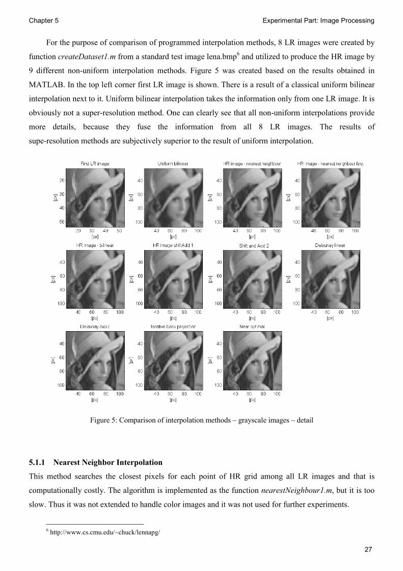
For the purpose of comparison of programmed interpolation methods, 8 LR images were created by
function createDataset1.m from a standard test image lena.bmp6 and utilized to produce the HR image by
9 different non-uniform interpolation methods. Figure 5 was created based on the results obtained in
MATLAB. In the top left corner first LR image is shown. There is a result of a classical uniform bilinear
interpolation next to it. Uniform bilinear interpolation takes the information only from one LR image. It is
obviously not a super-resolution method. One can clearly see that all non-uniform interpolations provide
more details, because they fuse the information from all 8 LR images. The results of
supe-resolution methods are subjectively superior to the result of uniform interpolation.
Figure 5: Comparison of interpolation methods – grayscale images – detail
5.1.1 Nearest Neighbor Interpolation
This method searches the closest pixels for each point of HR grid among all LR images and that is
computationally costly. The algorithm is implemented as the function nearestNeighbour1.m, but it is too
slow. Thus it was not extended to handle color images and it was not used for further experiments.
6 http://www.cs.cmu.edu/~chuck/lennapg/

Chapter 5 Experimental Part: Image Processing
28
If global motion is assumed, then each motion vector describing the motion between two images is
the same for all pixels of an image. In that case, the nearest neighbors can be computed only for a small
sample of an image and then applied to the whole part. This idea is programmed in the function
nearestNeighbour_fast.m. It is very quick, but the resulting HR image tends to be distorted if the shifts
between LR images lead to unequal distribution of pixels among the points of HR grid. Unequal
distribution means that some empty points of HR grid are surrounded by more pixels from LR images
then others. Algorithm nearestNeighbour_fast.m was not adopted for color images and was not used for
further work with video sequences.
Figure 6: Comparison of interpolation methods – RGB images – detail
5.1.2 Non-Uniform Bilinear Interpolation
The basic principle was described in the part 4.1. Algorithm is limited only to the global motion case, but
is reasonably quick due to the simplification of the model. HR grid points are calculated using the bilinear
weighted sum and it causes blurring as according image in Figure 6 demonstrates.
Chapter 5 Experimental Part: Image Processing
29
5.1.3 Shift and Add Interpolation
The algorithm takes all pixels of LR images, multiply their coordinates by super-resolution factor and
round them to the nearest integer so they can be easily placed in the HR grid. HR grid points which
remain empty need to be interpolated. Function nearestNeighbour_shiftAdd1.m fills the empty places by
nearest known points. Function nearestNeighbour_shiftAdd2.m counts weighted average of the nearest
known points.
More LR images cover more points of HR grid directly without additional interpolation. Thus the
algorithm provides better results when more LR images are at the disposal. Experiments showed that
super-resolution factor to the 3rd power it’s the number of LR images which provides good results.
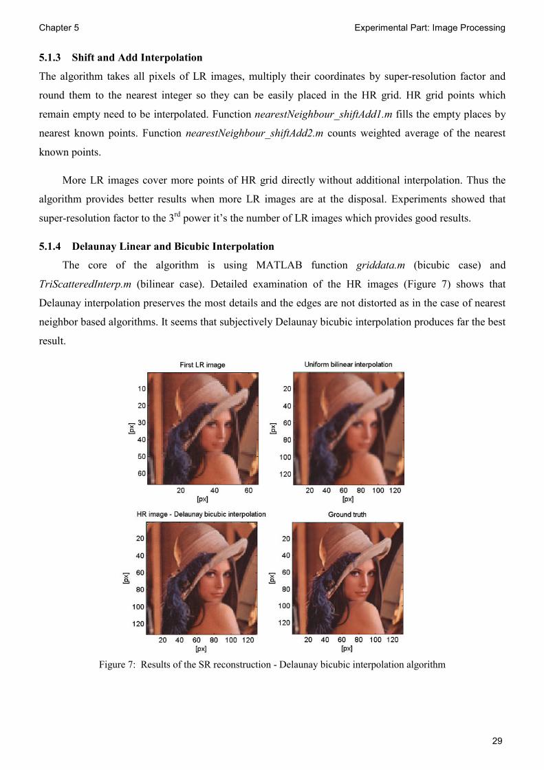
5.1.4 Delaunay Linear and Bicubic Interpolation
The core of the algorithm is using MATLAB function griddata.m (bicubic case) and
TriScatteredInterp.m (bilinear case). Detailed examination of the HR images (Figure 7) shows that
Delaunay interpolation preserves the most details and the edges are not distorted as in the case of nearest
neighbor based algorithms. It seems that subjectively Delaunay bicubic interpolation produces far the best
result.
Figure 7: Results of the SR reconstruction - Delaunay bicubic interpolation algorithm

Chapter 5 Experimental Part: Image Processing
30
5.1.5 Iterative Back Projection
The algorithm is iteratively trying to simulate the blurring and down sampling process when LR images
are produced. The algorithm was described in details in the section 4.4.2. The implemented algorithm
tends to sharpen too much the resulting HR image.
5.1.6 Near Optimal Interpolation
The algorithm described in the part 4.1 has promising results, but it is restricted to global motion only. If
the motion model would be more complex, the weights would have to be computed for each point of HR
grid independently. The computational load would be enormous. Further examination also revealed that
the implemented algorithm is very sensitive to errors in motion estimation.
5.1.7 Comparison by PSNR and MSSIM Evaluation
PSNR (Peak Signal to Noise Ratio) is commonly used metric for objective quality measurement. It is
calculated by the formula (5.1).
w �£ = 20 log f�DS¤√� )h (5.1)
�DS¤ is the maximum possible pixel value of the image. If the pixels are represented by 8 bits per sample
and the pixel values are represented from 0 to 255, �DS¤ equals 255.
MSE (Mean Square Error) is given by:
� ) = 1� 1�**&(¦§� − (̈ ©'� U0
�C0 (5.2)
where (¦§� is the reference image, (̈ © is the image created by SR method, � is the number of rows of the
image, � is the number of columns of the image.
The MATLAB code for MSSIM (Mean Structure Similarity Index) computation was downloaded
from the web page7 [38]. Firstly, SSIM is calculated for several regions (image patches) of the image and
then MSSIM is the mean of these values. The principle of SSIM is described in [39]. Suppose that � and � are local image patches taken from the same location of two images that are being compared. SSIM is
expressed as:
(�&�, �' = ,2μ#μ$ + p-&2~#$ + p�'&μ#� + μ$� + p'&~#� + ~$� + p�' (5.3)
7 www.ece.uwaterloo.ca
Chapter 5 Experimental Part: Image Processing
31
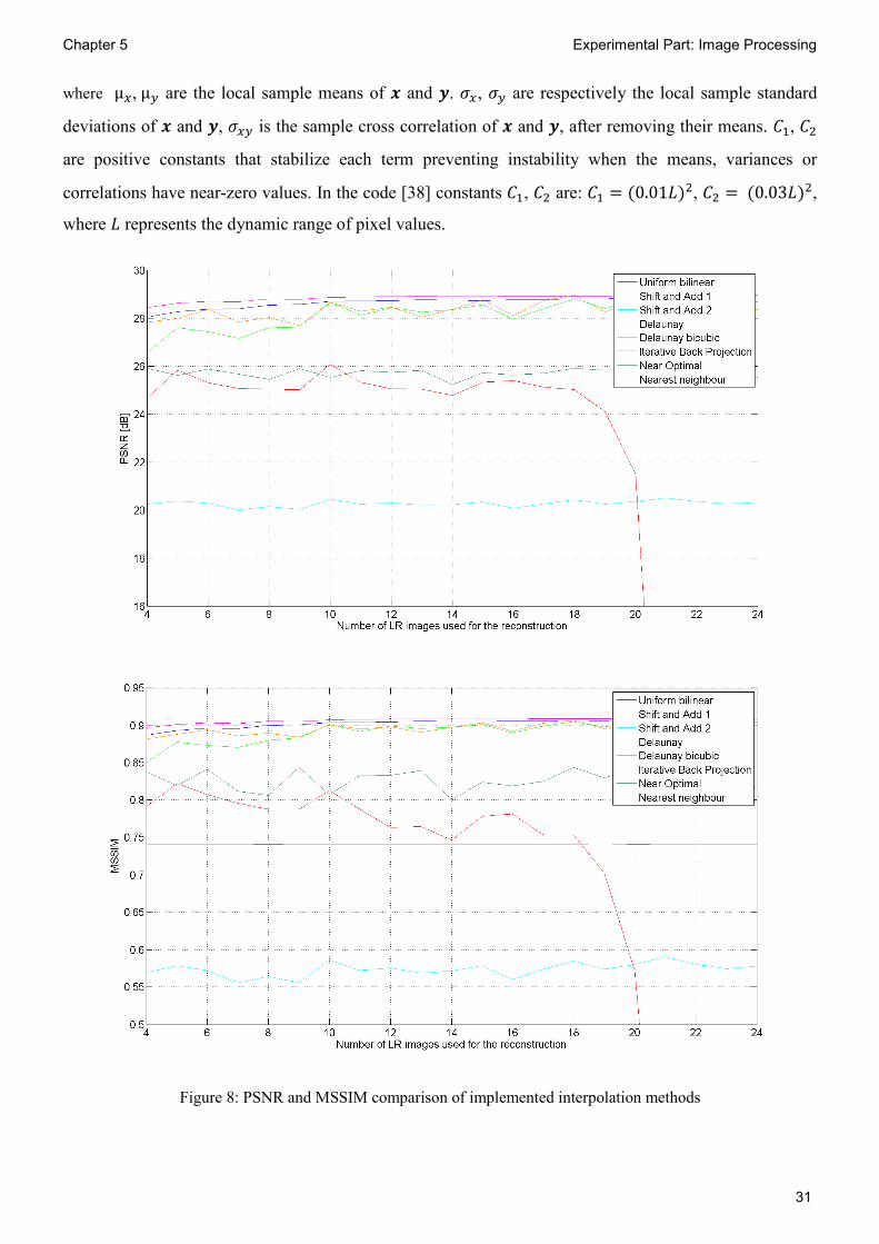
where μ#,μ$ are the local sample means of � and �. ~#, ~$ are respectively the local sample standard
deviations of � and �, ~#$ is the sample cross correlation of � and �, after removing their means. p, p�
are positive constants that stabilize each term preventing instability when the means, variances or
correlations have near-zero values. In the code [38] constants p, p� are: p = &0.01«'�, p� = &0.03«'�,
where « represents the dynamic range of pixel values.
Figure 8: PSNR and MSSIM comparison of implemented interpolation methods
Chapter 5 Experimental Part: Image Processing
32
PSNR and MSSIM metrics were calculated to provide objective comparison of the implemented
interpolation methods (Figure 8). For different number of LR images PSNR and MSSIM were measured
ten times (each time with different random shifts between LR images) and the values were averaged to
obtain more precise results. Super-resolution factor equals 2. Green line marks the uniform bilinear
interpolation. All SR methods performed better than uniform bilinear interpolation except one (light blue
line). PSNR and MSSIM have both similar characteristics. The highest PSNR and MSSIM are provided
by Delaunay bicubic interpolation. Since super-resolution factor equals 2, adding more than 8 LR images
do not improve PSNR very much. Only PSNR of nearestNeighbour_shiftAdd1.m algorithm rises
significantly with growing number of LR images. Iterative back projection algorithm has problems to
converge if more than 18 LR images are used. It is reflected by rapid decline of the PSNR and MSSIM
characteristic. On the contrary, processing time starts growing fast when algorithm fails to converge
quickly for more than 18 LR images (Figure 10).
Surprisingly nearestNeighbour_shiftAdd2.m algorithm has significantly lower PSNR and MSSIM
then simple uniform bilinear interpolation despite that the resulting HR image looks subjectively better.
The algorithm nearestNeighbour_shiftAdd2.m causes slight shift of HR grid points compared with the
initial LR image grid and as a consequence PSNR and MSSIM decrease rapidly. Figure 9 depicts the
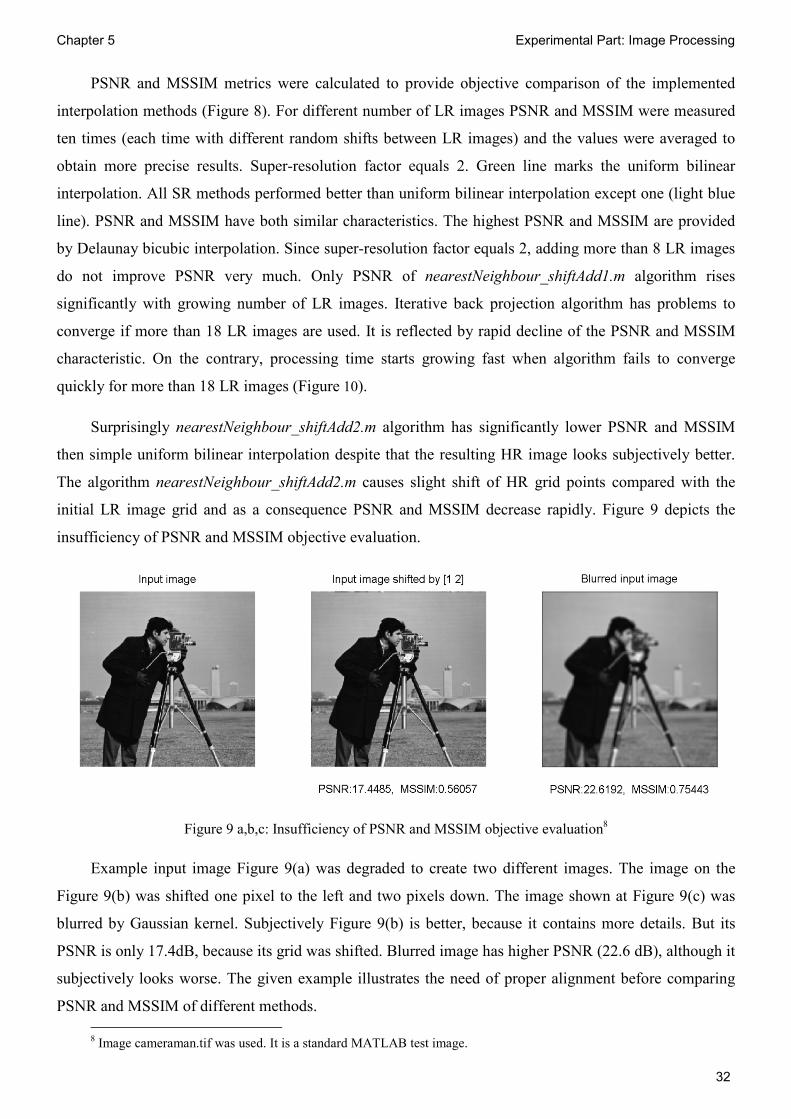
insufficiency of PSNR and MSSIM objective evaluation.
Figure 9 a,b,c: Insufficiency of PSNR and MSSIM objective evaluation8
Example input image Figure 9(a) was degraded to create two different images. The image on the
Figure 9(b) was shifted one pixel to the left and two pixels down. The image shown at Figure 9(c) was
blurred by Gaussian kernel. Subjectively Figure 9(b) is better, because it contains more details. But its
PSNR is only 17.4dB, because its grid was shifted. Blurred image has higher PSNR (22.6 dB), although it
subjectively looks worse. The given example illustrates the need of proper alignment before comparing
PSNR and MSSIM of different methods. 8 Image cameraman.tif was used. It is a standard MATLAB test image.
Chapter 5 Experimental Part: Image Processing
33
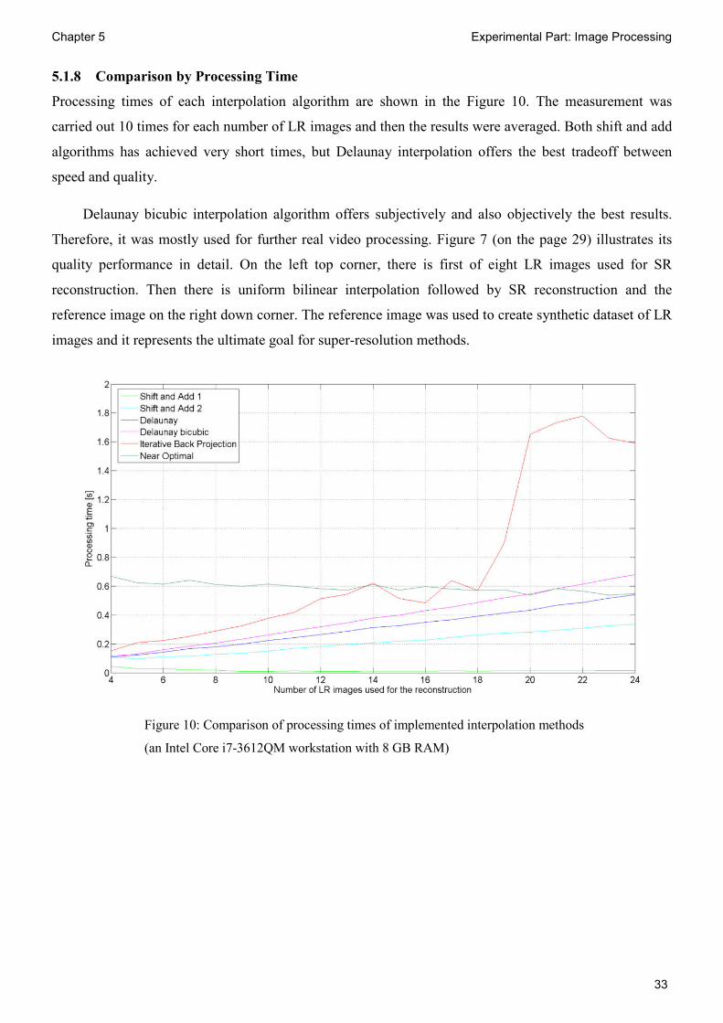
5.1.8 Comparison by Processing Time
Processing times of each interpolation algorithm are shown in the Figure 10. The measurement was
carried out 10 times for each number of LR images and then the results were averaged. Both shift and add
algorithms has achieved very short times, but Delaunay interpolation offers the best tradeoff between
speed and quality.
Delaunay bicubic interpolation algorithm offers subjectively and also objectively the best results.
Therefore, it was mostly used for further real video processing. Figure 7 (on the page 29) illustrates its
quality performance in detail. On the left top corner, there is first of eight LR images used for SR
reconstruction. Then there is uniform bilinear interpolation followed by SR reconstruction and the
reference image on the right down corner. The reference image was used to create synthetic dataset of LR
images and it represents the ultimate goal for super-resolution methods.
Figure 10: Comparison of processing times of implemented interpolation methods
(an Intel Core i7-3612QM workstation with 8 GB RAM)

Chapter 5 Experimental Part: Image Processing
34
5.2 Regularized SR Reconstruction
Regularized approach was investigated and an algorithm based on MAP estimation technique (described
in the part 4.3) was implemented in MATLAB. The algorithm (estimateMAP.m) was tested on the
synthetic dataset created by function createDatasetRGB2.m. The input image bfly.jpg9 was randomly
shifted with sub pixel precision, blurred by Gaussian blur (kernel size = 15px, sigma = 1.5px) and down
sampled to create desired number of LR images. Sixteen LR images were combined to reconstruct the HR
image with the up sampling factor 4 (see Figure 11). One of the LR images is shown in the top left corner
of Figure 11. It is followed by the results of Delaunay bicubic algorithm and MAP algorithm. For easier
comparison of the results, the ground truth (reference image) is shown in the right down corner. Both SR
methods provide more information about the high frequencies of the image. Parts of the structure of the
butterfly wings were not present in the LR image, or it was not possible to resolve them. It is clearly
visible, that MAP method enable to recover more details, then Delaunay bicubic algorithm. MAP
estimation method seems to have a great potential in image improvement. However its computational cost
is approximately 8 times (Table 1) higher compared to non-uniform algorithms presented in the previous
section.
Processing times were investigated using 3 different sets of LR images. Every time 16 LR images
were combined to produce the HR image with up sampling factor 4 (srFactor = 4). Each set of LR images
has different pixel size. It leads to the different pixel size of the final HR image (Table 1). Each
processing time is the average of 20 measurements. MAP estimation algorithm is approximately 8 times
slower which hampers its use for large video sequences. However, if the motion model is simplified this
approach can be effectively utilized even for real video sequence and provides very good results as
demonstrated in the section 6.3.
Table 1: Processing time comparison on an Intel Core i7-3612QM workstation with 8 GB RAM
Considering the speed, image improvements and objective evaluation. Delaunay bicubic algorithm
was chosen for further use for video sequences where the motion model is more complicated than the
pure translation. When the task requires to improve the resolution only for a small region of interest,
MAP estimation method is used providing the best image improvement.
9 Photography Randy L Emmitt (http://www.rlephoto.com/)
Method Time for HR image 176x176 px
Time for HR image 264x264 px
Time for HR image 528x528 px
Delaunay bilinear 0.59 1.22 5.01 Delaunay bicubic 0.60 1.30 5.30 MAP method 4.31 10.68 44.36

Chapter 5 Experimental Part: Image Processing
35
Figure 11: The results of SR reconstruction – comparison between Delaunay interpolation
and MAP estimation method, 16 LR images were combined, srFactor = 4
5.3 Registration: Motion Estimation
In the previous section interpolation algorithms were examined using artificial dataset with known shifts.
That is satisfactory for evaluation purposes in laboratory conditions, but in the real situation motions
between LR images have to be estimated. Precision of the estimation has the major effect on the final HR
image. If the motion estimation is not precise, the overall super-resolution method is unsuccessful.
5.3.1 Motion Models
Motion estimation from intensity values obtained from the images is a complex problem for many
reasons. The real scene is three dimensional, but images are only a 2D representation. Consequently,
motion estimation methods have to rely on the apparent motion of the objects relative to the image.

Chapter 5 Experimental Part: Image Processing
36
Relative motion between the camera and the scene can be very complex. If the camera is moving,
different objects are quickly moving in the scene and also background is changing in the same time. Then
motion estimation is extremely challenging task and beyond the reach of contemporary computer vision
solutions [33]. But if some constraints are introduced, difficult complex model is simplified and motion
estimation may be performed.
In purpose of this work three different cases of relative movements between camera, objects of
interest, and background were assumed:
1. Global motion
2. Different local motions
3. The use of a region of interest only
The simplification makes the motion estimation possible, yet it is a suitable description for many real
video sequences.
Global motion
In this case, camera is shifting in one plane, but objects are fixed and background is constant. All pixels
are moving in the same direction, so each of them has the same motion vector. The motion between two
successive frames can be described by one motion vector only and that simplifies the computation hugely.
The result of simplification forms a good model for real situations like for example video from a satellite
orbiting Earth or shifting sample observed by a microscope.
Different local motion
Camera is still, single or several objects are moving, background is constant. The typical example is a car
moving across the street recorded by a security camera.
The use of a region of interest only
More complex model can be converted to the global motion case mentioned earlier if only a small region
of interest (ROI) is taken from the sequence. ROI has to be marked, tracked and cut from an each image
of the video sequence.
Five different estimation algorithms were programmed in MATLAB and their performance
evaluated. These algorithms are based on three theoretical principles described in the chapter 3.
1. Block matching
2. Normalized cross correlation
3. Optical flow

Chapter 5 Experimental Part: Image Processing
37
Classical block matching algorithm is very simple in principle and can provide fine results, but
interpolation is necessary to obtain sub pixel precision. The original image has to be interpolated on 10
times larger grid to obtain the theoretical precision 0.1 px. If the precision 0.05 is demanded, then the
image has to be interpolated by factor 20 etc. Computational time raises rapidly with the higher precision.
Typical block matching algorithm using MSE calculation was implemented in MATLAB function
blockMatching.m.
The algorithm called ccrShiftEstimation.m is based on the normalized cross correlation. The
algorithm provides results with good precision. Interpolation is also necessary for sub pixel precision, but
computation in the frequency domain is quicker, so the tradeoff between precision and speed is better
than in the case of blockMatching.m. If only global motion model is assumed the algorithms mentioned
above work well and the simplicity of the model brings the possibility to calculate cross correlation only
in the main part of the image (not whole). This modification is reflected in the function
ccrShiftEstimation_fast.m which allows further speed performance improvement.
In the case of local motion, each pixel may have a little different motion vector. Therefore, it is
necessary to perform motion estimation for each pixel. Previous algorithms could be theoretically
adjusted to solve the problem, but it would be computationally very demanding. Optical flow based
algorithms seems to be more suitable for application on the local motion model. Optical flow algorithm
based on the Lucas Kanade theory [41] was implemented in the function optFlow_LK.m. The precision is
sufficient, but there is inherent ambiguity in the motion estimation process based on the edges of the
objects within the frame. That is known as aperture problem [33]. Figure 12 illustrates the situation.
Figure 12: The aperture problem
The edge in Figure 12 is observed through a small circular aperture. The task is to estimate motion
of the point X which position is given by xi and yi coordinates. Optical flow based methods use motion
vector perpendicular to the edge to estimate the motion. In Figure 12 it would be motion to the right and
up. In fact it is not possible to decide if the edge has not moved purely to the right or even purely up.
Chapter 5 Experimental Part: Image Processing
38
Aperture problem limits the maximum shift between the object in two consecutive frames. If the shift is
large too much, the motion estimation fails. Function optFlow_LK_pyramid.m uses the hierarchical
system described in [29],[33]. Robustness is improved and larger shifts are detectable.
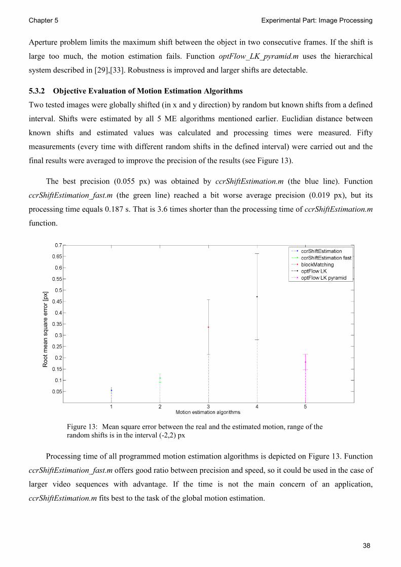
5.3.2 Objective Evaluation of Motion Estimation Algorithms
Two tested images were globally shifted (in x and y direction) by random but known shifts from a defined
interval. Shifts were estimated by all 5 ME algorithms mentioned earlier. Euclidian distance between
known shifts and estimated values was calculated and processing times were measured. Fifty
measurements (every time with different random shifts in the defined interval) were carried out and the
final results were averaged to improve the precision of the results (see Figure 13).
The best precision (0.055 px) was obtained by ccrShiftEstimation.m (the blue line). Function
ccrShiftEstimation_fast.m (the green line) reached a bit worse average precision (0.019 px), but its
processing time equals 0.187 s. That is 3.6 times shorter than the processing time of ccrShiftEstimation.m
function.
Figure 13: Mean square error between the real and the estimated motion, range of the random shifts is in the interval (-2,2) px
Processing time of all programmed motion estimation algorithms is depicted on Figure 13. Function
ccrShiftEstimation_fast.m offers good ratio between precision and speed, so it could be used in the case of
larger video sequences with advantage. If the time is not the main concern of an application,
ccrShiftEstimation.m fits best to the task of the global motion estimation.
Root mean square error [px]
Chapter 5 Experimental Part: Image Processing
39
Table 2: Processing times of different motion estimation algorithms on an Intel Core
i7 3612QM workstation with 8 GB RAM
Algorithm Processing time [s] ccrShiftEstimation 0.68 ccrShiftEstimation fast 0.19 blockMatching 0.74 optFlow LK 1.38 optFlow LK pyramid 1.59
For local motions, these algorithms are not suitable. If the video sequence with local motions is
processed, there are two algorithms to choose from - optFlow_LK.m and optFlow_LK_pyramid.m. The
latter is slower, but it achieves higher precision and it is more robust to larger shifts. The precision of
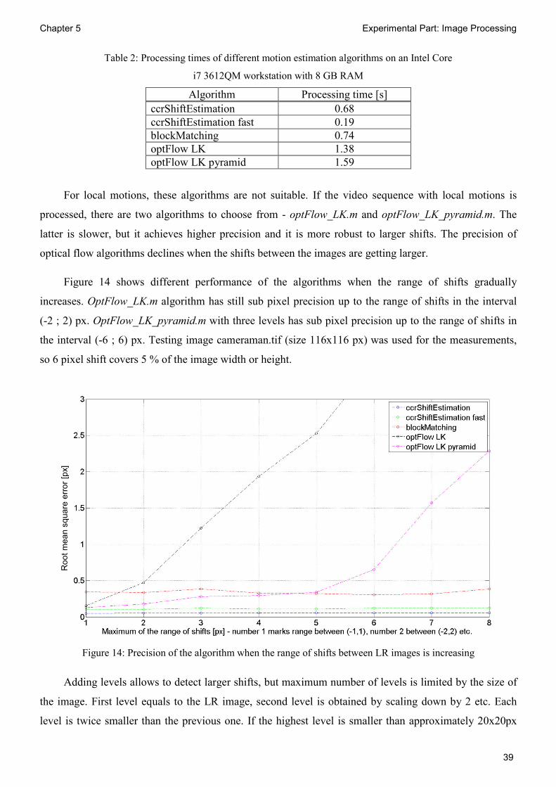
optical flow algorithms declines when the shifts between the images are getting larger.
Figure 14 shows different performance of the algorithms when the range of shifts gradually
increases. OptFlow_LK.m algorithm has still sub pixel precision up to the range of shifts in the interval
(-2 ; 2) px. OptFlow_LK_pyramid.m with three levels has sub pixel precision up to the range of shifts in
the interval (-6 ; 6) px. Testing image cameraman.tif (size 116x116 px) was used for the measurements,
so 6 pixel shift covers 5 % of the image width or height.
Figure 14: Precision of the algorithm when the range of shifts between LR images is increasing
Adding levels allows to detect larger shifts, but maximum number of levels is limited by the size of
the image. First level equals to the LR image, second level is obtained by scaling down by 2 etc. Each
level is twice smaller than the previous one. If the highest level is smaller than approximately 20x20px
Root mean square error [px]
Chapter 5 Experimental Part: Image Processing
40
problems caused by the boarders of the kernel (sliding window) start to be more significant. Kernel used
for the optical flow calculation cannot be larger than the size of the smallest level. Three levels seems to
be effective maximum for the previously tested image.
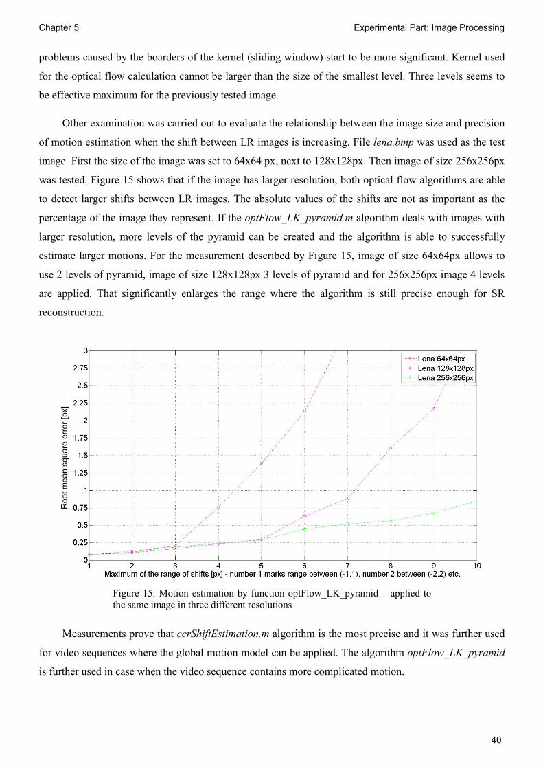
Other examination was carried out to evaluate the relationship between the image size and precision
of motion estimation when the shift between LR images is increasing. File lena.bmp was used as the test
image. First the size of the image was set to 64x64 px, next to 128x128px. Then image of size 256x256px
was tested. Figure 15 shows that if the image has larger resolution, both optical flow algorithms are able
to detect larger shifts between LR images. The absolute values of the shifts are not as important as the
percentage of the image they represent. If the optFlow_LK_pyramid.m algorithm deals with images with
larger resolution, more levels of the pyramid can be created and the algorithm is able to successfully
estimate larger motions. For the measurement described by Figure 15, image of size 64x64px allows to
use 2 levels of pyramid, image of size 128x128px 3 levels of pyramid and for 256x256px image 4 levels
are applied. That significantly enlarges the range where the algorithm is still precise enough for SR
reconstruction.
Measurements prove that ccrShiftEstimation.m algorithm is the most precise and it was further used
for video sequences where the global motion model can be applied. The algorithm optFlow_LK_pyramid
is further used in case when the video sequence contains more complicated motion.
Figure 15: Motion estimation by function optFlow_LK_pyramid – applied to the same image in three different resolutions
Root mean square error [px]
Chapter 6 Experimental Part: Video Processing
41
6 Experimental Part: Video Processing
In the previous chapter interpolation and motion estimation algorithms were examined using a set of
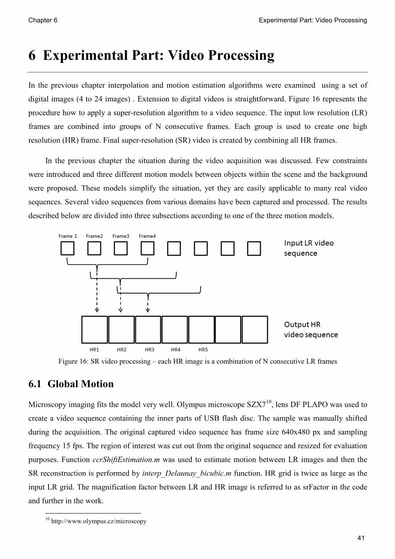
digital images (4 to 24 images) . Extension to digital videos is straightforward. Figure 16 represents the
procedure how to apply a super-resolution algorithm to a video sequence. The input low resolution (LR)
frames are combined into groups of N consecutive frames. Each group is used to create one high
resolution (HR) frame. Final super-resolution (SR) video is created by combining all HR frames.
In the previous chapter the situation during the video acquisition was discussed. Few constraints
were introduced and three different motion models between objects within the scene and the background
were proposed. These models simplify the situation, yet they are easily applicable to many real video
sequences. Several video sequences from various domains have been captured and processed. The results
described below are divided into three subsections according to one of the three motion models.
Figure 16: SR video processing – each HR image is a combination of N consecutive LR frames
6.1 Global Motion
Microscopy imaging fits the model very well. Olympus microscope SZX710, lens DF PLAPO was used to
create a video sequence containing the inner parts of USB flash disc. The sample was manually shifted
during the acquisition. The original captured video sequence has frame size 640x480 px and sampling
frequency 15 fps. The region of interest was cut out from the original sequence and resized for evaluation
purposes. Function ccrShiftEstimation.m was used to estimate motion between LR images and then the
SR reconstruction is performed by interp_Delaunay_bicubic.m function. HR grid is twice as large as the
input LR grid. The magnification factor between LR and HR image is referred to as srFactor in the code
and further in the work.
10 http://www.olympus.cz/microscopy
Chapter 6 Experimental Part: Video Processing
42
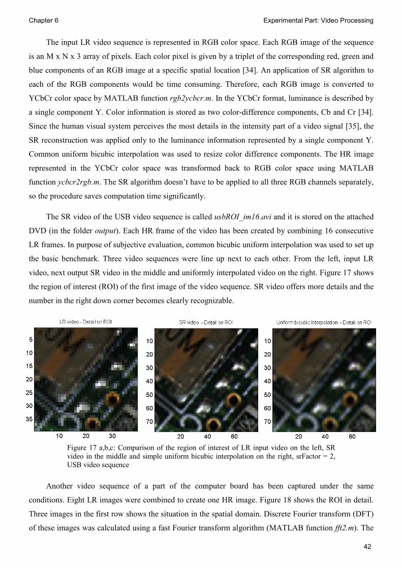
The input LR video sequence is represented in RGB color space. Each RGB image of the sequence
is an M x N x 3 array of pixels. Each color pixel is given by a triplet of the corresponding red, green and
blue components of an RGB image at a specific spatial location [34]. An application of SR algorithm to
each of the RGB components would be time consuming. Therefore, each RGB image is converted to
YCbCr color space by MATLAB function rgb2ycbcr.m. In the YCbCr format, luminance is described by
a single component Y. Color information is stored as two color-difference components, Cb and Cr [34].
Since the human visual system perceives the most details in the intensity part of a video signal [35], the
SR reconstruction was applied only to the luminance information represented by a single component Y.
Common uniform bicubic interpolation was used to resize color difference components. The HR image
represented in the YCbCr color space was transformed back to RGB color space using MATLAB
function ycbcr2rgb.m. The SR algorithm doesn’t have to be applied to all three RGB channels separately,
so the procedure saves computation time significantly.
The SR video of the USB video sequence is called usbROI_im16.avi and it is stored on the attached
DVD (in the folder output). Each HR frame of the video has been created by combining 16 consecutive
LR frames. In purpose of subjective evaluation, common bicubic uniform interpolation was used to set up
the basic benchmark. Three video sequences were line up next to each other. From the left, input LR
video, next output SR video in the middle and uniformly interpolated video on the right. Figure 17 shows
the region of interest (ROI) of the first image of the video sequence. SR video offers more details and the
number in the right down corner becomes clearly recognizable.
Figure 17 a,b,c: Comparison of the region of interest of LR input video on the left, SR video in the middle and simple uniform bicubic interpolation on the right, srFactor = 2, USB video sequence
Another video sequence of a part of the computer board has been captured under the same
conditions. Eight LR images were combined to create one HR image. Figure 18 shows the ROI in detail.
Three images in the first row shows the situation in the spatial domain. Discrete Fourier transform (DFT)
of these images was calculated using a fast Fourier transform algorithm (MATLAB function fft2.m). The
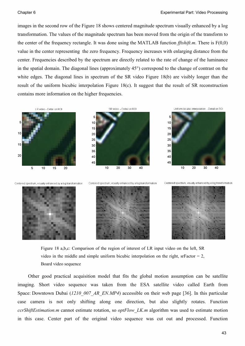
Chapter 6 Experimental Part: Video Processing
43
images in the second row of the Figure 18 shows centered magnitude spectrum visually enhanced by a log
transformation. The values of the magnitude spectrum has been moved from the origin of the transform to
the center of the frequency rectangle. It was done using the MATLAB function fftshift.m. There is F(0,0)
value in the center representing the zero frequency. Frequency increases with enlarging distance from the
center. Frequencies described by the spectrum are directly related to the rate of change of the luminance
in the spatial domain. The diagonal lines (approximately 45°) correspond to the change of contrast on the
white edges. The diagonal lines in spectrum of the SR video Figure 18(b) are visibly longer than the
result of the uniform bicubic interpolation Figure 18(c). It suggest that the result of SR reconstruction
contains more information on the higher frequencies.
Figure 18 a,b,c: Comparison of the region of interest of LR input video on the left, SR
video in the middle and simple uniform bicubic interpolation on the right, srFactor = 2,
Board video sequence
Other good practical acquisition model that fits the global motion assumption can be satellite
imaging. Short video sequence was taken from the ESA satellite video called Earth from
Space: Downtown Dubai (1210_007_AR_EN.MP4) accessible on their web page [36]. In this particular
case camera is not only shifting along one direction, but also slightly rotates. Function
ccrShiftEstimation.m cannot estimate rotation, so optFlow_LK.m algorithm was used to estimate motion
in this case. Center part of the original video sequence was cut out and processed. Function

Chapter 6 Experimental Part: Video Processing
44
interp_Delaunay_bicubic.m provides the SR reconstruction. Each HR image of the SR video is a
combination of 8 LR images. The SR video of the Dubai video sequence is called esa_dubai_full_im8.avi
and is stored on the attached DVD (in the folder output). Small region of interest from one image of the
sequence is shown in Figure 19.
6.2 Local Motion
Motion estimation (function optFlow_LK_pyramid.m) followed by SR reconstruction (function
interp_Delaunay_bicubic.m) was successfully applied to an artificial greyscale dataset called Otte's
Blockworld. The dataset was downloaded from the web site of Institute for Bio and Geosciences, Jülich,
Germany [37]. Each HR image of the SR video is a combination of 4 LR images. The resulting video can
be found on the attached DVD in folder Output, filename marble_LK_im4.avi.
Figure 19: Comparison of the region of interest of LR input video on the left, SR video in the middle and simple uniform bicubic interpolation on the right, srFactor = 2, Dubai video sequence
Figure 20: Frame 25 of the Corner video sequence, srFactor = 2, optFlow_LK_pyramid motion estimation, interp_Delaunay_bicubic interpolation

Chapter 6 Experimental Part: Video Processing
45
Good example satisfying the conditions of the local motion model is a car moving on the road
captured by a security camera. The situation was simulated by capturing a car video sequence by
Olympus digital camera XZ-1. Small ROI containing a car was cut out of the image sequence. To
estimate motion, optFlow_LK_pyramid.m algorithm was used. Function interp_Delaunay_bicubic.m
provides the SR reconstruction. Each HR image of the SR video is a combination of 4 LR images.
Figure 20 shows the 25th image of the sequence. Detail of the 25th frame is shown in Figure 21.
6.3 The Use of a Region of Interest
Video called lanciaRGB.avi captures a model of a car from the top view. Position of the camera
(Olympus XZ 1) is fixed. The aim is to obtain the sign on the roof in the best resolution possible. First the
region of interest is chosen manually. Then the program detects feature points using Harris detector
(function harris.m). On the next frame, surrounding of these feature points is searched and correlation
function is used to find new positions of the feature points (track_corr.m). A homography matrix (H) is
calculated from the knowledge of the positions of the feature points in two successive frames. The
homography matrix (H) can be formed from each quartet of points. Function ransac_h.m provides the
selection of an optimal matrix H that fits best the transformation between two successive frames.
Figure 22 a,b: Chosen region of interest is marked by the rectangle (on the left side). Feature points detected by Harris detector and their tracks during the first few frames (on the right side).
Figure 21: Comparison of the region of interest, srFactor = 2, Corner video sequence
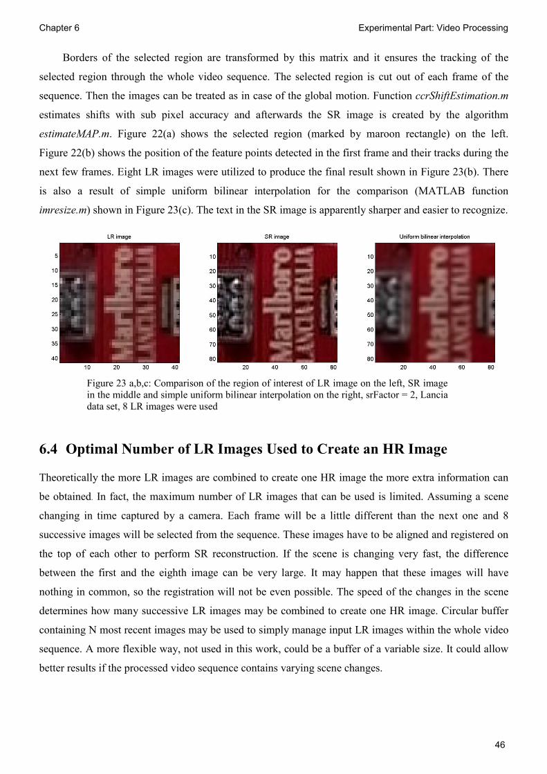
Chapter 6 Experimental Part: Video Processing
46
Borders of the selected region are transformed by this matrix and it ensures the tracking of the
selected region through the whole video sequence. The selected region is cut out of each frame of the
sequence. Then the images can be treated as in case of the global motion. Function ccrShiftEstimation.m
estimates shifts with sub pixel accuracy and afterwards the SR image is created by the algorithm
estimateMAP.m. Figure 22(a) shows the selected region (marked by maroon rectangle) on the left.
Figure 22(b) shows the position of the feature points detected in the first frame and their tracks during the
next few frames. Eight LR images were utilized to produce the final result shown in Figure 23(b). There
is also a result of simple uniform bilinear interpolation for the comparison (MATLAB function
imresize.m) shown in Figure 23(c). The text in the SR image is apparently sharper and easier to recognize.
6.4 Optimal Number of LR Images Used to Create an HR Image
Theoretically the more LR images are combined to create one HR image the more extra information can
be obtained. In fact, the maximum number of LR images that can be used is limited. Assuming a scene
changing in time captured by a camera. Each frame will be a little different than the next one and 8
successive images will be selected from the sequence. These images have to be aligned and registered on
the top of each other to perform SR reconstruction. If the scene is changing very fast, the difference
between the first and the eighth image can be very large. It may happen that these images will have
nothing in common, so the registration will not be even possible. The speed of the changes in the scene
determines how many successive LR images may be combined to create one HR image. Circular buffer
containing N most recent images may be used to simply manage input LR images within the whole video
sequence. A more flexible way, not used in this work, could be a buffer of a variable size. It could allow
better results if the processed video sequence contains varying scene changes.
Figure 23 a,b,c: Comparison of the region of interest of LR image on the left, SR image in the middle and simple uniform bilinear interpolation on the right, srFactor = 2, Lancia data set, 8 LR images were used
Chapter 7 Discussion
47
7 Discussion
7.1 Comparison of SR Approaches
Several different SR methods were studied. The frequency approach is simple in theory and these
algorithms are also fast for computational efficiency. However, the observation model is limited by the
principle of the method to the global translational motion. Moreover in the frequency domain, it is often
difficult to express the prior knowledge that could be used to constrain the SR problem. Therefore, the
work was focused on non-uniform and statistical methods.
Nine non-uniform interpolation methods were implemented in MATLAB, their PSNR, MSSIM and
processing times measured. Non-uniform methods are computationally efficient (especially shift and add
algorithms). Delaunay bicubic interpolation provided the best tradeoff between speed and image quality
performance. The major advantage of the non-uniform approach is the relatively small computational
load which makes real-time applications possible. However, the restoration part does not consider errors
that are generated during the interpolation process. Therefore, optimality of the estimation is not
guaranteed. Additionally, the reconstruction process does not take directly into account blurring and noise
of input LR images. Noise can be minimized in the pre-processing step and deblurring can follow after
the reconstruction in so called restoration step.
Statistical approaches model the process of creation of LR images and then prior terms are used to
regularize the ill-posed nature of the SR inverse problem. MAP estimation method with gradient descent
minimization was programmed. More precise description of the observation problem allows to
reconstruct the HR images with better visual quality and more details at high spatial frequencies then
non-uniform methods. This stochastic SR approach using Bayesian framework provides robustness and
flexibility in modeling noise characteristics and a prior knowledge can be easily used to regularize the SR
inverse problem. Thus, Bayesian treatments are promising for SR reconstruction. However, model
parameters have to take simple parametric forms because of the high computational demand of these
algorithms. Large simplification of observation models and computational demands could restrict the
usage of these methods for dealing with more complex cases that may happen in real applications.
To apply SR to real video sequences, precise motion estimation is necessary. The registration errors
are crucial for further image processing. Relative motion between the camera and the scene can be in
general very complex. That makes sub pixel precise motion estimation the very challenging task. If some
constraints are introduced, difficult complex model is simplified, yet it remains suitable description for
many real video sequences.

Chapter 7 Discussion
48
Tested video sequences were divided according to their motion model into three different cases.
First case supports the global motion model, second case contains local motions. In the third case, region
of interest is tracked through the sequence, cropped and then it may be treated as the global motion case.
The last approach works even if the video includes more complex relative motion as long as the
transformation model between two successive frames can be described by homography matrix. Five
motion estimation algorithms based on 3 different principles were programmed and evaluated with
respect to precision and computational load. Algorithm based on normalized cross correlation function
(ccrShiftEstimation.m) has the best performance for global motion model. In case of different local
motions, algorithm called optFlow_LK_pyramid.m has achieved the best results.
7.2 Real Video Applications
The most suitable SR methods mentioned above were successfully applied on real video sequences from
different domains. Global motion model is suitable for video sequences obtained by microscopy imaging.
Olympus microscope SZX7, lens DF PLAPO was used to create a video sequence showing the inner parts
of USB flash disc. Motion estimation using normalized cross correlation function and Deunay bicubic
reconstruction were successfully applied. Final SR video sequence is up sampled twice and stored on the
attached DVD (usbROI_im16.avi).
Satellite imaging could also fits well for the global motion model. Tested video sequence Earth from
Space: Downtown Dubai11 contains only shifting along one direction, but also slightly rotates. Therefore
LK optical flow algorithm was suitable for motion estimation. SR video is stored on the attached DVD as
esa_dubai_full_im8.avi.
Good example satisfying the conditions of the local motion model is a car moving on the road
captured by a security camera. The situation was simulated by capturing a car video sequence by a
common digital camera. SR video was successfully created by Delaunay interpolation and it is also part
of the attached DVD (file cornerROI_LK.avi). Motion estimation based on the optical flow provides very
good results if the video meets the preliminary assumptions about the smoothness of motion and constant
pixel values along the motion trajectories. Difficulties occur if these assumptions fail.
Quick movements cause large changes of the scene between successive frames. If the object changes
the position between the successive frames for more than approximately 5 % of the picture size in the
direction of motion, then the precision of implemented optical flow algorithm decline significantly. Very
large interframe displacements complicate the possibility to obtain information about the moving object
from the adjacent frames. Other issues are caused by occlusions of the moving objects, changes of their
11 ESA satellite video (1210_007_AR_EN.MP4) - multimedia.esa.int

Chapter 7 Discussion
49
shapes (not rigid objects) or by variations in illumination. Motion blur is another important problem and
considering of it would significantly increase computational complexity.
SR reconstruction allows overcoming the limits of the optical systems and improves the
performance of the image processing applications. SR is fully based on digital signal processing
techniques, so no hardware changes are necessary. It could be particularly useful in microscopy, thermal
imaging and medical applications. SR was applied in low radiation digital X-ray mammography and in
optical coherence tomography with great results [47]. Any new information recovered from video
evidence can potentially be very valuable in the forensic field. In this case, investigators are often
concerned only in a small region of interest. ROI can be tracked through the video sequence, cropped and
obtained information is used for SR reconstruction. This procedure was tested with the video
lanciaRGB.avi. MAP estimation method provide very promising results.
7.3 Advanced Issues
The key to successful SR conversion of the SDTV video signal to the HDTV lies in a robust and effective
motion estimation. Videos generally contains very complex relative motions. Precise motion estimation is
very challenging task referring to many problems mentioned above.
Computational complexity limits wider real SR applications. SR algorithms need to be reasonably
fast if they should be practical for use to a large number of users. The non-uniform interpolation approach
seems to be suitable for real time applications since it has relatively low computational cost. However,
stochastic approach, namely MAP estimation, is able to regularize better the SR inverse problem. The
observation model is more precise and it leads to greater enhancement of the resulting HR images. The
disadvantage of this method is the higher computational cost. Therefore, the algorithm extensions should
be provided to increase the computational speed.
In practical situations, the blurring process is often unknown. It is convenient to incorporate the blur
identification process into the SR reconstruction. Šroubek, Flusser and Cristóbal proposed a method that
simultaneously estimates the HR image and the blur kernel [49]. They achieved impressing results, but
their motion model is only translational. Ce Liu and Dequing Sun went further in super-resolving real-
world sequences. They proposed a Bayesian approach that simultaneously estimates underlying motion,
blur kernel and noise level while reconstruction the original HR images [44]. The results suggest that their
algorithm is actually probably the best in class, yet the computation load is huge and the algorithm has
problems if scenes do not meet the graphical model assumptions.12 The authors state that “C++
implementation takes about two hours on an Intel Core i7 Q820 workstation with 16 GB RAM when
super resolving a 720 x 480 frame using 30 adjacent frames at an up-sampling factor of 4.”[44]. 12 http://research.microsoft.com/en-us/um/people/celiu/cvpr2011/

Chapter 7 Discussion
50
The effects of video compression on SR performance should be also investigated since real common
user videos are usually compressed. The observation model could be further extended by an additional
component which would consider the errors caused by the compression of the observed LR images.
A challenging SR problem is the lack of a suitable objective metric for assessment of the quality of
the image created by SR reconstruction. PSNR and MSSIM are widely used among image processing
experts. It can be used for SR in a prepared experiment with the synthetic data set. However, the reference
image is not known in the real scenarios. MSE error based measurements are not able to describe how
much the image has improved visually. Therefore, Šroubek et al. did not even use in their work [48] any
measure of reconstruction quality and left the printed results to a human eye comparison only.
Chapter 8 Conclusions
51
8 Conclusions
The first part of the thesis presents a survey of SR methods for digital image and video processing.
Various SR approaches and their exact mathematical description were extensively studied.
For purpose of this work, eight SR reconstruction algorithms and five algorithms for motion
estimation were programmed in MATLAB elaborated with respect on published articles. Subjective
image quality, PSNR, MSSIM, processing time and accuracy of implemented algorithms have been tested
on still images and videos.
An optimal SR method applicable to real video sequences should be reasonably quick, able to
process a large number of color images and achieve very good image quality of the output under different
circumstances. Attention was focused mainly on the non-uniform interpolation SR approach, because of
its lower computational demand.
Delaunay bicubic non-uniform interpolation has proved as the best method fulfilling maximum
desired requirements for image quality, computational speed and versatility with respect to different
motion models, number of LR images used and up sampling factor. MAP estimation algorithm with
gradient descent minimization reconstructs the HR images with better visual quality then non-uniform
methods, but it is approximately 8 times slower than Delaunay bicubic non-uniform interpolation.
Motion estimation can be very challenging task. If it is not precise, the overall super-resolution
method is unsuccessful. In this work, 3 different motion models were assumed: global motion, different
local motions and the use of a region of interest only. The normalized cross correlation algorithm has
been proved to be the most suitable in the first and third case. Lucas-Kanade optical flow using pyramidal
approach has provided the best results in case of local motion.
The most suitable algorithms have been successfully applied on real video sequences from different
domains such as microscopy imaging, satellite imaging, common consumer videos. Resulting SR video
sequences provide image quality superior to standard uniform interpolation techniques.
Bayesian approach using MAP estimation is promising, but computational complexity could limit
wider real SR applications. Therefore the algorithm extensions should be provided to increase the
computational speed. The effects of video compression on SR performance should be also investigated
since common videos are usually compressed. Optimization of visual impact with respect to the time
spent on the image processing could be another research task. Very promising is the application of SR in
medical and biological imaging as well as for purposes of forensic science.
References
52
References
[1] MILANFAR, Peyman. Super-resolution Imaging, CRC Press, 2011. 472s.
[2] CHAUDHURI, Subhasis. Super-resolution Imaging. Kluver Academic Publishers, New York, 2002. 279s.
[3] FOROOSH, Hassan; ZERUBIA Josiane; BERTHOLD, Marc, Extension of Phase Correlation to Subpixel
Registration, IEEE Transactions on Image Processing, Vol. 11, NO.3,March 2002
[4] VANDEWALLE, Patrick, Super-resolution from unregistered aliased images, ÉCOLE POLYTECHNIQUE
FÉDERALE DE LAUSANNE, Disertační práce, 2006. 129s.
[5] KOC, U.; LIU, K., Interpolation-free subpixel motion estimation techniques in dct domain. IEEE Trans. Circuits
Syst. Video Technol., vol. 8 pp. 460-487, Aug. 1998.
[6] HORN, Berthold; SCHUNCK Brian. Determining Optical Flow. Massachusetts Institute of Technology Artificial
Intelligence Laboratory. Memo NO. 572, April 1980
[7] International Organization for Standardization, "ISO 12233:2000 - Photography - Electronic still picture cameras -
Resolution measurements," 2000.
[8] PARK, Sung Cheol; PARK Min Kyu; KANG, Moon Gi, Super-Resolution Image Reconstruction: A Technical
Overview, IEEE Signal Processing Magazine, pp. 21-36, May 2003.
[9] KOMATSU, T.; AIZAWA, K.; IGARASHI, T. and SAITO, T., Signal-processing based method for acquiring very
high resolution image with multiple cameras and its theoretical analysis, Proc. Inst. Elec. Eng., vol. 140, no. 1, pp.19-
25, Feb. 1993
[10] Testo company [online]. 2012 [cit. 2012-06-03]. Dostupný z www:
<http://www.testosites.de/thermalimaging/en_INT/index.html?tb=11_superresolution#/0/19/>
[11] KATSAGGELOS, Aggelos; MOLINA, Rafael; MATEOS, Javier, Super Resolution of Images And Video, Morgan
& Claypool Publishers, 2007.
[12] BOUŠE, J.; LUKEŠ, T.; ŠEBEK, J., Semestrální projekt: Super-resolution, ČVUT v Praze, 2012. 15s.
[13] WYAWAHARE, M.V.; PATIL, P.M.; ABHYANKAR H.K., Image Registration Techniques: An overview,
International Journal of Signal Processing, Image Processing and Pattern Recognition, Vol. 2, No. 3, September 2009.
[14] ZITOVÁ, B.; FLUSSER, J., Image registration methods: a survey, Image and Vision Computing, vol. 21, no. 11,
pp. 997-1000, 2003.
[15] CAPEL, D.; ZISSERMAN, A., Computer vision applied to super-resolution, IEEE Signal Processing Magazine,
vol. 20, no. 3, pp. 75-86, May 2003.

References
53
[16] CHAN, Stanley, H., VO, D., T.; NGUYEN T., Q., Subpixel motion estimation without interpolation, ECE Dept,
UCSD, La Jolla, CA 92092-0407, August 2010.
[17] BORMAN, S; ROBERTSON, M., A; STEVENSON, R. L., Block-matching sub-pixel motion estiamtion from noisy
under-sampled frames - An empirical performance evaluation, University of Notre Dame, Nontre Dame, IN 46556,
USA, July 1998.
[18] ALAM, M.,S., BOGNAR, J.G., HARDIE R.,C.; YASUDA, B.,J., Infrared Image Registration and Hight-resolution
Using Multiple Translationally Shifted Aliased Video Frames, IEEE Transactions on Instrumentation and Measurement,
vol. 49, no. 5, October 2000
[19] BAKER, Simon, MATTHEWS, Iain, Lucas-Kanade 20 Years On: A Unifying Framework, International Journal of
Computer Vision, vol. 56(3), pp. 221-255, 2004.
[20] DEBELLA-GILO, M.; Kääb A.; Subpixel precision image matching for displacement measurement of mass
movements using normalized cross-correlation, ISPRS TC VII Symposium, vol. 38, part 7B, Vienna, Austria, July,
2010.
[21]TIAN, Q.; HUHNS, M., N., Algorithms for Subpixel Registration, Computer Vision, Graphics, and Image
Processing, vol. 35, pp. 220-233, 1986.
[22] REDD, R., A., Comparison of Subpixel Phase Correlation Methods for Image Registration, Arnold Enginnering
Development Center Arnold Air Force Base, Tennessee, USA, April, 2010.
[23] GUIZAR-SICAIROS, M; THURMAN, Samuel, T., and FIENUP, James, R., Efficient Subpixel Image Registration
Algorithms, Optics Letters, vol. 33, no. 2, pp. 156-158, January, 2008.
[24] LERTRATTANAPANICH, S.; BOSE, N., K., High resolution image formation from low resolution frames using
Delaunay triangulation, IEEE Transactions on Image Processing, vol. 11, pp. 1427 - 1441, December 2002.
[25] GILMAN, A.; BAILEY, D., G., Near optimal non-uniform interpolation for image super-resolution from multiple
images, Institute of Information Sciences and Technology, Massey University, Palmerston North, 2006.
[26] TSAI, R., Y.; HUANG, T., S., Multipleframe image restoration and registration, Advances in Computer Vision
and Image Processing, Greenwitch, CT: JAI Press Inc., pp. 317 - 339, 1984.
[27] HONG, M.,C.; KANG, M., G.; KATSAGGELOS, A., K., A regularized multichannel restoration approach for
globally optimal high resolution video sequence, SPIE VCIP, vol. 3024, pp. 1306-1317, San JOse, CA, February 1997
[28] SHULTZ, R., STEVENSON, R., Extraction of high-resolution frames from video sequences. IP5, pp. 996-1011,
June 1996.
[29] STILLER, CHRISTOPH; KONRAD, JANUSZ, Estimating Motion in Image Sequences, IEEE Signal Processing
Magazine, pp. 36, July 1999.
[30] IRANI, M.; PELEG, S., Improving resolution by image registration. CVGIP: Graph Models Image Process, vol. 53,
pp. 231-239, 1991.
References
54
[31] BOSE, N.K.; KIM, H., C.; VALENZUELA, H., M., Recursive implementation of total least squares algorithm for
image reconstruction from noisy, undersampled multiframes, IEEE Conf. Acoustics, Speech and Signal Processing,
Minneapolis, vol. 5, pp. 269-272, April 1993
[32] RHEE, S., H.; KANG, M., G., Discrete cosine transform based regularized high-resolution image reconstruction
algorithm, Opt. Eng. vol. 38, no. 8, pp. 1348-1356, August 1999
[33] MARQUES, O., Practical image and video processing using MATLAB, Wiley, 2011. 639s.
[34] GONZALEZ, C.,RAFAEL; WOODS, E., RICHARD; EDDINGS, L., STEVEN, Digital image processing using
MATLAB, Gatesmark Publishing; 2nd edition, 2009. 827s.
[35] BURGER, WILHELM; BURGE, J.,MARK, Principles of Digital Image Processing, Springer, 2009. 260s.
[36] ESA online videos [online]. 2012 [cit. 2012-12-09]. Dostupný z www: < http://multimedia.esa.int/ >
[37] Institute for Bio and Geosciences [online]. 2012 [cit. 2012-12-12]. Dostupný z www:
< http://www2.fz-juelich.de/icg/icg-3/Mitarbeiter/Scharr/Testdata >
[38] University of Waterloo [online]. 2012 [cit. 2012-12-13].Dostupný z www:
< https://ece.uwaterloo.ca/~z70wang/research/ssim/ >
[39] WANG, ZHOU; BOVIK, ALAN C.; SHEIKH, HAMID R.; SIMONCELLI, EERO P., Image Quality Assessment:
From Error Visibility to Structural Similarity, IEEE Transactions on Image Processing, vol. 13, no. 4, April 2004
[40] HORN, K.,P., BERNOLD; SCHUNCK, BRIAN, G., Determining Optical Flow, Massachusetts Institute of
Technology, Artificial Intelligence Laboratory, A.I. Memo No. 572, April 1980
[41] LUCAS, B.,D.; KANADE, T., An Iterative Image Registration Technique with an Application to Stereo Vision,
Proceedings of Imaging Understanding Workshop, pp. 121-130, 1981
[42] DAVIES, E.R., Computer and machine vision, Theory, algorithms, practicalities, Elsevier, Oxford, 2012. 871s.
[43] FENG-QUING, QIN, Blind Video Super Resolution Reconstruction Based on Error-Parameter Analysis Method,
2nd International Conference on Industrial Mechatronics and Automation, 2012.
[44] LIU,C.; SUN, D., A Bayesian Approach to Adaptive Video Super Resolution, IEEE Conference on Computer Vision
and Pattern Recognition (CVPR), pp. 209 -216, 2011
[45] A Bayesian Approach to Adaptive Video Super Resolution [online]. 2011 [cit. 2012-12-17]. Dostupný z www:
< http://research.microsoft.com/en-us/um/people/celiu/cvpr2011/ >
[46]MUDUGAMUWA, D.J.; HE, X. JIA, W., Efficient Super-Resolution by Finer Sub-Pixel Motion Prediction and
Bilateral Filtering, IEEE International Conference on Multimedia and Expo, pp.800-805, 2012

References
55
[47] ROBINSON M.D; CHIU S.J.; LO J.Y.; TOTH C.A.; IZATT J.A; FARSIU S, "Novel Applications of Super-
Resolution in Medical Imaging", Book Chapter in Super-Resolution Imaging, Peyman Milanfar (Editor), CRC Press,
pages 383-412, 2010
[48] ŠROUBEK F.; FLUSSER J.; CRISTOBAL G., Super-Resolution and Blind Deconvolution For Rational Factors
With an Application to Color Images , Computer Journal vol.52, 1 (2009), p.
142-152
[49] ŠROUBEK F., CRISTOBAL G., FLUSSER J., Simultaneous super-resolution and blind deconvolution, Journal of
Physics: Conference Series vol.124, p. 1-8, 4th AIP International Conference and the 1st Congress of the IPIA,
(Vancouver, CA, 25.06.2007-29.06.2007)
[50] HELLEU, LOIC, Advanced Image Reconstruction Algorithms, Super-Resolution, Diploma Thesis, CTU in Prague,
2009. 50s.
Appendix
56
Appendix: Contend of the attached DVD
TomasLukes_DiplomaThesis_Super-Resolution_Methods.pdf
ReadMe.txt
[output]
usbROI_im16.avi
usbComparison_zoom_im8_sr2.tif
RGBLenaComparison_all.tif
RGBLena_Comparison_im8_sr2.tif
marble_LK_im4.avi
MAP_tracking_im8_sr4_iter30.tif
export_trackPts.avi
export_lanciaRGB.avi.avi
esa_dubai_full_im8.avi
cornerROI_zoom.tif
cornerROI_LK.avi
cornerROI_25th_frame.tif
boardComparison_zoom_im8_sr2.tif
bfly_MAP_im16_sr4_iter30.tif
[SR of images]
testing_PSNR_MSSIM.m
testing_MAP.m
showRGBLenaImages_sr2.m
showPROBLEMofObjectiveEvaluation.m
showGreyLenaImages_sr2.m
show_PSNR_MSSIM.m
[SR of images\dataset]
lenaROI.bmp
lenaRGB.bmp
lena512.bmp
createDatasetRGB2.m
createDatasetRGB1.m
createDataset2.m
createDataset1.m
cameramanROI.tif
bfly.jpg
[SR of images\interpolation]
nearestNeighbour1.m
nearestNeighbour_shiftAdd2.m
nearestNeighbour_shiftAdd1.m
nearestNeighbour_fast.m
iterativeBackProjection.m
interp_nearOptimal.m
interp_Delaunay_bicubic.m
interp_Delaunay.m
interp_bilinear_fast.m
costFunc.m
[SR of images\MAP_approach]
TransMat.m
sptoeplitz.m
LinearKernel.m
estimateMAP.m
DecMat.m
costFunction.m
[SR of images\measuredData]
vysledkyTestPSNR_MSSIM_15112010.mat
[SR of images\metrics]
ssim_index.m
[SR of images\registration]
optFlow_LK_pyramid.m
optFlow_LK.m
ccrShiftEstimation_fast.m
ccrShiftEstimation.m
blockMatching.m

Appendix
57
[SR of videos]
videoSR2.m
videoSR1.m
trackingSR.m
testing_MotionEstimation.m
showTestingME2.m
showTestingME.m
prepareVideo.m
plotFlow.m
[SR of videos\dataset]
lenaROI.bmp
lena512.bmp
createDataset2.m
[SR of videos\dataset\microscope_videos]
usbROI.avi
usb.avi
board3ROI.avi
board3.avi
[SR of videos\dataset\videos]
lanciaRGB.avi
esa_dubaiROIa.avi
cornerROI.avi
[SR of videos\interpolation]
nearestNeighbour_shiftAdd2.m
nearestNeighbour_shiftAdd1.m
iterativeBackProjection.m
interp_Delaunay_bicubic.m
interp_Delaunay.m
[SR of videos\MAP_approach]
TransMat.m
sptoeplitz.m
LinearKernel.m
estimateMAP.m
DecMat.m
costFunction.m
[SR of videos\export]
supResData.mat
[SR of videos\measuredData]
testing_MotionEstimationL50_64px.mat
testing_MotionEstimationL50_256px_4N.mat
testing_MotionEstimationL50_128px.mat
testing_MotionEstimationC50.mat
[SR of videos\registration]
optFlow_LK_pyramid.m
optFlow_LK.m
ccrShiftEstimation_fast.m
ccrShiftEstimation.m
blockMatching.m
[SR of videos\trackingRGB]
u2h.m
track_init.m
track_corr.m
sample.m
ransac_h.m
processMpvVideo.m
processMpvInit.m
processMpvFrame.m
nsamples.m
nonmaxsup2d.m
hdist.m
harris_response.m
harris.m
getPatchSubpixel.m
getLimits.m
gaussfilter.m
gaussderiv.m
gausscutoff.m
gauss.m
filter_boundaries.m
corr2u.m