Faculty of Science, Engineering and Sustainability

School of Engineering and Energy

A report submitted to the School of Engineering and Energy,

Murdoch University in partial fulfilment of the requirements for the

degree of Bachelor of Engineering

Super-capacitor/Lead Acid Battery Hybrid Energy

Storage Suitable for Remote Area Power Supply

(RAPS) Systems.

Bruce Blechynden 30657983

19th November 2010

i

Academic Supervisor endorsement

I am satisfied with the progress of this thesis project and that the attached report is an

accurate reflection of the work undertaken.

Signed

Date

iii

Abstract

This paper presents the results of simulations based on real load data collected from a

RAPS system in the south west of Western Australia. The load data was collected at a

rate of one sample per second to capture the transient changes. The data had features of

a base load suited to lead-acid batteries and transient spikes in load suited to super-

capacitors.

A model of a RAPS energy storage system including batteries and super-capacitors was

built in Simulink. This model was designed to capture the major influences on battery

life and performance: battery current, state of charge and battery temperature.

Simulations were run under standard conditions of no diesel generation (solar

generation only), fixed ambient temperature (25°C), fixed total energy storage of 875Ah

and equal hours of daylight and darkness.

An optimum super-capacitor size of 65Ah capacity was identified for the conditions of

the simulation.

Battery temperature was found to be dominated by ambient temperature and little

improvement was achieved by including super-capacitors.

Battery life was improved by seven months from nine years and fourteen weeks to nine

years and forty one weeks.

With the use of a 65Ah super-capacitor equivalent performance to the battery only base

case can be achieved with a battery of 460Ah, approximately half the capacity of the

existing batteries.

A 450Ah battery bank costs by $3520 less than the 875Ah battery bank used in the

RAPS system that was monitored. A 65Ah super-capacitor costs between $115 500 and

$147 500 indicating that a reduction in price in the order of forty times is necessary

before super-capacitors could be justified in a battery super-capacitor hybrid energy

store.

iv

Acknowledgments

My sincere thanks go first of all to my wife Bernadine for her support, encouragement

and understanding, not only during the period of this thesis but also the four years of

study leading up to this point. Likewise our children Eligh Asher and Tabitha who now

consider the odd hours and habits of a student common place and no doubt expect the

relative freedoms of student lifestyle to continue when the pressures of career and

mortgage commence shortly.

This project would not have taken the shape it has without the assistance of Dan and

Jody Wildy who kindly allowed me access to their home and RAPS system, going so

far as to catalogue their appliance use so I could match data to device. Unfortunately

Dan, it appears super-capacitors are out of reach for the time being, but then it wasn’t so

long ago that solar panels were a dream as well.

Thanks also to Murdoch’s RISE institute for access to their power quality meter used to

monitor Dan and Jody’s RAPS system.

Finally to the staff of Murdoch University School of Engineering and Energy, without

whose hard work and assistance I would not have reached this point: particularly Dr

Gareth Lee who supervised this project, providing direction and insight where needed to

guide it to completion.

v

Table of Contents Academic Supervisor endorsement .................................................................................... i

Abstract ............................................................................................................................ iii

Acknowledgments ............................................................................................................ iv

Table of Contents .............................................................................................................. v

List of Figures & Tables ................................................................................................. vii

1. Introduction ............................................................................................................... 1

2. RAPS Systems .......................................................................................................... 2

3. Lead Acid Batteries ................................................................................................... 3

3.1 Background ....................................................................................................... 3 3.2 Operation ........................................................................................................... 3 3.3 Gassing .............................................................................................................. 5 3.4 Capacity: the Peukert Effect ............................................................................. 5 3.5 Internal Resistance ............................................................................................ 7 3.6 Battery Life ....................................................................................................... 9 3.7 Efficiency ........................................................................................................ 11 3.8 Temperature Effects ........................................................................................ 11 3.9 Battery Charging ............................................................................................. 13 3.10 Battery Charging with Photo Voltaics ............................................................ 18

4. Super - capacitors .................................................................................................... 20

4.1 Background ..................................................................................................... 20 4.2 Operation ......................................................................................................... 21 4.3 Capacity........................................................................................................... 23 4.4 DC/DC Converters .......................................................................................... 24 4.5 Fundamentals .................................................................................................. 25 4.6 Internal Resistance .......................................................................................... 26 4.7 Capacitor Life.................................................................................................. 28 4.8 Temperature Effects ........................................................................................ 29

5. Strengths of Lead Acid Batteries and Super-capacitors .......................................... 30

6. Data Collection........................................................................................................ 31

6.1 The RAPS System ........................................................................................... 31 6.2 The Data Taker ................................................................................................ 38 6.3 The Data .......................................................................................................... 38

7. Matching Super-capacitors to Load ........................................................................ 39

7.1 Super-capacitor Sizing .................................................................................... 40 8. RAPS System Model .............................................................................................. 45

8.1 State of Charge (SOC) .................................................................................... 45 8.2 Internal Resistance .......................................................................................... 47 8.3 Heat Generation and Battery Temperature ..................................................... 48 8.4 Load and Battery Current ................................................................................ 53 8.5 The Capacitor .................................................................................................. 55 8.6 Modelling Issues ............................................................................................. 57

9. Simulation Results .................................................................................................. 58

vi

10. Discussion ............................................................................................................... 71

10.1 The Problem .................................................................................................... 71 10.2 The Investigation ............................................................................................. 71 10.3 The Solution .................................................................................................... 75

11. Conclusion .............................................................................................................. 80

12. Future Work ............................................................................................................ 82

13. References ............................................................................................................... 83

14. Appendix ................................................................................................................. 86

vii

List of Figures & Tables Figure 1 Lead-acid Battery................................................................................................ 4

Figure 2 Battery Capacity (Peukert) Curve ....................................................................... 6

Figure 3 Simple Battery Model ......................................................................................... 7

Figure 4 Battery Discharge Voltage Curve ....................................................................... 9

Figure 5 Battery Life/DOD Curve Showing Trend-line for Battery Life Calculations .. 10

Figure 6 Battery Life/Temperature Curve....................................................................... 12

Figure 7 Single Step Constant Current Charging ............................................................ 13

Figure 8 Two Step Constant Current Charging .............................................................. 14

Figure 9 Constant Voltage Charging .............................................................................. 15

Figure 10 Taper Current Charging .................................................................................. 16

Figure 11 Constant Current Constant Voltage Charging ................................................ 17

Figure 12 Solar Panel IV Curve ...................................................................................... 18

Figure 13 Conventional Capacitor .................................................................................. 21

Figure 14 EDLC (Super-capacitor) ................................................................................. 23

Figure 15 DC/DC Converter [12]. .................................................................................. 24

Figure 16 Capacitors Connected (a) in Parallel and (b) in Series. .................................. 25

Figure 17 Simple Capacitor Model ................................................................................. 26

Figure 18 Capacitor Voltage Profile at Constant Current Discharge [13] ...................... 27

Figure 19 Capacitance Decrease while Cycling at Different Voltages [14] ................... 28

Figure 20 Capacitance and Internal Resistance Variation with Temperature [14] ......... 29

Figure 21 Ragone Plot of Energy Storage Devices [17] ................................................. 30

Figure 22 2.4kW Solar Array .......................................................................................... 32

Figure 23 48 Volt Battery Bank ...................................................................................... 33

Figure 24 11kVA Generator............................................................................................ 34

Figure 25 Switchboard Containing Metering and MPPT ............................................... 35

Figure 26 Inverter and System Controller ....................................................................... 36

Figure 27 Data Collection ............................................................................................... 37

Figure 28 Load Profile 04 September 2010. ................................................................... 38

Figure 29 Daily Load and Daily Solar Production.......................................................... 39

Figure 30 Simulink Battery Model ................................................................................. 47

Figure 31 Simulink Heat Generation Model ................................................................... 49

Figure 32 Simulink Battery Temperature Model ............................................................ 52

Figure 33 Simulink Load and Generation Model ........................................................... 54

viii

Figure 34 Simulink Capacitor Model .............................................................................. 56

Figure 35 Base Case Battery Only: Net Battery Current ................................................ 59

Figure 36 Optimum Case with 65Ah Capacitor: Net Battery Current ............................ 60

Figure 37 Optimum Case with 65Ah Capacitor: Net Capacitor Current ........................ 61

Figure 38 Base Case Battery Only: Battery SOC ........................................................... 62

Figure 39 Optimum Case with 65Ah Capacitor: Battery SOC ....................................... 63

Figure 40 Base Case Battery Only: Battery Temperature ............................................... 64

Figure 41 Optimum Case with 65Ah Capacitor: Battery Temperature .......................... 65

Figure 42 Battery Efficiency ........................................................................................... 66

Figure 43 Battery Average SOC ..................................................................................... 66

Figure 44 Average Battery Current ................................................................................. 67

Figure 45 System Efficiency ........................................................................................... 67

Figure 46 Average PV Current ....................................................................................... 68

Figure 47 Average Temperature ..................................................................................... 69

Figure 48 Maximum Temperature .................................................................................. 69

Figure 49 Spring Case: Fixed Super-capacitor Variable Battery .................................... 70

1

1. Introduction Super-capacitors are efficient energy storage devices that have been developed in recent

years into products that can be used in electrical power applications for energy storage.

Renewable energy systems by their intermittent nature are dependent on energy storage

and/or traditional fossil fuel generation to maintain reliable electricity supply.

Remote Area Power Supply (RAPS) systems incorporating renewable energy often

utilise both traditional generation and energy storage, usually in the form of lead acid

batteries. Batteries represent a significant cost, both initially and during the lifetime of

the system, as they will require replacing several times.

Super-capacitors are suited to supplying loads of short duration and high power, while

batteries are better suited to supplying loads of long duration and low power. The loads

on a domestic RAPS system are a combination of long duration low power demand and

short duration high power spikes in demand.

The relative strengths of batteries and super-capacitors lend themselves to supplying the

two components of RAPS load. This project seeks to quantify what gains may be made

by combining lead acid batteries and super-capacitors in a hybrid energy storage system

and dispatching the two components to supply the load components suited to their

strengths.

2

2. RAPS Systems Remote Area Power Supply (RAPS) systems as the name suggests are stand alone

power systems isolated from the grid and typically found in remote areas. They are also

a viable alternative to grid connection in rural areas due to high cost or difficulty of

connecting to the grid, government subsidies for renewable energy generation and

people’s desire to embrace cleaner alternatives to conventional electricity generation.

RAPS systems need not include renewable generation however the obvious benefits of

reducing dependence on fossil fuels and the increased availability and affordability of

renewable, (particularly solar) generation for domestic users makes solar generation

combined with battery energy storage and diesel backup an attractive and financially

viable RAPS option.

3

3. Lead Acid Batteries

3.1 Background

The first battery consisting of alternating discs of zinc and copper separated by cloth

soaked in salty water was documented in 1800 by Alessandro Volta [1]. In 1859 the

lead acid battery was introduced by Gaston Plante [1] and remains one of the most

common batteries available today.

There are two broad groups of lead acid batteries: flooded cell batteries are the

conventional battery containing liquid electrolyte and are vented to the atmosphere.

Valve Regulated Lead Acid (VRLA) batteries contain an electrolyte paste (gel) [2] or

absorbent glass mat (AGM) [2] and are supposedly maintenance free or low

maintenance. They are not vented to atmosphere unless there is excessive pressure build

up.

Lead acid batteries also vary according to their application. Car batteries are designed

for high current over a short duration. Deep cycle batteries are designed to discharge

slowly over long periods. They may be flooded or VRLA type and their internal

construction will vary accordingly.

3.2 Operation

A lead acid battery consists of alternating plates of lead (Pb) and lead oxide (PbO2)

immersed in an electrolyte of sulphuric acid (H2SO4). Modern batteries use an injection

moulded casing of polypropylene [3] or similar to contain the plates and electrolyte.

Often a synthetic polymer or glass matt separator is used [3] between the plates to keep

them from touching as illustrated in Figure 1.

4

Figure 1 Lead-acid Battery

The chemical half equations are shown below. When a conductor is connected between

the anode and cathode electrons flow, the battery discharges and the chemical reaction

occurs. At the anode oxidation takes place. The reaction is given by:

Pb + HSO4¯ → PbSO4 + H+ + 2e¯ (+1.69 volts) Equation 1

At the cathode reduction takes place. The cathode reaction is:

PbO2 + HSO4¯ + 2e¯ + 3H+ → PbSO4 + 2H2O (- 0.358 volts) Equation 2

The flow of electrons from anode to cathode allows the reactions to take place. To

charge a battery the electron flow is reversed by an external voltage source (a battery

charger) and the chemical reactions above are reversed. Oxidation occurs at the cathode

and reduction at the anode.

Electrode potential is measured in standard conditions against a standard hydrogen

electrode [3]. The cathode voltage is +1.69 volts while the anode is -0.358 volts [3].

Battery cell voltage is determined by voltage difference between the anode and cathode.

Open circuit voltage is therefore 2.048 volts per cell for a lead-acid battery. A 12 volt

battery consists of six cells connected in series.

+ve Electrode Cathode

-ve Electrode Anode

Pb metal gridPb02 coated metal grid

H2S02 electrolyte Separator

5

3.3 Gassing

During the final stages of charging most of the reagents have been used up and it is

necessary to increase the voltage to force the last of the lead sulphate into solution to

form lead oxide on the positive plates, lead on the negative plates and create sulphuric

acid. The increased voltage causes electrolysis of the water in the electrolyte creating

oxygen at the positive plates while hydrogen is produced at the negative plates [2].

VRLA batteries are designed to trap the evolved oxygen within the battery. The

separators direct the evolved oxygen to the negative plates and lead oxide is briefly

formed which prevents hydrogen evolution. Under charge the negative plate is

accepting electrons so a reduction reaction immediately occurs converting the plate

back to lead and recombining the oxygen to form water [2]. The intention is that no

electrolyte is lost to hydrogen and oxygen production. The result is that during charging

a VRLA battery the electrical energy that would have produced hydrogen and oxygen

gas is converted to heat.

3.4 Capacity: the Peukert Effect

Battery capacity is a function of the time and rate a battery is discharged. In addition a

battery’s capacity is reduced as its discharge current increases. This reduction in battery

capacity was documented by Peukert in 1897 [4]. Battery manufacturers specify battery

capacity for different periods of discharge. This is referred to as the “C” or capacity

rate.

For example:

C100 = 875Ah

C10 = 660Ah

This means a battery discharged over 100 hours at the “C100” rate has a capacity of

875Ah, whereas the same battery discharged over 10 hours (at the “C10” rate) has a

capacity of only 660Ah. It follows that the constant current drawn at the C100 rate is

8.75 amps (875Ah ÷ 100h) while the constant current drawn at the C10 rate is 6.6 amps

(660Ah ÷ 10h). Battery capacity at increasing discharge current can be plotted as shown

in Figure 2.

6

As can be seen there is a large penalty in capacity for increasing discharge currents

between one and fifty amps. This characteristic must be taken into consideration when

selecting batteries as load current affects both battery capacity and battery life.

Magnum Battery Estimated Capacity Curve

y = 1185.5x-0.14

0

200

400

600

800

1000

1200

0 100 200 300 400 500 600

Discharge Current (A)

Cap

acity

(Ah)

Figure 2 Battery Capacity (Peukert) Curve

Peukert found that battery capacity can be calculated by plotting discharge data and

determining:

( )1 - pdIKC = Equation 3

where C = battery capacity

Id = discharge current

p and K are determined from manufacturers discharge curves.

By fitting a trend line in Figure 2 the constants K and p can be obtained:

K = 1185.5

p – 1 = 0.14 I.e. p = 1.14

7

When batteries are connected in series there is no increase in amp hour capacity, as the

current flow is common to all batteries. By comparison connecting batteries in parallel

does increase amp hour capacity as the current flow is split between all batteries.

The watt hour (energy) capacity of a battery is the product of amp hour capacity and

battery voltage. Adding batteries in series increases energy storage by increasing

voltage while amp hour capacity remains the same. Adding batteries in parallel

increases energy storage by increasing amp hour capacity while voltage remains the

same.

3.5 Internal Resistance

As can be seen in Figure 2 the loss in battery capacity is exponential in nature. The

cause of the Peukert effect is due to internal resistance. A battery can be modelled as a

voltage source in series with an internal resistance as shown in Figure 3.

Figure 3 Simple Battery Model

The internal resistance R has two contributing factors. Ohmic resistance is the actual

resistance of the conductive elements of the battery, the plates and the electrolyte. The

plates themselves are good conductors, the dominating cause of resistance is the

interface between the plates and the electrolyte and the electrolyte itself.

In addition, as current flows, energy is required to bring the reagents together (mass

transport) at the electrode surface and to carry the products of the reaction away. This

“lost” energy results in a difference in voltage between the ideal or equilibrium cell

voltage and the actual cell voltage [1].

Ploss = I2R

I

RV

8

The combined effects of the volt drop due to internal resistance and voltage difference

due to mass transport is referred to as polarisation [1], and is defined as:

Polarisation = overvoltage + ohmic volt drop Equation 4

When a battery is fully charged the electrolyte is dilute sulphuric acid which is a good

conductor. As a battery is discharged water is created which (when pure) is an insulator.

In addition when charged the plates are lead and lead oxide, which are good conductors

however they change to lead sulphate during discharge and this is a poorer conductor

[5]. Compounding this there is less lead and lead oxide in contact with the electrolyte

further increasing resistance. The effect is that as a battery discharges its internal

resistance increases.

In addition it is suggested [6] that at heavy discharge rates the chemical reactions occur

much faster and bubbles are formed in the electrolyte. These bubbles coat the plates

reducing contact area further increasing resistance.

During discharge internal resistance increases. The losses are converted to heat in an I2R

relationship as illustrated in Figure 3. This accounts for the exponential nature of the

Peukert effect. Not only is internal resistance increasing but higher discharge currents

lose exponentially more power to heat, thereby reducing capacity available for work.

From the discussion on discharge it would appear that internal resistance decreases

when charging: however while the resistance of the electrolyte decreases, polarisation

increases due to mass transport. As the concentration of reagents (in this case lead

sulphate and water) diminishes towards the top of charge, more work is required to

bring them into contact. In order to provide this energy the battery charger increases

voltage across the terminals. The increased voltage causes electrolysis of water creating

hydrogen and oxygen, an additional loss further increasing polarisation. Internal

resistance is in fact higher during charge and varies depending on how fully charged the

battery is.

Battery capacity according to Peukert’s law is determined by discharging a battery and

so gives no indication as to internal resistance when charging.

9

3.6 Battery Life

A battery ages as it is cycled from fully charged to partially charged. It is convenient to

refer to how charged a battery is as its State of Charge (SOC) or how flat a battery is as

its Depth of Discharge (DOD).

For any battery:

SOC + DOD = 100% Equation 5

This means that a battery with a SOC of 80% has a DOD of 20%

A battery is considered flat when the cell voltage falls to a certain level as illustrated in

Figure 4 [1]. The cut off or end of discharge voltage is at the knee point where cell

voltage starts to drop off rapidly, typically specified as 1.7 volts per cell for lead acid

batteries however this is an arbitrary value and can change from manufacturer to

manufacturer [3].

Figure 4 Battery Discharge Voltage Curve

Battery life is specified as the number of times a battery can be cycled. One battery

cycle is from fully charged down to some DOD and back to fully charged. A cycle can

be considered as one twenty four hour period for a RAPS system, although the batteries

Discharge Voltage

1.4

1.5

1.6

1.7

1.8

1.9

2

2.1

2.2

2.3

0 1 2 3 4 5 6

Time (hrs)

Cell

Volta

ge (v

olts

)

End of discharge voltage

Polarisation

Equalibrium voltage

Cell voltage

10

should be sized to provide for several days autonomy [1] for conditions such as cloudy

days for a solar systems or days without wind for wind systems when the battery must

carry the load without being recharged. Ultimately the combination of generation and

storage must cover the energy requirements of the load.

Battery manufacturers specify battery life as the number of cycles a battery can go

through to a particular DOD before failing. As the DOD increases the number of cycles

(and therefore battery life) decreases as shown in Figure 5 [7].

When this battery is cycled only to 20% DOD it can be expected to last 3000 cycles

(approximately eight years), however if it is discharged to 80% battery life reduces to

below 1500 cycles (four years).

A battery is considered to have reached the end of its life when its actual capacity has

dropped to 80% of its initial (new) capacity [2].

Battery Life vs Depth of Discharge (DOD)

y = 3845.7e-1.2712x

R2 = 0.9911

0

500

1000

1500

2000

2500

3000

3500

0% 20% 40% 60% 80% 100%

DOD

Cyc

les

Figure 5 Battery Life/DOD Curve Showing Trend-line for Battery Life Calculations

11

3.7 Efficiency

Battery efficiency is highly dependent on the way a battery is charged and discharged

but is likely to be in the range of 50% to 75%, [3] although efficiencies up to of 90%

can be achieved. It is convenient to calculate the coulombic or Amp hour (Ah)

efficiency of a battery:

%(Ah)Charge_In__(Ah)Charge_Outη = Equation 6

The energy or watt hour efficiency would be calculated by multiplying amp hours by

battery voltage. However, although we consider battery voltage as a constant it is not.

During discharge cell voltage drops from 2.048 volts to around 1.7 volts. During charge

voltage at the terminals varies depending on the charger but may range from 2.2 volts to

2.5 volts or higher for a 2 volt (nominal) battery. Calculating energy in and out is

therefore a function of time varying voltage. Current flow and time i.e. amp hours are a

far easier and therefore more convenient parameter to work with.

Battery efficiency varies with current flow as losses are converted to heat which is an

exponential (I2R) relationship. To obtain the overall efficiency other system losses must

be accounted for such as battery charger losses and wiring losses, further reducing

efficiency.

3.8 Temperature Effects

Temperature has a large influence on battery performance. Manufacturers specify

battery performance at 25°C. At lower temperatures chemical reactions slow down and

battery capacity is reduced. Chemical reactions that are detrimental to the battery also

slow down at lower temperatures and battery life is extended.

Conversely at higher temperatures chemical reactions speed up and battery capacity is

increased while battery life is reduced. This is a reasonably linear relationship where

typically at 10°C above nominal operating temperature (25°C) battery life has halved

and at 10°C below battery life has doubled. The effects on battery life are represented in

12

Figure 6 [7]. Here battery life is halved at 15°C above nominal and doubled at 15°C

below.

The relative ease of the chemical reactions is reflected as a change in internal resistance

of a battery. Increasing temperature encourages chemical reactions and reduces internal

resistance by reducing polarisation voltage.

Battery Life vs Temperature

y = -92.162x + 5386.5R2 = 0.9882

0

1500

3000

4500

6000

-20 0 20 40 60

Temperature (deg C)

Cyc

les

Figure 6 Battery Life/Temperature Curve

There are two sources of heat generation within a battery:

• I2R or joule heat generation which is exothermic when the battery is either

charging or discharging

• Temperature generation from the entropy of chemical reactions.

Lead acid chemical reactions are exothermic (heating the battery up) when charging and

endothermic (cooling the battery down) when discharging [2]. Joule heat generation

dominates in normal operating conditions [1]. In addition when water is decomposed

into oxygen and hydrogen heat is removed from the battery by the gasses but added as

joule heat by the increased polarization. In the case of VRLA batteries the

recombination of oxygen adds the heat back into the battery that would be carried away

by the gas in a vented flooded cell battery [1].

13

3.9 Battery Charging

There are four main conventional approaches to battery charging [3]:

1. Constant current

2. Constant voltage

3. Taper current

4. Constant current constant voltage

Constant current charging (Figure 7) as the name suggests employs a constant current

for the duration of the charging process. The difficulty lies in the fact that a low charge

current takes a long time to charge the battery while a high current will cause excessive

gassing as full charge is reached [3]. To avoid this a two step charge (Figure 8) is used

where a high current is used to more than half charge the battery and then the current is

stepped down to finish charging without causing excessive gassing.

Either method of constant current charging is relatively slow and suited to overnight

charging [3].

Constant Current: Single Step

3

4

5

6

7

8

0 2 4 6 8 10

Time (hr)

Curr

ent (

amps

)

1.5

1.8

2.1

2.4

2.7

3

Volta

ge (v

olts

)

IV

Figure 7 Single Step Constant Current Charging

14

Constant current charging (Figure 8) is used to give a small trickle charge over long

periods allowing batteries in a long chain to become balanced at top of charge without

damaging the batteries which are already fully charged.

Constant Current: Two Step

1

1.5

2

2.5

3

3.5

4

4.5

5

5.5

6

0 2 4 6 8 10

Time (hr)

Curr

ent (

amps

)

1.6

1.8

2

2.2

2.4

2.6

Volta

ge (v

olts

)

IV

Figure 8 Two Step Constant Current Charging

15

Constant voltage charging (Figure 9) varies the current delivered while the voltage

remains constant. The increasing voltage of the cells as the battery approaches fully

charged reduces the voltage difference between the charger and the battery and

therefore the current reduces.

Constant Voltage Charging

1

2

3

4

5

6

7

8

0 1 2 3 4 5

Time (hr)

Curr

ent (

amps

)

2

2.5

3

3.5

Volta

ge (v

olts

)

IV

Figure 9 Constant Voltage Charging

Constant voltage charging is not suited to batteries that are deeply discharged as high

currents may result in overheating of the battery [3]. Constant voltage charging is suited

to quickly charging batteries that have not been too deeply discharged or for float

charging batteries that rarely get used (standby power supplies).

16

Taper chargers are the cheap battery chargers generally used for charging car batteries.

Charge current starts off high but is limited to a few amps and decreases as cell voltage

increases (Figure 10). The charger stops charging when the battery reaches a set voltage

[3].

Taper Current Charging

0

0.5

1

1.5

2

2.5

3

3.5

4

0 2 4 6 8 10 12

Time (hr)

Curr

ent (

amps

)

1.9

2

2.1

2.2

2.3

2.4

2.5

2.6

Volta

ge (v

olts

)

IV

Figure 10 Taper Current Charging

17

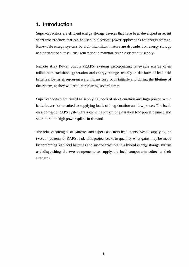
Constant current constant voltage charging (Figure 11) holds current constant for the

first part of the charge until voltage reaches a level where gassing will occur, then the

voltage is held constant and the current allowed to reduce in the same manner as

constant voltage charging [3].

Constant Current Constant Voltage Charging

0

0.5

1

1.5

2

2.5

3

3.5

4

4.5

0 1 2 3 4 5 6 7 8

Time (hr)

Curr

ent (

amps

)

1

1.5

2

2.5

3

3.5

4

Volta

ge (v

olts

)

IV

Figure 11 Constant Current Constant Voltage Charging

Banks of batteries connected in series may have problems after extended cycling due to

small differences in internal resistance and cell capacity [3]. As batteries age resistance

increases and capacity decreases and some cells become worse than others. A weak cell

will be flatter than the others after discharge and require longer to charge. If the

batteries are not fully charged before the next discharge cycle (as is likely with a solar

system) the weak cell will become progressively less charged than its counterparts and

eventually fail. For this reason an equalising charge is recommended every ten cycles or

so [3]. An equalising charge is a charge cycle that lasts longer than usual (usually twice

as long), ensuring that weak cells are returned to full charge [3].

18

3.10 Battery Charging with Photo Voltaics

The output of a solar panel is characterised by its current/voltage or IV curve. Two

characteristic values that are noticeable on an IV curve are the open circuit voltage and

short circuit current. Figure 12 shows on IV curve with a short circuit current of 1.5

amps (voltage = 0) and an open circuit voltage of 14 volts (current = 0).

Solar Panel IV Curve

0

0.2

0.4

0.6

0.8

1

1.2

1.4

1.6

1.8

2

0 2 4 6 8 10 12 14 16

Voltage (volts)

Curr

ent (

amps

)

0

2

4

6

8

10

12

14

16

18

Pow

er (w

atts

)

IVPower

Figure 12 Solar Panel IV Curve

Solar panels were traditionally designed with characteristics similar to Figure 12

because it is well suited to charging a 12 volt battery. Note that the maximum power is

generated at about 12 volts, suiting this panel to supplying a 12 volt system and

charging a 12 volt battery.

Solar cells or photo-voltaic (PV) cells output current in direct proportion to the amount

of sunlight falling on them. Consequently the actual output varies with the day, season

and conditions. To charge batteries control of the output is required and a maximum

power point tracker (MPPT) is often employed.

19

An MPPT is a DC/DC converter that varies its (solar) input current and voltage to keep

the panel operating at the maximum power point, about 12 volts and 1.3 amps in Figure

12 giving a power of about 15 watts.

Batteries require careful control of charging or cycle life is shortened. Excessive over

voltage is particularly damaging to batteries and the resultant gassing increases

maintenance [3]. Batteries used in solar systems must be either over sized so they never

reach full capacity under solar charging [3], or else sophisticated charging control such

as previously mentioned is necessary.

20

4. Super - capacitors

4.1 Background

Capacitors pre-date batteries, being first documented in 1745 [8] and known at the time

as Leyden jars after the university in the Netherlands where they were developed. The

term battery was in fact first used to describe the increased power of a bank of Leyden

jars in the same sense as the increased power of a battery of cannon [8].

Capacitors can be broadly classified as:

• Electrostatic capacitors

• Electrolytic capacitors

• Electro-chemical capacitors

Electrostatic capacitors are typically two metal plates separated by a dielectric as shown

in Figure 13. The strength of the dielectric is measured in volts per metre and defines

the maximum electrostatic field that can exist between the plates without breaking down

[9].

Electrolytic capacitors are similar in construction to electrostatic capacitors. Each plate

has an oxide layer which acts as a dielectric, and the plates are separated by a paper

spacer soaked in electrolyte. The oxide layer is very thin which increases capacitance

per unit volume however the oxide is polarity conscious and will dissolve and short out

the capacitor if the polarity is reversed [9].

Electrochemical capacitors also have an electrolyte solution. Their capacitance is even

greater than electrolytic capacitors due to the porous nature of the electrodes [9].

Super capacitor and ultra-capacitor are the trade names [9] for capacitors also referred

to as electro-chemical double-layer capacitors (EDLC). These capacitors were

developed in the 1960’s [10] and first made commercially available as the Panasonic

Gold capacitor in 1978 [10].

Super-capacitors are grouped into two major categories. Symmetrical super-capacitors

use the same material, usually carbon, for the electrodes. Asymmetrical super-capacitors

21

use two different materials. The electrolyte may be aqueous solutions (such as

potassium hydroxide or sulphuric acid) or organic liquids (such as acetonitrile or

propylene carbonate) [9].

A capacitor stores electrostatic energy, as opposed to a battery which stores chemical

energy and converts it to electrical energy. Electrons are physically added to one plate

of a capacitor and removed from the other when charging or discharging. This means

capacitors can be cycled many times more than batteries (in the order of millions of

cycles) as no physical change occurs within the capacitor during charge and discharge.

4.2 Operation

The classic model of a capacitor is shown in Figure 13. It consists of two plates

separated by a small gap. The gap could be air or some other insulator and is referred to

as the dielectric.

Figure 13 Conventional Capacitor

A discharged capacitor has electrons distributed evenly across the two plates. To charge

a capacitor a potential difference is placed across the capacitor and current flows.

Electrons flow from the positive plate to the negative plate.

+ve Plate -ve Plate

Dielectric

V

+++++++

-------

d

A

22

When charged there is a deficit of electrons on the positive plate and a surplus on the

negative. The total number of electrons within the capacitor has not changed, they are

now concentrated on the negative plate.

This difference in concentration of electrons creates an electrostatic field in the

dielectric between the plates. As current flows the field grows in strength until it is

strong enough to stop current flow. I.e. the potential of the field is equal and opposite to

the applied potential charging the capacitor.

The energy used to charge the capacitor is stored in the electrostatic field. On discharge

current momentarily flows while the electrons redistribute themselves evenly across the

plates. The discharged capacitor has the same number of electrons as the charged

capacitor however they are now spread evenly across both plates.

Capacitance is calculated according to [11]:

Equation 7

Where:

C = Capacitance (Farads)

ε = Dielectric constant, determined by the characteristics of the dielectric

A = the plate area

d = the distance between the plates

Conventional capacitors used in electronics typically have a capacitance in the order of

milli-Farads or less where super-capacitors can achieve capacitance in the order of

thousands of Farads.

Super-capacitors consist of porous electrodes soaked in an electrolyte. When charging a

super-capacitor electrons are physically added to one electrode and removed them from

the other. The ions in the electrolyte separate and accumulate against the electrode of

opposite charge as shown in Figure 14.

dε.AC =

23

Figure 14 EDLC (Super-capacitor)

The porous electrodes have an enormous surface area “A” and the distance “d” between

the electronic charge of the electrodes and the ionic charge of the electrolyte is

incredibly small thereby maximising capacitance “C” according to Equation 7 and

giving super-capacitors a high energy density in comparison to conventional capacitors.

4.3 Capacity

Capacitor voltage varies with energy stored. The energy stored in a capacitor is

proportional to the square of voltage [11]:

2CV21E = Equation 8

The energy delivered to or from a capacitor is given by [9]:

( )22

21 VVC

21ΔE −= Equation 9

Where:

V1 = Initial voltage

V2 = Final voltage

24

Although varying voltage presents a problem to power systems where voltage is kept

constant, the squared relationship means a volt drop of one half delivers three quarters

of the stored energy.

A DC battery-only system operates through a relatively narrow voltage band. A 48 volt

system is likely to operate from 41 volts when flat (assuming a cut off voltage of 1.7

volts per cell, see Figure 4) to around 63 volts while charging at the maximum rate of

2.65 volts per cell.

This voltage range will deliver 56% of a capacitor’s energy, however, in operation the

voltage does not drop from 63 volts to 41 volts when there is a spike in load, instead it

remains relatively constant. In order to deliver a significant amount of energy a DC/DC

converter is required that will maintain a DC voltage equal to battery voltage on the

battery side, and allow the super-capacitor to operate through as wide a voltage as

possible on the capacitor side.

4.4 DC/DC Converters

Figure 15 shows a DC/DC converter as outlined by [12]. Switch S1, diode D1, inductor

L2 and the super-capacitor C form the step down converter that charges the super-

capacitor to just below battery voltage.

Switch S2, diode D2 and inductor L2 form the step up converter that maintains an

output equal to Vbus and allows super-capacitor voltage to operate through a range of

voltages below Vbus.

Capacitor C2 acts a shunt to filter out high frequency ripple which would damage the

super-capacitor.

Figure 15 DC/DC Converter [12].

S1

S2D1

D2

L1

Vbus

_

+

+

Vbat_ L2C1

C2C

25

Due to the small separation of charges super-capacitors can only withstand a relatively

small voltage, in the order of 2.5 volts, without breaking down [9] Exceeding the

maximum working voltage of a super-capacitor can severely reduce its life. In order to

increase voltage to usable levels for applications such as a RAPS system, several super-

capacitors are connected in series. Careful balancing of the voltage across each

capacitor is required to ensure it operates within its voltage tolerance. This can be

achieved passively or actively. Passive balancing uses a balancing resistor in parallel

with each capacitor in the bank to ensure the voltage across each capacitor is equal

however this creates a path for leakage current which will discharge the capacitor bank

over time. Active balancing uses electronics to monitor voltage difference between

adjoining capacitors and actively adjusts the voltage accordingly.

4.5 Fundamentals

Capacitance changes when capacitors are combined in series and parallel. Capacitors

combined in parallel as shown in Figure 16 (a) have a combined capacitance equal to

the sum of their individual capacitances [11]:

n21eq C ... CCC +++= Equation 10

while capacitors combined in series as shown in Figure 16 (b) are combined in the same

fashion as resisters in parallel [11]:

n21

eq

C1 ... C

1C

11C

+++= Equation 11

(a) (b) Figure 16 Capacitors Connected (a) in Parallel and (b) in Series.

Vin Vin

Capacitors in Parallel Capacitors in Series

C1 C2 C3

C1 C2 C3

26

When combining identical capacitors:

Series#Parallel#CC celleq ×= Equation 12

4.6 Internal Resistance

Capacitors, like batteries, have an internal resistance that is modelled as illustrated in

Figure 17. Internal resistance, also referred to as Equivalent Series Resistance (ESR) is

the only efficiency loss associated with super-capacitors [14] and unlike batteries is the

same when charging and discharging.

Figure 17 Simple Capacitor Model

Super-capacitor internal resistance is far less than lead-acid batteries and as a

consequence capacitors are more efficient provided current flow is not excessive.

However because capacitors can discharge (and charge) quickly, the current flow can be

high. Energy loss is an I2R relationship so the internal resistance can become a

significant factor. As with batteries, overall efficiency needs to consider the efficiency

of any electronics, such as DC/DC converters, that operate in conjunction with the

super-capacitor.

Vcap VESR = IR

I

C R

27

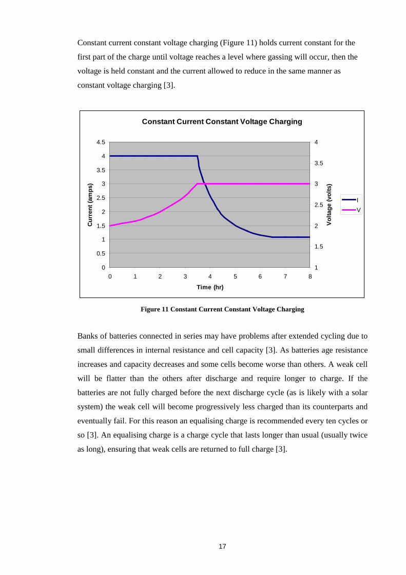
Figure 18 Capacitor Voltage Profile at Constant Current Discharge [13]

The discharge profile of a super-capacitor is shown in Figure 18 [13]. Here:

Vw = working or system DC voltage

VESR = Volt drop due to the Equivalent Series Resistance (ESR)

VCapacitive = Volt drop due to discharging the capacitor

td = Discharge time

The ESR of a typical super-capacitor results in a time constant in the order of one

second [14]. Discharging over shorter periods reduces efficiency and exposing super-

capacitors to continuous ripple current can lead to overheating.

For most applications super-capacitor efficiency is greater than 98% [14] and even

under high current pulse loads, efficiency is greater than 90% [14].

During discharge, super-capacitor voltage varies considerably in comparison to a

battery so a DC/DC converter is required to maintain voltage in a hybrid system which

shares a common DC bus. If connecting to an AC bus a bi-directional inverter with a

wide DC operating range is required. The efficiency of either will contribute to the

overall efficiency of the system.

time

volta

ge.

VESR

VCapacitive

28

4.7 Capacitor Life

A super-capacitor is considered to have reached the end of its life when either its

capacitance drops by 20% or its internal resistance increases 100% [15]. However in

practice end of life is when the device is no longer capable of performing the task it was

designed for. Super-capacitors are capable of being cycled millions of times before a

significant reduction in capacitance or increase on resistance is apparent. Figure 19 [14]

shows decrease in capacitance for cycles at different operating voltages. Each charge

and discharge cycle is followed by a 15 second rest [14].

Figure 19 Capacitance Decrease while Cycling at Different Voltages [14]

The number of cycles a super-capacitor can perform before their end of life is reached

depends on operating temperature and the maximum cell voltage. Testing shows super-

capacitor life of ten years at nominal operating temperature (25°C) at a voltage of 3.0

volts (0.5 volts above nominal) or a life of ten years at nominal voltage (2.5 volts) at a

temperature of 65°C [16]. At nominal voltage and temperature, the same capacitor

would be expected to have a life of one hundred years [16].

29

4.8 Temperature Effects

Low operating temperatures increase super-capacitor internal (ESR) resistance to

varying degrees depending on the electrode and electrolyte type [16] Low temperature

can also reduce capacitance [16]. Figure 20 [14] shows the change in capacitance and

internal resistance over the operating temperature range of a super-capacitor.

Figure 20 Capacitance and Internal Resistance Variation with Temperature [14]

30

5. Strengths of Lead Acid Batteries and Super-capacitors

Figure 21 [17] shows a Ragone plot of various energy storage technologies. The

characteristics to note are that batteries are high in energy density and deliver energy in

the order of hours where super-capacitors (Double Layer Capacitors and Ultra-

capacitors) while lower in energy density are higher in power density and deliver energy

in seconds.

The combined strength of these two technologies is to use batteries to support loads of

long duration and low power demand and super-capacitors for loads of short duration

and high power demand such as would be expected of a RAPS system with a normal

domestic load.

Figure 21 Ragone Plot of Energy Storage Devices [17]

31

6. Data Collection Previous investigations [12] [18] have shown that a hybrid super-capacitor lead acid

battery energy store is viable for RAPS systems. These studies have used a variety of

load profiles to simulate the energy store behaviour including pulsed loads and weekly

load profiles.

This investigation seeks to use real load data sampled at a rate of one sample per second

from an existing RAPS system to gain an accurate indication of typical loads and

quantify what gains may be made.

6.1 The RAPS System

A RAPS installation near Boyup Brook approximately 300km south east of Perth was

monitored for one week in early September 2010. The system was installed by WA

Solar Supplies in 2005.

The site is approximately three kilometres through bushland to the grid. Estimated cost

of connecting to the grid at the time was $75 000 with extra required to clear a path

through the bushland for the line.

The owners did not want to clear native vegetation as part of their reason for living there

was the bush environment which they did not wish to damage.

32

The system cost approximately $90 000 with a rebate from the government at the time

of about $42 000. Total cost to the owners was in the vicinity of $48 000. Even without

the rebate the RAPS system would have been a viable alternative to connecting to the

grid.

This system comprises a 2.4kW array of thirty BP485 BP Solar 85W nominal (80W

guaranteed) mono-crystalline solar panels, as shown in Figure 22.

Figure 22 2.4kW Solar Array

33

Energy storage is a bank of eight Magnum Premium six volt wet cell deep cycle lead

acid batteries of 875Ah capacity at the C100 rate, shown in Figure 23. These batteries

have a design life of seven years. The cycle life versus DOD plot was shown in Figure 5

and an estimation of the battery capacity at varying discharge rates in Figure 2.

Figure 23 48 Volt Battery Bank

34

An eleven kVA diesel generator (Figure 24) provides backup power. The generator

control starts the generator once a fortnight to charge the batteries to 100% SOC and

equalise cell voltages. The generator starts in overload situations and if the battery SOC

falls below a set point, say 50% (not confirmed).

Figure 24 11kVA Generator

35

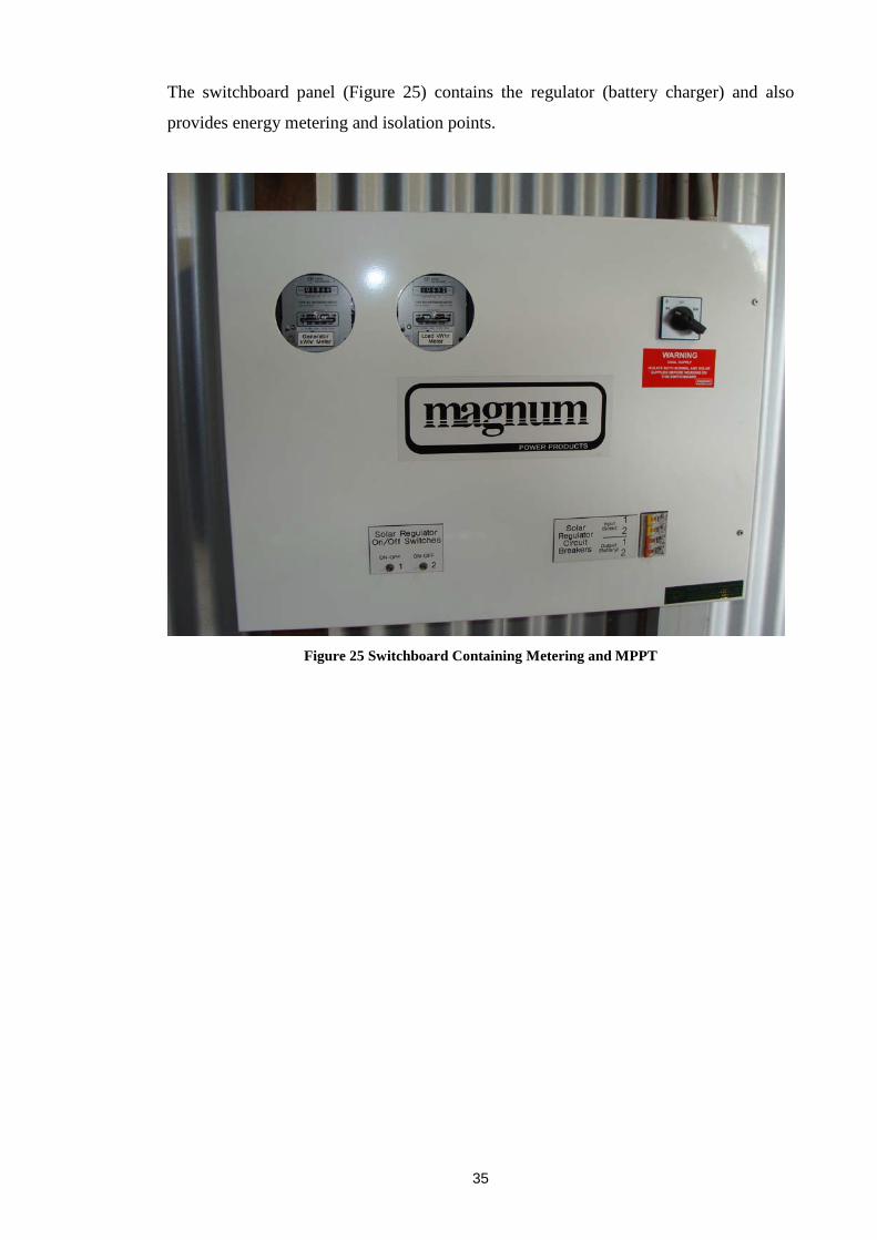
The switchboard panel (Figure 25) contains the regulator (battery charger) and also

provides energy metering and isolation points.

Figure 25 Switchboard Containing Metering and MPPT

36

The inverter (Figure 26) is also the system controller, monitoring battery condition, load

and dispatching the generator as required.

Figure 26 Inverter and System Controller

37

Data was collected at the AC input to the switchboard as shown in Figure 27. The

power meter was a Yokogawa CW240 clamp on power meter which was kindly lent by

Murdoch’s RISE institute for use on this project.

Figure 27 Data Collection

38

6.2 The Data Taker

The current clamp can be seen at the top of Figure 27. The orange lead is the voltage

reference for the meter and the black lead is the battery charger. The meter has enough

battery backup for about half an hour of operation if the power fails.

Current was sampled at a rate of once a second. The data was saved as .csv files and

analysed in Microsoft Excel. Data validation showed occasional glitches (approximately

one in nine thousand data points) when data was lost and columns of data became

misaligned. This made the problems easy to spot and rectify. The missing data ranged

between one and two seconds. In each case the preceding one or two seconds of data

was copied in to create complete data sets.

6.3 The Data

Figure 28 is a sample of load from the morning of Saturday the 4th of September 2010.

The occupants of the house documented their appliance use during the monitoring

period. The first 4 amp pulse in load appears to be the toaster. The second pulse from 2

to 4 amps with the large spike to almost 12 amps is probably the water pump. The pulse

to 12 amps just before 9:30 is the kettle and the regular spikes that start just before 9:40

is the bread maker.

Figure 28 Load Profile 04 September 2010.

Morning Load Profile

0.00

2.00

4.00

6.00

8.00

10.00

12.00

14.00

8:50:00 9:00:00 9:10:00 9:20:00 9:30:00 9:40:00 9:50:00 10:00:00

Time

Amps

39

7. Matching Super-capacitors to Load The load profile shown in Figure 28 has an underlying base load of close to 2 amps with

interspersed pulses of varying amplitude and duration. The relative strengths of batteries

and super-capacitors suggests that the base load would be best met by lead-acid

batteries while the pulses in load would be better met by super-capacitors.

Before progressing further it is appropriate to assess when this load is “seen” by the DC

side of the RAPS system.

In normal operation the load is met by solar generation and only supplied by the

batteries when generation drops below demand or ceases altogether.

For simplicity consider conditions at the RAPS site are such that at noon rated solar

output is reached and being September and close to the equinox solar generation is from

6:00AM until 6:00PM. The solar array at the site is rated at 2.4kW which (ignoring

losses) equates quite nicely to ten amps maximum output after converting to 240 volts.

PV Output and Load

0

2

4

6

8

10

12

14

0:00:00 6:00:00 12:00:00 18:00:00 0:00:00

Time

Amps

(AC

equi

vale

nt)

Figure 29 Daily Load and Daily Solar Production.

Note in Figure 29 that solar output is shown by the pink line and load by the yellow. All

load falling under the pink line is met by the solar generation and never “seen” by the

energy storage.

40

To utilise super-capacitors to their advantage (short bursts of high energy) only those

spikes in demand that exceed the solar generation will be met. In order to meet the next

spike in demand the super-capacitors need to be charged as soon as practicable after use

which impacts the charging dispatch: the super-capacitor must be charged first (before

the battery) when excess generation is available.

When there is no excess generation available the super-capacitor must either have

enough capacity to last until the next day, recharge from the batteries or not be utilised.

7.1 Super-capacitor Sizing

Super-capacitor sizing as outlined in [12] assumes sizing the capacitor to cover direct on

line motor starting loads of less than one second duration. Analysis of the collected data

shows there are many spikes in demand of durations up to two minutes that can be met

by super-capacitors. In addition capacitors and inductors within the inverter are likely to

filter out spikes of only a few cycles duration and as such they won’t be “seen” by the

DC side of the system.

As a starting point a super-capacitor can be sized to a load such as the kettle as shown

in Figure 28. Recall energy delivered is proportional to the square of voltage. When a

capacitor delivers energy the voltage drops. To maintain a DC bus voltage of 48 volts a

DC/DC converter such as shown in Figure 15 would be required to incorporate

capacitors.

Assume the DC/DC converter covers a range of 48 – 24 volts on the capacitor side, and

a constant 48 volts on the battery side.

Recall an amp second is a Coulomb. The energy stored by a capacitor can equally be

written as [11]:

2Cq E

2

= Equation 13

41

where:

E = Energy (Joules)

q = Charge (Coulombs)

C = Capacitance (Farads)

The power used by the kettle is therefore [11]:

secondJoules 2400 Watts2400 P

10 240 P

VI P

==

×=

=

Equation 14

The kettle ran for two minutes = 120 seconds. The energy used by the kettle is therefore

[11]:

Joules 000 288 E

120 2400 E

tP E

=

×=

×=

Equation 15

Rearranging Equation 9 to solve for capacitance we have:

( )

( )

Farads 333.33 C

2448000 288 2 C

VV2E C

22

22

21

=

−×

=

−=

Equation 16

Choose a suitable capacitor from the Maxwell ultra-capacitor range, say the BCAP2000

P270 T05 2000 Farad capacitance with an ESR of 0.35mΩ and a rated voltage of 2.7

volts [19]. To ensure capacitors do not exceed operation voltage [13]:

42

seriesin Cells 18Say

17.7Seriesin Cells#

2.7V48VSeriesin Cells#

Voltage CellVoltage SystemSeriesin Cells#

=

=

=

Equation 17

From Equation 12 capacitance now equals:

Farads11.111C

1812000C

Series#Parallel#CC

eq

eq

celleq

=

×=

×=

Equation 18

In order to meet the kettle load we require 333.33 Farads.

capacitors-ultra 18 of Strings 3Parallel#

200018 33.333Parallel#

CSeries# C

Parallel#

Series#Parallel#CC

cell

eq

celleq

=

×=

×=

×=

Equation 19

43

To check performance internal resistance is now:

0.0021ΩR

3180.00035R

Parallel#Series#RR

eq

eq

celleq

=

×=

×=

Equation 20

Calculate the average current flowing through the capacitor [13]:

Amps 100I

242400I

VPI

max

max

minmax

=

=

=

Equation 21

Amps 50I

482400I

VPI

min

min

maxmin

=

=

=

Equation 22

Amps 75I

250100I

2III

ave

ave

minmaxave

=

+=

+=

Equation 23

44

The average VESR volt drop according to Figure 18 would be:

Volts 5157.0V

0.002175 V

IR V

=

×=

=

Equation 24

And the actual energy delivered by the capacitor:

( )

( )( )

Joules 484 285 E

241575.04833.33321 E

VVC21 E

22

22

21

=

−−×=

−×=

Equation 25

Recall the kettle required 288 000 Joules. There is a shortfall of 2516 Joules. The volt

drop due to ESR is small: 0.3% of maximum working voltage. However due to the

squared relationship with voltage the energy delivered has been reduced by almost 1%.

Consider also that inefficiencies of converters and losses in conductors have not been

accounted for. A larger capacitance is called for.

45

8. RAPS System Model Two simulation packages were considered to model the RAPS system, the Matlab

package Simulink or PSpice circuit simulation software. Simulink was chosen as it has

the capacity to handle large data sets and is suited to iterative calculations which are

required for SOC and battery temperature calculations.

The Simulink model was created to capture gains that may be achieved by

implementing a battery/super-capacitor hybrid energy storage system and utilising their

relative strengths i.e. batteries supply long duration base load and super-capacitors

supply short duration spikes in load.

The model is designed to capture gains in battery SOC, battery temperature, battery

efficiency and system efficiency and as such consists of four major components.

The advantages of this model are in having real load data against which to simulate

battery performance. Additionally parameters such as internal resistance, battery

capacity and physical size can be easily adjusted to model different products or to tune

the model to test data when available.

The main disadvantage of the model is that due to the size of the load data files a one

week simulation takes several minutes to run. RAPS systems typically operate for

decades, so a lifetime simulation was not possible. This model is highly dependent on a

one week data set being representative of decades of operation.

8.1 State of Charge (SOC)

Battery SOC can be calculated by integrating net current flow through the battery [1].

The difficulty lies in the fact that battery capacity diminishes with increased rate of

flow. There are two options to account for the diminished capacity, use data sheets to

determine Peukert’s equation or calculate losses due to internal resistance.

To calculate battery SOC using Peukert’s equation, assume that the battery capacity

remains static at the nominal battery capacity “C” rate (875Ah). Current flow can then

46

be scaled to the equivalent rate that would achieve the same charge or discharge at this

capacity.

Battery capacity at any given current flow rate can be calculated from the Peukert

equation determined in Figure 2. This equation was estimated from typical battery data

and fitted to the Magnum battery used in the monitored RAPS system. The data sheet

for the magnum battery gave only two “C” rate capacities, C10 = 660Ah and C100 =

875Ah.

The battery capacity at any given discharge rate has been determined as:

14.0dI5.1185C −×=

Equation 26

To illustrate a discharge rate of twenty amps would result in a capacity of 779Ah

according to Equation 26. Nominal capacity is 875Ah so the equivalent SOC would be

reached by discharging at:

22.46 I

779875 20 I

CC I I

eq

eq

actual

nominaleq

=

×=

×=

Equation 27

If there were no losses (Peukert effect) discharging at 20 amps from a 779Ah battery

would be the equivalent of discharging at 22.46 amps from an 875Ah battery.

Battery SOC is calculated by integrating the current flow over time. The current flow

data has a one second sample time rate. The integral of current flow is therefore

amp.seconds (coulombs):

∫××=t

0I(t)

3600sec1hr

(Ah)Capacity Battery %100 %SOC(t) dt Equation 28

47

This is achieved in discrete time as:

I(t)3600sec

1hr(Ah)Capacity Battery

%100 %SOC(t) 1)%SOC(t ××+=+ Equation 29

This has been implemented in Simulink as in Figure 30:

Figure 30 Simulink Battery Model

8.2 Internal Resistance

Internal resistance is not available on the manufacturer’s data sheets. Internal resistance

is required to model heat generation and can be used as an alternative to Peukert’s

equation to capture losses that normally occur when charging and discharging a battery

creating the loss of capacity phenomena.

Using internal resistance allows a model that has different charge and discharge

characteristics, an improvement on using Peukert’s equation which is determined for

discharge only.

+

_ 1/3600

+

+

1Z

x

÷100SOC

875

BatterySOC

BatteryCapacity (Ah)

Gain

Unit Delay

Gain

ToWorkspace

Net BatteryCurrent

Heat losses

Battery Ah (nom)

Battery Ah (actual)

48

The losses are realised by calculating the equivalent current that has been lost to heat

generation and subtracting it from the value to be integrated to calculate SOC. In effect

charging current is reduced and discharging current is increased in SOC calculations

due to heat generation.

8.3 Heat Generation and Battery Temperature

There are two contributions to heat generation within a battery, joule heat generation

and heat generated by the chemical reactions. Joule heat generation is exothermic when

charging and discharging while heat from chemical reactions is exothermic while

charging and endothermic while discharging. According to [20] joule heat generation

dominates for all except long periods of very low discharge (not expected in this

application) and so has been ignored in the simulation.

In addition water decomposition into hydrogen and oxygen is a loss in efficiency with

heat consequences. In a vented cell the gas carries away the energy used to create it

however gas production increases electrolyte resistance and increases polarisation

which adds to joule heat generation.

Joule heat generation is realised in the model as I2R, where I is the charge or discharge

current and R is the internal resistance. This is achieved in the model by switching to

the charge resistance when battery current is positive and switching to the discharge

resistance when battery current is negative.

A higher internal resistance value has been used for charging than discharging on the

basis of heat generation discussion in [1] and higher values chosen in the model done by

[21] which was verified against test data. [21] uses a value nearly twice discharging

resistance for a VRLA battery. As this model is for vented cell batteries which do not

generate heat recombining oxygen so a value 1.7 times discharge resistance has been

chosen.

Heat generation (in watts, Figure 31) is modelled as I2Rohmic where:

R = 0.025Ω when discharging

R = 0.0425Ω when charging

49

This is a compromise on actual internal resistance as it is dependent on many variables

and varies with time depending on battery SOC and usage history.

Discharge resistance was chosen by creating two models, one using Peukert’s equation

to calculate discharge characteristics, and the other (as shown) “tuned” to the same

response by varying the discharge resistance until the same discharge curve was

achieved.

Figure 31 Simulink Heat Generation Model

The current that does not contribute to charging (losses) is calculated by dividing the

heat (in watts) by battery voltage to obtain heating amps. Heating amps are then

subtracted from battery current before integrating to calculate SOC.

U2 0.0425

Charge

Net BatteryCurrent

Heating watts

0.025

Discharge

>=0

x

÷

Heatlosses

6

Batteryvoltage

Compare to zero

I squared

Heatingamps

50

Battery temperature is a function of heat generation and heat dissipation. Heat is

generated by current flow through the battery internal resistance and is given by:

ohmic2

in RIq = Equation 30

Where:

q = Heat flow rate in joules per second (watts)

I = Current flow in amps

Rohmic = Electrical resistance in ohms

Temperature change depends on thermal capacity and the flow of energy into or out of a

body [22]. The thermal capacitance of a battery (Cbatt) determines how much a given

amount of energy will change a body’s temperature. Cbatt has the units of joules per

kelvin and can be determined from a body’s specific heat (Cp, kilojoules per kilogram

kelvin) and mass (M, kilograms) by [22]:

Cbatt = MCp Equation 31

Flooded cell lead acid batteries have a specific heat of just over 1 kJ/(kg.K) [2]

depending on type and construction while VRLA batteries have a Cp of 0.7 to 0.9

J/(kg.K) [2].

The change in a body’s temperature (T) is determined by [22]:

( )dt∫ −= qq

C1ΔT outinbatt Equation 32

Therefore the battery temperature at time t is given by [22]:

( )dtt

(t)q(t)qMC

1TT(t)

0 outinp

initial ∫ −+= Equation 33

51

Heat dissipation is proportional to the difference in temperature between a body and its

surroundings and dependant on the thermal resistivity (Rthermal, kelvin seconds per joule

or kelvins per watt) of the substance separating them [22]:

( )airbatterythermal

out TTR

1q −= Equation 34

The thermal conductivity (α, watts per metre kelvin) of plastics used for battery cases is

0.2 W/(m.K) [2]. For a separating substance of cross sectional area A and thickness d

thermal resistivity can be determined by [22]:

d

AαR

1

thermal

×= Equation 35

Heat dissipation from a battery is mainly through the sides as the bottom is usually in

contact with the ground which attains the same temperature as the battery, and the lid is

separated from the electrolyte by a layer of air which is a poor conductor of heat [1]

The temperature of the battery can therefore be determined by [22]:

( ) dt (t)T(t)Td

AαRI(t)MC

1T(t)T airbatteryohmic2

pinitialbattery ∫

−

×−+=

Equation 36

This is achieved in discrete time as:

( ) 1)(tT1)(tTd

AαR1)I(tMC

1(t)T1)(tT airbatteryohmic2

pbatterybattery

+−+

×−++=+

Equation 37

This has been implemented in Simulink as in Figure 32:

52

Figure 32 Simulink Battery Temperature Model

+

_

+

+

1Zx

÷

0.004

Temp

BatteryTemp

ToWorkspace

Unit Delay

Battery WallThickness

Heatingwatts

X

Batterymass

133

Constant

1

X

Battery HeatCapacity

1000

1/MCp

X

x÷1/R

0.2

ThermalConductivity

0.922

SurfaceArea

X

25

Ambientair temp

+_

53

8.4 Load and Battery Current

The load data collected from the RAPS system was used to create Matlab .m files

named Sunday.m through to Saturday.m. Once run in the Matlab workspace they can be

called by Simulink via the Load Profile block which runs a separate Simulink model

called Wildy Load to generate one week of load data points with a one second time step.

The solar generation is approximated using the positive values of a sine wave generator.

As the load data collected represents the AC load, for simplicity, solar generation was

modelled as AC current. I.e. 2.4kW solar array would produce 10 amps when converted

to 240 volt AC (ignoring losses) at rated production.

The Generator Control block (Figure 33) is an embedded Matlab code which dispatches

the generation according to load and battery condition:

• When there is solar generation and the battery is not fully charged the entire

solar production is output. If the battery is fully charged only the solar

generation equal to the load is output.

• If the battery reaches 50% SOC, the generator is dispatched until the battery is

fully charged. There is also the ability to dispatch the generator at predetermined

time intervals utilising the Counter Limited block.

The PV and Diesel current blocks are outputs to the Matlab workspace which allow the

PV and Diesel production to be analysed.

54

Figure 33 Simulink Load and Generation Model

10

Sine Wave

>=0

Generator

Compare to zero

X

Load Profile

Wildy Load Out 1

++

PV

Diesel

ToWorkspace

ToWorkspace

CounterLimited

15

+

_

Convert to DC amps

5

u6

u1

u2

u3

u4

u5

y4

y3

y2

y1

fcn

GeneratorControl

Load

Generation

BatteryAh (nom)

5

Load (to Capacitor control)

Net DCCurrent

Battery Ah (actual)

55

8.5 The Capacitor

The capacitor is implemented in the same manner as the battery and the same SOC

calculations apply, however no losses have been included in the capacitor model. The

capacitor has its own control block which is an embedded Matlab code. Assuming no

losses the load data generated by Wildy Load is scaled to DC current by:

ACDC

ACDC

ACDC

ACDC

I5I

I48

240I

IVVI

×=

×=

×=

Equation 38

The base load block outputs the minimum value from the input vector “u” and is reset

by a logic value of one at the input “R”. The Counter Limited block cycles to zero every

3600 time steps i.e. every hour. The rationale is that the one hour minimum value

represents the base load. Significant deviations (one amp) above this represent spikes in

loads the capacitor will supply.

The Capacitor control block (Figure 34) compares net DC current to the value returned

by the base load block. If the capacitor is greater than 25% charged then loads greater

than one amp above the base load input are supplied by the capacitor.

If the capacitor is less than 100% charged and battery current is positive (i.e. it is

charging) the capacitor is charged from the net DC current. If the capacitor is less than

100% charged and the battery current is negative (i.e. it is discharging) the capacitor is

not charged. In this way the capacitor is only charged when there is generation

available.

The switches (Figure 34) allow the capacitor to be isolated from the system and

simulate battery only operation.

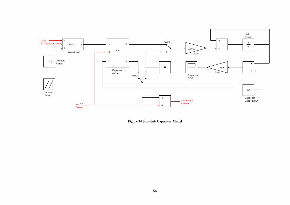
56

Figure 34 Simulink Capacitor Model

0

1/3600

+

+

1

Z

x

÷100

80

CapacitorSOC

CapacitorCapacity (Ah)

Gain

Unit Delay

Gain

Net BatteryCurrentNet DC

Current

Switch

fcn

u3

u1

u2

y2

y1

Capacitorcontrol

+

+

SwitchMin (u,y) y

R

u

Base Load

Load (to Capacitor control)

CounterLimited

Compare to zero

= = 0

8.6 Modelling Issues

Several issues arose during the development of the model. The first was the volume of

data produced by monitoring. Microsoft Excel 2003 could only handle twelve hours of

data on one page and plots had to be broken down into six hour series.

Matlab could not process more than one day of data in one .m file. Load data was

created in .m files for each day Sunday to Saturday inclusive. Because the load data

produced by the .m files was time stamped it was not easily cycled to simulate more

than one week of operation. A solution was presented but not implemented for this

study.

Initially the model used a sinusoid to simulate varying temperature around a mean of

25°C throughout the day. However, for comparison purposes, it was decided to remove

variability and maintain 25°C ambient temperature as a standard operating condition for

the duration of all simulations.

Implementing a constant in place of the sinusoid caused Matlab to terminate simulations

and flag an error message. The reason was not investigated as the varying temperature

function could be retained for other simulations and setting a negligible sinusoid

amplitude of 0.01 while maintaining the 25°C mean was deemed to be suitably accurate.

Several control methods have been trialled for dispatching the capacitor with various

levels of impact. With more attention to control, for example proportional or

proportional integration controller more accurate representation may be made. Charging

the capacitors slowly from the batteries when no generation is available was trialled

however the gains were not as great as generation only charging.

For simulations the generator output was set to zero as a standard operating condition.

For simulations of greater than two weeks the generator may be implemented as the

monitored system ran the generator once a fortnight to ensure the batteries were 100%

charged. Potential savings in diesel could then be calculated.

58

9. Simulation Results As the hours of sunlight vary throughout the year the dependence on stored energy also

varies. An operational scenario of equal hours of daylight and darkness could be

considered representative of the average system behaviour and indicate the suitability of

a lead-acid battery super-capacitor energy store. Simulations were run with the capacitor

bank increasing in size while the battery bank was reduced by the same amount

maintaining total energy storage at 875Ah.

An optimum super-capacitor size was determined by the greatest average battery SOC.

This size of super-capacitor was then held constant and the battery size reduced until a

battery was found that would give the same cycle life as the battery only case.

Monitored parameters were average PV generation (amps), average battery input and

output current (amps), average battery SOC (%), average battery DOD (%), maximum

battery temperature (°C) and average battery temperature (°C).

Average SOC was calculated as the average of all SOC values, where as average DOD

was calculated from the average of the minimum SOC values.

Diesel generation was set to zero and ambient temperature to 25°C as standard test

conditions. This was done to reduce variability between simulations. A constant

ambient temperature provides a base to compare battery temperature to. The diesel

generator was disabled because it added complexity to what was already a busy

simulation and removing it reduces complexity when comparing simulations. Analysing

solar generation alone provides adequate insight into system behaviour over a one week

simulation.

The base case is the battery only storage system. Net battery current is shown in Figure

35. Negative values are battery discharge current and positive values battery charge

current. Quite apparent are the spikes in load (below zero).

59

Figure 35 Base Case Battery Only: Net Battery Current

The y axis displays battery current in amps and the x axis time in seconds ×104. Time

zero is midnight. At time 21 600 (6:00 AM) battery current goes positive due to solar

generation. Load is met by solar generation when it is available. The dips in battery

current correspond to load greater than solar generation and so battery energy is also

required. At around time 46 800 (1:00 PM) current drops to zero as the battery is fully

charged and load is met by the generation. In the evening load is greater than generation

and the battery is used again with solar generation ceasing at time 64 800 (6:00 PM).

Note midnight is at time 86 400. The plot extends into the early hours of the next day.

60

By comparison, with the addition of a super-capacitor the battery discharge current is

relatively constant or zero as shown in Figure 36 for one day of simulation.

Figure 36 Optimum Case with 65Ah Capacitor: Net Battery Current

The y axis displays battery current in amps and the x axis time in seconds ×104. Time

zero is midnight. At time 21 600 (6:00 AM) solar generation commences however this

is not seen by the battery as the super-capacitor is charged first. The super capacitor is

fully charged at around time 28 800 (8:00 AM) when battery current suddenly jumps to

20 amps. The battery is charged until about time 36 000 (10:00 AM) when it is fully

charged and current falls to zero. Load is met by solar generation when it is available. In

the evening load is greater than solar generation and the battery is used again with solar

generation ceasing at time 64 800 (6:00 PM). After this time super-capacitor is meeting

all the spikes in load (negative current) and the battery is meeting base load close to

negative 10 amps before dropping to zero around time 88 200 (12:30 AM).

Note midnight is at time 86 400. The plot extends into the early hours of the next day.

61

Figure 37 shows the super-capacitor discharge current for the corresponding period.

Note the spikes in current visible in Figure 35 are now flowing through the super-

capacitor.

Figure 37 Optimum Case with 65Ah Capacitor: Net Capacitor Current

The y axis displays battery current in amps and the x axis time in seconds ×104. Time

zero is midnight. At time 21 600 (6:00 AM) super-capacitor current goes positive due to

solar generation. The super-capacitor is charged first so it can be available for the next

spike in load. The dips in super-capacitor current correspond to load greater than solar

generation. At around time 28 800 (8:00 AM) current drops to zero as the super-

capacitor is fully charged and load is met by the generation. Shortly after at about time

32 400 (9:00 AM) load exceeds generation and both the super-capacitor and the battery

(see Figure 36) are called on to meet the load. Note the super-capacitor is discharged

(negative current) far more than the battery. Current then falls to zero as the load is met

by generation. In the evening load is greater than generation and the super-capacitor is

used again with solar generation ceasing at time 64 800 (6:00 PM).

Note midnight is at time 86 400. The plot extends into the early hours of the next day.

62

The battery SOC for the period of the simulation (one week) is shown in Figure 38.

Every day the battery is fully charged and discharges to around 90% and in fact the

average of the minimum values is 90% equating to an average DOD of 10%.

Figure 38 Base Case Battery Only: Battery SOC

The y axis represents battery SOC in % while the x axis is time in seconds ×105. The

battery starts and ends the simulation at the same SOC allowing battery efficiency to be

calculated. Battery SOC reaches 100% at around midday each day and drops from the

end of solar generation at 6:00 PM. Minimum SOC is reached just before solar

generation commences at 6:00 AM.

63

By comparison with the addition of super-capacitors the battery SOC ranges from fully

charged to about 95% charged (Figure 39). The average of the minimum values is

94.3% equating to and average DOD of 5.7%. The improvement in average DOD

between the battery only option and 65Ah capacitor was 4.3%.

Figure 39 Optimum Case with 65Ah Capacitor: Battery SOC

The y axis represents battery SOC in % while the x axis is time in seconds ×105. The

battery starts and ends the simulation at the same SOC allowing battery efficiency to be

calculated. Battery SOC reaches 100% at around midday each day and drops from the

end of solar generation at 6:00 PM. Minimum SOC is reached just before solar

generation commences at 6:00 AM.

64

Battery temperature for the simulation period peaked while charging, mostly just over

26°C with small increases during the discharge period as shown in Figure 40.

Figure 40 Base Case Battery Only: Battery Temperature

The y axis represents battery temperature in °C while the x axis is time in seconds ×105.

The peaks over 26°C correspond to temperature rising during charging until the battery

is fully charged and battery current falls to zero. At this point battery temperature drops

as heat is dissipated to the surroundings. The minor rise in temperature following each

major peak corresponds to battery discharge while the load is still reasonably high just

after solar generation ceases at 6:00 PM. As the load drops away around midnight the

battery cools to ambient temperature which was held constant at 25°C.

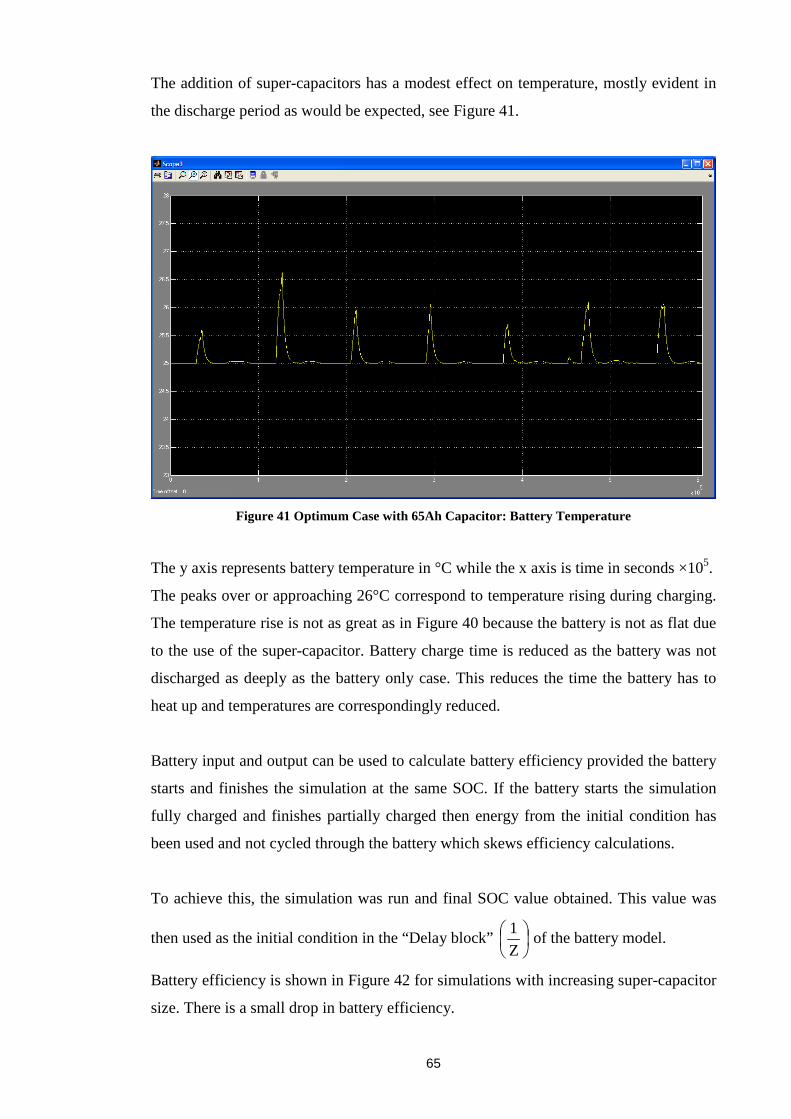
65

The addition of super-capacitors has a modest effect on temperature, mostly evident in

the discharge period as would be expected, see Figure 41.

Figure 41 Optimum Case with 65Ah Capacitor: Battery Temperature

The y axis represents battery temperature in °C while the x axis is time in seconds ×105.

The peaks over or approaching 26°C correspond to temperature rising during charging.

The temperature rise is not as great as in Figure 40 because the battery is not as flat due

to the use of the super-capacitor. Battery charge time is reduced as the battery was not

discharged as deeply as the battery only case. This reduces the time the battery has to

heat up and temperatures are correspondingly reduced.

Battery input and output can be used to calculate battery efficiency provided the battery

starts and finishes the simulation at the same SOC. If the battery starts the simulation

fully charged and finishes partially charged then energy from the initial condition has

been used and not cycled through the battery which skews efficiency calculations.

To achieve this, the simulation was run and final SOC value obtained. This value was

then used as the initial condition in the “Delay block”

Z1 of the battery model.

Battery efficiency is shown in Figure 42 for simulations with increasing super-capacitor

size. There is a small drop in battery efficiency.

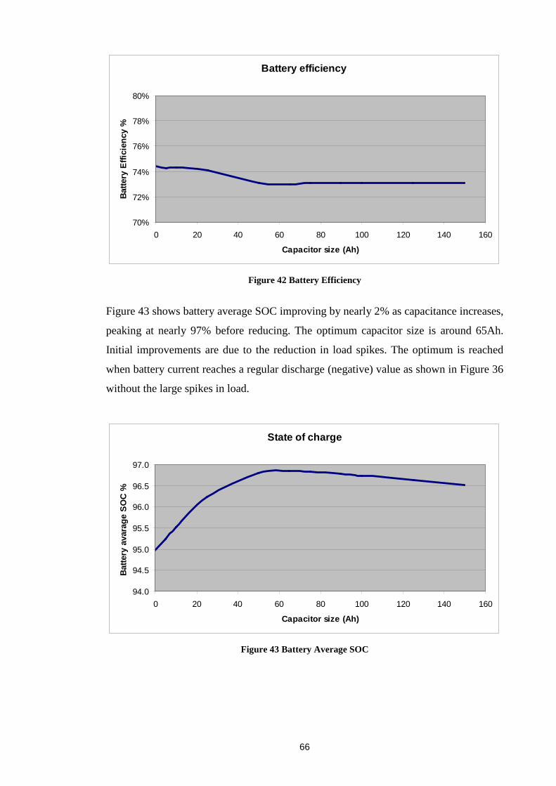
66

Battery efficiency

70%

72%

74%

76%

78%

80%

0 20 40 60 80 100 120 140 160

Capacitor size (Ah)

Batte

ry E

ffici

ency

%

Figure 42 Battery Efficiency

Figure 43 shows battery average SOC improving by nearly 2% as capacitance increases,

peaking at nearly 97% before reducing. The optimum capacitor size is around 65Ah.

Initial improvements are due to the reduction in load spikes. The optimum is reached

when battery current reaches a regular discharge (negative) value as shown in Figure 36

without the large spikes in load.

State of charge

94.0

94.5

95.0

95.5

96.0

96.5

97.0

0 20 40 60 80 100 120 140 160

Capacitor size (Ah)

Batte

ry a

vara

ge S

OC

%

Figure 43 Battery Average SOC

67

Current flow into (charging) and out of (discharging) the battery decreases with

increasing super-capacitor size. Figure 44 shows average battery charge and discharge

current decreasing by 49% with the optimum super-capacitor size being about 70Ah.

Average Battery Current

0

1

2

3

4

5

6

0 20 40 60 80 100 120 140 160

Capacitor size (Ah)

Curr

ent (

amps

)

Current InCurrent Out

Figure 44 Average Battery Current

Overall system efficiency was calculated from total generation input versus total load.

As shown in Figure 45, efficiency improved by around 8% with the inclusion of

capacitors. The optimum capacitor size is around 80Ah.

Overall Efficiency

85%

86%

87%88%

89%

90%

91%92%

93%

94%

0 20 40 60 80 100 120 140 160

Capacitor size (Ah)

Effic

ienc

y %

Figure 45 System Efficiency

68

As efficiency increased the average PV current decreased from 1.82 to 1.68 amps as

shown in Figure 46. This represents a 7.7% decrease in PV current and therefore energy

required from the generation. The optimum super-capacitor size is around 80Ah.

PV Output

1.66

1.68

1.71.72

1.74

1.76

1.781.8

1.82

1.84

0 20 40 60 80 100 120 140 160

Capacitor size (Ah)

Aver

age

Curr

ent (

amps

)

Figure 46 Average PV Current

69

There is a modest reduction in temperature, both average temperature during the

simulation (Figure 47) and maximum temperature (Figure 48).

Average Temperature

25

25.1

25.2

25.3

25.4

25.5

0 20 40 60 80 100 120 140 160

Capacitor Size (Ah)

Tem

pera

ture

(deg

C)

Figure 47 Average Temperature

Maximum Temperature

26

26.4

26.8

0 20 40 60 80 100 120 140 160

Capacitor size (Ah)

Tem

pera

ture

(deg

C)

Figure 48 Maximum Temperature

70

The optimum super-capacitor size of 65Ah was identified as the best match to improve

battery SOC. This super-capacitor size was held constant and battery size reduced until

a battery size was found that would have the same average DOD as the battery only

case. Figure 49 plots the average DOD. Recall the battery only case had a DOD of 10%

indicating a 460Ah battery would give the same cycle life.

Fixed Capacitor 65Ah

7

8

9

10

11

12

13

14

340 360 380 400 420 440 460 480 500 520 540 560

Battery capacity (Ah)

Aver

age

Batte

ry D

OD

%

Figure 49 Spring Case: Fixed Super-capacitor Variable Battery

71

10. Discussion

10.1 The Problem

RAPS systems incorporating renewable energy by nature require energy storage to

provide energy during periods when generation is less than demand. Lead-acid batteries

are a common choice because they are readily available, well understood and

affordable. However lead-acid batteries are often considered the weak point in a RAPS

system because they represent a significant financial outlay, can be inefficient and

require replacing several times during the life of a RAPS system.

The initial assumption for this study was that there were gains to be made utilising the

strengths of lead acid batteries and super-capacitors by using the super-capacitors to

supply transient spikes in load and batteries to supply base load.

This investigation seeks to:

• Record and analyse a typical RAPS load to verify the load profile.

• Simulate an energy storage system that supplies the transient loads with super-

capacitors and the base load with batteries.

• Find the optimum size for the super-capacitor.

• Quantify the improvements in battery and system performance.

• Investigate the feasibility of a proposed hybrid system.

10.2 The Investigation

The first step was to verify the nature of the load on a real RAPS system. To that end a

RAPS system was monitored and analysis of the data verified that an assumption of

base load suited to batteries with transient pulses and spikes in load suited to super-

capacitors was reasonable. The data was validated and saved into an appropriate format

to be used in a simulation of a RAPS system incorporating a hybrid super-capacitor

lead-acid battery energy storage unit.

There are two types of transient load evident in the data: short duration (one second)

spikes caused by motor start-up and longer duration (several seconds to several

minutes) pulses caused by appliance use.

72

Transient spikes caused by motor start-up last for several cycles (less than one second).

The data sample rate of one sample per second captured motor start-up spikes (see

Figure 28), which are evident as a spike of one second duration followed by a pulse of

several seconds to several minutes. Such an appliance causing this load is the water

pump supplying the household, another would be the refrigerator.

There are motor start-up spikes evident in the data, however some may have been lost

due to the sample rate of the power quality meter being much greater than their

duration. Also prevalent are pulses lasting seconds to minutes such as those caused by

the kettle, bread maker and toaster (Figure 28).

Super-capacitors have a time constant of about one second, and while they may be

better suited than batteries to supply motor start-up transients, they are far better suited

to loads of seconds to minutes that are prevalent throughout the data.

This type of load exists for RAPS systems supplying a single homestead and is likely to

exist for a load of several (say three or four) homesteads. A community of more

homesteads may not be as well suited to using super-capacitors as diversity in demand

would have a smoothing affect on the load and the pulse loads suited to super-capacitors

may not be as evident.

The model was created to capture the major influences on battery performance - internal

resistance and temperature generation - and quantify what gains may be made by

incorporating super-capacitor energy storage.

Several assumptions were made in the interests of simplicity. Of particular relevance

are:

1. Battery internal resistance is held fixed for charge and fixed (although less) for

discharge where in reality it varies depending on conditions.

2. All battery characteristics, dimensions (size and mass) and internal resistance

were held fixed for all simulations. In reality a battery of smaller Ah capacity

will be smaller in physical size and mass and will also possibly have a different

internal resistance.

73

Plots of the average SOC (Figure 43 ) indicate a critical point at which the improvement

in SOC is maximised with a super-capacitor of 65Ah. With a larger super-capacitor

there is a small increase in efficiency as would be expected by displacing battery storage

with the more efficient super-capacitor, however the improvement plateaus due to the

dispatch of the two energy storage devices. Increasing the size of the super-capacitor

does not increase its utilisation, as only spikes in load are met by the super-capacitor.

There is also a slight decrease in PV generation with a super-capacitor larger than

optimum for SOC. Again there is only so much improvement in efficiency that can be

achieved with the dispatch strategy employed.

Battery efficiency decreases with the inclusion of super-capacitors. The current

throughput of the battery is considerably reduced, however the losses are slightly

greater. This is because the charging regime charges the super-capacitors first (in the

morning when PV generation is less) and the battery is charged at higher currents closer

to midday. Due to the I2R relationship, higher currents create exponentially higher

losses and battery efficiency is therefore adversely affected. The charging regime

implemented in the model is not sophisticated. All generation is “dumped” into the

battery or super-capacitor. A charging regime as the one discussed in section 3.9 would

need to be implemented to gain a true indication of battery efficiency.

By selecting the optimum super-capacitor, an average improvement in SOC of 2% was

achieved. This is the average over the whole range of battery discharge. The average of

the minimum SOC values can be used to calculate an average DOD. Using Figure 5,

Battery Life/DOD Curve battery life can be estimated according to:

( )DOD 1.27123845.7ecycles# −= Equation 39

The average DOD improved from 10% to 5.7%. Calculating the cycle life of the battery

reveals that battery life has been improved from 3387 cycles to 3577 cycles. This is a

5.6% increase in battery life. Assuming one cycle equals 24 hours this is an

improvement from 9 years and 14 weeks to 9 years and 41 weeks, in improvement of 27

weeks or almost 7 months.

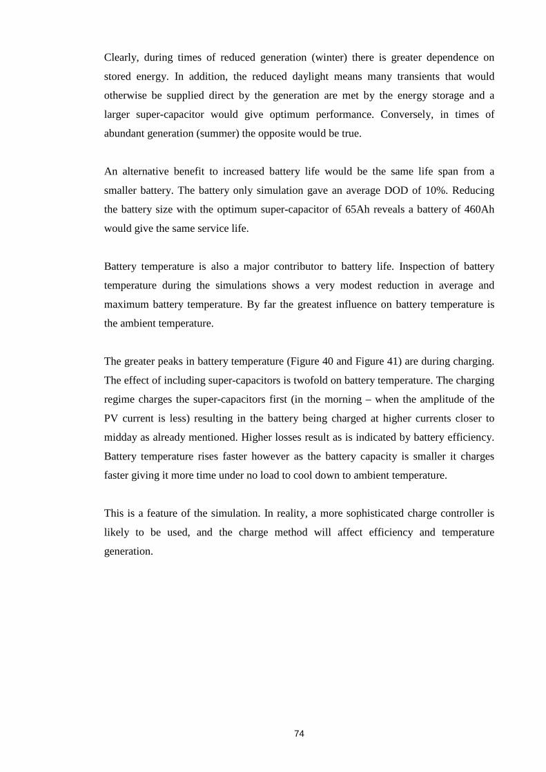
74

Clearly, during times of reduced generation (winter) there is greater dependence on

stored energy. In addition, the reduced daylight means many transients that would

otherwise be supplied direct by the generation are met by the energy storage and a

larger super-capacitor would give optimum performance. Conversely, in times of

abundant generation (summer) the opposite would be true.

An alternative benefit to increased battery life would be the same life span from a

smaller battery. The battery only simulation gave an average DOD of 10%. Reducing

the battery size with the optimum super-capacitor of 65Ah reveals a battery of 460Ah

would give the same service life.

Battery temperature is also a major contributor to battery life. Inspection of battery

temperature during the simulations shows a very modest reduction in average and

maximum battery temperature. By far the greatest influence on battery temperature is

the ambient temperature.

The greater peaks in battery temperature (Figure 40 and Figure 41) are during charging.

The effect of including super-capacitors is twofold on battery temperature. The charging

regime charges the super-capacitors first (in the morning – when the amplitude of the

PV current is less) resulting in the battery being charged at higher currents closer to

midday as already mentioned. Higher losses result as is indicated by battery efficiency.

Battery temperature rises faster however as the battery capacity is smaller it charges

faster giving it more time under no load to cool down to ambient temperature.

This is a feature of the simulation. In reality, a more sophisticated charge controller is

likely to be used, and the charge method will affect efficiency and temperature

generation.

75

10.3 The Solution

Enquiries were made to the Australian distributor of Maxwell BOOSTCAP ultra-

capacitors (see appendix). The 94F, 75V module retails for AU$3500 while the 165F,

48V module retails for AU$2500.

In all simulations the super-capacitor was discharged to 25% SOC. This equates to a

voltage range of 50%. I.e. operating a super-capacitor through 50% of its voltage range

delivers 75% of its energy.

The energy delivered by a capacitor (ΔE) is the difference between the total energy

available in the capacitor when fully charged and the energy remaining at the end of

discharge. Combining Equation 9 and Equation 13:

( )22

21

tot

2

remaintot VV2Eq

21 EEE(J) −××=−=∆ Equation 40

Recognising that 75% of the available energy is discharged due to the operational

voltage range of the DC/DC converter used with the super-capacitors (and assuming no

losses):

totE43 E(J) =∆ Equation 41

( )

( )

( )

000J 616 5E

24483

min60sec

h60min65Ah

E

VV3

qE

VV2Eq

21 E

43

tot

22

2

tot

22

21

22

tot

22

21

tot

2

tot

=

−×

××

=

−×=

−××=∴

Equation 42

76

Now from Equation 13:

F 9750C

000 616 52min

60sech

60min65Ah C

2Eq C

2

tot

2

=

×

××

=

=

Equation 43

Choosing the 48 volt 165 Farad unit and re-arranging Equation 12, recognising there is

1 super-capacitor in series:

09.59 Parallel#

1659750 Parallel#

C Series#C

Parallel#

Series#Parallel#CC

cell

eq

celleq

=

=

×=

×=

Equation 44

Say 59 units at AU$2500 per unit is AU$147 500, clearly not a financially viable option

given the monitored RAPS system cost less than $100 000 when new.

Consider also these units are 13.5kg [19]. 59 units would weigh 0.8 tonnes. The existing

8 batteries weigh 133kg per unit [7], total weight 1.063 tonnes. Adding 65Ah of super-

capacitor energy storage will result in a combined mass in the order of 1.8 tonnes.

For comparison consider the 75 volt unit. Assume again the DC/DC converter operates

through half the voltage range, i.e. 75 – 37.5 volts without losses.

77

From Equation 42:

( )

( )

000J 775 8E

5.37753

min60sec

h60min65Ah

E

VV3

qE

tot

22

2

tot

22

21

22

tot

=

−×

××

=

−×=

Equation 45

Again from Equation 13:

F 120 3C

000 577 82min

60sech

60min65Ah C

2Eq C

2

tot

2

=

×

××

=

=

Equation 46

Again re-arranging Equation 12 and recognising there is 1 super-capacitor in series:

19.33 Parallel#

943120 Parallel#

C Series#C

Parallel#

Series#Parallel#CC

cell

eq

celleq

=

=

×=

×=

Equation 47

Say 33 units at AU$3500 per unit is AU$115 500, also not a financially viable option.

These units are 25kg [19]. 33 units would weigh 0.825 tonnes, again resulting in an

energy storage mass of around 1.8 tonnes.

78

For comparison batteries similar to the Magnum 875 used in the monitored RAPS

system are available online for AU$1450.00 [25]. Eight such batteries would therefore

cost AU$11 600, less than 8% of the cost of the super-capacitor which will displace less

than 8% of the battery capacity.

Consider also the space required for storage. The existing battery bank of eight batteries

takes up 0.47m3 [7]. The 48 volt super-capacitor option would be an additional 0.6m3

[23] while the 75 volt option would be an additional 0.8m3 [24]. Both options are likely

to double the required space for storage.

For a typical land based RAPS system, an increase in size and mass of several orders of

magnitude is not likely to pose an insurmountable problem. Economic viability will be

the determining factor, and clearly the price of super-capacitors will prevent their use in

the near future. Additional costs such as DC/DC converters have not been considered

and there is little reason to, given the high cost of super-capacitors.

In reality, the battery is sized to the system and then selected from the supplier’s

available range. It is unlikely that a battery 8% smaller in capacity will be available to

match a super-capacitor.

The addition of a super-capacitor to a battery bank will therefore need to offer tangible

gains to the system at a reasonable cost. Consider the improvement in battery

performance from the simulation where battery life increased from 3387 cycles to 3577

cycles.

In today’s dollars, the battery-only cost:

cycleper 42.3$cycles 3387

11600$= Equation 48

At the same cost per cycle, the improvement in lifetime gives:

250 $12 cycleper $3.42 cycles 3577 =× Equation 49

79

It would be reasonable to expect someone to pay up to $12 250 for the increase in

performance. That is a difference of:

650$11600$12250$ =− Equation 50

Of course this over simplifies things, however a cost of $650 for 65Ah of super-

capacitor would make it a financially viable option. This means they would need to be

in the order of two hundred times cheaper. Put aside $1000 for a DC/DC converter and

there is no financial justification for the system at all.

For a reduction in battery size the benefits are greater. A 450Ah battery is available

online for AU$1010.00 [27]. Eight such batteries would therefore cost AU$8 080, this

represents a saving of AU$3520.00 on the 875Ah batteries. The inference from the

previous example is that if the price of a 65Ah super-capacitor bank was less than

$3520 users would consider them. This represents a reduction in price in the order of 40

times (excluding the cost of DC/DC converters and other costs incurred to integrate the

system).

As a measure of comparison, a 70Ah car battery costs $240 delivered and fitted by

Marshal Batteries [26]. Now four would be required to operate at 48V (approximately

$1000), or like the super-capacitors a DC/DC converter would be required but this

highlights the affordability of lead-acid batteries and therefore their dominance in the

market for energy storage.

80

11. Conclusion It was proposed that super-capacitors and lead-acid batteries would complement each

other as a hybrid energy store for RAPS systems. The initial assumption was that the

load would be characterised by a relatively constant base load suited to batteries and

transient spikes in load suited to super-capacitors.

This assumption was confirmed by monitoring a RAPS system in Boyup Brook and

analysing the data. The data collected from the RAPS system was then used as an input

to a simulated RAPS system with a hybrid super-capacitor lead-acid battery store.

Simulations were run with operating conditions of solar only generation with equal

hours of daylight and darkness and ambient temperature fixed at 25°C. There was

therefore 12 hours of generation starting at zero and peaking at an AC equivalent of 10

amps before reducing to zero.

A battery only case, consisting of 875Ah capacity was run followed by cases with

increasing super-capacitor capacity and diminishing battery capacity with the combined

capacity constant at 875Ah. The battery was dispatched to supply the base load while

the super-capacitor supplied the transient spikes in load. When charging the super-

capacitor was charged first and then the battery.

The optimum super-capacitor size was determined as 65Ah. This arrangement reduced

average battery DOD by 4.3% and therefore increased battery life from 9 years and 14

weeks to 9 years and 41 weeks, an improvement of 27 weeks or 5.6%. PV output was

reduced by 7.7% and net battery current reduced by 49%.

Based on the improvement in battery life and current battery costs, an estimate of super-

capacitor cost for the best case improvement in battery life is $650. The current cost of

super-capacitors is in the order of 200 times this amount.

Including a super-capacitor and reducing the size of the battery to one that will give the

same service life as the battery only case is financially more attractive. With a reduction

in battery size to 450Ah the saving is $3520. Super-capacitors would need to be forty

81

times cheaper to make this an economically attractive option. By comparison a similar

sized battery can be purchased for less than$1000, or 28% of this critical cost.

Implementing a super-capacitor less than 10% the size of the existing energy storage

can reduce battery size by around 50% and maintain the same performance. The cost of

super-capacitors is however prohibitive. The price would need to drop in the order of

forty times to compete with batteries.

82

12. Future Work Super-capacitors are sensitive to both heat and operating voltage. The model does not

represent voltage at all however temperature generation within the super-capacitors

could be implemented in the same manner as the batteries to see if there are detrimental

effects or if, like batteries, ambient temperature dominates and operation has little

influence over super-capacitor temperature. This would also allow super-capacitor

efficiency to be considered.

No other system efficiencies have been considered. Devices such as a DC/DC converter

and the existing inverter are likely to have efficiencies in the high 90% range that could

be included.

The charge regime implemented in this simulation was to simply “dump” all available

generation into the battery. A realistic charge controller implementing one of the charge

methods outlined would have a different affect on temperature and losses.

Scenarios of minimum and maximum generation could be investigated, particularly

intermittent solar generation that is likely to be experienced in cloudy conditions. This

potentially represents spikes in load caused by generation dropping off that could be

supplied by super-capacitors. Simulations could also incorporate the diesel generator

which would allow comparisons on costs associated with run-time (fuel and

maintenance).

A detailed control and dispatch system would need to be developed to implement super-

capacitors. A system incorporating a DC/DC converter and car battery in place of the

super-capacitor could be created at minimal expense (compared to super-capacitors) to

explore the “real world” issues that would be encountered in developing a hybrid

system, and gain some insight into the actual gains that might be made.

83

13. References [1] H.A. Kiehne. Ed., Battery Technology Handbook, 2nd ed New York: Marcel Dekker, 2003 [2] D.A.J. Rand, P.T. Moseley, J.Garche, C.D. Parker, Eds Valve-Regulated Lead-Acid Batteries Amsterdam: Elsevier, 2004 [E-book]. Available: Engineering Village. [3] R.M. Dell and D.A.J. Rand, Understanding Batteries, Cambridge: Royal Society of Chemistry, 2001 [4] N.K. Medora,A. Kusko. An Enhanced Dynamic Battery Model of Lead Acid Batteries Using Manufacturers’ Data 28th Annual International Telecommunications Energy Conference. September 2006. [5] D. Baert, A. Vervaet Lead-acid battery model for the derivation of Peukert’s law Electrochimica Acta, Volume 44, Issue 20, Pages 3491-3504, June 1999 [online] Available: ScienceDirect, http://www.sciencedirect.com/ [Accessed October 30, 2010] [6] Smart Gauge Electronics Peukert and Charging [online] Available: http://www.smartgauge.co.uk/peukert_chg.html [Accessed October 17, 2010] [7] Magnum Premium Deep Cycle Batteries. Product Specification. Supplied by WA Solar Supplies September 13 2010 [8] Anders, A. Tracking down the origin of arc plasma science I. Early pulsed and oscillating discharges IEEE Transactions on Plasma Science, Volume: 31, Issue: 5, Part: 2 2003 [9] P. Sharma, T. S. Bhatti. A review on electrochemical double layer capacitors Energy Conversion and Management Volume: 51, Issue: 12, December 2010 [10] R. L. Spyker, R. M. Nelms. Optimization of Double Layer Capacitor Arrays. IEEE Transactions on Industry Applications Volume: 36, Number: 1, January/Febuary 2000 [11] A. R. Hambley. Electrical Engineering Principles and Applications New Jersey, Prentice Hall 2008 [12] A. Helwig, T. Ahfock. Ultra-capacitor Assisted Battery Storage for Remote Area Power Supplies: A Case Study, Adelaide, Australasian Universities, Power Engineering Conference 2009, AUPEC 2009, September 2009 [13] Application Note How to Determine the Appropriate Size Ultracapacitor for Your Application. Maxwell Technologies, Document 1007236, Rev 2 [online] Available: http://www.maxwell.com/pdf/uc/General_Sizing-1007236.pdf [accessed October 17, 2010] [14] Product Guide BOOSTCAP Ultracapacitors Maxwell Technologies, [online] Available: http://www.maxwell.com/pdf/1014627_BOOSTCAP_Product_Guide.pdf [accessed October 31, 2010]

84

[15] Application Note BOOSTCAP Energy Storage Modules Life Duration Estimation. Maxwell Technologies, [online] Available: http://www.maxwell.com/pdf/uc/application-notes/ApplicationNote1012839_1.pdf [accessed October 17, 2010] [16] R. Kotz, M. Hahn, R. Gally. Temperature behavior and impedance fundamentals of supercapacitors Journal of Power Sources, Volume 154, Issue 2, 21 March 2006 [online] Available: Engineering Village. [accessed October 17, 2010]

[17] Battery and Energy Technologies. Battery Performance Characteristics Electropaedia. [online] Available: http://www.mpoweruk.com/performance.htm#ragone [accessed October 17, 2010] [18] M.E. Glavin, P.K.W. Chan, S. Armstrong, W.G. Hurley. Stand-alone Photovoltaic Supercapacitor Battery Hybrid Energy Storage System 13th Power Electronics and Motion Control Conference, September 2008. [19] Data Sheet BOOSTCAP Ultracapacitors Product Comparison. Maxwell Technologies, [online] Available: http://www.maxwell.com/pdf/uc/Maxwell_UC_comparison.pdf [accessed October 17, 2010] [20] Handbook for Stationary Lead-Acid Batteries Part 1. Basics, Design, Operation Modes and Applications, 3rd ed, Berlin, EXIDE Technologies 2008 [online] Available: http://www.elektrotec-berlin.de/download/eng/Handbook,%20part%201,%20edition%203.pdf [Accessed September 26, 2010] [21] B. Wichert. Control of Photovoltaic-Diesel Hybrid Energy Systems, Appendix C, PV-Diesel Hybrid Energy Simulation PhD Dissertation, Curtin University, 2000 [22] C. M. Close, D. K. Frederick, J. C. Newell. Modeling and Analysis of Dynamic Systems, 3rd ed, New York, John Wiley and Sons, 2002. [23] Data Sheet 48 Volt Modules BMOD0083 P048, BMOD0110 P048, BMOD0165 P048, Maxwell Technologies, [online] Available: http://www.maxwell.com/ultracapacitors/datasheets/DATASHEET_48V_series_1009365.pdf [Accessed November 08, 2010] [24] Data Sheet 75 Volt Module BMOD0094 P075 B02, Maxwell Technologies, [online] Available: http://www.maxwell.com/ultracapacitors/datasheets/DATASHEET_BMOD0094_1012179.pdf [Accessed November 08, 2010] [25] Enersun SSR Tubular Positive Flooded Cell 875Ah Century Yuasa 6V Deep Cycle Battery $1450.00 Solar Online Australia [online] Available: http://www.solaronline.com.au/875ah-century-yuasa-6v-deep-cycle-battery.html [Accessed November 08, 2010]

85

[26] Exide Extreme N70EXL Battery $240 Marshal online. [online] Available: http://www.marshallbatteries.com.au/fitment-results.php [Accessed November 08, 2010] [27] Enersun SSR Tubular Positive Flooded Cell 450Ah Century Yuasa 6V Deep Cycle Battery $1010.00 Solar Online Australia [online] Available: http://www.solaronline.com.au/450ah-century-yuasa-6v-deep-cycle-battery.html [Accessed November 08, 2010]

86

14. Appendix Price for super-capacitors. "dsarelius" <dean@glyn.com.au>

04/11/2010 10:41 AM

To "'Bruce Blechynden'" <bruce.blechynden@horizonpower.com.au> cc

Subject RE: Boostcap Ultra capacitors

Dear Bruce, Thank you for your email. We do not presently have these modules available from stock but can arrange to have them shipped within 4-6 weeks ex Maxwell. http://www.maxwell.com/ultracapacitors/products/modules/bmod0094-75v.asp Part No: BMOD0094 P075 Description: 94F, 75V module Qty/Price 1pcs AU$3500 Delivery: 4-6 wks aro http://www.maxwell.com/ultracapacitors/products/modules/bmod0083-48-6v.asp Part No: BMOD0165 P048 Description: 165F, 48V module Qty/Price 1pcs AU$2500 Delivery: 4-6 wks aro P&H: TNT Road - WA (6102) AU$45.00 for one module..! Regards, Dean Sarelius Australian Sales Manager Glyn Ltd Suite 7/201 29-31 Solent Circuit Baulkham Hills NSW Australia 2153 Ph: +61 2 8850 0320 M: 0437 877 001

87

Catalogue of appliance use on monitored RAPS system.

Date Time Appliance

03/09/2010 3:50PM Boot up computer

03/09/2010 3:52PM Kettle

03/09/2010 5:53PM Microwave

04/09/2010 6:58AM Kettle

04/09/2010 8:59AM Toaster

04/09/2010 9:14AM Bread Maker

05/09/2010 9:25AM Arc welder

06/09/2010 1:00PM Ironing

07/09/2010 6:38PM Sandwich maker

08/09/2010 8:59AM Microwave

10/09/2010 8:15AM Washing machine

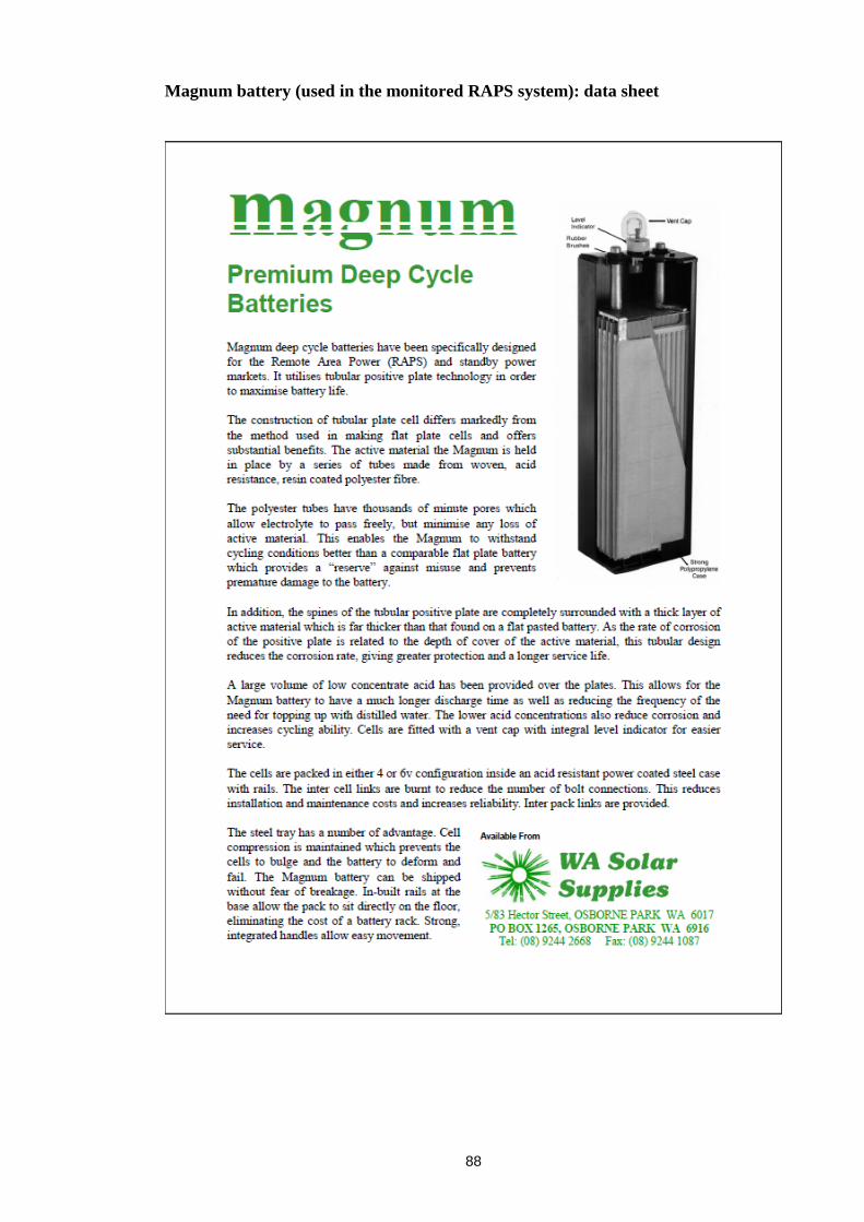
88

Magnum battery (used in the monitored RAPS system): data sheet

89

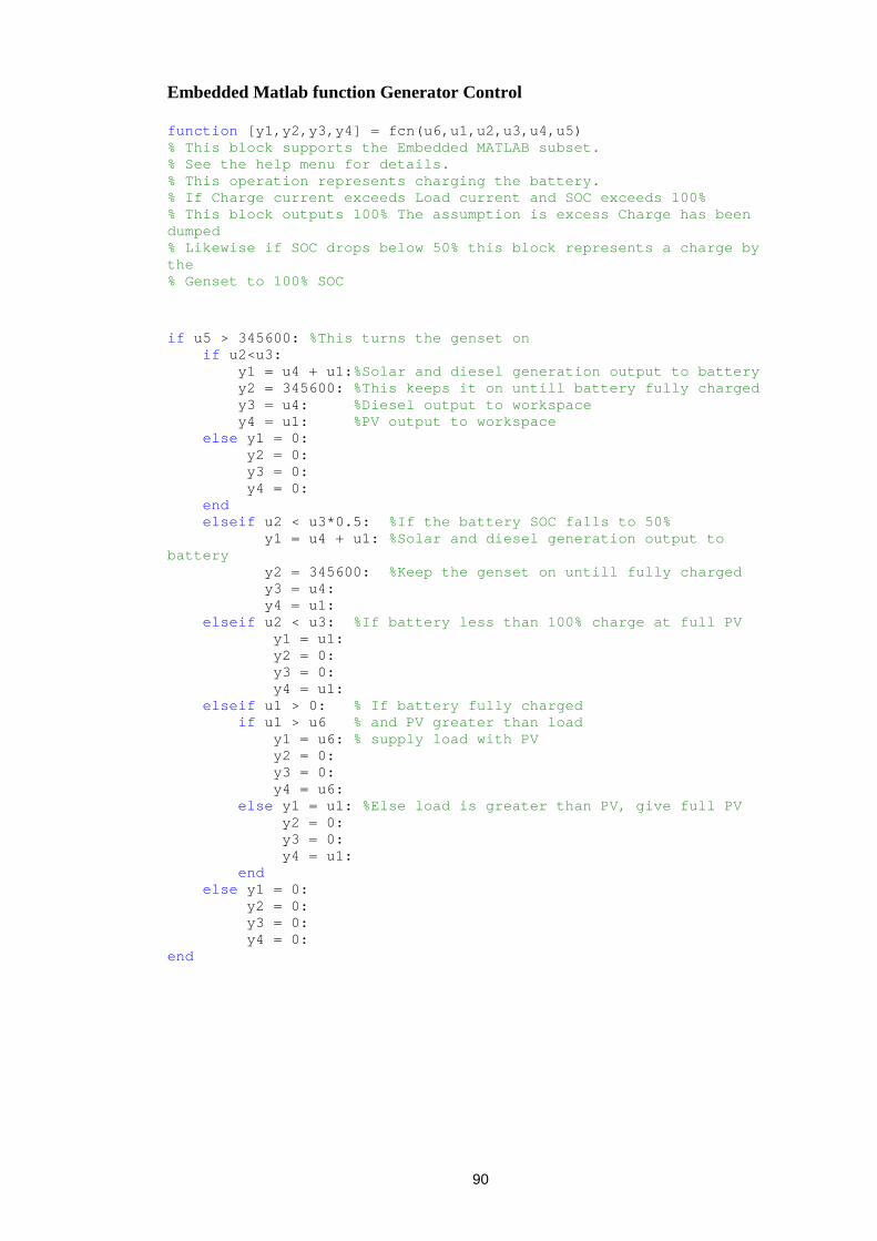
90

Embedded Matlab function Generator Control function [y1,y2,y3,y4] = fcn(u6,u1,u2,u3,u4,u5) % This block supports the Embedded MATLAB subset. % See the help menu for details. % This operation represents charging the battery. % If Charge current exceeds Load current and SOC exceeds 100% % This block outputs 100% The assumption is excess Charge has been dumped % Likewise if SOC drops below 50% this block represents a charge by the % Genset to 100% SOC if u5 > 345600: %This turns the genset on if u2<u3: y1 = u4 + u1:%Solar and diesel generation output to battery y2 = 345600: %This keeps it on untill battery fully charged y3 = u4: %Diesel output to workspace y4 = u1: %PV output to workspace else y1 = 0: y2 = 0: y3 = 0: y4 = 0: end elseif u2 < u3*0.5: %If the battery SOC falls to 50% y1 = u4 + u1: %Solar and diesel generation output to battery y2 = 345600: %Keep the genset on untill fully charged y3 = u4: y4 = u1: elseif u2 < u3: %If battery less than 100% charge at full PV y1 = u1: y2 = 0: y3 = 0: y4 = u1: elseif u1 > 0: % If battery fully charged if u1 > u6 % and PV greater than load y1 = u6: % supply load with PV y2 = 0: y3 = 0: y4 = u6: else y1 = u1: %Else load is greater than PV, give full PV y2 = 0: y3 = 0: y4 = u1: end else y1 = 0: y2 = 0: y3 = 0: y4 = 0: end

91

Embedded Matlab function Capacitor Control function [y2,y1] = fcn(u3,u1,u2) % This block supports the Embedded MATLAB subset. % See the help menu for details. % This operation represents charging the battery. % If Charge current exceeds Load current and SOC exceeds 100% % This block outputs 100% The assumption is excess Charge has been dumped % Likewise if SOC drops below 50% this block represents a charge by the % Genset to 100% SOC if u1 < -(u3 + 1) %Step in load 1 amp more than base load (battery current is -ve) if u2 > 0.25 %and cap SOC greater than 25% y1 = -u1 - u3: %add step to batt (u1 is -ve when batt discharging) y2 = u1 + u3: %take step from cap i.e. supply load with capacitor else y1 = 0: y2 = 0: end elseif u2 <= 1: %Cap not charged if u1 > 0 %batt charging (+ve current) y1 = -u1: %charge capacitor to 100% first (battery gets nothing yet) y2 = u1: %add current to cap else y1 = 0: %Cap not charged and bat discharging (no PV) y2 = 0: %To charge cap slowly from batt set y1=-y2<0, (say 1 amp) end else y1 = 0: y2 = 0: end Embedded Matlab function within Load Profile calling load data function y = fcn(u8,u1,u2,u3,u4,u5,u6,u7) % This block supports the Embedded MATLAB subset. % See the help menu for details. if u8 <=86400 y = u1: elseif u8 <=86400*2 y = u2: elseif u8 <=86400*3 y = u3: elseif u8 <=86400*4 y = u4: elseif u8 <=86400*5 y = u5: elseif u8 <=86400*6 y = u6: else y = u7: end