Super- and sub-rotating equatorial jets in shallow … and sub-rotating equatorial jets in shallow...

Under consideration for publication in J. Fluid Mech. 1

Super- and sub-rotating equatorial jets in shallow water modelsof Jovian atmospheres: Newtonian cooling versus Rayleigh

friction

Emma S. Warneford and Paul J. Dellar†OCIAM, Mathematical Institute, University of Oxford, Andrew Wiles Building, Radcliffe Observatory Quarter, Woodstock Road,

Oxford, OX2 6GG, UK

(Received 27 August 2013, in revised form 22 January 2014, 28 June 2014, 31 March 2015, 30 December 2016)

Numerical simulations of the shallow water equations on rotating spheres produce mixtures of robust vortices andalternating zonal jets, as seen in the atmospheres of the gas giant planets. However, simulations that include Rayleighfriction invariably produce a sub-rotating (retrograde) equatorial jet for Jovian parameter regimes, whilst observations ofJupiter show a super-rotating (prograde) equatorial jet that has persisted over several decades. Super-rotating equatorialjets have recently been obtained in shallow water simulations that include a Newtonian relaxation of perturbations to thelayer thickness to model radiative cooling to space, and in simulations of the thermal shallow water equations that includea similar relaxation term in their temperature equation. Simulations of global quasigeostrophic forms of these differentmodels produce equatorial jets in the same directions as the parent models, suggesting that mechanism responsible forsetting the direction lies within quasigeostrophic theory. We provide such a mechanism by calculating the effective forceacting on the thickness-weighted zonal mean flow due to the decay of an equatorially trapped Rossby wave. Decay due toNewtonian cooling creates an eastward zonal mean flow at the equator, consistent with the formation of a super-rotatingequatorial jet, while decay due to Rayleigh friction leads to a westward zonal mean flow at the equator, consistent withthe formation of a sub-rotating equatorial jet. In both cases the meridionally integrated zonal mean of the absolute zonalmomentum is westward, consistent with the standard result that Rossby waves carry westward pseudomomentum, butthis does not preclude the zonal mean flow being eastward on and close to the equator.

1. IntroductionObservations of Jupiter’s atmosphere reveal a highly turbulent cloud deck containing long-lived coherent vortices

such as the Great Red Spot that are transported around the planet by an alternating pattern of zonal jets (Vasavada &Showman 2005). Following the pioneering non-divergent barotropic model of Williams (1978), shallow water theoryhas been widely used to model the Jovian atmosphere (Cho & Polvani 1996a,b; Dowling & Ingersoll 1989; Iacono et al.1999a,b; Ingersoll 1990; Marcus 1988; Scott & Polvani 2007, 2008; Showman 2007; Williams & Yamagata 1984). Thevisible cloud deck is treated as a homogeneousm dynamically active layer separated from a much deeper and relativelyquiescent lower layer by a sharp density contrast, which may be linked to latent heat being released at the water vapourcondensation level. The equivalent barotropic approximation (Dowling & Ingersoll 1989; Gill 1982) gives a closed setof shallow water equations for the flow in the cloud deck.

Numerical simulations of the shallow water equations on rotating spheres with Jovian parameter values reproducea mixture of robust vortices and alternating zonal jets. The latter arise naturally from the nonlinear inverse cascadecharacteristic of two-dimensional turbulence being arrested through coupling to Rossby waves at the Rhines (1975)scale, though the quasilinear “zonostrophic instability” mechanism may also have a role (Srinivasan & Young 2012,2014, and references therein). The equatorial jets are invariably sub-rotating (retrograde) in both freely decaying andforced-dissipative simulations in the Jovian regime (e.g. Cho & Polvani 1996a,b; Iacono et al. 1999a,b; Scott & Polvani2007; Showman 2007). By contrast, the mean zonal wind profiles in figure 1, as obtained from tracking visible featuresin Jupiter’s atmosphere, show a broad, super-rotating equatorial jet. The similarity of the two profiles, taken from theVoyager 2 (Limaye 1986) and Cassini (Porco et al. 2003) missions over 20 years apart, demonstrates the remarkablestability of Jupiter’s zonal winds, and the longevity of the super-rotating equatorial jet.

Forced-dissipative shallow water simulations typically include a Rayleigh friction term to absorb the slow inversecascade of energy past the Rhines scale to the largest scales in the system, which tends to create large coherent vorticesin place of the alternating zonal jets (e.g. Vasavada & Showman 2005). Scott & Polvani (2007, 2008) added an additional

† Email address for correspondence: [email protected]

arX

iv:1

401.

6406

v2 [

phys

ics.

flu-

dyn]

4 J

an 2

017

2 E. S. Warneford and P. J. Dellar

−100 0 100 200

−80

−60

−40

−20

0

20

40

60

80

Mean Zonal Wind (m s−1

)

Pla

neto

gra

ph

ic L

atitu

de (

deg

rees)

Voyager

Cassini

FIGURE 1. Mean zonal wind profiles for Jupiter. The red solid line shows Voyager 2 data from Limaye (1986) and the blue dashedline shows Cassini data from Porco et al. (2003).

radiative relaxation term with timescale τrad to the continuity equation in their shallow water model:

ht +∇ · (hu) = − (h− h0) /τrad, (1.1a)ut + (u · ∇)u+ f z × u = −g′∇h+ F − u/τfric, (1.1b)

Here h is the thickness of the active layer, commonly called “height”, u is the depth-averaged horizontal velocity,f = 2Ω sinφ is the Coriolis parameter at latitude φ on a planet rotating with angular velocity Ω, ∇ is the horizontalgradient operator, z is a unit vector in the local vertical direction, F is an isotropic random forcing, and τfric is thetimescale for Rayleigh friction. The reduced gravity is g′ = g∆ρ/ρ0, where g is the actual gravitational acceleration,∆ρ is the density contrast between the cloud deck and the lower layer, and ρ0 is a reference density. These parametersare possibly constrained by observations of what appear to be internal gravity waves radiating from the impact pointsof Shoemaker–Levy comet debris (Dowling 1995; Ingersoll et al. 2007), although this interpretation is not without itscritics (Walterscheid et al. 2000).

The right hand side of (1.1a) models the effects of radiation to space with a Newtonian relaxation of h towards itsconstant mean value h0 on the time scale τrad, following earlier shallow water models of the upper ocean mixed layer(Hirst 1986; Philander et al. 1984) and the terrestrial stratosphere (Juckes 1989; Polvani et al. 1995; Thuburn & Lagneau1999). Scott & Polvani’s (2007; 2008) simulations of this system with dissipation only by thickness relaxation (no τfricterm) produced a sharply localised super-rotating equatorial jet, as do our subsequent simulations described in §3, andin Warneford & Dellar (2014).

Thermal shallow water theory introduced by Lavoie (1972) to describe atmospheric mixed layers over frozen lakes.It permits horizontal variations of the thermodynamic properties of the fluid within each layer, which are taken to beuniform in the standard shallow water equations. The density contrast ∆ρ thus becomes a dynamical variable. However,subsequent developments of thermal shallow water theory have been much more focused on modelling the oceanicmixed layer (Hirst 1986; McCreary et al. 1991; McCreary & Kundu 1988; McCreary & Yu 1992; Ripa 1993, 1995,1996a,b; Røed & Shi 1999; Schopf & Cane 1983).

Warneford & Dellar (2014) simulated Jovian atmospheres using the thermal shallow water equations

ht +∇ · (hu) = 0, (1.2a)Θt + (u · ∇) Θ = − (Θh/h0 −Θ0) /τrad, (1.2b)

ut + (u · ∇)u+ f z × u = −h−1∇(12Θh2

)+ F − u/τfric. (1.2c)

We introduce the symbol Θ = g∆ρ/ρ0 for the reduced gravity to emphasise that it is now a function of space and time.The first term on the right hand side of (1.2c) is then the usual shallow water pressure gradient term, as rewritten fora spatially varying reduced gravity. The right hand side of (1.2b) is a Newtonian cooling term that represents radiativerelaxation towards a temperature Θ0h0/hwith time scale τrad. We show below that this form of coupling between Θ andh changes the behaviour of equatorially trapped Rossby waves in almost exactly the same way as the radiative relaxationof h itself in Scott & Polvani’s (2007; 2008) model. In particular, the damping rates calculated in §4 are very similarfunction of wavenumber and τrad. The resulting Reynold stresses calculated in §5 have very similar spatial structures

Super- and sub-rotating equatorial jets: Newtonian cooling versus Rayleigh friction 3

between the two models, and are proportional to the difference between the dimensionless radiative and frictional decayrate constants in both models.

The thermal shallow water equations (1.2a,b,c) conserve both mass and momentum in the absence of the τfric andF terms, unlike the Scott and Polvani model (1.1a,b). Simulations of the thermal shallow water equations for Jovianparameter values (reported in §3 and Warneford & Dellar 2014) reproduce a super-rotating equatorial jet, and more sub-stantial mid-latitude jets than simulations of the Scott & Polvani (2007, 2008) model. Henceforth, for brevity we refer tothe radiative relaxation terms as relaxation and the Rayleigh friction term as friction. We also refer to equations (1.1a,b)as the “standard” shallow water equations to distinguish them from the thermal shallow water equations (1.2a,b,c).

Quasi-geostrophic (QG) theory (Charney 1949; Obukhov 1949) offers a simplified description of slow vortical mo-tions that filters out inertia-gravity waves. Although QG theory is usually employed for mid-latitude beta-planes, Mat-suno (1970, 1971) presented a global QG theory for fully stratified atmospheres on spheres. Verkley (2009) and Schubertet al. (2009) revived this theory for the standard shallow water equations on a sphere in the form

qt + [ψ, q] = 0, q = f +∇2ψ − L−2D ψ, (1.3)

where the Jacobian [ψ, q] = z · (∇ψ ×∇q). The Rossby deformation scale is LD = c/f , where c is the speed oflong surface gravity waves. Both f and LD vary with latitude when QG theory is used in spherical coordinates. The soleevolving variable is the potential vorticity q, which is advected by the velocity field derived from a streamfunction ψ. Theelliptic equation relating ψ to q involves the spatially varying Coriolis parameter f . It corresponds to Daley’s (1983)simplest form of geostrophic balance, as justified by assuming that ψ varies on lengthscales much smaller than theplanetary scales on which f varies. The system (1.3) reduces to the familiar beta-plane QG equations on approximatingf by f0 + βy in the first term, and by f0 in the second term. Warneford (2014) derived a thermal form of this global QGtheory, building on the beta-plane thermal QG equations in Ripa (1996a) and Warneford & Dellar (2013). Numericalsimulations produced super-rotating equatorial jets when the dimensionless radiative relaxation time τrad is sufficientlyshort, as did simulations of the corresponding global QG form of Scott & Polvani’s (2007; 2008) shallow water modelwith a relaxing thickness. By contrast, both QG models produced sub-rotating equatorial jets when τrad is sufficientlylong. The mechanism responsible for setting the equatorial jet direction must therefore lie within QG theory. This focusesattention on momentum fluxes due to Rossby waves, rather than by inertia-gravity waves, or the equatorially trappedKelvin and Yanai waves. None of these waves exist in QG theory.

2. Momentum transport by Rossby wavesDickinson (1969) showed that the meridional flux of zonal momentum due to Rossby waves produces a net eastward

acceleration in regions where Rossby waves are generated, and a net westward acceleration in regions where Rossbywaves are dissipated. This argument was further developed by Green (1970) and Thompson (1971). A detailed versionbased on ray theory may be found in Held (2000) and Vallis (2006). The QG equations on a mid-latitude beta planelead to the Rossby wave dispersion relation ω = −βk/(k2 + `2 +L2

D) for plane-wave disturbances with streamfunctionψ = ψ exp(i(kx+ `y − ωt)) implies a meridional group velocity

∂ω

∂`=

2βk`

(k2 + `2 + L2D)2

, (2.1)

while the off-diagonal component of the Reynolds stress (see §4 for notation) is

〈u′v′〉 = −1

2ψ2k`. (2.2)

The radiation condition requires the meridional group velocity to point away from wave sources, so the sign of k` issuch as to create a flux of westward (negative) zonal momentum away from sources of Rossby waves towards regionswhere Rossby waves are dissipated.

For example, Schneider & Liu (2009) and Liu & Schneider (2010) identified Rossby wave sources due to divergentmotions associated with the breakdown of geostrophy near the equator in their three-dimensional simulations of Jovianatmospheres. Propagation of these Rossby waves to higher latitudes thus creates a net eastward acceleration at theequator according to the above theory, which is consistent with the formation of super-rotating equatorial jets in theirsimulations.

However, the focus of our present paper will be on the equatorially trapped Rossby waves that play a key role in near-equatorial dynamics (e.g. Gill 1982; Khouider et al. 2013; Majda & Klein 2003; Matsuno 1966; McCreary 1985). Thesewaves are confined by a Gaussian envelope whose extent scales with the equatorial deformation scale Leq =

√c/(2β).

This corresponds to latitudes within about 30 of the equator for Jovian parameters (see §4). We therefore need to


compute the latitude-dependence of the momentum fluxes inside the scale of this envelope, for which a ray theoryapproach is inadequate.

The generalised Lagrangian mean (GLM) theory is a powerful approach for addressing this and other problems inwave-mean flow interaction (Andrews & McIntyre 1976a; Buhler 2000, 2014). It defines the Lagrangian mean of anarbitrary field φ(x, t) by

φL(x, t) = φ(x+ ξ(x, t), t), (2.3)

where (· · · ) is some linear averaging operator, and ξ(x, t) is a Lagrangian displacement field such that x + ξ(x, t) isthe actual position of the particle whose mean position is x at time t. GLM theory establishes circumstances for thevalidity of a “pseudomomentum rule” (Buhler 2000, 2014; McIntyre 1981) under which the waves behave for somepurposes as if they carried a momentum equal to their pseudomomentum and the background fluid were absent. Thepseudomomentum is a disturbance quantity related to the pseudoenergy defined in §5.

A linearized version of GLM for small ξ was presented in Andrews & McIntyre (1976a, 1978). However, the La-grangian picture of a fluid evolving through displacements of indestructible particles fits awkwardly with the mass sourceor sink term on the right hand side of (1.1a) that models radiative relaxation. In particular, lack of mass conservationrequires modification of Buhler’s (2000) shallow water pseudomomentum rule obtained from GLM theory. Neverthe-less, McIntyre (2014, personal communication) has established, firstly, that is possible to reproduce our results belowusing the linearised GLM theory slightly adapted to apply to (1.1a,b) and, secondly, that an eastward zonal accelerationat the equator is obtained for two interesting cases, (1) equatorially trapped Rossby waves freely decaying by radiativerelaxation – as we compute independently below – and (2) the same waves, but maintained at constant amplitude by abalance between forcing and dissipation, with the dissipation again by radiative relaxation but with the forcing mimickedby negative Rayleigh friction. The linearised GLM theory shows why negative Rayleigh friction, if spatially uniform,has an effect qualitatively similar to that of free temporal decay – as illustrated by the curves in figure 4b of Andrews &McIntyre (1976a) with suitable sign changes.

Following the approach of McIntyre & Norton (1990) for stratified fluids, Buhler (2000) formulated a general ap-proach for shallow water equations of the form

ht +∇ · (hu) = 0, (2.4a)ut + (u · ∇)u+ f z × u = −g′∇h+ F (2.4b)

with a general term F, not necessarily a forcing. The shallow water potential vorticity q = (f + ζ)/h, where ζ =z · (∇× u) is the relative vorticity, evolves according to

∂t(hq) +∇ · (hqu− F⊥) = 0, (2.5)

with an extra flux F⊥ = z × F . Buhler’s (2000) pseudomomentum rule holds for systems of this form that conservelinear momentum, those for which hF = ∇ · σ is the divergence of a stress tensor σ

However, neither of of the shallow water models from §1 fits this form. The shallow water system with relaxation ofthe thickness does not conserve momentum. In the absence of forcing and friction, (1.1a) and (1.1b) together imply

(hu)t +∇ ·(huu+ 1

2g′h2I

)+ f z × (hu) = − (h− h0)u/τrad, (2.6)

where I is the 2× 2 identity matrix. Moreoever, the potential vorticity for the system (1.1a,b) obeys

(hq)t +∇ · (hqu+ u⊥/τfric) = 0, (2.7)

where u⊥ = z × u, while the potential vorticity in the thermal shallow water equations (1.2a–c) obeys

(hq)t +∇ · (hqu− 12h∇

⊥θ + u⊥/τfric) = 0. (2.8)

Radiative relaxation thus does not contribute to either potential vorticity equation. However, (2.8) contains an extra terminvolving the perpendicular temperature gradient∇⊥θ = z ×∇θ that arises from the curl of the (1/2)h∇Θ term onthe right hand side of (1.2c). The thermal shallow water equations thus do not materially conserve potential vorticity,even in the absence of forcing and dissipation. Instead, the total potential vorticity inside a closed isotherm is conserved.This is the thermal shallow water analogue of the potential vorticity impermeability property of isentropic surfaces inthree-dimensional stratified fluids (Haynes & McIntyre 1990).

Since the Scott & Polvani (2007, 2008) radiatively relaxed shallow water model lacks both mass and momentumconservation, and hence does not fit naturally into the above general frameworks, in §4 and §5 below we derive fromfirst principles equations for the evolution of the thickness-weighted zonal mean velocity components 〈u〉∗ and 〈v〉∗(see §5 for notation) caused by the decay of an equatorially trapped Rossby wave by friction and/or radiative relaxation.


a 2π/Ω√g′h0 g τrad τfric

7.1× 107m 9.9 hours 678 m s−1 26 m s−2 429 hours 9900 hours

TABLE 1. Parameter values for Jupiter (from Beebe 1994; Ingersoll 1990; Warneford & Dellar 2014).

−180 −90 0 90 180N

EQ

S

EQ

N

Longitude (degrees)

Latitu

de

Bottom Planet

Top Planet

FIGURE 2. Schematic of the doubly-periodic Cartesian domain used for the numerical simulations. Each half of the domainrepresents a full planet, so for ease of interpretation we show simulation results for just the top planet.

3. Numerical experimentsWe now show some numerical simulations of the standard shallow water equations with dissipation only through

friction (i.e. (1.1a,b) with no τrad term), the Scott & Polvani (2007, 2008) model with relaxation of the thickness, andour thermal shallow water model. Table 1 gives typical Jovian values for the planetary radius a, angular velocity Ω,gravitational acceleration g, and internal wave speed

√g′h0. The last is deduced from impacts of Shoemaker–Levy

comet debris (Dowling 1995; Ingersoll et al. 2007), and implies that there are 232 polar deformation scales LD =√g′h0/(2Ω) around the circumference. Simulations with radiative relaxation used a timescale τrad of 43 Jovian days,

as calculated for a temperature of 120K at the 25 millibar pressure level, and all simulations employed a friction with atime scale of 1000 Jovian days. Liu & Schneider (2010) used the 25 millibar pressure level when comparing their three-dimensional simulations with observations of Neptune. Calculating τrad at the 25 millibar pressure level for both planetsleads to a super-rotating equatorial jet for Jupiter, and a sub-rotating equatorial jet for Neptune, in our thermal shallowwater model. The theory in §5 below suggests that the direction of the equatorial jet is insensitive to these parametersprovived the radiative relaxation timescale remains much shorter than the frictional timescale.

Simulations of geostrophic turbulence in the Jovian regime require thousands of rotation periods to reach statisticallysteady states. The superior memory bandwidth and peak floating point performance of graphical processing units (GPUs)thus becomes attractive, but existing spherical harmonic transform algorithms for GPUs only achieve performance paritywith conventional microprocessors (Hupca et al. 2012). We therefore employed the doubly-periodic Cartesian domainsketched in figure 2, which we refer to as the square planet domain. The horizontal axis denotes longitude, whilethe vertical axis denotes latitude. Starting from the north pole at the top of the domain and moving down, we reach theequator a quarter of the way down, and the south pole half way down. We then continue to reach the equator again, beforereturning to the north pole at the bottom of the domain. We imagine following a meridian (constant longitude line) fromthe north pole to the equator to the south pole, and then following a second meridian with longitude offset by 180 backacross the equator to the north pole. The Coriolis force is still fully varying in latitude and is defined in the simulationsby f(y) = 2Ω cos(2πy/ymax), where ymax is the length of the side of the square planet domain, i.e. the circumferenceof Jupiter (see table 1). The Coriolis force and all its derivatives are thus doubly periodic. This allowed us to exploit ahigh performance GPU fast Fourier transform library. We discretized the domain using 1024× 1024 Fourier collocationpoints, and used the Hou & Li (2007) spectral filter to control the build-up of enstrophy at the highest wavenumbers.We integrated the resulting large system of ordinary differential equations using the standard fourth-order Runge–Kuttascheme, with a time step determined dynamically from the Courant–Friedrichs–Lewy stability condition.

Our initial conditions were h = h0 and u = v = 0 for all runs, and Θ = Θ0 for the thermal shallow water simulation.Following Scott & Polvani (2007, 2008) we applied a divergence-free isotropic random forcing F that is localised to a


(a)

−180 −90 0 90 180 −90

−45

0

45

90

Longitude (degrees)

Latit

ude

(deg

rees

)

−4

−2

0

2

4

(b)

−180 −90 0 90 180 −90

−45

0

45

90

Longitude (degrees)

Latit

ude

(deg

rees

)

−4

−2

0

2

4

(c)

−180 −90 0 90 180 −90

−45

0

45

90

Longitude (degrees)

Latit

ude

(deg

rees

)

−4

−2

0

2

4

FIGURE 3. Absolute vorticity ωa = vx−uy +f(y) in units of 10−4 s−1 for (a) the standard shallow water equations with dissipationby friction alone, (b) the standard shallow water equations with friction and radiative relaxation of the thickness, and (c) the thermalshallow water equations with friction and radiative relaxation of the temperature.

narrow annulus of wavenumbers |k| ∈ [40, 44] in Fourier space, counting the longest sinusoidal mode in the domain aswavenumber 1. We forced each mode inside this annulus with amplitude εf using random phases that were δ-correlated(white) in time. This forcing is widely used in numerical studies of zonal jet formation, and models the energy injected bythree-dimensional convection at horizontal lengthscales comparable to the deformation radius. Our simulations slowlyadjusted the amplitude of the forcing εf to reach a prescribed value of the total kinetic energy in the eventual statisticalsteady state. Further details of the numerical models, parameters, and simulation outputs may be found in Warneford(2014) and Warneford & Dellar (2014).


(a)

−180 −90 0 90 180 −90

−45

0

45

90

Longitude (degrees)

Latit

ude

(deg

rees

)

−150

−100

−50

0

50

100

150

(b)

−180 −90 0 90 180 −90

−45

0

45

90

Longitude (degrees)

Latit

ude

(deg

rees

)

−150

−100

−50

0

50

100

150

(c)

−180 −90 0 90 180 −90

−45

0

45

90

Longitude (degrees)

Latit

ude

(deg

rees

)

−150

−100

−50

0

50

100

150

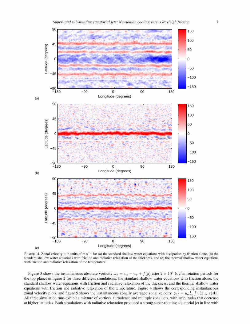
FIGURE 4. Zonal velocity u in units of m s−1 for (a) the standard shallow water equations with dissipation by friction alone, (b) thestandard shallow water equations with friction and radiative relaxation of the thickness, and (c) the thermal shallow water equationswith friction and radiative relaxation of the temperature.

Figure 3 shows the instantaneous absolute vorticity ωa = vx − uy + f(y) after 2 × 104 Jovian rotation periods forthe top planet in figure 2 for three different simulations: the standard shallow water equations with friction alone, thestandard shallow water equations with friction and radiative relaxation of the thickness, and the thermal shallow waterequations with friction and radiative relaxation of the temperature. Figure 4 shows the corresponding instantaneouszonal velocity plots, and figure 5 shows the instantaneous zonally averaged zonal velocity, 〈u〉 = y−1max

∫u(x, y, t) dx.

All three simulation runs exhibit a mixture of vortices, turbulence and multiple zonal jets, with amplitudes that decreaseat higher latitudes. Both simulations with radiative relaxation produced a strong super-rotating equatorial jet in line with


−100 −50 0 50 100 150−90

−60

−30

0

30

60

90

mean zonal wind (m s−1

)

latitu

de

(deg

ree

s)

friction only

thickness

thermal

FIGURE 5. Mean zonal velocity 〈u〉 against latitude for simulations of the standard shallow water equations with dissipation byfriction alone, the standard shallow water equations with friction and radiative relaxation of the thickness, and the thermal shallowwater equations with friction and radiative relaxation of the temperature

observations of Jupiter. However, our simulation of the standard shallow water model, with dissipation only by friction,produced a sub-rotating equatorial jet. The simulation with radiative relaxation of the thickness produced very weak jetsaway from the equator, whereas the other two simulations produced stronger mid-latitude jets in better agreement withobservations.

4. Rossby waves on an equatorial beta-planeWe now investigate the properties of equatorially trapped waves on an equatorial beta plane in the different shallow

water models, as they decay freely due to Rayleigh friction and/or Newtonian radiative relaxation. The equatorial betaplane uses local Cartesian coordinates with x eastward and y northward. The underlying spherical geometry appearsonly through the linearisation of f = 2Ω sinφ for small latitudes |φ| 1 into f(y) = βy with β = 2Ω/a, where a isthe planetary radius.

4.1. Shallow water equations with thickness relaxation

The linearised form of the unforced (F = 0) shallow water equations (1.1) with radiative relaxation of the thickness onan equatorial beta-plane may be written as (Gill 1982; Matsuno 1966)

h′t + u′x + v′y = −κh′, (4.1a)

u′t − 12yv′ + h′x = −γu′, (4.1b)

v′t + 12yu

′ + h′y = −γv′. (4.1c)

The dashes denote small perturbations about a rest state with uniform depth h0. We have non-dimensionalised using theinternal wave speed c =

√g′h0 as the velocity scale, the equatorial deformation radius Leq =

√c/2β as the horizontal

length scale, and h0 as the thickness scale. Using the Jovian parameters in table 1, a latitude of 33 corresponds to y = 5in the subsequent plots. The dimensionless radiative relaxation and friction rates are κ = T/τrad and γ = T/τfric basedon the advective time scale T = Leq/c. Their values were κ = 7.88 × 10−3 and γ = T/τfric = 3.42 × 10−4 in thesimulation with radiative relaxation of the thickness.

Following standard practice (e.g. Gill 1982; Matsuno 1966) we seek waves that are harmonic in longitude and timeof the form h′(x, y, t) = Reh(y) exp(i(kx− ωt)) etc. With no dissipation (κ = γ = 0) the three equations (4.1) maybe combined into a single ordinary differential equation (ODE) for the meridional velocity v(y),

d2v

dy2= (Ay2 −B)v, A =

1

4, B = ω2 − k2 − k

2ω, (4.2)

the same equation that governs a quantum harmonic oscillator. The solutions that decay as y → ±∞ may be writtenusing the Hermite polynomials Hn(ξ) as

v = Hn(ξ) exp(−ξ2/2), ξ = yA1/4. (4.3)


−3 −2 −1 0 1 2 30

0.5

1

1.5

2

2.5

3

k

ω

Rossby

Yanai

Kelvin

inertia−gravity

FIGURE 6. Dimensionless dispersion relation for equatorially trapped waves in the standard shallow water equations on theequatorial beta-plane with no dissipation.

The dispersion relation A−1/2B = 2n+ 1 for n = −1, 0, 1, 2, . . . gives a cubic equation for ω,

ω2 − k2 − k

2ω= n+

1

2. (4.4)

The Rossby wave branch of solutions is characterised by n > 1 and 0 < −ω/k 1. The other two roots give inertia-gravity waves with |ω| > 1 (the dimensionless inertial frequency). The cases n = 0 and n = −1 give the Yanai andKelvin waves respectively. Figure 6 shows these different branches of the dispersion relation, all of which representtrapped waves localised within a few equatorial deformation scales Leq of the equator. The inertia-gravity, Yanai, andKelvin wave branches all exceed the inertial frequency |ω| = 1, and so do not exist in QG theory. The mechanismresponsible for setting the direction of equatorial jet in the shallow water models is expected to lie within QG theory, sowe only consider the Rossby waves in the remainder of this paper.

The friction and radiative relaxation terms in (4.1a–c) change the A and B coefficients to (Yamagata & Philander1985)

A =1

4

(ω + iκ

ω + iγ

), B = ω2 − k2 − k

2 (ω + iγ)+ iω (κ+ γ)− κγ, (4.5)

so the dispersion relation becomes

ω2 − k2 − k

2(ω + iγ)+ iω(κ+ γ)− κγ =

(n+

1

2

)(ω + iκ

ω + iγ

)1/2

for n = 1, 2, . . . . (4.6)

Figure 7 shows the real and imaginary parts of the complex frequency ω for the first few equatorial Rossby waves(n = 1, 2, 3) for different values of γ and κ. The dispersion relation (4.4) is invariant under the transformation (k, ω) 7→(−k,−ω), so we choose to take k > 0. The Rossby wave frequency Re(ω) is now negative, and virtually unchanged byeither weak friction (κ = 0.001, γ = 0) or weak radiative relaxation (κ = 0, γ = 0.001). The decay rate −Im(ω) dueto cooling (κ = 0.001, γ = 0) is largest at k = 0, and tends to zero as k → ∞. By contrast, the decay due to friction(γ = 0.001, κ = 0) is monotonically increasing with k, and −Im(ω) tends to −γ as k → ∞. Figure 7b also suggestsa symmetry about the line Im(ω) = −ε/2 between small radiative relaxation (κ = ε and γ = 0) and small friction(κ = 0 and γ = ε). We expand the roots of (4.6) as ω = ω0 + ε ω1,rad + ε2 ω2,rad + · · · for radiative relaxation, andω = ω0 + ε ω1,fric + ε2 ω2,fric + · · · for friction, where ω0 is the real root of (4.4). The O(ε) corrections are both purelyimaginary:

ω1,rad = 12 iω0(−4ω2

0 + 2n+ 1)/(k + 4ω30), (4.7a)

ω1,fric = 12 iω0(−4ω2

0 − 2n− 1− 2k/ω0)/(k + 4ω30). (4.7b)

The symmetry about Im(ω) = −ε/2 visible in figure 7b is a consequence of the relation

ω1,rad +i

2=

i

2

(k + (2n+ 1)ω0

k + 4ω30

)= −

(ω1,fric +

i

2

)(4.8)

between the two dispersion relations truncated at O(ε).


(a)

0 5 10

−0.2

−0.15

−0.1

−0.05

0

k

Re

(ω)

n=1

n=2

n=3

(b)

0 5 10

−10

−8

−6

−4

−2

0

x 10−4

k

Im(ω

)

κ = 0, γ = 0

κ = 0.001, γ = 0

κ = 0, γ = 0.001

FIGURE 7. The (a) real and (b) imaginary parts of the dimensionless equatorial Rossby wave frequency ω for the standard shallowwater equations with no dissipation (green solid lines), dissipation by relaxation of the thickness (red dash-dot lines), and dissipationby friction (blue dotted lines).

4.2. Thermal shallow water equations

Linearising the thermal shallow water equations (1.2a–c) about a rest state with uniform depth h0 and temperature Θ0

and applying the equivalent nondimensionalisation based on the velocity scale√h0Θ0 gives

h′t + u′x + v′y = 0, (4.9a)Θ′t = −κ (h′ + Θ′) , (4.9b)

u′t − 12yv′ + h′x + 1

2Θ′x = −γu′, (4.9c)v′t + 1

2yu′ + h′y + 1

2Θ′y = −γv′. (4.9d)

The four equations (4.9) may again be combined into the single ODE (4.2) for v(y), with coefficients

A =1

4

ω (ω + iκ)

(ω + iγ) (ω + iκ/2), B =

ω (ω + iγ) (ω + iκ)

ω + iκ/2− k2 − k

2 (ω + iγ), (4.10)

so the dispersion relation for equatorially trapped waves is

ω (ω + iγ) (ω + iκ)

ω + iκ/2− k2 − k

2 (ω + iγ)=

(n+

1

2

)(ω (ω + iκ)

(ω + iγ) (ω + iκ/2)

)1/2

. (4.11)

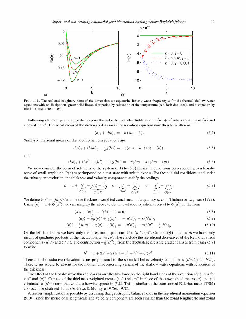
Figure 8 shows the real and imaginary parts of the complex frequency ω for the first few equatorial Rossby waves withn ∈ 1, 2, 3, and three different sets of κ and γ values. As before, the real part of ω is virtually unchanged by weakdissipation (κ = 0.002 or γ = 0.001) while Im(ω) becomes negative. The plot of Im(ω) in figure 8 closely resemblesour earlier figure 7, with the same apparent symmetry, if we now take κ = 2γ. A similar perturbation analysis to beforeshows that including this factor of 2 indeed makes Im(ω) symmetric about −ε/2 between the cases of small radiativerelaxation (κ = 2ε and γ = 0) and small friction (κ = 0 and γ = ε).

5. Acceleration of the zonal mean zonal flowWe now investigate the acceleration of the zonal mean zonal flow caused by these solutions for decaying equatorially

trapped Rossby waves.

5.1. Shallow water equations with thickness relaxation

We consider the shallow water model (1.1) with radiative relaxation of the thickness, and no forcing, on an equatorialbeta-plane, and apply the nondimensionalisation from §4.1 to obtain

ht + (hu)x + (hv)y = −κ(h− 1), (5.1)

(hu)t +(hu2 + 1

2h2)x

+ (huv)y −12yhv = −γhu− κu (h− 1) , (5.2)

(hv)t + (huv)x +(hv2 + 1

2h2)y

+ 12yhu = −γhv − κv (h− 1) . (5.3)

The mean thickness h0 becomes unity under this nondimensionalisation.


(a)

0 5 10

−0.2

−0.15

−0.1

−0.05

0

k

Re

(ω)

n=1

n=2

n=3

(b)

0 5 10

−10

−8

−6

−4

−2

0

x 10−4

k

Im(ω

)

κ = 0, γ = 0

κ = 0.002, γ = 0

κ = 0, γ = 0.001

FIGURE 8. The real and imaginary parts of the dimensionless equatorial Rossby wave frequency ω for the thermal shallow waterequations with no dissipation (green solid lines), dissipation by relaxation of the temperature (red dash-dot lines), and dissipation byfriction (blue dotted lines).

Following standard practice, we decompose the velocity and other fields as u = 〈u〉+ u′ into a zonal mean 〈u〉 anda deviation u′. The zonal mean of the dimensionless mass conservation equation may then be written as

〈h〉t + 〈hv〉y = −κ (〈h〉 − 1) . (5.4)

Similarly, the zonal means of the two momentum equations are

〈hu〉t + 〈huv〉y − 12y〈hv〉 = −γ〈hu〉 − κ (〈hu〉 − 〈u〉) , (5.5)

and

〈hv〉t + 〈hv2 + 12h

2〉y + 12y〈hu〉 = −γ〈hv〉 − κ (〈hv〉 − 〈v〉) . (5.6)

We now consider the form of solutions to the system (5.1) to (5.3) for initial conditions corresponding to a Rossbywave of small amplitude O(a) superimposed on a rest state with unit thickness. For these initial conditions, and underthe subsequent evolution, the thickness and velocity components satisfy the scalings

h = 1 + h′︸︷︷︸O(a)

+ (〈h〉 − 1)︸︷︷︸O(a2)

, u = u′︸︷︷︸O(a)

+ 〈u〉︸︷︷︸O(a2)

, v = v′︸︷︷︸O(a)

+ 〈v〉︸︷︷︸O(a2)

. (5.7)

We define 〈η〉∗ = 〈hη〉/〈h〉 to be the thickness-weighted zonal mean of a quantity η, as in Thuburn & Lagneau (1999).Using 〈h〉 = 1 +O(a2), we can simplify the above to obtain evolution equations correct to O(a2) in the form

〈h〉t + 〈v〉∗y + κ (〈h〉 − 1) = 0, (5.8)

〈u〉∗t − 12y〈v〉

∗ + γ〈u〉∗ = −〈u′v′〉y − κ〈h′u′〉, (5.9)

〈v〉∗t + 12y〈u〉

∗ + γ〈v〉∗ + 〈h〉y = −〈v′v′〉y − κ〈h′v′〉 − 12 〈h′2〉y. (5.10)

On the left hand sides we have only the three mean quantities 〈h〉, 〈u〉∗, 〈v〉∗. On the right hand sides we have onlymeans of quadratic products of the fluctuations h′, u′, v′. These include the meridional derivatives of the Reynolds stresscomponents 〈u′v′〉 and 〈v′v′〉. The contribution − 1

2 〈h′2〉y from the fluctuating pressure gradient arises from using (5.7)

to write

h2 = 1 + 2h′ + 2 (〈h〉 − 1) + h′2 +O(a3). (5.11)

There are also radiative relaxation terms proportional to the so-called bolus velocity components 〈h′u′〉 and 〈h′v′〉.These terms would be absent for the momentum-conserving variant of the shallow water equations with relaxation ofthe thickness.

The effect of the Rossby wave thus appears as an effective force on the right hand sides of the evolution equations for〈u〉∗ and 〈v〉∗. Our use of the thickness-weighted means 〈u〉∗ and 〈v〉∗ in place of the unweighted means 〈u〉 and 〈v〉eliminates a 〈h′v′〉 term that would otherwise appear in (5.8). This is similar to the transformed Eulerian mean (TEM)approach for stratified fluids (Andrews & McIntyre 1976a, 1978).

A further simplification is possible by assuming that geostrophic balance holds in the meridional momentum equation(5.10), since the meridional lengthscale and velocity component are both smaller than the zonal lengthscale and zonal


velocity component. The same scaling argument is used in the semigeostrophic theory of atmospheric front formation.The time derivative of this meridional geostrophic balance condition gives

12y〈u〉

∗t + 〈h〉yt = − 1

2 〈h′2〉yt, (5.12)

which can be used in place of (5.10) to obtain a closed system with (5.8) and (5.9).We now evaluate these right hand sides using the equatorially trapped Rossby wave solutions in §4.1. These rep-

resent small perturbations about a state of rest with unit depth in dimensionless variables. The meridional velocityperturbation is v′ = αRev(y) exp(i(kx − ωt)), with v(y) defined by (4.3) and (4.5), and the constant α sets theamplitude. The corresponding zonal velocity and thickness perturbations are u′ = αReu(y) exp(i(kx − ωt)) andh′ = αReh(y) exp(i(kx− ωt)), where

u(y) = i

(k (dv/dy)− 1

2y (ω + iκ) v

k2 − (ω + iγ) (ω + iκ)

), h(y) = −i

((iω − γ) u+ 1

2yv

k

), (5.13)

for k 6= 0. The denominator in the expression for u(y) vanishes when k2 = (ω + iγ) (ω + iκ). This gives the dispersionrelation for equatorially trapped Kelvin waves, which are distinguished by having zero meridional velocity (v = 0), andfrequencies ω = ±k in the absence of dissipation.

To allow a fair comparison between the effective forces generated by waves with different n and k values, we nor-malise the disturbance amplitudes by choosing α so that

1

2

∫〈u′2〉+ 〈v′2〉+ 〈h′2〉 dy = a2. (5.14)

The left hand side of (5.14) is the quadratic approximation to the disturbance pseudoenergy, an exact conserved quantityof the unforced, non-dissipative shallow water equations that takes the above form when expanded for small-amplitudedisturbances from a rest state of constant depth (Shepherd 1993). Using a standard formula for the average of a productof sinusoidal disturbances represented by the real parts of complex exponentials, we can compute the integrand in (5.14),and the terms on the right hand sides of (5.9) and (5.10), using

〈u′v′〉 = 12 Re

(u(y)v(y)†

)(5.15)

where the superscript † denotes a complex conjugate, and similarly for the other quadratic combinations of h′, u′, v′.Figures 9 and 10 show the two quantities −〈u′v′〉y and −κ〈h′u′〉 on the right hand side of (5.9), and their sum, for

waves with k = 1 and n ∈ 1, 2 for dissipation by either Rayleigh friction (γ > 0, κ = 0) or radiative relaxation(γ = 0, κ > 0). The plots show the quantities divided by a2, or equivalently correspond to setting a = 1. The Reynoldsstress 〈u′v′〉 vanishes for undamped waves, since ω, A, and v are then all real, while u and h are purely imaginary. Thebolus velocity term −κ〈h′u′〉 is explicitly proportional to κ, and so vanishes for κ = 0.

A perturbative analysis similar to that in §4.1 shows that the Reynolds stress 〈u′v′〉 is proportional to κ− γ for smallκ and γ. This explains the antisymmetry visible when comparing panel (a) with κ > 0, γ = 0 panel (b) with κ = 0,γ > 0 in each of figures 9 and 10. Increasing k while holding n, κ, γ fixed increases the magnitude of 〈u′v′〉 withoutchanging its general shape, as does increasing κ or γ while holding k and n fixed.

The Reynolds stress convergence is close to zero at the equator when n is odd, leaving just the contribution from thebolus velocity visible in figure 9(a). However, the Reynolds stress convergence has a local extremum on the equatorwhen n is even. Its sign for n = 2 is such as to produce eastward acceleration at the equator under radiative relaxation(figure 10(a)), and an westward acceleration at the equator under Rayleigh friction (figure 10(b)). We can infer the signof the acceleration directly from the right hand side of (5.9) on the equator. Since y = 0, the Coriolis contribution fromthe mean meridional velocity 〈v〉∗ does not contribute to the left hand side of (5.9). This leaves the ordinary differentialequation

d

dt〈u〉∗

∣∣y=0

+ γ〈u〉∗∣∣y=0

= −e−σt (〈u′v′〉y + κ〈h′u′〉)∣∣y=0,t=0

, (5.16)

where σ = −2Imω is twice the decay rate of the Rossby wave calculated in §4.1. The quadratic products on the righthand side of (5.9) thus decay in proportion to exp(−σt). The solution of (5.16) for γ 6= σ is

〈u〉∗∣∣y=0

=

[e−γt − e−σt

σ − γ

](〈u′v′〉y + κ〈h′u′〉)

∣∣y=0,t=0

, (5.17)

The time-dependent coefficient in square brackets [· · · ] is always positive for t > 0, so the direction of the zonal meanflow 〈u〉∗ at the equator is set by the sign of the combined Reynolds stress and bolus velocity term evaluated at y = 0and t = 0. This is consistent with the directions of the equatorial jets found in numerical simulations for different ratesof Rayleigh friction and radiative relaxation (Scott & Polvani 2007, 2008; Warneford & Dellar 2014).


However, away from the equator one would need to compute the solution to the full response problem coupling 〈h〉,〈u〉∗, 〈v〉∗ as three functions of y and t to find the mean flow produced by the wave sources on the right hand sides of(5.9) and (5.10). Figure 11 shows the three terms − 1

2 〈h′2〉y , −〈v′v′〉y and −κ〈h′u′〉 on the right hand side of (5.10),

and their sum, for k = 1, n ∈ 1, 2 and dissipation solely by radiative relaxation (κ = 0.001, γ = 0). The first twoterms are non-zero even with no dissipation, and typically much larger in magntitude than either the bolus terms or theReynolds stress convergence in the zonal equation.

Omitting the κ terms from the right hand sides of (5.2) and (5.3) leads to a shallow water model that relaxes thethickeness field but conserves momentum. This model is no less justified than the model that supposes that κ should notappear in the equation (1.1b) for evolving the velocity u. The contributions 〈h′u′〉 and 〈h′v′〉 from the bolus velocitywould then be absent in the right hand sides of the analogues of (5.9) and (5.10) for this model. Figures 9(a) and10(a) show that these contributions are in any case small compared with the contribution from the Reynolds stressconvergence. This is consistent with the directions of the equatorial jets in the two models, with and without momentumconservation, showing the same behaviour in simulations (Warneford & Dellar 2014).

5.2. Thermal shallow water equations

We now apply the same approach to the dimensionless form of the unforced thermal shallow water equations (1.2) onan equatorial beta plane. The mass and zonal momentum equations are

〈h〉t + 〈v〉∗y = 0, (5.18)

and

〈u〉∗t − 12y〈v〉

∗ + γ〈u〉∗ = −〈u′v′〉y. (5.19)

There are no κ terms in these equations, as radiative relaxation conserves mass and momentum in our thermal shallowwater model. The temperature Θ also does not appear in these equations, because the zonal pressure gradient disappearsunder zonal averaging.

To calculate the thermal contributions to the other equations, it is convenient to decompose the temperature as

Θ = 1 + θ = 1 + θ′︸︷︷︸O(a)

+ 〈θ〉︸︷︷︸O(a2)

. (5.20)

This decomposition eliminatesO(1) terms proportional to the reference temperature Θ0, which is scaled to unity by thenondimensionalisation in §4.2. Although θ′ = Θ′, we use θ′ below so that all equations are written using θ.

The meridional momentum equation is

(hv)t + (huv)x +(hv2 + 1

2h2(1 + θ)

)y

+ 12yhu = −γhv, (5.21)

and the conservation form of the temperature equation is

(hθ)t + (huθ)x + (hvθ)y = −κ(h2(1 + θ)− h

). (5.22)

The unit term from the decomposition Θ = 1 + θ disappears from the left hand side of (5.22) because h satisfies themass conservation equation with no source terms. However, the combination h2(1 + θ) appears in both the pressuregradient in (5.21) and the radiative relaxation term in (5.22). We may reduce this expression to a quadratic product bywriting

h2θ = hθ + h′θ′ +O(a3). (5.23)

The zonal mean of the temperature equation may thus be written as

〈θ〉∗t + κ (〈θ〉∗ + 〈h〉 − 1) = −〈v′θ′〉y − κ(〈h′θ〉+ 〈h′2〉

). (5.24)

As before for the velocity components, we use 〈θ〉∗ instead of 〈θ〉 to absorb a contribution from 〈θ′h′〉 in the timederivative. As θ = O(a) under our decomposition, we may neglect factors of 〈h〉 = 1+O(a2) that we could not neglectfor 〈Θ〉∗. Similarly, the zonal mean of the meridional momentum equation is

〈v〉∗t + 12y〈u〉

∗ + γ〈v〉∗ + 〈h〉y + 12 〈θ〉

∗y = −〈v′v′〉y − 1

2 〈h′2〉y − 1

2 〈h′θ′〉y, (5.25)

so we again have four equations for evolving 〈h〉, 〈u〉∗, 〈u〉∗, 〈θ〉∗ with linear left hand sides. The right hand sides areagain zonal means of quadratic products of the fluctuating quantities h′, u′, v′, θ′.

The meridional velocity perturbation for an equatorial Rossby wave is again v′ = αRev(y) exp(i(kx− ωt)), withv(y) defined by (4.3) and (4.10). The corresponding perturbations to the thickness, temperature, and zonal velocity take


(a)

−5 −2.5 0 2.5 5

x 10−4

−6

−4

−2

0

2

4

6

y

− 〈 u ′v ′〉 y

− κ 〈 h ′u ′ 〉t ot a l

(b)

−5 −2.5 0 2.5 5

x 10−4

−6

−4

−2

0

2

4

6

y

− 〈 u ′v ′〉 y

− κ 〈 h ′u ′〉t ot a l

FIGURE 9. The effective zonal forcing terms−〈u′v′〉y and−κ〈h′u′〉 on the right hand side of (5.9), and their sum, for (a) dissipationsolely by radiative relaxation (κ = 0.001, γ = 0) and (b) dissipation solely by friction (κ = 0, γ = 0.001). All terms are calculatedfor n = 1, k = 1, and a = 1 for scaling. Panel (b) has the sum equal to the first term as κ = 0.

(a)

−1 −0.5 0 0.5 1

x 10−3

−6

−4

−2

0

2

4

6

y

− 〈 u ′v ′〉 y

− κ 〈 h ′u ′ 〉t ot a l

(b)

−1 −0.5 0 0.5 1

x 10−3

−6

−4

−2

0

2

4

6

y

− 〈 u ′v ′〉 y

− κ 〈 h ′u ′〉t ot a l

FIGURE 10. The effective zonal forcing terms−〈u′v′〉y and−κ〈h′u′〉 on the right hand side of (5.9), and their sum, for (a) dissipationsolely by radiative relaxation (κ = 0.001, γ = 0) and (b) dissipation solely by friction (κ = 0, γ = 0.001). All terms are calculatedfor n = 2, k = 1, and a = 1 for scaling. Panel (b) has the sum equal to the first term as κ = 0.

(a) −0.2 0 0.2

−6

−4

−2

0

2

4

6

y

− 〈 v ′v ′ 〉 y

− 〈 h ′h ′ 〉 y

− κ 〈 h ′v ′ 〉t ot a l

(b) −0.2 0 0.2

−6

−4

−2

0

2

4

6

y

− 〈 v ′v ′ 〉 y

− 〈 h ′h ′ 〉 y

− κ 〈 h ′v ′ 〉t ot a l

FIGURE 11. The effective meridional forcing terms − 12〈h′2〉y , −〈v′v′〉y and −κ〈h′u′〉 on the right hand side of (5.10), and their

sum, for dissipation solely by radiative relaxation (κ = 0.001, γ = 0) and a = 1. All terms are calculated for k = 1 and either (a)n = 1 or (b) n = 2. The bolus velocity term −κ〈h′u′〉 is much smaller than the other two terms, which are not proportional to κ.


(a)

−5 0 5

x 10−4

−6

−4

−2

0

2

4

6

y

(b)

−5 −2.5 0 2.5 5

x 10−4

−6

−4

−2

0

2

4

6

y

FIGURE 12. The effective zonal force −〈u′v′〉y on the right hand side of (5.19) for k = 1, n = 1, and a = 1 for scaling.Panel (a) shows dissipation solely by radiative relaxation (κ = 0.002, γ = 0) and panel (b) shows dissipation solely by friction(κ = 0, γ = 0.001). The zero line is shown dotted. The ratio of κ to γ reflects the symmetry of the dispersion relation in §4.2.

(a)

−1 −0.5 0 0.5 1

x 10−3

−6

−4

−2

0

2

4

6

y

(b)

−1 −0.5 0 0.5 1

x 10−3

−6

−4

−2

0

2

4

6

y

FIGURE 13. The effective zonal force −〈u′v′〉y on the right hand side of (5.19) for k = 1, n = 2, and a = 1 for scaling.Panel (a) shows dissipation solely by radiative relaxation (κ = 0.002, γ = 0) and panel (b) shows dissipation solely by friction(κ = 0, γ = 0.001). The zero line is shown dotted. The ratio of κ to γ reflects the symmetry of the dispersion relation in §4.2.

the same functional forms, with

h(y) = −i

(iku+ dv/dy

ω

), Θ(y) = −i

(κh

ω + iκ

),

u(y) = i

(k (1 + iκ/ (2ω)) dv/dy − 1

2y (ω + iκ) v

k2 (1 + iκ/ (2ω))− (ω + iγ) (ω + iκ)

), (5.26)

for ω 6= 0 and ω 6= −iκ. The vanishing denominator in the expression for uwhen k2 = (ω + iγ) (ω + iκ) / (1 + iκ/ (2ω))again gives the dispersion relation for the equatorially trapped Kelvin waves. We choose the normalisation constant αso that the disturbances u′, v′, h′ and θ′ satisfy

1

2

∫〈u′2〉+ 〈v′2〉+ 〈(h′ + 1

2θ′)2〉 dy = a2. (5.27)

The left hand side is the dimensionless quadratic approximation for small amplitude disturbances to the pseudoenergy

1

2

∫h(u2 + v2

)+(h√

Θ− h0√

Θ0

)2dx dy (5.28)

for finite amplitude disturbances from a rest state of constant depth h0 and temperature Θ0 in the thermal shallow waterequations (Ripa 1995; Røed 1997; Warneford & Dellar 2013)

Figures 12 and 13 show the Reynolds stress convergences on the right hand side of (5.19). These all closely resemblethose for the previous shallow water equations with radiative relaxation of the thickness. Thus the mean flow at the


(a) −0.2 0 0.2

−6

−4

−2

0

2

4

6

y

− 〈 v ′v ′ 〉 y

−

1

2〈 h′ 2 〉 y

−

1

2〈 h ′

θ′ 〉 y

t ot a l

(b) −0.2 0 0.2

−6

−4

−2

0

2

4

6

y

− 〈 v ′v ′ 〉 y

−

1

2〈 h′ 2 〉 y

−

1

2〈 h ′

θ′ 〉 y

t ot a l

FIGURE 14. The effective meridional forcing terms−〈v′v′′〉y ,− 12〈h′2〉y ,− 1

2〈h′θ′〉y on the right hand side of (5.25), and their sum,

for dissipation solely by radiative relaxation (κ = 0.002, γ = 0). All terms are calculated for k = 1, a = 1 for scaling, and either (a)n = 1 or (b) n = 2.

(a)

−2 −1 0 1 2

x 10−3

−6

−4

−2

0

2

4

6

y

− 〈 v ′θ ′ 〉 y

− κ 〈 h′ 2 〉− κ 〈 h ′θ ′ 〉t ot a l

(b)

−3 −2 −1 0 1 2

x 10−3

−6

−4

−2

0

2

4

6

y

− 〈 v ′θ ′ 〉 y

− κ 〈 h′ 2 〉− κ 〈 h ′θ ′ 〉t ot a l

FIGURE 15. The effective thermal terms−〈v′θ′〉y ,−κ〈h′θ′〉,−κ〈h′2〉 on the right hand side of (5.24), and their sum, for dissipationsolely by radiative relaxation (κ = 0.002, γ = 0). All terms are calculated for k = 1, a = 1 for scaling, and either (a) n = 1 or (b)n = 2.

equator (y = 0) is almost identical to that for the previous model, provided κ is rescaled by a factor of 2. A perturbativeanalysis similar to that in §4.1 shows that the Reynolds stress 〈u′v′〉 for this model is proportional to κ/2− γ for smallκ and γ.

Figure 14 shows the forcing terms in the right hand side of the mean meridional momentum equation (5.25). Thedominant terms,−〈v′v′〉y and− 1

2 〈h′2〉y are very similar to those in figure 11 for the shallow water model with relaxation

of the thickness. The thermal term − 12 〈h′θ′〉y is much smaller. Finally, figure 15 shows the forcing terms in the right

hand side of the mean temperature equation (5.24). These all vanish for dissipation solely by friction (κ = 0), sincethe temperature perturbation θ given by (5.26) then vanishes, so they are only shown for κ > 0 and γ = 0. As for themeridional velocity, the contribution from 〈h′θ′〉 is much smaller than the other contributions.

5.3. Discussion

Our simulation parameters imply a dimensionless radiative relaxation rate κ = 7.88×10−3 roughly 23 times larger thanour dimensionless frictional rate γ = 3.42 × 10−4. In §5.1 we established that the Reynolds stress 〈u′v′〉 in the meanzonal momentum equation is proportional to κ − γ (for thickness relaxation) or κ/2 − γ (for temperature relaxation)for small relaxation and friction rates. For κ γ, our theory thus suggests that 〈u〉∗ > 0 on the equator, consistentwith the super-rotating equatorial jet in simulations. Conversely, for the purely frictional case (κ = 0) our theory gives〈u〉∗ < 0 on the equator, again consistent with the sub-rotating equatorial jet in simulations. These conclusions hold forboth shallow water models, with either the thickness or the temperature being relaxed. The Reynolds stresses in the twomodels are very similar for small relaxation and friction rates, provided one rescales the radiative relaxation rate κ inthe thermal model by a factor of 2, as in figures 12(a) and 13(a).


We have performed a similar analysis for decaying equatorially trapped Kelvin, Yanai, and inertia-gravity waves inour two shallow water models with radiative relaxation of the thickness or temperature. The effective zonal forces due tothese waves are at least an order of magnitude smaller than those due to decaying Rossby waves of the same pseudoen-ergy. Thus, as expected from our global QG simulations, these other types of wave make no significant contribution tosetting the direction of the equatorial jet.

Our thermal shallow water model conserves both mass and momentum in the absence of friction (γ = 0). This offers asimple demonstration that there is no inconsistency between our calculations of positive (eastward) zonal accelerationsat the equator due to radiative dissipation of Rossby waves and the arguments of §2 that Rossby waves should carrywestward pseudomomentum. The evolution equation for u may be rewritten in conservation form as

∂t(h(u− y2/4)

)+ ∂x

((hu(u− y2/4) + Θh2/2

)+ ∂y

(hv(u− y2/4)

)= 0. (5.29)

The combination u− y2/4 corresponds to the zonal velocity seen in an inertial frame, such that ∂xv− ∂y(u− y2/4) =y/2 + ∂xv − ∂yu is the absolute vorticity (Ripa 1993). The combination h(u− y2/4), sometimes called absolute zonalmomentum, is the beta-plane analogue of azimuthal angular momentum in spherical geometry.

The zonal mean of (5.29) is

∂t⟨h(u− y2/4)

⟩+ ∂y

⟨hv(u− y2/4)

⟩= 0, (5.30)

which becomes

∂t(〈u〉∗ − 1

4y2〈h〉

)+ ∂y

(〈u′v′〉 − 1

4y2〈hv〉

)= 0, (5.31)

correct to O(a2). Integrating (5.31) over y implies that the global absolute zonal momentum

M =

∫ ∞−∞

dy 〈u〉∗ − 14y

2(〈h〉 − 1) (5.32)

is constant in time. We have added the time-independent term y2/4 to the integrand defining M so that this integralconverges when 〈h〉 → 1 as y → ±∞. EvaluatingM at t = 0 for the equatorially trapped Rossby wave solution from§4.2 for which 〈h〉 = 1 and 〈u〉 = 0 initially, we obtain

M∣∣∣∣t=0

=

∫ ∞−∞

dy 12Reh(y)u(y)∗ < 0, (5.33)

where h(y) and u(y) are defined in (5.26), and v(y) is defined by (4.3) and (4.10). This negative sign agrees with thesign of the total zonal momentum due to a Rossby wave, as described in §2.

The mass-weighted mean zonal velocity 〈u〉∗ generated by the decaying Rossby wave may be positive (eastward) atthe equator, but the meridional integral of 〈u〉∗ − 1

4y2(〈h〉 − 1) that definesM is still negative (westward). This is all

that is required to reconcile conservation of zonal angular momentum with the requirement that Rossby waves shouldcarry westward zonal pseudomomentum, as established concretely by (5.33).

6. ConclusionsNumerical simulations of shallow water equations on a sphere with isotropic random forcing reliably produce a

mix of coherent vortices and alternating zonal jets. These simulations typically include Rayleigh friction to absorb thegradual inverse cascade of energy past the Rhines scale, since the zonal jets would otherwise break up into domain-sized coherent vortices after very long times. Such simulations invariably produce sub-rotating equatorial jets when runwith Jovian parameters (Vasavada & Showman 2005). However, simulations that model radiative effects by relaxing thethickness field produce a super-rotating equatorial jet (Scott & Polvani 2007, 2008), as do simulations of the thermalshallow water equations with a radiative relaxation term in the temperature equation (see §3 and Warneford & Dellar2014).

We have provided a possible explanation for the different directions of the equatorial jets in different shallow watermodels with dissipation by Rayleigh friction or Newtonian radiative relaxation. We formulated evolution equations forthe zonal mean thickness 〈h〉, and the thickness-weighted zonal mean quantities 〈u〉∗, 〈v〉∗, 〈θ〉∗. These equations con-tain effective forces due to zonal means of products of fluctuations, such as the Reynolds stress convergence 〈u′v′〉y inthe evolution equation for 〈v〉∗. We evaluated these effective forces for an equatorially trapped Rossby waves superim-posed on a background rest state on an equatorial beta plane. Dissipation changes the usual phase relations between theperturbations u′, v′, h′, and permits a nonzero Reynolds stress 〈u′v′〉 that transports zonal momentum in the meridionaldirection. This Reynolds stress is proportional to κ − γ for the shallow water model with relaxation of the thickness,and to κ/2− γ for the thermal shallow water model with relaxation of the temperature. The Reynolds stress divergence〈u′v′〉y is the sole forcing term in the momentum-conserving shallow water models, and the larger forcing term in the


Scott & Polvani (2007, 2008) model with radiative relaxation of both thickness and momentum. In all cases, radiative re-laxation produces a Reynolds stress with the opposite sign to that due to Rayleigh friction. This suffices to determine thatthe zonal mean flow 〈u〉∗ on the equator created by the decaying Rossby wave with n = 2 is eastward (super-rotating)for dissipation by radiative relaxation, and westward (sub-rotating) for dissipation by Rayleigh friction.

Our work relies upon several major simplifying assumptions. We considered trapped equatorial Rossby waves on abackground rest state, which allowed us to use the known analytical expressions for these waves in terms of Hermitepolynomials. A more complete theory would calculate the Rossby wave spectrum supported by a zonally symmetricbackground flow. Secondly, we only calculated the effective forces in the evolution equations for the thickness-weightedzonal mean quantities 〈u〉∗, 〈v〉∗, 〈θ〉∗. This is only sufficient to determine the evolution of 〈u〉∗ at the equator. Else-where, one would need to solve the system of three or four coupled equations to determine the Coriolis contributionto 〈u〉∗ from 〈v〉∗. However, it is worth noting that the latitude-dependence of the Reynolds stress divergence 〈u′v′〉yfor the n = 1 equatorially trapped Rossby wave, with two local maxima around y = ±1 in figures 9(a) and 12(a), issuggestive of the presence of two “horns”, peaks of maximal eastward velocity, at latitudes around ±7 near the edgesof the broad Jovian equatorial jet, and a slightly smaller velocity precisely on the equator (see figure 1).

Finally, we assumed that the waves are excited by sources outside the equatorial region, and neglected the effect of thisexcitation on the zonal mean flow. Some support for this second assumption is offered by simulations of the quasilinearversion of the Scott & Polvani (2007, 2008) model in spherical geometry by Saito & Ishioka (2014) which show thatthe zonal mean zonal acceleration due to the ensemble of Rossby waves excited by random forcing of the wavenumbersin the annulus described in §3, and decaying by either radiative relaxation or friction, produce an equatorial jet inthe direction predicted by our arguments, and with an amplitude consistent at early times with their fully nonlinearsimulations. They also gave an elegant argument to determine the direction of the zonal acceleration from the tilting ofthe constant phase lines in the separable Rossby wave solutions, as previously demonstrated by Andrews & McIntyre(1976b) for stratified fluids, and later adapted to shallow water models by Mofjeld (1981) and Yamagata & Philander(1985). Although our work falls short of a full wave-mean flow interaction theory, we believe it offers at least a steptowards a theoretical explanation of the origins of equatorial super- or sub-rotation in shallow water simulations ofJovian atmospheres.

We thank Michael McIntyre for very detailed and stimulating referee reports that greatly improved our manuscript,and Rick Salmon and Ted Johnson for useful conversations. This work was supported by the Engineering and PhysicalSciences Research Council through a Doctoral Training Grant award to E.S.W. and an Advanced Research Fellowshipto P.J.D. [grant number EP/E054625/1]. The computations employed the University of Oxford’s Advanced ResearchComputing facilities (Richards 2015), and the Emerald GPU-accelerated High Performance Computer made availableby the Science and Engineering South Consortium in partnership with the Science and Technology Facilities Council’sRutherford–Appleton Laboratory.

REFERENCES

ANDREWS, D. & MCINTYRE, M. 1976a Planetary waves in horizontal and vertical shear: The generalized Eliassen–Palm relationand the mean zonal acceleration. J. Atmos. Sci. 33, 2031–2048.

ANDREWS, D. & MCINTYRE, M. 1976b Planetary waves in horizontal and vertical shear: Asymptotic theory for equatorial wavesin weak shear. J. Atmos. Sci. 33, 2049–2053.

ANDREWS, D. G. & MCINTYRE, M. E. 1978 Generalized Eliassen–Palm and Charney–Drazin theorems for waves on axisymmetricmean flows in compressible atmospheres. J. Atmos. Sci. 35, 175–185.

BEEBE, R. 1994 Characteristic zonal winds and long-lived vortices in the atmospheres of the outer planets. Chaos 4, 113–122.BUHLER, O. 2000 On the vorticity transport due to dissipating or breaking waves in shallow-water flow. J. Fluid Mech. 407, 235–263.BUHLER, O. 2014 Waves and Mean Flows, 2nd edn. Cambridge: Cambridge University Press.CHARNEY, J. G. 1949 On a physical basis for numerical prediction of large-scale motions in the atmosphere. J. Atmos. Sci. 6,

372–385.CHO, J. Y.-K. & POLVANI, L. M. 1996a The emergence of jets and vortices in freely evolving, shallow-water turbulence on a

sphere. Phys. Fluids 8, 1531–1552.CHO, J. Y.-K. & POLVANI, L. M. 1996b The morphogenesis of bands and zonal winds in the atmospheres on the giant outer planets.

Science 273, 335–337.DALEY, R. 1983 Linear non-divergent mass-wind laws on the sphere. Tellus A 35A, 17–27.DICKINSON, R. E. 1969 Theory of planetary wave-zonal flow interaction. J. Atmos. Sci. 26, 73–81.DOWLING, T. E. 1995 Estimate of Jupiter’s deep zonal-wind profile from Shoemaker–Levy 9 data and Arnol’d’s second stability

criterion. Icarus 117, 439–442.DOWLING, T. E. & INGERSOLL, A. P. 1989 Jupiter’s Great Red Spot as a shallow water system. J. Atmos. Sci. 46, 3256–3278.GILL, A. E. 1982 Atmosphere Ocean Dynamics. New York: Academic Press.


GREEN, J. S. A. 1970 Transfer properties of the large-scale eddies and the general circulation of the atmosphere. Q. J. R. Meteorol.Soc. 96, 157–185.

HAYNES, P. H. & MCINTYRE, M. E. 1990 On the conservation and impermeability theorems for potential vorticity. J. Atmos. Sci.47, 2021–2031.

HELD, I. M. 2000 The General Circulation of the Atmosphere: Superrotation. Lectures presented at the 2000 Geophysical FluidDynamics Summer Program, Woods Hole Oceanographic Institution, Woods Hole, MA, available from http://www.whoi.edu/page.do?pid=13076.

HIRST, A. C. 1986 Unstable and damped equatorial modes in simple coupled ocean-atmosphere models. J. Atmos. Sci. 43, 606–632.HOU, T. Y. & LI, R. 2007 Computing nearly singular solutions using pseudo-spectral methods. J. Comp. Phys. 226, 379–397.HUPCA, I. O., FALCOU, J., GRIGORI, L. & STOMPOR, R. 2012 Spherical harmonic transform with GPUs. Lecture Notes in Com-

puter Science 7155, 355–366.IACONO, R., STRUGLIA, M. V. & RONCHI, C. 1999a Spontaneous formation of equatorial jets in freely decaying shallow water

turbulence. Phys. Fluids 11, 1272–1274.IACONO, R., STRUGLIA, M. V., RONCHI, C. & NICASTRO, S. 1999b High-resolution simulations of freely decaying shallow-water

turbulence on a rotating sphere. Il Nuovo Cimento C 22, 813–821.INGERSOLL, A. P. 1990 Atmospheric dynamics of the outer planets. Science 248, 308–315.INGERSOLL, A. P., DOWLING, T. E., GIERASCH, P. J., ORTON, G. S., READ, P. L., SANCHEZ-LAVEGA, A., SHOWMAN, A. P.,

SIMON-MILLER, A. A. & VASAVADA, A. R. 2007 Dynamics of Jupiter’s atmosphere. In Jupiter: The Planet, Satellites andMagnetosphere (ed. F. Bagenal, T. E. Dowling & W. B. McKinnon), pp. 105–128. Cambridge: Cambridge University Press.

JUCKES, M. 1989 A shallow water model of the winter stratosphere. J. Atmos. Sci. 46, 2934–2956.KHOUIDER, B., MAJDA, A. J. & STECHMANN, S. N. 2013 Climate science in the tropics: waves, vortices and PDEs. Nonlinearity

26, R1–R68.LAVOIE, R. L. 1972 A mesoscale numerical model of lake-effect storms. J. Atmos. Sci. 29, 1025–1040.LIMAYE, S. S. 1986 Jupiter: New estimates of the mean zonal flow at the cloud level. Icarus 65, 335–352.LIU, J. & SCHNEIDER, T. 2010 Mechanisms of jet formation on the giant planets. J. Atmos. Sci. 67, 3652–3672.MAJDA, A. J. & KLEIN, R. 2003 Systematic multiscale models for the tropics. J. Atmos. Sci. 60, 393–408.MARCUS, P. S. 1988 Numerical simulation of Jupiter’s Great Red Spot. Nature 331, 693–696.MATSUNO, T. 1966 Quasi-geostrophic motions in the equatorial area. J. Meteorol. Soc. Japan 44, 25–43.MATSUNO, T. 1970 Vertical propagation of stationary planetary waves in the winter northern hemisphere. J. Atmos. Sci. 27, 871–883.MATSUNO, T. 1971 A dynamical model of the stratospheric sudden warming. J. Atmos. Sci. 28, 1479–1494.MCCREARY, J. P. 1985 Modeling equatorial ocean circulation. Annu. Rev. Fluid Mech. 17, 359–409.MCCREARY, J. P., FUKAMACHI, Y. & KUNDU, P. K. 1991 A numerical investigation of jets and eddies near an eastern ocean

boundary. J. Geophys. Res. 96, 2515–2534.MCCREARY, J. P. & KUNDU, P. K. 1988 A numerical investigation of the Somali Current during the Southwest Monsoon. J. Marine

Res. 46, 25–58.MCCREARY, J. P. & YU, Z. 1992 Equatorial dynamics in a 2 1

2-layer model. Prog. Oceanogr. 29, 61–132.

MCINTYRE, M. E. 1981 On the ‘wave momentum’ myth. J. Fluid Mech. 106, 331–347.MCINTYRE, M. E. & NORTON, W. A. 1990 Dissipative wave-mean interactions and the transport of vorticity or potential vorticity.

J. Fluid Mech. 212, 403–435.MOFJELD, H. O. 1981 An analytic theory on how friction affects free internal waves in the equatorial waveguide. J. Phys. Oceanogr.

11, 1585–1590.OBUKHOV, A. M. 1949 On the problem of the geostrophic wind. Izv. Akad. Nauk SSSR, Ser. Geograf. Geofiz. 13, 281–306.PHILANDER, S. G. H., YAMAGATA, T. & PACANOWSKI, R. C. 1984 Unstable air-sea interactions in the tropics. J. Atmos. Sci. 41,

604–613.POLVANI, L. M., WAUGH, D. W. & PLUMB, R. A. 1995 On the subtropical edge of the stratospheric surf zone. J. Atmos. Sci. 52,

1288–1309.PORCO, C. C., WEST, R. A., MCEWEN, A., DEL GENIO, A. D., INGERSOLL, A. P., THOMAS, P., SQUYRES, S., DONES, L.,

MURRAY, C. D., JOHNSON, T. V., BURNS, J. A., BRAHIC, A., NEUKUM, G., VEVERKA, J., BARBARA, J. M., DENK, T.,EVANS, M., FERRIER, J. J., GEISSLER, P., HELFENSTEIN, P., ROATSCH, T., THROOP, H., TISCARENO, M. & VASAVADA,A. R. 2003 Cassini imaging of Jupiter’s atmosphere, satellites, and rings. Science 299, 1541–1547.

RHINES, P. B. 1975 Waves and turbulence on a beta-plane. J. Fluid Mech. 69, 417–443.RICHARDS, A. 2015 University of Oxford Advanced Research Computing. Zenodo document doi:10.5281/zenodo.22558.RIPA, P. 1993 Conservation laws for primitive equations models with inhomogeneous layers. Geophys. Astrophys. Fluid Dynam. 70,

85–111.RIPA, P. 1995 On improving a one-layer ocean model with thermodynamics. J. Fluid Mech. 303, 169–201.RIPA, P. 1996a Low frequency approximation of a vertically averaged ocean model with thermodynamics. Rev. Mex. Fıs. 41, 117–

135.RIPA, P. 1996b Linear waves in a one-layer ocean model with thermodynamics. J. Geophys. Res. 101, 1233–1245.RØED, L. P. 1997 Energy diagnostics in a 1 1

2-layer, nonisopycnic model. J. Phys. Oceanogr. 27, 1472–1476.

RØED, L. P. & SHI, X. B. 1999 A numerical study of the dynamics and energetics of cool filaments, jets, and eddies off the IberianPeninsula. J. Geophys. Res. 104, 29817–29841.

SAITO, I. & ISHIOKA, K. 2014 Mechanism for the formation of equatorial superrotation in forced shallow-water turbulence withNewtonian cooling. J. Atmos. Sci. doi:10.1175/JAS-D-14-0235.1, in press.

SCHNEIDER, T. & LIU, J. 2009 Formation of jets and equatorial superrotation on Jupiter. J. Atmos. Sci. 66, 579–601.

http://www.whoi.edu/page.do?pid=13076

http://www.whoi.edu/page.do?pid=13076

doi:10.5281/zenodo.22558


SCHOPF, P. S. & CANE, M. A. 1983 On equatorial dynamics, mixed layer physics and sea surface temperature. J. Phys. 0ceanogr.13, 917–935.

SCHUBERT, W. H., TAFT, R. K. & SILVERS, L. G. 2009 Shallow water quasi-geostrophic theory on the sphere. J. Adv. Model.Earth Syst. 1, 2.

SCOTT, R. K. & POLVANI, L. M. 2007 Forced-dissipative shallow-water turbulence on the sphere and the atmospheric circulationof the giant planets. J. Atmos. Sci. 64, 3158–3176.

SCOTT, R. K. & POLVANI, L. M. 2008 Equatorial superrotation in shallow atmospheres. Geophys. Res. Lett. 35, L24202.SHEPHERD, T. G. 1993 A unified theory of available potential energy. Atmosphere-Ocean 31, 1–26.SHOWMAN, A. P. 2007 Numerical simulations of forced shallow-water turbulence: Effects of moist convection on the large-scale

circulation of Jupiter and Saturn. J. Atmos. Sci. 64, 3132–3157.SRINIVASAN, K. & YOUNG, W. R. 2012 Zonostrophic instability. J. Atmos. Sci. 69, 1633–1656.SRINIVASAN, K. & YOUNG, W. R. 2014 Reynolds stress and eddy diffusivity of β-plane shear flows. J. Atmos. Sci. 71, 2169–2185.THOMPSON, R. O. R. Y. 1971 Why there is an intense Eastward current in the North Atlantic but not in the South Atlantic. J. Phys.

Oceanogr. 1, 235–237.THUBURN, J. & LAGNEAU, V. 1999 Eulerian mean, contour integral, and finite-amplitude wave activity diagnostics applied to a

single-layer model of the winter stratosphere. J. Atmos. Sci. 56, 689–710.VALLIS, G. K. 2006 Atmospheric and Oceanic Fluid Dynamics. Cambridge University Press.VASAVADA, A. R. & SHOWMAN, A. P. 2005 Jovian atmospheric dynamics: an update after Galileo and Cassini. Rep. Prog. Phys.

68, 1935–1996.VERKLEY, W. T. M. 2009 A balanced approximation of the one-layer shallow-water equations on a sphere. J. Atmos. Sci. 66, 1735–

1748.WALTERSCHEID, R. L., BRINKMAN, D. G. & SCHUBERT, G. 2000 Wave disturbances from the comet SL–9 impacts into Jupiter’s

atmosphere. Icarus 145, 140–146.WARNEFORD, E. S. 2014 The thermal shallow water equations, their quasi-geostrophic limit, and equatorial super-

rotation in Jovian atmospheres. DPhil thesis, University of Oxford, http://ora.ox.ac.uk/objects/uuid:6604fcac-afe6-4abe-8a6f-6a09de4f933f.

WARNEFORD, E. S. & DELLAR, P. J. 2013 The quasi-geostrophic theory of the thermal shallow water equations. J. Fluid Mech.723, 374–403.

WARNEFORD, E. S. & DELLAR, P. J. 2014 Thermal shallow water models of geostrophic turbulence in Jovian atmospheres. Phys.Fluids 26, 016603.

WILLIAMS, G. P. 1978 Planetary circulations: 1. Barotropic representation of Jovian and terrestrial turbulence. J. Atmos. Sci. 35,1399–1426.

WILLIAMS, G. P. & YAMAGATA, T. 1984 Geostrophic regimes, intermediate solitary vortices and Jovian eddies. J. Atmos. Sci. 41,453–478.

YAMAGATA, T. & PHILANDER, S. 1985 The role of damped equatorial waves in the oceanic response to winds. J. Oceanogr. Soc.Japan 41, 345–357.

http://ora.ox.ac.uk/objects/uuid:6604fcac-afe6-4abe-8a6f-6a09de4f933f

http://ora.ox.ac.uk/objects/uuid:6604fcac-afe6-4abe-8a6f-6a09de4f933f

Super- and sub-rotating equatorial jets in shallow … and sub-rotating equatorial jets in shallow...

Documents

Transcript of Super- and sub-rotating equatorial jets in shallow … and sub-rotating equatorial jets in shallow...