Sunday, June 10, 2018 7:34 PM

Talk in Munich Page 1

Sunday, June 10, 2018 7:36 PM

Talk in Munich Page 2

Sunday, June 10, 2018 7:39 PM

Talk in Munich Page 3

Sunday, June 10, 2018 7:41 PM

Talk in Munich Page 4

Sunday, June 10, 2018 7:46 PM

Talk in Munich Page 5

Sunday, June 10, 2018 7:49 PM

Talk in Munich Page 6

On the maximal numerical range of some matrices.I

Ali N. Hameda, Ilya M. Spitkovskya,∗

aDivision of Science and Mathematics, New York University Abu Dhabi (NYUAD),Saadiyat Island, P.O. Box 129188 Abu Dhabi, United Arab Emirates

Abstract

The maximal numerical range W0(A) of a matrix A is the (regular) numericalrange W (B) of its compression B onto the eigenspace L of A∗A correspondingto its maximal eigenvalue. So, always W0(A) ⊆ W (A). We establish condi-tions under which W0(A) has a non-empty intersection with the boundary ofW (A), in particular, when W0(A) = W (A). We also describe W0(A) explic-itly for matrices unitarily similar to direct sums of 2-by-2 blocks, and providesome insight into the behavior of W0(A) when L has codimension one.

Keywords: Numerical range, Maximal numerical range, Normaloidmatrices

2000 MSC: 15A60 15A57

1. Introduction

Let Cn stand for the standard n-dimensional inner product space overthe complex field C. Also, denote by Cm×n the set (algebra, if m = n) of allm-by-n matrices with the entries in C. We will think of A ∈ Cn×n as a linearoperator acting on Cn.

IThe results are partially based on the Capstone project of the first named authorunder the supervision of the second named author. The latter was also supported in partby Faculty Research funding from the Division of Science and Mathematics, New YorkUniversity Abu Dhabi.

∗Corresponding author.Email addresses: alinosher@nyu.edu (Ali N. Hamed), ims2@nyu.edu,

imspitkovsky@gmail.com (Ilya M. Spitkovsky)

Preprint submitted to ELA May 17, 2018

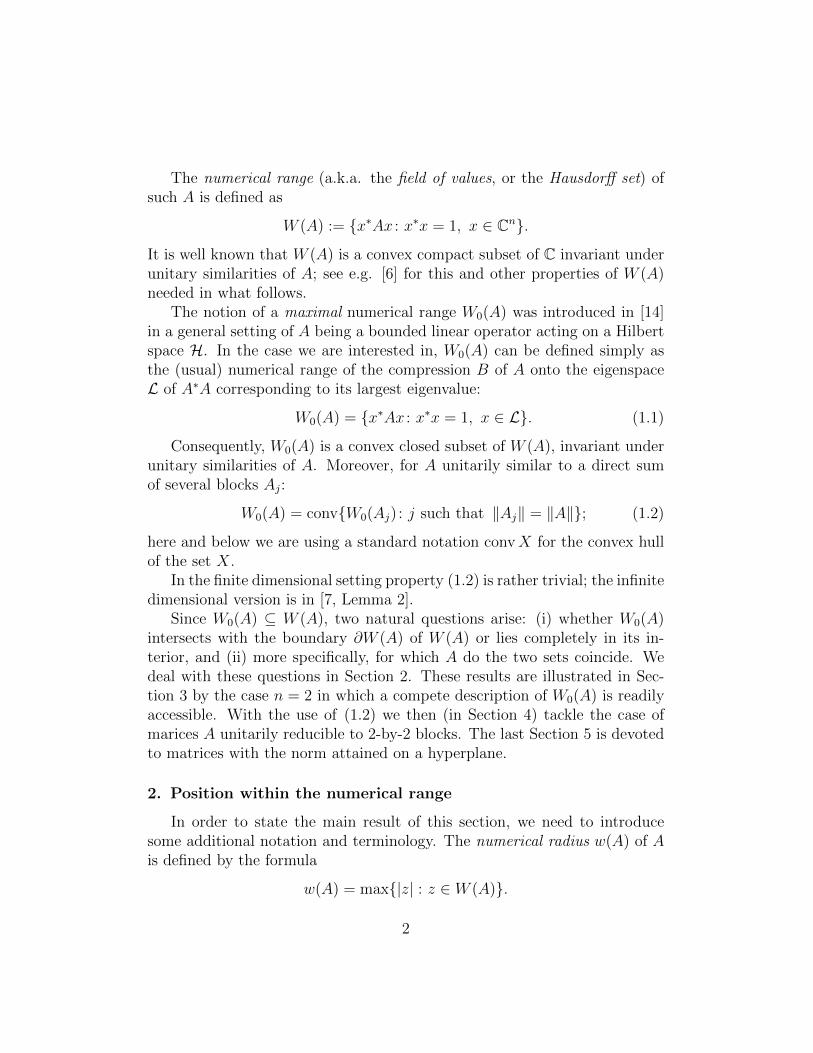
The numerical range (a.k.a. the field of values, or the Hausdorff set) ofsuch A is defined as

W (A) := {x∗Ax : x∗x = 1, x ∈ Cn}.

It is well known that W (A) is a convex compact subset of C invariant underunitary similarities of A; see e.g. [6] for this and other properties of W (A)needed in what follows.

The notion of a maximal numerical range W0(A) was introduced in [14]in a general setting of A being a bounded linear operator acting on a Hilbertspace H. In the case we are interested in, W0(A) can be defined simply asthe (usual) numerical range of the compression B of A onto the eigenspaceL of A∗A corresponding to its largest eigenvalue:

W0(A) = {x∗Ax : x∗x = 1, x ∈ L}. (1.1)

Consequently, W0(A) is a convex closed subset of W (A), invariant underunitary similarities of A. Moreover, for A unitarily similar to a direct sumof several blocks Aj:

W0(A) = conv{W0(Aj) : j such that ‖Aj‖ = ‖A‖}; (1.2)

here and below we are using a standard notation convX for the convex hullof the set X.

In the finite dimensional setting property (1.2) is rather trivial; the infinitedimensional version is in [7, Lemma 2].

Since W0(A) ⊆ W (A), two natural questions arise: (i) whether W0(A)intersects with the boundary ∂W (A) of W (A) or lies completely in its in-terior, and (ii) more specifically, for which A do the two sets coincide. Wedeal with these questions in Section 2. These results are illustrated in Sec-tion 3 by the case n = 2 in which a compete description of W0(A) is readilyaccessible. With the use of (1.2) we then (in Section 4) tackle the case ofmarices A unitarily reducible to 2-by-2 blocks. The last Section 5 is devotedto matrices with the norm attained on a hyperplane.

2. Position within the numerical range

In order to state the main result of this section, we need to introducesome additional notation and terminology. The numerical radius w(A) of Ais defined by the formula

w(A) = max{|z| : z ∈ W (A)}.

2

The Cauchy-Schwarz inequality implies that w(A) ≤ ‖A‖, and the equalityw(A) = ‖A‖ holds if and only if there is an eigenvalue λ of A with |λ| = ‖A‖,i.e., the norm of A coincides with its spectral radius ρ(A). If this is the case,A is called normaloid . In other words, A is normaloid if

Λ(A) := {λ ∈ σ(A) : |λ| = ‖A‖} (= {λ ∈ W (A) : |λ| = ‖A‖}) 6= ∅.

Theorem 1. Let A ∈ Cn×n. Then the following statements are equivalent:

(i) A is normaloid;

(ii) W0(A) ∩ ∂W (A) 6= ∅;(iii) {λ ∈ W0(A) : |λ| = ‖A‖} 6= ∅.

Proof. (i) ⇒ (iii). As was shown in [5], ρ(A) = ‖A‖ if and only if A isunitarily similar to a direct sum cU ⊕ B, where U is unitary, c is a positiveconstant and the block B (which may or may not be actually present) is suchthat ρ(B) < c, ‖B‖ ≤ c.

For such A we have ‖A‖ = ρ(A) = c, and according to (1.2):

W0(A) =

{W (cU) = conv Λ(A) if ‖B‖ < c,

conv(Λ(A) ∪W0(B)) otherwise.(2.1)

Either way, W0(A) ⊃ Λ(A).(iii)⇒ (ii). Since w(A) ≤ ‖A‖, the points of W (A) (in particular, W0(A))

having absolute value ‖A‖ automatically belong to ∂W (A).(ii) ⇒ (i). Considering A/ ‖A‖ in place of A itself, we may without loss

of generality suppose that ‖A‖ = 1. Pick a point a ∈ W0(A) ∩ ∂W (A). Bydefinition of W0(A), there exists a unit vector x ∈ Cn for which ‖Ax‖ = 1and x∗Ax = a. Choose also a unit vector y orthogonal to x, requiring inaddition that y ∈ Span{x,Ax} if x is not an eigenvector of A. Let C be thecompression of A onto the 2-dimensional subspace Span{x, y}. The matrix

A0 :=

[a bc d

]of C with respect to the orthonormal basis {x, y} then satisfies

|a|2 + |c|2 = 1. From here:

A∗0A0 =

[1 ab+ cd

ab+ cd |b|2 + |d|2]. (2.2)

But ‖A0‖ ≤ ‖A‖ = 1. Comparing this with (2.2) we conclude that

ab+ cd = 0. (2.3)

3

Moreover, W (A0) ⊂ W (A), and so a ∈ ∂W (A0). This implies |b| = |c|,as was stated explicitly in [16, Corollary 4] (see also [4, Proposition 4.3]).Therefore, (2.3) is only possible if b = c = 0 or |a| = |d|.

In the former case |a| = 1, immediately implying w(A) = 1 = ‖A‖.In the latter case, some additional reasoning is needed. Namely, then

|b|2 + |d|2 = |c|2 + |a|2 = 1 which in combination with (2.3) means that A0

is unitary. Since W (A) ⊃ σ(A0), we see that w(A) ≥ 1. On the other hand,w(A) ≤ ‖A‖ = 1, and so again w(A) = ‖A‖.

Note that Theorem 1 actually holds in the infinite-dimensional setting.For this (more general) situation, the equivalence (i) ⇔ (iii) was establishedin [2, Corollary 1], while (i) ⇔ (ii) is from [13]. Moreover, the paper [2]prompted [13]. The proof in the finite-dimensional case is naturally somewhatsimpler, and we provide it here for the sake of completeness.

If the matrix B introduced in the proof of Theorem 1 is itself normaloid,then ‖B‖ < c and W0(A) is given by the first line of (2.1). This is truein particular for normal A, when B is also normal. On the other hand, if‖B‖ = c, then Theorem 1 (applied to B) implies that W0(B) lies strictlyin the interior of W (B). In particular, there are no points in W (B) withabsolute value c(= ‖A‖). From here we immediately obtain

Corollary 1. For any A ∈ Cn×n,

{λ ∈ W0(A) : |λ| = ‖A‖} = Λ(A).

This is a slight refinement of condition (ii) in Theorem 1.

Theorem 2. Given a matrix A ∈ Cn×n, its numerical range and maximalnumerical range coincide if and only if A is unitarily similar to a direct sumcU ⊕B where U is unitary, c > 0, and W (B) ⊆ cW (U).

Proof. Sufficiency. Under the condition imposed on B, W (A) = cW (U). Atthe same time, W0(A) ⊇ W0(cU) = cW (U).

Necessity. If W (A) = W0(A), then in particular W0(A) has to intersect∂W (A), and by Theorem 1 A is normaloid. As such, A is unitarily similar tocU ⊕B with ‖B‖ ≤ c, ρ(B) < c. It was observed in the proof of Theorem 1that, if B itself is normaloid, then W0(A) = cW (U), and so we must haveW (A) = cW (U), implying W (B) ⊆ cW (U).

Consider now the case when B is not normaloid. If W (B) ⊆ cW (U)does not hold, draw a support line ` of W (B) such that cW (U) lies to the

4

same side of it as W (B) but at a positive distance from it. Since W (A) =conv(cW (U)∪W (B)), ` is also a support line of W (A). Meanwhile W0(B) iscontained in the interior of W (B), making the distance between W0(B) and `positive, and implying that ` is not a support line of conv(cW (U)∪W0(B)).According to (2.1), the latter set is the same as W0(A). Thus, W0(A) 6=W (A), which is a contradiction.

3. 2-by-2 matrices

A 2-by-2 matrix A is normaloid if and only if it is normal. The situationis then rather trivial: denoting σ(A) = {λ1, λ2} with |λ1| ≤ |λ2|, we haveW (A) = [λ1, λ2] (the line segment connecting λ1 with λ2), and

W0(A) =

{{λ2} 6= W (A) if |λ1| < |λ2| ,[λ1, λ2] = W (A) otherwise.

So, the only interesting case is that of a non-normal A. The eigenvalues ofA∗A are then simple, and W0(A) is therefore a point. According to Theo-rem 1, this point lies inside the ellipse W (A). Our next result is the formulafor its exact location.

Theorem 3. Let A ∈ C2×2 be not normal but otherwise arbitrary. ThenW0(A) = {z0}, where

z0 =(t0 − |λ2|2)λ1 + (t0 − |λ1|2)λ2

2t0 − trace(A∗A), (3.1)

λ1, λ2 are the eigenvalues of A, and

t0 =1

2

(trace(A∗A) +

√(trace(A∗A))2 − 4 |detA|2

). (3.2)

Note that an alternative form of (3.1),

z0 =t0 · traceA− (detA) · traceA

2t0 − trace(A∗A), (3.3)

without λj explicitly present, is sometimes more convenient.

5

Proof. Since both the value of z0 and the right-hand sides of formulas (3.1)–(3.3) are invariant under unitary similarities, it suffices to consider A in theupper triangular form

A =

[λ1 c0 λ2

], c > 0.

Then

1A∗A− tI =

[|λ1|2 − t cλ1cλ1 c2 + |λ2|2 − t

],

so the maximal eigenvalue t0 of A∗A satisfies

c2 |λ1|2 = (t0 − |λ1|2)(t0 − |λ2|2 − c2) (3.4)

and is thus given by formula (3.2). Choosing a respective eigenvector as

x =[cλ1, t0 − |λ1|2

]T,

we obtain successively

‖x‖2 = c2 |λ1|2 + (t0 − |λ1|2)2,

Ax =[ct0, (t0 − |λ1|2)λ2

]T,

x∗Ax = c2t0λ1 + (t0 − |λ1|2)2λ2,

and so finally

z0 =x∗Ax

‖x‖2=c2t0λ1 + (t0 − |λ1|2)2λ2c2 |λ1|2 + (t0 − |λ1|2)2

. (3.5)

To put this expression for z0 in form (3.1), we proceed as follows. Due to(3.4), the denominator in the right-hand side of (3.5) is nothing but

(t0 − |λ1|2)((t0 − |λ2|2 − c2) + (t0 − |λ1|2)

)= (t0 − |λ1|2)(2t0 − trace(A∗A)). (3.6)

On the other hand, also from (3.4),

c2t0 = (t0 − |λ1|2)(t0 − |λ2|2),

6

and the numerator in the right-hand side of (3.5) can be rewritten as

(t0 − |λ1|2)(t0 − |λ2|2)λ1 + (t0 − |λ1|2)λ2= (t0 − |λ1|2)

((t0 − |λ2|2)λ1 + (t0 − |λ1|2)λ2

). (3.7)

It remains to divide (3.7) by (3.6).

To interpret formula (3.1) geometrically, let us rewrite it as

z0 = t1λ1 + t2λ2,

where

t1 =t0 − |λ2|2

2t0 − trace(A∗A), t2 =

t0 − |λ1|2

2t0 − trace(A∗A).

According to (3.2), the denominator of these formulas can be rewrittenas√

(trace(A∗A))2 − 4 |detA|2 =

√(|λ1|2 + |λ2|2 + c2)2 − 4 |λ1λ2|2

=

√(|λ1|2 − |λ2|2)2 + 2c2(|λ1|2 + |λ2|2) + c4 > 0.

Also, t0 ≥ c2 + max{|λ1|2 , |λ2|2}, and

(t0 − |λ1|2) + (t0 − |λ2|2) = 2t0 − trace(A∗A) + c2 > 2t0 − trace(A∗A).

Consequently, t1, t2 > 0 and t1+t2 > 1, implying that in case of non-collinearλ1, λ2 (equivalently, λ1λ2 /∈ R) z0 lies in the sector spanned by λ1, λ2 and isseparated from the origin by the line passing through λ1, λ2.

If, on the other hand, λ1 and λ2 lie on the line passing through the origin,the point z0 also lies on this line. More specifically, the following statementholds.

Corollary 2. Let A be a non-normal 2-by-2 matrix, with the maximal nu-merical range W0(A) = {z0}. Then the point z0:

(i) is collinear with the spectrum σ(A) = {λ1, λ2} if and only if λ1λ2 ∈ R;

(ii) coincides with one of the eigenvalues of A if and only if the other oneis zero;

(iii) lies in the open interval with the endpoints λ1, λ2 if and only if λ1λ2 < 0;

7

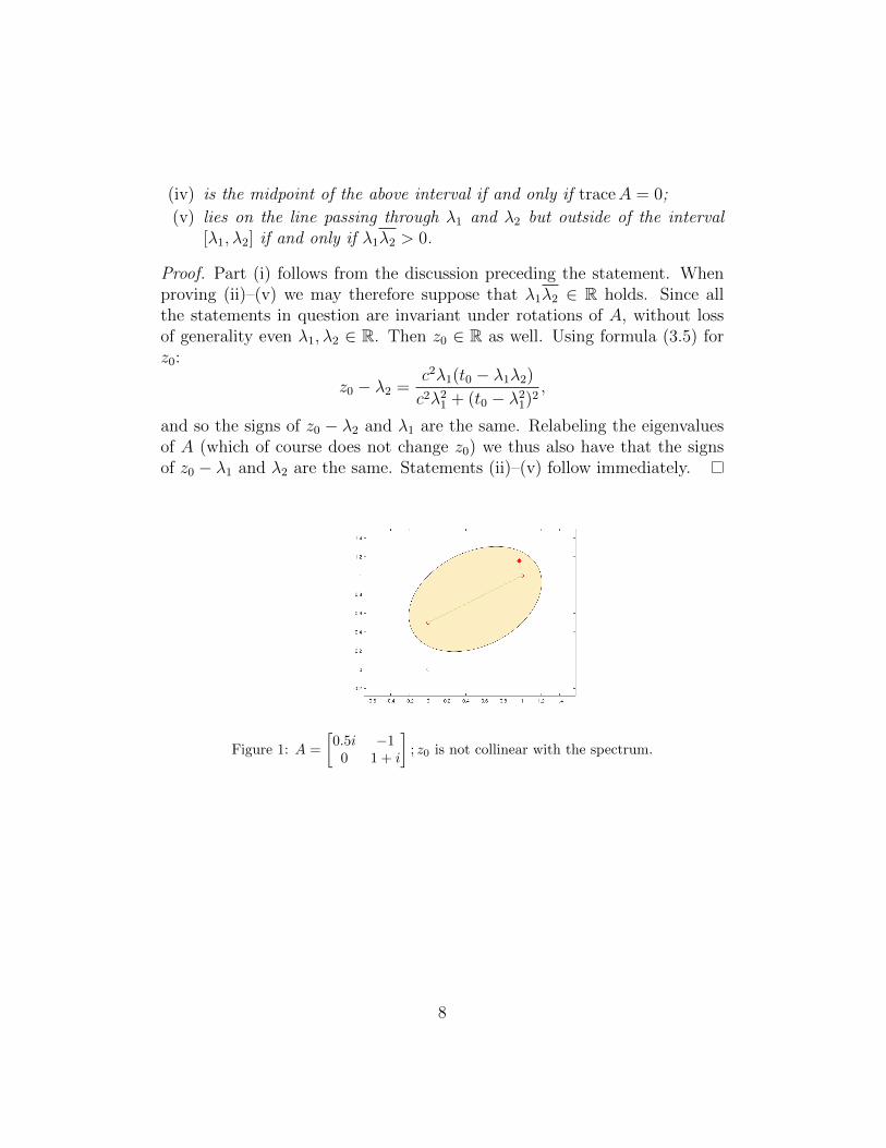
(iv) is the midpoint of the above interval if and only if traceA = 0;

(v) lies on the line passing through λ1 and λ2 but outside of the interval[λ1, λ2] if and only if λ1λ2 > 0.

Proof. Part (i) follows from the discussion preceding the statement. Whenproving (ii)–(v) we may therefore suppose that λ1λ2 ∈ R holds. Since allthe statements in question are invariant under rotations of A, without lossof generality even λ1, λ2 ∈ R. Then z0 ∈ R as well. Using formula (3.5) forz0:

z0 − λ2 =c2λ1(t0 − λ1λ2)c2λ21 + (t0 − λ21)2

,

and so the signs of z0 − λ2 and λ1 are the same. Relabeling the eigenvaluesof A (which of course does not change z0) we thus also have that the signsof z0 − λ1 and λ2 are the same. Statements (ii)–(v) follow immediately.

Figure 1: A =

[0.5i −1

0 1 + i

]; z0 is not collinear with the spectrum.

8

Figure 2: A =

[1 i0 0

]; z0 coincides with one of the eigenvalues since the other is zero.

Figure 3: A =

[−2 20 1

]; z0 is collinear with the spectrum and lies inside the interval

connecting it.

9

Figure 4: A =

[1 0.80 −1

]; z0 is the midpoint of the line connecting the eigenvalues.

Figure 5: A =

[2 0.750 1

]; z0 is collinear with the spectrum and lies outside the interval

connecting it.

4. Matrices decomposing into small blocks

A straightforward generalization of Theorem 3, based on Property (1.2),is the description of W0(A) for matrices A unitarily similar to direct sums of2-by-2 and 1-by-1 blocks.

Theorem 4. Let A be unitarily similar to

diag[λ1, . . . , λk]⊕ A1 ⊕ · · · ⊕ Am,

10

with Aj ∈ C2×2, j = 1, . . . ,m. Denote

tj =1

2

(trace(A∗jAj) +

√(trace(A∗jAj))

2 − 4 |detAj|2), (4.1)

zj =tj · traceAj − (detAj) · traceAj

2tj − trace(A∗A), j = 1, . . . ,m, (4.2)

t0 = max{tj, |λi|2 : i = 1, . . . , k; j = 1, . . . ,m},

and let I (resp. J) stand for the set of all i (resp. j) for which |λi|2 (resp.tj) equals t0. Then

W0(A) = conv{λi, zj : i ∈ I, j ∈ J}. (4.3)

According to (4.3), in the setting of Theorem 4, W0(A) is always a poly-gon.

Consider in particular A unitarily similar to[a1In1 XY a2In2

], (4.4)

with X ∈ Cn1×n2 and Y ∈ Cn2×n1 such that XY and Y X are both normal.As was shown in the proof of [1, Theorem 2.1], yet another unitary similaritycan be used to rewrite A as the direct sum of min{n1, n2} two-dimensionalblocks

Aj =

[a1 σjδj a2

](4.5)

and max{n1, n2}−min{n1, n2} one-dimensional blocks equal either a1 or a2.Here σj are the s-numbers of X, read from the diagonal of the middle term

in its singular value decomposition X = U1ΣU∗2 , while δj are the respective

diagonal entries of the matrix ∆ = U∗2Y U1, which can also be made diagonaldue to the conditions imposed on X, Y .

Since ‖Aj‖ ≥ max{|a1| , |a2|}, for matrices (4.4) (or unitarily similar tothem) formula (4.3) implies that W0(A) is the convex hull of zj given by (4.2)taken over those j only which deliver the maximal value of ‖Aj‖.

Here are some particular cases in which all zj, λi contributing to W0(A)happen to coincide. Then W0(A) is a singleton, as it was the case for 2-by-2matrices A different from scalar multiples of a unitary matrix.

11

Proposition 1. Let, in (4.4), a1 = −a2. Then W0(A) = {0}.

Proof. Indeed, in this case traceAj = 0, and formula (4.2) implies that zj = 0for all j, in particular for those with maximal ‖Aj‖ is attained.

Recall that a continuant matrix is by definition a tridiagonal matrix A ∈Cn×n such that its off-diagonal entries satisfy the requirement

ak,k+1 = −ak+1,k, k = 1, . . . , n− 1.

Such a matrix can be written as

C =

a1 b1 0 . . . 0

−b1 a2 b2. . .

...

0 −b2 a3. . . 0

.... . . . . . . . . bn−1

0 . . . 0 −bn−1 an

. (4.6)

Proposition 2. Let C be the continuant matrix (4.6) with a 2-periodic maindiagonal: a1 = a3 = . . . , a2 = a4 = . . .. Then W0(C) is a singleton.

Proof. Let T be the matrix with the columns e1, e3, . . . , e2, e4, . . ., where{e1, . . . , en} is the standard basis of Cn. It is easy to see that a unitarysimilarity performed by T transforms the continuant matrix (4.6) with the2-periodic main diagonal into the matrix (4.4) for which

X =

b1b2 b3

b4 b5. . . . . .

, Y = −X∗.

So, in (4.5) we have δj = −σj, and thus ‖Aj‖ depends monotonically onσj. The block on which the maximal norm is attained is therefore uniquelydefined (though might appear repeatedly), and the respective maximal valueof σj is nothing but ‖X‖.

It is clear from the proof of Proposition 2 how to determine the locationof W0(C): it is given by formulas (4.1), (4.2) with traceAj, trace(A∗jAj) and

detAj replaced by a1+a2, |a1|2+|a2|2+2 ‖X‖2, and a1a2+‖X‖2, respectively.

12

Finally, let A be quadratic, i.e., having the minimal polynomial of degreetwo. As is well known (and easy to show), A is then unitarily similar to amatrix [

λ1In1 X0 λ2In2

]. (4.7)

This fact was used e.g. in [15] to prove that for such matrices W (A) is thesame as W (A0), where A0 ∈ C2×2 is defined as

A0 =

[λ1 ‖X‖0 λ2

],

and thus W (A) is an elliptical disk.The next statement shows that the relation between A unitarily similar

to (4.7) and A0 persists when maximal numerical ranges are considered.

Proposition 3. Let A ∈ Cn×n be quadratic and thus unitarily similar to(4.7). Then W0(A) is a singleton {z0}, where

z0 =(‖A0‖2 − |λ2|2)λ1 + (‖A0‖2 − |λ1|2)λ2

2 ‖A0‖2 − (|λ1|2 + |λ2|2 + ‖X‖2).

Proof. Observe that (4.7) is a particular case of (4.4) in which Y = 0 andaj = λj, j = 1, 2. So, the normality of XY and Y X holds in a trivialway and, moreover, δj = 0 for all the blocks Aj appearing in the unitaryreduction of A. Similarly to the situation in Proposition 2, the norms ofAj depend monotonically on σj, and thus the maximum is attained on theblocks (of which there is at least one) coinciding with A0. It remains onlyto invoke formula (3.1), keeping in mind that t0 = ‖A0‖2 and trace(A∗0A0) =|λ1|2 + |λ2|2 + ‖X‖2.

In general, however, there is no reason for the set (4.3) to be a singleton.To illustrate, let A = A1 ⊕ A2 ⊕ A3, where

A1 =

[−1 1

1− i 2

], A2 =

[−1 1 + i1 2

], A3 =

[−1

√3+3√6

5

0 2

]. (4.8)

Then ‖Aj‖ =√

4 +√

6 for each j = 1, 2, 3, while W0(Aj) = {zj}, with

z1,2 ≈ 1.93∓ 0.20i, z3 ≈ 1.45. (4.9)

13

Figure 6: A is the direct sum of Aj given by (4.8). The maximal numerical range is thetriangle with the vertices zj given by (4.9).

5. Matrices with the norm attained on a hyperplane

Generically, the eigenvalues of A∗A are all distinct, and W0(A) is thereforea singleton. In more rigorous terms, the set of n-by-n matrices A with W0(A)being a point has the interior dense in Cn×n.

An opposite extreme is the case when A∗A has just one eigenvalue. Thishappens if and only if A is a scalar multiple of a unitary matrix — a simplesituation, covered by Theorem 2.

If n = 2, these are the only options, which is of course in agreementwith the description of W0(A) provided for this case in Section 3. Startingwith n = 3, however, the situation when the maximal eigenvalue of A∗Ahas multiplicity n− 1 becomes non-trivial. We here provide some additionalinformation about the shapes of W (A),W0(A) in this case.

The only way in which such matrices A can be unitarily reducible is ifthey are unitarily similar to cU ⊕ B, with U unitary and ‖B‖ = c attainedon a subspace of codimension one. Therefore, it suffices to consider the caseof unitarily irreducible A only.

To state the pertinent result, we need to recall one more notion. Namely,Γ is a Poncelet curve (of rank m with respect to a circle C) if it is a closedconvex curve lying inside C and such that for any point z ∈ C there is anm-gon inscribed in C, circumscribed around Γ, and having z as one of itsvertices.

14

Theorem 5. Let A ∈ Cn×n be unitarily irreducible, with the norm of Aattained on an (n−1)-dimensional subspace. Then ∂W (A) and ∂W0(A) bothare Poncelet curves (of rank n + 1 and n, respectively) with respect to thecircle {z : |z| = ‖A‖}.

Proof. Considering A/ ‖A‖ in place of A, we may without loss of generalitysuppose that C is the unit circle T, the matrix in question is a contractionwith ‖A‖ = 1 and rank(I − A∗A) = 1. Also, ρ(A) < 1 since otherwiseA would be normaloid and thus unitarily reducible. In the notation of [3](adopted in later publications), A ∈ Sn, and the result follows directly from[3, Theorem 2.1].

Moving to W0(A), consider the polar form UR of A. Since the statementin question is invariant under unitary similarities, we may suppose that thepositive semi-definite factor R is diagonalized. Condition rank(I−A∗A) = 1then implies that R = diag[1, . . . , 1, c], where 0 ≤ c < 1. In agreementwith (1.1), W0(A) = W (U0), where U0 is the matrix obtained from U bydeleting its last row and column. Note that U has no eigenvectors with thelast coordinate equal to zero, since otherwise they would also be eigenvectorsof R, implying unitary reducibility of A. In particular, the eigenvalues ofU are distinct. The statement now follows by applying [11, Theorem 1] toW (U0).

Note that the matrix U0 constructed in the second part of the proofactually belongs to Sn−1. The properties of W (T ) for T ∈ Sn stated in [3,Lemma 2.2] thus yield

Corollary 3. In the setting of Theorem 5, both ∂W (A) and ∂W0(A) aresmooth curves, with each point generated by exactly one (up to a unimodularscalar multiple) vector.

The above mentioned uniqueness of the generating vectors implies in par-ticular that ∂W (A), ∂W0(A) contain no flat portions.

To illustrate, consider the Jordan block Jn ∈ Cn×n corresponding to thezero eigenvalue. Then Jn ∈ Sn, with the norm of Jn attained on the spanL of the elements e2, . . . , en of the standard basis of Cn. Consequently, thecompression of Jn onto L is Jn−1, and W0(Jn) = W (Jn−1) is the circular disk{z : |z| ≤ cos π

n}, while W (Jn) is the (concentric but strictly larger) circular

disk {z : |z| ≤ cos πn+1}.

Finally, let us concentrate on the smallest size for which the situation ofthis Section is non-trivial, namely n = 3.

15

Proposition 4. A matrix A ∈ C3×3 is unitarily irreducible with the normattained on a 2-dimensional subspace if and only if it is unitarily similar to

ω

λ1√

(1− |λ1|2)(1− |λ2|2) −λ2√

(1− |λ1|2)(1− |λ3|2)

0 λ2

√(1− |λ2|2)(1− |λ3|2)

0 0 λ3

, (5.1)

where ω ∈ C \ {0}, −1 < λ2 ≤ 0, and |λj| < 1, j = 1, 3.

Proof. According to Schur’s lemma, we can put any A ∈ C3×3 in an uppertriangular form

A0 =

λ1 x y0 λ2 z0 0 λ3

. (5.2)

Further multiplication by an appropriate non-zero complex number w allowsus without loss of generality to suppose that ‖A‖ = 1 and xyz ≥ 0. Anadditional (diagonal) unitary similarity can then be used to arrange for x, y, zall to be non-negative. Being an irreducible contraction, the matrix (5.2) hasto satisfy |λj| < 1 (j = 1, 2, 3) and xz 6= 0. Rewriting the rank-one conditionfor I−A∗0A0 as the collinearity of its columns and solving the resulting systemof equations for x, y, z yields

x =

√(1− |λ1|2)(1− |λ2|2),

y =− λ2√

(1− |λ1|2)(1− |λ3|2),

z =

√(1− |λ2|2)(1− |λ3|2).

(5.3)

In particular, λ2 has to be non-positive, due to the non-negativity of y.Setting ω = w−1, we arrive at representation (5.1).A straightforward verification shows that the converse is also true, i.e.,

any matrix of the form (5.1) is unitarily irreducible with a norm attained ona 2-dimensional subspace.

Note that the form (5.1) can also be established by invoking [11, Theorem4], instead of solving for x, y, z in terms of λj straightforwardly.

In the setting of Proposition 4 the set W0(A) is the numerical range ofa 2-by-2 matrix, and in agreement with Corollary 3 is an elliptical disk. By

16

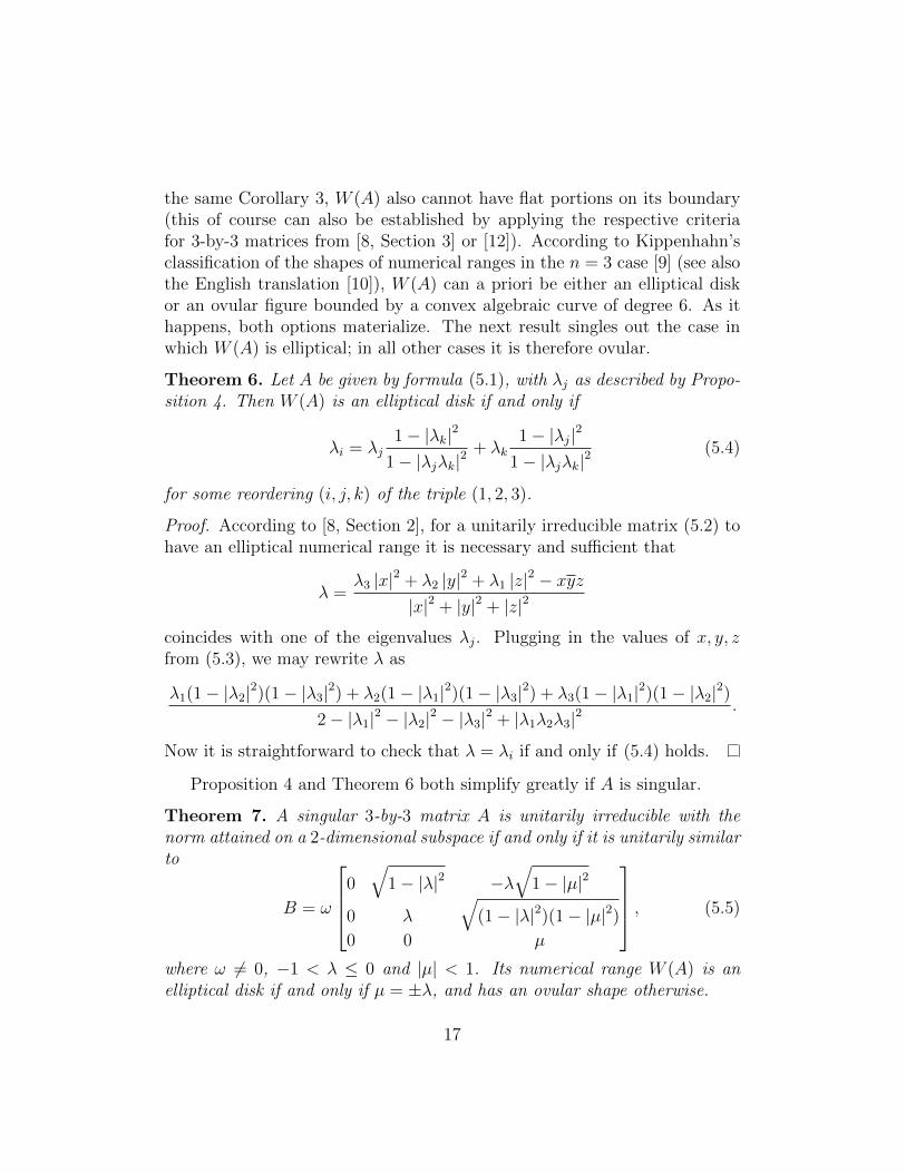
the same Corollary 3, W (A) also cannot have flat portions on its boundary(this of course can also be established by applying the respective criteriafor 3-by-3 matrices from [8, Section 3] or [12]). According to Kippenhahn’sclassification of the shapes of numerical ranges in the n = 3 case [9] (see alsothe English translation [10]), W (A) can a priori be either an elliptical diskor an ovular figure bounded by a convex algebraic curve of degree 6. As ithappens, both options materialize. The next result singles out the case inwhich W (A) is elliptical; in all other cases it is therefore ovular.

Theorem 6. Let A be given by formula (5.1), with λj as described by Propo-sition 4. Then W (A) is an elliptical disk if and only if

λi = λj1− |λk|2

1− |λjλk|2+ λk

1− |λj|2

1− |λjλk|2(5.4)

for some reordering (i, j, k) of the triple (1, 2, 3).

Proof. According to [8, Section 2], for a unitarily irreducible matrix (5.2) tohave an elliptical numerical range it is necessary and sufficient that

λ =λ3 |x|2 + λ2 |y|2 + λ1 |z|2 − xyz

|x|2 + |y|2 + |z|2

coincides with one of the eigenvalues λj. Plugging in the values of x, y, zfrom (5.3), we may rewrite λ as

λ1(1− |λ2|2)(1− |λ3|2) + λ2(1− |λ1|2)(1− |λ3|2) + λ3(1− |λ1|2)(1− |λ2|2)2− |λ1|2 − |λ2|2 − |λ3|2 + |λ1λ2λ3|2

.

Now it is straightforward to check that λ = λi if and only if (5.4) holds.

Proposition 4 and Theorem 6 both simplify greatly if A is singular.

Theorem 7. A singular 3-by-3 matrix A is unitarily irreducible with thenorm attained on a 2-dimensional subspace if and only if it is unitarily similarto

B = ω

0√

1− |λ|2 −λ√

1− |µ|2

0 λ√

(1− |λ|2)(1− |µ|2)0 0 µ

, (5.5)

where ω 6= 0, −1 < λ ≤ 0 and |µ| < 1. Its numerical range W (A) is anelliptical disk if and only if µ = ±λ, and has an ovular shape otherwise.

17

Note that for matrices (5.5) L = Span{e2, e3}, and so W0(B) is nothingbut the numerical range of the right lower 2-by-2 block of B. The next threefigures show the shape of W0(B) and W (B) for B given by (5.5) with ω = 1for several choices of λ, µ.

Figure 7: µ = λ = −2/5. The numerical range and maximal numerical range are bothcircular discs.

Figure 8: µ = −λ = 3/4. The numerical range and maximal numerical range are bothelliptical discs.

18

Figure 9: µ = 1/3, λ = −7/8. The numerical range is an ovular disc, and the maximalnumerical range is an elliptical disc.

References

[1] E. Brown and I. Spitkovsky, On matrices with elliptical numericalranges, Linear Multilinear Algebra 52 (2004), 177–193.

[2] Jor-Ting Chan and Kong Chan, An observation about normaloid oper-ators, Operators and Matrices 11 (2017), 885–890.

[3] Hwa-Long Gau and Pei Yuan Wu, Numerical range of S(φ), LinearMultilinear Algebra 45 (1998), no. 1, 49–73.

[4] , Numerical ranges and compressions of Sn-matrices, Operatorsand Matrices 7 (2013), no. 2, 465–476.

[5] M. Goldberg and G. Zwas, On matrices having equal spectral radius andspectral norm, Linear Algebra Appl. 8 (1974), 427–434.

[6] K. E. Gustafson and D. K. M. Rao, Numerical range. The field of valuesof linear operators and matrices, Springer, New York, 1997.

[7] Guoxing Ji, Ni Liu, and Ze Li, Essential numerical range and maximalnumerical range of the Aluthge transform, Linear Multilinear Algebra55 (2007), no. 4, 315–322.

[8] D. Keeler, L. Rodman, and I. Spitkovsky, The numerical range of 3× 3matrices, Linear Algebra Appl. 252 (1997), 115–139.

19

[9] R. Kippenhahn, Uber den Wertevorrat einer Matrix, Math. Nachr. 6(1951), 193–228.

[10] , On the numerical range of a matrix, Linear Multilinear Algebra56 (2008), no. 1-2, 185–225, Translated from the German by Paul F.Zachlin and Michiel E. Hochstenbach.

[11] B. Mirman, Numerical ranges and Poncelet curves, Linear Algebra Appl.281 (1998), 59–85.

[12] L. Rodman and I. M. Spitkovsky, 3× 3 matrices with a flat portion onthe boundary of the numerical range, Linear Algebra Appl. 397 (2005),193–207.

[13] I. M. Spitkovsky, A note on the maximal numerical range,arXiv.math.FA/1803.10516v1 (2018), 1–6.

[14] J. G. Stampfli, The norm of a derivation, Pacific J. Math. 33 (1970),737–747.

[15] Shu-Hsien Tso and Pei Yuan Wu, Matricial ranges of quadratic opera-tors, Rocky Mountain J. Math. 29 (1999), no. 3, 1139–1152.

[16] Hai-Yan Zhang, Yan-Ni Dou, Mei-Feng Wang, and Hong-Ke Du, On theboundary of numerical ranges of operators, Appl. Math. Lett. 24 (2011),no. 5, 620–622.

20