SUN RGB-D: A RGB-D Scene Understanding Benchmark Suite

Shuran Song Samuel P. Lichtenberg Jianxiong XiaoPrinceton University

http://rgbd.cs.princeton.edu

Abstract

Although RGB-D sensors have enabled major break-throughs for several vision tasks, such as 3D reconstruc-tion, we have not attained the same level of success in high-level scene understanding. Perhaps one of the main rea-sons is the lack of a large-scale benchmark with 3D anno-tations and 3D evaluation metrics. In this paper, we intro-duce an RGB-D benchmark suite for the goal of advancingthe state-of-the-arts in all major scene understanding tasks.Our dataset is captured by four different sensors and con-tains 10,335 RGB-D images, at a similar scale as PASCALVOC. The whole dataset is densely annotated and includes146,617 2D polygons and 64,595 3D bounding boxes withaccurate object orientations, as well as a 3D room layoutand scene category for each image. This dataset enablesus to train data-hungry algorithms for scene-understandingtasks, evaluate them using meaningful 3D metrics, avoidoverfitting to a small testing set, and study cross-sensorbias.

1. IntroductionScene understanding is one of the most fundamen-

tal problems in computer vision. Although remarkableprogress has been achieved in the past decades, general-purpose scene understanding is still considered to be verychallenging. Meanwhile, the recent arrival of affordabledepth sensors in consumer markets enables us to acquirereliable depth maps at a very low cost, stimulating break-throughs in several vision tasks, such as body pose recog-nition [56, 58], intrinsic image estimation [4], 3D modeling[27] and SfM reconstruction [72].

RGB-D sensors have also enabled rapid progress forscene understanding (e.g. [20, 19, 53, 38, 30, 17, 32, 49]).However, while we can crawl color images from the Inter-net easily, it is not possible to obtain large-scale RGB-Ddata online. Consequently, the existing RGB-D recogni-tion benchmarks, such as NYU Depth v2 [49], are an order-of-magnitude smaller than modern recognition datasets forcolor images (e.g. PASCAL VOC [9]). Although these

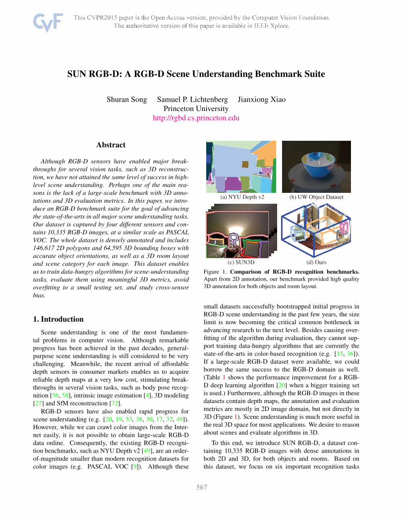
(a) NYU Depth v2 (b) UW Object Dataset

(c) SUN3D (d) OursFigure 1. Comparison of RGB-D recognition benchmarks.Apart from 2D annotation, our benchmark provided high quality3D annotation for both objects and room layout.

small datasets successfully bootstrapped initial progress inRGB-D scene understanding in the past few years, the sizelimit is now becoming the critical common bottleneck inadvancing research to the next level. Besides causing over-fitting of the algorithm during evaluation, they cannot sup-port training data-hungry algorithms that are currently thestate-of-the-arts in color-based recognition (e.g. [15, 36]).If a large-scale RGB-D dataset were available, we couldborrow the same success to the RGB-D domain as well.(Table 1 shows the performance improvement for a RGB-D deep learning algorithm [20] when a bigger training setis used.) Furthermore, although the RGB-D images in thesedatasets contain depth maps, the annotation and evaluationmetrics are mostly in 2D image domain, but not directly in3D (Figure 1). Scene understanding is much more useful inthe real 3D space for most applications. We desire to reasonabout scenes and evaluate algorithms in 3D.

To this end, we introduce SUN RGB-D, a dataset con-taining 10,335 RGB-D images with dense annotations inboth 2D and 3D, for both objects and rooms. Based onthis dataset, we focus on six important recognition tasks

1

Testing SetTraining Set

NYU (795 images) SUN RGB-D (5,285 images)

NYU 32.50 34.33SUN RGB-D 15.78 33.20

Table 1. Performance improves as the size of training data in-creases. We trained the Depth-RCNN [20] for 2D object detectionusing RGB-D images, and evaluated the mean average precision.Bigger training set produces better result. Especially for the firstrow using NYU as the testing set, the performance is still betterusing the bigger SUN RGB-D that is a superset of NYU, despitethe domain gap due to dataset bias.

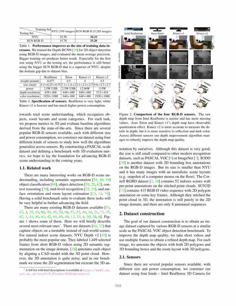
RealSense Xtion Kinect v1 Kinect v2weight (pound) 0.077 0.5 4 4.5

size (inch) 5.2×0.25×0.75 7.1×1.4×2 11×2.3×2.7 9.8×2.7×2.7power 2.5W USB 2.5W USB 12.96W 115W

depth resolution 628×468 640×480 640×480 512×424color resolution 1920×1080 640×480 640×480 1920×1080

Table 2. Specification of sensors. RealSense is very light, whileKinect v2 is heavier and has much higher power consumption.

towards total scene understanding, which recognizes ob-jects, room layouts and scene categories. For each task,we propose metrics in 3D and evaluate baseline algorithmsderived from the state-of-the-arts. Since there are severalpopular RGB-D sensors available, each with different sizeand power consumption, we construct our dataset using fourdifferent kinds of sensors to study how well the algorithmsgeneralize across sensors. By constructing a PASCAL-scaledataset and defining a benchmark with 3D evaluation met-rics, we hope to lay the foundation for advancing RGB-Dscene understanding in the coming years.

1.1. Related work

There are many interesting works on RGB-D scene un-derstanding, including semantic segmentation [53, 49, 19]object classification [69], object detection [59, 20, 62], con-text reasoning [38], mid-level recognition [32, 31], and sur-face orientation and room layout estimation [13, 14, 74].Having a solid benchmark suite to evaluate these tasks willbe very helpful in further advancing the field.

There are many existing RGB-D datasets available [54,47, 1, 25, 44, 60, 49, 45, 29, 66, 57, 52, 46, 16, 21, 73, 35,67, 3, 41, 10, 63, 42, 64, 65, 48, 12, 33, 8, 50, 26, 6]. Fig-ure 1 shows some of them. Here we will briefly describeseveral most relevant ones1. There are datasets [61, 37] thatcapture objects on a turntable instead of real-world scenes.For natural indoor scene datasets, NYU Depth v2 [49] isprobably the most popular one. They labeled 1,449 selectedframes from short RGB-D videos using 2D semantic seg-mentation on the image domain. [18] annotates each objectby aligning a CAD model with the 3D point cloud. How-ever, the 3D annotation is quite noisy, and in our bench-mark we reuse the 2D segmentation but recreate the 3D an-

1 A full list with brief descriptions is available at http://www0.cs.ucl.ac.uk/staff/M.Firman/RGBDdatasets/.

Kinect v1 Kinect v2Asus XtionIntel Realsense

colo

rra

w d

epth

re�n

ed d

epth

raw

poi

nts

re�n

ed p

oint

s

Figure 2. Comparison of the four RGB-D sensors. The rawdepth map from Intel RealSense is noisier and has more missingvalues. Asus Xtion and Kinect v1’s depth map have observablequantization effect. Kinect v2 is more accurate to measure the de-tails in depth, but it is more sensitive to reflection and dark color.Across different sensors our depth improvement algorithm man-ages to robustly improve the depth map quality.

notation by ourselves. Although this dataset is very good,the size is still small compared to other modern recognitiondatasets, such as PASCAL VOC [9] or ImageNet [7]. B3DO[28] is another dataset with 2D bounding box annotationson the RGB-D images. But its size is smaller than NYUand it has many images with an unrealistic scene layouts(e.g. snapshot of a computer mouse on the floor). The Cor-nell RGBD dataset [2, 34] contains 52 indoors scenes withper-point annotations on the stitched point clouds. SUN3D[72] contains 415 RGB-D video sequence with 2D polygonannotation on some key frames. Although they stitched thepoint cloud in 3D, the annotation is still purely in the 2Dimage domain, and there are only 8 annotated sequences.

2. Dataset constructionThe goal of our dataset construction is to obtain an im-

age dataset captured by various RGB-D sensors at a similarscale as the PASCAL VOC object detection benchmark. Toimprove the depth map quality, we take short videos anduse multiple frames to obtain a refined depth map. For eachimage, we annotate the objects with both 2D polygons and3D bounding boxes and the room layout with 3D polygons.

2.1. Sensors

Since there are several popular sensors available, withdifferent size and power consumption, we construct ourdataset using four kinds – Intel RealSense 3D Camera for

bedr

oom

clas

sroo

m

dini

ng ro

omba

thro

omof

fice

hom

e of

fice

conf

eren

ce ro

om

kitc

hen

2D segmentation 3D annotaion 2D segmentation 3D annotaion

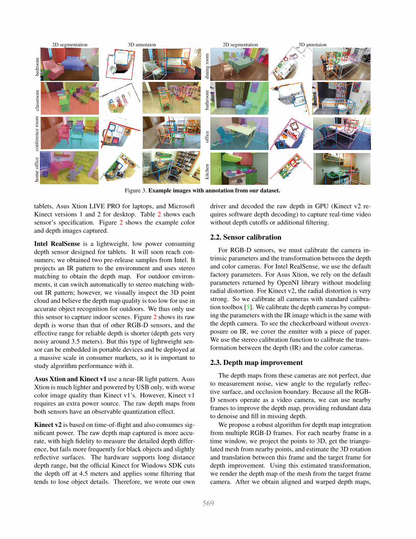
Figure 3. Example images with annotation from our dataset.

tablets, Asus Xtion LIVE PRO for laptops, and MicrosoftKinect versions 1 and 2 for desktop. Table 2 shows eachsensor’s specification. Figure 2 shows the example colorand depth images captured.

Intel RealSense is a lightweight, low power consumingdepth sensor designed for tablets. It will soon reach con-sumers; we obtained two pre-release samples from Intel. Itprojects an IR pattern to the environment and uses stereomatching to obtain the depth map. For outdoor environ-ments, it can switch automatically to stereo matching with-out IR pattern; however, we visually inspect the 3D pointcloud and believe the depth map quality is too low for use inaccurate object recognition for outdoors. We thus only usethis sensor to capture indoor scenes. Figure 2 shows its rawdepth is worse than that of other RGB-D sensors, and theeffective range for reliable depth is shorter (depth gets verynoisy around 3.5 meters). But this type of lightweight sen-sor can be embedded in portable devices and be deployed ata massive scale in consumer markets, so it is important tostudy algorithm performance with it.

Asus Xtion and Kinect v1 use a near-IR light pattern. AsusXtion is much lighter and powered by USB only, with worsecolor image quality than Kinect v1’s. However, Kinect v1requires an extra power source. The raw depth maps fromboth sensors have an observable quantization effect.

Kinect v2 is based on time-of-flight and also consumes sig-nificant power. The raw depth map captured is more accu-rate, with high fidelity to measure the detailed depth differ-ence, but fails more frequently for black objects and slightlyreflective surfaces. The hardware supports long distancedepth range, but the official Kinect for Windows SDK cutsthe depth off at 4.5 meters and applies some filtering thattends to lose object details. Therefore, we wrote our own

driver and decoded the raw depth in GPU (Kinect v2 re-quires software depth decoding) to capture real-time videowithout depth cutoffs or additional filtering.

2.2. Sensor calibration

For RGB-D sensors, we must calibrate the camera in-trinsic parameters and the transformation between the depthand color cameras. For Intel RealSense, we use the defaultfactory parameters. For Asus Xtion, we rely on the defaultparameters returned by OpenNI library without modelingradial distortion. For Kinect v2, the radial distortion is verystrong. So we calibrate all cameras with standard calibra-tion toolbox [5]. We calibrate the depth cameras by comput-ing the parameters with the IR image which is the same withthe depth camera. To see the checkerboard without overex-posure on IR, we cover the emitter with a piece of paper.We use the stereo calibration function to calibrate the trans-formation between the depth (IR) and the color cameras.

2.3. Depth map improvement

The depth maps from these cameras are not perfect, dueto measurement noise, view angle to the regularly reflec-tive surface, and occlusion boundary. Because all the RGB-D sensors operate as a video camera, we can use nearbyframes to improve the depth map, providing redundant datato denoise and fill in missing depth.

We propose a robust algorithm for depth map integrationfrom multiple RGB-D frames. For each nearby frame in atime window, we project the points to 3D, get the triangu-lated mesh from nearby points, and estimate the 3D rotationand translation between this frame and the target frame fordepth improvement. Using this estimated transformation,we render the depth map of the mesh from the target framecamera. After we obtain aligned and warped depth maps,

bathroom(6.4%)

others(8.0%)

classroom(9.3%)

office(11.0%)

furniture store(11.3%)

bedroom(12.6%)computer room(1.0%)lecture theatre(1.2%)

library(1.4%)study space(1.9%)home office(1.9%)

discussion area(2.0%)

dining area(2.4%)conference room(2.6%)

lab(3.0%)corridor(3.8%)kitchen(5.6%)

living room(6.0%)rest space(6.3%)

dining room(2.3%)

0

1250

2500

3750

5000

chair

ta

ble des

k

pillow so

fa bed

cabine

t box

garbag

e_bin

lamp

shelf

mon

itor

sofa

chair

drawer

frame

sink

paper

trash

can

side t

able

book

door

nigh

t stan

d

book s

helf

keyb

oard

compute

r to

ilet

dresse

r ra

ck

curta

in cp

u bag

cu

p tv

kitch

en ca

binet

fridge

whit

e boa

rd bott

le

printer

coffe

e tab

le

dining t

able

stoo

l

unkn

own

towel plan

t

paintin

g

compute

r mon

itor

mirro

r

hang

ing ca

binet

laptop

bow

l

board tra

y ov

en

stee

l cab

inet

bench

chair

s

mou

se

cloth

es

kitch

en

carto

n box

telep

hone

portrai

t

bathtub

Kinect v2 SUN3D (ASUS Xtion) NYUv2 (Kinect v1)

B3DO (Kinect v1)Intel RealSense

(a) object distribution (b) scene distribution19959

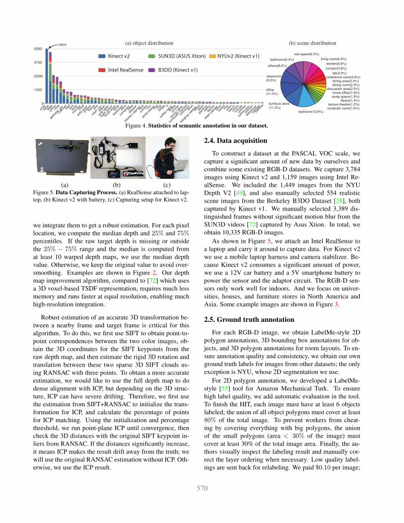
Figure 4. Statistics of semantic annotation in our dataset.

(a) (b) (c)Figure 5. Data Capturing Process. (a) RealSense attached to lap-top, (b) Kinect v2 with battery, (c) Capturing setup for Kinect v2.

we integrate them to get a robust estimation. For each pixellocation, we compute the median depth and 25% and 75%percentiles. If the raw target depth is missing or outsidethe 25% − 75% range and the median is computed fromat least 10 warped depth maps, we use the median depthvalue. Otherwise, we keep the original value to avoid over-smoothing. Examples are shown in Figure 2. Our depthmap improvement algorithm, compared to [72] which usesa 3D voxel-based TSDF representation, requires much lessmemory and runs faster at equal resolution, enabling muchhigh-resolution integration.

Robust estimation of an accurate 3D transformation be-tween a nearby frame and target frame is critical for thisalgorithm. To do this, we first use SIFT to obtain point-to-point correspondences between the two color images, ob-tain the 3D coordinates for the SIFT keypoints from theraw depth map, and then estimate the rigid 3D rotation andtranslation between these two sparse 3D SIFT clouds us-ing RANSAC with three points. To obtain a more accurateestimation, we would like to use the full depth map to dodense alignment with ICP, but depending on the 3D struc-ture, ICP can have severe drifting. Therefore, we first usethe estimation from SIFT+RANSAC to initialize the trans-formation for ICP, and calculate the percentage of pointsfor ICP matching. Using the initialization and percentagethreshold, we run point-plane ICP until convergence, thencheck the 3D distances with the original SIFT keypoint in-liers from RANSAC. If the distances significantly increase,it means ICP makes the result drift away from the truth; wewill use the original RANSAC estimation without ICP. Oth-erwise, we use the ICP result.

2.4. Data acquisition

To construct a dataset at the PASCAL VOC scale, wecapture a significant amount of new data by ourselves andcombine some existing RGB-D datasets. We capture 3,784images using Kinect v2 and 1,159 images using Intel Re-alSense. We included the 1,449 images from the NYUDepth V2 [49], and also manually selected 554 realisticscene images from the Berkeley B3DO Dataset [28], bothcaptured by Kinect v1. We manually selected 3,389 dis-tinguished frames without significant motion blur from theSUN3D videos [72] captured by Asus Xtion. In total, weobtain 10,335 RGB-D images.

As shown in Figure 5, we attach an Intel RealSense toa laptop and carry it around to capture data. For Kinect v2we use a mobile laptop harness and camera stabilizer. Be-cause Kinect v2 consumes a significant amount of power,we use a 12V car battery and a 5V smartphone battery topower the sensor and the adaptor circuit. The RGB-D sen-sors only work well for indoors. And we focus on univer-sities, houses, and furniture stores in North America andAsia. Some example images are shown in Figure 3.

2.5. Ground truth annotation

For each RGB-D image, we obtain LabelMe-style 2Dpolygon annotations, 3D bounding box annotations for ob-jects, and 3D polygon annotations for room layouts. To en-sure annotation quality and consistency, we obtain our ownground truth labels for images from other datasets; the onlyexception is NYU, whose 2D segmentation we use.

For 2D polygon annotation, we developed a LabelMe-style [55] tool for Amazon Mechanical Turk. To ensurehigh label quality, we add automatic evaluation in the tool.To finish the HIT, each image must have at least 6 objectslabeled; the union of all object polygons must cover at least80% of the total image. To prevent workers from cheat-ing by covering everything with big polygons, the unionof the small polygons (area < 30% of the image) mustcover at least 30% of the total image area. Finally, the au-thors visually inspect the labeling result and manually cor-rect the layer ordering when necessary. Low quality label-ings are sent back for relabeling. We paid $0.10 per image;

RGB (19.7) D (20.1) RGB-D (23.0) RGB (35.6) D (25.5) RGB-D (37.2) RGB (38.1) D (27.7) RGB-D (39.0)bathroombedroom

classroomcomputer room

conference roomcorridor

dining areadining room

discussion areafurniture store

home o�cekitchen

lablecture theatre

libraryliving room

o�cerest space

study space

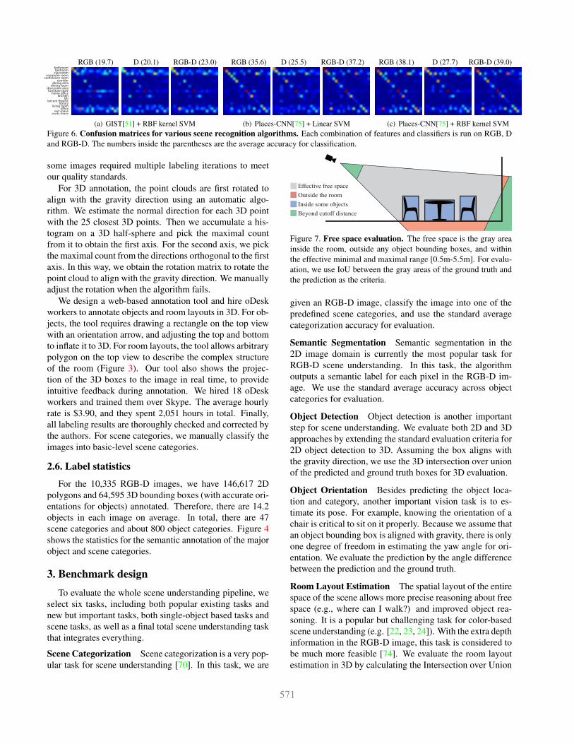
(a) GIST[51] + RBF kernel SVM (b) Places-CNN[75] + Linear SVM (c) Places-CNN[75] + RBF kernel SVMFigure 6. Confusion matrices for various scene recognition algorithms. Each combination of features and classifiers is run on RGB, Dand RGB-D. The numbers inside the parentheses are the average accuracy for classification.

some images required multiple labeling iterations to meetour quality standards.

For 3D annotation, the point clouds are first rotated toalign with the gravity direction using an automatic algo-rithm. We estimate the normal direction for each 3D pointwith the 25 closest 3D points. Then we accumulate a his-togram on a 3D half-sphere and pick the maximal countfrom it to obtain the first axis. For the second axis, we pickthe maximal count from the directions orthogonal to the firstaxis. In this way, we obtain the rotation matrix to rotate thepoint cloud to align with the gravity direction. We manuallyadjust the rotation when the algorithm fails.

We design a web-based annotation tool and hire oDeskworkers to annotate objects and room layouts in 3D. For ob-jects, the tool requires drawing a rectangle on the top viewwith an orientation arrow, and adjusting the top and bottomto inflate it to 3D. For room layouts, the tool allows arbitrarypolygon on the top view to describe the complex structureof the room (Figure 3). Our tool also shows the projec-tion of the 3D boxes to the image in real time, to provideintuitive feedback during annotation. We hired 18 oDeskworkers and trained them over Skype. The average hourlyrate is $3.90, and they spent 2,051 hours in total. Finally,all labeling results are thoroughly checked and corrected bythe authors. For scene categories, we manually classify theimages into basic-level scene categories.

2.6. Label statistics

For the 10,335 RGB-D images, we have 146,617 2Dpolygons and 64,595 3D bounding boxes (with accurate ori-entations for objects) annotated. Therefore, there are 14.2objects in each image on average. In total, there are 47scene categories and about 800 object categories. Figure 4shows the statistics for the semantic annotation of the majorobject and scene categories.

3. Benchmark designTo evaluate the whole scene understanding pipeline, we

select six tasks, including both popular existing tasks andnew but important tasks, both single-object based tasks andscene tasks, as well as a final total scene understanding taskthat integrates everything.

Scene Categorization Scene categorization is a very pop-ular task for scene understanding [70]. In this task, we are

Effective free spaceOutside the roomInside some objectsBeyond cutoff distance

Figure 7. Free space evaluation. The free space is the gray areainside the room, outside any object bounding boxes, and withinthe effective minimal and maximal range [0.5m-5.5m]. For evalu-ation, we use IoU between the gray areas of the ground truth andthe prediction as the criteria.

given an RGB-D image, classify the image into one of thepredefined scene categories, and use the standard averagecategorization accuracy for evaluation.

Semantic Segmentation Semantic segmentation in the2D image domain is currently the most popular task forRGB-D scene understanding. In this task, the algorithmoutputs a semantic label for each pixel in the RGB-D im-age. We use the standard average accuracy across objectcategories for evaluation.

Object Detection Object detection is another importantstep for scene understanding. We evaluate both 2D and 3Dapproaches by extending the standard evaluation criteria for2D object detection to 3D. Assuming the box aligns withthe gravity direction, we use the 3D intersection over unionof the predicted and ground truth boxes for 3D evaluation.

Object Orientation Besides predicting the object loca-tion and category, another important vision task is to es-timate its pose. For example, knowing the orientation of achair is critical to sit on it properly. Because we assume thatan object bounding box is aligned with gravity, there is onlyone degree of freedom in estimating the yaw angle for ori-entation. We evaluate the prediction by the angle differencebetween the prediction and the ground truth.

Room Layout Estimation The spatial layout of the entirespace of the scene allows more precise reasoning about freespace (e.g., where can I walk?) and improved object rea-soning. It is a popular but challenging task for color-basedscene understanding (e.g. [22, 23, 24]). With the extra depthinformation in the RGB-D image, this task is considered tobe much more feasible [74]. We evaluate the room layoutestimation in 3D by calculating the Intersection over Union

meanRGB NN 45.03 27.89 16.89 18.51 21.77 1.06 4.07 0 8.32Depth NN 42.6 9.65 21.51 12.47 6.44 2.55 0.6 0.3 5.32

RGB-D NN 45.78 35.75 19.86 19.29 23.3 1.66 6.09 0.7 8.97RGB [40] 47.22 39.14 17.21 20.43 21.53 1.49 5.94 0 9.33Depth [40] 43.83 13.9 22.31 12.88 6.3 1.49 0.45 0.25 5.98

RGB-D [40] 48.25 49.18 20.8 20.92 23.61 1.83 8.73 0.77 10.05RGB-D [53] 78.64 84.51 33.15 34.25 42.52 25.01 35.74 35.71 36.33

Table 3. Semantic segmentation. We evaluate performance for 40object categories. Here shows 8 selected ones: floor, ceiling, chair,table, bed, nightstand, books, and person. The mean accuracy isfor all the 40 categories. A full table is in the supp. material.

mAPSliding Shapes [62] 33.42 25.78 42.09 61.86 23.28 37.29

Table 4. 3D object detection.

(IoU) between the free space from the ground truth and thefree space predicted by the algorithm output.

As shown in Figure 7, the free space is defined as thespace that satisfies four conditions: 1) within camera fieldof view, 2) within effective range, 3) within the room, and4) outside any object bounding box (for room layout esti-mation, we assume empty rooms without objects). In termsof implementation, we define a voxel grid of 0.1×0.1×0.1meter3 over the space and choose the voxels that are insidethe field of view of the camera and fall between 0.5 and 5.5meters from the camera, which is an effective range for mostRGB-D sensors. For each of these effective voxels, given aroom layout 3D polygon, we check whether the voxel is in-side. In this way, we can compute the intersection and theunion by counting 3D voxels.

This evaluation metric directly measures the free spaceprediction accuracy. However, we care only about the spacewithin a 5.5 meter range; if a room is too big, all effectivevoxels will be in the ground truth room. If an algorithm pre-dicts a huge room beyond 5.5 meters, then the IoU will beequal to one, which introduces bias: algorithms will favora huge room. To address this issue, we only evaluate algo-rithms on the rooms with reasonable size (not too big), sincenone of the RGB-D sensors can see very far either. If thepercentage of effective 3D voxels in the ground truth roomis bigger than 95%, we discard the room in our evaluation.

Total Scene Understanding The final task for our sceneunderstanding benchmark is to estimate the whole scene in-cluding objects and room layout in 3D [38]. This task is alsoreferred to “Basic Level Scene Understanding” in [71]. Wepropose this benchmark task as the final goal to integrateboth object detection and room layout estimation to obtaina total scene understanding, recognizing and localizing allthe objects and the room structure.

We evaluate the result by comparing the ground truth ob-jects and the predicted objects. To match the prediction withground truth, we compute the IoU between all pairs of pre-

Angle: 12.6 IoU: 0.7 Angle: 87.4 IoU: 0.4 Angle: 31.4 IoU: 0.24

Angle: 8.6 IoU: 0.7Angle: 3.54 IoU: 0.66

Angle: 49.5 IoU: 0.6

Angle: 1.6 IoU: 0.6 Angle: 2.4 IoU: 0.7

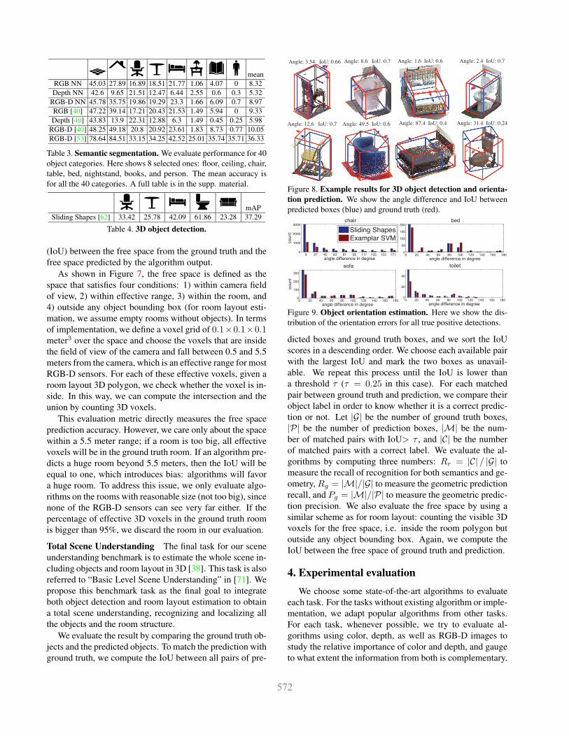
Figure 8. Example results for 3D object detection and orienta-tion prediction. We show the angle difference and IoU betweenpredicted boxes (blue) and ground truth (red).

0 20 40 60 80 100 120 140 160 1800

100

200

300

angle difference in degree

coun

t

sofa

9 27 45 63 81 99 117 135 153 1710

1000

2000

3000

angle difference in degree

coun

t

chair

Sliding ShapesExamplar SVM

0 20 40 60 80 100 120 140 160 1800

20

40

angle difference in degree

toilet

0 20 40 60 80 100 120 140 160 1800

50

100

150

200

angle difference in degree

bed

Figure 9. Object orientation estimation. Here we show the dis-tribution of the orientation errors for all true positive detections.

dicted boxes and ground truth boxes, and we sort the IoUscores in a descending order. We choose each available pairwith the largest IoU and mark the two boxes as unavail-able. We repeat this process until the IoU is lower thana threshold τ (τ = 0.25 in this case). For each matchedpair between ground truth and prediction, we compare theirobject label in order to know whether it is a correct predic-tion or not. Let |G| be the number of ground truth boxes,|P| be the number of prediction boxes, |M| be the num-ber of matched pairs with IoU> τ , and |C| be the numberof matched pairs with a correct label. We evaluate the al-gorithms by computing three numbers: Rr = |C| / |G| tomeasure the recall of recognition for both semantics and ge-ometry, Rg = |M|/|G| to measure the geometric predictionrecall, and Pg = |M|/|P| to measure the geometric predic-tion precision. We also evaluate the free space by using asimilar scheme as for room layout: counting the visible 3Dvoxels for the free space, i.e. inside the room polygon butoutside any object bounding box. Again, we compute theIoU between the free space of ground truth and prediction.

4. Experimental evaluationWe choose some state-of-the-art algorithms to evaluate

each task. For the tasks without existing algorithm or imple-mentation, we adapt popular algorithms from other tasks.For each task, whenever possible, we try to evaluate al-gorithms using color, depth, as well as RGB-D images tostudy the relative importance of color and depth, and gaugeto what extent the information from both is complementary.

mAPRGB-D ESVM 7.38 12.95 7.44 0.09 12.47 0.02 0.86 0.57 1.87 6.01 6.12 0.41 6.00 1.61 6.19 14.02 11.89 0.75 14.79 5.86RGB-D DPM 34.23 54.74 14.40 0.45 29.30 0.87 4.75 0.43 1.82 13.25 23.38 11.99 23.39 9.36 15.59 21.62 24.04 8.73 23.79 16.64

RGB-D RCNN[20] 49.56 75.97 34.99 5.78 41.22 8.08 16.55 4.17 31.38 46.83 21.98 10.77 37.17 16.5 41.92 42.2 43.02 32.92 69.84 35.20Table 5. Evaluation of 2D object detection. We evaluate on 19 popular object categories using Average Precision (AP): bathtub, bed,bookshelf, box, chair, counter, desk, door, dresser, garbage bin, lamp, monitor, night stand, pillow, sink, sofa, table, tv and toilet.

Manhattan Box (0.99)Ground Truth Geometric Context (0.27)Convex Hull (0.90)

Convex Hull (0.85)

Geometric Context (0.61)Convex Hull (0.43)Manhattan Box (0.72)

Geometric Context (0.57)Ground Truth

Ground Truth

Manhattan Box (0.811)

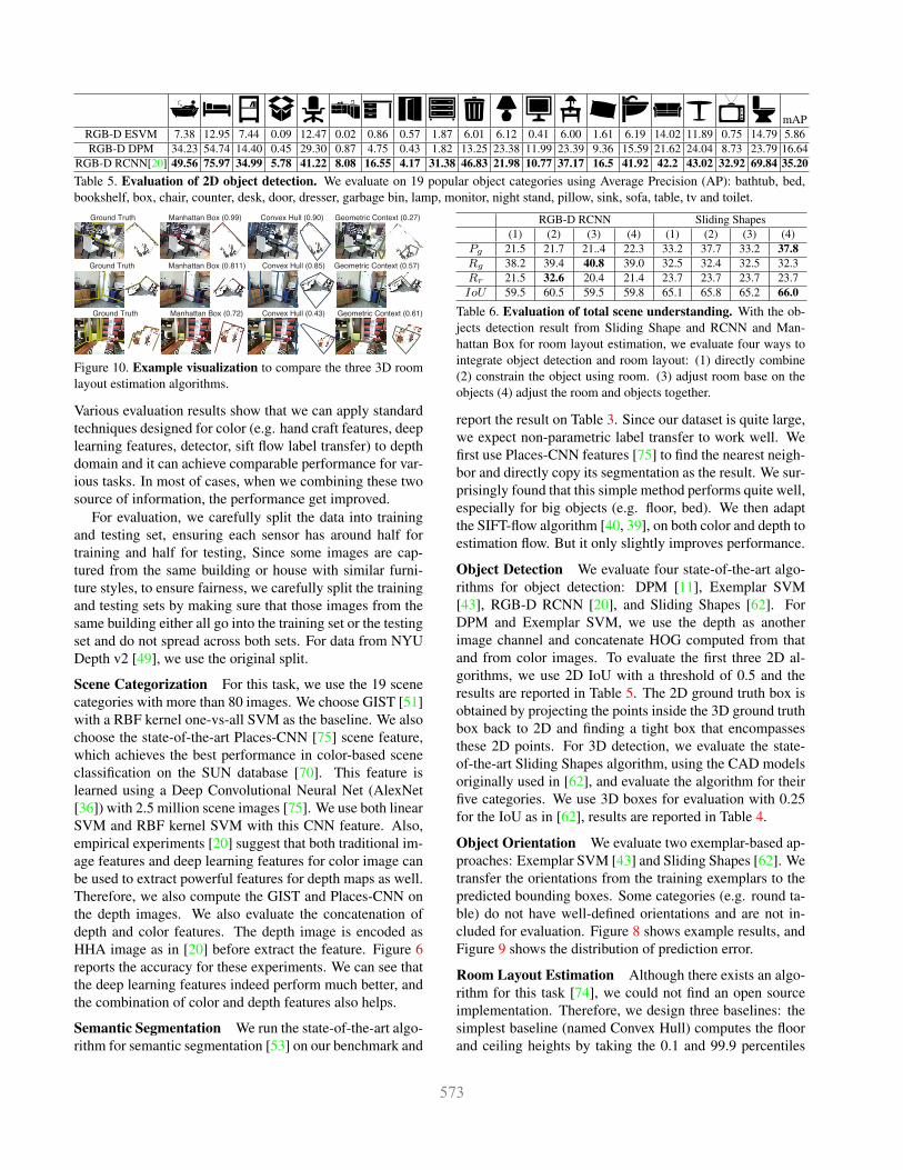
Figure 10. Example visualization to compare the three 3D roomlayout estimation algorithms.

Various evaluation results show that we can apply standardtechniques designed for color (e.g. hand craft features, deeplearning features, detector, sift flow label transfer) to depthdomain and it can achieve comparable performance for var-ious tasks. In most of cases, when we combining these twosource of information, the performance get improved.

For evaluation, we carefully split the data into trainingand testing set, ensuring each sensor has around half fortraining and half for testing, Since some images are cap-tured from the same building or house with similar furni-ture styles, to ensure fairness, we carefully split the trainingand testing sets by making sure that those images from thesame building either all go into the training set or the testingset and do not spread across both sets. For data from NYUDepth v2 [49], we use the original split.

Scene Categorization For this task, we use the 19 scenecategories with more than 80 images. We choose GIST [51]with a RBF kernel one-vs-all SVM as the baseline. We alsochoose the state-of-the-art Places-CNN [75] scene feature,which achieves the best performance in color-based sceneclassification on the SUN database [70]. This feature islearned using a Deep Convolutional Neural Net (AlexNet[36]) with 2.5 million scene images [75]. We use both linearSVM and RBF kernel SVM with this CNN feature. Also,empirical experiments [20] suggest that both traditional im-age features and deep learning features for color image canbe used to extract powerful features for depth maps as well.Therefore, we also compute the GIST and Places-CNN onthe depth images. We also evaluate the concatenation ofdepth and color features. The depth image is encoded asHHA image as in [20] before extract the feature. Figure 6reports the accuracy for these experiments. We can see thatthe deep learning features indeed perform much better, andthe combination of color and depth features also helps.

Semantic Segmentation We run the state-of-the-art algo-rithm for semantic segmentation [53] on our benchmark and

RGB-D RCNN Sliding Shapes(1) (2) (3) (4) (1) (2) (3) (4)

Pg 21.5 21.7 21..4 22.3 33.2 37.7 33.2 37.8Rg 38.2 39.4 40.8 39.0 32.5 32.4 32.5 32.3Rr 21.5 32.6 20.4 21.4 23.7 23.7 23.7 23.7IoU 59.5 60.5 59.5 59.8 65.1 65.8 65.2 66.0

Table 6. Evaluation of total scene understanding. With the ob-jects detection result from Sliding Shape and RCNN and Man-hattan Box for room layout estimation, we evaluate four ways tointegrate object detection and room layout: (1) directly combine(2) constrain the object using room. (3) adjust room base on theobjects (4) adjust the room and objects together.

report the result on Table 3. Since our dataset is quite large,we expect non-parametric label transfer to work well. Wefirst use Places-CNN features [75] to find the nearest neigh-bor and directly copy its segmentation as the result. We sur-prisingly found that this simple method performs quite well,especially for big objects (e.g. floor, bed). We then adaptthe SIFT-flow algorithm [40, 39], on both color and depth toestimation flow. But it only slightly improves performance.

Object Detection We evaluate four state-of-the-art algo-rithms for object detection: DPM [11], Exemplar SVM[43], RGB-D RCNN [20], and Sliding Shapes [62]. ForDPM and Exemplar SVM, we use the depth as anotherimage channel and concatenate HOG computed from thatand from color images. To evaluate the first three 2D al-gorithms, we use 2D IoU with a threshold of 0.5 and theresults are reported in Table 5. The 2D ground truth box isobtained by projecting the points inside the 3D ground truthbox back to 2D and finding a tight box that encompassesthese 2D points. For 3D detection, we evaluate the state-of-the-art Sliding Shapes algorithm, using the CAD modelsoriginally used in [62], and evaluate the algorithm for theirfive categories. We use 3D boxes for evaluation with 0.25for the IoU as in [62], results are reported in Table 4.

Object Orientation We evaluate two exemplar-based ap-proaches: Exemplar SVM [43] and Sliding Shapes [62]. Wetransfer the orientations from the training exemplars to thepredicted bounding boxes. Some categories (e.g. round ta-ble) do not have well-defined orientations and are not in-cluded for evaluation. Figure 8 shows example results, andFigure 9 shows the distribution of prediction error.

Room Layout Estimation Although there exists an algo-rithm for this task [74], we could not find an open sourceimplementation. Therefore, we design three baselines: thesimplest baseline (named Convex Hull) computes the floorand ceiling heights by taking the 0.1 and 99.9 percentiles

IoU 50.7 Rr: 0.333 Rg: 0.333 Pg : 0.375IoU: 53.1 Rr: 0.333 Rg: 0.333 Pg: 0.125 IoU: 57.3 Rr :0.33 Rg: 0.667 Pg:0.125

IoU: 53.1 Rr: 0.111 Rg : 0.111 Pg: 0.5IoU 72.9 Rr: 0.333 Rg: 0.667 Pg: 0.667 IoU 63.9 Rr: 0.333 Rg: 0.667 Pg:1IoU: 77.0 Rr: 0.25 Rg: 0.25 Pg: 0.5

IoU: 78.8 Rr: 1 Rg: 1 Pg: 0.5

Gro

und

truth

Slid

ing

Shap

es3D

RC

NN

IoU: 54.6 Rr : 0.333 Rg : 0.333 Pg: 0.125

IoU:60 Rr: 0.50 Rg : 0.0.50 Pg: 0.5

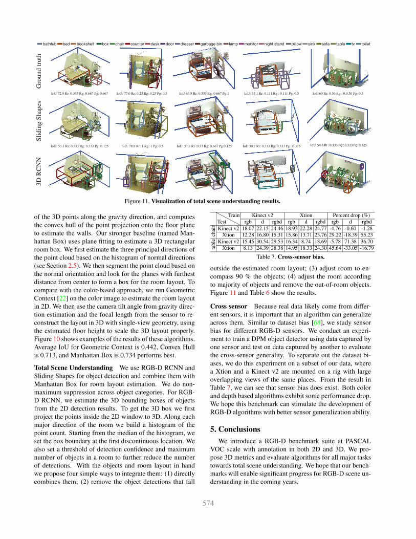
bathtub bed bookshelf box chair counter desk door dresser garbage bin lamp monitor night stand pillow sink sofa table tv toilet

Figure 11. Visualization of total scene understanding results.

of the 3D points along the gravity direction, and computesthe convex hull of the point projection onto the floor planeto estimate the walls. Our stronger baseline (named Man-hattan Box) uses plane fitting to estimate a 3D rectangularroom box. We first estimate the three principal directions ofthe point cloud based on the histogram of normal directions(see Section 2.5). We then segment the point cloud based onthe normal orientation and look for the planes with furthestdistance from center to form a box for the room layout. Tocompare with the color-based approach, we run GeometricContext [22] on the color image to estimate the room layoutin 2D. We then use the camera tilt angle from gravity direc-tion estimation and the focal length from the sensor to re-construct the layout in 3D with single-view geometry, usingthe estimated floor height to scale the 3D layout properly.Figure 10 shows examples of the results of these algorithms.Average IoU for Geometric Context is 0.442, Convex Hullis 0.713, and Manhattan Box is 0.734 performs best.

Total Scene Understanding We use RGB-D RCNN andSliding Shapes for object detection and combine them withManhattan Box for room layout estimation. We do non-maximum suppression across object categories. For RGB-D RCNN, we estimate the 3D bounding boxes of objectsfrom the 2D detection results. To get the 3D box we firstproject the points inside the 2D window to 3D. Along eachmajor direction of the room we build a histogram of thepoint count. Starting from the median of the histogram, weset the box boundary at the first discontinuous location. Wealso set a threshold of detection confidence and maximumnumber of objects in a room to further reduce the numberof detections. With the objects and room layout in handwe propose four simple ways to integrate them: (1) directlycombines them; (2) remove the object detections that fall

TestTrain Kinect v2 Xtion Percent drop (%)

rgb d rgbd rgb d rgbd rgb d rgbd

chai

r Kinect v2 18.07 22.15 24.46 18.93 22.28 24.77 -4.76 -0.60 -1.28Xtion 12.28 16.80 15.31 15.86 13.71 23.76 29.22 -18.39 55.23

tabl

e Kinect v2 15.45 30.54 29.53 16.34 8.74 18.69 -5.78 71.38 36.70Xtion 8.13 24.39 28.38 14.95 18.33 24.30 45.64 -33.05 -16.79

Table 7. Cross-sensor bias.

outside the estimated room layout; (3) adjust room to en-compass 90 % the objects; (4) adjust the room accordingto majority of objects and remove the out-of-room objects.Figure 11 and Table 6 show the results.

Cross sensor Because real data likely come from differ-ent sensors, it is important that an algorithm can generalizeacross them. Similar to dataset bias [68], we study sensorbias for different RGB-D sensors. We conduct an experi-ment to train a DPM object detector using data captured byone sensor and test on data captured by another to evaluatethe cross-sensor generality. To separate out the dataset bi-ases, we do this experiment on a subset of our data, wherea Xtion and a Kinect v2 are mounted on a rig with largeoverlapping views of the same places. From the result inTable 7, we can see that sensor bias does exist. Both colorand depth based algorithms exhibit some performance drop.We hope this benchmark can stimulate the development ofRGB-D algorithms with better sensor generalization ability.

5. ConclusionsWe introduce a RGB-D benchmark suite at PASCAL

VOC scale with annotation in both 2D and 3D. We pro-pose 3D metrics and evaluate algorithms for all major taskstowards total scene understanding. We hope that our bench-marks will enable significant progress for RGB-D scene un-derstanding in the coming years.

Acknowledgement. This work is supported by gift fundsfrom Intel Corporation. We thank Thomas Funkhouser, Ji-tendra Malik, Alexi A. Efros and Szymon Rusinkiewicz forvaluable discussion. We also thank Linguang Zhang, FisherYu, Yinda Zhang, Luna Song, Zhirong Wu, Pingmei Xu,Guoxuan Zhang and others for data capturing and labeling.

References[1] A. Aldoma, F. Tombari, L. Di Stefano, and M. Vincze. A

global hypotheses verification method for 3d object recogni-tion. In ECCV. 2012. 2

[2] A. Anand, H. S. Koppula, T. Joachims, and A. Saxena.Contextually guided semantic labeling and search for three-dimensional point clouds. IJRR, 2012. 2

[3] B. I. Barbosa, M. Cristani, A. Del Bue, L. Bazzani, andV. Murino. Re-identification with rgb-d sensors. In FirstInternational Workshop on Re-Identification, 2012. 2

[4] J. T. Barron and J. Malik. Intrinsic scene properties from asingle rgb-d image. CVPR, 2013. 1

[5] J.-Y. Bouguet. Camera calibration toolbox for matlab. 2004.3

[6] C. S. Catalin Ionescu, Fuxin Li. Latent structured models forhuman pose estimation. In ICCV, 2011. 2

[7] J. Deng, W. Dong, R. Socher, L.-J. Li, K. Li, and L. Fei-Fei. Imagenet: A large-scale hierarchical image database. InCVPR, 2009. 2

[8] N. Erdogmus and S. Marcel. Spoofing in 2d face recognitionwith 3d masks and anti-spoofing with kinect. In BTAS, 2013.2

[9] M. Everingham, L. Van Gool, C. K. I. Williams, J. Winn,and A. Zisserman. The pascal visual object classes (voc)challenge. IJCV, 2010. 1, 2

[10] G. Fanelli, M. Dantone, J. Gall, A. Fossati, and L. Van Gool.Random forests for real time 3d face analysis. IJCV, 2013. 2

[11] P. F. Felzenszwalb, R. B. Girshick, D. McAllester, and D. Ra-manan. Object detection with discriminatively trained partbased models. PAMI, 2010. 7

[12] S. Fothergill, H. M. Mentis, P. Kohli, and S. Nowozin. In-structing people for training gestural interactive systems. InCHI, 2012. 2

[13] D. F. Fouhey, A. Gupta, and M. Hebert. Data-driven 3d prim-itives for single image understanding. In ICCV, 2013. 2

[14] D. F. Fouhey, A. Gupta, and M. Hebert. Unfolding an indoororigami world. In ECCV. 2014. 2

[15] R. Girshick, J. Donahue, T. Darrell, and J. Malik. Rich fea-ture hierarchies for accurate object detection and semanticsegmentation. In CVPR, 2014. 1

[16] D. Gossow, D. Weikersdorfer, and M. Beetz. Distinctive tex-ture features from perspective-invariant keypoints. In ICPR,2012. 2

[17] R. Guo and D. Hoiem. Support surface prediction in indoorscenes. In ICCV, 2013. 1

[18] R. Guo and D. Hoiem. Support surface prediction in indoorscenes. In ICCV, 2013. 2

[19] S. Gupta, P. Arbelaez, and J. Malik. Perceptual organizationand recognition of indoor scenes from RGB-D images. InCVPR, 2013. 1, 2

[20] S. Gupta, R. Girshick, P. Arbelaez, and J. Malik. Learningrich features from RGB-D images for object detection andsegmentation. In ECCV, 2014. 1, 2, 7

[21] A. Handa, T. Whelan, J. McDonald, and A. Davison. Abenchmark for RGB-D visual odometry, 3D reconstructionand SLAM. In ICRA, 2014. 2

[22] V. Hedau, D. Hoiem, and D. Forsyth. Recovering the spatiallayout of cluttered rooms. In ICCV, 2009. 5, 8

[23] V. Hedau, D. Hoiem, and D. Forsyth. Thinking inside thebox: Using appearance models and context based on roomgeometry. In ECCV. 2010. 5

[24] V. Hedau, D. Hoiem, and D. Forsyth. Recovering free spaceof indoor scenes from a single image. In CVPR, 2012. 5

[25] S. Hinterstoisser, V. Lepetit, S. Ilic, S. Holzer, G. Bradski,K. Konolige, and N. Navab. Model based training, detec-tion and pose estimation of texture-less 3d objects in heavilycluttered scenes. In ACCV. 2013. 2

[26] C. Ionescu, D. Papava, V. Olaru, and C. Sminchisescu. Hu-man3.6m: Large scale datasets and predictive methods for3d human sensing in natural environments. PAMI, 2014. 2

[27] S. Izadi, D. Kim, O. Hilliges, D. Molyneaux, R. Newcombe,P. Kohli, J. Shotton, S. Hodges, D. Freeman, A. Davison, andA. Fitzgibbon. Kinectfusion: Real-time 3d reconstructionand interaction using a moving depth camera. In UIST, 2011.1

[28] A. Janoch, S. Karayev, Y. Jia, J. T. Barron, M. Fritz,K. Saenko, and T. Darrell. A category-level 3-d objectdataset: Putting the kinect to work. In ICCV Workshop onConsumer Depth Cameras for Computer Vision, 2011. 2, 4

[29] A. Janoch, S. Karayev, Y. Jia, J. T. Barron, M. Fritz,K. Saenko, and T. Darrell. A category-level 3d object dataset:Putting the kinect to work. 2013. 2

[30] Z. Jia, A. Gallagher, A. Saxena, and T. Chen. 3d-based rea-soning with blocks, support, and stability. In CVPR, 2013.1

[31] H. Jiang. Finding approximate convex shapes in rgbd im-ages. In ECCV. 2014. 2

[32] H. Jiang and J. Xiao. A linear approach to matching cuboidsin RGBD images. In CVPR, 2013. 1, 2

[33] M. Kepski and B. Kwolek. Fall detection using ceiling-mounted 3d depth camera. 2

[34] H. S. Koppula, A. Anand, T. Joachims, and A. Saxena. Se-mantic labeling of 3d point clouds for indoor scenes. InNIPS, 2011. 2

[35] H. S. Koppula, R. Gupta, and A. Saxena. Learning humanactivities and object affordances from rgb-d videos. IJRR,2013. 2

[36] A. Krizhevsky, I. Sutskever, and G. E. Hinton. Imagenetclassification with deep convolutional neural networks. InNIPS, 2012. 1, 7

[37] K. Lai, L. Bo, X. Ren, and D. Fox. A large-scale hierarchicalmulti-view rgb-d object dataset. In ICRA, 2011. 2

[38] D. Lin, S. Fidler, and R. Urtasun. Holistic scene understand-ing for 3d object detection with RGBD cameras. In ICCV,2013. 1, 2, 6

[39] C. Liu, J. Yuen, and A. Torralba. Nonparametric scene pars-ing: Label transfer via dense scene alignment. In CVPR,2009. 7

[40] C. Liu, J. Yuen, and A. Torralba. Sift flow: Dense corre-spondence across scenes and its applications. PAMI, 2011.6, 7

[41] L. Liu and L. Shao. Learning discriminative representationsfrom rgb-d video data. In IJCAI, 2013. 2

[42] M. Luber, L. Spinello, and K. O. Arras. People trackingin rgb-d data with on-line boosted target models. In IROS,2011. 2

[43] T. Malisiewicz, A. Gupta, and A. A. Efros. Ensemble ofexemplar-svms for object detection and beyond. In ICCV,2011. 7

[44] J. Mason, B. Marthi, and R. Parr. Object disappearance forobject discovery. In IROS, 2012. 2

[45] O. Mattausch, D. Panozzo, C. Mura, O. Sorkine-Hornung,and R. Pajarola. Object detection and classification fromlarge-scale cluttered indoor scans. In Computer GraphicsForum, 2014. 2

[46] S. Meister, S. Izadi, P. Kohli, M. Hammerle, C. Rother, andD. Kondermann. When can we use kinectfusion for groundtruth acquisition? In Proc. Workshop on Color-Depth Cam-era Fusion in Robotics, 2012. 2

[47] A. Mian, M. Bennamoun, and R. Owens. On the repeatabil-ity and quality of keypoints for local feature-based 3d objectretrieval from cluttered scenes. IJCV, 2010. 2

[48] R. Min, N. Kose, and J.-L. Dugelay. Kinectfacedb: A kinectdatabase for face recognition. 2

[49] P. K. Nathan Silberman, Derek Hoiem and R. Fergus. Indoorsegmentation and support inference from rgbd images. InECCV, 2012. 1, 2, 4, 7

[50] B. Ni, G. Wang, and P. Moulin. Rgbd-hudaact: A color-depthvideo database for human daily activity recognition. 2011. 2

[51] A. Oliva and A. Torralba. Modeling the shape of the scene:A holistic representation of the spatial envelope. IJCV, 2001.5, 7

[52] F. Pomerleau, S. Magnenat, F. Colas, M. Liu, and R. Sieg-wart. Tracking a depth camera: Parameter exploration forfast icp. In IROS, 2011. 2

[53] X. Ren, L. Bo, and D. Fox. Rgb-(d) scene labeling: Featuresand algorithms. In CVPR, 2012. 1, 2, 6, 7

[54] A. Richtsfeld, T. Morwald, J. Prankl, M. Zillich, andM. Vincze. Segmentation of unknown objects in indoor en-vironments. In IROS, 2012. 2

[55] B. C. Russell, A. Torralba, K. P. Murphy, and W. T. Freeman.Labelme: a database and web-based tool for image annota-tion. IJCV, 2008. 4

[56] J. Shotton, R. Girshick, A. Fitzgibbon, T. Sharp, M. Cook,M. Finocchio, R. Moore, P. Kohli, A. Criminisi, A. Kipman,et al. Efficient human pose estimation from single depth im-ages. PAMI, 2013. 1

[57] J. Shotton, B. Glocker, C. Zach, S. Izadi, A. Criminisi, andA. Fitzgibbon. Scene coordinate regression forests for cam-era relocalization in rgb-d images. In CVPR, 2013. 2

[58] J. Shotton, T. Sharp, A. Kipman, A. Fitzgibbon, M. Finoc-chio, A. Blake, M. Cook, and R. Moore. Real-time humanpose recognition in parts from single depth images. Commu-nications of the ACM, 2013. 1

[59] A. Shrivastava and A. Gupta. Building part-based object de-tectors via 3d geometry. In ICCV, 2013. 2

[60] N. Silberman and R. Fergus. Indoor scene segmentation us-ing a structured light sensor. In Proceedings of the Inter-national Conference on Computer Vision - Workshop on 3DRepresentation and Recognition, 2011. 2

[61] A. Singh, J. Sha, K. S. Narayan, T. Achim, and P. Abbeel.Bigbird: A large-scale 3d database of object instances. InICRA, 2014. 2

[62] S. Song and J. Xiao. Sliding Shapes for 3D object detectionin RGB-D images. In ECCV, 2014. 2, 6, 7

[63] L. Spinello and K. O. Arras. People detection in rgb-d data.In IROS, 2011. 2

[64] S. Stein and S. J. McKenna. Combining embedded ac-celerometers with computer vision for recognizing foodpreparation activities. In Proceedings of the 2013 ACM inter-national joint conference on Pervasive and ubiquitous com-puting, 2013. 2

[65] S. Stein and S. J. McKenna. User-adaptive models for rec-ognizing food preparation activities. 2013. 2

[66] J. Sturm, N. Engelhard, F. Endres, W. Burgard, and D. Cre-mers. A benchmark for the evaluation of rgb-d slam systems.In IROS, 2012. 2

[67] J. Sung, C. Ponce, B. Selman, and A. Saxena. Human ac-tivity detection from rgbd images. Plan, Activity, and IntentRecognition, 2011. 2

[68] A. Torralba and A. A. Efros. Unbiased look at dataset bias.In CVPR, 2011. 8

[69] Z. Wu, S. Song, A. Khosla, X. Tang, and J. Xiao. 3DShapeNets: A deep representation for volumetric shape mod-eling. CVPR, 2015. 2

[70] J. Xiao, J. Hays, K. A. Ehinger, A. Oliva, and A. Torralba.SUN database: Large-scale scene recognition from abbey tozoo. In CVPR, 2010. 5, 7

[71] J. Xiao, J. Hays, B. C. Russell, G. Patterson, K. Ehinger,A. Torralba, and A. Oliva. Basic level scene understanding:Categories, attributes and structures. Frontiers in Psychol-ogy, 4(506), 2013. 6

[72] J. Xiao, A. Owens, and A. Torralba. SUN3D: A databaseof big spaces reconstructed using SfM and object labels. InICCV, 2013. 1, 2, 4

[73] B. Zeisl, K. Koser, and M. Pollefeys. Automatic registrationof rgb-d scans via salient directions. In ICCV, 2013. 2

[74] J. Zhang, C. Kan, A. G. Schwing, and R. Urtasun. Estimat-ing the 3d layout of indoor scenes and its clutter from depthsensors. In ICCV, 2013. 2, 5, 7

[75] B. Zhou, J. Xiao, A. Lapedriza, A. Torralba, and A. Oliva.Learning deep features for scene recognition using placesdatabase. In NIPS, 2014. 5, 7