SANDIA REPORT SAND2014-3242 Unlimited Release April 2014

Sun-Relative Pointing for Dual-Axis Solar Trackers Employing Azimuth and Elevation Rotations

Daniel M. Riley, Clifford W. Hansen

Prepared by Sandia National Laboratories Albuquerque, New Mexico 87185 and Livermore, California 94550

Sandia National Laboratories is a multi-program laboratory managed and operated by Sandia Corporation, a wholly owned subsidiary of Lockheed Martin Corporation, for the U.S. Department of Energy's National Nuclear Security Administration under contract DE-AC04-94AL85000. Approved for public release; further dissemination unlimited.

2

Issued by Sandia National Laboratories, operated for the United States Department of Energy

by Sandia Corporation.

NOTICE: This report was prepared as an account of work sponsored by an agency of the

United States Government. Neither the United States Government, nor any agency thereof,

nor any of their employees, nor any of their contractors, subcontractors, or their employees,

make any warranty, express or implied, or assume any legal liability or responsibility for the

accuracy, completeness, or usefulness of any information, apparatus, product, or process

disclosed, or represent that its use would not infringe privately owned rights. Reference herein

to any specific commercial product, process, or service by trade name, trademark,

manufacturer, or otherwise, does not necessarily constitute or imply its endorsement,

recommendation, or favoring by the United States Government, any agency thereof, or any of

their contractors or subcontractors. The views and opinions expressed herein do not

necessarily state or reflect those of the United States Government, any agency thereof, or any

of their contractors.

Printed in the United States of America. This report has been reproduced directly from the best

available copy.

Available to DOE and DOE contractors from

U.S. Department of Energy

Office of Scientific and Technical Information

P.O. Box 62

Oak Ridge, TN 37831

Telephone: (865) 576-8401

Facsimile: (865) 576-5728

E-Mail: reports@adonis.osti.gov

Online ordering: http://www.osti.gov/bridge

Available to the public from

U.S. Department of Commerce

National Technical Information Service

5285 Port Royal Rd.

Springfield, VA 22161

Telephone: (800) 553-6847

Facsimile: (703) 605-6900

E-Mail: orders@ntis.fedworld.gov

Online order: http://www.ntis.gov/help/ordermethods.asp?loc=7-4-0#online

3

SAND2014-3242

Unlimited Release

April 2014

Sun-Relative Pointing for Dual-Axis Solar Trackers Employing Azimuth and Elevation

Rotations

Daniel M. Riley, Clifford W. Hansen

Photovoltaics and Distributed Systems Integration Department

Sandia National Laboratories

P.O. Box 5800

Albuquerque, New Mexico 87185-MS0951

Abstract

Dual axis trackers employing azimuth and elevation rotations are common in the field

of photovoltaic (PV) energy generation. Accurate sun-tracking algorithms are widely

available. However, a steering algorithm has not been available to accurately point

the tracker away from the sun such that a vector projection of the sun beam onto the

tracker face falls along a desired path relative to the tracker face. We have developed

an algorithm which produces the appropriate azimuth and elevation angles for a dual

axis tracker when given the sun position, desired angle of incidence, and the desired

projection of the sun beam onto the tracker face. Development of this algorithm was

inspired by the need to accurately steer a tracker to desired sun-relative positions in

order to better characterize the electro-optical properties of PV and CPV modules.

4

5

CONTENTS

1. Introduction ................................................................................................................................ 7 1.1. Definitions....................................................................................................................... 7

1.1.1. Sun position ...................................................................................................... 7 1.1.2. Tracker rotation ................................................................................................. 8

1.1.3. Angle of incidence and angle of incidence direction ........................................ 9

2. Calculation of variables ........................................................................................................... 11

2.1. Calculating 𝛼 and 𝛽 given sun and tracker positions ................................................... 11

2.2. Calculating tracker position given sun position, α, and β ............................................ 12

2.2.1. General case when 𝑡𝑎𝑛𝛽 is defined ................................................................ 13

2.2.2. Special case when 𝑡𝑎𝑛𝛽 is undefined ............................................................. 15

2.2.3. Special case when 𝑡𝑎𝑛𝛽 = 0 and 𝜃𝑆𝐸 = 90 ................................................... 16

3. Pitfalls when computing values numerically ........................................................................... 17 3.1. Evaluating inverse cosine and inverse sine ................................................................... 17

3.2. Comparison for equality ............................................................................................... 17

3.2. Evaluating when θ𝑆𝐸 is 0 .............................................................................................. 17

4. Conclusions .............................................................................................................................. 19

5. References ................................................................................................................................ 21

Distribution ................................................................................................................................... 23

FIGURES

Figure 1: Description of solar position angles from an observer on Earth's surface ...................... 8 Figure 2: Description of the tracker-face coordinate system in which AOI direction is defined . 10

6

NOMENCLATURE

AOI Angle of incidence

CPV Concentrating photovoltaic

DOE Department of Energy

LCPV Low concentration photovoltaic

PV Photovoltaic

SNL Sandia National Laboratories

𝜃𝑆𝐴 Sun azimuth

𝜃𝑆𝐸 Sun elevation

𝜃𝑇𝐴 Tracker azimuth rotation

𝜃𝑇𝐸 Tracker elevation rotation

𝛼 Angle of incidence, AOI

𝛽 Angle of incidence direction on tracker face

�̂� Reference unit vector for topocentric coordinate system, points east

�̂� Reference unit vector for topocentric coordinate system, points north

�̂� Reference unit vector for topocentric coordinate system, points up (toward zenith)

𝑆 Sun pointing vector expressed in topocentric coordinate system

𝑥𝑚 Unit vector in tracker plane, orthogonal to 𝑦𝑚 and 𝑧𝑚

𝑦𝑚 Unit vector normal to tracker plane, orthogonal to 𝑥𝑚 and 𝑧𝑚

𝑧𝑚 Unit vector in tracker plane towards top of tracker, orthogonal to 𝑦𝑚 and 𝑥𝑚

7

1. INTRODUCTION

Dual axis trackers are common in the photovoltaic (PV) and concentrating photovoltaic (CPV)

industries as a method of pointing at the sun to maximize solar energy collection. They are also

common in laboratories which test and characterize PV and CPV modules as a method of

controlling the solar radiation incident upon the device under test. Many of the dual axis trackers

in use are of the azimuth/elevation type.

Sandia National Laboratories uses a dual axis azimuth/elevation tracker when characterizing the

electro-optical response of a module to changes in the solar angle of incidence (AOI), i.e., the

angle between the sun vector and the module’s normal vector. Short-circuit current is measured

as the module is steered away from an orientation normal to the sun; the changes in short-circuit

current over a range of AOI can then be related to the fraction of sunlight reflected away from

the module rather than being captured by the module [1]. For CPV, it may be desirable to

measure performance aspects other than short-circuit current (e.g., maximum power or current at

maximum power).

Most flat-plate PV modules exhibit isotropic response to AOI, that is, their response is the same

regardless of the orientation of the sun beam relative to their surface. Thus, AOI alone was

sufficient to parameterize the electrical response of most flat-plate PV modules. However, in

some modules, especially low concentration PV modules, performance depends on both the AOI

and on the orientation of sun vector relative the module face. To characterize these anisotropic

modules, we define one additional angle to describe sun orientation, and present an algorithm for

pointing an azimuth/elevation tracker to a desired position described in terms of these two

angles.

1.1. Definitions

Here, we define the terms and coordinate system used to describe sun position and tracker

orientation. We generally use a topocentric coordinate system; that is, the frame of reference for

celestial bodies for an observer on the Earth’s surface. We also introduce a tracker-relative

coordinate system which is used to define AOI.

1.1.1. Sun position

We use a topocentric coordinate system (Figure 1) for describing the position of the sun in the

sky. The solar elevation angle, 𝜃𝑆𝐸 , is the angle between the observer’s horizon and the sun,

usually expressed in degrees, and is defined on the interval [-90°, 90°] (negative angles occur

when the sun is below the observer’s horizon). At sunrise and sunset, the solar elevation angle is

0°, and the solar elevation angle reaches a maximum at solar noon. The complement of the solar

elevation angle is the solar zenith angle, 𝜃𝑆𝑍, which is defined as the angle between the sun and a

vector pointed directly overhead.

The solar azimuth angle, 𝜃𝑆𝐴, describes the direction of the sun as a bearing on the Earth’s

surface. As a bearing, the azimuth angle is defined as the number of degrees clockwise from true

8

north and ranges over the interval [0°, 360°). When the sun is due north of the observer, the

azimuth is 0°, when the sun is due east of the observer the azimuth is 90° (south = 180°, west =

270°).

Figure 1: Description of solar position angles from an observer on Earth's surface

1.1.2. Tracker rotation

Azimuth/elevation trackers have two axes of rotation: one axis rotates the tracker around a

vertical axis through all possible azimuth angles and the other axis rotates the tracker face about

a horizontal axis through all possible elevation angles. The azimuthal rotation axis allows the

tracker to point the tracker face through a range of azimuth angles, 𝜃𝑇𝐴, defined in the same

manner as sun position: degrees clockwise from north. While the azimuth rotation of the tracker

is defined over the interval [0°, 360°) most trackers, including those at SNL, are limited to a

smaller range. For example, SNL’s trackers are limited to azimuth angles between approximately

60° (east northeast) and 300° (west northwest).

A tracker’s elevation rotation axis allows the tracker to point the tracker face through a range of

elevation angles. The tracker’s elevation angle, 𝜃𝑇𝐸 , is defined as the angle between the

horizontal vector in the direction of the tracker azimuth, and the vector normal to the tracker’s

face, with possible values in the interval (-180°, 180°]. This range, combined a possible range of

[0°, 360°) range for tracker azimuth, means that the potential range of tracker pointing angles

9

covers all possible pointing directions twice. However, because the tracker lacks a third rotation

axis (around the normal to the plane of the tracker face), the tracker face is oriented differently

for the two possible orientations which point to the same direction. For example, a tracker at

pointing angles (𝜃𝑇𝐴, 𝜃𝑇𝐸) = (100°, 0°) is pointing to the same celestial location as a tracker at

pointing angles (280°, 180°), but the tracker face is inverted in the latter coordinates. Put another

way, an arrow sketched onto the tracker face that points “up” (toward the sky) in the first set of

pointing angles would point “down” (toward the ground) in the second set of pointing angles. As

with azimuth angles, most azimuth/elevation trackers are mechanically limited in elevation angle

to a range less than [-180°, 180°). The newest SNL research tracker (ATS 2) is limited to the

elevation angle range [-10, 180]. Most trackers designed for solar energy collection are limited to

elevation angle ranges approximately [5°, 90°] or less.

Many solar energy applications refer to the “tilt angle” or “slope” of a PV module or system

from a horizontal plane. We note that the tilt angle of a tracker face and the tracker elevation

angle are not the same, but are related through equation 1.

𝑻𝒊𝒍𝒕𝑨𝒏𝒈𝒍𝒆 = |𝟗𝟎° − 𝜽𝑻𝑬| (1)

1.1.3. Angle of incidence and angle of incidence direction

Solar angle of incidence (AOI), denoted here by 𝛼, is the angle between the module’s normal

vector and the vector pointing to the middle of the sun. We define 𝛼 over the interval [0, 90) so

that the beam of the sun is always striking the face of the module. PV modules which are

mounted on dual axis trackers are typically mounted in the plane of the tracking face. For

maximum solar energy collection, the tracker face is pointed toward the sun throughout the day

and the normal vector of the PV module points at the sun. However, in research applications the

PV module may be pointed away from the sun over a range of AOI to characterize the module’s

response to AOI.

As mentioned earlier, we have found that modules with anisotropic response to AOI cannot be

adequately characterized with AOI alone. Therefore, we introduce the angle of incidence

direction (AOI direction), 𝛽, defined by the projection onto the tracker face of the vector from

the sun to the tracker. We quantify 𝛽 over the interval [0, 360) in degrees counterclockwise from

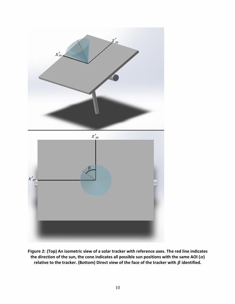
the line between the module’s center and the module’s “top” as illustrated in Figure 2. For

example, consider the tracker pointing at an orientation (𝜃𝑇𝐴, 𝜃𝑇𝐸) of (0°, 0°), i.e., the tracker

face is a plane perpendicular to the earth’s surface with the module’s “top” being up and module

normal pointed north. Consider a coordinate system on the module’s face where 0° points “up”

toward the zenith, 90° points east, 180° points down (toward Earth), and 270° points west. If a

vector from the tracker face to the sun is projected (or “collapsed”) onto the tracker face, 𝛽 is the

measure of the angle counterclockwise from 0° on the tracker face. Because the coordinate

system is referenced to the tracker face, it moves relative to the earth as the tracker rotates.

10

Figure 2: (Top) An isometric view of a solar tracker with reference axes. The red line indicates the direction of the sun, the cone indicates all possible sun positions with the same AOI (𝜶)

relative to the tracker. (Bottom) Direct view of the face of the tracker with 𝜷 identified.

11

2. CALCULATION OF VARIABLES

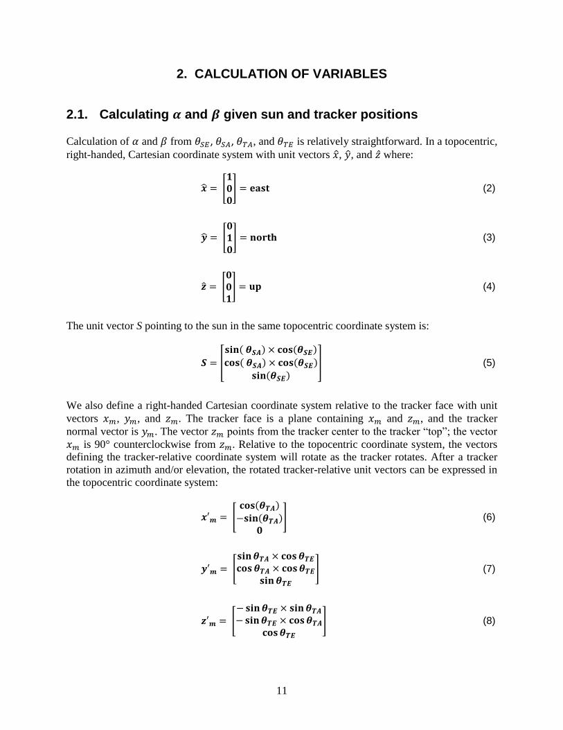
2.1. Calculating 𝜶 and 𝜷 given sun and tracker positions

Calculation of 𝛼 and 𝛽 from 𝜃𝑆𝐸 , 𝜃𝑆𝐴, 𝜃𝑇𝐴, and 𝜃𝑇𝐸 is relatively straightforward. In a topocentric,

right-handed, Cartesian coordinate system with unit vectors �̂�, �̂�, and �̂� where:

�̂� = [𝟏𝟎𝟎

] = 𝐞𝐚𝐬𝐭 (2)

�̂� = [𝟎𝟏𝟎

] = 𝐧𝐨𝐫𝐭𝐡 (3)

�̂� = [𝟎𝟎𝟏

] = 𝐮𝐩 (4)

The unit vector S pointing to the sun in the same topocentric coordinate system is:

𝑺 = [

𝐬𝐢𝐧( 𝜽𝑺𝑨) × 𝐜𝐨𝐬(𝜽𝑺𝑬)

𝐜𝐨𝐬( 𝜽𝑺𝑨) × 𝐜𝐨𝐬(𝜽𝑺𝑬)

𝐬𝐢𝐧(𝜽𝑺𝑬)] (5)

We also define a right-handed Cartesian coordinate system relative to the tracker face with unit

vectors 𝑥𝑚, 𝑦𝑚, and 𝑧𝑚. The tracker face is a plane containing 𝑥𝑚 and 𝑧𝑚, and the tracker

normal vector is 𝑦𝑚. The vector 𝑧𝑚 points from the tracker center to the tracker “top”; the vector

𝑥𝑚 is 90° counterclockwise from 𝑧𝑚. Relative to the topocentric coordinate system, the vectors

defining the tracker-relative coordinate system will rotate as the tracker rotates. After a tracker

rotation in azimuth and/or elevation, the rotated tracker-relative unit vectors can be expressed in

the topocentric coordinate system:

𝒙′𝒎 = [𝐜𝐨𝐬(𝜽𝑻𝑨)

−𝐬𝐢𝐧(𝜽𝑻𝑨)𝟎

] (6)

𝒚′𝒎 = [

𝐬𝐢𝐧 𝜽𝑻𝑨 × 𝐜𝐨𝐬 𝜽𝑻𝑬

𝐜𝐨𝐬 𝜽𝑻𝑨 × 𝐜𝐨𝐬 𝜽𝑻𝑬

𝐬𝐢𝐧 𝜽𝑻𝑬

] (7)

𝒛′𝒎 = [

− 𝐬𝐢𝐧 𝜽𝑻𝑬 × 𝐬𝐢𝐧 𝜽𝑻𝑨

− 𝐬𝐢𝐧 𝜽𝑻𝑬 × 𝐜𝐨𝐬 𝜽𝑻𝑨

𝐜𝐨𝐬 𝜽𝑻𝑬

] (8)

12

As S is a unit vector pointing to the sun, and 𝑦′𝑚 is a unit vector describing the rotated tracker

normal in the same topocentric coordinates, the angle of incidence 𝛼 may be found easily using

equation 9.

𝐜𝐨𝐬(𝛂) = 𝑺 ∙ 𝒚′𝒎 = 𝐬𝐢𝐧 𝜽𝑺𝑬 × 𝐬𝐢𝐧 𝜽𝑻𝑬 + 𝐜𝐨𝐬 𝜽𝑺𝑬 × 𝐜𝐨𝐬 𝜽𝑻𝑬 × 𝐜𝐨𝐬(𝜽𝑺𝑨 − 𝜽𝑻𝑨) (9)

where ∙ is the usual dot product.

By projecting the sun vector S onto the rotated tracker surface, defined by 𝑥′𝑚 and 𝑧′𝑚, we

obtain the angle of incidence direction 𝛽 as shown in equations 10 through 12.

(𝑺 ∙ 𝒙′𝒎) = 𝐜𝐨𝐬 𝜽𝑺𝑬 × 𝐜𝐨𝐬 𝜽𝑻𝑨 × 𝐬𝐢𝐧 𝜽𝑺𝑨 − 𝐜𝐨𝐬 𝜽𝑺𝑬 × 𝐜𝐨𝐬 𝜽𝑺𝑨 × 𝐬𝐢𝐧 𝜽𝑻𝑨 (10)

(𝑺 ∙ 𝒛′𝒎) = 𝐜𝐨𝐬 𝜽𝑻𝑬 × 𝐬𝐢𝐧 𝜽𝑺𝑬 − 𝐬𝐢𝐧 𝜽𝑻𝑬 × 𝐜𝐨𝐬 𝜽𝑺𝑬 × 𝐜𝐨𝐬(𝜽𝑺𝑨 − 𝜽𝑻𝑨) (11)

𝜷 = atan2[(𝑺 ∙ 𝒙′𝒎), (𝑺 ∙ 𝒛′𝒎)] (12)

where atan2(y, x) is the four quadrant arctangent of 𝑦

𝑥; for example, atan2(2, -3) ≈ 146.3°.

2.2. Calculating tracker position given sun position, 𝛂, and 𝛃

The inverse problem, calculating the appropriate tracker rotations 𝜃𝑇𝐴 and 𝜃𝑇𝐸 to achieve desired

𝛼 and 𝛽, given 𝜃𝑆𝐸 and 𝜃𝑆𝐴, is considerably more difficult and in fact may have more than one

solution, or no solution. For example, if the sun is south at 45° elevation (i.e., θSE = 45°, and

𝜃𝑆𝐴 = 180°) and it is desired that 𝛼 = 45° and 𝛽 = 0° (i.e., AOI = 45° and AOI direction is

towards the top of the tracker) then two solutions exist: 𝜃𝑇𝐴 = 180° and 𝜃𝑇𝐸 = 0° (i.e., the

tracker normal is pointed south at the horizon and the tracker top is up), and 𝜃𝑇𝐴 = 0° and

𝜃𝑇𝐸 = 90° (i.e., the tracker normal is pointed straight upwards and the tracker top is pointed

south). We calculate 𝜃𝑇𝐴 and 𝜃𝑇𝐸 using the following algorithm that accommodates cases where

more than one solution, or no solution, exists. Because 𝜃𝑇𝐴 and 𝜃𝑇𝐸 are dependent upon sun

position, the algorithm must be continually performed to accommodate the sun’s movement

through the sky (relative to the topocentric observer).

Generally, 𝜃𝑇𝐴 and 𝜃𝑇𝐸 may be found by simultaneously solving equations 9 and 12. In order to

simplify the resulting expressions we make the following substitutions:

𝑪 = 𝐜𝐨𝐬 𝜽𝑺𝑬 (13)

𝑵 = 𝐬𝐢𝐧 𝜽𝑺𝑬 (14)

𝑫 = 𝐭𝐚𝐧 𝜷 (15)

𝑨 = 𝐜𝐨𝐬 𝜶 (16)

13

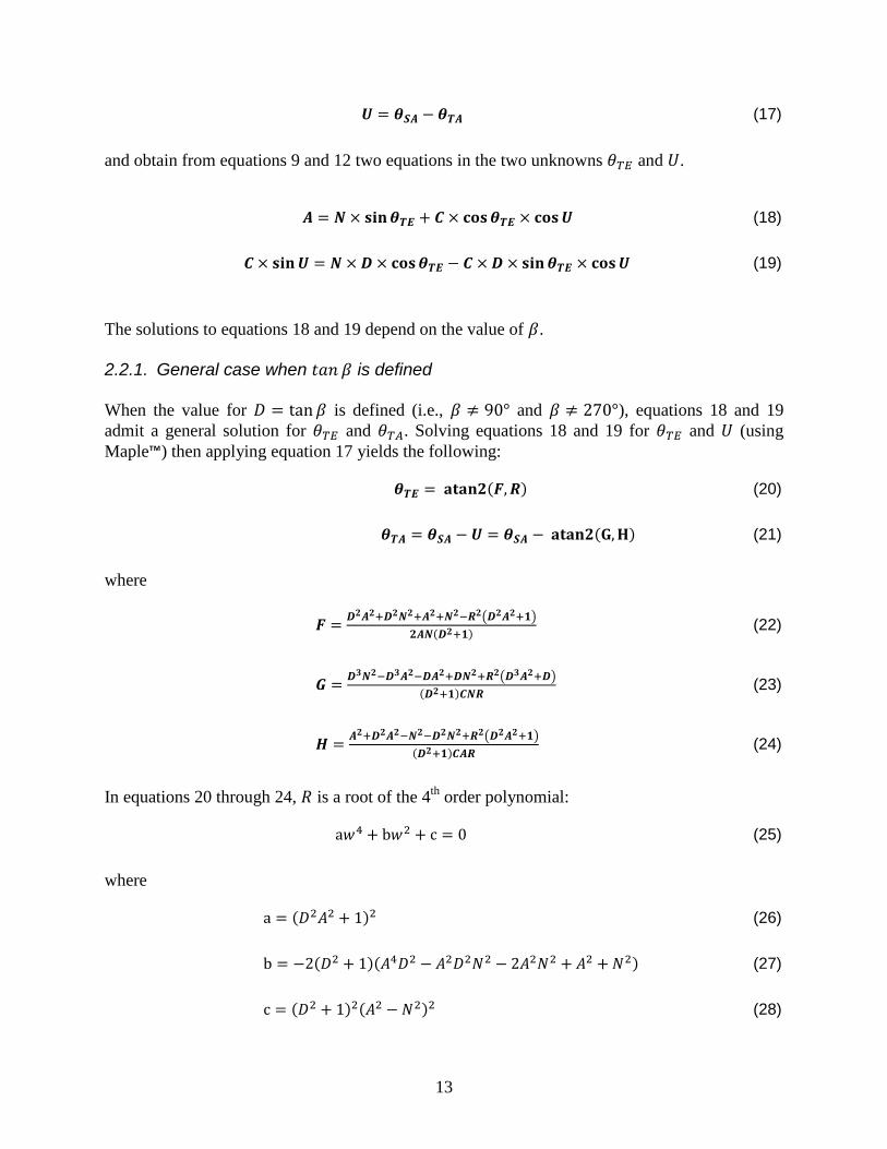
𝑼 = 𝜽𝑺𝑨 − 𝜽𝑻𝑨 (17)

and obtain from equations 9 and 12 two equations in the two unknowns 𝜃𝑇𝐸 and 𝑈.

𝑨 = 𝑵 × 𝐬𝐢𝐧 𝜽𝑻𝑬 + 𝑪 × 𝐜𝐨𝐬 𝜽𝑻𝑬 × 𝐜𝐨𝐬 𝑼 (18)

𝑪 × 𝐬𝐢𝐧 𝑼 = 𝑵 × 𝑫 × 𝐜𝐨𝐬 𝜽𝑻𝑬 − 𝑪 × 𝑫 × 𝐬𝐢𝐧 𝜽𝑻𝑬 × 𝐜𝐨𝐬 𝑼 (19)

The solutions to equations 18 and 19 depend on the value of 𝛽.

2.2.1. General case when 𝑡𝑎𝑛 𝛽 is defined

When the value for 𝐷 = tan 𝛽 is defined (i.e., 𝛽 ≠ 90° and 𝛽 ≠ 270°), equations 18 and 19

admit a general solution for 𝜃𝑇𝐸 and 𝜃𝑇𝐴. Solving equations 18 and 19 for 𝜃𝑇𝐸 and 𝑈 (using

Maple™) then applying equation 17 yields the following:

𝜽𝑻𝑬 = 𝐚𝐭𝐚𝐧𝟐(𝑭, 𝑹) (20)

𝜽𝑻𝑨 = 𝜽𝑺𝑨 − 𝑼 = 𝜽𝑺𝑨 − 𝐚𝐭𝐚𝐧𝟐(𝐆, 𝐇) (21)

where

𝑭 =𝑫𝟐𝑨𝟐+𝑫𝟐𝑵𝟐+𝑨𝟐+𝑵𝟐−𝑹𝟐(𝑫𝟐𝑨𝟐+𝟏)

𝟐𝑨𝑵(𝑫𝟐+𝟏) (22)

𝑮 =𝑫𝟑𝑵𝟐−𝑫𝟑𝑨𝟐−𝑫𝑨𝟐+𝑫𝑵𝟐+𝑹𝟐(𝑫𝟑𝑨𝟐+𝑫)

(𝑫𝟐+𝟏)𝑪𝑵𝑹 (23)

𝑯 =𝑨𝟐+𝑫𝟐𝑨𝟐−𝑵𝟐−𝑫𝟐𝑵𝟐+𝑹𝟐(𝑫𝟐𝑨𝟐+𝟏)

(𝑫𝟐+𝟏)𝑪𝑨𝑹 (24)

In equations 20 through 24, 𝑅 is a root of the 4th

order polynomial:

a𝑤4 + b𝑤2 + c = 0 (25)

where

a = (𝐷2𝐴2 + 1)2 (26)

b = −2(𝐷2 + 1)(𝐴4𝐷2 − 𝐴2𝐷2𝑁2 − 2𝐴2𝑁2 + 𝐴2 + 𝑁2) (27)

c = (𝐷2 + 1)2(𝐴2 − 𝑁2)2 (28)

14

The polynomial in equation 25 admits 0, 2, or 4 real solutions (counting repeated roots). Because

equation 25 is quadratic in form, we can classify the roots, and the solutions 𝜃𝑇𝐸 and 𝜃𝑇𝐴, in

terms of the discriminant, b2 − 4ac.

Case 1: 𝐛𝟐 − 𝟒𝐚𝐜 < 𝟎

When b2 − 4ac < 0, there are no real roots 𝑅 and thus no possible solution for 𝜃𝑇𝐸 and 𝜃𝑇𝐴

given the sun position and the desired values of 𝛼 and 𝛽.

Case 2: 𝐛𝟐 − 𝟒𝐚𝐜 ≥ 𝟎

When b2 − 4ac ≥ 0 there are either two or four real roots 𝑅 counting repeated values:

{+√−𝐛+√𝐛𝟐−𝟒𝐚𝐜

𝟐𝐚, −√−𝐛+√𝐛𝟐−𝟒𝐚𝐜

𝟐𝐚, +√−𝐛−√𝐛𝟐−𝟒𝐚𝐜

𝟐𝐚, −√−𝐛−√𝐛𝟐−𝟒𝐚𝐜

𝟐𝐚} (29)

However, two of the possible solutions for 𝜃𝑇𝐸 and 𝜃𝑇𝐴are extraneous; we denote the values of 𝑅

which correspond to the two actual solutions as

𝑹𝟏 = 𝝀𝟏√−𝐛+√𝐛𝟐−𝟒𝐚𝐜

𝟐𝐚 (30)

𝑹𝟐 = 𝝀𝟐√−𝐛−√𝐛𝟐−𝟒𝐚𝐜

𝟐𝐚 (31)

where 𝜆1 and 𝜆2 are either +1 or -1.

Values for 𝜆1 and 𝜆2 are found by:

𝝀𝟏 = 𝐬𝐠𝐧(𝐜𝐨𝐬 𝜷) (32)

𝛌𝟐 = 𝐬𝐠𝐧(𝐜𝐨𝐬 𝜷) × 𝐬𝐠𝐧[− 𝐜𝐨𝐬(𝜶 + 𝜽𝑺𝑬)] (33)

where sgn(x) denotes the sign or signum function of x. Equations 30 through 33 were developed

empirically by examining all four possible solutions deriving from equation 29, and selecting the

two solutions which lie in the desired AOI direction (upwards on the module, corresponding to

cos 𝛽 ≥ 0, or downwards). The two extraneous solutions lie in the opposite directions.

When 𝛼 + 𝜃𝑆𝐸 ≠ 90° it can be shown that 𝑅1 and 𝑅2 are distinct, and hence there are two

different solutions for (𝜃𝑇𝐸 , 𝜃𝑇𝐴) both of which satisfy equations 18 and 19. Thus, when

𝛼 + 𝜃𝑆𝐸 ≠ 90° and b2 − 4ac ≥ 0 there are two tracker pointing directions which provide the

desired values for 𝛼 and 𝛽; one obtained with 𝑅 = 𝑅1, and a second obtained with 𝑅 = 𝑅2.

15

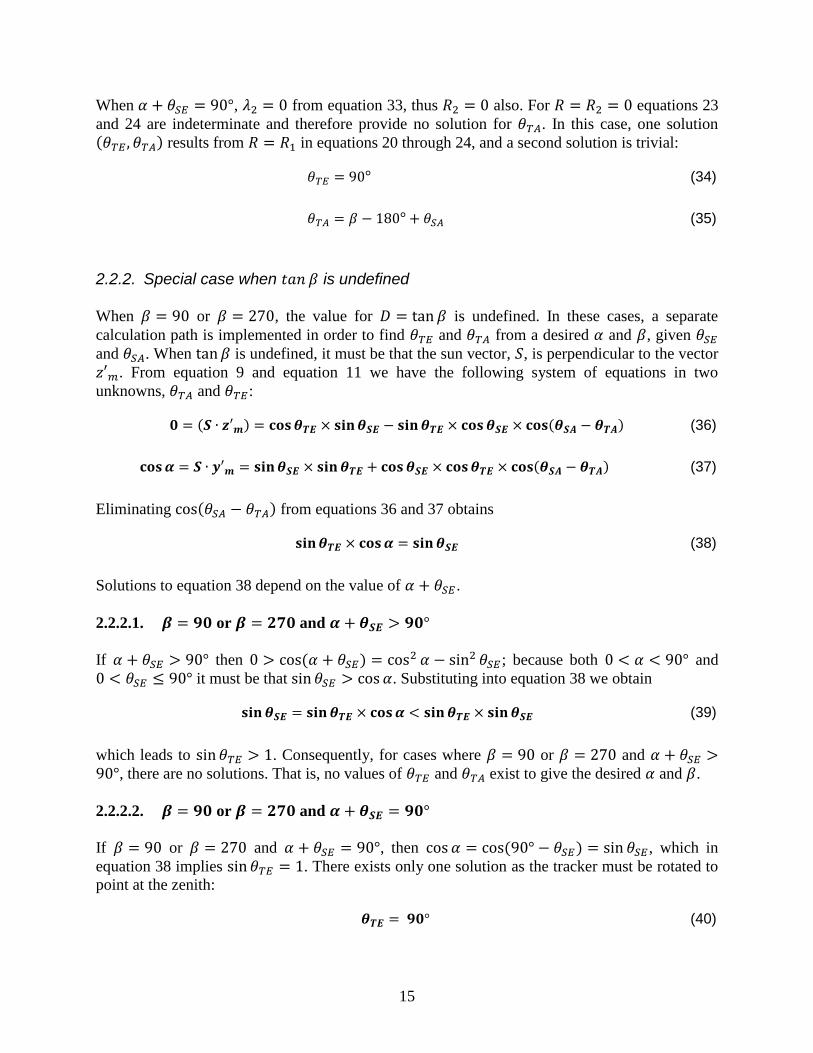
When 𝛼 + 𝜃𝑆𝐸 = 90°, 𝜆2 = 0 from equation 33, thus 𝑅2 = 0 also. For 𝑅 = 𝑅2 = 0 equations 23

and 24 are indeterminate and therefore provide no solution for 𝜃𝑇𝐴. In this case, one solution (𝜃𝑇𝐸 , 𝜃𝑇𝐴) results from 𝑅 = 𝑅1 in equations 20 through 24, and a second solution is trivial:

𝜃𝑇𝐸 = 90° (34)

𝜃𝑇𝐴 = 𝛽 − 180° + 𝜃𝑆𝐴 (35)

2.2.2. Special case when 𝑡𝑎𝑛 𝛽 is undefined

When 𝛽 = 90 or 𝛽 = 270, the value for 𝐷 = tan 𝛽 is undefined. In these cases, a separate

calculation path is implemented in order to find 𝜃𝑇𝐸 and 𝜃𝑇𝐴 from a desired 𝛼 and 𝛽, given 𝜃𝑆𝐸

and 𝜃𝑆𝐴. When tan 𝛽 is undefined, it must be that the sun vector, 𝑆, is perpendicular to the vector

𝑧′𝑚. From equation 9 and equation 11 we have the following system of equations in two

unknowns, 𝜃𝑇𝐴 and 𝜃𝑇𝐸:

𝟎 = (𝑺 ∙ 𝒛′𝒎) = 𝐜𝐨𝐬 𝜽𝑻𝑬 × 𝐬𝐢𝐧 𝜽𝑺𝑬 − 𝐬𝐢𝐧 𝜽𝑻𝑬 × 𝐜𝐨𝐬 𝜽𝑺𝑬 × 𝐜𝐨𝐬(𝜽𝑺𝑨 − 𝜽𝑻𝑨) (36)

𝐜𝐨𝐬 𝜶 = 𝑺 ∙ 𝒚′𝒎 = 𝐬𝐢𝐧 𝜽𝑺𝑬 × 𝐬𝐢𝐧 𝜽𝑻𝑬 + 𝐜𝐨𝐬 𝜽𝑺𝑬 × 𝐜𝐨𝐬 𝜽𝑻𝑬 × 𝐜𝐨𝐬(𝜽𝑺𝑨 − 𝜽𝑻𝑨) (37)

Eliminating cos(𝜃𝑆𝐴 − 𝜃𝑇𝐴) from equations 36 and 37 obtains

𝐬𝐢𝐧 𝜽𝑻𝑬 × 𝐜𝐨𝐬 𝜶 = 𝐬𝐢𝐧 𝜽𝑺𝑬 (38)

Solutions to equation 38 depend on the value of 𝛼 + 𝜃𝑆𝐸 .

2.2.2.1. 𝜷 = 𝟗𝟎 or 𝜷 = 𝟐𝟕𝟎 and 𝜶 + 𝜽𝑺𝑬 > 𝟗𝟎°

If 𝛼 + 𝜃𝑆𝐸 > 90° then 0 > cos(𝛼 + 𝜃𝑆𝐸) = cos2 𝛼 − sin2 𝜃𝑆𝐸 ; because both 0 < 𝛼 < 90° and

0 < 𝜃𝑆𝐸 ≤ 90° it must be that sin 𝜃𝑆𝐸 > cos 𝛼. Substituting into equation 38 we obtain

𝐬𝐢𝐧 𝜽𝑺𝑬 = 𝐬𝐢𝐧 𝜽𝑻𝑬 × 𝐜𝐨𝐬 𝜶 < 𝐬𝐢𝐧 𝜽𝑻𝑬 × 𝐬𝐢𝐧 𝜽𝑺𝑬 (39)

which leads to sin 𝜃𝑇𝐸 > 1. Consequently, for cases where 𝛽 = 90 or 𝛽 = 270 and 𝛼 + 𝜃𝑆𝐸 >90°, there are no solutions. That is, no values of 𝜃𝑇𝐸 and 𝜃𝑇𝐴 exist to give the desired 𝛼 and 𝛽.

2.2.2.2. 𝜷 = 𝟗𝟎 or 𝜷 = 𝟐𝟕𝟎 and 𝜶 + 𝜽𝑺𝑬 = 𝟗𝟎°

If 𝛽 = 90 or 𝛽 = 270 and 𝛼 + 𝜃𝑆𝐸 = 90°, then cos 𝛼 = cos(90° − 𝜃𝑆𝐸) = sin 𝜃𝑆𝐸 , which in

equation 38 implies sin 𝜃𝑇𝐸 = 1. There exists only one solution as the tracker must be rotated to

point at the zenith:

𝜽𝑻𝑬 = 𝟗𝟎° (40)

16

𝜽𝑻𝑨 = 𝜷 − 𝟏𝟖𝟎° + 𝜽𝑺𝑨 (41)

2.2.2.3. 𝜷 = 𝟗𝟎 or 𝜷 = 𝟐𝟕𝟎 and 𝜶 + 𝜽𝑺𝑬 < 𝟗𝟎°

If 𝛽 = 90 or 𝛽 = 270 and 𝛼 + 𝜃𝑆𝐸 < 90°, there exist two solutions. The first solution allows the

tracker to remain “upright”, that is, cos 𝜃𝑇𝐸 ≥ 0, while the second forces the tracker to be

“upside down”. Both solutions for 𝜃𝑇𝐸 follow from solving equation 38. Because 𝛼 < 90° − 𝜃𝑆𝐸

and both 𝜃𝑆𝐸 < 90° and 𝛼 < 90°, it follows that sin 𝜃𝑆𝐸 < sin(90° − 𝛼) = cos 𝛼, thus equation

38 admits two solutions: one in Quadrant I or IV (equation 42)

𝜽𝑻𝑬 = 𝐬𝐢𝐧−𝟏 (𝐬𝐢𝐧 𝜽𝑻𝑬

𝐜𝐨𝐬 𝜶) = 𝐬𝐢𝐧−𝟏 (

𝑵

𝑨) (42)

and a second solution in Quadrant II or III (equation 43):

𝜽𝑻𝑬 = 𝟏𝟖𝟎° − 𝐬𝐢𝐧−𝟏 (𝑵

𝑨) (43)

Note that equations 42 and 43 yield 𝜃𝑇𝐸 values between -90° and 270°. Because we define 𝜃𝑇𝐸 to

values within the range (-180°, 180°], values in the range [180°, 270°] have 360° subtracted from

them to be within the defined limits of 𝜃𝑇𝐸 .

For each value of 𝜃𝑇𝐸 found by equations 42 or 43, the corresponding value for 𝜃𝑇𝐴 is then found

from equation 44.

𝜽𝑻𝑨 = 𝜽𝑺𝑨 − 𝐜𝐨𝐬−𝟏 (𝑨×𝐜𝐨𝐬 𝜽𝑻𝑬

𝑪) ∗ 𝐬𝐢𝐧 𝜷 (44)

Equation 44 is obtained by eliminating terms involving 𝜃𝑇𝐸 from the system comprising

equations 36 and 37.

2.2.3. Special case when 𝑡𝑎𝑛 𝛽 = 0 and 𝜃𝑆𝐸 = 90

When the sun is directly overhead, that is 𝜃𝑆𝐸 = 90, it is clear that only values of 𝛽 which may

be accomplished by an azimuth/elevation tracker are 𝛽 = 0 or 𝛽 = 180. In the case of 𝜃𝑆𝐸 = 90

and 𝛽 = 0 or 𝛽 = 180, the discriminant for equation 25 will be equal to 0. The equations

provided in section 2.2.1 will determine a correct value for 𝜃𝑇𝐸; however, the equations will also

provide a value for 𝜃𝑇𝐴. Under these conditions the value provided for 𝜃𝑇𝐴 is irrelevant, as

rotations in the tracker azimuth do not result in changes of 𝛼 or 𝛽.

17

3. PITFALLS WHEN COMPUTING VALUES NUMERICALLY

For applications of testing solar energy products, a typical implementation of these equations

will require some form of computer. We have found several possible pitfalls to avoid when

numerically evaluating for the solutions of the equations above. Most of these pitfalls arise due

to precision errors when computers manipulate numbers that are then used in checks for equality

or in inequalities.

3.1. Evaluating inverse cosine and inverse sine

Evaluations of inverse trigonometric functions can sometimes be problematic, especially when

the arguments of the inverse function contain approximations of trigonometric functions, such as

in equations 9, 42, and 43. It is possible, in some situations, to have arguments to the inverse

cosine and inverse sine functions which are slightly above 1 or below -1, in which case the

inverse trigonometric function could be improperly evaluated.

In these cases, it may be prudent to limit arguments to inverse sine and inverse cosine functions

to the interval [-1, 1] prior to evaluation.

3.2. Comparison for equality

Some of the equations presented above involve evaluating for equalities or inequalities, for

example, in section 2.2.2 there is a comparison to determine if 𝛼 + 𝜃𝑆𝐸 = 90°. In situations such

as these, precision errors may again cause values which should be equivalent to evaluate as

unequal. One possible solution to these precision errors is to evaluate if the values are nearly

equivalent. For example, one may evaluate the equality comparison of 𝛼 + 𝜃𝑆𝐸 = 90 as |𝛼 +𝜃𝑆𝐸 − 90| < 𝜀, where 𝜀 is a small positive number which is larger than the numeric precision of

the calculation platform.

3.3. Evaluating when 𝛉𝐒𝐄 is 0

As stated previously, the sun elevation, 𝜃𝑆𝐸 , is defined over the interval [-90°, 90°], yet the

equations listed above should only be used when 𝜃𝑆𝐸 > 0. If 𝜃𝑆𝐸 is 0, then sin(𝜃𝑆𝐸) = 𝑁 = 0 and

equations 22 and 23 are undefined. It is therefore recommended to set θSE to a small positive

value (perhaps 0.0001) for extremely low sun angles; while doing so introduces some small error

in the tracker pointing solution, the deviation is probably insignificant compared to error in the

apparent sun position caused by miscalculation of atmospheric refraction or to effects introduced

by near shading or far shading.

18

19

4. CONCLUSIONS

Sandia National Laboratories has developed a system whereby the angle between direct beam

sunlight and a terrestrial plane (e.g. a photovoltaic module, solar tracker face) may be described

both by the angle of incidence and the direction which the beam falls on the plane. These values,

denoted 𝛼 and 𝛽 respectively, are simple to calculate using equations 9 through 12 when given

the sun position and the pointing direction of a 2-axis solar tracker employing azimuth and

elevation rotation axes.

It is more difficult, however, to determine the correct pointing angles, 𝜃𝑇𝐴 and 𝜃𝑇𝐸 , of an

azimuth/elevation two-axis solar tracker that obtain a desired 𝛼 and 𝛽 for a given sun position.

We describe an algorithm for determination of these tracker pointing angles when the sun is

above the horizon. It is possible that there may be 0, 1, or 2 tracker orientations which provide

the desired 𝛼 and 𝛽, and the choice of which orientation is best for any application is left to the

implementer.

20

21

5. REFERENCES

1. D.L. King, W.E. Boyson, J.A. Kratochvil. Photovoltaic Array Performance Model,

SAND2004-3535, Sandia National Laboratories, Albuquerque, NM, Unlimited Release,

December 2004.

22

23

DISTRIBUTION

1 MS0951 Daniel Riley 6112

1 MS1033 Charles Hanley 6112

1 MS1033 Clifford Hansen 6112

1 MS1033 Abraham Ellis 6112

1 MS0899 Technical Library 9536 (electronic copy)

24