SUMMER PROJECT May-June, 2011

DEVELOPMENT OF A SELF

BALANCING BICYCLE ROBOT

BY

SUBHOJIT GHOSH AND RAJAT ARORA

Y9599 Y9464

Department of Mechanical Engineering

Indian Institute of Technology

Kanpur

UNDER THE GUIDANCE OF:

Prof. Bishakh Bhattacharya

Department of Mechanical Engineering

IIT Kanpur

ABSTRACT

Two wheeled balancing robots are based on inverted pendulum

configurations which rely upon dynamic balancing systems for

balancing and manoeuvring. As the name suggest the robot would

be a bicycle that can move forward or backward, controlled

through a wireless remote, and at the same time autonomously

balancing itself and avoid falling.

Why not just make a 4-wheeled or 3-wheeled robot?

The following are some reasons:

A bicycle uses less track space as compared to any other

vehicle.

It is more flexible and easy to steer as compared to any other

vehicle.

It can cut through obstacles easier than a four wheeled bot.

This technology can be extended to make a self balancing

unicycle which is much better in terms of space and steer

ability.

Due to its low weight and greater steer ability, it can be made

faster than a humanoid robot.

This robot might be useful for transportation in research areas

or mines where man or four wheeled robots cannot reach.

In particular, the focus is on the electro-mechanical mechanisms &

control algorithms required to enable the robot to perceive and act

in real time for a dynamically changing world. The construction of

sensors, filters and actuator system is a learning experience.

INTRODUCTION

Two wheeled balancing robot is a classic engineering problem

based on inverted pendulum and is much like trying to balance a

broom on the tip of your finger. This challenging robotics,

electronics, and controls problem is the basis of our study for this

project.

BALANCING PROCESS: PLAN OF ACTION

The word ‘balance’, here, means that the inverted pendulum is in

equilibrium state, i.e. its position is standing upright at 90 degrees.

However, the system itself is not balanced, which means it keeps

falling off, away from the vertical axis. The same concept is used

here in the form of a Reaction Wheel Pendulum. A flywheel is

attached to an electric motor whose speed can be controlled. Here

we exploit the fact that when the motors apply torque to rotate the

flywheel, they experience a reactionary torque themselves.

Therefore, an accelerometer-gyroscopic inertial measurement

unit is needed to provide the angular position or tilt of the robot

base with respect to the vertical and input it to the microcontroller,

which is programmed with a balancing algorithm. The

microcontroller will provide a type of feedback signal through

Pulse Width Modulation (PWM) control to the MOSFET

reinforced L293 motor driver’s H-Bridge circuit to turn the motor

clockwise or anticlockwise with appropriate speed and

acceleration, based on the Proportional-Integral-Derivative

(PID) control, thus balancing the robot.

The code is written in C software (Code Vision AVR) and

compiled for the Atmel ATMega16 microcontroller through AVR

Studio, the MCU being interfaced with the sensors and motors.

The main goal of the microcontroller is to fuse the wheel encoder,

gyroscope and accelerometer sensors through a method called

Kalman Filtering, to estimate the attitude of the platform and then

to use this information to drive the reaction wheel in the direction

to maintain an upright and balanced position.

The basic idea for a two-wheeled dynamically balancing robot is

pretty simple: move the actuator in a direction to counter the

direction of fall. In practice this requires two feedback sensors: a

tilt or angle sensor to measure the tilt of the robot with respect to

gravity, an accelerometer to calibrate the gyro thus minimizing the

drift. Two terms are used to balance the robot. These are 1) the tilt

angle and 2) its first derivative, the angular velocity. These two

measurements are summed together through Kalman Filtering and

fed back to the actuator which produces the counter torque

required to balance the robot through PID.

Thus the robot can be classified into the following parts:

Mechanical Model

Inertial sensors

Logical processing unit

Actuators (Wireless Drive-Motor and Flywheel Control)

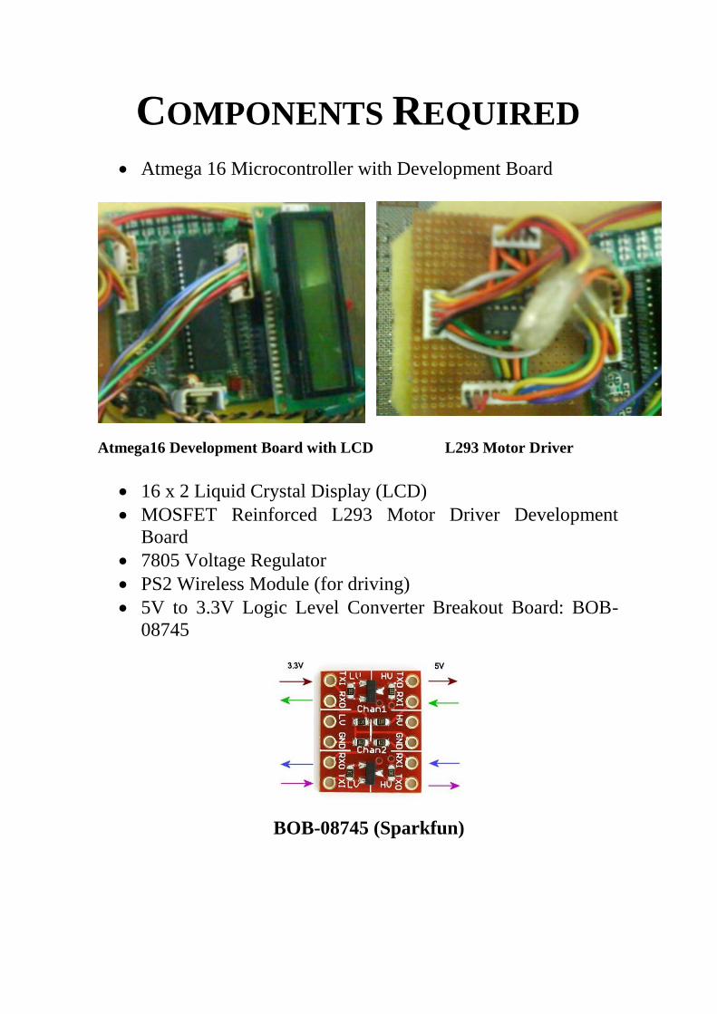
COMPONENTS REQUIRED

Atmega 16 Microcontroller with Development Board

Atmega16 Development Board with LCD L293 Motor Driver

16 x 2 Liquid Crystal Display (LCD)

MOSFET Reinforced L293 Motor Driver Development

Board

7805 Voltage Regulator

PS2 Wireless Module (for driving)

5V to 3.3V Logic Level Converter Breakout Board: BOB-

08745

BOB-08745 (Sparkfun)

USB based STK500 Programmer for AVR MCUs (with

Atmega8 and 74126 ICs)

STK500 Programmer

Connectors and Wires, other tools, Lithium ion batteries.

Aluminium Angles

Mica Sheet

Mechanical Accessories: Couplers, Bushings, Shafts, Pulleys,

Track-belts, Sprockets, Chains

2 Thin Tyres of Diameter 9-12 cm.

Flywheel (Lathed)

High Torque 300 RPM DC Motor operating at 24V(Mech-

Tex)

Low Torque DC Motor for Driving (12V)

Inertial Measurement Unit (IMU) from Sparkfun: 5 Degree

of Freedom Analog Combo Board with Triple Axis

Accelerometer ADXL335 and Dual Axis Gyroscope

IDG500.

5 DOF IMU Combo Board

MECHANICAL MODEL

The whole bicycle is constructed with the help of aluminium

angles and mica sheet. The mica sheet portions allow for drive-

motor mounting and keeping electrical circuitry. The cycle is

low-lying so as to make its centre of mass low.

Flywheel is made of mild steel, and it is sufficiently heavy

enough to provide enough reactionary torque in the high torque

motor attached to the vertical aluminium angles.

Reaction Wheel

The front wheel is free and attached with the help of a threaded

axle and bushings. As the bicycle had to be kept thin, with its

centre of mass low and exactly in the plane of the bicycle, so the

driving motor had to be attached parallel to the axis of the

driven wheel.

The rear wheel is driven by the drive-motor with the help of a

link system. Both chain-sprocket system as well as track belt-

pulley system can be used. These accessories are attached to the

wheel’s axle with the help of couplers.

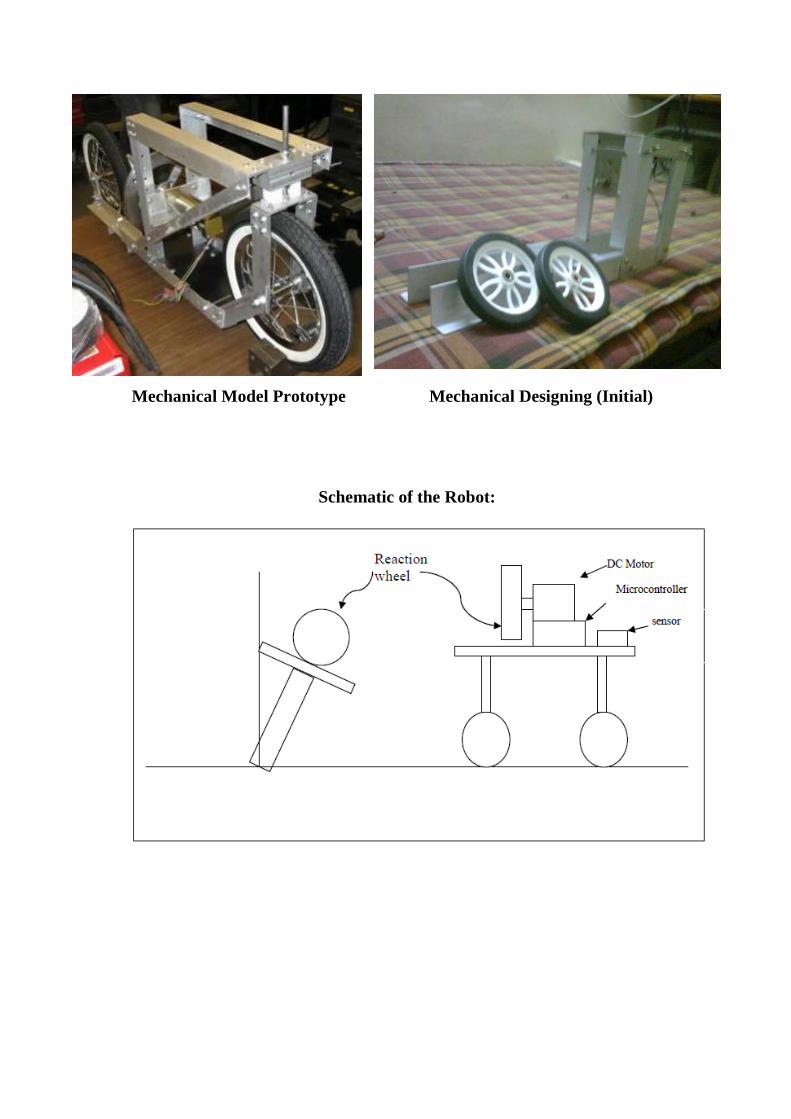
Mechanical Model Prototype Mechanical Designing (Initial)

Schematic of the Robot:

INERTIAL MEASUREMENT

UNIT: TILT SENSOR MODULE

Tilt sensing is the crux of this project and the most difficult part as

well. The inertial sensors used here (in IMU Combo board) are:

Triple Axis Accelerometer ADXL335

Dual Axis Gyroscope IDG500

An accelerometer measures the acceleration in specific directions.

We can measure the direction of gravity w.r.t the accelerometer

and get the tilt angle w.r.t the vertical. It is free from drifts and

other errors. The angle of tilt can be measured from the

acceleration along x-direction as follows:

Ax = g sin θ (θ is the angle w.r.t vertical)

Az = g cos θ (Ax, Az are accelerations in x

and z directions)

For small angles, Ax = g θ

So, θ = K * Ax (K is a constant)

We use this formula since inverse

trigonometric calculations in the MCU may

be time consuming.

The accelerometer outputs an analog voltage Va, and acceleration

can be measured by the formula:

Acceleration = (Va – Vat zero tilt)/Sensitivity (in V/‘g’)

This approach is correct, but only for slow angular velocities, at

high angular velocities the accelerometer tilt angle begins to lag

giving wrong tilt data.

This problem is solved by using a Gyroscope. It would measure

angular velocity and angle can be found by integrating.

The rate gyro measures angular velocity and outputs a voltage Vg:

Vg= ω + f(T) + eg

Where f(T) represents the effect of temperature and eg represents

error, which is not known. So the correct formula is:

Angular Velocity ω = (Vg – Vat zero tilt)/Sensitivity [in V/(deg/s)]

But this approach fails at slow angular velocities due to gyroscopic

drift (small errors in slow velocities integrate and accumulate into

a big error).

In reality, we do not have static conditions, but dynamic

conditions. So in case of dynamic accelerations, the accelerometer

and gyroscope outputs are combined together using the Kalman

Filtering Method. The Kalman filter is a mathematical method

named after Rudolf E. Kalman. Its purpose is to use measurements

that are observed over time that contain noise (random variations)

and other inaccuracies, and produce values that tend to be closer to

the true values of the measurements and their associated calculated

values.

Ax = g sin θ - δvx/δt

θ = K * (Ax + rώ) (For small θ, ώt is angular acceleration)

For calculating the integrals and derivatives, PID algorithm is:

Calculation of θt by integration; (suffix t stands for time t)

θt = θt-1 + ω*δt

Calculation of ώt by differentiation;

ώt = ( ωt – ωt-1)/ δt

The code for Kalman Filtering is as follows:

static const double dt = 0.032;

static double P[2][2] = {{ 1, 0 },{ 0, 1 }};

double angle;

double q_bias;

double rate;

static const double R_angle = 0.300;

static const double Q_angle = 0.001;

static const double Q_gyro = 0.003;

void state_update(const double q)

{

double Pdot[2][2];

Pdot[0] [0] = Q_angle - P[0][1] - P[1][0]; /* 0,0 */

Pdot[0] [1] = - P[1][1]; /* 0,1 */

Pdot[1] [0] = - P[1][1]; /* 1,0 */

Pdot[0] [0] = Q_gyro; /* 1,1 */

/* Stores our unbiased gyro estimate */

rate = q;

angle += q * dt;

P[0][0] += Pdot[0] [0]* dt;

P[0][1] += Pdot[0] [1]* dt;

P[1][0] += Pdot[1] [0]* dt;

P[1][1] += Pdot[1] [1]* dt;

}

void kalman_update(double angle_m)

{

double angle_err;

double C_0 = 1;

double PCt_0, PCt_1;

double E, K_0, K_1, t_0, t_1;

angle_err = angle_m - angle;

PCt_0 = C_0 * P[0][0]; /* + C_1 * P[0][1] = 0 */

PCt_1 = C_0 * P[1][0]; /* + C_1 * P[1][1] = 0 */

E = R_angle + C_0 * PCt_0;

K_0 = PCt_0 / E;

K_1 = PCt_1 / E;

t_0 = PCt_0; /* C_0 * P[0][0] + C_1 * P[1][0] */

t_1 = C_0 * P[0][1]; /* + C_1 * P[1][1] = 0 */

P[0][0] -= K_0 * t_0;

P[0][1] -= K_0 * t_1;

P[1][0] -= K_1 * t_0;

P[1][1] -= K_1 * t_1;

Angle += K_0 * angle_err;

q_bias += K_1 * angle_err;

}

void main(void)

{

int x, y, z, dv, ocr, w, anglef=0;

float g,angle2=0,diff=0,integral=0,k;

long zx;

char a[10];// Declare your local variables here

while (1)

{

x=read_adc(3)-330;

y=read_adc(2)-330;

z=read_adc(1)-330;

w=(285-read_adc(0));

zx=z*sqrt(x*x/z/z+1.0);

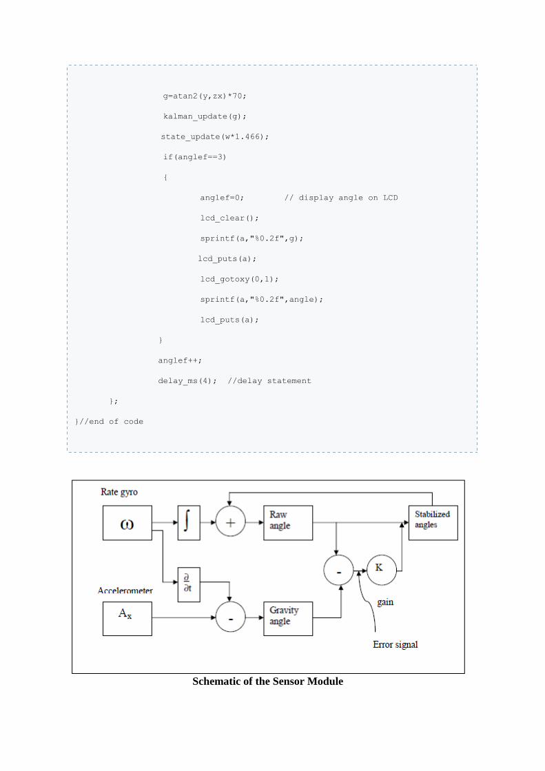
g=atan2(y,zx)*70;

kalman_update(g);

state_update(w*1.466);

if(anglef==3)

{

anglef=0; // display angle on LCD

lcd_clear();

sprintf(a,"%0.2f",g);

lcd_puts(a);

lcd_gotoxy(0,1);

sprintf(a,"%0.2f",angle);

lcd_puts(a);

}

anglef++;

delay_ms(4); //delay statement

};

}//end of code

Schematic of the Sensor Module

LOGICAL PROCESSING UNIT

The processing unit used is Atmel ATMega16 microcontroller unit

which is a versatile EEPROM. It has four I/O (Input/Output) ports,

onboard ADC (Analog to Digital Converter) and PWM (Pulse

Width Modulation) outputs for motor control. It can be

programmed easily with minimum hardware requirements which

make it extremely popular in robotics applications. Here it

performs the following functions:

ADC conversion of outputs of Rate Gyro and Accelerometer

Processing the input signals

Periodic recalibration of gyro

Display of angle & other data.

Control of actuator unit

Schematic of the processing unit is as shown:

Circuit Diagram:

ALGORITHM:

The algorithm for the controller is as follows:

Step1: Initialize the values of rate gyro bias and accelerometer bias

for zero value of θ & ω.

Step2: Measure the value of voltage of gyro and accelerometer

outputs and store those values as ω and Ax.

Step3: Integrate the rate gyro reading by: θt = θt-1 + ω*δt

Differentiate the rate gyro reading by: ώt = (ωt – ωt-1)/ δt

δt in each case is assumed to be constant and is equal to the

cycle time.

Step4: Calculate the raw angle and gravity angle and compute the

error value.

Step5: Update the raw angle by:

θstabilized = θraw angle + constant* (θgravity angle – θraw angle)

Constant is taken as 0.2

Step6: We calculate the torque required to restore balance:

τ = constant * sin θ (or τ = constant * θ for small angles)

Step7: We obtain the direction of rotation of the reaction wheel:

If θ < 0, counter-clockwise

If θ > 0, clockwise

Step8: Send the output to the DC motor attached to the reaction

wheel.

Step9: Repeat steps (2-8)

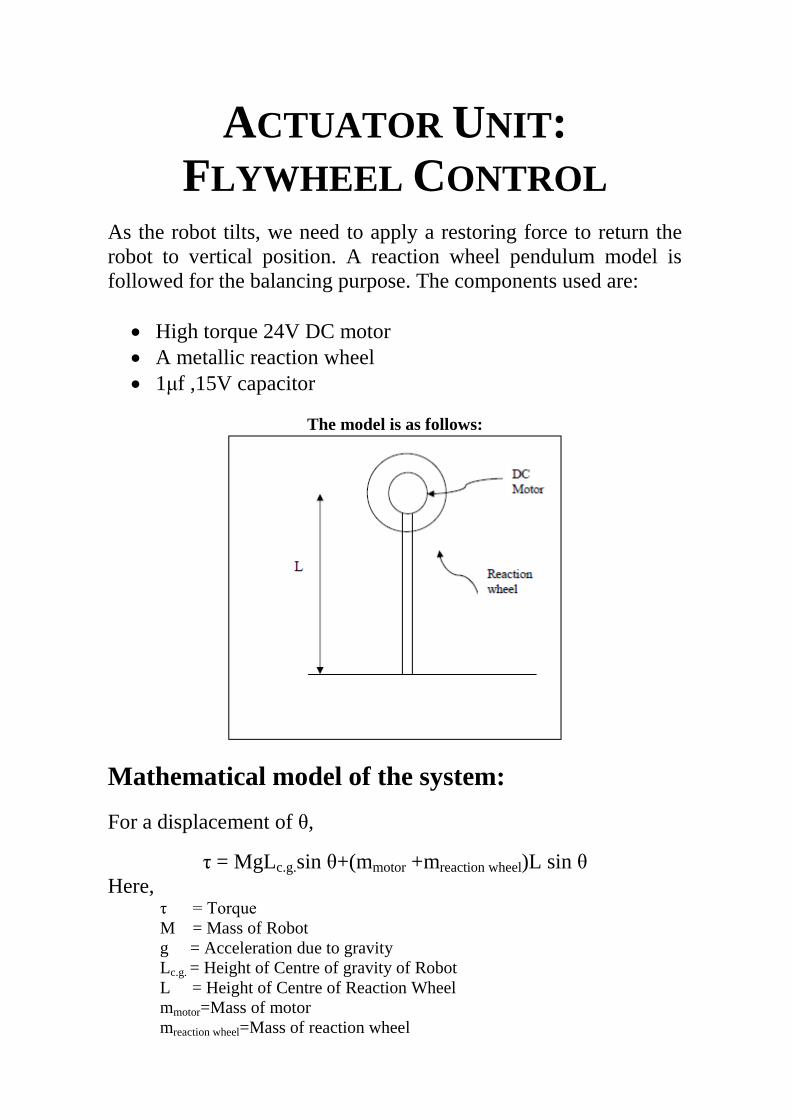
ACTUATOR UNIT:

FLYWHEEL CONTROL

As the robot tilts, we need to apply a restoring force to return the

robot to vertical position. A reaction wheel pendulum model is

followed for the balancing purpose. The components used are:

High torque 24V DC motor

A metallic reaction wheel

1μf ,15V capacitor

The model is as follows:

Mathematical model of the system:

For a displacement of θ,

τ = MgLc.g.sin θ+(mmotor +mreaction wheel)L sin θ

Here, τ = Torque

M = Mass of Robot

g = Acceleration due to gravity

Lc.g. = Height of Centre of gravity of Robot

L = Height of Centre of Reaction Wheel

mmotor=Mass of motor

mreaction wheel=Mass of reaction wheel

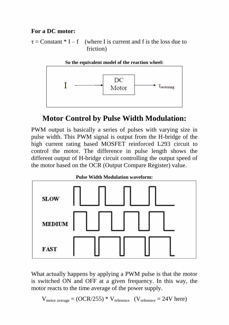
For a DC motor:

τ = Constant * I – f (where I is current and f is the loss due to

friction)

So the equivalent model of the reaction wheel:

Motor Control by Pulse Width Modulation:

PWM output is basically a series of pulses with varying size in

pulse width. This PWM signal is output from the H-bridge of the

high current rating based MOSFET reinforced L293 circuit to

control the motor. The difference in pulse length shows the

different output of H-bridge circuit controlling the output speed of

the motor based on the OCR (Output Compare Register) value.

Pulse Width Modulation waveform:

What actually happens by applying a PWM pulse is that the motor

is switched ON and OFF at a given frequency. In this way, the

motor reacts to the time average of the power supply.

Vmotor average = (OCR/255) * Vreference (Vreference = 24V here)

The capacitor connected across the motor charges and discharges

during the on and off time respectively, thus behaving like an

integrator. The torque generated by the motor is a function of the

average value of current supplied to it.

It seems to be obvious that once we have angle we can rotate the

flywheel with acceleration proportional to it, but that won't do the

job. If that is done what actually will happen is that when there is a

tilt the bike will cross the mean position and reach the other side

till the same tilt angle. To fix this we need some kind of algorithm

that can damp this periodic motion and make it stable at the mean

position after some time. This is where PID (Proportional,

Integral, Derivative) Controller comes to use.

PID Control of Flywheel:

The proportional term makes a change to the output that is

proportional to the current error value. The proportional response

can be adjusted by multiplying the error by a constant Kp, called

the proportional gain. The contribution from the integral term is

proportional to both the magnitude of the error and the duration of

the error. The integral in a PID controller is the sum of the

instantaneous error over time and gives the accumulated offset that

should have been corrected previously. The accumulated error is

then multiplied by the integral gain (Ki) and added to the controller

output. The derivative of the process error is calculated by

determining the slope of the error over time and multiplying this

rate of change by the derivative gain Kd.

The proportional, integral, and derivative terms are summed to

calculate the output of the PID controller. Defining u(t) as the

controller output, the final form of the PID algorithm is:

where: Pout: Proportional term of output

Kp: Proportional gain, a tuning parameter

Ki: Integral gain, a tuning parameter

Kd: Derivative gain, a tuning parameter

e: Error

t: Time or instantaneous time (the present)

We tune the PID controller by varying the constants Kp, Kd and Ki

and optimising them by any well known method (like the Ziegler

Nichol’s Method).

Process Variable (PV) vs time:

So, we use the PID method to control the flywheel for balancing.

The PID Code is as follows:

(The following code is inside the continuous while loop)

dv = kp * angle + ki * integral + kd * diff;

integral += angle;

diff = angle – previous_angle;

previous_angle = angle;

OC1A += dv; //OCR Value changed

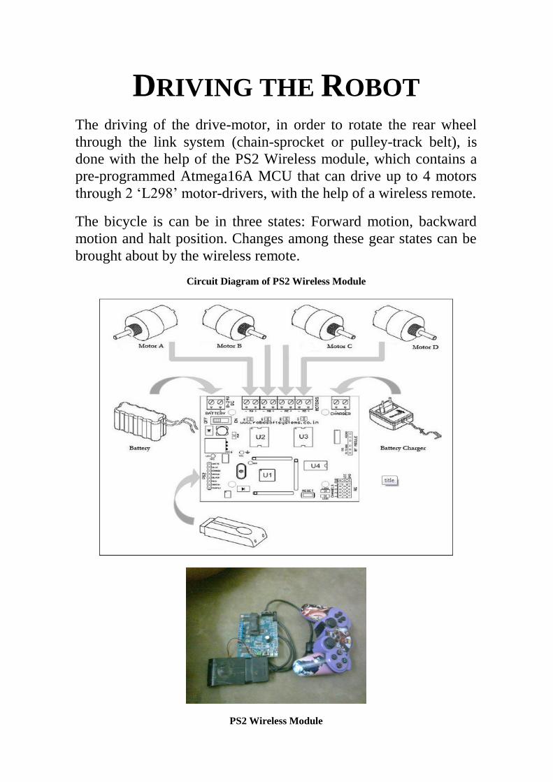
DRIVING THE ROBOT

The driving of the drive-motor, in order to rotate the rear wheel

through the link system (chain-sprocket or pulley-track belt), is

done with the help of the PS2 Wireless module, which contains a

pre-programmed Atmega16A MCU that can drive up to 4 motors

through 2 ‘L298’ motor-drivers, with the help of a wireless remote.

The bicycle is can be in three states: Forward motion, backward

motion and halt position. Changes among these gear states can be

brought about by the wireless remote.

Circuit Diagram of PS2 Wireless Module

PS2 Wireless Module

PRESENT PHOTOS AND VIDEO LINK

COMPLETED ROBOT:

CIRCUITRY:

TEST RUN VIDEO LINK: http://www.youtube.com/watch?v=dNSuuoPgBpU

FUTURE IMPROVEMENTS

In future, the bicycle could be made to move not only forward and

backward, but also steer sideways.

The PS2 Wireless Module has slots for four motors, and can be

made to control a servo motor which could be used to introduce the

steering functionality on to the front wheel.

The balancing can be made much more precise by introducing a

rotating disc whose gyroscopic precession could be used for more

accurate balancing.

In addition, fuzzy logic controller can also be implemented to

provide flexibility and accuracy in control.

ACKNOWLEDGEMENT

We would like to express our deep sense of gratitude and respect to

our supervisor Prof. Bishakh Bhattacharya, for his guidance,

suggestions and support. We consider ourselves extremely lucky to

be able to work under his guidance. We would also like to thank

our friends who have helped us a lot.

SUBHOJIT GHOSH AND RAJAT ARORA

Y9599 Y9464

Department of Mechanical Engineering

Indian Institute of Technology

Kanpur

See Code Next Page...

Code:

/*****************************************************

This program was produced by the

CodeWizardAVR V1.24.6 Standard

Automatic Program Generator

© Copyright 1998-2005 Pavel Haiduc, HP InfoTech s.r.l.

http://www.hpinfotech.com

e-mail:office@hpinfotech.com

Project :

Version :

Date : 27-10-2011

Author : Subhojit

Company : IITK

Comments:

Chip type : ATmega16

Program type : Application

Clock frequency : 8.000000 MHz

Memory model : Small

External SRAM size : 0

Data Stack size : 256

*****************************************************/

#include <mega16.h>

#include <delay.h>

#include <stdio.h>

#include <stdlib.h>

#include <math.h>

// Alphanumeric LCD Module functions

#asm

.equ __lcd_port=0x15 ;PORTC

#endasm

#include <lcd.h>

#define ADC_VREF_TYPE 0x00

// Read the AD conversion result

unsigned int read_adc(unsigned char adc_input)

{

ADMUX=adc_input|ADC_VREF_TYPE;

// Start the AD conversion

ADCSRA|=0x40;

// Wait for the AD conversion to complete

while ((ADCSRA & 0x10)==0);

ADCSRA|=0x10;

return ADCW;

}

// Declare your global variables here

int accx,accy,accz,ratey,ratex,omegax,oc0;

int accx0,accy0,accz0,ratey0,ratex0;

char ch[10];

float theta,theta2,angle,prev_angle,diff,integral,dv;

float kp,kd,ki;

void main(void)

{

// Declare your local variables here

kp=1.5;

kd=6.0;

ki=0.000000;

// Input/Output Ports initialization

// Port A initialization

// Func7=In Func6=In Func5=In Func4=In Func3=In Func2=In Func1=In Func0=In

// State7=T State6=T State5=T State4=T State3=T State2=T State1=T State0=T

PORTA=0x00;

DDRA=0x00;

// Port B initialization

// Func7=In Func6=In Func5=In Func4=In Func3=Out Func2=Out Func1=Out

Func0=Out

// State7=T State6=T State5=T State4=T State3=0 State2=0 State1=0 State0=0

PORTB=0x00;

DDRB=0x0F;

// Port C initialization

// Func7=In Func6=In Func5=In Func4=In Func3=In Func2=In Func1=In Func0=In

// State7=T State6=T State5=T State4=T State3=T State2=T State1=T State0=T

PORTC=0x00;

DDRC=0x00;

// Port D initialization

// Func7=In Func6=Out Func5=In Func4=In Func3=In Func2=In Func1=In Func0=In

// State7=T State6=0 State5=T State4=T State3=T State2=T State1=T State0=T

PORTD=0x00;

DDRD=0x40;

// Timer/Counter 0 initialization

// Clock source: System Clock

// Clock value: 8000.000 kHz

// Mode: Fast PWM top=FFh

// OC0 output: Non-Inverted PWM

TCCR0=0x69;

TCNT0=0x00;

OCR0=0x00;

// Timer/Counter 1 initialization

// Clock source: System Clock

// Clock value: Timer 1 Stopped

// Mode: Normal top=FFFFh

// OC1A output: Discon.

// OC1B output: Discon.

// Noise Canceler: Off

// Input Capture on Falling Edge

// Timer 1 Overflow Interrupt: Off

// Input Capture Interrupt: Off

// Compare A Match Interrupt: Off

// Compare B Match Interrupt: Off

TCCR1A=0x00;

TCCR1B=0x00;

TCNT1H=0x00;

TCNT1L=0x00;

ICR1H=0x00;

ICR1L=0x00;

OCR1AH=0x00;

OCR1AL=0x00;

OCR1BH=0x00;

OCR1BL=0x00;

// Timer/Counter 2 initialization

// Clock source: System Clock

// Clock value: Timer 2 Stopped

// Mode: Normal top=FFh

// OC2 output: Disconnected

ASSR=0x00;

TCCR2=0x00;

TCNT2=0x00;

OCR2=0x00;

// External Interrupt(s) initialization

// INT0: Off

// INT1: Off

// INT2: Off

MCUCR=0x00;

MCUCSR=0x00;

// Timer(s)/Counter(s) Interrupt(s) initialization

TIMSK=0x00;

// Analog Comparator initialization

// Analog Comparator: Off

// Analog Comparator Input Capture by Timer/Counter 1: Off

ACSR=0x80;

SFIOR=0x00;

// ADC initialization

// ADC Clock frequency: 125.000 kHz

// ADC Voltage Reference: AREF pin

// ADC Auto Trigger Source: None

ADMUX=ADC_VREF_TYPE;

ADCSRA=0x86;

// LCD module initialization

lcd_init(16);

delay_ms(1000);

accx0=read_adc(0);

accy0=read_adc(1);

accz0=read_adc(2);

ratex0=read_adc(3);

ratey0=read_adc(4);

lcd_gotoxy(0,0); itoa(accx0,ch); lcd_putsf("X="); lcd_gotoxy(2,0); lcd_puts(ch);

lcd_gotoxy(6,0); itoa(accy0,ch); lcd_putsf("Y"); lcd_gotoxy(7,0); lcd_puts(ch);

lcd_gotoxy(11,0); itoa(accz0,ch); lcd_putsf("Z="); lcd_gotoxy(13,0); lcd_puts(ch);

lcd_gotoxy(2,1); itoa(ratex0,ch); lcd_putsf("Rx="); lcd_gotoxy(5,1); lcd_puts(ch);

lcd_gotoxy(9,1); itoa(ratey0,ch); lcd_putsf("Ry="); lcd_gotoxy(12,1); lcd_puts(ch);

delay_ms(5000);

lcd_clear(); lcd_gotoxy(0,0); lcd_putsf("START"); delay_ms(1000); lcd_clear();

while (1)

{

// Place your code here

lcd_clear();

accx=read_adc(0);

accy=read_adc(1);

accz=read_adc(2);

ratex=read_adc(3);

ratey=read_adc(4);

theta=(float)(atan((float)((float)(accy-accy0)/(float)(accz-accy0))))*180.0/(22.0/7.0);

lcd_gotoxy(0,0); ftoa(theta,2,ch); lcd_puts(ch);

omegax=ratex0-ratex;

theta2 = theta2+omegax*2.55*0.032;

theta2=0.9*theta2+0.1*theta;

lcd_gotoxy(0,1); ftoa(theta2,2,ch); lcd_puts(ch);

angle=theta2;

dv=kp*angle+ki*integral+kd*diff;

integral+=angle;

diff=-angle+prev_angle;

prev_angle=angle;

oc0=(int)dv;

if(oc0>=0)

{

if(oc0>255){oc0=255;}

OCR0=(int)oc0;

PORTB.0=0;PORTB.1=1;

}

else

{

if(oc0<-255){oc0=-255;}

OCR0=(int)(-oc0);

PORTB.0=1;PORTB.1=0;

}

lcd_gotoxy(9,1); lcd_putsf("OCR="); lcd_gotoxy(13,1); itoa(OCR0,ch); lcd_puts(ch);

delay_ms(10);

};

}

------------------------------------------------------------------------------------------------------------