Summer 2014 Instructor: Daniel Hirsch, MBA, PE Lecture 8 July 31, 2014 Inventory Management.

BA 370 – Introduction to Supply Chain Management

Summer 2014Instructor: Daniel Hirsch, MBA, PE

Lecture 8 July 31, 2014 Inventory Management

2

Today’s agendaOpen QuestionsHW 03 Available in Drop Box TodayInventory ManagementBreakInventory ManagementPlan for next class

BA 370 – Summer 2014 – Lecture 87/31/2014

3

Inventory Management ObjectivesLearn, understand:

Types of InventoryCosts of inventory costsInventory monitoring systems

Periodic Continuous

Re-order pointsInventory Model

Economic Ordering Quantity, EOQ EOQ w/ Quantity Discount

Single period inventory system


4

Inventory APICS Definition: “those stocks or items used to

support production (raw materials and work-in-process items), supporting activities (maintenance, repair, and operating supplies) and customer service (finished goods and spare parts.)

Inventory type – based on degree of valued-addedRaw materials – pretty much as extracted from natural

setting, or as received from upstream supplierWork-in-process- raw materials which firm has added

partial value to; we’re not done with it yetFinished goods- finished products ready for shipment

to customer Maintenance, repair and operating, (MRO) supplies

used in plant, not in products


5

Inventory CostsAttributes:

Direct or Indirect: Direct are traceable to product Indirect cannot be traced to specific product

Fixed or variable Fixed cost is independent of production or quantity

– also considered sunk cost, and unavoidable Variable varies directly with actual production

quantitiesHolding or set-up cost

Holding refers to cost of having something in inventory – available for sale or use – this varies with quantity in inventory

Set-up refers to cost to arrange for the manufacture or ordering of materialsBA 370 – Summer 2014 – Lecture 87/31/2014

6

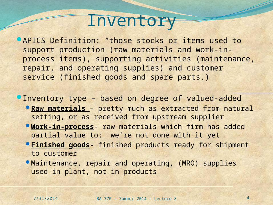
Inventory InvestmentBenefits of inventory

Provides buffer of materials/finished goods to resolve temporary demand/supply mismatches

Provides buffer for quality issues

Costs of inventoryConsumes working capital

Opportunity cost associated inventory, at costMust be physically maintained, stored, trackedPhysical deterioration

Shrinkage Obsolescence Aging, overaging


7

Inventory Measurements“At cost” for accounting purposes – dollar value of

inventory held based on cost, not valueInventory turns = COGS/Average Inventory

Comparative parameter: If one firm has a higher turns ratio, tends to have lower

inventory levels, reduced holding costs However the firm with the lower turns ratio may have

lower ordering/acquisition costs – may be benefiting from qty discount purchases

Inventory Age= Measurement period/Inventory turnsGives parametric measure of how long the average

item sits on the shelf…From cost point of view what is number large or small? What benefit comes from opposite?


8

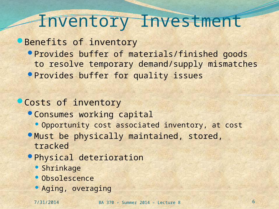
Inventory TypesTwo common elements:

Cycle Stock – most inventory – quantity ordered periodically and used periodically, traditional sawtooth level. Slope of line is usage per unit time.

Safety stock – Inventory held against variabilities in delivery/availability of materials. Normally expected not to be used.

0 10 20 30 40 50 60 70 80 900

200

400

600

800

1000

1200

InventorySafety Stock


9

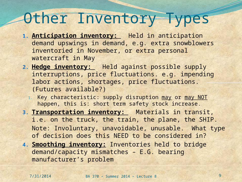
Other Inventory Types 1. Anticipation inventory: Held in anticipation

demand upswings in demand, e.g. extra snowblowers inventoried in November, or extra personal watercraft in May

2. Hedge inventory: Held against possible supply interruptions, price fluctuations. e.g. impending labor actions, shortages, price fluctuations. (Futures available?)

1. Key characteristic: supply disruption may or may NOT happen, this is: short term safety stock increase.

3. Transportation inventory: Materials in transit, i.e. on the truck, the train, the plane, the SHIP. Note: Involuntary, unavoidable, unusable. What type of decision does this NEED to be considered in?

4. Smoothing inventory: Inventories held to bridge demand/capacity mismatches – E.G. bearing manufacturer’s problem


10

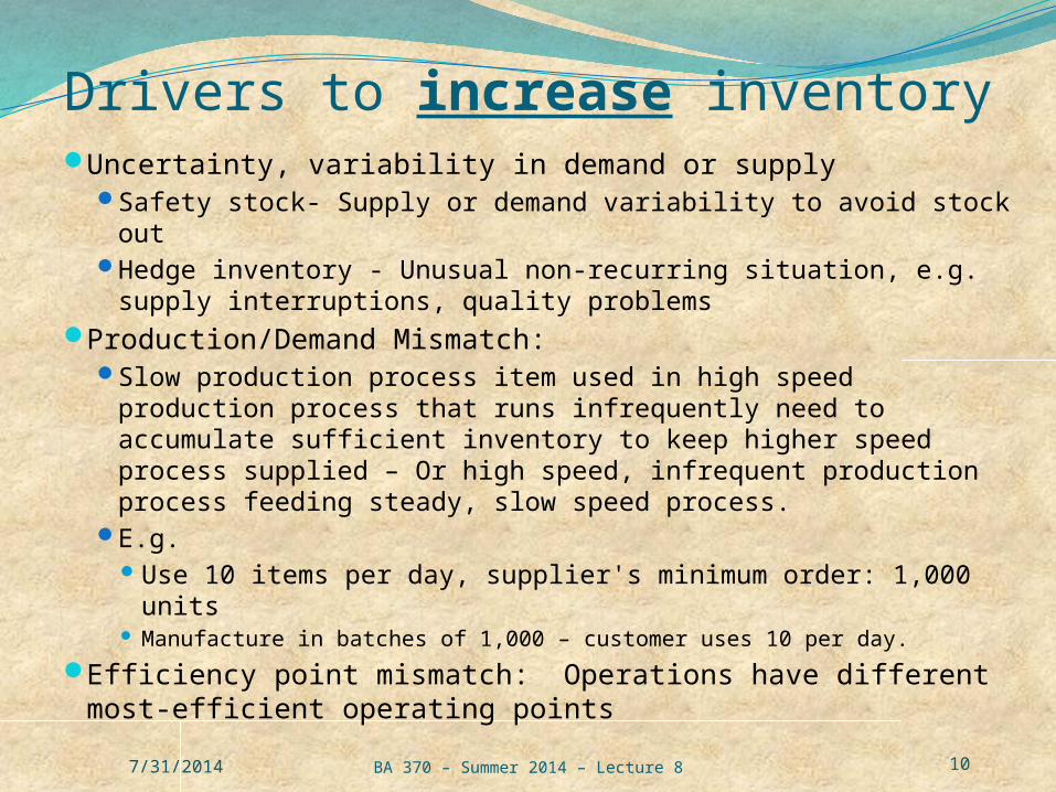
Drivers to increase inventoryUncertainty, variability in demand or supply

Safety stock- Supply or demand variability to avoid stock outHedge inventory - Unusual non-recurring situation, e.g.

supply interruptions, quality problemsProduction/Demand Mismatch:

Slow production process item used in high speed production process that runs infrequently need to accumulate sufficient inventory to keep higher speed process supplied – Or high speed, infrequent production process feeding steady, slow speed process.

E.g. Use 10 items per day, supplier's minimum order: 1,000

units Manufacture in batches of 1,000 – customer uses 10 per day.

Efficiency point mismatch: Operations have different most-efficient operating points

7/31/2014 BA 370 – Summer 2014 – Lecture 8

11

Drivers to reduce inventoryHolding costs:

Use of space, cost of physically maintainingShrinkage through theft, obsolescence, loss,

spoilageLiquidity; ties up cash – calculated as "cost of

capital"To identify operating problems – i.e. quality

problems often resolved by holding more inventory to prevent stoppages/stockouts due to quality problemsE.g. you have a supplier that ships products that

have a 25% reject rate: you need 100/day and keep two days’ inventory on hand – how many do you need to meet that requirement? 7/31/2014 BA 370 – Summer 2014 – Lecture 8

12

Demand DependenceIndependent demand: demand set outside

of firm’s control, usually final customer demand which you cannot control.

Dependent demand: Set within firm’s control, based on downstream demand Usually some component or sub-assembly,

maybe WIPIf the total demand schedule for finished goods

is set, the demand for individually produced components is determined by the specific requirements set by the product design


13

ABC Inventory AnalysisInventory ITEMS are ranked as to priority:

A Group- first, highest priorityB Group- first, middle priorityC Group- first, lowest priority

Rankings are based on item value, criticality, long lead time, annual usage value, shelf life

Simplest use is to set physical inventory counts frequency counts based on rank, higher priority gets counted more often


14

ABC Inventory MATRIX AnalysisConcept: Compare annual usage with current

inventory level, set based on ABC rankingsProcedure –

1. Establish annual usage cost ranking for item Find annual usage cost = Item unit cost x annual

usage, # Classify item based on annual usage cost

2. Establish current inventory value ranking for item Calculate item’s current inventory value = unit cost

x inventory # Calculate the total current inventory value Calculate item’s current inventory value % Classify item current inventory based on %

3. Analyze by comparing annual usage ranking value with current inventory level ranking


15

ABC Inventory Matrix Evaluation

Note: Item Usage numbers should be more stable than Current Inventory

What to do with SKU 286867703? What to do with SKU 2950632923?


16

ABC Inventory Matrix Analysis, Graphically

Method:Plot points for each itemDesired location for points, along 45° line


17

Inventory ManagementMost frequent question for inventory manager

Q1: When to order more? A1: Re-order point

Q2: How much to order? A2: Order quantity

Answers depend on:Demand?

How fast are we using it? Is usage rate constant or variable?

How much is in stock? How low are we willing to go? What happens if we stockout?

When can we get more? Is the lead time constant or variable?

How often do we check inventory? Continuously or periodically (once-in-a-while) ?


18

Monitoring Inventory: Two methods Basis: how often do we check inventory?Periodic Review Inventory System – inventory levels

monitored on fixed, periodic schedule.Periodic orders are issued based on 1. Replenishment time: how long before next shipment arrives2. Expected demand: how much is required before next

shipment

Continuous Review Inventory System – inventory levels monitored continuouslyThe moment inventory falls to allowable minimum level, more inventory is ordered

Which inventory monitoring method used drives the re-order/order quantity question.


19

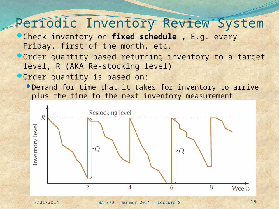
Periodic Inventory Review SystemCheck inventory on fixed schedule , E.g. every Friday,

first of the month, etc.Order quantity based returning inventory to a target level,

R (AKA Re-stocking level)Order quantity is based on:

Demand for time that it takes for inventory to arrive plus the time to the next inventory measurement


20

Periodic Inventory Review - Re-order Point

Known demand rate and lead time: Set R, re-stocking level at demand during lead time + review period

Eg. You check inventory every 7 daysIt takes 3 days to receive replacement inventoryYou use 50 units/day.

Set R, restocking level point at (3 + 7) x 50 = 500.

So, you are checking inventory and find 450 units in stock What is re-order quantity?Do you ever order 500 items?What will probably happen?What should we adjust and how?


inventory of at timeInventory

level restocking

quantityorder

:Where

I

R

Q

IRQ

INV_MODEL.xlsx

21

Periodic Inventory Review CalculationIf demand is not fixed, but normally distributed,

R can be set to give probability- based service level.


22

Calculating Service Level Service Level – A term used to indicate

the amount of demand to be met under conditions of demand and supply uncertainty. Assumes that the demand during the reorder

period and the lead time is normally distributed.


For a Critical Purchase – what should your inventory checking schedule be?

23

Continuous Inventory Review System Key features:

Constant monitoring of inventory levels

Set Re-order point: Replenishment order issued when inventory gets this low

Set Order quantity based on trade-off between holding costs and ordering costs, EOQ!

Reorder point based on Demand Supply Safety stock/ service levels

Note: For continuous review Re-order point is minimum inventory. For periodic review Re-order point is maximum inventory!!


24

Continuous Inventory Review System Assumptions:

Constant demand and lead time Holding and Ordering cost known and fixed Price of each unit is fixed

When Inventory gets to minimum point – called the Re-Order Point- an order is placed for more inventory. The order quantity, R is at least:

ROP = d X L Where: d = demand per unit time

L= lead time in units (that d is measured in.)What happens is this: When the inventory gets down to ROP,

ROP is ordered. During the time that it takes the new stock to arrive, the inventory falls to 0, just as R units arrive. Hopefully.


25

Continuous Inventory MonitoringDemand & Lead Time Variability

Continuous Re-order point

Variable demandNotice: L2≠L1, but L2>>L1Result: Either variability can cause stockout

Q

L1

RL2


Recall periodic Re-order pt!!

26

SRP: Probabilistic Demand & Constant Lead TimeRe-order point must cover

requirements caused by variable demand for the length of the fixed lead time.

So:

Z gives us the probability stocking out! This referred to as service level. So

at a 99% service level, what is z?

variancedemandDaily

timelead during demand Average

daysin timelead

:Where

d

d

d

LT

LTZdLTROP


27

SRP: Constant Demand & Probabilistic Lead TimeRe-order point must cover

requirements caused by fixed demand for the lead time’s variable length.

So:

Z refers to the service level. So if we want to have a 95% probability

of not stocking out, what Z do you use?

days variance, timeLead

timelead during demand Average

daysin timelead Average

:Where

LT

LT

d

TL

dZdTLROP


28

SRP –Probabilistic Demand & Lead Time

deviations standard ofnumber

time,lead ofdeviation standard

demand ofdeviation standard

periodsin time,lead average

period per time demand average d

:Where

222

Z

TL

dTLZLTdROP

LT

d

LTd


29

Reorder Points and Safety Stock When demand rate (d) and lead time (L) are

constant:

When demand rate (d) and lead time (L) or both varies:


30

Safety StockSafety stock:

= z x standard deviation of demand during the reorder period

=


31

Continuous Review Re-order point directs when to re-order to

avoid stocking out! Also gives minimum order amount based on replenishment time and demand.

But how much should you order? Just enough to get to bottom again? Maybe, maybe not!

Actually depends on costs/benefits of holding inventory!

Behold! The Economic Order Quantity model


32

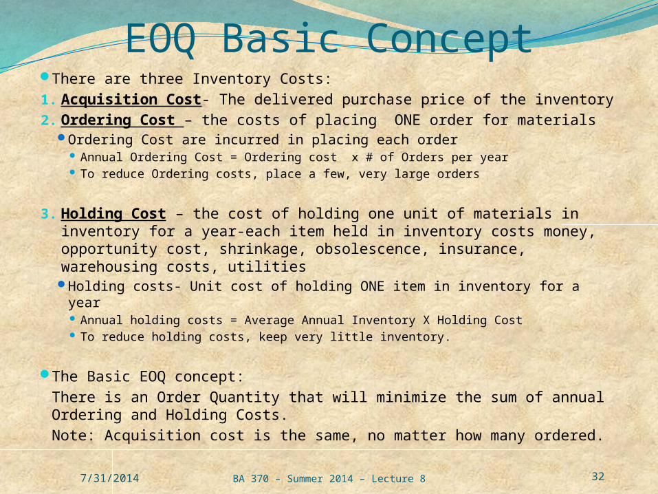
EOQ Basic ConceptThere are three Inventory Costs:1. Acquisition Cost- The delivered purchase price of the inventory2. Ordering Cost – the costs of placing ONE order for materials

Ordering Cost are incurred in placing each order Annual Ordering Cost = Ordering cost x # of Orders per year To reduce Ordering costs, place a few, very large orders

3. Holding Cost – the cost of holding one unit of materials in inventory for a year-each item held in inventory costs money, opportunity cost, shrinkage, obsolescence, insurance, warehousing costs, utilities

Holding costs- Unit cost of holding ONE item in inventory for a year Annual holding costs = Average Annual Inventory X Holding Cost To reduce holding costs, keep very little inventory.

The Basic EOQ concept:There is an Order Quantity that will minimize the sum of annual Ordering and Holding Costs. Note: Acquisition cost is the same, no matter how many ordered.


33

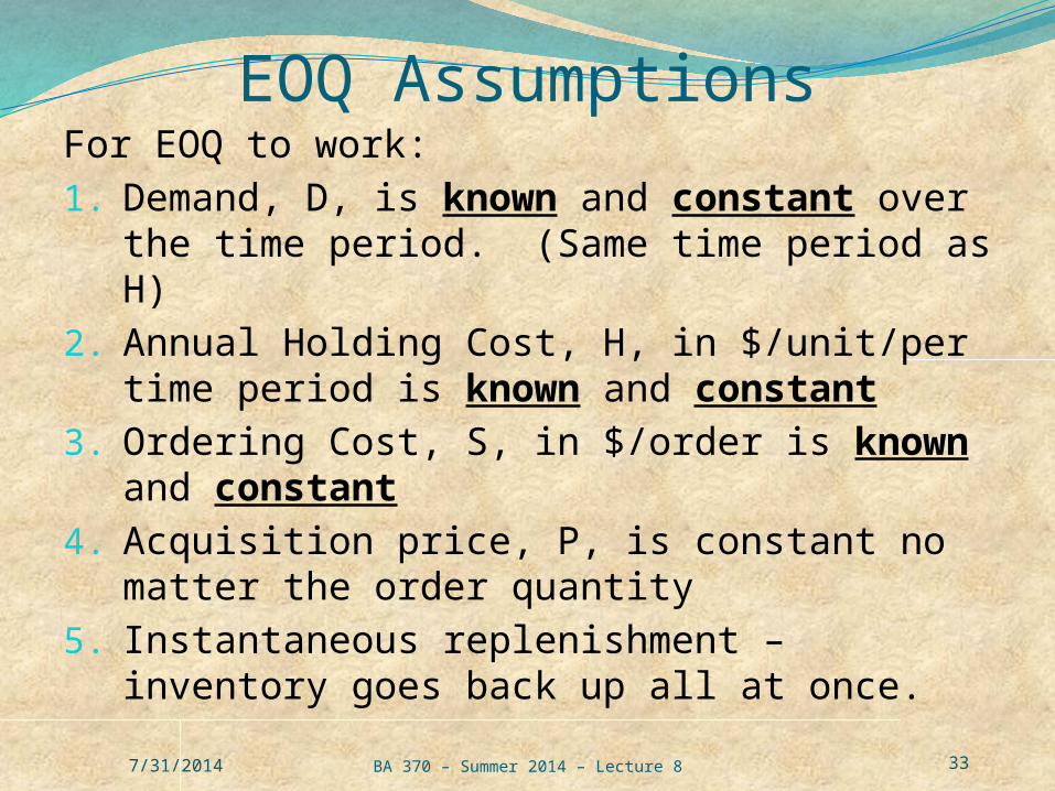
EOQ AssumptionsFor EOQ to work:1. Demand, D, is known and constant over

the time period. (Same time period as H) 2. Annual Holding Cost, H, in $/unit/per time

period is known and constant3. Ordering Cost, S, in $/order is known and

constant4. Acquisition price, P, is constant no matter

the order quantity5. Instantaneous replenishment – inventory

goes back up all at once.


34

EOQ – Common useage1. Time period, fixed. Usually 1 year.

2. Demand – Rate at which the inventory is used, in units per period . Must use same time period as holding cost period!

E.G. We use 500 sub-frames/month, annual demand is equal to 12 months X 500 = 6,000

3. Order Quantity, Q – Number of items ordered on one order


35

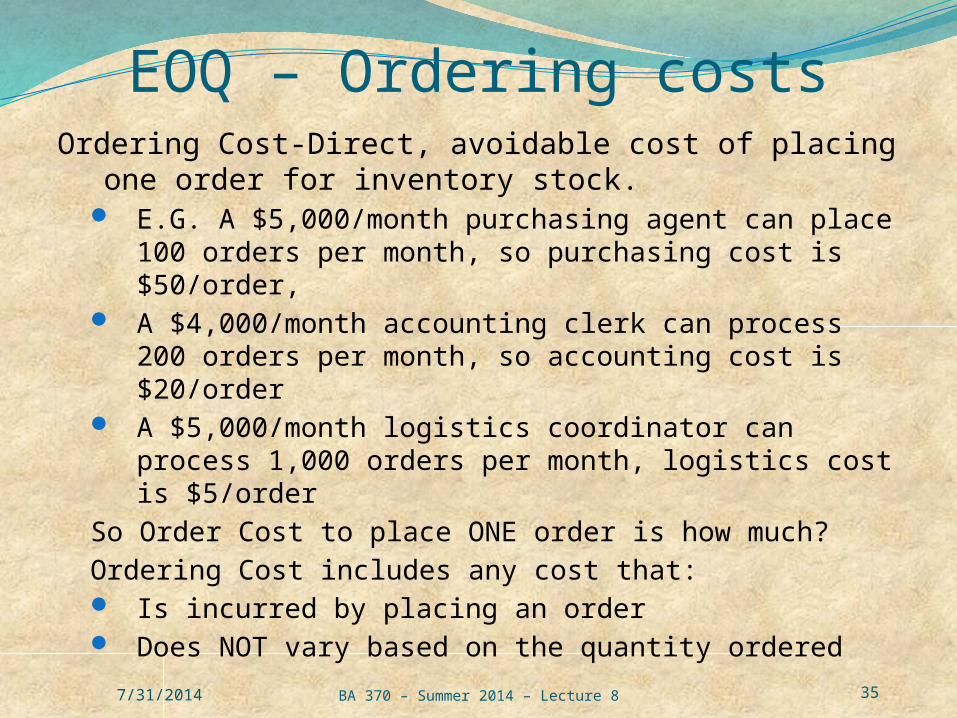
EOQ – Ordering costsOrdering Cost-Direct, avoidable cost of placing one

order for inventory stock. E.G. A $5,000/month purchasing agent can place

100 orders per month, so purchasing cost is $50/order,

A $4,000/month accounting clerk can process 200 orders per month, so accounting cost is $20/order

A $5,000/month logistics coordinator can process 1,000 orders per month, logistics cost is $5/order

So Order Cost to place ONE order is how much?Ordering Cost includes any cost that: Is incurred by placing an order Does NOT vary based on the quantity ordered


36

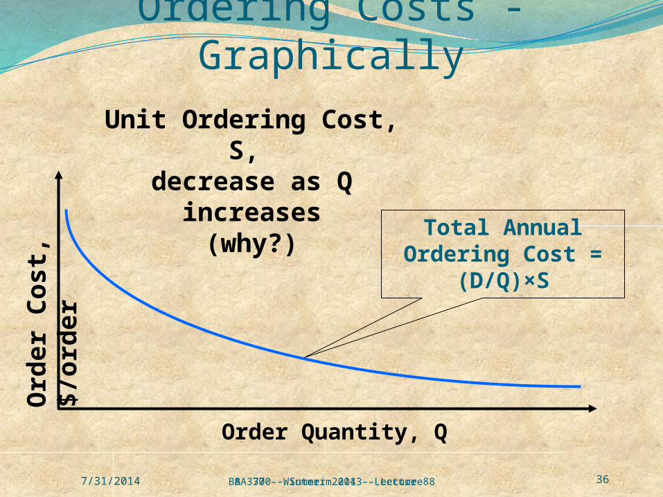
Ordering Costs - Graphically

Unit Ordering Cost, S, decrease as Q

increases(why?)

Total Annual Ordering Cost =

(D/Q)×S

Order Quantity, Q

Ord

er

Cost

, $/o

rder

BA 370 – Winterim 2013 – Lecture 8BA 370 – Summer 2014 – Lecture 87/31/2014

37

EOQ –Holding costsHolding Cost – Direct, avoidable cost of holding one item of

inventory stock for one year. E.G. Cost of capital is 10%, one subframe is worth $100,

opportunity holding cost is $100 X 10% = $10 Annual warehouse cost is $3.00/sq foot, a subframe takes

up 10 sq. ft. Warehousing Cost is $3.00/sf x 10 sf = $30.00 Annual Inventory shrinkage, obsolescence averages 10%

per yearShrinkage cost is 10% x $100 = $10 per year

So Holding Cost is how much?Holding Cost includes any cost that: is incurred by holding inventory is directly related to inventory quantity held increases through time

IT DOES NOT INCLUDE ACQUISITION COST!!! Why?


38

Average Inventory

2/fi QQI Recall EOQ Assumptions1. Constant Demand 2. Constant Order Quantity


39

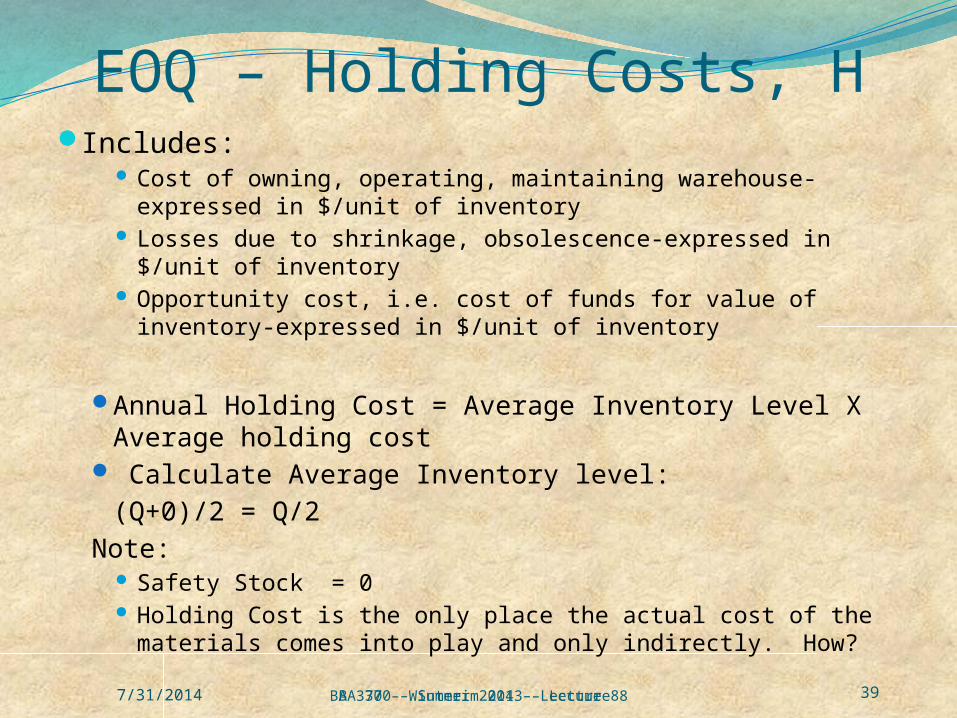
EOQ – Holding Costs, HIncludes:

Cost of owning, operating, maintaining warehouse-expressed in $/unit of inventory

Losses due to shrinkage, obsolescence-expressed in $/unit of inventory

Opportunity cost, i.e. cost of funds for value of inventory-expressed in $/unit of inventory

Annual Holding Cost = Average Inventory Level X Average holding cost

Calculate Average Inventory level:(Q+0)/2 = Q/2

Note: Safety Stock = 0 Holding Cost is the only place the actual cost of the

materials comes into play and only indirectly. How?BA 370 – Winterim 2013 – Lecture 8BA 370 – Summer 2014 – Lecture 87/31/2014

40

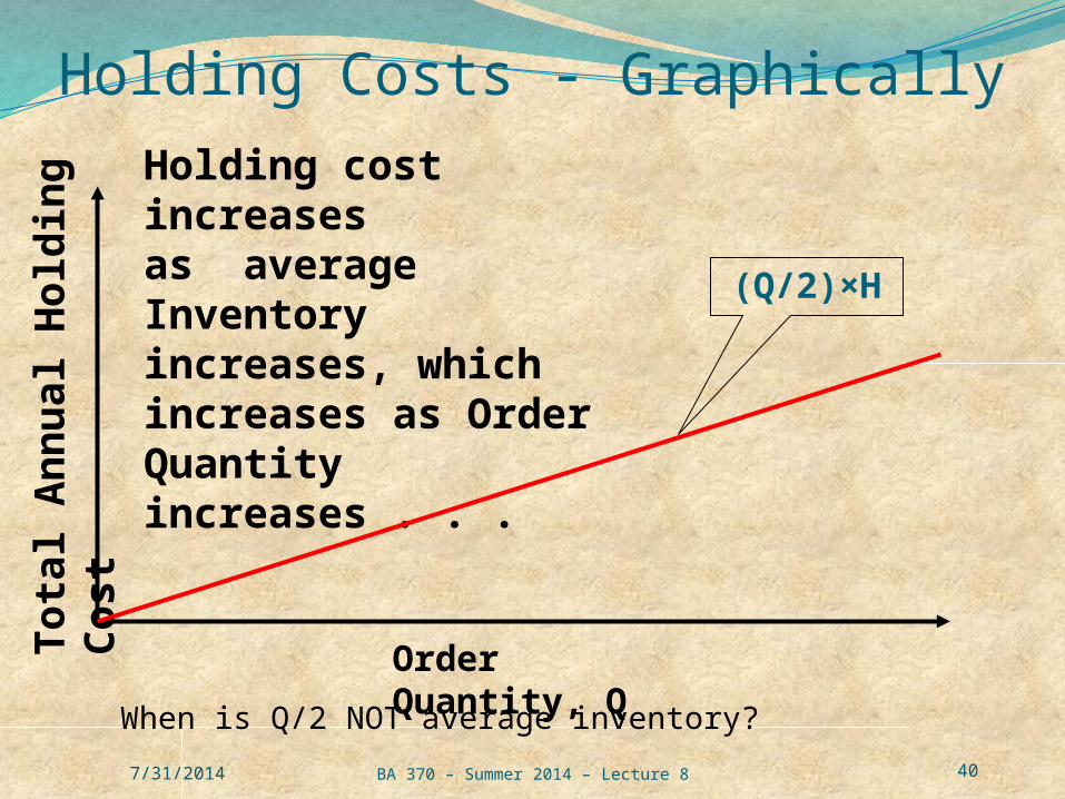
Holding Costs - Graphically

When is Q/2 NOT average inventory?

Tota

l A

nn

ual

Hold

ing

C

ost

Order Quantity, Q

Holding cost increasesas average Inventory increases, which increases as Order Quantity increases . . .

(Q/2)×H


41

EOQ Solution - Graphically

Ordering Costs, S, per year

decrease as Q increases

S, ordering costs

Order Quantity, QTota

l A

nn

ual

Ord

er

Cost

,$

Holding cost increasesas Q increases . . .

Total holding costs


42

EOQ Model – Tabular Procedure1. Plot the Order Cost Curve, Q vs $2. Plot the Holding Cost, Q vs $3. Plot the Total Cost = OC + HC4. Find Minimum Total Cost, min sum of total ordering and holding costs


43

EOQ – Direct Calculation

Cost OrderingS

Demand AnnualD

per UnitCost Holding Annual H

QuantityOrder Q

:Where

2

H

SDQ


44

EOQ Implications

Change Result

Increase DDecrease D

Increase SDecrease S

Increase HDecrease H

Increases EOQ, Average InventoryDecreases EOQ, Average Inventory

Increases EOQ, Average Inventory

Decreases EOQ, Average Inventory

Decreases EOQ, Average Inventory

Increases EOQ, Average Inventory

H

SDQ

2

Note: This tells us how much to order, not when to order.BA 370 – Winterim 2013 – Lecture 8

45

Example EOQ Ordering Costs – Graph

Total Annual Order Cost = S x (D/Q)


46

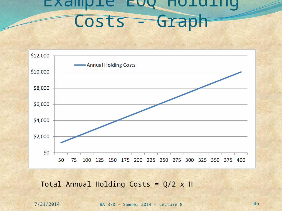
Example EOQ Holding Costs - Graph

Total Annual Holding Costs = Q/2 x H


47

Example EOQ Graph


48

Example EOQ - Graph

16.13450

7560002

Q What’s

wrong with this answer?


49

Example EOQ – Direct Calculation

The easy, more accurate way.

Useful if you are considering EOQ for range of products…


50

EOQ w/ Quantity DiscountSuppliers often offer lower unit prices for

larger order quantitiesEOQ model is based on assumption of fixed

pricesDiscount pricing can be accommodatedHow?

Recall: Basic idea of EOQ is finding minimum Total Cost for Holding and Ordering Costs

Method – Determine total purchase cost for various order quantities to identify lowest cost order quantity


51

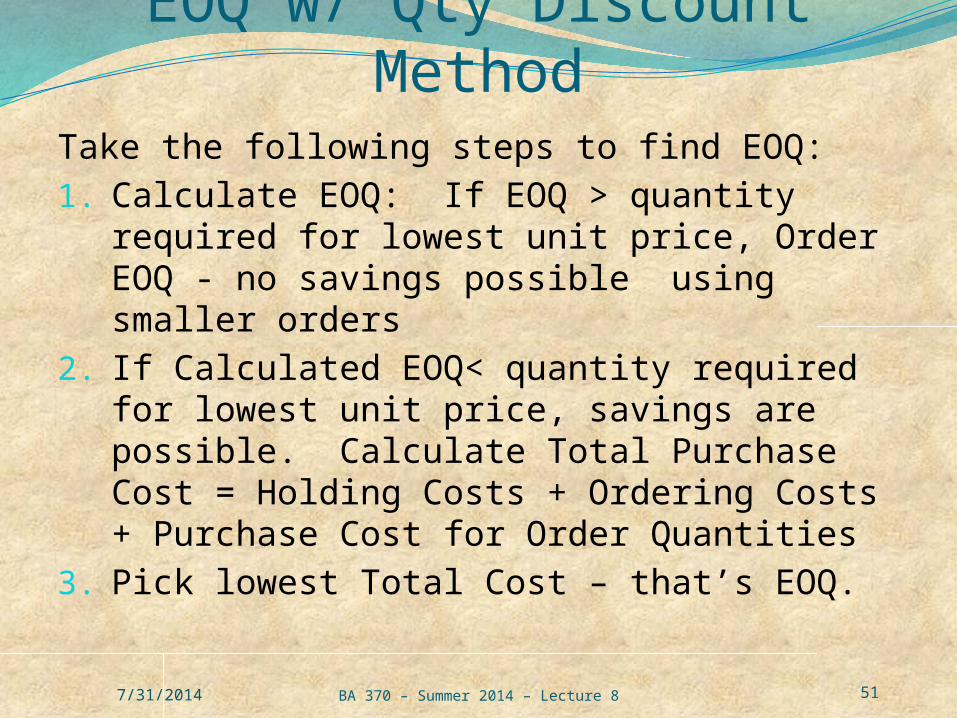
EOQ w/ Qty Discount MethodTake the following steps to find EOQ:1. Calculate EOQ: If EOQ > quantity required

for lowest unit price, Order EOQ - no savings possible using smaller orders

2. If Calculated EOQ< quantity required for lowest unit price, savings are possible. Calculate Total Purchase Cost = Holding Costs + Ordering Costs + Purchase Cost for Order Quantities

3. Pick lowest Total Cost – that’s EOQ.


52

EOQ w/Qty Discount Graphically


53

EOQ w/Price Breaks Example


54

Single Period InventoryAKA Newsboy Problem– Product only lasts a single

period Applies to inventory with short shelf life, just single

periodNewspapers Prepared foodsFish, fruitConcert ticketsSERVICES

Objective: How much to order? Economic considerations:

Stockout means :Lost sale, lost profit, maybe lost customerOverstock means: Loss of COGS, maybe disposal costsPeriod starting and ending inventory are always zeroObjective: Balance lost profits against unsold inventory cost


55

Newsboy - CostsShortage Cost

Cost of lost orders, based on lost gross profit or ‘contribution margin’

If item is component of a finished good, the contribution margin for the entire finished good is the cost of the lost

order

Overstock CostsCost of unsold inventory that must be disposed of or maybe salvaged If item is component of a finished good, only the costs for the item are included in the overstock costs

cost Item - price Itemcost Shortage Shortagec

cost Salvage -cost Disposal cost Itemcost Excess Excessc

56

Newsboy Procedure1. Determine Target Service Level, SLT based

on management input2. Determine Demand probability

characteristics3. Calculate Order Quantity, based on demand

probabilistic characteristics


57

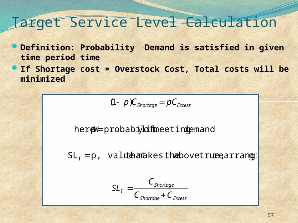
Target Service Level CalculationDefinition: Probability Demand is satisfied in given time

period timeIf Shortage cost = Overstock Cost, Total costs will be

minimized

ExcessShortage

ShortageT

ExcessShortage

CC

CSL

pCCp

grearrangin true,above themakes that valuep,SL

demand meeting ofy probabilitp here W

)1(

T


Find mean and variance of demandCalculate z value based on confidence levelCalculate Order Quantity Mean + zσ

Using Excel:

Target Service Level Calculation

59

Next lecture: 8/4 TuesdayOld BusinessWrap Up Inventory HW 3 due next ThursdayQuality ManagementBreakMore Quality


Summer 2014 Instructor: Daniel Hirsch, MBA, PE Lecture 8 July 31, 2014 Inventory Management.

Documents

Transcript of Summer 2014 Instructor: Daniel Hirsch, MBA, PE Lecture 8 July 31, 2014 Inventory Management.