ii

Summary Capital investment decision is one of the most important decisions, because it is thought to be affecting the short and long run situations of firms, and according to theory, it is thought to be affecting shareholders’ wealth. The researchers have recognized the two previously mentioned phases and conducted this study. This study aims at identifying the extent to which capital budgeting techniques and its related practices are used by Jordanian listed services firms, and identifying reasonable justifications behind that pattern of this use. The study also aims at identifying if there is any relationship between firms’ performance and the degree of capital budgeting sophistication. The researchers planned the study by formulating 3 research questions; these are, what are the capital budgeting techniques and their related practices that used by Jordanian listed services firms? Why Jordanian listed services firms use some capital budgeting techniques rather than others? What is the effect of the technique used on the firm’s performance? To answer these questions, the researcher developed a questionnaire and addressed it to the capital budgeting decision makers of Jordanian listed services firms. The sample of the study is the whole population; 63 Jordanian listed services firms. The researchers received back 38 usable replies after which they started their statistical analysis to reach at findings about their first two questions. As to the third question, the researchers used a multiple regression model that explains performance by the degree of sophistication and size of the firm. The researchers run the analysis for the multiple regression model on 30 firms, the firms that have their financial statements available at JSC. The results showed that PBP is the most used technique by the Jordanian listed services firms, followed by NPV, PI, ARR, and IRR. The results showed that the practices related to capital budgeting techniques; cost of capital estimation methods, risk analysis techniques, and cash flow forecasting techniques, are not widely used by the Jordanian listed services firms because of the domination of subjective judgment. When started their study, the researchers expected that the selection of the capital budgeting techniques is explained by demographical characteristics, type of capital investment decision, and\ or the perception of the respondents to the advantages and disadvantages of each technique. The results showed that academic qualification has a positive effect on the use of DCF techniques, while the type of capital investment decision has no effect on the capital budgeting techniques selection. Based on the respondents’ perception to the advantages and disadvantages of each technique, the advantages of PBP and NPV explain their high use, and the disadvantages of IRR explain its low use. Finally, the results of the multiple regression analysis indicate that there is no relationship between the degree of capital budgeting sophistication and the performance of the firms.

iii

Table of Contents

Chapter.1 Introduction

1.1 Background 1

1.2 Problem background 1

1.3 Gap in practice and theory 2

1.4 Statement of the problem 4

1.5 Purposes of the study 5

1.6 Scope and limitations of the study 5

1.7 Jordanian firms 6

1.8 Disposition of the study 6

Chapter No.2 Theoretical frame works and literature review

2.1 Introduction 8

2.2 Cash flow forecasting 10

2.3 Risk analysis 12

2.4 The discounting rate 13

2.5 Capital rationing 14

2.6 Capital budgeting techniques 14

2.6.1 Discounted cash flow techniques 15

2.6.2 Non-discounted cash flow techniques 17

2.7 Performance measure and the development of the measure 18

2.8 Previous studies 19

Chapter No.3 Methodology and methods

3.1 Choice of subject 26

3.2 Preconception 26

3.3 Perspective 27

3.4 Epistemology 27

3.5 Ontology 29

3.6 Scientific approach 29

3.7 Choice of methods 30

3.8 Population and sample of the study 31

3.9 Data resources 13

3.10 Research tools 32

3.10.1 The questionnaire 32

iv

3.10.2 The model 33

3.11 Statistical techniques used in the analysis 33

3.12 Variables of the study 33

3.13 Hypotheses of the study 34

Chapter.4 Observation and analysis

4.1 Description of the demographical characteristics of respondents 36

4.2 Degree of using capital budgeting techniques 37

4.3 The use of capital budgeting related practices 40

4.3.1 The use of cost of capital estimation techniques 40

4.3.2 Risk analysis techniques 41

4.3.3 Cash flow forecasting techniques 42

4.3.4 Comprehensive analysis for the capital budgeting related practices 43

4.4 Relationship between demographical characteristics and the use of techniques 43

4.4.1 Relationship between age and the use of techniques 44

4.4.2 Relationship between academic qualifications and the use of techniques 45

4.4.3 Relationship between experience and the use of techniques 47

4.5 Respondents’ perception to the advantages and disadvantages of the techniques 48

4.5.1 Respondents’ perception to the advantages of DCF techniques 49

4.5.2 Respondents’ perception to the disadvantages of DCF techniques 50

4.5.3 Respondents’ perception to the advantages of Non-DCF techniques 51

4.5.4 Respondents’ perception to the disadvantages of Non-DCF techniques 51

4.6 Relationship between the managers’ perception and degree of using the techniques 52

4.7 Relationship between capital budgeting sophistication and firm’s performance 54

Chapter.5 Conclusion and credibility criteria

5.1 Conclusion 58

5.2 Generalization 59

5.3 Validity and reliability 60

5.4 Implications 60

v

List of tables Table 1: Sub sector of services sector at ASE 6

Table 2: Previous studies 22

Table 3: Choices of philosophy and practical methods 31

Table 4: demographical characteristics of the respondents 36

Table 5: The degree of using capital budgeting techniques for replacement decisions 38

Table 6: The degree of using capital budgeting techniques for expansion decisions 39

Table 7: The degree of using capital budgeting techniques for lease or buy decisions 39

Table 8: The degree of using capital budgeting technique for independent projects 39

Table 9: The degree of using capital budgeting techniques for mutually exclusive 39

Table 10: The degree of using capital budgeting techniques for contingent projects 40

Table 11: The degree of using the techniques of cost of capital estimation 41

Table 12: The degree of using risk analysis techniques 42

Table 13: The degree of using cash flow forecasting techniques 42

Table 14: The degree of importance of the advantages of DCF techniques 49

Table 15: The degree of importance of the disadvantages of DCF techniques 50

Table 16: The degree of importance of advantages of Non-DCF techniques 51

Table 17: The degree of importance of disadvantages of Non DCF techniques 52

List of figures Figure 1. Relationship between age and degree of using capital budgeting techniques 44

Figure 2. Relationship between academic qualification and the degree of using capital budgeting techniques 46

Figure3. Relationship between experience and degree of using the techniques 47 Figure 4. Firm’s degree of sophistication 55

vi

List of appendixes

Appendix 1: The questionnaire

Appendix 2: Demographical characteristics of the sample

Appendix 3: Degree of using capital budgeting techniques

Appendix 4: Degree of using capital budgeting related practices

Appendix 5: Relationship between demographical characteristics and the degree of use

Appendix 6: Managers’ perception to the advantages and disadvantages of each technique

Appendix 7: The relationship between the perception of the respondents to the advantages

and disadvantages of the techniques and their use

Appendix 8: Multiple regression analysis

vii

Abbreviations

ARR: Accounting Rate of Return

ASE: Amman Stock Exchange

CBJ: Central Bank of Jordan

CEO: Chief Executive Officer

CFO: Chief Financial Officer

DCF: Discounted Cash Flow

IRR: Internal Rate of Return

Non- DCF: Non Discounted Cash Flow

NPV: Net Present Value

PBP: Pay Back Period

WACC: Weighted Average Cost of Capital

Abbreviations in tables

%: percentage

Cum %: cumulative percentage

Imp: important

L.imp: low importance

M.imp: moderate importance

m: mean

N.imp: not important

f: frequency

S.Dv: standard deviation

V.imp: very important

1

Chapter.1 Introduction This chapter identifies the problem, gap in theory and practice, the questions and the

purposes of the research, study’s limitations, a brief introduction about services firms listed

on Amman stock exchange, and the research disposition. The chapter introduces the reader

to a background that helps to understand the rest of the research.

1.1 Background Jordan is a small Arab country stands at the crossing point of Europe, Asia and Africa, enjoying a stable political and democratic environment (Amman Stock Exchange [ASE], 2010). Poverty, unemployment, inflation, and insufficient supplies of water, oil, and other natural resources are the fundamental economic problems in Jordan. King Abdullah II has become the head of the kingdom since 1999, and since that he has undertaken some broad economic reforms in a long-term effort to raise the living standards. Jordan's exports have increased under the free trade agreements with the US and Jordanian Qualifying Industrial Zones, these agreements allow Jordan to export goods with some Israeli content duty free to the U.S. In 2006 and 2008, Jordan used privatization to reduce its debt-to-gross domestic product ratio (Jordan country review, 2010, p. 59). In general King Abdullah II has been leading Jordan forward, and when it comes to the economic aspect, he is the one who initiated the reformation of more liberated and private directed economy and attracting billions worth investment into Jordan every year from the Gulf, Europe, and America (Country profile – Jordan, 2006, p. 5). Jordanian government, and as part of its 2002 Plan for Socioeconomic Transformation, has stressed its investments in health and education. This plan set economic, political, educational, and social welfare goals up to the year 2015. At the private sector level, several facilities have been granted to the education and health care investments (Country profile – Jordan, 2006, p. 9). The economic problems in Jordan make the investment climate of the businesses more challenging, and the researchers think that the plans and schemes set by the government and the king, if combined with a good firm’s strategy can help make the business planning and decision making more efficient.

1.2 Problem background Every firm has strategies to achieve, which might be developing a new product, exploring a new market, or beginning a new line of business. These types of strategies are reflected through what is called investments within the firm, and these investments have to be assessed to see if an investment will add value to the firm, and increase the shareholders wealth (Penman, 2010, p. 13). Adding value might take two aspects; maximization of accounting profit, and maximization of long term shareholders wealth. Good managers are concerned about the second aspect, since it is the one that has future prospects, reflects steady growth, and provide a risk shield, while accounting profit is a short term measure of the difference between the firm’s expenses and revenues (Arnold, 2008, p. 13).

2

When firms invest in their real assets or what is called capital investment, this involves allocating cash outflows for the purpose of receiving significant greater cash inflows; which means the expected future pay offs, over the useful life of the invested asset (Verma, Gupta, & Batra, 2009, p. 1) The expected pay offs involve future forecast, and this means inclusion of uncertainty or risk; ‘‘both words are used interchangeably to describe a situation where there is more than one possible outcome. Risk occurs when specific probabilities can be estimated to the possible outcome, while uncertainty applies in cases where it is not possible to assign probabilities’’, so the decision to be taken is a trade-off between the pay offs and the given risk (Arnold, 2008, p. 178). When assessing the investment projects, various capital budgeting techniques are used, while some practitioners prefer the non-discounted cash flow techniques, others use the sophisticated discounted ones. Though the non-discounted techniques used rigorously before, nowadays still mostly applied along with the discounted ones as a supplementary techniques (Verma et al., 2009, p. 1). Capital budgeting techniques are used to assess an independent single proposed investment project, or to choose the best project among some alternatives, given the cost, the expected return, and the associated risk. The preliminary assessment of the new projects has two possible outcomes, either the project is expected to generate more cash inflows and hence further assessing is needed, or cause more cash outflows and then rejected (Hilton, 2005, p. 676). According to Blocher, Stout, Cokins, & Chen (2008, p. 832), and Truong, Partington, & Peat (2008, p. 102), capital budgeting techniques are classified according to fact that some techniques consider the time value of money and then called discounted cash flow techniques, hence and after DCF techniques; the techniques under this category are:

• Net present value NPV • Internal rate of return IRR • Profitability index PI

While some other techniques do not consider the time value of money, and they are called the non-discounted cash flow techniques, hence and after Non-DCF techniques, and the most used ones are:

• Payback period PBP • Accounting rate of return ARR.

1.3 Gap in practice and theory Determining the best technique in evaluating the capital investment projects has been the concern of many researches and studies conducted by scholars and interested parties. Capital budgeting is one of the most important topics in the fields of the financial management, managerial accounting, and managerial economics, previous surveys have

3

showed how capital budgeting techniques are used in order to make crucial decisions, but different surveys conducted in the same or different times and applications, showed different results and findings. Mao (1970, p. 359), and Block (1997, p. 299) observed a preference for the non-discounted capital budgeting techniques especially the Payback period method. Lazaridis (2004, p. 432) conducted a study on Cypriot companies, and the results showed that 37% of the sample use the PBP, while the use of the DFC methods was as low as 11%, knowing that 19% of the sample do not use any of the capital budgeting techniques. Danielson & Scott (2006, p. 51) in their study concluded that most of the firms in their sample use the unsophisticated techniques, due in part to the limited educational background of some small business owners, small staff sizes, and liquidity concerns. Schall, Sundem, & Geijsbeck (1978, p. 286) observed an increasing trend towards the use of DFC methods especially IRR method, another study conducted by Haka, Gordon, & Pinches (1985, p. 667) concluded that using the DCF techniques have a positive effect on the firm’s performance on the short run, but there is no evidence of the long run effect. Pike (1996, p. 89) found that the gap between the theory and practice had decreased, since the firms adopting more sophisticated techniques. Jog, & Srivastava (1995, p. 43), Kester et al. (1999, p. 32), and Ryan, & Ryan (2002, p. 362) found the NPV, and the IRR to be the most used in Canada, the Asia-pacific region, and the U.S respectively. Verma et al. (2009, p. 14) concluded that there is an increased adoption to the NPV and IRR in corporate India, but still PBP is widely used, at least as a supplementary technique. In pure theory, and holding other related qualitative factors constant, the arguments are in the favor of the DCF techniques; Brealey, Myers, & Allen (2006, p. 103) consider the NPV technique the superior one, Arnold (2008, p. 77), Hirschey (2003, p. 622), and Bennouna, Meredith, & Marchant (2010, p. 226) argues that DCF techniques are preferred, because they require allowance for the opportunity cost of capital, and consider the time value of money when considering the maximization of stockholders wealth. Combining both theoretical assumptions and practical limitations, it is not as complex as the technique, as more accurate and rational as the investment decision. Some managers are either ignorant of the benefits of the DCF techniques, or facing some restrictions which hold them from the use. Good managers recognize that good investment decision is made according to different considerations within or outside the organization, and these considerations might be beyond the mathematical computation; financing considerations, social considerations, and\ or psychological considerations, but this does not mean to ignore the importance of the technique selection (Arnold, 2008, p. 144). The gap in practice and theory is not matter of identifying the superior techniques to be used, most of the practitioners and scholars know that DCF techniques make more rational and better evaluation, but the origin of the gap is what practitioners really use and what limitations hold them from using the DCF techniques (Williamson, 1996, p. 596).

4

1.4 Statement of the problem Looking at the gap in practice and in theory represented in the brief results of the previous studies and the theoretical assumptions, it is noticed that no agreed upon generalization can be made on the best technique to be used. So, the perception of the advantages and disadvantages of each technique, and the type of the investment are important factors when selecting the techniques to be used. The technique to be used in the evaluation process is one of the most important decisions in the capital budgeting process, knowing that each technique has its advantages and disadvantages. Some scholars and practitioners emphasize on the importance of the time value of money, cost opportunity of capital, and accuracy; represented by the DCF techniques, while others emphasize on simplicity, and liquidity concerns; represented by the Non-DCF techniques (Arnold, 2008, p. 72). For example, the PBP technique is still popular in the U.S when the projects evaluation is done by teams that include members with different experience and training; given the simplicity of the PBP and its easiness to understand teams use it. Another reason is that; American managers are known to be concerned about the short term profitability which is best measured by the PBP (Cooper, Morgan, Redman, & Smith, 2001, p. 19). But arguments against the cause of lacking experience can be opposed by the fact that mangers’ skills have been improved over time (Hermes, Smid, & Yao, 2007, p. 632). The researchers believe that each previous study is a special case and every new study tells something about capital budgeting practices at the time of conducting the study (Pike, 1996, p. 79), even when the techniques are not used in the capital investment process (Lazaridis, 2004). This leads to the fact that any new further study will bring a new insight into the use of the capital budgeting subject, given a different time and different application, from this point, this study is an analytical empirical study conducted on all listed Jordanian services firms, to give a new insight on the capital budgeting practices in Jordan. The researchers think that capital budgeting is a topic that needs to be analyzed in a very specific manners, where its practices are characterized and applied in a way that each application requires a specific practices; which means that the situation is the factor that determines the best practice to be applied. On other words management use discretion in judging the situation on hand, according to the financing issues, firm’ s industry, type of investment, and any other limitations and constraints. So, this study is conducted only on listed services firms, which have different types of capital investments comparing to other firms; like manufacturing firms or banks. The researchers believe that this kind of study can not achieve its objectives if it does not separate the firms according to the industry in which firms operate. Previous researchers have recognized this matter and conducted their studies on a base that consider the sector or the industry of the firms. In Jordan, Ramadan (1991), and Khamees, Al-Fayoumi, & Al-Thuneibat (2010) conducted capital budgeting studies on industrial firms, while Kester et al. (1999, p. 31), considered the industry differences a limitation on his study.

5

According to the knowledge of the researchers, this is the first study to be conducted on the services firms in Jordan. The findings and results of this study shall benefit many interested parties in the region and will give a new contribution to the practical field of the capital budgeting. The research questions are formulated as follow:

1. What are the capital budgeting techniques and their related practices used by Jordanian listed services firms?

2. Why Jordanian listed services firms use some capital budgeting techniques rather than others?

3. What is the effect of the technique used on the firm’s performance?

1.5 Purposes of the study The researchers set the first two purposes of the study as follow:

1. Explore the capital budgeting techniques and its related practices used by listed Jordanian services firms, and explore any relationship in the trend of the use to reasonable causes; demographical characteristics of the respondents, type of capital investment decision, and\ or the perceptions of the respondents to the advantages and disadvantages of each technique.

2. Assuming that the DCF techniques are the superior ones, where a firm is expected

to perform better when it applies the DCF techniques (Haka et al., 1985), and considering that the DCF techniques are consistent with the goal of maximizing a firm’s value (Bennouna, et al, 2010, p. 226), the second purpose is to: Find any relationship between the technique used and the performance of the firm.

Conducting this study on Jordanian firms is motivated by the researchers’ beliefs that Jordan is economically promising country, that is moving forward to a better investment environment. Jordanian government has done several economical leaps in order to be in a good competitive position: for example, attracting foreign investment through easier procedures and more privileges, adopting the schemes set by the international fund, and privatization, all to develop the Jordanian economy (Central Bank of Jordan [CBJ], 2010). The researchers believe that if the study achieves its objectives, it shall benefit the Jordanian practitioners of the capital budgeting techniques by directing them to the best technique to be used, and the ones that might result a better firm’s performance, if any relationship between the technique used and the performance of the firm exists. Academically, this research is an attempt to give a deeper insight on the use of the capital budgeting techniques, which might benefit the academic aspect of the capital budgeting field, as well as this study shall recommend more questions and further studies.

1.6 Scope and limitations of the study This study is conducted only on the listed services firms in Jordan, so the results and findings of the study can be addressed neither to other listed non services firms, nor to the

6

non listed services firms; the researchers exclude the non listed firms because of the positive relationship between the development of the financial markets and the use of the DCF techniques (Hermes, et al, 2007, p. 635).

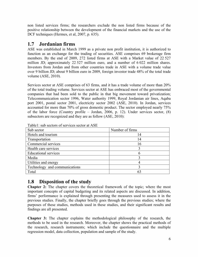
1.7 Jordanian firms ASE was established in March 1999 as a private non profit institution, it is authorized to function as an exchange for the trading of securities. ASE comprises 69 brokerage firm members. By the end of 2009, 272 listed firms at ASE with a Market value of 22 527 million JD; approximately 22 527 million euro, and a number of 6 022 million shares. Investors from Jordan and from other countries trade in ASE with a volume trade value over 9 billion JD; about 9 billion euro in 2009, foreign investor trade 48% of the total trade volume (ASE, 2010). Services sector at ASE comprises of 63 firms, and it has a trade volume of more than 20% of the total trading volume. Services sector at ASE has embraced most of the governmental companies that had been sold to the public in that big movement toward privatization; Telecommunication sector 1996, Water authority 1999, Royal Jordanian air lines, Aqaba port 2001, postal sector 2001, electricity sector 2002 (ASE, 2010). In Jordan, services accounted for more than 70% of gross domestic product. The sector employed nearly 75% of the labor force (Country profile – Jordan, 2006, p. 12). Under services sector, (8) subsectors are recognized and they are as follow (ASE, 2010): Table1: sub sectors of services sector at ASE Sub sector Number of firms Hotels and tourism 14 Transportation 14 Commercial services 16 Health care services 3 Educational services 6 Media 3 Utilities and energy 4 Technology and communications 3 Total 63

1.8 Disposition of the study Chapter 2: The chapter covers the theoretical framework of the topic; where the most important concepts of capital budgeting and its related aspects are discussed. In addition, firms’ performance is explained through presenting the measures used to assess it in the previous studies. Finally, the chapter briefly goes through the previous studies; where the purposes of these studies, methods used in these studies, and their significant results and findings are all presented. Chapter 3: The chapter explains the methodological philosophy of the research, the methods to be used in the research. Moreover, the chapter shows the practical methods of the research, research instruments; which include the questionnaire and the multiple regression model, data collection, population and sample of the study.

7

Chapter 4: The chapter includes both; the observation part and the analysis part of the study. The chapter starts with a description of the respondents and their trends in responding to the variables of the study, and then the analysis is made based on the data collected and statistical methods available by the SPSS. Chapter 5: The drawn conclusion from the observation and the analysis parts will be addressed in the chapter. Moreover, the creditability criteria will be discussed in the chapter.

8

Chapter.2 Theoretical frameworks and literature review This chapter covers the theoretical framework of the topic, it starts with a brief

introduction to the capital budgeting, then it explains the steps followed when making

capital investment decisions; cash flow forecasting, risk analysis, discount rate, capital

rationing, DCF techniques and Non-DCF techniques, and firms’ performance. According

the researchers’ beliefs, these are the most important relevant aspects of capital budgeting.

Finally, the chapter summarizes the most relevant previous studies conducted throughout

the past two decades.

2.1 Introduction Financial management has three main concerns; financing decisions, dividends decisions, and investment decisions. These decisions have developed in pursuing the overall goal of maximizing the wealth of shareholders. Financing decisions are the ones deal with the capital structure of the firm, while dividends decisions relate to the process of passing returns to the shareholders, and finally investments decisions have two forms; short term investments decisions, and long term investments decisions (Dayananda, Irons, Harrison, Herbohn, & Rowland, 2002, p. 1). Of the three aforementioned decisions, investment decisions have the greatest impact on firms (Eakins, 1999, p. 237). Capital budgeting is concerned with the long term investment, and their consistency with the overall goal of wealth maximization (Dayananda et al., 2002, p. 1). Capital budgeting decisions are among the most important decisions the firm has to take (Ryan, & Ryan, 2002, p. 355). Capital is the firm’s investment in fixed assets, while budget is a detailed plan of the expected cash flows (Hirschey, 2003, p. 607). Capital budgeting is the analytical process of planning and controlling the firm’s funds investment in capital assets (Cherry, 1970, p. 189). The importance of capital budgeting is derived from concept of maximizing the firm’s value because capital investment projects are supposed to maximize the value added to the stockholders (Hermes, et al., 2007, p. 632). The capital budgeting decision process involves large outlay fund, predicted inflows, long term commitment, and instability in the financial markets variables. Basically, financial markets variables include interest rate (Cooper, Morgan, Redman, & Smith, 2001, p. 1), inflation rate, foreign exchange, and the risk associated with the uncertain cash flow (Verma, et al., 2009, p. 9; Khamees, et al., 2010, p. 56). Different classifications are used in text books; the most known classification is (Ramadan, 1991, p. 188; Garrison, & Noreen, 1994, p. 650): • Replacement decisions: where the source of productivity is cost reducing. This kind of

investments was the most important decisions according to surveys conducted by Danielson & Scott (2006, p. 48)

• Expansion investment decisions: where the source of productivity is to generate more revenues by expanding the capacity of production and outlets. In this kind of investment decisions a new capital asset is acquired

• Mutually exclusive selection : where the decision is to choose one proposed project from several alternatives

9

• Lease or buy decision: should the capital asset be purchased, leased, or should the firm use outsourcing?

Some other factors can be referred to when classifying capital investment projects, such as the size of the investment outlay, risk and uncertainty of future cash flows, and patterns of cash flows (Khamees, et al., 2010, p. 50; Dobbins, & Pike, 1980, p. 13). The type of the investment could be an explaining factor in selecting the capital budgeting techniques and might lead managers to use some techniques rather than others (Bennouna, et al 2010, p. 231; Hermes et al., 2007, p. 637). According to Maccarrone (1996, p. 43) and Eakins (1999, p. 237), capital budgeting process has six phases or steps:

1. Identification of investment opportunity: where alternatives of projects are considered and must be formalized.

2. Evaluation and development: the process of analyzing the alternatives, where all available information is gathered. This phase includes costs-benefits analysis.

3. Selection: screening all investment proposals and considering the strategic and planning factors.

4. Authorization: this represents the management’s approval on the projects. 5. Implementation and control: this includes the carrying out and following-up

processes. 6. Post auditing: comparing outcomes to the budgets in order to have a feedback on the

whole capital budgeting process. The evaluation phase in the capital budgeting process involves collecting all information needed to reach at the optimal project, the one that maximizes the shareholders' wealth at most. The financial measure in the capital budgeting is the cash flows rather than the accounting profit, because the accounting profit and its accruals and realization concepts measure the result of the accounting process (Dobbins, & Pike, 1980, p. 19). In the selection phase, the firm ranks the refined proposed projects that have been evaluated, and accepts the projects according to the constraints (Eakins, 1999, p. 237). Three concepts surround the selection process, and these concepts classify the projects into three categories (Dayananda et al., 2002, p. 4):

• Independent projects: where the acceptance or rejection of the project does not affect the selection of other projects;

• Mutually exclusive projects: where the acceptance of a project eliminates all other projects; and

• Contingent projects: where the acceptance or rejection of a project is dependent on the acceptance or rejection of one or more other projects.

Management is concerned with accounting profit and other aspects like the market value of the firm, since the capital markets value firms according to their cash flows (Blocher, et al., 2008, p. 824). According to the theory of firm, profit maximization is the goal of any firm, but the new trend of this profit maximization concept has been evolved to a broad concept; maximizing the long term expected value (Hirschey, 2003, p. 5). Both concepts are related

10

to each other since the market share is highly correlated with the profits (Levy, & Sarnat, 1986, p. 11). Another factor is considered in the capital budgeting, that is; the timing of the cash flows which reflects the economic worth of the money (Blocher, et al., 2008, p. 824). Incorporating a value to the timing factor of the cash flows gives two categories classification for capital budgeting techniques, the first category considers the time value of money then called discounted cash flow techniques, while the other one ignores the value of cash flow timing (Dobbins, & Pike, 1980, p. 19).

2.2 Cash flow forecasting When assessing a capital investment project, cash flows of the project have to be predicted knowing that any new project will change the firm’s cash flows (Dayananda et al., 2002, p. 12). Cash flow forecasting is a critical step in capital investment assessing, because poor forecast results poor evaluation even if the best technique is used (Jog, & Srivastava, 1995, p. 39; Dayananda et al., 2002, p. 37). The accounting income is not the measure in the capital budgeting process; instead, the computation is made upon the cash flows of the project because accounting income is based on the accruals concept. Accrual concept ignores the timing of the cash flows (Garrison, & Noreen, 1994, p. 653), recognizes any expense or revenue that does not imply cash flow, and does not include the capital outlay in the computation (Hirschey, 2003, p. 610). Timing of cash flows is an important factor in the capital budgeting process, but the accounting income does not consider the timing of revenues and expenses (Garrison, & Noreen, 1994, p. 653). According to Blocher, et al. (2008, p. 825), cash flows in the capital investment projects involve cash outflows and cash inflows at three stages:

• Project initiation: in this stage most of the cash is flowing out; large funds outflows for initiating the project and supporting its operating expenses and a cash commitment is made to increase the net working capital.

• Project operation: in this stage, cash either flows in or costs are reduced as the investment generates benefits. More cash commitment supports the operations and additional increase is achieved in the net working capital.

• Project disposal: at the disposal of a project, cash inflows or outflows, moreover; the net working capital is released.

Incremental cash flow is an important concept of the evaluation phase in the capital budgeting. This is because the proposed project is supposed to maximize the market value of the firm through reflecting enough free cash flow (Mao, 1969, p. 185; Blocher, et al., 2008, p. 824). Thus, the only cash flows to be included in the evaluation are the incremental cash flows, which can be defined as the cash flows of the implemented project, mathematically (Arnold, 2008, p. 99): Incremental cash flows= firm’s cash flow with the project - firm’s cash flow without

the project

11

The proposed project has to be reformulated in terms of its expected net impact on the firm’s cash flows. This reformulation evaluates the effect of a given project on the firm, including its predicted effect on the firm’s value in the capital market (Cherry, 1970, p. 191).

Cash flows of a proposed project are the expected future cash inflows and outflows. Forecasting the outlays of the project is much easier than any other cash flows forecasting because its forecasting is in the near future. Thus, the further the forecasting goes into the future, the harder and more uncertain the forecasting is (Dayananda et al., 2002, p. 38). The firm has to identify the variables that affect the cash flows forecasting, and assess the variables that have the greatest influence on the forecasting process. The techniques used in forecasting the cash flows of a project are classified, as seen below, into two groups of techniques (Dayananda et al., 2002, p. 39): Quantitative techniques: they can be used when the past information about the variables is available and the information can be quantified. Quantitative techniques are:

• Forecasting with simple regression analysis: where the dependent variable is explained by one explanatory variable (Dayananda et al., 2002, p. 39).

• Forecasting with multiple regression analysis: where the dependent variable is explained by two or more explanatory variables (Dayananda et al., 2002, p. 42).

• Forecasting with time-trend projections: it is suitable for time series which exhibit a consistent trend over time, and the past trend is expected to continue in the future (Dayananda et al., 2002, p. 45).

• Smoothing models (or moving averages): these models are good for the near future forecast, where the average of last three or four observations are used for the next period (Dayananda et al., 2002, p. 46).

Qualitative techniques: they can be used when there is no past information, when the information can not be quantified, or when quantitative techniques need some judgment or subjective modifications (Dayananda et al., 2002, p. 55). Qualitative techniques are:

• Delphi method: eliciting estimates from experts within a group without allowing interactions between the members of the group (Dayananda et al., 2002, p. 61).

• Jury of executive opinion: it involves a meeting of the executives and deciding on the best estimate in the meeting (Dayananda et al., 2002, p. 61).

• Nominal group technique: a basic Delphi technique in a face to face meeting, which allows the discussion within the group (Dayananda et al., 2002, p. 63).

• Scenario projections: this describes expected hypothetical potential futures (Dayananda et al., 2002, p. 69).

Firms typically use quantitative techniques, and the management makes its own subjective estimate to the quantitative techniques. In most cases, the combinations of both techniques are applied by the firms. Given high uncertainty, firms need to choose cash flow techniques that allow them to manipulate and adjust the forecasting according to the risk characteristics (Jog, & Srivastava, 1995, p. 39; Hatfield, hill, & Horvath, 1998, p. 38).

12

Some practitioners criticize a given model, just because it does not give them the results they want, which means that they distrust the models especially when they do not want make an important decisions based on uncertain computations (Cooper et al., 2001, p. 16). Rules for estimating cash flows (Eakins, 1999, p. 262):

• Disregard sunk costs: the paid costs that can not be recovered, they are irrelevant because accepting or rejecting the project does not change them

• Include opportunity costs: which is the lost benefit as a result of choosing another alternative

• Adjust for taxes: because the tax effects might change the ranking of the projects • Ignore financing costs: because financing decision is separate from investment

decision and the DCF techniques already include the cost of funds • Adjust for inflation: by converting the nominal discount rate to a real discount rate

(Pike, & Neale, 2003, p.194) • Include indirect costs: ‘‘the cost that can’t be traced to the cost pool or cost object

(Blocher, et al., 2008, p. 56)’’.

2.3 Risk analysis Good estimation of project’s cash flows means less risk, because the total risk of a project is related to the overall uncertainty that is inherent to the project’s cash flows (Hull, 1986, p. 12). So, the estimation that fails to incorporate uncertainty and risk will almost give wrong choices and wrong conclusions (Brookfield, 1995, p. 56). Risk in capital budgeting is the degree to which cash flows are tending to be variable, or the chance that the project will prove unacceptable results; like generating negative NPV or generating a PI less than 1 (Gitman, 1987, p. 465). This occurs when there is an estimated probability for the possible outcome to differ from what had been forecasted (Arnold, 2008, p. 178). Basically firms use risk analysis to deal with the uncertainty in the projects’ cash flows (Jog, & Srivastava, 1995, p. 39). Types of risk (Pike, Neale, 2003, p. 281):

1. Business risk: the variability in cash flows which depends on the economic environment in which the firm operates

2. Financial risk: it results from the use of debt capital 3. Market risk: the variability in shareholders’ return

The risk associated with the cash flows of the project is measured by some developed techniques. According to Smith (1994, p. 20), these techniques are classified into either intuitive or analytical techniques. The former category of techniques gives a qualitative adjustment against the possibility of the difference between the expected cash flows and the future actual cash flows. Intuitive techniques are described by Jog, & Srivastava (1995, p. 39), & Smith (1994, p. 20) as subjective techniques. The latter techniques apply more quantification for the uncertainty surrounding the project.

13

The non-quantitative risk techniques or the so-called intuitive techniques are the following (Smith, 1994, p. 20):

1. Risk adjusted cash flows: by determining the level of cash flows that are believed to be received (Eakins, 1999, p.278)

2. Risk adjusted discount rate: where the discount rate is adjusted according to the riskiness of the project (Eakins, 1999, p.278). This technique is supported by the academic literature (Cooper et al., 2001, p. 18).

3. Subjective judgment 4. Risk adjusted payback period.

The techniques which apply the quantifications approach for risk analysis (Drury, 1996, p. 432) or what’s called analytical techniques (Smith, 1994, p. 20) are the following:

1. Sensitivity analysis: which considers the effects of changes in key variable one at time (Pike, & Neale, 2003, p. 291)

2. Simulation analysis: by considering all possible combinations of variables according to a pre-specified distribution (Pike, & Neale, 2003, p. 291)

3. Decision tree: mostly used when the problem involves a sequence of decisions, where an action taken at one stage depends on an action taken previously (Levy, & Sarnat, 1986, p. 288). This method presents all alternatives and payoffs and their probabilities (Gitman, 1987, p. 469)

4. Probability distribution: by measuring the risk of a project statistically through its cash flows (Gitman, 1987, p. 467)

To deal with uncertainty that surrounds cash flows, risk analysis techniques are used. The analytical techniques are sound and sophisticated, while the intuitive ones are subjective and less complicated. Managers use risk analysis techniques that give them a measure for the risk factor and can be adjusted according to their discretion (Jog, & Srivastava, 1995, p. 39). Mao (1970, p. 352) argued that firms need to choose portfolios rather than projects, and measure the risk by the variance of the returns or the cash flows, but this variance can be mathematically manipulated.

2.4 The discounting rate DCF techniques consider the time value of money, which means that the amount of cash flows at the moment differs in its value from the same amount to be received in the future. In finance terms, this is called the time value of money, and this concept is applied in DCF techniques by converting the cash flows into their respective values at the same point of time (Drury, 1996, p. 388). The DCF techniques apply the time value of money concept in order to obtain a superior measure of cost-benefit trade-off of proposed projects (Cooper et al., 2001, p. 15). The process of converting the expected cash flows into a value at the present time is called discounting, and this needs a discount rate to be used in the discounting (Drury, 1996, p. 388).

Discounting rate used in the capital budgeting is also called the cost of fund. Determining the cost of fund is the heart of the most capital budgeting rules (Chatrath, & Seiler, 1997, p. 21).Using a model that incorporates a single cost of fund; like cost of debt, or cost of equity, might lead to errors in the whole capital budgeting process. In theory, it is preferable that

14

weights base must be considered based on the capital structure of the firm when determining the discounting rate (Bennouna, et al., 2010, p. 229). Different models are used when determining the cost of capital. Academics and practitioners arguing for the superiority of the weighted average cost of capital (Ryan, & Ryan, 2002, p. 362; Bennouna, et al., p. 229). Other models incorporate the cost of borrowing either at banks or through issued bonds, cost of common stocks, cost of equity, and past experience. Firms use different discounting rates according to the investment nature and the financing terms (Lazaridis, 2004, p. 430). Cost of funds reflects the expected costs to finance the projects, the foregone earning power, and how the firm obtains funds now and then after. Moreover, cost of funds chooses the project with a rate of return that adds value to the firm, which means a rate of return above the cost of funds (Byers et al., 1997, p. 252). The discounting rate is adjusted to the related risk; high discounting rate is used for high risk projects whereas low rate used for less risky ones (Hirschey, 2003, p. 616). Theoretically and for an average risk project, the WACC is the appropriate discounting rate; otherwise an adjustment has to be done according to the given risk (Jog, & Srivastava, 1995, p. 40). Cooper et al. (2001, p. 15) suggest that the fluctuations in the interest rate have to be highly considered when adjusting the discounting rate because they are directly related. Obviously the study of Jog, & Srivastava (1995, p. 40) showed how far the practice is from theory when estimating the cost of capital.

2.5 Capital rationing Theoretically, firms should keep accepting more projects to the point where the marginal return equals the marginal cost, but limits on budget or borrowing make firms ration its funds to different investment (Kester et al., 1999, p. 30). Capital rationing occurs when there is a budget limit on the fund to be invested during a specific period of time. In this case, the firm has to decide on the best combination that yields the highest overall NPV (Schmidgall, 1995, p. 484). Two approaches are given to select projects under the capital rationing. The first approach is the IRR approach which applies the investment opportunity schedule by drawing the cost of capital line and imposing it to the budget constraints to determine the selected projects. The second approach is the NPV approach which is based on the concept of maximizing the wealth of the owners. In the second approach, the projects are ranked on the basis of their IRRs or PIs, and then PV of the benefits of each project is evaluated to determine the combination of projects with the highest overall PV (Gitman, 1987, p. 463).

2.6 Capital budgeting techniques In practice, there are five main capital budgeting techniques used when assessing investment projects. These techniques are the NPV, the IRR, the PI, the PBP, and the ARR (Ramadan, 1991, p. 89; Khamees, et al., 2010, p. 55; Cooper et al., 2001, p. 16). The arguments for the best techniques to be used are interesting to so many researchers. Every

15

study is concluding a different results and generalizations1. Theory suggests that NPV is the only value maximizing technique to be used in the selection process (Hatfield, et al., 1998, p. 38; Hermes et al., 2007, p. 632). Though the Non-DCF techniques are the least accurate ones, they are still nowadays used widely as supplementary tools (Hermes et al., 2007, p. 632). Yet the choice of the technique may be determined according to the individual preference and\ or the environment in which decision has to be made (Hermes et al., 2007, p. 635). According to Hermes (2007, p. 637), size of the firm, industry in which the firm operates, managers’ age, and managers’ education could be explaining factors of the choice of the capital budgeting techniques.

2.6.1 Discounted cash flow techniques The DCF techniques convert the predicted cash flows into their present values, which mean that these techniques consider the time value of money when assessing any capital investments projects (Blocher, et al., 2008, p. 834). The Net Present Value technique NPV

According to Blocher, et al. (2008, p. 836), the net present value of an investment is the difference between the present value of its cash inflows and the present value of its cash outflows. So, if a single proposed project generates a positive present value then the project is accepted, otherwise rejected, while the rule of decision to choose from different alternatives is to choose the one that generates the greatest NPV. The formula for the NPV technique is as follow: NPV= [(CFI 1/ (1+r) ^1) + (CFI 2/ (1+r) ^2) + ........... + (CFI n/ (1+r) ^n)] – CFO Where CFI: cash inflow r: the discounting rate 1, 2, n: number of the year CFO: initial cost (cash outflow)

Advantages of the NPV technique (Arnold, 2008, p. 72): • It considers the time value of money • It considers all cash flows during the life of the project • It assumes that the cash inflows are reinvested • It handles non conventional cash flows • It is consistent with the concept of maximizing the shareholders’ wealth (Drury, 2005, p.

235). Disadvantages of the NPV technique (Arnold, 2008, p. 72): • It does not give a percentage measure, only absolute amount, which does not help to

identify the best project among different sizes mutually exclusive alternatives • It assumes that the discounting rate is already known. • It does not consider the size of the investment (Cooper et al., 2001, p. 16)

1 See 1.3 Gap in practice and theory p. 2 of this study.

16

Internal Rate of Return IRR

IRR is the rate of return that produces a zero NPV, the rule of decision is to accept the project when its IRR exceeds the firm’s cost of capital (Blocher, et al, 2008, p. 837). Even though the cost of capital is not included in the IRR’s calculation, still it has to be compared to the calculated IRR. If the calculated IRR is greater than the cost of capital, then the project is accepted, otherwise it is rejected. The formula for the IRR is as follow (Blocher, et al., 2008, p. 837): IRR= (CFI 1/ (1+r) ^1) + (CFI 2/ (1+r) ^2) + ........... + (CFI n/ (1+r) ^n) Where CFI: the cash inflow r: the discounting rate 1, 2, n: number of the year

Advantages of the IRR technique (Arnold, 2008, p. 72): • It considers the time value of money • It considers all cash flows during the life of the project • It gives a percentage measure • It is consistent with the concept of increasing the firm’s value Disadvantages of the IRR technique (Arnold, 2008, p. 72): • It can not handle non conventional cash flows • Financing type decision may misinterpret the calculation result. • In mutually exclusive project, the IRR might incorrectly rank the projects (Drury, 2005,

p. 239). • It does not consider the size of the investment (Cooper et al., 2001, p. 16) Profitability Index PI

PI is known as the ratio of benefit\cost, this technique is derived from the NPV concept. The PI is computed by dividing the NPV of the proposed investment by the cash outflows of the investment. This technique overcomes one of the NPV’s pitfalls; that is, the disability to rank proposed investments on a percentage base rather than an absolute value base. Therefore, PI gives the ability to rank the investments according to their relative profitability (Williamson, 1996, p. 590). PI calculates the present value of benefit per unit currency of cost. The origin of the derivation of this technique comes from the decision rule of PI, where the independent project is accepted when it’s PI>1; this implies a positive NPV. Moreover PI’s decision rule for mutually exclusive projects is to choose the project with the highest profitability ratio. The formula of the PI is (Hirschey, 2003, p. 618): PI= PV of cash inflows\ PV of cash outflows Where: PV: present value

Advantages of the PI technique (Hirschey, 2003, p. 622): • It considers the time value of money

17

• It considers all cash flows during the life of the project • It gives a relative measure to rank projects according to their profitability Disadvantages of the PI technique (Arnold, 2008, p. 72): • It does not consider the size of the projects when it ranks them • It assumes that the discounting rate is already known.

2.6.2 Non discounted cash flow techniques Pay Back Period PBP

PBP of an investment is the time required for a project’s cash inflows to exactly equal the initial investment (Cooper, Morgan, Redman, & Smith, 2001, p. 16); or simply, is the period of time to recover the initial investment outlay. This technique is widely used, either as a supplementary one, or when the liquidity and recovery is the matter. The PBP is calculated by determining the time when the cash inflows recover the initial cash outflow. The formula for this technique is as follow (Blocher, et al., 2008, p. 842):

PBP= total initial investment/ annual cash inflow

Advantages of the PBP technique (Blocher, et al., 2008, p. 843): • The length of the PBP gives an indication about the risk factor, as more as the PBP, as

risky as the project • Easy to calculate and to understand Disadvantages of the PBP technique (Blocher, et al., 2008, p. 843): • It does not consider the time value of money • It does not consider the cash flows after the PBP • It does not reflect the profitability of the project. Accounting Rate of Return ARR

ARR of a project is the average accounting income of an investment as a percentage of the investment in the project, the formula for the ARR is as follow (Blocher, et al., 2008, p. 844): ARR= average yearly net operating income/ investment’s average

Advantages of the ARR technique: • It considers all incomes in the project’s life • Easy to calculate and understand Disadvantages of the ARR technique: • It ignores the time value of money • It ignores the cash inflows (considers the accounting income) • It ignores the lives of the projects (Arnold, & Panos, 2000, p. 485).

18

2.7 Performance measure and the development of the model Managers are supposed to do their best in pursuing the goal of maximizing the value of the firm. Stockholders are interested in this goal as well because it affects their returns. The return that stockholders are interested in is the accounting return and the capital return in the capital market (Hirschey, 2003, p. 7; Arnold, 2008, p. 13). At the academic level, theories have been developed to convince practitioners that the DCF techniques improve the capital budgeting decision process, but there is no evidence that using these techniques might result in a better performance (Farragher, Kleiman, & Sahu, 2001, p. 300). Different measures of performance have been used in previous related studies, Pike (1981) used the profitability and cash flows to measure the performance, Haka et al. (1985) used the market return as a performance measure, Agmon (1991) measured the performance based on the results of the financial statement, Ramadan (1991) measured the performance using different methods like return on investment, the return per share, and the market return of each firm, Farragher et al. (2001) used the operating rate of return, while Jiang, Chen, & Huang (2006) used the earnings as the performance measure.

The performance of the firms in this study is measured through a model that has been used by Farragher et al. (2001, p. 302). This model is a multiple regression model to examine the relationship between the performance and the degree of capital budgeting sophistication. In a study conducted by Klammer (1973, cited in Farragher 2001, p. 301), it was indicated that the degree of sophistication is represented by the use of the DCF techniques and incorporating risk in the analysis. The model is given by the following equation: OIROA j= b0+ b1ATj+ b2DCBSj Where: OIROA j= operating performance for firm j ATj= Size of firm j DCBSj= Degree of capital budgeting sophistication for firm j

OIROA j is defined as the operating rate of return for the firm j, where the operating rate of return equals operating cash flow divided by total assets.

ATj is defined as the total assets of firm j, and according to the model developed by Farragher et al. (2001, p. 302), the coefficient of this variable b1 is expected to be positive. DCBSj:

Where:

= Score for capital budgeting activity k for firm j

= weight assigned to capital budgeting activity k

19

=number of capital budgeting activities Given below are the activities incorporated in the performance measure of this study. It is worth-mentioning that ours are different from the ones used by Farragher et al. (2001, p. 310), but they include two of the ones used by Klammer’s (1973, cited in Farragher 2001, p. 301). Here in this study, the firm uses sophisticated practices if it uses the following activities:

1- Mainly use one of the DCF techniques. Hence and after a firm is considered mainly use a technique if it applies it either ‘‘Always’’, or ‘‘High use’’

2- Mainly use WACC to determine the discount rate 3- Mainly uses any of the analytical techniques in risk analysis

The score for each activity for every firm is measured on a scale of 0.0 to 1.0, where the firm gets 1.0 score if it conducts specific activity, and 0.0 if it does not. The weights are measured based on the respondents’ opinions about the degree of using each activity in the capital budgeting process. The weights are measured through a scale of 1 to 5, with 5 being the highest, and 1 being the lowest.

Where xi = 1, if the firm conduct the activity xi= 0, if the firm does not conduct the activity

2.8 Previous studies Capital budgeting decision makers have used various techniques to evaluate the proposed capital investment projects, and to determine the ones that benefit the firm the most. The adoption of particular techniques rather than others is determined by individual preferences, firm’s policy, and\ or the environment in which the decision has to be made. Every previous study claimed several factors as determinants of the choice of capital budgeting techniques (Hermes, et al, 2007, p. 635). In Jordan, Ramadan (1991) found an increasing trend toward adopting more sophisticated capital budgeting techniques by Jordanian Industrial Corporations when evaluating capital investment projects. Ramadan neither found a relationship between the techniques used and the performance of the firms, nor between the firm size and the techniques used. The sample of Ramadan’s study (1991) includes all listed Jordanian industrial corporations; 46 corporations. A questionnaire was addressed to the persons in charge of the capital budgeting decision, 37 usable replies have been analyzed to reach at the results of the study. Some corporations in Ramadan’s study (1991) refused to fill the questionnaire because they either claimed privacy issues, not having time, or tired of filling frequently flowing questionnaires. The questionnaire that Ramadan (1991) used, explored the techniques used by the respondents and some explanations for that use. NPV and PI were the most popular

20

techniques followed by the PBP, 30% of the firms use more than one technique. The managers use the DCF techniques because of their beliefs about the superiority of these techniques knowing that most of the managers are well educated and experienced. Moreover, firms are more adapting to the changes in the investment environment. The PBP is still used as a supplementary technique since it gives a good measure for the maturity of the project and because it is a good tool when the liquidity is the concern. Ramadan’s study (1991) showed that 50% of the corporations that apply DCF techniques use the borrowing cost as their discount rate since the projects in most cases are financed through debt. For risk analysis, 88% of the corporations use past experience and they use intuitive techniques when dealing with risk. When analyzing the relationship between the performance and the technique used, Ramadan (1991) found that on the long run there was no relationship between these variables, and to make his result more reliable he included the firms that use either the DCF techniques, or the Non-DCF ones, but not both. Ramadan (1991) used simple measures for the performance like Return on investment. Farragher et al (2001) studied the relationship between the use of sophisticated capital budgeting practices and corporate performance. The researchers developed a multiple regression model that explains the performance through some variables including the degree of capital budgeting sophistication. The data measuring the company’s degree of sophistication was gathered through a mailed questionnaire addressed to CFOs of 379 American industrial large companies, 34% returned questionnaire were usable replies. The analysis revealed that all variables included in the model except the degree of sophistication have their expected effects on the performance. The researchers expected that better performing companies use sophisticated capital budgeting practices, the results showed a negative relationship between performance and degree of capital budgeting sophistication. The results of Farragher et al.’s study (2001) are consistent with the results of Ramadan’s study (1991). In the Kingdom of Saudi Arabia, El-ebaishe, Karbhari, & Naser (2003) examined the use of selected management accounting techniques by medium and large sized Saudi manufacturing firms. A questionnaire was developed in line with previous researches, the questionnaire included 15 different management accounting techniques; capital budgeting is one of them. Before distributing the questionnaire, it was pretested through pilot interviews with 7 CFOs of the manufacturing companies. These pilot interviews helped in minimizing the wording ambiguity of the questionnaire and improving the relevance of its questions. The pilot interviews made the researchers exclude the small firms from their study after being uncertain about their responses. The results showed that vast majority of the surveyed companies use management accounting techniques employed by the study. Regarding Capital budgeting, 60% of the sample use capital budgeting when making capital investment decisions. Brounen, Jong, & Koedijk (2004) studied corporate finance in Europe. They examined the gap between theory and practice by measuring the extent to which theoretical concept are adopted by professionals. The researchers used a questionnaire developed by Graham, & Harvey (2002), which was awarded a Jensen Price in 2001. A sample of 313 European

21

CFOs answered the questions and the results showed that PBP technique is still used remarkably in Europe. The capital assets pricing model is the most used one to estimate the cost of equity. There is a positive relationship between the size of the firm on one hand and the use of DCF techniques and the capital assets pricing model on the other hand. Small firms and firms that are less oriented toward maximizing the shareholders wealth are more likely to apply PBP. These firms use whatever their investors tell them to use as cost of capital when applying DCF techniques. The education background of the respondents was irrelevant to the trend of using specific capital assets pricing model. The gap between theory and practice appears to be consistent across borders. The results of Brounen et al.’s study concerning capital budgeting was not significantly different from the results of the study conducted on the U.S firms by Graham, & Harvey (2002). The relationship between the capital expenditures and the corporate earning was the title of a study conducted on Tai corporations by Jiang et al. (2006). The study examined 357 manufacturing corporations listed on the Taiwan stock exchange. A sample period of 11 years was divided into capital investment period and performance period. The sample firms are grouped into eight portfolios ranked by capital investment ratio which is estimated from the investment period. The researchers examined the earnings in the performance period for the eight portfolios to see if any positive relationship exists. The results of Jiang et al.’s study (2006) showed a significant positive relationship between the performance of corporations in the sample and the capital expenditures. The study did not include the effect of the techniques used when making the capital expenditures, but it implicitly assumed the use of NPV technique. The most recent study conducted on Jordanian corporations provided empirical evidence on capital budgeting practices in Jordan, the study was conducted by Khamees et al. (2010). The researchers used a questionnaire and conducted interviews to collect the data of the study. Most of the 28 questions in the questionnaire were closed type questions, while the interviews were conducted before the distribution of the questionnaire. The interviews were conducted to clarify any ambiguity related to the questions in the questionnaire, to assure confidentiality to the respondents, and to show respondents the importance of their responses. The study targeted the industrial corporations and the questionnaires were addressed to 81 persons in charge of capital budgeting decisions in 81 corporations. The researchers received back 53 qualified questionnaires. The results of the study showed an equal importance of the discounted and non-discounted cash flow methods in evaluating capital investment projects. The most frequent used technique is the profitability index followed by the payback period. The results also showed that pitfalls in capital budgeting practices in Jordan are caused by the unfamiliarity with the techniques, misapplications of some adjustments like inflation, lack of staff and experience, and not using computer technology in evaluating capital investment projects. The researchers neither compare their results to the results of previous studies conducted on other countries, nor to the previous study conducted by Ramadan (1991). Khamees et al. (2010) claimed that their study is the first of its kind in Jordan. Khamees et al. (2010) found that PI technique followed by PBP is the most used technique. This result is similar to

22

Ramadan’s results (1991). The researchers found that cost of equity followed by cost of debt are the most used discounting rates, while Ramadan’s results showed cost of debt as the most used one. The following table shows previous related researches and surveys: Table 2: Previous studies

Title of the study Author- year- country

Purposes Research tool Findings

Sophisticated capital budgeting selection techniques and firm performance

Haka, Gordon, & Pinches (1985)

Explore the relationship between the firm performance and the use of capital budgeting techniques

Surveys and interviews

On the long run there was no relationship between the technique used and the performance of the firm, but there is a short run improvements in the return

Capital budgeting techniques and firm performance (Arabic article)

Ramadan (1991) Jordan

Explore the capital budgeting techniques used by manufacturing Jordanian corporations, and the relationship between the technique used and the performance of the firm

Statistical models and a questionnaire

An increased trend toward adopting the DCF techniques. And there is no relationship between the technique used and firm’s performance

An exploratory study into the adoption of capital budgeting techniques by agricultural cooperatives

White, Morgan, & Munilla (1997) U.S.A

Explore the utilization of capital budgeting techniques by agricultural cooperatives in strategic planning

Questionnaire and follow up contacts

DCF techniques are not used. The adoption of the DFC would improve the efficiency and effectiveness of the marketing and production needs

23

Title of the study Author- year- country

Purposes Research tool Findings

The association between the use of sophisticated capital budgeting practices and corporate performance

Farragher, Kleiman, & Sahu (2001)

Examine the relationship between the capital budgeting practice used and the performance of the firm

Multiple regression model on a sample of 117 firms

No relationship exist between the performance and the practice used

The theory practice gap in capital budgeting: evidence from the U.K

Arnold, & Hatzopoulos (2000) U.K

Explore the extent to which gap in theory and practice is trending

Literature review and survey

The practitioners of capital budgeting practices are more likely adopting the theoretical assumptions in their investment decisions

Capital budgeting practices of the 1000 fortune: how have things changed

Ryan, & Ryan (2002) U.S.A

Re-examine the capital budgeting methods used by the fortune 1000

Survey NPV and IRR are the most used techniques. As the size of investment increases, the adjustments concerns more likely to be considered

Corporate finance in Europe: confronting theory with practice

Brounen, Jong, & Koedijk (2004) Europe

Explore the extent of capital budgeting practices uses, address theory with the behavior of financial managers in practice

Literature review, and questionnaire

PBP is the most favored technique. firms that report that they maximize shareholder value are the same firms that prefer to use DCF

Capital expenditures and corporate earnings evidence from the Taiwan stock exchange

Jiang, Chen, & Huang (2006) Taiwan

Examine the relationship between capital expenditures and corporate earnings

Sample period is divided into capital investment period and performance period

Significantly positive association between capital expenditures and future corporate earnings, when accepting projects that generate positive NPV

24

Title of the study Author- year- country

Purposes Research tool Findings

Strategic investment decision making: the influence of pre-decision control mechanisms

Alkara,& Northcott (2007) Syria

Explore how pre-decision control mechanisms impact managerial decision making behavior regarding to strategic investment projects

Questionnaire and interview

Pre-decision controls, in a variety of forms, have a significant impact on how organizational actors view and evaluate strategic capital investment projects

Cost-of-capital estimation and capital budgeting practice in Australia

Truong, Partington, & Peat (2008) Australia

Analyze the capital budgeting practices of Australian listed companies

Questionnaire NPV, IRR and PBP are the most popular evaluation techniques. WACC and CAPM are mostly used for discounting

A survey of capital budgeting practices in corporate India

Verma, Gupta, & Batra (2009) India

Explore the capital budgeting practices in India particularly after the advent of full-fledged globalization and in the era of cutthroat competition

Survey Multiple techniques are applied for evaluation investments, PBP technique is used highly to supplement the DCF techniques. WAAC is the most used model in specifying the discounting rate

Capital budgeting practices in the Jordanian industrial corporations

Khamees, AlFayoumi,& AlThuneibat (2010) Jordan

Provide additional empirical evidence about capital budgeting practices in an emerging economy

Questionnaire and interviews

The results of the study show equal importance to the discounted and Non-DCF methods in evaluating capital investment projects. the most frequent used technique is the PI followed by the PBP

25

Title of the study Author- year- country

Purposes Research tool Findings

Improved capital budgeting decision making: evidence from Canada

Bennou-na, Meredit-h, & Marcha-nt (2010) Canada

Evaluate the use of capital budget techniques in decision making, and integrate the results with previous studies.

Survey Increase continuation in adopting DCF techniques

26

Chapter.3 Methodology and methods Methodology indicates to the whole approach to be used, including the underlying

philosophy and the rationale. Methodological considerations reflect the personal

preference of the researcher, while methods refer to the techniques to be used in the study.

Both terms are functions of the planning phase of a research (Johns, & Lee-Ross, 1998, p.

2). This chapter describes the methodology followed and the methods used in the study. The

theoretical and the practical aspects of the study’s methodology are explained as follow;

the choice of the subject, the preconceptions, the perspectives, the scientific approach, the

population and the sample of the study, instruments of the study, data collection, and the

statistical techniques used in testing and analyzing the hypotheses.

3.1 Choice of subject As we finished studying our core courses in accounting and chose to study finance as minor specialization, we started to think of a topic in both accounting and finance fields to be our thesis’s topic. Abdallah started the idea of writing about capital budgeting, since he had written about the topic in his previous degree; which was in finance. So, he discussed it with Yasir who found it a good idea because Yasir has enough background about the subject from the first core course he studied in Umea school of business; that is, value based management accounting. Capital budgeting is a crucial topic of financial management, management accounting, and managerial economics, and many theories have been developed to make the capital budgeting decision making more efficient and effective. In practice, so many researches have been conducted to explore the capital budgeting practices and to see how far the practice is away from the theory. The results of the researches were very interesting which made the authors more interested to write about the topic. The aspects of the study, its applications, and other related things have become clearer after meeting the thesis’s supervisor Åke Gabrielsson. The researchers took into account the supervisor’s comments about the topic in specific and the researches in general, and they were directed by his experience after which they reached the current specific title. It is worth mentioning that the changes in the structure and contents of the research continued throughout the process of writing.

3.2 Preconception We have been admitted to masters program in accounting in fall 2009, and we first met in the first core course; value base management accounting. We both came from almost the same cultural, social, and religious background; Yasir came from Iraq to Sweden in 2007, while Abdallah came from Jordan in 2009. Iraq and Jordan united for 3 years in the beginning of the sixties of this century. Both authors have the same mother tongue which makes communications between them easier. The work experience of both authors is a bit diversified, Yasir worked for the Iraqi government, American embassy in Iraq, and the telecommunication authority in Iraq. While Abdallah’s first job was a bookkeeper in his home town Irbid, then he moved to the U.S

27

where he worked 2 years in different kind of jobs. After that, he went back to Jordan to continue his graduate studies, and at the same time he started his job in the Jordanian income and sales tax department. Yasir has a bachelor degree in accounting from Iraq, while Abdallah has a bachelor degree in accounting and a master degree in finance from Yarmouk University in Jordan. Both authors have worked hard on formulating the problem and its description, and on covering the aspects of the study to make it clear to the readers. Suggestions and advice from our supervisor have been taken from the authors in a way that benefits them throughout the process of writing. Regarding the study questions, our first preconception is about the chosen sample, and we believe that there will be some relationships between the demographical characteristics of the sample and the use of capital budgeting technique; where we think that respondents whose ages are between 25 to 44, whose academic qualifications no less than master degree, professionally qualified, with work experience no less than 5 years, and\ or have some combinations of the previous factors, will be using more sophisticated capital budgeting practices. The second preconception is about the type of capital investment decision; where we think that when the respondents need to make capital investment decisions that involve generating more revenues; i.e., expansion decisions, they use more sophisticated capital budgeting practices than when they make cost reductions investment decisions, like replacement decisions and lease or buy decisions. We also think that respondents tend to use more sophisticated techniques when making mutually exclusive projects decisions and contingent projects decision, while less sophisticated techniques when making a dependent projects decision. We neither have preconceptions about the respondents’ perceptions of the advantages and disadvantages of each technique, nor about the relationship between the technique used and firms’ performance. But when we were reviewing the previous studies to develop a model that measures the relationship between performance and the degree of capital budgeting sophistication, an insignificant preconception of a positive relationship has been unintentionally obtained.

3.3 Perspective The applied perspective in this thesis is the point of view of the capital budgeting decision maker in the Jordanian listed services firms. The extent of using capital budgeting practices will be measured through the responses to the questionnaire’s questions. The demographical information of the respondents could be the explaining factor of the extent of use. The respondents will be the ones to determine this point of view, but the researchers have their expectations about this part which is represented in the hypotheses.

3.4 Epistemology Methodology is the comprehensive approach of a research, it represents the use of the methods, and it addresses the ontological and epistemological assumptions of the research.

28

Once the methods are chosen, the choice of reality happens; this choice includes deciding on the objects and issues in reality to be included or excluded in\ from the study. In addition, choosing certain methods; quantitative or qualitative affects the relations between the objects of the study. The decision on choosing objects, issues, and type of relations between them implies an ontological decision (Helve et al., 2005, p. 16). The nature of knowledge and how to be acquired has been a controversial issue; where rationalism sets reasoning to obtain knowledge and does not accept observation alone. In this kind of obtaining knowledge, power of logic is the factor that decides on the truth of theoretical argumentations, so the real truth is obtained through observation that is combined with reason (Ryan, Scapens, & Theobald, 1992, p. 5). The conclusion in the rationalism approach is reached through logic; drawing conclusion from set of facts or statements by using systematic set of rules. On the other hand, the other older way of acquiring knowledge is empiricism; where the observation is enough to build the truth upon it, but the modern empiricism has developed and accepted justification; where justification is necessary through an experience. So, the experience can represent a justification for our beliefs about what we know, which means that reasoning without an experience is meaningless (Ryan, Scapens, & Theobald, 1992, p. 5). The development of the empiricism has led to the most significant philosophical movements of thinking; positivism, which is considered to have strong influence on economics and accounting fields (Ryan et al., 1992, p. 6). Positivism implies that methodological procedures that applied on natural sciences can be applied on social sciences, and the results of the investigations can be formulated or expressed in terms of laws or generalizations (Cohen, Manion, & Morrison, 2000, p. 8). Measurement in positivism has to be objective and not to be a subject to any influence from the researcher side, this means that others can reach the same conclusions based on a given evidence, the precise measurement can be controlled by the researcher, and it allows statistical analysis to provide a precise answers. If the research’s design is formulated carefully, a causal relationship can be shown (Gratton, & Jones, 2004, p. 16). In this study, this is the approach to be adopted when measuring the relationship between the technique used and the performance of the study. According to Gratton, & Jones (2004, p. 16), positivism is an approach of objective investigation in which the researcher has no influence on the findings and the results, so, the most recognized characteristics of this approach are:

• The researcher controls one variable and evaluates its effect on the other variables • The same results occurs when repeating the experiment • Created hypotheses have to be tested

On the other hand, pragmatism’s claim on knowledge, emphasizes on the research problem rather than methods to be used, pragmatism concerns with the application ‘‘what works’’ and with the solutions to problems, and gives the researchers the option to use all methods for pursuing the solutions to the problems. Pragmatism means being free from any

29

commitment to any philosophy, being free to choose techniques or methods, not seeing the world as an absolute unity, and the truth is what works at the time (Creswell, 2003, p. 11). When the researchers started their research, and became more aware of the practical methods to be used in conducting the research, they thought that positivism is the most appropriate epistemology for this research because of the followings (Gratton, & Jones, 2004, p. 16):

• The researchers wanted the measurement to be objective and not influenced by the researchers; which is the concern of positivism

• It allows statistical analysis to provide a precise answer • Same results occurs when repeating the experiment

3.5 Ontology ‘‘Ontology refers to the philosophy of the existence and nature of phenomena (Gratton, & Jones, 2004, p. 15)’’. The nature of reality in social sciences can be divided into two types of ontological approaches; objectivism and subjectivism, if the researcher is investigating the phenomena as a reality that is not affected by one’s mind, then an objective approach is the followed one, but if the reality is affected by the individual to be included as part of the phenomena, then the subjective approach is the followed one. The controversial debate between these two approaches is known as the nominalism-realism debate (Cohen et al., 2000, p. 4). The researchers of this study chose objectivism ontology for the following reasons:

• The researchers wanted to investigate capital budgeting phenomenon as a reality that is not influenced by them.

• For the sake of pursuing objectivity. • The use of SPSS and the positivism epistemology. • Also the practical methods that the researchers planned to use played an important

role in determining the choice of philosophical view in perceiving and interpreting reality.

3.6 Deduction and Induction (Scientific approach) The two main approaches of a research are the deduction approach and the induction approach, and a combination of both approaches can be applied in a research. Deduction is reasoning a particular valid conclusion from a prior valid generalization (Cohen et al., 2000, p. 4). The hypothesis in the deduction approach is formulated in advance and then tested by the experiment to see if it is backed up by the practical experience, which means that the observation is made after the formulation of the hypothesis. The word ‘‘deduce’’ means to draw a conclusion from an assumption by reasoning (Johns, & Lee-Ross, 1998, p. 6). Induction approach stands for the opposite; reasoning a generalization from a prior valid specification. The observations made by the researcher should lead to a hypothesis; which means that facts are inducing the conclusion, simply the gathered data needs to be analyzed to extract hypotheses. The word ‘‘induce’’ means to lead to a conclusion (Johns, & Lee-Ross, 1998, p. 6).

30

In deductive approach, the hypotheses are formulated and developed to be tested through systematic sequences of logical steps to reach at findings to be generalized. In most cases this approach is associated with the quantitative data collection and analysis (Saunders, Lewis, & Thornhill, 2003, p. 86). While on the other opposite side, the sequence of the logical steps starts with data collection and analysis, and then reaches at findings that might be relied on to build theories upon; qualitative methods are the ones associate this kind approach (Saunders et al., 2003, p. 87). In many cases, it is not easy to take each of them as separate approach that needs to be applied in isolation, but it could be clear that a research is dominated by a specific approach (Cohen et al., 2000, p. 4). Finally, both approaches have the power of reasoning through sequence of formal steps of logic (Cohen et al., 2000, p. 4). According to Gratton & Jones (2004, p. 16), hypotheses have to be created and tested if the researcher is following positivism. Since the researchers of this study chose positivism, since the nature of the research questions imply hypotheses, and since the quantitative design is used, the researchers found that all those factors directing them to the deduction approach, as a matter of facts all the practical and philosophical methods explicitly indicate deduction.

3.7 Choice of methods The choice of method for any research should reflect the problem of the research (Bryman & Bell, 2003, p. 4). So, the researchers are considering their purposes when they test their hypotheses, and they are choosing the methods and approaches that fit their study sequence when pursuing the achievement of the purposes of the study. When using quantitative methods, the most significant strategies are the experiments and the surveys; the former includes the true experiments with the random assignment of subjects to treat the conditions, while the latter includes longitudinal and cross-sectional researches using questionnaire or structured interview to collect data, and makes generalizations from a sample to a population (Creswell, 2003, p. 13). After reviewing research methods in previous researches and in text books, the researchers have found that best method to fit this study is the positivistic epistemology that adopts deductive approach using quantitative methods to analyze the gathered data is the right way of analysis. These methods have been known as rule of thumb whenever a research involves a questionnaire or a developed model. For the first three questions of the study, the questionnaire will be the main data gathering tool, while a model will be used to answer the fourth question. The researchers are seeking ontological objectivity in conducting the research.

31

Table 3: choices of philosophy and practical methods of this study Epistemology Ontology Research

approach Research strategy

Time horizon Data collection

Rationalism Subjectivism Deduction Experiment Cross sectional

Interview

Empiricism Objectivism Induction Survey Longitudinal Questionnaire

Positivism Case study Secondary data

3.8 Population and sample of the study The population of the study comprises all Jordanian listed services firms; 63 services firms are listed at ASE. A questionnaire developed by the researchers has been addressed to the persons or the departments responsible for the capital budgeting decision (CEOs, CFOs, financial managers, or departments). The sample of the study is the whole population, and the choice of this decision is based on a rationale made by previous studies conducted in Jordan; Ramadan (1991, p. 195) and Khamees, Al-Fayoumi, & Al-Thuneibat (2010, p. 52). These previous researches studied manufacturing listed firms, and they chose the entire sector as their samples. Another justifications for choosing the entire population as a sample of the study is that the Jordanian listed services firms are divided into sub-sectors; where some of these sectors include 3-4 firms only. Therefore, the researchers tried to make the sample of the study more representative and comprehending to make more reliable generalization from the findings of the study. The justifications for choosing the listed firms only is briefly made because of some factors like the ability to measure the market performance of the firms, a belief that the listed firms are more willing to give information, and the fact that their financial statements are available on the web page of the Jordan securities commission. These financial statements will be referred to in order to collect some data for the model used in the performance analysis. Since the previous studies which were conducted on Jordanian firms studied the manufacturing firms, the researchers found an interest to explore a new application by conducting this study on services firms. In addition, some other reasons to conduct this study on Jordanian services listed firms are related to the motives previously mentioned in this study; ‘‘1.7 Jordanian firms, p. 6’’.

3.9 Data resources The data gathered for the study is one of two types:

• Primary resources: refer to the data that is gathered especially for the present research, this kind of data can be gathered through some special research tools such as a questionnaire or an interview (Gratton, & Jones, 2004, p. 8). The data gathered through these sources are to be used mainly in the empirical and the analysis part, and to test the hypotheses of the study. The primary source of data in this study is

32

the one gathered through the questionnaire which represents the point view of the respondents and answer the questions of the study.

• Secondary resources: refer to the data used in the study which is not its original

data, but it is an existing data from other previous studies or text books or other sources (Gratton, & Jones, 2004, p. 8). In this study, secondary data is represented by the literature review, books, surveys, and articles that relate to the topic. These kinds of data are either used to cover the theoretical frame work of the study and to set a comprehensive understanding of the topic, or they are represented by the previous studies. Previous studies set an overview of the topic in practice, and get the reader to understand the gap between theory and practice. Another secondary source is the financial data of the Jordanian listed services firms which answers the third question and finds any relationship between the performance of the firm and the use of the capital budgeting techniques. Most parts of this research contain an element of secondary data. Secondary data could be also used to support the primary data in the empirical and analysis part of the study.

For the purpose of collecting secondary data of this study, different books, databases, journals, and the Internet have been used. The databases that have been used are the ones available at the homepage of Umea University library (UB). Searches for sources have been conducted on EBSCO host.

3.10 Research tools To achieve the purposes of the study and to test its hypotheses, two tools are used; a questionnaire and a statistical model.

3.10.1 The questionnaire Contents and structure of the questionnaire The questionnaire comprises five parts:

• First part: it asks about the demographical characteristics of the respondents. These characteristics include age, academic qualifications, professional qualifications, and professional experiences. The first outcome to be reached when analyzing this part is to produce some observations about the capital budgeting decision makers of Jordanian services listed firms; this represents a descriptive outcome of the research.

• Second part: this part measures the extent to which capital budgeting techniques are used when taking an investment decision, where the use of the techniques is related to the type of investment decision. The choice of answers is based on a five-point Likert scale. In this scale, 5 ‘‘Always’’ represents the highest degree of use of the given technique, 4 ‘‘high use’’, 3 ‘‘moderate use’’, 2 ‘‘low use’’, and 1 represent the least degree of use ‘‘Seldom’’. Analyzing this part and producing some findings represents another descriptive aspect of the research.

• Third part: this part is designed to explore the managers’ perception of the importance of the advantages and disadvantages of each technique. The choice of answers is based on a five-point Likert scale. In this scale, 5 represents ‘‘very important’’ degree of the given advantage or disadvantage, 4 ‘’important’’, 3 ‘‘moderate importance’’, 2 ‘‘low importance’’, and 1 ‘‘not important’’. Analyzing

33

this part and producing findings represent another descriptive aspect. The findings are related to the extent of using some techniques rather than others, where managers’ perceptions of the advantages and disadvantages of each technique justify the extent of using the techniques.

• Forth part: this part is developed to explore the practices that used regarding the capital budgeting, where the respondents are asked about the extent of using each practice. The choice of answers is based on a five-point Likert scale. In this scale, 5 ‘‘Always’’; represents the highest degree of use of the given technique, 4 ‘‘high use’’, 3 ‘‘moderate use’’, 2 ‘‘low use’’, and 1 represent the least degree of use ‘‘Seldom’’. Analyzing this part and producing some findings represents a third descriptive aspect of the research.

3.10.2 Model A multiple regression model is used to identify any relationship between the techniques used and the performance of the study. The model was used before by Farragher et al. (2001, p. 302), but an elimination of some variables has been made to make the model more appropriate to the current study. The model used is given by the following equation:

OIROA j= b0+ b1ATj+ b2DCBSj

3.11 Statistical techniques used in the analysis The gathered data will be treated and analyzed through the statistical package for social sciences (SPSS). Different statistical techniques will be used according to the type of the data in hand as follows:

• Statistical descriptive methods: where the measures of central tendency will be used to describe the demographical characteristics of the sample, the degree of using capital budgeting techniques and other related practices and the respondents’ perception to the degree of importance to every advantage and disadvantage of each technique.

• Pearson correlation: it is used to find any correlation between some variables, one of them is dependent, where the other is independent. Pearson correlation measures the strength of the correlation at %95 of trust and a significance of %5.

• One way ANOVA test: it is used to find any significant statistical differences according to some categorization.

• Multiple linear regressions: it is used to find any relationship between more than two variables, one of them is dependent, where the others are independent.

• Chai- square test: it is used to explore the relationship between variables that take categorical form when they are coded.

3.12 Variables of the study Independent variables

• Demographical characteristics: include age, academic qualifications, professional qualifications, and experience. These variables are used in the third hypothesis, where the researchers check if there is any relationship connects them to the dependent variables; that is, the degree of using capital budgeting techniques. If

34

there is a relationship, it will be explained by the researchers. The data needed for this part is obtained by the primary data collection source; the questionnaire.

• Type of capital investment decision situations: include six types of capital investment decisions, where the researchers thought of a relationship between the type of capital investment decision and the degree of using capital budgeting techniques. The data needed for this part is obtained by the primary data collection source; the questionnaire.

• The perception of the advantages and disadvantages of capital budgeting techniques: where the researchers check if there is any relationship connects them to the dependent variable; that is, the degree of using capital budgeting techniques. If there is a relationship, it will be explained by the researchers. The data needed for this part is obtained by the primary data collection source; the questionnaire.

• The degree of capital budgeting sophistication: measured by some mathematical calculations that are developed by the researchers to see if this independent variables have any effect on the dependent variable; i.e. the operating performance of the firms. The data needed for this part is obtained by the primary data collection source; the questionnaire.

• size of the firm: measured by the total assets of each firm in the sample of the study to see if this independent variable has any effect on the dependent variable; i.e. the operating performance of the firms. The data needed for this part is obtained from the financial statement of the firms in 2009 as published on the web site of Jordan securities commission.

Dependent variables

• The degree of using capital budgeting techniques: this is expected to be explained by the demographical characteristics of the respondents, by the type of capital investment decision, and\ or by the perception of the respondents to the advantages and disadvantages of capital budgeting technique.

• Operating performance of the firms: which represents the dependent variable in the multiple regression model. It will be explained through the degree of capital budgeting sophistication and/ or the size of the firm.

3.13 Hypotheses of the study First hypothesis H0: Jordanian listed services firms do not use DCF capital budgeting techniques when assessing capital investment projects. H1: Jordanian listed services firms use DCF capital budgeting techniques when assessing capital investment projects. Second hypothesis H0: The type of the capital investment decision does not affect the degree of using capital budgeting techniques. H1: The type of the capital investment decision does affect the degree of using capital budgeting techniques.

35

Third hypothesis H0: Demographical characteristics of capital budgeting decision makers do not affect the degree of using capital budgeting techniques. H1: Demographical characteristics of capital budgeting decision makers do affect the degree of using capital budgeting techniques. Fourth hypothesis H0: Jordanian listed services firms do not use capital budgeting related practices when assessing capital investment projects. H1: Jordanian listed services firms use capital budgeting related practices when assessing capital investment projects. Fifth hypothesis H0: The perception of the respondents to the advantages and disadvantages of capital budgeting techniques is not the reason for the degree of using capital budgeting techniques. H1: perception of the respondents to the advantages and disadvantages of capital budgeting techniques is the reason for the degree of using capital budgeting techniques. Sixth hypothesis H0: firms with higher degree of capital budgeting sophistication do not perform better than firms with lower degree capital budgeting sophistication. H1: firms with higher degree of capital budgeting sophistication perform better than firms with lower degree capital budgeting sophistication.

36

Chapter.4 Observation and analysis The chapter includes both; the observation part and the analysis part of the study. The

chapter starts with description of the respondents and their trends in responding to the

variables of the study, and then the analysis is made based on the data collected and

statistical methods available by the SPSS.

4.1 The description of the demographical characteristics of the

respondents Table 4 shows the demographical characteristics of the respondents; it shows the age, the academic qualification, the professional qualification, and the experience of the people who responded to the questions of the questionnaire. The table shows the frequency, the percentage, cumulative percentage, mean, and standard deviation of each variable as follows: Table 4: demographical characteristics of the respondents Description\ (value) f % Cum % m S.Dv

Age 24 years or less (1) 2 5.3% 5.3% 25 – 34 years (2) 13 34.2% 39.5% 35 – 44 years (3) 12 31.6% 71.1% 45 years or more (4) 11 28.9% 100%

2.84 .916

Academic qualification

High school or below (1) 0 0% 0%

Community college(2) 6 15,8% 15,8% Bachelor degree (3) 21 55,3% 71.1% Master degree (4) 11 28,9% 100% P.HD degree (5) 0 0% 100%

3.13 .665

Professional qualification

None (1) 33 86.8% 86.8%

Certified Managerial Accountant (2)

1 2.6% 89.4%

Certified Financial Manager (3)

0 0% 89.4%

Jordanian Certified Public Accountant (4)

4 10.5% 100%

Certified Public Accountant (5)

0 0% 100%

Others (6) 0 0% 100%

1.34 .938

Experience 2 years or less 1 2,6% 2,6% 3 -12 years 12 31,6% 34.2%

13 – 22 years 14 36,8% 71.1%

23 years or more 11 28,9% 100%

2.92 .85

37

Referring to the table, we can notice that most of the capital budgeting decision makers in the sample of the study are middle aged, academic qualified, and experienced. 61% of the sample is 35 years old and more, 84% of them have at least a bachelor degree, and 66% of them have at least 13 years of experience. The respondents who have a professional qualification represent 13% of the sample; which means that most of the respondents have no such qualifications. Analyzing the given information above, we can say that most of the respondents have a good enough theoretical and practical skills in the field of the capital budgeting, and most likely they are supposed to be following the techniques that fit the firm’s capital investment decision and its related circumstances. The demographical characteristics of the current sample are almost similar to the demographical characteristics of Khamees et al’s sample (2010). From this point, we can say that the capital budgeting decision makers of services listed Jordanian firms have almost the same demographical characteristics of the capital budgeting decision makers of the industrial listed Jordanian firms. Based on the characteristics of the respondents, we can say that they are thought to know enough about the capital budgeting, and that the questionnaire had been addressed to the right people.

4.2 The degree of using capital budgeting techniques Since the nature of the study focuses on the use of capital budgeting techniques based on the type of the capital investment decision, the analysis takes place in the same manner.

Replacement decision The most used technique by Jordanian firms when making a replacement decision is the PBP; where the mean of using this technique by the sample scored the highest; 3.26, based on a 5 degrees scale. This mean means that the Jordanian firms use the PBP more than a moderate use. The percentage of the firms that use it either ‘‘Always’’ or ‘‘high use’’ is 58%. The researchers have set a criterion to measure the use of a specific technique or a practice as a main tool if the firm applies it either ‘‘Always’’ or ‘‘High use’’. So, hence and after, a main tool is the one used by the firm either ‘‘Always’’ or ‘‘High use’’. The PBP is followed by the NPV, the PI, and the ARR, and the means are 2.66, 2.34, and 2.13 respectively. These means mean that the Jordanian firms are using these techniques less than ‘‘moderate use’’ and more than ‘‘low use’’. While the percentages of firms that use these techniques either ‘‘Always’’ or ‘‘high use’’ were 34%, 26%, and 24% respectively. It is noticed that the IRR is the least used technique by the firms in the sample, where the mean and the percentage of using it as a main tool are the lowest. The mean of using the IRR is 1.58; which gives an indication of less than ‘‘Low use’’ application. Only 3% of the sample uses this technique as a main tool. In addition, the standard deviation of the IRR’s use was the least one; which gives more statistical confidence and more agreement by the respondents on the finding that it is the least used technique; where its standard deviation is 0.83. Table 5 shows the results of our analysis.

38

Table 5: the degree of using capital budgeting techniques for replacement decisions Seldom

(1) Low use

(2) Moderate

use (3) High use

(4) Always

(5)

f % f % f % f % f %

m S.Dv

NPV 14 37 9 24 2 5 2 5 11 29 2.66 1.70 IRR 21 55 14 37 2 5 0 0 1 3 1.58 0.83 PI 17 45 9 24 2 5 2 5 8 21 2.34 1.60 PBP 11 29 2 5 3 8 10 26 12 32 3.26 1.66 ARR 21 55 7 18 1 3 2 6 7 18 2.13 1.58 For the rest types of capital investment decisions, the same order of importance for the capital budgeting techniques is noticed when assessing capital investment projects. PBP is still the most used one with highest mean and percentage of use, followed by the NPV, the PI, and the ARR. For the IRR, it is also the least used technique. Very small minor differences in the means, the percentages of use, and standard deviations of each technique exist, but they are too small to be mentioned. These differences do not change the order of the degree of using the techniques. Based on the previous observation and analysis, the researchers reject the first null hypothesis; which states that ‘‘Jordanian listed services firms do not use DCF capital budgeting techniques when assessing capital investment projects’’. The researchers accept the alternative hypothesis; that is, ‘‘Jordanian listed services firms use DCF capital budgeting techniques when assessing capital investment projects’’. These findings are different than the ones of Khamees et al (2010), where they found that the industrial Jordanian firms equally use the DCF and Non-DCF techniques and the respondents in their sample showed an equal importance of the techniques. Our results showed that the firms use DCF techniques, but there is unequal importance of the degree of using the techniques because PBP is much more used than the second most used technique, NPV. While comparing our findings with the findings of Ramadan (1991) is a bit more consistent; the firms in his sample almost ranked the techniques in the same order that firms did in our sample except for the first two techniques. Moreover, in Ramdan’s sample the NPV is a little more used than the PBP. Because of this situation, the researchers presented only the tables that show the results of degree of using capital budgeting techniques considering the type of capital investment decision. These tables present the frequency, the percentage of the use, the mean, and standard deviation of each capital budgeting technique under each investment decision situation. This leads to an important initial finding; that is, the degree of using capital budgeting techniques is not affected by the type of capital investment decision. The tables that show the results of degree of using capital budgeting techniques according to the type of capital investment decision are as follows:

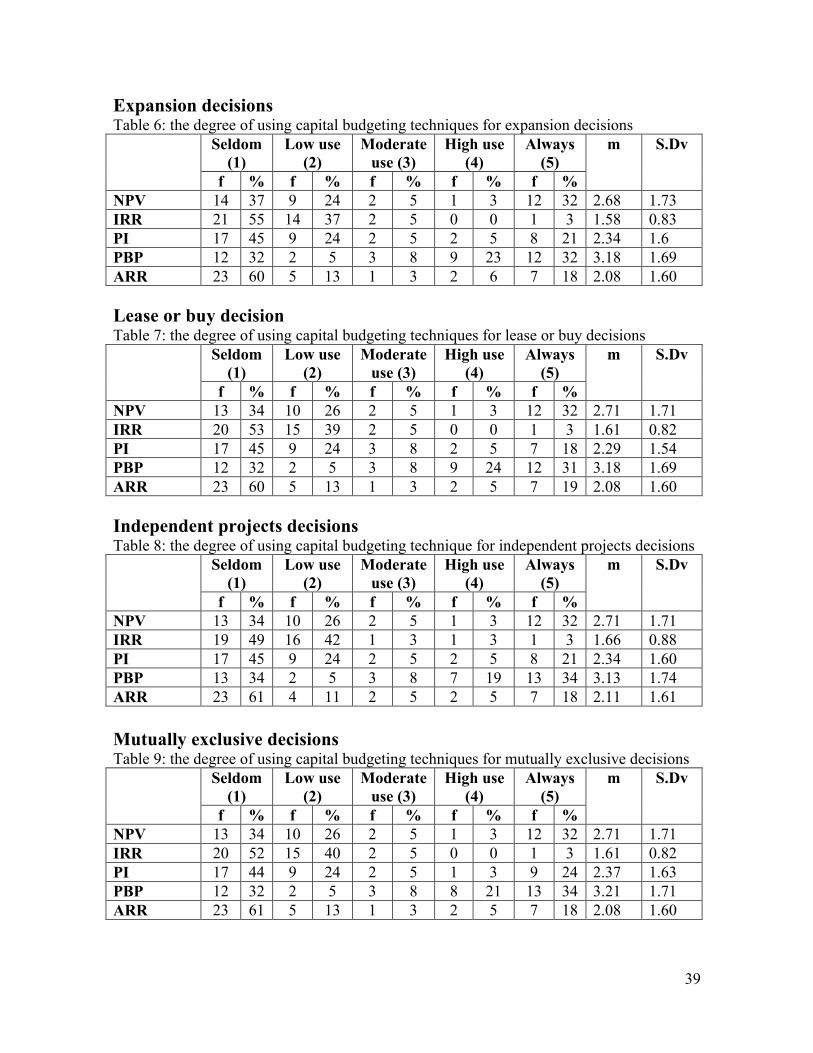
39

Expansion decisions Table 6: the degree of using capital budgeting techniques for expansion decisions

Seldom

(1) Low use

(2) Moderate

use (3) High use

(4) Always

(5)

f % f % f % f % f %

m S.Dv

NPV 14 37 9 24 2 5 1 3 12 32 2.68 1.73 IRR 21 55 14 37 2 5 0 0 1 3 1.58 0.83 PI 17 45 9 24 2 5 2 5 8 21 2.34 1.6 PBP 12 32 2 5 3 8 9 23 12 32 3.18 1.69 ARR 23 60 5 13 1 3 2 6 7 18 2.08 1.60

Lease or buy decision Table 7: the degree of using capital budgeting techniques for lease or buy decisions

Seldom

(1) Low use

(2) Moderate

use (3) High use

(4) Always

(5)

f % f % f % f % f %

m S.Dv

NPV 13 34 10 26 2 5 1 3 12 32 2.71 1.71 IRR 20 53 15 39 2 5 0 0 1 3 1.61 0.82 PI 17 45 9 24 3 8 2 5 7 18 2.29 1.54 PBP 12 32 2 5 3 8 9 24 12 31 3.18 1.69 ARR 23 60 5 13 1 3 2 5 7 19 2.08 1.60

Independent projects decisions Table 8: the degree of using capital budgeting technique for independent projects decisions

Seldom

(1) Low use

(2) Moderate

use (3) High use

(4) Always

(5)

f % f % f % f % f %

m S.Dv

NPV 13 34 10 26 2 5 1 3 12 32 2.71 1.71 IRR 19 49 16 42 1 3 1 3 1 3 1.66 0.88 PI 17 45 9 24 2 5 2 5 8 21 2.34 1.60 PBP 13 34 2 5 3 8 7 19 13 34 3.13 1.74 ARR 23 61 4 11 2 5 2 5 7 18 2.11 1.61

Mutually exclusive decisions Table 9: the degree of using capital budgeting techniques for mutually exclusive decisions

Seldom

(1) Low use

(2) Moderate

use (3) High use

(4) Always

(5)

f % f % f % f % f %

m S.Dv

NPV 13 34 10 26 2 5 1 3 12 32 2.71 1.71 IRR 20 52 15 40 2 5 0 0 1 3 1.61 0.82 PI 17 44 9 24 2 5 1 3 9 24 2.37 1.63 PBP 12 32 2 5 3 8 8 21 13 34 3.21 1.71 ARR 23 61 5 13 1 3 2 5 7 18 2.08 1.60

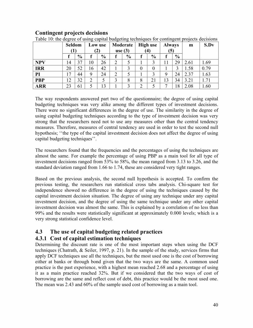
40

Contingent projects decisions Table 10: the degree of using capital budgeting techniques for contingent projects decisions

Seldom

(1) Low use

(2) Moderate

use (3) High use

(4) Always

(5)

f % f % f % f % f %

m S.Dv

NPV 14 37 10 26 2 5 1 3 11 29 2.61 1.69 IRR 20 52 16 42 1 3 0 0 1 3 1.58 0.79 PI 17 44 9 24 2 5 1 3 9 24 2.37 1.63 PBP 12 32 2 5 3 8 8 21 13 34 3.21 1.71 ARR 23 61 5 13 1 3 2 5 7 18 2.08 1.60

The way respondents answered part two of the questionnaire; the degree of using capital budgeting techniques was very alike among the different types of investment decisions. There were no significant differences in the degree of use. The similarity in the degree of using capital budgeting techniques according to the type of investment decision was very strong that the researchers need not to use any measures other than the central tendency measures. Therefore, measures of central tendency are used in order to test the second null hypothesis; ‘‘the type of the capital investment decision does not affect the degree of using capital budgeting techniques’’. The researchers found that the frequencies and the percentages of using the techniques are almost the same. For example the percentage of using PBP as a main tool for all type of investment decisions ranged from 53% to 58%, the mean ranged from 3.13 to 3.26, and the standard deviation ranged from 1.66 to 1.74, these are considered very tight ranges. Based on the previous analysis, the second null hypothesis is accepted. To confirm the previous testing, the researchers run statistical cross tabs analysis. Chi-square test for independence showed no difference in the degree of using the techniques caused by the capital investment decision situation. The degree of using any technique under any capital investment decision, and the degree of using the same technique under any other capital investment decision was almost the same. This is explained by a correlation of no less than 99% and the results were statistically significant at approximately 0.000 levels; which is a very strong statistical confidence level.

4.3 The use of capital budgeting related practices

4.3.1 Cost of capital estimation techniques Determining the discount rate is one of the most important steps when using the DCF techniques (Chatrath, & Seiler, 1997, p. 21). In the sample of the study, services firms that apply DCF techniques use all the techniques, but the most used one is the cost of borrowing either at banks or through bond given that the two ways are the same. A common used practice is the past experience, with a highest mean reached 2.68 and a percentage of using it as a main practice reached 32%. But if we considered that the two ways of cost of borrowing are the same and reflect cost of debt, this practice would be the most used one. The mean was 2.43 and 60% of the sample used cost of borrowing as a main tool.

41

The next followed techniques are cost of equity and cost of common stocks, with means of 2.32, and 2.26 respectively and the percentage of main use reached 21% each. While the least used technique is the WACC, and it is a special case since it is the most recommended technique by theory (Ryan, & Ryan, 2002, p. 362; Bennouna, et al., p. 229). The WACC scored the least mean and the least percentage of main use 2.18 and 20% respectively. These results are consistent with Ramadan’s (1991, p. 201), but different from the ones Khamees et al (2010, p. 56) had; where they found that cost of debt is used by only 30% of their sample. Table 11 shows the results of the statistical analysis of the use of the practices. Table 11: The degree of using the techniques of cost of capital estimation

Seldom

(1) Low use

(2) Moderate

use (3) High use

(4) Always

(5)

f % f % f % f % f %

m S.Dv

Weighted

average

cost of

capital

17 45 10 26 3 8 3 8 5 13 2.18 1.43

Cost of

borrowing

at banks

13 34 6 16 7 18 10 26 2 5 2.53 1.35

Cost of

borrowing

through

bonds

15 40 7 18 5 13 10 26 1 3 2.34 1.32

Cost of

common

stocks

16 42 5 13 9 24 7 18 1 3 2.26 1.27

Cost of

equity

16 42 4 11 10 26 6 16 2 5 2.32 1.32

Past

experience

10 26 8 21 8 21 8 21 4 11 2.68 1.36

4.3.2 Risk analysis techniques One important step in the capital budgeting process is risk analysis (Khamees, et al., 2010, p. 58). The results of the current study show that firms use risk adjusted PBP as the main practice for dealing with risk with a mean of 2.90 and a percentage of main use reached 50%. This makes sense to the researchers since the most used capital budgeting technique is the PBP. The next used practices are the subjective judgment and the risk adjusted discount rate; respectively their means were 2.84, 2.66. Their percentage of main use was 42% each. While the least used risk analysis practice was the decision tree, scoring the least mean, percentage, and standard deviation, they are respectively as follows; 1.53, 5%, and 0.98.

42

Table 12: The degree of using risk analysis techniques Seldom

(1) Low use

(2) Moderate

use (3) High use

(4) Always

(5)

f % f % f % f % f %

m S.Dv

Probability

distribution

17 44 6 16 3 8 6 16 6 16 2.42 1.57

Simulation

analysis

20 53 10 26 4 10 3 8 1 3 1.82 1.09

Decision tree 25 66 10 26 1 3 0 0 2 5 1.53 0.98 Sensitivity

analysis

21 54 6 16 4 11 3 8 4 11 2.03 1.40

Risk

adjusted

cash flows

15 40 5 13 8 21 10 26 0 0 2.34 1.26

Risk

adjusted

PBP

11 29 3 8 5 13 17 45 2 5 2.90 1.39

Risk

adjusted

discount

rate

14 37 3 8 5 13 14 37 2 5 2.66 1.44

Subjective

judgment

9 24 6 16 7 18 14 37 2 5 2.84 1.31

4.3.3 Cash flow forecasting techniques Cash flow forecasting practices are not mainly used by the Jordanian firms. The highest mean was 2.24; which indicates a less than moderate use, while for the rest of the techniques, the degree of use was even less than that, which indicates a low use. The most used techniques were simple regression, multiple regression, and jury of executive opinion, with a means of 2.24, 2.24, and 2.13 respectively. The percentages of using them moderately and above reached 39%, 39%, and 35% respectively. The least used technique is Delphi technique. The percentage of firms which use it moderately or more was 3%, the mean was 1.26 with a very low standard deviation of 0.5. This value of standard deviation gives a stronger agreement from the respondents’ side and more confidence on the mean. Table 13: The degree of using cash flow forecasting techniques

Seldom

(1) Low use

(2) Moderate

use (3) High use

(4) Always

(5)

f % f % f % f % f %

m S.Dv

Simple

regression

analysis

19 50 4 11 5 13 7 18 3 8 2,24 1,44

Multiple

regression

analysis

18 48 5 13 5 13 8 21 2 5 2,24 1,38

43

Seldom

(1) Low use

(2) Moderate

use (3) High use

(4) Always

(5)

f % f % f % f % f %

m S.Dv

Time-trend

projections

21 55 11 29 4 10 1 3 1 3 1,68 0,96

Moving

averages

25 66 8 21 4 10 0 0 1 3 1,53 0,89

Delphi

method

29 76 8 21 1 3 0 0 0 0 1,26 0,50

Nominal

group

technique

23 61 7 18 3 8 4 10 1 3 1,76 1,15

Jury of

executive

opinion

21 55 4 10 1 3 11 29 1 3 2,13 1,42

Scenario

projection

24 63 7 18 3 8 3 8 1 3 1,68 1,09

4.3.4 Comprehensive analysis for the practices used related to capital budgeting techniques All the related practices; cost of capital estimation practices, risk analysis practices, and cash flow forecasting practices, were used less than moderate use. The mean of the use was less than 3 for every single practice. In addition, whenever there is an option to use subjective judgment, it is the most used practice by the respondents, but the solid practices were the least used ones. The researchers based on the previous analysis conclude that the Jordanian services listed firms do not use capital budgeting related practices when assessing capital investment projects. Therefore, we can accept the fourth null hypothesis; ‘‘Jordanian listed services firms do not use capital budgeting related practices when assessing capital investment projects’’.

4.4 The relationship between the demographical characteristics and the

use of capital budgeting techniques To measure the relationship between the demographical characteristics and the degree of using capital budgeting techniques, the researchers excluded the professional qualification from the analysis because only 13% of the sample is professionally qualified. Also the analysis was run only on the relationship between demographical characteristics and the degree of using capital budgeting techniques for replacement investment decisions, and then it was addressed to all other investment decisions since. The reason for doing so is that, there was no difference in the use of the techniques according to the type of the investment decision. Pearson correlation is used to measure the relationship between the variables, and according to Pallant (2007, p. 132), the relationship has a small strength if it ranges from 0.10 to 0.29, a medium strength if it ranges from 0.30 to 0.49, and a large strength if it ranges from 0.50 to 1.00. There was nothing mentioned about the relationship that has strength less that 0.10, so the researchers assumed that this is a very small one.

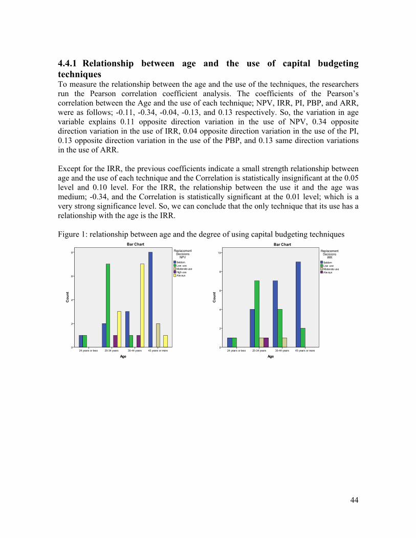
44

4.4.1 Relationship between age and the use of capital budgeting techniques To measure the relationship between the age and the use of the techniques, the researchers run the Pearson correlation coefficient analysis. The coefficients of the Pearson’s correlation between the Age and the use of each technique; NPV, IRR, PI, PBP, and ARR, were as follows; -0.11, -0.34, -0.04, -0.13, and 0.13 respectively. So, the variation in age variable explains 0.11 opposite direction variation in the use of NPV, 0.34 opposite direction variation in the use of IRR, 0.04 opposite direction variation in the use of the PI, 0.13 opposite direction variation in the use of the PBP, and 0.13 same direction variations in the use of ARR. Except for the IRR, the previous coefficients indicate a small strength relationship between age and the use of each technique and the Correlation is statistically insignificant at the 0.05 level and 0.10 level. For the IRR, the relationship between the use it and the age was medium; -0.34, and the Correlation is statistically significant at the 0.01 level; which is a very strong significance level. So, we can conclude that the only technique that its use has a relationship with the age is the IRR. Figure 1: relationship between age and the degree of using capital budgeting techniques

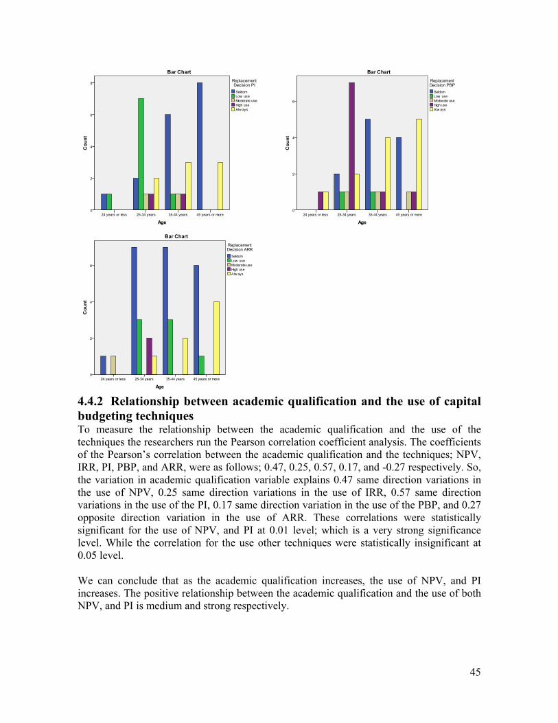
45

4.4.2 Relationship between academic qualification and the use of capital budgeting techniques To measure the relationship between the academic qualification and the use of the techniques the researchers run the Pearson correlation coefficient analysis. The coefficients of the Pearson’s correlation between the academic qualification and the techniques; NPV, IRR, PI, PBP, and ARR, were as follows; 0.47, 0.25, 0.57, 0.17, and -0.27 respectively. So, the variation in academic qualification variable explains 0.47 same direction variations in the use of NPV, 0.25 same direction variations in the use of IRR, 0.57 same direction variations in the use of the PI, 0.17 same direction variation in the use of the PBP, and 0.27 opposite direction variation in the use of ARR. These correlations were statistically significant for the use of NPV, and PI at 0.01 level; which is a very strong significance level. While the correlation for the use other techniques were statistically insignificant at 0.05 level. We can conclude that as the academic qualification increases, the use of NPV, and PI increases. The positive relationship between the academic qualification and the use of both NPV, and PI is medium and strong respectively.

46

Figure 2: relationship between academic qualification and the degree of using capital budgeting techniques

47

4.4.3 Relationship between experience and the use of capital budgeting techniques After running the Pearson correlation coefficient analysis, the coefficients of the Pearson’s correlation between the experience and the degree of using the techniques; NPV, IRR, PI, PBP, and ARR, were statistically insignificant neither at 0.05 level, nor at 0.10 level. So we can conclude that there was no relationship between the use of the techniques and the experience. Figure 3: relationship between experience and the degree of using capital budgeting techniques.

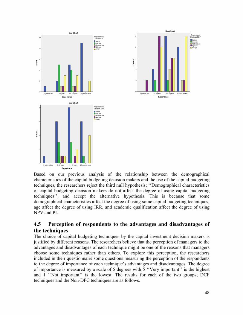
48

Based on our previous analysis of the relationship between the demographical characteristics of the capital budgeting decision makers and the use of the capital budgeting techniques, the researchers reject the third null hypothesis; ‘‘Demographical characteristics of capital budgeting decision makers do not affect the degree of using capital budgeting techniques’’, and accept the alternative hypothesis. This is because that some demographical characteristics affect the degree of using some capital budgeting techniques; age affect the degree of using IRR, and academic qualification affect the degree of using NPV and PI.

4.5 Perception of respondents to the advantages and disadvantages of

the techniques The choice of capital budgeting techniques by the capital investment decision makers is justified by different reasons. The researchers believe that the perception of managers to the advantages and disadvantages of each technique might be one of the reasons that managers choose some techniques rather than others. To explore this perception, the researchers included in their questionnaire some questions measuring the perception of the respondents to the degree of importance of each technique’s advantages and disadvantages. The degree of importance is measured by a scale of 5 degrees with 5 ‘‘Very important’’ is the highest and 1 ‘‘Not important’’ is the lowest. The results for each of the two groups; DCF techniques and the Non-DFC techniques are as follows.

49

4.5.1 Perception of respondents to the advantages of DCF techniques Most the respondents perceived the time value of money as the main advantage of the DCF techniques, the mean for this advantage scored the highest among all other advantages’ means. More than 50% of the respondents believe that time value of money is either an ‘‘Important’’ or ‘‘Very important’’ advantage of the DCF techniques. The second most important one is the consistency of DCF techniques with the concept of wealth maximization, with a mean of no less than 3.5, and a percentage of no less than 45% of respondents who believed that this advantage is an important one. The advantage that most of the respondent found it the least important one is the ability of IRR and PI to give a percentage measure, this advantage score the least mean and only 35% of the respondents found it an important advantage. In general all the advantages of DCF techniques are perceived as important by the respondents with a mean ranges from 3.2 to 3.9, and a percentage of agreement; considering them either ‘‘Important’’ or ‘‘Very important’’, ranges from 34% to 58%. This leads to a conclusion that capital budgeting decision makers of Jordanian listed services firms believe that the advantages of DCF techniques are important. Table 14: The degree of importance of the advantages of DCF techniques

N.imp L.imp M.imp Imp. V.imp f % f % f % f % f %

m S.Dv

NPV

it considers the time value

of money

0 0 8 21 8 21 3 8 19 50 3.9 1.3

it considers all cash flows

during the life of the

project

0 0 8 21 9 24 5 13 16 42 3.8 1.2

it assumes that the cash

flow are reinvested

0 0 12 32 8 21 5 13 13 34 3.5 1.3

it handles non conventional

cash flows

1 3 9 24 10 26 8 21 10 26 3.4 1.2

it is consistent with the

concept of maximizing the

shareholders wealth

0 0 9 24 8 21 4 11 17 45 3.8 1.3

IRR

it considers the time value

of money

0 0 10 26 9 24 5 13 14 37 3.6 1.2

it considers all cash flows

during the life of a project

0 0 11 29 8 21 9 24 10 26 3.5 1.2

it gives a percentage

measure

0 0 11 29 14 37 6 16 7 18 3.2 1.1

50

N.imp L.imp M.imp Imp. V.imp f % f % f % f % f %

m S.Dv

it is consistent with the

concept of maximizing the

shareholders wealth

0 0 10 26 11 29 6 16 11 29 3.5 1.2

PI

it considers the time value

of money

0 0 7 18 11 29 5 13 15 40 3.7 1.2

it considers all cash flows

during the project’s life

0 0 8 21 10 26 5 13 15 40 3.7 1.2

it gives a relative measure

to rank projects according

to their profitability

0 0 12 32 12 32 2 5 12 32 3.4 1.2

4.5.2 Perception of respondents to the disadvantages of DCF techniques The majority of the respondents perceived the disadvantages of DCF techniques as either ‘‘Moderate importance’’ or ‘‘Low importance’’. The percentage of this perception was ranging from 80% and reached 90%, the average mean is 2.8, and the average of standard deviations is 0.8. This observation, if compared with the one addressed to the advantages of DCF techniques, will give an indicator that respondent perceive the advantages of DCF techniques more important than their disadvantages. The comparison includes all the tools used in the descriptive analysis; the percentage, the mean, and the standard deviation. The standard deviations of the disadvantages were less than the ones of the advantages; which gives more confidence on the answers of the disadvantages part.

Table 15: The degree of importance of the disadvantages of DCF techniques

N.imp L.imp M.imp Imp. V.imp f % f % f % f % f %

m S.Dv

NPV

it does not give a

percentage measure

2 5 10 26 22 58 2 5 2 5 2.8 0.8

it assumes that the discount

rate is already known

3 8 9 24 21 55 3 8 2 5 2.8 0.9

it does not consider the

size of the investment

3 8 8 21 25 66 2 5 0 0 2.7 0.7

IRR

it can not handle non-

conventional cash flows

0 0 9 24 24 63 4 11 1 3 2.9 0.7

financing type decision

may misinterpret the

calculations results

2 5 8 21 22 58 3 8 3 8 2.9 0.9

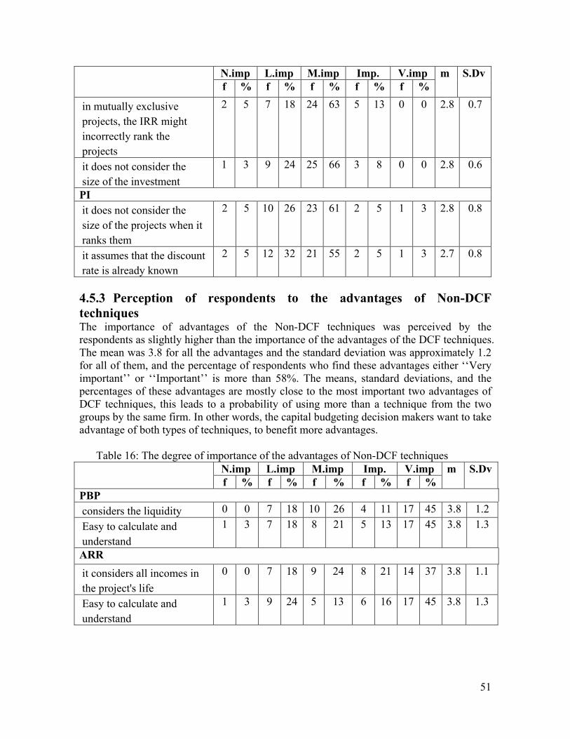
51

N.imp L.imp M.imp Imp. V.imp f % f % f % f % f %

m S.Dv

in mutually exclusive

projects, the IRR might

incorrectly rank the

projects

2 5 7 18 24 63 5 13 0 0 2.8 0.7

it does not consider the

size of the investment

1 3 9 24 25 66 3 8 0 0 2.8 0.6

PI

it does not consider the

size of the projects when it

ranks them

2 5 10 26 23 61 2 5 1 3 2.8 0.8

it assumes that the discount

rate is already known

2 5 12 32 21 55 2 5 1 3 2.7 0.8

4.5.3 Perception of respondents to the advantages of Non-DCF techniques The importance of advantages of the Non-DCF techniques was perceived by the respondents as slightly higher than the importance of the advantages of the DCF techniques. The mean was 3.8 for all the advantages and the standard deviation was approximately 1.2 for all of them, and the percentage of respondents who find these advantages either ‘‘Very important’’ or ‘‘Important’’ is more than 58%. The means, standard deviations, and the percentages of these advantages are mostly close to the most important two advantages of DCF techniques, this leads to a probability of using more than a technique from the two groups by the same firm. In other words, the capital budgeting decision makers want to take advantage of both types of techniques, to benefit more advantages.

Table 16: The degree of importance of the advantages of Non-DCF techniques N.imp L.imp M.imp Imp. V.imp f % f % f % f % f %

m S.Dv

PBP

considers the liquidity 0 0 7 18 10 26 4 11 17 45 3.8 1.2

Easy to calculate and

understand

1 3 7 18 8 21 5 13 17 45 3.8 1.3

ARR

it considers all incomes in

the project's life

0 0 7 18 9 24 8 21 14 37 3.8 1.1

Easy to calculate and

understand

1 3 9 24 5 13 6 16 17 45 3.8 1.3

52

4.5.4 Perception of respondents to the disadvantages of Non-DCF techniques The importance of disadvantages of the Non-DCF techniques seems to be higher than the importance of disadvantages of the DCF techniques. The average mean of these advantages was obviously higher and the trend of the answers of the respondents were more concentrated on ‘‘Very important’’ and ‘‘Important’’, rather than ‘‘Low importance’’ and ‘‘Moderate importance’’ as in the disadvantages of the DCF techniques. The mean for the importance of these disadvantages was about 3.1 and the standard deviation was about 1.2.

Table 17: The degree of importance of the disadvantages of Non-DCF techniques

N.imp L.imp M.imp Imp. V.imp f % f % f % f % f %

m S.Dv

PBP

it does not consider the

time value of money

1 3 10 26 12 32 5 13 10 26 3.3 1.2

it does not reflect the

profitability of the project

1 3 10 26 12 32 5 13 10 26 3.2 1.2

it does not consider the

cash flow after the PBP

2 5 10 26 13 34 6 16 7 18 3.2 1.2

ARR

it does not consider the

time value of money

1 3 13 34 10 26 4 11 10 26 3.2 1.3

it ignores the cash flows 1 3 13 34 11 29 5 13 8 21 3.2 1.2

it ignores the lives of the

projects

2 5 13 34 14 37 1 3 8 21 3.0 1.2

Based on the previous analysis of the importance of the advantages and disadvantages, we can conclude that the respondents perceive the advantages of the techniques more important than the disadvantages. The respondent perceived the advantages of the DCF techniques and the Non-DCF as the most important ones, while they perceived moderate importance for the disadvantages of the DCF techniques, and they perceived the disadvantages of the Non-DCF techniques as important.

4.6 The relationship between the perception of the respondents to the

advantages and disadvantages of the techniques and their use As done in the previous analyses in this study, the analysis of this part is run on the replacement decisions and then is addressed to all other type of investment decisions. The relationship between the variables of this part is measured by Chi-test square for independence; we were recommended to use it because that our sample is very small (Pallant, 2007, p. 210), Pearson correlation, and Cramer’s V. As the second question is about finding the reasons for using some capital budgeting techniques rather than other, this part is an attempt to explore if the perception of the respondents to the advantages and disadvantages of the techniques are the reasons for degree of the use.

53

The relationship between the advantages and disadvantages of NPV and

its use For the relationship between the degree of using NPV and its advantages, all conducted tests produced coefficients that have positive sign and strong relationship; no less than 0.50 and these results are statistically significant at 0.05 level. This means that the perception of respondents to the advantages of the NPV positively and strongly affect its use. While for the relationship between the degree of using NPV and its disadvantages, the results showed a very small relationship; less than 0.10 and these result are statistically insignificant at 0.05 level. We can say that the perception of the respondents to the disadvantages of the NPV does not affect its use. This finding agrees with the previous finding about the importance of the NPV techniques’ advantages, agrees with the finding that NPV is the second most used technique, and agrees with the finding that advantages of NPV techniques were perceived to be important by the respondents. Also the finding agrees with perception of the respondents to the disadvantages of the NPV, where the respondents perceive them as less than moderately important.

The relationship between the advantages and disadvantages of IRR and

its use For the relationship between the degree of using IRR and its advantages, all conducted tests produced statistically insignificant results at 0.05 level, this means that the perception of respondents to the advantages of the IRR does not affect its use. This part agrees with the previous findings; the IRR is the least used techniques, and its advantages are perceived to be least important ones compared to advantages of the NPV and the PI. While for the relationship between the degree of using IRR and its disadvantages; except for the disability of IRR to handle non conventional cash flow, the results are statistically insignificant at 0.05 level. We can say that the perception of the respondents to the disadvantages of the IRR affect its use.

The relationship between the advantages and disadvantages of PI and its

use For the relationship between the degree of using PI and its advantages, all conducted tests produced coefficients that have positive sign and medium strength relationship for the advantage that PI considers all cash flows during the life of the project. While the advantage that PI consider the time value of money, and the advantage of ability to rank projects are only statistically significant using Pearson correlation. This correlation is positive and has a medium strength. This finding is consistent with the finding about the degree of using PI and the finding about the perception of PI’s advantages. For the disadvantages, all statistical tests showed insignificant results.

The relationship between the advantages and disadvantages of PBP and

its use For the relationship between the degree of using PBP and its advantages, all conducted tests produced coefficients that have positive sign and strong or medium strength relationship. These results are statistically significant at 0.05 level; this means that the perception of respondents to the advantages of the PBP positively and strongly affect its use. This finding

54

agrees with the finding about the use of PBP as the most used technique, and the finding about the respondents’ perception of the advantages of the PBP as important ones. While for the relationship between the degree of using PBP and its disadvantages, the results are statistically insignificant at 0.05 level. We can say that the perception of the respondents to the disadvantages of the NPV does not affect its use.

The relationship between the advantages and disadvantages of ARR and

its use For the relationship between the degree of using ARR, and its advantages and disadvantages, all conducted tests produced insignificant results. These results make sense since the ARR is used less than low use by 73% of the respondents.

Comprehensive statement about the relationship between the advantages

and disadvantages of the techniques and their use Advantages of PBP, NPV, and PI have a positive effect on the degree of using them, while the disadvantages of all capital budgeting techniques do not show any significant effect on the degree of using the techniques. The researchers reject the fifth null hypothesis; ‘‘the perception of the respondents to the advantages and disadvantages of capital budgeting techniques is not the reason for the degree of using capital budgeting techniques.’’, and instead, accept the alternative hypothesis.

4.7 Relationship between capital budgeting sophistication and firms’

performance Brief reminder

Recalling the used model that measures if any relationship between the degree of sophistication and performance of the firm exists, which is as follows: OIROA j= b0+ b1ATj+ b2DCBSj

Where: OIROA j= operating rate of return for firm j ATj= Size of firm j DCBSj= Degree of capital budgeting sophistication for firm j In this study, only two independent variables are used to explain the dependent variable. Some other variables are used by other researchers in their studies, but those variables do not fit this study for different reasons. For example, the variables used by Farragher et al (2001, p. 303), either need a long time series to gather their data, or they are made particularly to serve a specific objective of their study, like the adjustment for the industry. This study is restricted by a time table and it is applied on one industry. The demographical characteristics of the respondents in this study could have been included in the regression analysis, but the respondents were so much alike in their demographical characteristics. This might be attributed to the size of the sample, which was a very small one. This alikeness in the demographical characteristics might not give a reasonable result in explaining the dependent variable, so, the researchers of this study

55

chose the variables that are consistent with their beliefs in accordance with their expectations and limitations. Operating performance

OIROA is the operating rate of return of a firm measured by dividing the cash flow from the operating activities in the cash flow statement by the total assets of the firm. The data has been gathered from the 2009 financial statements of the firms as submitted to Jordan securities commission JSC. The JSC is supposed to disclose all of the firms’ financial statements, some of the firms’ financial statements could not be found at the JSC web page and the researchers had access to only 30 firms of them. In this study OIROA represents the dependent variable in the multiple regression model. The operating rate of return for the firms under current analysis ranges from -12% to 38% and their average mean is 8%. Size of firm

AT is the size of firm represented by the total assets of a firm. In this study AT represents the independent variable in the multiple regression model. The data has been gathered from the 2009 financial statements of the firms as submitted to JSC. Degree of sophistication

The degree of sophistication for the firms has been determined after receiving back the questionnaire. As explained before, the firm’s degree of sophistication is based on the use of specified practices; these are, using any of the DCF techniques, using WACC to determine the discount rate, and using any of the analytical techniques to analyze for risk. The weight for each activity was based on the respondents’ answers. After analyzing the answers and the degree of importance or use, the activities’ weights were as follows: The use of DCF technique gives the firm 35% degree of sophistication The use of WACC gives the firm 35% degree of sophistication The use of analytical techniques when analyzing for risk gives the firm 30% degree of sophistication. Figure 4: firm’s degree of sophistication

56

Regression analysis

In statistics, R square value states (in percentage) the variance in the dependent variable which is explained by the model, while the complementary percentage explains the random factors affecting the model, like missing variables. The researchers chose the adjusted R square since it takes into account any missing or extra variables in the model (Najeeb, & Alrefay, 2006, p. 351). To evaluate the model, the researchers relied on the adjusted R square; which showed that the model explains -4% of the variance in the operating performance, and this is a quite small per cent to be explained by a model. In addition, this result is statistically insignificant according to ANOVA test. Finally, we can say that the model is not fit enough to explain the dependent variable, either because of little size of the sample, or because of missing independent variables in the model. For future studies, we recommend more variables and larger sample size. Both the degree of sophistication and the firm size have a small contribution in predicting operating performance, -.09 for degree of sophistication and 0.17 for firm size. Both results are statistically insignificant when checking the t-test significance level. To write the equation of the model as extracted from the coefficient analysis, we take the Un-standardized coefficient (Pallant, 2007, p. 159): OIROA j= 0.078+ 1.219ATj - 0.023 DCBSj

57

The coefficients of the variables in this equation give the following data: The t value of each coefficient is: B0=2.82, B1=0.862, B2= -0.425. The significance of each value is: 0.009, 0.396, and 0.674 respectively in the same previous order. The Pearson correlation test indicates a small relationship between the operating performance on one hand and the degree of sophistication and the firm size on the other hand. This result was statistically insignificant at 0.05 level. Both independent variables have a medium positive relationship and this result is statistically significant at level 0.05. We can conclude that according to the multiple regression analysis, the researchers found that there is no any indication for a relationship between the degree of sophistication and the operating performance of the firms. Moreover, there was no relationship between the firm’s size and its operating performance. Based on this finding, the researchers accept the sixth null hypothesis ‘‘the firms with higher capital budgeting sophistication do not perform better than firms with less capital budgeting sophistication’’. The results were similar to those previous studies conducted by Ramadan (1991) but were different from those of Farragher et al (2001) who found a negative relationship between the performance and the use of sophisticated capital budgeting. Jiang et al (2006) found a positive relationship between the performance of the firms measured by the earning and the capital expenditures.

58

Chapter.5 Conclusion and credibility criteria

5.1 Conclusion This study is an empirical evidence to explore the use of capital budgeting techniques and its related practices by Jordanian listed services firms. After analyzing 38 firms, the researchers found that PBP is the most used capital budgeting technique by Jordanian services listed firms, followed by NPV, PI, ARR, and IRR. The results showed that the Jordanian services listed firms use DCF techniques, as well as Non-DCF, when assessing capital investment projects. The researchers studied some practices that relate to the capital budgeting process; these are, cost of capital estimation practices, risk analysis practices, and cash flow forecasting practices. They found that these practices are not widely used by capital budgeting decision makers of the Jordanian services listed firms since subjective judgment is more widely applied. The researchers studied some factors that might be leading the capital budgeting decision maker to use the above mentioned techniques in that order. The type of capital investment decision was thought be one of the reasons that justify the degree of using capital budgeting techniques. After analyzing the answers of the respondents, it was clear that the type of capital investment decision has no effect on the degree of using capital budgeting technique. Most of the respondents in the sample were older than 35 years, academically qualified, professionally unqualified, and experienced. These demographical characteristics of the sample had been studied by the researchers to see if any of them has an influence on the selection of the capital budgeting techniques or its degree of use. Academic qualification has a significant influence on the use of capital budgeting techniques; the higher the academic qualification enjoyed by the capital budgeting decision maker, the more he applies DCF techniques. The perception of the respondents to the advantages and disadvantages of each technique is the most important factor of the choice of capital budgeting technique and its degree of use. The advantages of Non-DCF techniques are more important than the advantages of DCF techniques which explain the high use of the PBP. The advantages of PBP and advantages of NPV explain their degree of use since they are the most used techniques by the respondents. After measuring the relationship between the degree of capital budgeting sophistication and the operating performance, the researcher found no relationship between the two variables. So, our results do not support the theoretical assumption that firms which use more sophisticated capital budgeting techniques perform better than firms with a less degree of capital budgeting sophistication. In conclusion, the researchers found that capital budgeting decision makers of Jordanian listed firms use both DCF techniques and Non-DCF techniques. The degree of using the techniques ordered from the most used one to the least used one is; PBP, NPV, PI, ARR, and IRR. Comparing this finding to the findings of studies addressing Jordanian firms, this finding is different from Ramadan’s (1991) who found that the most used techniques are NPV, PI, and PBP, and it is different from Khamees et al’s (2010) who found that the most

59

used techniques are PI, PBP, and IRR. The researchers’ finding is consistent with some other studies conducted on different countries like Mao (1970), and Block (1997), where the most used technique was the PBP, but this finding is inconsistent with some other studies, like Jog & Srivastava (1995), Kester et al. (1999), and Ryan & Ryan (2002); they all found a preference to the DCF techniques. The capital budgeting decision makers’ perception to the advantages of some technique explains the extent of their use. The advantages of PBP, NPV, and PI positively affect the degree of using these techniques. Some demographical characteristics affect the degree of using the techniques, for example, as age and academic qualification increase, the degree of using IRR decreases and the degree of using NPV and PI increases respectively. There was no relationship between the degree of capital budgeting sophistication and the firms’ performance. This specific result is similar to those previous studies conducted by Ramadan (1991); where he found no evidence on this claimed relationship, but this finding is different from those of Farragher et al (2001) who found a negative relationship between the performance and the use of sophisticated capital budgeting. The researchers’ finding is different from Jiang et al.’s (2006) who found a positive relationship between the performance of the firms measured by the earning and the capital expenditures. At the Jordanian level, the researchers recommend a further study on Jordanian firms, through which a comparison can be made based on industry sectors; where more firms are included in the sample to give more generalization and to benefit more sectors. Regarding the relationship between the performance and the degree of capital budgeting sophistication, the researchers recommend further studies to include more firms; this will increase the fitness of the model that measures the possible relationship. At the regional level, the researchers recommend more research in the field of the capital budgeting since very rare researches had been conducted. At the international level, the researchers believe that most of the previously conducted studies are much more descriptive than analytical, so the researchers recommend further studies that try to link capital budgeting to any possible issues; like the viability of the firms, firms’ competitiveness, and productivity. Finally, this study is an attempt to give empirical evidence on the capital budgeting techniques in Jordan, and it helps to give more insight into the theory and practice of this topic.

5.2 Generalization The generalization of any study’s results can be made only to the population from which the sample was taken, even if the sample was drawn through a probability sampling (Bryman, & Bell, 2007, p. 203). Since the population of this study was the Jordanian listed services firms, the results are only addressed to this specific population. The sample of this study was the whole population, and the percentage of the usable replies was 60%. So, we can fairly generalize the results of this study to the Jordanian listed

60

services firms. But for other Jordanian firms, we think that the findings of this study can be fruitful and can give them a better general insight into the capital budgeting in Jordan. The findings of this study can also be beneficial to some countries in the region given that they have some similar economical conditions and investment climate.

5.3 Validity and reliability Validity test is applied to check if the research tool measures what it is supposed to measure, this includes two types of validity tests; face validity and contents validity. After forming the preliminary structure and contents of the questionnaire it was presented to the supervisor of the thesis. He recommended a list of text books to read, and after reviewing some parts of these books, a modified version of the questionnaire was presented to the supervisor again, some final modifications were suggested from his side, and a final questionnaire was developed (Sekaran, 2003, p. 206).

Reliability tests indicate the degree, to which the scale is free from random errors (Pallant, 2007, p. 6), this means testing the possibility of having the same results if the study is conducted on different occasions or by different observers (Saunders et al., 2003, p. 101). Two types of tests are used to measure the reliability; the test-retest reliability and internal consistency. The former is conducted by distributing the questionnaire on the same people on two different occasions. High test-retest correlations indicate a stronger reliable scale. While the latter measures the degree to which the items of a scale are measuring the same underlying attribute. The most used test to measure the internal consistency is cronbach’s alpha coefficient (Pallant, 2007, p. 6). In this study and due to the time and communications limits, the only reliability test used is the internal consistency test; that is, Cronbach’s alpha coefficient through SPSS. Statistically, the value of this coefficient ranges from 0 to 1 given that higher value indicates more reliability. The minimum recommended level is 0.7 (Pallant, 2007, p. 6). According to the structure of the questionnaire, the questions it includes, and the variables it studies, the researchers have conducted the reliability test on three aspects by dividing the questionnaire into three parts. The first part represents the use of capital budgeting techniques in different decisions situations; the value of cronbach’s alpha coefficient for this part is 0.853. The second part represents the advantages and disadvantages of capital budgeting techniques; the value of cronbach’s alpha coefficient for this part is 0.919. The third part represents the practices applied with capital budgeting techniques; risk analysis practices, cost of capital estimation practices, and cash flow forecasting practices, the value of cronbach’s alpha coefficient for this part is 0.921. All values are relatively high and indicate a high reliability.

5.4 Implications The findings of this research address important contributions to theory and practice aspects of capital budgeting field. They can be seen as follows: In practice, the degree of using capital budgeting techniques and their related practices by Jordanian listed services firms and the reasons behind it might help the practitioners to identify the environmental aspects that affect their choices. These environmental aspects

61

include the perception of the practitioners themselves, the firm, the industry, and the limitations on those aspects. So, the findings of this research could be seen as an available effort to every practitioner of capital budgeting; at least to give him a better understanding about the subject. In theory, this research represents a fruitful comprehensive summary of the most important concepts of capital budgeting; where the researchers made sure to choose the books and articles which provide reliable information and findings. Students of finance, accounting, and other field of business can benefit from this research when reading about the subject or trying to relate theory to practice.

62

References

Books • Arnold, G. (2008). Corporate financial management, 4th edition, London, Prentice

Hall. • Bierman, H.Jr., & Smidt, S. (1966). The capital budgeting decision: economic

analysis and financing of investment projects, 2nd edition, New York, Macmillan Company.

• Blocher, E.J., Stout, D.E., Cokins, G., & Chen, K.H. (2008). Cost management: A strategic emphasis, 4th international edition, New York, Mc Graw Hill.

• Brealey, R.A., Myers, S.C., & Allen, F. (2006). Corporate finance, 8th international edition, New York, Mc Graw Hill.

• Bryman, A., & Bell, E. (2007). Business research methods, 2nd edition, New York, Oxford University press.

• Cherry, R.T. (1970). Introduction to business finance, California, Wadsworth publishing company.

• Cohen, L., Manion, L., & Morrison, K. (2000). Research methods in education, 5th edition, New York, Routledge Falmer.

• Cooper, D.R., Schindler, P.S. (2003). Business research methods, • Creswell, J.W. (2003). Research design, 2nd edition, California, Sage Publications • Dayananda, D., Irons, R., Harrison, S., Herbohn, J., & Rowland, P. (2002). Capital

budgeting: financial appraisal of investment projects, 1st edition, Cambridge, Cambridge University press.

• Drury, C. (2005). Management accounting for business, 4th edition, London, Thomson.

• Drury, C. (1996). Management and cost accounting, 3rd edition, London, Thomson. • Eakins, S.G. (1999). Finance: investments, institutions, & management, 1st edition,

New York, Addison-Wesley. • Gitman, L.G. (1987). Basic managerial finance, 1st edition, New York, Harper &

Row publisher • Gratton, C., Jones, I. (2004). Research methods for sport studies, 1st edition, New

York, Routledge • Helve, H., Giani, F., Honkasalo, V., Kauppinen, T.M., Kuusisito, A., Louhivuori, L.,

& et al. (2005). Mixed methods in youth research, 1st edition, Helsinki, Finnish youth research

• Hilton, R. (2005). Managerial Accounting, 6th edition, New York, Mc Graw Hill. • Hirsch, M.L. (1994). Advanced management accounting, 2nd edition, Ohio, South-

western publishing Co. • Hirschey, M. (2003). Managerial economics, 10th edition, Ohio, Thomson-south

western. • Johns, N., & Lee-Ross, D. (1998). Research method in service industry

management, 1st edition, New York, Cassell • Levy, H., Sarnat, M. (1986). Capital investment and financial decisions, 3rd edition,

London, Prentice Hall international.

63

• Pallant, J. (2007). SPSS: Survival manual, 1st edition, New York, Mc Graw Hill • Penman, S. (2010). Financial statement analysis and security valuation, 4th edition,

New York, Mc Graw Hill. • Pike, R., Neale, B. (2003). Corporate finance and investment, 4th edition, England,

Essex, Prentice hall • Ryan, B., Scapens, R., Theobald, M. (1992). Research method and methodology in

finance and accounting, 1st edition, California, Academic Press. • Saunders, M., Lewis, P., Thornhill, A. (2003). Research methods for business

students, 3rd edition, England, Essex, Prentice hall • Schmidgall, R.S. (1995). Hospitality industry managerial accounting, 3rd edition,

Michigan, Educational institute • Sekaran, U. (2003). Research methods for business, 4th edition, New York, John

Wiley & sons, Inc • Williamson, D. (1996). Cost and management accounting, Hertfordshire, Prentice

halleurope.

Articles • Agmon, T. (1991). Capital Budgeting and the Utilization of Full Information:

Performance Evaluation and the Exercise of Real Options, Managerial finance, 17 (2-3), 42-50.

• Alkaraan, F., & Northcott, D. (2007). Strategic investment decision making: the influence of pre-decision control mechanisms, Qualitative Research in Accounting & Management, 4 (2), 133-150.

• Arnold, G.C., & Hatzopoulos, P.D. (2000). The theory practice gap in capital budgeting: evidence from the U.K, Journal of business finance and accounting, 27 (5&6), 603-626.

• Bennouna, B., Meredith, G., & Marchant, T. (2010). Improved capital budgeting decision making: evidence from Canada, Management Decision, 48 (2), 225-247.

• Block, S. (1997). Capital budgeting techniques used by small business firms in 1990s, The engineering economist, 42 (4), 289-302.

• Brounen, D., Jong, A., & Koedijk, K. (2004). Corporate Finance in Europe: Confronting Theory with Practice, Financial Management, 33 (4), 71-101.

• Chatrath, A., & Seiler, M.J. (1997). Capital Budgeting and the Stochastic Cost of Capital, Managerial finance, 23 (9), 16-23.

• Cooper, W.D., Morgan, R.G., Redman, A., & Smith, M. (2001). Capital budgeting models: Theory VS. Practice, Business forum, 26 (1&2), 15-19.

• Danielson, M.G, & Scott, J.A. (2006). The capital Budgeting Decisions of Small Businesses, Journal of applied finance, 16 (2), 45-56.

• El-ebaishe, M., Karbhari, Y., & Naser, K. (2003). Empirical evidence on the use of management accounting techniques in a sample of Saudi manufacturing companies, IJCM, 3 (2), 74-101.

• Farragher, E.J., Kleiman, R.T., & Sahu, A.P. (2001). The association between the use of sophisticated capital budgeting practices and corporate performance, The engineering economist, 46 (4), 300-311.

64

• Graham, G., Harvey, C. (2002). How do CFOs make capital budgeting and capital structure decisions, Journal of applied corporate finance, 15 (1), 8-24.

• Haka, S.F., Gordon, L.A., & Pinches, G.E. (1985). Sophisticated Capital Budgeting Selection Technique And Firm Performance, The Accounting Review, LX (4), 651-668.

• Hatfield, P., Hill, D., Horvath, P. (1998). Industrial buying and divergence of capital budgeting theory and practice: an exploration, The journal of applied business research, 15 (1), 37-46.

• Hermes, N., Smid, P., & Yao, L. (2007). Capital Budgeting Practices: A Comparative Study of the Netherlands and China, International business review, 16 (5), 630-654.

• Hull, J.C. (1986). Risk in capital investment proposals: three viewpoints, Managerial finance, 12 (3), 12-15.

• Jiang, C.H., Chen, H.L., & Huang, Y.S. (2006). Capital expenditures and corporate earnings: Evidence from the Taiwan Stock Exchange, Managerial Finance, 32 (11), 853-861.

• Jog, V.M., & Srivastava, A.K. (1995). Capital budgeting practices in corporate canada, Financial Practice and Education, 5 (2), 37-43.

• Kester, G.W., Chang, R.P., Echanis, E.S., Haikal, S., Isa, M.Md., Skully, M.T. & et al. (1999). Capital budgeting practices in the Asia-pacific region: Australia, Hong Kong, Indonesia, Malaysia, Philippines, And Singapore. Financial practice and education, 9 (1), 25-33.

• Khamees, B.A., Al-Fayoumi, N., & Al-Thuneibat, A. (2010). Capital budgeting practices in the Jordanian industrial corporations, International Journal of Commerce and Management, 20 (1), 49-63.

• Lazaridis, I.T. (2004). Capital Budgeting Practices: A survey in the firms in Cyprus, Journal of small business management, 42 (4), 427-433.

• Mao, J.C. T. (1970). Survey of capital budgeting: theory and practice, The journal of finance, 25 (2), 349-360.

• Pike, R. (1996). A longitudinal survey on capital budgeting practices, Journal of business finance & accounting, 23 (1), 79-92.

• Pike, R. (1981). Capital budgeting and corporate performance, Management research news,4 (1).

• Ryan, P.A., & Ryan, G.P. (2002). Capital budgeting practices of the fortune 1000: how have things changed?, Journal of Business and Management, 8 (4), 355-364.

• Schall, L.D., Sundem, G.L., & Geusbeek, W.R. (1978). Notes survey and analysis of capital budgeting methods, The journal of finance, 33 (1), 281-287.

• Smith, D.J. (1994). Incorporating risk into capital budgeting decisions using simulation, Management decision, 32 (9), 20-26.

• Truong, G., Partington, G., & Peat, M. (2008). Cost-of-capital estimation and capital-budgeting practice in Australia, Australian journal of management, 33 (1), 95-121.

• Verma, S.,Gupta, S., & Batra, R. (2009). A Survey of capital budgeting practices in Corporate India, The journal of business perspective, 13 (3), 1-17.

65

• White, J.B., Morgan, P.M., & Munilla, L.S. (1997). An exploratory study into the adoption of capital budgeting techniques by agricultural co-operatives, British food journal, 99 (4), 128–132.

Arabic sources • Ramadan, S. (1991). Capital budgeting techniques and firm performance: Jordanian

industrial corporations, Majalat jameat almalik saud: alolom aledareiah (Journal of university of king Saud: business sciences), 3 (1), 187-212.

• Najeeb, H., & Alrefay, G. (2006). Analyzing data using computer: comprehensive use of SPSS, 1st edition, Amman, Alahliah

Electronic sources • Country profile – Jordan (2006), http://memory.loc.gov/frd/cs/profiles/jordan.pdf. • www.ase.com.jo • www.cbj.gov.jo • Foreign investment climate (2010), Jordan country review, p58-61.

www.web.ebscohost.com • http://www.jsc.gov.jo/

66

Appendix 1: The questionnaire

Questionnaire

Title of the study: ‘‘Capital budgeting technique and firm performance Case study: Jordanian listed services firms’’ Dear capital budgeting decision maker The researchers are conducting a study about the capital budgeting practices in Jordan. The study targets the listed services firms, and to achieve its objectives, this questionnaire has been developed. Please read and answer the questions carefully, knowing that all provided information will be used only for scientific research, and will be treated confidentially.

Thanks for your cooperation Researchers: Abdallah Alzoubi: Abal0012@student.umu.se Yasir Alazawi: Yaal0002@student.umu.se Supervisor: Åke Gabrielsson: Ake.gabrielsson@usbe.umu.se Business school Umea University Umea, Sweden

67

Part one: demographical information

(Please answer by typing (x) in the given space). Age:

( ) 24 years or less ( ) 25 – 34 years ( ) 35 – 44 years ( ) 45 years or more

Academic qualification:

( ) High school or below ( ) Community college ( ) Bachelor degree ( ) Master degree ( ) P.HD degree

Professional qualification:

( ) None ( ) Certified Managerial Accountant ( ) Certified Financial Manager ( ) Jordanian Certified Public Accountant ( ) Certified Public Accountant ( ) Others …………

Experience:

( ) 2 years or less ( ) 3 -12 years ( ) 13 – 22 years ( ) 23 years or more

Part two: the use of capital budgeting techniques 1- To what extent the following techniques are used to take the following decisions:

Please answer by typing (x) in the box that fits your degree of use.

Replacement Decisions Seldom Low use Moderate use High use Always

Net Present Value NPV

Internal Rate of Return IRR

Profitability Index PI

Pay Back Period PBP

Accounting Rate of Return ARR

Other used techniques, if any: ……………………

Expansion Decisions Seldom Low use Moderate use High use Always

Net Present Value NPV

Internal Rate of Return IRR

Profitability Index PI

Pay Back Period PBP

Accounting Rate of Return ARR

Other used techniques, if any: ……………………

68

Lease or Buy Decisions Seldom Low use Moderate use High use Always

Net Present Value NPV

Internal Rate of Return IRR

Profitability Index PI

Pay Back Period PBP

Accounting Rate of Return ARR

Other used techniques, if any: ……………………

Independent Projects Decisions (where the selection of the a project does not affect the selection of other projects)

Seldom Low use Moderate use High use Always

Net Present Value NPV

Internal Rate of Return IRR

Profitability Index PI

Pay Back Period PBP

Accounting Rate of Return ARR

Other used techniques, if any: ……………………

Mutually Exclusive Projects Decisions (where the acceptance of a project eliminates all other projects, and contingent projects)

Seldom Low use Moderate use High use Always

Net Present Value NPV

Internal Rate of Return IRR

Profitability Index PI

Pay Back Period PBP

Accounting Rate of Return ARR

Other used techniques, if any: ……………………

Contingent Projects Decisions (where the acceptance or rejection of a project is dependent on the acceptance or rejection of one or more other projects)

Seldom Low use Moderate

use

High use Always

Net Present Value NPV

Internal Rate of Return IRR

Profitability Index PI

Pay Back Period PBP

Accounting Rate of Return ARR

Other used techniques, if any: ……………………

69

Part three: the degree of importance of the advantages and disadvantages of

capital budgeting techniques:

1- The degree of importance of the advantages of the discounted cash flow techniques

Not

important

Low

importance

Moderate

importance

important Very

important

Net Present Value NPV It considers the time value of money

It considers all cash flows during the life of the project

It assumes that the cash inflows are reinvested

It handles non conventional cash flows

It is consistent with the concept of maximizing the shareholders’ wealth

Internal Rate of Return IRR

It considers the time value of money It considers all cash flows during the life of the project

It gives a percentage measure It is consistent with the concept of increasing the firm’s value

Profitability Index PI It considers the time value of money It considers all cash flows during the life of the project

It gives a relative measure to rank projects according to their profitability

2- The degree of importance of the disadvantages of the discounted cash flow techniques

Not

important

Low

importance

Moderate

importance

important Very

important

Net Present Value NPV It does not give a percentage measure, only absolute amount. Which does not give the best project among different sizes mutually exclusive alternatives

It assumes that the discounting rate is already known

It does not consider the size of the investment

Internal Rate of Return IRR It can not handle non conventional

70

Not

important

Low

importance

Moderate

importance

important Very

important

cash flows Financing type decision may misinterpret the calculation result.

In mutually exclusive project, the IRR might incorrectly rank the projects

It does not consider the size of the investment

Profitability Index PI

It does not consider the size of the projects when it ranks them

It assumes that the discounting rate is already known

3- The degree of importance of the advantages of the Non- discounted cash flow techniques

Not

important

Low

importance

Moderate

importance

important Very

important

Pay Back Period PBP

The length of the PBP gives an indication about the risk factor (considers the liquidity)

Easy to calculate and to understand

Accounting Rate of Return ARR

It considers all incomes in the project’s life

Easy to calculate and understand

4- The degree of importance of the disadvantages of the Non- discounted cash flow techniques

Not

important

Low

importance

Moderate

importance

important Very

important

Pay Back Period PBP

It does not consider the time value of money

It does not reflect the profitability of the project

It does not consider the cash flows after the pay back period

Accounting Rate of Return ARR It ignores the time value of money It ignores the cash inflows (considers the accounting income)

It ignores the lives of the projects

71

Part four: practices related to capital budgeting 1- If you use any of the discounted cash flow techniques (Net Present Value, Internal Rate of Return, and

Profitability Index), to which extent the followings are used to determine the discounting rate: Seldom Low use Moderate

use

High use Always

Weighted average cost of capital

Cost of borrowing at banks

Cost of borrowing through bonds

Cost of common stocks

Cost of equity

Past experience

Others, if any: …………………… 2- If you analyze for risk, to which extent the following practices are used:

Seldom Low use Moderate

use

High use Always

Probability distribution

Simulation analysis

Decision tree

Sensitivity analysis

Risk adjusted cash flows

Risk adjusted pay back period

Risk adjusted discount rate

Subjective judgment

Others, if any: …………………. 3- When forecasting the cash flows of a project, to which extent the following practices are used:

Seldom Low use Moderate

use

High use Always

Simple regression analysis

Multiple regression analysis

Time-trend projections

Moving averages

Delphi method

Nominal group technique

Jury of executive opinion

Scenario projection

Others, if any: …………………..

72

Appendix 2: Demographical characteristics of the sample

Statistics

Age

Academic

qualification

Professional

qualification Experience

Valid 38 38 38 38 N

Missing 0 0 0 0

Mean 2,8421 3,1316 1,3421 2,9211

Std. Deviation ,91611 ,66459 ,93798 ,85049

Age

Frequency Percent Valid Percent

Cumulative

Percent

1,00 24 years or less 2 5,3 5,3 5,3

2,00 25-34 years 13 34,2 34,2 39,5

3,00 35-44 years 12 31,6 31,6 71,1

4,00 45 years or more 11 28,9 28,9 100,0

Valid

Total 38 100,0 100,0

Academic qualification

Frequency Percent Valid Percent

Cumulative

Percent

2,00 Community college 6 15,8 15,8 15,8

3,00 Bachelor degree 21 55,3 55,3 71,1

4,00 Master degree 11 28,9 28,9 100,0

Valid

Total 38 100,0 100,0

Professional qualification

Frequency Percent Valid Percent

Cumulative

Percent

1,00 None 33 86,8 86,8 86,8

2,00 Certified Managerial

Accountant

1 2,6 2,6 89,5

4,00 Jordanian Certified

Public Accountant

4 10,5 10,5 100,0

Valid

Total 38 100,0 100,0

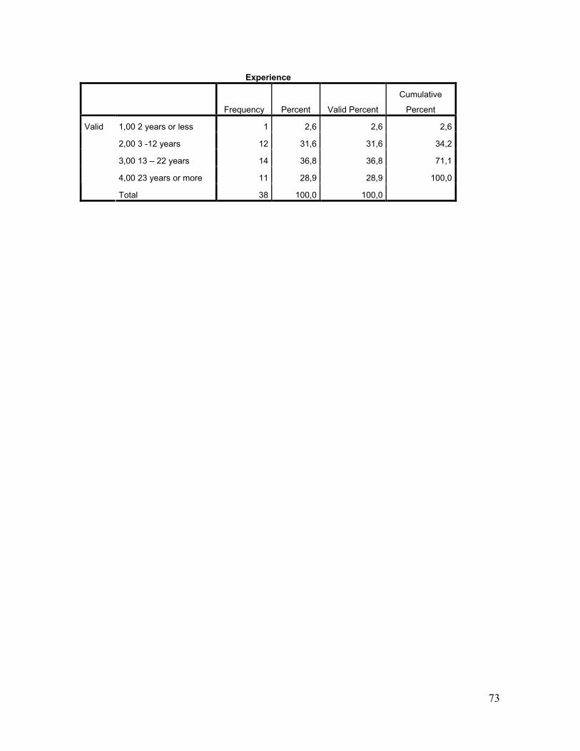
73

Experience

Frequency Percent Valid Percent

Cumulative

Percent

1,00 2 years or less 1 2,6 2,6 2,6

2,00 3 -12 years 12 31,6 31,6 34,2

3,00 13 – 22 years 14 36,8 36,8 71,1

4,00 23 years or more 11 28,9 28,9 100,0

Valid

Total 38 100,0 100,0

74

Appendix 3: Degree of using capital budgeting techniques

Replacement Decisions NPV

Frequency Percent Valid Percent

Cumulative

Percent

1,00 Seldom 14 36,8 36,8 36,8

2,00 Low use 9 23,7 23,7 60,5

3,00 Moderate use 2 5,3 5,3 65,8

4,00 High use 2 5,3 5,3 71,1

5,00 Always 11 28,9 28,9 100,0

Valid

Total 38 100,0 100,0

Replacement Decisions IRR

Frequency Percent Valid Percent

Cumulative

Percent

1,00 Seldom 21 55,3 55,3 55,3

2,00 Low use 14 36,8 36,8 92,1

3,00 Moderate use 2 5,3 5,3 97,4

5,00 Always 1 2,6 2,6 100,0

Valid

Total 38 100,0 100,0

Replacement Decision PI

Frequency Percent Valid Percent

Cumulative

Percent

1,00 Seldom 17 44,7 44,7 44,7

2,00 Low use 9 23,7 23,7 68,4

3,00 Moderate use 2 5,3 5,3 73,7

4,00 High use 2 5,3 5,3 78,9

5,00 Always 8 21,1 21,1 100,0

Valid

Total 38 100,0 100,0

75

Replacement Decision PBP

Frequency Percent Valid Percent

Cumulative

Percent

1,00 Seldom 11 28,9 28,9 28,9

2,00 Low use 2 5,3 5,3 34,2

3,00 Moderate use 3 7,9 7,9 42,1

4,00 High use 10 26,3 26,3 68,4

5,00 Always 12 31,6 31,6 100,0

Valid

Total 38 100,0 100,0

Replacement Decision ARR

Frequency Percent Valid Percent

Cumulative

Percent

1,00 Seldom 21 55,3 55,3 55,3

2,00 Low use 7 18,4 18,4 73,7

3,00 Moderate use 1 2,6 2,6 76,3

4,00 High use 2 5,3 5,3 81,6

5,00 Always 7 18,4 18,4 100,0

Valid

Total 38 100,0 100,0

Expansion Decisions NPV

Frequency Percent Valid Percent

Cumulative

Percent

1,00 Seldom 14 36,8 36,8 36,8

2,00 Low use 9 23,7 23,7 60,5

3,00 Moderate use 2 5,3 5,3 65,8

4,00 High use 1 2,6 2,6 68,4

5,00 Always 12 31,6 31,6 100,0

Valid

Total 38 100,0 100,0

76

Expansion Decisions IRR

Frequency Percent Valid Percent

Cumulative

Percent

1,00 Seldom 21 55,3 55,3 55,3

2,00 Low use 14 36,8 36,8 92,1

3,00 Moderate use 2 5,3 5,3 97,4

5,00 Always 1 2,6 2,6 100,0

Valid

Total 38 100,0 100,0

Expansion Decisions PI

Frequency Percent Valid Percent

Cumulative

Percent

1,00 Seldom 17 44,7 44,7 44,7

2,00 Low use 9 23,7 23,7 68,4

3,00 Moderate use 2 5,3 5,3 73,7

4,00 High use 2 5,3 5,3 78,9

5,00 Always 8 21,1 21,1 100,0

Valid

Total 38 100,0 100,0

Expansion Decisions PBP

Frequency Percent Valid Percent

Cumulative

Percent

1,00 Seldom 12 31,6 31,6 31,6

2,00 Low use 2 5,3 5,3 36,8

3,00 Moderate use 3 7,9 7,9 44,7

4,00 High use 9 23,7 23,7 68,4

5,00 Always 12 31,6 31,6 100,0

Valid

Total 38 100,0 100,0

77

Expansion Decisions ARR

Frequency Percent Valid Percent

Cumulative

Percent

1,00 Seldom 23 60,5 60,5 60,5

2,00 Low use 5 13,2 13,2 73,7

3,00 Moderate use 1 2,6 2,6 76,3

4,00 High use 2 5,3 5,3 81,6

5,00 Always 7 18,4 18,4 100,0

Valid

Total 38 100,0 100,0

Lease or Buy Decisions NPV

Frequency Percent Valid Percent

Cumulative

Percent

1,00 Seldom 13 34,2 34,2 34,2

2,00 Low use 10 26,3 26,3 60,5

3,00 Moderate use 2 5,3 5,3 65,8

4,00 High use 1 2,6 2,6 68,4

5,00 Always 12 31,6 31,6 100,0

Valid

Total 38 100,0 100,0

Lease or Buy Decisions IRR

Frequency Percent Valid Percent

Cumulative

Percent

1,00 Seldom 20 52,6 52,6 52,6

2,00 Low use 15 39,5 39,5 92,1

3,00 Moderate use 2 5,3 5,3 97,4

5,00 Always 1 2,6 2,6 100,0

Valid

Total 38 100,0 100,0

78

Lease or Buy Decisions PI

Frequency Percent Valid Percent

Cumulative

Percent

1,00 Seldom 17 44,7 44,7 44,7

2,00 Low use 9 23,7 23,7 68,4

3,00 Moderate use 3 7,9 7,9 76,3

4,00 High use 2 5,3 5,3 81,6

5,00 Always 7 18,4 18,4 100,0

Valid

Total 38 100,0 100,0

Lease or Buy Decisions PBP

Frequency Percent Valid Percent

Cumulative

Percent

1,00 Seldom 12 31,6 31,6 31,6

2,00 Low use 2 5,3 5,3 36,8

3,00 Moderate use 3 7,9 7,9 44,7

4,00 High use 9 23,7 23,7 68,4

5,00 Always 12 31,6 31,6 100,0

Valid

Total 38 100,0 100,0

Lease or Buy Decisions ARR

Frequency Percent Valid Percent

Cumulative

Percent

1,00 Seldom 23 60,5 60,5 60,5

2,00 Low use 5 13,2 13,2 73,7

3,00 Moderate use 1 2,6 2,6 76,3

4,00 High use 2 5,3 5,3 81,6

5,00 Always 7 18,4 18,4 100,0

Valid

Total 38 100,0 100,0

79

Independent Projects Decisions NPV

Frequency Percent Valid Percent

Cumulative

Percent

1,00 Seldom 13 34,2 34,2 34,2

2,00 Low use 10 26,3 26,3 60,5

3,00 Moderate use 2 5,3 5,3 65,8

4,00 High use 1 2,6 2,6 68,4

5,00 Always 12 31,6 31,6 100,0

Valid

Total 38 100,0 100,0

Independent Projects Decisions IRR

Frequency Percent Valid Percent

Cumulative

Percent

1,00 Seldom 19 50,0 50,0 50,0

2,00 Low use 16 42,1 42,1 92,1

3,00 Moderate use 1 2,6 2,6 94,7

4,00 High use 1 2,6 2,6 97,4

5,00 Always 1 2,6 2,6 100,0

Valid

Total 38 100,0 100,0

Independent Projects Decisions PI

Frequency Percent Valid Percent

Cumulative

Percent

1,00 Seldom 17 44,7 44,7 44,7

2,00 Low use 9 23,7 23,7 68,4

3,00 Moderate use 2 5,3 5,3 73,7

4,00 High use 2 5,3 5,3 78,9

5,00 Always 8 21,1 21,1 100,0

Valid

Total 38 100,0 100,0

80

Independent Projects Decisions PBP

Frequency Percent Valid Percent

Cumulative

Percent

1,00 Seldom 13 34,2 34,2 34,2

2,00 Low use 2 5,3 5,3 39,5

3,00 Moderate use 3 7,9 7,9 47,4

4,00 High use 7 18,4 18,4 65,8

5,00 Always 13 34,2 34,2 100,0

Valid

Total 38 100,0 100,0

Independent Projects Decisions ARR

Frequency Percent Valid Percent

Cumulative

Percent

1,00 Seldom 23 60,5 60,5 60,5

2,00 Low use 4 10,5 10,5 71,1

3,00 Moderate use 2 5,3 5,3 76,3

4,00 High use 2 5,3 5,3 81,6

5,00 Always 7 18,4 18,4 100,0

Valid

Total 38 100,0 100,0

Mutually Exclucive Projects Decisions NPV

Frequency Percent Valid Percent

Cumulative

Percent

1,00 Seldom 13 34,2 34,2 34,2

2,00 Low use 10 26,3 26,3 60,5

3,00 Moderate use 2 5,3 5,3 65,8

4,00 High use 1 2,6 2,6 68,4

5,00 Always 12 31,6 31,6 100,0

Valid

Total 38 100,0 100,0

81

Mutually Exclucive Projects Decisions IRR

Frequency Percent Valid Percent

Cumulative

Percent

1,00 Seldom 20 52,6 52,6 52,6

2,00 Low use 15 39,5 39,5 92,1

3,00 Moderate use 2 5,3 5,3 97,4

5,00 Always 1 2,6 2,6 100,0

Valid

Total 38 100,0 100,0

Mutually Exclucive Projects Decisions PI

Frequency Percent Valid Percent

Cumulative

Percent

1,00 Seldom 17 44,7 44,7 44,7

2,00 Low use 9 23,7 23,7 68,4

3,00 Moderate use 2 5,3 5,3 73,7

4,00 High use 1 2,6 2,6 76,3

5,00 Always 9 23,7 23,7 100,0

Valid

Total 38 100,0 100,0

Mutually Exclucive Projects Decisions PBP

Frequency Percent Valid Percent

Cumulative

Percent

1,00 Seldom 12 31,6 31,6 31,6

2,00 Low use 2 5,3 5,3 36,8

3,00 Moderate use 3 7,9 7,9 44,7

4,00 High use 8 21,1 21,1 65,8

5,00 Always 13 34,2 34,2 100,0

Valid

Total 38 100,0 100,0

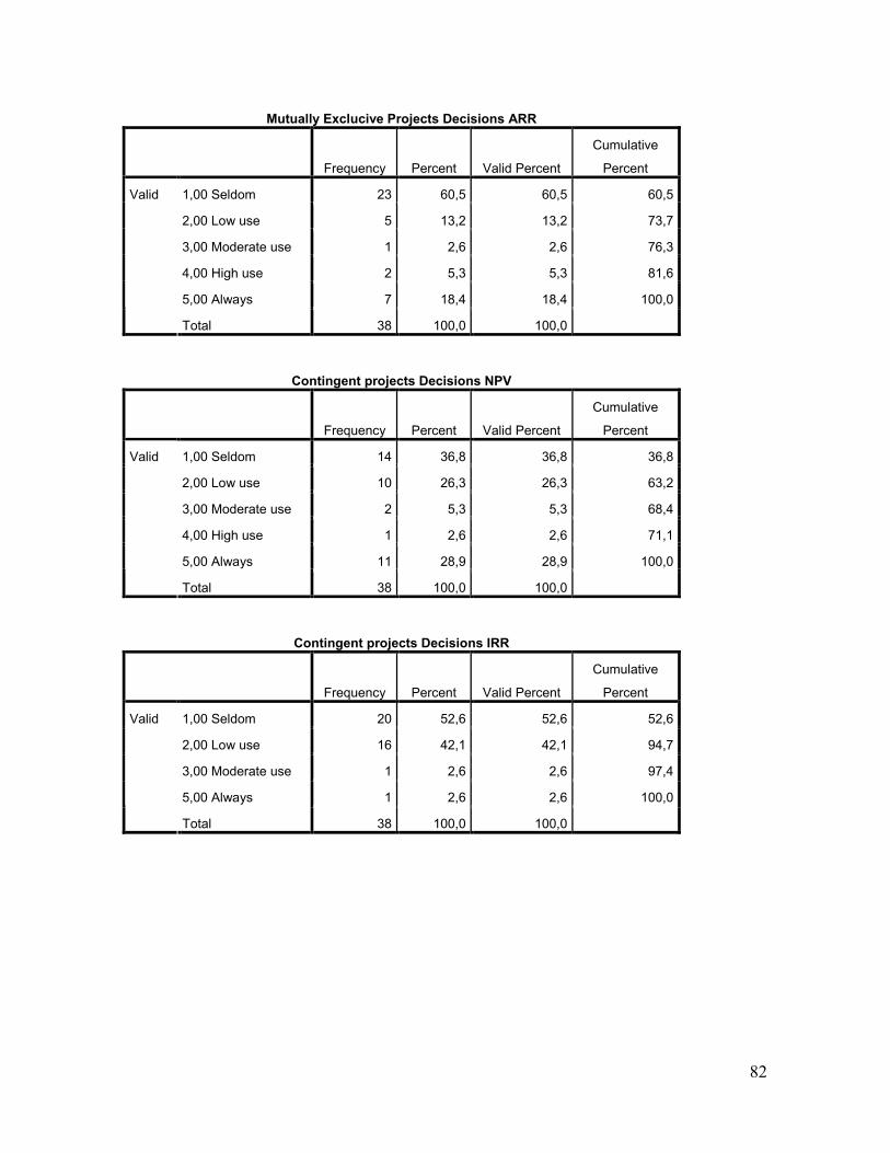
82

Mutually Exclucive Projects Decisions ARR

Frequency Percent Valid Percent

Cumulative

Percent

1,00 Seldom 23 60,5 60,5 60,5

2,00 Low use 5 13,2 13,2 73,7

3,00 Moderate use 1 2,6 2,6 76,3

4,00 High use 2 5,3 5,3 81,6

5,00 Always 7 18,4 18,4 100,0

Valid

Total 38 100,0 100,0

Contingent projects Decisions NPV

Frequency Percent Valid Percent

Cumulative

Percent

1,00 Seldom 14 36,8 36,8 36,8

2,00 Low use 10 26,3 26,3 63,2

3,00 Moderate use 2 5,3 5,3 68,4

4,00 High use 1 2,6 2,6 71,1

5,00 Always 11 28,9 28,9 100,0

Valid

Total 38 100,0 100,0

Contingent projects Decisions IRR

Frequency Percent Valid Percent

Cumulative

Percent

1,00 Seldom 20 52,6 52,6 52,6

2,00 Low use 16 42,1 42,1 94,7

3,00 Moderate use 1 2,6 2,6 97,4

5,00 Always 1 2,6 2,6 100,0

Valid

Total 38 100,0 100,0

83

Contingent projects Decisions PI

Frequency Percent Valid Percent

Cumulative

Percent

1,00 Seldom 17 44,7 44,7 44,7

2,00 Low use 9 23,7 23,7 68,4

3,00 Moderate use 2 5,3 5,3 73,7

4,00 High use 1 2,6 2,6 76,3

5,00 Always 9 23,7 23,7 100,0

Valid

Total 38 100,0 100,0

Contingent projects Decisions PBP

Frequency Percent Valid Percent

Cumulative

Percent

1,00 Seldom 12 31,6 31,6 31,6

2,00 Low use 2 5,3 5,3 36,8

3,00 Moderate use 3 7,9 7,9 44,7

4,00 High use 8 21,1 21,1 65,8

5,00 Always 13 34,2 34,2 100,0

Valid

Total 38 100,0 100,0

Contingent projects Decisions ARR

Frequency Percent Valid Percent

Cumulative

Percent

1,00 Seldom 23 60,5 60,5 60,5

2,00 Low use 5 13,2 13,2 73,7

3,00 Moderate use 1 2,6 2,6 76,3

4,00 High use 2 5,3 5,3 81,6

5,00 Always 7 18,4 18,4 100,0

Valid

Total 38 100,0 100,0

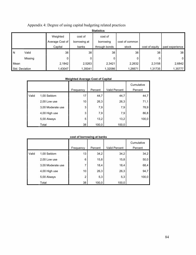
84

Appendix 4: Degree of using capital budgeting related practices

Statistics

Weighted

Average Cost of

Capital

cost of

borrowing at

banks

cost of

borrowing

through bonds

cost of common

stock cost of equity past experience

Valid 38 38 38 38 38 38 N

Missing 0 0 0 0 0 0

Mean 2,1842 2,5263 2,3421 2,2632 2,3158 2,6842

Std. Deviation 1,43047 1,35041 1,32086 1,26671 1,31735 1,35777

Weighted Average Cost of Capital

Frequency Percent Valid Percent

Cumulative

Percent

1,00 Seldom 17 44,7 44,7 44,7

2,00 Low use 10 26,3 26,3 71,1

3,00 Moderate use 3 7,9 7,9 78,9

4,00 High use 3 7,9 7,9 86,8

5,00 Always 5 13,2 13,2 100,0

Valid

Total 38 100,0 100,0

cost of borrowing at banks

Frequency Percent Valid Percent

Cumulative

Percent

1,00 Seldom 13 34,2 34,2 34,2

2,00 Low use 6 15,8 15,8 50,0

3,00 Moderate use 7 18,4 18,4 68,4

4,00 High use 10 26,3 26,3 94,7

5,00 Always 2 5,3 5,3 100,0

Valid

Total 38 100,0 100,0

85

cost of borrowing through bonds

Frequency Percent Valid Percent

Cumulative

Percent

1,00 Seldom 15 39,5 39,5 39,5

2,00 Low use 7 18,4 18,4 57,9

3,00 Moderate use 5 13,2 13,2 71,1

4,00 High use 10 26,3 26,3 97,4

5,00 Always 1 2,6 2,6 100,0

Valid

Total 38 100,0 100,0

cost of common stock

Frequency Percent Valid Percent

Cumulative

Percent

1,00 Seldom 16 42,1 42,1 42,1

2,00 Low use 5 13,2 13,2 55,3

3,00 Moderate use 9 23,7 23,7 78,9

4,00 High use 7 18,4 18,4 97,4

5,00 Always 1 2,6 2,6 100,0

Valid

Total 38 100,0 100,0

cost of equity

Frequency Percent Valid Percent

Cumulative

Percent

1,00 Seldom 16 42,1 42,1 42,1

2,00 Low use 4 10,5 10,5 52,6

3,00 Moderate use 10 26,3 26,3 78,9

4,00 High use 6 15,8 15,8 94,7

5,00 Always 2 5,3 5,3 100,0

Valid

Total 38 100,0 100,0

86

past experience

Frequency Percent Valid Percent

Cumulative

Percent

1,00 Seldom 10 26,3 26,3 26,3

2,00 Low use 8 21,1 21,1 47,4

3,00 Moderate use 8 21,1 21,1 68,4

4,00 High use 8 21,1 21,1 89,5

5,00 Always 4 10,5 10,5 100,0

Valid

Total 38 100,0 100,0

Statistics

probabili

ty

distributi

on

simulati

on

analysis decision tree

sensetivity

analysis

risk

adjustment

cash flow

risk

adjustme

nt PBP

risk

adjustm

ent

discount

rate

subjective

judgment

Valid 38 38 38 38 38 38 38 38 N

Missing 0 0 0 0 0 0 0 0

Mean 2,4211 1,8158 1,5263 2,0263 2,3421 2,8947 2,6579 2,8421

Std. Deviation 1,57053 1,08691 ,97916 1,40437 1,25798 1,39089 1,43840 1,30542

probability distribution

Frequency Percent Valid Percent

Cumulative

Percent

1,00 Seldom 17 44,7 44,7 44,7

2,00 Low use 6 15,8 15,8 60,5

3,00 Moderate use 3 7,9 7,9 68,4

4,00 High use 6 15,8 15,8 84,2

5,00 Always 6 15,8 15,8 100,0

Valid

Total 38 100,0 100,0

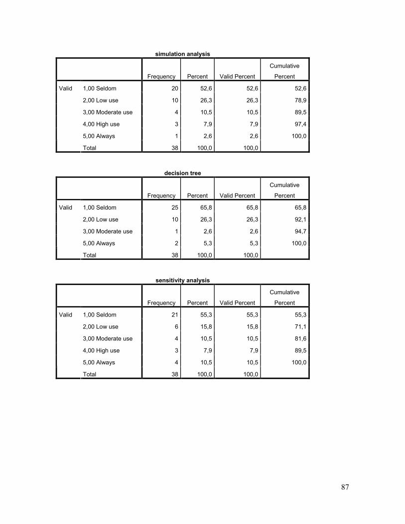
87

simulation analysis

Frequency Percent Valid Percent

Cumulative

Percent

1,00 Seldom 20 52,6 52,6 52,6

2,00 Low use 10 26,3 26,3 78,9

3,00 Moderate use 4 10,5 10,5 89,5

4,00 High use 3 7,9 7,9 97,4

5,00 Always 1 2,6 2,6 100,0

Valid

Total 38 100,0 100,0

decision tree

Frequency Percent Valid Percent

Cumulative

Percent

1,00 Seldom 25 65,8 65,8 65,8

2,00 Low use 10 26,3 26,3 92,1

3,00 Moderate use 1 2,6 2,6 94,7

5,00 Always 2 5,3 5,3 100,0

Valid

Total 38 100,0 100,0

sensitivity analysis

Frequency Percent Valid Percent

Cumulative

Percent

1,00 Seldom 21 55,3 55,3 55,3

2,00 Low use 6 15,8 15,8 71,1

3,00 Moderate use 4 10,5 10,5 81,6

4,00 High use 3 7,9 7,9 89,5

5,00 Always 4 10,5 10,5 100,0

Valid

Total 38 100,0 100,0

88

risk adjustment cash flow

Frequency Percent Valid Percent

Cumulative

Percent

1,00 Seldom 15 39,5 39,5 39,5

2,00 Low use 5 13,2 13,2 52,6

3,00 Moderate use 8 21,1 21,1 73,7

4,00 High use 10 26,3 26,3 100,0

Valid

Total 38 100,0 100,0

risk adjustment PBP

Frequency Percent Valid Percent

Cumulative

Percent

1,00 Seldom 11 28,9 28,9 28,9

2,00 Low use 3 7,9 7,9 36,8

3,00 Moderate use 5 13,2 13,2 50,0

4,00 High use 17 44,7 44,7 94,7

5,00 Always 2 5,3 5,3 100,0

Valid

Total 38 100,0 100,0

risk adjustment discount rate

Frequency Percent Valid Percent

Cumulative

Percent

1,00 Seldom 14 36,8 36,8 36,8

2,00 Low use 3 7,9 7,9 44,7

3,00 Moderate use 5 13,2 13,2 57,9

4,00 High use 14 36,8 36,8 94,7

5,00 Always 2 5,3 5,3 100,0

Valid

Total 38 100,0 100,0

89

subjective judgment

Frequency Percent Valid Percent

Cumulative

Percent

1,00 Seldom 9 23,7 23,7 23,7

2,00 Low use 6 15,8 15,8 39,5

3,00 Moderate use 7 18,4 18,4 57,9

4,00 High use 14 36,8 36,8 94,7

5,00 Always 2 5,3 5,3 100,0

Valid

Total 38 100,0 100,0

scenario projection

Frequency Percent Valid Percent

Cumulative

Percent

1,00 Seldom 24 63,2 63,2 63,2

2,00 Low use 7 18,4 18,4 81,6

3,00 Moderate use 3 7,9 7,9 89,5

4,00 High use 3 7,9 7,9 97,4

5,00 Always 1 2,6 2,6 100,0

Valid

Total 38 100,0 100,0

jury of executive opinion

Frequency Percent Valid Percent

Cumulative

Percent

1,00 Seldom 21 55,3 55,3 55,3

2,00 Low use 4 10,5 10,5 65,8

3,00 Moderate use 1 2,6 2,6 68,4

4,00 High use 11 28,9 28,9 97,4

5,00 Always 1 2,6 2,6 100,0

Valid

Total 38 100,0 100,0

90

nominal group technique

Frequency Percent Valid Percent

Cumulative

Percent

1,00 Seldom 23 60,5 60,5 60,5

2,00 Low use 7 18,4 18,4 78,9

3,00 Moderate use 3 7,9 7,9 86,8

4,00 High use 4 10,5 10,5 97,4

5,00 Always 1 2,6 2,6 100,0

Valid

Total 38 100,0 100,0

delphi method

Frequency Percent Valid Percent

Cumulative

Percent

1,00 Seldom 29 76,3 76,3 76,3

2,00 Low use 8 21,1 21,1 97,4

3,00 Moderate use 1 2,6 2,6 100,0

Valid

Total 38 100,0 100,0

moving averages

Frequency Percent Valid Percent

Cumulative

Percent

1,00 Seldom 25 65,8 65,8 65,8

2,00 Low use 8 21,1 21,1 86,8

3,00 Moderate use 4 10,5 10,5 97,4

5,00 Always 1 2,6 2,6 100,0

Valid

Total 38 100,0 100,0

91

time trend projection

Frequency Percent Valid Percent

Cumulative

Percent

1,00 Seldom 21 55,3 55,3 55,3

2,00 Low use 11 28,9 28,9 84,2

3,00 Moderate use 4 10,5 10,5 94,7

4,00 High use 1 2,6 2,6 97,4

5,00 Always 1 2,6 2,6 100,0

Valid

Total 38 100,0 100,0

multiple regression analysis

Frequency Percent Valid Percent

Cumulative

Percent

1,00 Seldom 18 47,4 47,4 47,4

2,00 Low use 5 13,2 13,2 60,5

3,00 Moderate use 5 13,2 13,2 73,7

4,00 High use 8 21,1 21,1 94,7

5,00 Always 2 5,3 5,3 100,0

Valid

Total 38 100,0 100,0

simple regression analysis

Frequency Percent Valid Percent

Cumulative

Percent

1,00 Seldom 19 50,0 50,0 50,0

2,00 Low use 4 10,5 10,5 60,5

3,00 Moderate use 5 13,2 13,2 73,7

4,00 High use 7 18,4 18,4 92,1

5,00 Always 3 7,9 7,9 100,0

Valid

Total 38 100,0 100,0

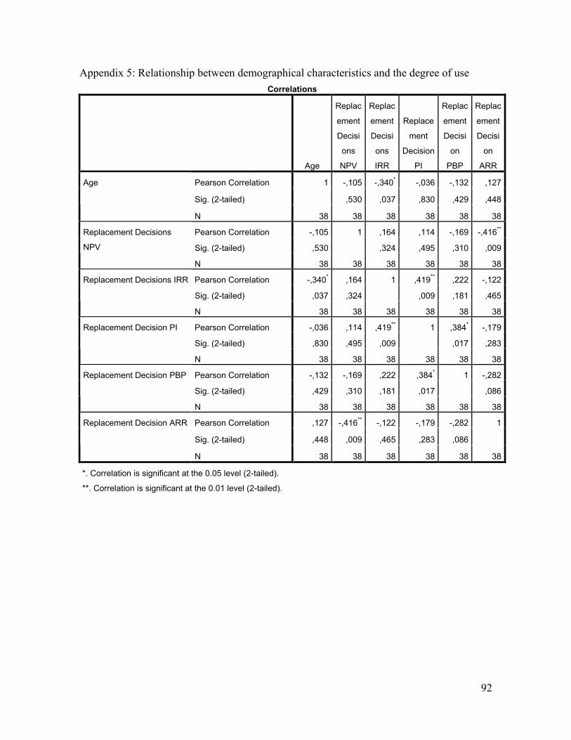
92

Appendix 5: Relationship between demographical characteristics and the degree of use

Correlations

Age

Replac

ement

Decisi

ons

NPV

Replac

ement

Decisi

ons

IRR

Replace

ment

Decision

PI

Replac

ement

Decisi

on

PBP

Replac

ement

Decisi

on

ARR

Pearson Correlation 1 -,105 -,340* -,036 -,132 ,127

Sig. (2-tailed) ,530 ,037 ,830 ,429 ,448

Age

N 38 38 38 38 38 38

Pearson Correlation -,105 1 ,164 ,114 -,169 -,416**

Sig. (2-tailed) ,530 ,324 ,495 ,310 ,009

Replacement Decisions

NPV

N 38 38 38 38 38 38

Pearson Correlation -,340* ,164 1 ,419

** ,222 -,122

Sig. (2-tailed) ,037 ,324 ,009 ,181 ,465

Replacement Decisions IRR

N 38 38 38 38 38 38

Pearson Correlation -,036 ,114 ,419** 1 ,384

* -,179

Sig. (2-tailed) ,830 ,495 ,009 ,017 ,283

Replacement Decision PI

N 38 38 38 38 38 38

Pearson Correlation -,132 -,169 ,222 ,384* 1 -,282

Sig. (2-tailed) ,429 ,310 ,181 ,017 ,086

Replacement Decision PBP

N 38 38 38 38 38 38

Pearson Correlation ,127 -,416** -,122 -,179 -,282 1

Sig. (2-tailed) ,448 ,009 ,465 ,283 ,086

Replacement Decision ARR

N 38 38 38 38 38 38

*. Correlation is significant at the 0.05 level (2-tailed).

**. Correlation is significant at the 0.01 level (2-tailed).

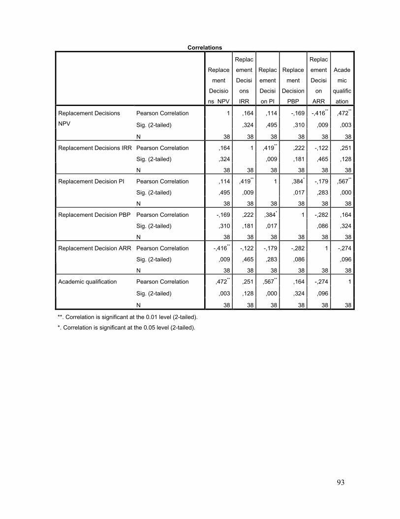
93

Correlations

Replace

ment

Decisio

ns NPV

Replac

ement

Decisi

ons

IRR

Replac

ement

Decisi

on PI

Replace

ment

Decision

PBP

Replac

ement

Decisi

on

ARR

Acade

mic

qualific

ation

Pearson Correlation 1 ,164 ,114 -,169 -,416** ,472

**

Sig. (2-tailed) ,324 ,495 ,310 ,009 ,003

Replacement Decisions

NPV

N 38 38 38 38 38 38

Pearson Correlation ,164 1 ,419** ,222 -,122 ,251

Sig. (2-tailed) ,324 ,009 ,181 ,465 ,128

Replacement Decisions IRR

N 38 38 38 38 38 38

Pearson Correlation ,114 ,419** 1 ,384

* -,179 ,567

**

Sig. (2-tailed) ,495 ,009 ,017 ,283 ,000

Replacement Decision PI

N 38 38 38 38 38 38

Pearson Correlation -,169 ,222 ,384* 1 -,282 ,164

Sig. (2-tailed) ,310 ,181 ,017 ,086 ,324

Replacement Decision PBP

N 38 38 38 38 38 38

Pearson Correlation -,416** -,122 -,179 -,282 1 -,274

Sig. (2-tailed) ,009 ,465 ,283 ,086 ,096

Replacement Decision ARR

N 38 38 38 38 38 38

Pearson Correlation ,472** ,251 ,567

** ,164 -,274 1

Sig. (2-tailed) ,003 ,128 ,000 ,324 ,096

Academic qualification

N 38 38 38 38 38 38

**. Correlation is significant at the 0.01 level (2-tailed).

*. Correlation is significant at the 0.05 level (2-tailed).

94

Correlations

Replac

ement

Decisi

ons

NPV

Replace

ment

Decision

s IRR

Replac

ement

Decisi

on PI

Replace

ment

Decision

PBP

Replac

ement

Decisi

on

ARR

Experi

ence

Pearson Correlation 1 ,164 ,114 -,169 -,416** -,206

Sig. (2-tailed) ,324 ,495 ,310 ,009 ,214

Replacement Decisions

NPV

N 38 38 38 38 38 38

Pearson Correlation ,164 1 ,419** ,222 -,122 -,241

Sig. (2-tailed) ,324 ,009 ,181 ,465 ,145

Replacement Decisions

IRR

N 38 38 38 38 38 38

Pearson Correlation ,114 ,419** 1 ,384

* -,179 -,198

Sig. (2-tailed) ,495 ,009 ,017 ,283 ,233

Replacement Decision

PI

N 38 38 38 38 38 38

Pearson Correlation -,169 ,222 ,384* 1 -,282 -,119

Sig. (2-tailed) ,310 ,181 ,017 ,086 ,476

Replacement Decision

PBP

N 38 38 38 38 38 38

Pearson Correlation -,416** -,122 -,179 -,282 1 ,169

Sig. (2-tailed) ,009 ,465 ,283 ,086 ,311

Replacement Decision

ARR

N 38 38 38 38 38 38

Pearson Correlation -,206 -,241 -,198 -,119 ,169 1

Sig. (2-tailed) ,214 ,145 ,233 ,476 ,311

Experience

N 38 38 38 38 38 38

**. Correlation is significant at the 0.01 level (2-tailed).

*. Correlation is significant at the 0.05 level (2-tailed).

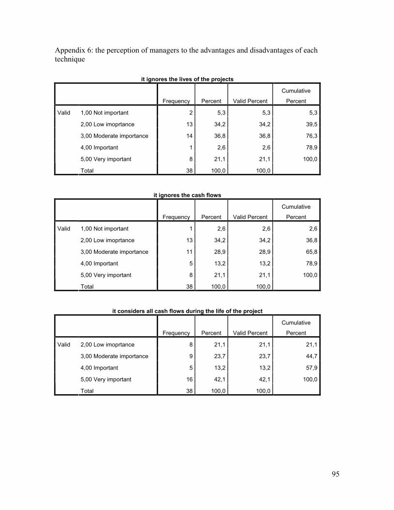
95

Appendix 6: the perception of managers to the advantages and disadvantages of each technique

it ignores the lives of the projects

Frequency Percent Valid Percent

Cumulative

Percent

1,00 Not important 2 5,3 5,3 5,3

2,00 Low imoprtance 13 34,2 34,2 39,5

3,00 Moderate importance 14 36,8 36,8 76,3

4,00 Important 1 2,6 2,6 78,9

5,00 Very important 8 21,1 21,1 100,0

Valid

Total 38 100,0 100,0

it ignores the cash flows

Frequency Percent Valid Percent

Cumulative

Percent

1,00 Not important 1 2,6 2,6 2,6

2,00 Low imoprtance 13 34,2 34,2 36,8

3,00 Moderate importance 11 28,9 28,9 65,8

4,00 Important 5 13,2 13,2 78,9

5,00 Very important 8 21,1 21,1 100,0

Valid

Total 38 100,0 100,0

it considers all cash flows during the life of the project

Frequency Percent Valid Percent

Cumulative

Percent

2,00 Low imoprtance 8 21,1 21,1 21,1

3,00 Moderate importance 9 23,7 23,7 44,7

4,00 Important 5 13,2 13,2 57,9

5,00 Very important 16 42,1 42,1 100,0

Valid

Total 38 100,0 100,0

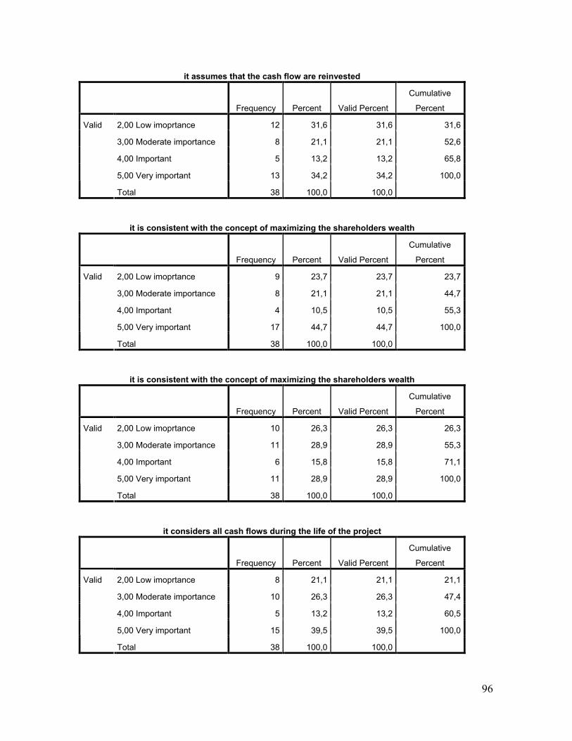
96

it assumes that the cash flow are reinvested

Frequency Percent Valid Percent

Cumulative

Percent

2,00 Low imoprtance 12 31,6 31,6 31,6

3,00 Moderate importance 8 21,1 21,1 52,6

4,00 Important 5 13,2 13,2 65,8

5,00 Very important 13 34,2 34,2 100,0

Valid

Total 38 100,0 100,0

it is consistent with the concept of maximizing the shareholders wealth

Frequency Percent Valid Percent

Cumulative

Percent

2,00 Low imoprtance 9 23,7 23,7 23,7

3,00 Moderate importance 8 21,1 21,1 44,7

4,00 Important 4 10,5 10,5 55,3

5,00 Very important 17 44,7 44,7 100,0

Valid

Total 38 100,0 100,0

it is consistent with the concept of maximizing the shareholders wealth

Frequency Percent Valid Percent

Cumulative

Percent

2,00 Low imoprtance 10 26,3 26,3 26,3

3,00 Moderate importance 11 28,9 28,9 55,3

4,00 Important 6 15,8 15,8 71,1

5,00 Very important 11 28,9 28,9 100,0

Valid

Total 38 100,0 100,0

it considers all cash flows during the life of the project

Frequency Percent Valid Percent

Cumulative

Percent

2,00 Low imoprtance 8 21,1 21,1 21,1

3,00 Moderate importance 10 26,3 26,3 47,4

4,00 Important 5 13,2 13,2 60,5

5,00 Very important 15 39,5 39,5 100,0

Valid

Total 38 100,0 100,0

97

it gives a relative measure to rank projects according to their profitability

Frequency Percent Valid Percent

Cumulative

Percent

2,00 Low imoprtance 12 31,6 31,6 31,6

3,00 Moderate importance 12 31,6 31,6 63,2

4,00 Important 2 5,3 5,3 68,4

5,00 Very important 12 31,6 31,6 100,0

Valid

Total 38 100,0 100,0

it assumes that the discount rate is already known

Frequency Percent Valid Percent

Cumulative

Percent

1,00 Not important 3 7,9 7,9 7,9

2,00 Low imoprtance 9 23,7 23,7 31,6

3,00 Moderate importance 21 55,3 55,3 86,8

4,00 Important 3 7,9 7,9 94,7

5,00 Very important 2 5,3 5,3 100,0

Valid

Total 38 100,0 100,0

it can not handle non- conventional cash flows

Frequency Percent Valid Percent

Cumulative

Percent

2,00 Low imoprtance 9 23,7 23,7 23,7

3,00 Moderate importance 24 63,2 63,2 86,8

4,00 Important 4 10,5 10,5 97,4

5,00 Very important 1 2,6 2,6 100,0

Valid

Total 38 100,0 100,0

financing type decision may misintrepret the calculations results

Frequency Percent Valid Percent

Cumulative

Percent

1,00 Not important 2 5,3 5,3 5,3

2,00 Low imoprtance 8 21,1 21,1 26,3

3,00 Moderate importance 22 57,9 57,9 84,2

4,00 Important 3 7,9 7,9 92,1

Valid

5,00 Very important 3 7,9 7,9 100,0

98

financing type decision may misintrepret the calculations results

Frequency Percent Valid Percent

Cumulative

Percent

1,00 Not important 2 5,3 5,3 5,3

2,00 Low imoprtance 8 21,1 21,1 26,3

3,00 Moderate importance 22 57,9 57,9 84,2

4,00 Important 3 7,9 7,9 92,1

5,00 Very important 3 7,9 7,9 100,0

Total 38 100,0 100,0

it does not consider the size of the investment

Frequency Percent Valid Percent

Cumulative

Percent

1,00 Not important 1 2,6 2,6 2,6

2,00 Low imoprtance 9 23,7 23,7 26,3

3,00 Moderate importance 25 65,8 65,8 92,1

4,00 Important 3 7,9 7,9 100,0

Valid

Total 38 100,0 100,0

it does not consider the size of the projects when it ranks them

Frequency Percent Valid Percent

Cumulative

Percent

1,00 Not important 2 5,3 5,3 5,3

2,00 Low imoprtance 10 26,3 26,3 31,6

3,00 Moderate importance 23 60,5 60,5 92,1

4,00 Important 2 5,3 5,3 97,4

5,00 Very important 1 2,6 2,6 100,0

Valid

Total 38 100,0 100,0

99

Easy to calculate and understand

Frequency Percent Valid Percent

Cumulative

Percent

1,00 Not important 1 2,6 2,6 2,6

2,00 Low imoprtance 9 23,7 23,7 26,3

3,00 Moderate importance 5 13,2 13,2 39,5

4,00 Important 6 15,8 15,8 55,3

5,00 Very important 17 44,7 44,7 100,0

Valid

Total 38 100,0 100,0

it does not consider the time value of money

Frequency Percent Valid Percent

Cumulative

Percent

1,00 Not important 1 2,6 2,6 2,6

2,00 Low imoprtance 10 26,3 26,3 28,9

3,00 Moderate importance 12 31,6 31,6 60,5

4,00 Important 5 13,2 13,2 73,7

5,00 Very important 10 26,3 26,3 100,0

Valid

Total 38 100,0 100,0

it considers all incomes in the project's life

Frequency Percent Valid Percent

Cumulative

Percent

2,00 Low imoprtance 7 18,4 18,4 18,4

3,00 Moderate importance 9 23,7 23,7 42,1

4,00 Important 8 21,1 21,1 63,2

5,00 Very important 14 36,8 36,8 100,0

Valid

Total 38 100,0 100,0

100

it does not consider the time value of money

Frequency Percent Valid Percent

Cumulative

Percent

1,00 Not important 1 2,6 2,6 2,6

2,00 Low imoprtance 13 34,2 34,2 36,8

3,00 Moderate importance 10 26,3 26,3 63,2

4,00 Important 4 10,5 10,5 73,7

5,00 Very important 10 26,3 26,3 100,0

Valid

Total 38 100,0 100,0

it does not consider the cash flow after the PBP

Frequency Percent Valid Percent

Cumulative

Percent

1,00 Not important 2 5,3 5,3 5,3

2,00 Low imoprtance 10 26,3 26,3 31,6

3,00 Moderate importance 13 34,2 34,2 65,8

4,00 Important 6 15,8 15,8 81,6

5,00 Very important 7 18,4 18,4 100,0

Valid

Total 38 100,0 100,0

it does not reflect the profitability of the project

Frequency Percent Valid Percent

Cumulative

Percent

1,00 Not important 1 2,6 2,6 2,6

2,00 Low imoprtance 11 28,9 28,9 31,6

3,00 Moderate importance 12 31,6 31,6 63,2

4,00 Important 6 15,8 15,8 78,9

5,00 Very important 8 21,1 21,1 100,0

Valid

Total 38 100,0 100,0

101

it considers the time value of money

Frequency Percent Valid Percent

Cumulative

Percent

2,00 Low imoprtance 8 21,1 21,1 21,1

3,00 Moderate importance 8 21,1 21,1 42,1

4,00 Important 3 7,9 7,9 50,0

5,00 Very important 19 50,0 50,0 100,0

Valid

Total 38 100,0 100,0

it handles non conventional cash flows

Frequency Percent Valid Percent

Cumulative

Percent

1,00 Not important 1 2,6 2,6 2,6

2,00 Low imoprtance 9 23,7 23,7 26,3

3,00 Moderate importance 10 26,3 26,3 52,6

4,00 Important 8 21,1 21,1 73,7

5,00 Very important 10 26,3 26,3 100,0

Valid

Total 38 100,0 100,0

it gives a percenatge measure

Frequency Percent Valid Percent

Cumulative

Percent

2,00 Low imoprtance 11 28,9 28,9 28,9

3,00 Moderate importance 14 36,8 36,8 65,8

4,00 Important 6 15,8 15,8 81,6

5,00 Very important 7 18,4 18,4 100,0

Valid

Total 38 100,0 100,0

it considers the time value of money

Frequency Percent Valid Percent

Cumulative

Percent

2,00 Low imoprtance 7 18,4 18,4 18,4

3,00 Moderate importance 11 28,9 28,9 47,4

4,00 Important 5 13,2 13,2 60,5

Valid

5,00 Very important 15 39,5 39,5 100,0

102

it considers the time value of money

Frequency Percent Valid Percent

Cumulative

Percent

2,00 Low imoprtance 7 18,4 18,4 18,4

3,00 Moderate importance 11 28,9 28,9 47,4

4,00 Important 5 13,2 13,2 60,5

5,00 Very important 15 39,5 39,5 100,0

Total 38 100,0 100,0

it does not give a percentage measure

Frequency Percent Valid Percent

Cumulative

Percent

1,00 Not important 2 5,3 5,3 5,3

2,00 Low imoprtance 10 26,3 26,3 31,6

3,00 Moderate importance 22 57,9 57,9 89,5

4,00 Important 2 5,3 5,3 94,7

5,00 Very important 2 5,3 5,3 100,0

Valid

Total 38 100,0 100,0

it considers all cash flows during the life of the project

Frequency Percent Valid Percent

Cumulative

Percent

2,00 Low imoprtance 11 28,9 28,9 28,9

3,00 Moderate importance 8 21,1 21,1 50,0

4,00 Important 9 23,7 23,7 73,7

5,00 Very important 10 26,3 26,3 100,0

Valid

Total 38 100,0 100,0

it considers the time value of money

Frequency Percent Valid Percent

Cumulative

Percent

2,00 Low imoprtance 10 26,3 26,3 26,3

3,00 Moderate importance 9 23,7 23,7 50,0

4,00 Important 5 13,2 13,2 63,2

5,00 Very important 14 36,8 36,8 100,0

Valid

Total 38 100,0 100,0

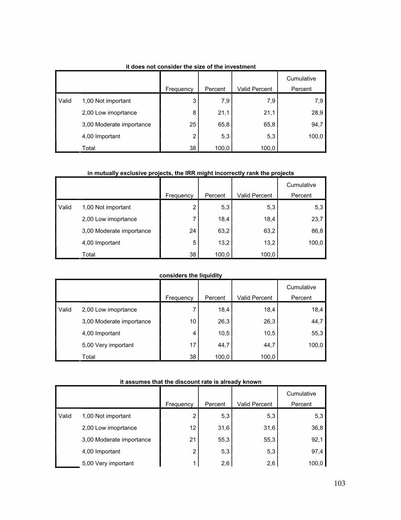
103

it does not consider the size of the investment

Frequency Percent Valid Percent

Cumulative

Percent

1,00 Not important 3 7,9 7,9 7,9

2,00 Low imoprtance 8 21,1 21,1 28,9

3,00 Moderate importance 25 65,8 65,8 94,7

4,00 Important 2 5,3 5,3 100,0

Valid

Total 38 100,0 100,0

in mutually exclusive projects, the IRR might incorrectly rank the projects

Frequency Percent Valid Percent

Cumulative

Percent

1,00 Not important 2 5,3 5,3 5,3

2,00 Low imoprtance 7 18,4 18,4 23,7

3,00 Moderate importance 24 63,2 63,2 86,8

4,00 Important 5 13,2 13,2 100,0

Valid

Total 38 100,0 100,0

considers the liquidity

Frequency Percent Valid Percent

Cumulative

Percent

2,00 Low imoprtance 7 18,4 18,4 18,4

3,00 Moderate importance 10 26,3 26,3 44,7

4,00 Important 4 10,5 10,5 55,3

5,00 Very important 17 44,7 44,7 100,0

Valid

Total 38 100,0 100,0

it assumes that the discount rate is already known

Frequency Percent Valid Percent

Cumulative

Percent

1,00 Not important 2 5,3 5,3 5,3

2,00 Low imoprtance 12 31,6 31,6 36,8

3,00 Moderate importance 21 55,3 55,3 92,1

4,00 Important 2 5,3 5,3 97,4

Valid

5,00 Very important 1 2,6 2,6 100,0

104

it assumes that the discount rate is already known

Frequency Percent Valid Percent

Cumulative

Percent

1,00 Not important 2 5,3 5,3 5,3

2,00 Low imoprtance 12 31,6 31,6 36,8

3,00 Moderate importance 21 55,3 55,3 92,1

4,00 Important 2 5,3 5,3 97,4

5,00 Very important 1 2,6 2,6 100,0

Total 38 100,0 100,0

Easy to calculate and understand

Frequency Percent Valid Percent

Cumulative

Percent

1,00 Not important 1 2,6 2,6 2,6

2,00 Low imoprtance 7 18,4 18,4 21,1

3,00 Moderate importance 8 21,1 21,1 42,1

4,00 Important 5 13,2 13,2 55,3

5,00 Very important 17 44,7 44,7 100,0

Valid

Total 38 100,0 100,0

105

Appendix 7: The relationship between the perception of the respondents to the advantages and disadvantages of the techniques and their use

Chi-Square Tests

Value df

Asymp. Sig. (2-

sided)

Pearson Chi-Square 26,727a 12 ,008

Likelihood Ratio 34,314 12 ,001

Linear-by-Linear Association 19,535 1 ,000

N of Valid Cases 38

a. 18 cells (90,0%) have expected count less than 5. The minimum

expected count is ,16.

Chi-Square Tests

Value df

Asymp. Sig. (2-

sided)

Pearson Chi-Square 31,009a 12 ,002

Likelihood Ratio 36,723 12 ,000

Linear-by-Linear Association 19,089 1 ,000

N of Valid Cases 38

a. 19 cells (95,0%) have expected count less than 5. The minimum

expected count is ,26.

Chi-Square Tests

Value df

Asymp. Sig. (2-

sided)

Pearson Chi-Square 42,739a 12 ,000

Likelihood Ratio 44,411 12 ,000

Linear-by-Linear Association 19,296 1 ,000

N of Valid Cases 38

a. 20 cells (100,0%) have expected count less than 5. The minimum

expected count is ,26.

106

Chi-Square Tests

Value df

Asymp. Sig. (2-

sided)

Pearson Chi-Square 37,176a 16 ,002

Likelihood Ratio 44,889 16 ,000

Linear-by-Linear Association 16,793 1 ,000

N of Valid Cases 38

a. 25 cells (100,0%) have expected count less than 5. The minimum

expected count is ,05.

Chi-Square Tests

Value df

Asymp. Sig. (2-

sided)

Pearson Chi-Square 22,992a 12 ,028

Likelihood Ratio 28,437 12 ,005

Linear-by-Linear Association 16,520 1 ,000

N of Valid Cases 38

a. 19 cells (95,0%) have expected count less than 5. The minimum

expected count is ,21.

Chi-Square Tests

Value df

Asymp. Sig. (2-

sided)

Pearson Chi-Square 34,951a 16 ,004

Likelihood Ratio 29,992 16 ,018

Linear-by-Linear Association ,434 1 ,510

N of Valid Cases 38

a. 22 cells (88,0%) have expected count less than 5. The minimum

expected count is ,11.

Chi-Square Tests

Value df

Asymp. Sig. (2-

sided)

Pearson Chi-Square 33,097a 16 ,007

Likelihood Ratio 26,178 16 ,052

Linear-by-Linear Association ,035 1 ,853

N of Valid Cases 38

107

Chi-Square Tests

Value df

Asymp. Sig. (2-

sided)

Pearson Chi-Square 33,097a 16 ,007

Likelihood Ratio 26,178 16 ,052

Linear-by-Linear Association ,035 1 ,853

N of Valid Cases 38

a. 23 cells (92,0%) have expected count less than 5. The minimum

expected count is ,11.

Chi-Square Tests

Value df

Asymp. Sig. (2-

sided)

Pearson Chi-Square 19,275a 12 ,082

Likelihood Ratio 19,332 12 ,081

Linear-by-Linear Association ,184 1 ,668

N of Valid Cases 38

a. 17 cells (85,0%) have expected count less than 5. The minimum

expected count is ,11.

Chi-Square Tests

Value df

Asymp. Sig. (2-

sided)

Pearson Chi-Square 5,881a 9 ,752

Likelihood Ratio 6,747 9 ,663

Linear-by-Linear Association 2,929 1 ,087

N of Valid Cases 38

a. 13 cells (81,3%) have expected count less than 5. The minimum

expected count is ,13.

Chi-Square Tests

Value df

Asymp. Sig. (2-

sided)

Pearson Chi-Square 10,573a 9 ,306

Likelihood Ratio 9,802 9 ,367

Linear-by-Linear Association ,597 1 ,440

N of Valid Cases 38

108

Chi-Square Tests

Value df

Asymp. Sig. (2-

sided)

Pearson Chi-Square 10,573a 9 ,306

Likelihood Ratio 9,802 9 ,367

Linear-by-Linear Association ,597 1 ,440

N of Valid Cases 38

a. 14 cells (87,5%) have expected count less than 5. The minimum

expected count is ,21.

Chi-Square Tests

Value df

Asymp. Sig. (2-

sided)

Pearson Chi-Square 10,025a 9 ,348

Likelihood Ratio 9,718 9 ,374

Linear-by-Linear Association 1,575 1 ,209

N of Valid Cases 38

a. 13 cells (81,3%) have expected count less than 5. The minimum

expected count is ,16.

Chi-Square Tests

Value df

Asymp. Sig. (2-

sided)

Pearson Chi-Square 18,685a 9 ,028

Likelihood Ratio 15,389 9 ,081

Linear-by-Linear Association ,597 1 ,440

N of Valid Cases 38

a. 13 cells (81,3%) have expected count less than 5. The minimum

expected count is ,16.

Chi-Square Tests

Value df

Asymp. Sig. (2-

sided)

Pearson Chi-Square 14,677a 9 ,100

Likelihood Ratio 16,011 9 ,067

Linear-by-Linear Association 1,220 1 ,269

N of Valid Cases 38

109

Chi-Square Tests

Value df

Asymp. Sig. (2-

sided)

Pearson Chi-Square 14,677a 9 ,100

Likelihood Ratio 16,011 9 ,067

Linear-by-Linear Association 1,220 1 ,269

N of Valid Cases 38

a. 14 cells (87,5%) have expected count less than 5. The minimum

expected count is ,03.

Chi-Square Tests

Value df

Asymp. Sig. (2-

sided)

Pearson Chi-Square 26,608a 12 ,009

Likelihood Ratio 22,745 12 ,030

Linear-by-Linear Association 7,723 1 ,005

N of Valid Cases 38

a. 18 cells (90,0%) have expected count less than 5. The minimum

expected count is ,05.

Chi-Square Tests

Value df

Asymp. Sig. (2-

sided)

Pearson Chi-Square 19,905a 9 ,019

Likelihood Ratio 22,263 9 ,008

Linear-by-Linear Association 11,960 1 ,001

N of Valid Cases 38

a. 14 cells (87,5%) have expected count less than 5. The minimum

expected count is ,05.

Chi-Square Tests

Value df

Asymp. Sig. (2-

sided)

Pearson Chi-Square 23,846a 9 ,005

Likelihood Ratio 18,404 9 ,031

Linear-by-Linear Association 7,622 1 ,006

N of Valid Cases 38

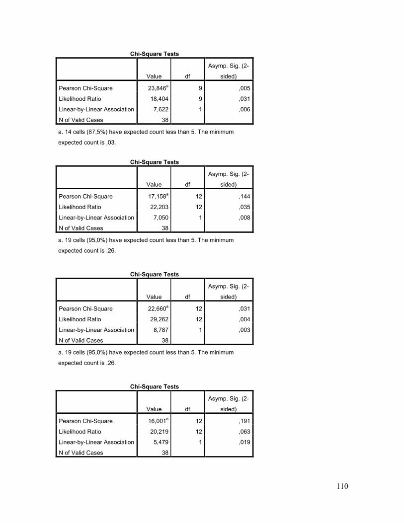
110

Chi-Square Tests

Value df

Asymp. Sig. (2-

sided)

Pearson Chi-Square 23,846a 9 ,005

Likelihood Ratio 18,404 9 ,031

Linear-by-Linear Association 7,622 1 ,006

N of Valid Cases 38

a. 14 cells (87,5%) have expected count less than 5. The minimum

expected count is ,03.

Chi-Square Tests

Value df

Asymp. Sig. (2-

sided)

Pearson Chi-Square 17,158a 12 ,144

Likelihood Ratio 22,203 12 ,035

Linear-by-Linear Association 7,050 1 ,008

N of Valid Cases 38

a. 19 cells (95,0%) have expected count less than 5. The minimum

expected count is ,26.

Chi-Square Tests

Value df

Asymp. Sig. (2-

sided)

Pearson Chi-Square 22,660a 12 ,031

Likelihood Ratio 29,262 12 ,004

Linear-by-Linear Association 8,787 1 ,003

N of Valid Cases 38

a. 19 cells (95,0%) have expected count less than 5. The minimum

expected count is ,26.

Chi-Square Tests

Value df

Asymp. Sig. (2-

sided)

Pearson Chi-Square 16,001a 12 ,191

Likelihood Ratio 20,219 12 ,063

Linear-by-Linear Association 5,479 1 ,019

N of Valid Cases 38

111

Chi-Square Tests

Value df

Asymp. Sig. (2-

sided)

Pearson Chi-Square 16,001a 12 ,191

Likelihood Ratio 20,219 12 ,063

Linear-by-Linear Association 5,479 1 ,019

N of Valid Cases 38

a. 17 cells (85,0%) have expected count less than 5. The minimum

expected count is ,11.

Chi-Square Tests

Value df

Asymp. Sig. (2-

sided)

Pearson Chi-Square 12,625a 16 ,700

Likelihood Ratio 14,159 16 ,587

Linear-by-Linear Association ,107 1 ,743

N of Valid Cases 38

a. 23 cells (92,0%) have expected count less than 5. The minimum

expected count is ,05.

Chi-Square Tests

Value df

Asymp. Sig. (2-

sided)

Pearson Chi-Square 9,320a 16 ,900

Likelihood Ratio 9,899 16 ,872

Linear-by-Linear Association ,657 1 ,418

N of Valid Cases 38

a. 23 cells (92,0%) have expected count less than 5. The minimum

expected count is ,05.

Chi-Square Tests

Value df

Asymp. Sig. (2-

sided)

Pearson Chi-Square 21,121a 12 ,049

Likelihood Ratio 23,755 12 ,022

Linear-by-Linear Association 11,898 1 ,001

N of Valid Cases 38

112

Chi-Square Tests

Value df

Asymp. Sig. (2-

sided)

Pearson Chi-Square 21,121a 12 ,049

Likelihood Ratio 23,755 12 ,022

Linear-by-Linear Association 11,898 1 ,001

N of Valid Cases 38

a. 19 cells (95,0%) have expected count less than 5. The minimum

expected count is ,21.

Chi-Square Tests

Value df

Asymp. Sig. (2-

sided)

Pearson Chi-Square 28,633a 16 ,027

Likelihood Ratio 22,029 16 ,142

Linear-by-Linear Association 7,039 1 ,008

N of Valid Cases 38

a. 24 cells (96,0%) have expected count less than 5. The minimum

expected count is ,05.

Chi-Square Tests

Value df

Asymp. Sig. (2-

sided)

Pearson Chi-Square 12,957a 16 ,676

Likelihood Ratio 13,765 16 ,616

Linear-by-Linear Association 1,536 1 ,215

N of Valid Cases 38

a. 25 cells (100,0%) have expected count less than 5. The minimum

expected count is ,05.

Chi-Square Tests

Value df

Asymp. Sig. (2-

sided)

Pearson Chi-Square 21,398a 16 ,164

Likelihood Ratio 24,220 16 ,085

Linear-by-Linear Association 2,170 1 ,141

N of Valid Cases 38

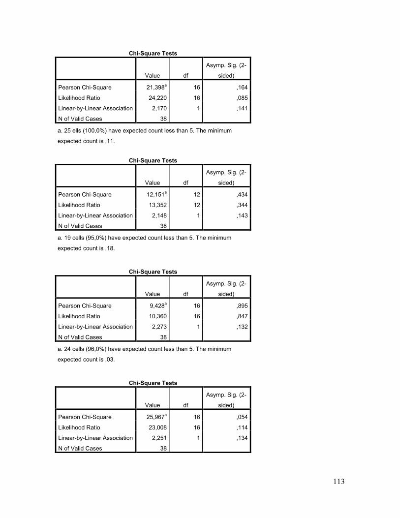
113

Chi-Square Tests

Value df

Asymp. Sig. (2-

sided)

Pearson Chi-Square 21,398a 16 ,164

Likelihood Ratio 24,220 16 ,085

Linear-by-Linear Association 2,170 1 ,141

N of Valid Cases 38

a. 25 ells (100,0%) have expected count less than 5. The minimum

expected count is ,11.

Chi-Square Tests

Value df

Asymp. Sig. (2-

sided)

Pearson Chi-Square 12,151a 12 ,434

Likelihood Ratio 13,352 12 ,344

Linear-by-Linear Association 2,148 1 ,143

N of Valid Cases 38

a. 19 cells (95,0%) have expected count less than 5. The minimum

expected count is ,18.

Chi-Square Tests

Value df

Asymp. Sig. (2-

sided)

Pearson Chi-Square 9,428a 16 ,895

Likelihood Ratio 10,360 16 ,847

Linear-by-Linear Association 2,273 1 ,132

N of Valid Cases 38

a. 24 cells (96,0%) have expected count less than 5. The minimum

expected count is ,03.

Chi-Square Tests

Value df

Asymp. Sig. (2-

sided)

Pearson Chi-Square 25,967a 16 ,054

Likelihood Ratio 23,008 16 ,114

Linear-by-Linear Association 2,251 1 ,134

N of Valid Cases 38

114

Chi-Square Tests

Value df

Asymp. Sig. (2-

sided)

Pearson Chi-Square 25,967a 16 ,054

Likelihood Ratio 23,008 16 ,114

Linear-by-Linear Association 2,251 1 ,134

N of Valid Cases 38

a. 22 cells (88,0%) have expected count less than 5. The minimum

expected count is ,03.

Chi-Square Tests

Value df

Asymp. Sig. (2-

sided)

Pearson Chi-Square 13,313a 16 ,650

Likelihood Ratio 13,040 16 ,670

Linear-by-Linear Association 1,254 1 ,263

N of Valid Cases 38

a. 23 cells (92,0%) have expected count less than 5. The minimum

expected count is ,03.

Chi-Square Tests

Value df

Asymp. Sig. (2-

sided)

Pearson Chi-Square 26,493a 16 ,047

Likelihood Ratio 24,678 16 ,076

Linear-by-Linear Association 1,883 1 ,170

N of Valid Cases 38

a. 23 cells (92,0%) have expected count less than 5. The minimum

expected count is ,03.

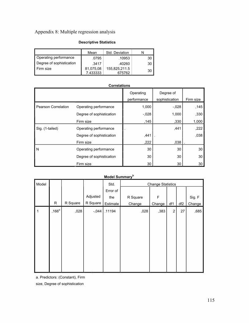
115

Appendix 8: Multiple regression analysis Descriptive Statistics

Mean Std. Deviation N

Operating performance .0795 .10953 30

Degree of sophistication .3417 .40260 30

Firm size 81,075,087.433333

155,825,211.5675762

30

Correlations

Operating

performance

Degree of

sophistication Firm size

Operating performance 1,000 -,028 ,145

Degree of sophistication -,028 1,000 ,330

Pearson Correlation

Firm size ,145 ,330 1,000

Operating performance . ,441 ,222

Degree of sophistication ,441 . ,038

Sig. (1-tailed)

Firm size ,222 ,038 .

Operating performance 30 30 30

Degree of sophistication 30 30 30

N

Firm size 30 30 30

Model Summaryb

Change Statistics Model

R R Square

Adjusted

R Square

Std.

Error of

the

Estimate

R Square

Change

F

Change df1 df2

Sig. F

Change

1 ,166a ,028 -,044 .11194 ,028 ,383 2 27 ,685

a. Predictors: (Constant), Firm

size, Degree of sophistication

116

Model Summaryb

Change Statistics Model

R R Square

Adjusted

R Square

Std.

Error of

the

Estimate

R Square

Change

F

Change df1 df2

Sig. F

Change

1 ,166a ,028 -,044 .11194 ,028 ,383 2 27 ,685

a. Predictors: (Constant), Firm

size, Degree of sophistication

b. Dependent Variable: Operating

performance

ANOVAb

Model Sum of Squares df Mean Square F Sig.

Regression ,010 2 ,005 ,383 ,685a

Residual ,338 27 ,013

1

Total ,348 29

a. Predictors: (Constant), Firm size, Degree of sophistication

b. Dependent Variable: Operating performance Coefficients(a)

Unstandardized Coefficients

Standardized Coefficients t Sig.

Model B Std. Error Beta B Std. Error

(Constant) .078 .028 2.820 .009

Degree of sophistication -.023 .055 -.085 -.425 .674

1

Firm size 1.22E-010 .000 .173 .862 .396

a Dependent Variable: Operating performance

117

Coefficient Correlations(a)

Model Firm size Degree of

sophistication

Firm size 1.000 -.330 Correlations

Degree of sophistication -.330 1.000

Firm size 2.00E-020 -2.55E-012

1

Covariances

Degree of sophistication -2.55E-012 .003

a Dependent Variable: Operating performance

Residuals Statisticsa

Minimum Maximum Mean Std. Deviation N

Predicted Value .0548 .1468 .0795 .01819 30

Std. Predicted Value -1,357 3,699 ,000 1,000 30

Standard Error of Predicted

Value

,022 ,085 ,033 ,013 30

Adjusted Predicted Value .0518 .1424 .0785 .01728 30

Residual -.20733 .29924 .00000 .10801 30

Std. Residual -1,852 2,673 ,000 ,965 30

Stud. Residual -1,911 2,755 ,002 1,008 30

Deleted Residual -.22081 .31779 .00099 .11881 30

Stud. Deleted Residual -2,017 3,188 ,015 1,059 30

Mahal. Distance ,134 15,695 1,933 3,012 30

Cook's Distance ,000 ,337 ,036 ,066 30

Centered Leverage Value ,005 ,541 ,067 ,104 30

a. Dependent Variable: Operating performance