Summary and analysis - comcom.govt.nz · X2 Majority of distributors within one percentage point of...

2504924.17

ISBN 978‐1‐869455‐20‐0

Project no. 14.20/15546

Public

Profitability of Electricity Distributors Following

First Adjustments to Revenue Limits

Summary and analysis

Date: 8 June 2016

[INTENTIONALLY BLANK]

CONTENTS

EXECUTIVE SUMMARY ................................................................................................................ X1 1. INTRODUCTION ......................................................................................................................... 1 2. FIRST ADJUSTMENT TO REVENUE LIMITS ................................................................................... 7 3. PERFORMANCE RELATIVE TO EXPECTATIONS .......................................................................... 12 4. PROFITABILITY OF INDIVIDUAL DISTRIBUTORS ........................................................................ 24 5. CHANGES IN NETWORK RELIABILITY ........................................................................................ 29 6. COMPARISON WITH OTHER DISTRIBUTORS ............................................................................. 36 7. CONCLUSIONS AND NEXT STEPS .............................................................................................. 42 ATTACHMENT A: FURTHER DETAIL ON SOURCES OF VARIANCE ................................................... 45 ATTACHMENT B : CALCULATIONS ................................................................................................ 55

X1

Executive summary

Purpose of executive summary

X1 In November 2012, we announced the first adjustments to the revenue limits that

apply to 16 electricity distributors. Here we outline the main impacts on profitability.

Further information can be found inside.

Stakeholder interest in profitability of electricity distributors

X2 Under s 53B of the Commerce Act 1986, we are required to publish summary and

analysis of the information disclosed by distributors. The purpose of summary and

analysis is to promote greater understanding about the performance of distributors,

their relative performance, and changes in their performance over time.

X3 The specific focus of this report is on profitability, and people are interested in

profitability for different reasons. For some, it is because each distributor faces little

or no competition. As a consequence, consumer confidence is quite dependent on

the extent to which excessive profits are limited.

X4 Other observers, including ourselves, have wider interests in profitability. A

commonly cited concern is that investment may be deterred if the limits on revenue

are set too low. Profits must therefore be sufficient to support continued investment

in the network.

Profitability of distributors reflected performance

X5 In this report, we show that the profitability of distributors has reflected their

performance. In competitive markets, profitability is not guaranteed. Similarly, each

distributor’s return has depended on the extent to which costs were controlled.

Changes in demand played a role too.

X6 More specifically, the profitability of each distributor comprised:1

X6.1 a performance‐related ‘real’ return (through cash flows); plus

X6.2 compensation for actual inflation (through asset revaluations).

X7 And as well as finding that excessive profits were limited, we have also found that

distributors invested more than before. However, we have stopped short of

assessing whether the increased levels of expenditure reflect better asset

management.

1 The analysis and discussion in this paper relies on a number of simplifications designed to capture the key

points not all of the details. As an example, the revenue limit is updated each year for changes in the Consumer Price Index, so strictly speaking the ‘real’ component of returns will also reflect compensation for actual inflation. This effect is separately identified later in the paper. However, while we have tried to be as comprehensive as possible, there are other effects that we have not modelled in this paper.

X2

Majority of distributors within one percentage point of expected return

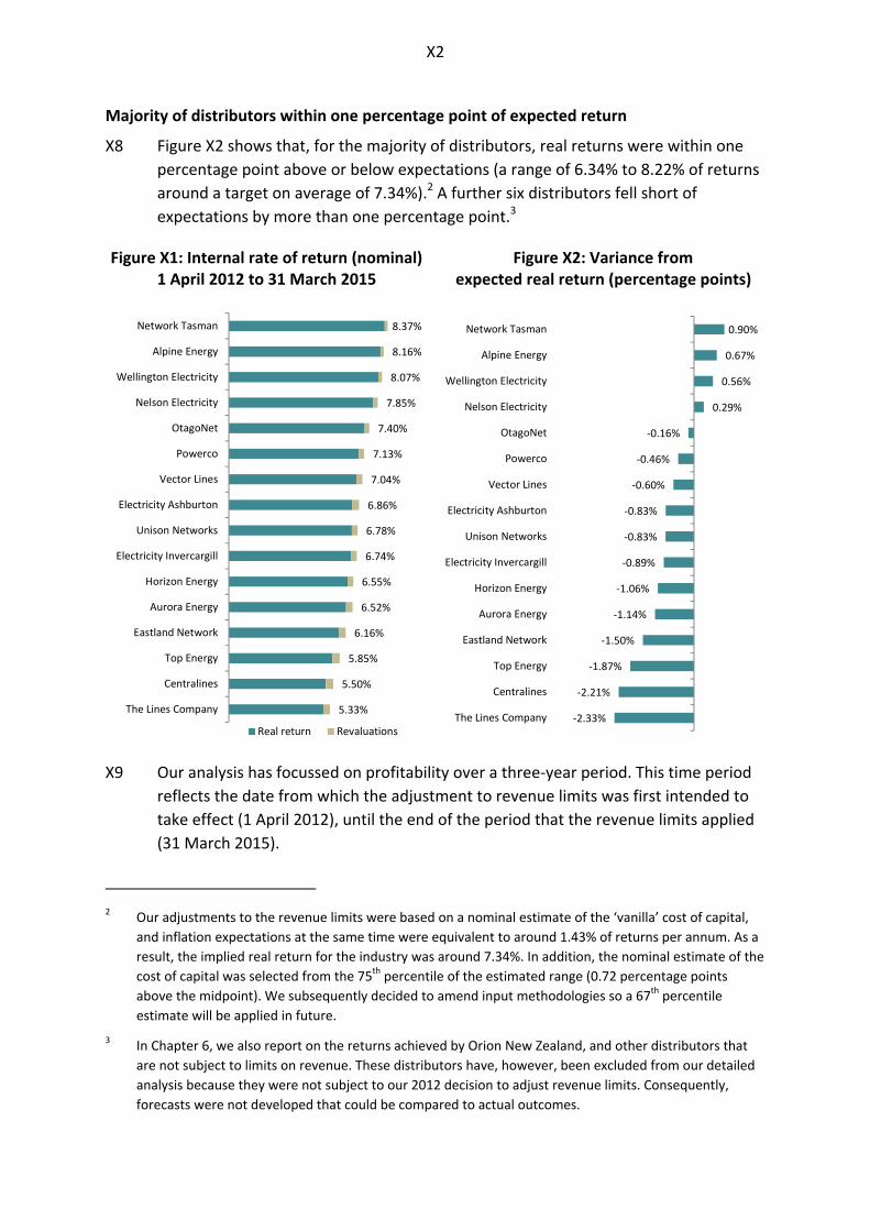
X8 Figure X2 shows that, for the majority of distributors, real returns were within one

percentage point above or below expectations (a range of 6.34% to 8.22% of returns

around a target on average of 7.34%).2 A further six distributors fell short of

expectations by more than one percentage point.3

Figure X1: Internal rate of return (nominal) 1 April 2012 to 31 March 2015

Figure X2: Variance from expected real return (percentage points)

X9 Our analysis has focussed on profitability over a three‐year period. This time period

reflects the date from which the adjustment to revenue limits was first intended to

take effect (1 April 2012), until the end of the period that the revenue limits applied

(31 March 2015).

2 Our adjustments to the revenue limits were based on a nominal estimate of the ‘vanilla’ cost of capital,

and inflation expectations at the same time were equivalent to around 1.43% of returns per annum. As a

result, the implied real return for the industry was around 7.34%. In addition, the nominal estimate of the

cost of capital was selected from the 75th percentile of the estimated range (0.72 percentage points

above the midpoint). We subsequently decided to amend input methodologies so a 67th percentile

estimate will be applied in future.

3 In Chapter 6, we also report on the returns achieved by Orion New Zealand, and other distributors that

are not subject to limits on revenue. These distributors have, however, been excluded from our detailed

analysis because they were not subject to our 2012 decision to adjust revenue limits. Consequently,

forecasts were not developed that could be compared to actual outcomes.

8.37%

8.16%

8.07%

7.85%

7.40%

7.13%

7.04%

6.86%

6.78%

6.74%

6.55%

6.52%

6.16%

5.85%

5.50%

5.33%

Network Tasman

Alpine Energy

Wellington Electricity

Nelson Electricity

OtagoNet

Powerco

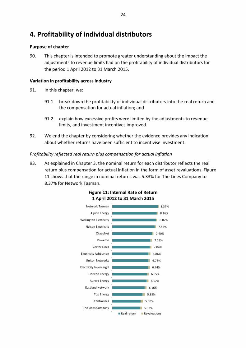
Vector Lines

Electricity Ashburton

Unison Networks

Electricity Invercargill

Horizon Energy

Aurora Energy

Eastland Network

Top Energy

Centralines

The Lines Company

Real return Revaluations

0.90%

0.67%

0.56%

0.29%

‐0.16%

‐0.46%

‐0.60%

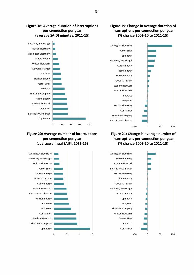
‐0.83%

‐0.83%

‐0.89%

‐1.06%

‐1.14%

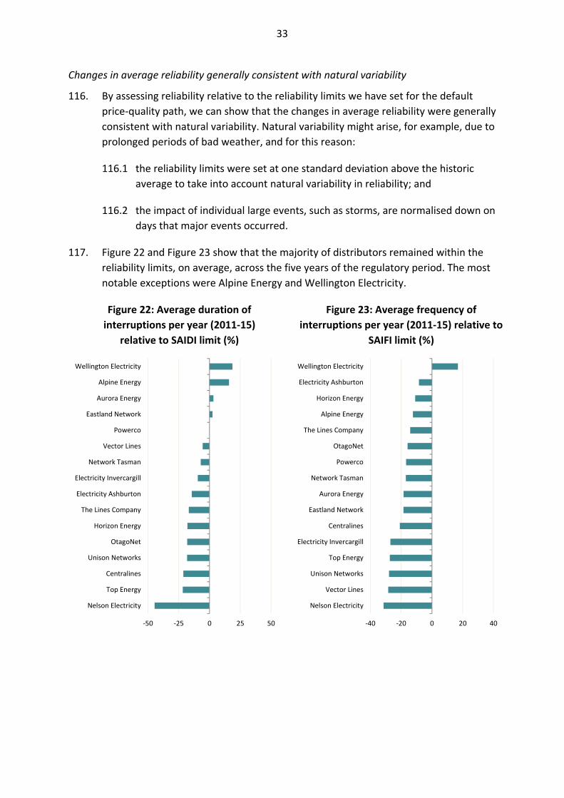
‐1.50%

‐1.87%

‐2.21%

‐2.33%

Network Tasman

Alpine Energy


Nelson Electricity

OtagoNet

Powerco

Vector Lines


Unison Networks


Horizon Energy

Aurora Energy

Eastland Network

Top Energy

Centralines

The Lines Company

X3

X10 The results indicate that excessive profits were limited by our adjustments to the

revenue limits. For example, had the revenue limits been left unadjusted,

Vector Lines would have recovered around $110m more profits than would have

been justified. The impacts on returns are shown in Figure X3.4

Figure X3: Impact of adjustments to revenue ($m)

Figure X4: Change in average capital expenditure relative to historic average (%)

X11 Figure X4 shows that investment increased relative to historic levels, which indicates

that the adjustments were consistent with distributors having continued incentives

to invest. The increases in capital expenditure were equivalent to around $97m of

additional investment over the three years (2015 prices).

X12 Trends therefore suggest that distributors had incentives to invest but, based on this

information alone, we are unable to reach conclusions about the quality of asset

management practices. Nor is it clear whether such spending reflects prudently

incurred costs.

4 All relevant distributors reported themselves as being compliant with the adjusted revenue limits.

‐150 ‐100 ‐50 0 50

Vector Lines

Eastland Network

Horizon Energy

Nelson Electricity


Aurora Energy

OtagoNet

Powerco


Centralines

Network Tasman


The Lines Company

Top Energy

Unison Networks

Alpine Energy

‐100 0 100 200 300 400

Nelson Electricity

Top Energy

Network Tasman

Eastland Network


Horizon Energy

Alpine Energy

OtagoNet

Powerco


Vector Lines

The Lines Company

Unison Networks


Aurora Energy

Centralines

X4

Breakdown of variance between actual and expected returns

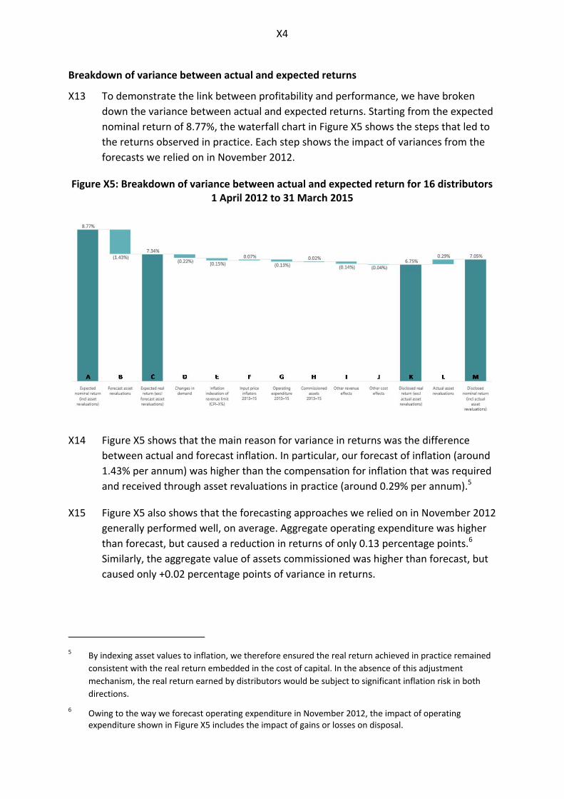
X13 To demonstrate the link between profitability and performance, we have broken

down the variance between actual and expected returns. Starting from the expected

nominal return of 8.77%, the waterfall chart in Figure X5 shows the steps that led to

the returns observed in practice. Each step shows the impact of variances from the

forecasts we relied on in November 2012.

Figure X5: Breakdown of variance between actual and expected return for 16 distributors 1 April 2012 to 31 March 2015

X14 Figure X5 shows that the main reason for variance in returns was the difference

between actual and forecast inflation. In particular, our forecast of inflation (around

1.43% per annum) was higher than the compensation for inflation that was required

and received through asset revaluations in practice (around 0.29% per annum).5

X15 Figure X5 also shows that the forecasting approaches we relied on in November 2012

generally performed well, on average. Aggregate operating expenditure was higher

than forecast, but caused a reduction in returns of only 0.13 percentage points.6

Similarly, the aggregate value of assets commissioned was higher than forecast, but

caused only +0.02 percentage points of variance in returns.

5 By indexing asset values to inflation, we therefore ensured the real return achieved in practice remained

consistent with the real return embedded in the cost of capital. In the absence of this adjustment

mechanism, the real return earned by distributors would be subject to significant inflation risk in both

directions.

6 Owing to the way we forecast operating expenditure in November 2012, the impact of operating expenditure shown in Figure X5 includes the impact of gains or losses on disposal.

X5

X16 The impact of each factor was, however, different for each distributor. Most notably,

where one percentage point is equivalent to around 14% of the target real return:

X16.1 differences between forecast and actual operating expenditure explained

between −1.72 and +0.67 percentage points of the variance in returns for

individual distributors; and

X16.2 differences between forecast and actual changes in demand explained

between −0.96 and +1.41 percentage points of the variance in returns for

individual distributors.

X17 For certain distributors, ‘other revenue effects’ explained a relatively significant

amount of the variance. For example, avoided cost of transmission payments

boosted returns by up to 0.75 percentage points. Pricing beneath the revenue limit

suppressed returns by a maximum of 1.74 percentage points.

X18 Similarly, a relatively significant amount of the variance for certain distributors was

explained by ‘other cost effects’. For example, differences from the forecast level of

net additions to the asset base prior to 1 April 2012 caused up to 2.20 percentage

points of variance in returns. And in some cases discretionary discounts and

consumer rebates boosted returns by up to 2.01 percentage points (by reducing tax

payable).

X19 Chapter 3 and Attachment A provide further information about the different sources

of variance, as well as quantifying the materiality of the effects for individual

distributors. We trust that this information will help you develop a greater

understanding of the performance of individual distributors.

Next steps

X20 Most immediately, our findings may be relevant to our first full review of input

methodologies under s 52Y of the Commerce Act. For example, the extent to which

distributors are exposed to volume risk is relevant to our decision on the form of

control.

X21 Our draft decisions on the input methodologies review are due on 16 June 2016.

2504924.17


1

2504924.17

1

2

3

4

56

7

89

10

11

612

13

14

15

16

17

18 19

2021

22

23

24

2526

27

26

28

29

1. Introduction

Purpose of report

1. This report is intended to improve stakeholder understanding about the impact that

the first periodic adjustment to revenue limits had on the profitability of

16 electricity distributors. We also provide information about the changes in network

reliability, and draw comparisons with other distributors.

Information disclosure regulation—our role under summary and analysis

2. As the economic regulator of 29 electricity distributors in New Zealand, we require

public disclosure of a range of information about performance. This information

includes asset management plans, pricing methodologies, and financial and network

data. The location of each distributor is shown in Figure 1.

Figure 1: Location of 29 electricity distributors

North Island

1. Top Energy

2. Northpower

3. Vector

4. Counties Power

5. WEL Networks

6. Powerco

7. Waipa Networks

8. The Lines Company

9. Unison

10. Horizon Energy

11. Eastland Networks

12. Centralines

13. Scanpower

14. Electra

15. Wellington

Electricity

South Island

16. Nelson Electricity

17. Buller Electricity

18. Network Tasman

19. Marlborough Lines

20. Westpower

21. Mainpower

22. Orion New Zealand

23. Electricity Ashburton

24. Alpine Energy

25. Network Waitaki

26. Aurora Energy

27. OtagoNet

28. The Power Company

29. Electricity Invercargill

3. The aim of information disclosure regulation is to allow people to assess whether the

purpose of Part 4 of the Commerce Act 1986 (the Act) is being met. In broad terms,

the 'Part 4 Purpose' is to promote the long‐term benefit of consumers, by promoting

outcomes consistent with those produced in competitive markets.7

7 The relevant outcomes are set out in (a)‐(d) of the Part 4 Purpose. Refer: s 52A(1) of the Act.

2

Improving stakeholder understanding through summary and analysis

4. Under s 53B of the Act, we are required to publish summary and analysis of the

information disclosed by distributors. The purpose of summary and analysis is to

promote greater understanding about the performance of distributors, their relative

performance, and changes in their performance over time.

5. To help improve stakeholder understanding, every year we consolidate the

quantitative information and publish the centralised database on our website.

We often receive positive feedback about these databases, including from the

distributors themselves.

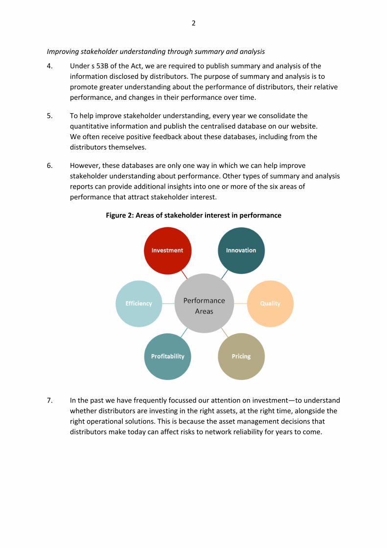
6. However, these databases are only one way in which we can help improve

stakeholder understanding about performance. Other types of summary and analysis

reports can provide additional insights into one or more of the six areas of

performance that attract stakeholder interest.

Figure 2: Areas of stakeholder interest in performance

7. In the past we have frequently focussed our attention on investment—to understand

whether distributors are investing in the right assets, at the right time, alongside the

right operational solutions. This is because the asset management decisions that

distributors make today can affect risks to network reliability for years to come.

3

8. Most recently, in 2013, our focus on investment continued with a summary and

analysis report that:8

8.1 highlighted wide variation in the expenditure plans disclosed by electricity

distributors; and

8.2 considered how the variation in the expenditure plans might be explained in

the context of underlying drivers.

9. We welcomed stakeholder engagement on this topic and expect to revisit this work

in future.

Focus for this report is on profitability

10. In this report we have chosen to focus on profitability, but we define profits

differently to most. Instead of looking to standard accounting definitions, we specify

regulatory rules for how costs are defined. This means we are able to keep a closer

eye on the profitability of the regulated services over time, even if the distributor is

part of a wider parent company.

11. Amongst other things, we hope this work will go some way towards answering

questions that are frequently asked of us about the profitability of distributors. Our

primary interest lies in understanding the extent to which profitability is comparable

to competitive markets, in which:

11.1 excessive profits are limited; and

11.2 appropriate investment incentives are in place.

12. While we are also interested in the pricing structures used to recover revenue, it is

the Electricity Authority that has primary responsibility for overseeing the practices

of distributors in this area. As a consequence, we have focussed on the revenue

recovered from prices overall, and the resulting level of profitability, rather than on

individual pricing structures.

8 Commerce Commission “Initial observations on forecasts disclosed by 29 electricity distributors in March

2013” (29 November 2013).

4

More specifically: the profitability of distributors that are subject to revenue limits

13. Although we will be reporting on the profitability of all distributors, our analysis

centres on the distributors that are subject to limits on revenue.9 In part, this is

because 'exempt' distributors have ownership arrangements in which profits are

returned directly to almost all consumers (in the form of rebates). Stakeholder

interest in profitability is therefore different for exempt distributors.

14. Our decision to reserve our more detailed analysis for the distributors subject to

revenue limits also has practical roots. Our approach to setting revenue limits

involved creating a forecasting model and we have used this model as the basis for

our more detailed analysis.

Variations in profitability expected—not a guaranteed rate of return

15. Our expectation is that profitability will vary under the revenue limits because

distributors are not guaranteed to earn any particular rate of return. Rather, returns

depend on the interplay, over a fixed duration, between the revenue limits that we

determine, and the costs and demand experienced by each distributor.

16. The advantage of setting revenue limits for a fixed duration (known as the

‘regulatory period’) is that it preserves, and potentially improves, the financial

incentive that each distributor has to improve its efficiency. This is because

distributors are rewarded with higher profits if they can control their expenditure.

17. Minimum standards for service quality are important too, because they mitigate the

risk that distributors will cut their costs by compromising quality. Distributors will

therefore be more likely to provide services at a quality that reflects consumer

demands.

9 As explained in Chapter 3, the limits on revenue are specified in the form of a weighted average price cap,

which means that distributors are able to earn higher revenues through increased volumes.

5

Understanding and improving the effectiveness of regulation

18. Amongst other things, by promoting greater understanding of the performance of

electricity distributors, we expect that summary and analysis will help us understand

and improve the effectiveness of regulation. The evidence base that we develop may

prove useful to a number of our workstreams.

19. For example, we are currently midway through a review of the up‐front rules,

requirements and processes of regulation, which are collectively referred to as ‘input

methodologies’. This is the first full review of input methodologies since they were

originally determined in December 2010.10

20. We will also have other opportunities to refine aspects of our regulatory settings

that are outside the scope of the input methodologies review. In particular, we can

make further improvements at the next reset of the revenue limits for electricity

distributors, or in our next suite of amendments to the disclosure requirements.

21. However, the current revenue limits, which expire on 31 March 2020, have already

been set and cannot be changed. The only provisions for reconsidering these

revenue limits relate to specific circumstances such as natural disasters or legislative

changes.

Our first comparison of supplier profitability based on original forecasts

22. The analysis presented in this report is the first time that we have undertaken

detailed profitability analysis of suppliers after a regulatory period. We welcome

feedback on our approach. We are particularly interested in feedback on our

calculation of internal rates of return and the comparisons to the expected return.

23. Feedback can be provided to us by email using the email address

[email protected], or during our process to review input

methodologies. This is not a formal submission process so there is no specific

deadline for feedback.

10 We are required to review each input methodology under s 52Y of the Commerce Act.

6

Data generally relied on ‘as disclosed’ by distributors

24. In this report, we have generally relied on data ‘as disclosed’ by distributors. We

have adopted this approach because we recognise that the onus is on distributors to

be sufficiently confident in their data before it is publicly disclosed. We also take

comfort from the fact that the information is subject to independent audit

requirements.

25. Nevertheless, some errors were still obvious in the information that had been

publicly disclosed, eg, the closing value in one year being different to the opening

value the following year. Where these issues were identified, we have corrected

these data points, in discussion with distributors.

26. However, without duplicating the efforts of distributors in ensuring their data is

robust, we recognise there is a risk of further errors being identified after this report

has been published. We therefore invite distributors to contact us if they identify an

error, and would like to request an opportunity to submit corrected data.

27. We note that the data disclosed by distributors is consistent with the rules and

requirements that we have set. Any changes to these in the future may result in

changes to our view of the distributors’ returns. Some potential changes would be

more material than others. For example, the rules for considering regulated party

transactions will be considered in the future, and could be more material than other

potential changes.

Material published alongside this report

28. We have published a range of supporting material for this report on our website,

including:

28.1 the data that we have used for our analysis;

28.2 the calculations and modelling used for our analysis; and

28.3 detailed analysis and findings for individual distributors.

29. In particular, we have reproduced charts that are equivalent to Figure 3, Figure A1,

and Figure A2 for each individual distributor that was subject to the 2012

adjustments to revenue limits.

7

2. First adjustment to revenue limits

Purpose of chapter

30. This chapter summarises the key features of our decision to adjust the revenue limits

for the first time in November 2012, which provides the context for our analysis of:

30.1 profitability over the period 1 April 2012 to 31 March 2015; and

30.2 quality of service over the period 1 April 2010 to 31 March 2015.

31. This chapter also explains why we have not analysed Orion New Zealand alongside

the other distributors that are subject to revenue limits.

First regulatory period under new Part 4—and a number of other regulatory ‘firsts’

32. The regulatory period 1 April 2010 to 31 March 2015 was the first under the new

Part 4 of the Commerce Act, and as such it is perhaps unsurprising that the time

period contained a number of other regulatory ‘firsts’. For the first time we:

32.1 adjusted revenue limits based on projected profitability; and

32.2 applied input methodologies to price setting.

33. Importantly, it was also the first regulatory period for a new type of regulation

known as ‘default/customised price‐quality regulation’. Under this type of

regulation, we set a default price‐quality path for each distributor, but individual

distributors could seek a customised price‐quality path instead.

34. The common feature between each type of ‘price‐quality path’ is that they specify

limits on revenue, and minimum quality standards. However, as explained in Box 1,

the two paths do differ in terms of how, and when, they are set. The ‘customised’

path is a more tailored alternative to the initial ‘default’ set for each distributor.

Box 1: Purpose of default/customised price‐quality regulation11

The purpose of default/customised price‐quality regulation is to provide a relatively low

cost way of setting price‐quality paths for electricity distributors, while allowing the

opportunity for individual distributors to have alternative price‐quality paths that better

meet their particular circumstances.

11 Refer: s 53K of the Act.

8

35. When we first set default price‐quality paths in November 2009, we recognised that

the revenue limits could be adjusted midway through the regulatory period, after

input methodologies had been determined for the first time. In particular,

adjustments could be made if materially different pricing outcomes were implied by

input methodologies.12

36. For that reason, in November 2009, we set the default price‐quality path for the first

regulatory period by simply rolling over the revenue limits that were already in place.

Quality standards reflected historic levels of performance. These default

price‐quality paths applied to all 17 distributors that were subject to price‐quality

regulation.

37. Then, in November 2012, we applied input methodologies to adjust the revenue

limits to better reflect the expected costs of each distributor. Input methodologies

affected our assessment of key cost components, such as the industry‐wide cost of

capital, and were applied alongside other assumptions (such as demand growth).

38. Taking our direction from the purpose of default/customised price‐quality

regulation, the other assumptions we relied on were developed in a relatively low

cost way. More costly approaches could be used to set a customised path, such as

those associated with audit, verification, and approval processes.

39. Consequently, in assessing profitability in November 2012, a variety of low cost

techniques were used. Forecasts of demand and expenditure were developed

through a combination of reliance on the supplier’s own forecasts, independent

forecasts, and simplifying assumptions.

40. Based on our low cost approaches, adjustments in both directions appeared

appropriate. For some distributors, reductions in the revenue limit were necessary to

limit excessive profits. For others, increases would preserve incentives to invest.

Consumers would benefit from different outcomes depending on the market.

41. Notably, because the revenue limits had not been adjusted since 2003, some of the

required increases were so significant that we had to smooth the increases over

multiple years to minimise price shocks to consumers. This is because, prior to the

adjustments, prices reflected information that was many years out of date.

12 Refer: s 54K(3) of the Act. This was a transitional provision that only applied to the first regulatory period.

9

Mid‐period reset focussed on profitability over a three‐year period

42. The analysis in this paper reflects the fact that the November 2012 reset occurred

midway through the regulatory period, and the focus of that reset was on returns

over a three‐year period (1 April 2012 to 31 March 2015).13 We have therefore

focussed on the level of profitability achieved during this period as it reflects the

date from which input methodologies were first intended to be reflected in pricing.

43. The aim of applying input methodologies over this period was to provide an

opportunity to earn an appropriate return in real terms, ie, after inflation.14

Focussing on real returns is common in overseas jurisdictions, as recognised by

Australasian expert Jeff Balchin (on behalf of Powerco Limited):15

the desirability of … protecting investors in long‐lived regulated assets from inflation risk

dates back to the 1970s, where the unexpectedly high rate of inflation in that decade and

beyond had a substantial adverse effect on the values of regulated businesses in the US, as

well as encouraging frequent applications for tariff resets. By the time that modern price cap

regulation emerged in the UK in the 1980s, inflation indexation of prices and underlying asset

values became a standard part of the regulatory regime.

For investors in regulated assets to be protected from inflation, regulated prices must be

determined such that the same real return (that is, the return above what is necessary to

compensate for the decline in the purchasing power of money) would be delivered, all else

constant, irrespective of the measured rate of inflation. This means that if inflation is higher

than forecast, then the nominal return (that is, the return that includes compensation for the

decline in the purchasing power of money) must also be correspondingly higher. I also

observe that the proposition that investors care about real rather than nominal returns is a

standard proposition in economics – it merely means that investors are sufficiently astute to

see through the influence of inflation on “headline” returns and assess the acceptability of

returns in terms of real purchasing power.

13 Although the changes to the revenue limits only came into effect on 1 April 2013, we applied claw back to

compensate distributors for the under or over recovery of revenue that occurred in the previous year.

This approach ensured that we achieved broadly similar outcomes for suppliers and consumers, in net

present value terms, as if the adjustment to revenue limits had been implemented in full on the date that

was originally envisaged (1 April 2012). For further reasoning, refer: Commerce Commission “Resetting

the 2010‐15 Default Price‐Quality Paths for 16 Electricity Distributors” (30 November 2012)

14 This aim is discussed further in the ‘RAB Indexation and Inflation Risk’ chapter of Dr Martin Lally, “Review

of further WACC issues” (22 May 2016).

15 PwC (for Powerco) “Draft Input Methodology for Default Price‐Quality Paths – Inflation Issues” (6 July

2012).

10

44. The importance of considering returns in real terms can be seen by looking at

changes over time in our nominal estimate of the cost of capital. For example:16

44.1 our estimate of the required nominal return from 1 April 2010 until 31 March

2015 was 8.77%, when forecast inflation implied a real return of 7.34% over

the period; and

44.2 our estimate of the required nominal return from 1 April 2012 until 31 March

2015 was 7.14%, when forecast inflation implied a real return of 6.32% over

the period.

45. For this reason, when adjusting the revenue limits, the forecast of inflation that we

relied on was the most recently available when the applicable nominal estimate of

the cost of capital was determined. We noted that “such an approach ensures that

the implied real return during the regulatory period is consistent with the inflation

expectations that are embedded in our estimate of the cost of capital”.17

…while quality standards remaining unchanged for the full five years…

46. As noted previously, although the revenue limits were adjusted midway through the

period, the quality standards remained unchanged. This is because the revenue

limits were adjusted to ensure input methodologies were reflected in pricing.

However, service quality is not one of the matters covered by input methodologies.

47. For this reason, the analysis of service quality that appears in this paper is based on

performance over the full five years of the regulatory period. The analysis of quality

of service therefore includes an additional two years of data than the analysis of

profitability.

…and Orion New Zealand were excluded following the Canterbury earthquakes

48. In light of the circumstances surrounding the Canterbury earthquakes, we excluded

Orion New Zealand from the scope of our November 2012 decision to minimise

consultation obligations on the business. We therefore did not develop forecasts in

the same way for Orion New Zealand as for other distributors.

16 All figures in this section correspond to the 75th percentile estimate of the ‘vanilla’ cost of capital. Given

the uncertainty of estimating the cost of capital, this uplift was intended to help mitigate the potential

asymmetric consequences on investment of estimation error. One of the practical effects of the uplift

was to provide compensation for catastrophic risk. We have since revised down the percentile that we

will rely on in future, from the 75th percentile to the 67th percentile.

17 Commerce Commission “Resetting the 2010‐15 Default Price‐Quality Paths for 16 electricity Distributors”

(30 November 2012); paragraph 4.19.

11

49. We recognised at the time that Orion New Zealand would apply for a customised

price‐quality path to better reflect its particular circumstances. Amongst other

things, the alternative price‐quality path that we set allowed Orion New Zealand to

recover increased expenditure associated with the network rebuild.18

50. For that reason, we have excluded Orion New Zealand from the more detailed

profitability analysis contained in this paper. However, we do expect to report in

more detail on the profitability of Orion New Zealand at a date closer to the end of

the customised price‐quality path.

18 More information on Orion’s customised price‐quality path is provided in: Commerce Commission

“Setting the customised price‐quality path for Orion New Zealand Limited” (29 November 2013).

12

3. Performance relative to expectations

Purpose of chapter

51. This chapter relies on our November 2012 forecasts to assess the main sources of

variance between actual and expected profitability for the period 1 April 2012 and

31 March 2015.

Breakdown of variance between actual and expected profitability

52. To demonstrate the link between profitability and performance, we have broken

down the sources of variance between actual and expected profitability. The

waterfall chart in Figure 3 shows the impact on returns of each difference between

actual outcomes varying from the assumptions we relied on in November 2012.

53. The starting point for the waterfall chart is the return we expected each distributor

to earn in nominal terms, based on a nominal estimate of the weighted average cost

of capital (WACC), and the end point is the return that was achieved by all

distributors in aggregate.19 Because it shows the effect at the industry level, Figure 3

is heavily influenced by larger distributors, such as Vector Lines, and Powerco

Limited.

54. In between the start and the end point of the waterfall is a sequence of steps, with

each step showing the impact on returns of a difference between our assumption

and the actual outcome. For example, there is a step that shows the impact on

returns of actual operating expenditure being different from forecast.

55. The first and last steps in the waterfall are different from the steps in between,

because they both relate to the portion of returns that is attributable to inflation

indexation of asset values.20 By contrast, the intervening steps relate to the ‘real

returns’ that arise as a result of net revenue recovered during the three‐year period.

19 As noted in Chapter 2, the expected return reflected the 75th percentile estimate of the industry wide

cost of capital. The use of this percentile represented an uplift of 0.72 percentage points relative to the

midpoint.

20 Revaluations increase supplier returns by increasing the return on and of capital that is expected in future

and vice versa.

13

2504924.17

Figure 3: Industry variance from pricing assumptions for period 1 April 2013 to 31 March 2015

14

2504924.17

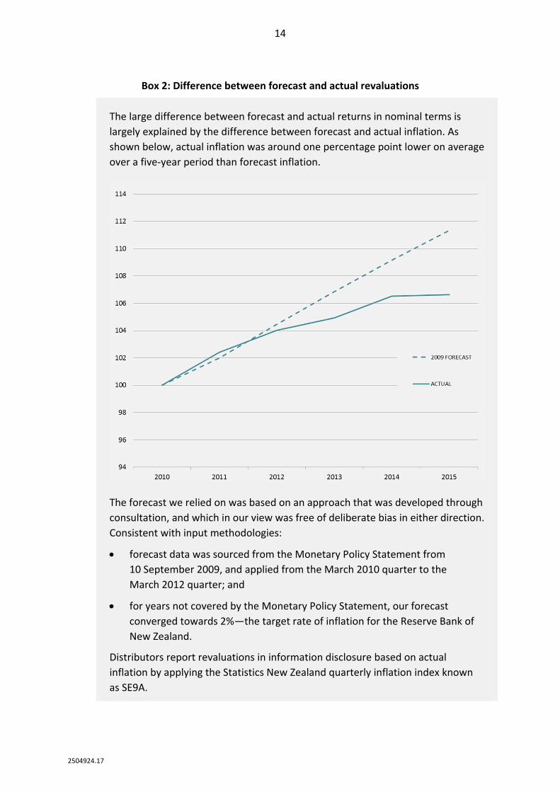
Box 2: Difference between forecast and actual revaluations

The large difference between forecast and actual returns in nominal terms is

largely explained by the difference between forecast and actual inflation. As

shown below, actual inflation was around one percentage point lower on average

over a five‐year period than forecast inflation.

The forecast we relied on was based on an approach that was developed through

consultation, and which in our view was free of deliberate bias in either direction.

Consistent with input methodologies:

forecast data was sourced from the Monetary Policy Statement from

10 September 2009, and applied from the March 2010 quarter to the

March 2012 quarter; and

for years not covered by the Monetary Policy Statement, our forecast

converged towards 2%—the target rate of inflation for the Reserve Bank of

New Zealand.

Distributors report revaluations in information disclosure based on actual

inflation by applying the Statistics New Zealand quarterly inflation index known

as SE9A.

15

‘Nominal return’ reflected performance‐related real return and compensation for inflation

56. Figure 3 also shows that the nominal return for the industry reflected the real return

of 6.75% plus compensation for actual inflation in the form of asset revaluations.21

Inflation indexation of asset values added around 0.29% to industry returns.22

57. Although inflation was lower than forecast, the practical effect of indexing asset

values to actual inflation was to ensure that the real return was consistent with the

real return embedded in the cost of capital. In the absence of this adjustment

mechanism, the real return earned by distributors would be subject to inflation risk

in both directions.

58. A benefit of applying inflation indexation to asset values is therefore that real returns

are more stable over time, which in our view is more conducive to a regulatory

environment that supports long‐term network investment. However, we are open to

receiving views on whether we should change this approach as part of our review of

input methodologies.

‘Real return’ for industry of 6.75% below target real return of 7.34%

59. By comparing Steps C and K in Figure 3, both of which exclude the effects of asset

revaluations on returns, we can see that the actual real return for the industry of

6.75% was below the target real return of 7.34%.23 The returns for individual

distributors are shown in Chapter 4.

60. Figure 3 indicates that at the industry level our models for forecasting expenditure

and revenue growth performed reasonably well. Although some factors affected

individual distributors more than others, there were no sources of variance for the

industry as a whole that were equivalent to more than 0.3 percentage points of

returns.

21 For presentational purposes we have defined the real return as being equal to the nominal return less the

impact of asset revaluations. In practice, the relationship between the real return and the nominal return

is more complicated. For example, the relationship between the real return, inflation, and the nominal

return is multiplicative rather than additive.

22 The definition of inflation that we apply when revaluing regulated assets excludes the impact of changes in Goods and Services Tax (GST). This is because individuals and entities that are GST registered (such as electricity distributors) face the same price for goods and services before and after the tax change.

23 The actual real return for the industry was, however, above the real return implied by the midpoint

estimate of the cost of capital of around 6.62%, ie, 7.34% less the uplift of 0.72 percentage points from

the midpoint of the estimated range.

16

2504924.17

Impact of changes in demand

61. Step D in Figure 3 shows the variance in returns caused by differences between the

actual and expected impact of changes in demand. It is the impact on revenue

growth that would have occurred as a result of changes in demand even if average

prices remained unchanged (which we have referred to in the past as ‘constant price

revenue growth’).

62. This variance arises because the limit on revenue is specified in the form of a ‘price

cap’, which means that distributors are exposed to revenue risk with respect to

changes in demand.24 Specifically, an increase in quantities boosts revenue, and a fall

in quantities reduces revenue.

63. Distributors differ in terms of the quantities upon which their prices are based. The

majority of distributors recover revenue through a combination of fixed charges for

connections, and variable charges for throughput. Other distributors recover

revenue through capacity based charges.

64. The pricing approach applied by a distributor will affect the extent to which revenues

are exposed to demand risk. For example, Wellington Electricity recently changed to

have a greater proportion of fixed charges, which means changes in throughput have

less of an impact than with a larger proportion of variable charges. However,

Wellington Electricity remains exposed to variations in the number of connections.

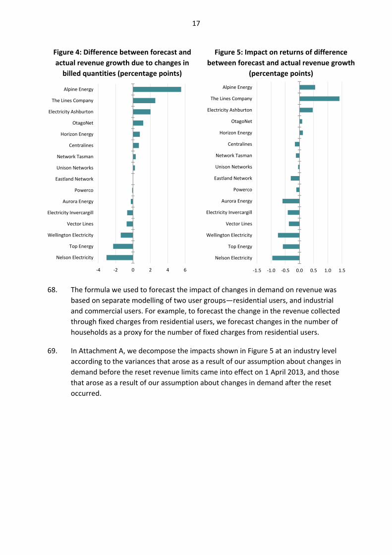
65. Figure 5 shows that the variation in returns attributable to changes in demand

relative to forecast were −1.0 to +1.4 percentage points. The net effect for the

industry as a whole was –0.22 percentage points, but only five distributors saw an

increase in returns relative to our expectations.

66. These impacts reflect differences between our forecast of the impact of changes in

billed quantities, and the actual impact of changes in billed quantities. As shown in

Figure 4, the largest difference was 5.5 percentage points of revenue growth per

year for Alpine Energy following a period of sustained increases in industrial demand.

67. The relative ranking of a distributor in terms of variation in the growth rate for

demand (Figure 4) does not always map across to the same relative ranking in terms

of variation in returns (Figure 5). This is because the growth rate is calculated as an

average over three years, but in practice differences in the earlier years will have a

greater impact on returns than differences in later years.25

24 As part of the review of input methodologies, we are required to consider whether a price cap

remains the most appropriate form of control for electricity distributors.

25 In the case of Unison, Centralines, and Network Tasman, the profile of growth explains why average

demand growth above forecast resulted in a negative impact on returns.

17

Figure 4: Difference between forecast and

actual revenue growth due to changes in

billed quantities (percentage points)

Figure 5: Impact on returns of difference

between forecast and actual revenue growth

(percentage points)

68. The formula we used to forecast the impact of changes in demand on revenue was

based on separate modelling of two user groups—residential users, and industrial

and commercial users. For example, to forecast the change in the revenue collected

through fixed charges from residential users, we forecast changes in the number of

households as a proxy for the number of fixed charges from residential users.

69. In Attachment A, we decompose the impacts shown in Figure 5 at an industry level

according to the variances that arose as a result of our assumption about changes in

demand before the reset revenue limits came into effect on 1 April 2013, and those

that arose as a result of our assumption about changes in demand after the reset

occurred.

‐4 ‐2 0 2 4 6

Alpine Energy

The Lines Company


OtagoNet

Horizon Energy

Centralines

Network Tasman

Unison Networks

Eastland Network

Powerco

Aurora Energy


Vector Lines


Top Energy

Nelson Electricity

‐1.5 ‐1.0 ‐0.5 0.0 0.5 1.0 1.5

Alpine Energy

The Lines Company


OtagoNet

Horizon Energy

Centralines

Network Tasman

Unison Networks

Eastland Network

Powerco

Aurora Energy


Vector Lines


Top Energy

Nelson Electricity

18

Inflation indexation of revenue limit (CPI‐X%) and input price inflators

70. Indexation of the revenue limit to inflation is intended to ensure that revenues are

updated annually during the period in a way that mimics economy wide pressures on

profitability, in light of changes in input prices. In our view, therefore, the variance

for inflation indexation of the revenue limit should be considered alongside the

variance for the input price inflators used to predict expenditure.

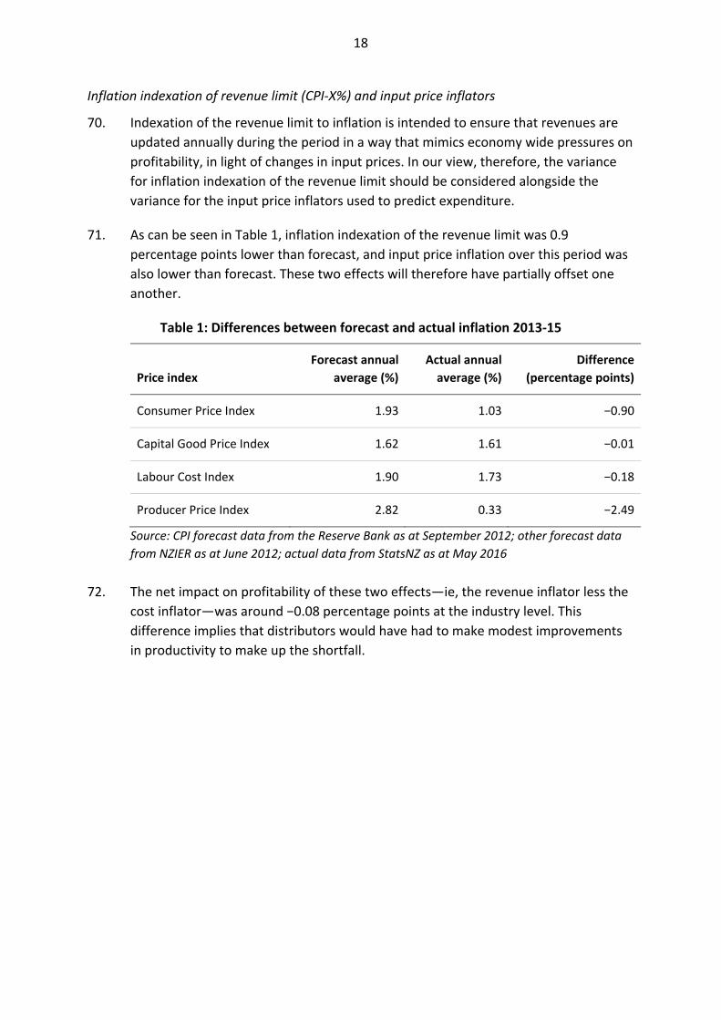
71. As can be seen in Table 1, inflation indexation of the revenue limit was 0.9

percentage points lower than forecast, and input price inflation over this period was

also lower than forecast. These two effects will therefore have partially offset one

another.

Table 1: Differences between forecast and actual inflation 2013‐15

Price index

Forecast annual

average (%)

Actual annual

average (%)

Difference

(percentage points)

Consumer Price Index 1.93 1.03 −0.90

Capital Good Price Index 1.62 1.61 −0.01

Labour Cost Index 1.90 1.73 −0.18

Producer Price Index 2.82 0.33 −2.49

Source: CPI forecast data from the Reserve Bank as at September 2012; other forecast data

from NZIER as at June 2012; actual data from StatsNZ as at May 2016

72. The net impact on profitability of these two effects—ie, the revenue inflator less the

cost inflator—was around −0.08 percentage points at the industry level. This

difference implies that distributors would have had to make modest improvements

in productivity to make up the shortfall.

19

Capital and operating expenditure after 1 April 2013 in constant prices

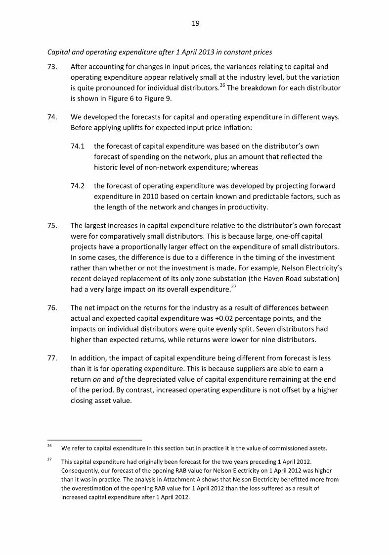
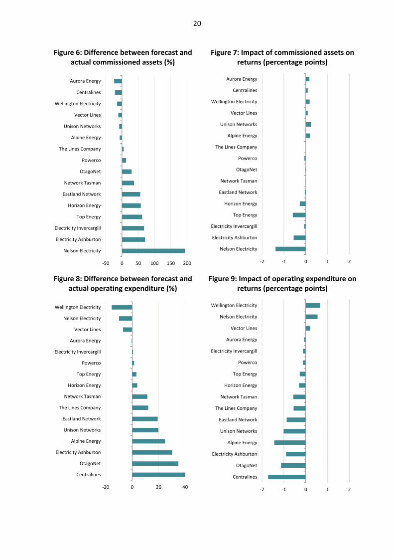
73. After accounting for changes in input prices, the variances relating to capital and

operating expenditure appear relatively small at the industry level, but the variation

is quite pronounced for individual distributors.26 The breakdown for each distributor

is shown in Figure 6 to Figure 9.

74. We developed the forecasts for capital and operating expenditure in different ways.

Before applying uplifts for expected input price inflation:

74.1 the forecast of capital expenditure was based on the distributor’s own

forecast of spending on the network, plus an amount that reflected the

historic level of non‐network expenditure; whereas

74.2 the forecast of operating expenditure was developed by projecting forward

expenditure in 2010 based on certain known and predictable factors, such as

the length of the network and changes in productivity.

75. The largest increases in capital expenditure relative to the distributor’s own forecast

were for comparatively small distributors. This is because large, one‐off capital

projects have a proportionally larger effect on the expenditure of small distributors.

In some cases, the difference is due to a difference in the timing of the investment

rather than whether or not the investment is made. For example, Nelson Electricity’s

recent delayed replacement of its only zone substation (the Haven Road substation)

had a very large impact on its overall expenditure.27

76. The net impact on the returns for the industry as a result of differences between

actual and expected capital expenditure was +0.02 percentage points, and the

impacts on individual distributors were quite evenly split. Seven distributors had

higher than expected returns, while returns were lower for nine distributors.

77. In addition, the impact of capital expenditure being different from forecast is less

than it is for operating expenditure. This is because suppliers are able to earn a

return on and of the depreciated value of capital expenditure remaining at the end

of the period. By contrast, increased operating expenditure is not offset by a higher

closing asset value.

26 We refer to capital expenditure in this section but in practice it is the value of commissioned assets.

27 This capital expenditure had originally been forecast for the two years preceding 1 April 2012.

Consequently, our forecast of the opening RAB value for Nelson Electricity on 1 April 2012 was higher

than it was in practice. The analysis in Attachment A shows that Nelson Electricity benefitted more from

the overestimation of the opening RAB value for 1 April 2012 than the loss suffered as a result of

increased capital expenditure after 1 April 2012.

20

Figure 6: Difference between forecast and actual commissioned assets (%)

Figure 7: Impact of commissioned assets on returns (percentage points)

Figure 8: Difference between forecast and actual operating expenditure (%)

Figure 9: Impact of operating expenditure on returns (percentage points)

‐50 0 50 100 150 200

Aurora Energy

Centralines


Vector Lines

Unison Networks

Alpine Energy

The Lines Company

Powerco

OtagoNet

Network Tasman

Eastland Network

Horizon Energy

Top Energy



Nelson Electricity

‐2 ‐1 0 1 2

Nelson Electricity



Top Energy

Horizon Energy

Eastland Network

Network Tasman

OtagoNet

Powerco

The Lines Company

Alpine Energy

Unison Networks

Vector Lines


Centralines

Aurora Energy

‐20 0 20 40


Nelson Electricity

Vector Lines

Aurora Energy


Powerco

Top Energy

Horizon Energy

Network Tasman

The Lines Company

Eastland Network

Unison Networks

Alpine Energy


OtagoNet

Centralines

‐2 ‐1 0 1 2


Nelson Electricity

Vector Lines

Aurora Energy


Powerco

Top Energy

Horizon Energy

Network Tasman

The Lines Company

Eastland Network

Unison Networks

Alpine Energy


OtagoNet

Centralines

21

78. The net effect on returns of the differences between actual and expected operating

expenditure at the industry level was −0.13 percentage points.28 The majority of

distributors spent more operating expenditure than was forecast, while only four

spent less.

79. We have also looked at whether the variances in operating expenditure could have

been associated with, and offset by, the impact of changes in demand. Figure 10

shows that, for some of the distributors, the impact of the variance in demand was

offset, at least in part, by the impact of the variance in operating expenditure.

However, the offsetting effect does not occur for all distributors.

Figure 10: Comparison of variances caused by operating expenditure versus the impact of demand growth on revenue (percentage points)

28 Owing to the way we forecast operating expenditure in November 2012, the impact of operating

expenditure shown in Figure 8 and Figure 9 includes the impact of gains or losses on disposal.

‐2

‐1

0

1

2

‐2 ‐1 0 1 2

Impact on returns of difference between actual

and forecast demand

Impact on returns of operating expenditure 2013‐15

22

80. What Figure 10 does not tell us, however, is whether the variance in operating

expenditure was:

80.1 caused by the same demand effect that resulted in a change in revenue, eg, increased connections would be associated with higher operating costs as well as higher fixed charges; or

80.2 a decision by the distributor to reduce operating expenditure in order to maintain returns in response to lower than forecast demand.

81. In future, we may consider in more detail the extent to which changes in operating

expenditure can be explained by drivers such as weather patterns or changes in

demand. Amongst other things, analysis of this nature may help stakeholders

understand whether expenditure is efficient.

82. At this stage, however, we are cautious about reaching conclusions about the

efficiency of expenditure based on the information available. For example, additional

expenditure may be required to maintain a level of quality that is sufficiently valued

by consumers, in response to events occurring during the period.

23

Other revenue effects

83. Attachment A provides a breakdown of the −0.14 percentage points of variance in

returns that is attributable to ‘other revenue effects’. These include:

83.1 impacts that broadly offset one another (such as the impact of the delay to

the reset, and the impact of associated claw‐back amounts); and

83.2 impacts that do not offset one another, such as pricing beneath the revenue

limit and differences between actual and forecast other regulatory income.

84. At the aggregate level the most material of the second group was pricing beneath

the limit, which resulted in returns being 0.14 percentage points lower than

expected. Variance in other factors was relatively limited at the aggregate level. In

particular:

84.1 other regulatory income (excluding gains and losses on disposals), accounted for +0.01 percentage points of variance in returns; and

84.2 avoided cost of transmission payments accounted for +0.03 percentage points of variance in returns.

85. However, individual distributors are affected more than others. For example, the

maximum variance in returns was caused by differences from forecast:

85.1 avoided costs of transmission payments (+0.75 percentage points); and

85.2 pricing beneath the revenue limit (−1.74 percentage points).

86. Attachment A provides further information about ‘other revenue effects’.

Other cost effects

87. Attachment A also breaks down the −0.04 percentage points of variance in returns

that is attributable to ‘other cost effects’. Notably, although the aggregate impact

was quite small, ‘other cost effects’ explained a significant amount of the variance

between actual and expected returns for some distributors.

88. For example, the maximum variance in returns was caused by differences from

forecast:

88.1 capital expenditure prior to 1 April 2012 (+2.20 percentage points); and

88.2 discretionary discounts and consumer rebates (2.01 percentage points).

89. Attachment A provides further information on ‘other cost effects’.

24

4. Profitability of individual distributors

Purpose of chapter

90. This chapter is intended to promote greater understanding about the impact the

adjustments to revenue limits had on the profitability of individual distributors for

the period 1 April 2012 to 31 March 2015.

Variation in profitability across industry

91. In this chapter, we:

91.1 break down the profitability of individual distributors into the real return and the compensation for actual inflation; and

91.2 explain how excessive profits were limited by the adjustments to revenue limits, and investment incentives improved.

92. We end the chapter by considering whether the evidence provides any indication

about whether returns have been sufficient to incentivise investment.

Profitability reflected real return plus compensation for actual inflation

93. As explained in Chapter 3, the nominal return for each distributor reflects the real

return plus compensation for actual inflation in the form of asset revaluations. Figure

11 shows that the range in nominal returns was 5.33% for The Lines Company to

8.37% for Network Tasman.

Figure 11: Internal Rate of Return 1 April 2012 to 31 March 2015

8.37%

8.16%

8.07%

7.85%

7.40%

7.13%

7.04%

6.86%

6.78%

6.74%

6.55%

6.52%

6.16%

5.85%

5.50%

5.33%

Network Tasman

Alpine Energy


Nelson Electricity

OtagoNet

Powerco

Vector Lines


Unison Networks


Horizon Energy

Aurora Energy

Eastland Network

Top Energy

Centralines

The Lines Company

Real return Revaluations

25

94. Figure 11 also shows that the impact of inflation indexation of asset values on

returns varied slightly across each distributor. In particular, the size of the effect of

asset revaluations ranged from 0.16 percentage points to 0.40 percentage points.

This variation is primarily due to the size and timing of each distributor’s capital

expenditure relative to its asset value.29

95. Figure 12 separates out the real return component and Figure 13 compares the real

return to that embedded in our nominal estimate of the cost of capital, ie, after

deducting the impact of the forecast of asset revaluations.

Figure 12: Real returns 1 April 2012 to 31 March 2015

Figure 13: Variation from expected real return (percentage points)

96. Figure 13 shows that, for the majority of distributors, real returns were within one

percentage point above or below our expectations when the revenue limits were

adjusted.30 A further six distributors fell short of expectations by more than one

percentage point.

29 The size and timing of capital expenditure affects the level of revaluations occurring during the period.

Because the real return is the residual between the nominal return and asset revaluations, some degree of variation in real returns across distributors is inevitable.

30 Our adjustments to the revenue limits were based on a nominal estimate of the cost of capital, and

inflation expectations at the same time were equivalent to around 1.43% of returns per annum, so the

real return for the industry was expected to be around 7.34%. In addition, the nominal estimate of the

cost of capital was selected from the 75th percentile of the estimated range, and was 0.72 percentage

points above the midpoint. Therefore, the real return implied by the midpoint was 6.62%.

8.22%

7.99%

7.88%

7.61%

7.16%

6.86%

6.72%

6.49%

6.49%

6.43%

6.26%

6.18%

5.82%

5.45%

5.11%

4.99%

Network Tasman

Alpine Energy


Nelson Electricity

OtagoNet

Powerco

Vector Lines


Unison Networks


Horizon Energy

Aurora Energy

Eastland Network

Top Energy

Centralines

The Lines Company

0.90%

0.67%

0.56%

0.29%

‐0.16%

‐0.46%

‐0.60%

‐0.83%

‐0.83%

‐0.89%

‐1.06%

‐1.14%

‐1.50%

‐1.87%

‐2.21%

‐2.33%

Network Tasman

Alpine Energy


Nelson Electricity

OtagoNet

Powerco

Vector Lines


Unison Networks


Horizon Energy

Aurora Energy

Eastland Network

Top Energy

Centralines

The Lines Company

26

97. Of the six distributors with profitability significantly below expectations, the

variances were primarily explained as follows:

97.1 The Lines Company—pricing beneath the limit and operating expenditure (−1.74 and −0.55 percentage points respectively);

97.2 Centralines—higher than forecast operating expenditure (−1.72 percentage points);

97.3 Top Energy—pricing beneath the limit and capital expenditure (−1.13 and −0.59 percentage points respectively);

97.4 Eastland—higher than forecast operating expenditure and lower than forecast billed quantities (−0.87 and −0.41 percentage points respectively);

97.5 Aurora Energy—lower than forecast billed quantities and other cost effects (−0.81 and −0.83 percentage points respectively); and

97.6 Horizon Energy—higher than forecast operating expenditure, capital expenditure, and other cost effects (−0.31, −0.27, and −0.86 respectively).

Excessive profits limited by reset and investment incentives improved

98. As shown in Figure 15, had the revenue limits not been reset, Vector Lines would

have recovered around $110m more in profits than would have been justified.

Indeed, the delay to the reset resulted in Vector Lines maintaining prices above costs

for an additional one year out of three. However, when resetting the revenue limits

in the second of the three years, claw‐back was applied to neutralise the impact of

the delay.

99. At the other end of the profitability distribution were a number of distributors that

were forecast to recover insufficient revenue. As explained in Chapter 2, this is

because the original revenue limits were a number of years out of date. Increases in

the revenue limits were therefore appropriate to preserve incentives to invest.

27

Figure 14: Impact of adjustments to revenue ($m)31

Figure 15: Impact of adjustments to revenue limits on returns (percentage

points)

Returns appear sufficient to incentivise investment

100. One indicator that returns were sufficient to incentivise investment is the general

increase in expenditure that has been observed recently relative to historic levels.

These trends therefore suggest that distributors had sufficient incentives to invest

more than historic levels.

101. However, based on this information alone, we are unable to reach conclusions about

the quality of asset management practices. Nor is it clear whether such spending

reflects prudently incurred costs, although distributors did have incentives to keep

costs under control. This is because any increases in expenditure would have

resulted in returns lower than they would have been otherwise.

31 All relevant distributors reported themselves as being compliant with the adjusted revenue limits.

‐150 ‐100 ‐50 0 50

Vector Lines

Eastland Network

Horizon Energy

Nelson Electricity


Aurora Energy

OtagoNet

Powerco


Centralines

Network Tasman


The Lines Company

Top Energy

Unison Networks

Alpine Energy

‐2 ‐1 0 1 2 3 4 5 6

Vector Lines

Eastland Network

Horizon Energy

Nelson Electricity


Aurora Energy

OtagoNet

Powerco


Centralines

Network Tasman


The Lines Company

Top Energy

Unison Networks

Alpine Energy

28

Change in average expenditure relative to historic average (2015 prices)

Figure 16: Capital expenditure (%) Figure 17: Operating expenditure (%)32

102. Figure 16 and Figure 17 indicate that the annual average level of capital and

operating expenditure was higher than historic levels for the period 1 April 2012 to

31 March 2015. For five out of 16 distributors, investment was between 0% and 20%

higher than historic averages, and for eight distributors, investment increased by

significantly more than 20%.

32 Includes pass through costs and recoverable costs.

‐100 0 100 200 300 400

Nelson Electricity

Top Energy

Network Tasman

Eastland Network


Horizon Energy

Alpine Energy

OtagoNet

Powerco


Vector Lines

The Lines Company

Unison Networks


Aurora Energy

Centralines

‐20 0 20 40

The Lines Company

OtagoNet

Centralines


Eastland Network

Alpine Energy

Unison Networks

Vector Lines

Aurora Energy

Network Tasman

Nelson Electricity


Powerco

Horizon Energy

Top Energy


29

5. Changes in network reliability

Purpose of chapter

103. Although our primary focus in this report is profitability, this chapter analyses the

changes in network reliability that occurred during the first regulatory period to

provide a more rounded picture of performance.

Network reliability is the main measure of quality of service

104. At present, the average number and duration of interruptions experienced by

consumers is the main way we measure quality of service. A recent working group of

the Electricity Networks Association (ENA) summarised customer surveys,

undertaken by distributors, and found the frequency and duration of power cuts to

be the most important aspect of quality for consumers.

105. However, as noted in Box 3, changes in network reliability do not necessarily reflect

changes in the risk of future asset failure. We must therefore be cautious about

reaching conclusions about the current level of service being provided to consumers

based purely on the level of reliability currently being experienced on the network.

106. In practice, the impact of poor asset management practices on network reliability

may only be evident in the event of a significant and sudden asset failure, or through

a steady deterioration in reliability over a number of years. For this reason, we have

started to require that distributors disclose additional information about the impact

of investments on the network (such as the health and condition of assets).

107. Despite the limitations, we think that information about reliability provides

additional context for understanding the profitability of distributors. We have,

however, deliberately stopped short of drawing direct comparisons between

distributor profitability and changes in reliability. Rather the information is provided

to help identify where further investigation to improve understanding may be

required.

108. Variation in the average level of reliability experienced by consumers, and a

comparison with historic performance, is shown in Figure 18 to Figure 21. In the

sections that follow, we:

108.1 identify and explain the reasons for wide variation between distributors in the average number and duration of interruptions; and

108.2 examine in more detail the changes in reliability over time, relative to natural

levels of variability.

109. We then provide additional information about the most significant deteriorations in

reliability that occurred between 1 April 2010 and 31 March 2015.

30

Box 3: Measures of reliability

Two internationally recognised measures of reliability shown in Figure 18 to Figure

21 are:

System Average Interruption Duration Index (SAIDI); and

System Average Interruption Frequency Index (SAIFI).

The benefit of relying on these measures is that they measure reliability in

aggregate across all consumers for each distributor. Therefore, the measures

provide a simple, cost‐effective, and transparent method of understanding

changes in performance over time.

These measures do, however, have obvious limitations. For example:

the level of reliability experienced by individuals, groups, or classes of

consumers may be very different from average reliability;

the extent to which consumers are notified in advance will affect the costs

imposed by an interruption;

the reliability of the low voltage parts of the networks (ie, less than 3.3 kV) are

not taken into account; and

the average level of network reliability may not accurately reflect the risks

associated with past and present asset management practices.

In addition, other factors—such as communication during a power outage—will also

affect the overall quality of service experienced by consumers. Consequently, we

recognise that this area of performance would merit further analysis in its own right,

potentially alongside or in support of industry‐led initiatives.

31

Figure 18: Average duration of interruptions per connection per year

(average SAIDI minutes, 2011‐15)

Figure 19: Change in average duration of interruptions per connection per year

(% change 2003‐10 to 2011‐15)

Figure 20: Average number of interruptions per connection per year

(average annual SAIFI, 2011‐15)

Figure 21: Change in average number of interruptions per connection per year

(% change 2003‐10 to 2011‐15)

0 200 400 600 800


Nelson Electricity


Aurora Energy

Unison Networks

Network Tasman

Centralines

Horizon Energy

Vector Lines

Powerco

The Lines Company

Alpine Energy

Eastland Network

OtagoNet


Top Energy

‐50 0 50 100


Vector Lines

Top Energy


Aurora Energy

Alpine Energy

Horizon Energy

Network Tasman

Eastland Network

Unison Networks

Powerco

OtagoNet

Nelson Electricity

Centralines

The Lines Company


0 2 4 6



Nelson Electricity

Vector Lines

Aurora Energy

Network Tasman

Alpine Energy

Unison Networks


Horizon Energy

Powerco

OtagoNet

Centralines

Eastland Network

The Lines Company

Top Energy

‐50 0 50 100


Horizon Energy

Eastland Network


Nelson Electricity

Alpine Energy

Network Tasman


Aurora Energy

Top Energy

OtagoNet

The Lines Company

Unison Networks

Vector Lines

Powerco

Centralines

32

Variation in average duration and frequency of interruptions

111. Figure 18 and Figure 20 show that between 1 April 2010 and 31 March 2015:

111.1 the average duration of interruptions varied between 41 and 722 minutes per

connection per year; and

111.2 the average number of interruptions varied between 0.7 and 5.6

interruptions per connection per year.

112. This variation is likely to be explained, at least in part, by differences in the

characteristics of each network. Commonly cited characteristics include the

following:

112.1 Network design or topology—the type and configuration of asset used to

supply consumers is impacted by historic design decisions, eg, voltage levels

and extent of undergrounding of the network;

112.2 Network topography—the terrain of the network can affect the cost of

accessing assets; and

112.3 Composition of consumer connections—different types of consumers have

different needs, which may affect the cost of serving these consumers.

113. In addition, the existing reliability of each network may reflect regional differences in

consumer preferences, given the link between the cost and quality of a service. For

example, industrial and commercial centres may place greater emphasis on

reliability, whereas affordability may be more important in other areas.

Reliability of price‐quality regulated distributors generally similar to past

114. Figure 19 and Figure 21 show that, with the exception of Wellington Electricity:

114.1 the average duration of interruptions varied between 35% above and 23% below historic levels; and

114.2 the average number of interruptions varied between 15% above and 26%

below historic levels.

115. These changes over time will to some extent reflect natural variability due to

changes in environmental factors. This is because the information in Figure 18 to

Figure 21 has not been adjusted for events such as storms. Rather, the figures are

intended to reflect the actual level of reliability experienced by consumers.

33

Changes in average reliability generally consistent with natural variability

116. By assessing reliability relative to the reliability limits we have set for the default

price‐quality path, we can show that the changes in average reliability were generally

consistent with natural variability. Natural variability might arise, for example, due to

prolonged periods of bad weather, and for this reason:

116.1 the reliability limits were set at one standard deviation above the historic

average to take into account natural variability in reliability; and

116.2 the impact of individual large events, such as storms, are normalised down on

days that major events occurred.

117. Figure 22 and Figure 23 show that the majority of distributors remained within the

reliability limits, on average, across the five years of the regulatory period. The most

notable exceptions were Alpine Energy and Wellington Electricity.

Figure 22: Average duration of

interruptions per year (2011‐15)

relative to SAIDI limit (%)

Figure 23: Average frequency of

interruptions per year (2011‐15) relative to

SAIFI limit (%)

‐50 ‐25 0 25 50


Alpine Energy

Aurora Energy

Eastland Network

Powerco

Vector Lines

Network Tasman



The Lines Company

Horizon Energy

OtagoNet

Unison Networks

Centralines

Top Energy

Nelson Electricity

‐40 ‐20 0 20 40



Horizon Energy

Alpine Energy

The Lines Company

OtagoNet

Powerco

Network Tasman

Aurora Energy

Eastland Network

Centralines


Top Energy

Unison Networks

Vector Lines

Nelson Electricity

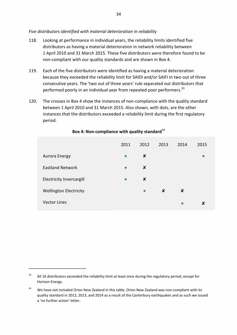
34

Five distributors identified with material deterioration in reliability

118. Looking at performance in individual years, the reliability limits identified five

distributors as having a material deterioration in network reliability between

1 April 2010 and 31 March 2015. These five distributors were therefore found to be

non‐compliant with our quality standards and are shown in Box 4.

119. Each of the five distributors were identified as having a material deterioration

because they exceeded the reliability limit for SAIDI and/or SAIFI in two out of three

consecutive years. The ‘two out of three years’ rule separated out distributors that

performed poorly in an individual year from repeated poor performers.33

120. The crosses in Box 4 show the instances of non‐compliance with the quality standard

between 1 April 2010 and 31 March 2015. Also shown, with dots, are the other

instances that the distributors exceeded a reliability limit during the first regulatory

period.

Box 4: Non‐compliance with quality standard34

2011 2012 2013 2014 2015

Aurora Energy ● ✘ ●

Eastland Network ● ✘

Electricity Invercargill ● ✘

Wellington Electricity ● ✘ ✘

Vector Lines ● ✘

33 All 16 distributors exceeded the reliability limit at least once during the regulatory period, except for

Horizon Energy.

34 We have not included Orion New Zealand in this table. Orion New Zealand was non‐compliant with its

quality standard in 2012, 2013, and 2014 as a result of the Canterbury earthquakes and as such we issued

a ‘no further action’ letter.

35

121. Box 4 reflects compliance with the quality standards as opposed to average

performance over the regulatory period, which was shown in Figure 22 and

Figure 23. For example, Alpine Energy had a 5 year average annual SAIDI above the

annual limit because the limit was exceeded by a material amount in 2011 and 2014.

However, the two years between 2011 and 2014 were below the limit. Therefore,

Alpine Energy did not break the ‘two out of three year’ rule.

122. Likewise a distributor could be found to be non‐compliant with the quality standard

owing to performance in two out of three years, even if performance over the 5 year

period was within the limit. This is because the limit is intended to allow for a degree

of natural variation. The quality standard identifies businesses where performance

falls outside the range of natural variability in two out of three years.

Responses to non‐compliance

123. Our options for enforcement responses to non‐compliance with the quality standard

range from issuing a ‘no further action’ letter through to seeking a penalty in Court.

We select the appropriate response by assessing our enforcement criteria: extent of

detriment; seriousness of conduct; and public interest.

124. We have already issued warning letters to Aurora, Eastland, and Electricity

Invercargill in response to those instances of non‐compliance.35 Our engineering

advisors raised concerns about Eastland and Aurora’s asset management (but not

Electricity Invercargill’s). Further breaches of quality standards by Eastland or Aurora

may therefore lead to stronger enforcement responses in the future.

125. For the remaining two instances of non‐compliance:

125.1 we are soon to complete our review of the causes and conduct associated

with the two instances of non‐compliance by Wellington Electricity; and

125.2 we are currently considering the findings of the Electricity Authority’s investigation into the 2014 Penrose substation fire, which contributed to the

non‐compliance reported by Vector Lines in 2015.

126. The asset management practices employed by these two distributors have added

significance given that together they serve around 34% of electricity consumers in

New Zealand.

35 Further information on our enforcement responses—including the warning letters and investigation

reports from our engineering advisors—is available on our website.

36

6. Comparison with other distributors

Purpose of chapter

127. This chapter provides a comparison of profitability, investment, and quality between

distributors affected by the November 2012 decision and other distributors in the

sector.

Comparison with other distributors provides useful context

128. A comparison with other distributors is useful for understanding the performance of

the distributors affected by our November 2012 decision in the context of the wider

sector. The other distributors include those that are only subject to information

disclosure regulation, and Orion New Zealand which is currently subject to a

customised price‐quality path.

129. As explained in the Introduction, there is less concern about profitability of

distributors that are only subject to information disclosure regulation, because

additional profits flow back to consumers in their role as owners. Customers can also

vote for the members of the Board of the Trusts which own and direct the

distributors.

Profitability of distributors affected by November 2012 decision was similar to others

130. Figure 24 shows that, with only a few exceptions, the profitability of distributors

affected by our November 2012 decision was broadly similar to other distributors

from 1 April 2012 to 31 March 2015. The distributors affected by our

November 2012 decision are shown as blue bars, Orion New Zealand is shown as the

orange bar, and other distributors are shown as green bars.36

36 As noted in Chapter 2, Orion New Zealand were not subject to the revenue limit adjustments in 2012 and

instead applied for a customised price‐quality path, which came into effect from 1 April 2014.

37

2504924.17

Figure 24: Nominal internal rate of return 2013‐15 (%) Figure 25: Nominal returns of distributors affected by November 2012 decision compared to other distributors37

37 The boxes show the range of the middle two quartiles (divided by the median) and the vertical lines show the range of the top and bottom quartiles.

0 1 2 3 4 5 6 7 8 9 10

Scanpower

Electra

Network Tasman

Alpine Energy


Nelson Electricity

MainPower

Counties Power

OtagoNet

Orion NZ

Powerco

Vector Lines


Waipa Networks

Unison Networks


Horizon Energy

Aurora Energy

WEL Networks

Northpower

Eastland Network

Top Energy

Centralines

The Lines Company

The Power Company

Buller Electricity

Network Waitaki

Westpower

Marlborough Lines

Default price‐quality path

Information disclosure only

Customised price‐quality path

0%

1%

2%

3%

4%

5%

6%

7%

8%

9%

10%

Price‐quality regulated Information disclosure

38

2504924.17

Figure 26: Percentage change in average annual expenditure between 2008‐2012 and 2013‐15

Operating expenditure38 Capital expenditure

38 Operating expenditure includes pass through and recoverable costs.

‐40 ‐30 ‐20 ‐10 0 10 20 30 40

The Lines Company

OtagoNet

Centralines


Eastland Network

Alpine Energy

Unison Networks

Buller Electricity

MainPower NZ

Network Waitaki

The Power Company

Vector Lines

Electra

Aurora Energy

Orion NZ

Westpower

Network Tasman

WEL Networks

Nelson Electricity


Powerco

Scanpower

Horizon Energy

Top Energy

Counties Power

Waipa Network

Northpower


Marlborough Lines




‐50 0 50 100 150 200 250 300 350

Nelson Electricity

MainPower NZ

Top Energy

Network Tasman

Eastland Network

Scanpower

Counties Power

Orion NZ


Horizon Energy

Alpine Energy

Northpower

Waipa Network

Network Waitaki

OtagoNet

Buller Electricity

WEL Networks

The Power Company

Powerco


Vector Lines

The Lines Company

Unison Networks


Electra

Aurora Energy

Marlborough Lines

Centralines

Westpower




39

2504924.17

Reliability was also similar to other distributors

131. This section presents the reliability of all distributors and the change in reliability

from previous levels. The measures of reliability, SAIDI and SAIFI, represent the

duration and frequency of interruptions respectively (as described in Chapter 5).39

132. Figure 27 and Figure 28 show that reliability levels are generally similar between the

two main groupings of distributors. However, there are large differences at the

individual distributor level. The potential causes of these differences are described in

Chapter 5.

39 The SAIDI and SAIFI measures have not been normalised for this chapter.

40

2504924.17

Figure 27: Average duration of interruptions per connection per year (average SAIDI minutes, 2011‐15)

Figure 28: Change in average duration of interruptions per connection per year (% change 2003‐10 to 2011‐15)

0 200 400 600 800


Nelson Electricity

Network Waitaki


WEL Networks

Scanpower

Electra

Aurora Energy

Counties Power

Unison Networks

Network Tasman

Waipa Network

Centralines

Horizon Energy

Orion NZ

Northpower

Vector Lines

The Power Company

Marlborough Lines

Powerco

Westpower

The Lines Company

Alpine Energy

Eastland Network

OtagoNet


MainPower NZ

Top Energy

Buller Electricity




‐100 ‐50 0 50 100 150 200 250

Buller Electricity

MainPower NZ

Orion NZ


Vector Lines

Top Energy

Westpower


Aurora Energy

The Power Company

Counties Power

Alpine Energy

Scanpower

Horizon Energy

Network Tasman

Eastland Network

Unison Networks

WEL Networks

Powerco

Marlborough Lines

OtagoNet

Waipa Network

Nelson Electricity

Centralines

Northpower

The Lines Company


Electra

Network Waitaki




41

Figure 29: Average number of interruptions per connection per year (average annual SAIFI, 2011‐15)

Figure 30: Change in average number of interruptions per connection per year (% change 2003‐10 to 2011‐15)

0 1 2 3 4 5 6



Nelson Electricity

Orion NZ

Network Waitaki

Scanpower

WEL Networks

Vector Lines

Aurora Energy

Network Tasman

Alpine Energy

Electra

Marlborough Lines

Waipa Network

Unison Networks

MainPower NZ

Buller Electricity


Horizon Energy

Powerco

Counties Power

Northpower

Westpower

OtagoNet

The Power Company

Centralines

Eastland Network

The Lines Company

Top Energy




‐50 0 50 100

Orion NZ

MainPower NZ


Scanpower

Buller Electricity

Westpower

Horizon Energy

Eastland Network


Nelson Electricity

Alpine Energy

Counties Power

Network Tasman


Aurora Energy

Top Energy

OtagoNet

The Lines Company

Unison Networks

The Power Company

Vector Lines

Electra

Northpower

Powerco

WEL Networks

Network Waitaki

Marlborough Lines

Centralines

Waipa Network




42

2504924.17

7. Conclusions and next steps

Purpose of chapter

133. This chapter explains the conclusions we have reached based on the findings

presented in this paper, and outlines what we expect to do next.

Key findings from this report

134. The key findings from our analysis of the profitability of electricity distributors are:

134.1 the adjustments we announced in November 2012 were effective at limiting

excessive profits and supporting investment incentives;

134.2 the return that distributors earned is comprised of a performance‐related

real return plus compensation for actual inflation; and

134.3 the profitability of individual distributors varied under the revenue limits, but

on average the forecasts we relied on in November 2012 performed well.

135. In addition, we have not found any evidence to suggest that the revenue limits

created barriers to investment in the network. However, we have stopped short of

assessing whether the increased expenditure was efficient.

Reflections on the variances

136. Although the forecasting approaches appear to have performed well, we consider

that the analysis raises some questions for us to address in future. These questions

relate to the variances for:

136.1 capital expenditure, which showed the biggest individual variation between the forecast and actual outcome for a relatively small distributor; and

136.2 billed quantities, which had a material impact on the returns earned by

certain distributors, without necessarily reflecting any changes in

performance, or better outcomes for consumers.

137. Reliably forecasting capital expenditure is difficult, especially when a small number

of projects can lead to large changes in spending. Therefore, for small distributors

specifically, we could:

137.1 consider the confidence we can have in distributor forecasts for future resets;

137.2 consider the exposure of profits to changes in capital expenditure under the Incremental Rolling Incentive Scheme; and

137.3 consider whether and how customised price‐quality paths could be made to be a more viable option.

43

138. Forecasting the impact of changes in quantities billed has its own challenges, and

these are likely to grow towards future resets. For example:

138.1 the five‐year forecast developed in 2012 relied on actual information for certain factors (such as Gross Domestic Product), whereas in future the five‐year forecast will rely exclusively on forecast data; and

138.2 the emergence of new technologies may make the impacts on revenue more difficult to predict given that past relationships between revenue and the factors that drive demand may no longer hold.

139. These difficulties are not insurmountable, but will need to be factored into our

future work.

Review of input methodologies provides opportunity to better promote Part 4

140. Most immediately, the analysis contained in this report may help inform our work on

the review of input methodologies. Amongst other things, this work includes

consideration of:

140.1 requirements for customised price‐quality path proposals;

140.2 form of control; and

140.3 inflation indexation of asset values.

141. We will also be reviewing all other matters covered by input methodologies, which

may have implications for future assessments of profitability, eg, the review of the

parameters for estimating cost of capital which is used to set and assess returns.

Incremental improvements introduced in November 2014

142. The review of input methodologies follows a number of incremental improvements

introduced before default price‐quality paths were reset in November 2014. These

incremental improvements included the introduction of:

142.1 the Incremental Rolling Incentive Scheme which will change the impact on

returns of differences between forecast and actual expenditure;

142.2 a new mechanism to better treat pass‐through and recoverable costs, to

eliminate the risk that may have resulted in some distributors pricing beneath

the limit to avoid inadvertent breaches; and

142.3 a new mechanism to ‘wash up’ for the difference between forecast and

actual capital expenditure prior to the start of the regulatory period.

44

143. We also made changes to our approaches for forecasting expenditure and revenue

growth, and selected the cost of capital from the 67th percentile of the estimated

WACC range rather than the 75th.

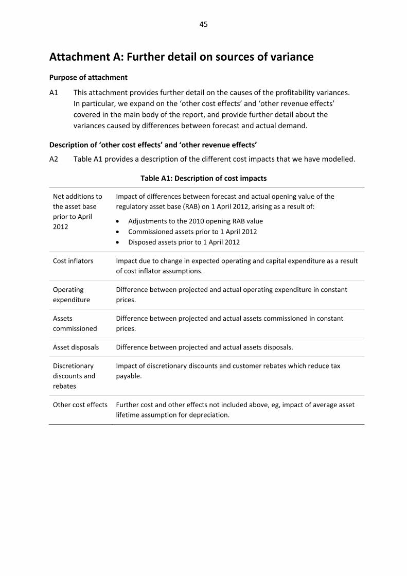
45

Attachment A: Further detail on sources of variance

Purpose of attachment

A1 This attachment provides further detail on the causes of the profitability variances.

In particular, we expand on the ‘other cost effects’ and ‘other revenue effects’

covered in the main body of the report, and provide further detail about the

variances caused by differences between forecast and actual demand.

Description of ‘other cost effects’ and ‘other revenue effects’

A2 Table A1 provides a description of the different cost impacts that we have modelled.

Table A1: Description of cost impacts

Net additions to

the asset base

prior to April

2012

Impact of differences between forecast and actual opening value of the

regulatory asset base (RAB) on 1 April 2012, arising as a result of:

Adjustments to the 2010 opening RAB value

Commissioned assets prior to 1 April 2012

Disposed assets prior to 1 April 2012

Cost inflators Impact due to change in expected operating and capital expenditure as a result

of cost inflator assumptions.

Operating

expenditure

Difference between projected and actual operating expenditure in constant

prices.

Assets

commissioned

Difference between projected and actual assets commissioned in constant

prices.

Asset disposals Difference between projected and actual assets disposals.

Discretionary

discounts and

rebates

Impact of discretionary discounts and customer rebates which reduce tax

payable.

Other cost effects Further cost and other effects not included above, eg, impact of average asset

lifetime assumption for depreciation.

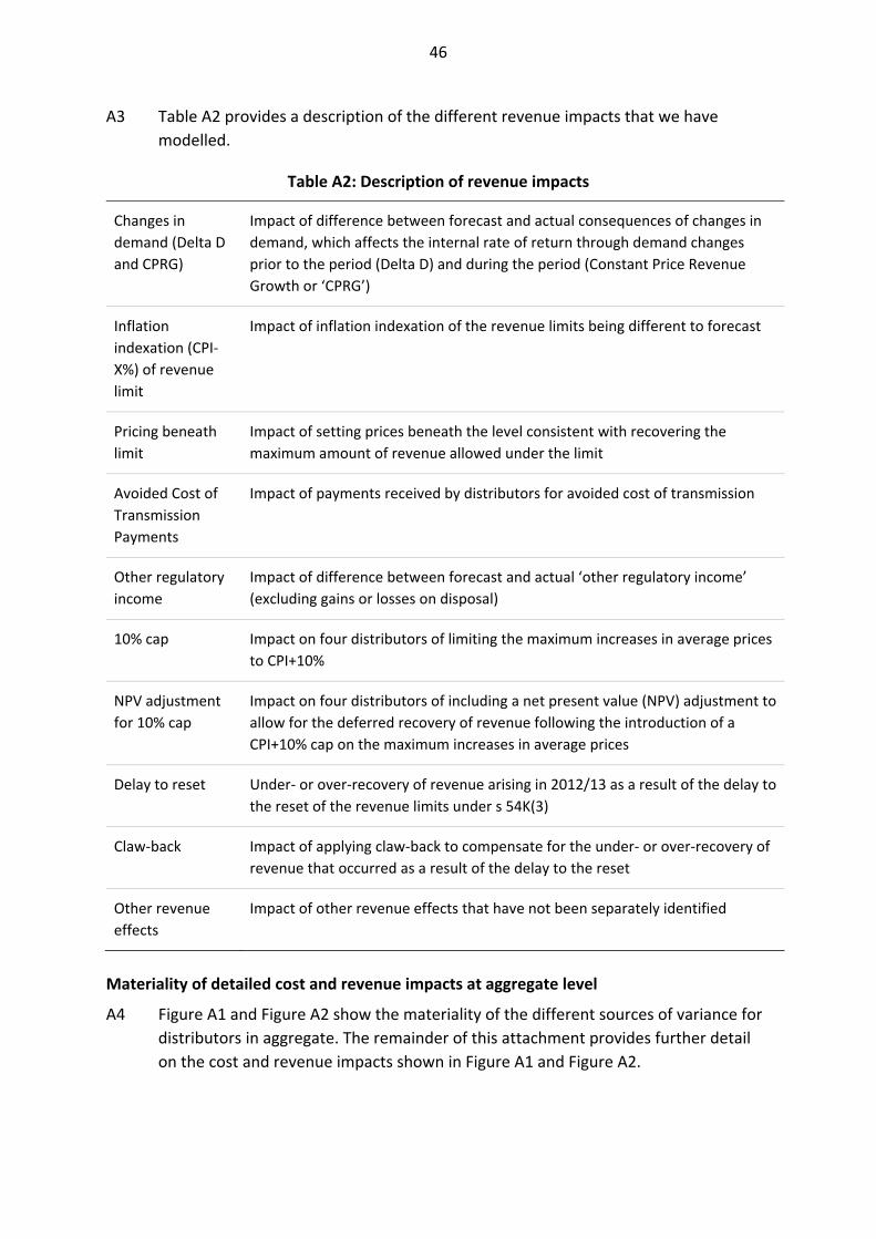
46

A3 Table A2 provides a description of the different revenue impacts that we have

modelled.

Table A2: Description of revenue impacts

Changes in

demand (Delta D

and CPRG)

Impact of difference between forecast and actual consequences of changes in

demand, which affects the internal rate of return through demand changes

prior to the period (Delta D) and during the period (Constant Price Revenue

Growth or ‘CPRG’)

Inflation

indexation (CPI‐

X%) of revenue

limit

Impact of inflation indexation of the revenue limits being different to forecast

Pricing beneath

limit

Impact of setting prices beneath the level consistent with recovering the

maximum amount of revenue allowed under the limit

Avoided Cost of

Transmission

Payments

Impact of payments received by distributors for avoided cost of transmission

Other regulatory

income

Impact of difference between forecast and actual ‘other regulatory income’

(excluding gains or losses on disposal)

10% cap Impact on four distributors of limiting the maximum increases in average prices

to CPI+10%

NPV adjustment

for 10% cap

Impact on four distributors of including a net present value (NPV) adjustment to

allow for the deferred recovery of revenue following the introduction of a

CPI+10% cap on the maximum increases in average prices

Delay to reset Under‐ or over‐recovery of revenue arising in 2012/13 as a result of the delay to

the reset of the revenue limits under s 54K(3)

Claw‐back Impact of applying claw‐back to compensate for the under‐ or over‐recovery of

revenue that occurred as a result of the delay to the reset

Other revenue

effects

Impact of other revenue effects that have not been separately identified

Materiality of detailed cost and revenue impacts at aggregate level

A4 Figure A1 and Figure A2 show the materiality of the different sources of variance for

distributors in aggregate. The remainder of this attachment provides further detail

on the cost and revenue impacts shown in Figure A1 and Figure A2.

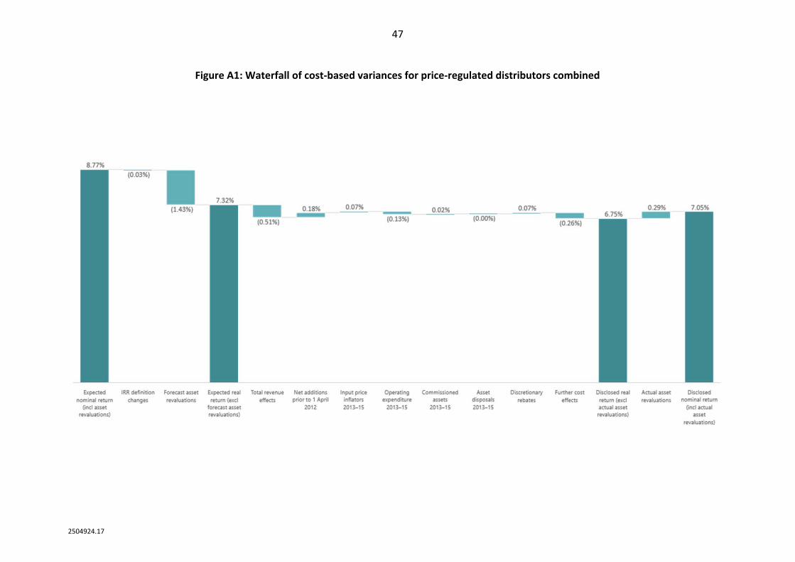
47

2504924.17

Figure A1: Waterfall of cost‐based variances for price‐regulated distributors combined

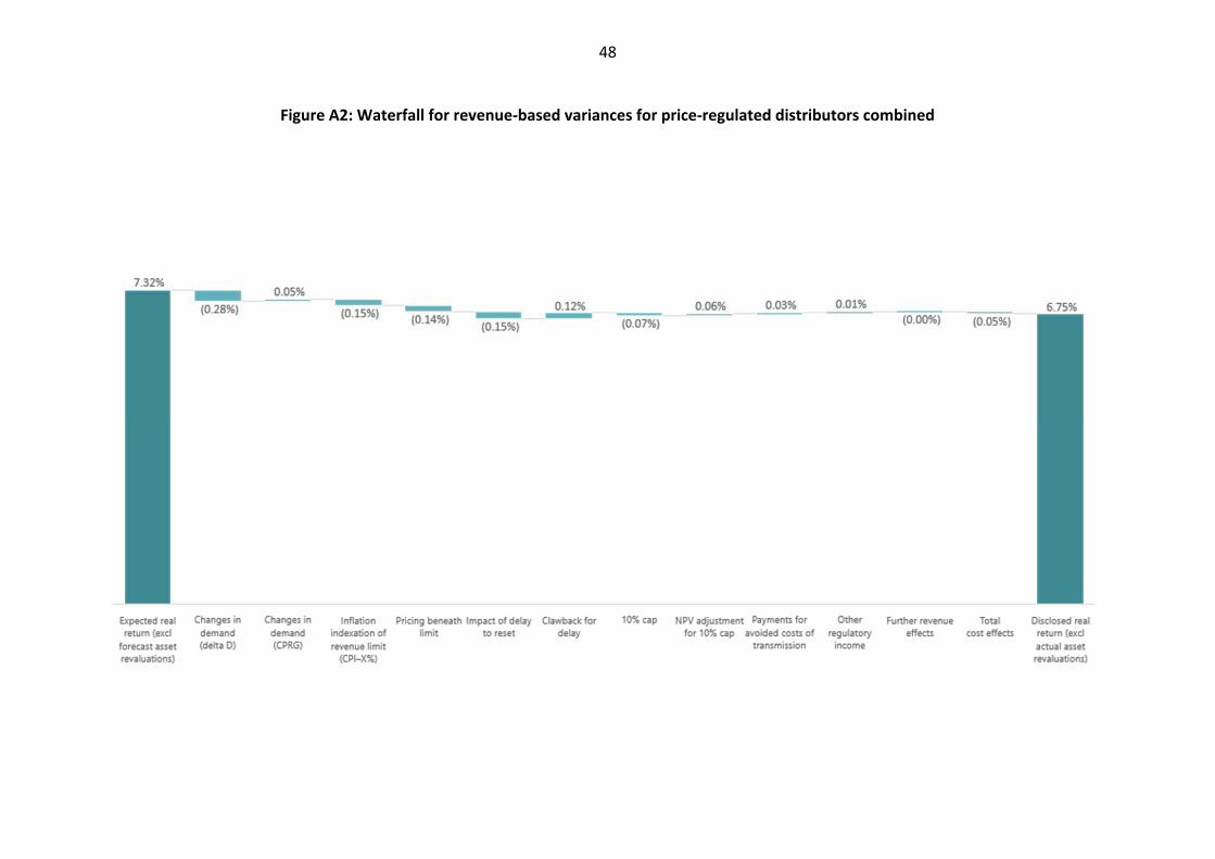
48

Figure A2: Waterfall for revenue‐based variances for price‐regulated distributors combined

49

2504924.17

Pricing beneath limit

A5 To varying degrees, all distributors set average prices that were below the maximum

allowed under the revenue limit. When we adjusted the revenue limits, however, we

assumed that distributors would set average prices as high as possible in order to

maximise revenue and profitability.

A6 Figure A3 shows that the differences in some cases were large, with three

distributors setting average prices that were more than 10% below the maximum.40

For most distributors, the differences were quite small, between 0% and 2%.

A7 Importantly, Figure A3 and Figure A4 reflect the impact of pricing beneath the limit

in only the last two of the three years examined in this report. This is because of the

way we specified the approach to claw‐back, which allowed distributors to recover

any shortfall arising in the first of the three years.41

A8 For the three distributors most affected—Network Tasman, Centralines, and The

Lines Company—the difference was equivalent to more than one percentage point

of returns. In the case of Network Tasman, returns would therefore have been as

high as 9.38% if prices had been set consistent with the revenue limit.

40 For the purposes of this report, we have calculated ‘pricing below the limit’ as the percentage difference

between actual notional revenue and allowable notional revenue. Our calculation of the amount that the

distributors have priced below the limit is therefore based on their self‐reported compliance position.

41 Notably, Wellington Electricity set prices 2.0% lower due to an error in the calculation of the inflation

indexation of the revenue limit. Our clawback decision allowed Wellington Electricity to increase prices in

later years to recover this shortfall.

50

Figure A3: Difference between allowed and actual revenue (%)

Figure A4: Impact on returns of pricing below limit (percentage points)

A9 The reasons for pricing significantly beneath the limit may be explained, at least in

part, by the ownership arrangements in place for the three distributors. All three

distributors appear to have set prices with the impacts on consumers in mind. This

suggests that consumer‐ownership may have played a role.

A10 In addition, these distributors and others may have set prices beneath the limit to

provide a buffer against the risk of non‐compliance with the revenue limits. For

example, the buffer may reflect issues associated with the way pass‐through and

recoverable costs were recovered during the last regulatory period.42

A11 The issues associated with pass‐through and recoverable costs were that:

A11.1 distributors were required to forecast pass‐through and recoverable costs,

which they have found difficult in practice; and

A11.2 the recovery of the amounts required to cover pass‐through and

recoverable costs were associated with some degree of volume risk.

A12 Notably, despite these issues, a number of distributors were still able to price quite

close to the limit, eg, Vector Lines and Unison Networks.

42 These issues have been addressed in the way the revenue limits are specified for the 2015‐20 regulatory

period.

‐20 ‐15 ‐10 ‐5 0

Vector Lines

Unison Networks


Eastland Network

Horizon Energy

Aurora Energy

Powerco

OtagoNet


Nelson Electricity

Alpine Energy

Centralines


Network Tasman

Top Energy

The Lines Company

‐2.0 ‐1.5 ‐1.0 ‐0.5 0.0

Vector Lines

Unison Networks


Eastland Network

Horizon Energy

Aurora Energy

Powerco

OtagoNet


Nelson Electricity

Alpine Energy

Centralines


Network Tasman

Top Energy

The Lines Company

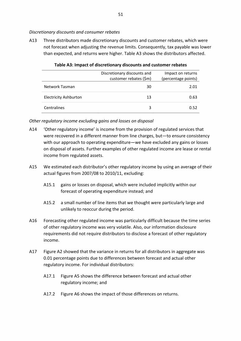
51

Discretionary discounts and consumer rebates

A13 Three distributors made discretionary discounts and customer rebates, which were

not forecast when adjusting the revenue limits. Consequently, tax payable was lower

than expected, and returns were higher. Table A3 shows the distributors affected.

Table A3: Impact of discretionary discounts and customer rebates

Discretionary discounts and customer rebates ($m)

Impact on returns (percentage points)

Network Tasman 30 2.01

Electricity Ashburton 13 0.63

Centralines 3 0.52

Other regulatory income excluding gains and losses on disposal

A14 ‘Other regulatory income’ is income from the provision of regulated services that

were recovered in a different manner from line charges, but—to ensure consistency

with our approach to operating expenditure—we have excluded any gains or losses

on disposal of assets. Further examples of other regulated income are lease or rental

income from regulated assets.

A15 We estimated each distributor’s other regulatory income by using an average of their

actual figures from 2007/08 to 2010/11, excluding:

A15.1 gains or losses on disposal, which were included implicitly within our

forecast of operating expenditure instead; and

A15.2 a small number of line items that we thought were particularly large and

unlikely to reoccur during the period.

A16 Forecasting other regulated income was particularly difficult because the time series

of other regulatory income was very volatile. Also, our information disclosure

requirements did not require distributors to disclose a forecast of other regulatory

income.

A17 Figure A2 showed that the variance in returns for all distributors in aggregate was

0.01 percentage points due to differences between forecast and actual other

regulatory income. For individual distributors:

A17.1 Figure A5 shows the difference between forecast and actual other

regulatory income; and

A17.2 Figure A6 shows the impact of those differences on returns.

52

A18 A few of the distributors (such as Aurora Energy) received particularly higher than

expected other regulatory income, which increased their profitability.

Figure A5: Difference between forecast and actual other regulatory income ($m)

Figure A6: Impact on returns of other regulatory income (percentage points)

‐20 ‐10 0 10

Aurora Energy

Nelson Electricity

OtagoNet

Top Energy

Centralines

Network Tasman

Unison Networks

Horizon Energy



Powerco

Alpine Energy

The Lines Company


Eastland Network

Vector Lines

‐0.2 0.0 0.2 0.4 0.6

Aurora Energy

Nelson Electricity

OtagoNet

Top Energy

Centralines

Network Tasman

Unison Networks

Horizon Energy



Powerco

Alpine Energy

The Lines Company


Eastland Network

Vector Lines

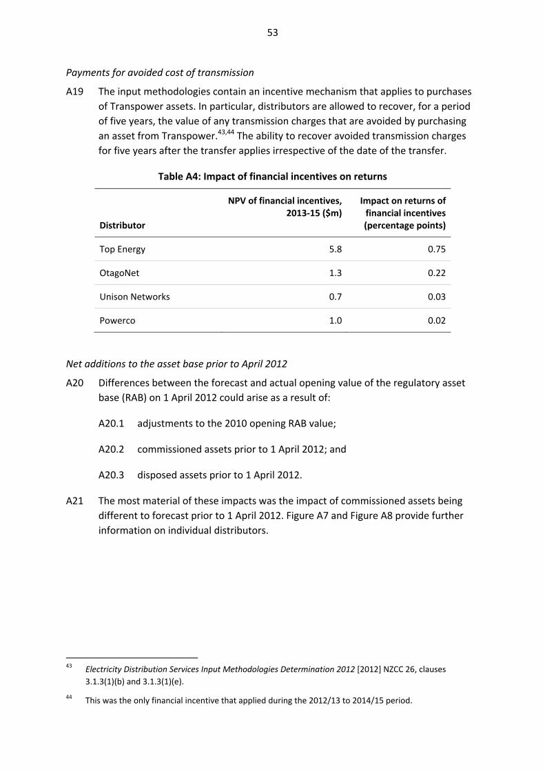
53

Payments for avoided cost of transmission

A19 The input methodologies contain an incentive mechanism that applies to purchases

of Transpower assets. In particular, distributors are allowed to recover, for a period

of five years, the value of any transmission charges that are avoided by purchasing

an asset from Transpower.43,44 The ability to recover avoided transmission charges

for five years after the transfer applies irrespective of the date of the transfer.

Table A4: Impact of financial incentives on returns

Distributor

NPV of financial incentives, 2013‐15 ($m)

Impact on returns of financial incentives (percentage points)

Top Energy 5.8 0.75

OtagoNet 1.3 0.22

Unison Networks 0.7 0.03

Powerco 1.0 0.02

Net additions to the asset base prior to April 2012

A20 Differences between the forecast and actual opening value of the regulatory asset

base (RAB) on 1 April 2012 could arise as a result of:

A20.1 adjustments to the 2010 opening RAB value;

A20.2 commissioned assets prior to 1 April 2012; and

A20.3 disposed assets prior to 1 April 2012.

A21 The most material of these impacts was the impact of commissioned assets being

different to forecast prior to 1 April 2012. Figure A7 and Figure A8 provide further

information on individual distributors.

43 Electricity Distribution Services Input Methodologies Determination 2012 [2012] NZCC 26, clauses

3.1.3(1)(b) and 3.1.3(1)(e).

44 This was the only financial incentive that applied during the 2012/13 to 2014/15 period.

54

Figure A7: Difference between forecast and actual capex prior to 1 April 2012 (%)

Figure A8: Impact on returns of difference between forecast and actual capex prior to

1 April 2012 (percentage points)

Delay to reset and claw‐back for delay

A22 The impact of the delay to the reset was largely offset by claw‐back for the delay

(when assessed using the cost of debt as the interest rate). The reason for a slight

difference at the aggregate level is that claw‐back was not provided for The Lines

Company in the next regulatory period. This is because The Lines Company provided

incorrect information in response to the information gathering request we issued

ahead of the November 2012 reset.45

CPI+10% cap and net present value adjustment for ten percent cap

A23 Alongside our decision to apply a CPI+10% cap to the maximum increases in average

prices, which affected four distributors, we also committed to allowing additional

recovery of revenue in the next regulatory period. This had the effect of spreading

the most significant price increases over a longer time period. The two effects offset

each other in NPV terms (when assessed using the cost of debt as the interest rate).

45 For further information, refer: Chapter 5 of Commerce Commission “Default price‐quality paths for

electricity distributors from 1 April 2015 to 31 March 2020: Main policy paper”, 28 November 2014.

‐100 ‐50 0 50 100

Nelson Electricity

Alpine Energy

Network Tasman

Horizon Energy

OtagoNet

Unison Networks


Aurora Energy

Top Energy


Powerco

Vector Lines

The Lines Company

Eastland Network


Centralines

‐1 0 1 2 3

Nelson Electricity

Alpine Energy

Network Tasman

Horizon Energy

OtagoNet

Unison Networks


Aurora Energy

Top Energy


Powerco

Vector Lines

The Lines Company

Eastland Network


Centralines

55

Attachment B: Calculations

Purpose of attachment

B1 This attachment explains how we calculated the profitability of each supplier, and

variances from our assumptions, using internal rate of return analysis.

Internal rate of return calculations

B2 In this section we explain:

B2.1 the internal rate of return formula that we used;

B2.2 the inputs that we used;

B2.3 simplifications and assumptions that we made; and

B2.4 differences to the internal rate of return formula in information disclosure.

B3 The other section of this attachment explains how we calculated the profitability

variances (presented in Chapters 3 and 4).

Internal rate of return formula

B4 Our analysis relied on the standard formula for calculating an internal rate of return

(IRR) over a particular period—in our case 1 April 2012 to 31 March 2015—based on

three components:

B4.1 opening asset value;

B4.2 cash flows during the period; and

B4.3 closing asset value.

B5 The IRR is the discount rate that would make the net present value of the three

components equal to zero.

56

Opening asset value

B6 We considered the opening asset value to be the opening regulated asset base plus

the value of deferred tax. Both of these terms are defined in the electricity

distribution services input methodology (regulated asset base is abbreviated as RAB

in the input methodology).46

Cash flows during the period

B7 We considered several categories of incoming and outgoing cash flows (ie, revenues

and costs) for calculation of the IRR.

B8 The incoming cash flows—the total regulatory income less pass‐through costs and

recoverable costs—that we considered were categorised as:

B8.1 revenue recovered under the price limit;

B8.2 other regulator income (excluding gains and losses on disposals); and

B8.3 revenue adjustments made during the period for claw‐back.

B9 The outgoing cash flows that we considered were categorised as:

B9.1 operating expenditure;47

B9.2 capital expenditure; and

B9.3 tax payable.

Closing asset value

B10 We calculated the closing asset value as the sum of:

B10.1 the regulated asset base;

B10.2 deferred tax;

B10.3 outstanding claw‐back amounts; and

B10.4 any net present value adjustment required in the next regulatory period.48

46 Commerce Commission “Electricity Distribution Services Input Methodologies Determination 2012;

consolidating all amendments as of 15 December 2015” (3 February 2016).

47 Owing to the way operating expenditure was forecast in November 2012, we included gains and losses on disposal when modelling the impact of differences in operating expenditure.

48 To give deferred clawbacks a neutral impact in real terms we add an adjustment by applying the debt rate

to the clawback.

57

General approach for calculating variances

B11 To assess the impact of any differences—such as actual and forecast operating

expenditure—we used the financial model to calculate the profitability for each of

the two scenarios. The difference between the two resulting internal rates of return

is what we considered to be the impact of the variance.

B12 For some of the variances we had to run scenarios as if we had perfect foresight for

some inputs in the financial model. This required recalculation of the regulated asset

base roll forward. The opening and closing regulated asset base values were also

affected by the depreciation and revaluation effects.

An exception—how we calculated the impact of actual asset revaluations

B13 To calculate the impact of actual asset revaluations, instead of applying actual

inflation in the financial model for the revaluation of the regulated asset base, we

applied forecast inflation to the regulated asset base value disclosed and rolled

forward under information disclosure.

B14 The regulated asset base value disclosed by distributors reflects actual capital

expenditure, disposals, and depreciation rates. Consequently, our approach to

calculating the effect of actual asset revaluations produces a better estimate than

comparing two scenarios of the financial model with actual and forecast inflation.

Relationship with profitability indicator under information disclosure regulation

B15 For the analysis presented in this paper we have calculated profitability in largely the

same way as the improved profitability indicator disclosed by distributors since the

March 2015 amendments to the information disclosure requirements. Specifically,

this is the return on investment indicator with mid‐year cashflow timing reflecting all

revenue earned. This means that it is not equivalent to the profitability indicator

disclosed during 2012/13 to 2014/15.

B16 The main improvement in the profitability indicator is that it now includes revenue

from financial incentives and wash‐ups like the avoided transmission recoverable

cost. The other improvements were changes to the timing assumptions, such as

when line charge revenue was assumed to be received. Some of these other

improvements explain why we have calculated the nominal target return to be

8.73% to 8.77% (depending on the distributor) rather than the 8.77% that was

originally used for setting the default price‐quality path.

Summary and analysis - comcom.govt.nz · X2 Majority of distributors within one percentage point of...

Documents

Transcript of Summary and analysis - comcom.govt.nz · X2 Majority of distributors within one percentage point of...