Sumedha Bajar - cesifo-group.de · Sumedha Bajar I. Introduction Achieving balanced economic growth...

THE INFRASTRUCTURE-OUTPUT NEXUS: REGIONAL EXPERIENCE FROM INDIA

Sumedha Bajar

Designation: Doctoral Student

Affiliation: Institute for Social and Economic Change

Address : ISEC PhD Scholars’ Hostel

ISEC, Nagarbhavi, Bangalore

Karnataka – 560072

e-mail: [email protected]; [email protected]

Mobile no. : 07829376006

The Infrastructure-Output Nexus: Regional Experience from India

Sumedha Bajar

mailto:[email protected]

mailto:[email protected]

1


Sumedha Bajar

Abstract

Infrastructure plays an important role to support development and growth. In recent years

India has come to enjoy the reputation of fast growing developing nation. In order to ensure

that nothing hinders this growth process or its furtherance it is important to identify the

major bottlenecks to growth and the channels through which they may operate. In this paper

attempts are made to establish the nexus between per capita NSDP in India and

infrastructure availability in the 17 major Indian states. The main conclusions that can be

drawn are: considerable regional disparities exist in terms of per capita net state domestic

product (PCNSDP) for the time period 1981 to 2010. These disparities have increased over

the years even though the initially poor states have been growing at faster rate. After

grouping the states into three categories important observations were that the poor states

were also the ones with least amount of infrastructure development, whereas, the rich states

had relatively much better infrastructure provision but there is evidence of an increase in

infrastructure growth in poor states after the reforms of 1991 even though their level still

remained considerably below that of the rich states. After undertaking panel data estimation

it was found physical infrastructure variables did not have a uniform influence on output.

The relationship not just differed for aggregate output, secondary and tertiary sector output;

there was also distinct difference in the impact infrastructure had on the same sector for

different time periods. This paper is part of on-going research exercise aiming at a

comprehensive empirical work exclusive to India that can help identify the role

infrastructure development.

JEL codes: H54, O11, L92, L94, L96,O53

Keywords: Physical Infrastructure, Output (NSDP), Economic Development, India

20th

June, 2012

I would like to acknowledge and thank CESifo GmbH, Munich, Germany for providing me

the opportunity to present this paper at the CESifo Venice Summer Institute 2013 workshop

on “The Economics of Infrastructure Provisioning: The (Changing) Role of the State”

taking place at Venice International University on the island of San Servolo, Venice, Italy

on the 26 and 27 July 2013

2


Sumedha Bajar

I. Introduction

Achieving balanced economic growth amongst the Indian states has been a persistent aim of

the Indian government and the planners since Independence. Economic policies that helped

in promoting economic growth with equity and minimising inter-regional disparities formed

the major thrust of planning process. But despite having common political institutions and

national economic policies, these objectives have not been realised and considerable inter-

state disparities remain (Nair, 1993; Cashin and Sahay, 1996; Nagaraj, Varoudakis and

Veganzones, 2000 and Rao, Shand and Kalirajan, 1999 among others).

Although, India’s growth performance during the first thirty years of Independence had

been lacklustre (the term ‘Hindu rate of growth’ was disparagingly used to refer to the

modest growth rate experienced during this period), this pattern started showing a

change1980s with partial liberalization of the economy and more so with the wide-ranging

reforms which followed the balance of payment crisis in 1991. Gross domestic product

(GDP) grew on average at 5 per cent in the 1980s and increased further in the 1990s and

touched the 9 per cent mark in the second half of 2000s.

Even with these fast evolving changes at the national level, regional inequalities have

remained obstinate. In 1980-81, an average citizen of Punjab was four times richer than the

average citizen of Bihar. The situation has not changed much since. In 2009-10 the per

capita income level in Bihar (the poorest state in India) was still one fourth that of

Maharashtra (the richest state) and one third that of Punjab. Of the five initially poor states

(Bihar, Madhya Pradesh, Uttar Pradesh, Rajasthan and Andhra Pradesh) in 1980-81, four

still remained among the poorest (in per capita terms) in 2009-10 with the exception of

Andhra Pradesh. Interestingly, Maharashtra which had 8 per cent of total national

population contributed 16 per cent of the aggregate net state domestic product (NSDP) in

2009-10, while Bihar with more than 10 per cent of population contributed only 4.5 per

cent of the aggregate NSDP (See Table1A). Rising regional inequalities can have several

repercussions on both economic and political stability in the country (Nagaraj, Varoudakis

and Veganzones, 2000).

3

While reducing inter-state disparities in growth and income remain avowed objectives of

Indian planning for balanced regional development, reducing the real interest rate in the

economy and ensuring long run sustainable growth by reducing the fiscal deficit is of utmost

importance for both regional and national economy. The present system of fiscal federalism

mandates increased transfers from central government to the less developed states making it

even harder to reduce the federal deficit. In addition, with the rise in coalition politics, the

stability of central government is highly dependent on support from regional political

parties. Thus, achieving balanced growth and reducing regional disparities is a major

challenge that the Indian government faces.

In view of the above discussion, it becomes important to understand the determinants of

development of sub-national regions. The literature points to various set of strategies

through which the objective of balanced regional development can be accomplished. These

are industrial development, rural development, migration, infrastructure development,

subsidies to capital and labour, fiscal incentives, administrative decentralisation- to list a

few (Markusen 1994; Higgins and Savoie 1995 and Richardson and Townroe 1986).

Infrastructure provision is seen as a particular instrument for promoting regional

development in which the governments can play an important role due to the public goods

nature of infrastructure facilities. Services provided by infrastructure capital stock- power,

transport, telecommunication- are considered fundamental to economic activity by way of

serving as intermediate inputs and taking part in the production process. Furthermore,

infrastructure availability enhances long run growth performance by facilitating market

transactions and creating positive externalities among firms or industries that influence their

location decisions (Jumenez, 1995). Studies have also highlighted the productivity impact of

infrastructure by considering infrastructure investment as complementary to private

investments (Seitz and Licht 1992; Greene and Villanueva 1991). In the regions where

infrastructure facilities are developed entrepreneurs find it easier to adopt new technologies

and generate technical progress thus changing the competitive nature of the region and help

achieve economic growth. However, it may also happen that regions endowed with better

infrastructure and thus having comparative advantage, gain output at the expense of

neighbouring states by attracting the mobile factors of production away from other locations

(these are known in the literature as negative spillover effects) and increasing regional

disparities (Boarnet, 1997).

4

In this context, an examination of the precise economic relation of infrastructure and output

with respect to the Indian states would be of great use to policy makers and researchers.

This study analyses a panel of 17 major Indian states over the time period 1980- 2010

(except for telecommunications, the data for which is available from 1991 onwards). The

focus in this paper is on physical capital stocks in network sectors: transport (roads and

railways) and non-transport (electricity, telecommunications). All these sectors can be

expected to have network externalities and large economies of scale. Their expansion can be

fostering competition in other segments by facilitating market access through lowering the

costs of transport and communication. The impact of social infrastructure is excluded for

now and these will be added later to the study. The study begins the analysis by using basic

descriptive statistics followed by panel econometric techniques.

The remainder of the paper is structured as follows; a brief review of literature presented in

Section 2 serves to position this paper. An overview of inequalities in per capita income and

growth performance of Indian states is presented in Section 3. The same section summarises

the evolution of infrastructure availability at state-level. Section 4 presents the empirical

results obtained which focus on nature and strength of the relationship between

infrastructure and PCNSDP. The last section offers concluding remarks.

II. Brief Review of Literature

Until the late 1980s little attention was paid by the economists on the role of infrastructure

in either theoretical or empirical studies (Gramlich, 1994). Starting with the seminal work

by Aschauer (1989), public capital (or infrastructure) formed an element in the aggregate

production function. He examined the relation between aggregate productivity and stock and

flow government spending variable for the US economy for the time period 1949 to 1985

and concluded that non-military public capital stock yields very high returns( in the range of

60-100 per cent per annum). This sparked off a debate in the empirical literature focussing

on the technical issues such as the form of the production function used amongst others.

Probably the first study that included public capital in an empirical cross country growth

model was by Easterly and Rebelo (1993), who ran pooled regressions (using decade

averages for the 1960s, 1970s and 1980s) of per capita growth on (sectoral) public

investment and conditional variables for 36 countries(see Sturm et al, 1998 for a summary).

They found that the share of public investment in transport and communication

infrastructure is correlated with growth. Likewise, Gwartney et al. (2004) consider 94

5

countries during the time period 1980-2000 and find a significant positive effect of public

investment, although its coefficient is always smaller than that of private investment.

However, other studies using the public investment share of GDP as regressor report

different results. For instance, Sanchez-Robles (1998) explores empirically the relationship

between infrastructure and economic growth by including the data of expenditure in

infrastructure as a share of GDP in traditional growth cross-country regressions and find a

negative growth impact of infrastructure expenditure in a sample of 76 countries. In

addition, the paper elaborates some new indicators of investment in infrastructure

employing physical units of infrastructure. Devarajan et al. (1996) report evidence for 43

developing countries, indicating that the share of total government expenditure

(consumption plus investment) has no significant effect on economic growth. Their

empirical analysis makes use of annual data on 43 developing countries from 1970-1990 to

examine the link between components of government expenditure and economic growth.

Devarajan et al. attribute their results to the fact that excessive amounts of transport and

communication expenditures in those countries make them unproductive. Prichett (1996)

suggested another explanation, arguing that public investment in developing countries is

often used for unproductive projects. As a consequence, the share of public investment in

GDP can be a poor measure of the actual increase in economically productive public

capital.

Other important studies that have made use of either Cobb Douglas or trans log production

function, with different types of infrastructure as separate factors of production alongside

private physical capital and labour, at either cross country or national level are by Easterly

and Rebelo (1993), Everaert and Heylen (2004) Bonaglia et al. (2000), Cadot et al. (1999),

Canning (1999), Canning and Bennathan (2000), Charlot and Schmitt (1999) Calderon and

Severn (2002), Esfahani and Ramirez (2002) and report output elasticity of infrastructure

between 0.1 and 0.2. In contrast, paper by Bougheas, Demetriades and Mamuneas (1999)

introduced infrastructure as a cost-reducing technology in Romer’s model of endogenous

growth and provide evidence using data from US manufacturing industry that the degree of

specialisation is positively correlated with infrastructure stock availability.

The patterns of growth of the group of developed countries and the group of developing

nations have been found to be quite different. While income differentials between countries

are extremely large, income differentials within regions of a given country can also be

significant. In the case of India, Nair’s (1983) pioneering analysis covered 14 major states of

6

India and found that the inter-state disparities in per capita NSDP, as measured by

coefficient of variation (CV) had declined over the period 1950-51 to 1964-65, but increased

between 1964-65 and 1976-77. In Dandekar (1993) it was claimed that the inter-state

economic disparity increased rather than decreasing over time. Study by Mathur (2001)

reported a steep acceleration in the coefficient of variation of per capita incomes in the post-

reform period of 1991-96. The study also concluded that within the middle income states

there was a tendency towards convergence, while divergence was evident within the groups

of high and low income states. A comparative analysis of 15 major states in respect of a

variety of indicators was attempted by Kurian (2000). His study also drew attention to inter-

state disparities by presenting data for states on demographic characteristics, poverty ratio,

magnitude and structure of State Domestic Product (SDP), developmental and non-

developmental revenue expenditure, indicators of physical infrastructure development

and indicators of financial infrastructure amongst other variables.

A large part of the mainstream economic research on infrastructure (as mentioned above)

has concluded that the impact on growth is substantial and significant. In this context, it will

be worthwhile to look at the case of Indian states and consider the patterns and impact of

factors like infrastructure development in explaining inter-state differences in growth rate in

India. Ghosh and De (1998) have tried to identify the role of infrastructure in regional

development over the plan periods from 1971-72 till 1994-95. They tested the impact of

public investment and physical infrastructure on both private investment behaviour and

regional economic development using OLS regression. For this purpose, a physical

infrastructure development indicator was formulated by them using the principal component

analysis. The results of their study are significantly conclusive for the time period studied

and they conclude that there were increasing regional disparity in India and regional

imbalances in physical infrastructure are responsible for rising income disparity across the

states.

A related study by the same authors (2000) tried to find out the linkage between a composite

index of infrastructure development and income across Indian states. The index was

constructed using two different approaches (PCA and OLS) using ten infrastructural

variables for four different years across 26 Indian states. The years are 1971-72, 1981-82,

1991-92 and 1994-95. This study concluded that the rising inequality in ten important

infrastructure facilities was responsible for widening income disparity. Planned

disbursement of funds by the government had failed to cure this disparity.

7

Another study on the same lines by Ghosh and De (2004) tested the relationship of physical,

social and financial infrastructure with per capita income across states. Three separate

indices were created – Physical Infrastructure Development Index (PIDI), Social

Infrastructure Development Index (SIDI) and Financial Infrastructure Development Index

(FIDI). They conclude that infrastructurally better endowed states have remained in the

same position relative to their poorer counterparts and this sets limits to growth.

The study by Nagaraj, Varoudakis and Veganzones (2000) examined the growth

performance of Indian states during 1970-94. They started by grouping the states according

to differences in the availability of physical, social and economic infrastructure using

principal component analysis and assessed the contribution of various infrastructure

indicators to growth performance using PCA and panel data estimation techniques.

Instrumental variable estimation technique was applied to tackle the endogeneity issue in the

provision of infrastructure. This study finds persistent income inequalities amongst states

and accounts for these due to differences in structure of production, infrastructure

endowments and state specific fixed effects in growth regression.

On a different line, Lall (1999) has tried to examine the relationship between public

infrastructure investments and regional development in India. He concludes that leading,

intermediate and lagging states are structurally different and infrastructure investments

influence growth in these regions through different pathways. This study covers time period

1980-81 to 1993-94 and examines the development process of 15 states. Instead of using

physical indicators of infrastructure, the dependent variables in the study are – public

investments in economic infrastructure (transport, power, telecom and irrigation); public

investment in social infrastructure (education, water supply and sanitation, medical and

public health); private investment and private employment. A common result that emerged

across all states is that investments in social infrastructure have positive effects on regional

growth. This study failed to show any positive linkage between economic infrastructure

investments and regional economic growth. This could be due to the use of a simple uni-

directional causal model that fails to capture the multiple impact path-potentials between

infrastructure and growth.

At this juncture it will be appropriate to point out the research gaps that could be identified

in literature and bring the focus of this study in sight. First, not all studies find a uniform

growth-enhancing effect of public capital or infrastructure. Second, these studies have not

8

taken into account the presence of unit root in the data series and thus, the results are not

econometrically sound. With the rise of stationarity testing and correction in econometrics

the analysis needs to evolve and presence of unit roots must be taken account of. This paper

is an attempt to establish the link between physical infrastructure and state output by making

use of panel cointegration framework after testing for stationarity.

In the following two sections after providing evidence for existence of regional disparities in

income in India, identification of the role differences in infrastructure endowment played in

per capita income level and its growth in Indian states was attempted.

III. Economic Features of Indian States and Regional Disparities

There are big disparities in economic development and growth performance between states

in India. Understanding these is of paramount importance when one is trying to determine

the factors accounting for long run Indian growth trends. Attention is called to inequalities

in real per capita Net State Domestic Product (in 2004-05 prices) and analysis is presented

in the sub section B. Present study intends to examine the effect infrastructure has on level

of state output. For this purpose, certain infrastructure variables were selected as indicators

of infrastructure development and their trend analysed over time and across states in sub

section C. Most of these indicators are either absolutely government controlled or are

regulated either by central or state government. It must be noted that supply of infrastructure

is a stock available over discrete time points.

A. Data, Coverage of States and Time Period

India is a union of 28 states and 7 union territories but the analysis in this paper is confined

to only 17 major states -Andhra Pradesh, Assam, Bihar, Gujarat, Haryana, Himachal

Pradesh, Jammu and Kashmir, Karnataka, Kerala, Madhya Pradesh, Maharashtra, Orissa,

Punjab, Rajasthan, Tamil Nadu, Uttar Pradesh and West Bengal. The states of Chhattisgarh,

Jharkhand and Uttarakhand were treated as parts of the states from which they were carved

out in 2000 (Madhya Pradesh, Bihar and Uttar Pradesh, respectively). These 17 states

account for about 90 percent of national net domestic product (GDP), 92 percent of national

gross fixed capital formation (GFCF) and 93.5 percent of total labor force in 2009-10 and

are therefore representative.

The major economic variables used for this study are Net State Domestic Product (and

PCNSDP) and physical infrastructural variables - per capita electricity consumption (KwH),

9

Road density (km of surfaced road per 1000 sq. km of geographical area), Rail density (km

of rail length per 1000 sq km of geographical area) and Tele-density (per 10000 population).

The data was compiled from Ministry of Statistics and Programme Implementation

(MOSPI); Ministry of Road Transport and Highways, Govt. of India; various issues of

Statistical Abstract of India, GoI; and Economic Intelligence Service published by CMIE.

For tele-density state-wise data is available only 1991 onwards and Indiastats was accessed

for the compilation of the same.

The basic strategy employed in this paper is to divide the entire time period from 1980-2010

into three decades: 1980-1989; 1990-1999 and 2000-10 and to discern the impact of

infrastructure variables on levels of PCNSDP in the respective time period. The same was

repeated with sectoral PCNSDP- secondary and tertiary sector PCNSDP to examine the

differences in the impact of infrastructure development on levels of the respective sectoral

PCNSDP in the later sections.

B. Regional Disparity in per capita NSDP

There is a vast body of literature dealing with economic growth and its pattern in Indian

states (Nair,1983; RoyChoudhary, 1993; Cashin and Sahay, 1996; Rao, Shand and

Kalirajan, 1999; Das and Barua, 1996; Mathur, 2001;Kurain, 2000 to name a few). In this

section data from 1981 till 2010 has been selected and state-wise disparities in PCNSDP and

its growth rate in the above mentioned 17 states were computed. A single time trend will not

adequately characterise the evolution of PCNSDP over time as instability and phases in

growth rates over time is a reality in India. To begin with Figure 1 presents the trend in level

of PCNSDP in the following years – 1980-81, 1990-91, 2000-01 and 2009-10. There has

been an increase in PCNSDP across all states and time period. Maharashtra had the highest

PCNSDP followed by Haryana and Gujarat in 2009-10 whereas Bihar, Uttar Pradesh and

Madhya Pradesh were amongst the ‘poorest’ state in per capita NSDP terms in India in all

the four years.

The share of India’s population living with per capita NDP less than half the aggregate per

capita NDP for India has increased marginally from 10.2 per cent in the 1980s to 10.7 per

cent in the 2000s (assuming all households within a state are the same). Interestingly, the

proportion of India’s population that earned more than half but less than the aggregate per

capita NDP for India first increased in the 1990s and then fell even below the 1980s level

(49% in 1980s to 51 % in 1999s to 44% in 2000s). Almost the same set of states fell in this

10

category in all the three decades - Uttar Pradesh, Madhya Pradesh, Orissa, Rajasthan and

West Bengal, with the exception of Andhra Pradesh that saw an improvement in its NSDP

which led to its exit from this group in the decade of 2000s which is significant as it

constitutes around 7% of population in India. The states that earned more than the aggregate

India’s PCNDP have remained consistent - Gujarat, Haryana, Punjab, Maharashtra, Tamil

Nadu, Karnataka, Kerala

Source: Author’s calculation


0.0

10000.0

20000.0

30000.0

40000.0

50000.0

60000.0

70000.0

PC

NS

DP

(in

ru

pe

es)

State

Figure 1: Per Capita Net State Domestic Product (in 2004-05 prices)

1980-81

1990-91

2000-01

2009-10

0.000

0.100

0.200

0.300

0.400

0.500

0.600

1980's 1990's 2000's

Pro

po

rtio

n o

f p

op

ula

tio

n

Ratio of PCNSDP to India's NDP

Figure 2: Income Inequality, 1980s, 1990s and 2000s

<0.5

0.5 to 1

1 and above

11

It is important to realise that states like Uttar Pradesh, Madhya Pradesh, Bihar and

Rajasthan, which have a large population base seem to perform badly in per capita terms. In

2009-10, Uttar Pradesh produced 9.15 of India’s NSDP (following only Maharashtra’s

contribution), but almost 17% of India’s population lived in this state which brings the per

capita NSDP of the state down to second lowest in the country (following Bihar). Whereas,

states like Punjab, Haryana and Kerala considered the rich1 states of India contribute 3 to 4

per cent of India’s NDP but have low population base thus raising their per capita income.

Table 2A in the appendix provides the trend growth in NSDP and population trend growth

rates for the three decades of 1980s, 1990s and 2000s as well as for the overall time period

(1980-2010). Maharashtra (highly industrialised state) had the highest NSDP trend growth

rate for the entire period. In the 1980s it was Haryana, Maharashtra and Punjab that had high

NSDP growth rates. The success story of Punjab and Haryana in this period rests mainly on

their high growth of agricultural output productivity. The situation changed drastically after

the 1991 reforms and opening up of the economy which had adverse impact on the growth

of agriculture sector in India after mid 1990s (Chand and Parapurrathu 2012) leading to a

big drop in the ranking of Punjab and Haryana’s NSDP growth rate. Surprisingly, Bihar

grew at close to 10 per cent in the 1990s and the trend continued in the 2000s as well. The

growth of Bihar is primarily from a lower base and supported mainly by the construction

sector. The huge growth in construction activities was largely propelled by public

investment in the last few years which included construction of roads, bridges and

government buildings. Majority of the growth is occurring in the tertiary sector whereas

agriculture and allied sectors, on which about 80 per cent of the state’s population depends,

have registered very low growth rates.

It is gathered from the above analysis that the growth pattern of the 17 major states has been

quite diverse. Next, an attempt is made to group the states based on their average level of

PCNSDP and trend growth rate of NSDP for the three time periods: 1980s, 1990s and 2000s

into poor/middle income/rich states and low/middle/high growth states. Table 2 presents the

results and for details see Appendix Table 4A and 5A. Over the entire time period Punjab,

Haryana, Maharashtra, Himachal Pradesh, Gujarat, Kerala and Tamil Nadu are the high

income states and remain so in each of the three decades except for Tamil Nadu in the 1980s

(Not shown in the Table). Bihar, Madhya Pradesh, Uttar Pradesh, Orissa, Rajasthan and

1 In this paper we consider states as rich (or poor) if their PCNSDP is more (or less) than mean NDP (India)+

Standard Deviation (or (mean –std dev )India NDP).

12

Assam are the poorer states in India and have lower growth rates. Interestingly, Punjab and

Haryana which were in the high income, high growth category fared worse in the 1990s and

fell to low growth (but still remain in high income) category, whereas Kerala, Karnataka,

West Bengal and Madhya Pradesh improved their growth record. States that fared better in

terms of growth rate in the 1990s compared to their performance in the 1980s are Bihar,

Madhya Pradesh, Karnataka, Gujarat and Maharashtra. Some interesting results that can be

seen is that in the 1990s states like MP and Bihar fell into the high growth category even if

they still remain in the low income group. West Bengal fell to the low/poor income category

but with high growth rate. States that remained in the high growth, high income group in

1990s and 2000s are Maharashtra and Gujarat, and amongst the low income states, Uttar

Pradesh continued with its low growth performance.

Table 2: Classification of States based on Income and Growth

Growth 1981 to 1990 PC Income in 1980-81

Poor Medium Rich

Low MP, WB, AS KER, JK

Medium Bih, UP, Raj, AP OR, Kar,Guj HP, MAH

High TN HR, PJ

Growth 1991 to 2000 PC Income 1990-91

Low OR,UP AS, JK PJ,HAR

Medium RAJ, AP

High Bih, MP, WB KAR, KER,TN HP, MAH, Guj

Growth 2001-10 PC Income 2000-01

Low UP, MP, AS, Raj JK PJ

Medium Bih, WB, KAR HP,

High OR AP, Guj, Ker, TN, MAH, HR

Note: *States are classified as rich if their average PCNSDP is more than (india's mean PCNDP+0.5(std dev)),

poor if it is less than (india's mean PCNDP-0.5(std dev)), and middle income if it lies in between. **A state is

said to have high (or low) growth rate if the NSDP trend growth rate for the state is more (or less) than

0.5*(India’s trend NDP growth rate) for that time period. In this table, AP– Andhra Pradesh, AS-Assam, Bih–

Bihar, GJ – Gujarat, HR – Haryana, HP- Himachal Pradesh, JK – Jammu & Kashmir, KAR – Karnataka, KER

– Kerala, MP - Madhya Pradesh, MH – Maharashtra, OR – Orissa, PJ – Punjab, RJ – Rajasthan, TN- Tamil

Nadu, UP – Uttar Pradesh, WB – West Bengal. Source: Author’s calculations

Figures 3-5 illustrate the variations in per capita output for the initially (1981-90) rich and

poor states in India over the period 1981-2010. Among the six initially poor states, Bihar

and Madhya Pradesh (and to some extent Uttar Pradesh) that were growing at a very slow

pace, suddenly picked up their growth in 1993-94 and have been growing at a high rate

13

since then. Assam failed to pick up its growth rate throughout the thirty year period and

displayed a sluggish growth performance. However, Rajasthan and Orissa displayed

considerable variation in their growth performance. Orissa took off to be part of the high

growth states on the 2000s due to commendable performance in the registered

manufacturing sector that grew at very high rate (close to 30% by the end of 2009-10).

Of the seven initially rich Indian states (Haryana, HP, Punjab, Maharashtra, Gujarat, Tamil

Nadu and Kerala), Punjab had a high growth rate in the 1980s, but it almost stabilised and

there were not much variations in its growth rate. Himachal Pradesh has been benefitting

greatly from Centre-State grants and steadily improving its growth path. Maharashtra and

Gujarat present motivating examples with substantial improvement in growth rates on

already vast base, especially post 1991 reforms. This is as is well known due to expanding

industrial production and rising share of manufacturing in state’s NSDP and exports. The

south Indian states of Tamil Nadu and Kerala have always had income and its growth much

above the Indian average and the trend has continued into 2000s and beyond. Services

sector continues to dominate Tamil Nadu’s economy and is the main contributor to the

state’s growth performance. Kerala’s very low population growth rate along with growing

service industry and tourism is responsible for this exemplary performance in recent years.

Amongst the middle income groups, Karnataka and Andhra Pradesh have benefitted from

the emergence and growth of information technology sector making these states as the IT

hubs and riding on the wave of services growth in this sector.

As a first step towards achieving a better understanding of differences or similarities among

the states with respect to their economic performance (for the purposes of this paper,

PCNSDP), is to look at the development in infrastructure sector in various states.

Availability and status of infrastructure is considered as an important pre-condition for a

region to develop and grow and it thus serves as a mechanism by which differences in cross-

regional per capita incomes can be reduced within the national economy.

C. Comparison of Infrastructure facilities across Indian states.

As mentioned earlier, the infrastructure variables that have been selected for this paper are

per capita electricity consumption, road density, rail density and teledensity. Choice of

indicators of infrastructure availability was highly driven by availability of state-level time

series data.

14

In Table 3 state-wise trend growth rate of PCNSDP and availability of infrastructure

variables has been calculated for the three time period - 1981-90, 1991-00 and 2001-10 for

the three categories of states- Rich, Middle and Poor income states. The classification is

based on the results presented in the previous section.

We observe that the initially poor states Bihar, MP, Rajasthan, UP, Orissa and Assam had a

very high growth rate for electricity consumption in the 1980s (Table 3ii). This is mainly

because of the low base they started off with. The richer states like Punjab, Gujarat, Haryana

and Maharashtra had per capita electricity consumption as high as 300 KwH, 224 KwH,

200KwH and 225 KwH, respectively, in 1981 whereas that of Bihar – 54, MP – 88,

Rajasthan – 87, Orissa – 95 and UP – 74 KwH was far below the national average .

Similarly, road density in these initially poor states was considerably below the national

average in all the three decades. In fact, the gap between road density of the rich and poor

states was so high that the average road density of poor states in 2001-10 was still lower

than that of the rich states in 1981-90 (see Table 4i and 4ii). Rail density was high to begin

with in Bihar and U.P. as the British left a well-developed railway system in these states.

But an increase in rail density in MP, Rajasthan, Orissa and Assam was observed as new rail

routes were laid to improve access to reserves of natural resources in these states.

Amongst the rich income states, Haryana, Punjab and Tamil Nadu had the highest PCNSDP

growth rates in the decade of 1981-90 and were also the best endowed with infrastructure

facilities (Table 3i). Punjab had the highest road density (757 sq km) followed by Tamil

Nadu (736 sq km) and Haryana had the fourth highest road density during the period of

1981-90. These states were also found to have the highest per capita electricity

consumption, and a significant trend growth rate of more than 5% was registered by them

despite the relatively wide base that already existed (See Table 3i).

The other two rich income states, Maharashtra and Gujarat also had higher infrastructure

availability in the beginning of the period under consideration (1980-81) and they continued

to build upon it with electricity consumption growing at 7.4% in Gujarat and 7% in

Maharashtra between time period 1981-90, and the consumption kept growing at the rate of

4 to 5% even in 1990s and 2000s. These states also succeeded in building up their roads

infrastructure with highest trend growth in road density reported in 1980s and by 2010 road

density of Maharashtra (1091 sq km) and Gujarat (719 sq km) was fairly high but was still

15

below that of Kerala (state with highest rod density of 2839 per 1000 sq km in 2010),

Punjab, West Bengal and Tamil Nadu.

Another interesting feature that the data indicates is that for all the three categories – rich,

poor and middle income states- trend growth rate of electricity consumption was higher in

the decade of 1980s than in 1990s (except for Kerala and West Bengal) and it picked up

again in 2000s (Table 3i, 3ii and 3iii). For roads network, rich states had a higher trend

growth rate in the 1980s and 2000s than in 1990s, but for both poor and middle income

states trend growth rate of road density has been steadily rising and was highest in 2000s

indicating that there have been continuous attempts to catch up with the rich states

(exceptions are Orissa and Andhra Pradesh – but this could be mainly due to data issues).

However, despite this consistently increasing growth rate in road density, the average road

density in the poor income states (except U.P.) in 2001-10 was still lower than the average

road density of the rich states in 1981-90, which indicates towards the scale of catching up

that these states are still left to do.

Performance of middle income states was only slightly better than that of poor income

states. Both electricity consumption and rail density average trend growth rate was worst in

1990s. Average per capita electricity consumption and road density was always found to be

between that of rich and poor income states in all the three decades – 1981-90, 1991-00 and

2001-10. Surprisingly, rail density of most of the middle income states was lower than the

rail density in poorer states and the rail density of poor income states was not much lower

than that of the rich income states.

16

Source: Author’s calculations

Telecommunication revolution is evident in India from the sheer trend growth rate figures

for all states –rich, poor or middle income especially in the time period 2000-10. But even in

this case, it was the rich states that had better tele-density to begin with followed by the

middle income and poor income states. And even though on an average the poorer states had

a higher growth rate (average 43% for poor income and 32% for the rich income states),

followed by the middle income group, the average teledensity was still much higher in the

richer states.

Thus, the main conclusions that can be drawn from this brief look at the data is that the

initially rich states were also the ones best endowed with infrastructure facilities – roads,

electricity, railways and telecommunication infrastructure. These states also continued to

remain in the rich income category in the decade 2001-10 with average PCNSDP much

above India’s average PCNSDP. These states also managed to grow in terms of their

infrastructure endowments, which is noteworthy considering that these states had a

Table 3i: Trend growth rate of PCNSDP and infrastructure variables in the Rich statesPCNSDP Elec Road Rail Tele

State 1981-90 1991-00 2001-10 1981-90 1991-00 2001-10 1981-90 1991-00 2001-10 1981-90 1991-00 2001-10 1991-00 2001-10

Gujarat 2.77 6.00 8.53 7.42 6.56 5.83 6.16 4.51 1.23 -0.39 0.07 -0.50 16.38 31.90

Haryana 3.72 2.25 6.98 5.73 1.91 7.37 2.12 0.98 3.95 -0.35 0.55 -0.29 20.16 35.64

HP 2.67 4.43 5.16 12.74 6.89 12.86 6.16 4.37 3.34 0.24 0.16 1.20 25.84 35.24

Kerala 1.14 4.83 7.16 4.45 4.87 3.58 3.62 3.19 10.04 0.51 0.43 0.00 22.00 30.46

Maharashtra 3.21 4.71 8.28 7.04 3.94 4.91 6.38 3.68 3.87 0.35 -0.02 0.32 15.13 25.60

Punjab 3.49 2.48 4.11 9.85 4.44 5.50 2.07 2.88 4.01 0.13 -0.23 0.22 22.21 30.62

Tamil Nadu 3.46 5.25 7.69 6.38 5.25 6.73 2.11 -1.98 2.76 0.38 0.56 -0.36 21.84 33.88

Mean 2.92 4.28 6.84 7.66 4.84 6.68 4.09 2.52 4.17 0.13 0.22 0.09 20.51 31.91

Table 3ii: Trend growth rate of PCNSDP and infrastructure variables in the poor statesPCNSDP Elec Road Rail Tele

State 1981-90 1991-00 2001-10 1981-90 1991-00 2001-10 1981-90 1991-00 2001-10 1981-90 1991-00 2001-10 1991-00 2001-10

Assam 1.10 0.33 3.20 8.51 0.16 5.44 2.51 2.53 10.50 0.95 0.05 -0.78 21.44 44.78

Bihar 2.53 7.84 5.08 8.17 2.81 6.54 0.82 0.95 9.85 0.65 -0.24 0.92 19.15 45.73

MP 1.17 7.68 4.79 10.38 4.99 6.75 3.99 0.50 4.84 0.56 -0.05 0.21 16.36 37.61

Orissa 2.92 2.38 7.43 8.47 1.95 8.10 1.85 17.16 0.59 0.28 2.04 0.47 21.59 44.38

Rajasthan 3.22 4.03 4.98 10.35 5.51 6.72 5.52 4.56 8.31 0.27 0.28 -0.22 21.44 42.71

UP 2.40 2.55 4.25 9.11 1.73 2.99 3.27 5.90 5.61 0.20 0.00 0.18 19.95 42.88

Mean 2.22 4.13 4.96 9.16 2.86 6.09 2.99 5.27 6.62 0.48 0.35 0.13 19.99 43.01

Table 3iii: Trend growth rate of PCNSDP and infrastructure variables in the middle income statesPCNSDP elec road rail tele

STATE 1981-90 1991-20002001-10 1981-90 1991-20002001-10 1981-90 1991-20002001-10 1981-90 1991-20002001-10 1991-20002001-10

Andhra Pradesh 3.03 3.69 7.09 10.14 4.79 6.66 2.78 4.38 2.65 0.26 0.09 0.04 22.21 35.16

JAMMU & KASHMIR-0.60 1.72 3.67 9.71 5.05 9.99 1.31 3.58 6.46 1.09 0.63 13.63 14.46 54.23

KARNATAKA 3.18 5.38 6.55 6.52 3.13 7.36 2.86 2.27 4.74 0.97 -0.50 0.28 19.79 35.68

WEST BENGAL2.33 5.04 5.25 3.52 4.36 7.07 1.01 5.92 7.54 0.16 -0.40 0.73 13.62 44.96

Mean 1.99 3.96 5.64 7.47 4.33 7.77 1.99 4.04 5.35 0.62 -0.05 3.67 17.52 42.51

17

relatively wider base to begin with. This can also imply that although infrastructure facilities

were better developed in these states compared to the poor or middle income states, but in

absolute terms there still is a huge scope for development and with an increase in

availability of infrastructure these states continue to further increase and grow their

PCNSDP.


Second, as mentioned in the previous section, poor states like Bihar, Madhya Pradesh and

Orissa improved their growth performance in the later decades, mainly due to the low base

they started off with, and also managed to increase their infrastructure endowments (some of

these states were the worst endowed states in the country). The trend growth rate of

Table 4i : Average PCNSDP and infrastructure availabilty in the Rich states: 1981-90, 1991-00, 2001-10PCNSDP Elec Road Rail Tele

State 1981-90 1991-00 2001-10 1981-90 1991-00 2001-10 1981-90 1991-00 2001-10 1981-90 1991-00 2001-10 1991-00 2001-10

Gujarat 14637.7 22145.1 34743.2 298.3 643.9 1278.4 271.8 409.9 670.0 28.4 27.1 26.7 2.0 22.0

Haryana 18756.5 25811.5 40610.8 262.5 485.3 1045.1 492.3 570.1 674.0 33.1 34.2 35.3 1.6 20.6

HP 14443.1 20479.8 33753.5 117.4 269.0 805.7 95.7 254.5 303.2 4.6 4.8 5.1 2.0 26.8

Kerala 13474.8 19986.1 34022.6 127.6 235.0 419.3 670.6 1086.6 2482.4 23.8 26.8 27.0 2.6 30.5

Maharashtra 16180.5 25773.9 40686.0 298.7 503.3 893.7 338.6 626.0 716.6 17.2 17.7 18.0 3.0 19.0

Punjab 20512.8 26981.6 35214.5 436.7 750.6 1350.3 756.7 945.1 921.8 42.7 42.1 42.1 2.6 31.3

Tamil Nadu 12978.7 20819.9 33954.3 217.6 423.5 943.3 735.9 921.9 1076.0 30.5 31.3 31.8 2.6 31.3

Mean 15854.88 23142.56 36140.70 251.25 472.94 962.26 480.21 687.72 977.72 25.76 26.28 26.57 2.35 25.94

Table 4ii : Average PCNSDP and infrastructure availabilty in the poor states: 1981-90, 1991-00, 2001-10PCNSDP Elec Road Rail Tele

State 1981-90 1991-00 2001-10 1981-90 1991-00 2001-10 1981-90 1991-00 2001-10 1981-90 1991-00 2001-10 1991-00 2001-10

Assam 13223.8 14503.7 17085.5 50.5 97.3 168.3 113.2 145.8 307.5 28.7 30.8 30.7 0.5 9.1

Bihar 4779.4 7628.5 10938.1 80.1 129.5 213.1 169.2 190.4 313.9 32.3 30.2 30.8 0.3 7.2

MP 7526.2 12616.8 17338.3 147.4 330.2 621.7 140.5 223.0 287.8 13.3 13.4 13.7 0.8 9.7

Orissa 10986.9 12385.4 18400.9 135.2 317.5 649.3 114.5 330.3 230.1 12.9 13.8 15.0 0.6 10.7

Rajasthan 9915.7 14848.4 19655.2 132.5 278.2 588.7 132.2 217.0 335.2 16.5 17.2 17.0 1.0 15.8

UP 9298.8 12057.1 15059.6 108.9 190.0 343.8 262.8 448.9 719.8 30.6 30.3 30.4 0.6 10.7

Mean 9288.5 12340.0 16412.9 109.1 223.8 430.8 155.4 259.2 365.7 22.4 22.6 22.9 0.6 10.6

Table 4iii : Average PCNSDP and infrastructure availabilty in the middle income states: 1981-90, 1991-00, 2001-10PCNSDP Elec Road Rail Tele

State 1981-90 1991-2000 2001-10 1981-90 1991-20002001-10 1981-90 1991-20002001-10 1981-90 1991-20002001-10 1991-20002001-10

Andhra Pradesh 11254.6 16445.9 27720.8 165.1 346.5 759.5 240.6 361.2 481.3 17.5 18.5 18.9 1.2 19.0

Jammu & Kashmir16732.5 18155.1 22409.2 128.1 220.8 684.8 33.4 38.1 64.2 0.3 0.4 0.7 0.8 14.6

Karnataka 12362.0 18730.9 29639.5 188.8 342.7 706.9 375.5 501.2 742.5 16.7 15.9 15.8 1.8 22.8

West Bengal 10651.2 14939.8 23841.0 122.0 179.9 395.1 295.3 444.5 657.6 42.1 42.6 43.2 0.8 9.6

Mean 12750.1 17067.9 25902.6 151.0 272.5 636.6 236.2 336.3 486.4 19.2 19.3 19.7 1.1 16.5

18

electricity, road and even tele density has been amongst the highest for most of these

initially poor states but they still lag much behind the rich in income and rich in

infrastructure availability states.

In order to understand better the relation between infrastructure and PCNSDP panel data

techniques were applied in the next section. It must be mentioned that the analysis has not

yet entered into the gamut of growth models (with capital and labour as explanatory

variables) but is simply trying to see the impact of infrastructure variables on growth of per

capita NSDP across Indian states.

IV. Econometric Analysis

The basic equation that has been estimated throughout this paper assumes infrastructure to

be an additional factor of production. To start with the following relationship needs to be

estimated:

1) ln(Y) = ln(A) + αln(K) + βln(L) + γln(G)

Where Y is output (State Domestic Product), K is private capital, L is labour and G is stock

of infrastructure. All the variables are in logs.

But in this paper we estimate the following equation using panel of 17 Indian states for the

time period 1980-2011:

2) ln(y) = ln(a) + βln(w) + a1 ln(El) + a2 ln(RR)+ a3 ln(Tele)+ a4 ln(Schl)+ a5 ln(Health)

Where, ln(y) = log of per capita net state domestic product; ln(w) = log of worker to

population ratio; ln(El) = per capita electricity consumption; ln(RR) = total density of

surface transport and includes surfaced road and rail density; ln(Tele) = log of tele density

per 100000 people. In order to augment the model, human capital is treated as an additional

factor of production and has been included as number of schools per 100000 population and

number of health centres per 10000 population (ln(schl) and ln(health)). However, in this

equation we have excluded the measures for state-level private capital due to unavailability

of data. As a proxy for the same, bank credit given by scheduled commercial banks will be

included in the future to complete the equation.

19

The variations in regional output, total and secondary and tertiary sector NSDP, could be

explained by differences in infrastructure availability. For this purpose data series for

PCNSDP, PCNSDP in secondary sector and PCNSDP in tertiary sector in 2004-05 constant

prices was created for 17 Indian states. The state-wise and sector-wise worker’s data was

compiled from NSSO rounds on Employment and unemployment for the years 1987, 1993,

1999-00, 2003 and 2009-10. In order to create a continuous time series the missing values

were intra-polated by using inter-round growth rates of two consecutive rounds. For the

years between 1981 and 1986 data was generated using the growth between the sectoral

shares provided in 1981 census data and 1987 NSSO data. However, workers data series

could not be computed for Assam and Jammu and Kashmir due to unavailability of data.

In order to understand the impact of infrastructure on different regions in India, the states

were grouped as High income, Medium income and Low income states in each of the three

time periods (methodology is specified in the above section). Income dummies were created

for these categories and their interaction with infrastructure variables was estimated. This

exercise was undertaken to understand if there is differential impact of infrastructure on

income/output depending upon whether the region is a high income or low income region.

Empirical Results

In order to coherently present the results from panel data analysis of variables as explained

above they have been segregated and presented for 1980-90, 1990-2000 and 2000-10 time

periods. The relationship between PCNSDP, Secondary and Tertiary sector PCNSDP and

infrastructure variables for the states is described for each of these periods along with the

regional impact of infrastructure. Regressions were run using pooled OLS, fixed effects and

random effects and the results for all three models are shown. Post estimation test for

heteroskedasticity and autocorrelation were conducted and only the corrected estimates

along with robust standard errors are presented in the paper.

A) Aggregate Output and Infrastructure

For the period 1980-89, we found significant and positive impact of physical

infrastructure – electricity and transport – even after correcting for heteroskedasticity

and serial autocorrelation for both fixed and random effect. Hausman test prefers the

more efficient random effect model so we interpret the results for the same.

Electricity has a huge impact on output and one percentage increase in electricity

20

consumption increases output by 0.49 per cent. The elasticity for transport

infrastructure was not high and a percent increase results in 0.10 per cent increase in

output. The R square for this model was not very high: 0.64 (see Table 5).

Adding human capital in the form of number of schools and health centres showed

that number of schools was not significant, whereas, the elasticity for health centres

was 0.10 and it was significant (Table5). The lack of effect of from schools in this

model and from health centres in the later decades does not mean that government

provided educational and health services have no effect on productivity (the channel

through which they impact output). Rather the results may suggest that the stock of

buildings devoted to say education may not be the best indicator of the quality of

educational services. Another reason could be that even if physical capital was a

good measure of service quality, the labour might migrate thus the state that provides

the educational services may not be the one that reaps the benefit.

With the addition of telecommunication infrastructure, see Table 2 for the 1990-99

time period we find the impact of electricity infrastructure declines but it is still

positive and significant. Per capita electricity consumption growth was lowest during

the first half of this decade. Transport infrastructure contribution declined and was

not significant. The elasticity of teledensity was around 0.16 indicating to the

increasingly important role played by this sector for output generation. Surprisingly,

we find that health infrastructure shows a negative and significant relation with

output for this period (Table 6). For most of the states number of health centres

during this period declined due to declining government spending on health (Public

expenditure elasticity with respect to NSDP for this period was less than one which

is amongst the lowest in the world). Apart from the low level of access to health

facilities in terms of number of health centres per capita, there are large vacancies

for doctors and paramedical staff in these states. Part of the reason for the large

vacancies is the low availability of health workers.

The results for the time period 2000-2010 indicate that both electricity and

teledensity were important for output generation (Table7). However, we find that for

the first time the worker-population ratio had a negative sign. The reasons for the

21

same as highlighted in the literature are that in this time period especially in the

latter half of the decade the employment growth rate has been very low whereas

output has been increasing at a high rate. Service sector whose share in the aggregate

output has been increasing steadily saw a high employment generation in this period

but it was not commensurate with its output growth leading to a decline in

employment elasticity especially since 2004-05. The primary sector and in some

years even the manufacturing sector actually registered a negative employment

elasticity (Papola and Sahu, 2012). All these reasons substantiate the results we

obtained for worker-population ratio.

Another noteworthy observation that can be made from this table is the insignificant

and negative contribution of transport infrastructure for this period. One

interpretation for this could be that investment decisions may be politically driven

and depart from efficiency criterion resulting in over accumulation of stock resulting

in negative returns or the infrastructure exists but its quality is dubious and so it may

not have the expected impact on output. In this case adding a proxy for usage of

infrastructure like number of vehicles per kilometre of road could capture the

benefits from the extension and the quality of the network (Data issues).

B) Sectoral output and Infrastructure

In this section relation between the per capita NSDP from Secondary sector or Tertiary

sector and various infrastructure sectors is presented. Secondary sector includes-

Manufacturing; Construction; Electricity, gas and water supply and Mining and Quarrying.

Similarly, tertiary sector comprises of Transport, storage and communication; Trade, hotels

and restaurants; banking and Insurance; real estate, ownership of dwellings and business

services; Public Administration and other services. The worker-population ratio is for

respective sectors and excludes Assam and Jammu and Kashmir due to unavailability of

data.

Starting with 1980-89 time period for both secondary and tertiary sector per capita

net state domestic product hausman test suggests the use of fixed effects model. The

elasticity for electricity consumption (0.4) is significant and almost the same for both

PCNSDP of secondary and tertiary sector. But the transport infrastructure elasticity

is higher and significant for services sector than it is for the other sector (Table 8).

22

With the addition of human capital results remain the same for electricity and

transport sector but number of schools had a significant and positive contribution to

output for services sector whereas it was negative and not significant for the

secondary sector output (Table 8). This is also the only decade where the health

infrastructure indicator showed a positive and significant elasticity to output for both

the sectors.

In the 1990s electricity contributed the highest to secondary sector PCNSDP than in

any other period or to any other sector (Table 9). Mid-1990s also witnessed the

highest manufacturing sector output growth.

The teledensity elasticity was significant for secondary sector as well as for tertiary

sector and as expected the elasticity was higher for the latter (Table 9 and Table 12).

Amongst the social infrastructure this is the only decade in which number of schools

had a positive and significant relation with output of secondary sector (Table 9).

The results for 2000s for the secondary sector suggest that only teledensity

contributed significantly to its output whereas, transport infrastructure seem to have

a negative contribution and that of electricity is negligible and not significant (Table

10).

Services sector output on the other hand shows positive and significant relation with

Electricity, Tele-density, education and health infrastructure in 1990s and electricity

and tele-density in 2000s (Table 12 and 13). As expected the elasticity of tele-

density on service sector output was the highest and highly significant. For every one

percent increase in tele-density, service sector output increased by 0.25 percent.

C) Income effect of infrastructure.

Next, we test the income effects by interacting the infrastructure indicators with dummies

for income/output – high, low and medium income. Tables 14a, b and c present the results

for the three time periods for electricity, roads, telecom, school and health centres. The

income dummy for high income regions was found to be significant and positive.

23

The income classification and its interaction with specific infrastructure variables

indicates that the impact of all infrastructure indicators except health in the 1980s is

significantly lower and negative in low income countries. For health we observe a

negative interaction for both high and low income regions.

In the 1990s, we observe some change in the pattern and the impact of infrastructure

was positive and almost the same for both the high and low income regions.

Interestingly, the same pattern as that in 1980s reverts back in the 2000s. High

income regions had siginificantly positive impact of infrastructure, including for

social infrastructure indicators. But low income regions had negative impact of

infrastructure on output even for telecommunication.

Overall, this exercise provides two main insights. First, there is a clear difference in terms of

the impact of infrastructure in high and low income regions with the impact being lower and

even negative (except in the 1990s) for the latter group, slightly higher impact for middle

income and strongly positive returns for the high income regions in the sample. It may be

the case that high income regions are also the ones with better incentive structure that

provide required conditions for a favourable effect of infrastructure and ensure creation of

better quality infrastructure which further has significant impact on output.

Secondly, the decade on 1990s wavers from this pattern and in this decade even the low

income regions displayed a positive impact of infrastructure on output.

V. Conclusion

In this paper attempts were made to establish the nexus between per capita NSDP in India

and infrastructure availability in these states. The main conclusions that can be drawn from

this paper are: considerable regional disparities exist in terms of per capita net state

domestic product (PCNSDP) in 17 Indian states for the time period 1980 to 2010. These

disparities have increased over the years even though the initially poor states were growing

at faster rate.

Many of the rich states continue to grow at rates that are impressive considering the already

wide base upon which the growth is taking place. The link between infrastructure variables

and PCNSDP and its growth is not very obvious when we look at the ranking of each state

based upon the level of PCNSDP and its growth rate and the stock of infrastructure each of

these states possesses. But after grouping the states into three categories, a certain relation

24

becomes evident. The poor states were also the ones with least amount of infrastructure

development, whereas, the rich states had relatively much better infrastructure provision.

But one notices an increase in infrastructure growth in poor states after the reforms of 1991,

but their level still remained considerably below that of the rich states.

Panel econometric techniques were applied to empirically evaluate the impact of

infrastructure development – measured by stocks of individual physical infrastructure – on

economic output across 17 Indian states over the 1980-2010 time period. The analysis was

first done for aggregate PCNSDP, followed by a sectoral impact of infrastructure on

secondary and tertiary sector PCNSDP. In order to understand the regional income

differences in the influence of infrastructure on output, dummies were created according to

high, low and medium income group and these were interacted with infrastructure variables.

The main conclusions are that physical infrastructure variables did not have a uniform

influence on output. The relationship not just differed for aggregate output, secondary and

tertiary sector output; there was also distinct difference in the impact infrastructure had on

the same sector for different time periods. For aggregate PCNSDP we observed positive and

significant elasticity of all infrastructure variables except schools. However, in 1990s

transport infrastructure became insignificant and number of schools had a positive elasticity

with output. Electricity had the highest elasticity for the secondary sector output in the

1990s and teledensity had highest elasticity for services sector in 1990s and 2000s.

Infrastructure variables like roads which have a major role to play in determining the output

was found to have insignificant and even negative elasticity with output indicating towards

the quality of infrastructure argument and using a usage indicator for this sector. When

different regions were interacted with infrastructure variables we found that although high

income regions did have an edge over the low income regions, and that low income regions

had a negative relation with output except for the decade of 1990s.

This main drawback of this paper is the failure to include the private capital as factor of

production along with labour and infrastructure. Alongside, it is important to look at the

impact of infrastructure development on growth of output and not just the level of output.

25

TABLE 5

Dependent variable: ln(PCNSDP) and for Sample of 17 Indian states, 1980-90

Independent

variables

Pooled OLS FE RE RE(I)

Constant 6.63

(0.22)***

6.89

(0.31)***

6.63

(0.11)***

8.10

(0.58)***

Ln(W/P) 0.51

(0.15)***

0.19

(0.15)

0.51

(0.07)***

0.62

(0.16)***

Ln(elec) 0.49

(0.04)***

0.28

(0.05)***

0.49

(0.01)***

0.24

(0.06)***

Ln(rr) 0.11

(0.03)***

0.21

(0.07)***

0.10

(0.017)***

0.17

(0.05)***

Ln(School) -0.12

(0.13)

Ln(health) 0.10

(0.02)***

Observations 135 135 135 135

R2 0.64 0.60 0.64 0.67

Hausman test 2.22(0.52)

F-statistic 78.2(0.000) 59.3(0.00) 196.9(0.000) 627.8(0.000)

Breusch-Pagan 447.8(0.000) 419.7(0.000)

Modified Wald 298.6(0.000)

Test for serial AC 4.66(0.04) Hausman test indicates that random effects is a better model for this data set. Modified Wald Test for heteroskedasticty and

Wooldridge test for first order serial autocorrelation reject the null of homoscedasticity and no autocorrelation.

TABLE 6


Independent

variables

Pooled OLS FE RE RE (I)

Constant 7.15

(0.30)***

7.61

(0.63)***

7.68

(0.73)***

6.62

(0.92)***

Ln(W/P) 0.133

(0.10)

0.42

(0.10)***

0.39

(0.12)***

0.469

(0.09)***

Ln(elec) 0.31

(0.03)***

0.39

(0.07)***

0.36

(0.07)***

0.334

(0.08)***

Ln(rr) 0.14

(0.03)***

0.03

(0.08)

0.05

(0.08)

0.13

(0.10)

Ln(tele) 0.22

(0.02)***

0.16

(0.02)***

0.16

(0.02)***

0.16

(0.02)***

Ln(School) 0.23

(0.09)*

Ln(health) -0.15

(0.09)***


R2 0.82 0.81 0.79 0.834

Hausman test (0.73)

F-statistic 174 (0.000) 141(0.000) 256(0.000) 387(0.000)

Breusch-Pagan


Wooldridge test for

serial AC

2.3(0.126)

Hausman test indicates that random effects is a better model for this data set. Modified Wald Test for heteroskedasticty

rejects the null of homoskedasticty and Wooldridge test for first order serial autocorrelation does not reject the null of no

autocorrelation.

26

TABLE 7


Independent

variables

Pooled OLS FE RE FE(I)

Constant 5.05

(0.32)***

8.18

(1.02)***

7.42

(0.71)***

8.82

(1.15)***

Ln(W/P) -0.33

(0.15)

-0.61

(0.20)***

-0.65

(0.16)***

-0.59

(0.21)***

Ln(elec) 0.50

(0.04)***

0.15

(0.05)***

0.21

(0.06)***

0.14

(0.05)***

Ln(rr) 0.20

(0.03)***

0.002

(0.13)

0.06

(0.08)

-0.01

(0.12)

Ln(tele) 0.11

(0.02)***

0.17

(0.02)***

0.15

(0.02)***

0.18

(0.02)***

Ln(School) -0.09

(0.07)

Ln(health) -0.05

(0.07)


R2 0.86 0.87 0.87 0.87

Hausman test (0.000)

F-statistic (0.000) (0.000) (0.000) (0.000)

Breusch-Pagan

Modified Wald (0.000)

Test for serial AC (0.31) Hausman test indicates that fixed effect is a better model for this data set. Modified Wald Test for heteroskedasticty rejects

the null of homoskedasticty and Wooldridge test for first order serial autocorrelation does not reject the null of no

autocorrelation.

TABLE 8

Dependent variable: ln(Secondary PCNSDP) and for Sample of 17 Indian states, 1980-89

Independent

variables

Pooled OLS FE RE FE(I)

Constant 2.36

(0.317)***

4.70

(0.49)***

4.07

(0.52)***

5.72

(0.44)***

Ln(W/P) 0.923

(0.101)***

-0.0001

(0.14)

0.165

(0.11)

0.014

(0.13)

Ln(elec) 0.671

(0.07)***

0.42

(0.11)***

0.46

(0.05)***

0.301

(0.11)***

Ln(rr) 0.042

(0.05)

0.16

(0.12)

0.19

(0.08)***

0.13

(0.10)

Ln(School) -0.05

(0.08)

Ln(health) 0.082

(0.02)***


R2 0.722 0.68 0.67 0.70


F-statistic 113.77(0.000) 390.2(0.00) 257.74(0.000) 320.9(0.000)

Breusch-Pagan 447.3(0.000)


Test for serial AC 23.33(0.000) Hausman test indicates that fixed effect is a better model for this data set. Wald test rejects null of homoskedasticty and

first order serial autocorrelation does not reject the null of no autocorrelation.

27

TABLE 9


Independent

variables

Pooled OLS FE RE RE (I)

Constant 3.51

(0.51)***

4.37

(1.02)***

3.25

(1.23)***

1.31

(1.52)

Ln(W/P) 0.499

(0.07)***

0.00

(0.14)

0.21

(0.15)

0.26

(0.20)

Ln(elec) 0.67

(0.06)***

0.63

(0.11)***

0.69

(0.12)***

0.69

(0.10)***

Ln(rr) -0.015

(0.05)

0.044

(0.12)

0.10

(0.10)

0.17

(0.07)**

Ln(tele) 0.302

(0.04)***

0.13

(0.03)***

0.12

(0.03)***

0.08

(0.02)***

Ln(School) 0.26

(0.12)***

Ln(health) 0.16

(0.11)


R2 0.80 0.76 0.76 0.78

Hausman test 5.56(0.234)

F-statistic 151.1(0.000) 107.2(0.000) 259.5(0.000) 1128.5(0.000)



Test for serial AC 0.364(0.556) Hausman test indicates that random effects is a better model for this data set. Modified Wald Test for heteroskedasticty

rejects the null of homoskedasticty and Wooldridge test for first order serial autocorrelation does not reject the null of no

autocorrelation.

TABLE 10


Independent

variables

Pooled OLS FE RE FE (I)

Constant 1.79

(0.45)***

8.71

(0.53)***

7.37

(0.60)***

9.45

(1.10)***

Ln(W/P) 0.33

(0.12)***

0.11

(0.03)***

0.12

(0.09)

0.12

(0.04)***

Ln(elec) 0.81

(0.06)***

0.03

(0.07)

0.14

(0.06)***

0.03

(0.07)

Ln(rr) 0.13

(0.04)***

-0.14

(0.06)**

-0.04

(0.07)

-0.16

(0.06)**

Ln(tele) 0.05

(0.03)*

0.21

(0.01)***

0.17

(0.02)***

0.22

(0.01)***

Ln(School) -0.10

(0.09)

Ln(health) -0.14

(0.11)*


R2 0.78 0.84 0.83 0.84


F-statistic 130.4(0.000) 398.1(0.000) 578.0(0.000) 311.2(0.000)



Test for serial AC 15.8(0.000) Hausman test indicates that fixed effect is a better model for this data set. Wald test rejects null of homoskedasticty and

first order serial autocorrelation does not reject the null of no autocorrelation.

28

TABLE 11

Dependent variable: ln(Tertiary PCNSDP) and for Sample of 17 Indian states, 1980-89

Independent

variables


Constant 4.69

(0.18)***

3.98

(0.22)***

4.20

(0.32)***

3.04

(0.91)***

Ln(W/P) 0.35

(0.06)***

0.15

(0.07)**

0.15

(0.07)**

0.16

(0.05)***

Ln(elec) 0.43

(0.04)***

0.41

(0.06)***

0.43

(0.03)***

0.30

(0.05)***

Ln(rr) 0.13

(0.03)***

0.33

(0.04)***

0.28

(0.05)***

0.25

(0.03)***

Ln(School) 0.41

(0.17)**

Ln(health) 0.09

(0.02)***


R2 0.74 0.84 0.84 0.87


F-statistic 127.2(0.000) 909.1(0.000) 671.4(0.000) 394(0.000)



Test for serial AC 12.8(0.003) Hausman test indicates that fixed effects is a better model for this data set. Modified Wald Test for heteroskedasticty

rejects the null of homoskedasticty and Wooldridge test for first order serial autocorrelation rejects the null of no

autocorrelation.

TABLE 12

Dependent variable: ln(Tertiary PCNSDP) and for Sample of 17 Indian states, 1990-99

Independent

variables

Pooled OLS FE RE(I) FE (I)

Constant 6.44

(0.21)***

7.04

(0.41)***

6.30

(0.42)***

6.32

(0.36)***

Ln(W/P) 0.14

(0.03)***

0.20

(0.09)**

0.21

(0.06)***

0.14

(0.08)

Ln(elec) 0.22

(0.02)***

0.32

(0.05)***

0.30

(0.05)***

0.30

(0.05)***

Ln(rr) 0.13

(0.02)***

-0.90

(0.07)

0.065

(0.05)

-0.05

(0.06)

Ln(tele) 0.28

(0.02)***

0.25

(0.01)***

0.24

(0.01)***

0.25

(0.01)***

Ln(School) 0.24

(0.03)***

Ln(health) -0.27

(0.04)***


R2 0.91 0.87 0.87 0.89

Hausman test

F-statistic 386.7(0.000) 307.5(0.000) 1033(0.000) 850.8(0.000)



Test for serial AC 16.57(0.000) Hausman test indicates that fixed effects is a better model for this data set. Modified Wald Test for heteroskedasticty

rejects the null of homoskedasticty and Wooldridge test for first order serial autocorrelation rejects the null of no

autocorrelation.

29

TABLE 13

Dependent variable: ln(tertiary PCNSDP) and for Sample of 17 Indian states, 2000-10

Independent

variables


Constant 4.17

(0.33)***

8.33

(0.22)***

7.60

(0.43)***

9.12

(0.56)***

Ln(W/P) 0.33

(0.09)***

-0.40

(0.04)***

-0.37

(0.06)***

-0.37

(0.02)***

Ln(elec) 0.34

(0.04)***

0.16

(0.04)***

0.19

(0.04)***

0.16

(0.04)***

Ln(rr) 0.33

(0.03)***

0.03

(0.04)

0.12

(0.05)***

0.01

(0.39)

Ln(tele) 0.08

(0.02)***

0.24

(0.01)***

0.22

(0.01)***

0.25

(0.01)***

Ln(School) -0.12

(0.07)

Ln(health) -0.07

(0.02)***


R2 0.80 0.92 0.92 0.92

Hausman test

F-statistic 150.5(0.000) 4572.2(0.000) 1405.1(0.000) 3359(0.000)



Test for serial AC 12.23(0.003) Numbers in parenthesis below the coefficient estimates are standard errors. P values for the null hypothesis of the usual

diagnostic tests are also reported in parenthesis. *,** and *** indicate that the variable is significant at 10, 5 and 1 per cent

level. Dependent variable is the log of per capita NSDP tertiary sector between2000-10. And ln(elec) = log of per capita

electricity consumption; ln(rr) = log of road and rail density per thousand sq km area; ln(tele) = log of teledensity per ten

thousand people; ln(school) = log of number of school per 10000 population, ln(health) = log of number of health centres.

Hausman test indicates that fixed effects is a better model for this data set. Modified Wald Test for heteroskedasticty

rejects the null of homoskedasticty and Wooldridge test for first order serial autocorrelation reject the null of no

autocorrelation.

30

TABLE 14(a)

Physical and Social Infrastructure stocks and Per Capita NSDP, regional dummies interaction

Dependent variable: ln(PCNSDP)

Sample of 17 Indian states, 1980-89

FE (1) FE(2) FE(3) FE(4) FE(5) FE(6)

Constant 7.60

(0.2)***

7.76

(0.6)***

7.77

(0.23)***

7.8

(0.2)***

7.89

(0.6)***

8.11

(0.64)***

Ln(W/P) -0.21

(0.13)

0.06

(0.17)

-0.22

(0.15)

-0.21

(0.14)

0.05

(0.16)

0.35

(0.18)**

Ln(elec) 0.18

(0.06)***

0.11

(0.06)***

0.17

(0.06)***

0.18

(0.06)***

0.12

(0.06)**

0.16

(0.07)***

Ln(road+rail) 0.11

(0.04)***

0.14

(0.05)***

0.1

(.03)***

0.08

(0.03)***

0.14

(0.05)***

0.14

(0.06)***

Ln(tele)

Ln(School) 0.03

(0.09)

0.002

(0.1)

-0.25

(0.12)

Ln(health) 0.07

(0.02)***

0.07

(0.02)***

0.17

(0.03)***

HI dummy 0.29

(0.05)***

0.27

(0.05)***

LI dummy -0.08

(0.06)

-0.06

(0.07)

HI*elec 0.04

(0.01)***

LI*elec -0.02

(0.01)**

HI*rr 0.05

(0.00)***

LI*rr -0.02

(0.01)**

HI*schl 0.06

(0.01)***

LI*schl -0.01

(0.01)

HI*health -0.09

(0.02)***

LI*health -0.08

(0.02)***

Observation 135 135 135 135 135 135

Rsquared 0.56 0.61 0.53 0.56 0.60 0.62 Numbers in parenthesis below the coefficient estimates are standard errors. P values for the null hypothesis of the usual


level. Dependent variable is the log of per capita NSDP. And ln(elec) = log of per capita electricity consumption; ln(rr) =

log of road and rail density per thousand sq km area; ln(tele) = log of teledensity per ten thousand people; ln(school) = log

of number of school per 10000 population, ln(health) = log of number of health centres. HI = high income, LI = low

income.

31

TABLE 14(b)




FE (1) FE(2) FE(3) FE(4) FE(5) FE(6) FE(7)

Constant 7.69

(0.6)***

6.63

(0.6)***

7.7

(0.79)***

7.78

(0.8)***

7.71

(0.73)***

6.71

(0.9)***

6.93

(0.96)***

Ln(W/P) 0.40

(0.10)***

0.46

(0.09)***

0.41

(0.13)***

0.41

(0.12)***

0.45

(0.09)***

0.48

(0.09)***

0.48

(0.11)**

Ln(elec) 0.35

(0.06)***

0.32

(0.06)***

0.31

(0.07)***

0.35

(0.08)***

0.34

(0.08)***

0.34

(0.08)***

0.31

(0.08)***

Ln(road+rail) 0.03

(0.07

0.10

(0.07)

0.05

(.09)

0.07

(0.03)***

0.07

(0.08)

0.11

(0.1)

0.09

(0.10)

Ln(tele) 0.17

(0.02)***

0.16

(0.02)***

0.17

(0.02)***

0.17

(0.02)***

0.11

(0.02)***

0.16

(0.02)***

0.17

(0.02)***

Ln(School) 0.23

(0.06)***

0.18

(0.1)*

0.23

(0.09)***

Ln(health) -0.16

(0.06)***

-0.16

(0.09)*

-0.3

(0.05)***

HI dummy 0.17

(0.25)

0.27

(0.05)

LI dummy 0.09

(0.26)

0.15

(0.23)

HI*elec 0.05

(0.0)***

LI*elec 0.04

(0.02)***

HI*rr 0.04

(0.00)***

LI*rr 0.03

(0.02)

HI*tele 0.07

(0.01)***

LI*tele 0.06

(0.03)**

HI*schl 0.05

(0.01)***

LI*schl 0.04

(0.02)**

HI*health 0.24

(0.07)***

LI*health 0.12

(0.12)

Observation 151 151 151 151 151 151

Rsquared 0.81 0.84 0.81 0.81 0.83 0.84 Numbers in parenthesis below the coefficient estimates are standard errors. P values for the null hypothesis of the usual





income.

32

TABLE 14(c)




FE (1) FE(2) FE(3) FE(4) FE(5) FE(6) FE(7)

Constant 8.34

(0.4)***

8.48

(0.6)***

8.45

(0.73)***

8.46

(0.67)***

8.30

(0.50)***

8.22

(0.9)***

8.32

(1.04)***

Ln(W/P) -0.57

(0.13)***

-0.56

(0.14)

-0.54

(0.15)***

-0.53

(0.15)***

-0.55

(0.12)***

-0.55

(0.16)***

-0.58

(0.2)**

Ln(elec) 0.17

(0.04)***

0.16

(0.04)***

0.16

(0.06)***

0.14

(0.05)***

0.12

(0.05)***

0.16

(0.06)***

0.17

(0.06)***

Ln(road+rail) -0.02

(0.04)

-0.02

(0.05)

-0.02

(0.09)

-0.02

(0.07)

0.01

(0.04)

-0.01

(0.10)

0.005

(0.1)

Ln(tele) 0.17

(0.01)***

0.17

(0.01)***

0.17

(0.02)***

0.17

(0.02)***

0.16

(0.02)***

0.17

(0.02)***

0.17

(0.02)***

Ln(School) -0.01

(0.06)

0.04

(0.06)

-0.07

(0.06)

Ln(health) -0.01

(0.05)

-0.02

(0.06)

-0.04

(0.14)

HI dummy 0.08

(0.12)

0.08

(0.12)

LI dummy -0.4

(0.13)***

-0.45

(0.13)***

HI*elec 0.02

(0.01)***

LI*elec -0.07

(0.02)***

HI*rr 0.02

(0.00)***

LI*rr -0.07

(0.01)**

HI*tele 0.05

(0.03)**

LI*tele -0.03

(0.02)

HI*schl 0.02

(0.01)**

LI*schl -0.09

(0.02)***

HI*health 0.17

(0.11)

LI*health -0.08

(0.14)

Observation 135 135 135 135

Rsquared 0.87 0.87 0.88 0.88 0.90 0.87 0.87 Numbers in parenthesis below the coefficient estimates are standard errors. P values for the null hypothesis of the usual





income

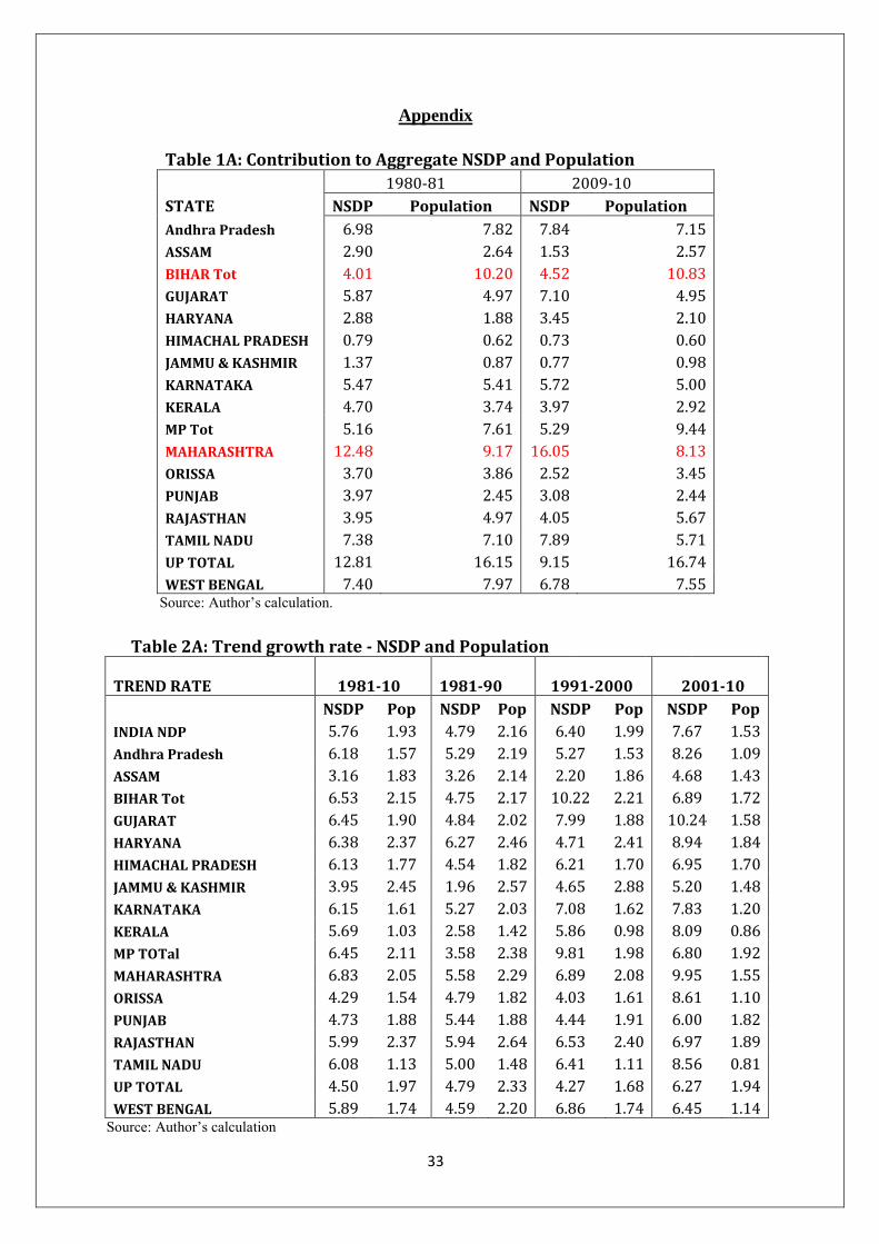
33

Appendix

Table 1A: Contribution to Aggregate NSDP and Population

1980-81 2009-10

STATE NSDP Population NSDP Population

Andhra Pradesh 6.98 7.82 7.84 7.15

ASSAM 2.90 2.64 1.53 2.57

BIHAR Tot 4.01 10.20 4.52 10.83

GUJARAT 5.87 4.97 7.10 4.95

HARYANA 2.88 1.88 3.45 2.10

HIMACHAL PRADESH 0.79 0.62 0.73 0.60

JAMMU & KASHMIR 1.37 0.87 0.77 0.98

KARNATAKA 5.47 5.41 5.72 5.00

KERALA 4.70 3.74 3.97 2.92

MP Tot 5.16 7.61 5.29 9.44

MAHARASHTRA 12.48 9.17 16.05 8.13

ORISSA 3.70 3.86 2.52 3.45

PUNJAB 3.97 2.45 3.08 2.44

RAJASTHAN 3.95 4.97 4.05 5.67

TAMIL NADU 7.38 7.10 7.89 5.71

UP TOTAL 12.81 16.15 9.15 16.74

WEST BENGAL 7.40 7.97 6.78 7.55 Source: Author’s calculation.

Table 2A: Trend growth rate - NSDP and Population

TREND RATE 1981-10 1981-90 1991-2000 2001-10

NSDP Pop NSDP Pop NSDP Pop NSDP Pop

INDIA NDP 5.76 1.93 4.79 2.16 6.40 1.99 7.67 1.53

Andhra Pradesh 6.18 1.57 5.29 2.19 5.27 1.53 8.26 1.09

ASSAM 3.16 1.83 3.26 2.14 2.20 1.86 4.68 1.43

BIHAR Tot 6.53 2.15 4.75 2.17 10.22 2.21 6.89 1.72

GUJARAT 6.45 1.90 4.84 2.02 7.99 1.88 10.24 1.58

HARYANA 6.38 2.37 6.27 2.46 4.71 2.41 8.94 1.84

HIMACHAL PRADESH 6.13 1.77 4.54 1.82 6.21 1.70 6.95 1.70

JAMMU & KASHMIR 3.95 2.45 1.96 2.57 4.65 2.88 5.20 1.48

KARNATAKA 6.15 1.61 5.27 2.03 7.08 1.62 7.83 1.20

KERALA 5.69 1.03 2.58 1.42 5.86 0.98 8.09 0.86

MP TOTal 6.45 2.11 3.58 2.38 9.81 1.98 6.80 1.92

MAHARASHTRA 6.83 2.05 5.58 2.29 6.89 2.08 9.95 1.55

ORISSA 4.29 1.54 4.79 1.82 4.03 1.61 8.61 1.10

PUNJAB 4.73 1.88 5.44 1.88 4.44 1.91 6.00 1.82

RAJASTHAN 5.99 2.37 5.94 2.64 6.53 2.40 6.97 1.89

TAMIL NADU 6.08 1.13 5.00 1.48 6.41 1.11 8.56 0.81

UP TOTAL 4.50 1.97 4.79 2.33 4.27 1.68 6.27 1.94

WEST BENGAL 5.89 1.74 4.59 2.20 6.86 1.74 6.45 1.14 Source: Author’s calculation

34

Table 3A: TREND GROWTH RATES IN PCNSDP TREND RATE 1981-10 1981-90 1991-2000 2001-10

INDIA PCNDP 3.89 2.89 3.90 6.18

Andhra Pradesh 4.54 3.03 3.69 7.09

ASSAM 1.30 1.10 0.33 3.20

BIHAR 4.29 2.53 7.84 5.08

GUJARAT 4.46 2.77 6.00 8.53

HARYANA 3.92 3.72 2.25 6.98

HIMACHAL PRADESH 4.28 2.67 4.43 5.16

JAMMU & KASHMIR 1.46 -0.60 1.72 3.67

KARNATAKA 4.47 3.18 5.38 6.55

KERALA 4.61 1.14 4.83 7.16

MP 4.25 1.17 7.68 4.79

MAHARASHTRA 4.69 3.21 4.71 8.28

ORISSA 2.71 2.92 2.38 7.43

PUNJAB 2.80 3.49 2.48 4.11

RAJASTHAN 3.53 3.22 4.03 4.98

TAMIL NADU 4.89 3.46 5.25 7.69

UP 2.49 2.40 2.55 4.25

WEST BENGAL 4.08 2.33 5.04 5.25 Source: Author’s calculation

Table 4A: Classification of states based on average PCNSDP

State 1981-10 State 1981-90 State 1991-00 State 2001-10

BIHAR 7782.02 BIHAR 4779.40 BIHAR 7628.54 BIHAR 10938.13

UP 12138.48 MP 7526.22 UP 12057.05 UP 15059.61

MP 12493.74 UP 9298.78 ORISSA 12385.35 Assam 17085.53

ORISSA 13924.40 Rajasthan 9915.67 MP 12616.75 MP 17338.27

Rajasthan 14806.43 WB 10651.16 ASSAM 14503.66 ORISSA 18400.95

Assam 14937.67 Orissa 10986.89 Rajasthan 14848.44 Rajasthan 19655.18

WB 16477.33 AP 11254.62 WB 14939.84 J&K 22409.21

AP 18473.77 Karnataka 12361.98 AP 16445.87 WB 23840.98

J&K 19098.92 TN 12978.66 J&K 18155.06 AP 27720.81

Karnataka 20244.15 Assam 13223.82 Karnataka 18730.92 Karnataka 29639.54

Kerala 22494.49 KERALA 13474.84 KERALA 19986.06 HP 33753.51

TN 22584.27 HP 14443.13 HP 20479.77 TN 33954.28

HP 22892.13 GUJARAT 14637.68 TN 20819.86 KERALA 34022.58

Gujarat 23841.99 Maharashtra 16180.50 GUJARAT 22145.09 GUJARAT 34743.20

Maharashtra 27546.82 J&K 16732.47 Maharashtra 25773.93 PUNJAB 35214.51

PUNJAB 27569.67 Haryana 18756.53 HARYANA 25811.53 HARYANA 40610.80

HARYANA 28392.95 PUNJAB 20512.84 PUNJAB 26981.65 Maharashtra 40686.01

India=18340 India=12149.78 India= 16763.3 India= 26106.8

P = LESS THAN 15091.5 P= LESS THAN 11634.5 P=LESS THAN 15823 P= LESS THAN 23821

R= MORE THAN 20588.4 R=MORE THAN 12665 R=MORE THAN 17703 R= MORE THAN 28392.6

35

Note: P= Poor income, R= Rich income state. States with average PCNSDP between poor and rich bandwidth

fall into middle income states.

Table 5A: Classification of states based on trend growth rate

State 1981-10 State 1981-90 State 1991-00 State 2001-10

ASSAM 1.30 J&K -0.60 ASSAM 0.33 ASSAM 3.20

J&K 1.46 ASSAM 1.10 J&K 1.72 J&K 3.67

UP 2.49 KERALA 1.14 HARYANA 2.25 PUNJAB 4.11

ORISSA 2.71 MP 1.17 ORISSA 2.38 UP 4.25

PUNJAB 2.80 WB 2.33 PUNJAB 2.48 MP 4.79

RAJASTHAN 3.53 UP 2.40 UP 2.55 RAJASTHAN 4.98

HARYANA 3.92 Bihar 2.53 AP 3.69 Bihar 5.08

WB 4.08 HP 2.67 RAJASTHAN 4.03 HP 5.16

MP 4.25 GUJARAT 2.77 HP 4.43 WB 5.25

HP 4.28 ORISSA 2.92 Maharashtra 4.71 KARNATAKA 6.55

Bihar 4.29 AP 3.03 KERALA 4.83 HARYANA 6.98

GUJARAT 4.46 KARNATAKA 3.18 WB 5.04 AP 7.09

KARNATAKA 4.47 Maharashtra 3.21 TN 5.25 KERALA 7.16

AP 4.54 RAJASTHAN 3.22 KARNATAKA 5.38 ORISSA 7.43

KERALA 4.61 TN 3.46 GUJARAT 6.00 TN 7.69

Maharashtra 4.69 PUNJAB 3.49 MP 7.68 Maharashtra 8.28

TN 4.89 HARYANA 3.72 Bihar 7.84 GUJARAT 8.53

India=3.89% India=2.89% India= 3.9% India= 6.18%

L = LESS THAN 3.39 L = LESS THAN 2.39 L= LESS THAN 3.40 L = LESS THAN 5.68

H= MORE THAN 4.39 H= MORE THAN 3.39 H= MORE THAN 4.40 H= MORE THAN 6.68 Note: L= Low growth, H= high growth. States with growth rate between low and high growth bandwidth fall

into middle growth state

TABLE : Classification of states as High, Medium and Low Income Regions

Year High Income Medium Income Low Income

1980s Punjab, Haryana,

Maharashtra, Gujarat,

Himachal Pradesh,

Kerala, Assam, J&K

Karnataka, Tamil

Nadu

Bihar, MP, UP,

Rajasthan, West

Bengal, Orissa, Andhra

Pradesh



Himachal Pradesh,

Kerala, Tamil Nadu,

Karnataka, J&K

Andhra Pradesh Bihar, MP, UP,

Rajasthan, West

Bengal, Orissa, Assam



Himachal Pradesh,

Kerala, Tamil Nadu,

Karnataka

West Bengal, Andhra

Pradesh

Bihar, MP, UP,

Rajasthan,J&K, Orissa,

Assam

36

References

Agarwalla. A. (2011). “Estimating the Contribution of Infrastructure in Regional

Productivity Growth in India”, Working Paper No. 2011-05-01, Indian Institute of

Management, Ahmedabad.

Aschauer, D.A. (1989). “Is public expenditure productive?”. Journal of Monetary

Economics (23), pp. 177-200.

Barro, R. (1990). “Government Spending in a Simple Model of Endogenous Growth.”

Journal of Political Economy, 98, October, part II, S103- S125.

Barro, R. and Sala-i-Martin, X. (2004). Economic Growth. 2nd

edition. Boston: MIT

Press.

Boarnet, M.G (1991). “Spillovers and the Location Effects of Public Infrastructure”,

Department of Urban and Regional Planning and Institute of Transport Studies. University

of California , Irvine.’

Bonaglia, F., La Ferrara, E., and Marcellino, M. (2001). “Public capital and economic

performance: Evidence from Italy”. IGIER Working Paper No. 163.

Cadot, O., Röller, L.H., and Stephan, A. (1999). “A political economy model of

infrastructure allocation: An empirical assessment”. CEPR Discussion Paper No. 2336.

Cadot, O., Röller, L.H., and Stephan, A. (2002). “Contribution to productivity or pork

barrel? The two faces of infrastructure investment”. WZB Discussion Paper No. 02-09.

Calderón, C. and Servén, L. (2002). “The output cost of Latin America’s infrastructure

gap”. Central Bank of Chile Working Paper No. 186.

Canning, D. and Bennathan, E. (2000). “The social rate of return on infrastructure

investments”. World Bank Working Paper No. 2390.

Canning, D. and Pedroni, P. (1999). “Infrastructure and long run economic growth”.

Mimeo.

Canning, David, Marianne Fay, and Roberto Perotti. (1994). "Infrastructure and

Growth," in M. Bsaldassarri, M. Paganaetto and E.S. Phelps, eds., International Differences

in Growth Rates. New York: St. Martins Press.

Cashin, P and R. Sahay. (1996). “Internal Migration, Centre-State Grants and Economic

Growth in the States of India”, IMF Staff Papers, Vol.43, No.1, pp123-171

37

Charlot, S and Schmitt, B. (1999). “Public infrastructure and economic growth in France’s

regions”. Paper No.129 for ERSA 39th Congress, Dublin, Ireland.

Demetriades, P.O., and Mamuneas, T.P. (2000). “Intertemporal output and employment

effects of public infrastructure capital: Evidence from 12 OECD economies”. Economic

Journal, (110), pp. 687–712.

Devarajan S., Swaroop, V., and Zou, H.F. (1996). “The composition of public

expenditure and economic growth”. Journal of Monetary Economics, (37), pp. 313-344.

Easterly, W. and Rebelo, S. (1993). “Fiscal policy and economic growth: an empirical

investigation”. Journal of Monetary Economics, (32), pp. 417– 458.

Easterly, William, and Sergio Rebelo. (1994). “Africa’s Growth Tragedy: Policies and

Ethnic Divisions,” World Bank, February 1994.

Economic Intelligence Service. Various years. Centre for Monitoring Indian Economy.

Esfahani, H., and Ramíres, M.T. (2003). “Institutions, infrastructure and economic

growth”. Journal of Development Economics, (70), pp. 443-477.

Everaert, G. and Heylen, F. (2004). “Public capital and long-term labour market

performance in Belgium”. Journal of Policy Modelling, (26), pp. 95–112.

Ghosh,B and De, Prabir. (1998). “Role of Infrastructure in Regional Development: A

Study over the Plan Period”. Economic and Political Weekly Vol. 33, No.47/48 (Nov.21 –

Dec. 4, 1998), pp. 3039 – 3048.

Government of India. Various Years. Basic Road Statistics. Ministry of Transport.

Government of India. Various Years. Statistical Abstract of India. Central Statistical

Organisation, Ministry of Statistica and Programme Implementation.

Gramlich, Edward M. (1994). “Infrastructure Investment: A Review Essay”, Journal of

Economic Literature, 32, pp. 1176-1196.

Gwartney, J., Holcombe, R.G. and Lawson, R. (2004). “Institutions and the impact of

investment on growth”. Paper presented at the Conference of the Association Private

Enterprise Education, APEE, (April), Bahamas.

Handbook of Statistics on Indian Economy. (2009). Reserve Bank of India.

38

Higgins, B and D. Savoie. (1995).“Regional Development Theories and Their

Application”, Transaction Publishers, New Brunswick.

Kurian, N.J., (2000). "Widening Regional Disparities in India – Some Indicators",

Economic and Political Weekly, Vol. XXXV, No. 7, February 12-18.

Lall, V. Somik. (1999). “Role of Public Infrastructure Investments in Regional

Development: Experience of Indian States”, Economic and Political Weekly, Vol. 34, No.

12 (Mar. 20-26, 1999), pp 717-725.

Lucas, Robert E. Jr. (1998). “On the Mechanics of Economic Development”. Journal of

Monetary Economics, XXII, 3-42.

Markusen, A (1994). “Interaction between Regional and Industrial Policies: Evidence from

Four Countries”. Proceedings of the World Bank annual Conference on Development

Economics.

Mathur, A. (2001), “National and Regional Growth Performance in the Indian Economy: A

Sectoral Analysis”, paper presented at National Seminar on Economic Reforms and

Employment in Indian Economy, IAMR.

Nagaraj, R., A. Varoudakis and M. A. Veganzones (2000), “Long-Run Growth Trends

and Convergence Across Indian States”, Journal of International Development, Vol. 12.

Nair, K.R.G. (1982), “Regional Experiences in a Developing Economy”. Wiley Eastern,

New Delhi.

Papola,T,S. and Sahu, P.P.(2012) “Growth and Structure of Employment in India : Long-

Term and Post Reform Performance and the Emerging Challenge” A study prepared as part

of research programme Structural Changes, Industry and Employment in the Indian

Economy. Indian Council of Social Science Research.(2012).

Rao, M. Govinda, R.T. Shand and K.P.Kalirajan. (1993). “Convergence of Incomes

Across Indian States: A Divergent View”, Economic and Political Weekly, March 27, pp

769-778.

Richardson, H. W and P.M. Townroe. (1986). “Regional Policies in Developing

Countries.” In P. Nijkamp (ed.) Handbook of Regional and Urban Economics, North

Holland, Amsterdam.

Romer, P. M. (1990). “Endogenous Technological Change”. Journal of Political Economy

9, 71-102.

Sanchez-Robles, B. (1998). “Infrastructure investment and growth: Some empirical

evidence”. Contemporary Economic Policy, (16), pp. 98-108.

39

Seitz, Helmut and G. Licht. (1992). “The Impact of the Provision of Public Infrastructures

on Regional Development in Germany”, Zentrum for Europaische Wirtschaftsforschung

Gmbh, Discussion paper no. 93-13.

Straub, S and Terada- Hagiwara, A (2010) “Infrastructure and Growth in Developing

Asia”. Asian Development Bank Institute, Economics Working Paper Series No.231,

Tokyo.

Sturm, J.E., Kuper, G.H., and de Haan, J. (1998). “Modelling government investment

and economic growth on a macro level: A review”, in Brakman, S., van Ees, H., and

Kuipers, S.K. (eds.), Market Behaviour and Macroeconomic Modelling. MacMillan Press

Ltd, London, UK.

Sumedha Bajar - cesifo-group.de · Sumedha Bajar I. Introduction Achieving balanced economic growth...

Documents

Transcript of Sumedha Bajar - cesifo-group.de · Sumedha Bajar I. Introduction Achieving balanced economic growth...