Sumca: Simple, Unified, Monte-Carlo Assisted Approachto Second-order Unbiased MSPE Estimation

Jiming Jiang and Mahmoud Torabi

University of California, Davis and University of Manitoba

We propose a simple, unified, Monte-Carlo assisted (Sumca) approach to second-

order unbiased estimation of mean squared prediction error (MSPE) of a small area

predictor. The proposed MSPE estimator is easy to derive, has a simple expression,

and applies to a broad range of predictors that include the traditional empirical best

linear unbiased predictor (EBLUP), empirical best predictor (EBP), and post model

selection EBLUP and EBP as special cases. Furthermore, the leading term of the pro-

posed MSPE estimator is guaranteed positive; the lower-order term corresponds to a

bias correction, which can be evaluated via a Monte-Carlo method. The computational

burden for the Monte-Carlo evaluation is much lesser, compared to other Monte-Carlo

based methods that have been used for producing second-order unbiased MSPE esti-

mators, such as double bootstrap and Monte-Carlo jackknife. The Sumca estimator

also has a nice stability feature. Theoretical and empirical results demonstrate proper-

ties and advantages of the Sumca estimator.

Key Words. approximation, bias correction, Monte Carlo, MSPE, second-order unbi-

asedness, small area estimation

1 Introduction

In recent years there has been substantial interest in small area estimation (SAE) that is

largely driven by practical demands. In policymaking regarding allocation of resources to

subgroups (small areas), or determination of subgroups with specific characteristics (e.g.,

in health and medical studies) in a population, it is desirable that the decisions be made

based on reliable estimates. However, information or data collected from each subgroup

are often inadequate to achieve an acceptable degree of accuracy using the direct survey

method, which computes the estimate solely based on data from the subgroup. For this

reason, demands and interest in research on SAE have kept increasing. Recent reviews on

SAE and related topics can be found, for example, in Pfeffermann (2013), Rao and Molina

(2015), and Jiang (2017, ch. 4).

A major topic in SAE is estimation of mean squared prediction errors (MSPEs) for

predictors of various characteristics of interest associated with the small areas. A standard

practice for the MSPE estimation in the current SAE literature is to produce a second-

order unbiased MSPE estimator, that is, the order of bias of the MSPE estimator is o(m−1),

where m is the total number of small areas from which data are collected (see Section 6

for discussion regarding other aspects of the MSPE estimation). For the most part, there

have been two approaches for producing a second-order unbiased MSPE estimator. The

first is the Prasad-Rao linearization method (Prasad and Rao 1990). The approach uses

Taylor series expansion to obtain a second-order approximation to the MSPE, then corrects

the bias, again to the second-order, to produce an MSPE estimator whose bias is o(m−1).

Various extensions of the Prasad-Rao method have been developed; see, for example, Datta

and Lahiri (2000), Jiang and Lahiri (2001), Das, Jiang and Rao (2004), and Datta, Rao and

Smith (2005). Although the method often leads to an analytic expression of the MSPE

estimator, the derivation is tedious, and the final expression is likely to be complicated.

The linearization method also does not apply to situations where a non-differentiable oper-

ation is involved in obtaining the predictor, such as model selection (e.g., Jiang, Lahiri and

Nguyen 2018) and shrinkage estimation (e.g., Tibshirani 1996).

The second approach to second-order unbiased MSPE estimation is resampling meth-

ods. Jiang, Lahiri and Wan (2002; hereafter, JLW) proposed a jackknife method to estimate

the MSPE of an empirical best predictor (EBP) of a mixed effect associated with the small

areas. The method avoids tedious derivations, and is “one formula for all”. On the other

2

hand, there are certain restrictions on the class of predictors to which JLW applies. Namely,

for the JLW to be applicable to the empirical best linear unbiased predictor (EBLUP),

widely used in SAE, a posterior linearity condition needs to be satisfied. This is not the

case, for example, if the random effects involved in a linear mixed model (LMM) for SAE

are not normally distributed. Also, JLW does not apply to a predictor that is obtained post

model selection. In order to solve the latter problem, Jiang et al. (2018) proposed a Monte-

Carlo jackknife method (McJack). The method leads to a second-order unbiased MSPE

estimator in situations like post-model selection (PMS); however, it is computationally in-

tensive. Another resampling-based approach is double bootstrapping (DB; Hall and Maiti

2006a,b). Although DB is capable of producing a second-order unbiased MSPE estimator,

it is, perhaps, computationally even more intensive than the McJack.

The method to be proposed in this paper may be viewed as a hybrid of the linearization

and resampling methods, by combining the best part of each method. We use a simple,

analytic approach to obtain the leading term of our MSPE estimator, and a Monte-Carlo

method to take care of a remaining, lower-order term. The computational cost for the

Monte-Carlo part is much less compared to McJack and DB in order to achieve second-

order unbiasedness. More importantly, the method provides a unified and conceptually

easy solution to a hard problem, that is, obtaining a second-order unbiased MSPE estimator

for a possibly complicated predictor.

A heuristic derivation of the MSPE estimator, called Sumca (which is an abbreviation

of simple, unified, Monte-Carlo assisted) estimator, is given in the next section, which is

followed by rigorous theoretical justification. In Section 3, we consider the special case

of PMS predictors. In Section 4, we illustrate the Sumca method with a few examples.

In Section 5, we study performance of the Sumca estimator, and compare it with popular

existing estimators via Monte-Carlo simulation. A concluding remark is offered in Section

6. Technical and additional empirical results, including real-data applications, are provided

3

in the Supplementary Material.

2 Derivation and justification

We begin with a heuristic derivation of the proposed MSPE estimator, followed by

rigorous justification. The essential idea of the derivation is the same as that used in the

seminal paper of Prasad and Rao (1990) and subsequent work on linearization methods as

well as resampling methods for higher order unbiasedness (e.g., Jiang et al. 2002, Hall

and Maiti 2006a). Namely, for a sufficiently smooth function g(ψ) and under regularity

conditions, the bias of g(ψ) for estimating g(ψ) is O(m−1) for a root-n consistent (and

asymptotically normal) estimator ψ. If one writes the bias as c(ψ)/m + o(m−1), where

c(ψ) is another smooth function, one can, again, approximate c(ψ) by c(ψ) to obtain a

bias-corrected estimator whose bias is o(m−1). The latter type of bias expansion can also

be found, for example, in the context of jackknife (e.g., Shao and Tu 1995, p. 5).

Let θ denote a mixed effect, that is, a (possibly nonlinear) function of fixed and random

effects that are associated with a mixed effects model (e.g., Jiang 2007). Let θ be a predictor

of θ, that is, a function of the observed data, y. Here, θ may be a traditional predictor like

EBLUP, or EBP, or something more complicated like the PMS EBLUP or EBP, to which

the standard methods such as Prasad-Rao and JLW do not apply to obtain a second-order

unbiased MSPE estimator. The MSPE of θ can be expressed as

MSPE = E(θ − θ)2 = E[E{(θ − θ)2|y}

]. (1)

Suppose that the underlying distribution of y depends on a vector of unknown parameters,

ψ. Then, the conditional expectation inside the expectation on the right side of (1) is a

function of y and ψ, which can be written as

a(y, ψ) = E{(θ − θ)2|y} = θ2 − 2θh1(y, ψ) + h2(y, ψ), (2)

4

where hj(y, ψ) = E(θj|y), j = 1, 2. If we replace the ψ in (2) by ψ, a root-n consistent

and asymptotically normal estimator of ψ, then under regularity conditions such as differ-

entiability and dominatedness (e.g., Jiang 2010, p. 32), the result is a first-order unbiased

estimator of the MSPE, that is,

E{a(y, ψ)− a(y, ψ)} = O(m−1). (3)

On the other hand, both MSPE = E{a(y, ψ)} [by (1), (2)] and E{a(y, ψ)} are functions of

ψ, denoted by b(ψ) and c(ψ), respectively. By (3), we have d(ψ) = b(ψ)−c(ψ) = O(m−1);

thus, if we replace, again, ψ by ψ in d(ψ), the difference would be a lower-order term,

d(ψ)− d(ψ) = oP(m−1). (4)

Now consider the estimator

MSPE = a(y, ψ) + b(ψ)− c(ψ). (5)

One would have, by (1)–(5), E(MSPE) = E{a(y, ψ)}+E{a(y, ψ)−a(y, ψ)}+E{d(ψ)} =

MSPE+E{d(ψ)−d(ψ)} = MSPE+o(m−1). Essentially, this one-line, heuristic derivation

shows the second-order unbiasedness of the proposed MSPE estimator, (5), provided that

it can be justified and the terms involved can be evaluated (see below).

It should be noted that, strictly speaking, virtually all the subjects we deal with, such as

a(y, ψ), d(ψ), depend on m and possibly other quantities, such as ni, the sample size for

the ith small area, which may increase withm. In fact, in many small-area applications, the

ni’s are random outcomes, although extension to such a case is relatively straightforward

(e.g. Jiang 2001); thus, for the sake of simplicity, the ni are considered as non-random

in this paper. Also, dependency of different quantities on m is suppressed for notational

simplicity [e.g., d(ψ) instead of dm(ψ)]. The limiting process is m → ∞, with other

quantities considered as functions of m.

5

Remark 1. Another seeming advantage of the proposed MSPE estimator is that the

leading term, a(y, ψ), is guaranteed positive. This can be seen from the definition, that is,

a(y, ψ) = E{(θ − θ)2|y}∣∣∣ψ=ψ

. (6)

See, for example, Jiang et al. (2018, sec. 1) for discussion on importance, and difficulty, of

achieving the “double goal”, that is, second-order unbiasedness and positivity at the same

time, for an MSPE estimator. Typically, the leading term, (6), is O(1), while the remaining

term, b(ψ) − c(ψ), is O(m−1), assuming that ψ is a root-n consistent and asymptotically

normal estimator. As a result, the MSPE estimator (5), as well as the Sumca estimator (see

below), are positive with probability tending to one as m increases.

A special form of the leading term, a(y, ψ), deserves attention. We can write

a(y, ψ) = {θ − E(θ|y)}2 + var(θ|y). (7)

When θ is the EBP, defined as

θ = E(θ|y)|ψ=ψ, (8)

the first term on the right side of (7) vanishes when ψ is replaced by ψ, hence

a(y, ψ) = var(θ|y)|ψ=ψ. (9)

Expression (9) is especially attractive under a general linear mixed model, defined as

y = Xβ + Zv + e, (10)

where X and Z are known matrices, v is a vector of random effects, and e is a vector of

errors. Suppose that v and e are independent with v ∼ N(0, G) and e ∼ N(0, R), where

the covariance matrices G and R depend on a vector γ of dispersion parameters. Now

suppose that θ is a linear mixed effect with the expression θ = a′β + b′v, where a, b are

6

known vectors. Then, by the properties of multivariate normal distribution, var(θ|y) does

not depend on y; in other words, var(θ|y) is a function of γ only (which is part of ψ). Write

var(θ|y) = V (γ). Then, by (9), we have

a(y, ψ) = V (γ). (11)

An advantage of expression (11) is stability, because, typically, the variance of a smooth

function of γ is O(m−1). In this case, the variance of the leading term of the MSPE esti-

mator, (5), is O(m−1). The stability of our proposed MSPE estimator (see below) is also

demonstrated numerically in our simulation studies in Section 5 as well as in the Supple-

mentary Material. See further discussion in Section 6.

The lower-order term in (5), b(ψ)−c(ψ), corresponds to a bias correction to the leading

term. Deriving an analytic form of this term, up to the order o(m−1), may require tedious al-

gebra. To overcome this difficulty, we approximate this term using a Monte-Carlo method.

Let Pψ denote the distribution of y with ψ being the true parameter vector. Given ψ, one

can generate y under Pψ. Let y[k] denote y generated under the kth Monte-Carlo sample,

k = 1, . . . , K. Then, we have

b(ψ)− c(ψ) ≈ 1

K

K∑k=1

{a(y[k], ψ)− a(y[k], ψ[k])

}, (12)

where ψ[k] denotes ψ based on y[k]. Write the right side of (12) as dK(ψ) (note that y[k], k =

1, . . . , K also depend on ψ). Then, a Monte-Carlo assisted MSPE estimator, which we call

Sumca estimator, is given by

MSPEK = a(y, ψ) + dK(ψ) = a(y, ψ) +1

K

K∑k=1

{a(y[k], ψ)− a(y[k], ψ[k])

}, (13)

where y[k], k = 1, . . . , K are generated as above with ψ = ψ, and ψ[k] is, again, the estima-

tor of ψ based on y[k]. It can be shown (see below) that the Sumca estimator is second-order

unbiased with respect to the joint distribution of the data and Monte-Carlo sampling.

7

Remark 2. Sumca is computationally much less intensive than McJack (Jiang et al.

2018). This is because McJack requires m2/K → 0, while Sumca does not have such a

restriction. In fact, as far as second-order unbiasedness is concerned, there is no restriction

onK for Sumca; however, it is typically required thatK is large enough so that the variance

of the second term on the right side of (13) is of lower order than that of the first term. For

example, if var{a(y, ψ)} = O(1), all that is required is K → ∞. In Section 6, it is

recommended that K = m in standard situations. Also, for McJack, one needs to evaluate

m+ 1 terms using Monte-Carlo, while for Sumca there is only one term that needs Monte-

Carlo. Overall, the amount of computation for Sumca is somewhere between 1/m3 to 1/m2

of that for McJack, which could be a highly significant saving if m is relatively large.

A rigorous justification is given below, with technical details deferred to the Supple-

ment. We first state some general conditions under which the second-order unbiasedness

of the MSPE estimator (5) holds. Let ψ be the estimator of ψ, and Ψ the parameter space

for ψ. Following Jiang et al. (2002) and Das, Jiang and Rao (2004), we consider a sequence

of subsets, Ψm ⊂ Ψ, such that Ψm is compact and lies strictly in Ψo, the interior of Ψ, and

approaches Ψ as m → ∞ in the sense that Ψm ⊂ Ψm+1 for any m ≥ 1, and any point

in Ψo will be covered by Ψm for sufficiently large m. A truncated estimator (e.g., Das et

al. 2004) is defined as ψ = ψo if ψo ∈ Ψm, and ψ = ψ∗ otherwise, where ψ∗ is a known

vector that belongs to Ψm. Note that, if the true ψ ∈ Ψo and ψo is a consistent estimator,

then we have with probability tending to one that ψ = ψo; in other words, asymptotically,

the truncated estimator is equal to the original estimator. In practice, the truncation does

not change the value of the estimator (see a note in the first paragraph of the Supplement).

Theorem 1. The MSPE estimator given by (5) is second-order unbiased, that is,

E(MSPE) = MSPE + o(m−1) provided that the following hold:

A1. E(θ2|y) is finite almost surely, and the expectations E{a(y, ψ)} and E{a(y, ψ)} exist.

A2. ψ ∈ Ψm for large m, and we have the following expansion, d(ψ) = m−1q(ψ) + r(ψ)

8

for some q(·), r(·) satisfying supψ∈Ψm|r(ψ)| = o(m−1) and E{|q(ψ)− q(ψ)|} = o(1).

Proof: We need to make the heuristic derivation below (5) for the second-order unbi-

asedness rigorous. Given A1, we just have to show that E{d(ψ)− d(ψ)} = o(m−1). Note

that, by A2, we have d(ψ)− d(ψ) = m−1{q(ψ)− q(ψ)}+ r(ψ)− r(ψ). Note that ψ ∈ Ψm

for large m by A2; also ψ ∈ Ψm by the definition of the truncated estimator. Thus, we have

|r(ψ) − r(ψ)| ≤ 2 supψ∈Ψm|r(ψ)| for large m, and the latter is o(m−1) by A2. It follows

that |E{d(ψ)− d(ψ)}| ≤ m−1E(|q(ψ)− q(ψ)|) + o(m−1) = o(m−1).

Theorem A.1 in the Supplementary Material provides verifiable technical conditions

under which the assumptions of Theorem 1, especially A2, hold. To provide some illustra-

tion on what kinds of situations where one may expect these technical conditions to hold,

consider the following examples below. The first example is the Fay-Herriot model of Sec-

tion 4.1 below. The mixed effect of interest is the small area mean, θi = x′iβ + vi, where

vi ∼ N(0, A) (1 ≤ i ≤ m). Suppose that the Prasad-Rao estimator of A is used. Then, the

technical conditions of Theorem A.1 are satisfied provided that there are positive constants

b, B such that b ≤ Di ≤ B, 1 ≤ i ≤ m, and lim infm→∞ λmin(m−1∑m

i=1 xix′i) > 0, where

λmin denotes the smallest eigenvalue. The second example is a special case of the mixed

logistic model of Section 4.3 in the sequel with x′ijβ = β. The mixed effect of interest is

the conditional probability, θi = P(yij = 1|vi). Suppose that the MLE of (β,A) is used.

Then, the technical conditions of Theorem A.1 are satisfied provided that ni, 1 ≤ i ≤ m

are bounded and lim infm→∞{(logm)Lpm} > 0 for some constant L > 0, where pm is the

proportion of ni, 1 ≤ i ≤ m satisfying ni > 1.

Now let us consider the Sumca estimator (13). We assume that the Monte-Carlo (MC)

samples, under ψ, are generated by first generating some standard [e.g., N(0, 1)] random

variables, say, ξ, whose distribution does not depend on ψ. We then combine ξ with ψ to

produce the MC samples under ψ. A precise statement of this assumption is the following:

For any given ψ, the summand in (12), a(y[k], ψ) − a(y[k], ψ[k]), where ψ[k] is ψ based on

9

y[k], can be expressed as a function of ξ[k] and ψ, say, ∆(ξ[k], ψ), where ξ[k], 1 ≤ k ≤ K are

i.i.d. whose distribution does not depend on ψ, and are independent with the data y. This

implies that the summands of (13) can be expressed as ∆(ξ[k], ψ), 1 ≤ k ≤ K with the same

ξ[k], 1 ≤ k ≤ K. For example, under the Fay-Herriot model (see Sections 4.1, 5.1 below),

the yi’s are generated by first generating the ξi’s and ηi’s, which are independent N(0, 1),

and then letting yi = x′iβ +√Aξi +

√Diηi, where ψ = (β′, A)′. More generally, if the

distributions of the random effects and errors are scale families, then the above assumption

about the MC samples holds. As an example beyond the scale family, suppose that, in the

Fay-Herriot model, the cumulative distribution function (cdf) of vi is Fψ(·) and that of ei

is Gi,ψ(·) such that the cdf’s are continuous. Then, given ψ, vi and ei can be generated by

F−1ψ (Ui), G−1

i,ψ(Vi), where Ui and Vi are independent Uniform[0, 1] random variables, and

F−1ψ (·), G−1

i,ψ(·) are the inverse distribution functions (e.g., Jiang 2010, Theorem 7.1).

Theorem 2. Suppose that the MC samples are generated as described above, where ξ is

independent with y, the original data. Then, under the assumptions of Theorem 1, we have

E(MSPEK) = MSPE + o(m−1), (14)

where the expectation is with respect to the joint distribution of y and ξ.

The proof of Theorem 2 is given in the Supplementary Material.

3 Post model selection predictor

In some applications, model selection is involved prior to computing the predictor. Let

θM be the predictor of θ computed under model M . The PMS predictor of θ is defined as

θP = θM , where the subscript P stands for PMS, and M is the model selected by applying

some model selection procedure, such as the information criteria or the fence methods (e.g.,

Jiang et al. 2008; Muller, Scealy and Welsh 2013).

10

We restrict our attention to consistent model selection procedures. Some restriction on

the convergence rate of the model selection consistency will be imposed. Furthermore,

we follow the classical setting of consistency in model selection, in which the space of

candidate models, M, is finite, and there is a unique optimal model, Mo ∈M, that is, a true

model that cannot be simplified. For example, in regression variable selection, suppose

that the true (predictor) variables are a subset of the candidate variables. Then, any subset

of candidate variables that include the true variables corresponds to a true model, with the

understanding that the regression coefficients of the variables other than the true variables

are zero. It is clear that the optimal model in this case corresponds to the subset that

contains only the true variables. Mathematically, the precise definition of Mo, is the limit

of convergence of the model selection procedure, M , that we deal with in Theorem 3 and

Theorem 4 so that the conditions of those theorems are satisfied. We also assume that

there is a full model, Mf , in M so that every candidate model is a sub-model of Mf . For

example, in the case of regression variable selection, Mf is the subset of all of the candidate

variables. It should also be made clear that these candidate models, M, including Mo and

Mf , as well as the parameter spaces under these models (see below), are finite-dimensional,

whose dimensions do not change as the sample size increases. Note that, under the above

assumptions, Mf is, at least, a true model; however, it may not be the most efficient one

in that it may allow further simplification, for example, by dropping the variables whose

coefficients are zero in the regression variable selection problem. Finding the most efficient

true model, that is, Mo, is often the purpose of model selection.

For M ∈ M, let ψM denote the vector of parameters under M , ψM the estimator of

ψM , and θM the predictor of θ, the mixed effect of interest, derived under M . If M is

given, then ψM and θM are the ones discussed in the previous sections. The only additional

step, here, is the process of model selection prior to computing ψM and θM . Let M denote

the selected model via the model selection procedure. Then, the PMS estimator of the

11

parameters, under the selected model, is ψP = ψM ; the PMS predictor of θ is θP = θM .

A measure of uncertainty for θP is, again, its MSPE defined as MSPE(θP) = E(θP − θ)2.

Note that the MSPE is a measure of overall uncertainty in θP, which includes the uncertain

in model selection, in parameter estimation given the selected model, and prediction under

the selected model. It is not necessarily true that the overall uncertainty is larger than

uncertainty in prediction under a fixed model. For example, if a simpler model is selected,

it may help to reduce the uncertainty in parameter estimation; on the other hand, if a more

complex model is selected, it may help to reduce the prediction error. The bottom line is

that the MSPE of θP is more complex than that of θM under a fixed M .

The Sumca method can be used to estimate the MSPE of θP. First note that, in (2),

E stands for the true conditional expectation. Following Jiang et al. (2015), in a PMS

situation, the conditional expectations in (2) is evaluated under Mf , which is a true model,

and ψf ≡ ψMf, the vector of true parameters under Mf , if the latter is given. With this

understanding, all of the derivations in Section 2 carry through with ψ replaced by ψf , and

ψ replaced by ψf ≡ ψMf, the estimator of ψf . Note that there is no need to change the

notation E, because expectation under Mf (and ψf) is the true expectation.

Two facts need to be noted. First, let ψo ≡ ψMo denote the true parameter vector under

Mo. Then, becauseMf is also a true model, any expectation underMo and ψo is the same as

that under Mf and ψf . As a result, any function of ψo that is obtained via taking expectation

(even repeatedly) can be expressed as a function of ψf by the same operation. As far as this

paper is concerned, only such functions are involved.

Second, let Ef denote expectation, or conditional expectation, underMf and the true ψf .

We assume that the mixed effect of interest, θ, is the same under any true model and true

parameters. For example, if θ = x′iβ + vi, the value of θ does not change if one adds, or

drops, zero components to β (and adjusts xi correspondingly). Then, the PMS version of

12

(2) can be written as

a(y, ψf) = θ2P − 2θPh1(y, ψf) + h2(y, ψf), (15)

where hj(y, ψf) = Ef(θj|y), j = 1, 2. Let ao(y, ψf), aM(y, ψf) be (15) with θP replaced by

θo ≡ θMo , θM , respectively. We have with the following obvious equations:

a(y, ψf)− ao(y, ψf) =∑M 6=Mo

{aM(y, ψf)− ao(y, ψf)}1(M=M), (16)

aM(y, ψf)− ao(y, ψf) = θ2M − θ2

o − 2h1(y, ψf)(θM − θo), (17)

using (15) for (17). Let bo(ψf) = Ef{ao(y, ψf)} and co(ψf) = Ef{ao(y, ψf)}. An al-

ternative expression of the MSPE estimator, (5) (note that now ψ = ψf), that is useful

for the theoretical derivation (but not for computing purposes) is the following: Define

MSPE1 = ao(y, ψf) + bo(ψf)− co(ψf); then, we have

MSPE− MSPE1 = 2Ef [{h1(y, ψf)− h1(y, ψf)}(θP − θo)1(M 6=Mo)]∣∣∣ψf=ψf

. (18)

Note that MSPE1 looks quite similar to the MSPE in (5), with one difference: Typically,

θ involves a parameter estimator. In (5), the parameter estimator in θ is the same as that

involved elsewhere, that is, ψ. In MSPE1, the parameter estimator involved in θo is ψo;

elsewhere it is ψf . The most important thing is that there is no model selection involved

in MSPE1 so that its second-order unbiasedness can be proved similarly. The remaining

term, that is, the right side of (18), is negligible as long as M has good consistency property,

which is made precise by condition (iii) in Theorem 3 below.

We can now apply Theorem 1 to the current PMS case. Note that MSPE is now (5)

with ψ replaced by ψf . For a random variable ξ, define ‖ξ‖2 = {E(ξ2)}1/2. Following

Jiang et al. (2002) (also Das et al. 2004), to ensure the existence of the MSPE we consider

a truncated version of ψf . Let Ψf,m be a compact subspace of Ψf , the parameter space of

ψf , which is expanding as m increases (for example, Ψf,m = {ψf : |ψf | ≤ bm}, where | · |

13

denotes the Euclidean norm and bm → ∞ as m → ∞). Note that such a truncation is

only used in a (rigorous) theoretical argument; there is no need to truncate an estimator in

practice. For example, one can change the bm in the definition of Ψf,m by cbm, where c is

any positive constant, and the same argument goes through; on the other hand, it may be

argued that the ψf obtained from the real data satisfies ψf ∈ Ψf,m for some constant c.

Theorem 3. Suppose that the conditions of Theorem 1 hold with ψ replaced by ψf .

Furthermore, suppose that the following hold: (i) supψf∈Ψf,m‖h1(y, ψf) − h1(y, ψf)‖2 ≤

cmδ for some constant c, δ > 0; (ii) ‖θo− θ‖2 = O(mδ); and (iii) ‖θP− θo‖2 = o(m−1−δ).

Then, we have E(MSPE) = MSPE + o(m−1). Define ψf as ψ∗f , where ψ∗f is a known

vector in Ψf,m, if ψf /∈ Ψf,m.

Note that condition (iii) is related to the convergence rate of P(M = Mo) going to one,

or P(M 6= Mo) going to zero. To see this, suppose that θo, θP satisfy ‖θP− θo‖4 = O(mδ),

where ‖ξ‖4 = {E(ξ4)}1/4, then by the Cauchy-Schwarz inequality we have

E(θP − θo)2 = E{(θP − θo)21(M 6=Mo)} ≤ O(m2δ)P(M 6= Mo)1/2.

Thus, provided that P(M 6= Mo) = o(m−4−8δ), the above inequality implies that E(θP −

θo)2 = o(m−2−2δ)), hence ‖θP − θo‖2 = o(m−1−δ). It is know that, in model selection, the

convergence rate of P(M 6= Mo)→ 0 can be at the exponential rate, which is much faster

than m−λ for any λ > 0 (see Section A.1.4 of the Supplementary Material for an example).

The proof of Theorem 3 is given in the Supplementary Material.

Furthermore, Theorem A.1 in the Supplementary Material can be extended to the PMS

case (see Theorem 5 of Jiang and Torabi 2019).

The next result is a PMS version of Theorem 2. Here, the Sumca estimator, MSPEK ,

is given by (13) with ψ replaced by ψf (and ψ by ψf).

Theorem 4. Suppose that the MC samples are generated as described above Theorem

2, where ξ is independent with y. Then (14) holds under the assumption of Theorem 3,

14

where the expectation in (14) is with respect to the joint distribution of y and ξ.

The proof of Theorem 4 is similar to that of Theorem 2, and therefore omitted.

4 Examples

In this section, we demonstrate the Sumca estimator with a few examples. The examples

include a popular area-level SAE model, a situation of PMS SAE, and a mixed logistic

model used for estimating small area proportions.

4.1 Fay-Herriot model

A widely used SAE model is the Fay-Herriot model (Fay and Herriot 1979). The model

can be expressed in terms of a linear mixed model:

yi = x′iβ + vi + ei, i = 1, . . . ,m, (19)

where yi is a direct estimator from the ith area, xi is a vector of known covariate, β is a

vector of unknown fixed effects, vi is an area-specific random effect, and ei is a sampling

error. It is assumed that vi, ei, 1 ≤ i ≤ m are independent with vi ∼ N(0, A) and ei ∼

N(0, Di), where A is an unknown variance but Di is assumed known, 1 ≤ i ≤ m. Here,

the vector of unknown parameters involved in the model is ψ = (β′, A)′. As noted earlier

(see the paragraph following the proof of Theorem 1), the technical conditions of Theorem

A.1 in the Supplement, under the Fay-Herriot model, are satisfied provided that the Di’s

are bounded and bounded away from zero, and lim infm→∞ λmin(m−1∑m

i=1 xix′i) > 0.

Suppose that we are interested in estimating the small area mean, θi = x′iβ + vi, for

each small area i, using the EBP. This is a special case of (10), thus, by (9), we have

ai(y, ψ) = var(θi|y)|ψ=ψ =ADi

A+Di

. (20)

15

The Sumca estimator, (13), is thus given by

MSPEi,K =ADi

A+Di

+1

K

K∑k=1

{ai(y[k], ψ)− ai(y[k], ψ[k])

}. (21)

To be more specific, let us consider the Prasad-Rao estimator of A (Prasad and Rao 1990),

given by A = (m − p)−1{y′PX⊥y − tr(PX⊥D)}, where p = rank(X), y = (yi)1≤i≤m,

PX⊥ = Im − PX , PX = X(X ′X)−1X ′ for X = (x′i)1≤i≤m, and D = diag(D1, . . . , Dm).

Given A, the estimator of β is given by β = β(A), where β(A) = (X ′V −1X)−1X ′V −1y

with V = AIm + D. For this particular EBP, Prasad and Rao (1990) showed that the

following Prasad-Rao MSPE estimator for θi is second-order unbiased:

MSPEi,PR =ADi

A+Di

+

(Di

A+Di

)2

x′i

(m∑j=1

xjx′j

A+Dj

)−1

xi

+4D2

i

(A+Di)3m2

m∑j=1

(A+Dj)2. (22)

Comparing (21) with (22), it is clear that the two estimators have the same leading O(1)

term, ADi/(A + Di); the only difference is the remaining lower-order term, which corre-

sponds to a bias correction. Prasad and Rao (1990) used an analytic bias correction while

Sumca uses a Monte-Carlo bias correction. It can be shown that, in this case, we have

ai(y[k], ψ)− ai(y[k], ψ[k]) = Di

(A

A+Di

−A[k]

A[k] +Di

)

+

{(A[k]

A[k] +Di

− A

A+Di

)y[k],i +Dix

′i

(β[k]

A[k] +Di

− β

A+Di

)}2

, (23)

where y[k],i is the ith component of y[k], and ψ[k] = (β′[k], A[k])′.

Another existing approach to second-order unbiased MSPE estimation is double (para-

metric) bootstrap (DB; Hall and Maiti 2006b). Because it is computationally intensive, in

the simulation study, later in Section 5.1, we compare the DB approach with PR and Sumca

in the case of relatively small m. To obtain the DB estimator, we generate the bootstrap

16

data under (19) with β, A as the true parameters. The small area means for the bootstrap

data are defined accordingly. We then obtain the parameter estimates and small area mean

predictors based on the bootstrapped data. This leads to the first-phase (or single) boot-

strapped MSPE, with the first-phase bootstrap sample size B1. It is known (e.g., Hall and

Maiti 2006a) that the first-phase bootstrapped MSPE is only first-order unbiased. Thus,

in the next step, we draw a second-phase bootstrap sample from a given bootstrap sample

using the bootstrapped model parameters given above. Proceeding as above to obtain the

second-phase bootstrapped MSPE, with the second-phase bootstrap sample size B2. Due

to the computational cost, it is suggested (Hall and Maiti 2006a, b) that B1 is moderately

large and B2 is smaller than B1. Hall and Maiti (2006b) further suggests two nonnega-

tive modifications of the second-phase bootstrapped MSPE. These are the final DB MSPE

estimators, denoted by MSPEi,Boot1 and MSPEi,Boot2, respectively.

4.2 Area-level model with model selection

Datta, Hall and Mandal (2011; hereafter, DHM) proposed a method of model selection

by testing for the presence of the area-specific random effects, vi, in the Fay-Herriot model

(19). Once again, consider the Prasad-Rao estimator of A given below (21). Then, DHM is

equivalent to testing the null hypothesis H0 : A = 0. The test statistic, T =∑m

i=1D−1i (yi−

x′iβ)2, where β = β(0) [defined above (22)], has a χ2m−p distribution under H0. If H0 is

rejected, the EBLUP is used to estimate the small area mean θi; if H0 is accepted, the

estimator θi = x′iβ is used to estimate θi, where β = (X ′D−1X)−1X ′D−1y. Note that, the

combined predictor, θi, is different from the traditional EBLUP; namely, we have

θi =

A(A+Di)−1yi +Di(A+Di)

−1x′iβ, if T > χ2m−p(1− α),

x′iβ, if T ≤ χ2m−p(1− α),

(24)

17

where α is the level of significance. As for the MSPE estimator corresponding to (24),

DHM proposed the following:

MSPEi,DHM = (22) if T > χ2m−p(1− α), and x′i(X

′D−1X)−1xi otherwise. (25)

On the other hand, our Sumca approach applies to any kind of predictor, thus, in par-

ticular, to the predictor (24). The corresponding Sumca estimator is given by (13), where

β, A are the same as in (24) (note that these are consistent estimators of β,A, respectively,

regardless of the null hypothesis). Note that (9) no longer holds in this case, because θi is

not the EBP. In fact, by the right side of (7), we have

ai(y, ψ) =ADi

A+Di

+

(θi −

A

A+Di

yi −Di

A+Di

x′iβ

)2

, (26)

ai(y[k], ψ)− ai(y[k], ψ[k])

= Di

(A

A+Di

−A[k]

A[k] +Di

)+

(θi −

A

A+Di

y[k],i −Di

A+Di

x′iβ

)2

−

(θi −

A[k]

A[k] +Di

y[k],i −Di

A[k] +Di

x′iβ[k]

)2

. (27)

4.3 A mixed logistic model

Jiang and Lahiri (2001) considered the following mixed logistic model for SAE with

binary data. Suppose that, given the area-specific random effects, v1, . . . , vm, binary re-

sponses yij, i = 1, . . . ,m, j = 1, . . . , ni are conditionally independent such that P(yij =

1|v) = pij with logit(pij) = x′ijβ + vi, where v = (vi)1≤i≤m, xij is a vector of known

covariates, and β is a vector of unknown fixed effects. Furthermore, it is assumed that

v1, . . . , vm are independent and distributed as N(0, A), where A is an unknown variance.

For simplicity, consider the case that xij is at area level, that is, xij = xi. The mixed effect

of interest is the conditional probability, θi = h(x′iβ + vi), where h(u) = eu/(1 + eu). As

noted earlier (see the paragraph following the proof of Theorem 1), for the special case of

18

the mixed logistic model with x′iβ = β, the technical conditions of Theorem A.1 in the Sup-

plement are satisfied provided that the ni’s are bounded and lim infm→∞{(logm)Lpm} > 0

for some L > 0, where pm = m−1#{1 ≤ i ≤ m : ni > 1}.

It is easy to show that f(v|y) =∏m

i=1 f(vi|yi), where yi = (yij)1≤j≤niand, with a little

abuse of the notation, f(ξ|η) denotes the conditional pdf of ξ given η. It follows that

hi,s(y, ψ) = E(θsi |y) =

∫{h(x′iβ + vi)}sfβ(yi|vi)fA(vi)dvi∫

fβ(yi|vi)fA(vi)dvi, s = 1, 2, (28)

where fβ(yi|vi) = exp{yi·(x

′iβ + vi)− ni log(1 + ex

′iβ+vi)

}denote the conditional pmf

of yi given vi, with yi· =∑ni

j=1 yij , ψ = (β′, A)′, and fA(·) denotes the pdf of N(0, A).

Expressions (28) involve some one-dimensional integrals, which can be evaluated numer-

ically [e.g., using the R function integrate()]. Given the expressions (28), the EBP of θi is

given by θi = hi,1(y, ψ), where ψ is the maximum likelihood estimator (MLE) of ψ, which

can be computed numerically by fitting the mixed logistic model which is a special case of

the generalized linear mixed models (GLMMs; e.g., Jiang 2007).

Our Sumca estimator also applies to this case. Note that, because θi is the EBP based

on the same ψ, the simplified expression (9) holds, leading to ai(y, ψ) = hi,2(y, ψ) − θ2i ,

ai(y[k], ψ[k]) = hi,2(y[k], ψ[k]) − θ2i,[k], where θi,[k] = hi,1(y[k], ψ[k]); however, there is no

simplification for ai(y[k], ψ).

As a comparison, Jiang et al. (2002; JLW) proposed a jackknife method for estimating

the MSPE, which can be expressed as

MSPEi,JLW = Bi(ψ)− m− 1

m

m∑i′=1

{Bi(ψ−i′)−Bi(ψ)}+m− 1

m

m∑i′=1

(θi,−i′ − θi)2. (29)

In (29), Bi(ψ) is the MSPE of the BP, θi = hi,1(y, ψ), where ψ is the true parameter vector.

Note that hi,s(y, ψ) depends on y only through yi·, therefore can be written as hi,s(yi·, ψ),

s = 1, 2. Furthermore, given vi, yi· is distributed as Binomial(ni, θi). It can be shown that

Bi(ψ) =

ni∑k=1

Cnik

[hi,2(k, ψ)− {hi,1(k, ψ)}2

]E{θki (1− θi)ni−k}, (30)

19

where Cnk is the binomial coefficient of n choose k, θi = h(x′iβ + vi), and the expectation

is taken with respect to vi ∼ N(0, A). Again, Bi(ψ) can be evaluated via numerical inte-

gration. The ψ−i′ in (29) is obtained the same way as ψ but with the i′th cluster of the data,

(yi′ , xi′), deleted; and θi,−i′ = hi,1(yi·, ψ−i′).

Another alternative approach to Sumca is parametric bootstrap. Since the DB approach

(see Section 4.1) is computationally too intensive in this case, single bootstrap was consid-

ered in our simulation study, reported in a technical report (Jiang and Torabi 2019).

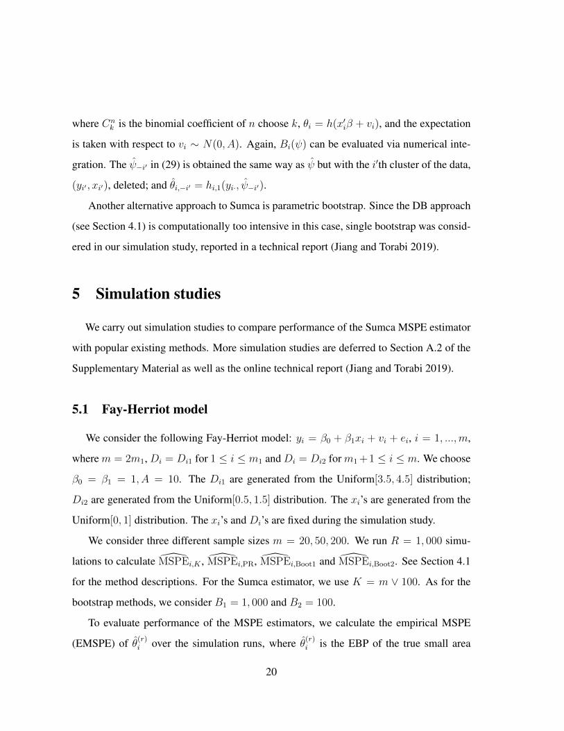
5 Simulation studies

We carry out simulation studies to compare performance of the Sumca MSPE estimator

with popular existing methods. More simulation studies are deferred to Section A.2 of the

Supplementary Material as well as the online technical report (Jiang and Torabi 2019).

5.1 Fay-Herriot model

We consider the following Fay-Herriot model: yi = β0 + β1xi + vi + ei, i = 1, ...,m,

where m = 2m1, Di = Di1 for 1 ≤ i ≤ m1 and Di = Di2 for m1 +1 ≤ i ≤ m. We choose

β0 = β1 = 1, A = 10. The Di1 are generated from the Uniform[3.5, 4.5] distribution;

Di2 are generated from the Uniform[0.5, 1.5] distribution. The xi’s are generated from the

Uniform[0, 1] distribution. The xi’s and Di’s are fixed during the simulation study.

We consider three different sample sizes m = 20, 50, 200. We run R = 1, 000 simu-

lations to calculate MSPEi,K , MSPEi,PR, MSPEi,Boot1 and MSPEi,Boot2. See Section 4.1

for the method descriptions. For the Sumca estimator, we use K = m ∨ 100. As for the

bootstrap methods, we consider B1 = 1, 000 and B2 = 100.

To evaluate performance of the MSPE estimators, we calculate the empirical MSPE

(EMSPE) of θ(r)i over the simulation runs, where θ(r)

i is the EBP of the true small area

20

mean, θ(r)i , for the rth simulation run, r = 1, . . . , R. Specifically, we have

EMSPE =1

R

R∑r=1

{θ(r)i − θ

(r)i }2, i = 1, ...,m; (31)

The percentage relative bias (% RB) of a MSPE estimator, MSPE, is defined as

% RB = 100× [{E(MSPE)− EMSPE}/EMSPE], (32)

where E(MSPE) is the average of the simulated MSPE.

Figure 1 shows that all four methods perform very well in terms of %RB for different

number of small areas. Comparatively, the bias of the Prasad-Rao estimator tend to be more

negative, indicating (slight) underestimation, while that of the Sumca estimator tend to be

more positive, indicating (slight) overestimation. See Figure A.2 of the Supplementary

Material for illustration. Especially for m = 50, the median %RB of PR and Sumca

methods seem to be closer to zero than the DB methods. Note that we only compare with

DB for m = 20 and 50, as DB gets computationally more intensive for larger m.

Following Slud and Maiti (2006), we also consider variability of the MSPE estimators

for different m. It was found that Sumca estimator is very stable for different m. See

Section A.2 of the Supplementary Material for detail.

It should be noted that the Prasad-Rao MSPE estimator is specifically derived to in-

corporate the Prasad-Rao estimator of A (Prasad and Rao 1990); on the other hand, our

unified Sumca approach applies to any procedure of parameter estimation, including the

special case of Prasad-Rao estimator. Furthermore, our simulation results show that, when

it comes to this special case, Sumca is as competitive as the method specifically designed

for the case. Again, see Section A.2 of the Supplementary Material for more detail.

Finally, although we have considered relatively small number of replications (K =

m ∨ 100) for the Sumca estimator (see the next section for discussion), the values of the

Sumca estimators were positive in all of the simulation runs, another desirable property for

an MSPE estimator (see Remark 1 in Section 2).

21

PR Boot1 Boot2 Sumca

−1

0−

50

51

01

5

PR Boot1 Boot2 Sumca

−5

05

10

●

●

●

●

●

●

●

●

PR Sumca−0.0

6−0

.02

0.00

0.02

0.04

0.06

(a) (b) (c)Figure 1: Boxplots of % RB of MSPE estimates using Sumca, DB (Boot1 and Boot2) and

PR methods: (a) m = 20; (b) m = 50; (c) m = 200.

5.2 Area-level model with model selection

We carry out a simulation study to compare performance of the Sumca estimator with

the DHM estimator in a PMS situation (see Section 3). As described earlier, DHM pro-

posed model selection by testing for the presence of the area-specific random effects or,

equivalently, H0 : A = 0 before determining which SAE method to use (see Section 4.2).

The data are generated under the following model: yi = β01+β1xi+vi+ei, 1 ≤ i ≤ m1;

yi = β02 + β1xi + vi + ei, m1 + 1 ≤ i ≤ m, where the vi’s and ei’s satisfy the assumptions

of the Fay-Herriot model, Di = Di1 for 1 ≤ i ≤ m1 and Di = Di2 for m1 + 1 ≤ i ≤ m

with m = 2m1. The parameters β01, β02 are to be determined later, β1 = 1, and three

different true values of A are considered: A = 0, 0.5, 1. The Di1 are generated from

the Uniform[0.5, 1.5] distribution and Di2 are from the Uniform[15.5, 16.5] distribution.

The xi’s are generated from the Uniform [0, 1] distribution. The Di’s and xi’s are fixed

throughout the simulation study.

The model we are fitting, however, is the standard Fay-Herriot model (19) with x′iβ =

β0 + β1xi, where the xi, Di are as above, and β0, β1, A are unknown fixed effects. In other

words, there is a potential model misspecification (in assuming that β01 = β02 = β0),

22

but we pretend that this is not known. Following a suggestion by Molina, Rao and Datta

(2015), we consider α = 0.2 as the level of significance in testing A = 0. Other than the

hypothesis testing, the SAE method is the same as in the previous subsection; in particular,

we consider the Prasad-Rao estimators of A and β, as described below (21).

We first consider a case where there is no model misspecification, that is, β01 = β02 =

β0 = 1. The main purpose is study performance of Sumca (and DHM) as the sample size,

m, increases, when the underlying model is correct. We consider m = 20, 50, 100. We

compare performance of Sumca and DHM methods in terms of %RB. We use K = 100 for

the Sumca estimator. The results, based on R = 1, 000 simulation runs, are illustrated by

Figure 2; some summary statistics are reported in Table 1. Both the figure and table show

the improved performance of Sumca as m increases, both in terms of the mean (median)

and especially in term of the standard deviation of the %RB. This is what the asymptotic

theory has predicted (see Theorem 4). Overall, the performance of DHM improves, too, as

m increases, although, comparatively, Sumca performs much better than DHM, especially

under the alternatives. The average %RB over the small areas appears to be positive for

DHM, and negative for Sumca. The empirical probability of rejection in the hypothesis test

is also reported in Table 1. The test appears to perform very well.

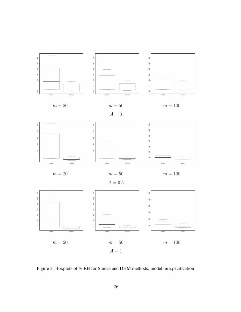
Next, we consider the case that the underlying model is misspecified, that is, β01 =

1, β02 = 4. It should be noted that the theory (both Theorem 3 and Theorem 4) is estab-

lished under the assumption that there is no model misspecification other than the part that

is subject to model selection. Thus, the asymptotic theory does not predict the behavior of

Sumca in this case. Nevertheless, we can still compare the relative performance of Sumca

and DHM in this case. Figure 3, which is also based on R = 1, 000 simulation runs, shows

that, in all scenarios, Sumca still performs better than DHM, especially under the alterna-

tive, although the difference is somewhat less striking compared to the case of no model

misspecification. It is also seen that the difference between the two methods is more signif-

23

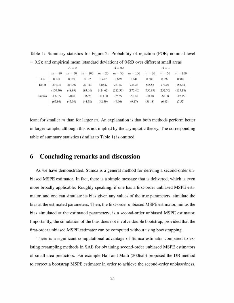
Table 1: Summary statistics for Figure 2: Probability of rejection (POR; nominal level

= 0.2); and empirical mean (standard deviation) of %RB over different small areasA = 0 A = 0.5 A = 1

m = 20 m = 50 m = 100 m = 20 m = 50 m = 100 m = 20 m = 50 m = 100

POR 0.178 0.197 0.192 0.457 0.629 0.841 0.688 0.897 0.988

DHM 201.04 211.86 271.43 440.42 267.57 234.23 545.58 274.01 153.34

(150.70) (48.99) (93.04) (424.62) (212.36) (175.40) (556.89) (252.70) (135.18)

Sumca -137.77 -90.61 -16.28 -111.08 -75.99 -50.46 -98.48 -66.08 -42.75

(67.86) (47.09) (44.58) (42.39) (9.96) (9.17) (31.18) (6.43) (7.52)

icant for smaller m than for larger m. An explanation is that both methods perform better

in larger sample, although this is not implied by the asymptotic theory. The corresponding

table of summary statistics (similar to Table 1) is omitted.

6 Concluding remarks and discussion

As we have demonstrated, Sumca is a general method for deriving a second-order un-

biased MSPE estimator. In fact, there is a simple message that is delivered, which is even

more broadly applicable: Roughly speaking, if one has a first-order unbiased MSPE esti-

mator, and one can simulate its bias given any values of the true parameters, simulate the

bias at the estimated parameters. Then, the first-order unbiased MSPE estimator, minus the

bias simulated at the estimated parameters, is a second-order unbiased MSPE estimator.

Importantly, the simulation of the bias does not involve double bootstrap, provided that the

first-order unbiased MSPE estimator can be computed without using bootstrapping.

There is a significant computational advantage of Sumca estimator compared to ex-

isting resampling methods in SAE for obtaining second-order unbiased MSPE estimators

of small area predictors. For example Hall and Maiti (2006ab) proposed the DB method

to correct a bootstrap MSPE estimator in order to achieve the second-order unbiasedness.

24

DHM Sumca

−2

00

02

00

40

06

00

DHM Sumca−

20

00

20

04

00

60

0DHM Sumca

−2

00

02

00

40

06

00

m = 20 m = 50 m = 100

A = 0

DHM Sumca

05

00

10

00

DHM Sumca

05

00

10

00

DHM Sumca

05

00

10

00

m = 20 m = 50 m = 100

A = 0.5

DHM Sumca

05

00

10

00

15

00

DHM Sumca

05

00

10

00

15

00

DHM Sumca

05

00

10

00

15

00

m = 20 m = 50 m = 100

A = 1

Figure 2: Boxplots of % RB for Sumca and DHM methods; no model misspecification

25

DHM Sumca

−100

010

020

030

040

050

0

DHM Sumca−1

000

100

200

300

400

500

DHM Sumca

−100

010

020

030

040

050

0

m = 20 m = 50 m = 100

A = 0

DHM Sumca

020

040

060

080

010

00

DHM Sumca

020

040

060

080

010

00

DHM Sumca

020

040

060

080

010

0012

00

m = 20 m = 50 m = 100

A = 0.5

DHM Sumca

020

040

060

080

010

0012

00

DHM Sumca

020

040

060

080

010

0012

00

DHM Sumca

020

040

060

080

010

00

m = 20 m = 50 m = 100

A = 1

Figure 3: Boxplots of % RB for Sumca and DHM methods; model misspecification

26

The procedure is computationally very intensive. Jiang et al. (2018) proposed the McJack

method, which requires the Monte-Carlo sample size, K, to satisfy m2/K → 0. However,

for the Sumca estimator it is only suggested that K = m (see the next paragraph). The

computational saving by Sumca is mainly due to the following simple fact: If a term is al-

ready O(m−1), a simple plug-in estimator will “do the trick”, that is, produce an estimator

of the term whose bias is o(m−1); in other words, no bias correction is needed for this term.

For Sumca, this term is d(ψ) = b(ψ) − c(ψ) defined above (4), and no bias correction is

needed after the plugging-in [see (4)]. The more intensive computational efforts of DB and

McJack are spent on bias-correcting terms of O(m−1), which is not necessary, so far as the

second-order unbiasedness is concerned. In Sumca, the “plugging-in principle” is executed

with the assistance of Monte-Carlo simulation.

As mentioned (second paragraph of Section 1), the current SAE literature has focused

on (approximate) unbiasedness in MSPE estimation; little has been done regarding variance

in the MSPE estimation. It was noted that the choice of K does not affect the second-order

unbiasedness of the Sumca estimator. The following discussion is regarding the variance

aspect. First, the Monte-Carlo part of the Sumca estimator, that is, the second term on the

right side of (13), is not the main contributor to the variance. To see this, note that, with

respect to the joint distribution of the data and Monte-Carlo sampling, we have

var(MSPEK) = var{

E(MSPEK |y)}

+ E{

var(MSPEK |y)}. (33)

Furthermore, by the way that the Monte-Carlo samples are drawn, we have

var(MSPEK |y) = K−1var{a(y[1], ψ)− a(y[1], ψ[1])|y}, (34)

hence, the second term on the right side of (33) is O(K−1). On the other hand, we have

E(MSPEK |y) = a(y, ψ) + E{a(y[1], ψ)− a(y[1], ψ[1])|y} = a(y, ψ) + d(ψ) (35)

27

by the definition of d(ψ) and the way the Monte-Carlo samples are drawn. The variance of

d(ψ) is typically O(m−1). Thus, by (33)–(35), we have, by the Cauchy-Schwarz inequality

var(MSPEK) = var{a(y, ψ)}+O(m−1/2)

√var{a(y, ψ)}+O(m−1 +K−1). (36)

According to our earlier result [see the paragraph between (7) and (11)], the order of

var{a(y, ψ)} is O(m−1) under the general linear mixed model (10), with θ being a linear

mixed effect, and θ the EBP of θ. In a PMS situation, suppose that θ is the EBP under

the selected model, M . If the model selection procedure is consistent, then with high

probability (e.g., Theorem 5 of Jiang and Torabi 2019), one has M = Mo, where Mo the

true underlying model. It follows that, with high probability, θ becomes the EBP; therefore,

the order O(m−1) is still expected for var{a(y, ψ)} in this situation.

In general, as long as var{a(y, ψ)} = O(m−1) holds, by (36), to ensure that the order

of the variance of the Sumca estimator does not increase due to K, the latter should be of

the same order as m. A simple choice would be K = m.

On the other hand, it should be noted that var{a(y, ψ)} = O(m−1) is not always ex-

pected to hold. For example, in the case of mixed logistic model, discussed in Section 4.3,

one has the expression a(y, ψ) = var(θi|y)|ψ=ψ, which depends on yi· =∑ni

j=1 yij , in addi-

tion to ψ. Thus, in this case, the variance of a(y, ψ) is expected to be O((m∧ ni)−1) rather

than O(m−1). However, by (36), one can see that K = m is still a good choice to ensure

that the variance contribution due to the Monte-Carlo part is, at most, the same order as

that due to the leading term, a(y, ψ).

We shall explore the variance issue more broadly, including the situation where the

variance of a(y, ψ) may not be O(m−1), with a rigorous treatment, in our future work.

Another issue regarding the MSPE estimation is how to obtain accurate MSPE estima-

tion under model misspecification. In the case of PMS (see Section 3), our approach is

based on existence of a full model, which is a correct model. However, the issue can also

28

arise in a non-model-selection context, where the underlying model is misspecified. See

Liu, Ma and Jiang (2019).

Acknowledgements. The research of Jiming Jiang is partially supported by the NSF

grant DMS-1510219. The research of Mahmoud Torabi is supported by a grant from the

Natural Sciences and Engineering Research Council of Canada (NSERC). The authors

are grateful to an Associate Editor and two referees for their constructive comments and

suggestions that have led to major improvement of the work as well as presentation.

References

[1] Das, K. and Jiang, J. and Rao, J. N. K. (2004), Mean squared error of empirical

predictor, Ann. Statist. 32, 818-840.

[2] Datta, G. S., Hall, P., and Mandal, A. (2011), Model selection by testing for the

presence of small-area effects, and applications to area-level data, J. Amer. Statist.

Assoc. 106, 361-374.

[3] Datta, G. S. and Lahiri, P. (2000), A unified measure of uncertainty of estimated best

linear unbiased predictors in small area estimation problems, Statistica Sinica 10,

613-627.

[4] Datta, G. S. and Rao, J. N. K. and Smith, D. D. (2005), On measuring the variability

of small area estimators under a basic area level model, Biometrika 92, 183-196.

[5] Fay, R. E. and Herriot, R. A. (1979), Estimates of income for small places: an appli-

cation of James-Stein procedures to census data, J. Amer. Statist. Assoc. 74, 269-277.

[6] Hall, P. and Maiti, T. (2006a), Nonparametric estimation of mean-squared prediction

error in nested-error regression models, Ann. Stat. 34, 1733-1750.

29

[7] Hall, P. and Maiti, T. (2006b), On parametric bootstrap methods for small area pre-

diction, J. Roy. Statist. Soc. Ser. B 68, 221-238.

[8] Jiang, J. (2001), Mixed effects models with random cluster sizes, Statist. Probab.

Letters 53, 201–206.

[9] Jiang, J. (2007), Linear and Generalized Linear Mixed Models and Their Applica-

tions, Springer, New York.

[10] Jiang, J. (2010), Large Sample Techniques for Statistics, Springer, New York.

[11] Jiang, J. (2017), Asymptotic Analysis of Mixed Effects Models: Theory, Applications,

and Open Problems, Chapman & Hall/CRC.

[12] Jiang, J. and Lahiri, P. (2001), Empirical best prediction for small area inference with

binary data, Ann. Inst. Statist. Math. 53, 217-243.

[13] Jiang, J., Lahiri, P. and Nguyen, T. (2018), A unified Monte-Carlo jackknife for small

area estimation after model selection, Ann. Math. Sci. Appl. 3, 405-438.

[14] Jiang, J., Lahiri, P. and Wan, S. (2002), A unified jackknife theory for empirical best

prediction with M-estimation, Ann. Statist. 30, 1782-1810.

[15] Jiang, J., Nguyen, T., and Rao, J. S. (2015), The E-MS algorithm: Model selection

with incomplete data, J. Amer. Statist. Assoc. 110, 1136-1147.

[16] Jiang, J., Rao, J. S., Gu, Z. and Nguyen, T. (2008), Fence methods for mixed model

selection, Ann. Statist. 36, 1669-1692.

[17] Jiang, J. and Torabi (2019), Sumca: Simple, unified, Monte-Carlo assisted approach

to second-order unbiased MSPE estimation, Technical Report.

30

[18] Liu, X., Ma, H. and Jiang, J. (2019), Assessing uncertainty involving model misspec-

ification: A one-bring-one route, Technical Report.

[19] Molina, I., Rao, J.N.K. and Datta, G.S. (2015), Small area estimation under a Fay-

Herriot model with preliminary testing for the presence of random effects, Surv.

Methodol. 41, 1-19.

[20] Muller, S., Scealy, J. L., and Welsh, A. H. (2013), Model selection in linear mixed

models, Statist. Sci. 28, 135-167.

[21] Pfeffermann, D. (2013), New important developments in small area estimation,

Statist. Sci. 28, 40-68.

[22] Prasad, N. G. N. and Rao, J. N. K. (1990), The estimation of mean squared errors of

small area estimators, J. Amer. Statist. Assoc. 85, 163-171.

[23] Rao, J. N. K. and Molina, I. (2015), Small Area Estimation, 2nd ed., Wiley, New York.

[24] Shao, J. and Tu, D. (1995), The Jackknife and Bootstrap, Springer, New York.

[25] Slud, E.V. and Maiti, T. (2006), Mean-squared error estimation in transformed Fay-

Herriot models, J. Roy. Statist. Soc. Ser. B 68, 239-257.

[26] Tibshirani, R. J. (1996), Regression shrinkage and selection via the Lasso, J. Roy.

Statist. Soc. Ser. B 58, 267-288.

31