Substation Location and Transmission Network Expansion … · 2017-07-26 · Substation Location...
26
Substation Location and Transmission Network Expansion Problem in Power System Meltem Peker a , Ayse Selin Kocaman a , Bahar Y. Kara a,* a Department of Industrial Engineering, Bilkent University, 06800 Ankara, Turkey [email protected], [email protected], [email protected] * * Corresponding author. Phone number: +90 312 290 3156 In this paper, we propose a model for the generation and transmission network expansion plan- ning problem that includes decisions related to substations’ locations and sizes. In power system expansion planning problems, locations of generation units and/or transmission lines are deter- mined. However, substation location decisions are not explicitly studied. Nevertheless, including the decisions of substations’ locations and sizes to the problem can change the transmission net- work substantially. Hence, in this study, we first discuss the benefit of incorporating substation decisions to the transmission network design problem. We then propose a model that finds a minimum cost network, the optimal locations and sizes of substations and generation plants. To overcome the computational challenge of the proposed model, we present a heuristic solution approach, in which we decompose the multi-period problem into several single-period problems that are solved sequentially. Computational studies on 24-bus and 118-bus power systems show that the proposed solution approach yields near optimal solutions in minutes. Keywords : location, network expansion, integrated planning, transmission switching. 1. Introduction The goal of the transmission network expansion planning (TNEP) problem is to determine optimal dispatch of the power and find the optimal design of a network by expanding an existing network. Considering continuously increasing demand, expanding or reinforcing existing gener- ation units (generation expansion planning-GEP) is also studied in the literature. For long-term planning, in practice, generation resources are planned first, and based on the solution, trans- mission network is planned [1]. In the literature, there are also studies which consider generation and transmission network expansion planning (GTNEP) problems simultaneously to find a less costly solution which may not be obtained in the sequential approach. In GTNEP problems, although generation and transmission decisions are assessed simulta- neously, substation components, which can be used to increase/decrease the voltage of the power at critical locations, are not explicitly included to the models. Investment cost of substations are either ignored or considered to be included in the investment costs of the generation units or transmission lines. However, including substations’ locations and sizes to the GTNEP problem can change the transmission network substantially, and an integrated multi-period power system 1
Transcript of Substation Location and Transmission Network Expansion … · 2017-07-26 · Substation Location...

Substation Location and Transmission Network Expansion
Problem in Power System
Meltem Pekera, Ayse Selin Kocamana, Bahar Y. Karaa,∗aDepartment of Industrial Engineering, Bilkent University, 06800 Ankara, [email protected], [email protected], [email protected]∗
∗ Corresponding author. Phone number: +90 312 290 3156
In this paper, we propose a model for the generation and transmission network expansion plan-
ning problem that includes decisions related to substations’ locations and sizes. In power system
expansion planning problems, locations of generation units and/or transmission lines are deter-
mined. However, substation location decisions are not explicitly studied. Nevertheless, including
the decisions of substations’ locations and sizes to the problem can change the transmission net-
work substantially. Hence, in this study, we first discuss the benefit of incorporating substation
decisions to the transmission network design problem. We then propose a model that finds a
minimum cost network, the optimal locations and sizes of substations and generation plants. To
overcome the computational challenge of the proposed model, we present a heuristic solution
approach, in which we decompose the multi-period problem into several single-period problems
that are solved sequentially. Computational studies on 24-bus and 118-bus power systems show
that the proposed solution approach yields near optimal solutions in minutes.
Keywords: location, network expansion, integrated planning, transmission switching.
1. Introduction
The goal of the transmission network expansion planning (TNEP) problem is to determine
optimal dispatch of the power and find the optimal design of a network by expanding an existing
network. Considering continuously increasing demand, expanding or reinforcing existing gener-
ation units (generation expansion planning-GEP) is also studied in the literature. For long-term
planning, in practice, generation resources are planned first, and based on the solution, trans-
mission network is planned [1]. In the literature, there are also studies which consider generation
and transmission network expansion planning (GTNEP) problems simultaneously to find a less
costly solution which may not be obtained in the sequential approach.
In GTNEP problems, although generation and transmission decisions are assessed simulta-
neously, substation components, which can be used to increase/decrease the voltage of the power
at critical locations, are not explicitly included to the models. Investment cost of substations
are either ignored or considered to be included in the investment costs of the generation units or
transmission lines. However, including substations’ locations and sizes to the GTNEP problem
can change the transmission network substantially, and an integrated multi-period power system
1

planning that also includes substations could result in a different network configuration. To the
best of our knowledge, there is no study that focuses on multi-period expansion of the GTNEP
problem that includes substations explicitly. With the aim of filling this gap in the literature,
in this work, we study an integrated generation, substation and transmission network expansion
planning problem (GSTNEP).
In most of the large electricity networks, transmission is designed as a static system and
the main aim is to determine power flows over a fixed network to minimize the total cost
[2]. On the other hand, switching transmission lines (taking some lines out of operation) is a
common practice in TNEP problems to increase transfer capacity, decrease power loss during the
transmission or improve voltage profile of the nodes [3]. Transmission switching is important
in TNEP problems because adding even a zero-cost transmission line may decrease the total
capacity of the system and hence, may result with higher generator costs in order to satisfy the
demand of each node due to Kirchoff’s laws. Since considering substations in the power systems
can change the network structure, taking out (or not using) some lines may also be beneficial in
GSTNEP problem. Thus, in this paper, we integrated transmission switching to the proposed
model of GSTNEP.
1.1. Effect of including substations to GTNEP
In the power investment/expansion planning problems, different types of substations are
considered depending on the level of decomposition of the problem, such as generation (step-
up), transmission and distribution (step-down) substations [4]. Needless to say, when a new
generation plant is built, it is also necessary to build a substation to connect the plant to the
system. However, in GTNEP problems, the cost of these substations are not explicitly identified
and it is considered within the investment cost of the generation plants. In the power systems,
transmission substations are also required for routing power from generators to demand nodes
[4]. Similar to step-up substations, investment cost of transmission substations could be added to
the investment cost of transmission lines. However, these approaches for calculating investment
cost of substations may not correctly estimate the total investment cost since generation amount
at each plant (which also determines capacity of substations) and the number of transmission
lines connected to each transmission substations are not known in advance.
Albert et al. [4] study North American power grid which includes generation plants, major
substations and transmission lines. In their model, 14099 nodes are identified as substations for
the North American power system. Substations that have a single high-voltage transmission line
are identified as distribution substation, and substations that are located at a source of power are
referred as step-up substations. The remaining ones are classified as transmission substations.
In the paper, 1633 of 14099 nodes are distinguished as power plants (step-up substations), 2179
nodes are referred as distribution substations and the remaining ones are labeled as transmission
2

substations. In such a large power system, adding investment cost of substations to investment
cost of generation units or to investment cost of transmission lines may result with different
network structure, which may also have higher total investment cost.
In the following example, we discuss the value of explicitly modeling substations by com-
paring solutions of GTNEP and GSTNEP. We show that even in a small network (6-bus power
system), including substation decisions affects the network structure and changes the substa-
tions’ locations. For this example, demand of buses, and properties related to transmission lines
are adapted from [5]. Load of buses is taken as 1/4 of the loads given in [5]. Bus 6 is also
considered as a demand node with 10 MW load. In [5], there is only one transmission line type
with 100 MW capacity. In this example, we include one more transmission line type with 50
MW capacity and investment cost of the line is considered to be 144000 $/km. Three candidate
generation capacities and five candidate substation capacities are considered and the investment
costs of these units for each capacity type are given in Section 4. The model used to solve these
problems will be explained in detail in Section 3.
Figure 1a and Figure 1b presents the networks resulting from GTNEP and GSTNEP prob-
lems, respectively. In the GTNEP output, one generation plant at node 2, and 5 transmission
lines are built with the total cost of $229.64M (Figure 1a). Thick lines have 100 MW capac-
ity whereas the other lines have 50 MW capacity. Although it is not explicitly modeled in
GTNEP problem, there should be 3 substations: one for step-up substation at node 2 and two
for transmission substations at nodes 3 and 5, which are required to change the line type or to
re-increase voltage of power in order to decrease power loss due to long distances between the
nodes. We calculate the required capacities and cost of these substations with respect to the
generation amount and power flows. When the costs of substation units are added to the cost
of the GTNEP, the total cost turns out to be $261.08M. However, in the GSTNEP output, with
the same parameter setting, we have a star network solution (Figure 1b), i.e. power is directly
sent to all the demand nodes from generation plant at node 2. In this case, we have only one
substation at node 2 and 5 transmission lines. The total cost of GSTNEP is equal to $247.82M.
Hence, for this example, by integrating the subproblems, we decrease the total cost of the power
system by $13.26M.
One can question the effect of the investment cost of substations to the network structure
and to the total cost. Hence, in order to analyze this effect, we come up with a parametric
analysis by multiplying investment cost of substations with a factor, α. Figure 1c and Figure 1d
present the networks of GSTNEP problem when investment cost of substations are multiplied
by α=0.05, 0.3, respectively. In Table 1, we also show the results of all instances with the cost
distribution in terms of investment costs of generation, substation, lines, and operation and
maintenance (O&M) cost for both GTNEP and GSTNEP problems for α =0.05, 0.3 and 1.0.
α =1.0 corresponds to the original investment cost of substations. Under the columns GTNEP,
3

the values given in bold show the calculated substation cost depending on α.
When the investment cost of substations is small, (i.e. α = 0.05), the output of GSTNEP
is the same as GTNEP (Figure 1a and 1c). That is, the output of the model where investment
cost of substations are ignored (GTNEP) is the same with the one where they are explicitly
considered (GSTNEP). When α = 0.3, there are only two substations at nodes 2 and 5, and
there exist 5 transmission lines with only one of them being 100 MW capacity (Figure 1d).
Thus, even when α = 0.3, beside the locations of substations, capacity of transmission lines also
changes. For this case, the calculated cost of GTNEP after adding substations is 0.86% higher
than the cost of GSTNEP. When α = 1.0, value of integrating substation to the problem is more
obvious; total cost of GTNEP is 5.35% higher than the total cost of GSTNEP.
Figure 1: (a) Result of GTNEP (b) Result of GSTNEP (c) Result of GSTNEP for α = 0.05 (d)
Result of GSTNEP for α = 0.3
A similar analysis is also made by multiplying investment cost of transmission lines by
three and Figure 2 presents the networks resulting from GTNEP and GSTNEP problem for the
original and adapted cost of transmission lines. GTNEP output remains the same when the
investment cost of transmission lines is increased (Figure 2a). However, even in a small network,
GSTNEP output changes significantly as the investment cost of the lines is increased. When cost
of transmission lines are at original values, there are one generation unit, one step-up substation
and 5 transmission lines with only one of them being 100 MW capacity (Figure 2b). But, as the
cost increases, GSTNEP output changes and two generation units and two step-up substations
4
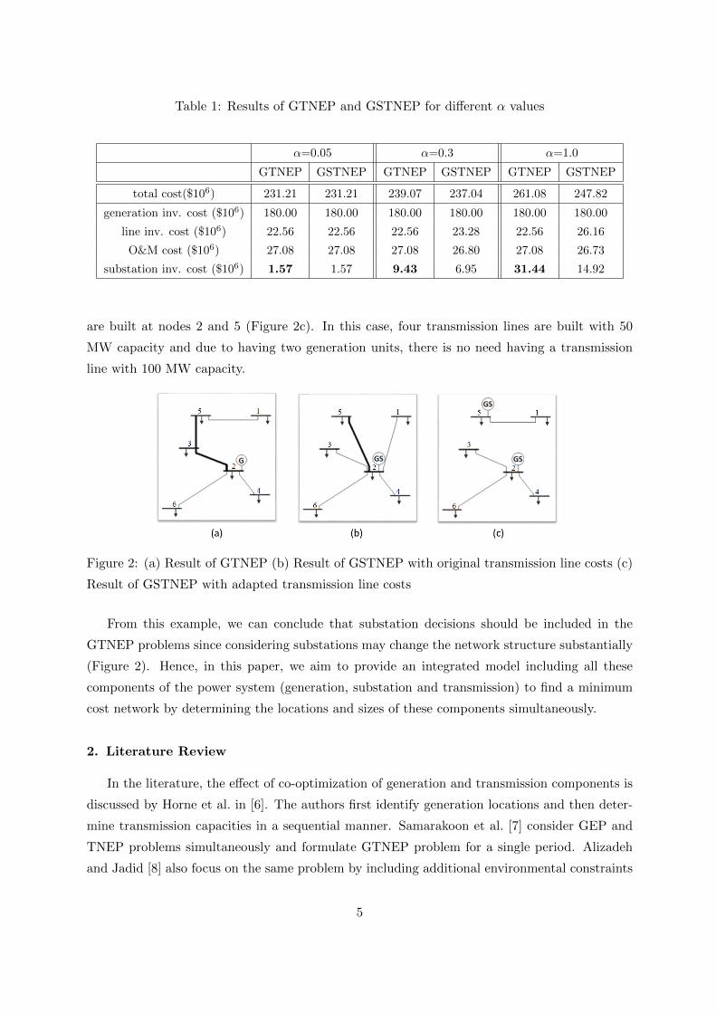
Table 1: Results of GTNEP and GSTNEP for different α values
α=0.05 α=0.3 α=1.0
GTNEP GSTNEP GTNEP GSTNEP GTNEP GSTNEP
total cost($106) 231.21 231.21 239.07 237.04 261.08 247.82
generation inv. cost ($106) 180.00 180.00 180.00 180.00 180.00 180.00
line inv. cost ($106) 22.56 22.56 22.56 23.28 22.56 26.16
O&M cost ($106) 27.08 27.08 27.08 26.80 27.08 26.73
substation inv. cost ($106) 1.57 1.57 9.43 6.95 31.44 14.92
are built at nodes 2 and 5 (Figure 2c). In this case, four transmission lines are built with 50
MW capacity and due to having two generation units, there is no need having a transmission
line with 100 MW capacity.
Figure 2: (a) Result of GTNEP (b) Result of GSTNEP with original transmission line costs (c)
Result of GSTNEP with adapted transmission line costs
From this example, we can conclude that substation decisions should be included in the
GTNEP problems since considering substations may change the network structure substantially
(Figure 2). Hence, in this paper, we aim to provide an integrated model including all these
components of the power system (generation, substation and transmission) to find a minimum
cost network by determining the locations and sizes of these components simultaneously.
2. Literature Review
In the literature, the effect of co-optimization of generation and transmission components is
discussed by Horne et al. in [6]. The authors first identify generation locations and then deter-
mine transmission capacities in a sequential manner. Samarakoon et al. [7] consider GEP and
TNEP problems simultaneously and formulate GTNEP problem for a single period. Alizadeh
and Jadid [8] also focus on the same problem by including additional environmental constraints
5
and fuel supply limitations. They analyze their method with 6-bus and 30-bus power systems.
In [9], the same authors consider a multi-period GTNEP problem including time as a new di-
mension to their previous model given in [8] and solve the new dynamic model using Benders
decomposition algorithm. Jenabi et al. [10] formulate a multi-period GTNEP problem consid-
ering demand side management technologies to reduce the peak demand. They also propose a
Benders decomposition algorithm to solve the problem. Guerra et al. [11] provide an integrated
model for GTNEP problem that includes renewable energy sources, demand side management
and CO2 emission constraints. The model is applied to Colombian interconnected power system
under different scenarios. Seddighi and Ahmadi-Javid [12] provide a stochastic programming
model for multi-period GTNEP problem and the uncertainties are related to demand, generation
amounts, cost and greenhouse gas emissions. They apply their model to 400-kV system of Iran’s
northwestern power grid which includes 17 nodes. Since long-term power investment/expansion
planning problems are complex, some researchers work on improving computational quality of
the problem. Munoz et al. [13] propose a new two-phase approach for GTNEP problem with
Benders decomposition. They develop new bounds for the expected system cost using Jensen’s
inequality. Mınguez and Garcıa-Bertrand [14] propose an algorithm for solving robust TNEP
problem. Grimm et al. [15] provide a model to analyze generation and transmission investment
decisions in electricity market. By defining single and multiple price zones, they compare their
solutions on 3-node and 6-node examples.
In the literature, there are a limited number of papers that study substation location and
transmission network expansion problems (STNEP) and in those studies, generation decisions
are included in the models. Cebeci et al. [16] work on a single period STNEP problem and de-
termine the locations of substations, their connections to demand points as well as the HV lines
between them. The authors also propose an algorithm that decomposes the problem into invest-
ment and feasibility-check subproblems. Akbari et al. [17] consider a scenario based stochastic
STNEP problem for a single period. Their problem includes finding the generation amounts at
prescribed generation plants, selection of new buses (can be considered as substations) and new
transmission lines. However, authors do not consider building new generation plants or include
some restrictions for the total incoming or outgoing power flow in the new buses. To solve the
problem, a scenario reduction technique is applied to decrease number of scenarios.
In addition to co-optimization of subproblems, by switching transmission lines (taking some
lines in and out of operation), total cost can be decreased. This transmission switching approach
(TS), is applied to many problems in different areas. Fisher et al. [2] are the first authors
that provide a mathematical programming model for TNEP problem considering TS. Hedman
et al. [3] present a formulation for generation unit commitment by considering transmission
switching. The authors decompose the problem into two subproblems by first solving their
model without switching for a 24-hour problem. Then, they determine the status of lines by
6
fixing unit commitment decisions. Khodaei et al. [18] provide a Benders decomposition algorithm
for solving GTNEP problem with transmission switching. By providing an existing network and
limiting number of switchable lines, they compare the solutions for different cases. Villumsen
and Philpott [19] add uncertainty to the TNEP problem with TS by a scenario approach. For
a static (single period) problem, the authors apply Dantzig-Wolfe decomposition algorithm to
the problem. Dehghan and Amjady [20] provide a new robust optimization model for TNEP
including energy storage systems and transmission switching.
As it is discussed in the previous section, including substation decisions may change the
topology of the network substantially. However, aforementioned studies show that in GTNEP
problems, decisions related to substation locations are not included. Similarly, in the STNEP
problems, power output from a substation is only dependent on the capacity of that substation
and generation expansion decisions are not included to the problem. It is obvious that modeling
substations in GTNEP problems may reduce the total cost. To the best of our knowledge, there
is no study that includes substation decisions in GTNEP problem and in this paper, we present
an integrated planning for generation, substation and transmission expansion planning problems
(GSTNEP) considering transmission switching (TS).
GSTNEP problem that we present is a multi-period power system planning problem. In this
paper, we propose a mixed integer linear programming model (MILP) with the aim of finding
the optimal siting, sizing and timing of power system’s generation, transmission and substation
components simultaneously. We also determine power flow paths and generation amounts for
each time period. In the literature, to overcome the computational challenge of the power
expansion planning, problem is decomposed into subproblems and the solution is obtained by
iteratively solving these subproblems [1]. In this study, we present a heuristic solution approach,
in which we decompose our integrated multi-period problem into a set of single period problems
as many as the number of expansion periods. Computational studies on 24-bus and 118-bus
power systems show that the proposed solution approach yields better results than the results
of traditional method which is based on decomposing the problem and solving the subproblems
sequentially.
The rest of the paper is organized as follows: In the next section, we provide the mathematical
model and solution approaches for the problem. We show and discuss the results of the proposed
model in Section 4. We also compare the results of our proposed solution approach with the
solutions that are obtained by sequentially solving the subproblems. The paper concludes with
Section 5.
7
3. GSTNEP Problem
Given the demand of nodes and possible generation amounts from different source types, we
aim to find optimal siting, sizing and timing of system components (generation plants, substation
units and lines) in order to fulfill power demand in a multi-period planning horizon. The problem
includes optimization of power generation amounts, power flows and flow directions on the
transmission lines considering transmission switching option. In the electrical power systems,
when a new generation plant is built, it is also necessary to build a substation to connect the
plant to the system in order to adjust or transform the voltage to the required level. So, if a
generation unit is located at a node, we need to guarantee that there is also a step-up substation
at the same node. Moreover, a node which connects other demand nodes or substations to
a generation unit (or to a step-up substation) also has a transmission substation in order to
transform/re-increase the voltage level.
Direct current (DC) approximation of Kirchhoff’s first and second laws, and a single load
scenario for one time period are considered in this study as in [7]-[11]. However, similar to
[18, 21], to have a better representation of the reality, we divide each time period into a set
of demand blocks to consider seasonality and variability of demand within year. In the model,
as customarily done in the literature [11], we also assume that a predetermined ratio of the
transferred power is lost due to line resistance and the ratio depends on line types. For brevity,
throughout the paper, we refer a node that has just substations as substation node, a node that
has substation and generation units as generation node and the remaining nodes (which have
no generation and substation units) as demand node.
3.1. Mathematical programming model of GSTNEP
We use the following notation for the mathematical programming model. Let G = (N,E) be
a graph where N is the node set for demand nodes and candidate nodes for locating generation
and substation units; and E is the candidate corridors for building transmission lines. The sets
and corresponding indices, parameters and decision variables used in the mathematical model
are shown in Table 2.
8
Table 2: Nomenclature
Sets Explanation and corresponding indices
N set of all nodes (i and j)
E set of corridors (e = i, j)Ω+(e) sending-end bus of corridor e
Ω−(e) receiving-end bus of corridor e
A set of line types (a)
C set of generation technologies (c)
S set of substations (s)
B set of load blocks (b)
T set of periods (t)
Param. Explanation of parameters
dibt demand of node i at load block b at period t (MW)
CapGict generation capacity in node i from source type c at period t (MW)
CapLa capacity of transmission line type a (MW)
CapSs capacity of substation type s (MVA)
c-invc investment cost of source type c ($)
c-omc operation&maintenance cost of source type c ($/MWh)
c-subs investment cost of substation type s ($)
c-linea investment cost of transmission line type a ($/km)
le distance of corridor e (km)
bea susceptance of line type a of corridor e (p.u.)
r discount rate
durbt duration of load block b at period t (h)
efa transmission loss on the line type a per unit flow
TI number of years in each period
Dec.Var. Explanation of decision variables
Xict 1 if source type c is located at node i at period t, 0 o.w.
Yicbt generation amount in node i from source type c at load block b at period t
Kist 1 if substation type s is located at node i at period t, 0 o.w.
Kit 1 if at least one substation is located at node i until period t, 0 o.w.
θibt voltage angle of node i at load block b at period t (rad)
Leat 1 if line type a is built at corridor e at period t, 0 o.w.
L′eabt 1 if line type a at corridor e is used at load block b at period t, 0 o.w.
feabt flow on line type a at corridor e at load block b at period t
9

The proposed model for GSTNEP (GSTNEP-M ) is as follows:
min zinv + zsub + zline + zom (1)
zinv =∑
t∈T (1 + r)−TI(t−1)∑
i∈N∑
c∈C c-invcXict
zsub =∑
t∈T (1 + r)−TI(t−1)∑
i∈N∑
s∈S c-subsKist
zline =∑t∈T
(1 + r)−TI(t−1)∑e∈E
∑a∈A
c-lineale(Leat − Leat-1)
zom =∑t∈T
(1 + r)−TI(t−1)κ(r,TI)∑i∈N
∑c∈C
∑b∈B
c-omcdurbtYicbt
s.t∑c∈C
Yicbt +∑
e∈E|Ω−(e)=i
∑a∈A
feabt−
∑e∈E|Ω+(e)=i
∑a∈A
(1 + efa)feabt = dibt ∀i ∈ N, b ∈ B, t ∈ T (2)
Yicbt ≤∑
t′∈T :t′≤t
CapGict′Xict′ ∀i ∈ N, c ∈ C, b ∈ B, t ∈ T (3)
∑e∈E|Ω+(e)=i
∑a∈A
(1 + efa)|feabt| ≤∑s∈S
∑t′∈T :t′≤t
CapSsKist′ ∀i ∈ N, b ∈ B, t ∈ T (4)
∑e∈E|Ω−(e)=i
∑a∈A|feabt| ≤
∑s∈S
∑t′∈T :t′≤t
CapSsKist′+
dibt(1−Kit) ∀i ∈ N, b ∈ B, t ∈ T (5)
− CapLaL′eabt ≤ (1 + efa)feabt ≤ CapLaL
′eabt ∀e ∈ E, a ∈ A, b ∈ B, t ∈ T (6)
feabt = beaL′eabt(θibt − θjbt) ∀e ∈ E, a ∈ A, b ∈ B, t ∈ T (7)
L′eabt ≤ Leat ∀e ∈ E, a ∈ A, b ∈ B, t ∈ T (8)
Xict ≤ Kit ∀i ∈ N, c ∈ C, t ∈ T (9)
Kit ≤∑s∈S
∑t′∈T :t′≤t
Kist′ ∀i ∈ N, t ∈ T (10)
Kist ≤ Kit ∀i ∈ N, s ∈ S, t ∈ T (11)
Kit-1 ≤ Kit ∀i ∈ N, t ∈ T (12)
Leat-1 ≤ Leat ∀e ∈ E, a ∈ A, b ∈ B, t ∈ T (13)
− π ≤ θibt ≤ π ∀i ∈ N, b ∈ B, t ∈ T (14)
θ1bt = 0 ∀b ∈ B, t ∈ T (15)
Lea0 = 0 ∀e ∈ E, a ∈ A, b ∈ B (16)
Ki0 = 0 ∀i ∈ N (17)
Xict ∈ 0, 1 , Yicbt ≥ 0, θibt unrestricted ∀i ∈ N, c ∈ C, b ∈ B, t ∈ T (18)
Kist ∈ 0, 1 ∀i ∈ N, s ∈ S, t ∈ T (19)
Kit ∈ 0, 1 , ∀i ∈ N, t ∈ T (20)
Leat, L′eabt ∈ 0, 1 , feabt unrestricted ∀e ∈ E, a ∈ A, b ∈ B, t ∈ T (21)
The objective function (1) minimizes net present value of total cost; the first three terms are
10

for the investment costs of generation plants, substation units and transmission lines, respec-
tively. The last term is for the O&M cost. The function κ(r,TI)=(1 + r)(1− (1 + r)−TI)/r is to
calculate the present value of annual cost that has TI years in each time period with interest rate
r [22]. We remark here that, the cost of losses is not explicitly modeled in the objective function
since it is inherently included within the O&M cost. Constraint (2) provides the power balance,
that is equivalent to Kirchhoff’s first law and implies conservation of the power at each node
(after adding losses on the transmission lines for the transferred power) for each time period.
Constraint (3) states that generation amount in node i, at load block b, at period t cannot exceed
the possible generation amount that could be produced from all of the generation units located
at node i until time period t. Constraints (4) and (5) limit the total flow leaving from and en-
tering to the substation node or generation node i with the capacity of the substations located
at that node. Constraint (6) is the capacity constraint for the transmission lines. Constraint (7)
represents the power flow constraints based upon the Kirchhoff’s second law and it determines
that the power flow on each line (if used) is equal to the susceptance of the line multiplied by
the difference of the phase angles of the nodes. Constraint (8) enforces that a line can be used
at period t, only if the line is built. Constraints (9) and (10) satisfy that if a generation plant is
built at node i, at least one step-up substation should also be built at the same node. Constraint
(11) guarantees that Kit should be 1 if there is at least one substation unit at node i at period
t. Constraints (12) and (13) couple time units. Constraint (14) sets limits on the voltage angles
at every node. Constraint (15) is the reference point for voltage profile of nodes, and without
loss of generality, node 1 is selected as the reference point. Constraints (16) and (17) are the
initial points that should be given due to constraints (12) and (13). Constraints (18)-(21) are
the domain constraints.
We remark here that, constraints (4), (5) and (7) are nonlinear. Similar to the linearization
techniques used in [23], we provide a linear formulation for the problem. In the linear model,
the flow amount on each line is expressed as the difference of two nonnegative flow variables
f+eabt and f−eabt:
feabt = f+eabt − f
−eabt ∀e ∈ E, a ∈ A, b ∈ B, t ∈ T (22)
and the difference of voltage angles are expressed as the difference of two nonnegative variables
∆θ+ebt and ∆θ−ebt as follows:
θibt − θjbt = ∆θ+ebt −∆θ−ebt ∀e = i, j ∈ E, b ∈ B, t ∈ T (23)
By using the above substitutions, constraint (7) is linearized and replaced with the following
11

ones:
f+eabt ≤ bed∆θ+
ebt ∀e ∈ E, a ∈ A, b ∈ B, t ∈ T (24)
f−eabt ≤ bed∆θ−ebt ∀e ∈ E, a ∈ A, b ∈ B, t ∈ T (25)
f+eabt ≥ bed∆θ+
ebt −M(1− L′eabt) ∀e ∈ E, a ∈ A, b ∈ B, t ∈ T (26)
f−eabt ≥ bed∆θ−ebt −M(1− L′eabt) ∀e ∈ E, a ∈ A, b ∈ B, t ∈ T (27)
where M in (26) and (27) represents a sufficiently large number so that the new constraints
does not cut any feasible solution if the line e is not in operation.
In order to linearize |fedbt|, we utilize equation (22) and a linear expression of the absolute
value in constraints (4) and (5) can be derived as follows:
|feabt| = f+eabt + f−eabt ∀e ∈ E, a ∈ A, b ∈ B, t ∈ T (28)
Thus, a mixed integer linear model for GSTNEP (GSTNEP-L) is as follows:
min zinv + zsub + zline + zom (1)
s.t (3), (8)-(20), (23)-(27)∑c∈C
Yicbt +∑
e∈E|Ω−(e)=i
∑a∈A
(f+eabt − f
−eabt)−∑
e∈E|Ω+(e)=i
∑a∈A
(1 + efa)(f+eabt − f
−eabt) = dibt ∀i ∈ N, b ∈ B, t ∈ T (2′)
∑e∈E|Ω+(e)=i
∑a∈A
(1 + efa)(f+eabt + f−eabt) ≤∑
s∈S
∑t′∈T :t′≤t
CapSsKist′ ∀i ∈ N, b ∈ B, t ∈ T (4′)
∑e∈E|Ω−(e)=i
∑a∈A
(f+eabt + f−eabt) ≤
∑s∈S
∑t′∈T :t′≤t
CapSsKist′+
dibt(1−Kit) ∀i ∈ N, b ∈ B, t ∈ T (5′)
(1 + efa)f+eabt ≤ CapLaL
′eabt ∀e ∈ E, a ∈ A, b ∈ B, t ∈ T (6′)
(1 + efa)f−eabt ≤ CapLaL′eabt ∀e ∈ E, a ∈ A, b ∈ B, t ∈ T (6′′)
Leabt, L′eabt ∈ 0, 1 , f+
eabt ≥ 0, f−eabt ≥ 0 ∀e ∈ E, a ∈ A, b ∈ B, t ∈ T (21′)
∆θ+ebt ≥ 0,∆θ−ebt ≥ 0 ∀e ∈ E, b ∈ B, t ∈ T (29)
3.2. Strengthening the formulation
We also derive valid inequalities to strengthen the model.
Proposition 1. Inequality∑i∈N
dibt ≤∑i∈N
∑c∈C
∑t′∈T :t′≤t
CapGict′Xict′ ∀b ∈ B, t ∈ T (30)
is valid for GSTNEP-L.
12
The left hand side of the constraint (30) is the total demand in the power system for each
load block, at each period and the right hand side of the constraint is the total generation that
can be produced from all generation plants. Constraint (30) guarantees that total production
amount should meet the total demand in the system for each load block.
Proposition 2. The following inequality is valid for GSTNEP-L:∑c∈C
∑t′∈T :t′≤t
Xict′ +∑
e∈E|Ω−(e)=i
∑a∈A
L′eabt ≥ 1 ∀i ∈ N, b ∈ B, t ∈ T (31)
If there is no generation plants at node i at period t (Xict′ = 0 ∀ c ∈ C and t′ ≤ t), from
constraint (2’) there should be power entering to node i. Thus, due to constraints (6′) and (6′′),
there should also be at least one transmission line in operation entering to node i to transmit
the power entering to the same node.
3.3. Solution approaches
As explained in Section 1, power system expansion planning problems are highly complex
and nonlinear problems. Thus, to overcome the computational burden of the problems, dividing
the original problem into subproblems and solving these subproblems sequentially based on the
output of previous subproblem is a widely used approach in the literature. In this study, we
also propose a heuristic approach for the integrated GSTNEP problem to be able to solve larger
instances within reasonable solution times. In the computational study, the solutions of the
proposed model and heuristic are compared with the solutions obtained using the traditional
method in which the subproblems are solved sequentially. We remark here that, solving the
model in a sequential manner is also actually solving the GSTNEP problem heuristically since
this approach also requires decomposing and optimizing the subproblems of GSTNEP. The
sequential solution approach and the proposed time-based solution approach are explained below.
3.3.1. Sequential approach
In this approach, first, the GTNEP problem is solved and decisions related to power flows,
transmission lines, generation units and generation amounts are determined. Then, based on the
output of GTNEP, we determine the location and capacities of substation units, and calculate
the cost of these substations. In order to obtain GTNEP problem, we remove the constraints
that are related to substations from GSTNEP-L; that is, constraints (4′) and (5′) which are
related to capacity limitation of substations, constraints (9)-(12) which are the relationship
constraints between generation units and substations, and domain constraints ((17), (19) and
(20)). The remaining constraints of the GSTNEP-L constitutes a model for the GTNEP problem
and referred as GTNEP-L:
13
min zinv + zline + zom (32)
s.t (2′), (3), (6′), (6′′)(8), (13)-(16), (18), (21′), (23)-(27), (29)
X, G, f+, f−, L and L′ are the outputs of GTNEP-L and optimum solution value is denoted by
zGTNEP. Then, based on the values of these decision variables, K and K are determined. Total
investment cost of substations (zsub) is also calculated and denoted by zSUB. Hence, at the end
of this procedure, we obtain a solution for the original problem (GSTNEP) using the sequential
solution approach. The corresponding objective value for the solution is equal to zGTNEP+zSUB.
3.3.2. Time-based approach
We develop a time-based heuristic solution approach for the GSTNEP problem. In the
proposed heuristic, instead of dividing the problem into subproblems with respect to system
components, we decompose our multi-period problem into a set of single period problems as
many as the number of expansion periods (|T |) considered.
In this approach, we first define a problem for each time period t and refer it Single Period
Expansion Problem (SPEPt). In SPEPt, we consider only the first t periods and ignore the
remaining ones. For period t, we know all the investment decisions (generation units, substations
and lines), generation amounts and power flows up to period t, which are obtained from the
solution of SPEPt-1, and these variables are fixed in SPEPt. Then, we obtain the investment
decisions, generation amounts and power flows at period t by solving SPEPt. All the one-period
expansion problems (SPEP1, SPEP2, ... SPEP|T|) are solved iteratively by feeding the result of
a period as an existing infrastructure for the next time period in a nested manner. Hence, after
solving SPEP|T|, we obtain a solution for the original GSTNEP problem. For time period t, (or
when |T|=t), the model of SPEPt is given below.
min zinv + zsub + zline + zom (1)
s.t (2′), (3), (4′), (5′), (6′), (6′′), (8)-(20), (21′), (23)-(27), (29)
Xic1...Xict-1, Gicb1...Gicbt-1 are fixed ∀i ∈ N, b ∈ B, c ∈ C
Kis1...Kist-1 are fixed ∀i ∈ N, s ∈ S
Lea1...Leat-1 are fixed ∀e ∈ E, a ∈ A
f+eab1...f
+eat-1, f
−eab1...f
−eat-1 are fixed ∀e ∈ E, a ∈ A, b ∈ B
4. Computational Study
In this section, we introduce the data sets and parameters that are used in the computational
study. We test the combination of valid inequalities for the proposed model (GSTNEP-L) and
present the solution of the GSTNEP-L for 24-bus power system. In order to discuss the value
14
of integrating subproblems, we compare the results of GSTNEP-L along with the results of
the sequential and time-based solution approaches. We, then, discuss the effect of transmission
switching on the results. Lastly, we solve a large instance and present results of the sequential
and time-based solution approaches for 118-bus power system. For all the instances, we stopped
computations once the reported gap by the solver is less than 1%. All computation results are
obtained on a Linux environment with 2.4GHz Intel Xeon E5-2630 v3 CPU server with 64GB
RAM. All the experiments of the model and heuristics are implemented using Java Platform,
Standard Edition 8 Update 91 (Java SE 8u91) and Gurobi 6.5.1 in parallel mode using up to 32
threads.
4.1. 24-bus power system
The proposed model has been applied to a modified version of IEEE Reliability test system.
IEEE Reliability test system includes 24 nodes, 32 generation plants and 35 corridors for building
transmission lines [24]. A 15-year planning horizon is considered and divided into three time
periods of equal length. Demand of nodes at the initial time period (t=0) are the same as the
original demand values given in [24] for 24 bus. Annual demand growth rate is assumed to be
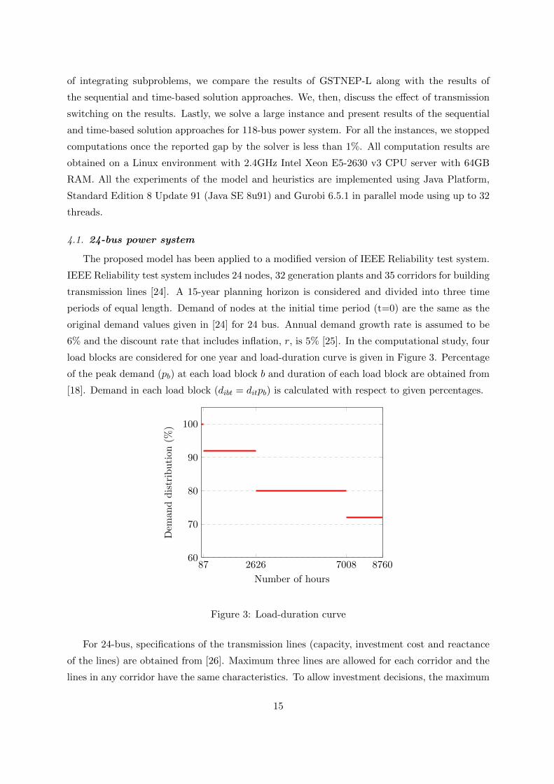
6% and the discount rate that includes inflation, r, is 5% [25]. In the computational study, four
load blocks are considered for one year and load-duration curve is given in Figure 3. Percentage
of the peak demand (pb) at each load block b and duration of each load block are obtained from
[18]. Demand in each load block (dibt = ditpb) is calculated with respect to given percentages.
87 2626 7008 876060
70
80
90
100
Number of hours
Dem
and
dis
trib
uti
on(%
)
Figure 3: Load-duration curve
For 24-bus, specifications of the transmission lines (capacity, investment cost and reactance
of the lines) are obtained from [26]. Maximum three lines are allowed for each corridor and the
lines in any corridor have the same characteristics. To allow investment decisions, the maximum
15
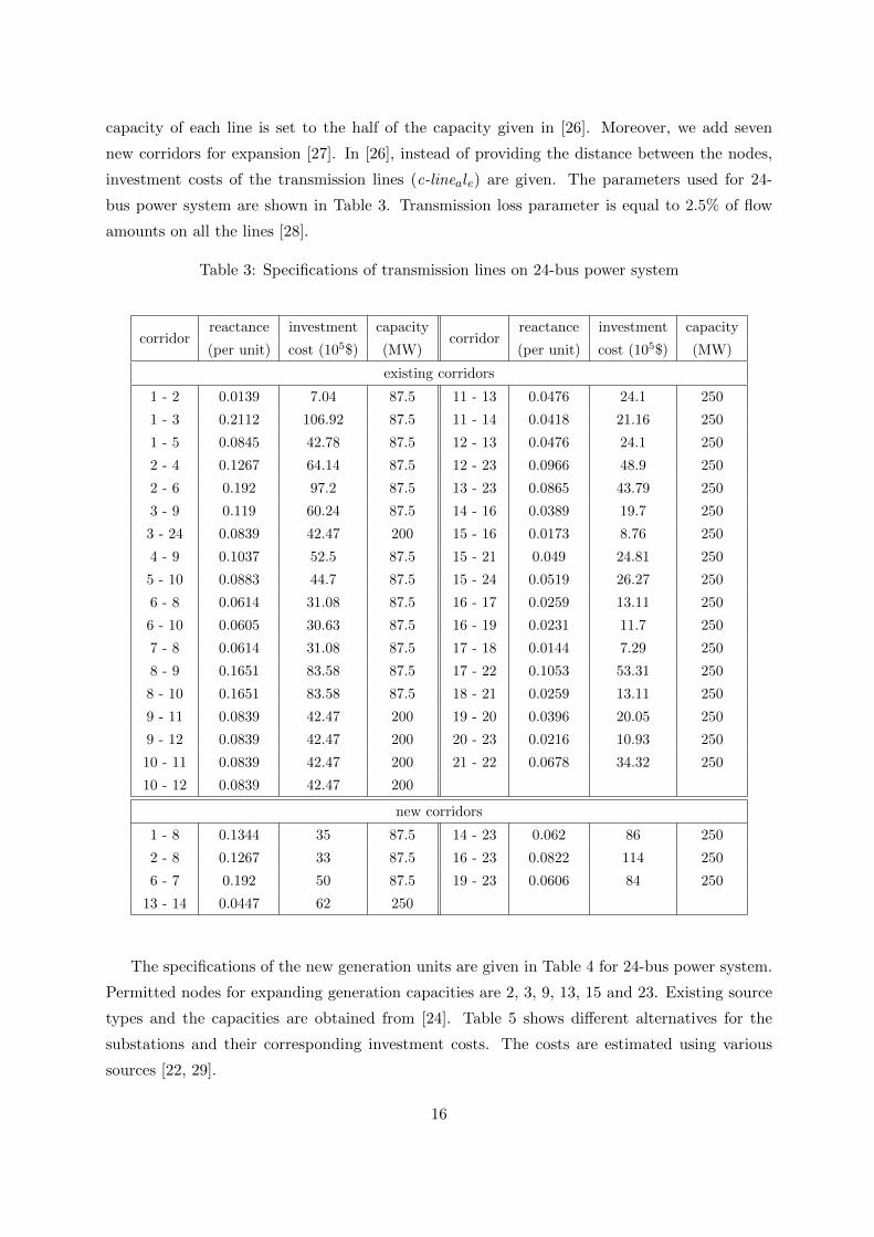
capacity of each line is set to the half of the capacity given in [26]. Moreover, we add seven
new corridors for expansion [27]. In [26], instead of providing the distance between the nodes,
investment costs of the transmission lines (c-lineale) are given. The parameters used for 24-
bus power system are shown in Table 3. Transmission loss parameter is equal to 2.5% of flow
amounts on all the lines [28].
Table 3: Specifications of transmission lines on 24-bus power system
corridorreactance investment capacity
corridorreactance investment capacity
(per unit) cost (105$) (MW) (per unit) cost (105$) (MW)
existing corridors
1 - 2 0.0139 7.04 87.5 11 - 13 0.0476 24.1 250
1 - 3 0.2112 106.92 87.5 11 - 14 0.0418 21.16 250
1 - 5 0.0845 42.78 87.5 12 - 13 0.0476 24.1 250
2 - 4 0.1267 64.14 87.5 12 - 23 0.0966 48.9 250
2 - 6 0.192 97.2 87.5 13 - 23 0.0865 43.79 250
3 - 9 0.119 60.24 87.5 14 - 16 0.0389 19.7 250
3 - 24 0.0839 42.47 200 15 - 16 0.0173 8.76 250
4 - 9 0.1037 52.5 87.5 15 - 21 0.049 24.81 250
5 - 10 0.0883 44.7 87.5 15 - 24 0.0519 26.27 250
6 - 8 0.0614 31.08 87.5 16 - 17 0.0259 13.11 250
6 - 10 0.0605 30.63 87.5 16 - 19 0.0231 11.7 250
7 - 8 0.0614 31.08 87.5 17 - 18 0.0144 7.29 250
8 - 9 0.1651 83.58 87.5 17 - 22 0.1053 53.31 250
8 - 10 0.1651 83.58 87.5 18 - 21 0.0259 13.11 250
9 - 11 0.0839 42.47 200 19 - 20 0.0396 20.05 250
9 - 12 0.0839 42.47 200 20 - 23 0.0216 10.93 250
10 - 11 0.0839 42.47 200 21 - 22 0.0678 34.32 250
10 - 12 0.0839 42.47 200
new corridors
1 - 8 0.1344 35 87.5 14 - 23 0.062 86 250
2 - 8 0.1267 33 87.5 16 - 23 0.0822 114 250
6 - 7 0.192 50 87.5 19 - 23 0.0606 84 250
13 - 14 0.0447 62 250
The specifications of the new generation units are given in Table 4 for 24-bus power system.
Permitted nodes for expanding generation capacities are 2, 3, 9, 13, 15 and 23. Existing source
types and the capacities are obtained from [24]. Table 5 shows different alternatives for the
substations and their corresponding investment costs. The costs are estimated using various
sources [22, 29].
16
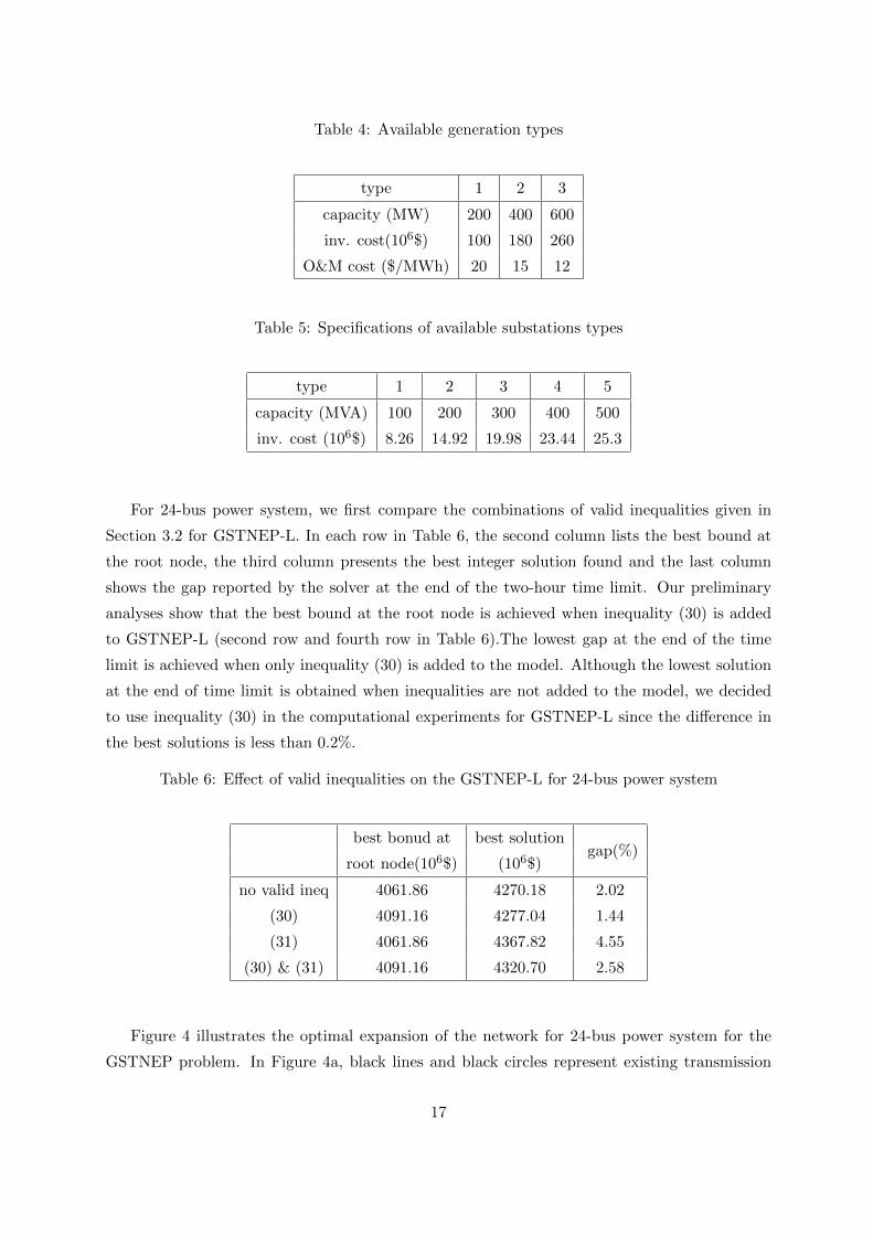
Table 4: Available generation types
type 1 2 3
capacity (MW) 200 400 600
inv. cost(106$) 100 180 260
O&M cost ($/MWh) 20 15 12
Table 5: Specifications of available substations types
type 1 2 3 4 5
capacity (MVA) 100 200 300 400 500
inv. cost (106$) 8.26 14.92 19.98 23.44 25.3
For 24-bus power system, we first compare the combinations of valid inequalities given in
Section 3.2 for GSTNEP-L. In each row in Table 6, the second column lists the best bound at
the root node, the third column presents the best integer solution found and the last column
shows the gap reported by the solver at the end of the two-hour time limit. Our preliminary
analyses show that the best bound at the root node is achieved when inequality (30) is added
to GSTNEP-L (second row and fourth row in Table 6).The lowest gap at the end of the time
limit is achieved when only inequality (30) is added to the model. Although the lowest solution
at the end of time limit is obtained when inequalities are not added to the model, we decided
to use inequality (30) in the computational experiments for GSTNEP-L since the difference in
the best solutions is less than 0.2%.
Table 6: Effect of valid inequalities on the GSTNEP-L for 24-bus power system
best bonud at best solutiongap(%)
root node(106$) (106$)
no valid ineq 4061.86 4270.18 2.02
(30) 4091.16 4277.04 1.44
(31) 4061.86 4367.82 4.55
(30) & (31) 4091.16 4320.70 2.58
Figure 4 illustrates the optimal expansion of the network for 24-bus power system for the
GSTNEP problem. In Figure 4a, black lines and black circles represent existing transmission
17
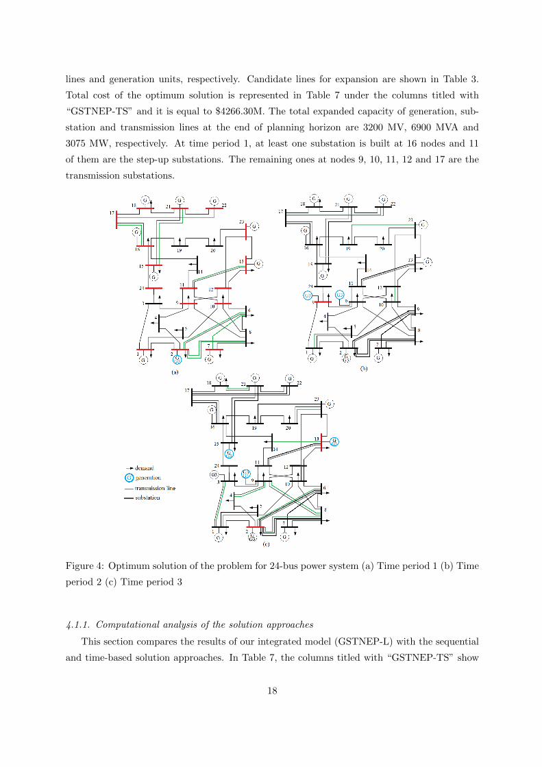
lines and generation units, respectively. Candidate lines for expansion are shown in Table 3.
Total cost of the optimum solution is represented in Table 7 under the columns titled with
“GSTNEP-TS” and it is equal to $4266.30M. The total expanded capacity of generation, sub-
station and transmission lines at the end of planning horizon are 3200 MV, 6900 MVA and
3075 MW, respectively. At time period 1, at least one substation is built at 16 nodes and 11
of them are the step-up substations. The remaining ones at nodes 9, 10, 11, 12 and 17 are the
transmission substations.
Figure 4: Optimum solution of the problem for 24-bus power system (a) Time period 1 (b) Time
period 2 (c) Time period 3
4.1.1. Computational analysis of the solution approaches
This section compares the results of our integrated model (GSTNEP-L) with the sequential
and time-based solution approaches. In Table 7, the columns titled with “GSTNEP-TS” show
18

the results of these three approaches for GSTNEP problem. As well as providing total cost, the
cost distribution in terms of investment costs of generation, substation and lines, and operation
and maintenance (O&M) cost are reported. We again note that, both approaches solve GSTNEP
problem heuristically.
We first compare the objective function values of solutions obtained with sequential and
time-based approaches. The proposed time-based approach finds a very good solution since the
gap from optimum solution is less than 1%. The solution of the sequential approach is larger
than the solution obtained with time-based approach and the difference between the result of
sequential approach and optimum solution is 3.86%. The optimum solution of GSTNEP problem
is found in approximately 12 hours. Time-based and sequential approaches find the solutions
in 2.3 minutes and 1.8 hours, respectively. Thus, in a very short time, the proposed time-based
approach finds a better solution than the solution obtained with sequential approach.
4.1.2. Analysis of transmission switching
In this section, we discuss the additional benefit of allowing transmission switching (TS).
We again compare the solutions of the three approaches; namely, the optimization model, the
sequential approach and the time-based approach.
In the original problem, GSTNEP, all the lines are considered as switchable. In order to
guarantee that line switching is not allowed, we added the following constraint to the model:
Leat ≤ L′eabt ∀e ∈ E, a ∈ A, b ∈ B, t ∈ T (33)
Constraint (33) guarantees that, if a line is built at t, then the line should be used in the same
period. With constraint (13), this requirement holds for all time periods.
In Table 7, we present the results for no TS case under the columns “GSTNEP-noTS”. In
sequential approach, in order not to allow switching lines, constraint (33) is also added to the
GTNEP-L. When TS is not allowed, we obtain similar results for the three solution methods;
GSTNEP-L has the lowest objective function value and the sequential solution approach has
the largest objective value. The difference between the results of GSTNEP-L and sequential
approach is 2.30%, whereas the difference between the solutions of GSTNEP-L and time-based
approach is 1.22%. For this case, we report the best solution that is obtained within 12 hours for
the GSTNEP-L and the gap reported by the solver is 1.48% at the end of 12 hours. Interestingly,
when TS is not allowed, the solution time of the sequential approach (20 seconds) is shorter than
the solution time of the proposed approach (13 minutes). We remark here that, in both cases
(with and without TS) time-based solution approach finds a better solution than the sequential
approach.
In sequential approach, when TS is allowed, total cost decreases by $10.47M and the main
reason of this decrease is the difference in the investment costs of generation units (zinv) (Table
19

Table 7: Comparison of cases GSTNEP-TS and GSTNEP-noTS for three approaches on 24-bus
power system
GSTNEP-TS GSTNEP-noTS
GSTNEP-L Sequential Time-based GSTNEP-L Sequential Time-based
total cost (106$) 4266.30 4430.98 4306.14 4341.42 4441.45 4394.49
zinv (106$) 1048.06 1017.17 1017.17 1048.06 1048.06 1017.17
zsub(106$) 395.53 583.87 412.73 448.93 580.16 469.44
zline (106$) 73.15 61.05 82.64 73.61 49.71 112.64
zom (106$) 2749.54 2768.88 2793.59 2770.81 2763.53 2795.23
(gap%) 3.86% 0.93% 2.30% 1.22%
7). However, the effect of TS is more obvious in GSTNEP problem and when TS is allowed,
total cost decreases by $75.12M. Although investment costs of generation units and transmission
lines are almost the same in GSTNEP-L, investment cost of substations is decreased significantly
by allowing transmission switching. Hence, by allowing TS in the GSTNEP problem total cost
decreases. Thus, the effect of TS is more pronounced for GSTNEP-L problem (0.17% vs. %0.02)
and this amplifies optimizing the substation location decisions.
In Table 8 and Table 9, we show the details of the optimum solutions of GSTNEP problem
for the cases when TS is allowed and not allowed. Although the total added generation capacity
is the same for both cases, the locations of new generation units at each time period are different.
As noted above, the main difference in the solutions of GSTNEP-TS and GSTNEP-noTS is due
to investment cost of substations. When TS is not allowed (GSTNEP-noTS), two and four
more substations are built at t = 1 and at t = 2, respectively and total capacities at the end of
time horizon are 6900 and 8100 MVA, for the cases TS and no-TS, respectively. As explained
above, investment costs of transmission lines in GSTNEP-L are almost the same for both cases.
However, the networks at the end of planning horizon are significantly different from each other
(Table 9). When TS is not allowed, total number of transmission lines is also increased; one and
two more transmission lines are built at t = 1, t = 2, respectively.
4.2. 118-bus power system
The proposed solution approach is also tested with a large network which includes 118 nodes,
54 generation units and 186 corridors for building transmission lines [30]. The total load at the
initial time period (t=0) is equal to peak load of the power system and the load ratio of each
demand node is given in [31]. Maximum generation in the current network is 7220 MW. Demand
growth rate is assumed to be 3% per year. Investment cost of transmission lines is 144000 $/km.
The same 61 corridors in [14] are considered for expanding transmission network and 32 nodes
20
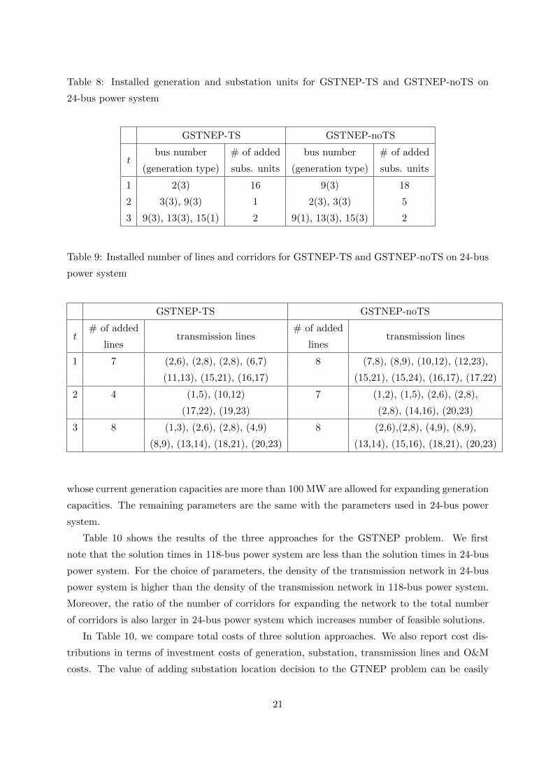
Table 8: Installed generation and substation units for GSTNEP-TS and GSTNEP-noTS on
24-bus power system
GSTNEP-TS GSTNEP-noTS
tbus number # of added bus number # of added
(generation type) subs. units (generation type) subs. units
1 2(3) 16 9(3) 18
2 3(3), 9(3) 1 2(3), 3(3) 5
3 9(3), 13(3), 15(1) 2 9(1), 13(3), 15(3) 2
Table 9: Installed number of lines and corridors for GSTNEP-TS and GSTNEP-noTS on 24-bus
power system
GSTNEP-TS GSTNEP-noTS
t# of added
transmission lines# of added
transmission lineslines lines
1 7 (2,6), (2,8), (2,8), (6,7) 8 (7,8), (8,9), (10,12), (12,23),
(11,13), (15,21), (16,17) (15,21), (15,24), (16,17), (17,22)
2 4 (1,5), (10,12) 7 (1,2), (1,5), (2,6), (2,8),
(17,22), (19,23) (2,8), (14,16), (20,23)
3 8 (1,3), (2,6), (2,8), (4,9) 8 (2,6),(2,8), (4,9), (8,9),
(8,9), (13,14), (18,21), (20,23) (13,14), (15,16), (18,21), (20,23)
whose current generation capacities are more than 100 MW are allowed for expanding generation
capacities. The remaining parameters are the same with the parameters used in 24-bus power
system.
Table 10 shows the results of the three approaches for the GSTNEP problem. We first
note that the solution times in 118-bus power system are less than the solution times in 24-bus
power system. For the choice of parameters, the density of the transmission network in 24-bus
power system is higher than the density of the transmission network in 118-bus power system.
Moreover, the ratio of the number of corridors for expanding the network to the total number
of corridors is also larger in 24-bus power system which increases number of feasible solutions.
In Table 10, we compare total costs of three solution approaches. We also report cost dis-
tributions in terms of investment costs of generation, substation, transmission lines and O&M
costs. The value of adding substation location decision to the GTNEP problem can be easily
21

observed from Table 10. The investment cost of generation units in GSTNEP-L is $197.31M
higher than the investment cost of generation units in sequential approach whereas the invest-
ment cost of substations in GSTNEP-L is $565.49M less than the investment cost of substations
in sequential approach. Hence, by adding substation location decisions to the problem, the ob-
jective value is decreased by 4.28%. For 118-bus power system, GSTNEP-L finds the optimum
solution in approximately 9.3 hours whereas sequential and time-based solution approaches finds
the solution in 65 seconds and 8 minutes, respectively. Although the solution time of the sequen-
tial approach is less than the solution time of the proposed time-based solution approach, the
proposed method finds a solution that has smaller objective value than solution of the sequen-
tial approach. The gap between the solution of the time-based approach and optimal solution
is 2.77%.
Table 10: Comparison of cases GSTNEP-TS for three approaches on 118-bus power system
GSTNEP-TS
GSTNEP-L Sequential Time-based
total cost (106$) 9143.83 9535.15 9397.45
zinv (106$) 921.03 723.72 662.70
zsub(106$) 999.36 1564.85 1044.50
zline (106$) 2.56 0.43 7.81
zom (106$) 7220.85 7246.16 7682.44
gap(%) 4.28% 2.77%
5. Conclusion
In this paper, we study a multi-period long-term power expansion planning problem that in-
cludes decisions related to substations’ locations and sizes. In the literature, substation decisions
are not explicitly considered in the transmission network design problems. In this paper, we
propose a mathematical programming model for the integrated problem that finds a minimum
cost network and locations of substations and generation units. In the computational study, we
discuss the value of adding substation decisions to the problem on 24-bus power system. To
overcome computational burden of the problem, we also propose a time-based solution approach
in which we decompose the multi-period problem into single-period problems and proceed by
fixing the output of the one period in the next time periods. We conclude that this approach
provides better results than the results of sequential approach both in terms of solution quality
and solution time.
22
We also analyze the effect of TS to the GSTNEP problem and discuss the results of the
model, sequential and time-based approaches when TS is not allowed. In this case, the proposed
solution approach also provides better results than the sequential approach in terms of solution
quality. We then apply and compare the solution approaches to a larger network, 118-bus power
system. Similar to the 24-bus power system, the proposed solution approach provides better
solutions compared to solutions obtained with the sequential approach.
23
References
[1] V. Krishnan, J. Ho, B.F. Hobbs, A.L. Liu, J.D. McCalley, M. Shahidehpour, and Q.P.
Zheng. Co-optimization of electricity transmission and generation resources for planning
and policy analysis: review of concepts and modeling approaches. Energy Systems, 7(2):
297–332, 2016.
[2] E.B. Fisher, R.P. O’Neill, and M.C. Ferris. Optimal transmission switching. IEEE Trans-
actions on Power Systems, 23(3):1346–1355, 2008.
[3] K.W Hedman, M.C. Ferris, R.P. O’Neill, E.B. Fisher, and S.S. Oren. Co-optimization
of generation unit commitment and transmission switching with N-1 reliability. IEEE
Transactions on Power Systems, 25(2):1052–1063, 2010.
[4] R. Albert, I. Albert, and G.L. Nakarado. Structural vulnerability of the North American
power grid. Physical Review E, 69(2):025103, 2004.
[5] M.S. Sepasian, H. Seifi, A.A. Foroud, and A.R. Hatami. A multiyear security constrained
hybrid generation-transmission expansion planning algorithm including fuel supply costs.
IEEE Transactions on Power Systems, 24(3):1609–1618, 2009.
[6] P.R.V. Horne, L.L. Garver, and A.E. Miscally. Transmission plans impacted by generation
siting a new study method. IEEE Trans. Power Appa. Syst., (5):2563–2567, 1981.
[7] H.M.D.R.H. Samarakoon, R.M. Shrestha, and O. Fujiwara. A mixed integer linear pro-
gramming model for transmission expansion planning with generation location selection.
Int. J. Electr. Power Energy Syst., 23(4):285–293, 2001.
[8] B. Alizadeh and S. Jadid. Reliability constrained coordination of generation and transmis-
sion expansion planning in power systems using mixed integer programming. IET Gener.
Transm. Distrib., 5(9):948–960, 2011.
[9] B. Alizadeh and S. Jadid. A dynamic model for coordination of generation and transmission
expansion planning in power systems. Int. J. Electr. Power Energy Syst., 65:408–418, 2015.
[10] M. Jenabi, S.M.T.F. Ghomi, S.A. Torabi, and S.H. Hosseinian. A Benders decomposition
algorithm for a multi-area, multi-stage integrated resource planning in power systems. J.
Oper. Res. Society, 64(8):1118–1136, 2012.
[11] O.J. Guerra, D.A. Tejada, and G.V. Reklaitis. An optimization framework for the integrated
planning of generation and transmission expansion in interconnected power systems. Applied
Energy, 170:1–21, 2016.
24
[12] A.H. Seddighi and A. Ahmadi-Javid. Integrated multiperiod power generation and trans-
mission expansion planning with sustainability aspects in a stochastic environment. Energy,
86:9–18, 2015.
[13] F.D. Munoz, B.F. Hobbs, and J.-P. Watson. New bounding and decomposition approaches
for MILP investment problems: Multi-area transmission and generation planning under
policy constraints. European Journal of Operational Research, 248(3):888–898, 2016.
[14] R. Mınguez and R. Garcıa-Bertrand. Robust transmission network expansion planning in
energy systems: Improving computational performance. European Journal of Operational
Research, 248(1):21–32, 2016.
[15] V. Grimm, A. Martin, M. Schmidt, M. Weibelzahl, and G. Zottl. Transmission and gen-
eration investment in electricity markets: The effects of market splitting and network fee
regimes. European Journal of Operational Research, 254(2):493–509, 2016.
[16] M.E. Cebeci, S. Eren, O.B. Tor, and N. Guven. Transmission and substation expansion
planning using mixed integer programming. In North American Power Symposium (NAPS),
2011, pages 1–5. IEEE, 2011.
[17] T. Akbari, M. Heidarizadeh, M.A. Siab, and M. Abroshan. Towards integrated planning:
Simultaneous transmission and substation expansion planning. Electric Power Syst. Res.,
86:131–139, 2012.
[18] A. Khodaei, M. Shahidehpour, and S. Kamalinia. Transmission switching in expansion
planning. IEEE Transactions on Power Systems, 25(3):1722–1733, 2010.
[19] J.C. Villumsen and A.B. Philpott. Investment in electricity networks with transmission
switching. European Journal of Operational Research, 222(2):377–385, 2012.
[20] S. Dehghan and N. Amjady. Robust transmission and energy storage expansion planning in
wind farm-integrated power systems considering transmission switching. IEEE Transactions
on Sustainable Energy, 7(2):765–774, 2016.
[21] L. Baringo and A.J. Conejo. Correlated wind-power production and electric load scenarios
for investment decisions. Applied energy, 101:475–482, 2013.
[22] A. Tabares, J.F. Franco, M. Lavorato, and M.J. Rider. Multistage long-term expansion
planning of electrical distribution systems considering multiple alternatives. IEEE Trans-
actions on Power Systems, 31(3):1900–1914, 2016.
[23] L. Bahiense, G.C. Oliveira, M. Pereira, and S. Granville. A mixed integer disjunctive model
for transmission network expansion. IEEE Trans. Power Syst., 16(3):560–565, 2001.
25
[24] IEEE reliability test system. IEEE Trans Power Appar Syst, 98(6):2047–2054, 1979.
[25] A.S. Kocaman, C. Abad, T.J. Troy, W.T. Huh, and V. Modi. A stochastic model for a
macroscale hybrid renewable energy system. Renewable and Sustainable Energy Rev., 54:
688–703, 2016.
[26] N. Alguacil, A.L. Motto, and A.J. Conejo. Transmission expansion planning: a mixed-
integer LP approach. IEEE Transactions on Power Systems, 18(3):1070–1077, 2003.
[27] Risheng Fang and David J Hill. A new strategy for transmission expansion in competitive
electricity markets. IEEE Transactions on power systems, 18(1):374–380, 2003.
[28] International Electrotechnical Commission. Efficient electrical energy transmission and
distribution. Report, Switzerland, 2007.
[29] TEIAS. 2015 yılı yatırım programı, 2015. URL http://www.teias.gov.tr/
Yatirimlar.aspx. [Accessed 7 April 2017].
[30] IEEE 118 bus system, . URL http://motor.ece.iit.edu/data/Data 118 Bus.pdf. [Ac-
cessed 7 April 2017].
[31] IEEE 118 bus system, . URL http://motor.ece.iit.edu/data/118 UMP.xls. [Accessed
7 April 2017].
26


![July 2012 Buchanan Creek Substation Transmission Project Creek... · Buchanan Creek Substation Transmission Project 1 ... new substation and approximately 150 metres of new ... (kV)],](https://static.fdocuments.in/doc/165x107/5ae59a7b7f8b9ae1578c809f/july-2012-buchanan-creek-substation-transmission-creekbuchanan-creek-substation.jpg)