subordination and convolution of analytic, meromorphic and ...
197
SUBORDINATION AND CONVOLUTION OF ANALYTIC, MEROMORPHIC AND HARMONIC FUNCTIONS CHANDRASHEKAR A/L RAMASAMY UNIVERSITI SAINS MALAYSIA 2012
Transcript of subordination and convolution of analytic, meromorphic and ...

SUBORDINATION AND CONVOLUTION OF
ANALYTIC, MEROMORPHIC AND HARMONIC
FUNCTIONS
CHANDRASHEKAR A/L RAMASAMY
UNIVERSITI SAINS MALAYSIA
2012
SUBORDINATION AND CONVOLUTION OF
ANALYTIC, MEROMORPHIC AND HARMONIC
FUNCTIONS
by
CHANDRASHEKAR A/L RAMASAMY
Thesis submitted in fulfilment of the requirements for the Degree ofDoctor of Philosophy in Mathematics
July 2012

ACKNOWLEDGEMENT
There are many people that I have to acknowledge and thank for all their help
and support during this research effort.
First and foremost, I sincerely acknowledge and am indebted to my main
supervisor, Dr. Lee See Keong for his continued support, motivation, guidance,
supervision and help throughout my research.
I would like to express my special thanks to the head of the Research Group in
Geometric Function Theory, Universiti Sains Malaysia (USM), Prof. Dato’ Rosihan
M. Ali, for his valuable suggestions, encouragement and guidance throughout my
research. I also deeply appreciate his financial assistance for this research through
generous grants, which supported my attending overseas conference and my living
expenses during the term of my study.
I gratefully acknowledge my field supervisior Prof. V. Ravichandran for his
guidance and advice during the progress of this work, particularly in the theory of
convolution, subordination and superordination. Another person who deserves my
sincere gratitude is my co-supervisor, Prof. K. G. Subramanian (currently in the
School of Computer Sciences, USM) for his assistance, encouragement and support
in carrying out my research especially in harmonic functions.
My gratitude also goes to Assist. Prof. A. Swaminathan, Assoc. Prof. B. Adolf
Stephen, Prof. S. Ponnusamy, Prof. Yusuf Abu Muhanna and Prof. Zayid Abdul-
hadi for their help and ideas in my studies.
I am thankful to the Dean of School of Mathematical Sciences, Prof. Ahmad
Izani Md. Ismail, and the entire staff of the School of Mathematical Sciences,
ii
USM, for the facilities and supports provided during my study.
I wish to express my gratitude to Universiti Sains Malaysia for granting me
USM Fellowship through Institute of Postgraduate Studies (IPS) to support my
studies at USM.
Not forgetting, my heartfelt thanks go to all my family members especially my
parents and Dr. Seetha, who have been very supportive during my study.
Last but not in the least, I would like to thank some good samaritans and
colleagues, Mr. Subra, ASP. Saralanathan, ASP. Subramaniam, Dr. Raja, Dr. Ve-
jayakumaran, Mrs. Shamani, Mrs. Maisarah, Dr. Abeer, Mrs. Mahnaz, Dr. Saiful,
Dr. Wong Voon Hee, Mr. Sara, Mr. Guna, Mr. Tisu and Mr. Suren who had helped
and encouraged me during my research work.
iii

TABLE OF CONTENTS
Page
ACKNOWLEDGMENT ii
TABLE OF CONTENTS iv
SYMBOLS vi
ABSTRAK xiv
ABSTRACT xvi
CHAPTER
1 INTRODUCTION 11.1 Univalent Functions 11.2 Differential Subordination and Differential Superordination 151.3 Convolution and Hypergeometric Functions 17
1.3.1 Convolution 171.3.2 Hypergeometric Functions 18
1.4 Meromorphic Functions 231.5 Harmonic Functions 251.6 Scope of the Thesis 29
2 PRELIMINARY RESULTS 312.1 Differential Subordination and Differential Superordination 312.2 Convolution 332.3 Hypergeometric Functions 34
3 CONVOLUTIONS OF MEROMORPHIC MULTIVALENT FUNC-TIONS WITH RESPECT TO N-PLY POINTS AND SYMMET-RIC CONJUGATE POINTS 363.1 Introduction 363.2 Functions with Respect to n-ply Points 413.3 Functions with Respect to n-ply Symmetric Points 523.4 Functions with Respect to n-ply Conjugate Points 553.5 Functions with Respect to n-ply Symmetric Conjugate Points 59
4 DIFFERENTIAL SANDWICH RESULTS FOR MULTIVALENTFUNCTIONS 624.1 Introduction 624.2 Subordination of the Dziok-Srivastava Operator 634.3 Superordination of the Dziok-Srivastava Operator 84
iv

4.4 Subordination of the Liu-Srivastava Operator 914.5 Superordination of the Liu-Srivastava Operator 102
5 HALF-PLANE DIFFERENTIAL SUBORDINATION CHAIN 1085.1 Introduction 1085.2 Some Subordination Results 1115.3 Sufficient Conditions for Starlikeness 122
6 HARMONIC FUNCTIONS ASSOCIATED WITH HYPERGE-OMETRIC FUNCTIONS 1396.1 Introduction 1396.2 Coefficient Condition for Gaussian Hypergeometric Function 1436.3 Integral Operators 1496.4 Coefficient Conditions for Incomplete Beta Function 1516.5 Coefficient Condition for Dziok-Srivastava Operator 1536.6 Extreme Points and Inclusion Results 158
CONCLUSION 163
BIBLIOGRAPHY 164
PUBLICATIONS 179
v

SYMBOLS
Symbol Description Page
Ap Class of all p-valent analytic functions f of the form 2
f(z) = zp +∑∞k=p+1 akz
k (z ∈ D)
A A1 2
(a)n Pochhammer symbol defined by 18
(a)n :=
1, n = 0;
a(a+ 1)(a+ 2) . . . (a+ n− 1), n ∈ N.
arg Argument of a complex number 4
C Complex plane 1
CS(α)f ∈ A : zf ′ ∈ SS(α)
44
CC Class of close-to-convex functions in A 6
CCn(h)f ∈ A :
zf ′(z)φn(z)
≺ h(z), φ ∈ ST n(h),φn(z)z 6= 0 in D
38
CCng (h) f ∈ A : f ∗ g ∈ CCn(h) 38
co(D) The closed convex hull of a set D 34
CV Class of convex functions in A 4
CV(α) Class of convex functions of order α in A 5
CV [A,B]f ∈ A : 1 +
zf ′′(z)f ′(z) ∈ P [A,B]
12
CV(ϕ)f ∈ A : 1 +
zf ′′(z)f ′(z) ≺ ϕ(z)
14
CVH , CV0H Classes of harmonic convex functions 27
CVn(h)f ∈ A :
(zf ′)′(z)f ′n(z)
≺ h(z), f ′n(z) 6= 0 in D
37
vi
CVng (h) f ∈ A : f ∗ g ∈ CVn(h) 37
CVCn(h)
f ∈ A :
2(zf ′)′(z)f ′n(z)+f ′n(z)
≺ h(z), f ′n(z) + f ′n(z) 6= 0 in D
40
CVCng (h) f ∈ A : f ∗ g ∈ CVCn(h) 40
CVSn(h)f ∈ A :
2(zf ′)′(z)f ′n(z)+f ′n(−z) ≺ h(z), f ′n(z) + f ′n(−z) 6= 0 in D
39
CVSng (h) f ∈ A : f ∗ g ∈ CVSn(h) 39
CVSCn(h)
f ∈ A :
2(zf ′)′(z)f ′n(z)+f ′n(−z)
≺ h(z), f ′n(z) + f ′n(−z) 6= 0 in D
40
CVSCng (h) f ∈ A : f ∗ g ∈ CVSCn(h) 40
D Open unit disk z ∈ C : |z| < 1 1
D Closed unit disk z ∈ C : |z| ≤ 1 31
D∗ Open punctured unit disk z ∈ C : 0 < |z| < 1 23
∂D Boundary of unit disk D 31
Dλ Ruscheweyh derivative operator 22
E(q)
ζ ∈ ∂D : lim
z→ζq(z) =∞
31
f ∗ g Convolution or Hadamard product of functions f and g 17
F(α, β, γ) Hohlov linear operator 22
F (a, b, c; z) Gaussian hypergeometric function 19
Fµ Bernardi integral operator 108
lFm Generalized hypergeometric function 20
Gbf ∈ A :
∣∣∣(1 +zf ′′(z)f ′(z)
)(f(z)zf ′(z)
)− 1∣∣∣ < b, (0 < b ≤ 1)
109
GH([α1], γ) Subclass of all starlike harmonic functions f ∈ SH 141
H(D) Class of all analytic functions in D 2
H[a, n] Class of all analytic functions f in D of the form 2
vii
f(z) = a+ anzn + an+1z
n+1 + · · ·
H0 := H[0, 1] Class of analytic functions f in D of the form 2
f(z) = a1z + a2z2 + · · ·
H := H[1, 1] Class of analytic functions f in D of the form 2
f(z) = 1 + a1z + a2z2 + · · ·
Hl,mp [α1] Dziok-Srivastava linear operator with respect to α1 ??
Hl,mp [β1] Dziok-Srivastava linear operator with respect to β1 62
H∗l,mp [β1] Liu-Srivastava linear operator 24
HP (α, β) f = h+ g ∈ SH : 140
Re(αz(h′′(z) + g′′(z)) + (h′(z) + g′(z))
)> β
HT (α, β) f ∈ SH : HP (α, β)
⋂TH 140
Im Imaginary part of a complex number 10
Jf (z) Jacobian of the function f = u+ iv 26
k Koebe function k(z) = z/(1− z)2 2
k0 Harmonic Koebe function 28
k0(z) =z−1
2z2+1
6z3
(1−z)3 +12z
2+16z
3
(1−z)3
L(α, γ) Carlson and Shaffer linear operator 22
Mp Class of all meromorphic p-valent functions f of the form 41
f(z) = 1zp +
∑∞k=1−p akz
k (p ≥ 1, z ∈ D∗)
M M1 41
MCCnp (h)f ∈Mp : −1
pzf ′(z)φn(z)
≺ h(z), 48
viii
φ ∈MST np (h), φn(z) 6= 0 in D∗
MCCnp (g, h)f ∈Mp : f ∗ g ∈MCCnp (h)
48
MCVnp (h)f ∈Mp : −1
p(zf ′(z))′
f ′n(z)≺ h(z), f ′n(z) 6= 0 in D∗
43
MCVnp (g, h)f ∈Mp : f ∗ g ∈MCVnp (h)
43
MCVCnp (h)
f ∈Mp : −1
p2(zf ′)′(z)f ′n(z)+f ′n(z)
≺ h(z), f ′n(z) + f ′n(z) 6= 0 in D∗
56
MCVCnp (g, h)f ∈Mp : f ∗ g ∈MCVCnp (h)
56
MCVSnp (h)
f ∈Mp : −1
p2(zf ′)′(z)
f ′n(z)+f ′n(−z) ≺ h(z), 52
f ′n(z) + f ′n(−z) 6= 0 in D∗
MCVSnp (g, h)f ∈Mp : f ∗ g ∈MCVSnp (h)
52
MCVSCnp (h)
f ∈Mp : −1
p2(zf ′)′(z)
f ′n(z)+f ′n(−z)≺ h(z), 59
f ′n(z) + f ′n(−z) 6= 0 in D∗
MCVSCnp (g, h)f ∈Mp : f ∗ g ∈MCVSCnp (h)
59
MOCα Class of α-convex functions in A 6
MQCnp (h)f ∈Mp : −1
p(zf ′(z))′
ϕ′n(z)≺ h(z), 49
φ ∈MCVnp (h), ϕ′n(z) 6= 0 in D∗
MQCnp (g, h)f ∈Mp : f ∗ g ∈MQCnp (h)
49
MST p(α)f ∈Mp : −Re 1
pzf ′(z)f(z)
> α (0 ≤ α < 1)
42
MST p(h)f ∈Mp : −1
pzf ′(z)f(z)
≺ h(z)
43
MST p(g, h)f ∈Mp : f ∗ g ∈MST p(h)
42
MST np (h)f ∈Mp : −1
pzf ′(z)fn(z)
≺ h(z), fn(z) 6= 0 in D∗
43
MST np (g, h)f ∈Mp : f ∗ g ∈MST np (h)
43
MST Cnp (h)
f ∈Mp : −1
p2zf ′(z)
fn(z)+fn(z)≺ h(z), fn(z) + fn(z) 6= 0 in D∗
55
ix

MST Cnp (g, h)f ∈Mp : f ∗ g ∈MST Cnp (h)
55
MST Snp (h)f ∈Mp : −1
p2zf ′(z)
fn(z)−fn(−z) ≺ h(z), 52
fn(z)− fn(−z) 6= 0 in D∗
MST Snp (g, h)f ∈Mp : f ∗ g ∈MST Snp (h)
52
MST SCnp (h)
f ∈Mp : −1
p2zf ′(z)
fn(z)−fn(−z)≺ h(z), 59
fn(z)− fn(−z) 6= 0 in D∗
MST SCnp (g, h)f ∈Mp : f ∗ g ∈MST SCnp (h)
59
N 1, 2, 3, . . . 23
N0 N⋃0 23
P p ∈ H : with Re p(z) > 0, z ∈ D 11
P(α) p ∈ H : with Re p(z) > α, z ∈ D 11
P [A,B]p ∈ H : p(z) ≺ 1+Az
1+Bz , (−1 ≤ B < A ≤ 1)
12
Q Set of all functions q(z) that analytic and injective 31
on D \ E(q) such that q′(ζ) 6= 0 for ζ ∈ ∂D \ E(q)
Q0 q ∈ Q : q(0) = 0 31
Q1 q ∈ Q : q(0) = 1 31
QC Class of quasi-convex functions in A 7
QCn(h)f ∈ A :
(zf ′)′(z)φ′n(z)
≺ h(z), φ ∈ CVn(h), φ′n(z) 6= 0 in D
38
QCng (h) f ∈ A : f ∗ g ∈ QCn(h) 38
R Set of all real numbers 2
Rα Class of prestarlike functions of order α in A 34
R[A,B]f ∈ A : f ′(z) ≺ 1+Az
1+Bz , (−1 ≤ B < A ≤ 1)
108
x

R[α] R[α,−α] 108
Re Real part of a complex number 5
S Class of all normalized univalent functions f in A 2
SH Class of all sense-preserving harmonic functions f of 26
the form f(z) = z +∑∞k=2 akz
k +∑∞k=1 bkz
k (z ∈ D)
S0H Class of all sense-preserving harmonic fucntions f of 27
the form f(z) = z +∑∞k=2 akz
k +∑∞k=2 bkz
k (z ∈ D)
Sp Class of parabolic starlike functions in A 9
Sp(α, β) Class of parabolic β-starlike functions of order α in A 10
S∗C(h)
f ∈ A :
2zf ′(z)f(z)+f(z)
≺ h(z)
36
S∗S(α)f ∈ A : Re
(zf ′(z)
f(z)−f(−z)
)> α (0 ≤ α < 1/2)
44
S∗S(h)f ∈ A :
2zf ′(z)f(z)−f(−z) ≺ h(z)
36
S∗SC(h)
f ∈ A :
2zf ′(z)f(z)−f(−z)
≺ h(z)
37
SCCα Class of strongly close-to-convex functions of order α in A 8
SCVα Class of strongly convex functions of order α in A 8
SST α Class of strongly starlike functions of order α in A 8
ST Class of starlike functions in A 5
ST (α) Class of starlike functions of order α in A 5
ST [A,B]f ∈ A :
zf ′(z)f(z)
∈ P [A,B]
12
ST (ϕ)f ∈ A :
zf ′(z)f(z)
≺ ϕ(z)
14
ST H , ST 0H Class of harmonic starlike functions 27,28
ST s Class of starlike functions with respect to 7
xi

symmetric points in A
ST c Class of starlike functions with respect to 8
conjugate points in A
ST sc Class of starlike functions with respect to 8
symmetric conjugate points in A
ST n(h)f ∈ A :
zf ′(z)fn(z)
≺ h(z), fn(z)/z 6= 0 in D
37
ST ng (h) f ∈ A : f ∗ g ∈ ST n(h) 37
ST Cn(h)
f ∈ A :
2zf ′(z)fn(z)+fn(z)
≺ h(z),fn(z)+fn(z)
z 6= 0 in D
39
ST Cng (h) f ∈ A : f ∗ g ∈ ST Cn(h) 39
ST Sn(h)f ∈ A :
2zf ′(z)fn(z)−fn(−z) ≺ h(z),
fn(z)−fn(−z)z 6= 0 in D
39
ST Sng (h) f ∈ A : f ∗ g ∈ ST Sn(h) 39
ST SCn(h)
f ∈ A :
2zf ′(z)fn(z)−fn(−z) ≺ h(z),
fn(z)−fn(−z)z 6= 0 in D
40
ST SCng (h) f ∈ A : f ∗ g ∈ ST SCn(h) 40
TH Class of all sense-preserving harmonic mappings f of 140
with negative coefficient
TH([α1], γ) f ∈ SH : GH([α1], γ)⋂TH 141
T CV0H
f ∈ S0
H : CV0H
⋂TH
29
T ST 0H
f ∈ S0
H : ST 0H
⋂TH
29
UCV Class of uniformly convex functions in A 9
UCV(α, β) Class of uniformly β-convex functions of order α in A 10
UST Class of uniformly starlike functions in A 9
≺ Subordinate to 11
xii

Ψn[Ω, q] Class of admissible functions for differential subordination 31
Ψ′n[Ω, q] Class of admissible functions for differential superordination 32
Φ(a, c; z) Confluent hypergeometric functions 19
Γ(a) Gamma function 32
Ωλ Fractional derivative operator 23
xiii
SUBORDINASI DAN KONVOLUSI FUNGSI ANALISIS, FUNGSIMEROMORFI DAN FUNGSI HARMONIK
ABSTRAK
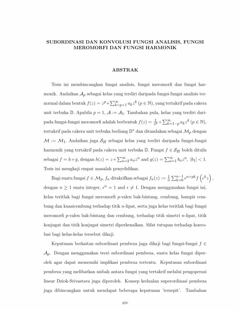
Tesis ini membincangkan fungsi analisis, fungsi meromorfi dan fungsi har-
monik. Andaikan Ap sebagai kelas yang terdiri daripada fungsi-fungsi analisis ter-
normal dalam bentuk f(z) = zp+∑∞k=p+1 akz
k (p ∈ N), yang tertakrif pada cakera
unit terbuka D. Apabila p = 1, A := A1. Tambahan pula, kelas yang terdiri dari-
pada fungsi-fungsi meromorfi adalah berbentuk f(z) = 1zp +
∑∞k=1−p akz
k (p ∈ N),
tertakrif pada cakera unit terbuka berliang D∗ dan ditandakan sebagaiMp dengan
M := M1. Andaikan juga SH sebagai kelas yang terdiri daripada fungsi-fungsi
harmonik yang tertakrif pada cakera unit terbuka D. Fungsi f ∈ SH boleh ditulis
sebagai f = h+ g, dengan h(z) = z+∑∞n=2 anz
n and g(z) =∑∞n=1 bnz
n, |b1| < 1.
Tesis ini mengkaji empat masalah penyelidikan.
Bagi suatu fungsi f ∈Mp, fn ditakrifkan sebagai fn(z) := 1n
∑n−1k=0 ε
n+pkf(εkz),
dengan n ≥ 1 suatu integer, εn = 1 and ε 6= 1. Dengan menggunakan fungsi ini,
kelas teritlak bagi fungsi meromorfi p-valen bak-bintang, cembung, hampir cem-
bung dan kuasicembung terhadap titik n-lipat, serta juga kelas teritlak bagi fungsi
meromorfi p-valen bak-bintang dan cembung, terhadap titik simetri n-lipat, titik
konjugat dan titik konjugat simetri diperkenalkan. Sifat tutupan terhadap konvo-
lusi bagi kelas-kelas tersebut dikaji.
Keputusan berkaitan subordinasi pembeza juga dikaji bagi fungsi-fungsi f ∈
Ap. Dengan menggunakan teori subordinasi pembeza, suatu kelas fungsi diper-
oleh agar dapat memenuhi implikasi pembeza tertentu. Keputusan subordinasi
pembeza yang melibatkan nisbah antara fungsi yang tertakrif melalui pengoperasi
linear Dziok-Srivastava juga diperoleh. Konsep kedualan superordinasi pembeza
juga dibincangkan untuk mendapat beberapa keputusan ’tersepit’. Tambahan
xiv
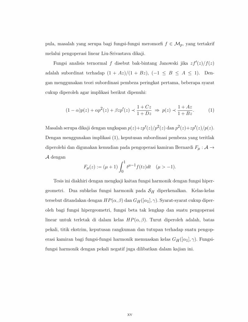
pula, masalah yang serupa bagi fungsi-fungsi meromorfi f ∈ Mp, yang tertakrif
melalui pengoperasi linear Liu-Srivastava dikaji.
Fungsi analisis ternormal f disebut bak-bintang Janowski jika zf ′(z)/f(z)
adalah subordinat terhadap (1 + Az)/(1 + Bz), (−1 ≤ B ≤ A ≤ 1). Den-
gan menggunakan teori subordinasi pembeza peringkat pertama, beberapa syarat
cukup diperoleh agar implikasi berikut dipenuhi:
(1− α)p(z) + αp2(z) + βzp′(z) ≺ 1 + Cz
1 +Dz⇒ p(z) ≺ 1 + Az
1 +Bz. (1)
Masalah serupa dikaji dengan ungkapan p(z)+zp′(z)/p2(z) dan p2(z)+zp′(z)/p(z).
Dengan menggunakan implikasi (1), keputusan subordinasi pembeza yang teritlak
diperolehi dan digunakan kemudian pada pengoperasi kamiran Bernardi Fµ : A →
A dengan
Fµ(z) := (µ+ 1)
∫ 1
0tµ−1f(tz)dt (µ > −1).
Tesis ini diakhiri dengan mengkaji kaitan fungsi harmonik dengan fungsi hiper-
geometri. Dua subkelas fungsi harmonik pada SH diperkenalkan. Kelas-kelas
tersebut ditandakan dengan HP (α, β) dan GH([α1], γ). Syarat-syarat cukup diper-
oleh bagi fungsi hipergeometri, fungsi beta tak lengkap dan suatu pengoperasi
linear untuk terletak di dalam kelas HP (α, β). Turut diperoleh adalah, batas
pekali, titik ekstrim, keputusan rangkuman dan tutupan terhadap suatu pengop-
erasi kamiran bagi fungsi-fungsi harmonik memuaskan kelas GH([α1], γ). Fungsi-
fungsi harmonik dengan pekali negatif juga dilibatkan dalam kajian ini.
xv
SUBORDINATION AND CONVOLUTION OF ANALYTIC,MEROMORPHIC AND HARMONIC FUNCTIONS
ABSTRACT
This thesis deals with analytic, meromorphic and harmonic functions. Let
Ap denote the class of normalized analytic functions of the form f(z) = zp +∑∞k=p+1 akz
k (p ∈ N), defined on the open unit disk D where p is a fixed positive
integer. When p = 1, A := A1. Further, the class of all meromorphic functions are
of the form f(z) = 1zp +
∑∞k=1−p akz
k (p ∈ N), defined in the punctured open unit
disk D∗ and denoted byMp withM :=M1. Also, let SH denote the class of sense-
preserving harmonic functions defined in the unit disk D. A function f ∈ SH can be
written as f = h+g where h(z) = z+∑∞n=2 anz
n and g(z) =∑∞n=1 bnz
n, |b1| < 1.
Four research problems are discussed in this work.
Given a function f ∈Mp, let fn be defined by fn(z) := 1n
∑n−1k=0 ε
n+pkf(εkz),
where n ≥ 1 is any integer, εn = 1 and ε 6= 1. Using this function, general classes of
meromorphic functions that are starlike, convex, close-to-convex and quasi-convex
with respect to n-ply points, as well as meromorphic functions that are starlike
and convex with respect to n-ply symmetric points, conjugate points and symmet-
ric conjugate points are introduced. Closure properties under convolution of these
classes are obtained.
Results associated with differential subordination are also investigated for func-
tions f ∈ Ap. By using the theory of differential subordination, a class of functions
is determined to satisfy certain differential implication. Differential subordination
results involving the ratios of functions defined through the Dziok-Srivastava linear
operator are also obtained. The dual concept of differential superordination is also
considered to obtain sandwich type results. Further, similar problems for mero-
morphic functions f ∈Mp, defined through the Liu-Srivastava linear operator are
xvi
investigated.
A normalized analytic function f is Janowski starlike if zf ′(z)/f(z) is subor-
dinated to (1 + Az)/(1 + Bz), (−1 ≤ B ≤ A ≤ 1). By making use of the theory
of first-order differential subordination, sufficient conditions are obtained for the
following implication to hold:
(1− α)p(z) + αp2(z) + βzp′(z) ≺ 1 + Cz
1 +Dz⇒ p(z) ≺ 1 + Az
1 +Bz. (2)
Similar problem is also investigated with the expressions p(z) + zp′(z)/p2(z) and
p2(z) + zp′(z)/p(z). Using the implication (2), a more general differential subordi-
nation result is obtained which is next applied to the Bernardi’s integral operator
Fµ : A → A given by
Fµ(z) := (µ+ 1)
∫ 1
0tµ−1f(tz)dt (µ > −1).
Finally, connections between harmonic functions and hypergeometric functions
are investigated. Two subclasses of SH are introduced. These classes are denoted
by HP (α, β) and GH([α1], γ). Sufficient conditions are obtained for a hypergeo-
metric function, an incomplete beta functions and an integral operator to be in
the class HP (α, β). Further, coefficient bounds, extreme points, inclusion results
and closure under an integral operator are also investigated for harmonic functions
satisfying the class GH([α1], γ). Harmonic functions with negative coefficients are
also considered in this investigation.
xvii

CHAPTER 1
INTRODUCTION
1.1 Univalent Functions
Geometric function theory is a branch of complex analysis which deals with the
geometric properties of analytic functions. The theory of univalent functions deals
with one-to-one analytic, meromorphic and harmonic functions.
Let C be the complex plane and D := z ∈ C : |z| < 1 be the open unit disk
in C. Let Ω be an open subset of C. Let f : Ω → C. The function f is analytic
at z0 ∈ Ω if it is differentiable at every point in some neighborhood of z0 and
it is analytic on Ω if it is analytic at all points in Ω. The analytic function f is
univalent (Schlicht) in Ω, if it takes different points in Ω to different values, that is
for any two distinct points z1 and z2 in Ω, f(z1) 6= f(z2). The function f is locally
univalent at a point z0 ∈ Ω, if it is univalent in some neighborhood of z0. For an
analytic function f, the condition f ′(z0) 6= 0 is equivalent to local univalence at z0.
The restriction of one-to-oneness (injectivity) on functions defined on Ω provides
a lot of information on the geometric and analytic properties of such functions.
We now recall the famous Riemann mapping theorem which states that, in
any simply connected domain (a domain without any holes) Ω which is not the
whole complex plane C, there exists an analytic univalent function ϕ that maps Ω
onto the unit disk.
Theorem 1.1 (Riemann Mapping Theorem) [35, p. 11] Let Ω be a simply con-
nected domain which is a proper subset of the complex plane. Let ζ be a given point
in Ω. Then there is a unique univalent analytic function f which maps Ω onto the
unit disk D satisfying f(ζ) = 0 and f ′(ζ) > 0.
In view of this, the study of analytic univalent functions on a simply connected
domain can be restricted to the study of these functions in the open unit disk D.
1

Let H(D) be the class of functions analytic in D. Let H[a, n] be the subclass
of H(D) consisting of functions of the form
f(z) = a+ anzn + an+1z
n+1 + · · ·
and let H0 ≡ H[0, 1] and H ≡ H[1, 1]. The open mapping theorem for a non-
constant analytic function shows that the derivative of a univalent function can
never vanish. Also translations and dilatations do not affect univalency. This
enables us to consider functions f that are normalized by the conditions f(0) =
0, f ′(0) = 1. Let A denote the class of such analytic functions f in D. A function
f ∈ A has the power series expansion of the form
f(z) = z +∞∑k=2
akzk (z ∈ D). (1.1)
More generally, let Ap denote the class of all analytic functions of the form
f(z) = zp +∞∑
k=p+1
akzk (z ∈ D, p ∈ N := 1, 2, 3, . . .). (1.2)
The subclass of A consisting of univalent functions is denoted by S. Thus S is the
class of all normalized univalent functions in D. The function k defined by
k(z) =z
(1− z)2=∞∑n=1
nzn (z ∈ D)
called the Koebe function which maps D onto the complex plane except for a slit
along the half-line (−∞,−1/4], is an example of a function in S. It plays a very
important role in the study of the class S. In fact, the Koebe function and its
rotations e−iαk(eiαz
), α ∈ R are the only extremal functions for various problem
in the study of geometric function theory.
2

In 1916, Bieberbach [28] proved that |a2| ≤ 2 for f ∈ S and that equality
holds if and only if f is a rotation of the Koebe function k. This result is known
as Bieberbach Theorem. He also conjectured that |an| ≤ n (n ≥ 2) for f ∈ S,
is generally valid. This conjecture is known as the Bieberbach’s (or coefficient)
conjecture. For the cases n = 3, and n = 4 the conjecture was proved by Lowner
[67], and Garabedian and Schiffer [41], respectively. Pederson and Schiffer [96]
proved the conjecture for n = 5. For n = 6, the conjecture was proved by Pederson
[95] and Ozawa [90], independently. Finaly, in 1985, Louis de Branges [34], proved
the Bieberbach’s conjecture (now known as de Branges Theorem) for all coefficients
n as in the following theorem:
Theorem 1.2 (de Branges Theorem) [34] If f ∈ S is of the form (1.1), then
|an| ≤ n (n ≥ 2)
with equality if and only if, f is the Koebe function k or one of its rotations.
The simple coefficient inequality |a2| ≤ 2 yields many important properties of
univalent functions. As a first application, we will state the covering theorem: if
f ∈ S, then the image of D under f contains a disk of radius 1/4.
Theorem 1.3 (Koebe One-Quarter Theorem) [35, p. 31] The range of every func-
tion f ∈ S contains the diskw ∈ C : |w| < 1
4
.
Another important consequence of the Bieberbach’s theorem is the distortion the-
orem that gives sharp upper and lower bounds for |f ′(z)|.
Theorem 1.4 (Distortion Theorem) [35, p. 32] For each f ∈ S,
1− r(1 + r)3
≤ |f ′(z)| ≤ 1 + r
(1− r)3(|z| = r < 1).
The result is sharp.
3
The distortion theorem can be applied to obtain sharp upper and lower bounds
for |f(z)|. This result is known as growth theorem.
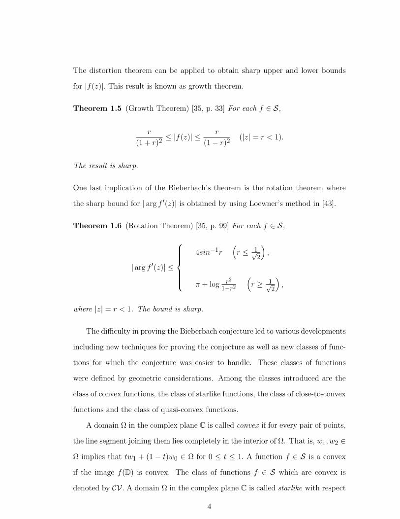
Theorem 1.5 (Growth Theorem) [35, p. 33] For each f ∈ S,
r
(1 + r)2≤ |f(z)| ≤ r
(1− r)2(|z| = r < 1).
The result is sharp.
One last implication of the Bieberbach’s theorem is the rotation theorem where
the sharp bound for | arg f ′(z)| is obtained by using Loewner’s method in [43].
Theorem 1.6 (Rotation Theorem) [35, p. 99] For each f ∈ S,
| arg f ′(z)| ≤
4sin−1r
(r ≤ 1√
2
),
π + log r2
1−r2(r ≥ 1√
2
),
where |z| = r < 1. The bound is sharp.
The difficulty in proving the Bieberbach conjecture led to various developments
including new techniques for proving the conjecture as well as new classes of func-
tions for which the conjecture was easier to handle. These classes of functions
were defined by geometric considerations. Among the classes introduced are the
class of convex functions, the class of starlike functions, the class of close-to-convex
functions and the class of quasi-convex functions.
A domain Ω in the complex plane C is called convex if for every pair of points,
the line segment joining them lies completely in the interior of Ω. That is, w1, w2 ∈
Ω implies that tw1 + (1 − t)w0 ∈ Ω for 0 ≤ t ≤ 1. A function f ∈ S is a convex
if the image f(D) is convex. The class of functions f ∈ S which are convex is
denoted by CV . A domain Ω in the complex plane C is called starlike with respect
4

to a point w0 ∈ Ω, if the line segment joining w0 to every other point w ∈ Ω lies in
the interior of Ω. In other words, for any w ∈ Ω and 0 ≤ t ≤ 1, tw0 +(1− t)w ∈ Ω.
A function f ∈ S is starlike if the image f(D) is starlike with respect to the origin.
The class of functions f ∈ S which are starlike is denoted by ST .
Analytically, a function f ∈ CV if and only if
Re
(1 +
zf ′′(z)
f ′(z)
)> 0 (z ∈ D). (1.3)
The condition (1.3) for convexity was first stated by Study [134]. Also, a function
f ∈ ST if and only if
Re
(zf ′(z)
f(z)
)> 0 (z ∈ D). (1.4)
The condition (1.4) for starlikeness is due to Nevanlinna [79]. In 1936, Robertson
[107] introduced the concepts of convex functions of order α and starlike functions
of order α, 0 ≤ α < 1. A function f ∈ S is said to be convex of order α if
Re
(1 +
zf ′′(z)
f ′(z)
)> α (z ∈ D),
and starlike of order α if
Re
(zf ′(z)
f(z)
)> α (z ∈ D).
These classes are respectively denoted by CV(α) and ST (α). Note that CV(0) =
CV and ST (0) = ST .
Every convex function is evidently starlike. Thus CV ⊂ ST ⊂ S. However,
there is a close analytic connection between convex and starlike functions. Alexan-
der [7] first observed this in 1915 and proved the following theorem.
Theorem 1.7 (Alexander’s Theorem) [35, p. 43] Let f ∈ S. Then f ∈ CV if and
only if zf ′ ∈ ST .
5
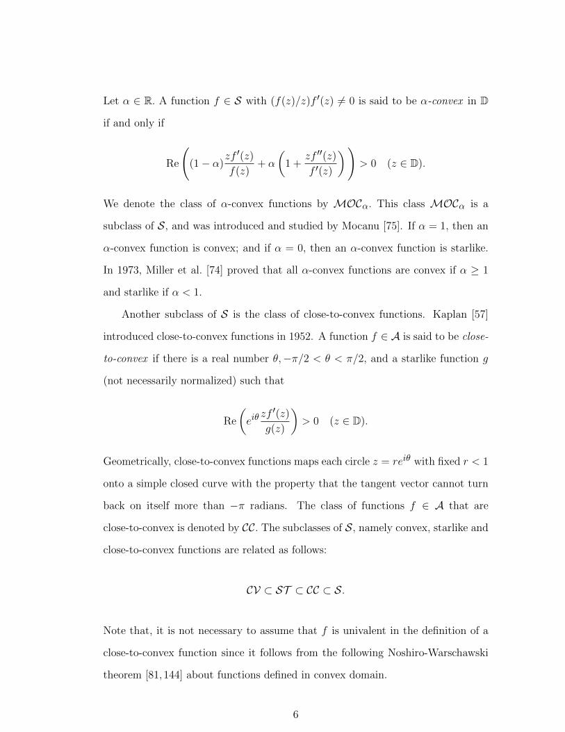
Let α ∈ R. A function f ∈ S with (f(z)/z)f ′(z) 6= 0 is said to be α-convex in D
if and only if
Re
((1− α)
zf ′(z)
f(z)+ α
(1 +
zf ′′(z)
f ′(z)
))> 0 (z ∈ D).
We denote the class of α-convex functions by MOCα. This class MOCα is a
subclass of S, and was introduced and studied by Mocanu [75]. If α = 1, then an
α-convex function is convex; and if α = 0, then an α-convex function is starlike.
In 1973, Miller et al. [74] proved that all α-convex functions are convex if α ≥ 1
and starlike if α < 1.
Another subclass of S is the class of close-to-convex functions. Kaplan [57]
introduced close-to-convex functions in 1952. A function f ∈ A is said to be close-
to-convex if there is a real number θ,−π/2 < θ < π/2, and a starlike function g
(not necessarily normalized) such that
Re
(eiθ
zf ′(z)
g(z)
)> 0 (z ∈ D).
Geometrically, close-to-convex functions maps each circle z = reiθ with fixed r < 1
onto a simple closed curve with the property that the tangent vector cannot turn
back on itself more than −π radians. The class of functions f ∈ A that are
close-to-convex is denoted by CC. The subclasses of S, namely convex, starlike and
close-to-convex functions are related as follows:
CV ⊂ ST ⊂ CC ⊂ S.
Note that, it is not necessary to assume that f is univalent in the definition of a
close-to-convex function since it follows from the following Noshiro-Warschawski
theorem [81,144] about functions defined in convex domain.
6

Theorem 1.8 If a function f is analytic in a convex domain Ω and
Re(eiθf ′(z)
)> 0 (−π/2 ≤ θ ≤ π/2)
in Ω, then f is univalent in Ω.
Kaplan [57] applied Noshiro-Warschawski theorem to prove that every close-to-
convex function is univalent.
In 1980, Noor and Thomas [82] introduced the class of quasi-convex functions.
A function f ∈ A is said to be quasi-convex if and only if
Re
((zf ′(z))′
g′(z)
)> 0 (z ∈ D)
for some g ∈ CV . The class of functions f ∈ A that are quasi-convex is denoted
by QC.
A function f ∈ A is said to be starlike with respect to symmetric points in D if
Re
(zf ′(z)
f(z)− f(−z)
)> 0 (z ∈ D). (1.5)
This class was introduced and studied in 1959 by Sakaguchi [118]. Let the class
of these functions be denoted by ST s. Geometrically, if f ∈ ST s, then for every
r < 1, the angular velocity of f(z) about the point f(−z) is positive as z traverses
the circle |z| = r in the positive direction. Further investigations into the class
of starlike functions with respect to symmetric points can be found in [31, 80,
92, 120, 138, 140–143]. El-Ashwah and Thomas [39] introduced and studied the
classes consisting of starlike functions with respect to conjugate points, and starlike
functions with respect to symmetric conjugate points defined respectively by the
7
conditions
Re
(zf ′(z)
f(z) + f(z)
)> 0 (z ∈ D) and Re
(zf ′(z)
f(z)− f(−z)
)> 0 (z ∈ D).
The classes of these functions be denoted respectively by ST c and ST sc . Geo-
metrically, if f ∈ ST c, then for every r < 1, the angular velocity of f(z) about
the point f(z) is positive as z traverses the circle |z| = r in the positive direction
and f ∈ ST sc can be described similarly.
Brannan and Kirwan [29] introduced the classes of strongly convex and strongly
starlike functions of order α. A function f ∈ A is said to be strongly convex of
order α, 0 < α ≤ 1 if it satisfies
∣∣∣∣arg
(1 +
zf ′′(z)
f ′(z)
)∣∣∣∣ < πα
2(z ∈ D).
The class of all such functions is denoted by SCVα. Similarly, a function f ∈ A is
said to be strongly starlike of order α, 0 < α ≤ 1 if it satisfies
∣∣∣∣arg
(zf ′(z)
f(z)
)∣∣∣∣ < πα
2(z ∈ D).
The class of all such functions is denoted by SST α. Since the condition Rew(z) > 0
is equivalent to | argw(z)| < π/2, we have SCV1 = CV and SST 1 = ST
Reade [106] introduced the class of strongly close-to-convex functions of order
α. A function f ∈ A is said to be strongly close-to-convex of order α, 0 < α ≤ 1 if
there is a real β and a convex function φ that satisfies
∣∣∣∣arg
(e−iβ
f ′(z)
φ′(z)
)∣∣∣∣ ≤ απ
2(z ∈ D).
The class of all such functions is denoted by SCCα. When β = 0, SCC1 = CC.
In 1991, Goodman [45,46] introduced and investigated the classes of uniformly
8

convex and uniformly starlike functions. A function f ∈ S is uniformly convex
(starlike) if for every circular arc γ contained in D with center ζ ∈ D the image
arc f(γ) is convex (starlike with respect to f(ζ)). The class of all uniformly
convex and uniformly starlike functions is denoted by UCV and UST respectively.
Analytically, f ∈ UCV if and only if
Re
(1 + (z − ζ)
f ′′(z)
f ′(z)
)≥ 0, (z 6= ζ, (z, ζ) ∈ D× D).
and f ∈ UST if and only if
Re
(f(z)− f(ζ)
(z − ζ)f ′(z)
)≥ 0 (z 6= ζ, (z, ζ) ∈ D× D).
In 1992, Ronning [109] and Ma and Minda [70] were able to give independently
a one variable characterization for the class UCV . The function f ∈ S belongs to
UCV if and only if it satisfies
Re
(1 +
zf ′′(z)
f ′(z)
)>
∣∣∣∣zf ′′(z)
f ′(z)
∣∣∣∣ (z ∈ D). (1.6)
Using this one variable characterization of the class UCV , it is easy to obtain trans-
formations which preserve the class UCV . However, a one variable characterization
of the class UST is still unavailable. In exploring the possibility of an analogous
result of Alexander’s theorem between the classes UCV and UST , Ronning [110],
introduced a subclass Sp of parabolic starlike functions. The class Sp consist func-
tions F (z) = zf ′(z), where f belongs to the class UCV . Clearly f ∈ Sp if and only
if
Re
(zf ′(z)
f(z)
)>
∣∣∣∣zf ′(z)
f(z)− 1
∣∣∣∣ (z ∈ D). (1.7)
9
In order to interpret (1.6) and (1.7) geometrically, let
ΩPAR := w ∈ C : Rew > |w − 1|.
The set ΩPAR is the interior of the parabola
(Imw)2 < 2 Rew − 1
and it is therefore symmetric with respect to the real axis and has (1/2, 0) as its
vertex. Then f ∈ UCV if and only if 1 + zf ′′(z)/f ′(z) ∈ ΩPAR and f ∈ Sp if and
only if zf ′(z)/f(z) ∈ ΩPAR.
In [108,109], Ronning introduced the classes UCV(α, β) consist of uniformly β-
convex functions of order α and Sp(α, β) consist of parabolic β-starlike functions of
order α, −1 < α ≤ 1, β ≥ 0, which generalize the classes UCV and Sp respectively.
The function f ∈ A belongs to UCV(α, β) if and only if it satisfies the condition
Re
(1 +
zf ′′(z)
f ′(z)− α
)> β
∣∣∣∣zf ′′(z)
f ′(z)
∣∣∣∣ (z ∈ D). (1.8)
Similarly, the function f ∈ A belongs to Sp(α, β) if and only if it satisfies the
condition
Re
(zf ′(z)
f(z)− α
)> β
∣∣∣∣zf ′(z)
f(z)− 1
∣∣∣∣ (z ∈ D). (1.9)
Indeed it follows from (1.9) and (1.8) that f ∈ UCV(α, β) if and only if zf ′ ∈
Sp(α, β). For −1 < α ≤ 1, β ≥ 0, let
Ωα,βPAR := w ∈ C : Rew − α > β|w − 1|.
10

The set Ωα,βPAR is the interior of the parabola
(β Imw)2 < (Rew − α)2 − β2(Rew − 1)2.
Geometrically, f ∈ UCV(α, β) if and only if 1 + zf ′′(z)/f ′(z) ∈ Ωα,βPAR and
f ∈ Sp(α, β) if and only if zf ′(z)/f(z) ∈ Ωα,βPAR. Clearly, UCV(0, 1) = UCV and
Sp(0, 1) = Sp.
Several subclasses of starlike and convex functions can be unified by using
subordination between analytic functions. An analytic function f ∈ A is subordi-
nate to an analytic function g ∈ A, denoted by f ≺ g, if there exists an analytic
function ω, with ω(0) = 0 and |ω(z)| < 1 satisfying f(z) = g(ω(z)). In particular,
if the function g ∈ S, then f ≺ g is equivalent to f(0) = g(0) and f(D) ⊂ g(D). If
f ≺ g, we say g is superordinate to f .
Let P be the class of all analytic functions p of the form
p(z) = 1 + c1z + c2z2 + · · · = 1 +
∞∑n=1
pnzn
with
Re p(z) > 0 (z ∈ D). (1.10)
Any function in P is called a Caratheodory function. More generally, for 0 ≤ α <
1, we denote by P(α) the class of analytic functions p ∈ P with
Re p(z) > α (z ∈ D).
Most of the subclasses of functions in S are in one way or other related to the
class P . For example, the function f ∈ ST if and only if zf(z)/f(z) ∈ P and the
function f ∈ CV if and only if 1 + zf ′′(z)/f ′(z) ∈ P .
11

In terms of subordination, the analytic condition (1.10) can be written as
p(z) ≺ 1 + z
1− z(z ∈ D).
This follows since the mapping q(z) = (1 + z)/(1− z) maps D onto the right-half
plane. In this light, the conditions (1.3) and (1.4) are respectively equivalent to
1 +zf ′′(z)
f ′(z)≺ 1 + z
1− z(z ∈ D) (1.11)
and
zf ′(z)
f(z)≺ 1 + z
1− z(z ∈ D). (1.12)
For |B| ≤ 1 and A 6= B, a function p, analytic in D with p(0) = 1, belongs to
the class P [A,B] if
p(z) ≺ 1 + Az
1 +Bz(z ∈ D).
In 1973, Janowski [55] introduced the class P [A,B] for −1 ≤ B < A ≤ 1. He
introduced and investigated the classes of Janowski convex and Janowski star-
like functions by replacing the function (1 + z)/(1 − z) in (1.11) and (1.12)
with (1 + Az)/(1 + Bz). The classes of Janowski convex and Janowski star-
like functions are denoted by CV [A,B] and ST [A,B] respectively. In particular
P [A,B] ⊂ P [1,−1] = P . It is also evident that, under the condition p(0) = 1
and 0 ≤ α < 1, P [1 − 2α,−1] = P(α). Thus, the classes CV [A,B] and ST [A,B]
include the classes CV and ST respectively.
Rønning [110] and Ma and Minda [70] showed that the function φPAR(z)
defined by
φPAR(z) = 1 +2
π2
(log
1 +√z
1−√z
)2
(z ∈ D)
maps D onto the parabolic region ΩPAR. Therefore the classes UCV and Sp can
12

be expressed in the form
UCV =
f ∈ A : 1 +
zf ′′(z)
f ′(z)≺ φPAR(z)
(1.13)
and
Sp =
f ∈ A :
zf ′(z)
f(z)≺ φPAR(z)
. (1.14)
Analogous to (1.13) and (1.14), the classes UCV(α, β) and Sp(α, β) were also
defined in terms of subordination in [2, 3, 93] for 0 ≤ α < 1 and β ≥ 0. Let
p(z) = 1 + zf ′′(z)/f ′(z) or p(z) = zf ′(z)/f(z). Then the conditions (1.8) or (1.9)
are rewritten in the form
p(z) ≺ qα,β(z),
where the function qα,β for β = 0 and β = 1 are
qα,0(z) =1 + (1− 2α)z
1− z, and qα,1(z) = 1 +
2(1− α)
π2
(1 +√z
1−√z
)2
.
For 0 < β < 1, the function qα,β is
qα,β(z) =1− α1− β2
cos
(2
π
(cos−1 β
)i log
1 +√z
1−√z
)− β2 − α
1− β2,
and if β > 1, then qα,β has the form
qα,β(z) =1− αβ2 − 1
sin
π
2K(β)
∫ u(z)/√β
0
dt√1− t2
√1− β2t2
+β2 − αβ2 − 1
,
where u(z) = (z −√β)/(1−
√βz) and K is such that β = cosh(πK ′(z))/4K(z)).
In an effort to unify the subclasses of univalent functions, Ma and Minda [68]
gave a unified presentation of various subclasses of starlike and convex functions.
For this purpose, let ϕ be an analytic function with positive real part in D, nor-
13

malized by the conditions ϕ(0) = 1 and ϕ(0) > 0, such that ϕ maps the unit disk
D onto a region starlike with respect to 1 that is symmetric with respect to the
real axis. They introduce the following classes
CV(ϕ) :=
f ∈ A : 1 +
zf ′′(z)
f ′(z)≺ ϕ(z)
and
ST (ϕ) :=
f ∈ A :
zf ′(z)
f(z)≺ ϕ(z)
.
These functions are called Ma-Minda convex and starlike functions respectively.
It is clear that for special choices of ϕ, these classes envelop several well-known
subclasses of univalent function as special cases. For example, when ϕA,B(z) =
(1 +Az)/(1 +Bz) where −1 ≤ B < A ≤ 1, the class ST (ϕA,B) = ST [A,B], and
the class CV(φPAR) = UCV .
Define the functions kϕ, hϕ : D→ C respectively by
1 +zk′′ϕ(z)
k′ϕ(z)= ϕ(z) (z ∈ D, kϕ ∈ A)
and
zh′ϕ(z)
hϕ(z)= ϕ(z) (z ∈ D, hϕ ∈ A).
In [68], Ma and Minda introduced the functions kϕ and hϕ in CV(ϕ) and ST (ϕ)
respectively, which turned out to be extremal for certain problems. For the class
of Ma-Minda convex functions, the following theorem is holds.
Theorem 1.9 [68] If f ∈ CV(ϕ), then, for |z| = r,
k′ϕ(−r) ≤ |f ′(z)| ≤ k′ϕ(r),
−kϕ(−r) ≤ |f(z)| ≤ kϕ(r).
14
Equality holds for some z 6= 0 if and only if f is a rotation of kϕ. Also either f is
a rotation of kϕ or f(D) contains the disk |w| ≤ −kϕ(−1), where
−kϕ(−1) = limr→1−
(−kϕ(−r)).
Further, for |z0| = r < 1,
| arg(f ′(z0))| ≤ max|z|=r
| arg k′ϕ(z)|.
Theorem 1.9 gives distortion, growth, covering and rotation results for the class
CV(ϕ). Corresponding results for functions in ST (ϕ) were also obtained by Ma and
Minda [68]. The additional assumptions min|z|=r |ϕ(z)| = |ϕ(−r)| and min|z|=r |ϕ(z)| =
|ϕ(r)| are needed in the distortion theorem for f ∈ ST (ϕ).
More information on univalent functions can be found in the books by Good-
man [44], Duren [35], Pommerenke [97], Graham and Kohr [47] and Rosenblum
and Rovnyak [111]. Certain aspects of the subject have also been covered in the
books by Nehari [78], Goluzin [42] and Hayman [50].
1.2 Differential Subordination and Differential Superordination
The theory of differential subordination and the dual theory of differential superordi-
nation were developed by Miller and Mocanu [72,73]
Let ψ(r, s, t; z) : C3×D→ C and let h be univalent in D. If p is analytic in D
and satisfies the second order differential subordination
ψ(p(z), zp′(z), z2p′′(z); z
)≺ h(z), (1.15)
then p is called a solution of the differential subordination. The univalent function
q is called a dominant of the solution of the differential subordination or more
simply dominant, if p ≺ q for all p satisfying (1.15). A dominant q1 satisfying
q1 ≺ q for all dominants q of (1.15) is said to be the best dominant of (1.15). The
15

best dominant is unique up to a rotation of D. If p(z) ∈ H[a, n], then p will be
called an (a, n)-solution, q an (a, n)-dominant, and q1 the best (a, n)-dominant.
Let Ω ⊂ C and let (1.15) be replaced by
ψ(p(z), zp′(z), z2p′′(z); z
)∈ Ω, for all z ∈ D. (1.16)
Even though this is a “differential inclusion” and ψ(p(z), zp′(z), z2p′′(z); z
)may
not be analytic in D, the condition in (1.16) will also be referred as a second order
differential subordination, and the same definition of solution, dominant and best
dominant as given above can be extended to this generalization. See [72] for more
information on differential subordination.
Let ψ(r, s, t; z) : C3 × D→ C and let h be analytic in D. If p and
ψ(p(z), zp′(z), z2p′′(z); z
)are univalent in D and satisfies the second order differential superordination
h(z) ≺ ψ(p(z), zp′(z), z2p′′(z); z
), (1.17)
then p is called a solution of the differential superordination. An analytic function
q is called a subordinant of the solution of the differential superordination or more
simply subordinant, if q ≺ p for all p satisfying (1.17). A univalent subordinant q1
satisfying q ≺ q1 for all subordinants q of (1.17) is said to be the best subordinant
of (1.17). The best subordinant is unique up to a rotation of D. Let Ω ⊂ C and
let (1.17) be replaced by
Ω ⊂ψ(p(z), zp′(z), z2p′′(z); z
)|z ∈ D
. (1.18)
Even though this more general situation is a “differential containment”, the con-
16
dition in (1.18) will also be referred as a second order differential superordination
and the definition of solution, subordinant and best subordinant can be extended
to this generalization. See [73] for more information on the differential superordi-
nation.
1.3 Convolution and Hypergeometric Functions
1.3.1 Convolution
For two analytic functions f and g given by their Taylor series f(z) = a1z +
a2z2 + a3z
3 + · · · =∑∞k=1 akz
k and g(z) = b1z + b2z2 + b3z
3 + · · · =∑∞k=1 bkz
k,
the convolution or Hadamard product, denoted by f ∗ g is defined by the analytic
function
(f ∗ g)(z) = a1b1z + a2b2z2 + a3b3z
3 + · · · =∞∑k=1
akbkzk.
The product is named after Jacques Hadamard [48] who published the first in-
depth analysis of this product in 1899. The Hadamard product is commutative
and associative. The first derivative of the product f ∗ g is related to the first
derivatives of f and g by
z(f ∗ g)′(z) =((zf)′ ∗ g
)(z) =
(f ∗ (zg)′
)(z).
The second derivative of the product is related to the first derivative of f ∗ g, f
and g by
z2(f ∗g)′′(z)+z(f ∗g)′(z) = z(z(f ∗g)′
)′(z) = z
((zf ′)∗g
)′(z) =
((zf ′)∗ (zg′)
)(z).
For any analytic function g with g(0) = 0, the function f(z) =∑∞k=1 z
n = z/(1−z)
is an identity. Hence, (f ∗ g)(z) = g(z).
17
The importance of convolution lies in the fact that many linear operators in
geometric function theory are special cases of the convolution operator f 7−→ f ∗g
for an appropriate fixed g. Polya and Schoenberg [101] conjectured that the classes
of convex functions CV and starlike fucntions ST are preserved under convolution
with convex functions. In other words, if f ∈ CV and g ∈ CV(g ∈ ST ), then
f ∗ g ∈ CV(f ∗ g ∈ ST ).
In 1973, Ruscheweyh and Sheil-Small [116] proved the Polya-Schoenberg con-
jecture. In fact, Ruscheweyh and Sheil-Small [116] prove that the class CC of
close-to-convex functions is also closed under convolution with convex functions.
They proved the following more general theorem that plays an important role in
the theory of convolutions:
Theorem 1.10 [116, p. 128] If f ∈ CV , g ∈ ST and φ ∈ P , thenf∗(φg)f∗g ∈ P .
1.3.2 Hypergeometric Functions
The exploitation of hypergeometric functions in the proof of the Bieberbach con-
jecture by Louis de Branges has given function theorists a renewed impulse to
study this special function. As a result there are a numbers of works on this
topic [20,30,69,71,99,117].
The Pochhammer symbol or ascending factorial is defined by
(a)n :=Γ(a+ n)
Γ(a)=
1, (n = 0);
a(a+ 1)(a+ 2) . . . (a+ n− 1), (n ∈ N)
(1.19)
where Γ(a), denotes the Gamma function.
It is well known that the functions f(z) = (1− z)−1 and g(z) = (1− z)−a can
18

be represented as in the following geometric series :
(1− z)−1 =∞∑k=0
zk. (1.20)
(1− z)−a =∞∑k=0
(−a
k
)(−z)k =
∞∑k=0
(a)kk!
zk. (1.21)
The geometric series representations (1.20) and (1.21) lead to the consideration of
the function defined by
Φ(a, c; z) = 1 +a
c
z
1!+a(a+ 1)
c(c+ 1)
z2
2!+a(a+ 1)(a+ 2)
c(c+ 1)(c+ 2)
z3
3!+ · · · . (1.22)
where a, c ∈ C with c 6= 0,−1,−2 · · · . This function, called a confluent (or Kum-
mer) hypergeometric function, satisfies Kummer’s differential equation
zw′′(z) + (c− z)w′(z)− aw(z) = 0.
By using (1.19), (1.22) can be written in the form
Φ(a, c; z) =∞∑k=0
(a)k(c)k
zk
k !=
Γ(c)
Γ(a)
∞∑k=0
Γ(a+ k)
Γ(c+ k)
zk
k !. (1.23)
The function in (1.22) can have a generalized form as defined by the following
function:
F (a, b, c; z) = 1 +ab
c
z
1!+a(a+ 1)b(b+ 1)
c(c+ 1)
z2
2!+ · · · . (1.24)
This function, called a Gaussian hypergeometric function, satisfies the hypergeo-
metric differential equation
z(1− z)w′′(z) + [c− (a+ b+ 1)z]w′(z)− abw(z) = 0.
19

Using the notation (1.19) in (1.24), F (a, b, c; z) can be written as
F (a, b, c; z) =∞∑k=0
(a)k(b)k(c)k
zk
k !=
Γ(c)
Γ(a)Γ(b)
∞∑k=0
Γ(a+ k)Γ(b+ k)
Γ(c+ k)
zk
k !. (1.25)
More generally, for αj ∈ C (j = 1, 2, . . . , l) and βj ∈ C\0,−1,−2, . . . (j =
1, 2, . . .m), the generalized hypergeometric function [100]
lFm(z) := lFm(α1, . . . , αl; β1, . . . , βm; z)
is defined by the infinite series
lFm(α1, . . . , αl; β1, . . . , βm; z) :=∞∑k=0
(α1)k . . . (αl)k(β1)k . . . (βm)k
zk
k!(1.26)
(l ≤ m+ 1; l,m ∈ N0 := N ∪ 0)
where (a)n is the Pochhammer symbol defined by (1.19). The absence of parame-
ters is emphasized by a dash. For example,
0F1(−; b; z) =∞∑k=0
zk
(b)kk !,
is the Bessel’s function. Also
0F0(−;−; z) =∞∑k=0
zk
k != exp(z)
and
1F0(a;−; z) =∞∑k=0
(a)kzk
k !=
1
(1− z)a.
Similarly,
2F1(a, b; b; z) =1
(1− z)a, 2F1(1, 1; 1; z) =
1
1− z,
20

2F1(1, 1; 2; z) =− ln(1− z)
z, and 2F1(1, 2; 1; z) =
1
(1− z)2.
Recall that, for two functions f(z) given by (1.2) and g(z) = zp+∑∞k=p+1 bkz
k,
the convolution (or Hadamard product) of f and g is defined by
(f ∗ g)(z) := zp +∞∑
k=p+1
akbkzk =: (g ∗ f)(z). (1.27)
Corresponding to the function
hp(α1, . . . , αl; β1, . . . , βm; z) := zp lFm(α1, . . . , αl; β1, . . . , βm; z),
the Dziok-Srivastava operator [37, 38,129]
H(l,m)p (α1, . . . , αl; β1, . . . , βm) : Ap → Ap
is defined in terms of convolution as follows:
H(l,m)p (α1, . . . , αl; β1, . . . , βm)f(z)
:= hp(α1, . . . , αl; β1, . . . , βm; z) ∗ f(z)
= zp +∞∑
k=p+1
(α1)k−p . . . (αl)k−p(β1)k−p . . . (βm)k−p
akzk
(k − p)!. (1.28)
For brevity,
Hl,mp [α1]f(z) := H
(l,m)p (α1, . . . , αl; β1, . . . , βm)f(z).
The linear (convolution) operator Hl,mp [α1]f(z) includes, as its special cases,
various other linear operators in many earlier works in geometric function theory.
Some of these special cases are described below.
21

The linear operator F : A → A defined by
F(α, β, γ)f(z) = H(2,1)1 (α, β; γ)f(z)
is Hohlov linear operator [51]. The linear operator L : A → A defined by
L(α, γ)f(z) = H(2,1)1 (α, 1; γ)f(z) = F(α, 1, γ)f(z)
is the Carlson and Shaffer linear operator [30]. The differential operator Dλ :
A → A defined by the convolution:
Dλf(z) :=z
(1− z)λ+1∗ f(z) = H
(2,1)1 (λ+ 1, 1; 1)f(z), (λ ≥ −1, f ∈ A)
is the Ruscheweyh derivative operator [115]. This operator also implies,
Dnf(z) :=z(zn−1f(z)
)(n)
n !, (n ∈ N0, f ∈ A).
In 1969, Bernardi [27] considered the linear integral operator F : A → A defined
by
F (z) := (µ+ 1)
∫ 1
0tµ−1f(tz)dt (µ > −1). (1.29)
This operator is called the generalized Bernardi-Libera-Livingston linear operator
[27, 62, 66]. The operator in (1.29) was investigated by Alexander [7] for µ = 0
and Libera [62] for µ = 1. This operator can be written as a special case of
Dziok-Srivastava operator in the follwing form:
F (z) = H(2,1)1 (µ+ 1, 1;µ+ 2)f(z), (µ > −1, f ∈ A).
It is well-known [27] that the classes of starlike, convex and close-to-convex func-
tions are closed under the Bernardi-Libera-Livingston integral operator.
22

Definition 1.1 [88, 89] The fractional derivative of order λ is defined by
Dλz f(z) :=
1
Γ(1− λ)
d
dz
∫ z
0
f(ζ)
(z − ζ)λdζ (0 ≤ λ < 1)
where f(z) is constrained, and the multiplicity of (z−ζ)λ−1 is removed by requiring
log(z − ζ) to be real when z − ζ > 0.
Definition 1.2 [88, 89] Under the hypothesis of Definition 1.1, the fractional
derivative of order n+ λ is defined, by
Dn+λz f(z) :=
dn
dznDλz f(z) (0 ≤ λ < 1, n ∈ N0).
In 1987, Srivastava and Owa [130] studied a fractional derivative operator
Ωλ : A → A defined by Ωλf(z) := Γ(2 − λ)zλDλz f(z). The fractional derivative
operator is a special case of the Dziok-Srivastava linear operator since
Ωλf(z) = H2,11 (2, 1; 2− λ)f(z)
= L(2, 2− λ)f(z), (λ 6∈ N \ 1, f ∈ A).
1.4 Meromorphic Functions
A function f which is meromorphic multivalent in D can be redefined, by a simple
fractional transformation to have it’s pole of order p at the origin.
LetMp denote the class of all meromorphic multivalent functions of the form
f(z) =1
zp+
∞∑k=1−p
akzk (p ≥ 1), (1.30)
that are analytic in the open punctured unit disk
D∗ = z ∈ C : 0 < |z| < 1,
23

and let M1 := M (the class of all meromorphic univalent functions). For two
functions f, g ∈Mp, where f given by (1.30) and
g(z) =1
zp+
∞∑k=1−p
bkzk,
the Hadamard product (or convolution) of f and g is defined by the series
(f ∗ g)(z) :=1
zp+
∞∑k=1−p
akbkzk =: (g ∗ f)(z).
Corresponding to the function
h∗p(α1, . . . , αl; β1, . . . , βm; z) := z−p lFm(α1, . . . , αl; β1, . . . , βm; z),
where lFm is defined by (1.26), the Liu-Srivastava operator [64, 65,102,131]
H∗(l,m)p (α1, . . . , αl; β1, . . . , βm) :Mp →Mp is defined by the Hadamard product
H∗(l,m)p (α1, . . . , αl; β1, . . . , βm)f(z) := h∗p(α1, . . . , αl; β1, . . . , βm; z) ∗ f(z)
=1
zp+
∞∑k=1−p
(α1)k+p . . . (αl)k+p
(β1)k+p . . . (βm)k+p
akzk
(k + p)!
(1.31)
where αj ∈ C (j = 1, 2, . . . , l), βj ∈ C \ 0,−1,−2, . . . (j = 1, 2, . . .m), l ≤
m+1; l,m ∈ N0 := N∪0 and (a)n is the Pochhammer symbol defined by (1.19).
For convenience, (1.31) is written as
H∗l,mp [β1]f(z) := H∗
(l,m)p (α1, . . . , αl; β1, . . . , βm)f(z).
24

1.5 Harmonic Functions
A real function u : Ω ⊂ R2 → R is called harmonic if all its second partial
derivatives are continuous in Ω and it satisfies the Laplace equation:
4u =∂2u
∂x2+∂2u
∂y2= 0.
A one-to-one mapping u = u(x, y), v = v(x, y) from a region Ω in the xy-plane is a
harmonic mapping if both u, v are harmonic. It is convenient to use the complex
notation z = x+ iy and w = u+ iv and to write w = f(z) = u(z) + iv(z).
In 1984, Clunie and Sheil-Small [32] found significant results for complex valued
harmonic functions defined on a domain Ω ⊂ C and given by f = u + iv where u
and v are both real harmonic in Ω. In this dissertation, the domain Ω will be the
unit disk D, which is simply connected. Since u and v are real harmonic functions,
when Ω is simply connected there exist analytic functions F and G such that
u = ReF =F + F
2and v = ImG =
G−G2i
.
This observation gives the representation
f =F + F
2+G−G
2=
(F +G
2
)+
(F −G
2
).
Letting h = (F + G)/2 and g = (F − G)/2, the harmonic function f can be
expressed as f = h+ g. The analytic functions h and g are called the analytic and
co-analytic parts of f respectively.
A mapping is said to be a sense preserving mapping if it preserves the orien-
tation, or sense, of the angle between two curves in the domain of the mapping.
A sense preserving mapping does not necessarily preserve the magnitude of the
angle between the intersecting curves.
25

The Jacobian of the function f = u+ iv is
Jf (z) =
∣∣∣∣∣∣∣ux vx
uy vy
∣∣∣∣∣∣∣ = uxvy − uyvx.
If f is analytic function, then its Jacobian has the following form:
Jf (z) = (ux)2 + (vx)2 = |f ′(z)|2.
For analytic functions f, Jf (z) 6= 0 if and only if f is locally univalent in D. Hans
Lewy [60] showed in 1936 that this statement remains true for harmonic functions.
If f(z) = h(z) + g(z), is harmonic function, then its Jacobian has the following
form:
Jf (z) = |h′(z)|2 − |g′(z)|2.
A necessary and sufficient condition [32] for a harmonic function f = h+ g to
be locally univalent and sense preserving in a simply connected domain Ω is for
|h′(z)| > |g′(z)| in Ω. If |h′(z)| < |g′(z)| throughout Ω, then f is sense reversing.
Throughout this dissertation it will be assumed that the harmonic functions are
sense preserving.
Let a harmonic function f of the unit disk D be given by f = h + g with
g(0) = 0. Then the representation f = h+ g is unique and is called the canonical
representation of f. The power series expansions of h and g are given by
h(z) =∞∑k=0
akzk and g(z) =
∞∑k=1
bkzk.
Denote by SH the class of all sense-preserving harmonic functions of the unit
disk D with a0 = 0 and a1 = 1. Hence, the power series expansions of h and g for
26
the subclass SH are given by
h(z) = z +∞∑k=2
akzk and g(z) =
∞∑k=1
bkzk. (1.32)
This class was introduced and investigated by Clunie and Sheil-Small [32]. The
class SH , contains the standard class S of analytic univalent functions. The sub-
classes of SH consisting of functions for which b1 = 0 is denoted by S0H . Therefore,
the series expansions of h and g for the subclass S0H are given by
h(z) = z +∞∑k=2
akzk and g(z) =
∞∑k=2
bkzk. (1.33)
Note that S ⊂ S0H ⊂ SH . Clunie and Sheil-Small [32] proved that the class SH is
a normal family of functions and the class S0H is a compact normal family.
Let CVH and CV0H denote the respective subclasses of SH and S0
H that consist
of functions that map the unit disk D to a convex domain. Geometrically the
classes of harmonic convex functions can be defined similar to analytic convex
functions. Clunie and Sheil-Small gave an analytic description for harmonic convex
functions [32, Theorem 5.7]. The theorem states that a harmonic function f = h+g
is in the class CVH of harmonic convex functions if and only if, the analytic
functions h − eiϕg with 0 ≤ ϕ < 2π are convex in the direction ϕ/2 and f is
suitably normalized. Clunie and Sheil-Small [32] also proved that the image of
the unit disk under any harmonic convex functions f ∈ CV0H contains the disk
w : |w| < 1/2.
The class of functions f ∈ SH is harmonic starlike if its range is starlike with
respect to the origin. The class of harmonic starlike is denoted by ST H . Suppose
the function f = h+g is in SH . Analogue to Alexander theorem, if zh′(z)−zg′(z)
is starlike, then f is convex.
Two important examples of harmonic functions that Clunie and Sheil-Small
27
[32] examined are
l0(z) = h(z) + g(z) =z − 1
2z2
(1− z)2+−1
2z2
(1− z)2
and the harmonic Koebe function
k0(z) = H(z) +G(z) =z − 1
2z2 + 1
6z3
(1− z)3+
12z
2 + 16z
3
(1− z)3.
The function l0 maps D onto the half plane w : Re(w) > −1/2, and the function
k0 maps D onto the complex plane C less a slit from −∞ to −1/6 along the real
axis.
From the harmonic Koebe function it is clear that
|an| =1
6(2n+ 1)(n+ 1), |bn| =
1
6(2n− 1)(n− 1) (n ≥ 2)
for all functions f in S0H . It has also been proved that for all functions f ∈ S0
H ,
the sharp inequality |b2| ≤ 12 holds.
The class of functions f ∈ S0H that are harmonic starlike is denoted ST 0
H .
Sheill-Small [121] proved that for f of the form (1.33)
|an| ≤(n+ 1)(2n+ 1)
6and |bn| ≤
(n− 1)(2n− 1)
6
hold true for ST 0H . It was shown in [32] by Clunie and Sheill-Small that
|an| ≤(n+ 1)
2and |bn| ≤
(n− 1)
2
for f ∈ CV0H . In 1998, Silverman [123] showed that if f of the form (1.33), satisfies
∞∑k=2
k(|ak|+ |bk|
)≤ 1, (1.34)
28
then f ∈ ST 0H . Silverman [123] also proved that for f in the form (1.33), is in
CV0H , if
∞∑k=2
k2(|ak|+ |bk|) ≤ 1. (1.35)
Silverman [123, 125] introduced the subclasses of ST 0H and CV0
H , denoted by
T ST 0H and T CV0
H , respectively, where f = h+ g,
h(z) = z −∞∑k=2
akzk, ak ≥ 0 and g(z) = −
∞∑k=2
bkzk, bk ≥ 0. (1.36)
Silverman [123] showed that (1.34) and (1.35) are necessary and sufficient condi-
tions for f of the form (1.36) to be in the subclasses T ST 0H and T CV0
H respectively.
1.6 Scope of the Thesis
In this thesis, certain properties of analytic, meromorphic and harmonic functions
are investigated by using the techniques of subordination and convolution.
In Chapter 3, closure properties under convolution of general classes of mero-
morphic multivalent functions that are starlike, convex, close-to-convex and quasi-
convex with respect to n-ply points, as well as meromorphic multivalent functions
that are starlike and convex with respect to n-ply symmetric points, conjugate
points and symmetric conjugate points are investigated. These classes are in-
deed extensions of the classes of meromorphic convex, starlike, close-to-convex and
quasi-convex functions. Previous results are special cases of the results obtained
here.
In Chapter 4, differential subordination and superordination results for mul-
tivalent analytic functions associated with Dziok-Srivastava linear operator are
obtained. In addition, differential subordination and superordination results are
also obtained for meromorphic multivalent functions in the punctured open unit
disk D∗ that are associated with the Liu-Srivastava linear operator. These results
29
are obtained by investigating appropriate classes of admissible functions. Certain
related sandwich-type results are also investigated.
Chapter 5 deals with the applications of the theory of first-order differential
subordination to obtain sufficient conditions for a normalize analytic function f
to be Janowski starlike. These conditions are expected to emerge from the inves-
tigation of the implication
(1− α)p(z) + αp2(z) + βzp′(z) ≺ 1 + Cz
1 +Dz⇒ p(z) ≺ 1 + Az
1 +Bz,
and other similar implications involving p(z)+zp′(z)/p2(z) and p2(z)+zp′(z)/p(z)
where p(z) ∈ P . The results obtained will also applied to Bernardi’s integral
operator to derive related results.
In Chapter 6 is to obtained results by investigating the connection between
harmonic functions and hypergeometric functions. In this chapter sufficient con-
ditions are obtained for a hypergeometric function and an integral operator to
be in a subclass of harmonic univalent functions. In addition, coefficient bounds,
extreme points, inclusion results and closure under an integral operator are also
investigated for a new subclass of complex-valued harmonic univalent functions,
using the Dziok-Srivastava operator for harmonic mappings. Results related to
harmonic functions with negative coefficients are also obtained.
30

CHAPTER 2
PRELIMINARY RESULTS
In chapter 1, differential subordination, differential superordination, convolution
and hypergeometic functions were defined. In this chapter, some important results
related to differential subordination, differential superordination, convolution and
hypergeometic functions are highlighted. These results will be applied in obtaining
the main results.
2.1 Differential Subordination and Differential Superordination
Denote by Q the set of all functions q that are analytic and injective on D \ E(q)
where
E(q) = ζ ∈ ∂D : limz→ζ
q(z) =∞,
and are such that q′(ζ) 6= 0 for ζ ∈ ∂D \ E(q). Further let the subclass of Q for
which q(0) = a be denoted by Q(a), Q(0) ≡ Q0 and Q(1) ≡ Q1.
Definition 2.1 [72, Definition 2.3a, p. 27] Let Ω be a set in C, q ∈ Q and n
be a positive integer. The class of admissible functions Ψn[Ω, q] consists of those
functions ψ : C3 × D→ C that satisfy the admissibility condition
ψ(r, s, t; z) 6∈ Ω (2.1)
whenever r = q(ζ), s = kζq′(ζ), and
Re
(t
s+ 1
)≥ kRe
(ζq′′(ζ)
q′(ζ)+ 1
),
z ∈ D, ζ ∈ ∂D \ E(q) and k ≥ n. We write Ψ1[Ω, q] as Ψ[Ω, q].
31
If ψ : C2 × D→ C, then the admissible condition (2.1) reduces to
ψ(q(ζ), kζq′(ζ); z
)6∈ Ω, (2.2)
z ∈ D, ζ ∈ ∂D \ E(q) and k ≥ n.
In particular when q(z) = M(Mz + a)/(M + az), with M > 0 and |a| < M ,
then q(D) = DM := w : |w| < M, q(0) = a, E(q) = ∅ and q ∈ Q. In this case,
we set Ψn[Ω,M, a] := Ψn[Ω, q], and in the special case when the set Ω = DM , the
class is simply denoted by Ψn[M,a].
The following theorem is a main result in the theory of differential subordina-
tions:
Theorem 2.1 [72, Theorem 2.3b, p. 28] Let ψ ∈ Ψn[Ω, q] with q(0) = a. If the
analytic function p(z) = a+ anzn + an+1z
n+1 + · · · satisfies
ψ(p(z), zp′(z), z2p′′(z); z
)∈ Ω,
then p(z) ≺ q(z).
Definition 2.2 [73, Definition 3, p. 817] Let Ω be a set in C, q(z) ∈ H[a, n] with
q′(z) 6= 0. The class of admissible functions Ψ′n[Ω, q] consists of those functions
ψ : C3 × D→ C that satisfy the admissibility condition
ψ(r, s, t; ζ) ∈ Ω (2.3)
whenever r = q(z), s = zq′(z)/m, and
Re
(t
s+ 1
)≤ 1
mRe
(zq′′(z)
q′(z)+ 1
),
z ∈ D, ζ ∈ ∂D and m ≥ n ≥ 1. When n = 1, we write Ψ′1[Ω, q] as Ψ′[Ω, q].
32

If ψ : C2 × D → C If ψ : C2 × D → C, then the admissible condition (2.3)
reduces to
ψ
(q(z),
zq′(z)
m; ζ
)6∈ Ω, (2.4)
z ∈ D, ζ ∈ ∂D and m ≥ n.
The following theorem is a key result in the theory of differential superordinations:
Theorem 2.2 [73, Theorem 1, p. 818] Let ψ ∈ Ψ′n[Ω, q] with q(0) = a. If
p ∈ Q(a) and ψ(p(z), zp′(z), z2p′′(z); z) is univalent in D, then
Ω ⊂ ψ(p(z), zp′(z), z2p′′(z); z
): z ∈ D
implies q(z) ≺ p(z).
The following lemma will be an important tool in obtaining the main results.
Lemma 2.1 [72] Let q be univalent in the unit disk D and ϑ and ϕ be analytic
in a domain D containing q(D) with ϕ(w) 6= 0 when w ∈ q(D). Set Q(z) :=
zq′(z)ϕ(q(z)) and h(z) := ϑ(q(z)) +Q(z). Suppose that either h is convex, or Q is
starlike univalent in D. In addition, assume that Re(zh′(z)/Q(z)
)> 0 for z ∈ D.
If p is analytic in D with p(0) = q(0), p(D) ⊆ D and
ϑ(p(z)) + zp′(z)ϕ(p(z)) ≺ ϑ(q(z)) + zq′(z)ϕ(q(z)), (2.5)
then p(z) ≺ q(z), and q is the best dominant.
2.2 Convolution
Ruscheweyh [114] introduced the class of prestarlike functions by using convolu-
tion.
33
Definition 2.3 For α < 1, the class Rα of prestarlike functions of order α is
defined by
Rα :=
f ∈ A : f ∗ z
(1− z)2−2α∈ ST (α)
,
while R1 consists of f ∈ A satisfying Re f(z)/z > 1/2.
Note that for α = 0, R0 is the class of univalent convex functions CV , and for
α = 1/2, R1/2 is the class of univalent starlike functions ST (1/2) of order 1/2.
The well-known result that the classes of starlike functions of order α and
convex functions of order α are closed under convolution with prestarlike functions
of order α is a consequence of the following:
Theorem 2.3 [113, Theorem 2.4] Let α ≤ 1, φ ∈ Rα and f ∈ ST (α). Then
φ ∗ (Hf)
φ ∗ f(D) ⊂ co
(H(D)
),
for any analytic function H ∈ H(D), where co(H(D)
)denote the closed convex
hull of H(D).
2.3 Hypergeometric Functions
Lemma 2.2 [6, Lemma 10] If a, b, c > 0, then
(i)
F (a+ k, b+ k; c+ k; 1) =(c)k
(c− a− b− k)kF (a, b; c; 1), (2.6)
for k = 0, 1, 2, . . . if c > a+ b+ k
(ii)∞∑n=1
n(a)n(b)n(c)n(1)n
=ab
c− a− b− 1F (a, b; c; 1) (2.7)
34

if c > a+ b+ 1
(iii)
∞∑n=1
n2 (a)n(b)n(c)n(1)n
=
((a)2(b)2
(c− a− b− 2)2+
ab
c− a− b− 1
)F (a, b; c; 1) (2.8)
if c > a+ b+ 2.
35
CHAPTER 3
CONVOLUTIONS OF MEROMORPHIC MULTIVALENT
FUNCTIONS WITH RESPECT TO N-PLY POINTS AND
SYMMETRIC CONJUGATE POINTS
3.1 Introduction
The class of analytic function starlike with respect to symmetric points which
was defined in Section 1.1, p. 7 can be defined more generally as in the following
definition:
Definition 3.1 Let h be a normalized function with Reh > 0, and h(0) = 1. The
class S∗S(h) consists of functions f ∈ A satisfying
2zf ′(z)
f(z)− f(−z)≺ h(z).
Remark 3.1.1 When h(z) = (1+z)/(1−z), the class S∗S(h) reduces to the class of
starlike functions with respect to symmetric points introduced by Sakaguchi [118].
Sakaguchi proved that the condition (1.5) is a necessary and sufficient condition
for a function, f ∈ A to be univalent and starlike with respect to symmetric points.
Later Das and Singh [33] extend the results of Sakaguchi for classes of convex and
close-to-convex functions with respect to symmetric points.
Similarly, the classes of analytic functions starlike with respect to conjugate
and symmetric conjugate points which were defined in Section 1.1, p. 8 can be
define in the following form respectively:
Definition 3.2 Let h be a normalized function with Reh > 0, and h(0) = 1. The
class S∗C(h) consists of functions f ∈ A satisfying
2zf ′(z)
f(z) + f(z)≺ h(z).
36

Definition 3.3 Let h be a normalized function with Reh > 0, and h(0) = 1. The
class S∗SC(h) consists of functions f ∈ A satisfying
2zf ′(z)
f(z)− f(−z)≺ h(z).
Remark 3.1.2 When h(z) = (1 + z)/(1 − z), the classes S∗C(h) and S∗SC(h) re-
duces to the classes of starlike functions with respect to conjugate and symmetric
conjugate points introduced by El-Ashwah and Thomas [39].
Ravichandran [103] unified the classes of starlike, convex and close-to-convex func-
tions with respect to n−ply symmetric points, conjugate points and symmetric
conjugate points, and obtained several convolution properties. Ravichandran in-
troduced these classes by using subordination as in the following definitions.
The classes of starlike and convex functions with respect to n−ply points are
defined in the following definitions respectively:
Definition 3.4 [103] Let ST n(h) denote the class of all functions f ∈ A satis-
fying fn(z)/z 6= 0 in D and
zf ′(z)
fn(z)≺ h(z).
Denote by ST ng (h) the class
ST ng (h) := f ∈ A : f ∗ g ∈ ST n(h) .
Definition 3.5 [103] Let CVn(h) denote the class of all functions f ∈ A satisfying
f ′n(z) 6= 0 in D and (zf ′)′
(z)
f ′n(z)≺ h(z).
Denote by CVng (h) the class
CVng (h) := f ∈ A : f ∗ g ∈ CVn(h) .
37

Remark 3.1.3 If n = 1, the classes introduced in the Definitions 3.4 and 3.5
coincide with the classes introduced by Shanmugam [119].
If g(z) = z/(1 − z) and h(z) = (1 + (1 − 2β)z)/(1 − z), then we have the classes
introduced by Chand and Singh [31]
The classes of close-to-convex and quasi-convex functions with respect to n−ply
points are defined in the following definitions respectively:
Definition 3.6 [103] Let CCn(h) denote the class of all functions f ∈ A satisfying
φn(z)/z 6= 0 in D and
zf ′(z)
φn(z)≺ h(z)
for some φ ∈ ST n(h). Denote by CCng (h) the class
CCng (h) := f ∈ A : f ∗ g ∈ CCn(h) .
Definition 3.7 [103] Let QCn(h) denote the class of all functions f ∈ A satisfy-
ing φ′n(z)/z 6= 0 in D and (zf ′)′
(z)
φ′n(z)≺ h(z).
for some φ ∈ CVn(h). Denote by QCng (h) the class
QCng (h) := f ∈ A : f ∗ g ∈ QCn(h) .
Remark 3.1.4 If n = 1, the classes introduced in the Definitions 3.6 and 3.7
coincide with the classes introduced by Shanmugam [119].
The classes of starlike and convex functions with respect to n−ply symmetric,
conjugate and symmetric conjugate points are defined in the following definitions
respectively:
38
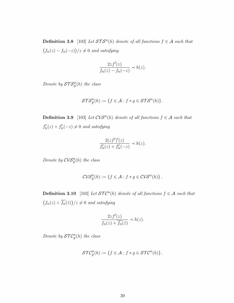
Definition 3.8 [103] Let ST Sn(h) denote of all functions f ∈ A such that(fn(z)− fn(−z)
)/z 6= 0 and satisfying
2zf ′(z)
fn(z)− fn(−z)≺ h(z).
Denote by ST Sng (h) the class
ST Sng (h) := f ∈ A : f ∗ g ∈ ST Sn(h) .
Definition 3.9 [103] Let CVSn(h) denote of all functions f ∈ A such that
f ′n(z) + f ′n(−z) 6= 0 and satisfying
2(zf ′)′(z)
f ′n(z) + f ′n(−z)≺ h(z).
Denote by CVSng (h) the class
CVSng (h) := f ∈ A : f ∗ g ∈ CVSn(h) .
Definition 3.10 [103] Let ST Cn(h) denote of all functions f ∈ A such that(fn(z) + fn(z)
)/z 6= 0 and satisfying
2zf ′(z)
fn(z) + fn(z)≺ h(z).
Denote by ST Cng (h) the class
ST Cng (h) := f ∈ A : f ∗ g ∈ ST Cn(h) .
39
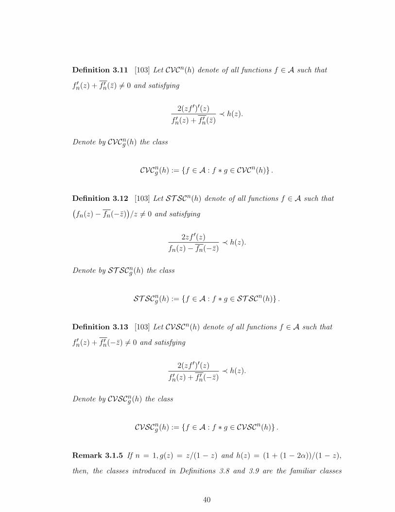
Definition 3.11 [103] Let CVCn(h) denote of all functions f ∈ A such that
f ′n(z) + f ′n(z) 6= 0 and satisfying
2(zf ′)′(z)
f ′n(z) + f ′n(z)≺ h(z).
Denote by CVCng (h) the class
CVCng (h) := f ∈ A : f ∗ g ∈ CVCn(h) .
Definition 3.12 [103] Let ST SCn(h) denote of all functions f ∈ A such that(fn(z)− fn(−z)
)/z 6= 0 and satisfying
2zf ′(z)
fn(z)− fn(−z)≺ h(z).
Denote by ST SCng (h) the class
ST SCng (h) := f ∈ A : f ∗ g ∈ ST SCn(h) .
Definition 3.13 [103] Let CVSCn(h) denote of all functions f ∈ A such that
f ′n(z) + f ′n(−z) 6= 0 and satisfying
2(zf ′)′(z)
f ′n(z) + f ′n(−z)≺ h(z).
Denote by CVSCng (h) the class
CVSCng (h) := f ∈ A : f ∗ g ∈ CVSCn(h) .
Remark 3.1.5 If n = 1, g(z) = z/(1 − z) and h(z) = (1 + (1 − 2α))/(1 − z),
then, the classes introduced in Definitions 3.8 and 3.9 are the familiar classes
40
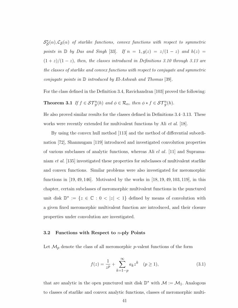
S∗S(α), CS(α) of starlike functions, convex functions with respect to symmetric
points in D by Das and Singh [33]. If n = 1, g(z) = z/(1 − z) and h(z) =
(1 + z)/(1 − z), then, the classes introduced in Definitions 3.10 through 3.13 are
the classes of starlike and convex functions with respect to conjugate and symmetric
conjugate points in D introduced by El-Ashwah and Thomas [39].
For the class defined in the Definition 3.4, Ravichandran [103] proved the following:
Theorem 3.1 If f ∈ ST ng (h) and φ ∈ Rα, then φ ∗ f ∈ ST ng (h).
He also proved similar results for the classes defined in Definitions 3.4–3.13. These
works were recently extended for multivalent functions by Ali et al. [18].
By using the convex hull method [113] and the method of differential subordi-
nation [72], Shanmugam [119] introduced and investigated convolution properties
of various subclasses of analytic functions, whereas Ali el al. [11] and Suprama-
niam et al. [135] investigated these properties for subclasses of multivalent starlike
and convex functions. Similar problems were also investigated for meromorphic
functions in [19, 49, 146]. Motivated by the works in [18, 19, 49, 103, 119], in this
chapter, certain subclasses of meromorphic multivalent functions in the punctured
unit disk D∗ := z ∈ C : 0 < |z| < 1 defined by means of convolution with
a given fixed meromorphic multivalent function are introduced, and their closure
properties under convolution are investigated.
3.2 Functions with Respect to n-ply Points
Let Mp denote the class of all meromorphic p-valent functions of the form
f(z) =1
zp+
∞∑k=1−p
akzk (p ≥ 1), (3.1)
that are analytic in the open punctured unit disk D∗ with M :=M1. Analogous
to classes of starlike and convex analytic functions, classes of meromorphic multi-
41
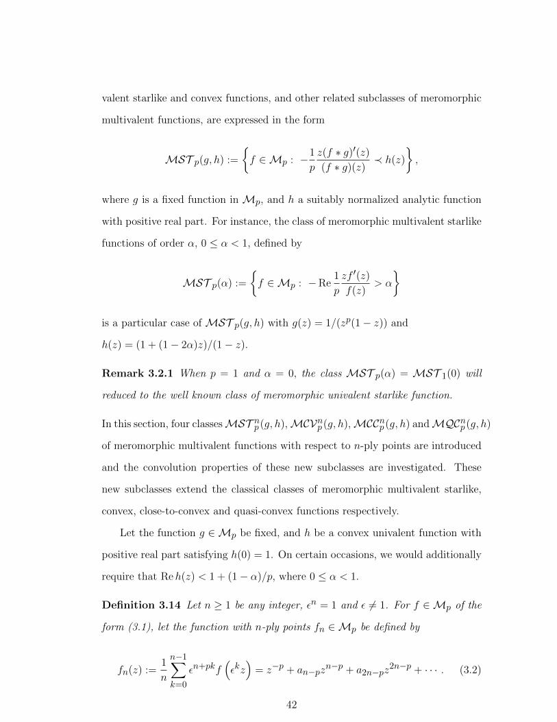
valent starlike and convex functions, and other related subclasses of meromorphic
multivalent functions, are expressed in the form
MST p(g, h) :=
f ∈Mp : −1
p
z(f ∗ g)′(z)
(f ∗ g)(z)≺ h(z)
,
where g is a fixed function in Mp, and h a suitably normalized analytic function
with positive real part. For instance, the class of meromorphic multivalent starlike
functions of order α, 0 ≤ α < 1, defined by
MST p(α) :=
f ∈Mp : −Re
1
p
zf ′(z)
f(z)> α
is a particular case of MST p(g, h) with g(z) = 1/(zp(1− z)) and
h(z) = (1 + (1− 2α)z)/(1− z).
Remark 3.2.1 When p = 1 and α = 0, the class MST p(α) = MST 1(0) will
reduced to the well known class of meromorphic univalent starlike function.
In this section, four classesMST np (g, h),MCVnp (g, h),MCCnp (g, h) andMQCnp (g, h)
of meromorphic multivalent functions with respect to n-ply points are introduced
and the convolution properties of these new subclasses are investigated. These
new subclasses extend the classical classes of meromorphic multivalent starlike,
convex, close-to-convex and quasi-convex functions respectively.
Let the function g ∈ Mp be fixed, and h be a convex univalent function with
positive real part satisfying h(0) = 1. On certain occasions, we would additionally
require that Reh(z) < 1 + (1− α)/p, where 0 ≤ α < 1.
Definition 3.14 Let n ≥ 1 be any integer, εn = 1 and ε 6= 1. For f ∈Mp of the
form (3.1), let the function with n-ply points fn ∈Mp be defined by
fn(z) :=1
n
n−1∑k=0
εn+pkf(εkz)
= z−p + an−pzn−p + a2n−pz2n−p + · · · . (3.2)
42

The classes of meromorphic multivalent starlike and convex functions with respect
to n-ply points are defined in the following definitions:
Definition 3.15 The class MST np (h) consists of functions f ∈ Mp satisfying
fn(z) 6= 0 in D∗ and the subordination
−1
p
zf ′(z)
fn(z)≺ h(z).
The general class MST np (g, h) consists of functions f ∈ Mp for which f ∗ g,
belongs to MST np (h).
Definition 3.16 The class MCVnp (h) consists of functions f ∈ Mp satisfying
f ′n(z) 6= 0 in D∗ and the subordination
−1
p
(zf ′(z)
)′f ′n(z)
≺ h(z).
The general classMCVnp (g, h) consists of functions f ∈Mp for which f∗g, belongs
to MCVnp (h).
Remark 3.2.2 If g(z) := 1/zp(1−z), then the classesMST np (g, h) andMCVnp (g, h)
coincide with MST np (h) and MCVnp (h) respectively. If p = 1 and n = 1, then
the classes MST np (g, h) and MCVnp (g, h) reduced respectively to MST (g, h) and
MCV(g, h) which were introduced and investigated in [49]. The notationMST p(h)
will be used for the class MST 1p(h).
Theorem 3.2 Let h be a convex univalent function satisfying
Reh(z) < 1 +1− αp
(0 ≤ α < 1), (3.3)
and φ ∈Mp with zp+1φ ∈ Rα.
(i) If f ∈MST np (g, h), then φ ∗ f ∈MST np (g, h).
43

(ii) If f ∈MCVnp (g, h), then φ ∗ f ∈MCVnp (g, h).
Proof. (i) The proof begins by showing that if f ∈MST np (h), then
φ ∗ f ∈MST np (h). Let f ∈MST np (h), and define the functions H and ψ by
H(z) := − zf′(z)
pfn(z)and ψ(z) := zp+1fn(z).
Thus for any fixed z ∈ D,
− zf′(z)
pfn(z)∈ h(D) (3.4)
Replacing z by εkz in (3.2), it follows that
fn(εkz) = (εkz)−p + an−p(εkz)n−p + a2n−p(εkz)2n−p + . . .
= ε−pkz−p + an−pεk(n−p)zn−p + a2n−pεk(2n−p)z2n−p + . . .
= ε−pkz−p + an−pεkn−kpzn−p + a2n−pε2kn−kpz2n−p + . . .
= ε−pkz−p + an−p(1)ε−pkzn−p + a2n−p(1)ε−kpz2n−p + . . . (εn = 1)
= ε−pk(z−p + an−pzn−p + a2n−pz
2n−p + . . .)
= ε−pkfn(z)
Therefore
fn(εkz) = ε−pkfn(z). (3.5)
By replacing z by εkz in (3.4), it follows that
−(εkz)f ′(εkz)
pfn(εkz)∈ h(D).
In view of (3.5), it is clear that
−(εkz)f ′(εkz)
pfn(εkz)= −(εkz)f ′(εkz)
pε−pkfn(z)
44

= −zεk+pkf ′(εkz)
pfn(z).
Thus, the containment (3.4) becomes
−zεk(1+p)f ′(εkz)
pfn(z)∈ h(D).
Since h(D) is a convex domain, this yields
− 1
n
n−1∑k=0
εk(1+p)zf ′(εkz)
pfn(z)∈ h(D). (3.6)
From (3.2), it is evident that
f ′n(z) =1
n
n−1∑k=0
ε(n+pk)f ′(εkz)εk
=1
n
n−1∑k=0
εk(1+p)f ′(εkz). (3.7)
Now, by using (3.7) in (3.6), it follows that
−zf′n(z)
pfn(z)∈ h(D)
and thus in terms of subordination becomes
−zf′n(z)
pfn(z)≺ h(z). (3.8)
Hence fn ∈MST p(h). Logarithmic differentiation of ψ(z) = zp+1fn(z) yields
zψ′(z)
ψ(z)=zf ′n(z)
fn(z)+ p+ 1. (3.9)
45

By applying (3.3) in (3.8), it follows that
−Re
(zf ′n(z)
pfn(z)
)< 1 +
1− αp
which in turn implies
Re
(zf ′n(z)
fn(z)
)> −p− 1 + α. (3.10)
From (3.9), it follows that
Re
(zψ′(z)
ψ(z)
)= Re
(zf ′n(z)
fn(z)
)+ p+ 1
and by using (3.3)
Re
(zψ′(z)
ψ(z)
)> −p− 1 + α + p+ 1 = α. (3.11)
Inequality (3.11) shows that the function ψ belongs to ST (α). Computation shows
that
− z(φ ∗ f)′(z)
p(φ ∗ f)n(z)=−zp−1(φ ∗ f)′(z)
(φ ∗ f)n(z)
=
(φ ∗ (−p−1zf ′)
)(z)
(φ ∗ fn)(z)
=
(φ ∗ (Hfn)
)(z)
(φ ∗ fn)(z)
=
(zp+1φ(z)
)∗(H(z)ψ(z)
)(zp+1φ(z)
)∗ (ψ(z))
.
Since zp+1φ ∈ Rα and ψ ∈ ST (α), Theorem 2.3 yields
(zp+1φ(z)
)∗(H(z)ψ(z)
)(zp+1φ(z)
)∗ (ψ(z))
∈ co(H(D)).
46

The subordination H ≺ h implies
− z(φ ∗ f)′(z)
p(φ ∗ f)n(z)≺ h(z).
Thus φ ∗ f ∈MST np (h). The general case follows from the fact that
f ∈MST np (g, h)⇔ f ∗ g ∈MST np (h). (3.12)
Indeed, if f ∈MST np (g, h), then f ∗ g ∈MST np (h), and therefore
φ ∗ f ∗ g ∈MST np (h), or equivalently φ ∗ f ∈MST np (g, h).
(ii) The identity
−(z(g ∗ f)′(z)
)′p(g ∗ f)′n(z)
= −z(g ∗ −p−1zf ′
)′(z)
p(g ∗ −p−1zf ′
)n(z)
shows that
f ∈MCVnp (g, h)⇔ −zf′
p∈MST np (g, h), (3.13)
and by the result of part (i), it is clear that
φ ∗(−zf
′
p
)∈MST np (g, h)
which implies
−z(φ ∗ f)′
p∈MST np (g, h).
Hence, in view of (3.13), φ ∗ f ∈MCVnp (g, h).
Corollary 3.2.1 The following inclusions hold:
(i) MST np (g, h) ⊂MST np (φ ∗ g, h)
(ii) MCVnp (g, h) ⊂MCVnp (φ ∗ g, h)
47

Proof. (i) In view of the fact (3.12) and Theorem 3.2(i), it is evident that φ∗f ∗g ∈
MST np (h), or equivalently f ∗ (φ ∗ g) ∈MST np (h). Hence f ∈MST np (φ ∗ g, h).
(ii) In view of the fact that f ∈ MCVnp (g, h) ⇔ f ∗ g ∈ MCVnp (h), and
Theorem 3.2(ii), it follows that φ ∗ f ∗ g ∈ MCVnp (h) or f ∗ (φ ∗ g) ∈ MCVnp (h).
Therefore f ∈MCVnp (φ ∗ g, h).
When n = 1 and p = 1, the following corollaries are easily deduced from Theorem
3.2(i) and Theorem 3.2(ii) respectively:
Corollary 3.2.2 [49, Theorem 3.3] Let h be a convex univalent function satisfying
Reh(z) < 2− α, 0 ≤ α < 1, and φ ∈ M with z2φ ∈ Rα. If f ∈ MST (g, h) then
φ ∗ f ∈MST (g, h).
Corollary 3.2.3 [49, Theorem 3.6] Let h be a convex univalent function satisfying
Reh(z) < 2 − α, 0 ≤ α < 1, and φ ∈ M with z2φ ∈ Rα. If f ∈ MCV(g, h) then
φ ∗ f ∈MCV(g, h).
If n = 1, p = 1 and g(z) = 1/z(1 − z), then the following result follows from
Theorem 3.2(i):
Corollary 3.2.4 [49, Theorem 3.5] Let h be a convex univalent function satisfying
Reh(z) < 2 − α, 0 ≤ α < 1, and φ ∈ M with z2φ ∈ Rα. If f ∈ MST (h), then
f ∈MST (φ, h)
The classes of meromorphic multivalent close-to-convex and quasi-convex functions
with respect to n-ply points are defined in the following definitions:
Definition 3.17 The class MCCnp (h) consists of functions f ∈Mp satisfying the
subordination
−1
p
zf ′(z)
φn(z)≺ h(z)
for some φ ∈ MST np (h) with φn(z) 6= 0 in D∗. The general class MCCnp (g, h)
consists of functions f ∈Mp for which f ∗ g, belongs to MCCnp (h).
48

Definition 3.18 The classMQCnp (h) consists of functions f ∈Mp satisfying the
subordination
−1
p
(zf ′(z)
)′ϕ′n(z)
≺ h(z)
for some ϕ ∈ MCVnp with ϕ′n(z) 6= 0 in D∗. The general class MQCnp (g, h)
consists of functions f ∈Mp for which f ∗ g, belongs to MQCnp (h).
Remark 3.2.3 If g(z) := 1/zp(1−z), then the classesMCCnp (g, h) andMQCnp (g, h)
coincide with MCCnp (h) and MQCnp (h) respectively. If p = 1 and n = 1, then
the classes MCCnp (g, h) and MQCnp (g, h) reduced respectively to MCC(g, h) and
MQC(g, h) which were introduced and investigated in [49].
Theorem 3.3 Let h be a convex univalent function satisfying
Reh(z) < 1 +1− αp
(0 ≤ α < 1),
and φ ∈Mp with zp+1φ ∈ Rα.
(i) If f ∈MCCnp (g, h) with respect to a function ϕ ∈MST np (g, h),
then φ ∗ f ∈MCCnp (g, h) with respect to φ ∗ ϕ ∈MST np (g, h).
(ii) If f ∈MQCnp (g, h) with respect to a function ϕ ∈MCVnp (g, h),
then φ ∗ f ∈MQCnp (g, h) with respect to φ ∗ ϕ ∈MCVnp (g, h).
Proof. (i) It is sufficient to prove that φ ∗ f ∈MCCnp (h) whenever f ∈MCCnp (h).
Let f ∈MCCnp (h) with respect to a function ϕ ∈MST np (h). Since
ϕ ∈MST np (h),
Theorem 3.2 yields
φ ∗ ϕ ∈MST np (h).
49

Also it is easy to see from (3.8) and (3.3) that
ϕn ∈MST p(h) and zp+1ϕn(z) ∈ ST (α).
Now, define the functions H(z) and ψ(z) by
H(z) = − zf′(z)
pϕn(z)and ψ(z) = zp+1ϕn(z).
Since zp+1φ(z) ∈ Rα and H(z) ≺ h(z), an application of Theorem 2.3 shows that
− z(φ ∗ f)′(z)
p(φ ∗ ϕ)n(z)
=
(φ ∗ (−zp−1f ′)
)(z)
(φ ∗ ϕn)(z)
=
(φ ∗ (H(z)ϕn)
)(z)
(φ ∗ ϕn)(z)
=
(zp+1φ(z)
)∗ (H(z)ψ(z))(
zp+1φ(z))∗ (ψ(z))
≺ h(z).
Thus φ ∗ f ∈MCCnp (h). The general case follows from the fact that
f ∈MCCnp (g, h)⇔ f ∗ g ∈MCCnp (h). (3.14)
Indeed, if f ∈MCCnp (g, h), then f ∗ g ∈MCCnp (h), and therefore
φ ∗ f ∗ g ∈MCCnp (h), or equivalently φ ∗ f ∈MCCnp (g, h).
(ii) The proof begins with the identity
−(z(g ∗ f)′(z)
)′p(g ∗ ϕ)′n(z)
= −z(g ∗ −zf
′p
)′(g ∗ −zϕ
′p
)n
,
50

which shows that the function
f ∈MQCnp (g, h)⇔ −zf′
p∈MCCnp (g, h). (3.15)
From the result of part (i), it follows that
φ ∗(−zf
′
p
)∈MCCnp (g, h)
which implies
−zp
(φ ∗ f)′(z) ∈MCCnp (g, h).
Hence, in view of (3.15) φ ∗ f ∈MQCnp (g, h). This complete the proof.
Corollary 3.2.5 The following inclusions hold:
(i) MCCnp (g, h) ⊂MCCnp (φ ∗ g, h)
(ii) MQCnp (g, h) ⊂MQCnp (φ ∗ g, h)
Proof. (i) From the fact (3.14), it is clear that if f ∈ MCCnp (g, h), then f ∗ g ∈
MCCnp (h). Theorem 3.3(i), yields φ ∗ f ∗ g ∈MCCnp (h), or f ∗ (φ ∗ g) ∈MCCnp (h).
Therefore f ∈MCCnp (φ ∗ g, h).
(ii) From the fact that f ∈ MQCnp (g, h) ⇔ f ∗ g ∈ MQCnp (h), and Theo-
rem 3.3(ii), it follows that φ ∗ f ∗ g ∈MQCnp (h) or f ∗ (φ ∗ g) ∈MQCnp (h) Hence
f ∈MQCnp (φ ∗ g, h). This complete the proof.
When n = 1 and p = 1, the following corollaries are special cases of Theorem 3.3(i)
and Theorem 3.3(ii) respectively:
Corollary 3.2.6 [49, Theorem 3.7] Under the conditions of Corollary 3.2.2, if
f ∈ MCC(g, h) with respect to ψ ∈ MST (g, h), then φ ∗ f ∈ MCC(g, h) with
respect to φ ∗ ψ ∈MST (g, h).
51

Corollary 3.2.7 [49, Theorem 3.12] Let h and φ satisfy the conditions of Corol-
lary 3.2.2. If f ∈MQC(g, h), then φ ∗ f ∈MQC(g, h).
3.3 Functions with Respect to n-ply Symmetric Points
In this section and the following two sections, it is assumed that p is an odd
number. As before, it is assumed that the function g ∈Mp is a fixed function and
the function h is convex univalent with positive real part satisfying h(0) = 1.
The classes of meromorphic multivalent starlike and convex functions with
respect to n-ply symmetric points are defined in the following definitions:
Definition 3.19 For odd integer p, the class MST Snp (h) consists of functions
f ∈Mp satisfying fn(z)− fn(−z) 6= 0 in D∗ and the subordination
−1
p
2zf ′(z)
fn(z)− fn(−z)≺ h(z). (3.16)
The general class MST Snp (g, h) consists of functions f ∈ Mp for which f ∗ g,
belongs to MST Snp (h).
Definition 3.20 For odd integer p, the class MCVSnp (h) consists of functions
f ∈Mp satisfying f ′n(z) + f ′n(−z) 6= 0 in D∗ and the subordination
−1
p
2(zf ′)′
(z)
f ′n(z) + f ′n(−z)≺ h(z).
The general class MCVSnp (g, h) consists of functions f ∈ Mp for which f ∗ g,
belongs to MCVSnp (h).
Theorem 3.4 Let h be a convex univalent function satisfying
Reh(z) < 1 +1− αp
(0 ≤ α < 1),
52

and φ ∈Mp with zp+1φ ∈ Rα.
(i) If f ∈MST Snp (g, h), then φ ∗ f ∈MST Snp (g, h).
(ii) If f ∈MCVSnp (g, h), then φ ∗ f ∈MCVSnp (g, h).
Proof. (i) It is enough to show that if f is inMST Snp (h), then so is φ ∗ f . Define
the functions Fn, H and Ψ by
Fn(z) =fn(z)− fn(−z)
2, H(z) := − zf
′(z)
pFn(z)and Ψ(z) := zp+1Fn(z).
When n = 1, F(1)(z) = F (z).
Let f ∈MST Snp (h). Thus for any fixed z ∈ D,
− zf′(z)
pFn(z)∈ h(D). (3.17)
Replacing z by −z in (3.17) and taking the convex combinations, it follows that
− zf ′(z)
2pFn(z)− (−z)f ′(−z)
2pFn(−z)= − 1
2p
(zf ′(z)
Fn(z)+
(−z)f ′(−z)
Fn(−z)
)= − 1
2p
(zf ′(z)
Fn(z)+
(−z)f ′(−z)
−Fn(z)
)
= −z(f ′(z)+f ′(−z)
2
)pFn(z)
∈ h(D)
which implies
− zF′(z)
pFn(z)∈ h(D).
This shows that the function F ∈ MST np (h), and the proof of Theorem 3.2 now
shows that Fn ∈MST p(h), or
−zF′n(z)
pFn(z)≺ h(z). (3.18)
53

A computation from
Ψ(z) = zp+1Fn(z)
shows that
zΨ′(z)
Ψ(z)=zF ′n(z)
Fn(z)+ p+ 1. (3.19)
By applying (3.3) in (3.18), it follows that
−Re
(zF ′n(z)
pFn(z)
)< 1 +
1− αp
which implies
Re
(zF ′n(z)
Fn(z)
)> −p− 1 + α. (3.20)
From (3.19), it is clear that
Re
(zΨ′(z)
Ψ(z)
)= Re
(zF ′n(z)
Fn(z)
)+ p+ 1
and by using (3.20)
Re
(zΨ′(z)
Ψ(z)
)> −p− 1 + α + p+ 1 = α. (3.21)
Inequality (3.21) shows that the function Ψ belongs to ST (α). Another computa-
tion shows that
−2
p
z(φ ∗ f)′(z)
(φ ∗ f)n(z)− (φ ∗ f)n(−z)=
φ(z) ∗ −zp−1f ′(z)
φ(z) ∗ fn(z)−fn(−z)2
=(φ ∗HFn)(z)
(φ ∗ Fn)(z).
Since zp+1φ ∈ Rα and Ψ ∈ ST (α), Theorem 2.3 yields
(φ ∗HFn)(z)
(φ ∗ Fn)(z)=
(zp+1φ(z)
)∗(H(z)ψ(z)
)(zp+1φ(z)
)∗(ψ(z)
) ∈ co(H(D)
),
54

and because H(z) ≺ h(z), it follows that
−2
p
z(φ ∗ f)′(z)
(φ ∗ f)n(z)− (φ ∗ f)n(−z)=
(φ ∗HFn)(z)
(φ ∗ Fn)(z)≺ h(z).
Hence φ ∗ f ∈MST Snp (h).The general result is obtained from the fact that
f ∈MST Snp (g, h)⇔ f ∗ g ∈MST Snp (h)
which gives φ ∗ f ∗ g ∈MST Snp (h) or equivalently φ ∗ f ∈MST Snp (g, h).
(ii) The identity
− 2(z(g ∗ f)′(z))′
p((g ∗ f)′n(z) + (g ∗ f)′n(−z)
) = −2z(g ∗ −zf
′p
)′(z)
p((g ∗ −zf
′p
)n
(z)−(g ∗ −zf
′p
)n
(−z))
shows that
f ∈MCVSnp (g, h)⇔ −zf′
p∈MST Snp (g, h), (3.22)
and, by the result of part (i), it is clear that
φ ∗(−zf
′
p
)∈MST Snp (g, h)
which implies
−z(φ ∗ f)′
p∈MST Snp (g, h).
Hence, in view of (3.22), φ ∗ f ∈MCVSnp (g, h).
3.4 Functions with Respect to n-ply Conjugate Points
The classes of meromorphic multivalent starlike and convex functions with respect
to n-ply conjugate points are defined in the following definitions:
Definition 3.21 For odd integer p, the class MST Cnp (h) consists of functions
55
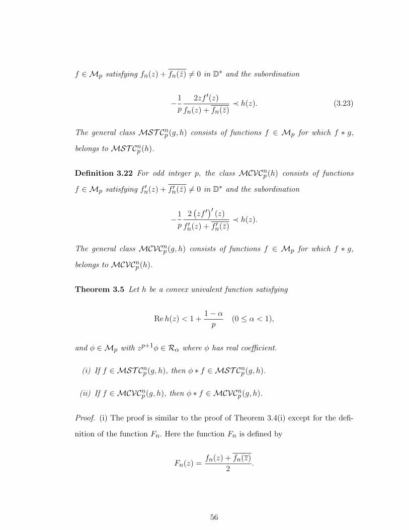
f ∈Mp satisfying fn(z) + fn(z) 6= 0 in D∗ and the subordination
−1
p
2zf ′(z)
fn(z) + fn(z)≺ h(z). (3.23)
The general class MST Cnp (g, h) consists of functions f ∈ Mp for which f ∗ g,
belongs to MST Cnp (h).
Definition 3.22 For odd integer p, the class MCVCnp (h) consists of functions
f ∈Mp satisfying f ′n(z) + f ′n(z) 6= 0 in D∗ and the subordination
−1
p
2(zf ′)′
(z)
f ′n(z) + f ′n(z)≺ h(z).
The general class MCVCnp (g, h) consists of functions f ∈ Mp for which f ∗ g,
belongs to MCVCnp (h).
Theorem 3.5 Let h be a convex univalent function satisfying
Reh(z) < 1 +1− αp
(0 ≤ α < 1),
and φ ∈Mp with zp+1φ ∈ Rα where φ has real coefficient.
(i) If f ∈MST Cnp (g, h), then φ ∗ f ∈MST Cnp (g, h).
(ii) If f ∈MCVCnp (g, h), then φ ∗ f ∈MCVCnp (g, h).
Proof. (i) The proof is similar to the proof of Theorem 3.4(i) except for the defi-
nition of the function Fn. Here the function Fn is defined by
Fn(z) =fn(z) + fn(z)
2.
56
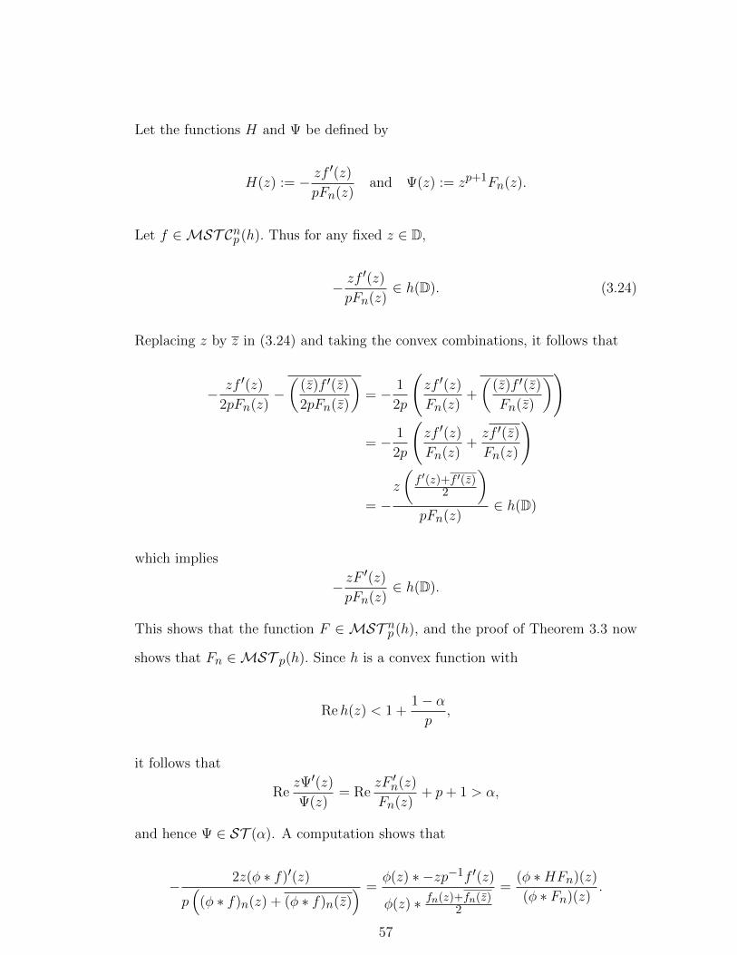
Let the functions H and Ψ be defined by
H(z) := − zf′(z)
pFn(z)and Ψ(z) := zp+1Fn(z).
Let f ∈MST Cnp (h). Thus for any fixed z ∈ D,
− zf′(z)
pFn(z)∈ h(D). (3.24)
Replacing z by z in (3.24) and taking the convex combinations, it follows that
− zf ′(z)
2pFn(z)−(
(z)f ′(z)
2pFn(z)
)= − 1
2p
(zf ′(z)
Fn(z)+
((z)f ′(z)
Fn(z)
))
= − 1
2p
(zf ′(z)
Fn(z)+zf ′(z)
Fn(z)
)
= −z
(f ′(z)+f ′(z)
2
)pFn(z)
∈ h(D)
which implies
− zF′(z)
pFn(z)∈ h(D).
This shows that the function F ∈ MST np (h), and the proof of Theorem 3.3 now
shows that Fn ∈MST p(h). Since h is a convex function with
Reh(z) < 1 +1− αp
,
it follows that
RezΨ′(z)
Ψ(z)= Re
zF ′n(z)
Fn(z)+ p+ 1 > α,
and hence Ψ ∈ ST (α). A computation shows that
− 2z(φ ∗ f)′(z)
p(
(φ ∗ f)n(z) + (φ ∗ f)n(z)) =
φ(z) ∗ −zp−1f ′(z)
φ(z) ∗ fn(z)+fn(z)2
=(φ ∗HFn)(z)
(φ ∗ Fn)(z).
57
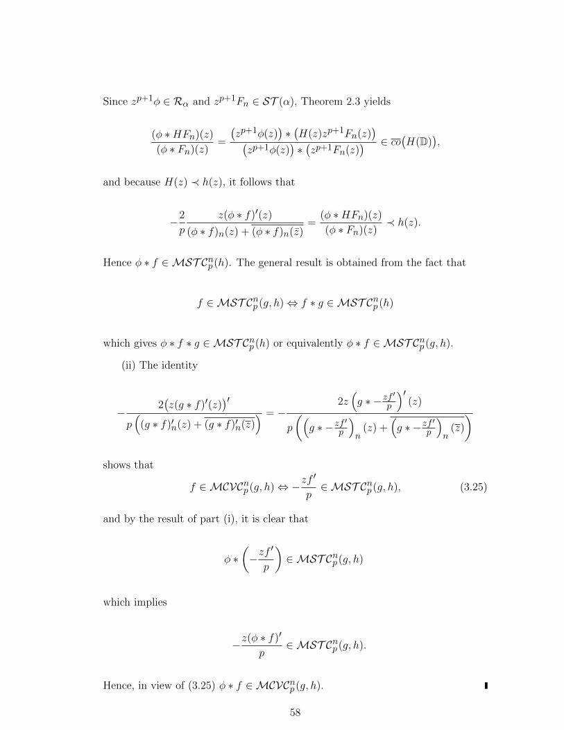
Since zp+1φ ∈ Rα and zp+1Fn ∈ ST (α), Theorem 2.3 yields
(φ ∗HFn)(z)
(φ ∗ Fn)(z)=
(zp+1φ(z)
)∗(H(z)zp+1Fn(z)
)(zp+1φ(z)
)∗(zp+1Fn(z)
) ∈ co(H(D)
),
and because H(z) ≺ h(z), it follows that
−2
p
z(φ ∗ f)′(z)
(φ ∗ f)n(z) + (φ ∗ f)n(z)=
(φ ∗HFn)(z)
(φ ∗ Fn)(z)≺ h(z).
Hence φ ∗ f ∈MST Cnp (h). The general result is obtained from the fact that
f ∈MST Cnp (g, h)⇔ f ∗ g ∈MST Cnp (h)
which gives φ ∗ f ∗ g ∈MST Cnp (h) or equivalently φ ∗ f ∈MST Cnp (g, h).
(ii) The identity
−2(z(g ∗ f)′(z)
)′p(
(g ∗ f)′n(z) + (g ∗ f)′n(z)) = −
2z(g ∗ −zf
′p
)′(z)
p
((g ∗ −zf
′p
)n
(z) +(g ∗ −zf
′p
)n
(z)
)
shows that
f ∈MCVCnp (g, h)⇔ −zf′
p∈MST Cnp (g, h), (3.25)
and by the result of part (i), it is clear that
φ ∗(−zf
′
p
)∈MST Cnp (g, h)
which implies
−z(φ ∗ f)′
p∈MST Cnp (g, h).
Hence, in view of (3.25) φ ∗ f ∈MCVCnp (g, h).
58

3.5 Functions with Respect to n-ply Symmetric Conjugate Points
The classes of meromorphic multivalent starlike and convex functions with respect
to n-ply symmetric conjugate points are defined in the following definitions:
Definition 3.23 For odd integer p, the class MST SCnp (h) consists of functions
f ∈Mp satisfying fn(z)− fn(−z) 6= 0 in D∗ and the subordination
−1
p
2zf ′(z)
fn(z)− fn(−z)≺ h(z). (3.26)
The general class MST SCnp (g, h) consists of functions f ∈ Mp for which f ∗ g,
belongs to MST SCnp (h).
Definition 3.24 For odd integer p, the class MCVSCnp (h) consists of functions
f ∈Mp satisfying f ′n(z) + f ′n(−z) 6= 0 in D∗ and the subordination
−1
p
2(zf ′)′
(z)
f ′n(z) + f ′n(−z)≺ h(z).
The general class MCVSCnp (g, h) consists of functions f ∈ Mp for which f ∗ g,
belongs to MCVSCnp (h).
Theorem 3.6 Let h be a convex univalent function satisfying
Reh(z) < 1 +1− αp
(0 ≤ α < 1),
and φ ∈Mp with zp+1φ ∈ Rα where φ has real coefficient.
(i) If f ∈MST SCnp (g, h), then φ ∗ f ∈MST SCnp (g, h).
(ii) If f ∈MCVSCnp (g, h), then φ ∗ f ∈MCVSCnp (g, h).
59
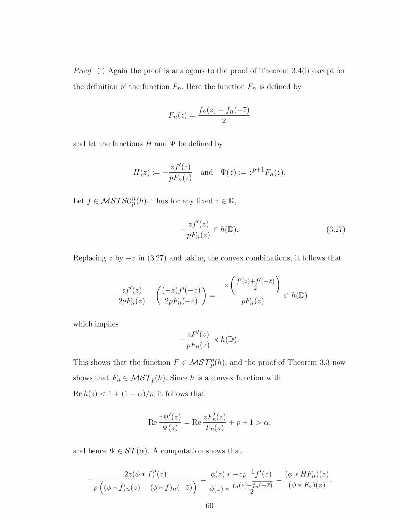
Proof. (i) Again the proof is analogous to the proof of Theorem 3.4(i) except for
the definition of the function Fn. Here the function Fn is defined by
Fn(z) =fn(z)− fn(−z)
2
and let the functions H and Ψ be defined by
H(z) := − zf′(z)
pFn(z)and Ψ(z) := zp+1Fn(z).
Let f ∈MST SCnp (h). Thus for any fixed z ∈ D,
− zf′(z)
pFn(z)∈ h(D). (3.27)
Replacing z by −z in (3.27) and taking the convex combinations, it follows that
− zf ′(z)
2pFn(z)−(
(−z)f ′(−z)
2pFn(−z)
)= −
z
(f ′(z)+f ′(−z)
2
)pFn(z)
∈ h(D)
which implies
− zF′(z)
pFn(z)≺ h(D).
This shows that the function F ∈ MST np (h), and the proof of Theorem 3.3 now
shows that Fn ∈MST p(h). Since h is a convex function with
Reh(z) < 1 + (1− α)/p, it follows that
RezΨ′(z)
Ψ(z)= Re
zF ′n(z)
Fn(z)+ p+ 1 > α,
and hence Ψ ∈ ST (α). A computation shows that
− 2z(φ ∗ f)′(z)
p(
(φ ∗ f)n(z)− (φ ∗ f)n(−z)) =
φ(z) ∗ −zp−1f ′(z)
φ(z) ∗ fn(z)−fn(−z)2
=(φ ∗HFn)(z)
(φ ∗ Fn)(z).
60

Since zp+1φ ∈ Rα and zp+1Fn ∈ ST (α), Theorem 2.3 yields
(φ ∗HFn)(z)
(φ ∗ Fn)(z)=
(zp+1φ(z)
)∗(H(z)zp+1Fn(z)
)(zp+1φ(z)
)∗(zp+1Fn(z)
) ∈ co(H(D)
),
and because H(z) ≺ h(z), it follows that
−2
p
z(φ ∗ f)′(z)
(φ ∗ f)n(z)− (φ ∗ f)n(−z)=
(φ ∗HFn)(z)
(φ ∗ Fn)(z)≺ h(z).
Hence φ ∗ f ∈MST SCnp (h). The general result is obtained from the fact that
f ∈MST SCnp (g, h)⇔ f ∗ g ∈MST SCnp (h)
which gives φ ∗ f ∗ g ∈MST SCnp (h) or equivalently φ ∗ f ∈MST SCnp (g, h).
(ii) The identity
− 2(z(g ∗ f)′(z))′
p(
(g ∗ f)′n(z) + (g ∗ f)′n(−z)) = −
2z(g ∗ −zf
′p
)′(z)
p
((g ∗ −zf
′p
)n
(z)−(g ∗ −zf
′p
)n
(−z)
)
shows that
f ∈MCVSCnp (g, h)⇔ −zf′
p∈MST SCnp (g, h), (3.28)
and by the result of part (i), it is clear that
φ ∗(−zf
′
p
)∈MST SCnp (g, h)
which implies
−z(φ ∗ f)′
p∈MST SCnp (g, h).
Hence, in view of (3.28) φ ∗ f ∈MCVSCnp (g, h).
61
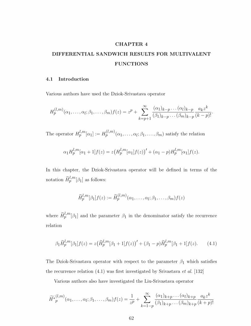
CHAPTER 4
DIFFERENTIAL SANDWICH RESULTS FOR MULTIVALENT
FUNCTIONS
4.1 Introduction
Various authors have used the Dziok-Srivastava operator
H(l,m)p (α1, . . . , αl; β1, . . . , βm)f(z) = zp +
∞∑k=p+1
(α1)k−p . . . (αl)k−p(β1)k−p . . . (βm)k−p
akzk
(k − p)!.
The operator Hl,mp [α1] := H
(l,m)p (α1, . . . , αl; β1, . . . , βm) satisfy the relation
α1Hl,mp [α1 + 1]f(z) = z
(Hl,mp [α1]f(z)
)′+ (α1 − p)H
l,mp [α1]f(z).
In this chapter, the Dziok-Srivastava operator will be defined in terms of the
notation Hl,mp [β1] as follows:
Hl,mp [β1]f(z) := H
(l,m)p (α1, . . . , αl; β1, . . . , βm)f(z)
where Hl,mp [β1] and the parameter β1 in the denominator satisfy the recurrence
relation
β1Hl,mp [β1]f(z) = z
(Hl,mp [β1 + 1]f(z)
)′+ (β1 − p)H
l,mp [β1 + 1]f(z). (4.1)
The Dziok-Srivastava operator with respect to the parameter β1 which satisfies
the recurrence relation (4.1) was first investigated by Srivastava et al. [132]
Various authors also have investigated the Liu-Srivastava operator
H∗(l,m)p (α1, . . . , αl; β1, . . . , βm)f(z) =
1
zp+
∞∑k=1−p
(α1)k+p . . . (αl)k+p
(β1)k+p . . . (βm)k+p
akzk
(k + p)!
62

where is framed using the notation Hl,mp [α1]f(z). Their works exploited the recur-
rence relation involving the parameter α1 in the numerator satisfying
α1Hl,mp [α1 + 1]f(z) = z
(Hl,mp [α1]f(z)
)′+ (α1 + p)H
l,mp [α1]f(z).
In this chapter, the parameter β1 in the denominator of Liu-Srivastava operator
which also satisfies a recurrence relation will be investigated. Denoting the Liu-
Srivastava operator by H∗l,mp [β1]f(z), it can be shown that
β1H∗l,mp [β1]f(z) = z
(H∗
l,mp [β1 + 1]f(z)
)′+ (β1 + p)H∗
l,mp [β1 + 1]f(z). (4.2)
4.2 Subordination of the Dziok-Srivastava Operator
In this section, the differential subordination result of Miller and Mocanu in The-
orem 2.1 is extended for functions associated with the Dziok-Srivastava linear
operator Hl,mp [β1]. A similar problem was studied by Aghalary et al. [1]. Related
results may also found in the works of [12–15, 23, 24, 58]. The following class of
admissible functions will be required to obtain the main results.
Definition 4.1 Let Ω be a set in C and q ∈ Q0 ∩H[0, p]. The class of admissible
functions ΦH [Ω, q] consists of those functions φ : C3 × D → C that satisfy the
admissibility condition φ(u, v, w; z) 6∈ Ω whenever
u = q(ζ), v =kζq′(ζ) + (β1 + 1− p)q(ζ)
β1 + 1(β1 ∈ C \ 0,−1,−2, . . .),
Re
(β1(β1 + 1)w + (p− β1)(β1 − p+ 1)u
(β1 + 1)v + (p− β1 − 1)u− (2(β1 − p) + 1)
)≥ kRe
(ζq′′(ζ)
q′(ζ)+ 1
),
z ∈ D, ζ ∈ ∂D \ E(q) and k ≥ p.
In the particular case q(z) = Mz, M > 0, and in view of Definition 4.1, the
following definition is immediate.
63
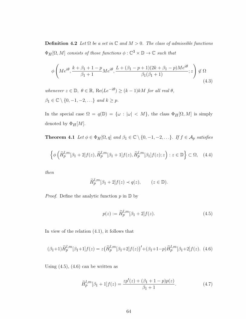
Definition 4.2 Let Ω be a set in C and M > 0. The class of admissible functions
ΦH [Ω,M ] consists of those functions φ : C3 × D→ C such that
φ
(Meiθ,
k + β1 + 1− pβ1 + 1
Meiθ,L+ (β1 − p+ 1)(2k + β1 − p)Meiθ
β1(β1 + 1); z
)6∈ Ω
(4.3)
whenever z ∈ D, θ ∈ R, Re(Le−iθ) ≥ (k − 1)kM for all real θ,
β1 ∈ C \ 0,−1,−2, . . . and k ≥ p.
In the special case Ω = q(D) = ω : |ω| < M, the class ΦH [Ω,M ] is simply
denoted by ΦH [M ].
Theorem 4.1 Let φ ∈ ΦH [Ω, q] and β1 ∈ C \ 0,−1,−2, . . .. If f ∈ Ap satisfies
φ(Hl,mp [β1 + 2]f(z), H
l,mp [β1 + 1]f(z), H
l,mp [β1]f(z); z
): z ∈ D
⊂ Ω, (4.4)
then
Hl,mp [β1 + 2]f(z) ≺ q(z), (z ∈ D).
Proof. Define the analytic function p in D by
p(z) := Hl,mp [β1 + 2]f(z). (4.5)
In view of the relation (4.1), it follows that
(β1+1)Hl,mp [β1+1]f(z) = z
(Hl,mp [β1+2]f(z)
)′+(β1+1−p)H l,m
p [β1+2]f(z). (4.6)
Using (4.5), (4.6) can be written as
Hl,mp [β1 + 1]f(z) =
zp′(z) + (β1 + 1− p)p(z)
β1 + 1. (4.7)
64

From (4.1), further computations show that
Hl,mp [β1]f(z) =
z2p′′(z) + 2(β1 − p+ 1)zp′(z) + (β1 − p)(β1 − p+ 1)p(z)
β1(β1 + 1). (4.8)
Define the transformation ψ from C3 to C by
u = r, v =s+ (β1 + 1− p)r
β1 + 1, w =
t+ 2(β1 − p+ 1)s+ (β1 − p)(β1 − p+ 1)r
β1(β1 + 1),
(4.9)
where
r = p(z), s = zp′(z) and t = z2p′′(z).
Let
ψ(r, s, t; z) = φ(u, v, w; z)
= φ
(r,s+ (β1 + 1− p)r
β1 + 1,t+ 2(β1 − p+ 1)s+ (β1 − p)(β1 − p+ 1)r
β1(β1 + 1); z
).
(4.10)
From (4.5), (4.7) and (4.8), the equation (4.10), yields
ψ(p(z), zp′(z), z2p′′(z); z
)= φ
(Hl,mp [β1 + 2]f(z), H
l,mp [β1 + 1]f(z), H
l,mp [β1]f(z); z
).
(4.11)
Hence (4.4) becomes
ψ(p(z), zp′(z), z2p′′(z); z
)∈ Ω.
To complete the proof, it is left to show that the admissibility condition for
φ ∈ ΦH [Ω, q] is equivalent to the admissibility condition for ψ as given in Definition
2.1. Note that
v =s+ (β1 + 1− p)r
β1 + 1
65

implies
s = v(β1 + 1)− (β1 + 1− p)r.
Computation from
w =t+ 2(β1 − p+ 1)s+ (β1 − p)(β1 − p+ 1)r
β1(β1 + 1)
shows that
t
s+ 1 =
wβ1(β1 + 1)− (β1 − p)(β1 − p+ 1)u
v(β1 + 1)− (β1 + 1− p)u−(2(β1 − p) + 1
)(u = r).
Hence ψ ∈ Ψp[Ω, q]. By Theorem 2.1, p(z) ≺ q(z) or
Hl,mp [β1 + 2]f(z) ≺ q(z).
If Ω 6= C is a simply connected domain, then Ω = h(D) for some conformal
mapping h of D onto Ω. In this case the class ΦH [h(D), q] is written as ΦH [h, q].
The following result is an immediate consequence of Theorem 4.1.
Theorem 4.2 Let φ ∈ ΦH [h, q] and β1 ∈ C \ 0,−1,−2, . . .. If f ∈ Ap satisfies
φ(Hl,mp [β1 + 2]f(z), H
l,mp [β1 + 1]f(z), H
l,mp [β1]f(z); z
)≺ h(z), (4.12)
then
Hl,mp [β1 + 2]f(z) ≺ q(z).
The next result is an extension of Theorem 4.1 to the case where the behavior of
q on ∂D is not known.
Corollary 4.2.1 Let Ω ⊂ C, q be univalent in D and q(0) = 0. Let φ ∈ ΦH [Ω, qρ]
for some ρ ∈ (0, 1) where qρ(z) = q(ρz) and β1 ∈ C \ 0,−1,−2, . . .. If f ∈ Ap66

and
φ(Hl,mp [β1 + 2]f(z), H
l,mp [β1 + 1]f(z), H
l,mp [β1]f(z); z
)∈ Ω,
then
Hl,mp [β1 + 2]f(z) ≺ q(z).
Proof. Theorem 4.1 yields Hl,mp [β1+2]f(z) ≺ qρ(z). The result follows easily from
the subordination qρ(z) ≺ q(z).
Theorem 4.3 Let h and q be univalent in D, with q(0) = 0, set qρ(z) = q(ρz)
and hρ(z) = h(ρz) and β1 ∈ C \ 0,−1,−2, . . .. Let φ : C3 × D → C satisfy one
of the following conditions:
1. φ ∈ ΦH [h, qρ] for some ρ ∈ (0, 1), or
2. there exists ρ0 ∈ (0, 1) such that φ ∈ ΦH [hρ, qρ] for all ρ ∈ (ρ0, 1).
If f ∈ Ap satisfies (4.12), then
Hl,mp [β1 + 2]f(z) ≺ q(z).
Proof. (1) The function qρ is univalent on D, and therefore E(qρ) is empty and
qρ ∈ Q. The class ΦH [h, qρ] is an admissible class and from Theorem 4.1 we obtain
Hl,mp [β1 + 2]f(z) ≺ qρ(z).
Since qρ ≺ q we deduce Hl,mp [β1 + 2]f(z) ≺ q(z).
(2) From (4.11), it is evident that
φ ∈ ΦH [hρ, qρ]
implies
ψ ∈ ΨH [hp, qp].
67

If we let pρ(z) = p(ρz), then
ψ(pρ(z), zp′ρ(z), z2p′′ρ(z); ρz
)= ψ
(p(ρz), ρzp′(ρz), ρ2z2p′′(ρz); ρz
)∈ hρ(D).
By using Thorem 2.1, with ρz, a function mapping D into D we obtain
pρ(z) ≺ qρ(z), for ρ ∈ (ρ0, 1). By letting ρ → 1− we obtain p(z) ≺ q(z) or
Hl,mp [β1 + 2]f(z) ≺ q(z).
The next theorem yields the best dominant of the differential subordination (4.12).
Theorem 4.4 Let h be univalent in D, φ : C3×D→ C and β1 ∈ C\0,−1,−2, . . ..
Suppose that the differential equation
φ(q(z), zq′(z), z2q′′(z); z
)= h(z) (4.13)
has a solution q with q(0) = 0 and satisfy one of the following conditions:
1. q ∈ Q0 and φ ∈ ΦH [h, q],
2. q is univalent in D and φ ∈ ΦH [h, qρ] for some ρ ∈ (0, 1), or
3. q is univalent in D and there exists ρ0 ∈ (0, 1) such that φ ∈ ΦH [hρ, qρ] for
all ρ ∈ (ρ0, 1).
If f ∈ Ap satisfies (4.12), then
Hl,mp [β1 + 2]f(z) ≺ q(z),
and q(z) is the best dominant.
Proof. In view of Theorem 4.2 and Theorem 4.3 we deduce that q is a dominant
of (4.12) . Since q satisfies (4.13), it is also a solution of (4.12) and therefore q will
be dominated by all dominants. Hence q is the best dominant.
68

Corollary 4.2.2 Let φ ∈ ΦH [Ω,M ] and β1 ∈ C \ 0,−1,−2, . . .. If f ∈ Ap
satisfies
φ(Hl,mp [β1 + 2]f(z), H
l,mp [β1 + 1]f(z), H
l,mp [β1]f(z); z
)∈ Ω,
then ∣∣∣H l,mp [β1 + 2]f(z)
∣∣∣ < M.
Proof. The result follows by taking q(z) = Mz in Theorem 4.1.
Corollary 4.2.3 Let φ ∈ ΦH [M ] and β1 ∈ C\0,−1,−2, . . .. If f ∈ Ap satisfies
∣∣∣φ(H l,mp [β1 + 2]f(z), H
l,mp [β1 + 1]f(z), H
l,mp [β1]f(z); z
)∣∣∣ < M,
then ∣∣∣H l,mp [β1 + 2]f(z)
∣∣∣ < M.
Proof. By taking Ω = q(D) in Corollary 4.2.2, the result is obtained.
Taking φ(u, v, w; z) = v in Corollary 4.2.3 leads to the following example.
Example 4.1 If Re β1 ≥ (p− 3)/2 and f ∈ Ap satisfies
∣∣∣H l,mp [β1 + 1]f(z)
∣∣∣ < M,
then ∣∣∣H l,mp [β1 + 2]f(z)
∣∣∣ < M.
Proof. By taking φ(u, v, w; z) = v in Corollary 4.2.3, we have to find the condition
so that φ ∈ ΦH [M ], that is, the admissibility condition (4.3) is satisfied. This
follows from
∣∣∣∣∣φ(Meiθ,
k + β1 + 1− pβ1 + 1
Meiθ,L+ (β1 − p+ 1)(2k + β1 − p)Meiθ
β1(β1 + 1); z
)∣∣∣∣∣ ≥M
69

which implies
∣∣∣∣k + β1 + 1− pβ1 + 1
Meiθ∣∣∣∣ ≥M
or
|k + β1 + 1− p| ≥ |β1 + 1|. (4.14)
Preceding inequality (4.14), shows that
Re β1 ≥p− k
2− 1.
Since k ≥ 1, then it is sufficient to write
Re β1 ≥p− 3
2
for (4.14) holds true.
Hence, from Corollary 4.2.3, if Re β1 ≥ (p− 3)/2 and∣∣∣H l,m
p [β1 + 1]f(z)∣∣∣ < M
then∣∣∣H l,m
p [β1 + 2]f(z)∣∣∣ < M.
Corollary 4.2.4 Let M > 0 and β1 ∈ C \ 0,−1,−2, . . .. If f ∈ Ap satisfies
∣∣∣∣H l,mp [β1 + 1]f(z) +
(p
β1 + 1− 1
)Hl,mp [β1 + 2]f(z)
∣∣∣∣ < Mp
|β1 + 1|,
then
|H l,mp [β1 + 2]f(z)| < M.
Proof. Let φ(u, v, w; z) = v +(p/(β1 + 1)− 1
)u and Ω = h(D) where
h(z) = Mz/|β1 + 1|, M > 0. It is enough to show that φ ∈ ΦH [Ω,M ], that is, the
admissibility condition (4.3) is satisfied. This follows since
∣∣∣∣∣φ(Meiθ,
k + β1 + 1− pβ1 + 1
Meiθ,L+ (β1 − p+ 1)(2k + β1 − p)Meiθ
β1(β1 + 1); z
)∣∣∣∣∣70
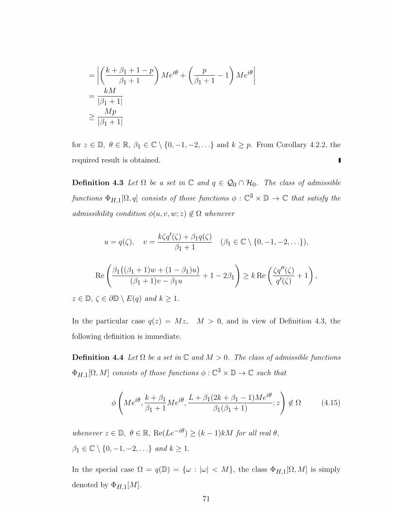
=
∣∣∣∣(k + β1 + 1− pβ1 + 1
)Meiθ +
(p
β1 + 1− 1
)Meiθ
∣∣∣∣=
kM
|β1 + 1|
≥ Mp
|β1 + 1|
for z ∈ D, θ ∈ R, β1 ∈ C \ 0,−1,−2, . . . and k ≥ p. From Corollary 4.2.2, the
required result is obtained.
Definition 4.3 Let Ω be a set in C and q ∈ Q0 ∩ H0. The class of admissible
functions ΦH,1[Ω, q] consists of those functions φ : C3 × D → C that satisfy the
admissibility condition φ(u, v, w; z) 6∈ Ω whenever
u = q(ζ), v =kζq′(ζ) + β1q(ζ)
β1 + 1(β1 ∈ C \ 0,−1,−2, . . .),
Re
(β1((β1 + 1)w + (1− β1)u
)(β1 + 1)v − β1u
+ 1− 2β1
)≥ kRe
(ζq′′(ζ)
q′(ζ)+ 1
),
z ∈ D, ζ ∈ ∂D \ E(q) and k ≥ 1.
In the particular case q(z) = Mz, M > 0, and in view of Definition 4.3, the
following definition is immediate.
Definition 4.4 Let Ω be a set in C and M > 0. The class of admissible functions
ΦH,1[Ω,M ] consists of those functions φ : C3 × D→ C such that
φ
(Meiθ,
k + β1
β1 + 1Meiθ,
L+ β1(2k + β1 − 1)Meiθ
β1(β1 + 1); z
)6∈ Ω (4.15)
whenever z ∈ D, θ ∈ R, Re(Le−iθ) ≥ (k − 1)kM for all real θ,
β1 ∈ C \ 0,−1,−2, . . . and k ≥ 1.
In the special case Ω = q(D) = ω : |ω| < M, the class ΦH,1[Ω,M ] is simply
denoted by ΦH,1[M ].
71

Theorem 4.5 Let φ ∈ ΦH,1[Ω, q] and β1 ∈ C\0,−1,−2, . . .. If f ∈ Ap satisfies
φ
(Hl,mp [β1 + 2]f(z)
zp−1,Hl,mp [β1 + 1]f(z)
zp−1,Hl,mp [β1]f(z)
zp−1; z
): z ∈ D
⊂ Ω,
(4.16)
then
Hl,mp [β1 + 2]f(z)
zp−1≺ q(z).
Proof. Define the analytic function p in D by
p(z) :=Hl,mp [β1 + 2]f(z)
zp−1. (4.17)
A computation shows that
z(Hl,mp [β1 + 2]f(z)
)′= (p− 1)zp−1p(z) + zpp′(z). (4.18)
By replacing (4.18) in (4.6), it follows that
(β1 + 1)Hl,mp [β1 + 1]f(z)
= (p− 1)zp−1p(z) + zpp′(z) + (β1 + 1− p)H l,mp [β1 + 2]f(z).
Hence,
Hl,mp [β1 + 1]f(z)
zp−1=zp′(z) + β1p(z)
β1 + 1. (4.19)
From (4.19), it follows that
Hl,mp [β1 + 1]f(z) =
zpp′(z) + β1zp−1p(z)
β1 + 1
and
(Hl,mp [β1 + 1]f(z))′
=1
β1 + 1
(pzp−1p′(z) + zpp′′(z) + β1(p− 1)zp−2p(z) + β1z
p−1p′(z))
72
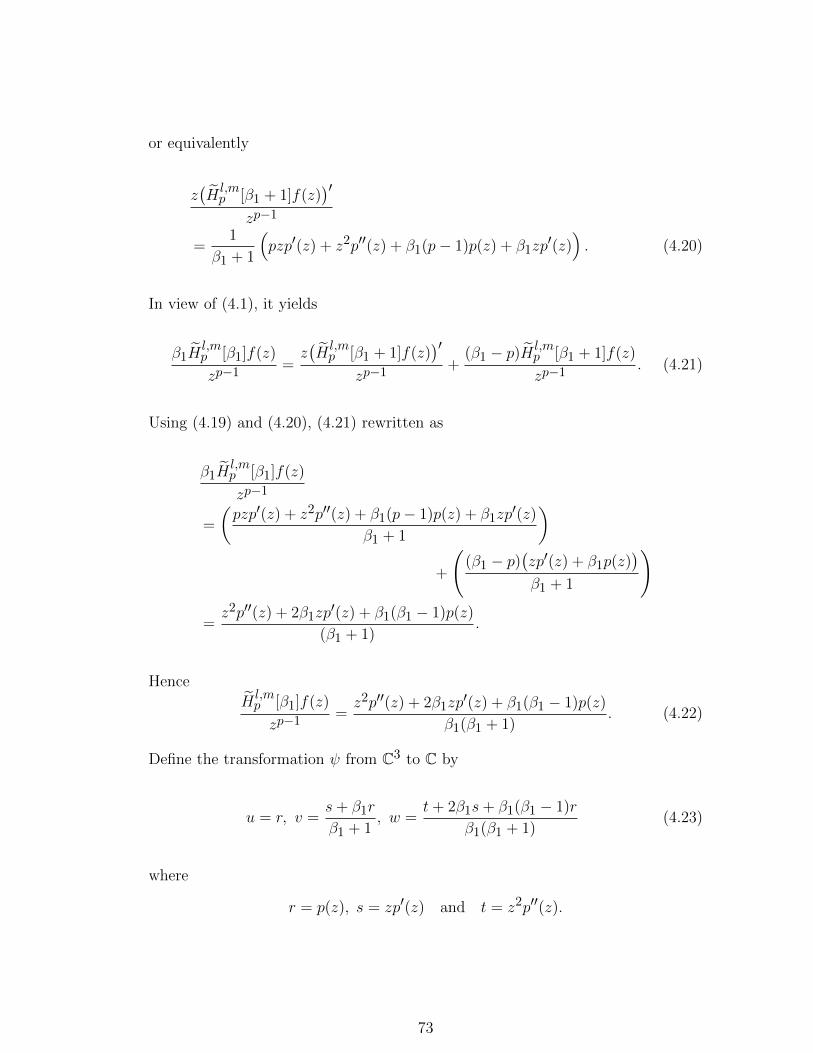
or equivalently
z(Hl,mp [β1 + 1]f(z)
)′zp−1
=1
β1 + 1
(pzp′(z) + z2p′′(z) + β1(p− 1)p(z) + β1zp
′(z)). (4.20)
In view of (4.1), it yields
β1Hl,mp [β1]f(z)
zp−1=z(Hl,mp [β1 + 1]f(z)
)′zp−1
+(β1 − p)H
l,mp [β1 + 1]f(z)
zp−1. (4.21)
Using (4.19) and (4.20), (4.21) rewritten as
β1Hl,mp [β1]f(z)
zp−1
=
(pzp′(z) + z2p′′(z) + β1(p− 1)p(z) + β1zp
′(z)
β1 + 1
)+
((β1 − p)
(zp′(z) + β1p(z)
)β1 + 1
)
=z2p′′(z) + 2β1zp
′(z) + β1(β1 − 1)p(z)
(β1 + 1).
Hence
Hl,mp [β1]f(z)
zp−1=z2p′′(z) + 2β1zp
′(z) + β1(β1 − 1)p(z)
β1(β1 + 1). (4.22)
Define the transformation ψ from C3 to C by
u = r, v =s+ β1r
β1 + 1, w =
t+ 2β1s+ β1(β1 − 1)r
β1(β1 + 1)(4.23)
where
r = p(z), s = zp′(z) and t = z2p′′(z).
73

Let
ψ(r, s, t; z) = φ(u, v, w; z) = φ
(r,s+ β1r
β1 + 1,t+ 2β1s+ β1(β1 − 1)r
β1(β1 + 1); z
). (4.24)
From (4.17), (4.19) and (4.22), equation (4.24), leads to
ψ(p(z), zp′(z), z2p′′(z); z
)= φ
(Hl,mp [β1 + 2]f(z)
zp−1,Hl,mp [β1 + 1]f(z)
zp−1,Hl,mp [β1]f(z)
zp−1; z
). (4.25)
Hence (4.16) becomes
ψ(p(z), zp′(z), z2p′′(z); z
)∈ Ω.
To complete the proof the admissibility condition for φ ∈ ΦH,1[Ω, q] is shown to
be equivalent to the admissibility condition for ψ as given in Definition 2.1. Note
that
v =s+ β1r
β1 + 1
implies
s = v(β1 + 1)− β1r.
A computation from
w =t+ 2β1s+ β1(β1 − 1)r
β1(β1 + 1)
shows that
t
s+ 1 =
wβ1(β1 + 1)− β1(β1 − 1)u
v(β1 + 1)− β1u+ 1− 2β1 (u = r).
74
Hence ψ ∈ Ψ[Ω, q]. By Theorem 2.1, p(z) ≺ q(z) or
Hl,mp [β1 + 2]f(z)
zp−1≺ q(z).
As in the previous case, if Ω 6= C is a simply connected domain, then Ω = h(D)
for some conformal mapping h of D onto Ω. In this case, the class ΦH,1[h(D), q] is
written as ΦH,1[h, q]. The following result is an immediate consequence of Theorem
4.5.
Theorem 4.6 Let φ ∈ ΦH,1[h, q] and β1 ∈ C\0,−1,−2, . . .. If f ∈ Ap satisfies
φ
(Hl,mp [β1 + 2]f(z)
zp−1,Hl,mp [β1 + 1]f(z)
zp−1,Hl,mp [β1]f(z)
zp−1; z
)≺ h(z),
then
Hl,mp [β1 + 2]f(z)
zp−1≺ q(z).
Corollary 4.2.5 Let φ ∈ ΦH,1[Ω,M ] and β1 ∈ C \ 0,−1,−2, . . .. If f ∈ Ap
satisfies
φ
(Hl,mp [β1 + 2]f(z)
zp−1,Hl,mp [β1 + 1]f(z)
zp−1,Hl,mp [β1]f(z)
zp−1; z
)∈ Ω,
then ∣∣∣∣∣Hl,mp [β1 + 2]f(z)
zp−1
∣∣∣∣∣ < M.
Proof. The result follows by taking q(z) = Mz in Theorem 4.5.
Corollary 4.2.6 Let φ ∈ ΦH,1[M ] and β1 ∈ C \ 0,−1,−2, . . .. If f ∈ Ap
satisfies
∣∣∣∣∣φ(Hl,mp [β1 + 2]f(z)
zp−1,Hl,mp [β1 + 1]f(z)
zp−1,Hl,mp [β1]f(z)
zp−1; z
)∣∣∣∣∣ < M,
75

then ∣∣∣∣∣Hl,mp [β1 + 2]f(z)
zp−1
∣∣∣∣∣ < M.
Proof. By taking Ω = q(D) in Corollary 4.2.5, the result is obtained.
Taking φ(u, v, w; z) = v in Corollary 4.2.6 leads to the following example.
Example 4.2 If Re β1 ≥ −1 and f ∈ Ap satisfies
∣∣∣∣∣Hl,mp [β1 + 1]f(z)
zp−1
∣∣∣∣∣ < M,
then ∣∣∣∣∣Hl,mp [β1 + 2]f(z)
zp−1
∣∣∣∣∣ < M.
Proof. By taking φ(u, v, w; z) in Corollary 4.2.6, we have to find the condition so
that φ ∈ ΦH,1[M ], that is, the admissibility condition (4.15) is satisfied. This
follows
∣∣∣∣∣φ(Meiθ,
k + β1
β1 + 1Meiθ,
L+ β1(2k + β1 − 1)Meiθ
β1(β1 + 1); z
)∣∣∣∣∣ ≥M
which implies
∣∣∣∣k + β1
β1 + 1Meiθ
∣∣∣∣ ≥M
or
|k + β1| ≥ |β1 + 1|. (4.26)
Following inequality (4.26), a computation shows that
Re β1 ≥−(1 + k)
2.
76

Since k ≥ 1, then it is sufficient to write
Re β1 ≥ −1
for (4.26) holds true. Hence, from Corollary 4.2.6, if Re β1 ≥ −1 and
∣∣∣∣∣Hl,mp [β1 + 1]f(z)
zp−1
∣∣∣∣∣ < M,
then ∣∣∣∣∣Hl,mp [β1 + 2]f(z)
zp−1
∣∣∣∣∣ < M.
This completes the proof.
Remark 4.2.1 The analogue of Corollary 4.2.3 and Corollary 4.2.6 can be ob-
tained by choosing suitable admissible function.
Definition 4.5 Let Ω be a set in C and q ∈ Q1 ∩ H. The class of admissible
functions ΦH,2[Ω, q] consists of those functions φ : C3 × D → C that satisfy the
admissibility condition φ(u, v, w; z) 6∈ Ω whenever
u = q(ζ), v =(β1 + 1)q(ζ)
(β1 + 2)− kζq′(ζ)− q(ζ), (β1 ∈ C \ 0,−1,−2, . . ., q(ζ) 6= 0),
Re
((β + 1)u
v(β + 2)− (β + 1)u− vu
(β + 1
v− β
w− 1
)− β + 1
v− 1
)≥ kRe
(ζq′′(ζ)
q′(ζ)+ 1
),
z ∈ D, ζ ∈ ∂D \ E(q) and k ≥ 1.
In the particular case q(z) = 1 + Mz, M > 0, and in view of Definition 4.5, the
following definition is immediate.
Definition 4.6 Let Ω be a set in C and M > 0. The class of admissible functions
ΦH,2[Ω,M ] consists of those functions φ : C3 × D→ C such that
77

φ
(1 +Meiθ,
(β1 + 1)(1 +Meiθ)
(β1 + 1)−Meiθ(k + 1),
β1(1 +Meiθ)(β1 + 1−Meiθ(k + 1)
)(β1 + 1−Meiθ(k + 1)
)(β1 − 2Meiθ(k + 1)
)− (1 +Meiθ)(L+ 2Meiθ)
; z
)6∈ Ω
whenever z ∈ D, θ ∈ R,
Re
(((β1 + 1)−Meiθ(k + 1)
)(1− kMeiθ)− L(1 +Meiθ)
kMeiθ(1 +Meiθ)
)≥ (k + 4)
for all real θ, β1 ∈ C \ 0,−1,−2, . . . and k ≥ 1.
In the special case Ω = q(D) = ω : |ω − 1| < M, the class ΦH,2[Ω,M ] is simply
denoted by ΦH,2[M ].
Theorem 4.7 Let φ ∈ ΦH,2[Ω, q] and β1 ∈ C\0,−1,−2, . . .. If f ∈ Ap satisfies
φ
(Hl,mp [β1 + 3]f(z)
Hl,mp [β1 + 2]f(z)
,Hl,mp [β1 + 2]f(z)
Hl,mp [β1 + 1]f(z)
,Hl,mp [β1 + 1]f(z)
Hl,mp [β1]f(z)
; z
): z ∈ D
⊂ Ω,
(4.27)
then
Hl,mp [β1 + 3]f(z)
Hl,mp [β1 + 2]f(z)
≺ q(z).
Proof. Define the analytic function p in D by
p(z) :=Hl,mp [β1 + 3]f(z)
Hl,mp [β1 + 2]f(z)
. (4.28)
By using (4.28), a computation shows that get
zp′(z)
p(z)=z(Hl,mp [β1 + 3]f(z)
)′Hl,mp [β1 + 3]f(z)
−z(Hl,mp [β1 + 2]f(z)
)′Hl,mp [β1 + 2]f(z)
. (4.29)
78
In view of the relation (4.1), it follows that
(β1 + 2)Hl,mp [β1 + 2]f(z) = z
(Hl,mp [β1 + 3]f(z)
)′+ (β1 + 2− p)H l,m
p [β1 + 3]f(z).
(4.30)
Using (4.6) and (4.30), (4.29) can be written as
zp′(z)
p(z)=
(β1 + 2)Hl,mp [β1 + 2]f(z)− (β1 + 2− p)H l,m
p [β1 + 3]f(z)
Hl,mp [β1 + 3]f(z)
−
((β1 + 1)H
l,mp [β1 + 1]f(z)− (β1 + 1− p)H l,m
p [β1 + 2]f(z)
Hl,mp [β1 + 2]f(z)
)
=(β1 + 2)H
l,mp [β1 + 2]f(z)
Hl,mp [β1 + 3]f(z)
−(β1 + 1)H
l,mp [β1 + 1]f(z)
Hl,mp [β1 + 2]f(z)
− 1.
By (4.28), it follows that
(β1 + 1)Hl,mp [β1 + 1]f(z)
Hl,mp [β1 + 2]f(z)
=(β1 + 2)
p(z)− zp′(z)
p(z)− 1
=(β1 + 2)− zp′(z)− p(z)
p(z)
or
Hl,mp [β1 + 1]f(z)
Hl,mp [β1 + 2]f(z)
=(β1 + 2)− zp′(z)− p(z)
(β1 + 1)p(z).
Hence,
Hl,mp [β1 + 2]f(z)
Hl,mp [β1 + 1]f(z)
=(β1 + 1)p(z)
(β1 + 2)− zp′(z)− p(z). (4.31)
Further computations show that
z
(H l,m
p [β1+2]f(z)
Hl,mp [β1+1]f(z)
)′(H l,m
p [β1+2]f(z)
H l,mp [β1+1]f(z)
) =z(Hl,mp [β1 + 2]f(z)
)′Hl,mp [β1 + 2]f(z)
−z(Hl,mp [β1 + 1]f(z)
)′Hl,mp [β1 + 1]f(z)
(4.32)
79

Using (4.1) and (4.6), (4.32) can be written as
z
(H
l,mp [β1+2]f(z)
H l,mp [β1+1]f(z)
)′(H l,m
p [β1+2]f(z)
H l,mp [β1+1]f(z)
) =(β1 + 1)H
l,mp [β1 + 1]f(z)− (β1 + 1− p)H l,m
p [β1 + 2]f(z)
Hl,mp [β1 + 2]f(z)
−
(β1H
l,mn β1f(z)− (β1 − p)H
l,mp [β1 + 1]f(z)
Hl,mp [β1 + 1]f(z)
)
=(β1 + 1)H
l,mp [β1 + 1]f(z)
Hl,mp [β1 + 2]f(z)
− β1Hl,mn β1f(z)
Hl,mp [β1 + 1]f(z)
− 1,
or
β1Hl,mn β1f(z)
Hl,mp [β1 + 1]f(z)
=(β1 + 1)H
l,mp [β1 + 1]f(z)
Hl,mp [β1 + 2]f(z)
−z
(H l,m
p [β1+2]f(z)
H l,mp [β1+1]f(z)
)′(H l,m
p [β1+2]f(z)
H l,mp [β1+1]f(z)
) − 1.
(4.33)
Further computation shows that
(Hl,mp [β1 + 2]f(z)
Hl,mp [β1 + 1]f(z)
)′
=(β1 + 1)p′(z)
((β1 + 2)− zp′(z)− p(z)
)−(− zp′′(z)− 2p′(z)
)((β1 + 1)p(z)
)((β1 + 2)− zp′(z)− p(z)
)2and
(H l,m
p [β1+2]f(z)
Hl,mp [β1+1]f(z)
)′(H l,m
p [β1+2]f(z)
H l,mp [β1+1]f(z)
) =p′(z)
p(z)+
zp′′(z) + 2p′(z)
(β1 + 2)− zp′(z)− p(z).
80

Hence
z
(H
l,mp [β1+2]f(z)
H l,mp [β1+1]f(z)
)′(H l,m
p [β1+2]f(z)
H l,mp [β1+1]f(z)
) =zp′(z)
p(z)+
z2p′′(z) + 2zp′(z)
(β1 + 2)− zp′(z)− p(z)(4.34)
Using (4.31) and (4.34), (4.33) can be written as
β1Hl,mp [β1]f(z)
Hl,mp [β1 + 1]f(z)
=(β1 + 2)− zp′(z)− p(z)
p(z)− zp′(z)
p(z)
−(
z2p′′(z) + 2zp′(z)
(β1 + 2)− zp′(z)− p(z)
)− 1
which implies
Hl,mp [β1 + 1]f(z)
Hl,mp [β1]f(z)
=β1
β1−2−zp′(z)−p(z)p(z)
− zp′(z)p(z)
−(z2p′′(z)+2zp′(z)
)β1+2−zp′(z)−p(z) − 1
. (4.35)
Define the transformation ψ from C3 to C by
u = r, v =(β1 + 1)r
β1 + 2− s− r, w =
β1
β1+2−s−rr − s
r −(t+2s)
β1+2−s−r − 1, (4.36)
where
r = p(z), s = zp′(z) and t = z2p′′(z).
Let
ψ(r, s, t; z) := φ(u, v, w; z)
= φ
r, (β1 + 1)r
β1 + 2− s− r,
β1
β1+2−s−rr − s
r −(t+2s)
β1+2−s−r − 1; z
. (4.37)
81

From (4.28), (4.31) and (4.35), the equation(4.37), yields
ψ(p(z), zp′(z), z2p′′(z); z
)= φ
(Hl,mp [β1 + 3]f(z)
Hl,mp [β1 + 2]f(z)
,Hl,mp [β1 + 2]f(z)
Hl,mp [β1 + 1]f(z)
,Hl,mp [β1 + 1]f(z)
Hl,mp [β1]f(z)
; z
). (4.38)
Hence (4.27) becomes
ψ(p(z), zp′(z), z2p′′(z); z
)∈ Ω.
To complete the proof the admissibility condition for φ ∈ ΦH,2[Ω, q] is shown to
be equivalent to the admissibility condition for ψ as given in Definition 2.1. Note
that
v =(β1 + 1)r
β1 + 2− s− r
implies
s =v(β1 + 2)− (β1 + 1)r − rv
v. (4.39)
By using (4.39) in
w =β1
β1+2−s−rr − s
r −(t+2s)
β1+2−s−r − 1,
a computation shows that
t
s+ 1 =
(β1 + 1)u
v(β1 + 2)− (β1 + 1)u− vu
(β1 + 1
v− β1
w− 1
)− β1 + 1
v− 1 (u = r)
(4.40)
and hence ψ ∈ Ψ[Ω, q]. By Theorem 2.1, p(z) ≺ q(z) or
Hl,mp [β1 + 3]f(z)
Hl,mp [β1 + 2]f(z)
≺ q(z).
82

As in the previous cases, if Ω 6= C is a simply connected domain, then Ω = h(D)
for some conformal mapping h of D onto Ω. In this case the class ΦH,2[h(D), q] is
written as ΦH,2[h, q]. The following result is an immediate consequence of Theorem
4.7.
Theorem 4.8 Let φ ∈ ΦH,2[h, q] and β1 ∈ C\0,−1,−2, . . .. If f ∈ Ap satisfies
φ
(Hl,mp [β1 + 3]f(z)
Hl,mp [β1 + 2]f(z)
,Hl,mp [β1 + 2]f(z)
Hl,mp [β1 + 1]f(z)
,Hl,mp [β1 + 1]f(z)
Hl,mp [β1]f(z)
; z
)≺ h(z),
then
Hl,mp [β1 + 3]f(z)
Hl,mp [β1 + 2]f(z)
≺ q(z).
Corollary 4.2.7 Let φ ∈ ΦH,2[Ω,M ] and β1 ∈ C \ 0,−1,−2, . . .. If f ∈ Ap
satisfies
φ
(Hl,mp [β1 + 3]f(z)
Hl,mp [β1 + 2]f(z)
,Hl,mp [β1 + 2]f(z)
Hl,mp [β1 + 1]f(z)
,Hl,mp [β1 + 1]f(z)
Hl,mp [β1]f(z)
; z
)∈ Ω,
then ∣∣∣∣∣Hl,mp [β1 + 3]f(z)
Hl,mp [β1 + 2]f(z)
− 1
∣∣∣∣∣ < M.
Proof. The result follows by taking q(z) = 1 +Mz in Theorem 4.7.
Corollary 4.2.8 Let φ ∈ ΦH,2[M ] and β1 ∈ C \ 0,−1,−2, . . .. If f ∈ Ap
satisfies
∣∣∣∣∣φ(Hl,mp [β1 + 3]f(z)
Hl,mp [β1 + 2]f(z)
,Hl,mp [β1 + 2]f(z)
Hl,mp [β1 + 1]f(z)
,Hl,mp [β1 + 1]f(z)
Hl,mp [β1]f(z)
; z
)− 1
∣∣∣∣∣ < M,
then ∣∣∣∣∣Hl,mp [β1 + 3]f(z)
Hl,mp [β1 + 2]f(z)
− 1
∣∣∣∣∣ < M.
Proof. By taking Ω = q(D) in Corollary 4.2.7, the result is obtained.
83

4.3 Superordination of the Dziok-Srivastava Operator
The dual problem of differential subordination, that is, differential superordination
of the Dziok-Srivastava linear operator is investigated in this section. For this
purpose, the following class of admissible functions will be required.
Definition 4.7 Let Ω be a set in C and q ∈ H[0, p] with zq′(z) 6= 0. The class
of admissible functions Φ′H [Ω, q] consists of those functions φ : C3 × D → C that
satisfy the admissibility condition φ(u, v, w; ζ) ∈ Ω whenever
u = q(z), v =zq′(z) +m(β1 + 1− p)q(z)
m(β1 + 1)(β1 ∈ C \ 0,−1,−2, . . .),
Re
(β1(β1 + 1)w + (p− β1)(β1 − p+ 1)u
(β1 + 1)v + (p− β1 − 1)u− (2(β1 − p) + 1)
)≤ 1
mRe
(zq′′(z)
q′(z)+ 1
),
z ∈ D, ζ ∈ ∂D and m ≥ p.
Theorem 4.9 Let φ ∈ Φ′H [Ω, q] and β1 ∈ C \ 0,−1,−2, . . .. If f ∈ Ap,
Hl,mp [β1 + 2]f(z) ∈ Q0 and
φ(Hl,mp [β1 + 2]f(z), H
l,mp [β1 + 1]f(z), H
l,mp [β1]f(z); z
)
is univalent in D, then
Ω ⊂φ(Hl,mp [β1 + 2]f(z), H
l,mp [β1 + 1]f(z), H
l,mp [β1]f(z); z
): z ∈ D
(4.41)
implies
q(z) ≺ Hl,mp [β1 + 2]f(z).
Proof. From (4.11) and (4.41), it follows that
Ω ⊂ψ(p(z), zp′(z), z2p′′(z); z
): z ∈ D
.
84

From (4.9), it is clear that the admissibility condition for φ ∈ Φ′H [Ω, q] is equivalent
to the admissibility condition for ψ as given in Definition 2.2. Hence ψ ∈ Ψ′p[Ω, q],
and by Theorem 2.2, q(z) ≺ p(z) or
q(z) ≺ Hl,mp [β1 + 2]f(z).
If Ω 6= C is a simply connected domain, then Ω = h(D) for some conformal
mapping h of D onto Ω. In this case the class Φ′H [h(D), q] is written as Φ′H [h, q].
Proceeding similarly as in the previous section, the following result is an immediate
consequence of Theorem 4.9.
Theorem 4.10 Let h be analytic in D, φ ∈ Φ′H [h, q] and β1 ∈ C\0,−1,−2, . . ..
If f ∈ Ap, Hl,mp [β1 + 2]f(z) ∈ Q0 and
φ(Hl,mp [β1 + 2]f(z), H
l,mp [β1 + 1]f(z), H
l,mp [β1]f(z); z
)
is univalent in D, then
h(z) ≺ φ(Hl,mp [β1 + 2]f(z), H
l,mp [β1 + 1]f(z), H
l,mp [β1]f(z); z
)(4.42)
implies
q(z) ≺ Hl,mp [β1 + 2]f(z).
Theorem 4.9 and 4.10 can only be used to obtain subordinants of differential
superordination of the form (4.41) or (4.42). The following theorem proves the
existence of the best subordinant of (4.42) for certain φ.
Theorem 4.11 Let h be analytic in D, φ : C3×D→ C and β1 ∈ C\0,−1,−2, . . ..
Suppose that the differential equation
φ(q(z), zq′(z), z2q′′(z); z
)= h(z) (4.43)
85
has a solution q ∈ Q0. If φ ∈ Φ′H [h, q], f ∈ Ap, Hl,mp [β1 + 2]f(z) ∈ Q0 and
φ(Hl,mp [β1 + 2]f(z), H
l,mp [β1 + 1]f(z), H
l,mp [β1]f(z); z
)
is univalent in D, then
h(z) ≺ φ(Hl,mp [β1 + 2]f(z), H
l,mp [β1 + 1]f(z), H
l,mp [β1]f(z); z
)
implies
q(z) ≺ Hl,mp [β1 + 2]f(z)
and q is the best subordinant.
Proof. In view of Theorem 4.9 and Theorem 4.10 we deduce that q is a subordinant
of (4.42). Since q satisfies (4.43), it is also a solution of (4.42) and therefore q will
be subordinated by all subordinants. Hence q is the best subordinant.
Combining Theorems 4.2 and 4.10, we obtain the following sandwich-type
theorem.
Corollary 4.3.1 Let h1 and q1 be analytic functions in D, h2 be univalent function
in D, q2 ∈ Q0 with q1(0) = q2(0) = 0, φ ∈ ΦH [h2, q2] ∩ Φ′H [h1, q1] and β1 ∈
C \ 0,−1,−2, . . .. If f ∈ Ap, Hl,mp [β1 + 2]f(z) ∈ H[0, p] ∩Q0 and
φ(Hl,mp [β1 + 2]f(z), H
l,mp [β1 + 1]f(z), H
l,mp [β1]f(z); z
)
is univalent in D, then
h1(z) ≺ φ(Hl,mp [β1 + 2]f(z), H
l,mp [β1 + 1]f(z), H
l,mp [β1]f(z); z
)≺ h2(z),
86

implies
q1(z) ≺ Hl,mp [β1 + 2]f(z) ≺ q2(z).
Definition 4.8 Let Ω be a set in C and q ∈ H0 with zq′(z) 6= 0. The class of
admissible functions Φ′H,1[Ω, q] consists of those functions φ : C3 × D → C that
satisfy the admissibility condition φ(u, v, w; ζ) ∈ Ω whenever
u = q(z), v =zq′(z) +mβ1q(z)
m(β1 + 1)(β1 ∈ C \ 0,−1,−2, . . .),
Re
(β1((β1 + 1)w + (1− β1)u
)(β1 + 1)v − β1u
+ 1− 2β1
)≤ 1
mRe
(zq′′(z)
q′(z)+ 1
),
z ∈ D, ζ ∈ ∂D and m ≥ 1.
Next, the dual result of Theorem 4.5 for differential superordination will be
given.
Theorem 4.12 Let φ ∈ Φ′H,1[Ω, q] and β1 ∈ C \ 0,−1,−2, . . .. If f ∈ Ap,H l,m
p [β1+2]f(z)
zp−1∈ Q0 and
φ
(Hl,mp [β1 + 2]f(z)
zp−1,Hl,mp [β1 + 1]f(z)
zp−1,Hl,mp [β1]f(z)
zp−1; z
)
is univalent in D, then
Ω ⊂
φ
(Hl,mp [β1 + 2]f(z)
zp−1,Hl,mp [β1 + 1]f(z)
zp−1,Hl,mp [β1]f(z)
zp−1; z
): z ∈ D
(4.44)
implies
q(z) ≺Hl,mp [β1 + 2]f(z)
zp−1.
Proof. From (4.25) and (4.44), it follows that
Ω ⊂φ(p(z), zp′(z), z2p′′(z); z
): z ∈ D
87

From (4.23), it follows that the admissibility condition for φ ∈ Φ′H,1[Ω, q] is
equivalent to the admissibility condition for ψ as given in Definition 2.2. Hence
ψ ∈ Ψ′[Ω, q], and by Theorem 2.2, q(z) ≺ p(z) or
q(z) ≺Hl,mp [β1 + 2]f(z)
zp−1.
If Ω 6= C is a simply connected domain, then Ω = h(D) for some conformal
mapping h of D onto Ω. In this case the class Φ′H,1[h(D), q] is written as Φ′H,1[h, q].
The following result is an immediate consequence of Theorem 4.12.
Theorem 4.13 Let q ∈ H0, h be analytic on D, φ ∈ Φ′H,1[h, q] and β1 ∈ C \
0,−1,−2, . . .. If f ∈ Ap,H
l,mp [β1+2]f(z)
zp−1∈ Q0 and
φ
(Hl,mp [β1 + 2]f(z)
zp−1,Hl,mp [β1 + 1]f(z)
zp−1,Hl,mp [β1]f(z)
zp−1; z
)
is univalent in D, then
h(z) ≺ φ
(Hl,mp [β1 + 2]f(z)
zp−1,Hl,mp [β1 + 1]f(z)
zp−1,Hl,mp [β1]f(z)
zp−1; z
)
implies
q(z) ≺Hl,mp [β1 + 2]f(z)
zp−1.
Combining Theorems 4.6 and 4.13, the following sandwich-type theorem is
obtained.
Corollary 4.3.2 Let h1 and q1 be analytic functions in D, h2 be univalent func-
tion in D, q2 ∈ Q0 with q1(0) = q2(0) = 0, φ ∈ ΦH,1[h2, q2] ∩ Φ′H,1[h1, q1] and
β1 ∈ C \ 0,−1,−2, . . .. If f ∈ Ap,H l,m
p [β1+2]f(z)
zp−1∈ H0 ∩Q0 and
φ
(Hl,mp [β1 + 2]f(z)
zp−1,Hl,mp [β1 + 1]f(z)
zp−1,Hl,mp [β1]f(z)
zp−1; z
)88
is univalent in D, then
h1(z) ≺ φ
(Hl,mp [β1 + 2]f(z)
zp−1,Hl,mp [β1 + 1]f(z)
zp−1,Hl,mp [β1]f(z)
zp−1; z
)≺ h2(z),
implies
q1(z) ≺Hl,mp [β1 + 2]f(z)
zp−1≺ q2(z).
Definition 4.9 Let Ω be a set in C, q(z) 6= 0, zq′(z) 6= 0 and q ∈ H. The class
of admissible functions Φ′H,2[Ω, q] consists of those functions φ : C3×D→ C that
satisfy the admissibility condition φ(u, v, w; ζ) ∈ Ω whenever
u = q(z), v =m(β1 + 1)q(z)
m(β1 + 2)− zq′(z)−mq(z), (β1 ∈ C\0,−1,−2, . . ., q(z) 6= 0),
Re
(β1u(β1 + 1)(w − 1)
w((β1 + 1)(v − u) + v(1− u)
) − (β + 1)
v− 1
)≤ 1
mRe
(zq′′(z)
q′(z)+ 1
),
z ∈ D, ζ ∈ ∂D and m ≥ 1.
Now, the dual result of Theorem 4.7 for differential superordination will be
given.
Theorem 4.14 Let φ ∈ Φ′H,2[Ω, q] and β1 ∈ C \ 0,−1,−2, . . .. If f ∈ Ap,
Hl,mp [β1+3]f(z)
H l,mp [β1+2]f(z)
∈ Q1 and
φ
(Hl,mp [β1 + 3]f(z)
Hl,mp [β1 + 2]f(z)
,Hl,mp [β1 + 2]f(z)
Hl,mp [β1 + 1]f(z)
,Hl,mp [β1 + 1]f(z)
Hl,mp [β1]f(z)
; z
)
is univalent in D, then
Ω ⊂
φ
(Hl,mp [β1 + 3]f(z)
Hl,mp [β1 + 2]f(z)
,Hl,mp [β1 + 2]f(z)
Hl,mp [β1 + 1]f(z)
,Hl,mp [β1 + 1]f(z)
Hl,mp [β1]f(z)
; z
): z ∈ D
(4.45)
89
implies
q(z) ≺Hl,mp [β1 + 3]f(z)
Hl,mp [β1 + 2]f(z)
.
Proof. From (4.38) and (4.45), it follows that
Ω ⊂φ(p(z), zp′(z), z2p′′(z); z
): z ∈ D
.
In view of (4.36), the admissibility condition for φ ∈ Φ′H,2[Ω, q] is equivalent to
the admissibility condition for ψ as given in Definition 2.2. Hence ψ ∈ Ψ′[Ω, q],
and by Theorem 2.2, q(z) ≺ p(z) or
q(z) ≺Hl,mp [β1 + 3]f(z)
Hl,mp [β1 + 2]f(z)
.
If Ω 6= C is a simply connected domain, then Ω = h(D) for some conformal
mapping h of D onto Ω. In this case the class Φ′H,2[h(D), q] is written as Φ′H,2[h, q].
Proceeding similarly as in the previous section, the following result is an immediate
consequence of Theorem 4.14.
Theorem 4.15 Let q ∈ H, h be analytic in D, φ ∈ Φ′H,2[h, q] and β1 ∈ C \
0,−1,−2, . . .. If f ∈ Ap,H l,m
p [β1+3]f(z)
Hl,mp [β1+2]f(z)
∈ Q1 and
φ
(Hl,mp [β1 + 3]f(z)
Hl,mp [β1 + 2]f(z)
,Hl,mp [β1 + 2]f(z)
Hl,mp [β1 + 1]f(z)
,Hl,mp [β1 + 1]f(z)
Hl,mp [β1]f(z)
; z
)
is univalent in D, then
h(z) ≺ φ
(Hl,mp [β1 + 3]f(z)
Hl,mp [β1 + 2]f(z)
,Hl,mp [β1 + 2]f(z)
Hl,mp [β1 + 1]f(z)
,Hl,mp [β1 + 1]f(z)
Hl,mp [β1]f(z)
; z
)
implies
q(z) ≺Hl,mp [β1 + 3]f(z)
Hl,mp [β1 + 2]f(z)
.
90

Combining Theorems 4.8 and 4.15 yield the following sandwich-type theorem.
Corollary 4.3.3 Let h1 and q1 be analytic functions in D, h2 be univalent func-
tion in D, q2 ∈ Q1 with q1(0) = q2(0) = 1, φ ∈ ΦH,2[h2, q2] ∩ Φ′H,2[h1, q1] and
β1 ∈ C \ 0,−1,−2, . . .. If f ∈ Ap,H l,m
p [β1+3]f(z)
H l,mp [β1+2]f(z)
∈ H ∩Q1 and
φ
(Hl,mp [β1 + 3]f(z)
Hl,mp [β1 + 2]f(z)
,Hl,mp [β1 + 2]f(z)
Hl,mp [β1 + 1]f(z)
,Hl,mp [β1 + 1]f(z)
Hl,mp [β1]f(z)
; z
)
is univalent in D, then
h1(z) ≺ φ
(Hl,mp [β1 + 3]f(z)
Hl,mp [β1 + 2]f(z)
,Hl,mp [β1 + 2]f(z)
Hl,mp [β1 + 1]f(z)
,Hl,mp [β1 + 1]f(z)
Hl,mp [β1]f(z)
; z
)≺ h2(z),
implies
q1(z) ≺Hl,mp [β1 + 3]f(z)
Hl,mp [β1 + 2]f(z)
≺ q2(z).
4.4 Subordination of the Liu-Srivastava Operator
In this section, differential subordination results are obtained for multivalent mero-
morphic functions associated with the Liu-Srivastava linear operator in the punc-
tured unit disk. A similar problem was studied by Aghalary et al. [1,4], and related
results can be found in the works of [9,10,12–15,25,58,63]. The following class of
admissible functions will be required to obtain main results.
Definition 4.10 Let Ω be a set in C and q ∈ Q1 ∩ H. The class of admissible
functions ΦH [Ω, q] consists of those functions φ : C3 × D → C satisfying the
admissibility condition φ(u, v, w; z) 6∈ Ω whenever
u = q(ζ), v =kζq′(ζ) + (β1 + 1)q(ζ)
β1 + 1(β1 ∈ C \ 0,−1,−2, . . .),
Re
(β1(w − u)
(v − u)− (2β1 + 1)
)≥ kRe
(ζq′′(ζ)
q′(ζ)+ 1
),
91

z ∈ D, ζ ∈ ∂D \ E(q) and k ≥ 1.
Choosing q(z) = 1 +Mz, M > 0, Definition 4.10 easily gives the following defini-
tion.
Definition 4.11 Let Ω be a set in C and M > 0. The class of admissible functions
ΦH [Ω,M ] consists of those functions φ : C3 × D→ C such that
φ
(1 +Meiθ, 1 +
k + β1 + 1
β1 + 1Meiθ, 1 +
L+ (β1 + 1)(2k + β1)Meiθ
β1(β1 + 1); z
)6∈ Ω
(4.46)
whenever z ∈ D, θ ∈ R, Re(Le−iθ) ≥ (k − 1)kM for all real θ,
β1 ∈ C \ 0,−1,−2, . . . and k ≥ 1.
In the special case Ω = q(D) = ω : |ω − 1| < M, the class ΦH [Ω,M ] is simply
denoted by ΦH [M ].
Theorem 4.16 Let φ ∈ ΦH [Ω, q] and β1 ∈ C \ 0,−1,−2, . . .. If f ∈ Mp
satisfies
φ
(zpH∗
l,mp [β1 + 2]f(z), zpH∗
l,mp [β1 + 1]f(z), zpH∗
l,mp [β1]f(z); z
): z ∈ D
⊂ Ω,
(4.47)
then
zpH∗l,mp [β1 + 2]f(z) ≺ q(z) (z ∈ D).
Proof. Define the analytic function p in D by
p(z) := zpH∗l,mp [β1 + 2]f(z). (4.48)
In view of the relation (4.2), it follows that
(β1 +1)H∗l,mp [β1 +1]f(z) = z
(H∗
l,mp [β1 +2]f(z)
)′+(β1 +1+p)H∗
l,mp [β1 +2]f(z).
(4.49)
92

Using (4.48), a computation from (4.49) shows that
(β1 + 1)H∗l,mp [β1 + 1]f(z) =
zp′(z)− p.p(z)
zp+
(β + 1 + p)p(z)
zp
or equivalently
zpH∗l,mp [β1 + 1]f(z) =
1
β1 + 1
((β1 + 1)p(z) + zp′(z)
). (4.50)
By using (4.50), further computations from (4.2) show that
β1H∗l,mp [β1]f(z) = z
((β1 + 1)p(z) + zp′(z)
(β1 + 1)zp
)′+(β1 +p)
((β1 + 1)p(z) + zp′(z)
(β1 + 1)zp
)
which implies
β1(β1 + 1)H∗l,mp [β1]f(z) =
z2p′′(z) + 2(β1 + 1)zp′(z) + β1(β1 + 1)p(z)
zp.
Hence
zpH∗l,mp [β1]f(z) =
1
β1(β1 + 1)
(z2p′′(z) + 2(β1 + 1)zp′(z)
)+ p(z). (4.51)
Define the transformation ψ from C3 to C by
u = r, v =s+ (β1 + 1)r
β1 + 1, w =
t+ 2(β1 + 1)s+ (β1)(β1 + 1)r
β1(β1 + 1)(4.52)
where
r = p(z), s = zp′(z) and t = z2p′′(z).
Let
ψ(r, s, t; z) = φ(u, v, w; z)
= φ
(r,s+ (β1 + 1)r
β1 + 1,t+ 2(β1 + 1)s+ (β1)(β1 + 1)r
β1(β1 + 1); z
). (4.53)
93
From (4.48), (4.50) and (4.51), equation (4.53) yields
ψ(p(z), zp′(z), z2p′′(z); z
)= φ
(zpH∗
l,mp [β1 + 2]f(z), zpH∗
l,mp [β1 + 1]f(z), zpH∗
l,mp [β1]f(z); z
). (4.54)
Hence (4.47) becomes
ψ(p(z), zp′(z), z2p′′(z); z) ∈ Ω.
To complete the proof, it is left to show that the admissibility condition for φ ∈
ΦH [Ω, q] is equivalent to the admissibility condition for ψ as given in Definition
2.1. Note that
v =s+ (β1 + 1)r
β1 + 1
implies
s = (β1 + 1)(v − r).
A computation from
w =t+ 2(β1 + 1)s+ (β1)(β1 + 1)r
β1(β1 + 1)
shows that
t
s+ 1 =
β1(w − u)
(v − u)− (2β1 + 1) (u = r)
and hence ψ ∈ Ψn[Ω, q]. By Theorem 2.1, p(z) ≺ q(z) or
zpH∗l,mp [β1 + 2]f(z) ≺ q(z).
94

If Ω 6= C is a simply connected domain, then Ω = h(D) for some conformal
mapping h of D onto Ω. In this case the class ΦH [h(D), q] is written as ΦH [h, q].
The following result is an immediate consequence of Theorem 4.16.
Theorem 4.17 Let φ ∈ ΦH [h, q] with q(0) = 1 and β1 ∈ C \ 0,−1,−2, . . .. If
f ∈Mp and satisfies
φ
(zpH∗
l,mp [β1 + 2]f(z), zpH∗
l,mp [β1 + 1]f(z), zpH∗
l,mp [β1]f(z); z
)≺ h(z),
(4.55)
then
zpH∗l,mp [β1 + 2]f(z) ≺ q(z).
The next result is an extension of Theorem 4.16 to the case where the behavior of
q on ∂D is not known.
Corollary 4.4.1 Let Ω ⊂ C, q be univalent in D and q(0) = 1. Let φ ∈ ΦH [Ω, qρ]
for some ρ ∈ (0, 1) where qρ(z) = q(ρz) and β1 ∈ C \ 0,−1,−2, . . .. If f ∈ Mp
and
φ
(zpH∗
l,mp [β1 + 2]f(z), zpH∗
l,mp [β1 + 1]f(z), zpH∗
l,mp [β1]f(z); z
)∈ Ω,
then
zpH∗l,mp [β1 + 2]f(z) ≺ q(z).
Proof. Theorem 4.16 yields zpH∗l,mp [β1 + 2]f(z) ≺ qρ(z). The result now follows
from the fact that qρ(z) ≺ q(z).
Theorem 4.18 Let h and q be univalent in D, with q(0) = 1, set qρ(z) = q(ρz)
and hρ(z) = h(ρz) and β1 ∈ C \ 0,−1,−2, . . .. Let φ : C3 × D → C satisfy one
of the following conditions:
1. φ ∈ ΦH [h, qρ] for some ρ ∈ (0, 1), or
95

2. there exists ρ0 ∈ (0, 1) such that φ ∈ ΦH [hρ, qρ] for all ρ ∈ (ρ0, 1).
If f ∈Mp satisfies (4.55), then
zpH∗l,mp [β1 + 2]f(z) ≺ q(z).
Proof. (1) The function qρ is univalent on D, and therefore E(qρ) is empty and
qρ ∈ Q. The class ΦH [h, qρ] is an admissible class and from Theorem 4.16 we
obtain
zpH∗l,mp [β1 + 2]f(z) ≺ qρ(z).
Since qρ ≺ q we deduce zpH∗l,mp [β1 + 2]f(z) ≺ q(z).
(2) From (4.54), it is evident that φ ∈ ΦH [hρ, qρ] implies ψ ∈ ΨH [hp, qp]. If we let
Pρ(z) = P (ρz), then
ψ(pρ(z), zp′ρ(z), z2p′′ρ(z); ρz
)= ψ
(p(ρz), ρzp′(ρz), ρ2z2p′′(ρz); ρz
)∈ hρ(D).
By using Thorem 2.1, with ρz, a function mapping D into D we obtain
pρ(z) ≺ qρ(z), for ρ ∈ (ρ0, 1). By letting ρ→ 1− we obtain p ≺ q or
zpH∗l,mp [β1 + 2]f(z) ≺ q(z).
The next theorem yields the best dominant of the differential subordination (4.55).
Theorem 4.19 Let h be univalent in D, φ : C3 × D → C and β1 ∈ C \
0,−1,−2, . . .. Suppose that the differential equation
φ(q(z), zq′(z), z2q′′(z); z
)= h(z) (4.56)
has a solution q with q(0) = 1 and satisfy one of the following conditions:
1. q ∈ Q1 and φ ∈ ΦH [h, q],
2. q is univalent in D and φ ∈ ΦH [h, qρ] for some ρ ∈ (0, 1), or
96
3. q is univalent in D and there exists ρ0 ∈ (0, 1) such that φ ∈ ΦH [hρ, qρ] for
all ρ ∈ (ρ0, 1).
If f ∈Mp satisfies (4.55), then
zpH∗l,mp [β1 + 2]f(z) ≺ q(z),
and q is the best dominant.
Proof. In view of Theorem 4.17 and Theorem 4.18 we deduce that q is a dominant
of (4.55) . Since q satisfies (4.56), it is also a solution of (4.55) and therefore q will
be dominated by all dominants. Hence q is the best dominant.
Corollary 4.4.2 Let φ ∈ ΦH [Ω,M ] and β1 ∈ C \ 0,−1,−2, . . .. If f ∈ Mp
satisfies
φ
(zpH∗
l,mp [β1 + 2]f(z), zpH∗
l,mp [β1 + 1]f(z), zpH∗
l,mp [β1]f(z); z
)∈ Ω,
then ∣∣∣∣zpH∗l,mp [β1 + 2]f(z)− 1
∣∣∣∣ < M.
Proof. The result follows by taking q(z) = 1 +Mz in Theorem 4.16.
Corollary 4.4.3 Let φ ∈ ΦH [M ] and β1 ∈ C \ 0,−1,−2, . . .. If f ∈ Mp
satisfies
∣∣∣∣φ(zpH∗l,mp [β1 + 2]f(z), zpH∗l,mp [β1 + 1]f(z), zpH∗
l,mp [β1]f(z); z
)− 1
∣∣∣∣ < M,
then ∣∣∣∣zpH∗l,mp [β1 + 2]f(z)− 1
∣∣∣∣ < M.
Proof. By taking Ω = q(D) in Corollary 4.4.2, the result is obtained.
97
The following example is easily obtained by taking φ(u, v, w; z) = v in Corol-
lary 4.4.3.
Example 4.3 If Re β1 ≥ −3/2 and f ∈Mp satisfies
∣∣∣∣zpH∗l,mp [β1 + 1]f(z)− 1
∣∣∣∣ < M,
then ∣∣∣∣zpH∗l,mp [β1 + 2]f(z)− 1
∣∣∣∣ < M.
Proof. By taking φ(u, v, w; z) = v in Corollary 4.4.3, we have to find the condition
so that φ ∈ ΦH [M ], that is, the admissibility condition (4.46) is satisfied. This
follows from
∣∣∣∣∣φ(
1 +Meiθ, 1 +k + β1 + 1
β1 + 1Meiθ, 1 +
L+ (β1 + 1)(2k + β1)Meiθ
β1(β1 + 1); z
)∣∣∣∣∣ ≥M
which implies
∣∣∣∣k + β1 + 1
β1 + 1Meiθ
∣∣∣∣ ≥M
or
|k + β1 + 1| ≥ |β1 + 1|. (4.57)
Using inequality (4.57), further computations show that
Re β1 ≥−(k + 2)
2.
Since k ≥ 1, then
Re β1 ≥ −3
2
is sufficient for (4.57) to hold true. Hence, from Corollary 4.4.3, if Re β1 ≥ −3/2
98

and
∣∣∣∣zpH∗l,mp [β1 + 1]f(z)− 1
∣∣∣∣ < M
then ∣∣∣∣zpH∗l,mp [β1 + 2]f(z)− 1
∣∣∣∣ < M.
This complete the proof.
Corollary 4.4.4 Let M > 0 and β1 ∈ C \ 0,−1,−2, . . . . If f ∈Mp, and
∣∣∣∣zpH∗l,mp [β1 + 1]f(z)− zpH∗l,mp [β1 + 2]f(z)
∣∣∣∣ < M
|β1 + 1|,
then ∣∣∣∣zpH∗l,mp [β1 + 2]f(z)− 1
∣∣∣∣ < M.
Proof. Let φ(u, v, w; z) = v − u and Ω = h(D) where h(z) = M|β1+1|z, M > 0. It
is sufficient to show that φ ∈ ΦH [Ω,M ], that is, the admissible condition (4.46) is
satisfied. This follows since
∣∣∣∣∣φ(
1 +Meiθ, 1 +k + β1 + 1
β1 + 1Meiθ, 1 +
L+ (β1 + 1)(2k + β1)Meiθ
β1(β1 + 1); z
)∣∣∣∣∣=
∣∣∣∣1 +k + β1 + 1
β1 + 1Meiθ − 1−Meiθ
∣∣∣∣=
∣∣∣∣ kMβ1 + 1
∣∣∣∣≥ Mn
|β1 + 1|
z ∈ D, θ ∈ R, β1 ∈ C \ 0,−1,−2, . . . and k ≥ 1. From Corollary 4.4.2, the
required result is obtained.
Definition 4.12 Let Ω be a set in C and q ∈ Q1 ∩ H. The class of admissible
functions ΦH,1[Ω, q] consists of those functions φ : C3 × D → C satisfying the
99

admissibility condition φ(u, v, w; z) 6∈ Ω whenever
u = q(ζ), v =(β1 + 1)q(ζ)
(β1 + 2)− kζq′(ζ)− q(ζ), (β1 ∈ C \ 0,−1,−2, . . ., q(ζ) 6= 0),
Re
((β + 1)u
v(β + 2)− (β + 1)u− vu
(β + 1
v− β
w− 1
)− β + 1
v− 1
)≥ kRe
(ζq′′(ζ)
q′(ζ)+ 1
),
z ∈ D, ζ ∈ ∂D \ E(q) and k ≥ 1.
In the particular case q(z) = 1 +Mz, M > 0, Definition 4.12 yields the following
definition.
Definition 4.13 Let Ω be a set in C and M > 0. The class of admissible functions
ΦH,1[Ω,M ] consists of those functions φ : C3 × D→ C satisfying
φ
(1 +Meiθ,
(β1 + 1)(1 +Meiθ)
(β1 + 1)−Meiθ(k + 1),
β1(1 +Meiθ)(β1 + 1−Meiθ(k + 1)
)(β1 + 1−Meiθ(k + 1)
)(β1 − 2Meiθ(k + 1)
)− (1 +Meiθ)(L+ 2kMeiθ)
; z
)6∈ Ω
whenever z ∈ D, θ ∈ R, Re(Le−iθ) ≥ (k − 1)kM for all real θ,
β1 ∈ C \ 0,−1,−2, . . . and k ≥ 1.
In the special case Ω = q(D) = ω : |ω − 1| < M, the class ΦH,1[Ω,M ] is simply
denoted by ΦH,1[M ].
Theorem 4.20 Let φ ∈ ΦH,1[Ω, q] and β1 ∈ C \ 0,−1,−2, . . .. If f ∈ Mp
satisfies
φH∗l,mp [β1 + 3]f(z)
H∗l,mp [β1 + 2]f(z)
,H∗
l,mp [β1 + 2]f(z)
H∗l,mp [β1 + 1]f(z)
,H∗
l,mp [β1 + 1]f(z)
H∗l,mp [β1]f(z)
; z
: z ∈ D
⊂ Ω,
(4.58)
then
H∗l,mp [β1 + 3]f(z)
H∗l,mp [β1 + 2]f(z)
≺ q(z).
100
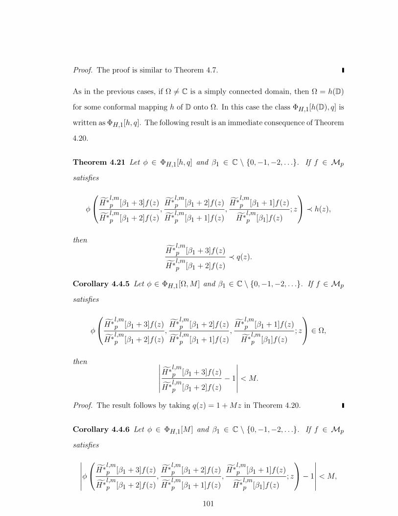
Proof. The proof is similar to Theorem 4.7.
As in the previous cases, if Ω 6= C is a simply connected domain, then Ω = h(D)
for some conformal mapping h of D onto Ω. In this case the class ΦH,1[h(D), q] is
written as ΦH,1[h, q]. The following result is an immediate consequence of Theorem
4.20.
Theorem 4.21 Let φ ∈ ΦH,1[h, q] and β1 ∈ C \ 0,−1,−2, . . .. If f ∈ Mp
satisfies
φ
H∗l,mp [β1 + 3]f(z)
H∗l,mp [β1 + 2]f(z)
,H∗
l,mp [β1 + 2]f(z)
H∗l,mp [β1 + 1]f(z)
,H∗
l,mp [β1 + 1]f(z)
H∗l,mp [β1]f(z)
; z
≺ h(z),
then
H∗l,mp [β1 + 3]f(z)
H∗l,mp [β1 + 2]f(z)
≺ q(z).
Corollary 4.4.5 Let φ ∈ ΦH,1[Ω,M ] and β1 ∈ C \ 0,−1,−2, . . .. If f ∈ Mp
satisfies
φ
H∗l,mp [β1 + 3]f(z)
H∗l,mp [β1 + 2]f(z)
,H∗
l,mp [β1 + 2]f(z)
H∗l,mp [β1 + 1]f(z)
,H∗
l,mp [β1 + 1]f(z)
H∗l,mp [β1]f(z)
; z
∈ Ω,
then ∣∣∣∣∣∣H∗l,mp [β1 + 3]f(z)
H∗l,mp [β1 + 2]f(z)
− 1
∣∣∣∣∣∣ < M.
Proof. The result follows by taking q(z) = 1 +Mz in Theorem 4.20.
Corollary 4.4.6 Let φ ∈ ΦH,1[M ] and β1 ∈ C \ 0,−1,−2, . . .. If f ∈ Mp
satisfies
∣∣∣∣∣∣φH∗l,mp [β1 + 3]f(z)
H∗l,mp [β1 + 2]f(z)
,H∗
l,mp [β1 + 2]f(z)
H∗l,mp [β1 + 1]f(z)
,H∗
l,mp [β1 + 1]f(z)
H∗l,mp [β1]f(z)
; z
− 1
∣∣∣∣∣∣ < M,
101
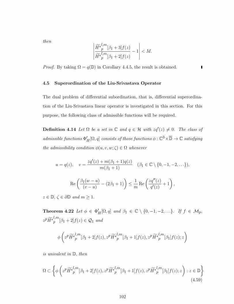
then ∣∣∣∣∣∣H∗l,mp [β1 + 3]f(z)
H∗l,mp [β1 + 2]f(z)
− 1
∣∣∣∣∣∣ < M.
Proof. By taking Ω = q(D) in Corollary 4.4.5, the result is obtained.
4.5 Superordination of the Liu-Srivastava Operator
The dual problem of differential subordination, that is, differential superordina-
tion of the Liu-Srivastava linear operator is investigated in this section. For this
purpose, the following class of admissible functions will be required.
Definition 4.14 Let Ω be a set in C and q ∈ H with zq′(z) 6= 0. The class of
admissible functions Φ′H [Ω, q] consists of those functions φ : C3×D→ C satisfying
the admissibility condition φ(u, v, w; ζ) ∈ Ω whenever
u = q(z), v =zq′(z) +m(β1 + 1)q(z)
m(β1 + 1)(β1 ∈ C \ 0,−1,−2, . . .),
Re
(β1(w − u)
(v − u)− (2β1 + 1)
)≤ 1
mRe
(zq′′(z)
q′(z)+ 1
),
z ∈ D, ζ ∈ ∂D and m ≥ 1.
Theorem 4.22 Let φ ∈ Φ′H [Ω, q] and β1 ∈ C \ 0,−1,−2, . . .. If f ∈ Mp,
zpH∗l,mp [β1 + 2]f(z) ∈ Q1 and
φ
(zpH∗
l,mp [β1 + 2]f(z), zpH∗
l,mp [β1 + 1]f(z), zpH∗
l,mp [β1]f(z); z
)
is univalent in D, then
Ω ⊂φ
(zpH∗
l,mp [β1 + 2]f(z), zpH∗
l,mp [β1 + 1]f(z), zpH∗
l,mp [β1]f(z); z
): z ∈ D
(4.59)
102
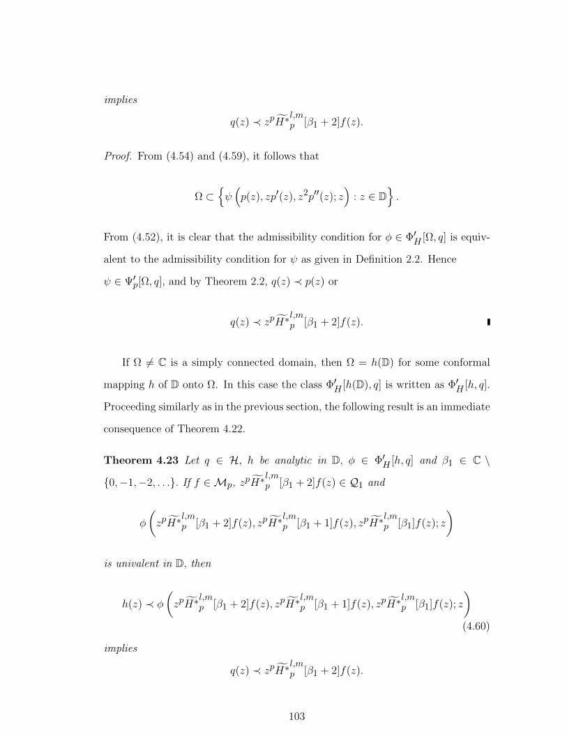
implies
q(z) ≺ zpH∗l,mp [β1 + 2]f(z).
Proof. From (4.54) and (4.59), it follows that
Ω ⊂ψ(p(z), zp′(z), z2p′′(z); z
): z ∈ D
.
From (4.52), it is clear that the admissibility condition for φ ∈ Φ′H [Ω, q] is equiv-
alent to the admissibility condition for ψ as given in Definition 2.2. Hence
ψ ∈ Ψ′p[Ω, q], and by Theorem 2.2, q(z) ≺ p(z) or
q(z) ≺ zpH∗l,mp [β1 + 2]f(z).
If Ω 6= C is a simply connected domain, then Ω = h(D) for some conformal
mapping h of D onto Ω. In this case the class Φ′H [h(D), q] is written as Φ′H [h, q].
Proceeding similarly as in the previous section, the following result is an immediate
consequence of Theorem 4.22.
Theorem 4.23 Let q ∈ H, h be analytic in D, φ ∈ Φ′H [h, q] and β1 ∈ C \
0,−1,−2, . . .. If f ∈Mp, zpH∗l,mp [β1 + 2]f(z) ∈ Q1 and
φ
(zpH∗
l,mp [β1 + 2]f(z), zpH∗
l,mp [β1 + 1]f(z), zpH∗
l,mp [β1]f(z); z
)
is univalent in D, then
h(z) ≺ φ
(zpH∗
l,mp [β1 + 2]f(z), zpH∗
l,mp [β1 + 1]f(z), zpH∗
l,mp [β1]f(z); z
)(4.60)
implies
q(z) ≺ zpH∗l,mp [β1 + 2]f(z).
103
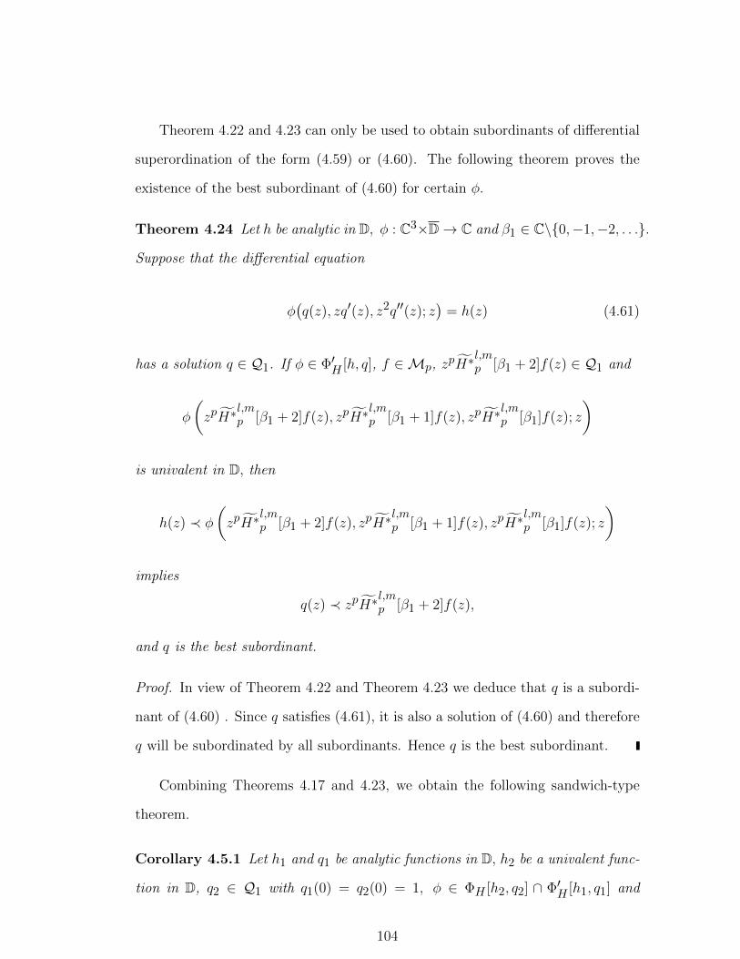
Theorem 4.22 and 4.23 can only be used to obtain subordinants of differential
superordination of the form (4.59) or (4.60). The following theorem proves the
existence of the best subordinant of (4.60) for certain φ.
Theorem 4.24 Let h be analytic in D, φ : C3×D→ C and β1 ∈ C\0,−1,−2, . . ..
Suppose that the differential equation
φ(q(z), zq′(z), z2q′′(z); z
)= h(z) (4.61)
has a solution q ∈ Q1. If φ ∈ Φ′H [h, q], f ∈Mp, zpH∗l,mp [β1 + 2]f(z) ∈ Q1 and
φ
(zpH∗
l,mp [β1 + 2]f(z), zpH∗
l,mp [β1 + 1]f(z), zpH∗
l,mp [β1]f(z); z
)
is univalent in D, then
h(z) ≺ φ
(zpH∗
l,mp [β1 + 2]f(z), zpH∗
l,mp [β1 + 1]f(z), zpH∗
l,mp [β1]f(z); z
)
implies
q(z) ≺ zpH∗l,mp [β1 + 2]f(z),
and q is the best subordinant.
Proof. In view of Theorem 4.22 and Theorem 4.23 we deduce that q is a subordi-
nant of (4.60) . Since q satisfies (4.61), it is also a solution of (4.60) and therefore
q will be subordinated by all subordinants. Hence q is the best subordinant.
Combining Theorems 4.17 and 4.23, we obtain the following sandwich-type
theorem.
Corollary 4.5.1 Let h1 and q1 be analytic functions in D, h2 be a univalent func-
tion in D, q2 ∈ Q1 with q1(0) = q2(0) = 1, φ ∈ ΦH [h2, q2] ∩ Φ′H [h1, q1] and
104
β1 ∈ C \ 0,−1,−2, . . .. If f ∈Mp, zpH∗l,mp [β1 + 2]f(z) ∈ H ∩Q1 and
φ
(zpH∗
l,mp [β1 + 2]f(z), zpH∗
l,mp [β1 + 1]f(z), zpH∗
l,mp [β1]f(z); z
)
is univalent in D, then
h1(z) ≺ φ
(zpH∗
l,mp [β1 + 2]f(z), zpH∗
l,mp [β1 + 1]f(z), zpH∗
l,mp [β1]f(z); z
)≺ h2(z)
implies
q1(z) ≺ zpH∗l,mp [β1 + 2]f(z) ≺ q2(z).
Definition 4.15 Let Ω be a set in C and q ∈ H with zq′(z) 6= 0. The class
of admissible functions Φ′H,1[Ω, q] consists of those functions φ : C3 × D → C
satisfying the admissibility condition φ(u, v, w; ζ) ∈ Ω whenever
u = q(z), v =m(β1 + 1)q(z)
m(β1 + 2)− zq′(z)−mq(z), (β1 ∈ C \ 0,−1,−2, . . .),
Re
((β + 1)u
v(β + 2)− (β + 1)u− vu
(β + 1
v− β
w− 1
)− β + 1
v− 1
)≤ 1
mRe
(zq′′(z)
q′(z)+ 1
),
z ∈ D, ζ ∈ ∂D and m ≥ 1.
Next the dual result of Theorem 4.20 for differential superordination is given.
Theorem 4.25 Let φ ∈ Φ′H,1[Ω, q] and β1 ∈ C \ 0,−1,−2, . . .. If f ∈ Mp,
H∗l,mp [β1+3]f(z)
H∗l,mp [β1+2]f(z)
∈ Q1 and
φ
H∗l,mp [β1 + 3]f(z)
H∗l,mp [β1 + 2]f(z)
,H∗
l,mp [β1 + 2]f(z)
H∗l,mp [β1 + 1]f(z)
,H∗
l,mp [β1 + 1]f(z)
H∗l,mp [β1]f(z)
; z
105
is univalent in D, then
Ω ⊂
φH∗l,mp [β1 + 3]f(z)
H∗l,mp [β1 + 2]f(z)
,H∗
l,mp [β1 + 2]f(z)
H∗l,mp [β1 + 1]f(z)
,H∗
l,mp [β1 + 1]f(z)
H∗l,mp [β1]f(z)
; z
: z ∈ D
(4.62)
implies
q(z) ≺H∗
l,mp [β1 + 3]f(z)
H∗l,mp [β1 + 2]f(z)
.
Proof. From (4.38) and (4.62), it follows that
Ω ⊂φ(p(z), zp′(z), z2p′′(z); z
): z ∈ D
.
From (4.36), the admissibility condition for φ ∈ Φ′H,2[Ω, q] is equivalent to the
admissibility condition for ψ as given in Definition 2.2. Hence ψ ∈ Ψ′[Ω, q], and
by Theorem 2.2, q(z) ≺ p(z) or
q(z) ≺H∗
l,mp [β1 + 3]f(z)
H∗l,mp [β1 + 2]f(z)
.
If Ω 6= C is a simply connected domain, then Ω = h(D) for some conformal
mapping h of D onto Ω. In this case the class Φ′H,1[h(D), q] is written as Φ′H,1[h, q].
Proceeding similarly as in the previous section, the following result is an immediate
consequence of Theorem 4.25.
Theorem 4.26 Let q ∈ H, h be analytic in D, φ ∈ Φ′H,1[h, q] and β1 ∈ C \
0,−1,−2, . . .. If f ∈Mp,H∗
l,mp [β1+3]f(z)
H∗l,mp [β1+2]f(z)
∈ Q1 and
φ
H∗l,mp [β1 + 3]f(z)
H∗l,mp [β1 + 2]f(z)
,H∗
l,mp [β1 + 2]f(z)
H∗l,mp [β1 + 1]f(z)
,H∗
l,mp [β1 + 1]f(z)
H∗l,mp [β1]f(z)
; z
106
is univalent in D, then
h(z) ≺ φ
H∗l,mp [β1 + 3]f(z)
H∗l,mp [β1 + 2]f(z)
,H∗
l,mp [β1 + 2]f(z)
H∗l,mp [β1 + 1]f(z)
,H∗
l,mp [β1 + 1]f(z)
H∗l,mp [β1]f(z)
; z
implies
q(z) ≺H∗
l,mp [β1 + 3]f(z)
H∗l,mp [β1 + 2]f(z)
.
Combining Theorems 4.21 and 4.26, the following sandwich-type theorem is
obtained.
Corollary 4.5.2 Let h1 and q1 be analytic functions in D, h2 be univalent func-
tion in D, q2 ∈ Q1 with q1(0) = q2(0) = 1, φ ∈ ΦH,1[h2, q2] ∩ Φ′H,1[h1, q1] and
β1 ∈ C \ 0,−1,−2, . . .. If f ∈Mp,H∗
l,mp [β1+3]f(z)
H∗l,mp [β1+2]f(z)
∈ H ∩Q1 and
φ
H∗l,mp [β1 + 3]f(z)
H∗l,mp [β1 + 2]f(z)
,H∗
l,mp [β1 + 2]f(z)
H∗l,mp [β1 + 1]f(z)
,H∗
l,mp [β1 + 1]f(z)
H∗l,mp [β1]f(z)
; z
is univalent in D, then
h1(z) ≺ φ
H∗l,mp [β1 + 3]f(z)
H∗l,mp [β1 + 2]f(z)
,H∗
l,mp [β1 + 2]f(z)
H∗l,mp [β1 + 1]f(z)
,H∗
l,mp [β1 + 1]f(z)
H∗l,mp [β1]f(z)
; z
≺ h2(z)
implies
q1(z) ≺H∗
l,mp [β1 + 3]f(z)
H∗l,mp [β1 + 2]f(z)
≺ q2(z).
107
CHAPTER 5
HALF-PLANE DIFFERENTIAL SUBORDINATION CHAIN
5.1 Introduction
As defined in Section 1.3.2, p. 22, Bernardi [27] introduced the linear integral
operator Fµ : A → A defined by
Fµ(z) := (µ+ 1)
∫ 1
0tµ−1f(tz)dt (µ > −1). (5.1)
It is well-known [27] that the classes of starlike, convex and close-to-convex func-
tions are closed under the Bernardi integral transform.
Parvatham considered the class R[α] of functions f ∈ A satisfying
∣∣f ′(z)− 1∣∣ < α
∣∣f ′(z) + 1∣∣ (z ∈ D, 0 < α ≤ 1),
or equivalently
f ′(z) ≺ 1 + αz
1− αz(z ∈ D, 0 < α ≤ 1),
and obtained the following result:
Theorem 5.1 [94, Theorem 2, p. 440] Let µ ≥ 0, 0 < α ≤ 1 and δ be given by
δ := α
(2− α + µ(1− α)
1 + µ(1− α)
).
If the functions f ∈ R[δ], then the function Fµ given by Bernardi’s integral (5.1)
is in R[α].
The class R[α] can be extended to the general class R[A,B] consisting of all
analytic functions f ∈ A satisfying
f ′(z) ≺ 1 + Az
1 +Bz, (z ∈ D, −1 ≤ B < A ≤ 1),
108
or the equivalent inequality
∣∣f ′(z)− 1∣∣ < ∣∣A−Bf ′(z)
∣∣ (z ∈ D, −1 ≤ B < A ≤ 1).
For 0 ≤ α < 1, the class R[1− 2α,−1] consists of functions f ∈ A for which
Re f ′(z) > α (z ∈ D, 0 < α ≤ 1),
and R[1− α, 0] is the class of functions f ∈ A satisfying the condition
∣∣f ′(z)− 1∣∣ < 1− α (z ∈ D, 0 ≤ α < 1).
When 0 < α ≤ 1, the class R[α,−α] is the class R[α] considered by Parvatham
[94].
Silverman [122], Obradovic and Tuneski [87] and many others (see [84–86,104,
105]) have studied properties of functions defined in terms of the expression
(1 +
zf ′′(z)
f ′(z)
)(f(z)
zf ′(z)
).
In fact, Silverman [122] obtained the order of starlikeness for functions in the class
Gb defined by
Gb :=
f ∈ A :
∣∣∣∣(1 +zf ′′(z)
f ′(z)
)(f(z)
zf ′(z)
)− 1
∣∣∣∣ < b, 0 < b ≤ 1, z ∈ D.
Obradovic and Tuneski [87] improved the result of Silverman [122] by showing
Gb ⊂ ST [0,−b] ⊂ ST(2/(1 +
√1 + 8b)
).
Tuneski [139] took it further and obtained conditions for the inclusion
109
Gb ⊂ ST [A,B] to hold. Letting zf ′(z)/f(z) =: p(z), the inclusion
Gb ⊂ ST [A,B] is evidently a special case of the differential chain
1 + βzp′(z)
p(z)2≺ 1 +Dz
1 + Ez⇒ p(z) ≺ 1 + Az
1 +Bz. (5.2)
For f ∈ A and 0 ≤ α < 1 Frasin and Darus [40] showed that
(zf(z))′′
f ′(z)− 2zf ′(z)
f(z)≺ (1− α)z
2− α⇒∣∣∣∣z2f ′(z)
f2(z)− 1
∣∣∣∣ < 1− α.
Letting z2f ′(z)/f2(z) as p(z), the above implication is a special case of the differ-
ential chain
1 + βzp′(z)
p(z)≺ 1 +Dz
1 + Ez⇒ p(z) ≺ 1 + Az
1 +Bz. (5.3)
Nunokawa et al. [83] showed that when p is analytic in D with p(0) = 1, then
1 + zp′(z) ≺ 1 + z ⇒ p(z) ≺ 1 + z. (5.4)
They applied this differential implication to obtain a criterion for normalized an-
alytic functions to be univalent. Clearly (5.4) is a special case of the differential
chain
1 + βzp′(z) ≺ 1 +Dz
1 + Ez⇒ p(z) ≺ 1 + Az
1 +Bz. (5.5)
The implications (5.2), (5.3) and (5.5) have been investigated in [16]. Analo-
gous results were also obtained in [8] by considering the expressions 1 + βzp′(z),
1 + β(zp′(z)/p(z)), 1 + β(zp′(z)/p2(z)) and (1 − α)p(z) + αp2(z) + βzp′(z) as
subordinate functions to the function√
1 + z that maps D onto the right-half of
the lemniscate of Bernoulli . Each led to the deduction that p is subordinated to√
1 + z.
Singh and Gupta [126] showed that whenever p and q are analytic in D with
110

p(0) = 1 = q(0) and
(1− α)p(z) + αp2(z) + αγzp′(z) ≺ (1− α)q(z) + αq2(z) + αγzq′(z),
then p(z) ≺ q(z). They also investigated similar problems in [127] and [128].
The present work investigates the differential implication
(1− α)p(z) + αp2(z) + βzp′(z) ≺ 1 + Cz
1 +Dz⇒ p(z) ≺ 1 + Az
1 +Bz. (5.6)
Using the implication (5.6), in this thesis, a more general result relating to the
Briot-Bouquet differential subordination is obtained which is then applied to the
Bernardi’s integral operator on the class R[C,D]. Analogous results are obtained
by considering the expressions p(z) + zp′(z)/p2(z) and p2(z) + zp′(z)/p(z). These
results are then used to obtain sufficient conditions for normalized analytic func-
tions in D to be Janowski starlike.
5.2 Some Subordination Results
Lemma 5.1 Let a, b, c, d ∈ R.
(i) If a 6= 0 and b2 < 3ac, then
min|t|≤1
(at3 + bt2 + ct+ d
)= b+ d− |a+ c|.
(ii) If a 6= 0 and b2 ≥ 3ac, then
min|t|≤1
(at3 + bt2 + ct+ d
)= min
(1
27a2
(2b3 − 9abc+ 27da2 − 2(b2 − 3ac)
32
), b+ d− |a+ c|
).
111

(iii) If a = 0, then
min|t|≤1
(bt2 + ct+ d
)=
4bd−c2
4b (b > 0 and |c| < 2b),
b+ d− |c| (b ≤ 0 or |c| ≥ 2b).
Proof. (i) When a 6= 0, let f(t) = at3 + bt2 + ct + d. Then f ′(t) = 3at2 + 2bt + c
and f ′′(t) = 6at+ 2b. Thus f ′(t) = 0 if
t =−b±
√b2 − 3ac
3a.
Let
t0 =−b+
√b2 − 3ac
3aand t1 =
−b−√b2 − 3ac
3a. (5.7)
If b2 < 3ac, then
min|t|≤1
(at3 + bt2 + ct+ d
)= min (f(1), f(−1))
= min a+ b+ c+ d, b+ d− (a+ c)
= b+ d− |a+ c|.
(ii) Let a 6= 0 and b2 ≥ 3ac. Using (5.7),
f ′′(t0) = f ′′(−b+
√b2 − 3ac
3a
)
= 6a
(−b+
√b2 − 3ac
3a
)+ 2b
= 2√b2 − 3ca
≥ 0
and so t0 = −b+√b2−3ac
3a gives minimum value.
112

When t1 = −b−√b2−3ac
3a ,
f ′′(−b−
√b2 − 3ac
3a
)= 6a
(−b−
√b2 − 3ac
3a
)+ 2b
= −2√b2 − 3ca
≤ 0
and so t1 = −b−√b2−3ac
3a gives maximum value. It is clear that t = t0 gives
minimum value. Also
f(t0) = f
(−b+
√(b2 − 3ac)
3a
)
=2ab3 − 9a2bc+ 27a3d− 2a(b2 − 3ac)
32
27a3
=1
27a2
(2b3 − 9abc+ 27da2 − 2(b2 − 3ac)
32
).
Thus,
min|t|<1
f(t) = min (f(t0), f(1), f(−1)) ,
or equivalently
min|t|≤1
(at3 + bt2 + ct+ d
)= min
(1
27a2
(2b3 − 9abc+ 27da2 − 2(b2 − 3ac)
32
), b+ d− |a+ c|
).
This complete the proof for part (ii).
(iii) Let a = 0. The result is clear for b = 0. Let f(t) = bt2 + ct + d. Then
f ′(t) = 2bt+ c and f ′′(t) = 2b. Thus f ′(t) = 0 if t = − c2b . For b > 0, we first note
that
f(1) = b+ d+ c, f(−1) = b+ d− c, f(− c
2b
)=−c2 + 4bd
4b
113

and
b+ d− |c| ≥ −c2 + 4bd
4b
is equivalent to
4b2 + 4bd− 4b|c| ≥ −c2 + 4bd
or
(2b− |c|)2 ≥ 0
which is trivially true. Thus, for b > 0,
f(1), f(−1) ≥ f(−c/2b).
Case(1) (b > 0, |c| < 2b)
In this case, the function f(t) attains its minimum at t = − c2b . Thus the global
minimum of f(t) is given by
min|t|≤1
f(t) = min
(f(1), f(−1), f
(− c
2b
))= f
(− c
2b
)=−c2 + 4bd
4b.
Case(2) (Otherwise)
In this case, either b < 0 or |c| ≥ 2b. If b < 0, then the point t = −c/2b gives
maximum while for |c| ≥ 2b, the point t = −c/2b lies at the boundary or outside
[-1,1]. Thus the minimum occurs only at boundary and thus the global minimum
is given by
min|t|≤1
f(t) = min(f(1), f(−1))
= min(b+ d+ c, b+ d− c)
= b+ d− |c|
114
This complete the proof for part (iii).
Now an application of Lemma 2.1 yields the following result.
Lemma 5.2 Let α, β, A and B be real numbers satisfying −1 ≤ B ≤ 0,
A 6= B, β 6= 0, and
α + β + 1
β≥∣∣∣∣(1− α− β)B + 2αA
β
∣∣∣∣ . (5.8)
Let q(z) = (1 + Az)/(1 +Bz). If p is analytic in D with p(0) = 1, and
(1− α)p(z) + αp2(z) + βzp′(z) ≺ (1− α)q(z) + αq2(z) + βzq′(z), (5.9)
then p ∈ P [A,B], and q is the best dominant.
Proof. Let the function q : D→ C be defined by
q(z) =1 + Az
1 +Bz. (5.10)
A computation from (5.10) gives
βzq′(z) =βz(A−B)
(1 +Bz)2.
Further computation shows that
(1− α)q(z) + αq2(z) + βzq′(z)
= (1− α)
(1 + Az
1 +Bz
)+ α
(1 + Az
1 +Bz
)2
+βz(A−B)
(1 +Bz)2(5.11)
=1 +
((1 + α + β)A+ (1− α− β)B
)z +
((1− α)AB + αA2
)z2
(1 +Bz)2.
115

Therefore
(1− α)q(z) + αq2(z) + βzq′(z)
=1 +
((1 + α + β)A+ (1− α− β)B
)z +
((1− α)AB + αA2
)z2
(1 +Bz)2. (5.12)
Define the function ϑ and ϕ by
ϑ(w) = (1− α)w + αw2, ϕ(w) = β
so that (5.9) becomes (2.5). Clearly the functions ϑ and ϕ are analytic in C and
ϕ(w) 6= 0. Also let Q, h : D→ C be the functions defined by
Q(z) := zq′(z)ϕ(q(z)) = βzq′(z)
and
h(z) := ϑ(q(z)) +Q(z) = (1− α)q(z) + αq2(z) + βzq′(z).
Since q is convex, the function zq′(z) is starlike, and thereforeQ is starlike univalent
in D. A computation yield
zh′(z)
Q(z)=z(1− α)q′(z)
Q(z)+
2αzq(z)q′(z)
Q(z)+zQ′(z)
Q(z)
=
α+β+1β + 1
β
((1− α− β)B + 2αA
)z
1 +Bz.
Therefore
zh′(z)
Q(z)=
a+ bz
1 +Bz
where a = α+β+1β and b = 1
β
((1− α− β)B + 2αA
).
116

In view of (5.8), it follows that
Re
(zh′(z)
Q(z)
)= Re a
(1 + b
az
1 +Bz
)≥ 0.
By Lemma 2.1, if p is analytic in D with p(0) = 1, and
(1− α)p(z) + αp2(z) + βzp′(z) ≺ (1− α)q(z) + αq2(z) + βzq′(z),
then p ∈ P [A,B], and q is the best dominant. This complete the proof.
Setting p(z) =zf ′(z)f(z)
, β = αλ and B = −1 where α, λ ∈ R, α, λ > 0 in
Lemma 5.2, we obtain the following result of Singh and Gupta [126]:
Corollary 5.2.1 [126] Let α and λ be positive real numbers. Assume that −1 <
A ≤ 1 satisfies A ≤ 1/α whenever α > 1. If f ∈ A, f(z)/z 6= 0 in D and
zf ′(z)
f(z)
(1− α + α(1− λ)
zf ′(z)
f(z)+ αλ
(1 +
zf ′′(z)
f ′(z)
))≺ h(z),
where
h(z) =1 +
((1 + α(1 + λ)
)A−
(1− α(1 + λ)
))z +
(αA2 − (1− α)A
)z2
(1− z)2,
(5.13)
then
zf ′(z)
f(z)≺ 1 + Az
1− z,
and (1 + Az)/(1− z) is the best dominant.
Remark 5.2.1 By judicious choices for A,α and λ in Corollary 5.2.1, Singh and
Gupta [126] obtained a number of known results in [61, 91,127].
The following result which is obtained by considering the expression
117

p(z) + zp′(z)/p2(z), gives sufficient condition for an analytic function to be in the
class P [A,B].
Lemma 5.3 Let −1 < B < A ≤ 1 and
A−B1− AB
≤ 1√2. (5.14)
Let q(z) = (1 + Az)/(1 +Bz). If p is analytic and p(z) 6= 0 in D, p(0) = 1 and
p(z) +zp′(z)
p2(z)≺ q(z) +
zq′(z)
q2(z), (5.15)
then p ∈ P [A,B] and q is the best dominant.
Proof. As in the proof of Lemma 5.2, let the function q be defined by
q(z) =1 + Az
1 +Bz(5.16)
and by taking the logarithmic differentiation on (5.16) gives
q(z) +zq′(z)
q2(z)=
1 + (4A−B)z + (3A2 −B2 +BA)z2 + A3z3
(1 +Bz)(1 + Az)2. (5.17)
Now to show that (5.15) implies p(z) ≺ q(z), let the functions ϑ and ϕ defined by
ϑ(w) = w, ϕ(w) =1
w2.
Since w 6= 0, the functions ϑ and ϕ are analytic in C and ϕ(w) 6= 0.
Let Q, h : D→ C be the functions defined by
Q(z) := zq′(z)ϕ(q(z)) =zq′(z)
q2(z)=z(A−B)
(1 + Az)2(5.18)
118

and
h(z) := ϑ(q(z)) +Q(z) = q(z) +zq′(z)
q2(z)=
1 + Az
1 +Bz+z(A−B)
(1 + Az)2. (5.19)
A calculation from (5.18) yields
zQ′(z)
Q(z)=
1− Az1 + Az
.
Further computations show that
Re
(zQ′(z)
Q(z)
)= Re
(1− Az1 + Az
)>|1− A|2
1− |A|2> 0 (5.20)
for −1 < A ≤ 1, which shows Q is starlike univalent in D. Now (5.18) and (5.19)
yield
zh′(z)
Q(z)= q2(z) +
zQ′(z)
Q(z).
From (5.20) it is clear that Re(zQ′(z)Q(z)
)≥ 0. Therefore, to show Re
(zh′(z)Q(z)
)> 0
it is enough to show Re(q2(z)) > 0.
q(z) =1 + Az
1 +Bz
maps the disk D onto the disk
∣∣∣∣q(z)− 1− AB1−B2
∣∣∣∣ < A−B1−B2
.
It is evident that for the disk |w − a| < r, the following inequality holds true:
| argw| ≤ sin−1(ra
).
119
Therefore,
| arg q(z)| ≤ sin−1
( A−B1−B2
1−AB1−B2
)= sin−1
(A−B1− AB
).
Further in view of (5.14), it follows that
sin−1(A−B1− AB
)≤ π
4
which implies
| arg q(z)| ≤ π
4
or
| arg q2(z)| ≤ π
2
which shows
Re(q2(z)
)> 0. (5.21)
Therefore, it is clear that from (5.20) and (5.21)
Re
(zh′(z)
Q(z)
)> 0.
By Lemma 2.1, if p is analytic and p(z) 6= 0 in D, p(0) = 1 and
p(z) +zp′(z)
p2(z)≺ q(z) +
zq′(z)
q2(z),
then p ∈ P [A,B] and q is the best dominant. This complete the proof.
Analogous to the condition in Lemma 5.3, the following result considers the ex-
pression p2(z)+zp′(z)/p(z) in order to obtain a sufficient condition for an analytic
function to be in the class P [A,B].
120
Lemma 5.4 Let −1 < B < A ≤ 1 and
A−B1− AB
≤ 1√2.
Let q(z) = (1 + Az)/(1 +Bz). If p is analytic and p(z) 6= 0 in D, p(0) = 1 and
p2(z) +zp′(z)
p(z)≺ q2(z) +
zq′(z)
q(z), (5.22)
then p ∈ P [A,B] and q is the best dominant.
Proof. Similar to the proof of Lemma 5.3, let q(z) = (1 + Az)/(1 + Bz) and by
using logarithmic differentiation on q it yields
zq′(z)
q(z)=
z(A−B)
(1 + Az)(1 +Bz).
Another computations show that,
q2(z) +zq′(z)
q(z)=
1 + (4A−B)z + (3A2 + AB −B2)z2 + A3z3
(1 + Az)(1 +Bz)2. (5.23)
Let the functions ϑ and ϕ defined by
ϑ(w) = w2, ϕ(w) =1
w.
Since w 6= 0 the functions ϑ and ϕ are analytic in C and ϕ(w) 6= 0. Analogue in
the previous theorems, let Q, h : D→ C be the functions defined by
Q(z) := zq′(z)ϕ(q(z)) =zq′(z)
q(z)(5.24)
and
h(z) := ϑ(q(z)) +Q(z) = q2(z) +zq′(z)
q(z). (5.25)
121

A computation from
Q(z) =z(A−B)
(1 + Az)(1 +Bz)
shows that
zQ′(z)
Q(z)=
1− ABz2
(1 + Az)(1 +Bz). (5.26)
Thus
Re
(1− ABz2
(1 + Az)(1 +Bz)
)= Re
(1
1 + Az+
1
1 +Bz− 1
)>
1
1 + |A|+
1
1 + |B|− 1
=1− |AB|
(1 + |A|)(1 + |B|)> 0 (−1 < B < A ≤ 1).
Therefore
Re
(zQ′(z)
Q(z)
)> 0. (5.27)
Therefore Q is starlike univalent in D. Now (5.24) and (5.25) yield
h(z) = q2(z) +Q(z) = 2q2(z) +zQ′(z)
Q(z).
From the proof of Theorem 5.3, it is clear that Re(q2(z)) > 0 and (5.27) show that
Re(zQ′(z)Q(z)
)≥ 0. Therefore, Re
(zh′(z)Q(z)
)> 0. By Lemma 2.1, it is proven that, if
p is analytic and p(z) 6= 0 in D, p(0) = 1 and
p2(z) +zp′(z)
p(z)≺ q2(z) +
zq′(z)
q(z),
then p ∈ P [A,B] and q is the best dominant. This complete the proof.
5.3 Sufficient Conditions for Starlikeness
By making use of Lemma 5.1(iii) and Lemma 5.2, the following result is proved.
122

Theorem 5.2 Let A, B, C, D, α and β be real numbers satisfying |D| ≤ 1, C 6=
D, |B| ≤ 1, A 6= B and β 6= 0. Let b = −4KM, c = 2(IJ − L(K + M)
)and
d = I2 + J2 − L2 − (M −K)2, where I = (A−B)(1 + α + β),
J = (A−B)(Aα+B), K = C −D, L = 2CB−DA(1 +α+ β)−DB(1−α− β)
and M = CB2 −DA(B + α(A−B)
). Let
α + β + 1
β≥∣∣∣∣(1− α− β)B + 2αA
β
∣∣∣∣ .Further, suppose one of the following conditions hold:
(i) If b > 0 and |c| < 2b, then c2 ≤ 4bd,
(ii) If b ≤ 0 or |c| ≥ 2b, then |c| ≤ b+ d.
If an analytic function p in D satisfies p(0) = 1 and the subordination
(1− α)p(z) + αp2(z) + βzp′(z) ≺ 1 + Cz
1 +Dz,
then p ∈ P [A,B].
Proof. Let q be the convex function given by q(z) = (1 + Az)/(1 + Bz). By
Lemma 5.2, it follows that the subordination
(1− α)p(z) + αp2(z) + βzp′(z) ≺ (1− α)q(z) + αq2(z) + βzq′(z)
implies
p(z) ≺ q(z).
The result is proved if it could be shown that
g(z) :=1 + Cz
1 +Dz≺ (1− α)q(z) + αq2(z) + βzq′(z) =: h(z) (5.28)
123
Since g is univalent, the subordination g(z) ≺ h(z) is equivalent to the subordina-
tion
z ≺ g−1(h(z)) =: H(z).
The proof will be completed by showing that |H(eiθ)| ≥ 1 for all θ ∈ [0, 2π]. First
note that from (5.12) we have
h(z) =(1− α)(1 + Az)(1 +Bz) + α(1 + Az)2 + βz(A−B)
(1 +Bz)2. (5.29)
Furthermore
q(z) =1 + Cz
1 +Dz
yields
g−1(w) =w − 1
C −Dw. (5.30)
Replacing w = h(z) in g−1(w), we obtain
H(z) = g−1(h(z))
=h(z)− 1
C −Dh(z)
=(A−B)(1 + α + β)z + (A−B)(Aα +B)z2
C −D +(2CB −DA(1 + α + β)−DB(1− α− β)
)z
+(CB2 −DA
(B + α(A−B)
))z2
By writing,
I = (A−B)(1 + α + β),
J = (A−B)(Aα +B),
K = C −D,
L = 2CB −DA(1 + α + β)−DB(1− α− β),
124
and
M = CB2 −DA(B + α(A−B)
)we see that
H(z) = g−1(h(z)) =Iz + Jz2
K + Lz +Mz2
=z(I + Jz)
z(Kz−1 + L+Mz)
=I + Jz
Kz−1 + L+Mz.
Replacing z = eiθ in |H(z)| we get
|H(eiθ)| =
∣∣∣∣∣ I + Jeiθ
Ke−iθ + L+Meiθ
∣∣∣∣∣
=
∣∣∣∣ I + J cos θ + iJ sin θ
K cos θ − iK sin θ + L+M cos θ + iM sin θ
∣∣∣∣
=
∣∣∣∣ I + J cos θ + iJ sin θ
L+ (K +M) cos θ + i(M −K) sin θ
∣∣∣∣ .Further computations show that,
|H(eiθ)|2 ≥ 1
or
(I + J cos θ)2 + J2 sin2 θ(L+ (K +M) cos θ
)2+ (M −K)2 sin2 θ
≥ 1
or
I2 + 2IJ cos θ + J2 cos2 θ + J2(1− cos2 θ)
L2 + 2L(K +M) cos θ + (K +M)2 cos2 θ + (M −K)2(1− cos2 θ)≥ 1
125
or
I2 + J2 − L2 − (M −K)2 + 2(IJ − L(K +M)
)cos θ − 4KM cos2 θ ≥ 0. (5.31)
Let
b = −4KM,
c = 2(IJ − L(K +M)
),
d = I2 + J2 − L2 − (M −K)2,
and
t = cos θ.
Then (5.31) can be written as,
bt2 + ct+ d ≥ 0.
Now |H(eiθ)|2 ≥ 1 provided bt2 + ct+ d ≥ 0 or equivalently
min|t|≤1
(bt2 + ct+ d
)≥ 0.
By using Lemma 5.1(iii), we see that
min|t|≤1
(bt2 + ct+ d
)=
4bd−c2
4b (b > 0 and |c| < 2b),
b+ d− |c| (b ≤ 0 or |c| ≥ 2b).
Therefore, |H(eiθ)| ≥ 1 provided that when b > 0 and |c| < 2b
4bd− c2
4b≥ 0
126

or equivalently c2 ≤ 4bd , or when b ≤ 0 or |c| ≥ 2b
|c| ≤ b+ d.
This complete the proof.
An application of Theorem 5.2 to the Bernardi’s integral operator on the class
R[C,D] yields the following result.
Theorem 5.3 [17, Theorem 3.2] Let the conditions of Theorem 5.2 hold with
α = 0 and β = 1/(µ+ 1). If f ∈ R[C,D], then Fµ given by the Bernardi’s integral
(5.1) is in R[A,B].
Proof. It follows from (5.1) that
(µ+ 1)f(z) = zF ′µ(z) + µFµ(z),
and so
f ′(z) = F ′µ(z) +zF ′′µ (z)
µ+ 1.
The result now follows from Theorem 5.2 with p(z) = F ′µ(z), α = 0 and
β = 1/(µ+ 1).
For A = γ, B = −γ, C = δ and D = −δ (0 < γ, δ ≤ 1),
then I = 2γ((µ+2)/(µ+1)
), J = −2γ2, K = 2δ, L = −2µδγ/(µ+1) and M = 0.
Since KM = 0, condition (ii) in Theorem 5.2 holds provided
2γ(µ+ 1)∣∣∣γ2(µ+ 2) + δ2µ
∣∣∣ ≤ γ2(µ2(1− δ2) + 4(µ+ 1)
)+ (γ4 − δ2)(µ+ 1)2.
Thus, Theorem 5.3 yields the following result (see also [17, Remark 3.3]):
127
Corollary 5.3.1 Let µ > −1, 0 < γ, δ ≤ 1 and
2γ(µ+ 1)∣∣∣γ2(µ+ 2) + δ2µ
∣∣∣ ≤ γ2(µ2(1− δ2) + 4(µ+ 1)
)+ (γ4 − δ2)(µ+ 1)2.
If f ∈ R[δ], then Fµ given by the Bernardi’s integral (5.1) lies in R[γ].
Note that Corollary 5.3.1 extends Theorem 5.1 from the case µ ≥ 0 to µ > −1.
For A = 1− γ, B = 0, C = 1− δ and D = 0 (0 < γ, δ ≤ 1), then
I = (1−γ)((µ+2)/(µ+1)
), J = 0, K = 1− δ, L = 0 and M = 0. Since KM = 0,
condition (ii) in Theorem 5.2 holds provided (1 − δ)/(1 − γ) ≤ (µ + 2)/(µ + 1).
Thus, Theorem 5.3 yields the following result (also see [17, Corollary 3.3]):
Corollary 5.3.2 Let µ > −1, 0 < γ, δ ≤ 1 and
1− δ1− γ
≤ µ+ 2
µ+ 1.
If f ∈ Rδ, then Fµ given by Bernardi’s integral (5.1) is in Rγ .
An application of Theorem 5.2 yield the sufficient conditions for normalized ana-
lytic function to be Janowski starlike.
Theorem 5.4 Let the conditions of Theorem 5.2 holds. If f ∈ A satisfies
zf ′(z)
f(z)
(β
(1 +
zf ′′(z)
f ′(z)− zf ′(z)
f(z)
)+ α
zf ′(z)
f(z)+ (1− α)
)≺ 1 + Cz
1 +Dz
then f ∈ ST [A,B].
Proof. With p(z) =zf ′(z)f(z)
, a computation shows that
(1− α)p(z) + αp2(z) + βzp′(z)
= (1− α)zf ′(z)
f(z)+ α
(zf ′(z)
f(z)
)2
+ βzf ′(z)
f(z)
(1 +
zf ′′(z)
f ′(z)− zf ′(z)
f(z)
)128
=zf ′(z)
f(z)
(β
(1 +
zf ′′(z)
f ′(z)− zf ′(z)
f(z)
)+ α
zf ′(z)
f(z)+ (1− α)
).
The result now follows from Theorem 5.2.
The following sufficient condition for starlikeness of order γ is an application
of Theorem 5.4.
Corollary 5.3.3 If f ∈ A satisfies
∣∣∣∣zf ′(z)
f(z)
(1 +
zf ′′(z)
f ′(z)− zf ′(z)
f(z)
)− 1
∣∣∣∣ < 1− γ2
(0 ≤ γ < 1),
then f ∈ ST (γ)
Proof. The result follows from Theorem 5.4 by taking α = 0, β = 1,
A = 1− 2γ, B = −1, C = (1− γ)/2 and D = 0 (0 ≤ γ < 1).
An application of Lemma 5.1 and Lemma 5.3 gives the following result.
Theorem 5.5 Let −1 < B < A ≤ 1, −1 ≤ D < C ≤ 1 and (A − B)/(1 −
AB) ≤ 1/√
2. Let a = −8LR, b = 4IK − 4(LN + RM), c = 2J(I + K) −
2(NM +LM +NR− 3LR) and d = J2 + (K− I)2− (M −R)2− (L−N)2, where
I = 2(A − B), J = (2A + B)(A − B), K = A2(A − B), L = (C − D), M =(C(2A + B) − D(4A − B)
), N =
(AC(A + 2B) − D(3A2 + AB − B2)
), and
R = A2(BC −DA). Further, suppose one of the following conditions hold:
(1) Let a 6= 0.
(i) If
b2 ≥ 3ac and |a+c| < b+d− 1
27a2
(2b3 − 9abc+ 27da2 − 2(b2 − 3ac)
32
),
then
2b3 − 9abc+ 27da2 − 2(b2 − 3ac)32 ≥ 0,
129
(ii) If
b2 < 3ac or |a+c| ≥ b+d− 1
27a2
(2b3 − 9abc+ 27da2 − 2(b2 − 3ac)
32
),
then
|a+ c| ≤ b+ d.
(2) Let a = 0.
(i) If b > 0 and |c| < 2b, then c2 ≤ 4bd,
(ii) If b ≤ 0 or |c| ≥ 2b, then |c| ≤ b+ d.
If p is analytic and p(z) 6= 0 in D, p(0) = 1 and satisfies the subordination
p(z) +zp′(z)
p2(z)≺ 1 + Cz
1 +Dz,
then p ∈ P [A,B].
Proof. Let the function q be defined by q(z) = (1 + Az)/(1 + Bz). Similar to the
proof of Theorem 5.2, by Lemma 5.3 it follows that the subordination
p(z) +zp′(z)
p2(z)≺ q(z) +
zq′(z)
q2(z)
implies p(z) ≺ q(z). In light of differential chain, the result is proved if it could be
shown that
g(z) :=1 + Cz
1 +Dz≺ q(z) +
zq′(z)
q2(z)=: h(z). (5.32)
Since g is univalent, the subordination g(z) ≺ h(z) is equivalent to the subordina-
tion
z ≺ g−1(h(z)) =: H(z).
The proof will be completed by showing that |H(eiθ)| ≥ 1 for all θ ∈ [0, 2π]. First
130

note that from (5.17) we have
h(z) =1 + (4A−B)z + (3A2 −B2 +BA)z2 + A3z3
(1 +Bz)(1 + Az)2. (5.33)
Now (5.33) and (5.30) yield
H(z) = g−1(h(z))
=h(z)− 1
C −Dh(z)
=2(A−B)z + (2A+B)(A−B)z2 + A2(A−B)z3
C −D +((C(2A+B)−D(4A−B)
)z
+(AC(A+ 2B)−D(3A2 + AB −B2)
)z2 + A2(BC −DA)z3
.
By writing,
I = 2(A−B),
J = (2A+B)(A−B),
K = A2(A−B),
L = C −D,
M =(C(2A+B)−D(4A−B)
),
N =(AC(A+ 2B)−D(3A2 + AB −B2)
),
and
R = A2(BC −DA)
we see that
H(z) =Iz + Jz2 +Kz3
L+Mz +Nz2 +Rz3(5.34)
=z(Iz−1 + J +Kz
)Lz−1 +M +Nz +Rz2
.
131
Replacing z = eiθ in |H(z)| we get
|H(eiθ)| =
∣∣∣∣∣∣eiθ(Ie−iθ + J +Keiθ
)Le−iθ +M +Neiθ +Rei2θ
∣∣∣∣∣∣
=
∣∣∣∣ J + (I +K) cos θ + i(K − I) sin θ
M + (L+N) cos θ +R cos 2θ + i[(N − L) sin θ +R sin 2θ]
∣∣∣∣ .A computation shows that,
|H(eiθ)|2 ≥ 1
or
(J + (I +K) cos θ
)2+ (K − I)2 sin2 θ(
M + (L+N) cos θ +R cos 2θ)2
+((N − L) sin θ +R sin 2θ
)2 ≥ 1 (5.35)
From the numerator of (5.35), computations show that
(J + (I +K) cos θ
)2+ (K − I)2 sin2 θ
= J2 + (K − I)2 + 2J(I +K) cos θ + 4IK cos2 θ.
Similarly, from the denominator of (5.35), computations show that
(M + (L+N) cos θ +R cos 2θ
)2= (M −R)2 + 2(M −R)(L+N) cos θ +
((L+N)2 + 4R(M −R)
)cos2 θ
+ 4R(L+N) cos3 θ + 4R2 cos4 θ,
and((N − L) sin θ +R sin 2θ
)2= (L−N)2 − 4R(L−N) cos θ +
(4R2 − (L−N)2
)cos2 θ
+ 4R(L−N) cos3 θ − 4R2 cos4 θ.
132

Therefore
(M + (L+N) cos θ +R cos 2θ)2 + ((N − L) sin θ +R sin 2θ)2
= (M −R)2 + (L−N)2 + 2(NM + LM +NR− 3LR) cos θ
+ 4(LN +RM) cos2 θ + 8LR cos3 θ.
Now (5.35) can be written as
J2 + (K − I)2 + 2J(I +K) cos θ + 4IK cos2 θ
(M −R)2 + (L−N)2 + 2(NM + LM +NR− 3LR) cos θ
+4(LN +RM) cos2 θ + 8LR cos3 θ
≥ 1,
or equivalently
J2 + (K − I)2 − (M −R)2 − (L−N)2
+(2J(I +K)− 2(NM + LM +NR− 3LR)
)cos θ
+(4IK − 4(LN +RM)
)cos2 θ − 8LR cos3 θ ≥ 0. (5.36)
Let
a = −8LR,
b = 4IK − 4(LN +RM),
c = 2J(I +K)− 2(NM + LM +NR− 3LR),
d = J2 + (K − I)2 − (M −R)2 − (L−N)2,
and
t = cos θ.
Then (5.36) becomes,
at3 + bt2 + ct+ d ≥ 0.
133

To show that |H(eiθ)|2 ≥ 1 we have to prove at3 + bt2 + ct+ d ≥ 0 or equivalently
min|t|≤1
(at3 + bt2 + ct+ d
)≥ 0.
Thus, in view of Lemma 5.1 |H(eiθ)| ≥ 1 if one of the following condition holds:
(1) Let a 6= 0.
(i) If
b2 ≥ 3ac and1
27a2
(2b3 − 9abc+ 27da2 − 2(b2 − 3ac)
32
)< b+d−|a+c|,
then
min|t|≤1
(at3 + bt2 + ct+ d
)=
1
27a2
(2b3 − 9abc+ 27da2 − 2(b2 − 3ac)
32
)≥ 0
which implies
2b3 − 9abc+ 27da2 − 2(b2 − 3ac)32 ≥ 0.
(ii) If
b2 < 3ac or1
27a2
(2b3 − 9abc+ 27da2 − 2(b2 − 3ac)
32
)≥ b+d−|a+c|,
then
min|t|≤1
(at3 + bt2 + ct+ d
)= b+ d− |a+ c| ≥ 0
which implies
|a+ c| ≤ b+ d.
134

(2) Let a = 0.
(i) If b > 0 and |c| < 2b, then
min|t|≤1
(bt2 + ct+ d
)=
4bd− c2
4b≥ 0
which implies c2 ≤ 4bd,
(ii) If b ≤ 0 or |c| ≥ 2b, then
min|t|≤1
(bt2 + ct+ d
)= b+ d− |c| ≥ 0
which implies |c| ≤ b+ d.
This complete the proof.
The following theorem which gives sufficient condition for Janowski starlikeness is
a consequence of Theorem 5.5.
Theorem 5.6 Let the conditions of Theorem 5.5 holds. If f ∈ A satisfies
f(z)
zf ′(z)
(1 +
zf ′′(z)
f ′(z)
)+zf ′(z)
f(z)− 1 ≺ 1 + Cz
1 +Dz
then f ∈ ST [A,B].
Proof. With p(z) =zf ′(z)f(z)
, logarithmic differentiation yields
p(z) +zp′(z)
p2(z)=
f(z)
zf ′(z)
(1 +
zf ′′(z)
f ′(z)
)+zf ′(z)
f(z)− 1.
The result now follows from Theorem 5.5.
Lemma 5.1 and Lemma 5.4 will be use to prove the following result.
135

Theorem 5.7 Let −1 < B < A ≤ 1, −1 ≤ D < C ≤ 1 and (A − B)/(1 −
AB) ≤ 1/√
2. Let a = −8LR, b = 4IK − 4(LN + RM), c = 2J(I + K) −
2(NM +LM +NR− 3LR) and d = J2 + (K− I)2− (M −R)2− (L−N)2, where
I = 3(A − B), J = (3A + 2B)(A − B), K = A(A2 − B2), L = (C − D), M =(C(A + 2B) − D(4A − B)
), N =
(BC(2A + B) − D(3A2 + AB − B2)
), and
R = A(CB2 −DA2). Further, suppose one of the following conditions hold:
(1) Let a 6= 0.
(i) If
b2 ≥ 3ac and |a+c| < b+d− 1
27a2
(2b3 − 9abc+ 27da2 − 2(b2 − 3ac)
32
),
then
2b3 − 9abc+ 27da2 − 2(b2 − 3ac)32 ≥ 0,
(ii) If
b2 < 3ac or |a+c| ≥ b+d− 1
27a2
(2b3 − 9abc+ 27da2 − 2(b2 − 3ac)
32
),
then
|a+ c| ≤ b+ d.
(2) Let a = 0.
(i) If b > 0 and |c| < 2b, then c2 ≤ 4bd,
(ii) If b ≤ 0 or |c| ≥ 2b, then |c| ≤ b+ d.
If p is analytic and p(z) 6= 0 in D, p(0) = 1 and satisfies the subordination
p2(z) +zp′(z)
p(z)≺ 1 + Cz
1 +Dz,
136

then p ∈ P [A,B].
Proof. Defined q(z) = (1 + Az)/(1 + Bz). Analogue to the proof of Theorem 5.5,
it is sufficient to prove
g(z) :=1 + Cz
1 +Dz≺ q2(z) +
zq′(z)
q(z)=: h(z)
or equivalently by noting that
g(z) ≺ h(z)⇒ z ≺ g−1(h(z)) =: H(z)
we show that |H(eiθ)| ≥ 1 for all θ ∈ [0, 2π]. From (5.23) we have
h(z) =1 + (4A−B)z + (3A2 −B2 +BA)z2 + A3z3
(1 + Az)(1 +Bz)2. (5.37)
Now (5.37) and (5.30) yield
H(z) = g−1(h(z))
=h(z)− 1
C −Dh(z)
=3(A−B)z + (3A+ 2B)(A−B)z2 + A(A2 −B2)z3
C −D +(C(A+ 2B)−D(4A−B)
)z
+(BC(2A+B)−D(3A2 + AB −B2)
)z2 + A(CB2 −DA2)z3
.
By writing,
I = 3(A−B),
J = (3A+ 2B)(A−B),
K = A(A2 −B2),
L = (C −D),
137

M =(C(A+ 2B)−D(4A−B)
),
N =(BC(2A+B)−D(3A2 + AB −B2)
),
and
R = A(CB2 −DA2)
we see that
H(z) = g−1(h(z)) =Iz + Jz2 +Kz3
L+Mz +Nz2 +Rz3.
The proof of the remaining parts run along similar lines with the proof of Theo-
rem 5.5, p. 131. Therefore it is omitted.
Theorem 5.8 Let the conditions of Theorem 5.7 holds. If f ∈ A satisfies
1 +zf ′′(z)
f ′(z)+zf ′(z)
f(z)
(zf ′(z)
f(z)− 1
)≺ 1 + Cz
1 +Dz
then f ∈ ST [A,B].
Proof. With p(z) =zf ′(z)f(z)
, a computation shows that
p2(z) +zp′(z)
p(z)= 1 +
zf ′′(z)
f ′(z)+zf ′(z)
f(z)
(zf ′(z)
f(z)− 1
).
The result now follows from Theorem 5.8.
138

CHAPTER 6
HARMONIC FUNCTIONS ASSOCIATED WITH
HYPERGEOMETRIC FUNCTIONS
6.1 Introduction
In the well-established theory of analytic univalent functions, there are several
studies on hypergeometric functions associated with classes of analytic functions
(See for example [30, 36, 59, 71, 89, 98, 117, 124, 136, 137]) investigating univalence,
starlikeness and other properties of these functions. On the other hand only some
corresponding studies on connections of hypergeometric functions with harmonic
mappings have been done [5,6,22,77]. Pursuing this line of study, results that bring
out connections of hypergeometric functions with a class of harmonic univalent
functions considered in [145] are investigated in this chapter.
Recall that, for f = h+ g ∈ SH the series expansion for the analytic functions
h and g are expressed as
h(z) = z +∞∑n=2
anzn and g(z) =
∞∑n=1
bnzn, |b1| < 1. (6.1)
If φ1 and φ2 are analytic and f = h+ g is in SH , the convolution or the Hadamard
product is defined by
f ∗ (φ1 + φ2) = h ∗ φ1 + g ∗ φ2.
Let a, b and c be any complex numbers with c 6= 0,−1,−2,−3, · · · . As defined in
Subsection 1.3.2, p. 23, the Gaussian hypergeometric function is defined by
F (a, b; c; z) =∞∑n=0
(a)n(b)n(c)n(1)n
zn, (6.2)
where (λ)n is the Pochhammer symbol defined by (1.19).
139

Since the hypergeometric series in (6.2) converges absolutely in D, it follows
that F (a, b; c; z) defines a function which is analytic in D, provided that c is neither
zero nor a negative integer. In fact, F (a, b; c; 1) converges for Re(c − a − b > 0)
and is related to the gamma given by
F (a, b; c; 1) =Γ(c)Γ(c− a− b)Γ(c− a)Γ(c− b)
, c 6= 0, 1, 2, . . . (6.3)
In particular, the incomplete beta function, related to the Gaussian hyperge-
ometric function ϕ(a, c; z), is defined by
ϕ(a, c; z) = zF (a, 1; c; z) =∞∑n=0
(a)n(c)n
zn+1, z ∈ U , c 6= 0, 1, 2, . . . . (6.4)
Throughout this thesis, let G(z) = φ1(z) + φ2(z) be a function where φ1(z)
and φ2(z) are the hypergeometric functions defined by
φ1(z) := zF (a1, b1; c1; z) = z +∞∑n=2
(a1)n−1(b1)n−1
(c1)n−1(1)n−1zn, (6.5)
φ2(z) := F (a2, b2; c2 : z)− 1 =∞∑n=1
(a2)n(b2)n(c2)n(1)n
zn, |a2b2| < |c2|. (6.6)
Based on the study in [145], for α ≥ 0 and 0 ≤ β < 1, let HP (α, β) denote
the class of harmonic functions of the form (6.1) satisfying the condition
Re(αz(h′′(z) + g′′(z)
)+(h′(z) + g′(z)
))> β.
Also denote by HT (α, β) = HP (α, β)⋂TH where TH [123], is the class of
harmonic functions f such that
f(z) = z −∞∑n=2
|an|zn −∞∑n=1
|bn|zn, |b1| < 1. (6.7)
140
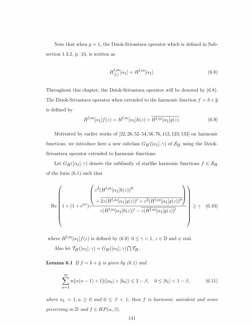
Note that when p = 1, the Dziok-Srivastava operator which is defined in Sub-
section 1.3.2, p. 24, is written as
Hl,m(1)
[α1] = H l,m[α1]. (6.8)
Throughout this chapter, the Dziok-Srivastava operator will be denoted by (6.8).
The Dziok-Srivastava operator when extended to the harmonic function f = h+ g
is defined by
H l,m[α1]f(z) = H l,m[α1]h(z) +H l,m[α1]g(z). (6.9)
Motivated by earlier works of [22, 26, 52–54, 56, 76, 112, 123, 133] on harmonic
functions, we introduce here a new subclass GH([α1], γ) of SH using the Dziok-
Srivastava operator extended to harmonic functions.
Let GH([α1], γ) denote the subfamily of starlike harmonic functions f ∈ SH
of the form (6.1) such that
Re
1 + (1 + eiψ)
z2(H l,m[α1]h(z))′′
+ 2z(H l,m[α1]g(z))′ + z2(H l,m[α1]g(z))′′
z(H l,m[α1]h(z))′ − z(H l,m[α1]g(z))′
≥ γ (6.10)
where H l,m[α1]f(z) is defined by (6.9) 0 ≤ γ < 1, z ∈ D and ψ real.
Also let TH([α1], γ) = GH([α1], γ)⋂TH .
Lemma 6.1 If f = h+ g is given by (6.1) and
∞∑n=1
n(α(n− 1) + 1
)(|an|+ |bn|) ≤ 2− β, 0 ≤ |b1| < 1− β, (6.11)
where a1 = 1, α ≥ 0 and 0 ≤ β < 1, then f is harmonic univalent and sense
preserving in D and f ∈ HP (α, β).
141

Proof. For |z1| ≤ |z2| < 1, we have
|f(z1)− f(z2)| ≥ |h(z1)− h(z2)| − |g(z1)− g(z2)|
=
∣∣∣∣∣(z1 − z2) +∞∑n=2
an(zn1 − zn2 )
∣∣∣∣∣−∣∣∣∣∣∞∑n=1
bn(zn1 − zn2 )
∣∣∣∣∣≥ |z1 − z2| −
∞∑n=2
|an||zn1 − zn2 | −
∞∑n=1
|bn||zn1 − zn2 |
= |z1 − z2|
(1− |b1| −
∞∑n=2
(|an|+ |bn|)∣∣∣∣zn1 − zn2z1 − z2
∣∣∣∣)
≥ |z1 − z2|
(1− |b1| −
∞∑n=2
n(|an|+ |bn|)|z2|n−1
)
≥ |z1 − z2|
(1− |b1| − |z2|
∞∑n=2
n(α(n− 1) + 1)(|an|+ |bn|)
)
≥ |z1 − z2| (1− β − |b1| − |z2|(1− β − |b1|))
= |z1 − z2|(1− β − |b1|)(1− |z2|) > 0.
Hence, |f(z1)− f(z2)| > 0 and f is univalent in D. To prove f is locally univalent
and sense-preserving in D, it is enough to show that |h′(z)| > |g′(z)|.
|h′(z)| ≥ 1−∞∑n=2
n|an||z|n−1
> 1−∞∑n=2
n|an|
≥ 1− β −∞∑n=2
n(α(n− 1) + 1)|an|
≥∞∑n=1
n(α(n− 1) + 1)|bn|
>
∞∑n=1
n|bn||z|n−1 = |g′(z)|.
Using the fact that Rew > β if and only if |1−β+w| > |1 +β−w|, it is sufficient
142

to show that
|1−β+αz(h′′(z)+g′′(z))+h′(z)+g′(z)|−|1+β−αz(h′′(z)+g′′(z))−h′(z)−g′(z)| > 0
(6.12)
in proving f ∈ HP (α, β). Substituting for h(z) and g(z) in (6.12) yields,
∣∣∣∣∣2− β +∞∑n=2
n(α(n− 1) + 1)anzn−1 +
∞∑n=1
n(α(n− 1) + 1)bnzn−1
∣∣∣∣∣−
∣∣∣∣∣β −∞∑n=2
n(α(n− 1) + 1)anzn−1 −
∞∑n=1
n(α(n− 1) + 1)bnzn−1
∣∣∣∣∣≥ (2− β)−
∞∑n=2
n(α(n− 1) + 1)|an||z|n−1 −∞∑n=1
n(α(n− 1) + 1)|bn||z|n−1
− β −∞∑n=2
n(α(n− 1) + 1)|an||z|n−1 −∞∑n=1
n(α(n− 1) + 1)|bn||z|n−1
≥ 2
(1− β − |z|
( ∞∑n=2
n(α(n− 1) + 1)|an|+∞∑n=1
n(α(n− 1) + 1)|bn|
))
≥ 2(1− β)(1− |z|) > 0
by the condition (6.11).
6.2 Coefficient Condition for Gaussian Hypergeometric Function
Theorem 6.1 If aj , bj > 0 and cj > aj + bj + 2 for j = 1, 2, then a sufficient
condition for G = φ1 + φ2 to be harmonic univalent in D and G ∈ HP (α, β), is
that
(α(a1)2(b1)2
(c1 − a1 − b1 − 2)2+
a1b1(2α + 1)
c1 − a1 − b1 − 1+ 1
)F (a1, b1; c1; 1) (6.13)
+
(α(a2)2(b2)2
(c2 − a2 − b2 − 2)2+
a2b2c2 − a2 − b2 − 1
)F (a2, b2; c2; 1) ≤ 2− β
143

where α ≥ 0 and 0 ≤ β < 1.
Proof. Let
G(z) = φ1(z) + φ2(z)
= z +∞∑n=2
(a1)n−1(b1)n−1
(c1)n−1(1)n−1zn +
∞∑n=1
(a2)n(b2)n(c2)n(1)n
zn.
When the condition (6.13) holds for the coefficients of G = φ1 + φ2, it is enough
to prove that
∞∑n=1
n(α(n− 1) + 1)
((a1)n−1(b1)n−1
(c1)n−1(1)n−1+
(a2)n(b2)n(c2)n(1)n
)≤ 2− β. (6.14)
Write the left side of equality (6.14) as
α∞∑n=1
n(n− 1)(a1)n−1(b1)n−1
(c1)n−1(1)n−1+ α
∞∑n=1
n(n− 1)(a2)n(b2)n(c2)n(1)n
+∞∑n=1
n(a1)n−1(b1)n−1
(c1)n−1(1)n−1+∞∑n=1
n(a2)n(b2)n(c2)n(1)n
= α∞∑n=1
[(n− 1)2 + (n− 1)](a1)n−1(b1)n−1
(c1)n−1(1)n−1+ α
∞∑n=1
(n2 − n)(a2)n(b2)n(c2)n(1)n
+∞∑n=1
(n− 1 + 1)(a1)n−1(b1)n−1
(c1)n−1(1)n−1+∞∑n=1
n(a2)n(b2)n(c2)n(1)n
= α
∞∑n=1
n2 (a1)n(b1)n(c1)n(1)n
+ (α + 1)∞∑n=1
n(a1)n(b1)n(c1)n(1)n
+∞∑n=0
(a1)n(b1)n(c1)n(1)n
+ α∞∑n=1
n2 (a2)n(b2)n(c2)n(1)n
− (α− 1)∞∑n=1
n(a2)n(b2)n(c2)n(1)n
= α
((a1)2(b1)2
(c1 − a1 − b1 − 2)2+
a1b1c1 − a1 − b1 − 1
)F (a1, b1; c1; 1)
+(α + 1)a1b1F (a1, b1; c1; 1)
c1 − a1 − b1 − 1+ F (a1, b1; c1; 1)
+ α
((a2)2(b2)2
(c2 − a2 − b2 − 2)2+
a2b2c2 − a2 − b2 − 1
)F (a2, b2; c2; 1)
144
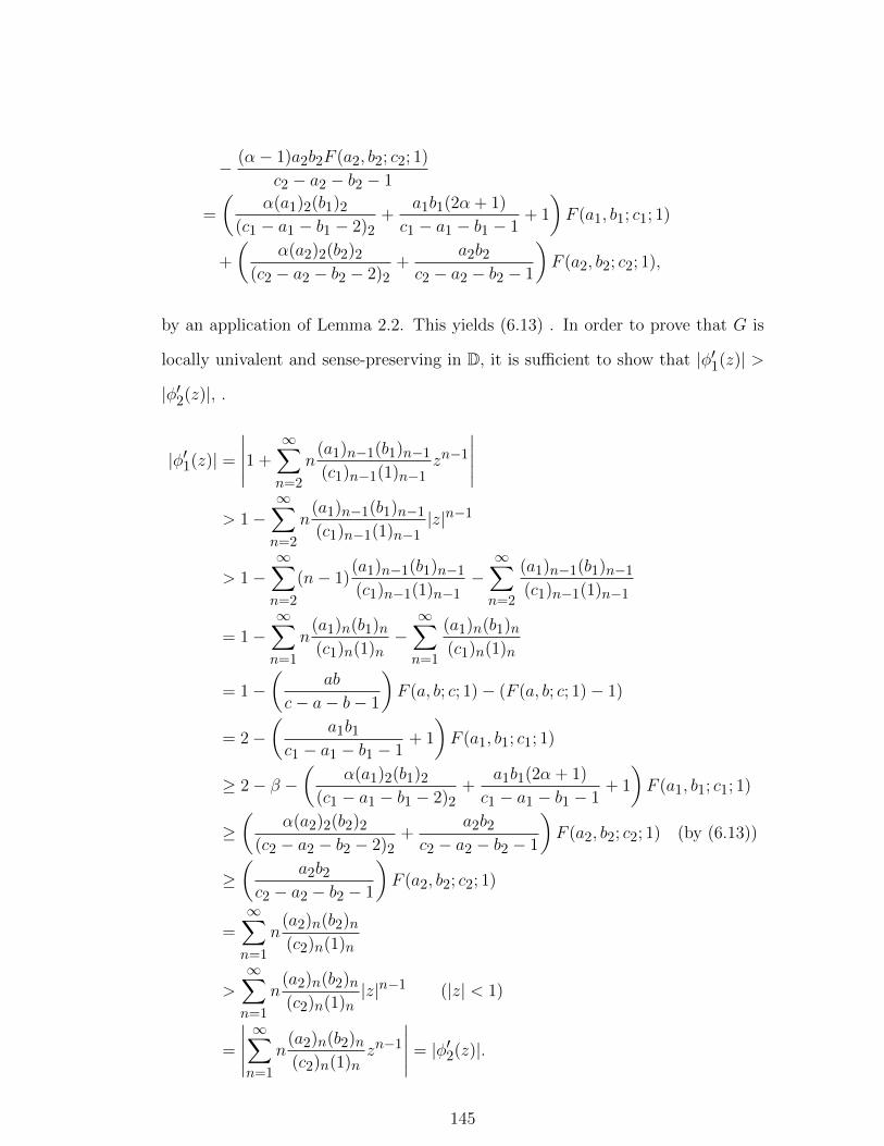
− (α− 1)a2b2F (a2, b2; c2; 1)
c2 − a2 − b2 − 1
=
(α(a1)2(b1)2
(c1 − a1 − b1 − 2)2+
a1b1(2α + 1)
c1 − a1 − b1 − 1+ 1
)F (a1, b1; c1; 1)
+
(α(a2)2(b2)2
(c2 − a2 − b2 − 2)2+
a2b2c2 − a2 − b2 − 1
)F (a2, b2; c2; 1),
by an application of Lemma 2.2. This yields (6.13) . In order to prove that G is
locally univalent and sense-preserving in D, it is sufficient to show that |φ′1(z)| >
|φ′2(z)|, .
|φ′1(z)| =
∣∣∣∣∣1 +∞∑n=2
n(a1)n−1(b1)n−1
(c1)n−1(1)n−1zn−1
∣∣∣∣∣> 1−
∞∑n=2
n(a1)n−1(b1)n−1
(c1)n−1(1)n−1|z|n−1
> 1−∞∑n=2
(n− 1)(a1)n−1(b1)n−1
(c1)n−1(1)n−1−∞∑n=2
(a1)n−1(b1)n−1
(c1)n−1(1)n−1
= 1−∞∑n=1
n(a1)n(b1)n(c1)n(1)n
−∞∑n=1
(a1)n(b1)n(c1)n(1)n
= 1−(
ab
c− a− b− 1
)F (a, b; c; 1)− (F (a, b; c; 1)− 1)
= 2−(
a1b1c1 − a1 − b1 − 1
+ 1
)F (a1, b1; c1; 1)
≥ 2− β −(
α(a1)2(b1)2
(c1 − a1 − b1 − 2)2+
a1b1(2α + 1)
c1 − a1 − b1 − 1+ 1
)F (a1, b1; c1; 1)
≥(
α(a2)2(b2)2
(c2 − a2 − b2 − 2)2+
a2b2c2 − a2 − b2 − 1
)F (a2, b2; c2; 1) (by (6.13))
≥(
a2b2c2 − a2 − b2 − 1
)F (a2, b2; c2; 1)
=∞∑n=1
n(a2)n(b2)n(c2)n(1)n
>
∞∑n=1
n(a2)n(b2)n(c2)n(1)n
|z|n−1 (|z| < 1)
=
∣∣∣∣∣∞∑n=1
n(a2)n(b2)n(c2)n(1)n
zn−1
∣∣∣∣∣ = |φ′2(z)|.
145
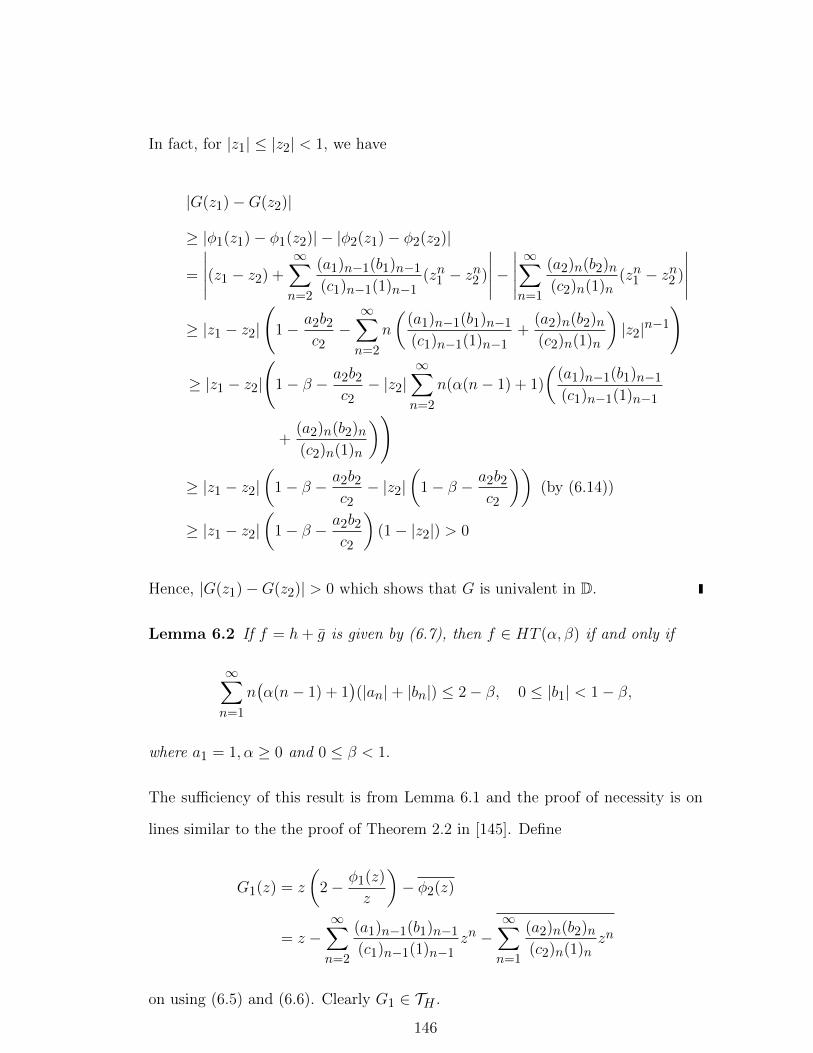
In fact, for |z1| ≤ |z2| < 1, we have
|G(z1)−G(z2)|
≥ |φ1(z1)− φ1(z2)| − |φ2(z1)− φ2(z2)|
=
∣∣∣∣∣(z1 − z2) +∞∑n=2
(a1)n−1(b1)n−1
(c1)n−1(1)n−1(zn1 − z
n2 )
∣∣∣∣∣−∣∣∣∣∣∞∑n=1
(a2)n(b2)n(c2)n(1)n
(zn1 − zn2 )
∣∣∣∣∣≥ |z1 − z2|
(1− a2b2
c2−∞∑n=2
n
((a1)n−1(b1)n−1
(c1)n−1(1)n−1+
(a2)n(b2)n(c2)n(1)n
)|z2|n−1
)
≥ |z1 − z2|
(1− β − a2b2
c2− |z2|
∞∑n=2
n(α(n− 1) + 1)
((a1)n−1(b1)n−1
(c1)n−1(1)n−1
+(a2)n(b2)n(c2)n(1)n
))
≥ |z1 − z2|(
1− β − a2b2c2− |z2|
(1− β − a2b2
c2
))(by (6.14))
≥ |z1 − z2|(
1− β − a2b2c2
)(1− |z2|) > 0
Hence, |G(z1)−G(z2)| > 0 which shows that G is univalent in D.
Lemma 6.2 If f = h+ g is given by (6.7), then f ∈ HT (α, β) if and only if
∞∑n=1
n(α(n− 1) + 1
)(|an|+ |bn|) ≤ 2− β, 0 ≤ |b1| < 1− β,
where a1 = 1, α ≥ 0 and 0 ≤ β < 1.
The sufficiency of this result is from Lemma 6.1 and the proof of necessity is on
lines similar to the the proof of Theorem 2.2 in [145]. Define
G1(z) = z
(2− φ1(z)
z
)− φ2(z)
= z −∞∑n=2
(a1)n−1(b1)n−1
(c1)n−1(1)n−1zn −
∞∑n=1
(a2)n(b2)n(c2)n(1)n
zn
on using (6.5) and (6.6). Clearly G1 ∈ TH .
146

Theorem 6.2 Let α ≥ 0, 0 ≤ β < 1, aj , bj > 0, cj > aj + bj + 2, for j = 1, 2 and
a2b2 < c2. G1 is in HT (α, β) if and only if (6.13) holds.
Proof. In view of Theorem 6.1, sufficiency of (6.13) is clear. We only need to show
the necessity of (6.13). If G1 ∈ HT (α, β), then G1 satisfies (6.14) by Lemma 6.2
and hence (6.13) holds.
Theorem 6.3 Let 0 ≤ β < 1, aj , bj > 0, cj > aj + bj + 1, for j = 1, 2 and
a2b2 < c2. A necessary and sufficient condition such that f ∗(φ1 +φ2) ∈ HT (α, β)
for f ∈ HT (α, β) is that
F (a1, b1; c1 : 1) + F (a2, b2; c2 : 1) ≤ 3 (6.15)
where φ1, φ2 are as defined, respectively, by (6.5) and (6.6).
Proof. Let f = h+ g ∈ HT (α, β), where h and g are given by (6.7). Then
(f ∗ (φ1 + φ2)
)(z) = h(z) ∗ φ1(z) + g(z) ∗ φ2(z)
= z −∞∑n=2
(a1)n−1(b1)n−1
(c1)n−1(1)n−1anz
n −∞∑n=1
(a2)n(b2)n(c2)n(1)n
bnzn.
In view of Lemma (6.2), we need to prove that (f ∗ (φ1 + φ2)) ∈ HT (α, β) if and
only if
∞∑n=1
n(α(n− 1) + 1)
((a1)n−1(b1)n−1
(c1)n−1(1)n−1an +
(a2)n(b2)n(c2)n(1)n
bn
)≤ 2− β. (6.16)
As an application of Lemma (6.2), we have
∞∑n=1
n(α(n− 1) + 1
)(an + bn) ≤ 2− β
or∞∑n=2
n(α(n− 1) + 1
)an +
∞∑n=1
n(α(n− 1) + 1
)bn ≤ 1− β
147

which implies
n(α(n− 1) + 1
)an ≤ 1− β and n
(α(n− 1) + 1
)bn ≤ 1− β.
Hence,
an ≤1− β
n(α(n− 1) + 1
) , n = 2, 3, · · · , and bn ≤1− β
n(α(n− 1) + 1
) , n = 1, 2, · · · .
(6.17)
Rewriting (6.16) we get
∞∑n=1
n(α(n− 1) + 1)
((a1)n−1(b1)n−1
(c1)n−1(1)n−1an +
(a2)n(b2)n(c2)n(1)n
bn
)≤ 2− β
or∞∑n=2
n(α(n− 1) + 1
)(a1)n−1(b1)n−1
(c1)n−1(1)n−1an
+∞∑n=1
n(α(n− 1) + 1
)(a2)n(b2)n(c2)n(1)n
bn ≤ 1− β. (6.18)
By applying (6.17), the left hand side of (6.18) is bounded above by
∞∑n=2
(1− β)(a1)n−1(b1)n−1
(c1)n−1(1)n−1+∞∑n=1
(1− β)(a2)n(b2)n(c2)n(1)n
= (1− β)
( ∞∑n=1
(a1)n(b1)n(c1)n(1)n
+∞∑n=1
(a2)n(b2)n(c2)n(1)n
)
= (1− β)(F (a1, b1; c1 : 1) + F (a2, b2; c2 : 1)− 2
).
The last expression is bounded above by (1 − β) if and only if (6.15) is satisfied.
This proves (6.16) and the results follows.
148

6.3 Integral Operators
Theorem 6.4 If aj , bj > 0 and cj > aj + bj + 1 for j = 1, 2, then a sufficient
condition for a function
G2(z) =
∫ z
0F (a1, b1; c1; t)dt+
∫ z
0
(F (a2, b2; c2; t)− 1
)dt
to be in HP (α, β) is that
(α(a1b1)
c1 − a1 − b1 − 1+ 1
)F (a1, b1; c1; 1)
+
(α(a2b2)
c2 − a2 − b2 − 1+ 1
)F (a2, b2; c2; 1) ≤ 3− β
where α ≥ 0 and 0 ≤ β < 1.
Proof. In view of Lemma 6.1, the function
G2(z) = z +∞∑n=2
(a1)n−1(b1)n−1
(c1)n−1(1)nzn +
∞∑n=2
(a2)n−1(b2)n−1
(c2)n−1(1)nzn
is in HP (α, β) if
∞∑n=2
n(α(n− 1) + 1)
((a1)n−1(b1)n−1
(c1)n−1(1)n+
(a2)n−1(b2)n−1
(c2)n−1(1)n
)≤ 1− β. (6.19)
By a computation we can write the left hand side of (6.19) as
∞∑n=1
(αn+ 1)
((a1)n(b1)n(c1)n(1)n
+(a2)n(b2)n(c2)n(1)n
)
= α
∞∑n=1
n(a1)n(b1)n(c1)n(1)n
+ α
∞∑n=1
n(a2)n(b2)n(c2)n(1)n
+∞∑n=1
(a1)n(b1)n(c1)n(1)n
+∞∑n=1
(a2)n(b2)n(c2)n(1)n
=αa1b1
c1 − a1 − b1 − 1F (a1, b1; c1; 1) +
αa2b2c2 − a2 − b2 − 1
F (a2, b2; c2; 1)
+ (F (a1, b1; c1; 1)− 1) + (F (a2, b2; c2; 1)− 1)
149
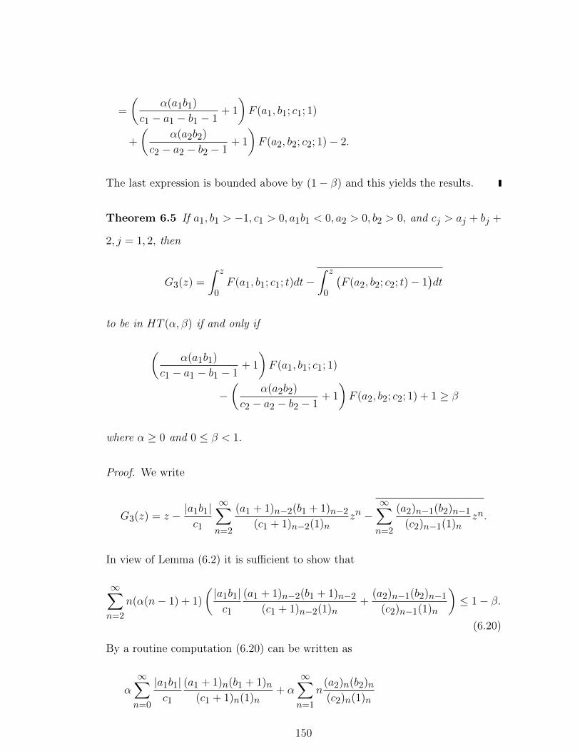
=
(α(a1b1)
c1 − a1 − b1 − 1+ 1
)F (a1, b1; c1; 1)
+
(α(a2b2)
c2 − a2 − b2 − 1+ 1
)F (a2, b2; c2; 1)− 2.
The last expression is bounded above by (1− β) and this yields the results.
Theorem 6.5 If a1, b1 > −1, c1 > 0, a1b1 < 0, a2 > 0, b2 > 0, and cj > aj + bj +
2, j = 1, 2, then
G3(z) =
∫ z
0F (a1, b1; c1; t)dt−
∫ z
0
(F (a2, b2; c2; t)− 1
)dt
to be in HT (α, β) if and only if
(α(a1b1)
c1 − a1 − b1 − 1+ 1
)F (a1, b1; c1; 1)
−(
α(a2b2)
c2 − a2 − b2 − 1+ 1
)F (a2, b2; c2; 1) + 1 ≥ β
where α ≥ 0 and 0 ≤ β < 1.
Proof. We write
G3(z) = z − |a1b1|c1
∞∑n=2
(a1 + 1)n−2(b1 + 1)n−2
(c1 + 1)n−2(1)nzn −
∞∑n=2
(a2)n−1(b2)n−1
(c2)n−1(1)nzn.
In view of Lemma (6.2) it is sufficient to show that
∞∑n=2
n(α(n− 1) + 1)
(|a1b1|c1
(a1 + 1)n−2(b1 + 1)n−2
(c1 + 1)n−2(1)n+
(a2)n−1(b2)n−1
(c2)n−1(1)n
)≤ 1− β.
(6.20)
By a routine computation (6.20) can be written as
α
∞∑n=0
|a1b1|c1
(a1 + 1)n(b1 + 1)n(c1 + 1)n(1)n
+ α∞∑n=1
n(a2)n(b2)n(c2)n(1)n
150

+∞∑n=1
|a1b1|c1
(a1 + 1)n−1(b1 + 1)n−1
(c1 + 1)n−1(1)n+∞∑n=1
(a2)n(b2)n(c2)n(1)n
≤ (1− β)
which implies
α
∞∑n=0
(a1 + 1)n(b1 + 1)n(c1 + 1)n(1)n
+αc1|a1b1|
∞∑n=1
n(a2)n(b2)n(c2)n(1)n
+∞∑n=0
(a1 + 1)n(b1 + 1)n(c1 + 1)n(1)n+1
+c1|a1b1|
∞∑n=1
(a2)n(b2)n(c2)n(1)n
≤ c1(1− β)
|a1b1|.
But, this is equivalent to
αc1a1b1
∞∑n=1
n(a1)n(b1)n(c1)n(1)n
+αc1|a1b1|
∞∑n=1
n(a2)n(b2)n(c2)n(1)n
+c1a1b1
∞∑n=1
(a1)n(b1)n(c1)n(1)n
+c1|a1b1|
∞∑n=1
(a2)n(b2)n(c2)n(1)n
≤ c1(1− β)
|a1b1|.
which yields
(α(a1b1)
c1 − a1 − b1 − 1+ 1
)F (a1, b1; c1; 1)
−(
α(a2b2)
c2 − a2 − b2 − 1+ 1
)F (a2, b2; c2; 1) + 1 ≥ β.
This completes the proof.
6.4 Coefficient Conditions for Incomplete Beta Function
In particular, the results parallel to Theorems 6.1, 6.3 ,6.4 and 6.5 may also be
obtained for the incomplete beta function ϕ(a, c; z) as defined by (6.4). Let
φ1(z) = ϕ(a1, c1; z) = z +∞∑n=2
(a1)n−1
(c1)n−1zn,
151

φ2(z) =1
zϕ(a2, c2; z)− 1 =
∞∑n=1
(a2)n(c2)n
zn, |a2| < |c2|.
Making use of
F (a1, 1; c1; 1) =c1 − 1
c1 − a1 − 1and F (a2, 1; c2; 1)− 1 =
a2
c2 − a2 − 1
the following theorems are obtained.
Theorem 6.6 If aj > 0 and cj > aj + 3 for j = 1, 2, then a sufficient condition
for G = φ1 + φ2 to be harmonic univalent in D with φ1 + φ2 ∈ HP (α, β), is that
(2α(a1)2
(c1 − a1 − 3)2+
2αa1 + c1 − 2
c1 − a1 − 2
)c1 − 1
c1 − a1 − 1
+
(2α(a2)2
(c2 − a2 − 3)2+
a2
c2 − a2 − 2
)c2 − 1
c2 − a2 − 1≤ 2− β (6.21)
where α ≥ 0 and 0 ≤ β < 1.
Note that the condition (6.21) is necessary and sufficient for G = φ1 + φ2 to be in
HT (α, β).
Theorem 6.7 Let 0 ≤ β < 1, aj > 0, cj > aj + 2, for j = 1, 2 and a2 < c2.
A necessary and sufficient condition such that f ∗ (φ1 + φ2) ∈ HT (α, β) for f ∈
HT (α, β) is that
c1 − 1
c1 − a1 − 1+
c2 − 1
c2 − a2 − 1≤ 3− β.
Theorem 6.8 If aj > 0 and cj > aj + 2 for j = 1, 2, then sufficient condition for
∫ z
0ϕ(a1, c1; t)dt+
∫ z
0
(ϕ(a2, c2; t)− 1
)dt
is in HP (α, β) is
(αa1
c1 − a1 − 2+ 1
)c1 − 1
c1 − a1 − 1+
(αa2
c2 − a2 − 2+ 1
)c2 − 1
c2 − a2 − 1≤ 3− β
152
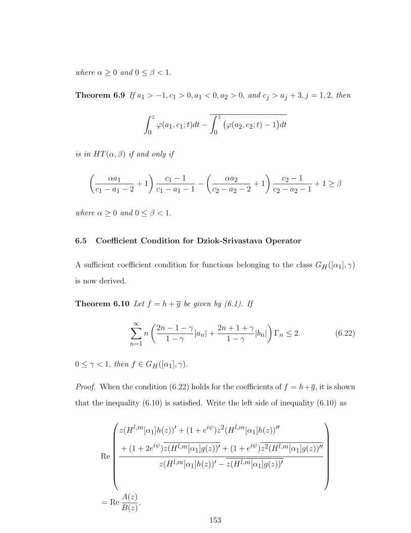
where α ≥ 0 and 0 ≤ β < 1.
Theorem 6.9 If a1 > −1, c1 > 0, a1 < 0, a2 > 0, and cj > aj + 3, j = 1, 2, then
∫ z
0ϕ(a1, c1; t)dt−
∫ z
0
(ϕ(a2, c2; t)− 1
)dt
is in HT (α, β) if and only if
(αa1
c1 − a1 − 2+ 1
)c1 − 1
c1 − a1 − 1−(
αa2
c2 − a2 − 2+ 1
)c2 − 1
c2 − a2 − 1+ 1 ≥ β
where α ≥ 0 and 0 ≤ β < 1.
6.5 Coefficient Condition for Dziok-Srivastava Operator
A sufficient coefficient condition for functions belonging to the class GH([α1], γ)
is now derived.
Theorem 6.10 Let f = h+ g be given by (6.1). If
∞∑n=1
n
(2n− 1− γ
1− γ|an|+
2n+ 1 + γ
1− γ|bn|)
Γn ≤ 2. (6.22)
0 ≤ γ < 1, then f ∈ GH([α1], γ).
Proof. When the condition (6.22) holds for the coefficients of f = h+g, it is shown
that the inequality (6.10) is satisfied. Write the left side of inequality (6.10) as
Re
z(H l,m[α1]h(z))′ + (1 + eiψ)z2(H l,m[α1]h(z))′′
+ (1 + 2eiψ)z(H l,m[α1]g(z))′ + (1 + eiψ)z2(H l,m[α1]g(z))′′
z(H l,m[α1]h(z))′ − z(H l,m[α1]g(z))′
= Re
A(z)
B(z),
153

where
A(z) = z(H l,m[α1]h(z))′ + (1 + eiψ)z2(H l,m[α1]h(z))′′
+ (1 + 2eiψ)z(H l,m[α1]g(z))′ + (1 + eiψ)z2(H l,m[α1]g(z))′′
and
B(z) = z(H l,m[α1]h(z))′ − z(H l,m[α1]g(z))′.
Since Re (w) ≥ γ if and only if |1 − γ + w| ≥ |1 + γ − w|, it is sufficient to show
that
|A(z) + (1− γ)B(z)| − |A(z)− (1 + γ)B(z)| ≥ 0. (6.23)
A computation shows that
A(z) + (1− γ)B(z)
= (2− γ)z(H l,m[α1]h(z))′ + (1 + eiψ)z2(H l,m[α1]h(z))′′
+ (2eiψ + γ)z(H l,m[α1]g(z))′ + (1 + eiψ)z2(H l,m[α1]g(z))′′
= (2− γ)z +∞∑n=2
((2− γ)n+ (1 + eiψ)(n2 − n)
)Γnanz
n
+∞∑n=1
((2eiψ + γ)n+ (1 + eiψ)n(n− 1)
)Γnbnz
n
and
A(z)− (1 + γ)B(z)
= −γz(H l,m[α1]h(z))′ + (1 + eiψ)z2(H l,m[α1]h(z))′′
+ (2 + 2eiψ + γ)z(H l,m[α1]g(z))′ + (1 + eiψ)z2(H l,m[α1]g(z))′′
= −γz +∞∑n=2
((n2 − n− γn) + eiψ(n2 − n)
)Γnanz
n
+∞∑n=1
((n2 + n+ γn) + eiψ(n2 + n)
)Γnbnz
n.
154

Hence,
|A(z) + (1− γ)B(z)| − |A(z)− (1 + γ)B(z)|
≥ |(2− γ)z| −
∣∣∣∣∣∞∑n=2
((2− γ)n+ (1 + eiψ)(n2 − n)
)Γnanz
n
∣∣∣∣∣−
∣∣∣∣∣∞∑n=1
((2eiψ + γ)n+ (1 + eiψ)n(n− 1)
)Γnbnz
n
∣∣∣∣∣−| − γz| −
∣∣∣∣∣∞∑n=2
((n2 − n− γn) + eiψ(n2 − n)
)Γnanz
n
∣∣∣∣∣−
∣∣∣∣∣∞∑n=1
((n2 + n+ γn) + eiψ(n2 + n)
)Γnbnz
n
∣∣∣∣∣≥ 2(1− γ)|z| −
∞∑n=2
2n(2n− 1− γ)Γn|an||z|n
−∞∑n=1
2n(2n+ 1 + γ)Γn|bn||z|n
≥ 2(1− γ)|z|
(1−
∞∑n=2
n2n− 1− γ
1− γΓn|an| −
∞∑n=1
n2n+ 1 + γ
1− γΓn|bn|
)
≥ 2(1− γ)|z|
(1 + |a1| −
∞∑n=1
n
(2n− 1− γ
1− γ|an|+
2n+ 1 + γ
1− γ|bn|)
Γn
)≥ 0
by the inequality
∞∑n=1
n
(2n− 1− γ
1− γ|an|+
2n+ 1 + γ
1− γ|bn|)
Γn ≤ 1 + |a1|. (6.24)
By the fact that 1 + |a1| ≤ 2, (6.24) yield (6.22) , which implies that f ∈
GH([α1], γ).
Now we obtain the necessary and sufficient condition for the function f = h+g
given by (6.7) to be in TH([α1], γ).
Theorem 6.11 Let f = h+g be given by (6.7). Then f ∈ TH([α1], γ) if and only
155

if∞∑n=1
n
(2n− 1− γ
1− γ|an|+
2n+ 1 + γ
1− γ|bn|)
Γn ≤ 2 (6.25)
where 0 ≤ γ < 1.
Proof. Since TH([α1], γ) ⊂ GH([α1, β1]), we only need to prove the necessary part
of the theorem. Assume that f ∈ TH([α1], γ), then by virtue of (6.10), we obtain
Re
(1− γ)z(H l,m[α1]h(z))′ + (1 + eiψ)z2(H l,m[α1]h(z))′′
+ (2eiψ + γ + 1)z(H l,m[α1]g(z))′ + (1 + eiψ)z2(H l,m[α1]g(z))′′
z(H l,m[α1]h(z))′ − z(H l,m[α1]g(z))′
≥ 0.
(6.26)
By taking the numerator of the left hand side of (6.26), a computation shows that
(1− γ)z
(1−
∞∑n=2
nΓn|an|zn−1
)+ (1 + eiψ)z2
(−∞∑n=2
n(n− 1)Γn|an|zn−2
)
+ (2eiψ + γ + 1)z
(−∞∑n=1
nΓn|bn|zn−1
)+ (1 + eiψ)z2
(−∞∑n=1
n(n− 1)Γn|bn|zn−2
)
= (1− γ)z −∞∑n=2
n((1− γ) + (1 + eiψ)(n− 1)
)Γn|an|zn
−∞∑n=1
n((2eiψ + γ + 1) + (1 + eiψ)(n− 1)
)Γn|bn|zn.
156

Therefore, by rewriting (6.26) it follows that
Re
(1− γ)−∞∑n=2
n(n(1 + eiψ)− eiψ − γ
)Γn|an|zn−1
−zz
∞∑n=1
n(n(1 + eiψ) + eiψ + γ
)Γn|bn|zn−1
1−∞∑n=2
nΓn|an|zn−1 +z
z
∞∑n=1
nΓn|bn|zn−1
≥ 0. (6.27)
This inequality (6.27) must hold for all values of z ∈ D and for real ψ, so that
on taking z = r < 1 and ψ = 0, (6.27) reduces to
(1− γ)−
( ∞∑n=2
n(2n− 1− γ)Γn|an|rn−1 +∞∑n=1
n(2n+ 1 + γ)Γn|bn|rn−1
)
1−∞∑n=2
Γn|an|rn−1 +∞∑n=1
Γn|bn|rn−1
≥ 0.
(6.28)
Letting r → 1− through real values, it follows that
(1− γ)−
( ∞∑n=2
n(2n− 1− γ)Γn|an|+∞∑n=1
n(2n+ 1 + γ)Γn|bn|
)
1−∞∑n=2
Γn|an|+∞∑n=1
Γn|bn|≥ 0
or
(1− γ)−
( ∞∑n=2
n(2n− 1− γ)Γn|an|+∞∑n=1
n(2n+ 1 + γ)Γn|bn|
)≥ 0. (6.29)
A computation shows that
(1− γ)−
( ∞∑n=2
n(2n− 1− γ)Γn|an|+∞∑n=1
n(2n+ 1 + γ)Γn|bn|
)
157

≥ (1− γ)
(1 + |a1| −
∞∑n=1
n
(2n− 1− γ
1− γ|an|+
2n+ 1 + γ
1− γ|bn|)
Γn
).
Hence, (6.29) is equivalent to
(1− γ)
(1 + |a1| −
∞∑n=1
n
(2n− 1− γ
1− γ|an|+
2n+ 1 + γ
1− γ|bn|)
Γn
)≥ 0 (6.30)
which holds true if
∞∑n=1
n
(2n− 1− γ
1− γ|an|+
2n+ 1 + γ
1− γ|bn|)
Γn ≤ 1 + |a1|. (6.31)
By the fact that 1 + |a1| ≤ 2, (6.31) yields (6.25). This completes the proof.
6.6 Extreme Points and Inclusion Results
We determine the extreme points of closed convex hulls of TH([α1], γ) denoted by
coTH([α1], γ).
Theorem 6.12 A function f(z) ∈ coTH([α1], γ) if and only if
f(z) =∞∑n=1
(Xnhn(z) + Yngn(z))
where
h1(z) = z, hn(z) = z − 1− γn(2n− 1− γ)Γn
zn; (n ≥ 2),
gn(z) = z − 1− γn(2n+ 1 + γ)Γn
zn; (n ≥ 2),
∞∑n=1
(Xn + Yn) = 1, Xn ≥ 0 and Yn ≥ 0.
In particular, the extreme points of TH([α1], γ) are hm and gm.
158

Proof. First, we note that for f as in theorem above, we may write
f(z) =∞∑n=1
(Xnhn(z) + Yngn(z))
= z
∞∑n=1
(Xn + Yn) + (h1(z)− z)X1 +∞∑n=2
(hn(z)− z)Xn
+∞∑n=1
(gn(z)− z)Yn
= z −∞∑n=2
1− γn(2n− 1− γ)Γn
Xnzn −
∞∑n=1
1− γn(2n+ 1 + γ)Γn
Ynzn
= z −∞∑n=2
Anzn −
∞∑n=1
Bnzn
where
An =1− γ
n(2n− 1− γ))ΓnXn and Bn =
1− γn(2n+ 1 + γ)Γn
Yn.
Therefore, in view of (6.25)
∞∑n=1
n
(2n− 1− γ
1− γAn +
2n+ 1 + γ
1− γBn
)Γn
= X1 +∞∑n=2
n(2n− 1− γ)Γn1− γ
(1− γ
n(2n− 1− γ))ΓnXn
)
+∞∑n=1
n(2n+ 1 + γ)Γn1− γ
(1− γ
n(2n+ 1 + γ)ΓnYn
)
= X1 +
(−X1 +
∞∑n=1
Xn
)+∞∑n=1
Yn
= 1 < 2
and hence f(z) ∈ coTH([α1], γ).
159

Conversely, suppose that f(z) ∈ coTH([α1], γ). Set
Xn =n(2n− 1− γ)Γn
1− γAn, (n ≥ 2), Yn =
n(2n+ 1 + γ)Γn1− γ
Bn, (n ≥ 1)
where∑∞n=1(Xn + Yn) = 1. Then
f(z) = z −∞∑n=2
Anzn −
∞∑n=1
Bnzn, An, Bn ≥ 0.
= z −∞∑n=2
1− γn(2n− 1− γ)Γn
Xnzn −
∞∑n=1
1− γn(2n+ 1 + γ)Γn
Ynzn
=∞∑n=1
(Xnhn(z) + Yngn(z))
as required.
Now we show that TH([α1], γ) is closed under convex combinations of its mem-
bers.
Theorem 6.13 The family TH([α1], γ) is closed under convex combinations.
Proof. For i = 1, 2, . . . , suppose that fi ∈ TH([α1], γ) where
fi(z) = z −∞∑n=2
|ai,n|zn −∞∑n=1
|bi,n|zn.
Then, by inequality (6.25)
∞∑n=1
n
(2n− 1− γ
1− γ|ai,n|+
2n+ 1 + γ
1− γ|bi,n|
)Γn ≤ 2 (6.32)
For∞∑i=1
ti = 1, 0 ≤ ti ≤ 1, the convex combination of fi may be written as
∞∑i=1
tifi(z) = z −∞∑n=2
( ∞∑i=1
ti|ai,n|
)zn −
∞∑n=1
( ∞∑i=1
ti|bi,n|
)zn.
160

Using the inequality (6.25), it follows that
∞∑n=1
n
(2n− 1− γ
1− γ
( ∞∑i=1
ti|ai,n|
)+
2n+ 1 + γ
1− γ
( ∞∑i=1
ti|bi,n|
))Γn
=∞∑i=1
ti
( ∞∑n=1
n
(2n− 1− γ
1− γ|ai,n|+
2n+ 1 + γ
1− γ|bi,n|
)Γn
)
≤ 2
and therefore∞∑i=1
tifi ∈ TH([α1], γ).
Theorem 6.14 For 0 ≤ δ ≤ γ < 1, let f(z) ∈ TH([α1], γ) and F (z) ∈ TH([α1], δ).
Then f(z) ∗ F (z) ∈ GH([α1], γ) ⊂ GH([α1], δ).
Proof. Let
f(z) = z −∞∑n=2
|an|zn −∞∑n=1
|bn|zn ∈ TH([α1], γ)
and
F (z) = z −∞∑n=2
|An|zn −∞∑n=1
|Bn|zn ∈ TH([α1], δ).
Then
f(z) ∗ F (z) = z +∞∑n=2
|an||An|zn +∞∑n=1
|bm||Bm|zn.
Note that |An| ≤ 1 and |Bn| ≤ 1 for n ≥ 2. Now we have
∞∑n=1
n
(2n− 1− δ
1− δ|an||An|+
2n+ 1 + δ
1− δ|bn||Bn|
)Γn
≤∞∑n=1
n
(2n− 1− δ
1− δ|an|+
2n+ 1 + δ
1− δ|bn|)
Γn
≤∞∑n=1
n
(2n− 1− γ
1− γ|an|+
2n+ 1 + γ
1− γ|bn|)
Γn
≤ 2
using Theorem 6.11 since f(z) ∈ TH([α1], γ) and 0 ≤ δ ≤ γ < 1. This proves that
161

f(z) ∗ F (z) ∈ GH([α1], γ) ⊂ GH([α1], δ).
Now, we examine a closure property of the class TH([α1], γ) under the gener-
alized Bernardi-Libera-Livingston integral operator F (z)
F (z) := (µ+ 1)
∫ 1
0tµ−1f(tz)dt (µ > −1)
which was defined earlier in Section 1.3.2, p. 22.
Theorem 6.15 Let f(z) ∈ TH([α1], γ). Then F (z) ∈ TH([α1], γ)
Proof. Let
f(z) = z −∞∑n=2
|an|zn −∞∑n=1
|bn|zn.
Then
F (z) = (µ+ 1)
∫ 1
0tµ−1
((tz)−
∞∑n=2
|an|(tz)n −∞∑n=1
|bn|(tz)n
)dt
= z −∞∑n=2
Anzn −
∞∑n=1
Bnzn
where
An =µ+ 1
µ+ n|an| and Bn =
µ+ 1
µ+ n|bn|.
Therefore, since f(z) ∈ TH([α1], γ),
∞∑n=1
n
(2n− 1− γ
1− γ
(µ+ 1
µ+ n|an|
)+
2n+ 1 + γ
1− γ
(µ+ 1
µ+ n|bn|))
Γn
≤∞∑n=1
n
(2n− 1− γ
1− γ|an|+
2n+ 1 + γ
1− γ|bn|)
Γn
≤ 2.
Therefore by Theorem 6.11, F (z) ∈ TH([α1], γ).
162

CONCLUSION
A modest attempt has been made in this thesis to introduce and study certain
classes of analytic and harmonic functions defined on the open unit disk D and
certain classes of meromorphic functions defined on the open punctured unit disk
D∗ using subordination, superordination and convolution.
• Closure properties under convolution of general classes of meromorphic mul-
tivalent functions with respect to n-ply symmetric, conjugate and symmetric
conjugate points are obtained.
• Differential subordination, differential superordination and sandwich-type
results are obtained for multivalent meromorphic functions associated with
the Dziok-Srivastava and Liu-Srivastava linear operator by investigating ap-
propriate classes of admissible functions.
• Sufficient conditions for Janowski starlikeness of analytic functions by mak-
ing use of the theory of differential subordination which are also applied to
Bernardi’s integral operator are obtained.
• New subclasses of harmonic functions defined through hypergeometric func-
tions are introduced and coefficient bounds, extreme points, inclusion results
and closure under an integral operator are discussed.
163

BIBLIOGRAPHY
[1] R. Aghalary, R. M. Ali, S. B. Joshi and V. Ravichandran,, Inequalities for
analytic functions defined by certain linear operators, Int. J. Math. Sci. 4
(2005), no. 2, 267–274.
[2] R. Aghalary and Gh. Azadi, The Dziok-Srivastava operator and k-uniformly
starlike functions, JIPAM. J. Inequal. Pure Appl. Math. 6 (2005), no. 2,
Article 52, 7 pp.
[3] R. Aghalary and J. M. Jahangiri, Inclusion relations for k-uniformly starlike
and related functions under certain integral operators, Bull. Korean Math.
Soc. 42 (2005), no. 3, 623–629.
[4] R. Aghalary, S. B. Joshi, R. N. Mohapatra and V. Ravichandran, Subordina-
tions for analytic functions defined by the Dziok-Srivastava linear operator,
Appl. Math. Comput. 187 (2007), no. 1, 13–19.
[5] O. P. Ahuja, Connections between various subclasses of planar harmonic
mappings involving hypergeometric functions, Appl. Math. Comput. 198
(2008), no. 1, 305–316.
[6] O. P. Ahuja, Planar harmonic convolution operators generated by hyper-
geometric functions, Integral Transforms Spec. Funct. 18 (2007), no. 3-4,
165–177.
[7] J. W. Alexander, Functions which map the interior of the unit circle upon
simple regions, Ann. of Math. (2) 17 (1915), no. 1, 12–22.
[8] R. M. Ali, N. E. Cho, V. Ravichandran and S. Sivaprasad Kumar, Differen-
tial subordination for functions associated with the lemniscate of Bernoulli,
Taiwanese J. Math. 16 (2012), no. 3, 1017–1026.
164

[9] R. M. Ali and V. Ravichandran, Differential subordination for meromorphic
functions defined by a linear operator, J. Anal. Appl. 2 (2004), no. 3, 149–
158.
[10] R. M. Ali, V. Ravichandran and N. Seenivasagan, Differential subordination
and superordination of analytic functions defined by the Dziok-Srivastava
linear operator, J. Franklin Inst. 347 (2010), no. 9, 1762–1781.
[11] R. M. Ali, V. Ravichandran and S. K. Lee, Subclasses of multivalent starlike
and convex functions, Bull. Belg. Math. Soc. Simon Stevin 16 (2009), no. 3,
385–394.
[12] R. M. Ali, V. Ravichandran and N. Seenivasagan, Differential subordination
and superordination of analytic functions defined by the multiplier transfor-
mation, Math. Inequal. Appl. 12 (2009), no. 1, 123–139.
[13] R. M. Ali, V. Ravichandran and N. Seenivasagan, Subordination and su-
perordination on Schwarzian derivatives, J. Inequal. Appl. 2008, Art. ID
712328, 18 pp.
[14] R. M. Ali, V. Ravichandran and N. Seenivasagan, On subordination and
superordination of the multiplier transformation for meromorphic functions,
Bull. Malays. Math. Sci. Soc. (2) 33 (2010), no. 2, 311–324.
[15] R. M. Ali, V. Ravichandran and N. Seenivasagan, Subordination and super-
ordination of the Liu-Srivastava linear operator on meromorphic functions,
Bull. Malays. Math. Sci. Soc. (2) 31 (2008), no. 2, 193–207.
[16] R. M. Ali, V. Ravichandran and N. Seenivasagan, Sufficient conditions for
Janowski starlikeness, Int. J. Math. Math. Sci. 2007, Art. ID 62925, 7 pp.
165

[17] R. M. Ali, V. Ravichandran and N. Seenivasagan, On Bernardi’s integral
operator and the Briot-Bouquet differential subordination, J. Math. Anal.
Appl. 324 (2006), no. 1, 663–668.
[18] R. M. Ali, A. O. Badghaish and V. Ravichandran, Multivalent functions
with respect to n-ply points and symmetric conjugate points, Comput. Math.
Appl. 60 (2010), no. 11, 2926–2935.
[19] R. M. Ali, M. Mahnaz, V. Ravichandran and K. G. Subramanian , Convolu-
tion properties of classes of analytic and meromorphic functions, J. Inequal.
Appl. 2010, Art. ID 385728, 14 pp.
[20] R. M. Ali and V. Singh, Convexity and starlikeness of functions defined by
a class of integral operators, Complex Variables Theory Appl. 26 (1995),
no. 4, 299–309.
[21] R. A. Al-Khal and H. A. Al-Kharsani, Harmonic hypergeometric functions,
Tamkang J. Math. 37 (2006), no. 3, 273–283.
[22] H. A. Al-Kharsani and R. A. Al-Khal, Univalent harmonic functions, JIPAM.
J. Inequal. Pure Appl. Math. 8 (2007), no. 2, Article 59, 8 pp.
[23] M. K. Aouf, H. M. Hossen and A. Y. Lashin, An application of certain
integral operators, J. Math. Anal. Appl. 248 (2000), no. 2, 475–481.
[24] M. K. Aouf, H. M. Hossen and A. Y. Lashin, An application of certain linear
operator, Bull. Korean Math. Soc. 37 (2000), no. 4, 765–770.
[25] M. K. Aouf and H. M. Hossen, New criteria for meromorphic p-valent starlike
functions, Tsukuba J. Math. 17 (1993), no. 2, 481–486.
[26] Y. Avcı and E. Z lotkiewicz, On harmonic univalent mappings, Ann. Univ.
Mariae Curie-Sk lodowska Sect. A 44 (1990), 1–7 (1991).
166
[27] S. D. Bernardi, Convex and starlike univalent functions, Trans. Amer. Math.
Soc. 135 (1969), 429–446.
[28] L. Bieberbach, Uber die Koeffizienten derjenigen Potenzreihen, welche eine
schlichte Abbildung des Einheitskreises vermitteln, Semesterberichte Preuss.
Akad. Wiss. 38 (1916), 940–955.
[29] D. A. Brannan and W. E. Kirwan, On some classes of bounded univalent
functions, J. London Math. Soc. (2) 1 (1969), 431–443.
[30] B. C. Carlson and D. B. Shaffer, Starlike and prestarlike hypergeometric
functions, SIAM J. Math. Anal. 15 (1984), no. 4, 737–745.
[31] R. Chand and P. Singh, On certain schlicht mappings, Indian J. Pure Appl.
Math. 10 (1979), no. 9, 1167–1174.
[32] J. Clunie and T. Sheil-Small, Harmonic univalent functions, Ann. Acad. Sci.
Fenn. Ser. A I Math. 9 (1984), 3–25.
[33] R. N. Das and P. Singh, On subclasses of schlicht mapping, Indian J. Pure
Appl. Math. 8 (1977), no. 8, 864–872.
[34] L. de Branges, A proof of the Bieberbach conjecture, Acta Math. 154 (1985),
no. 1-2, 137–152.
[35] P. L. Duren, Univalent functions, Grundlehren der Mathematischen Wis-
senschaften, 259, Springer, New York, 1983.
[36] P. Duren, Harmonic mappings in the plane, Cambridge Tracts in Mathemat-
ics, 156, Cambridge Univ. Press, Cambridge, 2004.
[37] J. Dziok and H. M. Srivastava, Classes of analytic functions associated with
the generalized hypergeometric function, Appl. Math. Comput. 103 (1999),
no. 1, 1–13.
167
[38] J. Dziok and H. M. Srivastava, Certain subclasses of analytic functions as-
sociated with the generalized hypergeometric function, Integral Transforms
Spec. Funct. 14 (2003), no. 1, 7–18.
[39] R. Md. El-Ashwah and D. K. Thomas, Some subclasses of close-to-convex
functions, J. Ramanujan Math. Soc. 2 (1987), no. 1, 85–100.
[40] B. A. Frasin and M. Darus, On certain analytic univalent functions, Int. J.
Math. Math. Sci. 25 (2001), no. 5, 305–310.
[41] P. R. Garabedian and M. A. Schiffer, A proof of the Bieberbach conjecture
for the fourth coefficient, J. Rational Mech. Anal. 4 (1955), 427–465.
[42] G. M. Goluzin, Geometric theory of functions of a complex variable, Trans-
lations of Mathematical Monographs, Vol. 26 Amer. Math. Soc., Providence,
RI, 1969.
[43] G. M. Goluzin, On distortion theorems in the theory of conformal mappings,
Mat. Sbornik N. S. 1(43) (1936), 127–135 (in Russian).
[44] A. W. Goodman, Univalent functions. Vol. I, Mariner, Tampa, FL, 1983.
[45] A. W. Goodman, On uniformly convex functions, Ann. Polon. Math. 56
(1991), no. 1, 87–92.
[46] A. W. Goodman, On uniformly starlike functions, J. Math. Anal. Appl. 155
(1991), no. 2, 364–370.
[47] I. Graham and G. Kohr, Geometric function theory in one and higher di-
mensions, Monographs and Textbooks in Pure and Applied Mathematics,
255, Dekker, New York, 2003.
[48] J. Hadamard, Theoreme sur les series entieres, Acta Math. 22 (1899), no. 1,
55–63.
168
[49] M. Haji Mohd, R. M. Ali, S. K. Lee and V. Ravichandran, Subclasses of
meromorphic functions associated with convolution, J. Inequal. Appl. 2009,
Art. ID 190291, 9 pp.
[50] W. K. Hayman, Multivalent functions, Cambridge Tracts in Mathematics
and Mathematical Physics, No. 48 Cambridge Univ. Press, Cambridge, 1958.
[51] Yu. E. Hohlov, Operators and operations in the class of univalent functions,
Izv. Vyss. Ucebn. Zaved. Mat. 10 (1978), 83–89.
[52] J. M. Jahangiri, Coefficient bounds and univalence criteria for harmonic
functions with negative coefficients, Ann. Univ. Mariae Curie-Sk lodowska
Sect. A 52 (1998), no. 2, 57–66.
[53] J. M. Jahangiri, Harmonic functions starlike in the unit disk, J. Math. Anal.
Appl. 235 (1999), no. 2, 470–477.
[54] J. M. Jahangiri, G. Murugusundaramoorthy and K. Vijaya, Starlikeness
of harmonic functions defined by Ruscheweyh derivatives, J. Indian Acad.
Math. 26 (2004), no. 1, 191–200.
[55] W. Janowski, Some extremal problems for certain families of analytic func-
tions. I, Ann. Polon. Math. 28 (1973), 297–326.
[56] S. B. Joshi and M. Darus, Unified treatment for harmonic univalent func-
tions, Tamsui Oxf. J. Math. Sci. 24 (2008), no. 3, 225–232.
[57] W. Kaplan, Close-to-convex schlicht functions, Michigan Math. J. 1 (1952),
169–185 (1953).
[58] Y. C. Kim and H. M. Srivastava, Inequalities involving certain families of
integral and convolution operators, Math. Inequal. Appl. 7 (2004), no. 2,
227–234.
169
[59] O. S. Kwon and N. E. Cho, Starlike and convex properties for hypergeometric
functions, Int. J. Math. Math. Sci. 2008, Art. ID 159029, 11 pp.
[60] H. Lewy, On the non-vanishing of the Jacobian in certain one-to-one map-
pings, Bull. Amer. Math. Soc. 42 (1936), no. 10, 689–692.
[61] J.-L. Li and S. Owa, Sufficient conditions for starlikeness, Indian J. Pure
Appl. Math. 33 (2002), no. 3, 313–318.
[62] R. J. Libera, Some classes of regular univalent functions, Proc. Amer. Math.
Soc. 16 (1965), 755–758.
[63] J. Liu and S. Owa, On certain meromorphic p-valent functions, Taiwanese
J. Math. 2 (1998), no. 1, 107–110.
[64] J.-L. Liu and H. M. Srivastava, Classes of meromorphically multivalent func-
tions associated with the generalized hypergeometric function, Math. Com-
put. Modelling 39 (2004), no. 1, 21–34.
[65] J.-L. Liu and H. M. Srivastava, Subclasses of meromorphically multivalent
functions associated with a certain linear operator, Math. Comput. Mod-
elling 39 (2004), no. 1, 35–44.
[66] A. E. Livingston, On the radius of univalence of certain analytic functions,
Proc. Amer. Math. Soc. 17 (1966), 352–357.
[67] K. Lowner, Untersuchungen uber schlichte konforme Abbildungen des Ein-
heitskreises. I, Math. Ann. 89 (1923), no. 1-2, 103–121.
[68] W. C. Ma and D. Minda, A unified treatment of some special classes of
univalent functions, in Proceedings of the Conference on Complex Analysis
(Tianjin, 1992), 157–169, Conf. Proc. Lecture Notes Anal., I Int. Press,
Cambridge, MA.
170
[69] E. P. Merkes and W. T. Scott, Starlike hypergeometric functions, Proc.
Amer. Math. Soc. 12 (1961), 885–888.
[70] W. C. Ma and D. Minda, Uniformly convex functions, Ann. Polon. Math.
57 (1992), no. 2, 165–175.
[71] S. S. Miller and P. T. Mocanu, Univalence of Gaussian and confluent hyper-
geometric functions, Proc. Amer. Math. Soc. 110 (1990), no. 2, 333–342.
[72] S. S. Miller and P. T. Mocanu, Differential subordinations, Monographs and
Textbooks in Pure and Applied Mathematics, 225, Dekker, New York, 2000.
[73] S. S. Miller and P. T. Mocanu, Subordinants of differential superordinations,
Complex Var. Theory Appl. 48 (2003), no. 10, 815–826.
[74] S. S. Miller, P. Mocanu and M. O. Reade, All α-convex functions are univa-
lent and starlike, Proc. Amer. Math. Soc. 37 (1973), 553–554.
[75] P. T. Mocanu, Une propriete de convexite generalisee dans la theorie de la
representation conforme, Mathematica (Cluj) 11 (34) (1969), 127–133.
[76] G. Murugusundaramoorthy, A class of Ruscheweyh-type harmonic univalent
functions with varying arguments, Southwest J. Pure Appl. Math. 2003,
no. 2, 90–95 (electronic).
[77] G. Murugusundaramoorthy and R. K. Raina, On a subclass of harmonic
functions associated with Wright’s generalized hypergeometric functions,
Hacet. J. Math. Stat. 38 (2009), no. 2, 129–136.
[78] Z. Nehari, Conformal mapping, McGraw-Hill, Inc., New York, Toronto, Lon-
don, 1952.
171

[79] R. Nevanlinna, Uber die konforme Abbildung Sterngebieten. Oeversikt av
Finska -Vetenskaps Societeten Forhandlingar 63(A), No. 6 (1921). FM 48-
403.
[80] I. R. Nezhmetdinov, A sharp lower bound in the distortion theorem for the
Sakaguchi class, J. Math. Anal. Appl. 242 (2000), no. 2, 129–134.
[81] K. Noshiro, On the theory of schlicht functions, J. Fac. Sci. Hokkaido Univ.
Jap(l), 2(1934-1935), 129-155.
[82] K. I. Noor and D. K. Thomas, Quasiconvex univalent functions, Internat. J.
Math. Math. Sci. 3 (1980), no. 2, 255–266.
[83] M. Nunokawa, M. Obradovic and S. Owa, One criterion for univalency, Proc.
Amer. Math. Soc. 106 (1989), no. 4, 1035–1037.
[84] M. Nunokawa, S. Owa, H. Saitoh, A. Ikeda and N. Koike,Some results for
strongly starlike functions, J. Math. Anal. Appl. 212 (1997), no. 1, 98–106.
[85] M. Nunokawa, S. Owa, H. Saitoh and N. Takahashi, On a strongly starlike-
ness criteria, Bull. Inst. Math. Acad. Sinica 31 (2003), no. 3, 195–199.
[86] M. Obradovic and S. Owa, On some criterions for starlikeness of order α,
Rend. Mat. Appl. (7) 8 (1988), no. 2, 283–289 (1989).
[87] M. Obradowic and N. Tuneski, On the starlike criteria defined by Silverman,
Zeszyty Nauk. Politech. Rzeszowskiej Mat. No. 24 (2000), 59–64 (2001).
[88] S. Owa, On the distortion theorems. I, Kyungpook Math. J. 18 (1978), no. 1,
53–59.
[89] S. Owa and H. M. Srivastava, Univalent and starlike generalized hypergeo-
metric functions, Canad. J. Math. 39 (1987), no. 5, 1057–1077.
172

[90] M. Ozawa, An elementary proof of the Bieberbach conjecture for the sixth
coefficient, Kodai Math. Sem. Rep. 21 (1969), 129–132.
[91] K. S. Padmanabhan, On sufficient conditions for starlikeness, Indian J. Pure
Appl. Math. 32 (2001), no. 4, 543–550.
[92] K. S. Padmanabhan and J. Thangamani, The effect of certain integral oper-
ators on some classes of starlike functions with respect to symmetric points,
Bull. Math. Soc. Sci. Math. R. S. Roumanie (N.S.) 26(74) (1982), no. 4,
355–360.
[93] H. S. Parihar, Inclusion relations for K-uniformly starlike functions and some
linear operator, Proyecciones 28 (2009), no. 2, 169–180.
[94] R. Parvatham, On Bernardi’s integral operators of certain classes of func-
tions, Kyungpook Math. J. 42 (2002), no. 2, 437–441.
[95] R. N. Pederson, A proof of the Bieberbach conjecture for the sixth coefficient,
Arch. Rational Mech. Anal. 31 (1968/1969), 331–351.
[96] R. Pederson and M. Schiffer, A proof of the Bieberbach conjecture for the
fifth coefficient, Arch. Rational Mech. Anal. 45 (1972), 161–193.
[97] C. Pommerenke, Univalent functions, Vandenhoeck & Ruprecht, Gottingen,
1975.
[98] S. Ponnusamy and F. Rønning, Starlikeness properties for convolutions in-
volving hypergeometric series, Ann. Univ. Mariae Curie-Sk lodowska Sect. A
52 (1998), no. 1, 141–155.
[99] S. Ponnusamy and F. Rønning, Geometric properties for convolutions of
hypergeometric functions and functions with the derivative in a halfplane,
Integral Transform. Spec. Funct. 8 (1999), no. 1-2, 121–138.
173
[100] S. Ponnusamy and S. Sabapathy, Geometric properties of generalized hyper-
geometric functions, Ramanujan J. 1 (1997), no. 2, 187–210.
[101] G. Polya and I. J. Schoenberg, Remarks on de la Vallee Poussin means and
convex conformal maps of the circle, Pacific J. Math. 8 (1958), 295–334.
[102] R. K. Raina and H. M. Srivastava, A new class of meromorphically multi-
valent functions with applications to generalized hypergeometric functions,
Math. Comput. Modelling 43 (2006), no. 3-4, 350–356.
[103] V. Ravichandran, Functions starlike with respect to n-ply symmetric, con-
jugate and symmetric conjugate points, J. Indian Acad. Math. 26 (2004),
no. 1, 35–45.
[104] V. Ravichandran and M. Darus, On a criteria for starlikeness, Int. Math. J.
4 (2003), no. 2, 119–125.
[105] V. Ravichandran, M. Darus and N. Seenivasagan, On a criteria for strong
starlikeness, Aust. J. Math. Anal. Appl. 2 (2005), no. 1, Art. 6, 12 pp.
[106] M. O. Reade, The coefficients of close-to-convex functions, Duke Math. J.
23 (1956), 459–462.
[107] M. I. S. Robertson, On the theory of univalent functions, Ann. of Math. (2)
37 (1936), no. 2, 374–408.
[108] F. Rønning, Integral representations of bounded starlike functions, Ann.
Polon. Math. 60 (1995), no. 3, 289–297.
[109] F. Rønning, On starlike functions associated with parabolic regions, Ann.
Univ. Mariae Curie-Sk lodowska Sect. A 45 (1991), 117–122 (1992).
[110] F. Rønning, Uniformly convex functions and a corresponding class of starlike
functions, Proc. Amer. Math. Soc. 118 (1993), no. 1, 189–196.
174

[111] M. Rosenblum and J. Rovnyak, Topics in Hardy classes and univalent func-
tions, Birkhauser Advanced Texts: Basler Lehrbucher. Birkhauser, Basel,
1994.
[112] T. Rosy et al., Goodman-type harmonic convex functions, J. Nat. Geom. 21
(2002), no. 1-2, 39–50.
[113] S. Ruscheweyh, Convolutions in geometric function theory, Seminaire de
Mathematiques Superieures, 83, Presses Univ. Montreal, Montreal, QC,
1982.
[114] S. Ruscheweyh, Linear operators between classes of prestarlike functions,
Comment. Math. Helv. 52 (1977), no. 4, 497–509.
[115] S. Ruscheweyh, New criteria for univalent functions, Proc. Amer. Math. Soc.
49 (1975), 109–115.
[116] St. Ruscheweyh and T. Sheil-Small, Hadamard products of Schlicht functions
and the Polya-Schoenberg conjecture, Comment. Math. Helv. 48 (1973),
119–135.
[117] St. Ruscheweyh and V. Singh, On the order of starlikeness of hypergeometric
functions, J. Math. Anal. Appl. 113 (1986), no. 1, 1–11.
[118] K. Sakaguchi, On a certain univalent mapping, J. Math. Soc. Japan 11
(1959), 72–75.
[119] T. N. Shanmugam, Convolution and differential subordination, Internat. J.
Math. Math. Sci. 12 (1989), no. 2, 333–340. MR0994916
[120] T. N. Shanmugam, C. Ramachandran and V. Ravichandran, Fekete-Szego
problem for subclasses of starlike functions with respect to symmetric points,
Bull. Korean Math. Soc. 43 (2006), no. 3, 589–598.
175

[121] T. Sheil-Small, Constants for planar harmonic mappings, J. London Math.
Soc. (2) 42 (1990), no. 2, 237–248.
[122] H. Silverman, Convex and starlike criteria, Int. J. Math. Math. Sci. 22
(1999), no. 1, 75–79.
[123] H. Silverman, Harmonic univalent functions with negative coefficients, J.
Math. Anal. Appl. 220 (1998), no. 1, 283–289.
[124] H. Silverman, Starlike and convexity properties for hypergeometric functions,
J. Math. Anal. Appl. 172 (1993), no. 2, 574–581.
[125] H. Silverman, Univalent functions with negative coefficients, Proc. Amer.
Math. Soc. 51 (1975), 109–116.
[126] S. Singh and S. Gupta, A differential subordination and starlikeness of ana-
lytic functions, Appl. Math. Lett. 19 (2006), no. 7, 618–627.
[127] S. Singh and S. Gupta, First order differential subordinations and starlike-
ness of analytic maps in the unit disc, Kyungpook Math. J. 45 (2005), no. 3,
395–404.
[128] S. Singh, S. Gupta and S. Singh, On certain results of differential subordi-
nation and superordination, Commun. Math. Anal. 6 (2009), no. 2, 21–32.
[129] H. M. Srivastava, Some families of fractional derivative and other linear
operators associated with analytic, univalent, and multivalent functions, in
Analysis and its applications (Chennai, 2000), 209–243, Allied Publ., New
Delhi.
[130] H. M. Srivastava and S. Owa, Some characterization and distortion the-
orems involving fractional calculus, generalized hypergeometric functions,
176

Hadamard products, linear operators, and certain subclasses of analytic func-
tions, Nagoya Math. J. 106 (1987), 1–28.
[131] H. M. Srivastava and J. Patel, Some subclasses of multivalent functions
involving a certain linear operator, J. Math. Anal. Appl. 310 (2005), no. 1,
209–228.
[132] H. M. Srivastava, D.-G. Yang and N.-E. Xu, Subordinations for multivalent
analytic functions associated with the Dziok-Srivastava operator, Integral
Transforms Spec. Funct. 20 (2009), no. 7-8, 581–606.
[133] B.A. Stephen, P. Nirmaladevi, T.V. Sudharsan and K.G. Subramanian, A
class of harmonic meromorphic functions with negative coefficients, Cham-
churi J. Math. 1 (2009), No. 1, 87–94.
[134] E. Study, Konforme Abbildung Einfachzusannmenhangender Bereiche. B. C
Teubner, Leipzig and Berlin, 1913. FM 44-755.
[135] S. Supramaniam et al., Convolution and differential subordination for multi-
valent functions, Bull. Malays. Math. Sci. Soc. (2) 32 (2009), no. 3, 351–360.
[136] A. Swaminathan, Hypergeometric functions in the parabolic domain, Tamsui
Oxf. J. Math. Sci. 20 (2004), no. 1, 1–16.
[137] A. Swaminathan, Certain sufficiency conditions on Gaussian hypergeometric
functions, JIPAM. J. Inequal. Pure Appl. Math. 5 (2004), no. 4, Article 83,
10 pp.
[138] J. Thangamani, On starlike functions with respect to symmetric points, In-
dian J. Pure Appl. Math. 11 (1980), no. 3, 392–405.
[139] N. Tuneski, On the quotient of the representations of convexity and starlike-
ness, Math. Nachr. 248/249 (2003), 200–203.
177

[140] Z.-G. Wang, A new subclass of quasi-convex functions with respect to k-
symmetric points, Lobachevskii J. Math. 19 (2005), 41–50 (electronic).
[141] Z.-G. Wang, Certain subclasses of close-to-convex and quasi-convex functions
with respect to K-symmetric points, Lobachevskii J. Math. 21 (2006), 73–83
(electronic).
[142] Z.-G. Wang, C.-Y. Gao and S.-M. Yuan, On certain subclasses of close-to-
convex and quasi-convex functions with respect to k-symmetric points, J.
Math. Anal. Appl. 322 (2006), no. 1, 97–106.
[143] Z.-G. Wang, Some subclasses of close-to-convex and quasi-convex functions,
Mat. Vesnik 59 (2007), no. 1-2, 65–73.
[144] S. E. Warschawski, On the higher derivatives at the boundary in conformal
mapping, Trans. Amer. Math. Soc. 38 (1935), no. 2, 310–340.
[145] S. Yalcin and M. Ozturk, A new subclass of complex harmonic functions,
Math. Inequal. Appl. 7 (2004), no. 1, 55–61.
[146] S.-M. Yuan, Z.-M. Liu and H. M. Srivastava, Some inclusion relationships
and integral-preserving properties of certain subclasses of meromorphic func-
tions associated with a family of integral operators, J. Math. Anal. Appl. 337
(2008), no. 1, 505–515.
178

PUBLICATIONS
1. R. Chandrashekar, G. Murugusundramoorthy, S. K. Lee and K. G. Subra-
manian, A Class of Complex-valued Harmonic Functions Defined by Dziok-
Srivastava Operator, Chamchuri Journal of Mathematics, 1 (2009), no. 2,
31–42.
2. R. Chandrashekar, S. K. Lee and K. G. Subramanian, Hypergeometric func-
tions and subclasses of harmonic mappings, Proceeding of the International
Conference on Mathematical Analysis 2010, Bangkok, 2010, pp. 95-103.
3. R. M. Ali, R. Chandrashekar, S. K. Lee, A. Swaminathan and V. Ravichan-
dran, Differential sandwich theorem for multivalent analytic functions asso-
ciated with the Dziok-Srivastava operator, Tamsui Oxf. J. Math. Sci. 27
(2011), no. 3, 327–350.
4. R. M. Ali, R. Chandrashekar, S. K. Lee, A. Swaminathan and V. Ravichan-
dran, Differential sandwich theorem for multivalent meromorphic functions
associated with the Liu-Srivastava operator, Kyungpook Math. J. 51 (2011),
no. 2, 217–232.
5. R. Chandrashekar, R. M. Ali, S. K. Lee and V. Ravichandran, Convolutions
of meromorphic multivalent functions with respect to n-ply points and sym-
metric conjugate points, Appl. Math. Comput. 218 (2011), no. 3, 723–728.
179