Subnational Trade Flows and State-Level Energy Intensity
34
Subnational Trade Flows and State-Level Energy Intensity Pandej Chintrakarn Southern Methodist University Daniel L. Millimet * Southern Methodist University Abstract In one strand of research, analysts examine trends in and the determinants of energy usage and intensity. In a second strand, researchers analyze the impact of trade flows on environmental outcomes. Recently, Cole (2006) bridges this gap, analyzing the impact of trade intensity on energy usage utilizing panel data at the country level. Here, we analyze the impact of subnational trade flows across U.S. states on state-level energy usage and intensity, controlling for the endogeneity of trade flows. Our findings indicate that an expansion of subnational trade at worst has no impact on state-level energy usage, and may actually re- duce energy usage (contrary to Cole’s country-level findings), although the impacts are not uniform across sectors. JEL: F18, Q4 Keywords: Bilateral Trade, Energy Intensity, Pollution Haven Hypothesis * Corresponding author: Daniel Millimet, Department of Economics, Box 0496, Southern Methodist University, Dallas, TX 75275-0496. Tel: (214) 768-3269. Fax: (214) 768-1821. E-mail: [email protected].
Transcript of Subnational Trade Flows and State-Level Energy Intensity
Subnational Trade Flows and State-Level Energy Intensity
Pandej Chintrakarn
Southern Methodist University
Daniel L. Millimet∗
Southern Methodist University
Abstract
In one strand of research, analysts examine trends in and the determinants of energy usage and intensity.In a second strand, researchers analyze the impact of trade flows on environmental outcomes. Recently,Cole (2006) bridges this gap, analyzing the impact of trade intensity on energy usage utilizing panel data atthe country level. Here, we analyze the impact of subnational trade flows across U.S. states on state-levelenergy usage and intensity, controlling for the endogeneity of trade flows. Our findings indicate that anexpansion of subnational trade at worst has no impact on state-level energy usage, and may actually re-duce energy usage (contrary to Cole’s country-level findings), although the impacts are not uniform acrosssectors.
JEL: F18, Q4Keywords: Bilateral Trade, Energy Intensity, Pollution Haven Hypothesis
∗Corresponding author: Daniel Millimet, Department of Economics, Box 0496, Southern Methodist University, Dallas, TX
75275-0496. Tel: (214) 768-3269. Fax: (214) 768-1821. E-mail: [email protected].
1 Introduction
Energy conservation is a continual topic of interest to policymakers, environmentalists, economists, and
others, in both the United States and abroad. It represents an issue that not only has ramifications on
the welfare of future generations, but also on the current generation. However, while anecdotal evidence
suggests that energy use responds to economic factors (e.g., the decline in energy intensity in the US
increased in magnitude after the oil shocks in the 1970s), relatively little is known about the determinants
of energy use. Nonetheless, the International Energy Agency forecasts that global energy use will increase
by 60% over current energy consumption (ICTSD [18]).
Within the US, only two studies (to our knowledge) analyze the spatial and temporal variation in
state-level energy intensity using regression techniques. Bernstein et al. [3] analyze panel data across US
states from 1977 to 1999, examining the role of Gross State Product (GSP), energy prices, and climate.
Metcalf [20] re-visits the issue, using panel data across US states from 1960 to 2001. The analyses point to
significant effects of prices and income on state-level energy intensity. Utilizing cross-country data, a few
recent studies have explored the role of trade openness and other economic factors on energy efficiency.
For instance, Fredriksson et al. [11] use panel data from 12 OECD countries to assess the role of political
corruption, lobbying, and industry size on energy intensity. Stern [25] explores the impact of NAFTA on
trends in energy intensity and per capita energy use in Canada, Mexico, and the US. Cole [6] uses panel
data across 32 countries to explore the role of trade on energy intensity and per capita energy use.
In this paper, we extend the line of inquiry begun in Bernstein et al. [3] and Metcalf [20], merging
the literature on interstate variation in energy intensity with the literature on trade and the environment
in general (e.g., Antweiler et al. [2]; Chintrakarn and Millimet [4]) and trade and energy intensity in
particular (as in Cole [6]). Specifically, we assess the impact of subnational ‘trade’ on state-level energy
intensity. There are several reasons why understanding the link between interstate trade and state-level
energy intensity is of relevance to policymakers and economists. First, as noted in Metcalf [20], variation
in the level of energy intensity across US states at a point in time is quite considerable, as is variation
across states in the change in energy intensity over time. Moreover, Metcalf [20] finds that most of the
variation is related to differences in energy efficiency, not differences in the sectoral composition of states.
The underlying causes of this variation in energy efficiency are at present a puzzle. Second, knowledge of
the determinants of energy use in the US will aid in forecasts of future energy demand. As is well known,
energy use – primarily fossil fuel consumption – contributes to air pollution, as well as global warming
through the emission of carbon. High energy consumption may also constitute a national security risk,
given the reliance of the US on foreign suppliers. In light of these and other externalities associated with
energy consumption, improved forecasts of future energy demand should prove valuable (see Metcalf [21]
1
for more discussion).
Third, policies aimed at energy conservation are most likely not cheap (see Metcalf [20] for greater
discussion). As such, identifying the determinants of energy use may illuminate more cost-effective energy
conservation strategies. For instance, in this analysis, we explore the role of interstate commerce on state-
level energy intensity. If expanded trade across states yields improvements (in a causal sense) in energy
intensity, then policies designed to facilitate interstate commerce would constitute one part of an overall
energy conservation strategy. Fourth, given the link between energy consumption and environmental
degradation, our analysis builds on previous work concerning the environmental impact of subnational
trade. In Chintrakarn and Millimet [4], the authors analyze the impact of interstate commerce on state-
level pollution of toxic releases, finding little evidence of harmful effects of trade on the environment on
average. Here, besides examining energy intensity instead of pollution levels, we extend the analysis in
Chintrakarn and Millimet [4] along three other dimensions. First, we now include a third wave of data on
interstate commerce (discussed below). Second, the (second-stage) empirical specification in the current
analysis differs from Chintrakarn and Millimet [4], and more in line with the theoretical literature (e.g.,
Antweiler et al. [2]) by accounting for the relative factor endowments of states (i.e., in theory, greater trade
intensity should increase (decrease) energy intensity in capital (labor) abundant states). Third, the first-
stage empirical specification of the gravity model for subnational trade – used to generate the instrument
for interstate trade – differs, following instead the method recently proposed in Santos Silva and Tenreyro
[24]. This method entails estimating the first-stage gravity model in levels (as opposed to logs). As noted
in Santos Silva and Tenreyro [24], estimating gravity models in logs may yield biased estimates of the
first-stage model, thereby invalidating the second-stage instrumental variable estimates.
The final motivation for the current analysis is that analyzing trade issues at the subnational level helps
inform the debate over the link between international trade and the environment. While some cross-country
evidence suggests that trade openness does not contribute to, and may actually mitigate, environmental
problems (e.g., Antweiler et al. [2]; Dean [9]; Harbaugh et al. [14]; Frankel and Rose [12]), issue remains
far from settled. Copeland and Taylor [8] (p. 7) state that “for the last ten years environmentalists
and the trade policy community have engaged in a heated debate over the environmental consequences of
liberalized trade.” Taylor [26] (p. 1) argues that this constitutes “one of the most important debates in
trade policy.” Moreover, the fact that Cole [6] finds a positive impact of trade intensity on per capita energy
consumption and energy intensity ceteris paribus indicates that the results from the trade and pollution
literature may not extend to the impact of trade on energy consumption. However, since Stern [25] fails to
find a detrimental impact of NAFTA on energy intensity, the link between international trade and energy
intensity is also unclear. Thus, the current analysis builds on a growing literature using subnational trade
data to assess open questions international trade arena since data obtained from a single country (i) ensures
2
consistent measurement of the variables of interest, and (ii) yields a more homogeneous sample, mitigating
concern over the omission of confounders (e.g., Wolf [28]; Hillberry and Hummels [17]; Combes et al. [7];
Millimet and Osang [22]; Knaap [19]).
To proceed, we follow Cole [6] and Antweiler et al. [2] and estimate several panel data specifications,
where state-level energy intensity depends on price, income, the capital-labor ratio, and trade intensity,
where the latter is allowed to be potentially endogenous. The findings are noteworthy. While consistent
with many previous works on the environmental effects of trade, our findings also confirm the role of
economic factors in explaining at least a portion of the cross-state variation in energy use in the US, as
discussed in Metcalf [20]. However, the results are in stark contrast with those in Cole [6], thus confirming
the importance of additional analysis. The remainder of the paper is organized as follows: Section 2
describes the empirical model and data. Section 3 presents empirical results. Section 4 concludes.
2 Methods & Data
2.1 Econometric Model
To assess the impact of subnational trade intensity on state-level energy intensity, we closely follow the
specification used in Cole [6], which is derived from the trade and environment framework developed in
Antweiler et al. [2]. Specifically, our estimating equation is
ln(Eit) = αt + α0 ln(Pit) + α1 ln(Yit) + α2 ln(Yit)2 + α3 ln(KLit) + α4 ln(KLit)2
+α5 ln(Yit) ln(KL) + α6 ln(Tit) + α7 ln(Tit) ln(RYit) + α8 ln(Tit) ln(RYit)2it
+α9 ln(Tit) ln(RKLit) + α10 ln(Tit) ln(RKLit)2 + εit (1)
where i indexes states, t indexes year, E is a measure of energy intensity, P is price, Y is one-period
lagged, three-year moving average of per capita Gross State Product (GSP), T is a measure of trade
intensity, RYit ≡ Yit/Y·t and RKLit ≡ KLit/KL·t, where the subscript “·t” indicates the average over all
i for year t, αt is a time-specific intercept, and ε is a mean zero error term.1 The error term is allowed
to be heteroskedastic in an arbitrary manner, and some specifications decompose the error term into a
state-specific fixed effect as well as a heteroskedastic idiosyncratic component.
Following Metcalf [20], we measure energy intensity as energy consumption per unit of economic activity
(discussed in more detail below). In addition to reporting the coefficient estimates, we also test the joint
significance of the five trade intensity variables, as well as report the elasticity of energy intensity with1Metcalf [20] allows for lagged energy prices to also impact current energy intensity. He tends to find sigificant effects of
current and one-period lagged prices. Given our sample size (discussed below), we include only current price in the analysis.
3
respect to Y , KL, and T (evaluated at the sample mean). These correspond to the technique, composition,
and trade elasticities, respectively. Standard errors for the elasticities are computed via the delta method.
As is well known, spatial and temporal variation in trade intensity is unlikely to be exogenous in general
(e.g., Copeland and Taylor [8], Frankel and Rose [12], Chintrakarn and Millimet [4]), and energy and other
environmental regulations and trade flows are likely to be jointly determined (Cole [6]; Ederington and
Minier [10]).2 To cope with the possible endogeneity of trade and per capita income, we instrument for
these variables in equation (1) using a General Methods of Moments (GMM) approach. The instruments
are equivalent to those utilized in Frankel and Rose [12], Chintrakarn and Millimet [4], and Cole [6].
Specifically, in the first-stage, we estimate a gravity model for bilateral shipments between pairs of states
and form the predicted level of shipments. Next, we aggregate the predicted values across bilateral trading
partners to obtain a prediction of total interstate shipments for a given state. In general, the gravity model
stipulates that trade is determined by the size (physical size as well as economic) of trading partners and
of distance between trading partners (physical distance as well as other determinants of ‘distance’ such
as a common border, landlocked status, common language, common currency, etc.). Here, we specify the
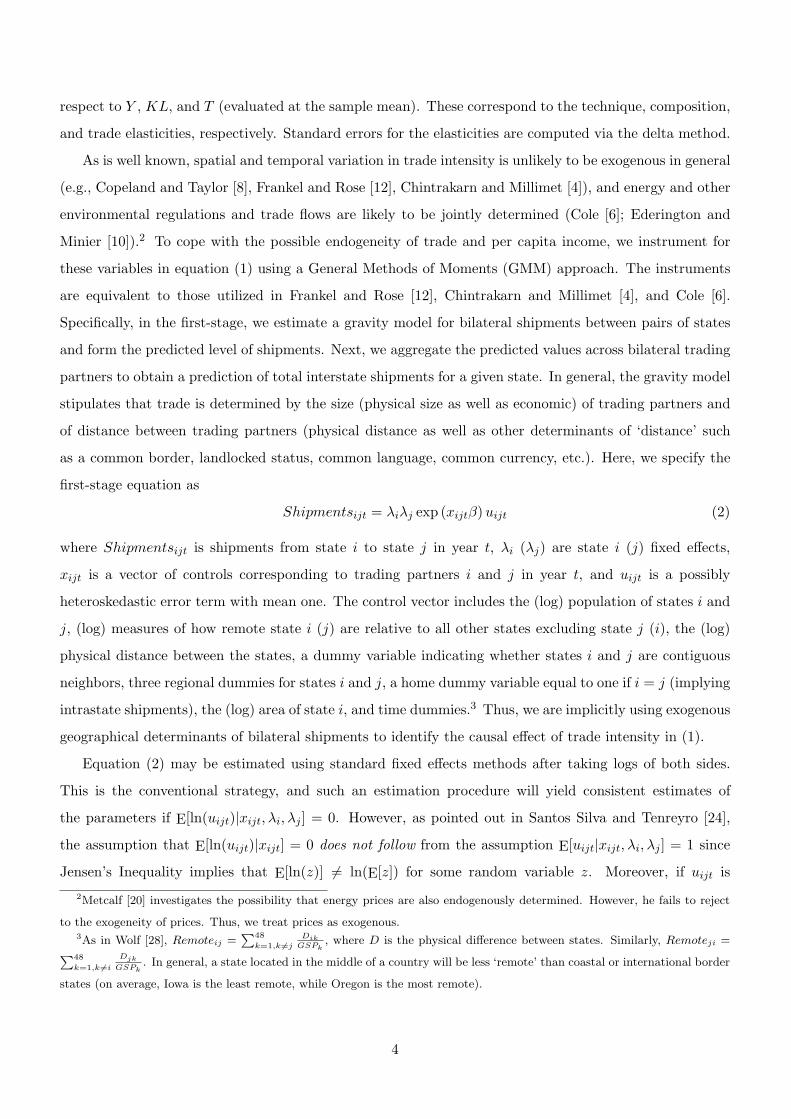
first-stage equation as
Shipmentsijt = λiλj exp (xijtβ)uijt (2)
where Shipmentsijt is shipments from state i to state j in year t, λi (λj) are state i (j) fixed effects,
xijt is a vector of controls corresponding to trading partners i and j in year t, and uijt is a possibly
heteroskedastic error term with mean one. The control vector includes the (log) population of states i and
j, (log) measures of how remote state i (j) are relative to all other states excluding state j (i), the (log)
physical distance between the states, a dummy variable indicating whether states i and j are contiguous
neighbors, three regional dummies for states i and j, a home dummy variable equal to one if i = j (implying
intrastate shipments), the (log) area of state i, and time dummies.3 Thus, we are implicitly using exogenous
geographical determinants of bilateral shipments to identify the causal effect of trade intensity in (1).
Equation (2) may be estimated using standard fixed effects methods after taking logs of both sides.
This is the conventional strategy, and such an estimation procedure will yield consistent estimates of
the parameters if E[ln(uijt)|xijt, λi, λj ] = 0. However, as pointed out in Santos Silva and Tenreyro [24],
the assumption that E[ln(uijt)|xijt] = 0 does not follow from the assumption E[uijt|xijt, λi, λj ] = 1 since
Jensen’s Inequality implies that E[ln(z)] 6= ln(E[z]) for some random variable z. Moreover, if uijt is
2Metcalf [20] investigates the possibility that energy prices are also endogenously determined. However, he fails to reject
to the exogeneity of prices. Thus, we treat prices as exogenous.3As in Wolf [28], Remoteij =
∑48
k=1,k 6=jDik
GSPk, where D is the physical difference between states. Similarly, Remoteji =
∑48
k=1,k 6=i
Djk
GSPk. In general, a state located in the middle of a country will be less ‘remote’ than coastal or international border
states (on average, Iowa is the least remote, while Oregon is the most remote).
4
heteroskedastic and its variance depends on xijt, then the expectation of ln(uijt) will in general also depend
on xijt, implying that fixed effects estimates based on the log-linear model will be biased. Instead, Santos
Silva and Tenreyro [24] proposes estimation in levels using a Poisson pseudo-maximum likelihood (PPML)
estimator. Henderson and Millimet [16] find that the estimation of (2) in levels using PPML outperforms
the log-linear model using US subnational trade data. Thus, we utilize the same estimator for the first-
stage.
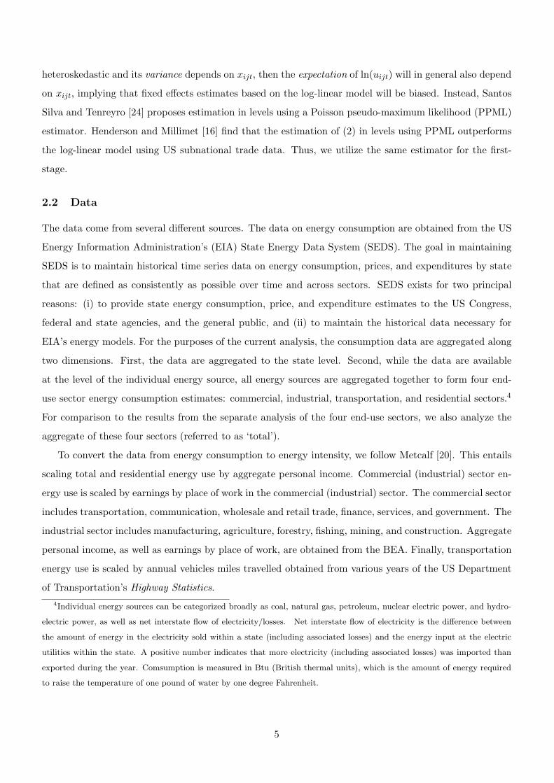
2.2 Data
The data come from several different sources. The data on energy consumption are obtained from the US
Energy Information Administration’s (EIA) State Energy Data System (SEDS). The goal in maintaining
SEDS is to maintain historical time series data on energy consumption, prices, and expenditures by state
that are defined as consistently as possible over time and across sectors. SEDS exists for two principal
reasons: (i) to provide state energy consumption, price, and expenditure estimates to the US Congress,
federal and state agencies, and the general public, and (ii) to maintain the historical data necessary for
EIA’s energy models. For the purposes of the current analysis, the consumption data are aggregated along
two dimensions. First, the data are aggregated to the state level. Second, while the data are available
at the level of the individual energy source, all energy sources are aggregated together to form four end-
use sector energy consumption estimates: commercial, industrial, transportation, and residential sectors.4
For comparison to the results from the separate analysis of the four end-use sectors, we also analyze the
aggregate of these four sectors (referred to as ‘total’).
To convert the data from energy consumption to energy intensity, we follow Metcalf [20]. This entails
scaling total and residential energy use by aggregate personal income. Commercial (industrial) sector en-
ergy use is scaled by earnings by place of work in the commercial (industrial) sector. The commercial sector
includes transportation, communication, wholesale and retail trade, finance, services, and government. The
industrial sector includes manufacturing, agriculture, forestry, fishing, mining, and construction. Aggregate
personal income, as well as earnings by place of work, are obtained from the BEA. Finally, transportation
energy use is scaled by annual vehicles miles travelled obtained from various years of the US Department
of Transportation’s Highway Statistics.4Individual energy sources can be categorized broadly as coal, natural gas, petroleum, nuclear electric power, and hydro-
electric power, as well as net interstate flow of electricity/losses. Net interstate flow of electricity is the difference between
the amount of energy in the electricity sold within a state (including associated losses) and the energy input at the electric
utilities within the state. A positive number indicates that more electricity (including associated losses) was imported than
exported during the year. Comsumption is measured in Btu (British thermal units), which is the amount of energy required
to raise the temperature of one pound of water by one degree Fahrenheit.
5
As noted in Metcalf [20], changes in energy intensity can arise for two reasons: changes in energy
efficiency and changes in economic activity. Changes in intensity due to energy efficiency refer to changes
in energy consumption per unit of economic activity within a particular sector. Changes in intensity due
to economic activity refer to changes in the allocation of economic activities across sectors. As a result,
analyzing the impact of trade on energy intensity by sector yields insight into trade effects on energy
efficiency, while analyzing the impact of trade on total energy intensity captures trade effects on efficiency
as well as economic activity.
The EIA also provides state-level energy price estimates. The estimates, expressed in nominal dollars
per million Btu, are consumption-weighted averages of the prices of the individual energy sources (see
footnote 4). The EIA calculation is performed by summing expenditures across the various energy sources
– coal (the sum of coking coal and steam coal), natural gas, petroleum (the sum of all petroleum products
used by the sector), wood, waste, alcohol fuels (in years when they are not included in motor gasoline),
and electricity – and dividing by total consumption.5
The inter- and intrastate shipments data are from the 1993, 1997 and 2002 Commodity Flow Survey
(CFS), collected by the Bureau of Transportation Statistics within the US Department of Transportation.
Chintrakarn and Millimet [4] utilize the 1993 and 1997 CFS data to explore the impact of subnational
trade on pollution; thus, we provide limited details and refer the reader to our previous work. The CFS
tracks all shipments across 25 two-digit and two three-digit SIC industries, measured in dollars and in tons.
Total shipments from one state to another (or within state) are reported. The CFS data have been used
frequently to assess the impact of borders on bilateral shipment patterns.6 With the CFS data in hand,
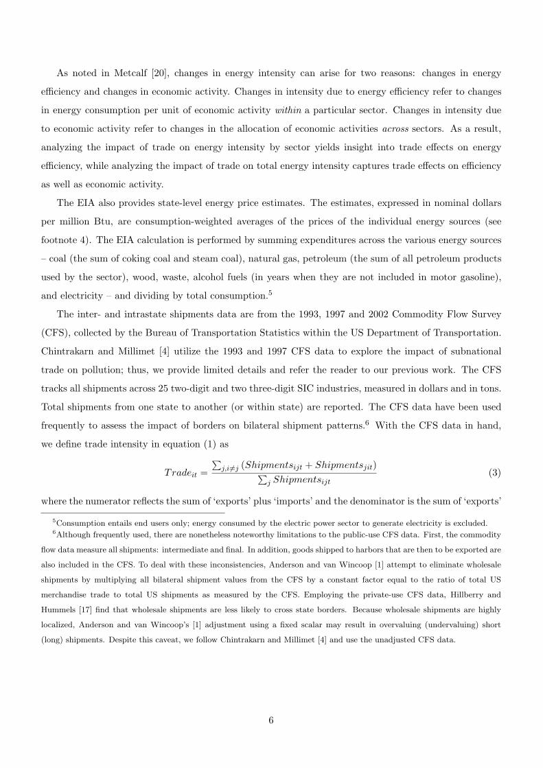
we define trade intensity in equation (1) as
Tradeit =∑
j,i6=j (Shipmentsijt + Shipmentsjit)∑j Shipmentsijt
(3)
where the numerator reflects the sum of ‘exports’ plus ‘imports’ and the denominator is the sum of ‘exports’
5Consumption entails end users only; energy consumed by the electric power sector to generate electricity is excluded.6Although frequently used, there are nonetheless noteworthy limitations to the public-use CFS data. First, the commodity
flow data measure all shipments: intermediate and final. In addition, goods shipped to harbors that are then to be exported are
also included in the CFS. To deal with these inconsistencies, Anderson and van Wincoop [1] attempt to eliminate wholesale
shipments by multiplying all bilateral shipment values from the CFS by a constant factor equal to the ratio of total US
merchandise trade to total US shipments as measured by the CFS. Employing the private-use CFS data, Hillberry and
Hummels [17] find that wholesale shipments are less likely to cross state borders. Because wholesale shipments are highly
localized, Anderson and van Wincoop’s [1] adjustment using a fixed scalar may result in overvaluing (undervaluing) short
(long) shipments. Despite this caveat, we follow Chintrakarn and Millimet [4] and use the unadjusted CFS data.
6
plus intrastate shipments.7,8
The final variable meriting serious discussion is the capital-labor ratio. Given the theoretical framework
in Antweiler et al. [2], measurement of the capital-labor ratio is crucial. However, the US Bureau of
Economic Analysis (BEA) only provides capital stock estimates for the US as a whole, not at the state-
level. To circumvent this shortcoming, we utilize two sources for state-level data on capital stocks. The
first source is Garofalo and Yamarik [13] (hereafter referred to as GY). GY construct US state-level capital
stocks from 1947 to 1996; a revised and extended series (through 2001) are available online.9 GY allocate
the national capital stock to the states using annual income shares. Specifically, for each of the nine one-
digit BEA industries, the authors allocate the national capital stock for that industry according to the
relative income generated within each state. Each state’s total capital stock estimate is given by the sum
of the industry estimates. Formally, the GY procedure is defined by the following equations:
kist =
(yist∑51
j=1 yjst
)kst (4)
kit =∑9
s=1kist (5)
where i indexes states, s indexes industry sectors, t indexes year, and k and y denote capital and income,
respectively, where kst is the national capital stock for industry s in year t.10
Concerned that this algorithm may not be yielding any new information, GY employ a regression
analysis of state income-to-capital ratios on the national income-to-capital ratio for the 1947-1996 period.
GY reject the null hypothesis that the coefficient on the national income-to-capial ratio equals one at the
p < 0.01 level. In addition, including state-level relative income shares for each industry in the regression
changes the coefficient on the national income-to-capital ratio very little, but the adjusted-R2 rises from
0.09 to 0.43. These results imply that more of the cross-state variation in the income-to-capital ratios is
attributable to variation in relative industry shares rather than the national income-to-capital ratio. More
importantly, the main findings in GY are consistent with long-held beliefs that constant returns to scale
is appropriate in a two factor model and the rate of convergence is approximately two percent per annum7Note, adjustment of a covariate by a constant factor, as in Anderson and van Wincoop [1], will affect the estimated
coefficient, but not inference regarding the statistical significance of the coefficient (i.e., the t-statistic does not change). Thus,
one should be cautious interpreting the magnitude of our results, but not the direction and statistical significance.8Due to data limitations and the specification of the gravity model in (2), we follow Combes et al. [7] and neglect shipments
between states and the rest of the world. We view this as a measurement error issue and since we utilize instrumental variable
techniques, this omission should not impact the results.
9See http://www.csulb.edu/˜syamarik/.10The nine industries with their BEA codes are farming (81); agricultural services, forestry, fishing, and other (100); mining
(200); construction (300); manufacturing (400); transportation (500); wholesale and retail trade (610); finance, insurance, and
real estate (700); and services (800). Data for y and kst are from the BEA.
7
among regions in the US. These results give us confidence that the GY state-level capital stock measure is
appropriate for our purposes. Finally, to construct the capital-labor ratio, state labor quantity is measured
by total full-time and part-time employment in each of the nine one-digit BEA industries. In our analysis,
we utilize GY’s capital-labor ratios from 1993, 1997, and 2001.11
The second source for data on state-level capital stocks is Cohen and Morrison [5] (hereafter referred to
as CM). To construct state-level private capital stocks for the period 1982-1996, CM apply the perpetual
inventory method to data on state-level new capital expenditures obtained from the US Census Bureau’s
Annual Survey of Manufactures (ASM), with the initial capital stock values (corresponding to the year
1982) taken from Morrison and Schwartz (1996). To form state-level capital-labor ratios, state labor
quantity is given by the number of full-time and part-time employees on the payrolls of these manufacturing
establishments (obtained from the ASM Geographic Area Statistics). In our analysis, we utilize CM’s
capital-labor ratios from 1993 and 1996.12 When comparing the two capital-labor ratio data series, the
CM method is more refined in the sense that the capital stocks are constructed using state-level data on
capital expenditures, instead of apportioning the national capital stock to the states. However, the GY
data enables us to utilize all three years of CFS data in the analysis, which is a significant benefit given
the sample size.
For the remaining variables, data on GSP come from the BEA, while state population is from the
Statistical Abstract of the United States (various editions). The measure of distance used in the first-stage
gravity model, equation (2), is borrowed from Wolf [28] and Millimet and Osang [22]. Summary statistics
are provided in Table 1.
3 Results
3.1 First-Stage Results
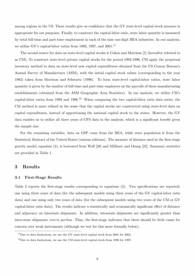
Table 2 reports the first-stage results corresponding to equations (2). Two specifications are reported;
one using three years of data (for the subsequent models using three years of the GY capital-labor ratio
data) and one using only two years of data (for the subsequent models using two years of the CM or GY
capital-labor ratio data). The results indicate a statistically and economically significant effect of distance
and adjacency on interstate shipments. In addition, intrastate shipments are significantly greater than
inter-state shipments ceteris paribus. Thus, the first-stage indicates that there should be little cause for
concern over weak instruments (although we test for this more formally below).
11Due to data limitations, we use the GY state-level capital stock from 2001 for 2002.
12Due to data limitations, we use the CM state-level capital stock from 1996 for 1997.
8

3.2 Second-Stage Results
3.2.1 Baseline Model
Estimates Results from our baseline model are presented in Tables 3 and 4, with Table 3 (4) displaying
the results obtained by estimating (1) via OLS (GMM). Each table presents the results using total energy
intensity, as well energy intensity for each of the four sectors. Moreover, for each measure of energy
intensity, Model I (II) uses the CM (GY) capital-labor ratio. Finally, in both tables, we utilize only two
periods of data – 1993 and 1997 – for comparability.
Turning to the OLS results for the total energy intensity (Table 3), three consistent findings emerge
regardless of which capital-labor ratio measure is used. First, consonant with Metcalf [20], the elasticity of
energy consumption is significantly, negatively related to price (Model I: α̂0 = −1.29, s.e. = 0.11; Model II:
α̂0 = −1.80, s.e. = 0.17). Second, consistent with Cole [6], we reject the null of no effect of trade intensity
(p = 0.00 in both models). Finally, consistent with Cole [6] and Antweiler et al. [2], we find a negative and
statistically significant technique elasticity (Model I: elasticity = -0.66, s.e. = 0.11; Model II: elasticity =
-0.82, s.e. = 0.23). Metcalf [20] also finds state-level energy intensity to be declining with income levels.
In terms of the remaining elasticities, we obtain positive and statistically significant composition and trade
elasticities using the CM capital-labor ratio; both are statistically insignificant at conventional levels using
the GY capital-labor ratio, although the trade elasticity is nearly identical to that obtained using the CM
measure. The positive elasticities obtained using the CM measure are consonant with the results in Cole
[6], however the magnitudes are much smaller. Thus, without accounting for the potential endogeneity of
subnational trade, we find a positive association on average between trade and energy intensity.
Examining the OLS results for the individual sectors yields several interesting findings. First, energy
intensity is negatively and significantly related to price in each sector and in each model, with energy
intensity in the industrial and transportation sectors being most price sensitive. Second, we reject the
null of no trade effects on energy intensity at the p < 0.10 level using both capital-labor ratios for the
industrial, commercial, and residential sectors. Third, the technique elasticity is negative in all eight
specifications, and statistically significant in six. Thus, within each sector, higher incomes are associated
with lower energy intensity. Fourth, the composition elasticity is positive and statistically significant in
six of the eight specifications as well. Finally, the trade elasticity is positive and relatively large for the
industrial sector using either capital-labor ratio, although it is statistically significant only when using the
CM measure (Model I: elasticity = 0.41, s.e. = 0.24; Model II: elasticity = 0.37, s.e. = 0.34). For the
remaining sectors, the trade elasticity is close to zero and statistically insignificant. Given the pattern of
results and the fact that industrial sector energy consumption comprises over one-third of total energy
consumption, it appears that most of the positive association between trade and total energy intensity is
9
due to a positive association between trade and energy inefficiency in the industrial sector, and not due to
correlation between trade intensity and the sectoral composition of economic activity.
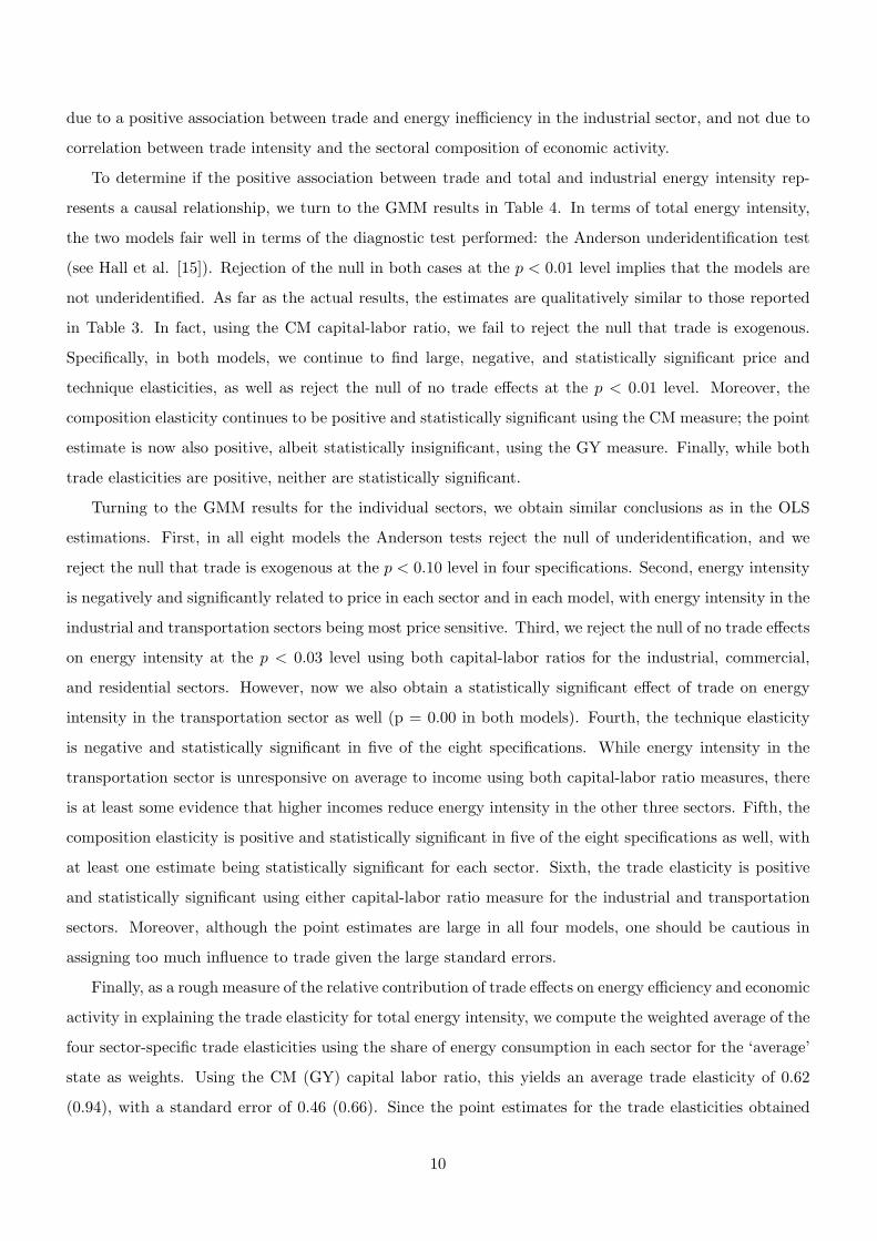
To determine if the positive association between trade and total and industrial energy intensity rep-
resents a causal relationship, we turn to the GMM results in Table 4. In terms of total energy intensity,
the two models fair well in terms of the diagnostic test performed: the Anderson underidentification test
(see Hall et al. [15]). Rejection of the null in both cases at the p < 0.01 level implies that the models are
not underidentified. As far as the actual results, the estimates are qualitatively similar to those reported
in Table 3. In fact, using the CM capital-labor ratio, we fail to reject the null that trade is exogenous.
Specifically, in both models, we continue to find large, negative, and statistically significant price and
technique elasticities, as well as reject the null of no trade effects at the p < 0.01 level. Moreover, the
composition elasticity continues to be positive and statistically significant using the CM measure; the point
estimate is now also positive, albeit statistically insignificant, using the GY measure. Finally, while both
trade elasticities are positive, neither are statistically significant.
Turning to the GMM results for the individual sectors, we obtain similar conclusions as in the OLS
estimations. First, in all eight models the Anderson tests reject the null of underidentification, and we
reject the null that trade is exogenous at the p < 0.10 level in four specifications. Second, energy intensity
is negatively and significantly related to price in each sector and in each model, with energy intensity in the
industrial and transportation sectors being most price sensitive. Third, we reject the null of no trade effects
on energy intensity at the p < 0.03 level using both capital-labor ratios for the industrial, commercial,
and residential sectors. However, now we also obtain a statistically significant effect of trade on energy
intensity in the transportation sector as well (p = 0.00 in both models). Fourth, the technique elasticity
is negative and statistically significant in five of the eight specifications. While energy intensity in the
transportation sector is unresponsive on average to income using both capital-labor ratio measures, there
is at least some evidence that higher incomes reduce energy intensity in the other three sectors. Fifth, the
composition elasticity is positive and statistically significant in five of the eight specifications as well, with
at least one estimate being statistically significant for each sector. Sixth, the trade elasticity is positive
and statistically significant using either capital-labor ratio measure for the industrial and transportation
sectors. Moreover, although the point estimates are large in all four models, one should be cautious in
assigning too much influence to trade given the large standard errors.
Finally, as a rough measure of the relative contribution of trade effects on energy efficiency and economic
activity in explaining the trade elasticity for total energy intensity, we compute the weighted average of the
four sector-specific trade elasticities using the share of energy consumption in each sector for the ‘average’
state as weights. Using the CM (GY) capital labor ratio, this yields an average trade elasticity of 0.62
(0.94), with a standard error of 0.46 (0.66). Since the point estimates for the trade elasticities obtained
10
using total energy intensity are much smaller (CM: elasticity = 0.24, s.e. = 0.22; GY: elasticity = 0.36,
s.e. = 0.41), this implies that greater trade intensity may shift state economic activity to sectors in which
energy intensity is not affected by trade (i.e., the commercial and residential sectors). However, given the
standard errors, we also cannot reject that there is no impact of trade on the composition of economic
activity. Nonetheless, we do conclude that trade raises energy intensity (i.e., decreases energy efficiency)
in the industrial and transportation sectors.
In the end, then, the baseline model treating trade as endogenous confirms the cross-country result in
Cole [6]; trade causes energy intensity to rise on average. However, the impact is not homogeneous across
sectors as the increase in intensity is concentrated in the industrial and transportation sectors. Moreover,
while some of our empirical results are sensitive to which measure of the state-level capital-labor ratio is
used, this conclusion is not. Finally, our analysis also confirms the results in Metcalf [20] that state-level
energy intensity is quite sensitive to price and income, with the effects of both being negative on average.
The positive effect of trade on energy intensity on average is surprising given the results in Chintrakarn
and Millimet [4], which find negative effects on average of state-level trade intensity on toxic releases in
general, and toxic releases to the air in particular. If this baseline result holds up to the robustness tests
discussed below, this implies that the beneficial effects of greater interstate trade on toxic releases is more
than sufficient to offset the higher level of energy intensity.
Heterogeneous Effects Prior to discussing the sensitivity tests, we delve a bit deeper into the results
from the baseline model. One of the primary insights of Antweiler et al. [2] is that trade liberalization has
differential effects on the environment depending on whether such liberalization leads to greater imports
or exports of pollution-intensive goods. While the empirical model allows for such heterogeneity – as the
impact of trade intensity is allowed to vary non-linearly with relative income and relative factor endowments
– the preceding results focus on the average impact of trade on energy intensity. To assess this heterogeneity,
rather than simply focusing on average effects, we use the results from Table 4 to calculate the trade
elasticity of energy intensity for each state-year observation. Table A1 in the Appendix reports the average
elasticity for each state and sector, along with its ranking, using both capital-labor ratio measures.
Examining the elasticities for total energy intensity using CM’s capital-labor ratio, we find only three
states with negative trade elasticities, and the majority of states are clustered around the elasticity com-
puted at the mean reported in Table 4 (elasticity = 0.24, s.e. = 0.22). Delaware has the largest elasticity,
with a point estimate of 0.72; Vermont, Wyoming, and Louisiana have the three negative elasticities (-0.06,
-0.39, and -0.60, respectively). Using GY’s capital-labor ratio yields much more heterogeneity across the
states. In particular, we find more instances of negative trade elasticities (14), and several instances of
extremely large positive elasticities (e.g., Wyoming, New York, and Connecticut each have an elasticity
11
above 1.50). Moreover, we note that while the results using the two capital-labor ratio measures are pre-
dominantly similar, there are a few large discrepancies. For example, Wyoming’s elasticity changes from
-0.39 (ranking = 47) to 2.86 (ranking = 1); Oklahoma’s elasticity changes from 0.32 (ranking = 9) to -0.29
(ranking = 48). However, because we do not report standard errors for these averages, one should view
these discrepancies with caution.
Turning to the industrial sector, we obtain results broadly consistent with the those obtained using total
energy intensity. However, the point estimates do exhibit substantially greater variation. As when using
total energy intensity, we obtain three negative trade elasticities using CM’s capital-labor ratio; only four
using GY’s measure. Across both measures, Mississippi’s elasticity is consistently very large (CM: elasticity
= 4.90, ranking = 1; GY: elasticity = 4.99, ranking = 2), whereas Louisiana’s is consistently low (CM:
elasticity = -1.74, ranking = 47; GY: elasticity = -0.30, ranking = 48). The results for the transportation
sector – the other sector with a statistically significant trade elasticity computed at the mean in Table
3 – are fairly similar to those for the industrial sector, although there are more instances of negative
elasticities. Specifically, using CM’s (GY’s) capital-labor ratio, we obtain 13 (five) states with negative
elasticities. However, using CM’s capital-labor ratio, the five states with the highest trade elasticities in
the industrial sector, continue to have the five largest elasticities in the transportation sector (Mississippi,
Montana, West Virginia, Arkansas, and Oklahoma).
For the commercial sector, the distribution of elasticities obtained using the CM measure is relatively
symmetric around the trade elasticity computed at the mean reported in Table 4 (elasticity = 0.48, s.e. =
0.32); there are eight states with negative elasticities, and eight states with elasticities above unity. The
distribution obtained using the GY measure is more skewed, with a long upper tail. While eight states have
negative elasticities as with the CM measure, four (ten) states have an elasticity above 1.90 (one). Finally,
for the residential sector, we find the greatest evidence of a beneficial effect of interstate trade on energy
intensity; we also find the most amount of consistency across the two capital-labor ratios. Using the CM
(GY) capital-labor ratio, only 17 (15) of 48 states have positive trade elasticities. In terms of particular
states, Montana, West Virginia, and Mississippi have the lowest point estimates across both capital-labor
ratio measures, with elasticities below -1.80; Connecticut is the only state with an elasticity greater than
unity according to both capital-labor ratio measures.
In sum, there is substantial variation in the point estimates of the state-specific trade elasticities, as well
as variation in the rankings of states across the different sectors. For instance, Mississippi consistently ranks
in the top ten states in terms of largest trade elasticity in the industrial, commercial, and transportation
sectors, but is among the bottom two states in the residential sector. Illinois, on the other hand, has
the eleventh highest trade elasticity overall using either capital-labor ratio (CM: elasticity = 0.30; GY:
elasticity = 0.51), but predominantly ranks in the bottom one-third of states in the industrial, commercial,
12
and transportation sectors, and in the top ten in the residential sector (CM: elasticity = 0.42; GY: elasticity
= 0.51). That said, the results indicate that the elasticities computed at the mean reported in Table 4 are
not driven by one or two states, but rather represent a good description of the general effects of trade on
energy intensity.
3.2.2 Sensitivity Analysis
As stated previously, the positive effect of trade on energy intensity on average found in the baseline model
is unexpected in light of the results obtained in Chintrakarn and Millimet [4]. To assess the robustness of
the baseline findings, we conduct a number of sensitivity analyses. We discuss each in turn.
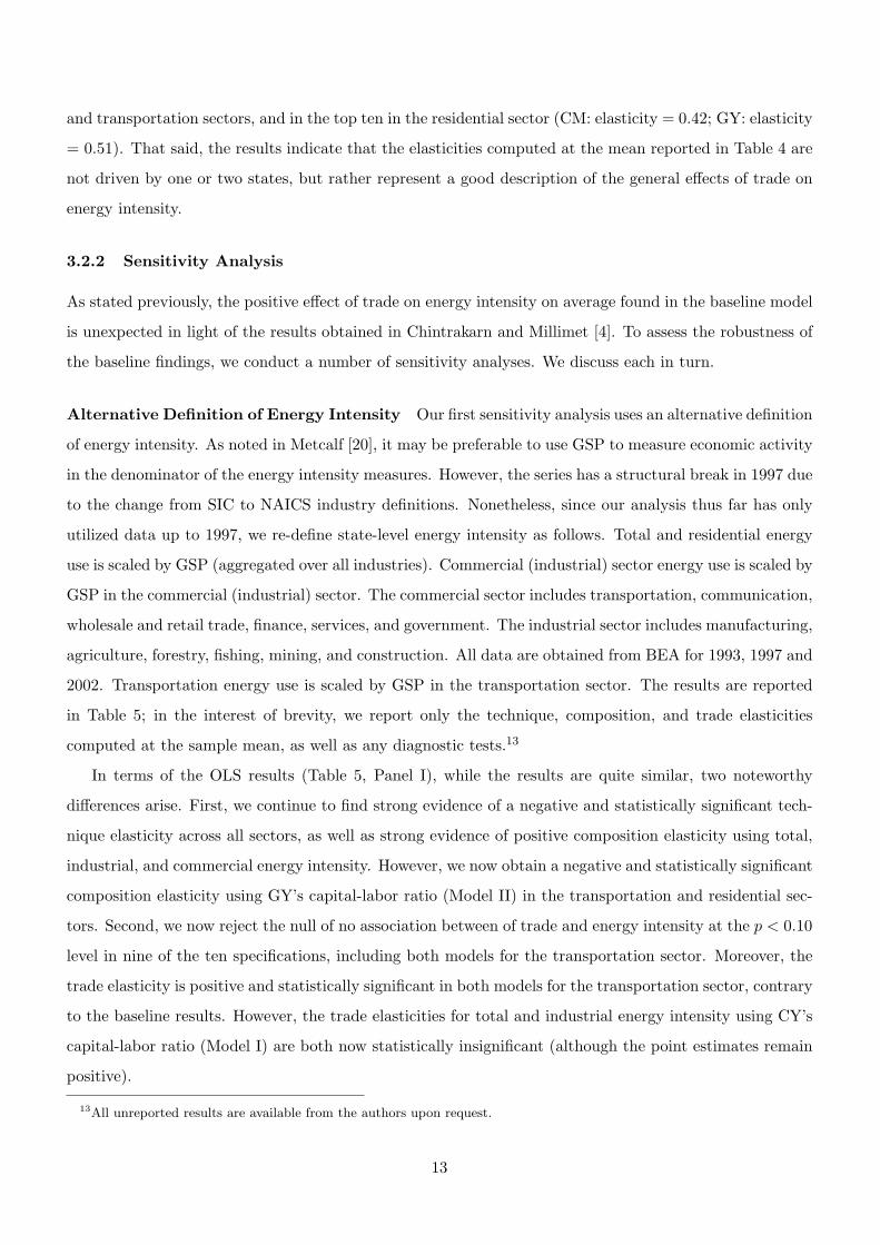
Alternative Definition of Energy Intensity Our first sensitivity analysis uses an alternative definition
of energy intensity. As noted in Metcalf [20], it may be preferable to use GSP to measure economic activity
in the denominator of the energy intensity measures. However, the series has a structural break in 1997 due
to the change from SIC to NAICS industry definitions. Nonetheless, since our analysis thus far has only
utilized data up to 1997, we re-define state-level energy intensity as follows. Total and residential energy
use is scaled by GSP (aggregated over all industries). Commercial (industrial) sector energy use is scaled by
GSP in the commercial (industrial) sector. The commercial sector includes transportation, communication,
wholesale and retail trade, finance, services, and government. The industrial sector includes manufacturing,
agriculture, forestry, fishing, mining, and construction. All data are obtained from BEA for 1993, 1997 and
2002. Transportation energy use is scaled by GSP in the transportation sector. The results are reported
in Table 5; in the interest of brevity, we report only the technique, composition, and trade elasticities
computed at the sample mean, as well as any diagnostic tests.13
In terms of the OLS results (Table 5, Panel I), while the results are quite similar, two noteworthy
differences arise. First, we continue to find strong evidence of a negative and statistically significant tech-
nique elasticity across all sectors, as well as strong evidence of positive composition elasticity using total,
industrial, and commercial energy intensity. However, we now obtain a negative and statistically significant
composition elasticity using GY’s capital-labor ratio (Model II) in the transportation and residential sec-
tors. Second, we now reject the null of no association between of trade and energy intensity at the p < 0.10
level in nine of the ten specifications, including both models for the transportation sector. Moreover, the
trade elasticity is positive and statistically significant in both models for the transportation sector, contrary
to the baseline results. However, the trade elasticities for total and industrial energy intensity using CY’s
capital-labor ratio (Model I) are both now statistically insignificant (although the point estimates remain
positive).
13All unreported results are available from the authors upon request.
13
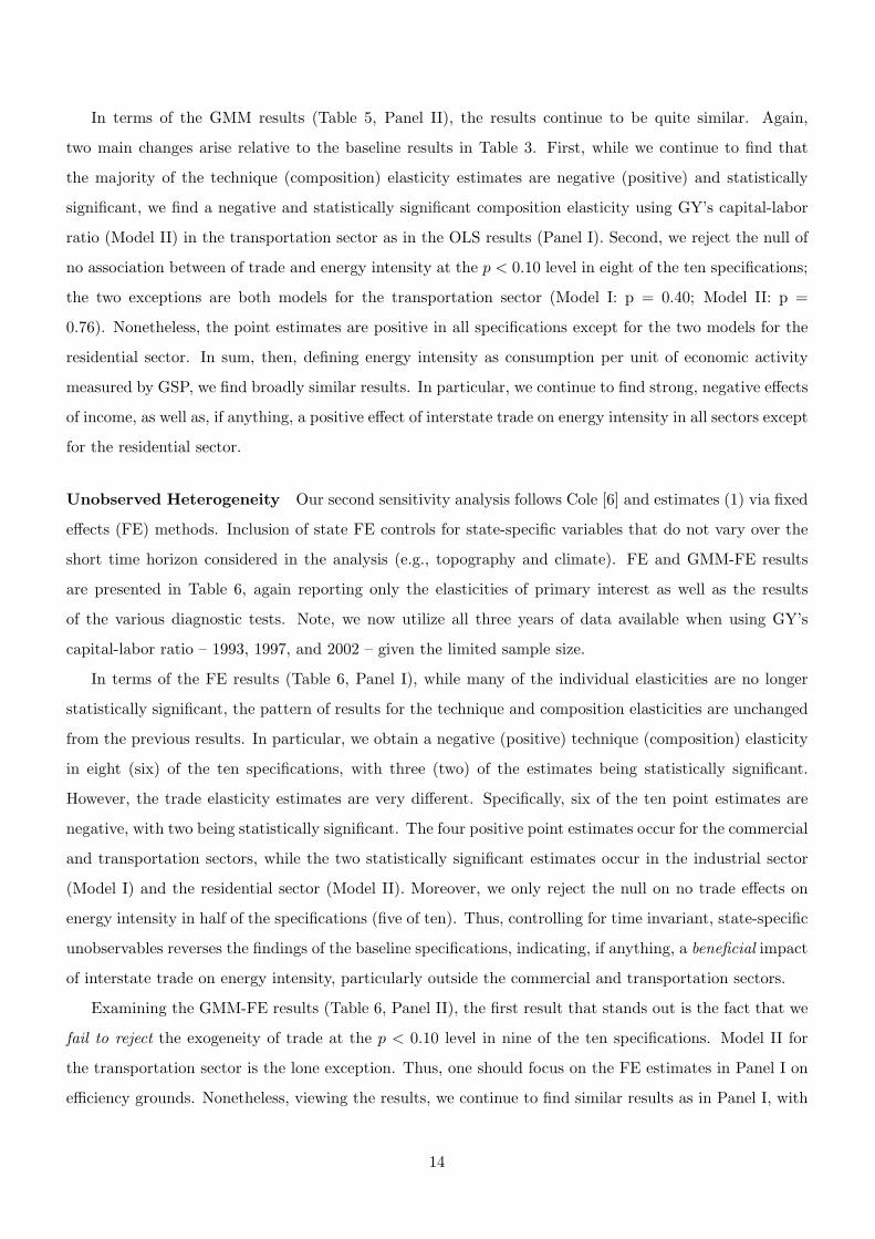
In terms of the GMM results (Table 5, Panel II), the results continue to be quite similar. Again,
two main changes arise relative to the baseline results in Table 3. First, while we continue to find that
the majority of the technique (composition) elasticity estimates are negative (positive) and statistically
significant, we find a negative and statistically significant composition elasticity using GY’s capital-labor
ratio (Model II) in the transportation sector as in the OLS results (Panel I). Second, we reject the null of
no association between of trade and energy intensity at the p < 0.10 level in eight of the ten specifications;
the two exceptions are both models for the transportation sector (Model I: p = 0.40; Model II: p =
0.76). Nonetheless, the point estimates are positive in all specifications except for the two models for the
residential sector. In sum, then, defining energy intensity as consumption per unit of economic activity
measured by GSP, we find broadly similar results. In particular, we continue to find strong, negative effects
of income, as well as, if anything, a positive effect of interstate trade on energy intensity in all sectors except
for the residential sector.
Unobserved Heterogeneity Our second sensitivity analysis follows Cole [6] and estimates (1) via fixed
effects (FE) methods. Inclusion of state FE controls for state-specific variables that do not vary over the
short time horizon considered in the analysis (e.g., topography and climate). FE and GMM-FE results
are presented in Table 6, again reporting only the elasticities of primary interest as well as the results
of the various diagnostic tests. Note, we now utilize all three years of data available when using GY’s
capital-labor ratio – 1993, 1997, and 2002 – given the limited sample size.
In terms of the FE results (Table 6, Panel I), while many of the individual elasticities are no longer
statistically significant, the pattern of results for the technique and composition elasticities are unchanged
from the previous results. In particular, we obtain a negative (positive) technique (composition) elasticity
in eight (six) of the ten specifications, with three (two) of the estimates being statistically significant.
However, the trade elasticity estimates are very different. Specifically, six of the ten point estimates are
negative, with two being statistically significant. The four positive point estimates occur for the commercial
and transportation sectors, while the two statistically significant estimates occur in the industrial sector
(Model I) and the residential sector (Model II). Moreover, we only reject the null on no trade effects on
energy intensity in half of the specifications (five of ten). Thus, controlling for time invariant, state-specific
unobservables reverses the findings of the baseline specifications, indicating, if anything, a beneficial impact
of interstate trade on energy intensity, particularly outside the commercial and transportation sectors.
Examining the GMM-FE results (Table 6, Panel II), the first result that stands out is the fact that we
fail to reject the exogeneity of trade at the p < 0.10 level in nine of the ten specifications. Model II for
the transportation sector is the lone exception. Thus, one should focus on the FE estimates in Panel I on
efficiency grounds. Nonetheless, viewing the results, we continue to find similar results as in Panel I, with
14
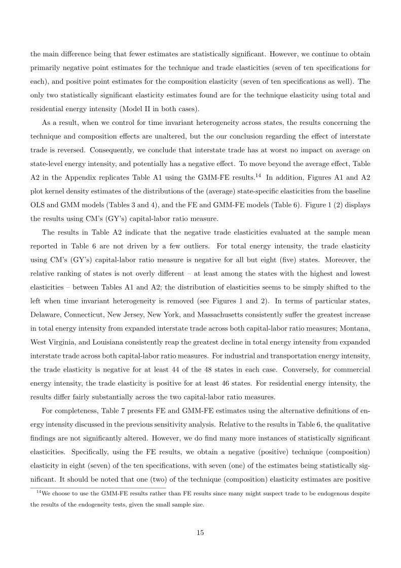
the main difference being that fewer estimates are statistically significant. However, we continue to obtain
primarily negative point estimates for the technique and trade elasticities (seven of ten specifications for
each), and positive point estimates for the composition elasticity (seven of ten specifications as well). The
only two statistically significant elasticity estimates found are for the technique elasticity using total and
residential energy intensity (Model II in both cases).
As a result, when we control for time invariant heterogeneity across states, the results concerning the
technique and composition effects are unaltered, but the our conclusion regarding the effect of interstate
trade is reversed. Consequently, we conclude that interstate trade has at worst no impact on average on
state-level energy intensity, and potentially has a negative effect. To move beyond the average effect, Table
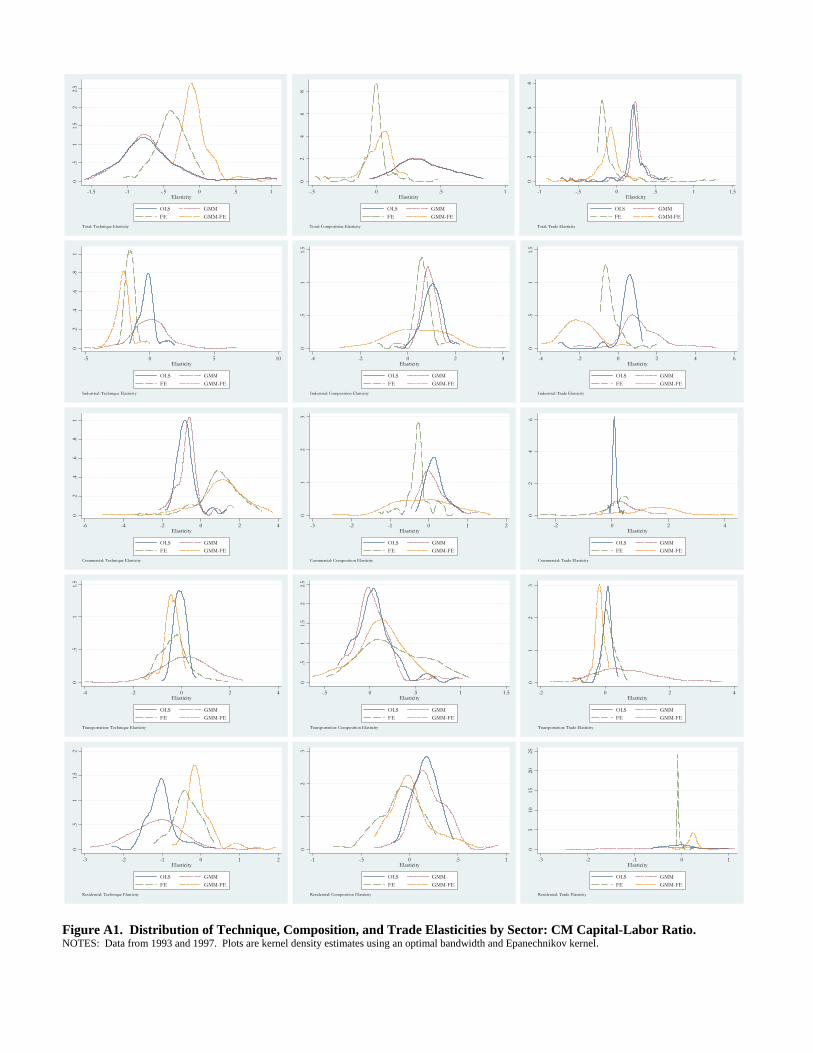
A2 in the Appendix replicates Table A1 using the GMM-FE results.14 In addition, Figures A1 and A2
plot kernel density estimates of the distributions of the (average) state-specific elasticities from the baseline
OLS and GMM models (Tables 3 and 4), and the FE and GMM-FE models (Table 6). Figure 1 (2) displays
the results using CM’s (GY’s) capital-labor ratio measure.
The results in Table A2 indicate that the negative trade elasticities evaluated at the sample mean
reported in Table 6 are not driven by a few outliers. For total energy intensity, the trade elasticity
using CM’s (GY’s) capital-labor ratio measure is negative for all but eight (five) states. Moreover, the
relative ranking of states is not overly different – at least among the states with the highest and lowest
elasticities – between Tables A1 and A2; the distribution of elasticities seems to be simply shifted to the
left when time invariant heterogeneity is removed (see Figures 1 and 2). In terms of particular states,
Delaware, Connecticut, New Jersey, New York, and Massachusetts consistently suffer the greatest increase
in total energy intensity from expanded interstate trade across both capital-labor ratio measures; Montana,
West Virginia, and Louisiana consistently reap the greatest decline in total energy intensity from expanded
interstate trade across both capital-labor ratio measures. For industrial and transportation energy intensity,
the trade elasticity is negative for at least 44 of the 48 states in each case. Conversely, for commercial
energy intensity, the trade elasticity is positive for at least 46 states. For residential energy intensity, the
results differ fairly substantially across the two capital-labor ratio measures.
For completeness, Table 7 presents FE and GMM-FE estimates using the alternative definitions of en-
ergy intensity discussed in the previous sensitivity analysis. Relative to the results in Table 6, the qualitative
findings are not significantly altered. However, we do find many more instances of statistically significant
elasticities. Specifically, using the FE results, we obtain a negative (positive) technique (composition)
elasticity in eight (seven) of the ten specifications, with seven (one) of the estimates being statistically sig-
nificant. It should be noted that one (two) of the technique (composition) elasticity estimates are positive14We choose to use the GMM-FE results rather than FE results since many might suspect trade to be endogenous despite
the results of the endogeneity tests, given the small sample size.
15

(negative) and statistically significant as well. In addition, the trade elasticity estimates are negative in
seven specifications, and statistically significant in two (Model I for the transportation sector and Model
II for the residential sector). Finally, we reject the null of no trade effects on energy intensity in only
four of the ten specifications. Examination of the GMM-FE results also yields quite similar conclusions to
those gained from Table 6. First, we fail to reject the null of exogeneity of trade in all ten specifications
at the p < 0.10 level. Second, we obtain a negative (positive) technique (composition) elasticity in eight
(seven) of the ten specifications, with five (none) of the estimates being statistically significant; one of the
composition elasticities is negative and statistically significant (Model II for the transportation sector).
Moreover, the trade elasticity estimates are negative in seven specifications, and statistically significant in
two (Model II for total energy intensity and Model II for the transportation sector). Finally, we reject
the null of no trade effects on energy intensity at the p < 0.10 level in but one specification. Thus, using
our alternative definitions for energy intensity and does not alter the conclusions from the previous models
controlling for time invariant, state-specific heterogeneity.
Per Capita Energy Consumption As a final sensitivity analysis, we follow Stern [25] and Cole [6] and
assess the impact of interstate trade on per capita energy consumption, rather than energy intensity. As
noted in Cole [6], when the dependent variable is measured in per capita terms, the elasticity with respect
to per capita GSP captures both scale and technique effects. The results are reported in Tables 8 and
9, with Table 8 providing the results obtained using OLS and GMM and Table 9 reporting the FE and
GMM-FE results. In general, the implications from the preceding results are unaltered.
In Table 8, we obtain a negative combined scale and technique elasticity in seven of ten specifications
using either OLS (Panel I) or GMM (Panel II), with three of the seven being statistically significant in
both cases. One estimate is positive and statistically significant in each panel (Model I for commercial
energy consumption per capita). Thus, the negative technique effect tends to dominate the scale effect.
In addition, the composition (trade) elasticity estimate is positive in nine (seven) of ten specifications in
Panels I and II of Table 8. The composition elasticity is positive (negative) and statistically significant in
five (one) specifications in each panel, whereas the trade elasticity is positive (negative) and statistically
significant in four (one) specification in Panel II; the trade elasticity is always statistically insignificant
in Panel I. Finally, according to the GMM estimates, we reject the null of no trade effects in nine of ten
specifications, and we reject the null of trade being exogenous in six cases. As a result, the OLS and GMM
per capita results largely confirm the previous results based on energy intensity reported in Tables 3 and
4.
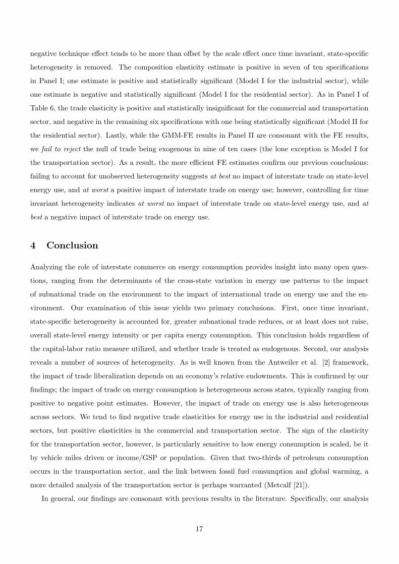
In Table 9, we obtain a positive combined scale and technique elasticity in seven of ten specifications
using FE (Panel I), with one being statistically significant (Model I for the commercial sector). Thus, the
16
negative technique effect tends to be more than offset by the scale effect once time invariant, state-specific
heterogeneity is removed. The composition elasticity estimate is positive in seven of ten specifications
in Panel I; one estimate is positive and statistically significant (Model I for the industrial sector), while
one estimate is negative and statistically significant (Model I for the residential sector). As in Panel I of
Table 6, the trade elasticity is positive and statistically insignificant for the commercial and transportation
sector, and negative in the remaining six specifications with one being statistically significant (Model II for
the residential sector). Lastly, while the GMM-FE results in Panel II are consonant with the FE results,
we fail to reject the null of trade being exogenous in nine of ten cases (the lone exception is Model I for
the transportation sector). As a result, the more efficient FE estimates confirm our previous conclusions:
failing to account for unobserved heterogeneity suggests at best no impact of interstate trade on state-level
energy use, and at worst a positive impact of interstate trade on energy use; however, controlling for time
invariant heterogeneity indicates at worst no impact of interstate trade on state-level energy use, and at
best a negative impact of interstate trade on energy use.
4 Conclusion
Analyzing the role of interstate commerce on energy consumption provides insight into many open ques-
tions, ranging from the determinants of the cross-state variation in energy use patterns to the impact
of subnational trade on the environment to the impact of international trade on energy use and the en-
vironment. Our examination of this issue yields two primary conclusions. First, once time invariant,
state-specific heterogeneity is accounted for, greater subnational trade reduces, or at least does not raise,
overall state-level energy intensity or per capita energy consumption. This conclusion holds regardless of
the capital-labor ratio measure utilized, and whether trade is treated as endogenous. Second, our analysis
reveals a number of sources of heterogeneity. As is well known from the Antweiler et al. [2] framework,
the impact of trade liberalization depends on an economy’s relative endowments. This is confirmed by our
findings; the impact of trade on energy consumption is heterogeneous across states, typically ranging from
positive to negative point estimates. However, the impact of trade on energy use is also heterogeneous
across sectors. We tend to find negative trade elasticities for energy use in the industrial and residential
sectors, but positive elasticities in the commercial and transportation sector. The sign of the elasticity
for the transportation sector, however, is particularly sensitive to how energy consumption is scaled, be it
by vehicle miles driven or income/GSP or population. Given that two-thirds of petroleum consumption
occurs in the transportation sector, and the link between fossil fuel consumption and global warming, a
more detailed analysis of the transportation sector is perhaps warranted (Metcalf [21]).
In general, our findings are consonant with previous results in the literature. Specifically, our analysis
17
provides further evidence against a harmful environmental effect of expanded trade, as documented in,
among others, Antweiler et al. [2], Harbaugh et al. [14], Frankel and Rose [12], and Stern [25] using
cross-country data and Chintrakarn and Millimet [4] using subnational data. Our findings also confirm the
role of economic factors in explaining at least a portion of the cross-state variation in energy use in the
US, as discussed in Metcalf [20]. However, our results do contrast starkly with those in Cole [6]. Thus,
assuming this discrepancy is not driven by inconsistencies that may arise in cross-country panel data, what
accounts for the differential impact of cross-country trade on country-level energy intensity, as opposed to
interstate trade on state-level energy intensity, is an open question, deserving attention.
18
References
[1] J.E. Anderson and E. van Wincoop, Gravity with gravitas: a solution to the border puzzle, Amer.
Econom. Rev. 93, 170-192 (2003).
[2] W. Antweiler, B.R. Copeland, and M.S. Taylor, Is free trade good for the environment?, Amer.
Econom. Rev. 91, 877-908 (2001).
[3] M. Bernstein, K. Fonkych, S. Loeb, and D. Loughran, State-level changes in energy intensity and their
national implications, Santa Monica, CA: Rand (2003).
[4] P. Chintrakarn and D.L. Millimet, The environmental consequences of trade: evidence from subna-
tional trade flows, J. Environ. Econom. Management 52, 430-453 (2006).
[5] J.P. Cohen and C.J. Morrison Paul, Public infrastructure investment, costs, and inter-state spatial
spillovers in U.S. Manufacturing: 1982-96, Rev. of Econom. Statist. 86, 551-560 (2004).
[6] M.A. Cole, Does trade liberalization increase national energy use?, Econom. Letters 92, 108-112 (2006).
[7] P.-P. Combes, M. Lafourcade, and T. Mayer, The trade-creating effects of business and social networks:
evidence from France, J. Internat. Econom. 66, 1-29 (2005).
[8] B.R. Copeland and M.S. Taylor, Trade, growth, and the environment, J. Econom. Lit. 42, 7-71 (2004).
[9] J.M. Dean, Testing the impact of trade liberalization on the environment: theory and evidence,
Canadian J. of Econom. 35, 819-842 (2002).
[10] J. Ederington and J. Minier, Is environmental policy a secondary trade barrier? an empirical analysis,
Canad. J. of Econom. 36, 137-154 (2003).
[11] P.G. Fredriksson, H.R.J. Vollebergh, and E. Dijkgraaf, Corruption and energy efficiency in OECD
countries: theory and evidence, J. Environ. Econom. Management 47, 207-231 (2004).
[12] J.A. Frankel and A.K. Rose, Is trade good or bad for the environment? sorting out the causality, Rev.
Econom. Statist. 87, 85-91 (2005).
[13] G.A. Garofalo and S. Yamarik, Regional convergence: evidence from a new state-by-state capital stock
series, Rev. Econom. Statist. 84, 316-323 (2002).
[14] W.T. Harbaugh, A. Levinson, and D.M. Wilson, Reexamining the empirical evidence for an environ-
mental kuznets curve, Rev. Econom. Statist. 84, 541-551 (2002).
19
[15] A.R. Hall, G.D. Rudebusch, and D.W. Wilcox, Judging instrument relevance in instrumental variables
estimation, Internat. Econom. Rev. 37, 283-298 (1996).
[16] D.J. Henderson and D.L. Millimet, Is gravity linear?, J. Applied Econometrics (forthcoming).
[17] R. Hillberry and D. Hummels, Intra-national home bias: some explanations, Rev. Econom. Statist.
85, 1089-1092 (2003).
[18] ICTSD, Linking trade, climate change and energy, ICTSD Trade and Sustainable Energy Series,
International Centre for Trade and Sustainable Development, Geneva, Switzerland (2006).
[19] T. Knaap, Trade, location, and wages in the United States, Reg. Sci. Urb. Econom. 36, 595-612 (2006).
[20] G.E. Metcalf, Energy Conservation in the United States: understanding its role in climate policy,
NBER WP 12272 (2006).
[21] G.E. Metcalf, Federal tax policy towards energy, NBER WP 12568 (2006).
[22] D.L. Millimet and T. Osang, Do state borders matter for US intranational trade? the role of history
and internal migration, Canad. J. Econom. (forthcoming).
[23] C.J. Morrison Paul and A.E. Schwartz, State infrastructure and productive performance, Amer.
Econom. Rev. 86, 1095-1111 (1996).
[24] J.M.C. Santos Silva and S. Tenreyro, The log of gravity, Rev. of Econom. Statist. (forthcoming).
[25] D.I. Stern, The effect of NAFTA on energy and environmental efficiency in Mexico, Policy Studies J.,
(forthcoming).
[26] M.S. Taylor, Unbundling the pollution haven hypothesis, Adv. Econom. Anal. Policy 4 (2), Article 8
(2004).
[27] US Energy Information Administration, Annual energy review 2004, Washington, D.C.: Department
of Energy (2005).
[28] H.C. Wolf, Intranational home bias in trade, Rev. Econom. Statist. 82, 555-63 (2000).
20

Table A1. Average Trade Elasticities by State: GMMState
Est. Rk. Est. Rk. Est. Rk. Est. Rk. Est. Rk. Est. Rk. Est. Rk. Est. Rk. Est. Rk. Est. Rk.
DE 0.723 (1) 1.138 (5) 2.231 (6) 4.437 (5) 0.410 (21) 1.220 (9) -0.242 (41) 0.297 (38) 0.898 (3) 1.222 (5)CT 0.632 (2) 1.553 (3) 1.938 (10) 4.307 (6) 0.050 (39) 2.089 (3) -0.247 (43) 0.651 (28) 1.096 (1) 1.660 (3)MS 0.512 (3) 0.211 (22) 4.904 (1) 4.988 (2) 1.887 (1) 1.091 (10) 3.508 (1) 3.835 (1) -2.368 (48) -1.900 (47)NJ 0.464 (4) 1.371 (4) 1.083 (19) 2.872 (12) -0.050 (43) 1.936 (4) -0.297 (45) 0.528 (32) 0.910 (2) 1.475 (4)NY 0.432 (5) 2.563 (2) 0.843 (27) 4.937 (3) 0.080 (37) 4.058 (2) -0.329 (46) 1.981 (10) 0.738 (5) 2.560 (2)MA 0.393 (6) 0.534 (10) 0.820 (30) 1.399 (22) -0.115 (44) 0.437 (17) -0.242 (42) -0.127 (48) 0.826 (4) 0.594 (6)AR 0.391 (7) 0.040 (33) 3.381 (4) 3.035 (10) 1.342 (4) 0.560 (15) 2.539 (4) 2.622 (6) -1.683 (45) -1.523 (45)NV 0.351 (8) 0.457 (13) 0.685 (34) 1.639 (19) -0.125 (46) 0.220 (25) -0.179 (40) 0.157 (41) 0.735 (6) 0.401 (9)OK 0.323 (9) -0.294 (48) 2.615 (5) 0.370 (42) 1.117 (6) 0.189 (27) 2.041 (5) 1.142 (18) -1.384 (43) -1.408 (44)MT 0.308 (10) -0.113 (43) 3.474 (3) 3.001 (11) 1.607 (3) 0.491 (16) 2.682 (3) 2.669 (5) -2.065 (46) -1.830 (46)IL 0.301 (11) 0.513 (11) 0.416 (39) 0.608 (34) 0.091 (36) 0.641 (13) -0.140 (39) -0.056 (44) 0.422 (9) 0.505 (8)CA 0.300 (12) 0.397 (16) 0.467 (38) 0.479 (40) 0.068 (38) 0.433 (18) -0.085 (38) -0.104 (47) 0.418 (10) 0.362 (10)AZ 0.297 (13) -0.141 (44) 1.872 (12) 0.766 (31) 0.645 (15) -0.002 (41) 1.443 (12) 1.075 (19) -0.759 (34) -1.020 (38)WV 0.295 (14) -0.229 (47) 3.834 (2) 1.654 (18) 1.762 (2) 0.793 (12) 2.937 (2) 2.124 (9) -2.302 (47) -1.914 (48)FL 0.293 (15) 0.058 (29) 1.778 (14) 1.489 (21) 0.564 (16) 0.198 (26) 1.357 (13) 1.419 (15) -0.655 (33) -0.841 (37)UT 0.288 (16) -0.102 (42) 1.968 (9) 1.182 (24) 0.805 (12) 0.088 (31) 1.556 (8) 1.355 (16) -0.961 (37) -1.093 (41)MN 0.278 (17) 0.184 (24) 0.606 (37) 0.452 (41) -0.040 (42) 0.037 (38) 0.120 (34) 0.044 (43) 0.402 (11) 0.015 (15)SD 0.274 (18) 0.877 (7) 1.880 (11) 4.137 (8) -0.007 (41) 1.250 (8) 1.288 (14) 2.799 (4) -0.091 (18) -0.154 (18)ID 0.261 (19) -0.216 (46) 2.160 (7) 1.119 (25) 1.036 (8) 0.053 (35) 1.763 (7) 1.432 (14) -1.284 (41) -1.342 (43)NH 0.259 (20) 0.447 (14) 0.828 (29) 1.885 (16) -0.219 (48) 0.340 (19) 0.315 (31) 0.945 (24) 0.473 (7) 0.056 (13)MO 0.256 (21) -0.002 (35) 1.064 (20) 0.504 (38) 0.290 (28) -0.034 (47) 0.762 (19) 0.608 (30) -0.216 (23) -0.542 (30)WI 0.255 (22) 0.114 (27) 0.973 (24) 0.921 (28) 0.226 (33) 0.062 (34) 0.664 (25) 0.761 (26) -0.117 (20) -0.412 (24)MI 0.255 (23) -0.062 (40) 1.014 (21) -0.134 (46) 0.284 (29) -0.031 (46) 0.718 (21) 0.270 (39) -0.195 (21) -0.513 (28)OR 0.250 (24) 0.012 (34) 0.986 (23) 0.560 (37) 0.353 (24) -0.022 (45) 0.717 (22) 0.617 (29) -0.266 (27) -0.524 (29)NE 0.248 (25) 0.133 (26) 0.627 (36) 0.613 (33) 0.189 (35) 0.023 (39) 0.341 (30) 0.393 (35) 0.038 (16) -0.215 (20)RI 0.246 (26) 0.288 (17) 1.351 (18) 1.691 (17) -0.204 (47) 0.301 (22) 0.840 (17) 1.225 (17) 0.232 (12) -0.344 (23)WA 0.242 (27) 0.199 (23) 0.270 (43) 0.227 (43) 0.234 (32) 0.126 (30) -0.024 (37) -0.064 (46) 0.143 (13) 0.066 (12)PA 0.240 (28) -0.039 (38) 0.838 (28) -0.177 (47) 0.335 (26) -0.005 (42) 0.609 (26) 0.214 (40) -0.221 (24) -0.451 (26)KS 0.238 (29) -0.028 (36) 1.003 (22) 0.496 (39) 0.440 (20) -0.038 (48) 0.786 (18) 0.657 (27) -0.394 (28) -0.611 (33)CO 0.237 (30) 0.265 (19) 0.287 (42) 0.096 (44) 0.219 (34) 0.316 (20) 0.010 (35) -0.059 (45) 0.137 (14) 0.140 (11)OH 0.233 (31) 0.052 (31) 0.739 (33) 0.563 (36) 0.340 (25) -0.018 (44) 0.534 (27) 0.536 (31) -0.206 (22) -0.413 (25)VA 0.233 (32) 0.251 (20) 0.239 (44) 0.951 (26) 0.255 (31) 0.072 (32) -0.015 (36) 0.314 (37) 0.105 (15) 0.019 (14)IA 0.229 (33) 0.498 (12) 0.934 (25) 2.562 (13) 0.478 (19) 0.614 (14) 0.752 (20) 1.763 (13) -0.429 (29) -0.260 (22)MD 0.228 (34) 0.213 (21) 0.384 (41) 0.939 (27) 0.261 (30) 0.067 (33) 0.162 (33) 0.462 (34) 0.018 (17) -0.107 (17)ND 0.227 (35) 0.055 (30) 1.786 (13) 1.962 (15) 0.966 (9) 0.315 (21) 1.518 (9) 1.817 (12) -1.173 (40) -1.056 (39)AL 0.225 (36) -0.065 (41) 2.158 (8) 1.974 (14) 1.157 (5) 0.274 (23) 1.812 (6) 1.931 (11) -1.454 (44) -1.331 (42)NC 0.222 (37) 0.285 (18) 0.654 (35) 1.534 (20) 0.367 (23) 0.245 (24) 0.485 (28) 1.039 (20) -0.226 (25) -0.257 (21)GA 0.216 (38) 0.065 (28) 0.414 (40) -0.068 (45) 0.324 (27) 0.044 (37) 0.251 (32) 0.064 (42) -0.099 (19) -0.209 (19)SC 0.206 (39) 0.447 (15) 1.660 (15) 3.309 (9) 0.961 (10) 0.828 (11) 1.447 (11) 2.545 (7) -1.168 (39) -0.759 (35)KY 0.197 (40) -0.175 (45) 1.411 (17) 0.643 (32) 0.860 (11) -0.017 (43) 1.255 (15) 1.033 (21) -1.015 (38) -1.064 (40)IN 0.196 (41) 0.048 (32) 0.793 (31) 0.887 (29) 0.552 (17) 0.048 (36) 0.704 (23) 0.874 (25) -0.522 (32) -0.581 (32)TN 0.196 (42) 0.139 (25) 0.754 (32) 1.219 (23) 0.535 (18) 0.144 (29) 0.667 (24) 1.030 (22) -0.492 (31) -0.502 (27)NM 0.140 (43) -0.060 (39) 0.880 (26) 0.812 (30) 0.745 (13) 0.020 (40) 0.890 (16) 1.000 (23) -0.842 (36) -0.836 (36)ME 0.137 (44) 0.735 (9) 1.639 (16) 4.526 (4) 1.066 (7) 1.303 (6) 1.506 (10) 3.286 (2) -1.363 (42) -0.662 (34)TX 0.001 (45) 0.748 (8) -0.544 (46) 0.590 (35) 0.398 (22) 1.350 (5) -0.259 (44) 0.517 (33) -0.227 (26) 0.543 (7)VT -0.063 (46) 0.919 (6) 0.073 (45) 4.231 (7) 0.651 (14) 1.291 (7) 0.449 (29) 2.821 (3) -0.820 (35) -0.096 (16)WY -0.389 (47) 2.859 (1) -2.073 (48) 5.291 (1) -0.116 (45) 4.645 (1) -1.632 (48) 2.469 (8) 0.436 (8) 2.777 (1)LA -0.597 (48) -0.035 (37) -1.740 (47) -0.295 (48) 0.020 (40) 0.179 (28) -0.575 (47) 0.339 (36) -0.436 (30) -0.546 (31)
NOTES: Averages computed over 1993 and 1997.
CMTotal Industrial Commerical Transportation
GYResidential
CM GY CM GY CM GY CM GY
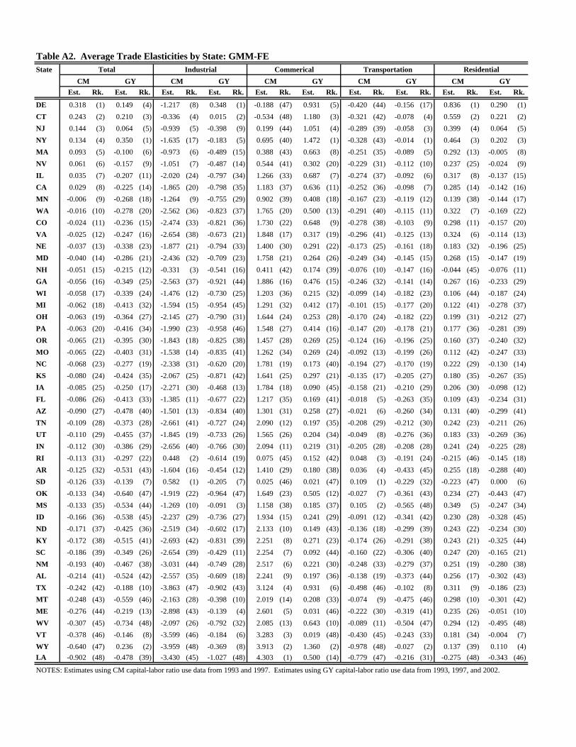
Table A2. Average Trade Elasticities by State: GMM-FEState
Est. Rk. Est. Rk. Est. Rk. Est. Rk. Est. Rk. Est. Rk. Est. Rk. Est. Rk. Est. Rk. Est. Rk.
DE 0.318 (1) 0.149 (4) -1.217 (8) 0.348 (1) -0.188 (47) 0.931 (5) -0.420 (44) -0.156 (17) 0.836 (1) 0.290 (1)CT 0.243 (2) 0.210 (3) -0.336 (4) 0.015 (2) -0.534 (48) 1.180 (3) -0.321 (42) -0.078 (4) 0.559 (2) 0.221 (2)NJ 0.144 (3) 0.064 (5) -0.939 (5) -0.398 (9) 0.199 (44) 1.051 (4) -0.289 (39) -0.058 (3) 0.399 (4) 0.064 (5)NY 0.134 (4) 0.350 (1) -1.635 (17) -0.183 (5) 0.695 (40) 1.472 (1) -0.328 (43) -0.014 (1) 0.464 (3) 0.202 (3)MA 0.093 (5) -0.100 (6) -0.973 (6) -0.489 (15) 0.388 (43) 0.663 (8) -0.251 (35) -0.089 (5) 0.292 (13) -0.005 (8)NV 0.061 (6) -0.157 (9) -1.051 (7) -0.487 (14) 0.544 (41) 0.302 (20) -0.229 (31) -0.112 (10) 0.237 (25) -0.024 (9)IL 0.035 (7) -0.207 (11) -2.020 (24) -0.797 (34) 1.266 (33) 0.687 (7) -0.274 (37) -0.092 (6) 0.317 (8) -0.137 (15)CA 0.029 (8) -0.225 (14) -1.865 (20) -0.798 (35) 1.183 (37) 0.636 (11) -0.252 (36) -0.098 (7) 0.285 (14) -0.142 (16)MN -0.006 (9) -0.268 (18) -1.264 (9) -0.755 (29) 0.902 (39) 0.408 (18) -0.167 (23) -0.119 (12) 0.139 (38) -0.144 (17)WA -0.016 (10) -0.278 (20) -2.562 (36) -0.823 (37) 1.765 (20) 0.500 (13) -0.291 (40) -0.115 (11) 0.322 (7) -0.169 (22)CO -0.024 (11) -0.236 (15) -2.474 (33) -0.821 (36) 1.730 (22) 0.648 (9) -0.278 (38) -0.103 (9) 0.298 (11) -0.157 (20)VA -0.025 (12) -0.247 (16) -2.654 (38) -0.673 (21) 1.848 (17) 0.317 (19) -0.296 (41) -0.125 (13) 0.324 (6) -0.114 (13)NE -0.037 (13) -0.338 (23) -1.877 (21) -0.794 (33) 1.400 (30) 0.291 (22) -0.173 (25) -0.161 (18) 0.183 (32) -0.196 (25)MD -0.040 (14) -0.286 (21) -2.436 (32) -0.709 (23) 1.758 (21) 0.264 (26) -0.249 (34) -0.145 (15) 0.268 (15) -0.147 (19)NH -0.051 (15) -0.215 (12) -0.331 (3) -0.541 (16) 0.411 (42) 0.174 (39) -0.076 (10) -0.147 (16) -0.044 (45) -0.076 (11)GA -0.056 (16) -0.349 (25) -2.563 (37) -0.921 (44) 1.886 (16) 0.476 (15) -0.246 (32) -0.141 (14) 0.267 (16) -0.233 (29)WI -0.058 (17) -0.339 (24) -1.476 (12) -0.730 (25) 1.203 (36) 0.215 (32) -0.099 (14) -0.182 (23) 0.106 (44) -0.187 (24)MI -0.062 (18) -0.413 (32) -1.594 (15) -0.954 (45) 1.291 (32) 0.412 (17) -0.101 (15) -0.177 (20) 0.122 (41) -0.278 (37)OH -0.063 (19) -0.364 (27) -2.145 (27) -0.790 (31) 1.644 (24) 0.253 (28) -0.170 (24) -0.182 (22) 0.199 (31) -0.212 (27)PA -0.063 (20) -0.416 (34) -1.990 (23) -0.958 (46) 1.548 (27) 0.414 (16) -0.147 (20) -0.178 (21) 0.177 (36) -0.281 (39)OR -0.065 (21) -0.395 (30) -1.843 (18) -0.825 (38) 1.457 (28) 0.269 (25) -0.124 (16) -0.196 (25) 0.160 (37) -0.240 (32)MO -0.065 (22) -0.403 (31) -1.538 (14) -0.835 (41) 1.262 (34) 0.269 (24) -0.092 (13) -0.199 (26) 0.112 (42) -0.247 (33)NC -0.068 (23) -0.277 (19) -2.338 (31) -0.620 (20) 1.781 (19) 0.173 (40) -0.194 (27) -0.170 (19) 0.222 (29) -0.130 (14)KS -0.080 (24) -0.424 (35) -2.067 (25) -0.871 (42) 1.641 (25) 0.297 (21) -0.135 (17) -0.205 (27) 0.180 (35) -0.267 (35)IA -0.085 (25) -0.250 (17) -2.271 (30) -0.468 (13) 1.784 (18) 0.090 (45) -0.158 (21) -0.210 (29) 0.206 (30) -0.098 (12)FL -0.086 (26) -0.413 (33) -1.385 (11) -0.677 (22) 1.217 (35) 0.169 (41) -0.018 (5) -0.263 (35) 0.109 (43) -0.234 (31)AZ -0.090 (27) -0.478 (40) -1.501 (13) -0.834 (40) 1.301 (31) 0.258 (27) -0.021 (6) -0.260 (34) 0.131 (40) -0.299 (41)TN -0.109 (28) -0.373 (28) -2.661 (41) -0.727 (24) 2.090 (12) 0.197 (35) -0.208 (29) -0.212 (30) 0.242 (23) -0.211 (26)UT -0.110 (29) -0.455 (37) -1.845 (19) -0.733 (26) 1.565 (26) 0.204 (34) -0.049 (8) -0.276 (36) 0.183 (33) -0.269 (36)IN -0.112 (30) -0.386 (29) -2.656 (40) -0.766 (30) 2.094 (11) 0.219 (31) -0.205 (28) -0.208 (28) 0.241 (24) -0.225 (28)RI -0.113 (31) -0.297 (22) 0.448 (2) -0.614 (19) 0.075 (45) 0.152 (42) 0.048 (3) -0.191 (24) -0.215 (46) -0.145 (18)AR -0.125 (32) -0.531 (43) -1.604 (16) -0.454 (12) 1.410 (29) 0.180 (38) 0.036 (4) -0.433 (45) 0.255 (18) -0.288 (40)SD -0.126 (33) -0.139 (7) 0.582 (1) -0.205 (7) 0.025 (46) 0.021 (47) 0.109 (1) -0.229 (32) -0.223 (47) 0.000 (6)OK -0.133 (34) -0.640 (47) -1.919 (22) -0.964 (47) 1.649 (23) 0.505 (12) -0.027 (7) -0.361 (43) 0.234 (27) -0.443 (47)MS -0.133 (35) -0.534 (44) -1.269 (10) -0.091 (3) 1.158 (38) 0.185 (37) 0.105 (2) -0.565 (48) 0.349 (5) -0.247 (34)ID -0.166 (36) -0.538 (45) -2.237 (29) -0.736 (27) 1.934 (15) 0.241 (29) -0.091 (12) -0.341 (42) 0.230 (28) -0.328 (45)ND -0.171 (37) -0.425 (36) -2.519 (34) -0.602 (17) 2.133 (10) 0.149 (43) -0.136 (18) -0.299 (39) 0.243 (22) -0.234 (30)KY -0.172 (38) -0.515 (41) -2.693 (42) -0.831 (39) 2.251 (8) 0.271 (23) -0.174 (26) -0.291 (38) 0.243 (21) -0.325 (44)SC -0.186 (39) -0.349 (26) -2.654 (39) -0.429 (11) 2.254 (7) 0.092 (44) -0.160 (22) -0.306 (40) 0.247 (20) -0.165 (21)NM -0.193 (40) -0.467 (38) -3.031 (44) -0.749 (28) 2.517 (6) 0.221 (30) -0.248 (33) -0.279 (37) 0.251 (19) -0.280 (38)AL -0.214 (41) -0.524 (42) -2.557 (35) -0.609 (18) 2.241 (9) 0.197 (36) -0.138 (19) -0.373 (44) 0.256 (17) -0.302 (43)TX -0.242 (42) -0.188 (10) -3.863 (47) -0.902 (43) 3.124 (4) 0.931 (6) -0.498 (46) -0.102 (8) 0.311 (9) -0.186 (23)MT -0.248 (43) -0.559 (46) -2.163 (28) -0.398 (10) 2.019 (14) 0.208 (33) -0.074 (9) -0.475 (46) 0.298 (10) -0.301 (42)ME -0.276 (44) -0.219 (13) -2.898 (43) -0.139 (4) 2.601 (5) 0.031 (46) -0.222 (30) -0.319 (41) 0.235 (26) -0.051 (10)WV -0.307 (45) -0.734 (48) -2.097 (26) -0.792 (32) 2.085 (13) 0.643 (10) -0.089 (11) -0.504 (47) 0.294 (12) -0.495 (48)VT -0.378 (46) -0.146 (8) -3.599 (46) -0.184 (6) 3.283 (3) 0.019 (48) -0.430 (45) -0.243 (33) 0.181 (34) -0.004 (7)WY -0.640 (47) 0.236 (2) -3.959 (48) -0.369 (8) 3.913 (2) 1.360 (2) -0.978 (48) -0.027 (2) 0.137 (39) 0.110 (4)LA -0.902 (48) -0.478 (39) -3.430 (45) -1.027 (48) 4.303 (1) 0.500 (14) -0.779 (47) -0.216 (31) -0.275 (48) -0.343 (46)
NOTES: Estimates using CM capital-labor ratio use data from 1993 and 1997. Estimates using GY capital-labor ratio use data from 1993, 1997, and 2002.
CMTotal Industrial Commerical Transportation
GYResidential
CM GY CM GY CM GY CM GY
0.5
11.
52
2.5
-1.5 -1 -.5 0 .5 1Elasticity
OLS GMMFE GMM-FE
Total: Technique Elasticity
02
46
8
-.5 0 .5 1Elasticity
OLS GMMFE GMM-FE
Total: Composition Elasticity
02
46
8
-1 -.5 0 .5 1 1.5Elasticity
OLS GMMFE GMM-FE
Total: Trade Elasticity
0.2
.4.6
.81
-5 0 5 10Elasticity
OLS GMMFE GMM-FE
Industrial: Technique Elasticity
0.5
11.
5
-4 -2 0 2 4Elasticity
OLS GMMFE GMM-FE
Industrial: Composition Elasticity
0.5
11.
5
-4 -2 0 2 4 6Elasticity
OLS GMMFE GMM-FE
Industrial: Trade Elasticity
0.2
.4.6
.81
-6 -4 -2 0 2 4Elasticity
OLS GMMFE GMM-FE
Commercial: Technique Elasticity
01
23
-3 -2 -1 0 1 2Elasticity
OLS GMMFE GMM-FE
Commercial: Composition Elasticity
02
46
-2 0 2 4Elasticity
OLS GMMFE GMM-FE
Commercial: Trade Elasticity
0.5
11.
5
-4 -2 0 2 4Elasticity
OLS GMMFE GMM-FE
Transportation: Technique Elasticity
0.5
11.
52
2.5
-.5 0 .5 1 1.5Elasticity
OLS GMMFE GMM-FE
Transportation: Composition Elasticity
01
23
-2 0 2 4Elasticity
OLS GMMFE GMM-FE
Transportation: Trade Elasticity
0.5
11.
52
-3 -2 -1 0 1 2Elasticity
OLS GMMFE GMM-FE
Residential: Technique Elasticity
01
23
-1 -.5 0 .5 1Elasticity
OLS GMMFE GMM-FE
Residential: Composition Elasticity
05
1015
2025
-3 -2 -1 0 1Elasticity
OLS GMMFE GMM-FE
Residential: Trade Elasticity
Figure A1. Distribution of Technique, Composition, and Trade Elasticities by Sector: CM Capital-Labor Ratio. NOTES: Data from 1993 and 1997. Plots are kernel density estimates using an optimal bandwidth and Epanechnikov kernel.
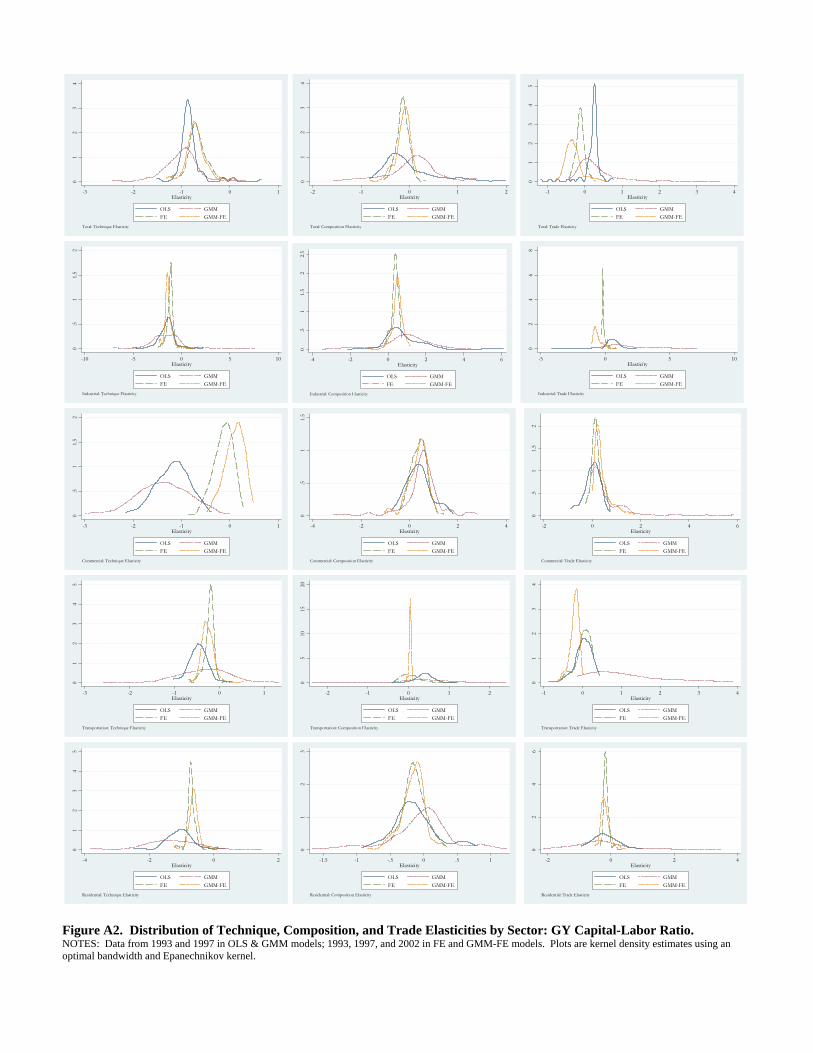
01
23
4
-3 -2 -1 0 1Elasticity
OLS GMMFE GMM-FE
Total: Technique Elasticity
01
23
4
-2 -1 0 1 2Elasticity
OLS GMMFE GMM-FE
Total: Composition Elasticity
01
23
45
-1 0 1 2 3 4Elasticity
OLS GMMFE GMM-FE
Total: Trade Elasticity
0.5
11.
52
-10 -5 0 5 10Elasticity
OLS GMMFE GMM-FE
Industrial: Technique Elasticity
0.5
11.
52
2.5
-4 -2 0 2 4 6Elasticity
OLS GMMFE GMM-FE
Industrial: Composition Elasticity
02
46
8
-5 0 5 10Elasticity
OLS GMMFE GMM-FE
Industrial: Trade Elasticity
0.5
11.
52
-3 -2 -1 0 1Elasticity
OLS GMMFE GMM-FE
Commercial: Technique Elasticity
0.5
11.
5
-4 -2 0 2 4Elasticity
OLS GMMFE GMM-FE
Commercial: Composition Elasticity
0.5
11.
52
-2 0 2 4 6Elasticity
OLS GMMFE GMM-FE
Commercial: Trade Elasticity
01
23
45
-3 -2 -1 0 1Elasticity
OLS GMMFE GMM-FE
Transportation: Technique Elasticity
05
1015
20
-2 -1 0 1 2Elasticity
OLS GMMFE GMM-FE
Transportation: Composition Elasticity
01
23
4
-1 0 1 2 3 4Elasticity
OLS GMMFE GMM-FE
Transportation: Trade Elasticity
01
23
45
-4 -2 0 2Elasticity
OLS GMMFE GMM-FE
Residential: Technique Elasticity
01
23
-1.5 -1 -.5 0 .5 1Elasticity
OLS GMMFE GMM-FE
Residential: Composition Elasticity
02
46
-2 0 2 4Elasticity
OLS GMMFE GMM-FE
Residential: Trade Elasticity
Figure A2. Distribution of Technique, Composition, and Trade Elasticities by Sector: GY Capital-Labor Ratio. NOTES: Data from 1993 and 1997 in OLS & GMM models; 1993, 1997, and 2002 in FE and GMM-FE models. Plots are kernel density estimates using an optimal bandwidth and Epanechnikov kernel.

Table 1. Summary StatisticsVariable Mean Std. Dev. Years Description & SourceEnergy Measures
Total Usage 1925008.00 2013756.00 1993, 1997, 2002 U.S. Energy Information AdministrationCommerical Usage 322182.10 315117.90 1993, 1997, 2002 U.S. Energy Information AdministrationIndustrial Usage 690530.80 984176.00 1993, 1997, 2002 U.S. Energy Information AdministrationTransportation Usage 509486.20 538507.00 1993, 1997, 2002 U.S. Energy Information AdministrationResidential Usage 402345.00 354313.30 1993, 1997, 2002 U.S. Energy Information Administration
Control Variables
Trade Intensity 1.29 0.23 1993, 1997, 2002 Commodity Flow SurveyPredicted Trade Intensity 1.51 0.47 1993, 1997, 2002 Commodity Flow SurveyLagged Per Capita GSP 17591.81 3169.02 1992, 1996, 2001 Bureau of Economic Analysis (3-year moving average)Capital-Labor Ratio (#1) 1.85 0.70 1993, 1997 Cohen and Morrison Paul (2004)Capital-Labor Ratio (#2) 0.06 0.01 1993, 1997, 2001 Garofalo and Yamarik (2002)Relative Income 1.00 0.17 1992, 1996, 2001Relative Capital-Labor Ratio (#1) 1.00 0.38 1993, 1997Relative Capital-Labor Ratio (#2) 1.00 0.20 1993, 1997, 2001Energy Price (Total) 9.19 1.68 1993, 1997, 2002 U.S. Energy Information AdministrationEnergy Price (Commerical) 12.54 2.72 1993, 1997, 2002 U.S. Energy Information AdministrationEnergy Price (Industrial) 6.20 1.81 1993, 1997, 2002 U.S. Energy Information AdministrationEnergy Price (Transportation) 9.11 1.04 1993, 1997, 2002 U.S. Energy Information AdministrationEnergy Price (Residential) 13.12 2.94 1993, 1997, 2002 U.S. Energy Information AdministrationNOTES: 1. Energy usage measured in millions of Btu. 2. Energy prices measured in nominal dollars per million Btu.
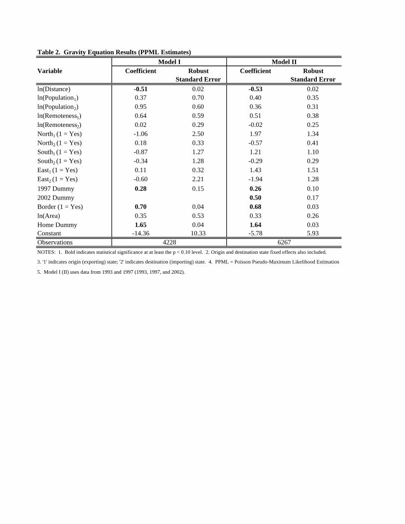
Table 2. Gravity Equation Results (PPML Estimates)
Variable Coefficient Robust Coefficient RobustStandard Error Standard Error
ln(Distance) -0.51 0.02 -0.53 0.02ln(Population1) 0.37 0.70 0.40 0.35ln(Population2) 0.95 0.60 0.36 0.31ln(Remoteness1) 0.64 0.59 0.51 0.38ln(Remoteness2) 0.02 0.29 -0.02 0.25North1 (1 = Yes) -1.06 2.50 1.97 1.34North2 (1 = Yes) 0.18 0.33 -0.57 0.41South1 (1 = Yes) -0.87 1.27 1.21 1.10South2 (1 = Yes) -0.34 1.28 -0.29 0.29East1 (1 = Yes) 0.11 0.32 1.43 1.51East2 (1 = Yes) -0.60 2.21 -1.94 1.281997 Dummy 0.28 0.15 0.26 0.102002 Dummy 0.50 0.17Border (1 = Yes) 0.70 0.04 0.68 0.03ln(Area) 0.35 0.53 0.33 0.26Home Dummy 1.65 0.04 1.64 0.03Constant -14.36 10.33 -5.78 5.93ObservationsNOTES: 1. Bold indicates statistical significance at at least the p < 0.10 level. 2. Origin and destination state fixed effects also included.
3. '1' indicates origin (exporting) state; '2' indicates destination (importing) state. 4. PPML = Poisson Pseudo-Maximum Likelihood Estimation
5. Model I (II) uses data from 1993 and 1997 (1993, 1997, and 2002).
Model I Model II
4228 6267
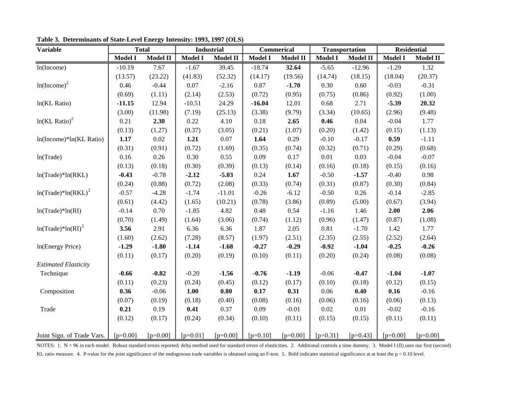
Table 3. Determinants of State-Level Energy Intensity: 1993, 1997 (OLS)Variable
Model I Model II Model I Model II Model I Model II Model I Model II Model I Model IIln(Income) -10.19 7.67 -1.67 39.45 -18.74 32.64 -5.65 -12.96 -1.29 1.32
(13.57) (23.22) (41.83) (52.32) (14.17) (19.56) (14.74) (18.15) (18.04) (20.37)ln(Income)2 0.46 -0.44 0.07 -2.16 0.87 -1.70 0.30 0.60 -0.03 -0.31
(0.69) (1.11) (2.14) (2.53) (0.72) (0.95) (0.75) (0.86) (0.92) (1.00)ln(KL Ratio) -11.15 12.94 -10.51 24.29 -16.04 12.01 0.68 2.71 -5.39 20.32
(3.00) (11.98) (7.19) (25.13) (3.38) (9.79) (3.34) (10.65) (2.96) (9.48)ln(KL Ratio)2 0.21 2.30 0.22 4.10 0.18 2.65 0.46 0.04 -0.04 1.77
(0.13) (1.27) (0.37) (3.05) (0.21) (1.07) (0.20) (1.42) (0.15) (1.13)ln(Income)*ln(KL Ratio) 1.17 0.02 1.21 0.07 1.64 0.29 -0.10 -0.17 0.59 -1.11
(0.31) (0.91) (0.72) (1.69) (0.35) (0.74) (0.32) (0.71) (0.29) (0.68)ln(Trade) 0.16 0.26 0.30 0.55 0.09 0.17 0.01 0.03 -0.04 -0.07
(0.13) (0.18) (0.30) (0.39) (0.13) (0.14) (0.16) (0.18) (0.15) (0.16)ln(Trade)*ln(RKL) -0.43 -0.78 -2.12 -5.03 0.24 1.67 -0.50 -1.57 -0.40 0.98
(0.24) (0.88) (0.72) (2.08) (0.33) (0.74) (0.31) (0.87) (0.30) (0.84)ln(Trade)*ln(RKL)2 -0.57 -4.28 -1.74 -11.01 -0.26 -6.12 -0.50 0.26 -0.14 -2.85
(0.61) (4.42) (1.65) (10.21) (0.78) (3.86) (0.89) (5.00) (0.67) (3.94)ln(Trade)*ln(RI) -0.14 0.70 -1.85 4.82 0.48 0.54 -1.16 1.46 2.00 2.06
(0.70) (1.49) (1.64) (3.06) (0.74) (1.12) (0.96) (1.47) (0.87) (1.08)ln(Trade)*ln(RI)2 3.56 2.91 6.36 6.36 1.87 2.05 0.81 -1.70 1.42 1.77
(1.60) (2.62) (7.28) (8.57) (1.97) (2.51) (2.35) (2.55) (2.52) (2.64)ln(Energy Price) -1.29 -1.80 -1.14 -1.68 -0.27 -0.29 -0.92 -1.04 -0.25 -0.26
(0.11) (0.17) (0.20) (0.19) (0.10) (0.11) (0.20) (0.24) (0.08) (0.08)Estimated Elasticity Technique -0.66 -0.82 -0.20 -1.56 -0.76 -1.19 -0.06 -0.47 -1.04 -1.07
(0.11) (0.23) (0.24) (0.45) (0.12) (0.17) (0.10) (0.18) (0.12) (0.15) Composition 0.36 -0.06 1.00 0.80 0.17 0.31 0.06 0.40 0.16 -0.16
(0.07) (0.19) (0.18) (0.40) (0.08) (0.16) (0.06) (0.16) (0.06) (0.13) Trade 0.21 0.19 0.41 0.37 0.09 -0.01 0.02 0.01 -0.02 -0.16
(0.12) (0.17) (0.24) (0.34) (0.10) (0.11) (0.15) (0.15) (0.11) (0.11)
Joint Sign. of Trade Vars. [p=0.00] [p=0.00] [p=0.01] [p=0.00] [p=0.10] [p=0.00] [p=0.31] [p=0.43] [p=0.00] [p=0.00]NOTES: 1. N = 96 in each model. Robust standard errors reported; delta method used for standard errors of elasticities. 2. Additional controls a time dummy. 3. Model I (II) uses our first (second) KL ratio measure. 4. P-value for the joint significance of the endogenous trade variables is obtained using an F-test. 5. Bold indicates statistical significance at at least the p < 0.10 level.
ResidentialTotal Industrial Commerical Transportation
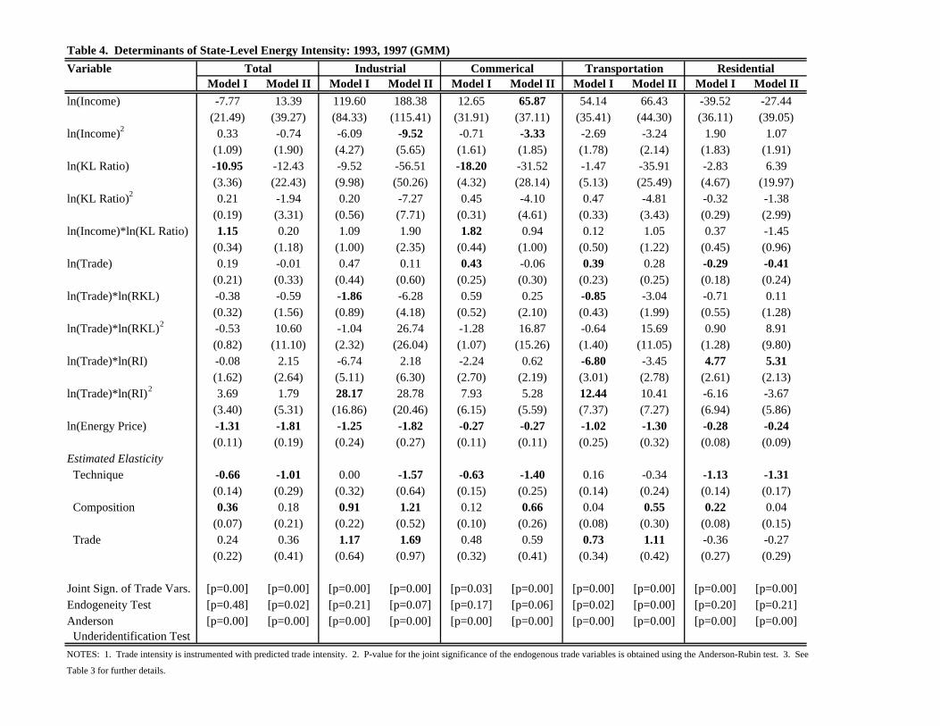
Table 4. Determinants of State-Level Energy Intensity: 1993, 1997 (GMM)Variable
Model I Model II Model I Model II Model I Model II Model I Model II Model I Model IIln(Income) -7.77 13.39 119.60 188.38 12.65 65.87 54.14 66.43 -39.52 -27.44
(21.49) (39.27) (84.33) (115.41) (31.91) (37.11) (35.41) (44.30) (36.11) (39.05)ln(Income)2 0.33 -0.74 -6.09 -9.52 -0.71 -3.33 -2.69 -3.24 1.90 1.07
(1.09) (1.90) (4.27) (5.65) (1.61) (1.85) (1.78) (2.14) (1.83) (1.91)ln(KL Ratio) -10.95 -12.43 -9.52 -56.51 -18.20 -31.52 -1.47 -35.91 -2.83 6.39
(3.36) (22.43) (9.98) (50.26) (4.32) (28.14) (5.13) (25.49) (4.67) (19.97)ln(KL Ratio)2 0.21 -1.94 0.20 -7.27 0.45 -4.10 0.47 -4.81 -0.32 -1.38
(0.19) (3.31) (0.56) (7.71) (0.31) (4.61) (0.33) (3.43) (0.29) (2.99)ln(Income)*ln(KL Ratio) 1.15 0.20 1.09 1.90 1.82 0.94 0.12 1.05 0.37 -1.45
(0.34) (1.18) (1.00) (2.35) (0.44) (1.00) (0.50) (1.22) (0.45) (0.96)ln(Trade) 0.19 -0.01 0.47 0.11 0.43 -0.06 0.39 0.28 -0.29 -0.41
(0.21) (0.33) (0.44) (0.60) (0.25) (0.30) (0.23) (0.25) (0.18) (0.24)ln(Trade)*ln(RKL) -0.38 -0.59 -1.86 -6.28 0.59 0.25 -0.85 -3.04 -0.71 0.11
(0.32) (1.56) (0.89) (4.18) (0.52) (2.10) (0.43) (1.99) (0.55) (1.28)ln(Trade)*ln(RKL)2 -0.53 10.60 -1.04 26.74 -1.28 16.87 -0.64 15.69 0.90 8.91
(0.82) (11.10) (2.32) (26.04) (1.07) (15.26) (1.40) (11.05) (1.28) (9.80)ln(Trade)*ln(RI) -0.08 2.15 -6.74 2.18 -2.24 0.62 -6.80 -3.45 4.77 5.31
(1.62) (2.64) (5.11) (6.30) (2.70) (2.19) (3.01) (2.78) (2.61) (2.13)ln(Trade)*ln(RI)2 3.69 1.79 28.17 28.78 7.93 5.28 12.44 10.41 -6.16 -3.67
(3.40) (5.31) (16.86) (20.46) (6.15) (5.59) (7.37) (7.27) (6.94) (5.86)ln(Energy Price) -1.31 -1.81 -1.25 -1.82 -0.27 -0.27 -1.02 -1.30 -0.28 -0.24
(0.11) (0.19) (0.24) (0.27) (0.11) (0.11) (0.25) (0.32) (0.08) (0.09)Estimated Elasticity Technique -0.66 -1.01 0.00 -1.57 -0.63 -1.40 0.16 -0.34 -1.13 -1.31
(0.14) (0.29) (0.32) (0.64) (0.15) (0.25) (0.14) (0.24) (0.14) (0.17) Composition 0.36 0.18 0.91 1.21 0.12 0.66 0.04 0.55 0.22 0.04
(0.07) (0.21) (0.22) (0.52) (0.10) (0.26) (0.08) (0.30) (0.08) (0.15) Trade 0.24 0.36 1.17 1.69 0.48 0.59 0.73 1.11 -0.36 -0.27
(0.22) (0.41) (0.64) (0.97) (0.32) (0.41) (0.34) (0.42) (0.27) (0.29)
Joint Sign. of Trade Vars. [p=0.00] [p=0.00] [p=0.00] [p=0.00] [p=0.03] [p=0.00] [p=0.00] [p=0.00] [p=0.00] [p=0.00]Endogeneity Test [p=0.48] [p=0.02] [p=0.21] [p=0.07] [p=0.17] [p=0.06] [p=0.02] [p=0.00] [p=0.20] [p=0.21]Anderson [p=0.00] [p=0.00] [p=0.00] [p=0.00] [p=0.00] [p=0.00] [p=0.00] [p=0.00] [p=0.00] [p=0.00] Underidentification TestNOTES: 1. Trade intensity is instrumented with predicted trade intensity. 2. P-value for the joint significance of the endogenous trade variables is obtained using the Anderson-Rubin test. 3. See
Table 3 for further details.
ResidentialTotal Industrial Commerical Transportation
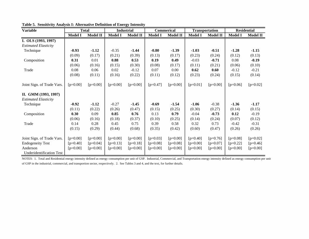
Table 5. Sensitivity Analysis I: Alternative Definition of Energy Intensity Variable
Model I Model II Model I Model II Model I Model II Model I Model II Model I Model III. OLS (1993, 1997)Estimated Elasticity Technique -0.93 -1.12 -0.35 -1.44 -0.80 -1.39 -1.03 -0.51 -1.28 -1.15
(0.09) (0.17) (0.21) (0.39) (0.13) (0.17) (0.23) (0.24) (0.12) (0.13) Composition 0.31 0.01 0.88 0.53 0.19 0.49 -0.03 -0.71 0.08 -0.19
(0.06) (0.16) (0.15) (0.30) (0.08) (0.17) (0.11) (0.21) (0.06) (0.10) Trade 0.08 0.06 0.02 -0.12 0.07 0.00 0.62 0.60 -0.12 -0.21
(0.08) (0.11) (0.16) (0.22) (0.11) (0.12) (0.23) (0.24) (0.15) (0.14)
Joint Sign. of Trade Vars. [p=0.00] [p=0.00] [p=0.00] [p=0.00] [p=0.47] [p=0.00] [p=0.01] [p=0.00] [p=0.06] [p=0.02]
II. GMM (1993, 1997)Estimated Elasticity Technique -0.92 -1.12 -0.27 -1.45 -0.69 -1.54 -1.06 -0.38 -1.36 -1.17
(0.11) (0.22) (0.26) (0.47) (0.15) (0.25) (0.30) (0.27) (0.14) (0.15) Composition 0.30 0.09 0.85 0.76 0.13 0.79 -0.04 -0.73 0.12 -0.19
(0.06) (0.16) (0.18) (0.37) (0.10) (0.25) (0.14) (0.24) (0.07) (0.12) Trade 0.14 0.28 0.45 0.75 0.39 0.58 0.32 0.73 -0.42 -0.31
(0.15) (0.29) (0.44) (0.68) (0.35) (0.42) (0.60) (0.47) (0.26) (0.26)
Joint Sign. of Trade Vars. [p=0.00] [p=0.00] [p=0.00] [p=0.00] [p=0.03] [p=0.00] [p=0.40] [p=0.76] [p=0.08] [p=0.02]Endogeneity Test [p=0.40] [p=0.04] [p=0.13] [p=0.18] [p=0.08] [p=0.08] [p=0.00] [p=0.07] [p=0.22] [p=0.46]Anderson [p=0.00] [p=0.00] [p=0.00] [p=0.00] [p=0.00] [p=0.00] [p=0.00] [p=0.00] [p=0.00] [p=0.00] Underidentification TestNOTES: 1. Total and Residential energy intensity defined as energy consumption per unit of GSP. Industrial, Commercial, and Transportation energy intensity defined as energy consumption per unit of GSP in the industrial, commercial, and transportion sector, respectively. 2. See Tables 3 and 4, and the text, for further details.
ResidentialTotal Industrial Commerical Transportation
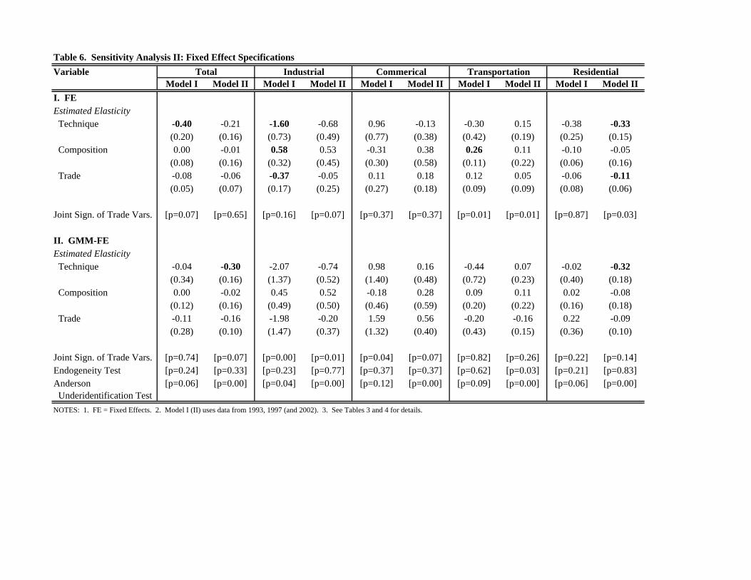
Table 6. Sensitivity Analysis II: Fixed Effect Specifications Variable
Model I Model II Model I Model II Model I Model II Model I Model II Model I Model III. FEEstimated Elasticity Technique -0.40 -0.21 -1.60 -0.68 0.96 -0.13 -0.30 0.15 -0.38 -0.33
(0.20) (0.16) (0.73) (0.49) (0.77) (0.38) (0.42) (0.19) (0.25) (0.15) Composition 0.00 -0.01 0.58 0.53 -0.31 0.38 0.26 0.11 -0.10 -0.05
(0.08) (0.16) (0.32) (0.45) (0.30) (0.58) (0.11) (0.22) (0.06) (0.16) Trade -0.08 -0.06 -0.37 -0.05 0.11 0.18 0.12 0.05 -0.06 -0.11
(0.05) (0.07) (0.17) (0.25) (0.27) (0.18) (0.09) (0.09) (0.08) (0.06)
Joint Sign. of Trade Vars. [p=0.07] [p=0.65] [p=0.16] [p=0.07] [p=0.37] [p=0.37] [p=0.01] [p=0.01] [p=0.87] [p=0.03]
II. GMM-FEEstimated Elasticity Technique -0.04 -0.30 -2.07 -0.74 0.98 0.16 -0.44 0.07 -0.02 -0.32
(0.34) (0.16) (1.37) (0.52) (1.40) (0.48) (0.72) (0.23) (0.40) (0.18) Composition 0.00 -0.02 0.45 0.52 -0.18 0.28 0.09 0.11 0.02 -0.08
(0.12) (0.16) (0.49) (0.50) (0.46) (0.59) (0.20) (0.22) (0.16) (0.18) Trade -0.11 -0.16 -1.98 -0.20 1.59 0.56 -0.20 -0.16 0.22 -0.09
(0.28) (0.10) (1.47) (0.37) (1.32) (0.40) (0.43) (0.15) (0.36) (0.10)
Joint Sign. of Trade Vars. [p=0.74] [p=0.07] [p=0.00] [p=0.01] [p=0.04] [p=0.07] [p=0.82] [p=0.26] [p=0.22] [p=0.14]Endogeneity Test [p=0.24] [p=0.33] [p=0.23] [p=0.77] [p=0.37] [p=0.37] [p=0.62] [p=0.03] [p=0.21] [p=0.83]Anderson [p=0.06] [p=0.00] [p=0.04] [p=0.00] [p=0.12] [p=0.00] [p=0.09] [p=0.00] [p=0.06] [p=0.00] Underidentification TestNOTES: 1. FE = Fixed Effects. 2. Model I (II) uses data from 1993, 1997 (and 2002). 3. See Tables 3 and 4 for details.
ResidentialTotal Industrial Commerical Transportation
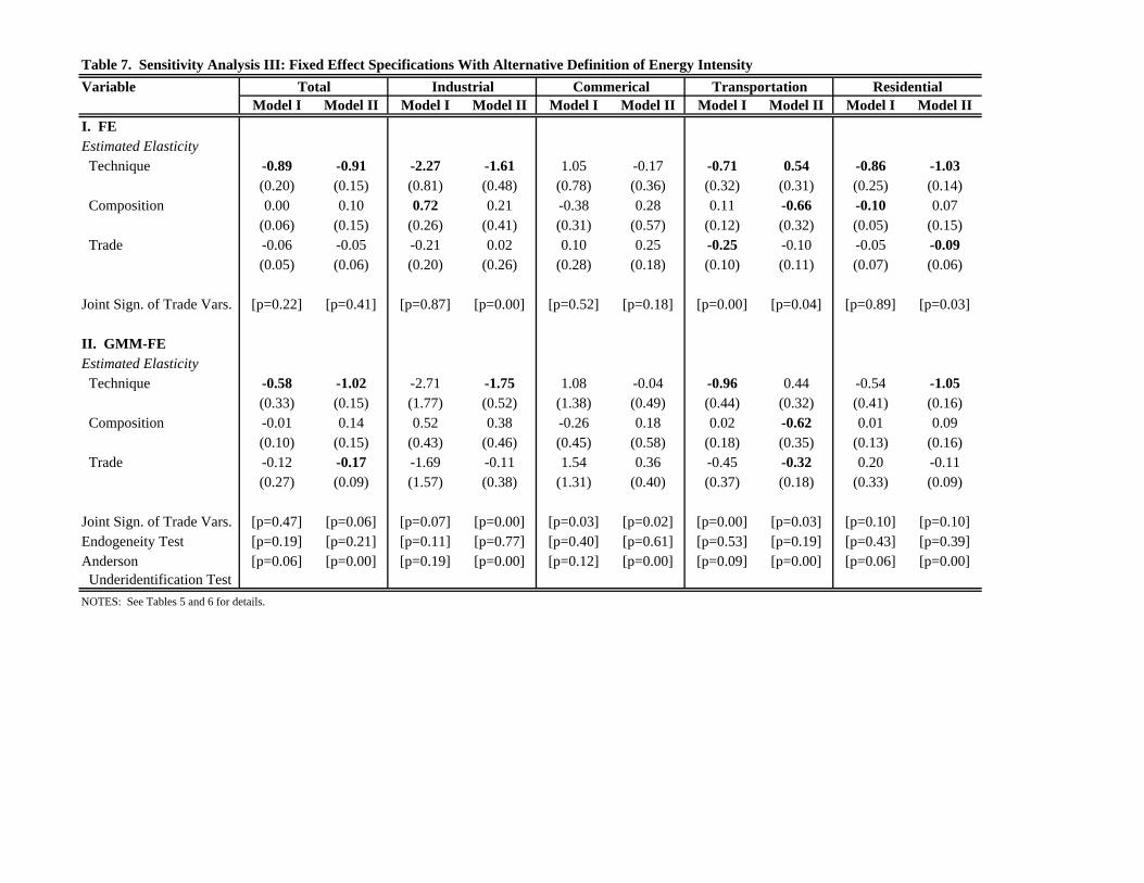
Table 7. Sensitivity Analysis III: Fixed Effect Specifications With Alternative Definition of Energy Intensity Variable
Model I Model II Model I Model II Model I Model II Model I Model II Model I Model III. FEEstimated Elasticity Technique -0.89 -0.91 -2.27 -1.61 1.05 -0.17 -0.71 0.54 -0.86 -1.03
(0.20) (0.15) (0.81) (0.48) (0.78) (0.36) (0.32) (0.31) (0.25) (0.14) Composition 0.00 0.10 0.72 0.21 -0.38 0.28 0.11 -0.66 -0.10 0.07
(0.06) (0.15) (0.26) (0.41) (0.31) (0.57) (0.12) (0.32) (0.05) (0.15) Trade -0.06 -0.05 -0.21 0.02 0.10 0.25 -0.25 -0.10 -0.05 -0.09
(0.05) (0.06) (0.20) (0.26) (0.28) (0.18) (0.10) (0.11) (0.07) (0.06)
Joint Sign. of Trade Vars. [p=0.22] [p=0.41] [p=0.87] [p=0.00] [p=0.52] [p=0.18] [p=0.00] [p=0.04] [p=0.89] [p=0.03]
II. GMM-FEEstimated Elasticity Technique -0.58 -1.02 -2.71 -1.75 1.08 -0.04 -0.96 0.44 -0.54 -1.05
(0.33) (0.15) (1.77) (0.52) (1.38) (0.49) (0.44) (0.32) (0.41) (0.16) Composition -0.01 0.14 0.52 0.38 -0.26 0.18 0.02 -0.62 0.01 0.09
(0.10) (0.15) (0.43) (0.46) (0.45) (0.58) (0.18) (0.35) (0.13) (0.16) Trade -0.12 -0.17 -1.69 -0.11 1.54 0.36 -0.45 -0.32 0.20 -0.11
(0.27) (0.09) (1.57) (0.38) (1.31) (0.40) (0.37) (0.18) (0.33) (0.09)
Joint Sign. of Trade Vars. [p=0.47] [p=0.06] [p=0.07] [p=0.00] [p=0.03] [p=0.02] [p=0.00] [p=0.03] [p=0.10] [p=0.10]Endogeneity Test [p=0.19] [p=0.21] [p=0.11] [p=0.77] [p=0.40] [p=0.61] [p=0.53] [p=0.19] [p=0.43] [p=0.39]Anderson [p=0.06] [p=0.00] [p=0.19] [p=0.00] [p=0.12] [p=0.00] [p=0.09] [p=0.00] [p=0.06] [p=0.00] Underidentification TestNOTES: See Tables 5 and 6 for details.
ResidentialTotal Industrial Commerical Transportation
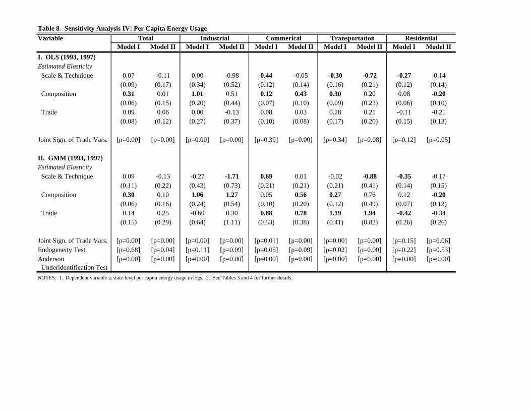
Table 8. Sensitivity Analysis IV: Per Capita Energy Usage Variable
Model I Model II Model I Model II Model I Model II Model I Model II Model I Model III. OLS (1993, 1997)Estimated Elasticity Scale & Technique 0.07 -0.11 0.00 -0.98 0.44 -0.05 -0.30 -0.72 -0.27 -0.14
(0.09) (0.17) (0.34) (0.52) (0.12) (0.14) (0.16) (0.21) (0.12) (0.14) Composition 0.31 0.01 1.01 0.51 0.12 0.43 0.30 0.20 0.08 -0.20
(0.06) (0.15) (0.20) (0.44) (0.07) (0.10) (0.09) (0.23) (0.06) (0.10) Trade 0.09 0.06 0.00 -0.13 0.08 0.03 0.28 0.21 -0.11 -0.21
(0.08) (0.12) (0.27) (0.37) (0.10) (0.08) (0.17) (0.20) (0.15) (0.13)
Joint Sign. of Trade Vars. [p=0.00] [p=0.00] [p=0.00] [p=0.00] [p=0.39] [p=0.00] [p=0.34] [p=0.08] [p=0.12] [p=0.05]
II. GMM (1993, 1997)Estimated Elasticity Scale & Technique 0.09 -0.13 -0.27 -1.71 0.69 0.01 -0.02 -0.88 -0.35 -0.17
(0.11) (0.22) (0.43) (0.73) (0.21) (0.21) (0.21) (0.41) (0.14) (0.15) Composition 0.30 0.10 1.06 1.27 0.05 0.56 0.27 0.76 0.12 -0.20
(0.06) (0.16) (0.24) (0.54) (0.10) (0.20) (0.12) (0.49) (0.07) (0.12) Trade 0.14 0.25 -0.60 0.30 0.88 0.78 1.19 1.94 -0.42 -0.34
(0.15) (0.29) (0.64) (1.11) (0.53) (0.38) (0.41) (0.82) (0.26) (0.26)
Joint Sign. of Trade Vars. [p=0.00] [p=0.00] [p=0.00] [p=0.00] [p=0.01] [p=0.00] [p=0.00] [p=0.00] [p=0.15] [p=0.06]Endogeneity Test [p=0.68] [p=0.04] [p=0.11] [p=0.09] [p=0.05] [p=0.09] [p=0.02] [p=0.00] [p=0.22] [p=0.53]Anderson [p=0.00] [p=0.00] [p=0.00] [p=0.00] [p=0.00] [p=0.00] [p=0.00] [p=0.00] [p=0.00] [p=0.00] Underidentification TestNOTES: 1. Dependent variable is state-level per capita energy usage in logs. 2. See Tables 3 and 4 for further details.
ResidentialTotal Industrial Commerical Transportation
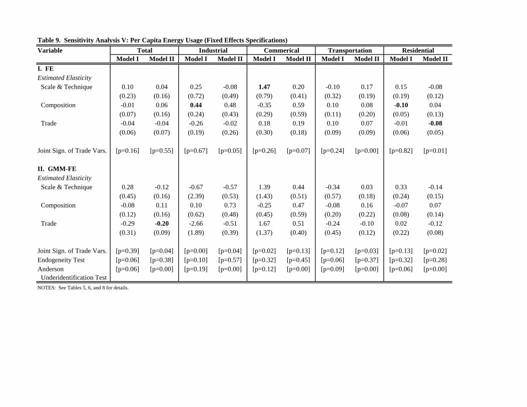
Table 9. Sensitivity Analysis V: Per Capita Energy Usage (Fixed Effects Specifications)Variable
Model I Model II Model I Model II Model I Model II Model I Model II Model I Model III. FEEstimated Elasticity Scale & Technique 0.10 0.04 0.25 -0.08 1.47 0.20 -0.10 0.17 0.15 -0.08
(0.23) (0.16) (0.72) (0.49) (0.79) (0.41) (0.32) (0.19) (0.19) (0.12) Composition -0.01 0.06 0.44 0.48 -0.35 0.59 0.10 0.08 -0.10 0.04
(0.07) (0.16) (0.24) (0.43) (0.29) (0.59) (0.11) (0.20) (0.05) (0.13) Trade -0.04 -0.04 -0.26 -0.02 0.18 0.19 0.10 0.07 -0.01 -0.08
(0.06) (0.07) (0.19) (0.26) (0.30) (0.18) (0.09) (0.09) (0.06) (0.05)
Joint Sign. of Trade Vars. [p=0.16] [p=0.55] [p=0.67] [p=0.05] [p=0.26] [p=0.07] [p=0.24] [p=0.00] [p=0.82] [p=0.01]
II. GMM-FEEstimated Elasticity Scale & Technique 0.28 -0.12 -0.67 -0.57 1.39 0.44 -0.34 0.03 0.33 -0.14
(0.45) (0.16) (2.39) (0.53) (1.43) (0.51) (0.57) (0.18) (0.24) (0.15) Composition -0.08 0.11 0.10 0.73 -0.25 0.47 -0.08 0.16 -0.07 0.07
(0.12) (0.16) (0.62) (0.48) (0.45) (0.59) (0.20) (0.22) (0.08) (0.14) Trade -0.29 -0.20 -2.66 -0.51 1.67 0.51 -0.24 -0.10 0.02 -0.12
(0.31) (0.09) (1.89) (0.39) (1.37) (0.40) (0.45) (0.12) (0.22) (0.08)
Joint Sign. of Trade Vars. [p=0.39] [p=0.04] [p=0.00] [p=0.04] [p=0.02] [p=0.13] [p=0.12] [p=0.03] [p=0.13] [p=0.02]Endogeneity Test [p=0.06] [p=0.38] [p=0.10] [p=0.57] [p=0.32] [p=0.45] [p=0.06] [p=0.37] [p=0.32] [p=0.28]Anderson [p=0.06] [p=0.00] [p=0.19] [p=0.00] [p=0.12] [p=0.00] [p=0.09] [p=0.00] [p=0.06] [p=0.00] Underidentification TestNOTES: See Tables 5, 6, and 8 for details.
ResidentialTotal Industrial Commerical Transportation