Submerged Vanes for Flow Control and Bank Protection...

SUBMERGED VANES FOR FLOW CONTROL AND BANK PROTECTION IN STREAMS

by

A. Jacob Odgaard and Hong-Yuan E. Lee

submitted to

the Highway Division of the Iowa Department of Transportation and

the Iowa Highway Research Board Project HR-255

IIHR Report No. 279

Iowa Institute of Hydraulic Research The University of Iowa Iowa City, Iowa 52242

July 1984

ACKNOWLEDGEMENTS

This investigation was sponsored by the Iowa Highway Research

Board of the Iowa Department of Transportation. The authors are

grateful for !DOT' s support and they wish to express their special

thanks to Messrs. Vernon Marks and Mark Looschen, !DOT, for

providing help at various stages of this project. The authors also

wish to acknowledge the support provided by I !HR' s mechanical and

electronic shops, in particular by Messrs. James R. Goss and Michael

Kundert, who assisted on the fie 1 d surveys; Mr. James Cramer who

constructed specialized electronic data acquisition equipment for

the model tests; and Mr. Dale c. Harris who supervised the laborious

mixing of the sediment grades used in the model tests. The data on

fl ow and bed characteristics obtained in the model tests served as

basis for the second author's Ph.D. thesis.

Dr. John F. Kennedy's crit i ca 1 review of the manuscript was

greatly appreciated.

The opinions, findings, and conclusions of this report are

those of the authors and not necessarily those of the Highway

Division of the Iowa Department of Transportation.

ii

ABSTRACT

The study has evaluated the effectiveness of Iowa Vanes in

reducing depth and velocity near the outer bank in a curved, alluvial

channe 1 fl ow. A procedure for the design of a vane system for a

given river curve has been developed and tested in a 1 aboratory

model. The procedure has been used for the design of an Iowa-Vane

bank-protect ion structure for a section of East Ni shnabotna River

along U.S. Highway 34 at Red Oak, Iowa.

iii

TABLE Of CONTENTS

LIST OF SYMBOLS ................................................................. v

LIST OF TABLES .......... oooo•••••<><>•••••<>•••••••o•e•••••••••e•••<>••vii

LIST OF FIGURES., ............................................... o••••······ .. viii

I.. INTRODUCTION .................................................................. 1

I I.. THEORETICAL ANAL VS IS .. ...................................................... ,. • • 8

I II.

IV.

A. Vane Function ........ ., ........... """"""""""""""""""""•••ic.••••10 B. Effective Bend Radius .................................... 13 C. Lift Coefficient •••.••••.•.•••.•••..••••••••••••••.••••• 15

LABORATORY-MODEL EXPERIMENTS •••••••••••••••••••••••••••••••• 18 A.

B. c. D.

Verification of Design Relations .......................... 18 1. Uniform Bed Material ................................. 18 2. Nonuniform Bed Material .............................. 36 Vanes in Armored Channel ••••.••••••••••••••••••••••••••• 39 Rock Vanes •••••••••.•••••..••••••••.•••••••••••••••••••• 43 Discussion of Results •••.••••••••••.•.•••••••••••••••••• 45

VANE DESIGN FOR EAST NISHNABOTNA RIVER BEND ••••••••••••••••• 52 A. B.

Field Surveys .............................................. 52 Design Computations ...................................... 63

V. SUMMARY, CONCLUSIONS ANO RECOMMENOATIONS •••••••••••••••••••• 72

REFERENCES ............................................. ., ........ ., .................... 76

APPENDIX I:

APPENDIX II: Grain-Size Distributions from Field Surveys ••••••••• 79

iv

LIST OF SYMBOLS

b width of channel

CL lift-force coefficient

D particle diameter

d fl OW depth

F vane function, Eq. 10

Fo particle Froude number, Eq. 4

f Darcy-Weisbach friction factor

g acceleration due to gravity

H vane height

L vane length

N number of vanes

n exponent in the power-law velocity profile

r radius

re effective radius, Eq. 12

S longitudinal slope of water surface

Sy transverse bed slope

T torque

torque due to centrifugal acceleration

torque induced by vane

u local velocity

shear velocity (= ITJP) 0

depth-averaged velocity -u

V volume

v

a vane-angle of attack

a effective angle of attack e a' vane angle with mean-flow direction

€ downwash angle

Q deviation angle, Eq. 23

I( von Karman's constant

e Shields' parameter

p fluid density

PS density of bed material (sand)

t shear stress

t bed-shear stress 0

T radial component of < r 0

4> bend angle

Subscripts

a cross-sectional average

c centerline

vi

LIST OF TABLES

Table

1. Minimum Values of the Vane Function, F •••••••••••••••••• 13

2. Summary of Model Test Conditions at Maximum Rates . of Flow •..•••...••...•.•.••...••.••...••.•••..••••••...• 21

3, Effective-Radius Calculations for Model Tests ••••••••••• 26

4. Vane-Design Calculations for Model Tests •••••••••••••••• 27

5, Summary of Experimental Results of Vane Tests ••••••••••• 33

6. High-Flow Data from East Nishnabotna River Bend ••••••••• 57

7. Low-Flow Data from East Nishnabotna River Bend •••••••••• 58

8. Vane-Design Computations for East Nishnabotna River Bend ...................................................... 65

9. Proposed Emplacement of Vane System for East Nishnabotna River Bend ••••••••••••••••••••••••••••••.••• 71

vii

LIST OF FIGURES

Figure

1. Aerial Photo of East Nishnabotna River and U.S. Highway 34 at Red Oak, Montgomery County, Iowa, March 13, 1972 ••................•..••...••..••.....•.•... 2

2. Aerial Photo of East Nishnabotna River and U.S. Highway 34 at Red Oak, Montgomery County, Iowa, March 7, 1977 .•.••••••••••••••••••••••••••••••••••••••••••••••• 3

3. Aerial Photo of East Nishnabotna River and U.S. Highway 34 at Red Oak, Montgomery County, Iowa, August 11, 1982 •••••••••••••••••••••••••••••••••••••••••••••••• 4

4. Sequential Centerlines of East Nishnabotna River at Red Oak, Montgomery County, Iowa ••••••••••••••••••••••••••••••• 6

5. Vane Function F as a Function of Vane Height-Water Depth Ratio, H/d, for Four Values of n •••••••••••••••••••••••• 12

6. Lift Coefficients for Flat-Plate Vane ••••••••••••••••••••••••• 17

7. IIHR's Curved Sediment Flume; (a) Viewed Upstream Toward the Flume Inlet; and (b) Viewed Upstream Around the Curve ........................................................ 19

8. Layout of IIHR's Curved, Recirculating Sediment Flume, with Section Numbers and Bend Angles •••••••••••••••••••••••••• 20

9. Grain-Size Distribution for Uniform Bed Sediment, Test Series 1 and 2 ••••••••••••••••••••••••••••••••••••••••••• 22

10, Streamwise Variation of Transverse Bed Slope Development, Test Series No. 1 ••••••••••••••••••••••••••••••.• 24

11. Development of Bed Profile at Section 80, Test Series No. l •....•. 0 ............................. 0 ................ 25

12. Development of Bed Profile at Section 112, Test Series No. ! ................................ .................... 25

13. Test Series 1: Measured Radial Average-Distributions of Depth and Depth-Averaged Mean Velocity Compared with the Predicted Distributions; (a) Before Installation of Vanes; (b) After Installation of Vanes ••••••••••••••••••••• 28

14. Test Series 1 Vane Emplacement .....•... o••••••••••••••••••••••28

viii

15. Streamwise Variation of Transverse Bed Slope Develop-ment after Installation of Vanes; Test Series No. 1 ••••••••••• 30

16. Development of Bed Profiles at Section 80 after Installation of Vanes; Test Serie.s No. 1. ..................... 31

17. Development of Bed Profile at Section 112 after Installation of Vanes; Test Series No. 1 ••••••••••••••••••.••• 31


19. Test Series 2 Vane and Vane Emplacements •••••••••••••••••••••• 35

20. Grain-Size Distribution for Nonuniform Bed Sediment; Test Series No .. 3 ................................................... 37


22. Grain-size Distributions for Nonuniform Bed Sediment; Test Series No. 4 .................................................... 40

23. Test Series No. 4: Radial Average-Distributions of Depth, Depth-Averaged Mean Velocity, and Median-Grain Diameter; (a) Before Installation of Vanes; (b) After Installation of Vanes ••••••••••.••••••••••••••••••••••.••••••• 41

24. Test Series No. 4 Run 3 Vane Emplacement •••••••••••••••••••••• 41

25. Test Series No. 4: Radial Average-Distributions of Depth; (a) Before Installation of Vanes; (b) After Installation of Vanes ................................................ 44

26. Test Series No. 5: Radial Average-Distributions of Depth, and Depth-Averaged Mean Velocity between Sections 72 and 112; (a) Before Installation of Vanes; (b) After Installation of Vanes ••••••••••••••••••••••••••••••• 44

27. Test Series No. 5: Rock Vanes before Admission of Flow •••••••• 46

28. Test Series No. 5: Rock Vanes after Admission of Flow ••••••••• 46

ix

29. Naturally Formed Bed Topography in Test Series No. 4 (Looking Up st ream) .............................................. 48

30. Bed Topography in Test Series No. 4 (Looking Upstream) after Installation of 14-in. Vanes •••••••••••••••••••••••••••• 48

31. Depth Distribution at Section 112 in Test Series No. 4 Before Installation of Vanes •••••••••••••••••••••••••••••••••• 49

32. Depth Distribution at Section 112 in Test Series No. 4 After Installation of 14-in Vanes ••••••••••••••••••••••••••••• 49

33. Close-Up of Bed with 14-in. Vane (one barely visible) at Section 112 in Test Series No. 4 •••••••••••••••••••••.••••• 50

34. Bed Topography Downstream from Section 112 in Test Series No. 4 with 14-in. Vanes ................................. 50

35. Depth Distribution at Section 112 in Test Series No. 4 After Installation of 9-in. Vanes •••••••••••••••••••••••.••••• 51

36. Depth Distribution at Section 112 in Test Series No. 2 After Installation of 9-in. Vanes ••••••••••••••••••••••••••••• 51

37. Plan-View Sketch of IIHR's Sediment Flume Overlaid the East Nishnabotna River Bend at Red Oak, Using a Scale Ratio of 1:10 ••••••••••••••••••••••••••••••••••.••••••••.••••• 53

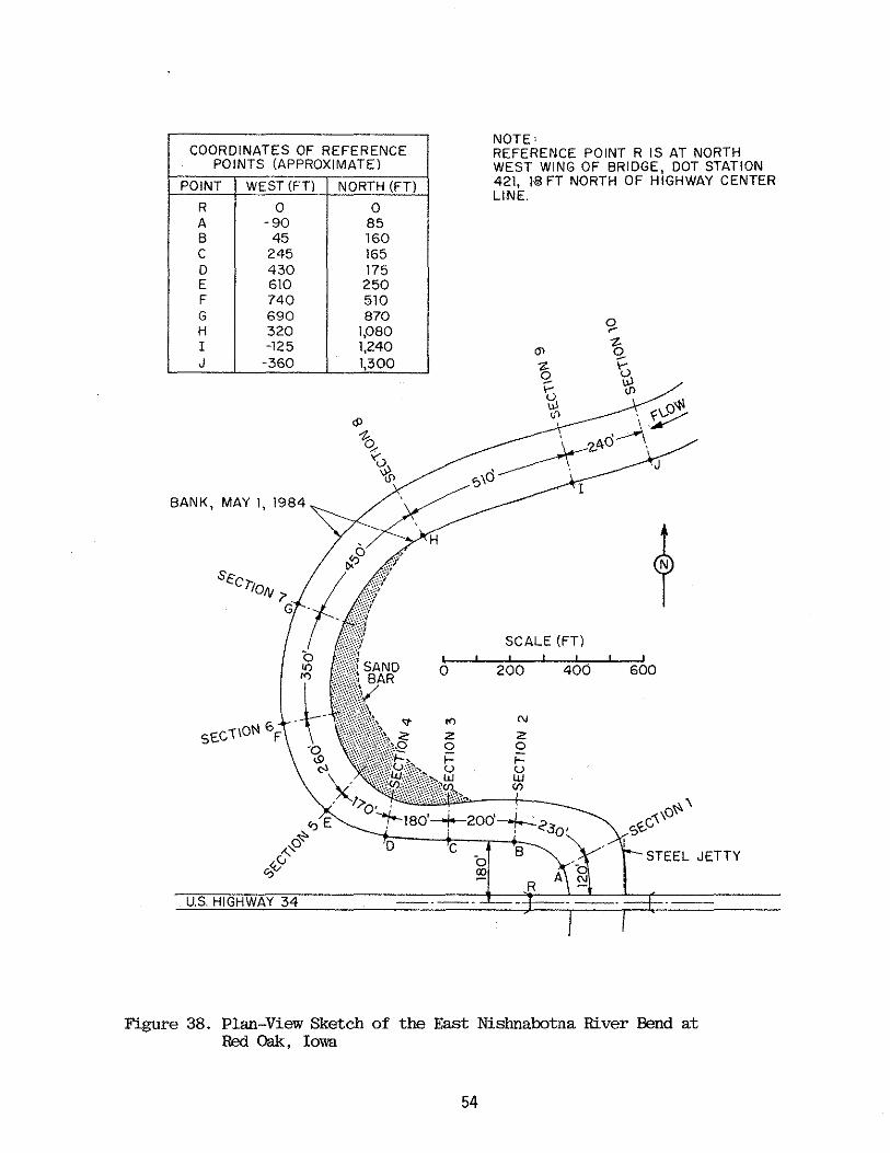
38. Plan-View Sketch of the East Nishnabotna River Bend at Red Oak, Iowa ................................................... 54

39. East Nishnabotna River on May 2, 1984, Looking Upstream from the U.S. Highway 3~ Bridge •••••••••.••••••••••••••••••••• 56

41. Sections 1 through 10 of the East Nishnabotna River Bend •• ............................................................. 59

42. Rating Curve for the U,S.G.S, Water-Stage Recorder on East Nishnabotna River at Red Oak (at Coolbaugh Street Bridge)oooo.,eeoo••••e••••••••••••oooooeooo•eooooooeoooo62

43, East Nishnabotna River on May 2, 1984, Looking Downstream toward the Highway 34 Bridge (The rock protection is along the right bank in the upper-center portion of the picture) •••••••••••••••••••••••••••••••••.••••• 64

44. Frequency Distribution for Discharge in East Nishnabotna River at Red Oak •••••••••••••••••••••••••••••••••• 68

x

45. Proposed Emplacement of Vane System for the East Nishnabotna River Bend •••••••••••••••••••••••••••••••••••••••• 70

46. Proposed Combination of Vanes and Rock Rip Rap at the Highway 34 Bridge •••..•••.•••••••••••••.••••• ., •.•••••.••.••••• 70

47. U.S. Highway 34 Bridge over East Nishnabotna River, Viewed Downstream toward Right Bank of River •••••••••••••••••• 75

48. U.S. Highway 34 Bridge over East Nishnabotna River, Viewed Downstream from Left Bank of River ••••••••••••••••••••• 75

xi

SUBMERGED VANES FOR FLOW CONTROL AND BANK PROTECTION IN STREAMS

I. INTROOUCTION

The fi na 1 report on work conducted under the St reambank Erosion

Control Evaluation and Demonstration Act of 1974 (Section 32, Public

Law 93-251) was submitted recently to Congress by the U.S. Army Corps

of Engineers (December 1981). The main conclusion of the work was

that streambank erosion continues to be a serious problem along many

of the Nation's streams and waterways, resulting in serious economic

losses of private and public lands, bridges, etc. According to this

report, approximately 148,000 bank-miles of streams and waterways are

in need of erosion protection. The cost to arrest or control this

erosion, using convention al bank protection methods currently

available, was estimated to be in the excess of $1 billion annually.

The problem is difficult because bank erosion is often the

result of a complex interaction between water and sediment in the

streams. The sediment-transport capacity and erosion potential of a

stream flow become greater with increasing boundary shear stress and

.flow velocity. Along curved reaches and in bends, the interaction

between the vertical gradient of streamwise velocity and the

curvature of the primary fl ow generates a so-called secondary or

spiralling flow, which produces larger depths and therefore also

larger velocities and boundary shear stresses near the outer

(concave) bank. The channel deepening undermines this bank, and the

larger local velocities attack it, and thus is the stage set for

river-bank erosion.

The problem in Iowa is illustrated in Figs. 1, 2, and 3, which

show aerial photos of East Ni shnabotna River at Red Oak, Montgomery

County. The photos were taken at 5-year intervals in 1972, 1977, and

1982. Over the 10-year period, a total of 20 acres of farmland was

lost by bank erosion along this 1.6-mile reach of the river. Erosion

at a comparable rate is occuring along the entire leng1!h of East

1

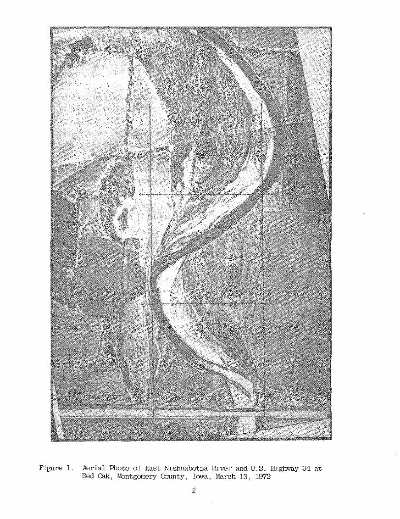
Figure 1. Aerial Photo of East Nishnabotna River and U.S. Highway 34 at Red ilik, Montgomery County, Iowa, March 13, 1972

2

Figure 2. Aerial Photo of East Nishnabotna River and U.S. Highway 34 at Red Chk, Montgomery CDunty, Iowa, March 7, 1977

3

Figure 3. Aerial Photo of East Nishnabotna River and U.S. Highway 34 at Red Oak, Montganery County, Iowa, August 11, 1982

4

Ni shnabotna River, and along a very si gni fi cant part of a 11 the

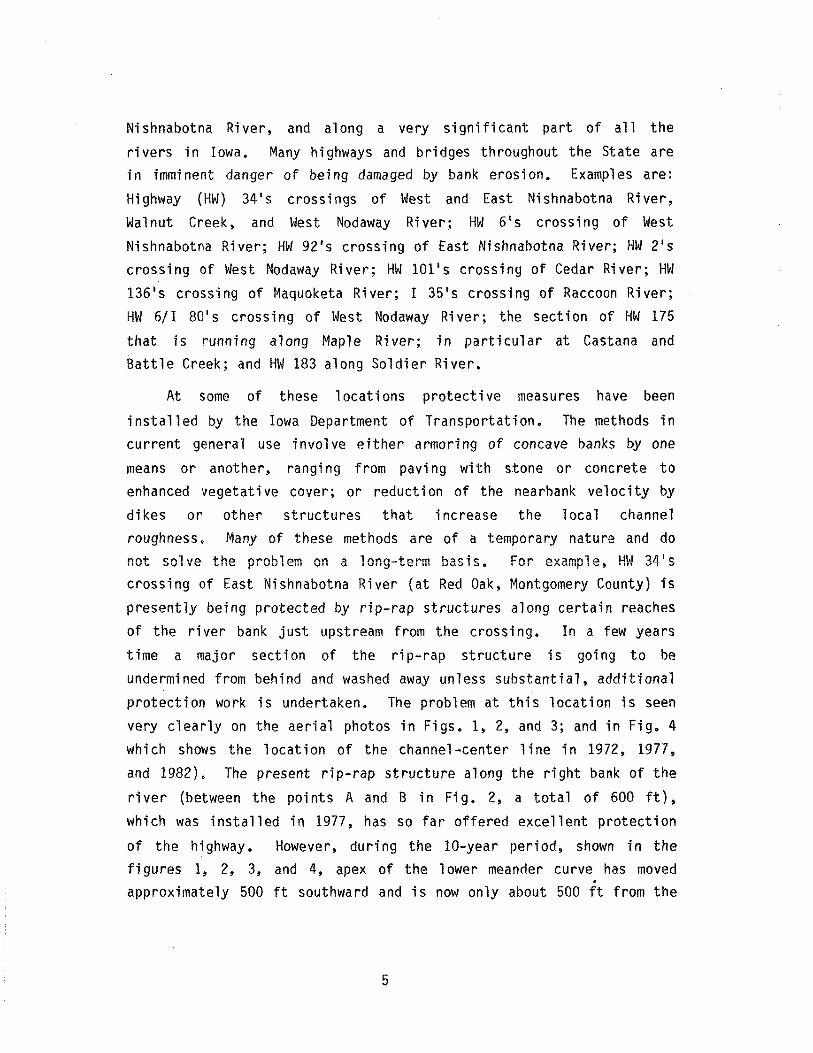
rivers in Iowa. Many highways and bridges throughout the State are

in imminent danger of being damaged by bank erosion. Examples are:

Highway (HW) 34's crossings of West and East Nishnabotna River,

Walnut Creek, and West Nodaway River; HW 6's crossing of West

Nishnabotna River; HW 92's crossing of East Nishnabotna River; HW 2's

crossing of West Nodaway River; HW lOl's crossing of Cedar River; HW

136's crossing of Maquoketa River; I 35's crossing of Raccoon River;

HW 6/1 80's crossing of West Nodaway River; the section of HW 175

that is running along Maple River; in particular at Castana and

Battle Creek; and HW 183 along Soldier River.

At some of these locations protective measures have been

i nsta 11 ed by the Iowa Department of Transportation. The methods in

current general use involve either armoring of concave banks by one

means or another, ranging from paving with stone or concrete to

enhanced vegetative cover; or reduction of the nearbank velocity by

dikes or other structures that increase the local channel

roughness. Many of these methods are of a temporary nature and do

not solve the problem on a long-term basis.. For example, HW 34 1 s

crossing of East Nishnabotna River (at Red Oak, Montgomery County) is

presently being protected by rip-rap structures along certain reaches

of the river bank just upstream from the crossing. In a few years

time a major section of the rip-rap structure is going to be

undermined from behind and washed away unless substantial, additional

protection work is undertaken. The problem at this location is seen

very clearly on the aerial photos in Figs. 1, 2, and 3; and in Fig. 4

which shows the location of the channe 1-center line in 1972, 1977,

and 1982), The present rip-rap structure along the right bank of the

river (between the points A and Bin Fig. 2, a total of 600 ft),

which was installed in 1977, has so far offered excellent protection

of the highway. However, during the 10-year period, shown in the

figures 1, 2, 3, and 4, apex of the lower meander curve has moved

approximately 500 ft southward and is now only about 500 ft from the

5

SCALE (FT)

0 200 400

..

1982 1972

·· ...

~. \ '

I

I . . 1972 . ...- 1977 / 1982

....... 7 .. ./ /./

·.

7( U.S HIGHWAY 34 f

Fig. 4 - Sequential Centerlines of East Nishnabotna River at Red Oak, Montgomery County, Iowa.

6

highway. It is obvious that the present bank protection will be

insufficient for the protection of the highway in the future. At the

present rate of bank erosion at this site, the rip-rap structure

between A and B will be undercut and 1000 ft of Highway 34, including

the highway bridge, will be seriously damaged within the next 5 to 7

years unless additional protection is provided. Problems of similar

nature are being faced at sever a 1 other highway sections and bridge

crossings in Iowa, some of which were mentioned in the preceding

paragraphs.

Many minor roads in Iowa also face this problem. Examples here

are the low-water crossings where dips in the road have been provided

to allow flood flows to pass the road. As the courses of most

streams tend to change with time, the flood flows are often seen to

attack the roads at points (away from these dips) that are not

designed to withstand the impact of high velocity flow. In such

cases there is a need for a simple inexpensive technique that can

insure that the flood flows always cross the roads at the

predesignated points.

Considering the risks that are at stake at so many sections of

Iowa's highway system, which is one of the State's major investments,

and considering the inadequacy of the protection methods that are in

current use, there appears to be an urgent need for the development

of new ideas or approaches for the safeguarding of these investments

against the erosive attack of the streams.

This study was conducted for the purpose of evaluating a new

concept for a bank-protection structure: The Iowa Vane (Odgaard and

Kennedy, 1983). The underlying idea involves countering the torque

exerted on the primary flow by its curvature and vertical velocity

gradient, thereby eliminating or significantly reducing the secondary

fl ow and thus reducing the undermining of the outer banks and the

high-velocity attack on it. The new structure consists of an array

of short, vertical, submerged vanes installed with -a certain

7

orientation on the channel bed. A relatively small number of vanes

can produce bend flows whichl are practically uniform across the

channe 1. The height of the vanes is 1 ess than ha 1f the water depth,

and their angle with the flow direction is of the order of 10°. In

this study, design relations have been established (Chapter II). The

relations, and the vanes' overall performance, have been tested in a

laboratory model under different flow and sediment conditions

(Chapter III). The results are used for the design of an Iowa-Vane

bank protection structure for a section (Fig. 3) of East Nishnabotna

River along U.S. Highway 34 at Red Oak, Iowa (Chapter IV),

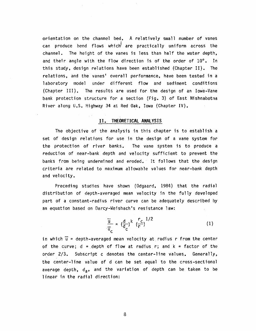
II. THEORETICAL ANALYSIS

The objective of the analysis in this chapter is to establish a

set of design relations for use in the design of a vane system for

the protection of river banks. The vane system is to produce a

reduction of near-bank depth and velocity sufficient to prevent the

banks from being undermined and eroded. It follows that the design

criteria are related to maximum allowable values for near-bank depth and velocity.

Preceding studies have shown (Odgaard, 1984) that the radial

distribution of depth-averaged mean velocity in the fully developed

part of a constant-radius river curve can be adequately described by

an equation based on Oarcy-Weisbach's resistance law:

u = (~ ) k UC C

r c 1/2 (-) r

(1)

in which u = depth-averaged mean velocity at radius r from the center

of the curve; d = depth of fl ow at radius r; and k = factor of the

order 2/3, Subscript c denotes the center-line values. Generally,

the center-1 i ne va 1 ue of d can be set equal to the cross-sect i ona 1

average depth, da, and the variation of depth can be taken to be

linear in the radial direction:

8

d = d + ST (r - r ) a c (2)

in which Sr = radial or transverse slope of the bed surface.

According to Odgaard (lg84), Sr is related to primary flow variables

by the equation

(3)

in which e = Shields' (1936) parameter; and Fo = densimetric particle Froude number defined as

ua FD=-====

p -p I _s_ gD

p

(4)

in which D =median-grain size of the bed material; g =acceleration

due to gravity; ua = cross-sectional average velocity; and p and Ps =

density of fluid and bed sediment, respectively. Substituting Eq. 2

into Eq. 1 yields the following relationship between Sr and u: " s = ~ [(u )l/k (L)l/2k _ l] (5)

T r-r - r C UC C

Hence, a criterion for u is equivalent to a criterion for Sr, and the

design objective for the vane system can be formulated as a maximum

allowable value for Sr· To reduce (or eliminate) the transverse bed

slope Sr, the vane system must reduce (or eliminate) the secondary flow in the river curve.

The effectiveness of a vane depends on the 1 ift and drag induced

by the fl ow as it passes the vane, and the height of the vane in

re 1 at ion to the water depth. (The 1 ift is the sum of the forces

(pressure and viscous) that acts normal to the free-stream direction;

the drag is the sum that acts parallel to the free-stream

direction). The lift and drag, in turn, depend on the shape of the

vane; its aspect ratio (height-length ratio); and angle of incidence

9

with the free-stream direction, a, To maximize the effectiveness of a vane design, the moment of the lift force about the centroid of the channel-cross section must be maximized and the drag force on the vane must be minimized (large drag would change the overall characteristics of the river flow increasing channel roughness, which should be avoided). In addition, the vane emplacement must be designed such that the effectiveness of the vane array as a whole is maximized. In other words, adverse interference among the vanes must be avoided (cascade effect), The following analysis provides a guide to the design of a vane system.

A. Vane Function

The secondary flow in a river curve is produced by the torque, Tc• due to the centrifugal force being distributed nonuniformly over the depth. For fully developed fl ow in a rectangular channel with

constant radius and a power-law velocity distribution, Tc is given by (Eq. 3 in Ref. 3)

T 1 -2 n+l d2b4> c = "2" P u n(n+2) {6)

in which $ = included bend angle; b = channel width; and n = velocity-profile exponent. n is related to the Darcy-Weisbach friction factor, f, by (Zimmermann and Kennedy, 1978)

(7)

in which K = von Karman's constant. (Hence, n = KU/lgsd, S = longitudinal slope of water surface). The Iowa Vanes exert a torque on the flow that is given by (Eq. 6 in Ref. 3, with 211 sina =cl)

1 -2 2 H {2+n)/n l_n_+_l}2 n+l H TV= 4 CLPU Ld (-d) [!iTi1+2T- -n-d] N (8)

in which CL = lift coefficient; L = vane length; H = vane height; and

JO

N = number of vanes. To eliminate the secondary flow that is

generating the transverse bed slope, Sr, the vanes must,. exert a

torque that balances the driving torque, Tc. Equating Tc and Tv

yields

F is a function (termed the vane function) of n and H/d given by

1 F = H 2/n H (10)

(Cf) [(n+l)-(n+2) crJ Fri. 9 yields the total vane area (lifting surface) needed per unit

surface area of channel bed [NHL/(rc~b)] as a function of the radius

d0rrt:h ratio of the channel, rc/d; lift coefficient, cl; and the vane

function, F = F(n,H/d). The vane function is graphed in Fig. 5. It

i~ 5een that for given value of H/d the value of F, and therefore the

required lifting surface, increases when n decreases (i.e., when the

frictional resistance increases). The vane function has its minimum

at H/d = 2(n+l)/(n+2)2:

-2/n F = n+2 [2(n+l)J

min n(n+l) ~ ( 11)

Corresponding values of Fmin• H/d, and n are listed in Table 1. The

vane function is seen to be relatively insensitive to variations of

H/d over a fairly large range of Hid-values. For example, for n = 4,

F is within 20% of its minimum value (the design value) when H/d is

within the range of O .12 < H/d < 0 .48 (that is, when the water depth

is between 2 and 8 times the vane height). A typical river bend

11

1.0

lL 0.8

z 0 1-(.)

z 0.6 :::> lL

w z <J: > 0.4

0.2

n =4 5 6 8

0.0 L__j___l_._j___L__L__L__L__L__L-__J

0.0 0.2 0.4 0.6 0.8 1.0 H/d

Figure 5. Vane Function F as a Function of Vane Height-Water Depth Ratio, H/d, for Four Values of n

12

Table 1 - Minimum Values of the Vane Function, F.

Velocity Minimum Value of H/d-range within profile value of H/d at which which F ~ 1.2 Fmin

exponent, F' Fm; n F = Fm; n n

4 0.57 0,28 0.12-0.48 5 0.41 0.24 0,09-0.46 6 0.32 0.22 0.07-0.45 7 0.26 0.20 0.06-0.43 8 0.21 0.18 0.05-0.40

would have an rc/d ratio of about 100 and an n value of about 4.

With H/d = 0.28 (yielding F = 0.57), and cl= 1 (the selection of the

CL - value will be discussed in Section C), Eq. 9 shows that the

total lifting surface required would then be 1.14% of the surface

area of the channel bend. With a width-depth ratio, b/d, of 10,

which is typical, the total length of vanes required (NL) is 41% of

the length of the channel to be protected (re~). Adding 20% to allow

for the aforementioned fluctuation in water depth yields the

percentages 1,37 and 49, respectively.

B. Effective Bend Radius

Eq. 9 applies to ful Ty-developed, constant-radius bend flow.

Most natural bends are not constant-radius bends, nor is the flow in

them fully deve 1 oped, and Eq. 9 cannot be used. However, if the

channel's radial distribution of depth is known (measured) an

effective-radius concept can be used for the vane design. The

effective radius, re• is the radius at which a fully-developed,

constant-radius bend fl ow would form a transverse bed slope of the

known or measured magnitude. According to Eq. 3, re is then related

to the transverse bed slope, ST, by the equation

13

(12)

The vanes must produce a torque that balances the torque, Tc, responsible for this transverse bed slope. The driving torque in

this case is given by Eq. 6 with</> = <l>e' where <l>e = effective

angle (the angle corresponding to the effective radius, re).

design relation, obtained by equating Tc and Tv, then reads

1 r (-;fl ( r NfHb) = F °Z CL

or, since re</> e = r c<l>, e e

1 r (~)(NLH ) = F 2 CL d ~ c

bend

The

(13)

(14)

Eqs. 9 and 14 are based on complete elimination of the secondary

current and the achievement of zero transverse bed slope. Practical

considerations may not justify such an ideal (asymptotic)

objective. Also, the vane height or the total number of vanes (or

both) may become a practical problem, in which case lower or fewer

vanes (or both) may have to be combined with minimal slope protection

on the banks. A vane system would be adequate if it can make the

bank-shear stress stay below the critical value at all flow rates.

If the critical bank-shear stress is relatively high due to slope

protection, some transverse slope on the river bed may be

acceptable. If the acceptable transverse bed slope is Sro• the vanes must produce a torque that can reduce the slope from Sr to Sro, or,

according to Eq. 12, increase the effective radius from re to reo• where

d ./- a

reo = 4.8 e FD -s:;:--To

(15)

The required 1 ift i ng surface ( NLH) would then be obtained as the

difference between the 1 ift i ng surface required for zeroing Sr and

that required for zeroing Sr0 :

14

2 1 1 NHL = - Fr <i>bd (r - -r-) cL c e eo

(16)

C. Lift Coefficient

If the flow around the vane were ideal and two-dimensional, the

Kutta condition (Sabersky and Acosta, 1964) would yield

c = 2n sin o: (17) L

in which o: = the vane's angle of attack with the mean flow. However,

the flow around the vane is not ideal nor two-dimensional. As the

aspect ratio, H/L, decreases, cL decreases relative to the value

given by Eq. 17. Also, with increasing value of o:, flow separation

becomes more and more important increasing the drag and decreasing

the lift. The decrease of cL with decreasing aspect ratio is due

partly to the tip vortices (the vortices trailing the upper edge of

the vane), which induce a downward motion (downwash) in the fluid

passing over the vane. The downwash has the effect of turning the

undisturbed free-stream velocity, so the effective angle of attack is

reduced by a certain angle e to

°'e = o:-e ( 18)

Nothing is known about the va 1 ue of £ for sma 11-aspect-rat io foils

that are wa 11- (or bottom-) attched. For a finite-span airfoil in

undisturbed freestream air, the downwash angle s can be calculated by

(Bertin and Smith, 1979, pp. 170-174)

(19)

This equation is obtained by using an elliptic spanwise circulation

distribution in the relationship between circulation and lift

coefficient. For a finite-span airfoil, the geometric angle of

attack is then given by

15

cl a=a+~~~ e "(H/L)

(20)

If two airfoils have the same lift coefficient and effective angle of

attack, but different aspect ratios, Hi/L1, and H2/L2, their

geometric angles of attack, a 1 and a 2, are thus related by the

equation

(21)

The validity of Eqs. 20 and 21 have been verified experimentally

(Bertin and Smith, 1979) for airfoils with aspect ratio greater than

or equal to one. For a bottom-attached flat plate it is tentatively

assumed that Eq. 17 applies at 1 arge aspect ratios, and that the

downwash angle is ha 1f that given by Eq. 19 (as a bottom-attached

foil has only one edge with tip vortices). Using Eq. 21, the lift

coefficient can then be determined as a function of a and H/L (Fig.

6). Note that although the aforementioned assumptions are

reasonable, they have not been verified experimentally.

The angle a to be used for the calculations of CL is the angle

as seen by the fluid approaching the vane. Because of the

centrifugal acceleration, the near-bed velocity distribution (the

velocity distribution seen by the vane) is skewed toward the inside

of the bend. The angle the near-bed velocity forms with the mean~

flow direction, o, is given by (Falcon, 1979)

T

o = arc tan (.....!:.) TO

(22)

in which T = bed-shear stress; and T = radial component of T •

o 22-2 r -20 Substituting T = (K /n ) pu and T = P (n+l)/[n(n+2)] (d/rel u o r (Falcon, 1979) into Eq. 22 yields

o = arc tan [.!_ n(n+l) .<!__] 2 n+2 r (23)

K e

16

2.5 ~---------~----~----~--·---

..J u

2.0

!--' z 1.5 w u LL LL w 0 u 1.0 f-LL _J

0.5

5

CL= 2vsina

H/L = 2.0

10 15 20 ANGLE OF ATTACK, a (degrees)

Figure 6. Llft Coefficients for Flat-Plate Vane

17

25

Hence, if a vane is placed at an angle with the mean-flow direction

of a', the angle a to be used for the calculation of CL is given by

a =a' +o (24)

III. LABORATORY-MODEL EXPERIMENTS

The validity of the foregoing design relations, and the

effectiveness of the vanes in producing more uniform 1atera1

distributions of depth and velocity, were tested in IIHR's 250-ft

long, 8-ft wide, and 2-ft deep, curved, recirculating sediment flume

(Fig. 7) Fig. 8 shows the layout of the flume with section numbers,

which are the distances, in feet, from the inlet, measured along the

inner flume wa 11. The center-1 i ne radius of the curved part of the

flume is 43 ft. The instrumentation and measurement technique were

described by Odgaard and Kennedy (1983). Tests were conducted with

both uniform and nonuniform bed material with smooth and rough banks;

with different vane lengths and emplacement; and with vanes composed

of modeled sheet piling and steep-sided windrows of rock. A summary

of test conditions is given in Table 2.

A. Verification of Design Relations

The formula for the transverse bed slope, Eq. 12, and the vane

design relations, Eqs. 9, 14, or 16, were tested in three series of

experiments with two different grades of bed sediment.

1. Unifonn Bed Sediment - In Test Series No. 1, the sediment

was sand with a median diameter of 0.30 mm and a geometric standard

deviation of 1.45 (Fig. 9). The sand was placed in the flume in a 9-in. thick layer throughout. After about an hour of gentle wetting,

the sand bed was subjected to a fl ow of 5 .2 cfs for a period of 160

hours. The bed topography was measured after periods of 10, 20, 40,

18

(a)

(b)

Figure 7. IIHR' s Quved Sediment Flume; (a) Viewed Upstream Toward the Flume Inlet; and (b) Viewed Upstream Around the Olrve

19

\ I I \ I

\ 0 ;;; 0

"' " !'! <e' '

., '

'- ~ .,., / '

"'o •• /' 0 ' ',, "' "' 0

"' 0 0 00

q, 0 >? !] 0 ,~'/, ,>? <t> 0

' ~o o ~ ,, .o ,.o 6. ' 0

,~o

,rooo , ss 100 110°

, .. oo 180°

48 t_ BENO ANGLE 176 ----

·40 184 r· LsECTION NUMBER

'--'--0 4 a 12 IG 20

SCALE IN FEET

:Figure 8, Layout of IIHR' s Curved, Recirculating Sediment Flume, with Section Numbers and Bend Angles

20

Table 2. summary of Model Test Conditions at Maximum Rates of Flow

Test Flow rate, Cross-sectional Median- Geometric Longitudinal Velocity- Cross-Sectional Condition Series in cubic average depth, grain standard slope of profile average velocity, of channel

feet per d8 , in feet diameter, D deviation water exponent u6 , in feet side wall second in millimeters of bed material surface per second

1 5.2 0.50 0.30 1.45 0.00104 4.0 1.30 smooth

2 6.0 0.54 0.30 1.45 0.00146 3.5 1.40 rough

3 5.8 0.47 0.90 1.90 0.00063 6.5 1.56 smooth

4,5 5.8 0.50 2.7 2.78 0.00217 3.1 1.45 rough

N ~

99.5 99 98

w N 95 (f)

0 90 w ~ 80 u ,, 0 70 z z 60 <( 50 I t- 40 0:: 30 w z LL 20 t-z 10 w u 0:: 5 w a..

2

0.5 O.l 0.2 0.5 1.0 2.0

SIZE, IN MILLIMETERS

Figure 9. Grain-Size Distribution for Unifonn Bed Sediment, Test Series 1 and 2

22

5.0

80, and 160 hours. Each time, the depth was measured at 19 points

across each of 25 sections throughout the bend. At each section the

topography was characterized by the transverse slope of the bed as

determined by linear regression. (The actual slope was not complely

constant across the channel especially not at the end of the time

period; however, the test objective did not call for any higher

degree of mathemat i ca 1 sophistication). The transverse bed slope

changed quite rapidly within the first 10 hours after the start of

the test (Fig. 10). After 10 hours, the changes were minor. The

maxi mum trans verse bed s 1 ope ( O .092) deve 1 oped at Sections 80 and

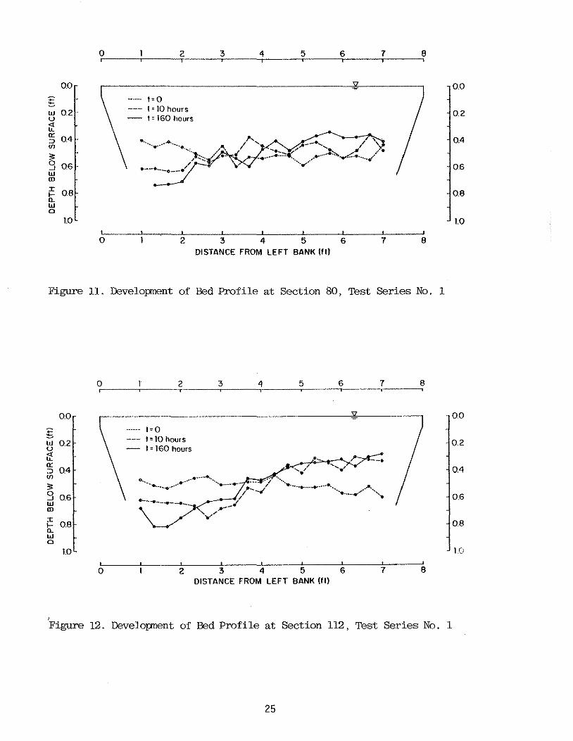
84. Fi gs. 11 and 12 show the bed profile at Sections 80 and 112 at

times 0, 10, and 160 hours. Over the 160-hour period, a total of 30

ft3 of sand was moved from the outer half of the channel to the inner

half generating point bars and scour holes, typical features of an

alluvial channel bend. The longitudinal slope of the water surface,

and the cross-sectional average depth and velocity were measured to

be 0.00104, 0,50 ft, and 1.30 ft/sec, respectively. Thus, Fa = 5.67,

n = 4.0, and u* = KUa/n = 0.10 ft/sec (u* = shear velocity = IT/p), The value of the boundary Reynolds number, u*D/v (v =

kinematic viscosity), was approximately 12 yielding (from Shields'

curve) a Shields parameter of G = 0,04. Based on these flow data,

Eq. 12 predicts a transverse bed slope of ST = 0.063. This slope is

seen (Fi gs. 10 and 13a) to compare favorably with those measured,

indicating that the theory on which the vane-design formula is based

is valirl.

The vane-design formula was tested with a system of 42 14-in.

long vanes (plane pieces of 28-gage galvanized steel) each placed at

an angle of 15 degrees to the mean-flow direction. This system

corresponds with the design objective of obtaining a reduction of the

transverse bed slope to 0.03 throughout the bend. The design

calculations for this objective are summarized in Tables 3 and 4.

Because of the significant variation of the transverse bed slope

along the channel, the calculations are based on the effective-radius

23

.... ., • 0.10

w 0.. 0 ..J (/)

0 w m w (/) 0:: w

0.05

G; 0.00 z <( 0:: I-

20 40

.... -·, ' I I I

I I I I

I I I ·--....._.....,

I •...., •

t= 0 t = 10 hours

t = 160 hours

I' -.-- ........... --· I '"\ I '\ I \ I I

I __. ......... • ... ----•.... .. ... •--- .. - ....... ---•---..-....... _ .,,;_ ....... -...... ~ ..... ---·-- ......... . .......... ¥ .. -.... -' ....... ~

"---.- ......

60 80 100 120 140 160 180 200 SECTION NUMBER

Figure 10. Streamwise Variation of Transverse Bed Slope Developnent, Test Series No. 1

24

0.0

w 0.2 u ti: ~ 0.4 U)

:;: 3 06 w ID

I

Ii: w D

08

1.0

0

0

2

1•0 f • 10 hours I• 160 hours

....................... ,

•--•--o--•"

2

3 4 5 6 7 8

3 4 5 6 7 8 DISTANCE FROM LEFT BANK (It)

Figure 11. Developnent of Bed Profile at Section 80, Test Series No. 1

0.0

w 0.2 u ti: 0: :::i 0.4 U)

:;: g 0.6 w ID

I

Ii: w D

0.8

1.0

0

0

2

1•0 t • 10 hours I• 160 hours

3 4 5 6 7

--· ·····- ........................ ____ ..... - .... "/··· ··· ..

............. ...-- "--...ti' ......................................... , ·--... ________ /// .... ', ....... ..--·

2 3 4 5 6 7 DISTANCE FROM LEFT BANK (fl)

8

8

00

0.2

0.4

0.6

0.8

1.0

00

0.2

0.4

0.6

0.8

1.0

Figure 12. Developnent of Bed Profile at Section 112, Test Series No. 1

25

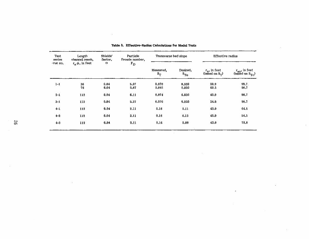
Table 3. Effective-Radius Galculations for Model Tests

Test Length Shields' Particle Transverse bed slope Effective radius series channel reach, factor, Froude number,

-run no~ rctfa, in feet e FD

Measured, Desired, re, in feet reo' in feet ST STo (based on ST) (based on ST

0)

1-1 36 0.04 5.67 0.070 0.030 38.9 90.7 76 0.04 5.67 0.045 0.030 60.5 90.7

2-1 112 0.04 6.11 0.074 0.030 43.0 90.7

3-1 112 0.04 5.27 0.070 0.030 34.0 90.7

4-1 112 0.04 2.11 0.16 0.11 43.0 64.5

4-2 112 0.04 2.11 0.16 0.13 43.0 54.5

N 4-3 112 0.04 2.11 0.16 0.09 43.0 78.8 °'

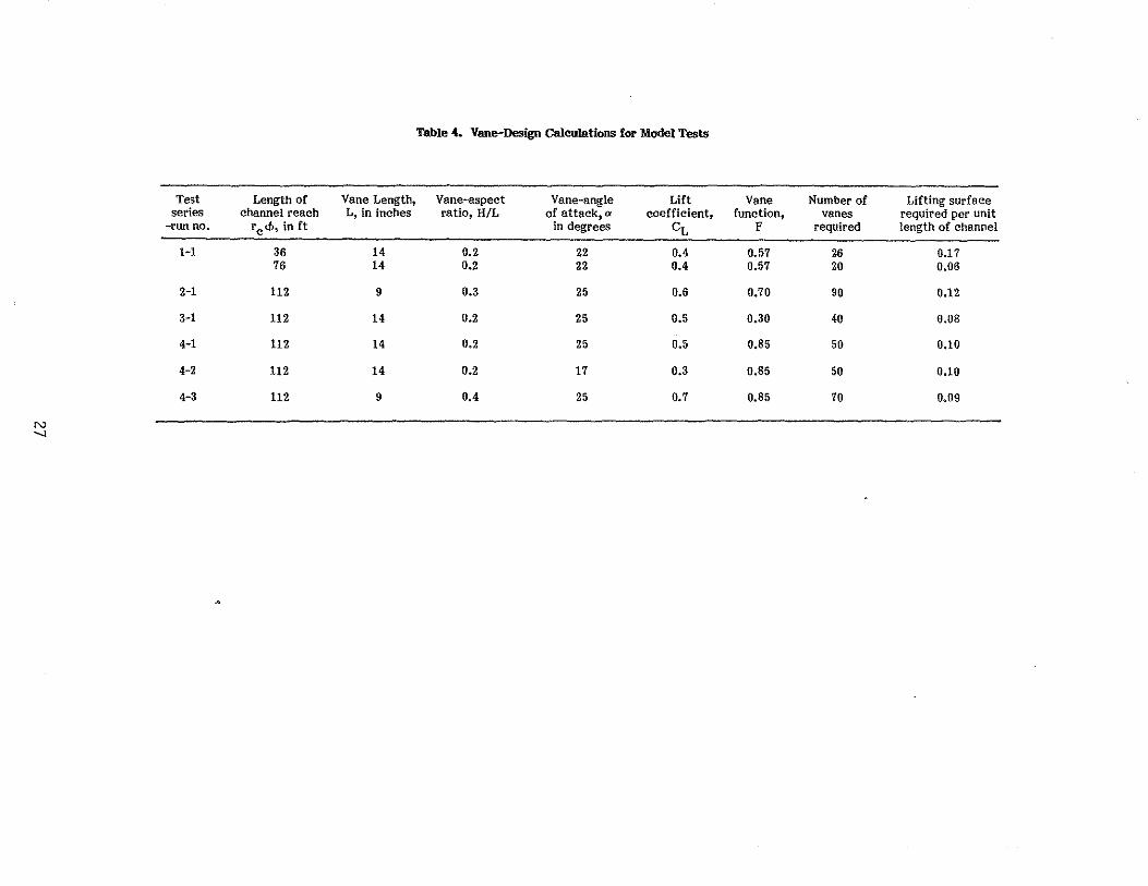
Table 4. Vane-Design Calculations for Model Tests

Test Length of Vane Length, Vane-aspect Vane-angle Lift Vane Number of Lifting surface series channel reach L, in inches ratio, H/L of attack, a coefficient, function, vanes required per unit

-run no~ rc<f,, io ft in degrees CL F required length of channel

1-1 36 14 0.2 22 0.4 0.57 26 0.17 76 14 0.2 22 0.4 0.57 20 0.06

2-1 112 9 0.3 25 0.6 o.7o 90 0.12

3-1 112 14 0.2 25 0.5 0.30 40 0.08

4-1 112 14 0.2 25 0.5 o.85 50 0.10

4-2 112 14 0.2 17 0.3 0.85 50 0.10

4-3 112 9 0.4 25 0.7 0.85 70 0.09

N _,

0 2345678 2345678

0.0 Cl 0 w~ 05 N . - " \. J 0.0 \

0.5

~~-r-.--.-...... ___.,.--~-~-,.~-~---~ /

0.0

0.5

;;/I: l.O :;; h: "'w 15 ~Cl .

2.0

z 1.3 <( 0

~~ 1.2 0 1

::::1 1.1 w,.: :::! ':: l.O _J (J

;;§ '3 0.9 (a)

g:; ~ 0.8 • MEASUREMENT 2 0.7 - THEORY

1.0 _L•-" • • • • • •

1.5

20.

1.3

1.2

l. I

1.0

0.9

0.8

0.7

(b) • MEASUREMENT

-THEORY

0 2345678 01234 DISTANCE FROM LEFT BANK (ft)

5 6 7 8

l.O

1.5

2.0

1.3

1.2

1. 1

1.0

0.9

0.8

0.7

Figure 13. Test Series 1 : Measured Radial Average-Distribution of Depth and Depth-Averaged Mean Velocity Canpared with the Predicted Distributions; (a) Before Installation of Vanes; (b) After Installation of Vanes

.;::

"' ;;:: -' "' ·1 rJ

--- T ----- r 1· ---~--- .:::: 0

<ll' \ ---------I'~ '

Figure 14. Test Series 1 Vane Elnplacanent

28

concept. Between Sections 64 and 100, the average transverse bed

slope was measured to be Sr = 0.070, yielding an effective radius of

38.9 ft. Between Sections 100 and 176 (the end of the bend}, the

transverse bed slope was 0.045, yielding an effective radius of re =

60.5 ft. The "desired" effective radius (that corresponding to Sr0 =

0.030) is reo = 90.7 ft. To meet the objective at minimum lift

surface, the vane height H must be about 333 of the water depth at

the vanes. (Note that because CL decreases when H/L decreases, NHL

is not minimum when F is minimum). As the vanes are placed at a

distance from the channel-center line of 2 to 3 ft, and are to reduce

the water depth there to approximately 0.6 ft, their height should be

H" 0.2 ft, yielding an aspect ratio of approximately 0.2. The near

bed deviation angle is calculated from Eq. 22 (with n = 4.0, d = 0.6

ft, and re= (90.7 + 2.5) ft) to be o "7°, yielding a total angle of

attack of a= 15° + 7° = 22°. According to Fig. 6, the lift

coefficient is then cL" 0.4. The value of F is obtained from Eq. 10

(or Fig. 5) to be F = 0.577 (using n = 4 and H/d = 1/3). The number

of vanes is then readily determined by substitution into Eq. 16: N =

26 between Sect ions 64 and 100; and N = 20 between Sections 100 and

176. Hence, according to this design procedure, a total of 46 vanes

(four more than was actually used) would be required to reduce the

transverse bed slope to 0.03 throughout the channel.

The vanes were i nsta 11 ed in a two-row array up unt i1 Section

104, and a one-row array beyond Section 104. The emplacement of the

two-row array is sketched in Fig. 14. The emplacement of the one-row

array was the same as that of the outer row in Fig. 14. The vanes

were installed on the dry 5.2-cfs channel bed such that their top

edge was 0.4 ft under the 5.2-cfs water surface. The flow rate was

then gently increased to 5.2 cfs, and maintained at this rate for a

period of 160 hours. The bed topography was measured after 10, 20,

40, 80, and 160 hours. The transverse bed slope was observed to

change very rapidly within the first 10 hours after the start of the

flow, as Figs. 15, 16, and 17 indicate. Over the 160-hour period, a

29

.... ., 0.10 t = 0

w ·-.... t = 10 hours Q. / ...... ' . t = 160 hours 0

. ., / .. ,

....l ' •, tf) . ' /' ......... .. ................... \ Cl 0.05 / I" ....... w ,• I ', ro l' I ' w • I ', .--

/ I '.,,,,,.,,,. tf) / ' . er .... I I w I I > 0.00 .. I I'. tf) .. / z <( er BEND I-

20 40 60 80 100 120 140 160 180 200 SECTION NUMBER

Figure 15. Streamwise Variation of Transverse Bed Slope Developnent after Installation ofVanes; Test Series No. 1

30

0

0.0

-"" w 0.2 u ~ 0:

0.4 :::> (ll

~ 0.6 ..J

w m J: I- 0.8 0. w 0

1.0

0

Figure 16.

0.0

w 0.2 u ~ gj 0.4 (/)

:;:: g 0.6 w m

i!= 0.8 a.. w 0

1.0

0

0

2 3 4 5 6 7 8

0.0

t•O t • 10 hours 0.2 t• 160 hours

0.4

;•, .; ' >, 0.6

\,-' •, ., .•. ··· ·._ .... cv···· 0.8

1.0

2 3 4 5 6 7 8 DISTANCE FROM LEFT BANK (fl}

Developnent of Bed Profiles at Section 80 after Installation of Vanes; Test Series No.

2

1•0 t • 10 hours !• 160 hours

2

3

-/ ··.,;

3

1

4

4

5 6 7

........................ r.--...... . -·-- --·, ...... ' / \v1 '•

5 6 7 DISTANCE FROM LEFT SANK (ft}

8

0.0

0.2

0.4

0.6

0.8

1.0

8

Figure 17. Developnent of Bed Profiles at Section 112 after Installation of Vanes; Test Series No. 1

31

tot a 1 of 15. 7 ft3 of sand was moved from the inner half of the

channel to the outer half. In other words, the vane system caused

52% of the sand that was originally moved (during the initial bed

formi ng process) from the outer half to the inner half to return to

the outer half of the channel. As Fig. 13b shows, the average

distributions of depth and velocity are in good agreement with those

predicted by the design procedure. In Fig. 15 it is seen that the

vane system performed better over the first half of the bend than

over the second half. This may have been due to the fact that the

reach between Sect i ans fi4 and 104 was furnished with 28 vanes (in

double-array) whereas the remaining part of the bend had only 14

vanes (in single array), or 30 percent fewer vanes than called for by

the design calculations (which were done after the completion of the

tests).

Table 5 summarizes the overall effectiveness of the vane system

tested in terms of recovery of: (1) Sediment volume in outer half of

channel (the percentage returned to the outer half of the channel of

the sediment vo 1 ume that was ori gi na lly moved from the outer half to

the inner half); (2) near-bank depth (the reduction of near-bank

depth in percent of the reduction required for a chi evi ng uniform

depth); and (3) near-bank velocity (the reduction in near-bank

velocity in percent of the reduction required for the achievement of

uniform velocity). The numbers in parentheses are the recovery

percentages computed by the theory on the basis of the number of

vanes employed. If these numbers equa 1 the actual recovery

percentage, the vane system performed exactly as computed.

numbers in parenthesis are sma 11 er than the actual

percentage, the vane system performed better than computed.

If the

recovery

Table 5

al so shows the reduction of the 1 ongi tu di na l slope of the water

surface caused by the vane system. In Test Seri es 1, the slope was

reduced by 10 percent. The objective is to design the vane system

such that the change in slope is as small as possible (a local

reduction of slope will cause an increase of slope and degradation

downstream).

32

Table S.. Summary of Experimental R1esolts or Vane Tests

Test Vane Vane Vane Number Effectiveness of Vane System -run no. type length, angle, of

in inches .. .. ' lll

vanes degrees

Recovery of Re:covery of Recover of near- Reduction of Number of sediment volume near-·bank depth, bank velocity, slope of vanes with in outer half of i1':percent in percent water surface, significant

channel, in percent in percent scour, in percent

1-11 sheet 14 15 42 52 (52) 63 (53) 58 (61) 10 9 metal

2-1 sheet 9 12*) 84 49 (58) 63 (62) so (70) <.S 6

w metal w

3-1 sheet 14 15 42 44 (47) 36 (SO) 50 (61) 10 7 metal

4-1 sheet 14 15 49 50 (29) 74 (29) 93 12 4 metal

4-2 sheet 14 8 49 44 (19) 62 (17) 100 5 0 metal

4-3 sheet 9 15 70 47 (41) 66 (44) Not <5 6 metal measured

5-1 rock**) 28 15 12***) 30 (58#) zz (50.fl) !00 {80#) Zl ZS

•) slightly curved vanes ••) several unsuccessful, exploratory tests with rock vanes preceded Run 5-1

***) th~ nrockn vanes were installed between Sections 7Z and 112; remaining part of bend was furnished with curved .sheet metal vanes in the Run Z-1 configuration ii Recovery by sheet metal vanes between Sections 72 and 112 in Run 2-1 configuration

In the test series described above, Test Series 1, the side

walls of the flume were of smooth plywood with a roughness much lower

than that of the sand bed. The roughness of real river banks is

often higher than that of the st reambed (due to vegetation, fa 11 en

trees, rip-rap, etc.). In view of that, two test series (Nos. 2 and

4) were al so conducted with roughened side wa 11 s. The roughness

elements were 20-in. long, 1/2-in. wide, 1/4-in. thick pieces of wood

which were nailed onto the side walls 1.5 in. center to center.

Test Series No. 2 was conducted with the same grade of sediment

in the flume as Test Series No. 1. The maximum flow rate was 6.0

cfs. At fully developed fl ow and bed topography, the l ongitudi na l

slope of the water surface and the cross-sectional average values of

depth and velocity were 0.00146, 0.54 ft, and 1.40 ft/sec,

respectively. Thus, Fo = 6,11, n = 3.5, u* = 0,16 ft/sec,

and e ~ 0.04. Based on these flow data, Eq. 12 predicts a transverse

bed slope of Sr = 0.074, which is in good agreement with those measured (Fig. 18a).

In Test Series No. 2, the vane-design formula was tested with a

system of 84 9-in. long, slightly curved vanes (Fig, 19). These

tests were conducted specifically to verify that the lift force, and

therefore the torque Tv• produced by a given lift-surface area

increases when the aspect ratio increases. As the design

calculations, summarized in Tables 3 and 4, show, the number N = 84

corresponds with the design objective of obtaining a reduction of the

transverse bed slope to approximately 0.03, the same objective as in

Test Series No. 1. By reducing the vane length from 14 in. to 9 in.,

the aspect ratio goes up from 0.2 to 0.3, and, according to Fig. 6,

the lift coefficient becomes 0.6 as opposed to 0.4 with 14-in.

vanes. Hence, with 9-in. vanes, the required lifting surface is 333

lower than if 14-in. vanes were used. The calculations summarized in

Table 5 show that the effectiveness of the 9-in. vane system is as

good as that of the 14-i n. system as far as recovery of sediment

volume, near-bank depth and near-bank velocity are concerned. The 9-

34

0 2 3 4 5 6 7 8 0 2 3 4 5 6 7 8 r

0.0

\ ) 0.0

\~ 7 00

0 0 0.5 0.5 ~~ 0.5

--, "" • • • • • <( :i 1.0 1.0 • •••••• 1.0 ;;; f-a: 0.. 1.5 1.5 1.5 0W zO

2.0 20 2.0

1.3 • 1.3 1.3 z ~1~

0

l.2 1.2 1.2 ' 21~ 11 I. I 1.1 0)-" '

• ~t: l.O 1.0 1.0 -u <1 g 0.9 (a) 0.9 (b) 0.9 2w gj > 0.8 • MEASUREMENT 0.8 • MEASUREMENT 0.8

• z 0.7 - THEORY 0.7 -THEORY 0.7

0 2 3 4 5 6 7 8 0 I 2 3 4 5 6 7 8 DISTANCE FROM LEFT BANK (ft)

Figure 18. Test Series 2: Measured Radial Average-Distributions of Depth and Depth-Averaged Mean Velocity Canpared with the Predicted Distributions; (a) Before Installation of Vanes; (b) After Installation of Vanes

-:::: -i<l i<l ;::: <'.i ,,., ,,.,.

:_ : T= r- ,7 ' ..- -------------=- f---_/ -'~"~ . !J

Figure 19. Test Series 2 Vane and Vane Elnplacanents

35

in. vane system is seen to have caused less change in water-surface

slope than the 14-in. system. Therefore, overall the 9-in. vane

system is judged to be more efficient than the 14-in. vane system.

2. Nonuniform Bed Sediment - In Test Series No. 3, the sediment

was sand wiU1 a log normal grain-size distribution with a median

diameter of 0.90 mm and a geometric standard deviation of 1.90 (Fig.

20}. The discharge was 5.8 cfs. Initially, the sand was distributed

uniformly throughout the flume. As the water-sediment mixture was

then propelled through the flume, grain sorting took place. The

smaller fractions tended to accumulate near the inside of the bend

leaving the larger fractions along the outside. When steady-state

conditions were obtained, water-surface elevations, and distributions

of depth, velocity, and grain size, were measured. Notable features

of the bed topography were a point bar along the inner bank between

Sections 88 and 104; and an attendant re 1 at i ve ly deep scour hole at

Section 80. Deep scour holes occurred also at the outer bend at

Sections 136 and 170. It is noteworthy also that the sediment in the

surface layer of the bed was generally finer than that below the

surface. The coarser fractions only surfaced within a distance of

about 2 ft from the outer flume wall. Bed-material samples taken

below the surface of the bed throughout the bend showed that the

original sand mixture was found at a depth of three to five inches

below the bed surface, indicating that grain sorting was limited to

the upper three to five inches of the sediment layer. Bed armoring

did not occur. The overall median diameter of the sediment in the

surface 1 ayer of the bed was determined to be Da = 0 .50 mm. The longitudinal slope of the water surface, and cross-sectional average

values of depth and mean velocity were measured to be 0.00063, 0.47

ft, and 1.56 ft/sec, respectively, yielding F0 = 5.27, n = 6.5, u* =

0.10 ft/sec, and e ~ = 0.04. Based on these flow data, Eq. 12

predicts a transverse bed slope of ST = 0.055, which is in reasonable agreement with those measured (Fig. 21}. The overall average

transverse bed slope was measured to be 0.07.

36

99.5 99 98

w !:::! 95 (/)

0 90 w I-j 80 -~ 70 z 60 <t 50 :c I- 40

8J 30 z LL. 20 I-z 10 w u 0::: 5 w 0...

2 1

0.5 0.1 0.2 0.5 1.0 2.0


Figure 20. Grain-Size Distribution for Nonuniform Bed Sediment; Test Series No. 3

37

5.0

0 2 3 4 5 6 7 8 0 2 3 4 5 6 7 8

0.0 0.0 0 0 \ I \, .. J ~~ 0.5 0.5 _,,

I ! Jt-

;J :i LO 1.0 ••• . •• ::;; I-Q'. a.

1.5 • 1.5 oW zO 2.0 2.0

z 1.3 1.3 ~,~o 1.2 1.2

::;; ·~ 1 1 11 0)-'" .

~ t:: 1.0 1.0 -u ..Jo 0.9 <! ...J 0.9 (a) ::;; w gj> 0.8 . MEASUREMENT 0.8 . MEASUREMENT z 0.7 -THEORY 0.7 -THEORY

0 2 3 4 5 6 7 8 0 2 3 4 5 6 7 8 DISTANCE FROM LEFT SANK (ft)

Figure 21. Test Series 3: Measured Radial Average-Distributions of Depth and Depth-Averaged Mean Velocity Ccmpared with the Predicted Distributions: (a) Before Installation of Vanes; (b) After Installation of Vanes

38

0.0

0.5

1.0

1.5

20

1.3

1.2

1.1

1.0

0.9

0.8

0.7

The vane-design formula was tested with a system of 42 14-in.

vanes in the Fig. 14 configuration. The design calculations (Tables

3 and 4) show that this system corresponds with the design objective

of obtaining a reduction of the transverse bed slope from 0.07 to

0.03, which is seen to be in very good agreement with that

measured. The vane system is seen to have performed with about the

same efficiency as in the case of uniform sand (Table 5),

B. Vanes in Armored Channel

A series of tests was designed specifically to investigate the

vanes' performance in a channel bend with bed armoring. Data from

many river bends in the United States, including Iowa, show that some

areas of the bends are often heavily armored along some reaches, and

raise the question of whether the submerged vanes can achieve

rework 1 ng of the armored portions of the beds that is required to

achieve a flow that is uniform laterally.

The bed material in this test series was that of Test Series ~o.

3 supplemented with coarse sand to give the grain-size distribution

shown in Fig. 22 (several different mixtures were tested before one

was found that armored over a significant part of the bend). During

the process of bed armoring, the bed level was observed to increase

in the straight approach section causing the overall longitudinal bed

slope to be somewhat larger than the slope of the water surface.

Grain sorting took place both laterally and longitudinally. The bed

became fully armored in the entire approach section and in the

beginning of the bend up till Section 88. Between Sections 88 and

172 the bed material near the outer bank was coarse sand with a

median diameter of about 3.2 mm and a geometric standard deviation of

less than 1.4. Armoring occurred over most of the point bar within a

distance of 4 to 5 ft from the inner flume wall. At full

deve 1 opment, the over a 11 average di stri but ions of depth, ve 1 ocity,

and median-grain size were as shown in Fig. 23a, As was expected,

Eq. 12 could not predict the transverse bed slope in this case. So

39

99.5 99 98

w N (/)

95

0 90 w !;:[

80 u 0 70 z z 60 <( 50 I I- 40 a:: w 30 z lJ.. 20 I-z 10 w u a:: 5 w a..

2 1

0.5 0.1 0.2 0.5 1.0 2.0


:Figure 22. Grain-Size Distributions for Nonunifonn Bed Sediment; Test Series No. 4

40

5.0

0 2 3 4 5 6 7 8 0 2 3 4 5 6 7

0.0 0.0

\ 0 0.5 0.5 w

'::::!Io _J f- -0 1.0 1.0 <ta._'- _,.6'•• :;; w -0 r

.~ .. --.~~! -· a:: Cl 1.5 1.5 0 .~· ...-:;:X:: ... 15 ° z ~a'=8o 2.0 2.0 0, .,I

r1 Wu

1.1 ____ ............

~9 ti l.l <iw~ to •..

1.0 ··· ........ ~>1::1 g§~ 0.9 0.9 ·•· ............ Z\lj 0.8 0.8 .......

~w "t rt N!::! 1.0 :J (I) 00 1.0

~ ~ <!'' :;; ;!';Cl 0.5

(a) 0.5 (b) "' <! ~ffi 0.0 • MEASUREMENT 0.0 -·- PREDICTED

~~?;0 }MEASURED

0 2 3 4 5 6 7 8 0 1 2 3 4 5 6 7 DISTANCE FROM LEFT BANK (ft)

Figure 23. Test Series No. 4: Radial Average-Distributions of Depth, Depth-Averaged Mean Velocity, and Median-Grain Diameter; (a) Before Installation of Vanes; (b) After Installation of Vanes

~

~ ff)

I J r -_ - - -r_ ; .\- ------- T 1·;:: --- ----- 0 Q:J

[--1 6 ft

~ -I

Figure 24. Test Series No. 4 Run 3 Vane Nnplacenent

41

8

0.0 ) 0.5

1.0

1.5

2.0

r 1. 1

1.0

0.4

0.8

r 1.0

0.5

0.0

8

far, no mathematical model has been developed that can predict the

bed topography in a partially armored river bend. However, the bed

profile is formed by the secondary-fl ow component so the transverse

bed slope must correlate with the balance between the radial

components of the bed-shear stress and weight of some representative

bed particle, or group of bed particles. Therefore, it is reasonable

to expect that the parameter conste 11 at ion of Eq. 12 still applies,

and that an acceptable design relation can be obtained by using Eq.

12 with a calibration factor, which obviously must be site

specific. With a particle Froude number based on D = 2.7 mm, and e = 0.04, the calibration factor becomes 7.0.

The test series included experiments with two different vane

lengths (L) and two different vanes angles (a'). In Run 4-1, the

performance of 49 14-in. vanes, installed at angle a' = 15°, were

tested; in Run 4-2, the same 49 14-in, vanes were tested with a' = 8°. The vane emplacement was as shown in Fig. 14. The system of 49

14-in. vanes at a' = 15° corresponds with the design objective of

obtaining a reduction of the transverse bed slope from 0.16 to 0,11;

the system of 49 14-in. vanes at a' = 8° corresponds with the design

objective to reduce the transverse bed slope from 0.16 to 0,13. A

major objective of these two experiments was to verify that the

performance of the vane system is sensitive to a', in agreement with

the theory. As Fig. 23b shows, the 15-degree system performed

slightly better than the 8-degree system, as predicted, In both

cases, the vane system performed better than the design calculations

predicted in terms of recovery of near-bank depth and velocity. This

may have been due to the fact that the calculations (and the

analysis) re 1 ates to the entire channe 1 cross sect ion, whereas the

vanes, by their positioning, affected the flow in mainly the outer

half of ~he channel. Because of armoring, the vanes were not able to

move any major amounts of sand away from the inner half of the

channel. It is important to note that the 7-degree difference in

vane angle had only little effect on the overall performance.

42

In Run 4-3, the performance of 70 9-in. long vanes, installed at

an angle of a' = 15° in the Fig. 24 configuration, were tested. The

objective was the same as that of Run 2-1 with uniform sand; i.e., to

verify that the efficiency of a system with given 1 Ht-surface area

increases when the aspect ratio of each i ndi vi dua 1 vane increases.

As the design calculations, summarized in Tables 3 and 4, show, the

system of 70 9-in. long vanes at a:' = 15° corresponds with the design

objective of obtaining a reduction of the transverse bed slope from

0.16 to 0.09. The predicted improvement over the 14-in. vane system

is not apparent from the test results (Fig. 25); in fact, the

performance is seen to have been slightly lower than that of the 14-

in. system as far as near-bank depth recovery is concerned. However,

it is noteworthy that the lift surface of the 9-i n. system was about

10% smaller than that of the 14-in. system, and that the 9-in. system

did not produce any measureab le change of the slope of the water

surf ace.

At the con cl us ion of each of the aforementioned runs, the vane

system, and the bed topography developed by the vane system, were

subjected to a lower flow rate of the order of 3.5 to 4.0 cfs. In no

case did the lower flow rate cause any significant change in the bed

topography developed at the higher flow rate.

c. Rock Vanes

A number of experiments were carried out with "vanes" composed

of windrows of gravel and marbles (scaled-size rock) in an attempt to

develop an economi ca 1 a 1 ternat i ve to sheet-pile vanes. The

experiments, which are sti 11 ongoing, have not produced any

encouraging results so far. One of the major problems is the

embedment of the vanes. As the flow passes over the windrows, near

bed turbulence generates scour holes in the bed at the bottom of the

windrows. As a result, the windrows tend to settle, usually in an

uneven manner, and collapse.

43

0 2 3 4 5 6 7 8 0 2 3 4 5 6 7

0.0 0.0

\ 0 0 0.5 ~~ 0.5 _,, _, .

LO l.O <( :r: ::;;t-"' "- 1.5 1.5 0W zO -·--· 49 14-INCH VANES} ~ 15•

2.0 • MEASUREMENT 2.0 - 70 9-INCH VANES a -L.

0 2 3 4 5 6 7 8 0 1 2 3 4 5 6 7 DISTANCE FROM LEFT SANK (ft)

.Figure 25. Test Series No. 4: Radial Average-Distributions of Depth; (a) Before Installation of Vanes; (b) After Installation of Vanes

8

)

8

0 2 3 4 5 6 7 8 0 2345678

0.0

0.5

1.0

1.5

2.0

~~o~:~\ ~~ wl \

Ji~~~\ l'v r \ ] 1.5 [

/10.0

0.5

110 o"' 1.5 zO

2.0

z 1.3 ;:}~c l.2 ::;;p 11 o,..: . ~'::: LO :::; u <(g 09 ::;;w @',> 08 z 0.7

(a)

• MEASUREMENT

2.0

1.3

1.2

I.I

1.0

0.9

0.8

0.7

(b)

----· 9-INCH VANES - ROCK VANES

0 2345678 012345678 DISTANCE FROM LEFT BANK (ft)

Figure 26. Test Series No. 5: Radial Average-Distributions of Depth, and Depth-Averaged Mean Velocity between Sections 72 and 112; (a) Before Installation of Vanes; (b) After Installation of Vanes

44

rs 2.0

1.3

1.2

LI

l.O

09

08

0.7

The most encouraging result was obtained in an experiment in

which 12 24-in. long windrows of marble-filled baskets were installed

between Sections 72 and 112 at 15° with the mean-flow direction (Fig.

27), with the remaining part of the bend furnished with 40 9-in.

sheet-metal vanes in the Fig. 19 configuration. The bed sediment was

that used in Test Series No. 2. The marble vanes were installed on

the Run 2-1 channel bed, as developed by the 84 9-i n. vanes, by

replacing the 9-in. vanes between Sections 72 and 112 with marble

vanes. Fig. 26 shows the average distributions of depth and velocity

between Sections 72 and 112 before any vanes were installed (Fig.

26a); a.fter the 9-in. vanes were installed (dotted curves in Fig.

26b); and after the 9-in. vanes were replaced by the marble vanes

(solid curves in Fig. 26b). Approximately 50% of the sand that the

9-in. vanes recovered in the outer half of this channel portion was

lost again when the 9-in vanes were replaced by the marble vanes.

The marble vanes reduced the near-bank velocity to the cross

sectional average value for this portion of the bend, as indicated in

Fig. 26b; however, this reduction was accompanied (and explained) by

a very significant decrease of the slope of the water surface over

this reach. Despite that this experiment was by far the most

successful of the rock-vane experiments, Fig. 28 cl early show that

more development work is needed before "rock vanes" can be considered

to be an efficient alternative to sheet-pile vanes.

D. Discussion of Results

Al 1 tests were conducted with a vane angle of a' = 15 degrees

with the exception of Runs 2-1 and 4-2 in which the angle was 12 and

8 degrees, respectively.

15 degrees was at the

It was very clear from the tests that a' = upper limit of the workable a' -range.

Objectionable scour always occured at a few of the vanes, even

at a' = 12 degrees, although this was not reflected in the "recovery"

efficiencies. However, no scour occurred when a' was 8 degrees.

As 6 was always of the same order of magnitude (approximately 10

45

Figure 27. Test Series No. 5 : Rock Vanes before Admission of Flow

Figure 28. Test Series No. 5: Rock Vanes after Adnission of Flow

46

degrees) it would appear that the optimum angle of attack,"• is of

the order of 20 degrees. (a = the angle at which the bottom current

approaches the vane).

The curving of the vanes in Run 2-1 was done in the belief that

the 1 ift and drag characteristics would be improved. Separate tests

with straight and curved vanes in one of IIHR's straight, rigid-bed

flumes showed that fl ow separation was less severe when the vanes

were curved. As Table 5 shows, the efficiency of the curved-vane

system was very good, in particular· considereing that there was no

measurable reduction of the longitudinal slope of the water

surface. However, objectionable scour was observed at a few of the

vanes. This might not have happened if the vanes had been slightly

less curved.

Throughout the study the performance of the various vane systems

was checked al so by observations of the behavior of surface fl oats.

Fl oats re 1 eased at the center 1 i ne of the channel should be carried

sidewards toward the outside at a rate that can be calculated from

the transverse bed slope that the vane system is designed to achieve

(Odgaard, 1984). The float technique was used also, together with

dye injections, to study the flow behavior around each individual

vane. These tests led to the conclusion that the length of the vanes

and their lateral spacing should not be more than about twice the

water depth. If the length of the vanes or their 1 atera l spacing, or

both, exceeded twice the water depth the vanes tended to generate two

(or more) secondary flow cells downstream rather than one, which

obviously would reduce the overall performance of the vane system.

The performance of the various sheet metal vanes is illustrated

on the photographs in Figs. 29 through 36. Fig. 29 shows a naturally

formed bed topography with partial armoring (from Test Series No.

4). Notable features are the flat point bar and the steep slope at

the edge of it. Fig. 29 also shows the 14-in vanes installed in a

two-row array up to Section 98 (at the top of the picture) and a one-

47

Figure 29. Naturally Formed Bed Topography in Test Series No. 4 (Looking Upstream)

Figure 30. Bed Topography in Test Series No. 4 (Looking Upstream) after Installation of 14-in. Vanes

48

Figure 31. Depth Distribution at Section 112 in Test Series No. 4 Before Installation of Vanes

Figure 32. Depth Distribution at Section 112 in Test Series No. 4 After Installation of 14-in Vanes

49

Figure 33·J Close-up of Bed with 14-in. Vanes(one barely visible) at Section 112 in Test Series No. 4

Figure 34. Bed Topography IX:>wnstream fran Section 112 in Test Series No. 4 with 14-in Vanes

50

Fgiure 35. Depth Distribution at Section 112 in Test Series No. 4 After Installation of 9-in. Vanes

Figure 36. Depth Distribution at Section 112 in Test Series No. 2 After Installation of 9-in. Vanes

51

row array over the rest of the bend. The two-row array was later

extended up to Section 112 (at the lower edge of Fig. 29), After 160

hours with a discharge of 5.8 cfs through the flume, most of the

point bar had disappeared (Fig. 30). Note in Fig. 30 that some of

the vanes in the outer row had become comp 1 ete ly covered with sand.

The depth distribution at Section 112 is indicated in Figs. 31

(before installation of vanes) and 32 (after installation of

vanes). For visualization, a string was extended horizontally at the

water level, and 5 thin staffs with 1/10-ft marks were driven into

the sand bed (after draining of the flume) at 1 ft intervals. The

outer staff was 2 ft from the outer flume wall. The depth at this

staff is seen to have been 0.8 ft before vanes were installed. After

the vanes were installed the depth here was reduced to 0.4 ft (Figs.

32 and 33). Downstream from 112, where only one row of vanes were

installed, the result was also very satisfactory, as Fig. 34 clearly

shows. The bed recovery at Section 112 with 9-in. vanes is shown in

Figs. 35. (Test Series No. 4-3) and 36 (Test Series No. 2-1).

IV. VANE DESIGN FOR EAST NISHNABOTNA RIVER BEND

The results of the theoretical analysis and the laboratory-model

experiments were used for the design of a vane structure for the

meander bend in Fig. 3 for the protection of U.S. Highway 34 and its

bridge over East Nishnabotna River. The flume in which the

aforementioned experiments were conducted, models, with some

idealization, this meander bend at an undistorted scale of

approximately 1: 10. Fig. 37 shows the IIHR flume overlaid the

prototype bend, using the scale ratio 1:10.

A. Field Surveys

Cross sections of the river bend (of which a plan view is shown

in Fig. 38) were surveyed October 6-7, 1983 (eight cross sections),

and April 30 through May 2, 1984 (ten cross sections) to define the

channel geometry at two different times for two different flow rates

52

PROTOTYPE SCALE (FT)

0 200 400

t N

I

U.S. HIGHWAY 34

Figure 37. Plan-View of IIHR's Sediment Flume overlaid the East Nishnabotna River Bend at Red Oak, Using a Scale Ratio of 1:10

53

NOTE' COORDINATES OF REFERENCE REFERENCE POINT R IS AT NORTH

WEST WING OF BRIDGE, DOT STATION 421, J!il FT NORTH OF HIGHWAY CENTER LINE.

POINTS (APPROXIMATE)

POINT WEST (FT)

R 0 A -90 B 45 c 245 D 430 E 610 F 740 G 690 H 320 I -125 J -360

BANK, MAY 1, 1984

U.S. HIGHWAY 34

NORTH (FT)

0 85 160 165 175 250 510 870

1,080 1,240 1,300

0 200 400

N

2 0 i= &l "'

0' ' ' -f--180'+200'---!-:. ' ' ' 230,

D C B 0 !!!

R

600

\ -(.\0~

s'<-c

STEEL JETTY

Figure 38. Plan-View Sketch of the East Nishnabotna River Bend at Red Oak, Iowa

54

(Figs. 39 and 40). Also, detailed velocity measurements and bed

materi al samples were taken at each cross section to determine the

variations in the velocity profiles and the size of the bed

sediment. The velocity was measured over 5-6 verticals across each

section using a 5-in. Ott current meter. In each vertical, the

velocity, u, was measured in five points; the recording time was 30-

40 seconds at each point. Based on these measurements, a depth

averaged velocity, u, was determined for each vertical. The cross

sect i ona l average velocity, ua, was determined by di vi ding the fl ow

rate (obtained by integrating the velocity distribution) by the

measured cross-sectiooal area. The bed samples were taken by a grab

bucket sampler which samples to a depth of 5-6 in. below the bed

surface. The samples were dried, weighed, and sieved for size-

distribution analysis.

The data are summarized in Tables 6 and 7 and in Fig. 41. The

sections are indentified by their distance from the northern

guardrail of the bridge. The distances are along the May 1, 1984,

channe 1-center 1 i ne. The elevations are 1 i sted in re 1 at ion to mean

sea level using the stage-discharge relation for the U.S.G.S. gage at

Coolbaugh Street bridge in Red Oak (Fig. 42), which is 6,000 ft

downstream from the Highway 34 bridge. The datum of this gage is

1005,45 ft above mean sea level. The longitudinal slope of the water

surface was measured to be 0.00064 and 0.00066, respectively, in the

two surveys. [Note: The Iowa State Highway Commission Bench Mark on

the south east wing of the bridge (Station 425+42, 19 ft south of the

highway center line) is not tied in with the U.S.G.S. gage at

Coolbaugh Street bridge. This was verified by the Office of Bridge

Design, Iowa Department of Transportation. Based on the U.S.G.s.

gage at Coolbaugh Street, the bench mark is at elevation 1043.58 ft

(or 2.97 ft above that indicated on the bench mark)]. The n-values

( characterizing the channel resistance) are ca 1 cul ated by the Darcy

Wei sbach relation, using measured values of ua, S and da: n =

na = KUa/lgSda· Al 1 grain-size distributions for the bed and bank

55

Figure 39. East Nishnabotna River on May 2, 1984, I.Daking Upstream fran the U.S. Highway 34 Bridge

Figure 40. Survey at Section 4, May 2, 1984

56

Table 6. High-Flow Data from East Nislmabotna River Bend

Section Distance Flow rate, Cross-s'ectional Surface Elevation Cross-sectional Cross-sectional Cross-sectional number from in cubic area, in width of of water surface, average velocity, average depth average velocity

bridge, in feet per squar-e feet channel, b, in feet above ua, in feet d8, in feet profile exponent feet*) second in feet mean sea level per second na

l 120 5,390 1,960 193 1022.4 2.75 10.2 2.4

2 350 4,740 1,360 130 1021.9 3.49 10.5 3.0

3 550 4,370 1,030 135 1021.5 4.24 7.6 4.3

4 730 4,110 990 120 1021.3 4.15 8.3 4.0

(J1 5 900 4,430 1,130 170 1021.8 3.92 6.6 4.3 .__, 6 1,160 4,620 1,030 170 1022.l 4.49 6.1 5.1

7 1,510 3,810 910 162 1021.5 4.18 5.6 4.9

8 l,960 3,490 900 178 1021.3 3.88 5.1 4.8

9 2,470 3,470 760 185 1021.6 4.57 4.1 6.3

10 2,710 3,600 850 188 1021.9 4.24 4.5 5.6

*) Distance from northern guardrail of bridge, measured along the May 1, 1984, channel-center line

Table 7. Low-Flow Data from East Nishnabotna River Bend

Section Distance Flow rate, Cross-sectional Surface Elevation Cross-seetione.l _Cross-sectional Cross-sectional number from in cubic area, in width of of water surface average velocity, average depth average velocity

bridge, in feet per square feet channel, b, in feet above u8 , in feet da, in feet profile exponent feet*) second in feet mean sea level per second "a

2 350 118 83 108 1014.3 1.42 0.77 4.5

3 550 118 81 100 1014.4 1.46 0.81 4.5

4 730 118 78 90 1014.5 1.51 0.87 4.5

5 900 118 92 120 1014.6 1.28 0.77 4.1

6 1,160 118 73 116 1014.8 1.62 0.63 5.7

7 <.n

1,510 118 83 93 1015.0 1.42 0.89 4.2

00 8 1,960 109 85 93 1015.3 1.28 0.91 3.7

10 2,710 109 60 64 1015.8 1.82 0.94 5.2

*)Distance from northern guardrail of bridge, measured along the May 1, 1984, channel-center line

s 1022

~ 1020 ::; 1018 w > 1016 0 ~ 1014

z 1012 Q !;; 1010

GJ 1008

ci 1006

""

~ 081 g 2 ~ 4 ~ 10 w 50 w

"' ~

S'1022

~ 1020 w 1018 > 0

1016 CD <(

z 1014 0 1012 >== §! 1010 w ci 1008

~ 1022

~ 1020

~ 1018

&5 1016

<( 1014 z Q 1012 I-§! 1010

~ 1008

0 20 40 60 80 100 120 140 160 180 200

EL1022.4

P' 10 50

1.6 0.7 3.6 2.8 4.1

DEPTH-AVERAGED MEAN VELOCITIES (fps)

SECTION I '.------=-::::..:'.'. __ EL 1007.2

0 20 40 60 80 100 120 140 160 180 200

DISTANCE FROM LEFT BANK (ft)

0 20 40 60 80 100 120 140

~ l1..-w EL. 1021.9

~"'I .,,.

2.6 4.5 5.0 3.4 p I. I 3.7

Cl 2 DEPTH-AVERAGED

:::l 4 MEAN VELOCITIES (fps)

\<! 10 10 w 50

9.t ~{giii'Wii'"'A'WA•-&~oo~~F~·w~ 50 w

"' ;:: (f)

SECTION 2 ____ _§:_L_JQ08.4

Cl 2 ~ 081 :::l 4 \<! 10 w 50 w "' ;:: (f)

0

0

20 40 60 80 100 120 140


20 40 60 80 100 120 140

EL. 1021.5 2.9 3.4 3.9 4.3 5.2 4.8


EL. 1014.4 ...... ~k, . .,....,. ~':;=•='-=-...,.:.'Z~~~w.».1r.m~~

.:~\::'?it§:, <':ii . ,,,, ... loi 10 50

SECTION 3 __ EL._ 1009.2

0 20 40 60 80 100 120 140


1022

1020

1018

1016

1014

1012

1010

1008

1022

1020

1018

1016

1014

1012

1010

1008

Figure 41. Sections 1 thorugh 10 of the East Nishnabotna River Bend

59

1022

1020

1018

1016

1014

1012

1010

1008

1006

.., ': 1022

~ 1020

w 1018 > g 1016

<( 1014 z Q 1012 t-:g 1010

~ 1008 w

-': 1022

~ 1020

w 1018 > 0 1016 al <( 10.14 z 0 1012

~ 1010

~ 1008 w

£1022

~ 1020

::. 1018 w b 1016

!11 1014

15 1012

Si 1010

G'; 1008 -1 w 1006

~ 08! ;3 2 t:J 4 ~ 10 UJ 50 w C)

;:! <f>

~ ~ w

~ "'! ;3 2 t:J 4 ~ 10 UJ 50 UJ C)

;:! <f>

0

0 20 40 60 80 100 120

EL. 1021.3 ' 2.8 3.2 4.2 4.6 4.6

DEPTH-AVERAGED MEAN VELOCITIES (fps) loi

10 50

SECTION 4 EL. 1007.4

0 20 40 60 80 100 120

DISTANCE FROM LEFT BANK (fl)

20 40 60 80 100 120 140 160 180

EL. 1021.8 2.2

9 2.7 3.7 4.3 4.7 3.5


SECTION 5

0 20 40 60 80 100 120 140 160 180


0 20 40 60 80 100 120 140 160 180

EL 1022.l

3.0 .,,.

4.0 4.5 4.7 5.3 DEPTH-AVERAGED

MEAN VELOCITIES (fps)

EL 1014.8 .. :4~~-&."'lfiID~i@if~.,

1022

1020

1018

1016

1014

1012

1010

1008

1006

r: 10 50

F 10 50

SECTION 6 __ _fkJQ99.4

0 20 40 60 80 100 120 140 160 180 DISTANCE FROM LEFT BANK (ft)

Figure 41. Continued

60

1022

1020

1018

10\6

1014

1012

1010

1008

1022

1020

1018

1016

1014

1012

1010

1008

uJ 1022

~ 1020

6 1018 CD "'1016

15 1014

;:: 1012 :;! 'j 1010 w

_J

~ 1022

g; 1020

al 1018

"' z 1016

Q 1014

~ 1012 w _J w

"" _J (f)

> '°"t g; 1020 0 ~ 1018

z 1016 0

~ 1014

w _J

w

-"" _J

~ 1022f !3'.1020

al 1018

"' 1016 t z Q 1014 f-:;! 1012 w _J w

~ 08! i3 2 w w 4 ~ 10 w w 50

"' f'.' (f)

0 2 i 081 :::J 4 3i 10 w 50 w

"' ;::! (f)

~ !!..-w

~''I 8 2 w 4 ~ 10 w 50 w

"' f'.' (f)

~ !!..-w

~,,I 0 2 :::J 4 3i 10 w 50 w

"' iS (f)

0 20

SECTION 7

0 20

0 20

40 60 80 100 120 140

EL 1021.5 -2.2 3.3 4.1 5.3 4.9 DEPTH-AVE RAGED


·---~- · f~&~~}2,,.,«4!~itr~~, _Elo__ 1_0_12~_ -'"--~

40 60 80 100 120 140


160

160

180

lo! 10

50

180

40 60 80 100 120 140 160 180

1022

1020

1018

1016

1014

1012

1010

3.5 4.2 ~

EL. 1021.3

3.6 4.2 4.7 DEPTH-AVERAGED


3.1

Joi 10 50

1022

1020

1018

1016

1014

1012 SECTION 8

•---"- EL 1015.3 "::.'~~eaoomf1iJfil®JJk4t's=~::1,·w1Hr.:ft~,pr1

El,J_Qlbi?_

0 20 40 60 80 100 120 140 160 180


0 20 40 60 80 100 120 140 160 180

r r,, 5.1 5.5 4.6 1020 DEPTH-AVERAGED

MEAN VELOCITIES (fps) 10 1018

50 1016 SECTION 9

1014

0 20 40 60 80 100 120 140 160 180

DISTANCE FROM LEFT SANK (ft)

0 20 40 60 80 100 120 140 160 180

EL 1021.9 p 102? 34 5.6 - 4.6 3.3 24

1020 DEPTH-AVERAGED MEAN VELOCITIES (fps) 10 1018

50 1016 SECTION 10 1014

1012

0 20 40 60 80 100 120 140 160 180


Figure 41. Continued

61

30 I I

-- ----- --- - -- - ----- ---- --------- -· - - - - -- - - - -- -- - --- - - -l MAXIMUM GAGE HEIGHT ON RECORD' 28.23ft

I

25 I I I I

DATUM OF GAGE IS 1005.45 ft I I

~ ABOVE MEAN SEA LEVEL Cl I - 0:: I ~ 20 0 I

f- u I I

I w I 0:: I

<.9 z I I

w 15 0,,,1

I -· W ul

w (90 I

a:: 0 l <.9 <to I ::::i I •I

<( 10 U 00 I

<.9 (/) !<) I

0 I I I

2 I :::> I

I 2 I 5 x I

I <t I 2

102 5 103 5 104 5 DISCHARGE (cfs)

Figure 42. Rating O.lrve for the U.S.G.S. Water-"'Stage Recorder on East Nishnabotna River at Red Oak (at Cbolbaugh Street Bridge)

62

30

25

20

15

10

5

sediments are shown in Appendix II. Due to high flow velocities, no

samples were taken from the bed of the main channel in the May 1984

survey. Median-grain diameter and geometric standard deviation of

the composite grain-size· distribution for the bed material of the

October 1983 main channel are determined to be 0.45 mm and 2.0,

respectively. There is no indication that bed armoring occurred in

the channel bend.

Fi gs. 41 show the ten cross sections measured in the Apri 1-May

survey with the eight October cross sections superimposed (dotted)

for comparison. (The lateral position of the October cross sections

relative to the April-May sections is only approximate). It is seen

that for most sections the elevation of the bed in the October

channel is very close to that of the average depth in the Apri 1-May

channel. This indicates that the increase in transverse bed slope

due to increase of flow rate is accomplished basically by a tilting

of the October bed about the April-May channel centerline. At

Section 2, the April-May high flow is seen to have caused an overall

lowering of the October 1 ow fl ow channel bed by 5-6 ft. Note al so

that the deepest point in Section 1 (130 ft upstream from the bridge)·

is at elevation 1007.2 ft, which is about 5 ft lower than the stream

bed elevation for which the bridge foundation was designed (Iowa

State Highway Commission, Design No. 262, Montgomery County, File No.

21400, July, 1963). The cause of this overall lowering of the stream

bed may be re 1 ated to the presence of the 600-ft rock protection on

the right bank near the bridge (Fig. 43). According to Jansen et al.

(1979), fixation of an outer bank which is being eroded induces a

steeper slope in the cross section and a greater depth at the toe of

the fixation structure.

B. Design Computations

The design computations are summarized in Table 8. The

transverse bed slopes listed in Table 8 are determined as the slopes

of best-fit lines through the depth points within the central portion

63

Figure 43. East Nishriabotna River on May 2 , 1984, Looking Downstream toward the Highway 34 Bridge (The rock protection is along the right bank in the upper-center portion of the picture)

64

Table 8. Vane Design Compute.tionll for East Nishne.botna River Bend

Section Distance Transverse Particle Effective Deviation Vane angle Vane Rquired Sectional Required Required number from bed slope Froude radius of angle, a with mean function, lifting surface lifting number

bridge ST number, curvature, in flow F surface area of surface, of vanes in feet*) FD rf.' in degrees direction, a' per unit channel, NHL, in (3-ft high,

eet surface . rc4>b, square 12-ft long) area of tn square feet channel feet

3 550 0.09 15.1 l,370 7.1 12.9 0.52 0.0115 25,650 295 8

4 730 0.13 14.8 1,010 9.7 10.3 0.41 0.0135 21,000 284 8

5 900 0.11 14.0 900 9.4 10.6 0.52 0.0153 36,550 559 15

6 1,160 0.11 16.0 950 10.0 10.0 0.40 0.0103 51,850 534 15

7 1,510 0.08 14.9 1,120 7.5 12.5 0.43 0.0086 64,800 557 15

"' (J1 8 1,960 0.04 13.8 1,890 3.9 16.1 0.44 0.0047 40,000 188 5

*) Distance from northern guardrail of bridge, measured along the May 1, 1984, channel-center line

of the cross sections. These slopes are seen to be of the same order

of magnitude as those measured in the laboratory model. However, the

laboratory model is a constant-radius bend following a straight

channel (with radius = infinity). The radius of the river curve

decreases gradually from infinity at the inflection point near

Section 8 to less than 400 ft at Section 5. Between Sections 5 and

3, the radius increases again to infinity. Considering the short

distance over which these changes occur, it is quite obvious that the

bend flow cannot at any point be considered to be fully developed

with depth and velocity distributions as in the downstream reach of a

1 ong, constant-radius bend (for which most bend-fl ow theories are

developed). However, the effective-radius concept can be used for

the vane design. Table 8 lists the effective radii, re, as

calculated by Eq. 12, using e = 0.05; d = da;

ua/,I gD{p s -P )/p ; and the measured va 1 ues of Sr. Fo = =

The laboratory-model tests indicated that the vane-angle of

attack should be of the order of 20 degrees. With a = 20 degrees,

and the near-bed deviation angles, o, calculated by Eq. 23, the

vanes' angle with the mean-fl ow direction is obtained from Eq. 24:

a' = a - o. The a' values are seen to range from 10 to 16

degrees. Considering the uncertainty involved in the determination

of the optimum value of a, there does not appear to be justification

for a greater accuracy on a' than about two to three degrees. In

view of the greater risk of scour at the larger values of a, it would

be advisable to let a' be closer to 10° than 16°.

According to the basic theory the required area of lifting

surface decreases with increasing aspect ratio. However, there is a

practical upper limit to the aspect ratio. For the vanes to be

erosion preventive their height H should be less than half the water

depth at the flow rates at which bank erosion occurs; i.e., whenever the fl ow rate in this river bend is greater than about 1500 cfs. (At

1500 cfs, the near-bank velocity at Section 3 through 6 exceeds 3.5

ft/sec, which is the limiting velocity recommended by the U.S. Bureau

66

of Reclamation for the design of a stable, firm-loam channel carrying

water with colloidal silts.) According to the U.S. Geological

Survey, this flow rate is exceeded on the average (based on 60 years

of records) 4% of the time, or approximately 15 days per year (Fig.

44). The 1500-cfs river stages are obtained from the U.S.G,S stage

discharge relation for the gage in Red Oak using a longitudinal

water-surface slope of 0.00064. The 1500-cfs average water depth is

estimated to be approximately 5 ft. Therefore, the top of the vanes

should be more than 2.5 ft under th!'l 1500-cfs stage to be erosion

preventive at this and higher stages. From Fig. 41 follows that if

the vanes are installed at low flow with their top edge 2.5 ft below

the 1500-cfs stage and can maintain the present low-flow bed profile,

the H/d-value will be optimum (of the order of 0.2-0.3) at the

extreme high flow when most erosion losses would occur. For this

situation to occur, the vane height must be of the order of 3 ft. In

the model, the best performing vane was four times as long as it was

high. A 3-ft high prototype vane should then be 12 ft long. If the

vane is much longer than that it may generate two (or more) secondary

flow cells downstream rather than one, which reduces the overall

performance. Using H/L = 0.3, and a = 20°; the lift coefficient as

given by Fig. 6 is CL= 0.5. The value of F selected for the design

was the

section.

channel,

bed is

vanes.

minimum value, Fmin• corresponding to the n-value for the

The lifting surface per unit surface area of the

NHL/(r q,b), required to maintain a horizontal "low flow" c

then readily calculated, and so is the required number of

Each vane would be acted upon by a maximum lift force of the

order of Fv = l/2clpu 2HL ~ 300 lbf which, when uniformly distributed

over the 36 ft2 1 i ft i ng surf ace would yield a bending moment 3 ft

from the top of the vane of about 450 ft-lb. If the vanes are made

of sheet piles, wood planks, or thin concrete slabs, the drag force

on the vanes would not be a design factor. Although the forces on

the vanes from the fl ow are thus very sma 11 it is recommended that

67

Cl w Cl w w u x

wW 2(1) I-~ ll.. (!) 0 a:: I-<:( Z I WU u (/) a:: -wO Cl. Cl

w I-<:( u Cl z

60

50

40

30

20

10

5

2

0.5

0.2 0.1

102

5.0 5.2 5.6 6.2 GAGE HEIGHT (ft)

5

GAGE HEIGHT (ft) 6.7 70 8.0 9.4 I 1.6

103

DISCHARGE (cfs)

5

Figure 44. Frequency Distribution for Discharge in East Nishnabotna River at Red Oak

68

each vane has at least two of its piles extending down below the top

of the firm shale layer, which, according to the Iowa State Highway

Commission Design No. 262 (File No. 21400, July lg63) is at elevation

1004 ft (sounding dated July 31, 1962). The support piles should

thus be at least 15 ft long, and preferably 18 to 20 ft.

The positioning of the vanes on the stream-bed requires careful

planning. In order that the vane system as a whole function at

optimum efficiency, the longitudinal and lateral spacing of the vanes

must be such that a single-cell circulation is induced in the flow

section. If the vanes are spaced too far apart laterally, two or

more secondary flow cells are induced. Dye and float studies in the

laboratory model indicated that the lateral di stance between two

vanes should be less than or equal to two times the water depth. The

optimum distance, which undoubtedly is a function of L and a, was not

identified in the model studies. Satisfactory results were obtained

in the mode 1 with a 1atera1 vane di stance of two times the water

depth. Based on a 4,000 cfs river flow, the prototype vanes should

then be spaced about 12 ft apart in the lateral direction. The

proposed emplacement of the vanes is detailed in Fig. 45, and

Table 9,

The above emplacement applies to the reach between Sections 2

and 9. However, it is equally important that measures be taken to

guide the fl ow through the bridge section. The effective width of

the channel at the bridge section is presently less than half the

width for which the bridge was designed. There is obviously a need

for measures that can: (1) Turn the river flow southward (90°) over a

short distance (less than 300 ft) without endangering the left bridge

abutment; and ( 2) gene.rate a widening of the effective channel width

at the bridge section. It is uncertain to what extent Iowa Vanes can

accomplish such a task. The most logical solution would be to use a

combination of bank rip rap and vanes as sketched in Fig. 46. Note

that bank rip rap alone would not produce a widening of the river

channel.

69

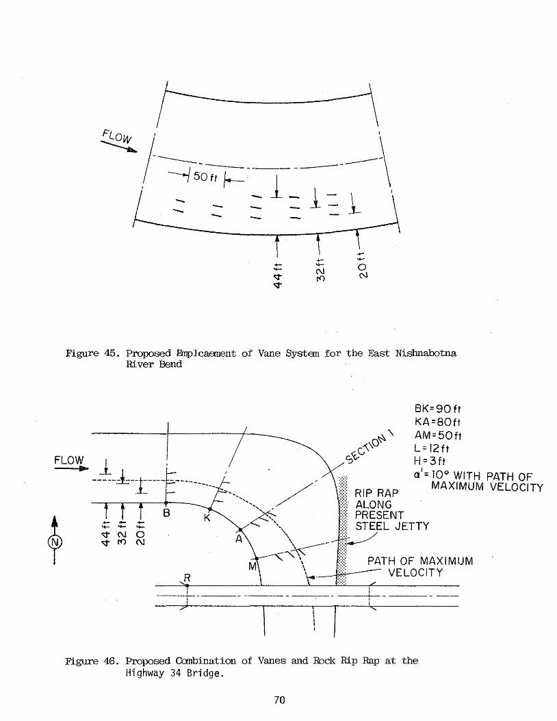
~1·--- --·\ , --/ 50tt 1--- l

:: =l _l ' ---- --

Figure 45. Proposed Elnplcaement of Vane System for the East Nishnabotna River Bend

FLOW .. l ' -----±--t----- ----------- ,

j --. - .........

- - -............ <:t (\J 0 <:t I") (\J

B

R

K

.......... ,,

A

BK=90ft KA=80ft AM=50ft L=12ft H = 3ft a'= 10° WITH PATH OF I ~~il~TETTY MAXIMUM VELOCITY

t-:.T~E'i'o~~~IMUM :::::~

' ' ---- ----;-- ---- --'

Figure 46. Proposed Canbination of Vanes and Rock Rip Rap at the Highway 34 Bridge.

70

Table 9. Proposed Emplacement of Vane System for Bast Nlslmabotna River Bend

Section Distance Number Elevation or number from bridge, or top edge of

in feet •) vanes vanes, in feet above mean sea level

450 2 1015.l 500 2 1015.l

3 550 2 1015.2 600 2 1015.2

650 2 1015.2 700 2 1015.3

4 750 2 1015.3 800 2 1015.4

850 3 1015.4 5 900 3 1015.5

950 3 1015.6 1000 3 1015.8 1050 3 1015.9

1100 2 1016.0 6 1150 2 1016.0

1200 2 1016.0 1250 2 1016.0 1300 2 1016.0 1350 2 1016.0

1400 2 1016.1 1450 2 1016.1

7 1500 2 1016.1 1550 2, 1016.1 1600 2 1016.1 1650 2 1016.1 1700 2 1016.1

1800 2 1016.3 8 1900 2 1016.3

2100 2 1016.3 2300 2 1016.3

•) Distance from northem guardrail of bridge, measured along the May 1, 1984, channel-center line

71

V. Slfo!MARY, CONCLUSIONS ANO RECOMMENOATIONS

The study has eva 1 uated the effectiveness of Iowa Vanes in

reducing depth and velocity near the outer bank in a curved, alluvial

channe 1 fl ow. A procedure for the design of a vane system for a

given river curve has been developed and tested in a laboratory

model. The procedure has been summarized in Appendix I by way of a

numerical example, and it has been used for the design of an Iowa

Vane bank protection structure for a section of East Ni shnabotna

River along U.S. Highway 34 at Red Oak, Iowa (Chapter IV).

The study has verified that Eqs. 9, 14, and 16 can provide a

reasonably accurate estimate of the vane-1 ift surface required to

obtain a specified reduction in near-bank velocity or corresponding

transverse bed slope. The lift coefficients, CL• used in the

experiments {0.4 to 0.6) were obtained from Fig. 6 which was

developed by ext rapol at ion using a procedure that has been verified

for aspect ratios {H/L) greater than or equal to one. The dependence

of CL on angle of attack (a) and aspect ratio (H/L) depicted in Fig.

6 has not been verified experimentally for aspect ratios less than

one. The results of the theoretical analysis and the model tests

suggest that:

1. The vane system should be designed with data for bankful flow in

the river;

2. The vane height, H, should be chosen such that the ratio H/d

remains within the range 0.2 < H/d < 0.5 at all erosion-causing

fl ow rates;

3. The vane length, L, should be of the order of four times the

vane height;

4. The vanes should form an angle of 10 to 15 degrees with the

mean-flow direction at bankful flow; and

72

5. The lateral spacing of the individual vanes should be less than

or equal to twice the water depth at bankful flow.

The laboratory model experiments did not suggest that vanes composed

of steep-sided windrows of rock could be a feasible alternative to

sheet-pi 1 e vanes (or to other types of vanes with vert i ca 1,

impervious lifting surface). However, more experimentation is needed

before any firm conclusions about the feasibility of rock vanes can

be made,

It appears that the developmental work is at a point where field

experiments are now needed. The laboratory experiments have clearly

demonstrated that a system of submerged vanes designed according to

the principles developed during this study can fully eliminate the

secondary fl ow, and its consequence (bank scour) in a 1 aboratory

model of an alluvial channel bend. A vane system has been designed

for the bend of East Ni shnabotna River shown in Fig. 3 (for the

protection of 1000 ft of U.S. Highway 34 and its bridge over East

Nishnabotna River) using the same design principles. A total of 66

12-ft long 3-ft high vanes, positioned as shown in Fig. 45, would be

needed for the el imi nation of the secondary-fl ow component at high

flow (the flow that generated the bed topography that was measured in

the May 1984 survey of the river bend}. It is recommended that the

Iowa Department of Transportation consider installing this system in

the river bend.

Because of idea 1 i zed fl ow conditions and sea 1 e effects in the

laboratory model it is uncertain to what extent the vane system can

prevent bank erosion in the prototype. Banks may cave in for a

number of reasons, some of which may not be re 1 ated di re ct ly to bank

shear. However, by e 1 imi nat i ng the secondary-fl ow component, the

vane system will make the water and sediment move through the river

curve as if the channel had been straight, and the banks of the river

bend wi 11 be subjected to only the same kind of erosive forces that

73

the banks along the straight reaches of the river are subjected to.

In other words, the vanes wi 11 stop the process of meandering and

make the river maintain its present alignment.

Another important consideration is that the vanes do not change

the overall characteristics of the river. The vane system does not

increase the local channel roughness as do other presently used means

for reduction of the near-bank velocity (rock rip rap, jetties,

dikes, etc.). By increasing the channel roughness locally, the

presently used techniques often generate enhanced erosion and channel

degradation further downstream (U .s. Army Corps of Engineers,

1981). Extended use of rock rip rap along the bend of East

Nishnabotna River upstream from IJ.S. Highway 34 may have such effects

on the river channel at the bridge crossing and could eventually

cause a weakening of the foundation of the bridge piers. The bridge

was originally designed for a high-water channel width of over 300

ft. During the May 1, 1984, survey the high-water channel width at

the bridge section was measured to be only approximately 150 ft

(Figs. 47 and 48), which indicates that a very significant degrada

tion of the channe 1 at the bridge has a 1 ready taken pl ace. Whether

the proposed vane system can ameliorate the present situation at the

bridge is uncertain. However, the results of this study suggest that

the vane system can reduce the risk of further degradation of the

channel and erosion of the banks.

The work at IIHR on the submerged-vane concept has generated a

significant amount of publicity. If the proposed vane system is

installed it will be the first of its kind. (A system is presently

being designed also for the Alaska Department of Transportation for

bank protection along a reach of the Yukon River at Galena

Airfield.) There is no doubt that the performance of the vane

system, if installed, will be followed closely by many parties.

74

Figure 47. U.S. Highway 34 Bridge over East Nishnabotna River, Viewed Downstream toward Right Bank of River

Figure 48. U.S. Highway 34 Bridge over East Nishnabotna River, Viewed Downstream fran Left Bank of River

75

REFERENCES

1. Bertin, J,J,, and Smith, M.L., Aerodynamics for Engineers, Prentice-Hall, Inc., Englewood Cliffs, N.J., 1979.

2. Falcon, M.A., "Analysis of Flow in Alluvial Channel Bends", Thesis presented to The University of Iowa, Iowa City, Iowa, in 1979, in partial fulfillment of the requirements for the degree of Doctor of Philosophy.

3, Jansen, P. Ph,, et al., Principles of River Engineering, Pitman Publishing Ltd., London, United Kingdom, 1979.

4. Odgaard, A.J., and Kennedy, J.F ., "River-Bend Bank Protection by Submerged Vanes", Journal of Hydraulic Engineering, ASCE, Vol. 109, No. 8, Aug., 1983, pp. 1161-1173.

5. Odgaard, A.J., "Flow and Bed Topography in Alluvial Channel Bends", Journal of Hydraulic Engineering, ASCE, Vol. 110, No. 4, April, 1984, pp. 521-536.

6, Sabersky, R.H., and Acosta, A.<l., Fluid Flow, MacMillan Publishing Co., Inc., New York, 1964,

7. Shields, A., "Anvendung der Aenlichkeitsmechanik und der Turbulenzforschung auf die Geshiebebewegung", Mitteilungen der Preuss i schen Versuchsansta lt fur Wasserbau and Schiffbau, Berlin, Germany, Trans 1 ated to English by W .P. Ott and J.C. van Uchelen, California Institute of Technology, Pasadena, California, 1936,

8. U.S. Army Corps of Engineers, The Streambank Erosion Control Evaluation and Demonstration Act of 1974 Section 32, Public Law 93-251, Final Report to Congress (Published at the Waterways Experimental Station, Vicksburg, Miss.), December 1981.

76

APPENDIX I - VANE-DESIGN EXAMPLE

The following numerical example summarizes the procedure for

the design of an Iowa-Vane bank protection structure.

A river fl ow curving at a radius of re = 2 ,000 ft has been

observed to cause bank erosion when the discharge exceeds 3, 000

cfs. The bed material in the channel is sand with a median-grain

diameter of 0.4 mm and a geometric standard deviation of less than

2. The longitudinal slope of the water surface remains constant at

a value of S = 0.0006 at all flow rates. At 3,000 cfs, the average

width and depth of the river channel are 100 ft and 10 ft,

respectively. A vane system is to be designed that prevents the

near-bank velocity from exceeding its 3,000-cfs value. Maximum

velocity in the channe 1 occurs at bank ful stage when the fl ow is

8,000 cfs and depth and width are 15 ft and 120 ft, respectively.

For the vane system to be erosion preventive at all flow rates,

H must be less than half the water depth when the flow is 3,000 cfs;

i.e., H ~ 5 ft. With H = 5 ft, the H/d ratio is 0.5 at 3,000 cfs

and 0.33 at 8,000 cfs. The performance of the vanes is closer to

optimum if their height is chosen to be H = 4 ft. The H/d values

then range from 0.25 to 0.4 at erosion causing flow rates. The

length is selected on the basis of model-test experience to be four

time the height: L = 4H = 16 ft.

At bankful flow, the average velocity in the channel is ua =

8,000/[(120)(15)] = 4.44 ft/sec yielding n =KU /v'gSd = 3.3, and a a o = arc tan [K-

2(dalre) n(n+l)/(n+2)] = 7°. Entering Fig. 6 with

H/L = 0.25 and a = 10 + 7 = 17° yields cl = 0.4; substituting n = 3.3 and H/d = 0.25 into Eq. 10 yields F = 0.78. Eq. 4 yields F0 =

16.78.

At 3,000 cfs, ua

11.34.

3,000/[(100)(10)] = 3.0 fps, yielding Fo =

77

The vanes are to reduce the 8,000 cfs transverse bed s1ope, Sr

= (4.8)( 0.05)(16.68)(15)/(2,000) = 0.135 to the 3,000 cfs

transverse bed slope, Sr0 = (4.8)( 0.05)(11.34)(10)/(2,000) = 0,0609. This is equiva1ent to increasing the effective radius from

re = 2,000 ft to reo = (4.8)( 0.05)(16.78(15)/(0.0609) = 4,440 ft substituting into Eq. 16 then yields

N = 30 per 1000 ft of channel

78

APPENDIX II

Grain-Size Distribution from Field Surveys

79

9S5.--~-.--.~--.~-.--.--,...--.-,..-,--.-~~--.~~.---.--,

99 98 DISTANCE FROM LEFT BANK'

w N 95 (/)

~ 90 54ft

~ u 80

~ 70

z 60 <{ 50 :c I- 40

~ 30 z LL 20 1-z 10 w u a:: 5 w Cl.

2 l

SECTION 2-0CTOBER 7, 1983

0.5'--~-'----'-~--'~-'---'--'--'-'-'--'-~~--'~~'----'---'

0.1 0.2 0.5 1.0 2.0 5.0 SIZE, IN MILLIMETERS

80

99.5...-----.---r-..--..,-..,....,-,...-r-r---.,--...,--,---,

w

99 98

N 95 (/)

0 90 w !;:[ 80 u 0 70 z

60 ~ 50 ~ 40 0:: 30 w z 20 LL.

1-z w u 0:: w a_

10

5

2

DISTANCE FROM LEFT BANK•

SECTION 3- OCTOBER 7, 1983

0.5 ~--~-~-_.___._......_....__.._._....__ __ __. __ ~_._~ 0.1 0.2 0.5 l.O 2.0 5.0


81

99.5~--~-----~------~----

99

98 w N 95 Cf)

Cl 90 w !;:( 80 u Cl 70 z

60 ~ 50 ~ 40 0:: 30 w z 20 LL

1-z 10 w u 0:: w a.

5

2 1

DISTANCE FROM LEFT BANK•

10 ft

70ft, 80ft

50ft

30ft

40ft


0.5~----'---~--'---'--'--'--'-...._._ ___ _,_ _ __.._ _ _..__, 0.1 0.2 0.5 1.0 2.0 5.0


82

99.5~--~--~~~~~---~-~~~

w

99 98

N 95 (f)

0 90 w t: 80 u 0 70 z

60 ~ 50 ~ 40 0:: 30 w z 20 LL

1-z w u 0:: w a..

10

5

2

1

DISTANCE FROM LEFT BANK'


0.5 .__ __ ___._ _ _,__,___.__..__.___._-L-.J... ___ _.__ _ _L__,.J,..__J


83

99.5 99 98 DISTANCE FROM LEFT BANK'

w N 95 en 30ft-100ft 0 90 w I-<! 80 (.)

0 70 z z 60 <! 50 I I- 40 a: 30 w z LL 20 I-z w 10 (.)

5 a: w CL

2 SECTION 6- OCTOBER 6, 1983

l 0.5


84

99.5.--~~~~-..,.~~~_,-~-,-..--~~--..~--.~-,.---,

99

98

~ 95 (/)

Cl w

90

!;:{ 80 u Cl 70 z

60 ~ 50 ~ 40 0:: 30 w z 20 LL

1-z w u 0:: w 0...

10

5

2

r


30ft

40ft, 50ft, 60ft


05~~~--L~~'---'----'---'--'-....._'-'-~~~....._~_._~_._~


85

99.5 ..-----....---..--.--......-..--.-....-.,.....,----......--......--"9---.

w

99

98

N 95 Cf)

0 90 w ~ 80 u 0 70 z

60 ~ 50 ~ 40 a:: 30 w z 20 LL

1-z w u a:: w Cl..

JO

5

2 1


60 ft 70 ft

80ft 90 ft

/ /


0.5 L-----'----'--'--'--'--'--..__,_-'-------'---J'---'---'


86

99.5 99 98 DISTANCE FROM LEFT BANK'

w 95 N -

(/) 20ft

0 90 w 40 ft I-<( 80 u 0 70 z

60 z

50 <( I 40 I- 10 ft

0:: 30 w z 20 LL

I-z 10 w u 5 0:: w 0...

2 SECTION JO-OCTOBER 7, 1983

l 0.5


87

99.5 99 98

RIGHT BANK w

95 N (/) 40 ft FROM LEFT BANK 0 90 w ...... <( 80 u 0 70 z

60 z

50 28 ft FROM LEFT BANK <( I 40 ...... a::: 30 w z 20 LL

...... z 10 w u 5 a::: w a..

2 SECTION 1 - MAY 1, 1984

1 0.5


88

99.5.--~~-.,-~-.~.--.,--.,--,-.--rll'-~~~.,--~.---,--,

99 98

~ 95 (f)

Cl w

90

~ 80 u Cl 70 z

60 ~ 50 :c f- 40 0::: 30 w z 20 LL

f-z 10 w u 0::: w n.

5

2 l

SECTION 2, 22ft FROM LEFT BANK SECTION 4, 24 ft FROM LEFT BANK SECTION 5, LEFT BANK SECTION 5, RIGHT BANK

MAY 1, 1984

0.5 ~--~--~~~~~~~---~-~--'---' 0.1 0.2 0.5 l.O 2.0 5.0


89

99.5 99 98

w N 95 -(/) RIGHT BANK 0 90 w ~ 80 u 0 70 z LEFT BANK 60 z <{ 50 I

40 I-0:: 30 w z 20 LL

I-z 10 w u 5 0:: w Q_

2 SECTION 7- MAY 2, 1984

1 0.5


90

99.5 99 98

w 95 N

(/) LEFT BANK

Cl 90 w ti 80 u Cl 70 z

60 z 50 <!

I 40 I-

0::: 30 RIGHT BANK w z 20 lJ..

I-10 z

w u 5 0::: w CL

2 SECTION 9-MAY 2, 1984

I 0.5


91

99.5----------------~-~--

99

98 w N 95 (/)

Cl 90 w ~ 80 u Cl 70 z

60 ~ 50 ~ 40 a::: 30 w z 20 l.J._

1-z 10 w u a::: w a..

5

2

LEFT BANK

RIGHT BANK

SECTION 10 - MAY 2, 1984

05'-----L---'--'--'--'-...._J..-L._,_ __ ___, __ ..___.___,


92

Submerged Vanes for Flow Control and Bank Protection...

Documents

Transcript of Submerged Vanes for Flow Control and Bank Protection...