subfaculteit der econometrie

RESEARCH MEMORANDUM

f~IIIII II III I IIIII I II I~n uIN I~II I IIN,IIN lul

TILBURG UNIVERSITY

DEPARTMENT OF ECONOMICSPostbus 90153 - 5000 LE TilburgNetherlands

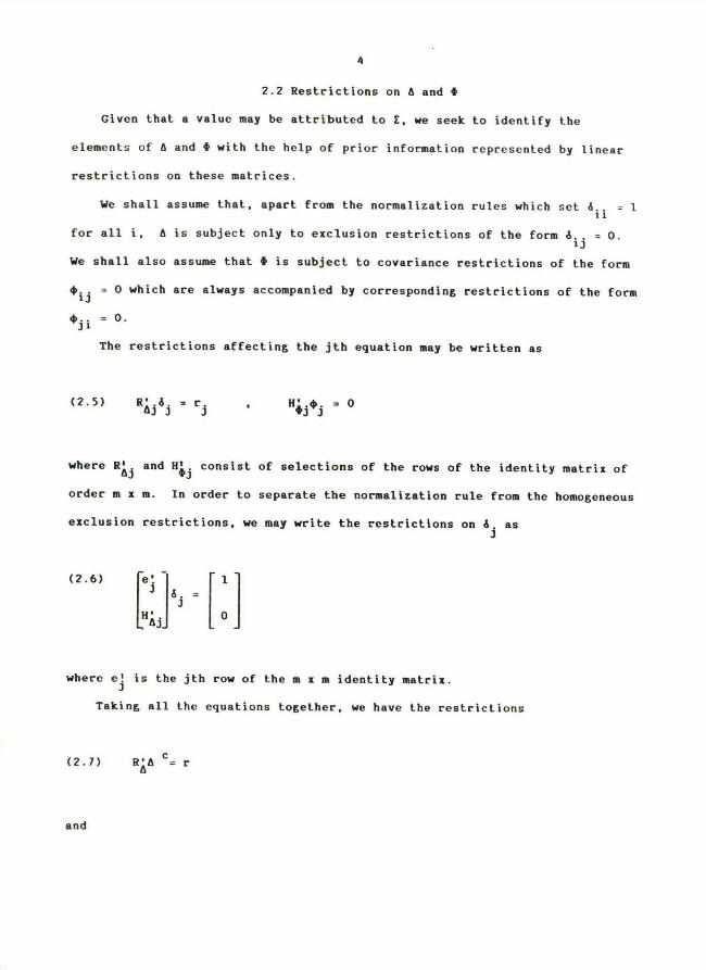
IDENTIFICATION OF LINEAR STOCHASTIC

MODELS WITH COVARIANCE RESTRICTIONS

by

Paul A. Bekker

D.S.G. Pollock

iDBNTIFICATION OF LINBAH STOCHASTIC

KODBLS MITH COVARIANCB RBSTRICTIONS

BY PAUL A. BBKKBRI AND D.S.G. POLLOCK2

The purpose of this paper is to provide a systematic treatmentof the problem of identiEication in systems of linear structural

equations where some of the disturbances are uncorrelated.

1. INTRODUCTION

Hany oE the aspects of the claesical linear simultaneous-equations model

of econometrics have been researched in great depth, yet the problem of using

restrictions on the covariances of the structural disturbances to assist in

identífying the structural parameters appears to have received relatively

little attention.

In his seminal book on the identification problem in econometrics, F.h.

Fishec [4] did go some oE the way towards presenting an overall account of the

pcoblem; but most of his results have practical applications only in the

rather specialized case oE block-recursive systems. It should also be

mentioned that the covariance problem can be accomodated within the framework

for analysing problems of identification that Wegge (12] has provided. Other

authors, including Rothenberg (8] have added to the results, and moce

recently, the problem has been considered by Hausman and Taylor [S] in

connection with limited-information estimation by instrumental variables. The

latter have shown that ezogeneity relationships induced by covaríance

restrictions may find expression in a class of models that is wider than that

pport of the1~ Paul Bekker wishes to acknowledge the financial suNetherlands Organization for the Advancement of Pure Research (ZHO).

2' Stephen Pollock wishes to express his gratitude to his hosts at theUniversity of Tilburg where he was resident from February 1983 to July 1983.

z

of the block-recursive models which, in its turn, is a generalization oE theclass oE recursive models analysed by ilold [13]

In this paper, we attempt to analyse, in a systematic menner, a wide

variety of relationships that may be induced by covariance cestrictions. Gie

begin our treatment of particular cases by deEining the class of decomposable

covariance restrictions. These are the restcictions that give rise to

relationships of exogeneity; and, therefore, at this stage, we are covering

much the same ground as Hausman and Tayloc. However, our treatment of the

problem is quite different Erom theirs.

By generalizing our definition of decomposability, we then proceed tointroduce the wider class of recursively decomposable restrictions. Animportant Einding is that. if all the covariance restrictions are recursivelydecomposable, then eny set of etructucal parameters that are idr.ntifiable areatso global.ly or uniquely identifiable.

In our Einal section, we consider covariance restrictions that are

indecomposable. Such restrictions no longer afford an assurance oE globalidentiEication. Nevertheless, in the case of one model which we analyse indetail, we are able to adduce a simple criterion for discriminating amongstthe isolated solutions of the identiEying equations.

Our attempt at providing a uniEied treatment of our topic rests on ananalysis of the structure oE the Jacobian matriz associated with the

identifying equations. However, we find that, in many practical cases, ourassesment of whether or not a structural equation is identified can be basedon relatively simple criteria that do not require us to take account of the

Jacobian matriz in its entirety. Nevectheless, there are cases where we dohave to resort to a full system-wide analysis; and we shall describe themethods of such an analysis in the following section.

3

2. A FORhAL ANAI,YSIS OF THH IDRNTIFLCATION PROBLR!!

2.1 The Model

ble shall conduct our analysis in tecros of a model compcising m stochasticequations in m observable variables and m unobservable disturbances. He canrepresent the model by writing

(2.1) z'A - v'

where z' - [zi,...,zm] is an observable row vector, v' -[vl,...,vm] is anunobservable disturbance vector with an expected value of S(v) - 0 and A-

[dl,...,dm] is a nonsingular m x m matrix whose ith columa contains the

coefficients of the ith structural equation.

The dispersion matrices of the vectors z and v are given by

(2.2) D(z) - E D(v) - ~ - [~1....,~m]

where ~ is assumed to be positive definite. It follows from (2.1) that

(2.3) A'EA - 4

whence we see that

(z.a) E - o.-l~0-1

is also positive definite.

If it is assumed that z is nocmally distributed. then all the information

that is available Erom the observations is contained in E which is globally

identified.

4

2.2 Restrictions on A and ~

Given that a value may be attributed to f, we seek to identify t.he

elements of 6 and á with the help oE prior information represented by linear

restrictions on these matrices.

Gie shall assume that, apart from the normalization rules which set d.. -iifor all i, A is subject only to exclusion restrictions of the form é.. - 0.i~We shall also assume that ~ is subject to covariance restcictions of the form

~ij - 0 which are always accompanied by corresponding restrictions of the form~j i - 0.

The restrictions affecting the jth equation may be written as

(2.5) Réjój - rj , H~j~j - 0

where Réj and H~j consist of selections of the rows of the identity matrix oforder m z m. In order to separate the normalization rule from the homogeneousezclusion restrictions, we may write the restrictions on dj as

(2.6) e; - 1~ d. -

JHsj o

where e! is the jth row of the m x m identlty matriz.JTaking all the equations together, we have the restrictions

(2.7) RéA c- r

and

S

(2.8) H{t c- 0

where Ac and 4c are long vectors formed by a vert[cal arrangement of thecolumns of A and i respectively.

In addition to the restrictions in (2.8), we must take account of the

symmetry of i. Let us therefore consider the operator Q, called the tensor

commutator, which has the effect that~iAc - A'c when A is any m: m matri:.This operator, which plays a fundamental role in the theory of matriz

diEferential calculus, has been defined by numerous authors including ealestra

[1], Magnus and Neudeckec [6] and Pollock [1]. In the present context,

.-r - Ei~(ejei ~ eie~) is a partitioned matrix of ordec m2 z m2 whose j[th

block is the matriz eie: of order m x m which has a unit in the ijthJ

position and zeros elsewhere. Using the commutator, we can express the

symmetry oE ~ by wciting the equat[ons

0

The set of all matrices [A, ~] that obey the restrict[ons under (?.7),

(2.8) and (2.9), in addition to the restrictions that A is nonsingular and

that ~ is positive definite, will be called the restricted parameter set.

The symmetcy of ~ can also be expressed by wciting the equation

~c - lI2(I i~;i,)4c . On substituting this into the equation under (2.8), we

obtain the expression

(2.10) lI2H~(I t~)fc- 0 .

These equations are symmetric in the arguments ~i~ and ~ji. It follows that

the restcíction setting ~ „i~setting ~ji to zero; and we

Given that ~c - (e'Ee)c

6

to zero is now identical to the restriction

are free to eliminate one of these.

-(I (~,e'E)ec , and that e'E -~e 1, it follows

that we can rewrite the equations in (2.10) in the form

(2.11) lI2H{(I i~)(I(ZG e'E)ec

- lI2H~(I i(~)(I ~Sy' ~e-1)ec

Thus we see that the linear restrictions on ~c give rise to a set of bilinear

ristrictions on ec .

On combining the equations from (2.1) and (2.11), we obtain the system

(2.12) R'e

172H~(I .(1,)(I Y~`e'E)

2.3 General Conditions Eor ldentifiability

L~quation (2.3) shows that, for a given value of E, the value of ~ is

uniquely determined by that of A. Therefore the problem of identification

rests with A alone.

The equations (2.12) contain all the information relating to e, and weshall describe them as the identifying equations. Any value of ec whichsatisfies these equations may be termed an admissible value. The trueparameter value e0 is clearly an admissible value, and our object is to

establish conditions under which it represents a locally isolated solution ofthe identiEying equations such that, within the set of values of e obeying thereatrictions in (2.7), there exists an open neighbourhood of e0 containing no

iother admissible value.

It is well known that a sufficient condition for A~ to be locally isolated

is that the Jacobian matri: of the transformation in (2.12) evaluated at A~

has full column rank. By differentiating the function with respect to A, we

find that the Jacobian is

(2.13) R'JE(e; E) ~

e

Há(I i(j,)(I(~A'E)I

Let á0 be the true value oE i. Then, since A'E ~ fA-1 , it follows that

the matrix function

(2.14) xé -

H{(I a t-r)(I~1~A-1)

has the same value at the point [A0, ~~I as the functíon JE(A; E) has at the

point A~ . If it can be established that J(A, 4) has full cank for almost

every point in the restricted parameter set, then the fulfillment of the

condition on the rank oE JE(A; E) at AO is virtually assured.

The condition that J(A~, ~Q) has full rank, which is sufficient for the

local isolation or identification of A~ . becomes a necessary condition as

well if it is assumed that [A0, ~O1 is a regular point of J(A, i) such that

there exists an open neighbourhood of [A~, f0] in the restricted parameter set

for which J(A, f) has constant rank. This is an acceptable assumptlon since

the set oE irregular points is of ineasure zero; which can be demonstrated by

using a result oE Fisher [3, Th. S.A.2] concerning the roots of analytic

functions. We state the following:

J(A, ~) -

8

ASSUKPTION 1: The true parameter point [AO. ~O] is a regular point of J.

In considering the identification of the parameters of a single structural

equation, we will make a further assumption:

ASSUMPTION 2: [AO, ~O] is a regular point of J! ; }. - 1,...,m where JR -

J(ei ~~ I) is the submatriz of J-[J1....,Jm] corresponding to the derivative

taken with respect to the parameters of the Rth equation.

Rothenberg [8] has used an analogous assumption in his Theorem 8 which

recapitulates on a theorem by Hald [11] which is also proved by Fisher [3].

He shall restate the theorem in the form which best suits our own purposes:

PROPOSITION 1: A necessary and sufficient conditlon Eor the parameters of the

first eguatlon to be locally isolated is that Rank(J) - Rank(J1) i

Rank(J2,...,Jm) and Rank(J1) - m .

41e can state equivalent conditlons for identification in terms of any matrix

that can be derived by postmultiplying J by a nonsingular matrix of order

m2 x m2 . On postmultiplying J by I~ A, we obtain

(2.15) FU R~(I v`~~ A)

F - -

F~ H~(I i '-~)(I~Jf)

- [Fl, . . . . Fm]

where FR - F(ei ~~I) . Clearly, we have Rank(F) - Rank(J) and Rank(Ft) -

Rank(J!). ltoreover, F and FR have the same regular points as J and JR

respectively.

9

we may note that Rank(F1) ~ m is a nesessary conditíon for the first equation

to be identified; and this corresponds to Fisher's Generalized Rank Condition

[3, Th 4.6.2].

The advantage of using F comes from the fact that it separates the

matrices ~ and e, which facilitates the assesment of its rank.

2.4 The stcucture of the Matriz F

we shall now look more closely at the structure of the matri: F.

The submatriz FD corresponding to the restrictions on e has a relatively

simple structure:

(2.16) FD - bté(I ~ e)

Re1e . 0 . . . . , 0

o , es2e , . . . , o

o , o ,...,R'e

- [F01 ,

If there were no covariance restrictions, then the equation Rank(F) -

~Rank(F~) would always hold. Howevec, the covariance restrictions tie

together the sets of identifying equations, and this is reflected in the

structure of the submatriz F~ .

To illustrate the structure of F{, imagine that its rth row fr corresponds

to the restriction ~i~ -(e~ ~ eí)ic - 0. Then

(2.11) fr - (e3~ei)(I t(~)(I~j~:4)

- (e3 ~ eif) t (ei q e~f)

~ [Ec1, . . . , frm]

10

Here we have a 1 z m2 row vector consisting oE subvectors Er! ; i- 1,...,m of

order 1: m. These are zeros apart from the ith subvector f' -~j and therijth subvector f~j - ~i .

For a complete ezample, let us consider the case of the model specified by

the matrices:

(2.18) 1 ,d12, 0A - 0 , 1 ,d23

d31, 0 , 1

~11' 0 , 0-. i - 0 ,~22, 0

0 ' 0 '~33

The matriz F is then given by

(2.19)

IF1,F2,F3] -

1 'd12' 0 : :0 , 1 ,d23: :...................................

: 0 . 1 .d23::d31' 0 ' 1 :...................................: : 1 'd12' 0

: :d31' 0 , 1

dll - 1d21 - 0

d22 - 1d32 s 0

d13 - 0d33 - 1

~12 - 0m13 - 0~23 - 0

0,m22, 0:~11, 0, 0: 0, 0, 0

0' 0'~33: 0' 0' 0:~11' 0, 0

0' 0' 0: 0' 0'~33: 0.~22. 0

Here the empty blocks signify submatrices containing only zecos. The rows of

F correspond to the restrictions written in the margin.

The rows of F corresponding to the normalization rules dll, d22, d33 - 1are linearly independent of all other rows; for each contains a unit which

falls in a column where all the other elements are zeros. By deleting theserows and the cocresponding columns, we obtain a submatriz which has fullcolumn rank if and only if F has full column rank. By permutating the rows oF

il

xthe submatriz in question, we obtain the matriz F which appears in the

following equation (2.20):

(2.20) FaFx9 - 1x q

r~22' 0'~11' 0' 0' 0-0 ,~33, 0 , 0 ,dll, 0

1,d23, 0, 0, 0, 0

0, 0,d31, 1, 0, 00 ' 0 ' 0 '~33' 0 '~220, 0, 0, 0, 1,d12.......................

r ~11

~11d31d12

~011(1-d23d31d12~

It is evident that the rows of the matriz Fxl , which is in echelon form,

are linearly independent. If d23d31d12 ~ 1, then the vectoc q, which isx x xorthogonal to the rows oE F1 , is not orthogonal to E2 . Therefoce, f2 cannot

xbe a linear combination of the rows of F1 and, consequently, Fx and F are offull rank. It follows that the parameters are locally identified. If

d23d31d12 - 1, then the parameter point is irregular and is thereEore

excluded from our analysis. However, the irregular points constítute a set oE

measure zero.

3. DECOHPOSABILITY

A covariance term within the dispersion matrix f- A'EA is a bilineac

function of the parameter vectors of two structural equations. Therefore onemight ezpect a covariance restriction to have the eEfect, always, of tying

togethec the identification problems of two equations. However, it often

f2

12

happens, as a result of a particular conjunction of the restrictions on A and~, that a set of covariance restrictions becomes a set of linear cestrictions

on the parameters oE the jth equation which makes no reference to the values

of other stcuctural parameters. In sucó cases, we shall say that we have a

set of decomposable restrictlons.

Nhen all the available covariance restrictions are decomposable, the

problems of identifying individual equations are separable, and, if the

parametecs of an equation are identiEiable, then they are uniquely or globallyidentifiable.

In our chacacterization of decomposable covariance restrictions, we shallmake use of the following lemma in which the notation makes allusions to

section 2.á.

L6lQiA 1: Consider the matrix

(3.1) FO FQi ~ FO -

F- f. - f. ~ f.3 - C Fi ~ FJ J1 li lj

wherein fii, fi~ are row vectors and Rank(FD) - Rank(FDi) i Rank(F0~) . Then

Rank(F) - Rank(Fi) t Rank(F3) iE and only iE fii is linearly dependent on therows of F~i or fi3 is linearly dependent on the rows oE F~J

The proof of this appears i n the appendi:.

3.1 Decomposable Covariance Restrictions

ile may begin our account with the definition of a decomposable covariancerestciction.

13

D6F1NIT10N 1: 41e say that the restriction ~ij - 0 i s decomposable if, for all

points in the restricted parameter set, we have

(3.2) FOi ' FO - FOi - FORank j - Rank t Rank j

where FOi and FOj are defined in (2.16).

L6t~4(A 2: The restriction ~i3 - 0 is decomposable if and only if (a) for ell

points in the restricted parameter set, there exists a vector ~i such that ~3

- A'Róí~i or (b) for all points in the restricted pacameter set, there exists

a vector kj such that ~i - A'Rejkj.

The proof follows immediately from Lemma 1. If conditions (a) and (b) are

fulfilled at the the same time, then the restriction ~ij - 0 is of no

assistance in identlEying the equations, and we say that it is redundant. If

condition (a) holds together with the condition that Rank(A'Re3, ~i) -

Rank(A'Re ) a 1 for all regular points of [A'Rej, ~i], then the restriction isj

said to be assignable to the jth equation, and we call the ith equation the

instrumental equation.

To illustrate the definition and the lemma, we may consider the model

specified by the matrices

(3.3) 1 , 0 ,d13, 0 ~11'~12'~13' 00 , 1 , 0 ,d24 ~21'~22'~23'~24

ó - d31, 0 , 1 .é34 ' ~ - ~31.~32.m33. 00,d42, 0, 1 0.m42' 0'~44

The restriction ~14 - 0 is decomposable. This can be seen by considering

~~ . ~i ~~ ~i

the matri:

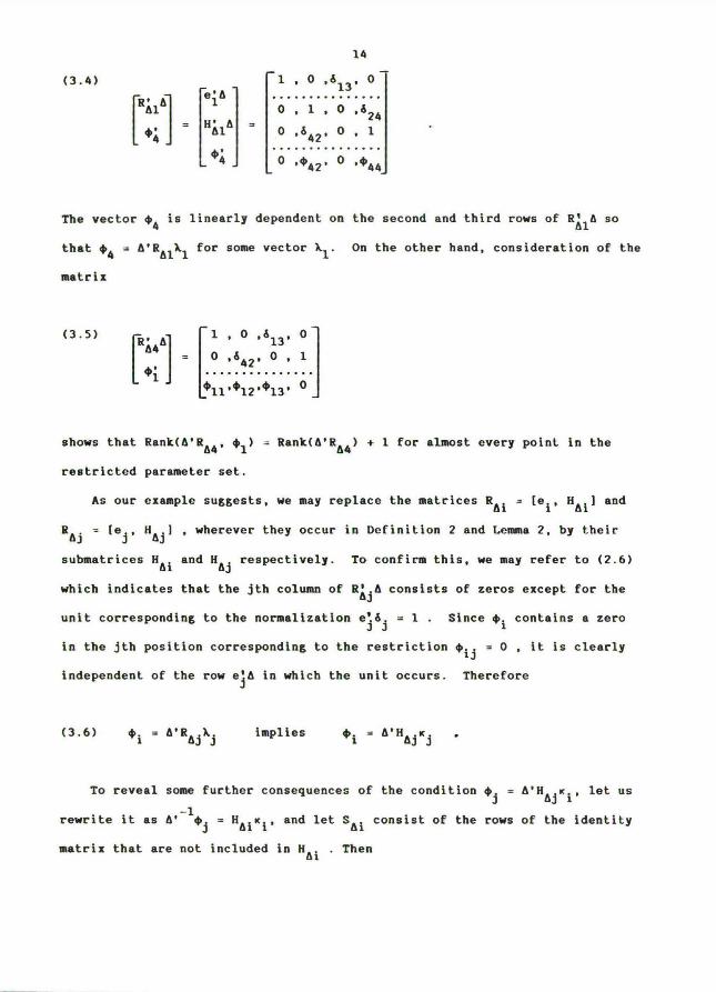
(3.á)

141 , 0 ,d13, 0

, e'eRe1e 1 0' 1' o'd2a~4 - Héle - o .d42' o , 1

, ........... ..~4 .0 '~42' D '~44

The vector ~4 is linearly dependent on the second and third rows of Rsle so

that ~4 - e~Rel~l for some vector ~1. On the other hand, consideration oE the

matrix

(3.5) R. e 1. ~.d13. 0e4 - 0 ,d42, 0 , 1~1 ..............

~11'~12'~13' D,

shows that Rank(e'Re4, ~1) - Rank(e'Rea) t 1 for almost every point in the

restricted parameter set.

As our example suggests, we may replace the matrices Rei -[ei, Hei] and

Re~ -[e~, He~] , wherever they occur in Definit[on 2 and Lemma 2, by their

submatrices He1 and He~ respect[vely. To confirm this, we may refer to (2.6)

which indicates that the jth column of Ré3e consists of zeros except for the

unit corresponding to the normalization e~d~ - 1. Since ~i contains a zero

in the jth position corresponding to the restriction ~i3 - 0, it is clearly

independent of the row e3e in which the unit occurs. Therefore

(3.6) ~i - e'Re3~j i mplies ~i - e'He3K~ .

To reveal some further consequences of the condition m3 - e'He~Ki, let us

rewrite it as e'-1~~ - HeiKi, and let Sei cons[st of the rows of the identity

matrix that are not included i n Hei . Then

15

(3.7)Hei -1 HeiNei Kie' ~. - Ki - :se. SeiHei o

and we can see that ~j - e'He1Ki if and only iE seie'-l~j - 0. At the true

parameter point, or at any other admissible point where e'-14 - Ee. the latter

becomes SsiYdj - o which is a set of linear restrictlons on dj. This equation

can also be written as

(3.a) séín(z)dj 3 C(Séiz. a~z)

- c(séíZ, v~) - o

which indicates that the disturbance term vj is uncorrelated with all the

variaDles entering the ith equation. we may describe this situation by saying

that the variables entering the ith equation are exogenous relative to the jth

equation; and these variables may be used as instruments for the

identification and estimation oE the jth equation.

The next proposition indicates a way of determining whether or not a

particular covariance restriction is decomposable.

PROPOSITION 2: The decomposability condition ~j - e'HeíKi, relating to the

covaciance restriction mij - 0, holds for every point in the restricted

parameter set iE and only iE there exist selection matrices N and Nq m-q.

selecting q and m-q different columns respectively, such that

(3.9) N~-qHéíeH~jNq - o

The proof appears in the appendix.

16

L~quation (3.9) shows that the restriction N~ qHéidi - 0 holds not just for

a single equation but for q equations, indexed by i- il,...,iq, whose

parameter vectors are selected from the matrix A by the matrix H~jNq. Thus

the equation i s common to a set of q decomposability conditions ~j - e~HAiKi 'i- ll,...,iq relating to a set of q covariance restrictions ~ij - 0; i-

iYe should note that g is also the number oE distinct variables entering

the equations indexed by i- il,...,iq. The g variables are not necessacily

present in each of these equations, and so the condition (3.8) may represent

less than the full set of exogeneity relationships aEEecting the jth equation.

To illustrate the condition (3.9), let us consider again the model

speciEied under (3.3). Corresponding to the restriction ~14 - 0 which

satisfies the decomposability condition ~4 - A'Rel~l, we have the equation

(3.10) -1 , 0 ,d13, 0 1 , 0

H. eH - r ó: ó: ó; 0 1 do : Ó: o:á24 Ó: o - r ó; Ó 1.el ~4 L J L 131 34

The equation He3AH~4 - 0 which corresponds to the restriction ~34 - 0 is

identical to the above. Thus the two vaciables zl and z3 entering the

equations 1 and 3 are ezogenous relative to equation 4; and both can be used

as instruments.

In order to deal with cases where there are a number oE decomposable

restrictions relating to diEferent equations and, also, to provide a basis for

dealing, in the next section, with recursively decomposable restrictions, it

is helpful to generalize Lemma 1 to obtain the following:

0,d42, 0, 1 0, 0

17

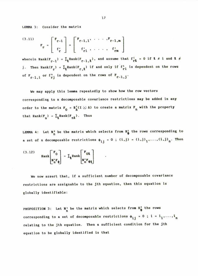
LBl4~A 3: Consider the matrix

(3.11) Fr-1 ~ ~ Fr-1,1' ' . .'Fr-l,m

Fr - fr - fcl ' ' ' ' ' frm

wherein Rank(Fr-1) - ~lRank(Fr-1,i)' and assume that fT! - 0 if ! f i and !~

j. Then Rank(Fr) - ElRank(Fr~i) if and only i f ETi is dependent on the rows

of Fr-l,i or f~j is dependent on the rows of Fr-l,j.

We may apply this lemma repeatedly to show how the cow vectors

corresponding to n decomposable covariance restrictions may be added in any

order to the matri: FO - Ré(I ~y A) to create a matri: Fn with the property

that Rank(Fn) - ElRank(Fni). Thus

L6NltA 4: Let N~ be the matrix which selects from H~ the rows corresponding to

a set of n decomposable cestrictions ~ij - 0;(i,j) -(i.j)1,...,(i,j)n. Then

(3.12)Rank O - ElRank

NnF4 NnF4A

We now assert that, if a sufficient numbec of decomposable covariance

restrictions are assignable to the jth equatlon, then this equation is

globally identifiable:

PROPOSITION 3: Let N~ be the matrix which selects from N~ the rows

corresponding to a set of decomposable restrictions ~ij - 0; i- il,....in

relating to the jth equation. Then a sufficient condition for the jth

equation to be globally identified is that

F FO!

18

(3.13) FDRank ~ - m .

NnF~j

IE every covariance restriction which references the jth equation belongs to

this set of n decomposable restrictions, then this condition is necessary as

well.

Here local identification follows Erom Proposition 1 and Lemma 4. Global

identiEication follows Erom the fact that decomposable covariance restrictions

give rise to linear restrictions on A.

We can also represent the condition (3.13) by writing

(3.14) RéjeRank - m

NóH~j~

where An is the appropriate selection matrix operating on H~ .j

To illustrate this condition, we return again to our example under (3.3).

Ye see that a necessary and sufficient condition for the fourth equation to be

identified is that the matrix

(3.15) 1 , 0 ,d13, 0

Ré40 0 ,d42, 0 , 1

.H~4~ ~11,~12,~13, 0

~31'm32'~33' G

is nonsingular. The condition will be satisfied by every regular point in the

restricted parameter set; and, according to Assumption 2, these are the only

points we need consider.

19

4. RECURSIVE DECOM[POSARILITY

i~ie begin with a general deEinition of recursively decomposable restrictions

DEFINITION 2: Let mij - 0 ;(i,j) -(i,j)1,...,(i,j)n be a set of covariance

restrictions corresponding to the rows fi,...,f~ of the matriz F~ , and let us

define, for r- 1,...,n , the matrices

(4.1) Fr-1 Fr-1,1, . . . ~Fr-l,mF - -r , ,fr f~l , . . . , E~

with FO - Ré(I~~{~A). Then, if, at every regular point oE Fr-.1 within the

restricted parameter set, we have

(4.2) Rank(Fr) - ~lRank(Fr,!)

for all r, we say that the covariance restrictions are recursivelydecomposable.

It is clear that the first in a sequence of recursively decomposable

restcictions must be a decomposable restciction according to Definition 2.

lioreover all decomposable restrictions are also recursively decomposable.

T,P.l4lA 6: If the first r- 1 restrictions are recursively decomposable, then

the cth restriction ~ij - 0 is recursively decomposable if and only if (a) for

ell regular points of Fr-1, there ezists a vector kí such that ~j - Fr-l,ikior (b) for all regular points oE Fr-1, there exists a vector kj such that ~i -

iFr-1, j~j ~

The proof of this follows directly from Lemsa 3. IE the condition (a)

20

holds together with the condition that Rank(Fr'~) - Rank(Fr-1~~) i 1 for all

regular points of Fr~~ , then the restriction is said to be assignable to the

jth equation, and the ith equation is said to be the instrumental equation.

For an example, let us consider the model specified by the matcices

(4.3) 1, 0.a13' ~ ~11' ~'~13' ~-o. 1. 0.ó24 0.~22.~23, 0

ó - d31, 0 , 1 .ó34 ' ~ ~ ~31.~32.~33, 00,ó42, 0, 1 0, 0. 0 ~~44

which may be obtained from the model specified in (3.3) by setting ~42, ~21 -0. The corresponding matrix F is givea by

(4.4) RélA, 0 , 0 , 0

o ,Re2e, o , oo , o ,RS3e, o

I Fo I - .o....0....0...~e4s~á . o . o . ~i

.

o . o . ~á . m3

o . ~4 , o . ~2

~2 . ~i . ~ . 0

.1 : ~14 - 0.2 ~ ~34 -.3 : ~42 - 0.4 ' ~21 ~

~le already know, from the analysis oE section 3, that the cestrictions

~14' ~34 " 0 are decomposable; and in the present example, they represent the

first two restrictions in a recursively decomposable sequence. The

restriction ~42 - 0 is the third in the sequence; for consideration oE the

matri:

21(4.5) - 1 , 0 ,d13, 0

0 ,d42. 0 , 1~11, 0 .~13. 0

~31'~32'~33' 00 ,~22,~23, 0

shows that ~2 - F2,4)`4 for all regular points of F2~4 and of F2.

Finally, the restriction ~21 - 0 i s also recursively decomposable; Eoc

consideration of the matriz

(4.6) 1 , 0 ,d13, 0-

~S2d 0 ' 1 ' D 'd24m4 ~ d31. ~ . 1 'd34

~1 D ' D ' 0 '~44LOll' D '~13' 0 J

shows that ~1 - F3,2)`2 for all regular points of F3~2 and F3.

It is easy to see that, as was the case with decomposable restrictions, we

can rewrite Definition 3 and Lemma 6 in tecros of the matriz FÓ - Hé(I ~ A)

which omits the cows of F~ cocresponding to the normalization rules. In place

of the matrices F and F of Lemtna 6, we then have Fa and Fxr-l,i r-l,j r-l,i r-l.j~

Let us also note that. for the true parameter point, or for any other

admissible point, we can write F~-1,! - Jr-1,le where Jr-1~! ia a submatriz of

JE(A, ~) from which the row corresponding to the normalization rule has been

deleted. At such points, the decomposability condition (a) in Lemma 6 can be

written in the form

(4.1) Ed~ - J~~1,iKi

In section 3.1, we showed that each decomposable covariance restriction

corresponds to a set of linear restrictions on structural parameters. Ye

22

shall now show, more generally, that each recursively decomposable restciction

corresponds to a set oE linear restrictlons.

Let us therefore consider a Eull system of restrictions where the first pcovariance restrictions form a recursively decomposable sequence. Then wehave the following conditions:

(4.8) Héldi - 0 ; ! - 1,...,m

di Edj - 0 ; r- 1,...,nr r

Edj - J~'l~i K i ; r- 1,....Pr r r

We can demonstrate that these are equivalent to the conditions

(4.9) Héld! - 0 ; i - 1,...,m

Br.j Edj - 0 ; r- 1,....Pr r

di Ed. - 0 ; r- ptl,...,n ,r ~r

wherein the matrices Br~j depend only on E.r

The matrices Br~j may be defined recursively. When r - 1, B1' is ar ~1

matri: of Linearly independent columns that are orthogonal and complementary to

those of Hei such that B1~ Hei - 0 whilst [Hei , B1 ] is nonsingular. In1 jl 1 1 '~1

addition, we define a set of matrices BI~R ;!- 1,...,m of the same order as

Bl~j but consisting of zeros when !~ j. For other values of r not exceeding1

p, we define er~j to be a matrix whose columns are orthogonal and complementaryr

to those of the matriz

[Hei , E(Bl~i , B2~i ,....Br-l,i )1:r r r r

and we also define the matrices er~! - 0 for R~ jr which are oE the same order.

23

We use the principle of induction to demonstcate the equivalence oE (4.8)

and (4.9). Let r- 1. Then the restriction d: Eé. - 0 is decomposable such11 J1

that Ed. - H K. and, consequently, B' Ed. - 0. Conversely, as dJ1 Ail tl l.jl J1 i1is a vector in the null space of Héi , and as B1~ forms a basis of that space.

1 J1it follows that di - 81 ul for some N1; and, therefore, the conditlon

1 'J1Bi~j Edj - 0 implies the condition dí Eój - 0. Since Hei focros a basis

1 1 1 1 1oE the null space oE Bi~j , the condition Bi~j Eój - 0 also implies that Edj

1 1 1 1- HAi Ki for some Ki , which is the decomposability condition. Thus the first

1 1 1covariance restriction and its associated decomposability condition are equivalent

to the linear restrictions Bi~j Edj - 0 and may be replaced by the latter.1 1

Now assume that the replacement is valid for the first r- 1 recursivelydecomposable restrictions. Then, for the rth restriction, the decomposability

condition Eój - Jr'l~i K i may be written asr r r

Eójr - IHAir, E(B1~iry1,....Br-l,irpr-1)iKir

so that B~.j Edj - 0. Conversely, since ói - Br~j Nr Eor some yr, it followsr r r r

thet the linear restrictions Br~j Edj - 0 imply ói Edj - 0 together withr r r r

its associated decomposability condition. Thus the rth covariance restriction

may be replaced by a set oE linear restrictions.

Our argument has served to demonstrate the following:

PROPOSITION 4: If the first p covariance restrictlons are recursively

decomposable, then a sufficient condition for the jth equation to be globally

identifiable is that

(4.9) Rank(Fp~j) - m

If all the covariance restrictions which reference the jth equation are in

this set of p restrictions, then the condition is necessary as well.

2aS. THE CI,ASSICAL NODKL

The classical simultaneous-equations system of econometrics is a special

case of our model which can be written in the fono of (2.1) as a

block-recursive system:

(5.1) rI' , 0[Y'. z'1I - [c'. E'1

LB . A

The vector z contains Ic vaciables that are exogenous relative to the G jointly

dependent variables in y. The dispersion matrices for z' -(y', z'] and v' -[c', ~'] take the forms of

(5.2) E- EYY~ EYz ~- I~' 0 1Ezy. Ezz . L 0 . A J

The nondiagonal blocks of ~ are set to zero by the covariance restrictions

~ij, ~ji - 0 where j- 1,...,G and i- Gf1,...,GtR. These restrictions ace

all decomposable as can be seen by considering

(5.3) HéiA !' , 0

m~ ~Y~ , 0

where Hé1 is the matriz associated with the restrictions dli "" 'óGi - 0relating to any column of the zero matriz i n (S.1). Since fis nonsingular,(5.3) shows that ~j -[~~, 0] is dependent on the rows of HéíA - [1', 0] . Infact, the zero block of (I', 0] cocresponds to the matri: selected in (3.9).

25

In treating the identification problem of the classical system, we shall

confine our attention to cases where the restrictions on ~ are recucsively

decomposable. The identiEication of the jth equation, where j~ G, may then

be assessed by considering the matrix consisting of the nonzero row vectors oE

Fj

(5.4)R~,j, 0 r C . 0 l

R' C 0L JII rj ~RéjA 0,Háj B. A H' B, H' ABj B3H~j} - .H~~;.Ó....~.;.~. N.;~:..ó..

C lC ~ :A necessary and sufficient conditon for the identifiability of the jth

equation is that this matrix has a rank of m- G i K. However, since the K x K

matrix 6 - A'ExxA is nonsingular, thie is equivalent to the condition that

(5.5) R'.Cf~

Rank HBjB - G .

In the absence of restrictions on ~, the term H~jY in (5.5) is

suppressed, and we obtain the conventional rank condition which is stated by

Schmidt í9, p.134] amongst others.

As a corollary to Lemma 6, we have the following statement which is

analogous to Lemma 2:

H,~,j!'

0, I- 0, A 0 , 9

26

COROLLARY 1: In the classical simultaneous-equations system, the restrictions

on T are recursively decomposable only if there exists a covariance

restriction ~i~ - 0 such that (a) at

we have ~~ -[T'RTi' B'HBi]ki for some

every regular point of [C'RTi, B'HBi],vector k.i or (b) at every

of [C'Rr~, B'HB~], we have ~i -[T'Rr~, B'HB~]k~ for some k~.

regular point

Of course, we can replace the matrices Rri -[ei' Hfi] and RT~ -[e~, Hr~]

wherever they occur in this statement by their submatrices HTí and Hr3

respectively.

We should note that, if ~i or ~~ are linear combinations oE the rows of Talone, then the covariance restriction ~i~ - 0 is, in fact, decomposable; andwe are back in the world of section 3. This cocresponds to the context inwhich Hausman and Taylor [S] have derived their propositions; for they haveconfined their attention to cases where the covariance restrictions on Y areconjoined only with restrictions on f(which they denote by B).

The following is analogous to Proposition 2~

PROPOSITION 6. The condition ~~ -[T'Hri, B'HBi]Ki relating to the

recursively decomposable restriction ~i3 - 0 holds for all regular points of

[T'H~i, B'HBi] in the restricted parameter set iE and only if there exist

selectlon matrices N and N such thatq G-q

(5.6) N~if ~NG-9 H~3Nq - O and Rank NG- Hrir - G- q.BiB Hg;6~

The proof, which i s analogous to that oF Proposition 2, is given in theappendi:

For an example, let us considec the model specified by the matrices

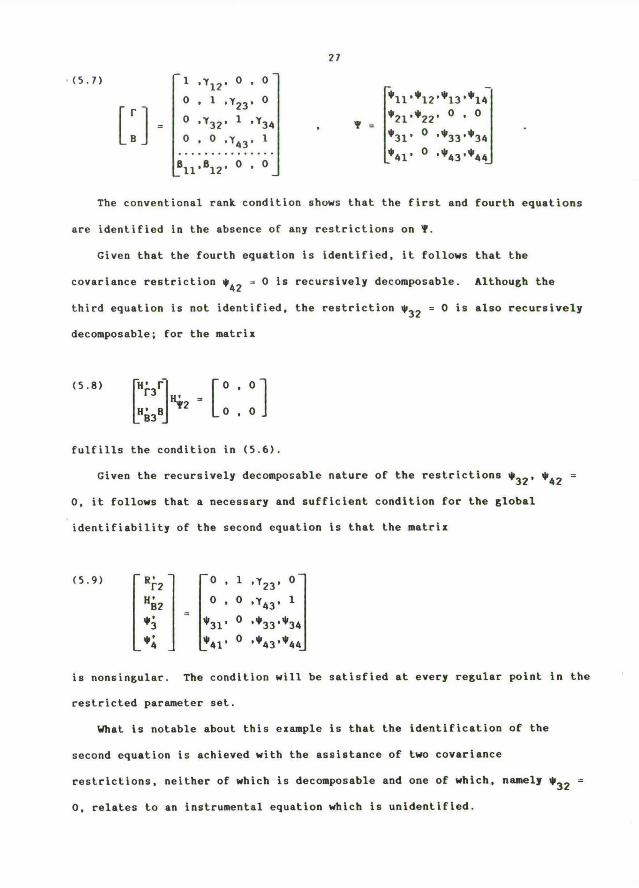
27

[,11 ,Y12, 0 , 0

0 . 1 ,Y23, 0

0 'Y32' 1 'Y340 , 0 ,Y43, 1

Bll~~i2~.~.~.~.

ill'i12'i13'i14i21.i22. 0 , 0

~ -i31' 0 'i33'i34

i41' ~ 'i43'i44

The conventional rank condition shows that the fírst and fourth equetions

are identified in the absence of any restrictions on `[.

Given that the fourth equatíon is identified, it follows that the

covaciance restriction i42 - 0 is recursively decomposable. Although the

third equation is not identified, the restriction i32 - 0 is also recursively

decomposable; for the matrix

(s.8) Hf3f' - r 0. 0 l

HB3g 72 L o, o Jfulfills the condition in (s.6).

Given the recursively decomposable nature of the restrictions i32' i42 -0, it follows that a necessary and sufficient condition for the global

identiEiability oE the second equation is that the matrix

(5.9)

is nonsingular. The condition will be satisfied at every regular point in the

restricted parameter set.

4fi at is notable about this example is that the identification of the

second equation is achieved with the assistance of two covariance

restrictions, neither of which is decomposable and one of which, namely i32 -0, relates to an instrumental equation which is unidentified.

0 , 1 ,Y23, 0HB2 0 . ~ .T43. 1

i3 - i31' G 'i33'i34.

i4 i41' ~ 'i43'i44

28

6. INDECONPOSABLE RESTRICTiONS

We define an indecomposable covariance restriction to be any covariance

restriction that cannot be subsumed under Definition 2 of recursively

decomposable restrictions.

The effectiveness of an indecomposable restciction in assisting the

identification of a particular equation depends crucially on the way in which

other indecomposable restrictions are distributed throughout the system. In

the appendix, we prove

PROPOSITION 7: An indecomposable covariance restriction can be of assistance

in identifying equations which it references only if it belongs to a set oE s

indecomposable restrictions which reference no more than s equations.( ~ij - 0

is said to reference the ith and jth equations).

As a corollary to the proposition we have

COROLLARY 2: In a classical system with exogenous variables where all the

restrictions on Y reference the jth equation that is, where the restricttons

are confined to the jth row and column of Y- the restcictlon ~ij - 0 can be

useful for identiEication if and only if it is recursively decomposable.

6.1 An Indecomposable System

The simplest case of an indecomposable system which is locally identified

is provided by the model in section 2.4 which is specified by the matrices

29

(6.1)e- o,l,a2 1 ~11' 0 , 0 -

~ - 0 ,m22, 0

0 ' 0 '~33

We may recall that ~- A'Ee , whilst E- ioi~j has a fixed value. By

analysing the associated F inatrix, we have established that the identiEying

equations yield isolated solutions; but this does not exclude the possibility

of multiple solutions.

Consider, for example, the matrix

(6.2) 171 , -11 , 16E - -11 , 1 , -1

16 , -1 , 2

Two isolated solutions for e and ~ are given by

(6.3)

(6.4)

1 , 2 , 027

e(1) - 0 , 1 , -1

1 , 3 , 038e(2) - o , 1 , -2

160 , 0 , 10

In order to analyse the model further, we may consider the equations

(6.S) E-1 - e~- le.

1 ,ó12, 0-

-9 , 0 , 1

-19 , 0 , 12

~(1) - 0 . 25 , 0

45 , 0 , 0

95 . 0 . 02

~(2) - 0 , 25 , 0

810 , 0 , S

From these, we may derive the expression

30

(6.6) -1 -1(E )31 - d31~11

For any two solutions. we must have

(6.1) (d31~11)(1) - (d31~11)(2)

We also have d1Ed1 -~11 ~ or

(6.8) all } 2a31d31 i a33d31 - mll

Together, (6.7) and (6.8) yield

(6.9) o (d(2) - d(1)) - d(1)d(2)a ( d(2) - d(1))11 31 31 31 31 33 31 31

Therefore, if d31) ~ d312)~ we have

(6.10) d(1)d(2) - all ,31 31 e33 ~

from which it follows that there can be no more than two solutions. Analogous

expcessions hold for the other parameters; and thus we find that

(6.11) (d31d12d23)(1)- 1 (2)

(d31d12d23)

In interpreting this result. we may recall the opinion that has been

stated by F.M. Fisher [4] and, more recently. by Bentler and Freeman [2] that

simultaneous-equations models should be regarded as limiting approximations to

dynamic non-simultaneous models in which certain time lags approach zero. The

requirement that the non-simultaneous model should be dynamically stable leads

to restrictions on the matrix of parameters associated with the endogenous

variables. In particular, it is required of the classical model in (S.1) that

31

the matrix (I-f) should be convergent in the sense that

(6.12) (1-f)n ~ 0 as n

A necessary and sufficient conditioo for (6.12) to hold is that the absolute

value of the largest latent root of (I-f) is less than one. In the present

case, we have

(6.13)d31a12d23 ' 0 , 0

(I-A)3 - - 0 ' d31a12d23 ' 0

~ ' 0 ' d31d12d23

and thus, for the system in (6.1) to be stable, we require that

(6.14) ~d31a12a23~ ~ 1

This result is readily intelligible since it concerns the product oE the

coefficients that describe a circular path linking the vaciables of our model.

According to (6.11), the condition (6.14) can only hold foc one of the two

solutions of the identifying equations; and, in this sense, the model is

globally identified. In our numerical ezample, it is the solution under (6.3)

that satisfies the criterion of stability.

It is an attractive speculation to suppose that similar critecia of

stability may be available for discriminating amongst the solutions of the

identifying equations of other moce complicated models that give rise to

indecomposable problems of identification.

32

APPENDIX

LEM9A 1: Consider the matrix

(i) FO FOi ' FOJ rF - - - L F1 ~ F3 ~

fl fli ' flj

wherein fii, fi~ are row vectocs and Rank(FO) - Rank(FOi) f Rank(F0~). Then

we have

(ii) Rank(F) - Rank(Fi) t Rank(F~)

if and only iE fii is lineacly dependent on the rows of FOi or fi~ is linearly

dependent on the rows of F0~ .

PROOF: (Necessity). Imagine that, contrary to the condition, fii and fi3

are linearly independent of the rows of FOi and F0~ respectively. Then we

have Rank(F) - Rank(FO) f 1, Rank(Fi) - Rank(FOi) t 1 and Rank(F3) - Rank(F0~)

t~1 ; and so the equality under (ii) cannot hold.

(Sufficiency). Now imagine that Eii is linearly dependent on the rows of

of FOi such that fli - p.FOi for some vector p. For there to be linear

dependence between the columns of Fi and the columns of F~ , there must exist

vectors b, c such that

FOib F03c 0- ~ ~

fiib fl~c - 0

But, by assumption, we must have FOib - FO~c - 0 and, therefore, we must also

have p'FOib - flib - fl~c - 0. Therefore there exist no vectors b, c

satisfying the requirements; and so the columns oE Fi and F~ are mutually

independent. Hence the equality under (ii) must hold. I~ie may repeat

this analysis after i nterchanging F0~ and fl~ with FOi and fii respectively.

33

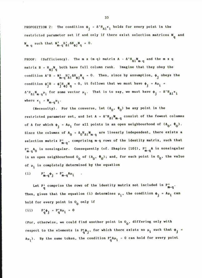
PROPOSITION 2: The condition ~~ - A'HAiKi holds for every point io the

restricted parameter set iE and only iE there ezist selection matrices Nq and

Nm such that Nm HéíAH N- 0.9 9 ~J 9

PROOF: (Sufficiency). The m:(m-q) matriz A- A'HeíNm q and the m z g

matri: B- H~~Nq both have full column rank. Imagine that they obey the

condition A'B - N~-qHéiAH~~Nq - 0. Then, since by assumption. ~~ obeys the

condition ~~B -~3N~jNq - 0, it follows that we must have ~~ - Aui -

A'He1Nm qyi for some vector yi. That is to say, we must have ~~ - A'HAíKí

where Ki - Nm quí.

(Necessity). For the converse, let (A0, 40) be any point in the

restricted parameter set, and let A- A'HeíNm q consist of the fewest columns

oE A for which m~ - Ayi for all points in an open neighbourhood of (DO' á0)'

Since the columns oF AO - AOH~iNm q are linearly independent, there ezists a

selection matri: P~-q, comprising m-q rows of the identity matriz, such that

Pm qA0 is nonsingular. Consequently (cE. Shapiro [10]), Pm-qA is nonsingular

in an open neighbourhood 00 of (A0, ~0); and, for each point in 00, the value

of yí is completely determined by the equation

(i) Pm-9~.~ - Pm-qAVi.

Let P9 comprise the rows of the identity matriz not included in P'm-q'Then, given that the equation ( i) determines pi. the condition m3 - Aui can

hold for evecy point in 00 only if

(ii) P9~~ - PQAVi - 0

(For, otherwise, we could find another point in 00, differing only with

respect to the elements in P9~~, for which there ezists no Ni such that ~j -

Aui). By the same token, the condition P9Ayi - 0 can hold for every point

34

only if P'A - 0 identically (For, otherwise, we could always Eind a point in9

00 generating a nonzero column corresponding to a nonzero element of Ni).

Finally, since H~~~3 - 0 comprises all the zero restrictions on ~~, we

must have Pq - N9H~~; and so the condition PqA - 0 is the condition that

N~H~.A'H M - 0.q~~ A i m- q

PROPOSITION 6: The condition dr3 - IC'HCi' B'HBí]K; relating to the

recursively decomposable restriction ~i~ - 0 holds Eor all regular points of

[i" HCi, B'HBi] in the restricted parameter set iE and only iE there exist

selection matrices Nq and N~ q such that

. .NG HCíC H,r3Nq - 0 and Rank NG-q HC1 - G- q

q HBiB HBiB

PROOF: (Sufficiency). The proof is analogous to that of Proposition 2.

(Necessity). Let (A0, f0) be any regular point of [C'HCi, B'HBi] within

the restricted parameter set, and let A-[C'HCi, B'HBí]N~ q consist of the

Eewest columns for which ~y3 - ANi holds in an open neighbourhood of (SO' ~0)

in which A has constant rank. Then, at the point (A0, ~O), the matrix A- AO

must have full column cank. For let us write A-[al, A2] and let us assume,

to the contrary, that al is dependent on A2. Then, in each neighbourhood oE

(AO, f0), we could find a point (Ax, 4x) for which al is independent oE A2 -

for othecwise the matriz A would not consist of the fewest columns. But this

would imply that

Rank(AZ)0 - Rank(A)0 - Rank(A)a - Rank(A2)a ~ 1

or simply Rank(AZ)O ~ Rank(A2)y~, which cannot be true since, by virtue of the

semicontinuity of rank (cf. Shapiro [10]), a matriz sufficiently close to (A2)O

must have Rank(A2),~ 3 Rank(A2)0. Thus it is established that A has full

column rank at (A0, ~0); and the proof may now proceed along the lines of the

prooE of Proposition 2.

35

PKOPOSITION 7: An indecomposable covariance restrictlon can be of assístance

in identifying equations only iE it belongs to a set oE s indecomposable

restrictions which reference no more that s equations. (~ij - 0 is said to

reference the ith and j th equations).

PROOF: imagine that, for every subset oE the indecomposable restrictions, the

number t of equations that are referenced is greater than the number s of

restrictions. Select any restriction ~pq - 0, and let the pth and qth

equations be the first and second in a renumbered sequence of equations

indexed by j- 1,...,t. We can construct this sequence in euch a way that, if

all the restrictions ace written in the form ~ij - 0 with i G j, then there is

no more than one such restriction for every j.

Now consider the matrix

P - -

Fr Frl' . . . 'Frt'Fr,ttl' . . . 'F~

Fs Fsl, . . . ,Fst, 0 , . . . , 0

- C Fl , . . . . Ft'Fttl ~ . . . . Fm ~

where Fr comprises FO - Re(I GS'A) and the rows corresponding to r recursívely

decomposable restrictions, whilst Fs is a matriz in lower echelon form

comprising the rows corresponding to the indecomposable restrictions ~ij - 0;

i G j ordered according the index j. Then, for j- 1,...,t ,we can find

vectors aj such Frjkj - 0 whilst Fsjkj ~ 0. The matrix [Fs2k2,...,FstAt) is

in lower echelon form and is, consequently, of full row rank. Nence there

exists a vector N such that Fs1A1 -[Fs2'' "'Fst)p whilst Frl)`1 -

(FrZ,...,Frt]p - 0; and, therefore, the condition Rank(F) - Rank(F1) t

Rank(F2,...,Fm), which is necessary for the identificetion oE the first

equation, cannot hold.

36

REFBRENCES

[1] BALESTRA, P.: La Derivation Katricielle. Paris: Sirey, 1976.

[2] BBNTLBR, P. M. and 6. H. FRBBltAN: "Tests for Stability in LinearStructural Bquation Systems," Psychometrica, 48(1983), 143-145.

[3] FISHBR, F. M.: The IdentiEication Problem in Bconometrics. New York:McGraw-Hill, 1966.

[4] FISHER, F. M.: "A Correspondence Principle for Simultaneous Kodels,"Bconometcica, 38(1970), 73-145.

[S] HAUSNAN, J. A. and Y. 6. TAYLOR: "Identification in Linear SimultaneousBquations Kodels with Covariance Restrictions: An Instrumental VariablesInterpretation," Bconometrica S1(1983), 1527-1549.

(6] MAGNUS, J. R. and H. NBUDECKER: "The Commutation Matrix: Some Propertiesand Applications," Annals of Kathematical Statistics, 1(1979), 381-394.

[7] POLLOCK, D. S. G.: The Algebra oE Econometrics. Chichester: John Wileyand Sons, 1919.

[8] ROTHENBERG, T. J.: "IdentiEication i n Parametric Models," Bconometrica,39(1971), 577-579.

[91 SCHMIUT, P.: Bconometrics. New York: Karcel Dekker, 1916.

[10] SHAPIRO, A.: "On Local Identifiability in the Analysis of MomentStructures," unpublished paper. The Department of Kathematics of theUniversity of South AErica.

[11J WALD, A.: "Note on the Identification of óconomic Relations," inStatistical Inference in Dynamic Economic Kodels. New York: John Wileyand Sons, 1950.

(12] WBGGB, L.: "Identifiability Criteria for a System of Equations as aWhole," The Australian Journal of Statistics, 1(1965), 67-77.

(13] {aOLD, H., in association with L. Jureen: Demand Analysis: A Study inBconometrics. New York: John Wiley and Sons, 1953.

N I~ I ~NNBIÍ~YIV ~I ~Í~1 VÍw~WI~ I V