76261984156

Bestemming

~~U

TIjJSCNRIFTENBUREAUBIBLIC}TL3~.~- ci;KATi::~LiLY~HOGï:SCi-iJOL

TILBURG

subfaculteit der econometrie

RESEARCH MEMORANDUM

Nr.

I~~INIIIIIIIIIIII IIIIIIII IIIII~III II~'Jllllql

TILBURG UNIVERSITY

DEPARTMENT OF ECONOMICSPostbus 90153 - 5000 LE TilburgNetherlands

FEW

156

AN INPUT-OUTPUT LIKE CORPORATE MODELINCLUDING MULTIPLE TECHNOLOGIES ANDMAKE-OR-BUY DECISIONS

Bert R. Meijboom

October 1984

Contents

Abstract

1. Introduction

2. Problem formulation

2.1. The firm in input-output terms

2.2. Central Problem

2.3. A decision model

3. Formalization

3.1. Indices

3.2. Names

3.3. Internal structure

3.4. Conventions for vector inequalities

4. Development of the decision model: the sectors 'End products' and

'Intermediate products' with multiple technologies

4.1. Introduction

4.2. Primary input; final output

4.3. Technology

4.4. Linear programming formulation of the decision model

4.5. Properties of the LP model

5. The incorporation of technical services5.1. Introduction5.2. Make-or-buy decisions5.3. The case with a constant demand for technical services5.4. The case where the demand for technical services depends on the

product divisions

6. Summary

References

Figures

i

AN INPUT-OUTPUT LIKE CORPORATE MODEL INCLUDING MULTIPLE TECHNOLOGIES AND

MAKE-OR-BUY DECISIONS

B.R. Meijbooml)

Subfaculty of Econometrics, Tilburg University, The Netherlands

A substantial part of our research project "The analysis of multileveldecisions" will be devoted to delegation within the fírm, with transferprices and budgets as coordinating instruments. To provide for the basicframework for this research, an integral model of the firm is to bedeveloped, covering three issues, namely multiple technologies for in-termediate and end products, "make-or-buy" decisions with respect totechnical services, and common cost allocation due to the presence ofgeneral services.

In this paper, we concentrate upon the first and the second of these

issues.

This research is supported by a grant from the Common Research Pool ofthe Tilburg University and the Technical University Eindhoven (Samenwer-kingsorgaan KHT-THE) in the Netherlands.

1) The author is grateful to Prof. Dr. J. Benders, Dr. B. Kaper, Drs. J.Roemen, Prof. Dr. P. Verheyen and Drs. A. Volgenant for many fruitfuldiscussions and useful suggestions.

z

1. Introduction

Input-output analysis as introduced by Leontief (1936), was ori-

ginally applied in macroeconomics, but has become a wide-spread and

fruitful approach in corporate modelling as well (e.g. Van Halem (1981)

for a survey). In this paper, the input-output view on the firm forms

the starting point for the development of a decision model. It is cor-

rect to say that here the original input-output setting is generalized

by the allowance for multiple technologies and make-or-buy decisions. In

a later stage of research, to be reported on in a forthcoming paper, the

issue of common cos[ allocation will be incorporated, thus leading to

what will be referred to as an "integral model of the firm".

The paper is organized as follows. Chapter 2 embodies a first

rough sketch of the corporate model to be developed, stated in common

input-output terminology. After some formal definitions (Chapter 3), the

decision model will be developed. By the allowance for multiple techno-

logies, an LP model is obtained (Chapter 4). The incorporation of the

make-or-buy aspect leads to a mixed-integer programming formulation

(Chapter 5). Some concluding remarks can be found in Chapter 6.

2. Problem formulation

2.1. The firm in input-output terms

We consider a firm that consísts of a number of producing sub-units. These sub-units can be grouped into four sectors:

3

1. end products (EP),

2. intermediate products (IP),

3. technical services (TS), and

4. general services (GS).

In the EP sector, there is a number of sub-units each of them producingone end product. An end product is a product which can be sold external-

ly.

In the IP sector, each sub-unit produces one intermediate product; for

this type of products there is no outside market.

We assume that the sub-units in the EP and IP sector only incur variable

costs, i.e. production-volume dependent costs.

Both EP and IP sector require certain technical services. Production of

TS leads to variable and fixed costs.

Finally, there is a sector producing certain general services (e.g. R6D,

PR). In this sector, only fixed costs, the so-called common costs, are

incurred.

A different term for 'product' or 'service' will be 'commodity'. Sub-units that produce products are called dívisions; subunits producingservices are called departments.

As output from one sub-unit may be input elsewhere in the firm,

there exist complex interrelationships between the sub-units of various

sectors. The transactions within the firm resulting from the internal

deliveries of commodities can be taken together in the well-known input-

output table (see figure 1). Here two auxiliary sectors, viz. 'primary

input' and 'final output', are present. Primary input is input which is

not the output of any sub-unit of the firm. Final output, reversely, is

output which is not input to any sub-unit of the firm.

4

In common input-output analysis (e.g. Livingstone (1969), Smits

and Verheyen (1976)), it is assumed that:

- there is a constant final demand for end products;

- the market príces for primary input are constants;

- a transfer-price scheme for internal deliveries and an allocation

scheme for common costs have been established;

- the production of every commodity obeys a linear production function

(constant returns to scale).

Based on the knowledge of final demand and production function, an in-

put-output table on a real basis (quantities of products and services)

can be formed. Using the prices for primary input, the transfer prices

for internal deliveries and the allocation scheme for common costs, the

table can be transformed into an input-output table on a nominal basis,

i.e. all transactions expressed in monetary terms.

2.2. Central Problem

So far we have outlined the basic elements of our corporate

model, mainly in well-known input-output language. Now we are ready to

introduce the essential features of [he model to be discussed in the

course of the paper.

Firstly, we do not intend to build in the GS sector, yet. (The

GS sector and the issue of common cost allocation will be treated in a

forthcoming paper.) Furthermore, the development of our model takes

place in two phases:

- In phase 1, we only work with an EP and IP sector. Each division in

these sectors can choose among a finite number of (linear) technologies

5

in order to produce its products. Products made under different techno-

logies but within the same division are identical (and hence physically

equivalent).

Definition 1:

Some collection of divisional technologies, one for each product, will

be referred to as a subset of assigned technologies.

- In phase 2, the model of phase 1 is extended with a TS sector. Every

TS can be produced internally, by the firm itself, as well as bought

externally. Internal production of some TS leads to fixed and varíable

costs; external acquisition only to variable costs due to the per-unit

market price of this service.

Definition 2:

A particular combination of 'make-or-buy' decisions, stating which TS

will be produced internally and which TS will be bought externally, is

called an internal-external alternative.

Loosely speaking, we are generalizing the ínput-output concept

by the introductíon of multiple technologies and make-or-buy decisions.

The Central Problem to be analysed is:

"Given a constant final demand for end products and given constant

prices for primary input and external technical services, which subset

of assigned technologies together with which internal-external alter-

natíve will lead to minimal total costs for the firm as a whole?"

6

After an optimal (i.e. cost-minímizing) technology and internal-

external alternative are determined, the optimal input-output table can

be formed, on a real basis or on a nominal basis. Computing the nominal

table, which is based on the real table and the transfer prices for in-

ternal deliveries, is in fact only a matter of bookkeeping. The transfer

prices influence the allocation of the firm's costs to the sub-units,

but have no effect on the firm's total costs. For this reason, we did

not include the transfer prices as parameters that should remain con-

stant, in the statement of the Central Problem.

2.3. A decisíon model

One possibility to solve the Central Problem would be to re-com-

pute the input-output table for every possible subset of assigned tech-

nologies and internal-external alternative, and then select the one with

lowest total costs. But, in general, the number of technologies and in-

ternal-external alternatives can be very large, giving rise to an equal-

ly large number of input-output tables to be computed.

Therefore we will proceed in another way. It is possible to in-

tegrate all possible technology and internal-external alternatives into

one "overall" model. This decision model can be viewed as an extension

to the input-output approach. It will appear to belong to the class of

mixed-integer programming problems.

3. Formalization

The introductory verbal description of the firm, as presented in2.1, will now be formalized. We introduce notational conventions to beused troughout the remaining part of the paper.

3.1. Indices

We define:

L:3 number of technical services,

M:~ number of intermediate products,N:~ number of end products

In general, the indices, R,m,n, are elements of the following indexsets:

R E {1,...,L},m E {L-i1,...,LtM},

n E {LfMf1,...,LfMfN}.

8

3.2. Names

The commodities will be denoted as follows:

{TRI R~ 1,...,L} is the set of technical services,

{Xml m~ Lt1,...,LtM} is the set of intermediate products,{Y I n~ LfMt1,...,LfMfN} is the set of end products.n

Sub-units are named as follows:

ETR denotes the external supplier of TR,

DTR denotes the (internal) department tha[ produces TR,

DX denotes the division that produces Xm,mDYn denotes the divisíon that produces Yn.

3.3. Internal structure

In order to concentrate upon the internal deliveries within the

firm, we present a"truncated" input-output table, in the sense, that

the sectors 'primary input' and 'final output' are omitted.

We presume the absence of

- deliveries from IP to TS sector,

- deliveries from EP to TS sector, and

- deliveries from EP to IP sector.

In the usual input-output setting, with one síngle technology for everyproduct and all TS internally produced, the truncated input-output tablewould be as depicted in figure 2. Every A-matrix represents the delive-

9

ries between the corresponding sectore, expressed in physical quanti-

ties.

More specifically:

ALL' ~t' ANN contaín the deliveries within the TS, IP and EP sector,respectívely,

ALM contains the deliveries from TS to IP sector,

ALN contains the deliveries from TS to EP sector,

AMN contains the delíveries from IP to EP sector.

As an example, matrix A~ is further analyzed. It is an MxN

matrix, whose (m,n)-th element !~n represents the flow of commodities

from D~ to DYn.

It is assumed that there is a linear production function so E~n is a

fixed proportion of the amount of produced Yn, i.e.

Amn - amn yn ' m E {Lf1,...,LfM}, n E {LfMfl, LfMtN}

where yn denotes the amount of produced Yn.

The coefficient amn is called an intermediate input coefficient. We

require amn ~ 0.

It ie trivial to state similar formulas for the other A-matrices. Briefly, this would yield

AR1R2 - aR1R2 tR2, R1, RZ E{1,...,L} ,

Rm - aRm xm , R E {I,...,L}, m E {Li-1,...,LfM} ,

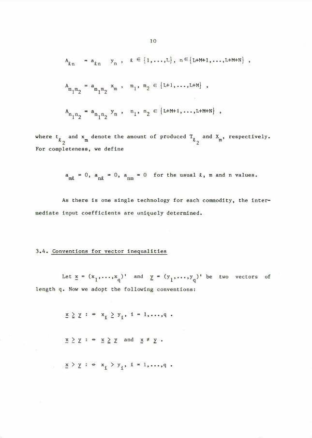
io

ARn - aRn yn 'R E 11....,L}, nE{LfM.F1,...,LtMfN} ,

m m - am m xm , ml, m2 E{Lf1,...,LtM} ,1 2 1 2

An n~ an n yn ' nl, n2 E {LtMf1,...,LtMtN} ,1 2 1 2

where tR and xm denote the amount of produced TR and Xm, respectively.2 2

For completeness, we define

a~ - 0, a~ ~ 0, anm - 0 for the usual R, m and n values.

As there is one single technology for each commodity, the inter-

mediate input coefficients are uniquely determined.

3.4. Conventions for vector inequalities

Let x-( xl,...,xq)' and y-(yl,...,yq)' be two vectors of

length q. Now we adopt the following conventions:

x~ y: A xi ~ yi, i a 1,...,q .

x~~ : p x~~ and x~ Y.

x i y: p xi i yi, i- 1,...,q .

11

4. Development of the decision model: the sectors 'End products' and

'Intermedíate products', with multiple technologies

4,1. Introduction

In this chapter a L(inear) P(rogramming) framework is proposed

that generalizes the input-output model of a firm by allowing multiple

technologies for products. The sector TS is not included here; the firmconsists of intermediate and end product divisions.

Before the actual development of the model is presented, some

remarks on the sectors 'primary input' and 'final output' are in order,

and the notion of technology is more thoroughly investigated.

The chapter is concluded with a section devoted to certain propertíes of

the model.

4.2. Primary input; final output

Suppose there are K different primary input categories (like raw

materials, labour, etc.) to be denoted by B1,...,BK. Because of the

linearity assumption, the amount of primary input involved in the pro-

duction of some product (e.g. Xm), is a fixed proportion of xm, the pro-

duced amount of }~. Hence, if Bkm denotes the flow of Bk towards D~, we

have the formula

B~-b~xm

12

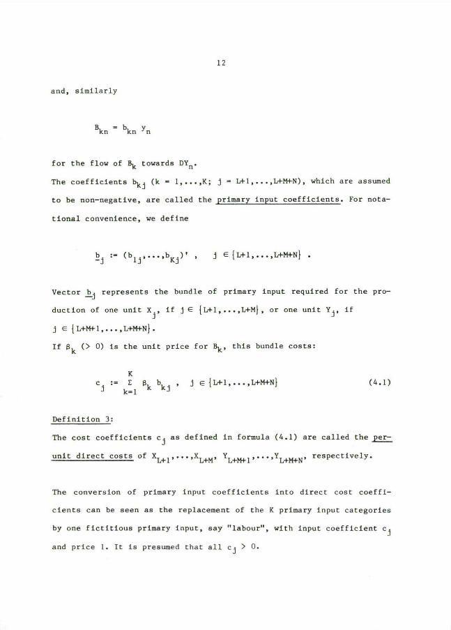
and, similarly

Bkn 3 bkn yn

for the flow of Bk towards DYn.

The coefficients bk~ (k ~ 1,...,K; j 3 Lt1,...,LfMtN), which are assumed

to be non-negative, are called the primary input coefficients. For nota-

tional convenience, we define

b~ :- (b1~,...,bK~)' , j E {Lt1,...,Lt-MtN} .

Vector b~ represents the bundle of primary input required for the pro-

duction of one unit X~, if j E{Lt1,...,LtM}, or one unit Y~, if

j E { L~-Mf 1, . . . , LtMtN } .

If sk (~ 0) is the unit príce for Bk, this bundle costs:

Kc :- E gk bk , j E{Lf1,...,LtMfN}j k-1 ~

(4.1)

Definition 3:

The cost coefficients c~ as defined in formula (4.1) are called the per-

unit direct costs of XLtl'~~~'XLfM' YLtMfl' "~'YLtMtN' respectively.

The conversion of primary i nput coefficients into direct cost coeffi-

cients can be seen as the replacement of the K primary input categories

by one fictitious primary ínput, say "labour", wíth input coefficient c~

and price 1. It is presumed that all c~ ~ 0.

13

With respect to the sector 'final output' we presume a non-nega-tive outside demand dn for every end product Yn. We denote the final

demand vector ~inal as follows:

,afinal '- dLfMfl'...'dLtMtN) .

4.3. Technology

Replace every element of the compound matrix A, defined as

A :- ó ~AN , dimensions ( M-~N) x (MfN) ,NN

by its corresponding intermediate input coefficient. We obtain a matrix

A of the same structure, but independent of the actual production

volume. Partition A in columns, i.e.

A a(aL-~1 ~'-~ ~ aLfM ~aLtMtl I''' ~ aLtMfN)

where aj :- (aLt1,j,...,aLfMfN,j)~' ~ E {Lf1,...,L-i.MfN}.

Definition 4:

The columnvector (am,bm)' is called the technology column for product

~, m E {Lt1,...,LfM}.

The columnvector ( a',b')' is called the technology column for product-n -n

Yn, n E {LfMf1,...,LtMtN}.

14

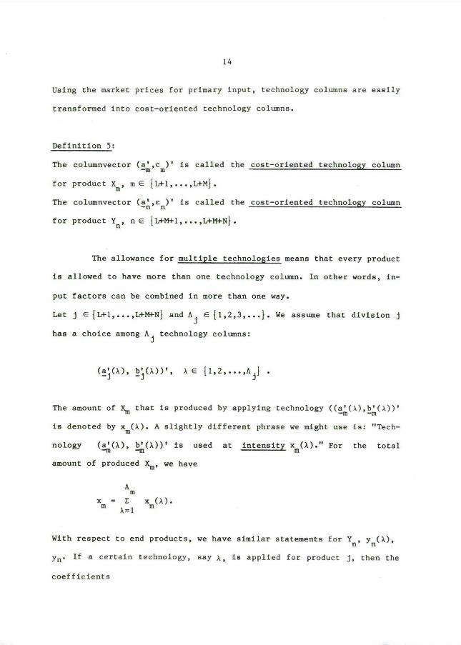
Using the market prices for primary input, technology columns are easily

transformed into cost-oriented technology columns.

Definition 5:

The columnvector ( am,cm)' is called the cost-oriented technology column

for product X, m E {Lf1,...,LfM}.m

The colvmnvector ( an,cn)' is called the cost-oriented technology columnfor product Y, n E {LfMt1,...,LfMfN}.n

The allowance for multiple technologies means that every product

is allowed to have more than one technology column. In other words, in-

put factors can be combined in more than one way.

Let j E{Lt1,...,LtMfN} and Aj E{1,2,3,...}. We assume that division j

has a choice among Aj technology columns:

(a~(a), b~(a))', .1 E {1,2,...,Aj} .

The amount of l~ that is produced by applying technology ((am(a),b~(a))'

is denoted by xm(,1). A slightly different phrase we might use is: "Tech-

nology (am(a), bm(a))' is used at intensity xm(~)." For the total

amount of produced Xm, we have

Amx a E x (a).m ~zl m

With respect to end products, we have similar statements for Y, y(a),n nyn. If a certain technology, say a, i s applied for product j , then the

coefficients

15

aij(a), i,j E {Lt1,...,Li~AftN} ;

bkj(a), k E{1,...,K}, j E{Lt1,...,LtM-FN} ;

cj(a), j E {L-1-1,...,LfM-F.N}

are the correspondíng intermediate input, primary input and per-unitdirect cost coefficients, respectívely.

In section 2.1 we have íntroduced the notion of a subset of as-signed technologies (cf. definition 1). From a more formal point ofview, each subset of assigned technologies can be characterized by avector

~ ~ ~~

~ '- ~Ltl' "''~LtM-FN) '

~ ~where aL}j E{ 1,...,AL}j} for j s 1,...,M-fN. Vector a contains one

technology index per product and hence determines one technology column

(a~(aj). bj(aj))'

for each product.

We define

A(a~) '~ (aLtl(~Ltl) ~ "' I aLtM-HN ( ~LtM-F-N))

so A(~~) is the matrix of intermediate input coefficients of assigned

technologies as characterized by ~~,

Similarly,

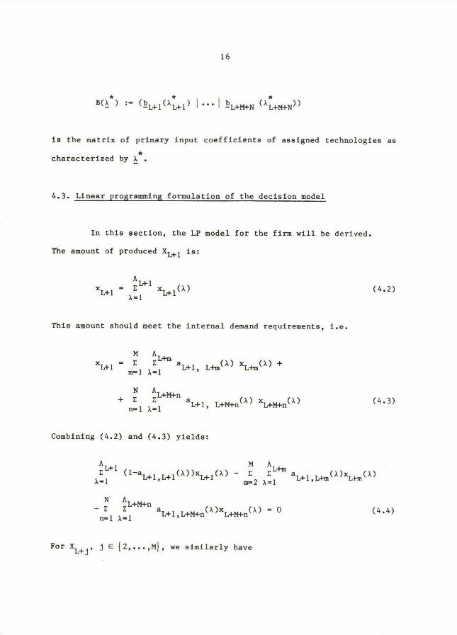
16

B(~~) '3 (bLfl(~Ltl) I " 'I bLtMtN (~LtMtN))

is the matrix of primary input coefficíents of asaigned technologies as~characterized by a .

4.3. Linear programming formulation of the decision model

In this section, the LP model for the firm will be derived.

The amount of produced XLtI is:

ALflxLfl ~ ~E1 XL-~1(~)

This amount should meet the internal demand requirements, i.e.

M A L~

xLfl - m~l a~l aLtl, L.1-m(a) xL~(a) f

f EELfMfn a

nal a~l L~-1, L~-Mtn(~) xLfMfn(~)

Combining ( 4.2) and (4.3) yields:

(4.2)

(4.3)

~Ltl(1-aLf1,Lt1(~))xLtl(a) - E EL~ aLt1,L~-m(a)xL~-m(~)

a~l m~2 aal

- E E LtM-Fn a

n~l aal Lt1,LfMtn(~)xLtM-Fn(~) - C (4.4)

For XL}j, j E{2,...,M}, we símilarly have

17

EL}j (1-a ( a))x (7~) - E EL~ a (a)x (a)~31 Lfj,Lfj L-F j m-1 a-1 Lfj , Lim L~-mm~ j

- ~ ~ LtM4.n a

n-1 ~-1 Lt1,LtMtn(~)xLfMfn(~) - C (4.5)

For end products, there are no "back deliveries" to the IP sec-

tor. Hence

(a) - 0, n- 1,...,N, m- 1,...,M, ~- 1,...,A .aLfMtn, L~-m L~-m

In order to meet internal and external demand, it should hold that,

j E {1,...,N}:

~LfMtj(1-aLfMfd(1))YLfMf~(a)- EELtM-F-naLtMfj,LtMtn(~)YLfMfn(~)

a.1-1 n-1 a~l

n~ j

- dLfMfj

The costs of production are equal to

(4.6)

E EL~cLi-m(a)xlrHm(a) f E

ELfMfncLfMfn(x)YLtM-Hn(a)

(4.7)m-1 a-1 n-1 a-1

Now recall the Central Problem (cf. section 2.2). Within thecontext of a firm without a TS sector, the Central Problem reduces to

the question:

"Given a constant final demand for end products and given constant

prices for primary input, which subset of assigned techologies will lead

to minimal total costs for the firm as a whole?"

18

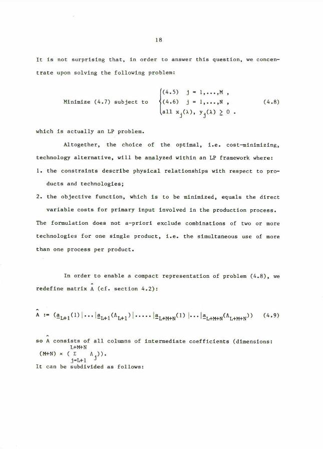
It is not surprising that, in order to answer this question, we concen-

trate upon solving the following problem:

(4.5) j L 1,...,M ,Minimize (4.7) subject to (4.6) j- 1,...,N , (4.8)

all xj(a), yj(a) ~ 0 .

which is actually an LP problem.

Altogether, the choice of the optimal, i.e. cost-minimizing,

technology alternative, will be analyzed within an LP framework where:

1. the constraints describe physical relationshipe with respect to pro-

ducts and technologies;

2. the objec[ive function, which is to be minimized, equals the direct

variable costs for primary input involved in the production process.

The formulation does not a-priori exclude combinations of two or more

technologies for one single product, i.e, the simultaneous use of more

than one process per product.

In order to enable a compact representation of problem (4.8), we

redefine matrix A(cf. section 4.2):

A :z (a (1)~...la ( A )I.....la ( 1) ~...la (A )) (4.9)-Lf1 Lf1 Lt1 LfMi-N LfMtN LtMtN

so A consists of all columns of intermediate coefficients (dimensions:LfMfN

( Mi-N ) x ( E A ) ) .j-L-F1 j

It can be subdívided as follows:

19

A - where TiN

"-NN

LfMis an M x( E Aj) matrix

j~Lf 1

LfMtNis an M x( E Aj) matrix

j~LtMf 1

LtMfNis an N x ( E Aj) matrix

j~LtMf l

Furthermore, a"generalízed identity matrix" I is required:

I :~ diag(1~), j 3 1, . ,MfN

where 1~ :- (1,...,1) is a row vector of length AL}j, with all elementsequal to 1.

So I is of the same dimensions as A. Matríx I looks like:

Now define

x :~ (xLfl(1),...,xLfl(ALfl)~....xLtM(1),...~xLtM(ALtM))' ~

Y ~3 (yLtMfl(1),...~YLtMfl(ALfMtl)'....YL-fiMfN(1)~...,YLtMtN(ALf-MfN))~ ~

z . (x'~Y')' .

x, ~ and z may be referred to as the intensity vectors of the IP sector,

the EP sector and the whole firm, respectively.

Finally,

20

~x 's (cLtl(1),...~cLtl(ALtl)~...~cLtM(1),...~cLtM(ALtM)) .

c' :~ (c (1)~-.-~c (A )....,c ( 1),...,c (A )) .-y LtMtl LtMtl LtMtl LtMtN LtMtN LtMtN

c' . (c' c') ..- -x -y

The LP problem (4.8) can be written as

Minimize c' z

s.t. (I-A) z ~ (0', dfinal)~z ~ 0

Using matricea of the same form as I, namely

IM :~ diag(lm), m ~ Lt1,...,LtM ,

IN :s diag(ln), n - L-I-Mt1,...,LtMtN ,

(4.10)

where 1~ :~ (1,...,1) is a row vector of length ALt~, with all elements

equal to 1(j E{ 1,...,MtN}), we can give a more "partitioned" represen-

tation of (4.10), i.e.

Minimize c' x t c' y-x - -y -

s.t. (IMA~)x - AMN Y s 0

(IN-ANN)Y i afinalall elements of x, y~ 0.

(4.11)

Note that in the LP formulation, matrix g which is defined as

zi

B :- (bLtl(1)~~-~IbLtl(ALtl)I.....~bLtMtN(1)I...IbLfMtN(AL~-MfN))

and hence consists of all columns of primary input coefficients, is im-

plicítly present, because

c' - 6' B

(Recall that ~' -(g1,...,SK) contains the unit prices for primary in-

put.)

4.5. Properties of the LP model

Definition 6:

Let A be a square matrix with entries ai, ~ 0. Matrix A will be calledJ -

feasible iff

d ~ [(I-A)z - d] .d ~ 0 z ~ 0 - -

Definition 7:

Let B be a square matrix of the form

B- sI-A, s~ 0, all entries of A~ 0.

Let p(A) be the spectral radius of A.

z2

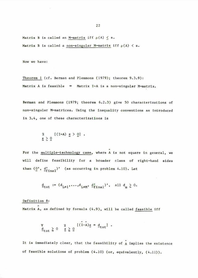
Matrix B is called an M~atrix iff p(A) ~ s.

Matrix B is called a non-singular M-matrix iff p(A) ~ s.

Now we have:

Theorem 1(cf. Berman and Plemmons (1979); theorem 9.3.9):

Matrix A is feasible p Matrix I-A is a non-singular M-matrix.

Berman and Plemmons (1979; theorem 6.2.3) give 50 characterizations of

non-singular M-matrices. Using the inequality conventions as introduced

in 3.4, one of these characterizationa is

3 [ ( I-A) z ~ 0 ] .z ~ 0 - -

For the multiple-technology case, where A is not square in general, we

will define feasibility for a broader class of right-hand sides

than (0'~ afinal)~ (as occurring in problem 4.10). Let

atot '~ (dLtl'"''dLfM' afinal)~' all d ~ 0.m -

Definition 8:

Matrix A, as defined by formula (4.9), will be called feasible iff

y g [(I-A)z ~ atot] 'atot ~ 0 z ~ 0

It is immediately clear, that the feasíbílity of A implies the existence

of feasible solutíons of problem (4.10) ( or, equivalently, (4.11)).

23

~Let a represent some subset of assigned technologies and form the cor-~

responding A(a ) (cf. section 4.3).

Theorem 2:~

If A(a ) is feasible, i n the sense of definítion 6, then A i s feasible,in the sense of definition 8.

Proof:~Let dtot ~ 0. Then (I-A(~ ))z - dtot has a non-negative solution. This

solution is easily extended [o a non-negative solution of (I-A)z - dtot~

0

Now we will cite a theorem due to Cassels (1981) whicti was ori-ginally proved for the case with just one primary input. Nevertheless,

it also applies here if we suppose that the initial K primary input

categories of our model are replaced by one fictitious primary input

(cf. section 4.1).

Furthermore, internal prices p ,...,p for XLfl LfMfN Lfl'' ~ ~'XLtM'

YLfMfI'"~'YLfMfN' respectively, play a crucial role in the following

definition and theorem:

Definition 9:

Under a certain príce p' -(pLtl'~~~'pLfMtN)' a technology column,(a~(a), b~(a))' or (aj(a), c~(a))', is said to

24

make a loss if p' aj(a) ~ c~(a) ,

break even if p'a~(a) ~ c~(a) ,

make a profit if p'a~(a) ~ cj(a) .

Theorem 3(Cassels (1981); chapter 5, theorem 2.3):

Consider the following statements:

(i) there exists an intensity vector z~ 0, such that (I-A)z ~ 0;

(ii) there exists a price vector ~~ 0, such that for every product

there is a technology column that does not make a loss;

(a) A is feasible (in the sense of definition 8);

(b) there exists a price vector v~ 0 such that no technology column

makes a profit; for every product j there is a technology column~

a3(a~) which breaks even, under this price v;~

(c) for every demand vector dtot ~ 0, a combination of the a~(a~)

only, can produce dtot efficiently, i .e. against minimal to[al

costs. Moreover, these minimal costs are equal to v'dtot~Now it holds that:

(i) p (ii), and

(1) v (ii) ~ (a), ( b), (c).

From theorem 3, we can deduce several results:

1) The implication (i) ~(c) says in particular:

(i) ~{ there exists a subset of assigned technologies,~represented by a ~

such that the corres ondin ~P g A(a ) is feasible}.

25

Of course, (a) ~ (i), so:~ ~(a) ~{there exists a a such that A(~ ) is feasible}.

Combining this with theorem 2 yields

Theorem 4:

A is feasíble p~ ~there exists a a such that A(a ) is feasible.

2) Statement (b) in theorem 3 expresses that

v'a~(a) ~ cj(a)~ J- Lf1,...,LfM-FN, a- 1,...,A.,- - - ~

equivalent with

v'(I-A) ~ c' ,

so: v is dual feasible ( see later part of this section: problem (4.12)).

In particular:

so

`d H,~ [~'a:(a~:) - c-(~~) ] ,j E{Lf1,...,LfM-FN} aj E{1,...,Aj} -

~ ~v'(I-A(a )) - (c )' .

J J J J

~with A(a ) as usual and c~ - (c (a~ ) ,...,c ( ~~ ))~ ,

- Lfl Ltl LtM-FN LtM-FN~ ~

Apparently A(a ) is feasible, so that I-A(a ) is non-singular. Hence

v' - (c~)' (I-A(a~))-1 .

26

3) From statement (c), we conclude that v is even dual optimal.

As for ever demand vector dtot' the optimal costs are equal to v'dtot'this price vector v is uniquely determined.

Nevertheless, it is not necessarily true that the dual optimum is uni-

quely determined. E.g., it is true that if there is a unique but degene-

rate primal optimum, then the dual optimum is not uniquely determined.

On the other hand, if at least one primal optimum is non-degenerate,

then there exists exactly one dual optimum (namely v!). See Papatimi-

triou and Steiglitz (1982; chapter 3, exercises 6,7).

We conclude this section with some remarks on the dual of pro-

blem (4.10), i.e.

where

Minimize d'P

s.t. (I-A)' p ~ c

d' .~ (0', afinal)

(4.12)

For convenience, assume that there is a unique dual optimum v. If we

interprete its components vLfl'~~~'~LtMtN as prices for XLfI'~~~'XLtM'

YLfMfI''"'YLfMfN respectively, the following verbalization of the dual

problem is in order:

"Choose prices ~Ltl'~~~'~LfMfN that maximize the returns d'v, subject to

the restriction that for every product the price may not exceed the unit

cost of that product under the optimal technology."

From (4.12) it is seen that the rows of the dual are of the form:

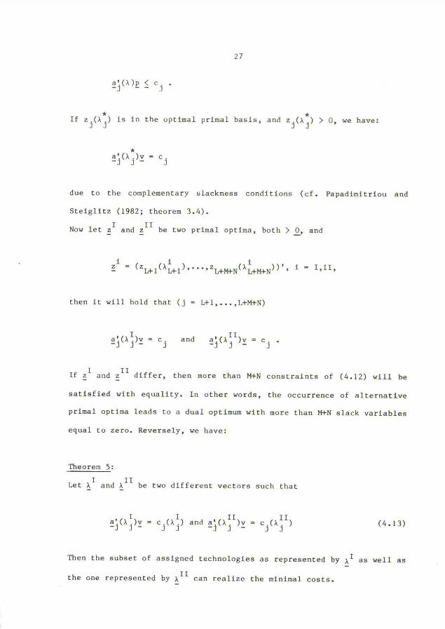
27

a~(a)P ~ cj .

~ ~If zj(aj) is in the optimal primal basis, and zj(aj) ~ 0, we have:

~aj(aj)v - cj

due to the complementary slackness conditions (cf. Papadimitriou and

Steíglitz (1982; theorem 3.4).

Now let zI and zII be two primal optima, both ~ 0, and

zi - (zLfl(~Lfl)'...'zLtMfN(~LfM-FN))'. i - I,II,

then it will hold that (j - Lt1,...,LfMfN)

'(aI)v - c. and a!(~I1)v - c. .aj j- J -J J- J

If zI and zII differ, then more than MfN constraints of (4.12) will be

satisfied with equality. In other words, the occurrence of alternativeprimal optima leads to a dual optimum with more than M-fN slack variables

equal to zero. Reversely, we have:

Theorem 5:

Let aI and aII be two different vectors such that

a'.(aL)~ - c.(ai) and a!(aII)~ - c.(aII)'J J- J J -J J - J J(4.13)

Then the subset of assigned technologies as represented by ~I as well asthe one represented by ~II can realize the mínimal costs.

28

Proof:

From ( 4.13), we see that there exiats a price vector ~~ 0(viz. ~- v)

such that

P'(I-A(aI)) - c'(aI)

where c'(aI) :~ (c1,.F1(~Ltl)'....cLfMfN(~LfMfN))~ ~ 0' .

Using theorem 6.2.3 from Berman and Plemmons (1979) yields the result

that I-A(aI) ia a non-aingular M-matrix. Hence, A(aI) is feasible (cf.

theorem 1).

Now consider the LP problem:

Minimize c'(aI)y

s.t. (I-A(aI))Y - d

~ ~ 0

The optimal solu[ion value will equal v'd, while the optimal solution YI

is easily extended to an (optimal!) solution of the original LP problem

(4.10). Analoguously, A(aII) leads to a different optimal solution of

the original LP problem (4.10).

So A(aI) as well as A(~II) can realize minimal costs. ~

29

5. The incorporation of technical services

5.1. Introduction

It is our aim to extend the model of chapter 4 with a TS sector.

As noted in chapter 3, we will account for L different technical servi-

ces T1,...,T~,...,TL.

- They are demanded for by the product divisions, and

- they can also be bought externally instead of producing them internal-

ly.

If (some of) these services are bought from external suppliers, the firm

avoids the variable as well as the fixed costs of internal production.

Instead, the firm íncurs variable costs due to the per-unit price for

externally supplied services.

From now on, the extension of our decision model with a TS sec-

tor in the above described sense will briefly be referred to as: "the

incorporation of technical services". First of all, a few notational

extensions are in order. Then we treat the case with a constant demand

for technical services. Finally, the ultimate decision model can be pre-

sented, wherein the demand for technical services is a(linear) function

of the divisions production intensities.

5.2. Make-or-buy decisions

For every TS, there are two mutually exclusive possibilities:

1) TR is produced internally.

The per-unit direct costs of TR are cR(in).

30

The amount of internally produced TR is tR(in).

If tR(in) ~ 0, then the firm incurs a fixed cost equal to CR(fix).

Hence, the total cost of internal production is:

cR(in)tR(in) f CR(fix), tR(in) ~ 0.

Internal production of TR requirea an amount aiRtR(in) of Ti,

i E{1,...,L}, where aiR ~ 0. Such a rate aiR is again referred to as an

intermediate input coefficient. We define the matrix ALL(in) as follows:

LL(in) . (al ... aL)

where aR :~ (a1R,...,a~)', R E {1,...,L}.

It is presumed that !~L(in) is feasible ( cf. definition 6).

2) TR is bought externally.

The amount of externally bought TR is tR(ex).

The firm incurs a variable cost equal to

cR(ex) tR(ex)

where cR(ex) is the per-unit external price of TR. Some TS that is

bought externally, does not require certain amounts of other TS-ses.

31

5.3. 'Phe case wi[h a cona[aut dc~mand for [echnical services

Definition 10:

The net demand for TR is defined as the amount of TR required by the IP

and EP sector. Notation: tR. We require t~ ~ 0.

If tR is constant for every TS, the Central Problem splits into

two independent subproblems, namely the problem of finding the optimal

divisional technologies and the problem of finding the optimal internal-

external alternative. This section trea[s the latter problem. To this

end, we can simply adopt the approach as introduced by Manes, Park and

Jensen (1982), which leads to a míxed-integer programming formulation.

We refer to Manes et. al. for the actual development of the model. Fur-

thermore, these authors provide for a historical overview of the

research of the so-called reciprocal service-cost problem. Up to their

contribution, especially the aspect of (eventually avoidable) fixed

cos[s had received little attention in the literature.

Altogether, for the problem of finding the op[imal internal-ex-

ternal alternative wíth all tR constant, we propose the following mixed-

integer programmíng framework:

32

L L LMinimize E cR(ex)tR(ex) f E cR(in)tR(in) t E CR(fix)dR

R-1 Rsl Ral

Ls.t. tR(ex) t ( 1-aRR(in))tR(in) - E aRj(in)t~(in) r tR, R - 1,...,L

j-1

tR(in) - M dR ~ 0, R a 1,...,L

all dR 0-1 variables, all tR(in), tR(ex) ~ 0

Here M is a large number that guarantees: tR(in) ~ 0~ óR ~ 1.

The following definitions enable a more compact formulation of this pro-

blem.

Let:

t(ex) :~ (tl(ex),...,tL(ex))' ,

t(in) :~ (tl(in),...,tL(in))' ,

~t . (t1,...~tL ~

d:~ (ó1,...,dL)', all dR 0-1 variables,

c'(ex) :~ (cl(ex),...,cL(ex)) ,

c'(in) :s (cl(in),...,cL(in)) ,

C'(fix) :a (C1(fix),...,CL(fix)) .

33

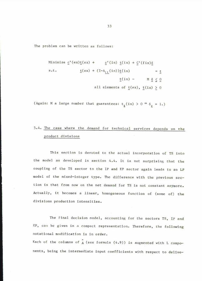
The problem can be written as follows:

Minimize c'(ex)t(ex) f c'(in) [(in)

s.t.

all elements of

t(ex) f (I-ALL(in))t(in)

t(in)

t C'(fix)d

- t

- M d ~ 0

t(ex), t(in) ~ 0

(Again: M a large number that guarantees: tR(in) ~ 0~ d~ - 1.)

5.4. The case where the demand for technical services depends on the

product divisions

This section ís devoted to the actual incorporation of TS into

the model as developed in section 4.4. It is not surprising that the

coupling of the TS sector to the IP and EP sector again leads to an LP

model of the mixed-integer type. The difference with the previous sec-

tíon is that from now on the net demand for TS is not constant anymore.

Actually, it becomes a linear, homogeneous function of (some of; the

divisions production intensities.

The final decision model, accounting for the sectors TS, IP and

EP, caii be gíven in a compact representation. Therefore, the following

notational modification is in order.

Each oE the columns of A(see formula (4.9)) is augmented with L compo-

nents, being the intermediate input coefficients with respect to delive-

34

ries from TS to IP and EP sector. Such a column aL}~(a) is of the form

(j ' 1,...,MtN):

aL}~(a) :' (a1~L~j(a)....,aL~L}~(a). aLf~(a))' .

We will not continue to write down the superscripts "new". The new A can

be subdivided as follows:

f ~, ZNthe dimensions of A~, A~, ANNremain the same,

A s

0-TTN

„ LfMALM is an L x ( E A~) matrix,

j~Lf 1

„ LfMfNALN is an L x( E Aj) matrix.

jaL~-Mf 1

In figure 3, the ultimate M(ixed) I(integer) P(rogramming) model is pre-

sented.

6. Summary

In this paper, we have developed a model for the firm including

multiple technologies, and "make-or-buy" decisions. Though we start in a

typical input-output setting, we end up in a mixed integer programming

formulation.

With respect to the "make-or-buy" aspect, there is a correspon-

dence with recent literature, viz. Manes et. al. (1982). As noted in

this article, there are practical limitations on the size of effective

35

integer programs. A theoretical difficulty is that duality theory for

integer programming is considerably weaker than it is for ordinary LP.

In future research, the issue of common cost allocation is to be

incorporated ín order to obtain a so-called "integral model of the

Eirm".

36

References

Berman A. and R.J. Plemmons (1979). Non-negative matrices in the mathe-

matical sciences. New York: Academic Press.

Cassels, J.W.S. (1981). Economics for Mathematicians. Cambridge: Univer-

sity Press, London Mathematical Society Lecture Note Series 62.

Halem, C. van (1982). Input-output bedrijfsmodellen. 's-Gravenhage:

Drukkerij J.H. Pasmans B.V., in Dutch.

Livingstone, J.L. ( 1969). "Input-output analysis for cost accounting,

planning and control", The Accounting Review 44, 48-64.

Leontief, W. (1936). "Quantitative input-output relations in the econo-

mic system of the United States", The Review of Economics and Statis-

tics.

Manes, R.P., S.H. Park and R. Jensen (1982). "Relevant costs of interme-

diate goods and services", The Accounting Review 57, no. 3, 594-606.

Papadimitriou, C.H. and K. Steiglitz (1982). Combinatorial optimization:

algorithms and complexity. New Yersey: Prentíce Hall Inc., Englewood

Cliffs.

Smits, H.A. and P.A. Verheyen (1976). "The development of a budgeting

model", in C.B. Tilanus (ed.), Quantitative methods in budgeting. Lei-

den: Nijhoff.

37

To

FromGS TS IP EP final

output

GS

TS

IP

EP

primaryinput

Figure 1: General input-output table; only EP sector delivers to

'final output'.

38

To TS IP EP

From 1, . . . , L Lf 1 , . . . ,LfM LtMf 1, . . . , LfMfN

1

TS ~ ALL ALM ALN

L

IrE 1

IP ~ A~ A~

LfM

LtMtl

EP ~ ANNLfMfN

Figure 2: Input-output table for corporate model, sectors 'pri-

mary input' and 'final output' deleted.

Cross X symbolizes the absence of certain types of

deliveries.

39

Minimize

c'(ex)t(ex)f

subject to

c'(in) t(in)f cX xt cy ytC'(fix)d

t(ex)t(I-t~L(in))t(in)- ~ x- A~~ Y - 0

( IM-A~) x- AMN ~ - 0

t(in) -M 6 C 0

all elements of x, y, t(ex), t(in) ~ 0

d-(61,...,dL)', all d~ 0-1 variables

M is a large number that guarantees: tR(in) ~ 0~ dR - 1

Figure 3: MIP-model, including EP, IP and TS sector

i

IN 1983 REEDS VERSCAENEN

126 H.H. TigelaarIdentífícation of noisy linear systems with multiple arma inputs.

1"L7 J.P.C. KleíjnenStatis[ical Analysis of Steady-State Simulations: Survey of RecentProgress.

128 A.J. de ZeeuwTwo notes on Nash and Information.

129 H.L. Theuns en A.M.L. Passier-GrootjansToeristische ontwikkeling - voorwaarden en systematiek; een selec-tief literatuuroverzicht.

130 J. Plasmans en V. SomersA Maximum Likelihood Estimation Method of a Three Market Disequili-brium Model.

131 R. van Montfort, R. Schippers, R. HeutsJohnson SU-transformations for parameter estimation in arma-modelswhen data are non-gaussian.

132 J. Glombowski en M. KrugerOn the R81e of Distribution in Different Theories of CyclicalGrowth.

133 J.W.A. Vingerhoets en H.J.A. CoppensInternationale Grondstoffenovereenkomsten.Effecten, kosten en oligopolisten.

134 W.J. OomensThe economic interpretation of the advertising effect of LydiaPinkham.

135 J.P.C. KleijnenRegressíon analysis: assumptions, alternatives, applications.

136 J.P.C. KleijnenOn the interpretation of variables.

137 G, van der Laan en A.J.J. TalmanSimplicial approximation of solutions to the nonlinear complemen-tarity problem with lower and upper bounds.

ii

IN 1984 REEDS VERSCHENEN

138 G.J. Cuypere, J.P.C. Kleíjnen en J.W.M. van RooyenTeating the Mean of an Asymetric Population:Four Procedures Evaluated

139 T. Wansbeek en A. KapteynEstimation in a linear model with serially correlated errors whenobservations are missing

140 A. Kapteyn, S. van de Geer, H. van de Stadt, T. WansbeekInterdependent preferences: an econometric analysis

141 W.J.H. van GroenendaalDiscrete and continuous univariate modelling

142 J.P.C. Kleijnen, P. Cremers, F. van BelleThe power of weighted and ordinary least squares with estimatedunequal variances in experimental design

143 J.P.C. KleijnenSuperefficient estimation of power functions in simulationexperiments

144 P.A. Bekker, D.S.G. PollockIdentification of linear stochastic models with covariancerestrictiona.

145 Max D. Merbis, Aart J. de ZeeuwFrom structural form to state-space form

146 T.M. Doup and A.J.J. TalmanA new variable dimension simplicial algorithm to fínd equilibria onthe product space of unit simplices.

147 G. van der Laan, A.J.J. Talman and L. Van der HeydenVariable dimension algorithms for unproper labellings.

148 G.J.C.Th. van SchijndelDynamic firm behaviour and financial leverage clienteles

149 M. Plattel, J. PeílThe ethico-polítical and theoretical reconstruction of contemporaryeconomic doctrines

150 F.J.A.M. Hoes, C.W. VroomJapanese Business Policy: The Cash Flow Trianglean exercise in sociological demystification

151 T.M. Don}u~, G. van der Laan and A.J.J. TalmanThe (2 -2)-ray algorithm: a new simplicial algorithm to computeeconomic equilibria

111

IN 1984 REEDS VERSCKENEN (vervolg)

152 A.L. Hempenius, P.G.H. MulderTotal Mortality Analysis of the Rotterdam Sample of the Kaunas-Rotterdam Intervention Study (KRIS)

153 A. Kapteyn, P. KooremanA disaggregated analysis of the allocation of time within thehousehold.

154 T. Wansbeek, A. KapteynStatistically and Computationally Efficient Estimation of theGravity Model.

155 P.F.P.M. NederstigtOver de kosten per ziekenhuisopname en levensduurmodellen

m u u ii~ui iii ~~~uNiiinu~wiuuui u