Subelliptic Estimates and Finite Type - MSRIlibrary.msri.org/books/Book37/files/dangelo.pdf ·...
34
Several Complex Variables MSRI Publications Volume 37, 1999 Subelliptic Estimates and Finite Type JOHN P. D’ANGELO AND JOSEPH J. KOHN Abstract. This paper surveys work in partial differential equations and several complex variables that revolves around subelliptic estimates in the ∂-Neumann problem. The paper begins with a discussion of the ques- tion of local regularity ; one is given a bounded pseudoconvex domain with smooth boundary, and hopes to solve the inhomogeneous system of Cauchy– Riemann equation ∂u = α, where α is a differential form with square inte- grable coefficients and satisfying necessary compatibility conditions. Can one find a solution u that is smooth wherever α is smooth? According to a fundamental result of Kohn and Nirenberg, the answer is yes when there is a subelliptic estimate. The paper sketches the proof of this result, and goes on to discuss the history of various finite-type conditions on the boundary and their relationships to subelliptic estimates. This includes finite-type conditions involving iterated commutators of vector fields, subelliptic mul- tipliers, finite type conditions measuring the order of contact of complex analytic varieties with the boundary, and Catlin’s multitype. The paper also discusses additional topics such as nonpseudoconvex domains, Holder and L p estimates for ∂ , and finite-type conditions that arise when studying holomorphic extension, convexity, and the Bergman kernel function. The paper contains a few new examples and some new calculations on CR manifolds. The paper ends with a list of nine open problems. Contents 1. Introduction 200 2. The Levi Form 201 3. Subelliptic Estimates for the ∂-Neumann Problem 204 4. Ideals of Subelliptic Multipliers 207 5. Finite Commutator-Type 210 6. Orders of Contact and Finite Dq -type 212 7. Catlin’s Multitype and Sufficient Conditions for Subelliptic Estimates 215 8. Necessary Conditions and Sharp Subelliptic Estimates 218 9. Domains in Manifolds 220 10. Domains That Are Not Pseudoconvex 221 11. A Result for CR Manifolds 223 12. H¨ older and L p estimates for ∂ 225 13. Brief Discussion of Related Topics 226 14. Open Problems 228 References 229 199
-
Upload
duongxuyen -
Category
Documents
-
view
216 -
download
0
Transcript of Subelliptic Estimates and Finite Type - MSRIlibrary.msri.org/books/Book37/files/dangelo.pdf ·...

Several Complex VariablesMSRI PublicationsVolume 37, 1999
Subelliptic Estimates and Finite Type
JOHN P. D’ANGELO AND JOSEPH J. KOHN
Abstract. This paper surveys work in partial differential equations andseveral complex variables that revolves around subelliptic estimates in the∂-Neumann problem. The paper begins with a discussion of the ques-tion of local regularity; one is given a bounded pseudoconvex domain withsmooth boundary, and hopes to solve the inhomogeneous system of Cauchy–Riemann equation ∂u = α, where α is a differential form with square inte-grable coefficients and satisfying necessary compatibility conditions. Canone find a solution u that is smooth wherever α is smooth? According to afundamental result of Kohn and Nirenberg, the answer is yes when there isa subelliptic estimate. The paper sketches the proof of this result, and goeson to discuss the history of various finite-type conditions on the boundaryand their relationships to subelliptic estimates. This includes finite-typeconditions involving iterated commutators of vector fields, subelliptic mul-tipliers, finite type conditions measuring the order of contact of complexanalytic varieties with the boundary, and Catlin’s multitype.
The paper also discusses additional topics such as nonpseudoconvex
domains, Holder and Lp estimates for ∂, and finite-type conditions thatarise when studying holomorphic extension, convexity, and the Bergmankernel function. The paper contains a few new examples and some newcalculations on CR manifolds. The paper ends with a list of nine openproblems.
Contents
1. Introduction 2002. The Levi Form 2013. Subelliptic Estimates for the ∂-Neumann Problem 2044. Ideals of Subelliptic Multipliers 2075. Finite Commutator-Type 2106. Orders of Contact and Finite Dq-type 2127. Catlin’s Multitype and Sufficient Conditions for Subelliptic Estimates 2158. Necessary Conditions and Sharp Subelliptic Estimates 2189. Domains in Manifolds 220
10. Domains That Are Not Pseudoconvex 22111. A Result for CR Manifolds 22312. Holder and Lp estimates for ∂ 22513. Brief Discussion of Related Topics 22614. Open Problems 228References 229
199

200 JOHN P. D’ANGELO AND JOSEPH J. KOHN
1. Introduction
The solution of the Levi problem during the 1950’s established the fundamen-tal result in function theory characterizing domains of holomorphy. Suppose thatΩ is a domain in complex Euclidean space Cn. The solution establishes that threeconditions on Ω are identical: Ω is a domain of holomorphy, Ω is pseudoconvex,and the sheaf cohomology groups Hq(Ω, O) are trivial for each q ≥ 1. The firstproperty is a global function-theoretic property, the second is a local propertyof the boundary, and the third tells us that certain overdetermined systems oflinear partial differential equations (the inhomogeneous Cauchy–Riemann equa-tions) always have smooth solutions.
After the solution of the Levi problem, research focused upon domains withsmooth boundaries and mathematicians hoped to establish deeper connectionsbetween partial differential equations and complex analysis. This led to thestudy of the Cauchy–Riemann equations on the closed domain and to manyquestions relating the boundary behavior of the Cauchy–Riemann operator ∂to the function theory on Ω. We continue the introduction by describing thequestion of local regularity for ∂, and how its study motivated various geometricnotions of “finite type”.
Suppose that Ω is a bounded domain and that its boundary bΩ is a smoothmanifold. We define ∂ in the sense of distributions. Let α be a differential(0, q) form with square-integrable coefficients and satisfying the compatibilitycondition ∂α = 0. What geometric conditions on bΩ guarantee that we cansolve the Cauchy–Riemann equation ∂u = α so that the (0, q−1) form u mustbe smooth wherever α is? Here smoothness up to the boundary is the issue.
One approach to regularity results is the ∂-Neumann problem. See [Follandand Kohn 1972; Kohn 1977; 1984] for extensive discussion. Let L2
(0,q)(Ω) denotethe space of (0, q) forms with square-integrable coefficients. The ∂-Neumannproblem generalizes Hodge theory; careful attention to boundary conditions isnow required. Under certain geometric conditions on bΩ, Kohn constructed anoperator N on L2
(0,q)(Ω) such that u = ∂∗Nα gives the unique solution to ∂u = α
that is orthogonal to the null space of ∂ on Ω. This is called the canonical solutionor the ∂-Neumann solution. In particular the Neumann operator N exists onbounded pseudoconvex domains. What additional geometric conditions on bΩguarantee that N is a pseudo-local operator, and hence yield local regularity forthe canonical solution u? By local regularity we mean that u is smooth whereverα is smooth. We shall see that pseudolocality for N follows from subellipticestimates.
Kohn [1963; 1964] solved the ∂-Neumann problem on strongly pseudocon-vex domains in 1962. Subsequent work by Kohn and Nirenberg [1965] exposedclearly the subelliptic nature of the problem. Local regularity holds on stronglypseudoconvex domains because there is a subelliptic estimate; in this case onecan take ε equal to 1
2in Definition 3.4 of this paper. Local regularity follows

SUBELLIPTIC ESTIMATES AND FINITE TYPE 201
from a subelliptic estimate for any positive ε (see Theorem 3.5); this led Kohn toseek geometric conditions for subelliptic estimates. For domains in two dimen-sions he introduced in [1972] a finite-type condition (called “finite commutator-type” in this paper) enabling him to prove a subelliptic estimate. Greiner [1974]established the necessity of finite commutator-type in two dimensions. Thesetheorems generated much work concerned with intermediate conditions betweenpseudoconvexity and strong pseudoconvexity. Different analytic problems leadto different intermediate, or finite-type, conditions on bΩ. After contributionsby many authors, Catlin [1983; 1984; 1987] completely solved one major problemof this kind. He proved that a certain finite-type condition is both necessary andsufficient for subelliptic estimates on (0, q) forms for q ≥ 1 for the ∂-Neumannproblem on smoothly bounded pseudoconvex domains. The finite-type conditionis that the maximum order of contact of q-dimensional complex-analytic varietieswith the boundary be finite at each point.
In this paper we survey those finite-type conditions arising from subellip-tic estimates for the ∂-Neumann problem and we indicate their relationship tofunction theory, geometry, and partial differential equations. We provide greaterdetail when we discuss subelliptic multipliers; we consider their use both on do-mains that are not pseudoconvex and on domains in CR manifolds. We indicatedirections for further research and end the paper with a list of open problems.
2. The Levi Form
We begin by considering the geometry of the boundary of a domain in complexEuclidean space and its relationship to the function theory on the domain, usingespecially the Cauchy–Riemann operator ∂ and the ∂-Neumann problem. LetΩ denote a domain in Cn whose boundary is a smooth manifold denoted bybΩ or by M . Pseudoconvexity is a geometric property of bΩ that is necessaryand sufficient for Ω to be a domain of holomorphy; for domains with smoothboundaries, pseudoconvexity is determined by the Levi form.
We recall an invariant definition of the Levi form that makes sense also forCR manifolds of hypersurface type. Thus we suppose that M is a smooth realmanifold of dimension 2n − 1 and that CTM denotes its complexified tangentbundle.
We say that M is a CR manifold of hypersurface type if there is a subbundleT 1,0M ⊂ CTM such that the following conditions hold:
1. T 1,0M is integrable (closed under the Lie bracket operation).2. T 1,0M ∩ T 1,0M = 0.3. The bundle T 1,0M ⊕ T 1,0M has codimension one in CTM .
For real submanifolds in Cn the bundle T 1,0M is defined by CTM ∩ T 1,0Cn,and thus local sections of T 1,0M are complex (1, 0) vector fields tangent to M .

202 JOHN P. D’ANGELO AND JOSEPH J. KOHN
The bundle T 1,0M is closed under the Lie bracket, or commutator, [ , ]. For CRmanifolds this integrability condition is part of the definition.
On the other hand, the bundle T 1,0M ⊕ T 1,0M is generally not integrable.The Levi form measures the failure of integrability. To define it, we denote by η apurely imaginary non-vanishing 1-form that annihilates T 1,0M ⊕ T 1,0M . WhenM is a hypersurface, and r is a local defining function, we may put η = 1
2(∂ − ∂)r.We write 〈 , 〉 for the contraction of a one-form and a vector field.
Definition 2.1. The Levi form λ is the Hermitian form on T 1,0M defined (upto a multiple) by
λ(L,K) = 〈η, [L,K]〉. (1)
The CR manifold M is called strongly pseudoconvex when λ is definite, and iscalled weakly pseudoconvex when λ is semi-definite but not definite. We saythat the domain lying on one side of a real hypersurface is pseudoconvex whenλ is positive semi-definite on the hypersurface.
We can also interpret the Levi form as the restriction of the complex Hessian of adefining function to the space T 1,0M . To see this we use the Cartan formula forthe exterior derivative of η. Because L,K are annihilated by η and are tangentto M , we can write
〈∂∂r, L∧K〉 = 〈−dη, L ∧K〉 = −L〈η,K〉+K〈η, L〉+ 〈η, [L,K]〉 = λ(L,K).
It is also useful to express the entries of the matrix λ with respect to a speciallocal basis of the (1, 0) vector fields. Suppose that r is a defining function, andthat we are in a neighborhood where rzn 6= 0. We put
T =1rzn
∂
∂zn− 1rzn
∂
∂zn.
Then 〈η, T 〉 = 1. For i = 1, 2, . . . , n− 1 we define Li by
Li =∂
∂zi− rzirzn
∂
∂zn.
Then the Li, for i = 1, 2, . . .n − 1, form a commuting local basis for sectionsof T 1,0M . Furthermore [Li, Lj ] = λijT . Using subscripts for partial derivativeswe have
λij =ri|rn|2 − rinrnr − rnrirn + rnnrir
|rn|2.
Strong pseudoconvexity is a non-degeneracy condition: if λ is positive-definiteat a point p ∈ M , then it is positive-definite in a neighborhood. Furthermorestrong pseudoconvexity is “finitely determined”: if M ′ is another hypersurfacecontaining p and osculating M to second order there, then M ′ is also stronglypseudoconvex at p. In seeking generalizations of strong pseudoconvexity thathave applications in analytic problems we expect that generalizations will beboth open and finitely determined conditions.
SUBELLIPTIC ESTIMATES AND FINITE TYPE 203
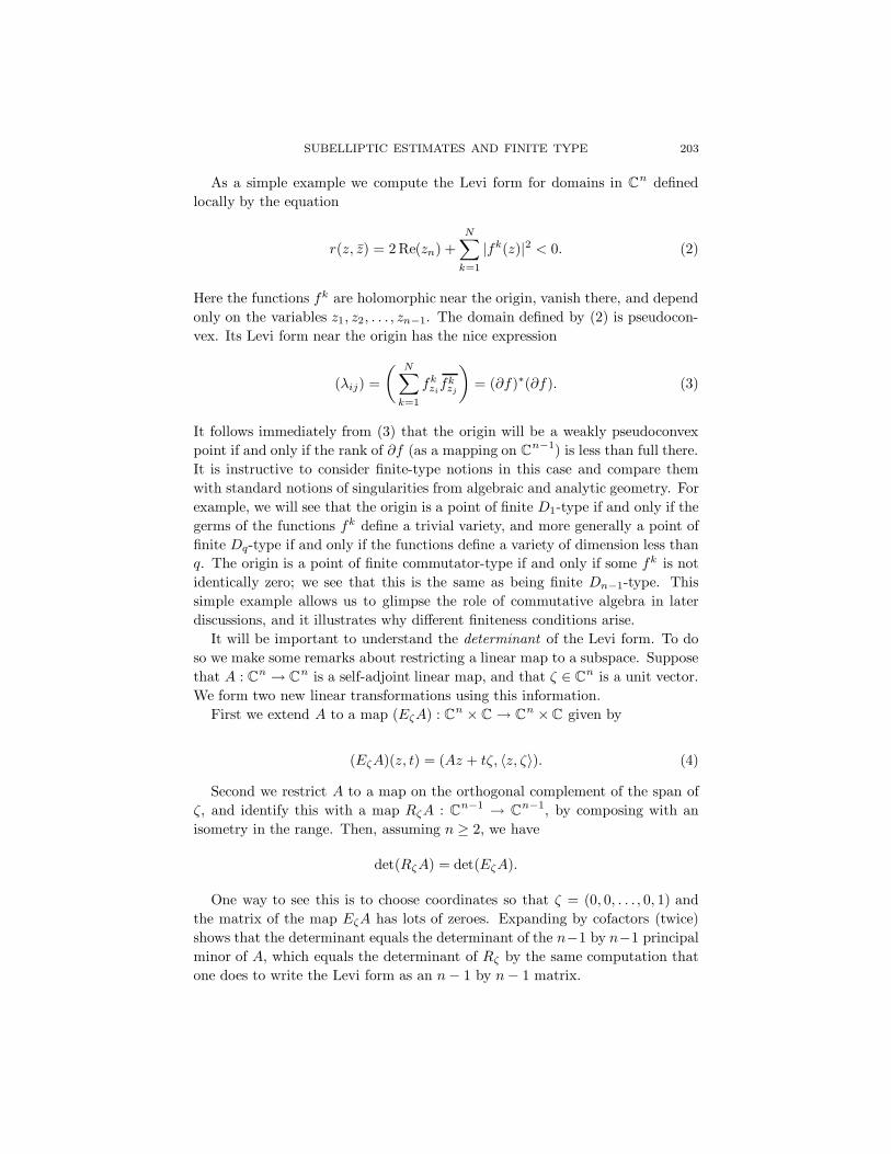
As a simple example we compute the Levi form for domains in Cn definedlocally by the equation
r(z, z) = 2 Re(zn) +N∑k=1
|fk(z)|2 < 0. (2)
Here the functions fk are holomorphic near the origin, vanish there, and dependonly on the variables z1, z2, . . . , zn−1. The domain defined by (2) is pseudocon-vex. Its Levi form near the origin has the nice expression
(λij) =
( N∑k=1
fkzifkzj
)= (∂f)∗(∂f). (3)
It follows immediately from (3) that the origin will be a weakly pseudoconvexpoint if and only if the rank of ∂f (as a mapping on Cn−1) is less than full there.It is instructive to consider finite-type notions in this case and compare themwith standard notions of singularities from algebraic and analytic geometry. Forexample, we will see that the origin is a point of finite D1-type if and only if thegerms of the functions fk define a trivial variety, and more generally a point offinite Dq-type if and only if the functions define a variety of dimension less thanq. The origin is a point of finite commutator-type if and only if some fk is notidentically zero; we see that this is the same as being finite Dn−1-type. Thissimple example allows us to glimpse the role of commutative algebra in laterdiscussions, and it illustrates why different finiteness conditions arise.
It will be important to understand the determinant of the Levi form. To doso we make some remarks about restricting a linear map to a subspace. Supposethat A : Cn → Cn is a self-adjoint linear map, and that ζ ∈ Cn is a unit vector.We form two new linear transformations using this information.
First we extend A to a map (EζA) : Cn × C → Cn ×C given by
(EζA)(z, t) = (Az + tζ, 〈z, ζ〉). (4)
Second we restrict A to a map on the orthogonal complement of the span ofζ, and identify this with a map RζA : Cn−1 → Cn−1, by composing with anisometry in the range. Then, assuming n ≥ 2, we have
det(RζA) = det(EζA).
One way to see this is to choose coordinates so that ζ = (0, 0, . . . , 0, 1) andthe matrix of the map EζA has lots of zeroes. Expanding by cofactors (twice)shows that the determinant equals the determinant of the n−1 by n−1 principalminor of A, which equals the determinant of Rζ by the same computation thatone does to write the Levi form as an n− 1 by n− 1 matrix.

204 JOHN P. D’ANGELO AND JOSEPH J. KOHN
According to this result we may express the determinant of the Levi form asthe determinant of the n+ 1 by n+ 1 bordered Hessian matrix
E =
rz1z1 rz2z1 . . . rznz1 rz1rz1z2 rz2z2 . . . rznz2 rz2
......
. . ....
...rz1zn rz2zn . . . rznzn rznrz1 rz2 . . . rzn 0
. (5)
It will be convenient later to write (5) in simpler notation. To do so, weimagine ∂r as a row, and ∂r as a column. We get
E =(∂∂r ∂r
∂r 0
). (6)
Finally we remark that when the defining equation is given by (3), there is asimple formula for the determinant of the Levi form. We have
det(λ) =∑|J(fi1 , . . . , fin−1)|2,
where the sum is taken over all choices of n−1 of the functions fk, and J denotesthe Jacobian determinant in n−1 dimensions. Thus the determinant of the Leviform is the squared norm of a holomorphic mapping in this case.
3. Subelliptic Estimates for the ∂-Neumann Problem
From the introduction we have seen that the ∂-Neumann problem constructsa particular solution to the inhomogeneous Cauchy–Riemann equations. The ∂-Neumann problem is a boundary value problem; the equation is elliptic, but theboundary conditions are not elliptic. One of the most important results, due toKohn and Nirenberg, states that local regularity for the canonical solution to theinhomogeneous Cauchy–Riemann equations follows from a subelliptic estimate.In this section we define subelliptic estimates, and sketch a proof of the Kohn–Nirenberg result.
We begin by recalling the definition of the tangential Sobolev norms. We writeRm− for the subset of Rm whose last coordinate is negative. For convenience wedenote the first m− 1 components by t and the last component by r.
Definition 3.1 (Partial Fourier Transform). Suppose that u ∈ C∞0 (Rm− ).The partial Fourier transform of u is given by
u(ξ, r) =∫Rm−1
e−it·ξu(t, r) dt.
Definition 3.2. Suppose that u ∈ C∞0 (Rm− ). We define the tangential pseudo-differential operator Λs and the tangential Sobolev norm ‖‖u‖‖s by
(Λsu)(ξ, r) = (1 + |ξ|2)s/2u(ξ, r), ‖‖u‖‖s = ‖Λsu‖.
SUBELLIPTIC ESTIMATES AND FINITE TYPE 205
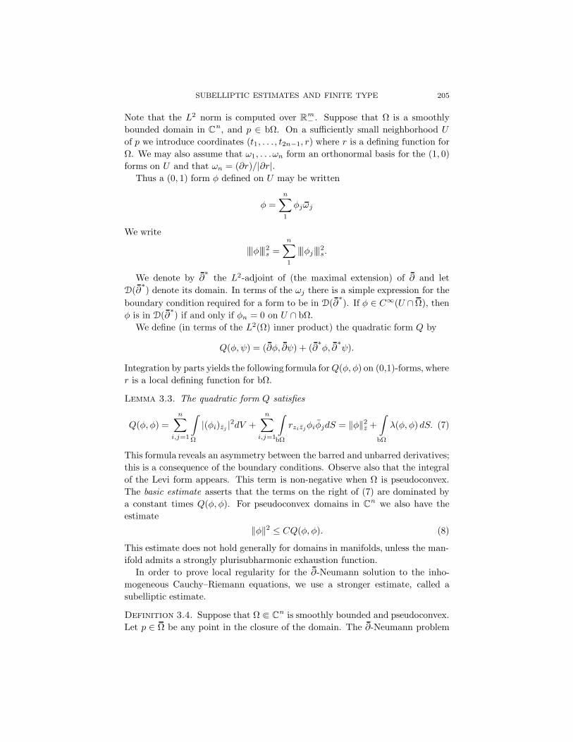
Note that the L2 norm is computed over Rm− . Suppose that Ω is a smoothlybounded domain in Cn, and p ∈ bΩ. On a sufficiently small neighborhood U
of p we introduce coordinates (t1, . . . , t2n−1, r) where r is a defining function forΩ. We may also assume that ω1, . . .ωn form an orthonormal basis for the (1, 0)forms on U and that ωn = (∂r)/|∂r|.
Thus a (0, 1) form φ defined on U may be written
φ =n∑1
φjωj
We write
‖‖φ‖‖2s =n∑1
‖‖φj‖‖2s.
We denote by ∂∗
the L2-adjoint of (the maximal extension) of ∂ and letD(∂
∗) denote its domain. In terms of the ωj there is a simple expression for the
boundary condition required for a form to be in D(∂∗). If φ ∈ C∞(U ∩Ω), then
φ is in D(∂∗) if and only if φn = 0 on U ∩ bΩ.
We define (in terms of the L2(Ω) inner product) the quadratic form Q by
Q(φ, ψ) = (∂φ, ∂ψ) + (∂∗φ, ∂
∗ψ).
Integration by parts yields the following formula forQ(φ, φ) on (0,1)-forms, wherer is a local defining function for bΩ.
Lemma 3.3. The quadratic form Q satisfies
Q(φ, φ) =n∑
i,j=1
∫Ω
|(φi)zj |2dV +n∑
i,j=1
∫bΩ
rzizjφiφjdS = ‖φ‖2z +∫
bΩ
λ(φ, φ) dS. (7)
This formula reveals an asymmetry between the barred and unbarred derivatives;this is a consequence of the boundary conditions. Observe also that the integralof the Levi form appears. This term is non-negative when Ω is pseudoconvex.The basic estimate asserts that the terms on the right of (7) are dominated bya constant times Q(φ, φ). For pseudoconvex domains in Cn we also have theestimate
‖φ‖2 ≤ CQ(φ, φ). (8)
This estimate does not hold generally for domains in manifolds, unless the man-ifold admits a strongly plurisubharmonic exhaustion function.
In order to prove local regularity for the ∂-Neumann solution to the inho-mogeneous Cauchy–Riemann equations, we use a stronger estimate, called asubelliptic estimate.
Definition 3.4. Suppose that Ω b Cn is smoothly bounded and pseudoconvex.Let p ∈ Ω be any point in the closure of the domain. The ∂-Neumann problem
206 JOHN P. D’ANGELO AND JOSEPH J. KOHN
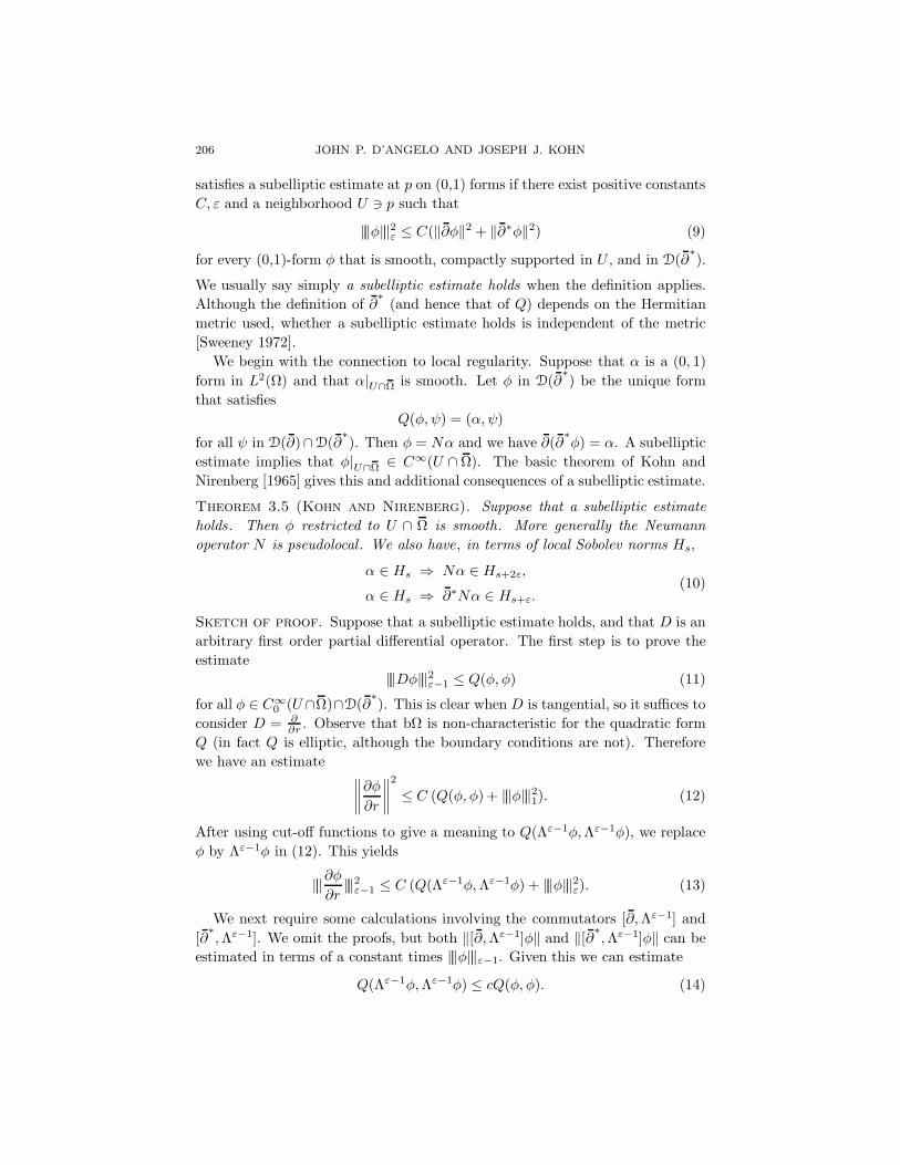
satisfies a subelliptic estimate at p on (0,1) forms if there exist positive constantsC, ε and a neighborhood U 3 p such that
‖‖φ‖‖2ε ≤ C(‖∂φ‖2 + ‖∂∗φ‖2) (9)
for every (0,1)-form φ that is smooth, compactly supported in U , and in D(∂∗).
We usually say simply a subelliptic estimate holds when the definition applies.Although the definition of ∂
∗(and hence that of Q) depends on the Hermitian
metric used, whether a subelliptic estimate holds is independent of the metric[Sweeney 1972].
We begin with the connection to local regularity. Suppose that α is a (0, 1)form in L2(Ω) and that α|U∩Ω is smooth. Let φ in D(∂
∗) be the unique form
that satisfiesQ(φ, ψ) = (α, ψ)
for all ψ in D(∂)∩D(∂∗). Then φ = Nα and we have ∂(∂
∗φ) = α. A subelliptic
estimate implies that φ|U∩Ω ∈ C∞(U ∩ Ω). The basic theorem of Kohn andNirenberg [1965] gives this and additional consequences of a subelliptic estimate.
Theorem 3.5 (Kohn and Nirenberg). Suppose that a subelliptic estimateholds. Then φ restricted to U ∩ Ω is smooth. More generally the Neumannoperator N is pseudolocal . We also have, in terms of local Sobolev norms Hs,
α ∈ Hs ⇒ Nα ∈ Hs+2ε,
α ∈ Hs ⇒ ∂∗Nα ∈ Hs+ε.(10)
Sketch of proof. Suppose that a subelliptic estimate holds, and that D is anarbitrary first order partial differential operator. The first step is to prove theestimate
‖‖Dφ‖‖2ε−1 ≤ Q(φ, φ) (11)
for all φ ∈ C∞0 (U ∩Ω)∩D(∂∗). This is clear when D is tangential, so it suffices to
consider D = ∂∂r . Observe that bΩ is non-characteristic for the quadratic form
Q (in fact Q is elliptic, although the boundary conditions are not). Thereforewe have an estimate ∥∥∥∥∂φ∂r
∥∥∥∥2
≤ C (Q(φ, φ) + ‖‖φ‖‖21). (12)
After using cut-off functions to give a meaning to Q(Λε−1φ,Λε−1φ), we replaceφ by Λε−1φ in (12). This yields
‖‖∂φ∂r‖‖2ε−1 ≤ C (Q(Λε−1φ,Λε−1φ) + ‖‖φ‖‖2ε). (13)
We next require some calculations involving the commutators [∂,Λε−1] and[∂∗,Λε−1]. We omit the proofs, but both ‖[∂,Λε−1]φ‖ and ‖[∂∗,Λε−1]φ‖ can be
estimated in terms of a constant times ‖‖φ‖‖ε−1. Given this we can estimate
Q(Λε−1φ,Λε−1φ) ≤ cQ(φ, φ). (14)
SUBELLIPTIC ESTIMATES AND FINITE TYPE 207
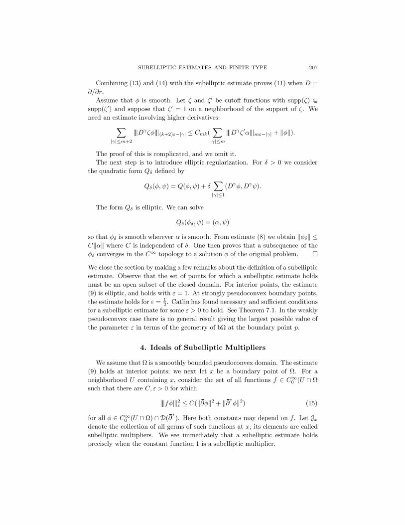
Combining (13) and (14) with the subelliptic estimate proves (11) when D =∂/∂r.
Assume that φ is smooth. Let ζ and ζ′ be cutoff functions with supp(ζ) bsupp(ζ′) and suppose that ζ′ = 1 on a neighborhood of the support of ζ. Weneed an estimate involving higher derivatives:∑
|γ|≤m+2
‖‖Dγζφ‖‖(k+2)ε−|γ| ≤ Cmk(∑|γ|≤m
‖‖Dγζ′α‖‖mε−|γ| + ‖φ‖).
The proof of this is complicated, and we omit it.The next step is to introduce elliptic regularization. For δ > 0 we consider
the quadratic form Qδ defined by
Qδ(φ, ψ) = Q(φ, ψ) + δ∑|γ|≤1
(Dγφ,Dγψ).
The form Qδ is elliptic. We can solve
Qδ(φδ, ψ) = (α, ψ)
so that φδ is smooth wherever α is smooth. From estimate (8) we obtain ‖φδ‖ ≤C‖α‖ where C is independent of δ. One then proves that a subsequence of theφδ converges in the C∞ topology to a solution φ of the original problem.
We close the section by making a few remarks about the definition of a subellipticestimate. Observe that the set of points for which a subelliptic estimate holdsmust be an open subset of the closed domain. For interior points, the estimate(9) is elliptic, and holds with ε = 1. At strongly pseudoconvex boundary points,the estimate holds for ε = 1
2 . Catlin has found necessary and sufficient conditionsfor a subelliptic estimate for some ε > 0 to hold. See Theorem 7.1. In the weaklypseudoconvex case there is no general result giving the largest possible value ofthe parameter ε in terms of the geometry of bΩ at the boundary point p.
4. Ideals of Subelliptic Multipliers
We assume that Ω is a smoothly bounded pseudoconvex domain. The estimate(9) holds at interior points; we next let x be a boundary point of Ω. For aneighborhood U containing x, consider the set of all functions f ∈ C∞0 (U ∩ Ωsuch that there are C, ε > 0 for which
‖‖fφ‖‖2ε ≤ C(‖∂φ‖2 + ‖∂∗φ‖2) (15)
for all φ ∈ C∞0 (U ∩ Ω) ∩D(∂∗). Here both constants may depend on f . Let Jx
denote the collection of all germs of such functions at x; its elements are calledsubelliptic multipliers. We see immediately that a subelliptic estimate holdsprecisely when the constant function 1 is a subelliptic multiplier.
208 JOHN P. D’ANGELO AND JOSEPH J. KOHN
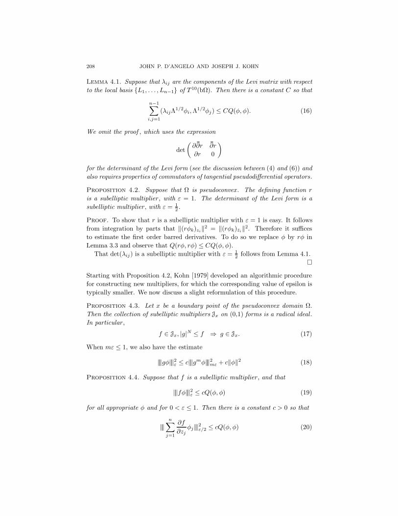
Lemma 4.1. Suppose that λij are the components of the Levi matrix with respectto the local basis L1, . . . , Ln−1 of T 10(bΩ). Then there is a constant C so that
n−1∑i,j=1
(λijΛ1/2φi,Λ1/2φj) ≤ CQ(φ, φ). (16)
We omit the proof , which uses the expression
det(∂∂r ∂r
∂r 0
)for the determinant of the Levi form (see the discussion between (4) and (6)) andalso requires properties of commutators of tangential pseudodifferential operators.
Proposition 4.2. Suppose that Ω is pseudoconvex . The defining function r
is a subelliptic multiplier , with ε = 1. The determinant of the Levi form is asubelliptic multiplier , with ε = 1
2 .
Proof. To show that r is a subelliptic multiplier with ε = 1 is easy. It followsfrom integration by parts that ‖(rφk)zi‖2 = ‖(rφk)zi‖2. Therefore it sufficesto estimate the first order barred derivatives. To do so we replace φ by rφ inLemma 3.3 and observe that Q(rφ, rφ) ≤ CQ(φ, φ).
That det(λij) is a subelliptic multiplier with ε = 12 follows from Lemma 4.1.
Starting with Proposition 4.2, Kohn [1979] developed an algorithmic procedurefor constructing new multipliers, for which the corresponding value of epsilon istypically smaller. We now discuss a slight reformulation of this procedure.
Proposition 4.3. Let x be a boundary point of the pseudoconvex domain Ω.Then the collection of subelliptic multipliers Jx on (0,1) forms is a radical ideal .In particular ,
f ∈ Jx, |g|N ≤ f ⇒ g ∈ Jx. (17)
When mε ≤ 1, we also have the estimate
‖‖gφ‖‖2ε ≤ c‖‖gmφ‖‖2mε + c‖φ‖2 (18)
Proposition 4.4. Suppose that f is a subelliptic multiplier , and that
‖‖fφ‖‖2ε ≤ cQ(φ, φ) (19)
for all appropriate φ and for 0 < ε ≤ 1. Then there is a constant c > 0 so that
‖‖n∑j=1
∂f
∂zjφj‖‖2ε/2 ≤ cQ(φ, φ) (20)

SUBELLIPTIC ESTIMATES AND FINITE TYPE 209
We will use Proposition 4.4 by augmenting the Levi matrix by adding the rows∂f and the column ∂f in the same way we did this for ∂r and ∂r. More precisely,suppose that f1, . . . , fN are subelliptic multipliers. We define the n+ 1 +N byn+ 1 +N matrix A(f) by
A(f) =
∂∂r ∂r ∂f1 . . . ∂fN∂r 0 0 . . . 0∂f1 0 0 . . . 0
......
.... . .
...∂fN 0 0 . . . 0
. (21)
Proposition 4.5. Suppose that fi are subelliptic multipliers. Then the deter-minant of A(f) is a subelliptic multiplier .
Define I0 to be the real radical of the ideal generated by r and the determinantof the Levi form det(λ). For k ≥ 1, define Ik to be the real radical of the idealgenerated by Ik−1 and all determinants det(A(f)) for fj ∈ Ik−1.
By Proposition 4.2 we know that r and det(λ) are subelliptic multipliers. ByProposition 4.3 all the elements in I0 are subelliptic multipliers. By Proposi-tions 4.4 and 4.5, and induction, for each k all the elements of Ik are subellipticmultipliers. Thus a subelliptic estimate holds whenever 1 lies in some Ik.
Definition 4.6. The point p in a pseudoconvex real hypersurface M is of finiteideal-type if there is an integer k such that 1 ∈ Ik. (Equivalently Ik is the ringof germs of smooth functions at p.)
As for the subelliptic estimate, whether p is of finite ideal-type is independentof the Hermitian metric used. Next we prove directly that the existence of acomplex analytic variety V in bΩ prevents points on V from being of finiteideal-type. This theorem motivates Section 6.
Theorem 4.7. Suppose that Ω is pseudoconvex and that there is a complexanalytic variety V lying in bΩ. Then points of V cannot be of finite ideal-type.
Proof. The condition of finite ideal-type is an open condition, so we mayassume that p is a smooth point of V . We may find a non-zero vector field L
that is tangent to V and is a holomorphic combination of the usual Li. Then L isin the kernel of the Levi form along V , so det(λ) vanishes along V . Therefore allelements of I0 vanish on V . We proceed by induction. Suppose that all elementsof Ik−1 vanish along V . Choosing fj ∈ Ik−1 we have L(fj) = 0 because L istangent. Therefore the matrix whose entries are Li(fj) must have a non-trivialkernel, and hence det(A(f)) must vanish on V , and thus all elements of Ik vanishon V also.
For real-analytic pseudoconvex domains, the sequence of ideals stabilizes afterfinitely many steps [Kohn 1979]. Either 1 ∈ Ik for some k, or the processuncovers a real-analytic real subvariety in the boundary of “positive holomorphic
210 JOHN P. D’ANGELO AND JOSEPH J. KOHN
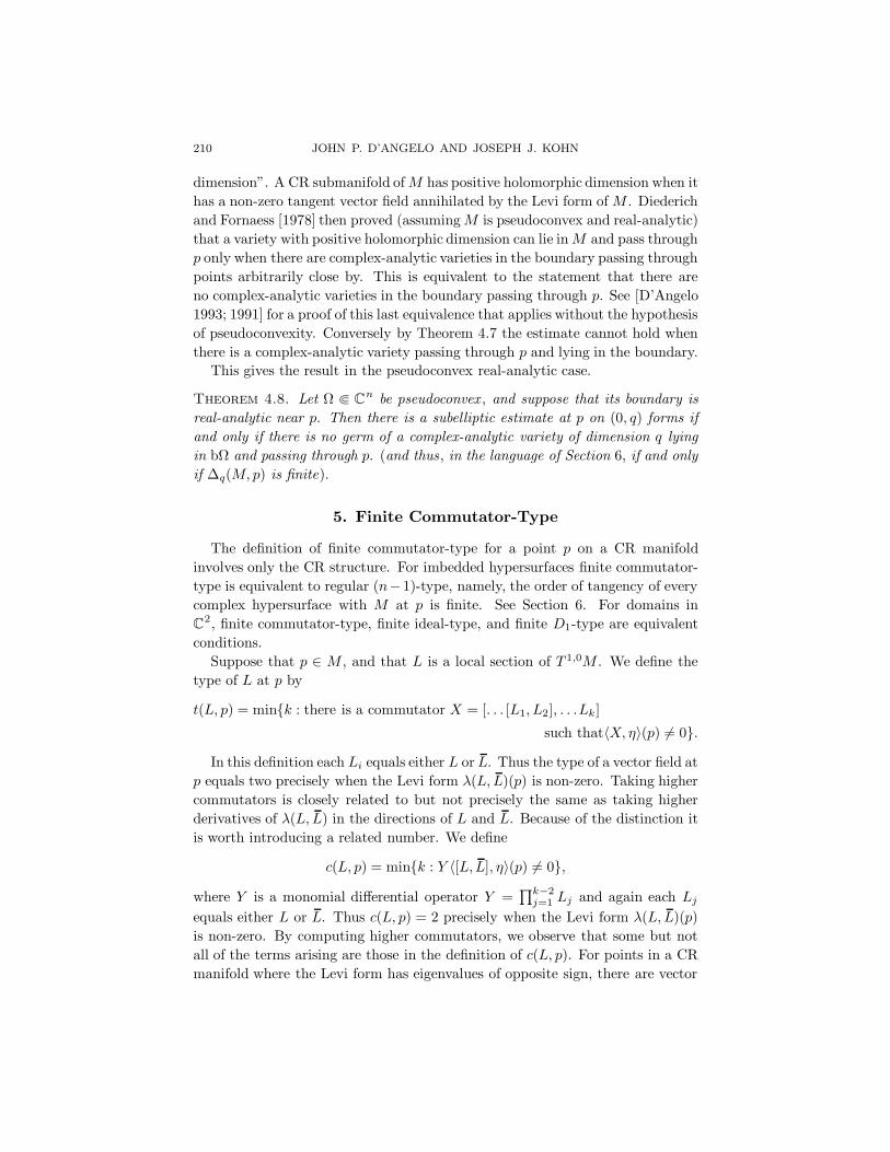
dimension”. A CR submanifold ofM has positive holomorphic dimension when ithas a non-zero tangent vector field annihilated by the Levi form of M . Diederichand Fornaess [1978] then proved (assumingM is pseudoconvex and real-analytic)that a variety with positive holomorphic dimension can lie inM and pass throughp only when there are complex-analytic varieties in the boundary passing throughpoints arbitrarily close by. This is equivalent to the statement that there areno complex-analytic varieties in the boundary passing through p. See [D’Angelo1993; 1991] for a proof of this last equivalence that applies without the hypothesisof pseudoconvexity. Conversely by Theorem 4.7 the estimate cannot hold whenthere is a complex-analytic variety passing through p and lying in the boundary.
This gives the result in the pseudoconvex real-analytic case.
Theorem 4.8. Let Ω b Cn be pseudoconvex , and suppose that its boundary isreal-analytic near p. Then there is a subelliptic estimate at p on (0, q) forms ifand only if there is no germ of a complex-analytic variety of dimension q lyingin bΩ and passing through p. (and thus, in the language of Section 6, if and onlyif ∆q(M, p) is finite).
5. Finite Commutator-Type
The definition of finite commutator-type for a point p on a CR manifoldinvolves only the CR structure. For imbedded hypersurfaces finite commutator-type is equivalent to regular (n−1)-type, namely, the order of tangency of everycomplex hypersurface with M at p is finite. See Section 6. For domains inC2, finite commutator-type, finite ideal-type, and finite D1-type are equivalentconditions.
Suppose that p ∈ M , and that L is a local section of T 1,0M . We define thetype of L at p by
t(L, p) = mink : there is a commutator X = [. . . [L1, L2], . . .Lk]
such that〈X, η〉(p) 6= 0.
In this definition each Li equals either L or L. Thus the type of a vector field atp equals two precisely when the Levi form λ(L, L)(p) is non-zero. Taking highercommutators is closely related to but not precisely the same as taking higherderivatives of λ(L, L) in the directions of L and L. Because of the distinction itis worth introducing a related number. We define
c(L, p) = mink : Y 〈[L,L], η〉(p) 6= 0,
where Y is a monomial differential operator Y =∏k−2j=1 Lj and again each Lj
equals either L or L. Thus c(L, p) = 2 precisely when the Levi form λ(L, L)(p)is non-zero. By computing higher commutators, we observe that some but notall of the terms arising are those in the definition of c(L, p). For points in a CRmanifold where the Levi form has eigenvalues of opposite sign, there are vector

SUBELLIPTIC ESTIMATES AND FINITE TYPE 211
fields for which these numbers are different. It is believed to be true, but notproved in the literature, that these two numbers are the same for all vector fieldsin the pseudoconvex case. See [Bloom 1981; D’Angelo 1993] for what is known.
Next we define the commutator-type of a point on a CR manifold of hyper-surface type.
Definition 5.1. The point p on a CR manifold M of hypersurface type is apoint of finite commutator-type if t(L, p) is finite for some local section L ofT 1,0M . The commutator-type of p is the minimum of the types of all such (1, 0)vector fields L.
We next discuss some geometric aspects of this notion. For a 3-dimensional CRmanifold such as a hypersurface in C2, the space T 1,0
p (M) is 1-dimensional, sothe types of all vector fields non-zero at p are the same. In this case we also havet(L, p) = c(L, p) for all L and p. When the Levi form has n − 2 > 0 positiveeigenvalues and one vanishing eigenvalue on a pseudoconvex CR manifold ofdimension 2n − 1, the minimum value of t(L, p) is two, but furthermore therecan be only one possible value for t(L, p) other than 2 and again t(L, p) =c(L, p) for all L and p. For real hypersurfaces, the commutator-type equals themaximum order of tangency of a complex hypersurface. The geometry becomesmore complicated when the Levi form has several vanishing eigenvalues, and thetypes of vector fields give incomplete information. In particular the conditionthat all (1, 0) vector fields L satisfy t(L, p) < ∞ does not prevent complex-analytic varieties from lying in a hypersurface.
Remark. We discuss the geometric interpretation of the type of a single vectorfield. Suppose that M is a real hypersurface in Cn and that V is a complexmanifold osculating M to order N at p. Then there is a (1, 0) vector field L withL(p) 6= 0 and t(L, p) ≥ N . We may take L to be tangent to V . The converseis not generally true, but the first author believes that it may be true in thepseudoconvex case. We give an example due to Bloom [1981].
Example 5.2. Put r(z, z) = 2 Re(z3) + (z2 + z2 + |z1|2)2, and let M denote thezero set of r. Let p be the origin. Put Lj = ∂/∂zj − rzj ∂/∂z3 for j = 1, 2. In thiscase L1 and L2 form a global basis for sections of T 1,0M . We put L = L1− z1L2.Then λ(L, L)(0) = 0, and the iterated bracket [[L,L], L] vanishes identically.Consequently t(L, p) = ∞. On the other hand, it is easy to check that themaximum order of contact of a complex-analytic curve (whether singular or not)withM at p is 4; in the notation of the next section, ∆Reg
1 (M, p) = ∆1(M, p) = 4.
Singularities create a new difficulty. Suppose that t(L, p) is finite for every localvector field that is non-zero at p. There may nevertheless be a complex varietylying in M and passing through p. Thus the notion of type of a vector field doesnot detect singularities.
Example 5.3. Put r(z, z) = 2 Re(z3)+|f(z1, z2)|2 and let M denote its zero set.Here f is a holomorphic polynomial with f(0, 0) = 0. The complex subvariety
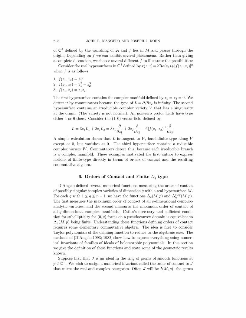
212 JOHN P. D’ANGELO AND JOSEPH J. KOHN
of C3 defined by the vanishing of z3 and f lies in M and passes through theorigin. Depending on f we can exhibit several phenomena. Rather than givinga complete discussion, we choose several different f to illustrate the possibilities:
Consider the real hypersurfaces in C3 defined by r(z, z)=2 Re(z3)+|f(z1, z2)|2when f is as follows:
1. f(z1, z2) = zm12. f(z1, z2) = z2
1 − z32
3. f(z1, z2) = z1z2
The first hypersurface contains the complex manifold defined by z1 = z3 = 0. Wedetect it by commutators because the type of L = ∂/∂z2 is infinity. The secondhypersurface contains an irreducible complex variety V that has a singularityat the origin. (The variety is not normal). All non-zero vector fields have typeeither 4 or 6 there. Consider the (1, 0) vector field defined by
L = 3z1L1 + 2z2L2 = 3z1∂
∂z1+ 2z2
∂
∂z2− 6|f(z1, z2)|2 ∂
∂z3.
A simple calculation shows that L is tangent to V , has infinite type along V
except at 0, but vanishes at 0. The third hypersurface contains a reduciblecomplex variety W . Commutators detect this, because each irreducible branchis a complex manifold. These examples motivated the first author to expressnotions of finite-type directly in terms of orders of contact and the resultingcommutative algebra.
6. Orders of Contact and Finite Dq-type
D’Angelo defined several numerical functions measuring the order of contactof possibly singular complex varieties of dimension q with a real hypersurface M .For each q with 1 ≤ q ≤ n− 1, we have the functions ∆q(M, p) and ∆Reg
q (M, p).The first measures the maximum order of contact of all q-dimensional complex-analytic varieties, and the second measures the maximum order of contact ofall q-dimensional complex manifolds. Catlin’s necessary and sufficient condi-tion for subellipticity for (0, q) forms on a pseudoconvex domain is equivalent to∆q(M, p) being finite. Understanding these functions defining orders of contactrequires some elementary commutative algebra. The idea is first to considerTaylor polynomials of the defining function to reduce to the algebraic case. Themethods of [D’Angelo 1993; 1982] show how to express everything using numer-ical invariants of families of ideals of holomorphic polynomials. In this sectionwe give the definition of these functions and state some of the geometric resultsknown.
Suppose first that J is an ideal in the ring of germs of smooth functions atp ∈ Cn. We wish to assign a numerical invariant called the order of contact to Jthat mixes the real and complex categories. Often J will be I(M, p), the germs

SUBELLIPTIC ESTIMATES AND FINITE TYPE 213
of smooth functions vanishing on a hypersurface M near p. A local definingfunction r for M at p then generates the principal ideal I(M, p).
It is convenient for the definition to write (Ck, x) for the germ of Ck at thepoint x, and to write z : (C, 0) → (Cn, p) when z is the germ of a holomorphicmapping with z(0) = p. To define the order of contact of J with such a z, we pullback the ideal J to one dimension. We write ν(z) = νp(z) for the multiplicity ofz; this is the minimum of the orders of vanishing of the mappings t→ zj(t)−pj .We write ν(z∗r) for the order of vanishing of the function t → r(z(t)) at theorigin. The ratio ∆(J, z) = infr∈J ν(z∗r)/νp(z) is called the order of contact ofJ with the holomorphic curve z. Note that the germ of a curve z is non-singularif ν(z) = 1. The crucial point is that we allow the curves to be singular. For ahypersurface we have the following definition.
Definition 6.1. The order of contact of (the germ at 0 of) a holomorphic curvez with the real hypersurface M at p is the number
∆(M, p, z) = infr∈I(M,p)
ν(z∗r)νp(z)
.
We can compute ∆(M, p, z) by letting r in the definition be a defining function;this gives the infimum.
There are several ways to generalize to singular complex varieties of higherdimension. Below we do this by pulling back to holomorphic curves after wehave restricted to subspaces of the appropriate dimension. Thus we let φ :Cn−q+1 → Cn be a linear embedding, and we consider the subset φ∗M ⊂ Cn−q+1.For generic choices of φ this will be a hypersurface; when it is not we work withideals. We are now prepared to define the numbers ∆q(M, p) and ∆Reg
q (M, p).
Definition 6.2. Let M be a smooth real hypersurface in Cn. For each integerq with 1 ≤ q ≤ n we define ∆q(M, p) and ∆Reg
q (M, p) as follows:
∆1(M, p) = supz
∆(M, p, z),
where the supremum is taken over non-constant germs of holomorphic curves;
∆q(M, p) = infφ
∆1(φ∗M, p),
where the infimum is taken over linear imbeddings φ : Cn−q+1 → Cn; and
∆Reg1 (M, p) = sup
z:ν(z)=1
∆(M, p, z),
where and the supremum is taken over the non-singular germs of holomorphiccurves. The last expression is called the regular order of contact.
For q = 1, . . . , n−1 we take the supremum over all germs z : (Cq, 0)→ (Cn, p)for which dz(0) is injective:
∆Regq (M, p) = sup
zinf
r∈I(M,p)ν(z∗r)

214 JOHN P. D’ANGELO AND JOSEPH J. KOHN
We also put ∆n(M, p) = ∆Regn (M, p) = 1 for convenience.
Example 6.3. Put r(z, z) = Re(z4) + |z1z2− z53 |2, and let p be the origin. Note
that the image of the map (s, t)→ (s5, t5, st, 0) lies in M , but that its derivativeis not injective at 0. This shows that ∆2(M, p) = ∞. On the other hand∆Reg
2 (M, 0) = 10; the map (s, t) → (s, 0, t, 0) for example gives the supremum.We have
(∆4(M, 0),∆3(M, 0),∆2(M, 0),∆1(M, 0)) = (1, 4,∞,∞),
(∆Reg4 (M, 0),∆Reg
3 (M, 0),∆Reg2 (M, 0),∆Reg
1 (M, 0)) = (1, 4, 10,∞).
Definition 6.4. Let M be a smooth real hypersurface in Cn. The pointp ∈M is of finite Dq- type if ∆q(M, p) is finite. It is of finite regular Dq-type is∆Regq (M, p) is finite.
One of the main geometric results is local boundedness for the function p →∆q(M, p). This shows that finite Dq-type is an open non-degeneracy condition.The condition is also finitely determined. See [D’Angelo 1993] for a completediscussion of these functions.
Theorem 6.5. Let M be a smooth real hypersurface in Cn. The functionp→ ∆q(M, p) is locally bounded ; if p is near po then
∆q(M, p) ≤ 2(∆q(M, po))n−q
Suppose additionally that M is pseudoconvex . For each q with 1 ≤ q ≤ n− 1 thefunction p→ ∆q(M, p) satisfies the following sharp bounds: if p is near po then
∆q(M, p) ≤ ∆q(M, po)n−q/2n−1−q.
Corollary. For each q ≥ 1, the set of points of finite Dq-type is an open subsetof M .
The set of points of finite regular Dq-type is not generally open when q < n− 1.See Example 5.3.2.
We remark also on additional information available in the real-analytic case[D’Angelo 1993; 1991; Diederich and Fornaess 1978] and sharper informationin the algebraic case (when there is a polynomial defining equation) [D’Angelo1983].
Theorem 6.6. Let M be a real-analytic real hypersurface in Cn. Then either∆1(M, p) is finite or there is a 1-dimensional complex-analytic variety containedin M and passing through p. If M is compact , then the first alternative musthold .
When the defining equation is a polynomial there is quantitative informationdepending only on the dimension and the degree of the polynomial [D’Angelo1983].

SUBELLIPTIC ESTIMATES AND FINITE TYPE 215
Theorem 6.7. Let M be a real hypersurface in Cn defined by a polynomialequation of degree d. Then either ∆1(M, p) ≤ 2d(d−1)n−1 or there is a complex-analytic 1-dimensional variety contained in M and passing through p. Further-more, there is an explicit way to find the defining equations of the complex varietydirectly from the defining equation for M .
Theorems 6.5 and 6.7 rely upon writing real-valued polynomials as differencesof squared norms of holomorphic mappings; it is easy to decide when the zerosets of such expressions contain complex analytic varieties. The method enablesone to work in the category of holomorphic polynomials and to use elementarycommutative algebra.
We mention briefly what this entails. We consider the ring of germs of holo-morphic functions at a point and its maximal ideal M. Saying that a properideal I of germs of holomorphic functions is primary to the maximal ideal M isequivalent to saying that its elements vanish simultaneously only at the origin(Nullstellensatz). It is then possible to assign numerical invariants that mea-sure the singularity defined by the primary ideal, such as the order of contact,the smallest power of M contained in I, the codimension of I, etc. Inequali-ties among these invariants are crucial to the proofs of Theorems 6.5 and 6.7.Consider again the domains defined by (2); the origin is of finite D1-type if andonly if the ideal (f1, . . . fN , zn) is primary to M. One sees that the passage fromstrongly pseudoconvex points to points of finite D1-type precisely parallels thepassage from the maximal ideal M to ideals primary to it.
7. Catlin’s Multitype and Sufficient Conditions for SubellipticEstimates
Catlin generalized Theorem 4.8 to the smooth case. In [Catlin 1983; 1984;1987] he established that finite type is a necessary and sufficient condition forsubellipticity on pseudoconvex domains. In most of this section we consider theresults for (0, 1) forms.
Theorem 7.1. Let Ω b Cn be a pseudoconvex domain with smooth boundary.Then there is a subelliptic estimate at p if and only if ∆1(bΩ, p) < ∞. Theparameter epsilon from Definition 3.4 must satisfy ε ≤ 1
∆1(bΩ,p).
We start by discussing the proof that finite type implies that subelliptic estimateshold. Catlin applies the method of weight functions used earlier by Hormander[1966]. Rather than working with respect to Lebesgue measure dV , consider themeasure e−Φ dV where Φ will be chosen according to the needs of the problem.After this choice is properly made, one employs, as a substitute for Lemma 3.3,the inequality ∫
Ω
n∑i,j=1
Φzizjaiaj dV +n∑
j,k=1
‖Ljak‖2 ≤ CQ(a, a), (22)
216 JOHN P. D’ANGELO AND JOSEPH J. KOHN
where |Φ| ≤ 1. Here Lj are (0, 1) vector fields on Cn. There could be also a termon the left side involving the boundary integral of the Levi form, but such a termdoes not need to be used in this approach to the estimates. Instead, one needsto choose Φ with a large Hessian. One step in Catlin’s proof is the followingreduction:
Theorem 7.2. Suppose that Ω b Cn is a pseudoconvex domain defined byΩ = r < 0, and that p ∈ bΩ. Let U be a neighborhood of p. Suppose that forall δ > 0 there is a smooth real-valued function Φδ satisfying the properties:
|Φδ| ≤ 1 on U,
(Φδ)zizj ≥ 0 on U,n∑
i,j=1
(Φδ)zizjaiaj ≥ c|a|2δ2ε
on U ∩ −δ < r ≤ 0. (23)
Then there is a subelliptic estimate of order ε at p.
Theorem 7.2 reduces the problem to constructing such bounded smooth plurisub-harmonic functions whose Hessians are at least as large as δ−2ε. One of the cru-cial ingredients is the use of an n-tuple of rational numbers (+∞ is also allowed)called the multitype. This n-tuple differs from both the n-tuples of orders ofcontact or of regular orders of contact. There are inequalities in one direction; insimple geometric situations there may be equality. Later we mention the workof Yu in this direction.
We give some motivation for the use of the multitype. Suppose that W ⊂Mis a manifold of holomorphic dimension zero. Recall that W is a CR submanifoldof M , and that the Levi form for M does not annihilate any (1, 0) vector fieldstangent to W . It follows from the discussion in Section 3 that the distance dWis a subelliptic multiplier. Suppose that we have a subelliptic estimate awayfrom W . We then obtain a subelliptic estimate (with a smaller epsilon) on W
as well, because dW is a subelliptic multiplier. Hence manifolds of holomorphicdimension zero are small sets as far as the estimates are concerned. This suggestsa stratification of M .
Suppose now that p is a point of finite Dq-type, and that U is a neighborhoodof p in bΩ where ∆q(M, p) ≤ 2(∆q(M, po))n−q . Catlin defines the multitype asan n-tuple of rational numbers, and shows that it assumes only finitely manyvalues in U . The stratification is then given by the level sets of the multitypefunction. Catlin proves that each such level set is locally contained in a manifoldof holomorphic dimension at most q − 1. Establishing the properties of themultitype is difficult, and involves showing that the multitype equals another n-tuple called the commutator type. The commutator type generalizes the notionsof Section 3. See [Catlin 1984] for this material.
We next define the multitype. Let µ = (µ1, . . . , µn) be an n-tuple of numbers(or plus infinity) with 1 ≤ µj ≤ ∞ and such that µ1 ≤ µ2 ≤ . . . ≤ µn. We
SUBELLIPTIC ESTIMATES AND FINITE TYPE 217
demand that, whenever µk is finite, we can find integers nj so that
k∑j=1
njµj
= 1.
We call such n-tuples weights, and order them lexicographically. Thus, for exam-ple, (1, 2,∞) is considered smaller than (1, 4, 6). A weight is called distinguishedif we can find local coordinates so that p is the origin and such that
n∑j=1
aj + bjµj
< 1 ⇒ DaDbr(0) = 0, (24)
where a = (a1, . . . , an) and b = (b1, . . . , bn) are multi-indices. The multitypem(p) is the smallest weight that dominates (in the lexicographical ordering)every distinguished weight µ. In some sense we are assigning weights mj tothe coordinate direction zj and measuring orders of vanishing. The followingstatements are automatic from the definition. If the Levi form has rank q − 1at p, then mj(p) = 2 for 2 ≤ j ≤ q. In general m1(p) = 1, and m2(p) =∆n−1(M, p) = ∆Reg
n−1(M, p).
Example 7.3. Let M be the hypersurface in C3 defined by
r(z, z) = 2 Re(z3) + |z21 − z3
2 |2.
The multitype at the origin is (1, 4, 6) and (∆3(M, 0),∆2(M, 0),∆1(M, 0)) =(1, 4,∞). Thus a finite multitype at p does not guarantee that p is of finiteD1-type. At points of the form (t3, t2, 0) for a non-zero complex number t,the multitype will be (1, 2,∞). This illustrates the upper semicontinuity of themultitype in the lexicographical sense, because (1, 2,∞) is smaller than (1, 4, 6).
Catlin proved that the multitype on a pseudoconvex hypersurface is upper semi-continuous in this lexicographical sense. He also proved the collection of inequal-ities given, for 1 ≤ q ≤ n, by
mn+1−q(p) ≤ ∆q(M, p). (25)
Yu [1994] defined a point to be h-extendible if equality in (25) holds for eachq. This class of boundary points exhibits simpler geometry than the generalcase. Yu proved that convex domains of finite D1-type are h-extendible, afterMcNeal [1992] had proved for convex domains with boundaryM that ∆1(M, p) =∆Reg
1 (M, p). Yu then gave a nice application, that h-extendible boundary pointsmust be peak points for the algebra of functions holomorphic on the domainand continuous up to the boundary. McNeal applied his result to the boundarybehavior of the Bergman kernel function on convex domains.
Sibony has studied the existence of strongly plurisubharmonic functions withlarge Hessians as in Theorem 7.2. He introduced the notion that a compact

218 JOHN P. D’ANGELO AND JOSEPH J. KOHN
subset X ⊂ Cn be B-regular. The intuitive idea is that such a subset is B-regular when it contains no analytic structure in a certain strong sense. Sibonyhas given several equivalent formulations of this notion; one is that the algebra ofcontinuous functions on X is the same as the closure of the algebra of continuousplurisubharmonic functions defined near the set. Another equivalence is theexistence, given a real number s, of a plurisubharmonic function, defined nearX and bounded by unity, whose Hessian has minimum eigenvalue at least severywhere on X. Catlin proved for example that a submanifold of holomorphicdimension 0 in a pseudoconvex hypersurface is necessarily B-regular. See [Sibony1991] for considerable discussion of B-regularity and additional applications.
8. Necessary Conditions and Sharp Subelliptic Estimates
We next discuss necessity results for subelliptic estimates. Greiner [1974]proved that finite commutator-type is necessary for subelliptic estimates in twodimensions. Rothschild and Stein [1976] proved in two dimensions that thelargest possible value for ε is the reciprocal of t(L, p), where L is any (1, 0) vectorfield that doesn’t vanish at p. In higher dimensions finite commutator-type doesnot guarantee a subelliptic estimate on (0, 1) forms. Furthermore, Example 5.3.2shows that t(L, p) can be finite for every (1, 0) vector field L while subellipticestimates fail.
Although finite D1-type is necessary and sufficient, an example of D’Angeloshows that one cannot in general choose epsilon as large as the reciprocal ofthe order of contact [D’Angelo 1982; 1980]. The result is very simple. Thefunction p→ ∆1(bΩ, p) is not in general upper semicontinuous, so its reciprocalis not lower semicontinuous. Definition 3.4 reveals that, if there is a subellipticestimate of order epsilon at one point, then there also is one at nearby points.Catlin has shown that the parameter value cannot be determined by informationbased at one point alone [Catlin 1983]. Nevertheless Theorem 6.5 shows that thecondition of finite type does propagate to nearby points. This suggests that onecan always choose epsilon as large as ε = 2n−2/(∆1(bΩ, p))n−1. A more preciseconjecture is that we may always choose epsilon as large as ε = 1/B(bΩ, p). Thedenominator is the “multiplicity” of the point, defined in [D’Angelo 1993], whereit is proved that the function p→ B(M, p) is upper semicontinuous.
Determining the precise largest value for ε seems to be difficult. See Exam-ple 8.1 and Proposition 8.3 below. An example from [D’Angelo 1995] considersdomains of the form (2), where for j = 1, . . . , n−1 the functions fj are arbitraryWeierstrass polynomials of degree mj in zj that depend only on (z1, . . . , zj). Themultiplicity in this case is B(bΩ, p) = 2
∏mj . It is possible, using the method of
subelliptic multipliers, to obtain a value of epsilon that works uniformly over allsuch choices of Weierstrass polynomials and depends only upon these exponents.The result is much smaller than the reciprocal of the multiplicity.
SUBELLIPTIC ESTIMATES AND FINITE TYPE 219
We next illustrate the difficulty in obtaining sharp subelliptic estimates. Theexistence of the estimate at a point can be decided by examining a finite Taylorpolynomial of the defining function there, because finite D1-type is a finitelydetermined condition. This Taylor polynomial does not determine the sharpvalue of epsilon. Suppose that l, m are integers with m ≥ l ≥ 2.
Example 8.1. Consider the pseudoconvex domain, defined near the origin, bythe function r, where
r(z, z) = 2 Re(z3) + |z21 − z2z
l3|2 + |z2|4 + |z1z
m3 |2.
We have ∆1(bΩ, 0) = 4 and B(bΩ, 0) = 8. Catlin [1983] proved that the largestε for which there is a subelliptic estimate in a neighborhood of the origin equalsm+2l
4(2m+l) . This number takes on values between 14 (when m = l) and 1
8 . Thisinformation supports the conjecture that the value of the largest ε satisfies
1B(bΩ, 0)
≤ ε ≤ 1∆1(bΩ, 0)
.
In order to avoid singularities and obtain precise results, Catlin [1983] considersfamilies of complex manifolds. Suppose that T is a collection of positive numberswhose limit is 0. For each t ∈ T we consider a biholomorphic image Mt = gt(Bt)of the ball of radius t about 0 in Cq. We suppose that the derivatives dgt satisfyappropriate uniformity conditions. In particular we need certain q by q minordeterminants of dgt to be uniformly bounded away from 0. We may then pullback r to gt and define the phrase “The order of contact of the family Mt withbΩ at the origin is at least η” by decreeing that sup |g∗t r| ≤ Ctη.
Catlin proved the following precise necessity result.
Theorem 8.2. Suppose that bΩ is smooth and pseudoconvex and that there isa family Mt of q-dimensional complex manifolds whose order of contact with bΩat a boundary point p is at least η. If there is a subelliptic estimate at p on (0, q)forms for some ε, then ε ≤ 1
η .
Catlin has also proved the following unpublished result.
Proposition 8.3. Suppose that ε is a real number with 0 < ε ≤ 14. Then there
is a smooth pseudoconvex domain in C3 such that a subelliptic estimate holdswith parameter ε but for no larger number . If ε is a rational number in thisinterval , then there is a pseudoconvex domain in C3 with a polynomial definingequation such that a subelliptic estimate holds with parameter ε but for no largernumber .
Sketch of proof. Consider the pseudoconvex domain Ω defined by the fol-lowing generalization of Example 8.1. We suppose that f, g are holomorphicfunctions, vanishing at the origin, and satisfying |g(z)| ≤ |f(z)|. We put
r(z, z) = 2 Re(z3) + |zm1 − z2f(z3)|2 + |z2|2m + |g(z3)z2|2.
220 JOHN P. D’ANGELO AND JOSEPH J. KOHN
It is easy to see that ∆1(bΩ, p) = 2m and that B(bΩ, p) = 2m2 no matter whatthe choices of f, g are. It is possible to explicitly compute the largest possiblevalue of the parameter ε in many cases. By putting f(z3) = zp3 and g(z3) = zq3 onecan show that ε = (q+ p(m− 1))/(2m2q), exhibiting the entire range of rationalnumbers between the reciprocals of the the D1-type 2m and the multiplicity 2m2.To see that ε is at most this number one considers the family of complex one-dimensional manifoldsMt defined by the parametric curves ζ → (ζ, ζm/(it)p, it)for ζ ∈ C satisfying |ζ| ≤ |t|α for some exponent α. By choosing α appropriatelyone can compute the contact of this family of complex manifolds, and obtainε ≤ (q + p(m − 1))/(2m2q). To show that equality holds one must constructexplicitly the functions needed in Theorem 7.2. More complicated choices of f, genable us to obtain any real number in this range.
Remark. Catlin has made other choices of f, g in the examples from Proposi-tion 8.3 to draw a remarkable conclusion. For any η with 0 < η ≤ 1
4 , there is asmoothly bounded pseudoconvex domain in C3 such that a subelliptic estimateholds for all ε less than η, but not for η.
9. Domains in Manifolds
Suppose now that X is a complex manifold with Hermitian metric gij. LetΩ be a pseudoconvex domain in X with compact closure and smooth boundary.We still have the notions of defining function, vector fields and forms of type(1,0) as before. We have |∂r|2 =
∑gijrzirzj in a local coordinate system. In
a small neighborhood U of a point p ∈ bΩ we suppose that ω1, . . .ωn form anorthonormal basis for the (1,0) forms. We may suppose that ωn = (∂r)/|∂r|.Let Li be a basis of (1,0) vector fields dual to ωj in U . We can write a(0,1)-form φ as φ =
∑φiωi. When u is a function we have ∂u =
∑Li(u)wi.
Applying ∂ to φ we have
∂φ =∑i<j
Li(φj)wi ∧wi +∑
φi∂ωi.
Suppose now that φ is supported in U , and that φ ∈ D(∂∗). We can write
(∂∗φ, u) =
∑Li∗φi, u+
∑∫bΩ
Li(r)φiu dS. (26)
We have Li(r) = 0 unless i = n. From (26) we see that the boundary conditionis given by φn = 0, and that
∂∗φ = −
∑Liφi +
∑aiφi
for smooth functions ai.

SUBELLIPTIC ESTIMATES AND FINITE TYPE 221
Following the proof of Lemma 3.3, and absorbing terms appropriately weobtain the basic estimate. Note that we require ‖φ‖2 on the right hand side:
∑i,j
‖Liφj‖2 +n∑
i,j=1
∫bΩ
λijφiφjdS ≤ C(Q(φ, φ) + ‖φ‖2)
Recall our earlier remark that, when X = Cn, we can estimate ‖φ‖2 ≤CQ(φ, φ). This implies that the space of harmonic (0,1) forms H0,1 consistsof 0 alone. For a general Hermitian manifold X, this will not be true.
The definition of the tangential Sobolev norms in the manifold setting usespartitions of unity. Assuming this definition, suppose that Ω is a domain in aHermitian complex manifold X. We say that the ∂-Neumann problem satisfiesa subelliptic estimate at p ∈ bΩ if, for a sufficiently small neighborhood U of p,there are positive constants C, ε so that
‖‖φ‖‖2ε ≤ C(‖∂φ‖2 + ‖∂∗φ‖2) (27)
for every (0,1)-form φ that is smooth, compactly supported in U , and in D(∂).Note that (8) holds for φ supported in sufficiently small neighborhoods, so wedo not require putting ‖φ‖2 on the right side of (27).
Suppose that φν is a bounded sequence in the ‖‖φ‖‖ε norm. Then there isa convergent subsequence in L2. In other words, the inclusion mapping is acompact operator. Hence the harmonic space H0,1 is finite-dimensional. Fur-thermore harmonic forms are smooth on Ω. Finally we have the usual Hodgedecomposition. See [Kohn and Nirenberg 1965] for the details.
10. Domains That Are Not Pseudoconvex
Suppose now that Ω is a domain in Cn with smooth but not pseudoconvexboundary. Let λ denote the Levi form, considered at each boundary point p asa linear transformation from T 10
p (M) to itself. We write Tr(λ) for the trace ofthis linear mapping. (Since the Levi form is defined up to a multiple, the trace isalso defined up to a multiple.) We write Id for the identity operator on T 10
p (M).For a point p ∈ bΩ, we consider two possible positivity conditions.
Condition 1 (Pseudoconvexity). There is a neighborhood of p on which λ ≥ 0.Condition 2. There is a neighborhood of p on which λ ≥ Tr(λ) Id.
In case 1 holds we have already defined finite ideal-type and seen that finiteideal-type implies that a subelliptic estimate holds. We now define ideals ofsubelliptic multipliers in case condition 2 holds. (See [Kohn 1985]).
We let J0 be the real radical of the ideal generated by a defining functionr and by the determinant of the mapping λ − Tr(λ) Id. Given a collection offunctions f = f1, . . . , fN we define a linear transformation B(f) on T 10(M) and

222 JOHN P. D’ANGELO AND JOSEPH J. KOHN
corresponding Hermitian form by
〈B(f)ζ, ζ〉 = 〈(λ−Tr(λ) Id)ζ, ζ〉+N∑j=1
(|∂bfj ⊗ ζ|2 − |〈∂bfj, ζ〉|2).
In coordinates we have∑m,l
Bml(f)ζmζ l =∑i,j
λijζiζj − Tr(λ)∑i
|ζi|2 +∑i,j,k
|Lj(fk)ζi − Li(fk)ζj |2.
When condition 2 holds we define the ideals Jk inductively. We let Jk be thereal radical of the ideal generated by Jk−1 and the determinants of all matricesB(f) for fj ∈ Jk−1. When condition 2 holds we say that p is of finite ideal-typeif there is an integer k for which 1 ∈ Jk, that is, the ideal Jk is the full ring ofgerms of smooth functions at p.
Proposition 10.1. Suppose that condition 2 holds, and that p is of finite ideal-type. Then there is a subelliptic estimate in the ∂-Neumann problem on (0, 1)forms.
Proof. We begin with some lemmas.
Lemma 10.2. Suppose that i, j are less than n. Then
‖Li(φj)‖2 = ‖Li(φj)‖2−∫
bΩ
λii|φj|2dS+0(‖φj‖∑k<n
‖Lkφj‖+‖Lnφj‖2)+‖φj‖2)
(28)
Sketch of proof. Begin with ‖Li(φj)‖2 = (Li(φj), Li(φj)) and integrate byparts twice using Stokes’s theorem. At one point write LiLi = LiLi − [Li, Li].Then note that the T component of [Li, Li] equals λii, and integrate the termcontaining this by parts again to get a boundary integral of λii|φj|2. The otherterms get estimated by the Schwartz inequality.
Lemma 10.3. There is a positive constant C such that , for smooth φ ∈ D(∂∗),∑
i,j<n
‖Li(φj)‖2 +∑j
‖Lnφj‖2 +n∑
i,j=1
∫bΩ
λijφiφj dS
−∫
bΩ
Tr(λ)|φ|2 dS ≤ C(Q(φ, φ) + ‖φ‖2).
Proof. Take the sum over i, j in (28) and substitute in the basic estimate.Estimate the other terms by the small constant large constant trick.
To finish the proof of Proposition 10.1, we suppose that f is a subelliptic multi-plier, so that ‖‖fφ‖‖2ε ≤ CQ(φ, φ). Next we verify that∑
i,j<n
‖‖Li(f)φj − Lj(f)φi‖‖2ε2≤ CQ(φ, φ).
SUBELLIPTIC ESTIMATES AND FINITE TYPE 223
This inequality is dual to the estimate of Proposition 4.4. Suppose that f is asubelliptic multiplier. Given any Hermitian form W (φ, φ) whose determinant isa subelliptic multiplier, we form a new form W ′ defined by
W ′(φ, φ) = W (φ, φ) +∑i,j<n
‖Li(f)φj − Lj(f)φi‖2.
As before we see that the determinant of the coefficient matrix of W ′ is also asubelliptic multiplier.
Proposition 10.1 follows by iterating this operation.
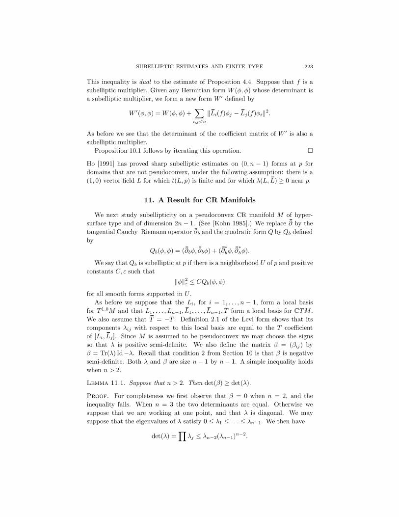
Ho [1991] has proved sharp subelliptic estimates on (0, n − 1) forms at p fordomains that are not pseudoconvex, under the following assumption: there is a(1, 0) vector field L for which t(L, p) is finite and for which λ(L, L) ≥ 0 near p.
11. A Result for CR Manifolds
We next study subellipticity on a pseudoconvex CR manifold M of hyper-surface type and of dimension 2n − 1. (See [Kohn 1985].) We replace ∂ by thetangential Cauchy–Riemann operator ∂b and the quadratic form Q by Qb definedby
Qb(φ, φ) = (∂bφ, ∂bφ) + (∂∗bφ, ∂
∗bφ).
We say that Qb is subelliptic at p if there is a neighborhood U of p and positiveconstants C, ε such that
‖φ‖2ε ≤ CQb(φ, φ)
for all smooth forms supported in U .As before we suppose that the Li, for i = 1, . . . , n − 1, form a local basis
for T 1,0M and that L1, . . . , Ln−1, L1, . . . , Ln−1, T form a local basis for CTM .We also assume that T = −T . Definition 2.1 of the Levi form shows that itscomponents λij with respect to this local basis are equal to the T coefficientof [Li, Lj]. Since M is assumed to be pseudoconvex we may choose the signsso that λ is positive semi-definite. We also define the matrix β = (βij) byβ = Tr(λ) Id−λ. Recall that condition 2 from Section 10 is that β is negativesemi-definite. Both λ and β are size n − 1 by n− 1. A simple inequality holdswhen n > 2.
Lemma 11.1. Suppose that n > 2. Then det(β) ≥ det(λ).
Proof. For completeness we first observe that β = 0 when n = 2, and theinequality fails. When n = 3 the two determinants are equal. Otherwise wesuppose that we are working at one point, and that λ is diagonal. We maysuppose that the eigenvalues of λ satisfy 0 ≤ λ1 ≤ . . . ≤ λn−1. We then have
det(λ) =∏
λj ≤ λn−2(λn−1)n−2.

224 JOHN P. D’ANGELO AND JOSEPH J. KOHN
We have βj = Tr(λ) − λj =∑k 6=j λk. Since all the λj are non-negative, we
can drop terms and easily obtain
det(β) =∏
βj ≥ λn−2(λn−1)n−2,
and the result follows.
Proceeding as in Section 10 we obtain the two basic estimates∑‖Liφj‖2 +
∑(λijTφi, φj) ≤ Qb(φ, φ) + 0(‖φ‖2 + ‖φ‖
∑‖Lkφj‖),∑
‖Liφj‖2 −∑
(βijTφi, φj) ≤ Qb(φ, φ) + 0(‖φ‖2 + ‖φ‖∑‖Lkφj‖).
Proposition 11.2. Suppose that n > 2. Let λ = (λij) be the Levi matrix withrespect to the local basis L1, . . . , Ln−1 of T 1,0(M). Then there is a constant Cso that , for all smooth φ supported in U ,
(det(λ)Λ1/2φ,Λ1/2φ) ≤ CQb(φ, φ).
Proof. We need to microlocalize the two basic estimates. We suppose that weare working in a coordinate neighborhood U of a point p, where our coordinatesare denoted by x1, . . . , x2n−2, t. We may assume that these coordinates havebeen chosen so that, at p, we have T = (1/
√−1)(∂/∂t) and Lj = 1
2 (∂/∂x2j−1−√−1 ∂/∂x2j).Let ξ1, . . . , ξ2n−2, τ denote the dual coordinates in the Fourier transform space.
We may also assume that T = (1/√−1)∂/∂t in the full neighborhood.
Suppose that u is smooth and supported in U . Write
u = u+ + u− + u0,
where u+ is supported in a conical neighborhood of 0 with τ > 0, u− is supportedin a conical neighborhood of 0 with τ < 0, and u0 is supported outside of suchneighborhoods.
Since Qb is elliptic on the support of u0, we have the estimate
‖ det(λ)φ0‖212≤ C‖φ0‖21 ≤ CQb(φ, φ)
By Garding’s inequality we have the estimates
(det(λ)Tφ+, φ+) ≥ −c‖φ‖2, (det(β)Tφ−, φ−) ≥ −c‖φ‖2.
We also have
(det(λ)Tφ+, φ+) = (det(λ)Λ1/2φ+,Λ1/2φ+) + · · · ,(det(β)Tφ−, φ−) = (det(β)Λ1/2φ−,Λ1/2φ−) + · · · ,
Here the dots denote error terms. Using the basic estimates we obtain
n−1∑i,j=1
(λijΛ1/2φ+i ,Λ
1/2φ+j ) ≤ CQb(φ, φ)
SUBELLIPTIC ESTIMATES AND FINITE TYPE 225
andn−1∑i,j=1
(bijΛ1/2φ−i ,Λ1/2φ−j ) ≤ CQb(φ, φ).
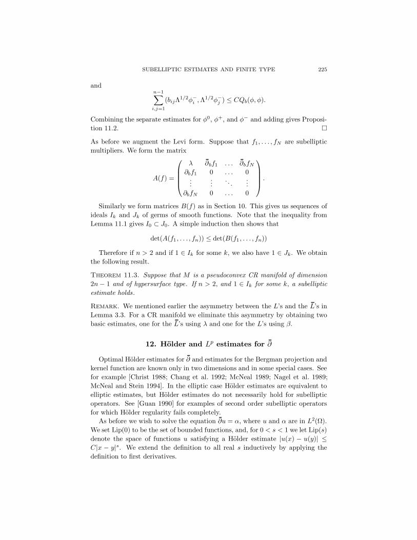
Combining the separate estimates for φ0, φ+, and φ− and adding gives Proposi-tion 11.2.
As before we augment the Levi form. Suppose that f1, . . . , fN are subellipticmultipliers. We form the matrix
A(f) =
λ ∂bf1 . . . ∂bfN∂bf1 0 . . . 0
......
. . ....
∂bfN 0 . . . 0
.
Similarly we form matrices B(f) as in Section 10. This gives us sequences ofideals Ik and Jk of germs of smooth functions. Note that the inequality fromLemma 11.1 gives I0 ⊂ J0. A simple induction then shows that
det(A(f1, . . . , fn)) ≤ det(B(f1, . . . , fn))
Therefore if n > 2 and if 1 ∈ Ik for some k, we also have 1 ∈ Jk. We obtainthe following result.
Theorem 11.3. Suppose that M is a pseudoconvex CR manifold of dimension2n− 1 and of hypersurface type. If n > 2, and 1 ∈ Ik for some k, a subellipticestimate holds.
Remark. We mentioned earlier the asymmetry between the L’s and the L’s inLemma 3.3. For a CR manifold we eliminate this asymmetry by obtaining twobasic estimates, one for the L’s using λ and one for the L’s using β.
12. Holder and Lp estimates for ∂
Optimal Holder estimates for ∂ and estimates for the Bergman projection andkernel function are known only in two dimensions and in some special cases. Seefor example [Christ 1988; Chang et al. 1992; McNeal 1989; Nagel et al. 1989;McNeal and Stein 1994]. In the elliptic case Holder estimates are equivalent toelliptic estimates, but Holder estimates do not necessarily hold for subellipticoperators. See [Guan 1990] for examples of second order subelliptic operatorsfor which Holder regularity fails completely.
As before we wish to solve the equation ∂u = α, where u and α are in L2(Ω).We set Lip(0) to be the set of bounded functions, and, for 0 < s < 1 we let Lip(s)denote the space of functions u satisfying a Holder estimate |u(x) − u(y)| ≤C|x − y|s. We extend the definition to all real s inductively by applying thedefinition to first derivatives.

226 JOHN P. D’ANGELO AND JOSEPH J. KOHN
Let p be a boundary point of commutator-type m. Suppose that ζα ∈ Lip(s)for all smooth cut-off functions ζ for some s. Let u denote the ∂-Neumannsolution to ∂u = α, so u is orthogonal to the holomorphic functions. Feffermanand Kohn showed that ζu ∈ Lip(s + 1
m) for all smooth cut-off functions ζ.This result requires that s + 1
m not be an integer, although they obtain thecorresponding result in that case as well, by giving a different definition of theLipschitz spaces for integer values of s. Write LIP(s) for this class of spaces; fors not an integer Lip(s) = LIP(s). They proved also that both the Bergman andSzego projection preserve Lipschitz spaces.
For bounded pseudoconvex domains in Cn the range of ∂b in L2 is closed; see[Kohn 1986; Shaw 1985]. For general CR manifolds (even in the strongly pseudo-convex 3-dimensional case) it is required to assume this. Given the assumptionof closed range, all these results follow from the analysis of a second-order pseu-dodifferential operator A on R3. Fefferman and Kohn [1988] prove that solutionsu They prove that solutions u to the equation Au = f lie in LIP(s + 2
m) when
f ∈ LIP(s) near a point of commutator-type m. See [Fefferman 1995] for adiscussion of the operator A and the techniques of microlocal analysis needed.The techniques also work [Fefferman et al. 1990] in the restricted case in higherdimensions where the Levi form is smoothly diagonalizable.
There are many special cases where estimates for the Bergman and Szegoprojections and Lp estimates for ∂ have been proved by other methods. Fornaessand Sibony [1991] construct a smoothly bounded pseudoconvex domain suchthat, for certain α ∈ Lp with p > 2, the equation ∂u = α has no solution inLp′
for all p′ in a certain range of values ≤ p. They also prove a positive resultfor Runge domains. Chang, Nagel and Stein [Chang et al. 1992] give preciseestimates in various function spaces for solutions of ∂u = α on domains of finitecommutator-type in C2. See [McNeal and Stein 1994] for estimates (Sobolev,Lipschitz, anisotropic Lipschitz) on convex domains of finite type in arbitrarydimensions. We do not discuss these results here.
13. Brief Discussion of Related Topics
Many different finite-type conditions arise in complex analysis. Here we brieflydescribe some situations where precise theorems are known in various finite-typesettings. The reader should consult the bibliographies in the papers we mentionfor a complete overview.
Hans Lewy [1956] first studied the extension of CR functions from a stronglypseudoconvex real hypersurface. After work by many authors, usually involvingcommutator finite type, Trepreau [1986] established that every germ of a CRfunction at a point p extends to one side of the hypersurface M if and only ifthere is no germ of a complex hypersurface passing through p and lying in M .Tumanov [1988] introduced the concept of minimality that gives necessary and

SUBELLIPTIC ESTIMATES AND FINITE TYPE 227
sufficient conditions for the holomorphic extendability to wedges of CR functionsdefined on generic CR manifolds of higher codimension.
Baouendi, Treves and Jacobowitz [Baouendi et al. 1985] introduced the notionof essentially finite for a point on a real-analytic hypersurface. It is a sufficientcondition in order that the germ of a CR diffeomorphism between real analyticreal hypersurfaces must be a real-analytic mapping. Using elementary commu-tative algebra, one can extend the definition of essential finiteness to points onsmooth hypersurfaces [D’Angelo 1987] and show that the set of such points is anopen set. Furthermore, if p is of finite D1-type, then p is essentially finite. Theconverse does not hold. It is possible to measure the extent of essential finitenessby computing the multiplicity (codimension) of an ideal of formal power series.This number is called the essential type. Baouendi and Rothschild developedthe notion of essential type and used it to prove some beautiful results aboutextension of mappings between real analytic hypersurfaces; see the bibliographyin [Baouendi and Rothschild 1991]. We mention one of these results. Let M,M ′
be real analytic hypersurfaces in Cn containing 0. Suppose that f : M →M ′ issmooth with f(0) = 0, and that f extends to be holomorphic on the intersectionof a neighborhood of 0 with one side of M . If M ′ is essentially finite at 0, andf is of finite multiplicity, then f extends to be holomorphic on a full neighbor-hood of 0. In this case the essential type of the point in the domain equals themultiplicity of the mapping times the essential type of the point in the target.The notion of finite multiplicity also comes from commutative algebra; again anappropriate ideal must be of finite codimension.
The essential type also arises when considering infinitesimal CR automor-phisms of real analytic hypersurfaces. Stanton [1996] introduced the notion ofholomorphic nondegeneracy for a real hypersurface at a point p. A real hy-persurface is called holomorphically nondegenerate at p if there is no nontrivialambient holomorphic vector field (a vector field of type (1, 0) on Cn with holo-morphic coefficients) tangent to M near p. If this condition holds at one pointon a real analytic hypersurface, it holds at all points. Stanton proves that M isholomorphically nondegenerate if and only if the set of points of finite essential-type is both open and dense. The condition at one point is different from any ofthe finiteness notions we have discussed so far. Holomorphic nondegeneracy isimportant because it provides a necessary and sufficient condition for the finitedimensionality of the distinguished subspace of the infinitesimal CR automor-phisms consisting of real parts of holomorphic vector fields. We mention this hereto emphasize again that different finite-type notions arise in different problems.
A smoothly bounded domain Ω is strongly pseudoconvex if and only if itis locally biholomorphically equivalent to a strictly (linearly) convex domain.We say that the boundary is locally convexifiable. A necessary condition forlocal convexifiability at a boundary point p is that there is a local holomorphicsupport function at p. An example of Kohn and Nirenberg [1973] gives a weaklypseudoconvex domain with polynomial boundary for which there is no local

228 JOHN P. D’ANGELO AND JOSEPH J. KOHN
holomorphic support function. This means that there is no holomorphic functionf on Ω that vanishes at p, but is non-zero for all nearby points of the domainΩ. The existence of a (strict) holomorphic support function at p implies thatthere is a holomorphic function peaking at p. We have mentioned the result ofYu about peak points in certain finite-type cases. Earlier Bedford and Fornaess[1978] proved that every boundary point of finite type in a pseudoconvex domainin C2 is a peak point.
One fascinating question we do not consider in this paper is the behavior ofthe Bergman and Szego kernels near points of finite type. Only in a few casesare exact formulas for these kernels known, and estimates from above and beloware not known in general.
14. Open Problems
1. Finite ideal-type. FiniteD1-type is equivalent to subelliptic estimates on (0, 1)forms (Theorem 7.1). Finite ideal-type implies subelliptic estimates (Section 4),and the existence of a complex variety in the boundary prevents points along itfrom being of finite ideal-type. The circle is not complete; does finite D1-typeimply finite ideal-type? This would give a simpler proof of the sufficiency inTheorem 7.1.
2. Global regularity. Global regularity for the ∂-Neumann problem means thatthe ∂-Neumann solution u to ∂u = α is smooth on the closed domain whenα is. Global regularity follows of course from subelliptic estimates, but globalregularity holds in some cases when subellipticity does not. Also global regularityfails in general smoothly bounded pseudoconvex domains. (See Christ’s articlein these proceedings). The necessary and sufficient condition is unknown.
3. Peak points. Let Ω be pseudoconvex. Is every point of finite D1-type apeak point for the algebra of functions holomorphic on Ω and continuous on theclosure?
4. Type conditions for vector fields. Does c(L, p) equal t(L, p) for each vectorfield on a pseudoconvex CR manifold of hypersurface type?
5. Contact of complex manifolds. Suppose that M is a pseudoconvex real hyper-surface, and that t(L, p) = N for some local (1, 0) vector field L. Must there bea complex-analytic 1-dimensional manifold tangent to M at p of order m, thatis, is it necessarily true that ∆Reg
1 (M, p) ≥ N ?
6. Sharp subelliptic estimates. Suppose that a subelliptic estimate holds at p.Can one express the largest possible ε in terms of the geometry? If this isn’tpossible, can we always choose ε to be the reciprocal of the multiplicity, as definedin [D’Angelo 1993]?
7. Holder estimates. Extend the results of [Fefferman et al. 1990] to domains offinite type.
SUBELLIPTIC ESTIMATES AND FINITE TYPE 229
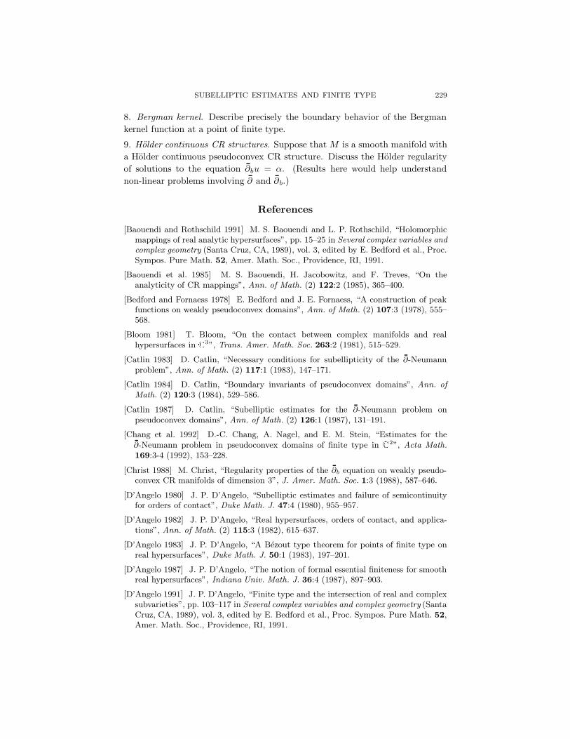
8. Bergman kernel. Describe precisely the boundary behavior of the Bergmankernel function at a point of finite type.
9. Holder continuous CR structures. Suppose that M is a smooth manifold witha Holder continuous pseudoconvex CR structure. Discuss the Holder regularityof solutions to the equation ∂bu = α. (Results here would help understandnon-linear problems involving ∂ and ∂b.)
References
[Baouendi and Rothschild 1991] M. S. Baouendi and L. P. Rothschild, “Holomorphicmappings of real analytic hypersurfaces”, pp. 15–25 in Several complex variables andcomplex geometry (Santa Cruz, CA, 1989), vol. 3, edited by E. Bedford et al., Proc.Sympos. Pure Math. 52, Amer. Math. Soc., Providence, RI, 1991.
[Baouendi et al. 1985] M. S. Baouendi, H. Jacobowitz, and F. Treves, “On theanalyticity of CR mappings”, Ann. of Math. (2) 122:2 (1985), 365–400.
[Bedford and Fornaess 1978] E. Bedford and J. E. Fornaess, “A construction of peakfunctions on weakly pseudoconvex domains”, Ann. of Math. (2) 107:3 (1978), 555–568.
[Bloom 1981] T. Bloom, “On the contact between complex manifolds and realhypersurfaces in C
3”, Trans. Amer. Math. Soc. 263:2 (1981), 515–529.
[Catlin 1983] D. Catlin, “Necessary conditions for subellipticity of the ∂-Neumannproblem”, Ann. of Math. (2) 117:1 (1983), 147–171.
[Catlin 1984] D. Catlin, “Boundary invariants of pseudoconvex domains”, Ann. ofMath. (2) 120:3 (1984), 529–586.
[Catlin 1987] D. Catlin, “Subelliptic estimates for the ∂-Neumann problem onpseudoconvex domains”, Ann. of Math. (2) 126:1 (1987), 131–191.
[Chang et al. 1992] D.-C. Chang, A. Nagel, and E. M. Stein, “Estimates for the
∂-Neumann problem in pseudoconvex domains of finite type in C2”, Acta Math.
169:3-4 (1992), 153–228.
[Christ 1988] M. Christ, “Regularity properties of the ∂b equation on weakly pseudo-convex CR manifolds of dimension 3”, J. Amer. Math. Soc. 1:3 (1988), 587–646.
[D’Angelo 1980] J. P. D’Angelo, “Subelliptic estimates and failure of semicontinuityfor orders of contact”, Duke Math. J. 47:4 (1980), 955–957.
[D’Angelo 1982] J. P. D’Angelo, “Real hypersurfaces, orders of contact, and applica-tions”, Ann. of Math. (2) 115:3 (1982), 615–637.
[D’Angelo 1983] J. P. D’Angelo, “A Bezout type theorem for points of finite type onreal hypersurfaces”, Duke Math. J. 50:1 (1983), 197–201.
[D’Angelo 1987] J. P. D’Angelo, “The notion of formal essential finiteness for smoothreal hypersurfaces”, Indiana Univ. Math. J. 36:4 (1987), 897–903.
[D’Angelo 1991] J. P. D’Angelo, “Finite type and the intersection of real and complexsubvarieties”, pp. 103–117 in Several complex variables and complex geometry (SantaCruz, CA, 1989), vol. 3, edited by E. Bedford et al., Proc. Sympos. Pure Math. 52,Amer. Math. Soc., Providence, RI, 1991.

230 JOHN P. D’ANGELO AND JOSEPH J. KOHN
[D’Angelo 1993] J. P. D’Angelo, Several complex variables and the geometry of realhypersurfaces, Studies in Advanced Mathematics, CRC Press, Boca Raton, FL, 1993.
[D’Angelo 1995] J. P. D’Angelo, “Finite type conditions and subelliptic estimates”,pp. 63–78 in Modern methods in complex analysis (Princeton, 1992), edited by T.Bloom et al., Annals of Mathematics Studies 137, Princeton Univ. Press, Princeton,NJ, 1995.
[Diederich and Fornaess 1978] K. Diederich and J. E. Fornaess, “Pseudoconvex domainswith real-analytic boundary”, Ann. of Math. (2) 107:2 (1978), 371–384.
[Fefferman 1995] C. Fefferman, “On Kohn’s microlocalization of ∂ problems”, pp. 119–133 in Modern methods in complex analysis (Princeton, 1992), edited by T. Bloomet al., Annals of Mathematics Studies 137, Princeton Univ. Press, Princeton, NJ,1995.
[Fefferman and Kohn 1988] C. L. Fefferman and J. J. Kohn, “Holder estimates ondomains of complex dimension two and on three-dimensional CR manifolds”, Adv.in Math. 69:2 (1988), 223–303.
[Fefferman et al. 1990] C. L. Fefferman, J. J. Kohn, and M. Machedon, “Holderestimates on CR manifolds with a diagonalizable Levi form”, Adv. in Math. 84:1(1990), 1–90.
[Folland and Kohn 1972] G. B. Folland and J. J. Kohn, The Neumann problem forthe Cauchy-Riemann complex, Annals of Mathematics Studies 75, Princeton Univ.Press, Princeton, NJ, 1972.
[Fornæss and Sibony 1991] J. E. Fornæss and N. Sibony, “On Lp Estimates for ∂”, pp.129–163 in Several complex variables and complex geometry (Santa Cruz, CA, 1989),vol. 3, edited by E. Bedford et al., Proc. Sympos. Pure Math. 52, Amer. Math. Soc.,Providence, RI, 1991.
[Greiner 1974] P. Greiner, “Subelliptic estimates for the δ-Neumann problem in C2”,
J. Differential Geometry 9 (1974), 239–250.
[Guan 1990] P. Guan, “Holder regularity of subelliptic pseudodifferential operators”,Duke Math. J. 60:3 (1990), 563–598.
[Ho 1991] L.-H. Ho, “Subelliptic estimates for the ∂-Neumann problem for n−1 forms”,Trans. Amer. Math. Soc. 325:1 (1991), 171–185.
[Hormander 1966] L. Hormander, An introduction to complex analysis in severalvariables, Van Nostrand, Princeton, NJ, 1966.
[Kohn 1963] J. J. Kohn, “Harmonic integrals on strongly pseudo-convex manifolds, I”,Ann. of Math. (2) 78 (1963), 112–148.
[Kohn 1964] J. J. Kohn, “Harmonic integrals on strongly pseudo-convex manifolds,II”, Ann. of Math. (2) 79 (1964), 450–472.
[Kohn 1972] J. J. Kohn, “Boundary behavior of δ on weakly pseudo-convex manifoldsof dimension two”, J. Differential Geometry 6 (1972), 523–542.
[Kohn 1977] J. J. Kohn, “Methods of partial differential equations in complex analysis”,pp. 215–237 in Several complex variables (Williamstown, MA, 1975), vol. 1, editedby R. O. Wells, Jr., Proc. Sympos. Pure Math. 30, Amer. Math. Soc., 1977.
[Kohn 1979] J. J. Kohn, “Subellipticity of the ∂-Neumann problem on pseudo-convexdomains: sufficient conditions”, Acta Math. 142:1-2 (1979), 79–122.

SUBELLIPTIC ESTIMATES AND FINITE TYPE 231
[Kohn 1984] J. J. Kohn, “A survey of the ∂-Neumann problem”, pp. 137–145 inComplex analysis of several variables (Madison, WI, 1982), edited by Y.-T. Siu,Proc. Symp. Pure Math. 41, Amer. Math. Soc., Providence, RI, 1984.
[Kohn 1985] J. J. Kohn, “Estimates for ∂b on pseudoconvex CR manifolds”, pp. 207–217 in Pseudodifferential operators and applications (Notre Dame, IN, 1984), editedby F. Treves, Proc. Symp. Pure Math. 43, Amer. Math. Soc., Providence, 1985.
[Kohn 1986] J. J. Kohn, “The range of the tangential Cauchy–Riemann operator”,Duke Math. J. 53:2 (1986), 525–545.
[Kohn and Nirenberg 1965] J. J. Kohn and L. Nirenberg, “Non-coercive boundaryvalue problems”, Comm. Pure Appl. Math. 18 (1965), 443–492.
[Kohn and Nirenberg 1973] J. J. Kohn and L. Nirenberg, “A pseudo-convex domainnot admitting a holomorphic support function”, Math. Ann. 201 (1973), 265–268.
[Lewy 1956] H. Lewy, “On the local character of the solutions of an atypical lineardifferential equation in three variables and a related theorem for regular functionsof two complex variables”, Ann. of Math. (2) 64 (1956), 514–522.
[McNeal 1989] J. D. McNeal, “Boundary behavior of the Bergman kernel function inC2”, Duke Math. J. 58:2 (1989), 499–512.
[McNeal 1992] J. D. McNeal, “Convex domains of finite type”, J. Funct. Anal. 108:2(1992), 361–373.
[McNeal and Stein 1994] J. D. McNeal and E. M. Stein, “Mapping properties of theBergman projection on convex domains of finite type”, Duke Math. J. 73:1 (1994),177–199.
[Nagel et al. 1989] A. Nagel, J.-P. Rosay, E. M. Stein, and S. Wainger, “Estimates forthe Bergman and Szego kernels in C
2”, Ann. of Math. (2) 129:1 (1989), 113–149.
[Rothschild and Stein 1976] L. P. Rothschild and E. M. Stein, “Hypoelliptic differentialoperators and nilpotent groups”, Acta Math. 137:3-4 (1976), 247–320.
[Shaw 1985] M.-C. Shaw, “L2-estimates and existence theorems for the tangentialCauchy–Riemann complex”, Invent. Math. 82:1 (1985), 133–150.
[Sibony 1991] N. Sibony, “Some aspects of weakly pseudoconvex domains”, pp. 199–231 in Several complex variables and complex geometry (Santa Cruz, CA, 1989),vol. 1, edited by E. Bedford et al., Proc. Sympos. Pure Math. 52, Amer. Math.Soc., Providence, RI, 1991.
[Stanton 1996] N. K. Stanton, “Infinitesimal CR automorphisms of real hypersurfaces”,Amer. J. Math. 118:1 (1996), 209–233.
[Sweeney 1972] W. J. Sweeney, “Coerciveness in the Neumann problem”, J. DifferentialGeometry 6 (1972), 375–393.
[Trepreau 1986] J.-M. Trepreau, “Sur le prolongement holomorphe des fonctions C–Rdefines sur une hypersurface reelle de classe C2 dans C n”, Invent. Math. 83:3 (1986),583–592.
[Tumanov 1988] A. E. Tumanov, “Extending CR functions on manifolds of finite typeto a wedge”, Mat. Sb. (N.S.) 136(178):1 (1988), 128–139. In Russian; translated inMath. USSR Sb. 64:1 (1989), 129–140.
[Yu 1994] J. Y. Yu, “Peak functions on weakly pseudoconvex domains”, Indiana Univ.Math. J. 43:4 (1994), 1271–1295.

232 JOHN P. D’ANGELO AND JOSEPH J. KOHN
John P. D’Angelo
Deptartment of Mathematics
University of Illinois
Urbana, IL 61801
United States
Joseph J. Kohn
Deptartment of Mathematics
Princeton University
Princeton, NJ 08540
United States


![Math. Ann. 312, 341–362 (1998) Mathematische Annalenhajlasz/OriginalPublications/HajlaszSt-Subelliptic... · [74], Vodop’yanov and Chernikov [75], Vodop’yanov and Markina [76],](https://static.fdocuments.in/doc/165x107/5f06bab47e708231d419714a/math-ann-312-341a362-1998-mathematische-hajlaszoriginalpublicationshajlaszst-subelliptic.jpg)