Subcontracting and Competitive Bidding on IncompleteProcurement Contracts

Daniel P. Miller∗

Clemson University

March 15, 2011

Abstract

This paper examines the impact of incomplete contracts on subcontracting arrange-ments and the design of procurement auctions. I examine 2,200 individual components(i.e. drilling, concrete, traffic striping) on 32 bridge projects procured by the CaliforniaDepartment of Transportation. I use ex-post revisions to construct a measure of con-tractual incompleteness. I model a scoring auction that shows how ex-post revisionsaffect bidding decisions and derive an approach to estimate the individual cost compo-nents using a sieve estimator. Regarding auction design, I propose an improved scoringrule and quantify the welfare benefits. Regarding subcontracting, the results provideone of the first pieces of quantitative evidence supporting the incomplete contractingtheories of the firm.

1 Introduction

Construction contracts are incomplete because they are affected by random shocks, whether it is

an unknown site condition, deficiency in the design, or external environmental factor. Boston’s Big

Dig is a highly publicized project that was riddled by such shocks. By their very nature, these

unpredictable events are non-contractible. But, contractors bidding on projects are acutely aware

that these sorts of things can happen and are mindful of the consequences. Contractors take them

into account when making bidding and subcontracting decisions.

In this paper I consider the impact of incomplete contracts on subcontracting arrangements

and the design of procurement auctions for public infrastructure projects. The goal is two fold.

First, I quantify how measures of contractual incompleteness affect contractor’s costs, and moreover

separate the cost effects for both subcontracting and in-house arrangements.

∗Author correspondence: dmille7@g.clemson.edu

1

Second, I show how the same sort of incompleteness distorts bidding strategies in the competitive

bidding mechanism most commonly used by departments of transportation to procure highways and

bridges. After laying out the auction theory, I propose a structural estimation technique that allows

me to empirical evaluate the importance of these distortions. I then propose a simple modification

to the auction design that could improve outcomes for bidders and save money for procurement

agencies.

Regarding the first objective of this paper, there is a large theoretical and empirical literature

about incomplete contracts and the make or buy literature. The predictions about the make or buy

decision in the incomplete contracting literature Coase (1937); Williamson (1985); Grossman and

Hart (1986); Hart and Moore (1990, 2008), are based on a trade-off between cost savings incentives

and the potential for hold up costs. While subcontracting arrangements have the advantage over in-

house contracting arrangements by providing high powered incentives to keep costs down, they may

suffer more severe hold-up problems and costly renegotiation in contracting environments marked

by a high degree of incompleteness. As stated by Sweet (2004) a legal scholar on construction

contracts, these tradeoffs make subcontracting the ”Achilles Heel” of construction. Given that

about 50% of work is subcontracted in the public, the cost of incompleteness could potentially be

quite large.

This paper distinguishes itself from others in the make or buy literature because data on bids

allows me to draw inference on cost and provide quantitative evidence. Other studies only provide

qualitative evidence. That is, they show how some feature of the theory (such as incompleteness)

affects the probability that work is subcontracted. There is very little quantitative evidence about

the impact of firm boundaries on economic outcomes such as cost. The lack of quantitative evidence

has been a major critique in this literature (Hubbard, 2008; Lafontaine and Slade, 2007; Klein,

2005). This paper offers one of the first attempts to bring the missing data, examine the cost

primitives of the theory, and, stated bluntly, to show that firm boundaries matter.

The empirical strategy uses data on bids and a measure of incompleteness to estimate the effect

of incompleteness on cost for both subcontracting and in-house contracting arrangements. For

each project, the bids are broken down by components that range from laying asphalt or pouring

concrete, to striping traffic lanes or installing landscaping. In total there are over 2200 components

across the 32 projects in the data set. Component bids are submitted as unit price bids (i.e. dollars

per yard of concrete) that reflect bidder’s unit cost. The original plans on the project call for a

quantity on each item, but external shocks (which I interpret as the source of incompleteness) can

cause the ex-post quantities installed to differ from the original quantities. I measure the degree

of incompleteness using difference in original and ex-post quantities. The idea is that by observing

a large change, the bidding contractors likely forecast that component would be prone to changes.

The baseline empirical model regresses unit prices bids on the quantity changes to estimate the

effect of incompleteness. But, this baseline specification is biased because quantity changes induce

2

bidders to distort their unit price bids from cost.

To understand the second objective of the paper, bidding strategies and auction design, it’s

worthwhile considering the auction mechanism in more detail. These are scoring auctions. To

determine the low bidder and winner of the auction, each of the unit price bids are multiplied with

the corresponding quantity from the original plans and summed across items. That is, the bids

are scored using the original quantities. Payments are based on the revised quantities actually

installed. The difference between how bids are scored and how they are paid means bidders receive

final payments that can differ from their original bids. For example, a bidder receives extra payment

if quantities overrun and less if quantities underrun.

As shown by Athey and Levin (2001), this auction mechanism induces bidders to skew their

bids away from cost. The basic intuition shows that bidders skew unit price bids above cost on

tasks expected to overrun on quantity and below cost on tasks expected to underrun. By skewing,

a bidder earns a higher profit without affecting its total bid and hence probability of winning the

project. Bid skewing is risky. If the overrun (or, for that matter underrun) does not occur, the

winning bidder suffers a loss. The principles for allocating unit price bids are analogous to concepts

from modern portfolio theory (Markowitz, 1952). The specific modeling choices match industry

practitioners’ intuition about unit price bidding. They credit these ideas to Gates (1959). I appy

results from the scoring auction literature to formally characterize equilibrium bidding behavior

(Asker and Cantillon, 2008).

As multi-dimensional auctions, the estimation procedure estimates individual unit costs, not

the total cost on the project. From the first order conditions to optimal bidding, I propose a

sieve estimator that maps bids to costs and accounts for bid skewing. The sieve basis relate the

magnitude of a skew to the variance of quantity changes on the component, and the covariance of

quantity changes with other components. The sieve estimator not only corrects the confounding

effects of bid skewing for incompleteness regression, but it also recovers the correlation structure of

bid skewing. With these estimates, I can assess the magnitude of skewing.

Bid skewing has two welfare consequences. First, there is a loss in efficiency because the procurer

is paying at rates that differ from the contractor’s cost. Second, bidder’s are exposed to additional

risk because they are skewing. I propose an improvement in the scoring rule design that eliminates

incentives to skew. The department of transportation is myopic with its scoring rule. They base

quantities off of some original plans, and don’t take into account the possibility that quantities can

change. By forecasting quantities in the same ways bidders do, they can adjust the scoring weights

to be in line with contractors forecasts. If the scoring rule perfectly aligns the scored quantities

with expectations of actual quantities, bidders won’t skew. In the counterfactual, I quantify the

benefits of this alternative scoring rule.

3

1.1 Contribution to Existing Literature

This study joins an emerging literature that quantifies the impact of firm boundaries on economic

outcomes. Recent examples include Gil (2008) (industry : cinemas and performance outcome: movie

run length), Ciliberto (2006) (hospitals and capital investments), Forbes and Lederman (2008)

(airlines and flight delays), and Novak and Stern (2008) (automobiles and consumer quality ratings).

Others—Baker and Hubbard (2004) (trucking and fuel economy) and Levin and Tadelis (2008)

(municipal services and city expenditures)—consider but do not focus on performance outcomes.

This application offers several advantages. First, I am making inference on the most relevant

economic outcome: costs. In the incomplete contracting theories, cost determines “make or buy”

decisions. The performance outcomes in the other studies, although interesting, are not direct

determinants. Second, the auction format provides a crisp separation between ex-ante contract

formation and ex-post contract execution. The theories predict that both ex-ante costs of incentive

distortions and ex-post bargaining and renegotiations costs are relevant factors in the make-or-buy

decision. A forward looking, rational contractor will incorporate both types of costs in his bid.

Thus, I capture the combination of both types of costs. 1 Third, the structural approach makes it

possible to conduct counterfactual exercises. As part of a cost-benefit analysis, one could quantify

Caltrans’ costs savings if it were to reduce contractual incompleteness. I could alter regulations

that distort subcontracting patterns.2

This study falls into the class of empirical work that considers the uncertainty and complex-

ity of a transaction. Seminal contributions include Monteverde and Teece (1982), Masten (1984),

and Masten, Meehan Jr, and Snyder (1991). They find a higher degree of complexity is associ-

ated with a lower probability of subcontracting. Recent work by Gil (2007) (movies), Acemoglu,

Aghion, Griffith, and Zilibotti (2009) (R&D intensity), Forbes and Lederman (2009) (airlines)

Levin and Tadelis (2008) (municipal services) obtain the same result. The literature on forward

integration into retailing finds mixed evidence.3 Williamson (1985) and, in particular, his earlier

work Williamson (1975), identified uncertainty as one of the key determinants of firm boundaries

for empirical researchers to take to the data.4 This factor is losing favor, in part, because of the

difficulty of measuring uncertainty. Typically, studies rely on survey data of industry practitioners

or measures of market volatility. These variables are notoriously measured with error, causing se-

vere attenuation bias and statistically insignificant estimates.5 A strength of this study is that the

1There has been a call in the literature by Whinston (2003) to distinguish between the transactions cost(Williamson, 1985) and property rights theories (Hart and Moore, 1990). The distinction hinges on theability to separately identify the two channels of contracting costs. I do not attempt to do so in this paper.

2These counterfactuals are outside the scope of this paper.3See Lafontaine and Slade (2007) for a survey of these results.4Holmstrom and Roberts (1998) provide this textual interpretation. The other two are specificity and

frequency of a transaction.5Klein (2005) notes the problem of measurement error in these types of studies.

4

measurement captures a precise notion of contractual incompleteness: changes in the construction

plans measured at the detailed level of a work item transaction.

This work is related to the empirical auctions literature. There is an especially large body of

work on highway procurement auctions including the contributions of Porter and Zona (1993), Hong

and Shum (2002), Krasnokutskaya (2009), Jofre-Bonet and Pesendorfer (2003), Bajari, Houghton,

and Tadelis (2007), Marion (2008), De Silva et al. (2008), and Krasnokutskaya (2009). This paper

distinguishes itself because it estimates cost on individual components of the multi-dimensional

auctions, rather than treating the auctions as single dimensional first price auctions. A 6 Bajari

and Lewis (2008) consider the design of procurement auctions with a time-to-completion component

of the bid. Their modeling and empirical methods share similarities with the approach in this paper.

Previous empirical work on bid skewing (Athey and Levin, 2001; Bajari et al., 2007) restricted

attention to just one dimension of skewing. I model the bid skewing decision as a portfolio choice

problem. That is, the correlation structure in quantity change risk across all tasks determines

the optimal skew on any given task. The proposed empirical technique recovers the correlation

structure of risk. Risk aversion in auctions has attracted attention in both the empirical auctions

and experimental economics literature.7 Adapting the method could provide field evidence on

measures of risk aversion with millions of dollars at stake.

The paper is organized as follows; section 2 describes the procurement process and follows

with a discussion in section 3. Section 4 presents the model and characterizes optimal bidding and

subcontracting decisions. Section 5 describes the data; section 6, the estimation procedure. Section

7 presents results. Section 8 discusses robustness; section 9 concludes.

2 Procurement Process

Caltrans procures projects using a method called Design-Bid-Build. It is the most common method

used by departments of transportation. The name refers to the three stages of the process. Below

I outline the timing, introduce notation, and describe the auction mechanism.

Design Caltrans’ resident engineers write blueprints and specifications. They include T tasks

indexed t = 1, . . . , T . Examples include concrete, steel, excavation, and traffic striping.

Caltrans employs a team of specialists called quantity surveyors. They examine the plans

and calculate quantities for each task qet (in vector notation qe = [qe1, qe2, . . . , q

eT ]).8 Primary

6Marion (2008) is closely related to this paper on two dimensions. He studies a California affirmativeaction law regarding highway subcontracting. He uses work item observations but does not account for bidskewing.

7See Campo, Guerre, Perrigne, and Vuong (2003), and Harrison and Rutstrom (2008) for discussions.8For convenience many variables are expressed as vectors with length T . These variables will unambigu-

ously be denoted in boldface.

5

contractors and subcontractors inspect blueprints and the job-site to forecast costs. They do

not participate in the design process.

Sign Subcontracts Before bids are submitted, bidding primary contractors, indexed i = 1, . . . , N ,

choose subcontracting arrangements. Let csit denote primary contractor i’s unit cost to sub-

contract task t, and cpit denote its unit cost to perform the task in-house.

For most tasks there are many potential subcontractors and the selection process is quite

competitive. Matching of subcontractors with primary contractors is not exclusive. A sub-

contractor can sign with multiple prime contractors. By law, California’s Subletting and

Subcontracting Fair Practice Act,9 stipulates that subcontract agreements must be signed

before bidding. After a project has been awarded, the winning prime contractor cannot

legally hire additional subcontractors, nor can it make substitutions.

Bid Each bidding prime contractor submits sealed unit price bids for every task. Let bit denote

bidder i’s unit price bid on task t (in vector notation bi). The unit price bids are scored by

multiplying unit price bids with the corresponding quantity in the engineer’s original plans

and summing across all task: si = bi ·qe. The bidder with the lowest score si is awarded the

entire project.

Build This is the ex-post period when the project is constructed. During this phase contingen-

cies can arise which will require revisions of the plans. Many of these revisions necessitate

adjustments to quantities. Quantity surveyors re-examine the revised plans to authorize the

actual quantities. Denote the quantity actually installed after revisions for task t as qat (in

vector notation qa).

Payment to the winning bidder is based on quantities actually installed: bi · qa. Losing

bidders do not receive payment. It is important to note that contractors do not choose

actual quantities. From their perspective, actual quantities and payments are a random

variable.

3 Discussion: Contracts and Incompleteness

I focus on the contracting relationship between prime contractors and subcontractors, or if work

is not subcontracted, between prime contractors and direct suppliers of inputs (labor, material,

9California was the first state to adopt this law, 10 other states have followed. It is intended to preventthe practice of post award bid shopping; it prevents winning prime contractors from exercising monopsonypower to garner price concessions from subcontractors. For transparency, the law requires bidding contractorsto furnish to the public procuring agency the names, addresses, and lists of work to be performed for allsubcontractors with its bid submittal. The public information disclosure is one reason why Caltrans contractswere chosen for this study.

6

equipment). Caltrans, the buyer, is a relevant third party that might exacerbate hold-up problems,

but is not the focus.10 Subcontracts and in-house contracts (with direct suppliers) differ. The

standard pricing terms in subcontracts are very simple: a fixed unit price bid. In this sense,

subcontracts resemble fixed price contracts that have the benefit of providing subcontractors with

strong incentives to make non-contractible, relationship specific investments into cost reduction.

Other, non-price, performance terms in subcontracts are much more complex. Examples, include

coordinating schedules, assigning monitoring duties, preparing mechanisms to resolve conflicts.

Explicitly spelling out contingencies surrounding these terms can be quite costly, particularly for

tasks characterized by a high degree of complexity. As such, many will be left out. If there

is a revision, and something different must be built, many of these performance terms must be

renegotiated. This is the downside to subcontracting; ex-post renegotiation dissipates surplus,

and/or diminishes incentives to make relationship specific investments.

It is standard in the literature on construction contracting (Bajari and Tadelis, 2001) to treat

in-house contracts as more closely resembling cost-plus contracts with input suppliers. The prime

contractor rents inputs at cost, plus a negotiated mark-up. These contracts provide less incentive to

reduce cost, but have the advantage of being more flexible in accommodating revisions and require

less up-front cost to spell out contingencies.

It is also worth noting the importance of relational contracting in this industry. Repeated past

relationships, and prospects of future business, can mitigate many of the bargaining frictions and

enhance cost reducing incentives. Repeated contracting may be important in relationships with

both subcontractors and direct suppliers. In the interpretation of results, I further elaborate on

the elements of subcontracts, input supplier contracts, and relational contracts as they pertain to

certain types of tasks and revisions.

I use observed revisions to the construction plans to measure the degree of complexity and

incompleteness in contracts. Specifically, I use the difference in original quantities, qet , and quantities

installed after revisions, qat . To illustrate the link between plan revisions, quantity changes, and the

underlying source of complexity and incompleteness, consider an example about the most drastic

change from the reconstruction of the collapsed 35W bridge in Minneapolis.11 The right pane

in figure 1 shows a photo of the completed bridge, and the left pane shows a photo from the

construction of the piers. The piers support the far side of the bridge. Contractors recognized the

complexity and incompleteness of this project. It was complex because the worksite was located

in an urban area, littered with debris from the collapsed bridge, and abutted a fast-moving river.

Plans preparation was particularly incomplete because it was a fast-tracked project. As it turned

out, a major revision was made because of an unaccounted for drainage system located at the base

10See Bajari et al. (2007) for further discussion of Caltrans’ design-bid-build contracts and hold-up withCaltrans.

11The original structure collapsed August 1st, 2007.

7

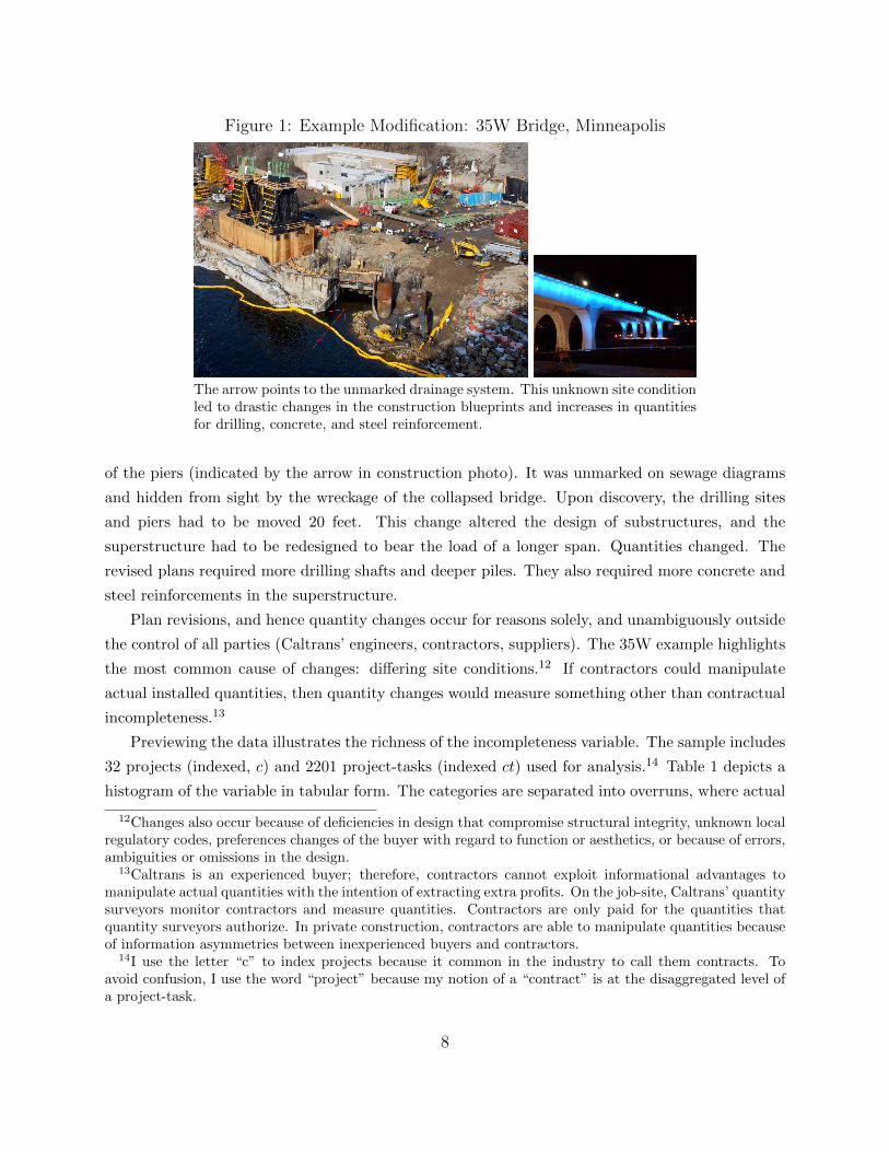
Figure 1: Example Modification: 35W Bridge, Minneapolis

The arrow points to the unmarked drainage system. This unknown site conditionled to drastic changes in the construction blueprints and increases in quantitiesfor drilling, concrete, and steel reinforcement.

of the piers (indicated by the arrow in construction photo). It was unmarked on sewage diagrams

and hidden from sight by the wreckage of the collapsed bridge. Upon discovery, the drilling sites

and piers had to be moved 20 feet. This change altered the design of substructures, and the

superstructure had to be redesigned to bear the load of a longer span. Quantities changed. The

revised plans required more drilling shafts and deeper piles. They also required more concrete and

steel reinforcements in the superstructure.

Plan revisions, and hence quantity changes occur for reasons solely, and unambiguously outside

the control of all parties (Caltrans’ engineers, contractors, suppliers). The 35W example highlights

the most common cause of changes: differing site conditions.12 If contractors could manipulate

actual installed quantities, then quantity changes would measure something other than contractual

incompleteness.13

Previewing the data illustrates the richness of the incompleteness variable. The sample includes

32 projects (indexed, c) and 2201 project-tasks (indexed ct) used for analysis.14 Table 1 depicts a

histogram of the variable in tabular form. The categories are separated into overruns, where actual

12Changes also occur because of deficiencies in design that compromise structural integrity, unknown localregulatory codes, preferences changes of the buyer with regard to function or aesthetics, or because of errors,ambiguities or omissions in the design.

13Caltrans is an experienced buyer; therefore, contractors cannot exploit informational advantages tomanipulate actual quantities with the intention of extracting extra profits. On the job-site, Caltrans’ quantitysurveyors monitor contractors and measure quantities. Contractors are only paid for the quantities thatquantity surveyors authorize. In private construction, contractors are able to manipulate quantities becauseof information asymmetries between inexperienced buyers and contractors.

14I use the letter “c” to index projects because it common in the industry to call them contracts. Toavoid confusion, I use the word “project” because my notion of a “contract” is at the disaggregated level ofa project-task.

8

Table 1: Quantity Overruns and Underrunsqat−qetqet

Frequency

Perfect Design 0 35.4%

OverrunsSmall (0,.1] 11.0%Medium (.1,.35] 7.2%Large >.35 10.0%

UnderrunsSmall [-.1,0) 13.6%Medium [-35,-.1) 8.4%Large [-1,-.35) 14.3%

Projects 32Project-task Observations 2201

quantities are larger than original quantities and underruns, where actual quantities are less than

original quantities. The size of changes are divided into 4 categories: large, medium and small

changes, and a category labeled, “perfect design” that corresponds to no change. First, notice that

this is a continuous measure and not a crude indicator for whether or not a task experienced a

change. Also notice the large degree of variation. Contractors and Caltrans consider changes of

25% to be quite large. It is remarkable that a fourth of the tasks experience changes exceeding 35%.

Finally, notice the separation of overruns and underruns. This distinction allows me to distinguish

between types of hold-up problems. For example, overruns can trigger hold-up problems related to

scheduling and accelerating the pace of work. I elaborate in the results section.

It is also worth elaborating on the jobs of Caltrans’ engineers and quantity surveyors. The

original quantities are not a guess, or expectation, of what actual quantities will turn out to be.

Formally qe 6= E[qa]. Engineers write plans, and, if need be, revise plans. Quantity surveyors

calculate quantities from the original plans, and if need be, calculate quantities from revised plans.

Quantity surveyors are trained to be exact; human error on the part of quantity surveyors does not

cause quantity changes.

The incompleteness variable is measured with error because it uses ex-post data. Ideally, I

would observe bidders’ expectations about revisions at the time of bidding. Since I do not observe

expectations of actual quantities E[qat ], I use the realized outcome qat . This introduces expectational

error. I address the implications of this form of measurement error in the econometrics and results

sections.

3.1 Baseline Empirical Specification

For the moment, suppose as the econometrician I either observe costs csit and cpit directly or assume

unit price bids equal cost bit = cit. I can estimate the effect of incompleteness, measured as absolute

deviations of quantity changes incit =∣∣∣ qat−qetqat

∣∣∣ on cost using the following specification for cost,

9

bitp = x′itpβ0p + βinc0p inct + eitp (1)

bits = x′itsβ0s + βinc0s inct + eits (2)

The subscripts p and s reference work performed by the prime contractor and subcontractor,

x is a set of cost shifts, and e are unobserved cost shocks. There are econometric issues regarding

selection bias in subcontracting decisions; those are further discussed in the econometrics specifi-

cation.

4 Model of Subcontracting and Competitive Bidding

In this section, I model and characterize prime contractors’ bidding decisions. I further discuss the

auction because there is an important strategic reason for unit price bids to differ from unit cost.

Like the incompleteness variable, bid skewing strategies depends on quantity changes. Failing to

account for bid skewing gives biased estimates of the parameters in equation 1.

4.1 Bid Skewing Strategies: Example

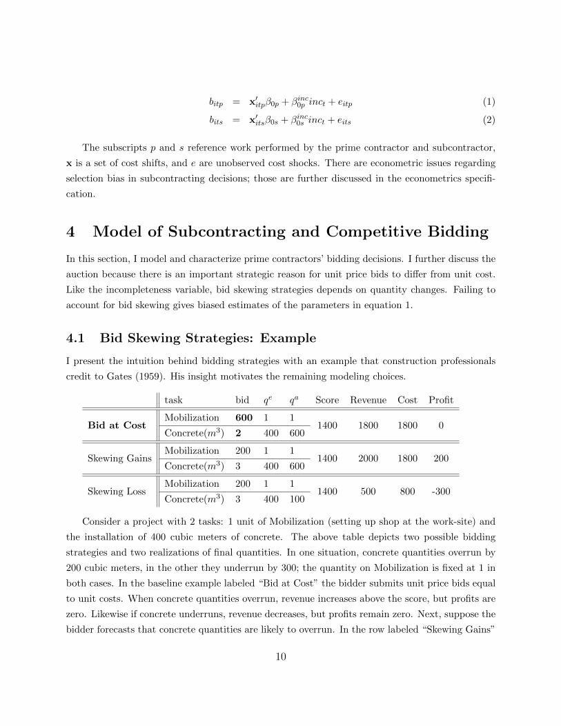
I present the intuition behind bidding strategies with an example that construction professionals

credit to Gates (1959). His insight motivates the remaining modeling choices.

task bid qe qa Score Revenue Cost Profit

Bid at CostMobilization 600 1 1

1400 1800 1800 0Concrete(m3) 2 400 600

Skewing GainsMobilization 200 1 1

1400 2000 1800 200Concrete(m3) 3 400 600

Skewing LossMobilization 200 1 1

1400 500 800 -300Concrete(m3) 3 400 100

Consider a project with 2 tasks: 1 unit of Mobilization (setting up shop at the work-site) and

the installation of 400 cubic meters of concrete. The above table depicts two possible bidding

strategies and two realizations of final quantities. In one situation, concrete quantities overrun by

200 cubic meters, in the other they underrun by 300; the quantity on Mobilization is fixed at 1 in

both cases. In the baseline example labeled “Bid at Cost” the bidder submits unit price bids equal

to unit costs. When concrete quantities overrun, revenue increases above the score, but profits are

zero. Likewise if concrete underruns, revenue decreases, but profits remain zero. Next, suppose the

bidder forecasts that concrete quantities are likely to overrun. In the row labeled “Skewing Gains”

10

the bidder skews the unit price bid on concrete above unit cost, and below cost on Mobilization.

Revenue and profit increase as compared to a strategy of bidding at cost, yet, the bidder maintains

the same score, thereby not diminishing its chances of winning the auction. Such a strategy comes

with risk as the row labeled “Skewing Loss” illustrates. If the concrete quantity underruns, the

bidder suffers a loss of profits. Gates (1959) intuition is about the risk-reward tradeoff of skewing

bids away from cost.

4.2 Continued Auction Description

I model the auction in the independent private values paradigm. Bidder i’s costs are drawn from

the joint density, fi(csi , c

pi |I) with compact, convex support on RT+×RT+. Densities may differ across

bidders, but it is assumed they share common support. Furthermore, the cost draws are independent

across bidders conditional on publicly observed information at the time of bidding I. In this model,

bidder’s choose that lowest cost subcontracting arrangement on each task: cit = min{csit, cpit}

Actual quantities are drawn from the joint density g(qa). Realization of the draw occurs after

bidding. Ex-ante bidders have identical information about this density.15 Later, I will make use of

an assumption that E[(qa − qe)′(qa − qe)] has full rank. This expression resembles a covariance

matrix of quantity overruns and underruns.

Following the intuition of Gates’ example, bidders are modeled to exhibit risk aversion over

profits.16 Let bidders have identical utility over profits, represented by a twice continuously differ-

entiable, increasing, strictly concave utility function u(·).The expected utility of a bidder if it wins the project is Eqa [u (π(bi, ci;q

a))] where the ex-

pectation is integrated across possible realizations of actual quantities. This value is normalized

to zero for losing bidders. Bidder i’s payoff is its expected utility if it wins the auction times the

probability it wins the auction.

Eqa [u (π(bi, ci,qa))]× Pr(si < sj ∀j 6= i)

15Athey and Levin (2001) analyze timber auctions where a similar phenomenon occurs. The amountof timber species bid on and harvested differs. A model with affiliated signals about actual quantities isappropriate in their setting because bidders sample only small portions of a forest. In this application allbidders inspect exactly the same plans and job site so it is not clear why they would receive different signalsabout installed quantities. Furthermore modeling a general affiliated values auction makes formal analysisintractable with more than two tasks.

16That contractors are risk averse is well justified. First, industry practitioners, such as Gates, acknowledgetheir risk aversion. Second, contractors are highly leveraged, have small profit margins, and operate at asmall scale. Excessively risky bidding behavior could trigger a default on a performance bond or causebankruptcy.

11

4.3 Characterization of Bidding

The equilibrium concept for this auction is a Bayesian Nash equilibrium. Bidders select unit price

bids that are best responses to the equilibrium distribution of opponents’ bids. A best response

solves the following maximization problem

maxbi∈RT

+

Eqa [u ((bi − ci) · qa)]×H(si)

H(si) = Pr(si < sj ∀j 6= i)

sj opponent j’s equilibrium score

where sj is the equilibrium score for some type of opponent j. The choice of bids can be broken

down into two parts. In the first part, bidders choose an optimal score, si, that is a best response

to their rivals’ scores. In the second part, bidders allocate unit price bids subject to the constraint

that they sum to the chosen score, bi · qe = si. The formal statement of this claim and proof are

presented in Proposition 1 in the appendix.

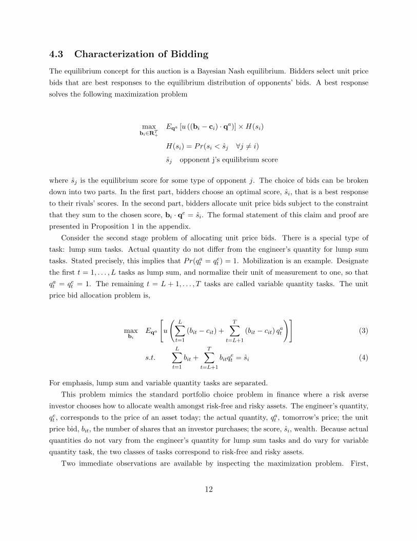
Consider the second stage problem of allocating unit price bids. There is a special type of

task: lump sum tasks. Actual quantity do not differ from the engineer’s quantity for lump sum

tasks. Stated precisely, this implies that Pr(qat = qet ) = 1. Mobilization is an example. Designate

the first t = 1, . . . , L tasks as lump sum, and normalize their unit of measurement to one, so that

qat = qet = 1. The remaining t = L + 1, . . . , T tasks are called variable quantity tasks. The unit

price bid allocation problem is,

maxbi

Eqa

[u

(L∑t=1

(bit − cit) +

T∑t=L+1

(bit − cit) qat

)](3)

s.t.L∑t=1

bit +T∑

t=L+1

bitqet = si (4)

For emphasis, lump sum and variable quantity tasks are separated.

This problem mimics the standard portfolio choice problem in finance where a risk averse

investor chooses how to allocate wealth amongst risk-free and risky assets. The engineer’s quantity,

qet , corresponds to the price of an asset today; the actual quantity, qat , tomorrow’s price; the unit

price bid, bit, the number of shares that an investor purchases; the score, si, wealth. Because actual

quantities do not vary from the engineer’s quantity for lump sum tasks and do vary for variable

quantity task, the two classes of tasks correspond to risk-free and risky assets.

Two immediate observations are available by inspecting the maximization problem. First,

12

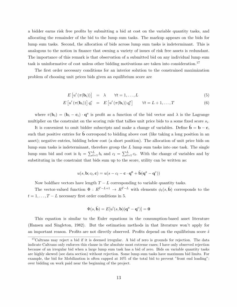
a bidder earns risk free profits by submitting a bid at cost on the variable quantity tasks, and

allocating the remainder of the bid to the lump sum tasks. The markup appears on the bids for

lump sum tasks. Second, the allocation of bids across lump sum tasks is indeterminant. This is

analogous to the notion in finance that owning a variety of issues of risk free assets is redundant.

The importance of this remark is that observation of a submitted bid on any individual lump sum

task is uninformative of cost unless other bidding motivations are taken into consideration.17

The first order necessary conditions for an interior solution to the constrained maximization

problem of choosing unit prices bids given an equilibrium score are

E[u′ (π(bi))

]= λ ∀t = 1, . . . , L (5)

E[u′ (π(bi))

]qet = E

[u′ (π(bi)) q

at

]∀t = L+ 1, . . . , T (6)

where π(bi) = (bi − ci) · qa is profit as a function of the bid vector and λ is the Lagrange

multiplier on the constraint on the scoring rule that tallies unit price bids to a some fixed score si.

It is convenient to omit bidder subscripts and make a change of variables. Define b = b − c,

such that positive entries for b correspond to bidding above cost (like taking a long position in an

asset); negative entries, bidding below cost (a short position). The allocation of unit price bids on

lump sum tasks is indeterminant, therefore group the L lump sum tasks into one task. The single

lump sum bid and cost is bl =∑L

t=1 bt and cl =∑L

t=1 ct. With the change of variables and by

substituting in the constraint that bids sum up to the score, utility can be written as:

u(s,b; cl, c) = u(s− cl − c · qe + b(qa − qe))

Now boldface vectors have length T − L corresponding to variable quantity tasks.

The vector-valued function Φ : RT−L+1 → RT−L with elements φt(s, b) corresponds to the

t = 1, . . . , T − L necessary first order conditions in 5.

Φ(s, b) = E[u′(s,b)(qa − qe)] = 0

This equation is similar to the Euler equations in the consumption-based asset literature

(Hansen and Singleton, 1982). But the estimation methods in that literature won’t apply for

an important reason. Profits are not directly observed. Profits depend on the equilibrium score s

17Caltrans may reject a bid if it is deemed irregular. A bid of zero is grounds for rejection. The dataindicate Caltrans only enforces this clause in the absolute most extreme cases; I have only observed rejectionbecause of an irregular bid when a large lump sum task has a bid of zero. Bids on variable quantity tasksare highly skewed (see data section) without rejection. Some lump sum tasks have maximum bid limits. Forexample, the bid for Mobilization is often capped at 10% of the total bid to prevent ”front end loading”:over bidding on work paid near the beginning of the project.

13

and unobservable costs that compose bidder types cl and c · qe.To further characterize equilibrium bidding and make the problem tractable for estimation, I

use an important result from the scoring auction literature (Asker and Cantillon, 2008; ?). With

constant absolute risk aversion the allocation of unit price bids on variable quantities tasks is

independent of types c · qe and the equilibrium choice of the score s. The Asker and Cantillon

(2008) result relies on quasi-linear preferences so their result doesn’t directly apply. But, constant

absolute risk aversion serves the same purpose as quasi-linear preferences in the sense that wealth

effects don’t affect the allocation problem. Proposition 2 in the appendix formally states the claim

and provides a proof.

An especially convenient feature of this result is that unit price bids do not depend on the

bidding behavior of rivals. Intuition of first price auctions suggests a unit price bid should include

a profit markup that depends on the competitiveness of the auction. Strategic interaction only

matters for the choice of the score and consequently, the lump sum component of the bid. Interest

centers on variable quantity tasks because I cannot measure incompleteness for lump sum task.

Therefore it is sufficient to only consider variable quantity tasks.18 Characterization (unreported)

of the first stage problem, choosing a score, follows the standard derivation for a first-price auction

with bidder types defined by a pseudo-type, ci · qe.

5 1st Order Taylor Series Expansion

After establishing the proposition I take a Taylor series approximation centered around bids at cost

b = 0 to approximate u′(π(b)). This expansion will provide guidance on how to form a basis for

the sieve estimator. Under constant absolute risk aversion (CARA) representation utility takes the

following form: u(x) = −1γ e−γx + k where k is a constant that normalizes a losing bidder’s payoff

to zero.

1st order

e−π(b)γ = e−π(0)γ − γe−π(0)γ(qa − qe)′b +R1 = T1 +R1

π(0) = s− cl − c · qe

18This lack of dependence on strategic interaction is an artifact of the CARA utility. A bidder withdecreasing absolute risk aversion skews more aggressively as wealth increases. In the model, wealth is higherfor larger values of si − ci · qe. This can be demonstrated by following the same derivation with constantrelative risk aversion—a representation with decreasing absolute risk aversion. In unreported work I performthe tests proposed in Athey and Levin (2001) and reject the hypothesis that bidders behave in accordancewith decreasing absolute risk aversion. I also reject the hypothesis that smaller contractors exhibit less riskaversion than larger contractors. I conclude a CARA representation is appropriate.

14

2nd order

e−π(b)γ = T1 − γ2e−π(0)γ(qa − qe)′b(qa − qe)′b +R2 = T2 +R2

Nth order

e−π(b)γ = TN−1 ± γNe−π(0)γ∏N

(qa − qe)′b +RN

For the moment suppose bids are assumed to be very close to cost, so that the remainder terms

in the Taylor series terms are zero. Plugging the expansions into the first order conditions I derive

the following moment conditions.

1st order

E[e−π(0)γ(qa − qe)− γe−π(0)γ(qa − qe)′b(qa − qe)] = 0

1

γE[(qa − qe)] = E[(qa − qe)(qa − qe)′]b

e−π(b)γ = e(s−cl−c·qe)γ=constant and cancels out inside expectation operator because it doesn’t

depend on qa. A convenient feature of the first order Taylor series expansion is that that the

expression is invertible.

bi = ci +1

γE[(qa − qe)(qa − qe)′

]−1(E[qa]− qe) (7)

The inversion admits a representation of bids that is linear in cost and terms that capture bid

skewing. To understand this equation, first consider the simple case with 1 variable quantity task

and 1 lump sum task. The unit price bidding equation is,

bit = cit +1

γ

E[qat ]− qetE[(qat − qet )2]

(8)

A unit price bid is a linear function of unit cost and a skewing term that depends on the

difference in a bidder’s expectation of the actual quantity and the engineer’s original quantity.

The comparative statics match the intuition presented in Gate’s (1959) example. If a bidder

expects quantity to overrun, it skews its bid above cost, and skews below cost if an underrun

is expected. Skewing aggressiveness increases for larger quantity differences. Risk considerations

temper skewing aggressiveness. The term in the denominator, γ, is the Arrow-Pratt measure of

absolute risk aversion; a more risk averse bidder skews less aggressively. The variance-like expression

E[(qat −qet )2] is the riskiness of a quantity change; bidders skew less aggressively if quantity changes

are expected to be more volatile. If a bidder forecasts no change and expects volatility, it would

submit a bid equal to cost.

15

With more than one variable quantity task, unit price bids are a linear function of unit cost and

a skewing term that involves an expression resembling the inverse of a covariance matrix of quantity

overruns. Not only does the expected overrun on a quantity affect the direction and aggressiveness

of a skew, skewing also depends on the covariances and expected overruns of other tasks. This is

analogous to the idea in finance that an optimal portfolio depends on the correlation of returns

across all assets. The engineering literature discusses how contractors, like modern investors, use

sophisticated computer algorithms that take into account the correlation structure of quantity

changes.19

The econometric procedure places restrictions on the covariance-like matrix E [(qa − qe)(qa − qe)′]

to construct a sieve basis of the form.

bi = ci +∑

att′(E[qa]− qe)

where the nuisance parameters att′ correspond to variance and covariance terms for task t with

t′ in the expression 1/γE [(qa − qe)(qa − qe)′]−1. The econometric section further discusses the

basis.

With a higher order expansion, it is not possible to invert, and the sieve method won’t work.

The above derivations are particularly convenient because of the linearity. To see the complication

consider the second order Taylor series expansion.

2nd order

0 = E[(qa − qe)]− γE[(qa − qe)(qa − qe)′]b +γ2

2E[(qa − qe)(qa − qe)′(qa − qe)]b′b

Notice I can’t invert to solve for b because it is a quadratic equation. An alternative estimator

to the sieve would be a moment based estimator where I directly measure the terms E[(qa−qe)(qa−qe)′] terms and E[(qa−qe)(qa−qe)′(qa−qe)]. In practice, the data do allow for direct estimation.

Perhaps more serious, measurement error is a major problem. Any measure of the terms inside

the expectation operator has measurement error. In the linear 1st order case, there are standard

instrumenting techniques to deal with measurement error. But measurement error solutions are

not so readily available in the highly non-linear cases.

The above derivation assumed negligible approximation error in the taylor series expansion.

For the 1st order expansion, Taylor’s theorem shows that there exists some bid x such that the

following exact equality holds in the FOC.

0 = E[e−π(0)γ(qa − qe)− γe−π(x)γ(qa − qe)(qa − qe)′]b

Then by inverting

19Cattell et al. (2007) reviews these methods.

16

bi = ci +1

γE

[u′(x)

u′(0)(qa − qe)(qa − qe)′

]−1

(E[qa]− qe)

If x is far from 0, the approximation in equation 7 may be far from the true value. In on-going

work, I am considering what conditions can be used to handle the approximation error.

6 Data and Descriptive Evidence

The data were collected from public records of construction projects procured by the California

Department of Transportation. The sample includes all 32 bridge projects bid on and built be-

tween 2002 and 2005 using the design-bid-build procurement method. Most of the variables from

the modeling section are found directly in the bidding documents. They list construction tasks,

engineer’s quantities, unit price bids, and a complete record of subcontracted tasks for all bidders.20 In addition, they contain identifying information for bidders (names, addresses, phone numbers),

and the names of, and tasks to be performed by, each subcontractor hired by a prime contractor.

Subcontracting information is available for all bidders, even those that lose the auction. In total

there are 17,018 observations of prime contractors’ “make or buy” decisions for individual work

items.

The sample includes 331 contractors. Of these, 74 participate as a prime contractor. In total

they submit 178 bids on the 32 projects. On average, a project receives 5.6 bids with a minimum of

2 and maximum of 13. 274 contractors participate as subcontractors. 17 contractors participate at

least once as a prime contractor and at least once as a subcontractor. The average project-bidder

subcontracts 37% of project work by value.

These are not monumental bridges. Engineers estimate a “fair and reasonable” cost. By this

measure, project range in size from $700,000 to $22,700,000 with an average of $7,000,000. For

comparison, the replacement 35W bridge is valued at $234 million and the new east span of the San

Francisco Oakland Bay Bridge into the billions of dollars. From visual inspection of Google Earth

satellite images21 I see the sample includes interstate overpasses, ramps and exchanges, and state

highway bridges spanning rivers, creeks, washes, and hillside ravines.22 For the average project

20To comply with the Subletting and Subcontracting Fair Practice Act, contractors name all subcontractorsthat perform more than 1/2% of the work.

21A bridge’s precise location was found by cross referencing location data in the bidding documents withinformation from the Federal Highway Administration’s National Bridge Inventory.

22Sample inclusion requires a project to use the task labeled “Structural Concrete, Bridge.” All bridges,even steel bridges, require concrete. Many projects let during this time period were sound walls wherea bridge member is built for a section of masonry wall. I only included bridges designed for vehiculartraffic. Also excluded are very large interstate construction projects with project values on the magnitudeof hundreds of millions of dollars into the billions.

17

there are 94 tasks; by comparison, Caltrans highway paving projects average 33 tasks.23 Bridges

require more tasks because a free standing structure is built in addition to some paving work that

all bridge projects require.

6.1 Construction Tasks

Across the 32 projects, there are 2,511 variable quantity and 482 lump sum project-tasks. Caltrans

classifies tasks using a coding system similar to NAIC industrial classifications. The sample includes

982 distinct tasks (indexed t). On average a task, t, is used on 3 of the 32 projects. Table 2 lists

26, Caltrans defined, categories of construction tasks at an aggregated level of grouping (hereafter

referred to as industries and indexed τ). The table also lists the dollar-valued amount of work

performed in each industry and the fraction of work subcontracted. Industry literature and primary

sources list the types of tasks that are considered ancillary and heavy construction tasks.24 Taking

this into account, I separate the industries into the two groups. I separate the industries because

prime contractors are heavy civil engineering construction firms, not ancillary task firms. This

assertion is evident in the data. A contractor only sells its services on the subcontract market if

it has capabilities in that task.25 Prime contractors have a 6% share of subcontracts for heavy

construction tasks, and there are only a few exceptions where a prime contractor serves as a

subcontractor on ancillary tasks.26 That an industry, such as “Reinforcement” (installing rebar),

is always subcontracted does not indicate prime contractors lack capabilities. Historic iron worker

union rules prohibit employment by a firm that hires any non-union workers on a particular project.

Thus a prime contractor must subcontract reinforcement. There are cases where a prime contractor

subcontracts reinforcement, yet serves as a subcontractor for a rival bidder.

Caltrans provides blue book prices for all standardized tasks in its California Cost Data Book.

This booklet is published annually. Blue book prices are based on unit price bids for all projects

awarded by Caltrans.

23Statistic from Bajari et al. (2007).24Sources include scholarly articles and books from the construction management literature (Arditi and

Chotibhongs, 2005; Hinze, 1993; Sweet, 2004). Primary sources include discussions with contractors onthe 35W bridge project and the annual investor report of Granite Construction, the only publicly tradedcompany in the sample. Caltrans’ documents do not separate heavy and ancillary tasks.

25Industry sources and practitioners cite that prime contractors do achieve a minimum efficient scale tomaintain divisions in ancillary tasks (Hinze, 1993; Sweet, 2004; Arditi and Chotibhongs, 2005). I define”having capabilities” to mean a firm achieves the minimum efficient scale.

26Modern Alloys, a large firm that installs metal beam guard rails and concrete barriers once participatedas a prime contractor. Granite Construction, the largest firm in the sample did a $300,000 subcontract forconcrete sidewalks. Twice a prime contractor performed clearing and grubbing, once removed a tree, andonce installed a small concrete barrier.

18

6.2 Incompleteness

Actual installed quantity data, qact, were collected from final payment forms, administered by Cal-

trans’ finance department. Incompleteness, incct is measured as deviations in installed quan-

tities from those specified in the original plans. It has a nested structure: overruns incct =∣∣∣ qact−qectqect

∣∣∣1(qact > qect), underruns incct =∣∣∣ qact−qectqect

∣∣∣1(qact ≤ qect), and the nested variant with no direc-

tional distinction incct =∣∣∣ qact−qectqect

∣∣∣. I only use variable quantity tasks. For lump sum tasks it is

not possible to quantify a task specific measure of incompleteness because, by definition, quantities

cannot vary. The main point from the prior discussion about incompleteness is that there is large

degree of variation (see table 1). Also note there is no systematic tendency for tasks to be perfectly

designed.27 There is large variation in the overall degree to which a project is completely specified.

Weighted by dollar value, the most completely designed project averages quantity deviations in

absolute value of just 1%; the most incomplete, 45%.

6.3 Prime Contractors and Subcontractors

The industry is localized for both subcontractors and prime contractors. The average prime con-

tractor enters bids on 2.4 of the 32 projects; the average subcontractor enters subcontracting

agreements on 2.5 projects. On projects for which a contractor participates, the average distance

between a firm’s nearest construction office and the job-site is 98 miles for prime contractors and

94 miles for subcontractors.28 Some of the contractors operate in the California wide market. This

generates skew in the size distribution of firms. I classify any bidder that enters bids on fewer than

4 projects as a “fringe” firm. Ten of the 74 prime contractors are classified as non-fringe. Studies

of highway procurement commonly make this distinction.29

Subcontractors are more specialized than prime contractors. The average subcontractor per-

forms work in 2 of the 26 industries; the average prime contractor, in 16. Finally, as anecdotal

evidence, 149 of the 274 (54%) subcontractors’ business names references a construction specialty

whereas only 5 of 74 for prime contractors. 30

27The concern is that tasks measured in discrete units, such as a stoplight where the original quantity is anumber like 4, would be perfectly designed whereas tasks measured in continuous units, such as cubic metersof concrete, would have at least a minor change. This is not the case.

28Construction office locations found by cross referencing address data from the bidding documents withaddress information provided by companies own websites, and Google maps “find business” directory. Ivisually verified that the address is a construction office and not equipment yard or private residence. Forcontractors with multiple offices, the nearest office is paired to a project.

29See Bajari et al. (2007), Krasnokutskaya (2009).30Examples of subcontractor specialty titles: Mike Brown Electric, West Coast Demolition, Pisor Fence.

Prime contractor specialty titles: Lees Paving, Security Paving, Parnum Paving, Modern Alloys, BencoBridges. Example non-specialty names: Shasta Constructors, Sterndahl Enterprises, Kiewit Pacific.

19

6.4 Unit Price Bids

The median bottom line bid, si is 5% above the engineer’s cost estimate and the standard deviation

of total bids divided by engineer estimates is 0.22. The moderate bid dispersion represents hetero-

geneity in bidders’ total costs (in the model, heterogeneity in pseudo-types ci · qe). The median

unit price bid, bcit, is 22% above the blue book value and the standard deviation is very large, 3.25.

The large bid dispersion cannot be fully attributed to cost heterogeneity. Bids are skewed.

6.5 Excluded Data

For estimation, lump sum tasks are excluded because incompleteness cannot be measured and the

bid need not reflect cost by the indeterminacy result. Non-standard tasks are excluded because they

do not fall into industry classifications and blue book costs are unavailable. These exclusions do not

pose problems. Many lump sum tasks are administrative duties or do not involve a construction

service (pollution permits, warranties, mobilization). Nonstandard tasks are customized items like

those labeled “drinking fountain”, “bat habitat”, “San Francisco manhole”. Exclusions shrink the

sample size from 17,018 observations to 12,354—7,114 ancillary tasks and 5,240 heavy construction

tasks.

Table 3 lists additional summary statistics. Tables 4 and 5 list summary statistics for all

variables used in estimation. The bid skewing variables will be constructed in the following section.

7 Estimation

The goal of estimation is to determine the effect of contractual incompleteness on unit cost for

both primecontracting and subcontracting. In this section I describe the parametrization of cost

functions. Then, I discuss the fixed effect identification strategy to account for self-selection bias. I

also introduce a source of endogeneity for incompleteness and discuss why the fixed effects control

for this source of endogeneity. Finally, I present the sieve technique to correct bid skewing.

7.1 Parametrization of Cost Functions

Rather than working directly with unit costs, that, across types of construction tasks, do not share

a common unit of measurement, I instead use a normalized measure of unit costs. To normalize

divide unit costs by a task’s blue book value. Normalization admits a natural interpretation of

bids and costs as deviations from blue book value. It also controls for some of the unobserved cost

heterogeneity across types of tasks.

Observations are indexed by project c, bidder i, and task t. Let c∗cits and c∗citp be the (normalized)

unit cost of subcontracting and primecontracting and c∗cit be the cost of the chosen arrangement.

20

According to the subcontracting decision rule, prime contractors choose the lowest cost alternative.

Thus,

subcit =

{1 if c∗cits < c∗citp

0 if c∗cits ≥ c∗citpwhere the variable subcit indicates whether or not subcontracting is observed. The asterisks on

primecontracting and subcontracting cost variables emphasize that neither cost is directly observed

by the econometrician (they are both known to the bidder). Instead, bids of the chosen arrangement

are observed.

I specify cost functions linearly:

c∗citp = x′citpβ0p + βinc0p incct + ecitp (9)

c∗cits = x′citsβ0s + βinc0s incct + ecits (10)

The main variable of interest is contractual incompleteness, incct. The other covariates are

xcit; ecits and ecitp are error terms. The parameters, β0s and β0p capture marginal effects on

subcontracting and primecontracting costs, respectively. Both βinc0p and βinc0s are expected to be

positive. The differential effect, βinc0s − βinc0p , is relevant to test whether the variable affects the

make-or-buy decision.

Other covariates include the log of the distance between the job-site and the prime contrac-

tor’s nearest construction office and an indicator variable for whether the prime contractor is a

fringe firm. Distant prime contractors—infrequent participants in the local market, unfamiliar

with local ordinances, and facing higher costs to transport their own equipment — are predicted

to have higher primecontracting costs. For reputation reasons, distant contractors are predicted

to have higher subcontracting costs. Overall, its ambiguous how distance affects the relative costs

of subcontracting and primecontracting. For scale economies reasons, non-fringe contractors may

have large enough logs of work to warrant maintaining divisions in a broad scope of construction

activities. Thus fringe firms are predicted to have higher costs for primecontracting. This margin

may be particularly relevant for ancillary tasks. Fringe status also captures reputation factors for

both subcontracting and primecontracting.

Industry sources indicate project-task scale economies are an important determinant of unit

cost. They arise by spreading out project-task fixed costs across more work and because of learning-

by-doing. I include a normalized measure of the quantity:qectqet

. The denominator is the sample

average engineer’s original quantity for task, t.

21

7.2 Self-Selection Bias and Endogeneity of Contractual Incom-

pleteness

For the moment, suppose unit price bids equal unit cost. There is a potential self-selection bias

in OLS estimation of the separate cost equations. Inconsistency arises if an omitted variable has

a different effect on subcontracting costs and primecontracting costs. There is also the potential

for inconsistency due to the endogeneity of contractual incompleteness. The identification strat-

egy exploits the panel data structure to control for both self-selection bias and incompleteness

endogeneity.

The specifications include individual effects to capture industry, contract, and bidder specific

characteristics. Expand the composite error term:31

ecitp = ατp + αcp + αip + εcitp

ecits = ατs + αcs + αis + εcits

The individual effects ατs and ατp capture factors specific to industries 32 for both primecontracting

and subcontracting; the terms αcs and αcp, factors specific to the project; and αis and αip bidder

specific factors. Individual effects are allowed to be fixed: correlated with regressors. They can be

represented by dummy variables. Define zcits = [xcit, ατs, αcs, αis] and zcitp = [xcit, ατp, αcp, αip].

With dozens to hundreds of observations in each cluster, dummy variable estimation will not be

inconsistent due to an incidental parameters problem.

The residual error terms , εcits and εcitp, are assumed to capture exogenous cost shocks that

are common across primecontracting and subcontracting. They represent idiosyncratic input cost

shocks incurred by any subcontractor or prime contractor on a project-task (i.e. labor wages,

equipment rental rates, material costs).33 They also represents a bidder’s private information

about managerial and oversight costs. Formally, conditional on the fixed effect dummies, observed

covariates, and subcontracting choices,

E[εcits − εcitp|zcitp, zcits, subcit = 1] = 0

E[εcitp − εcits|zcitp, zcits, subcit = 0] = 0.

31Negative costs are in the support of the distribution because the specifications is in levels. The alter-native, taking the logarithm of unit costs, is an unattractive specification. Doing so, without the blue booknormalization, requires an individual effect for each type of task. This creates an incidental parametersproblem. Moreover, when I introduce bids, the bid skewing equation 7 is characterized in levels, not logs.

32τ subscripts refer to industry clusters, distinct from the t subscripts referencing tasks. See table 2 forthe list of industries.

33This generates correlation in cost shocks across observations within a project-task cluster. I clusterstandard errors by project-task.

22

The use of fixed effects for identification requires justification. In general, fixed effect speci-

fications are attractive because they control for a lot of the unobserved heterogeneity. I will not

attempt to exhaustively list all omitted variables that could generate self-selection bias. Instead I

will discuss a few that are important to the construction industry and other margins of the incom-

plete contracting theories of the firm besides the complexity and incompleteness in the contracting

environment.

Both the property rights and transaction costs theory predict asset characteristics are an im-

portant determinant of subcontracting decisions: examples include whether performance of a task

is complementary to the management activities of a prime contractor and whether equipment is

specific to the task. Industry fixed effects control for asset characteristics. I also consider agency

(Holmstrom and Milgrom, 1991), and relational contracting (Baker et al., 2002) theories of the

firm. Agency theory regards the importance of monitoring employees. For some tasks, such as

drilling, the care and maintenance of equipment requires attentive monitoring. Project fixed effects

also capture the importance monitoring. Monitoring is important for projects with limited con-

struction zone accessibility.34 Bidder fixed effects and fringe status capture the reputation status of

prime contractors. Industry fixed effects also capture institutional features such as the labor union

provisions for iron workers (discussed in the data section).

Endogeneity of contractual incompleteness (correlation between cost shocks and the incom-

pleteness measure) is a concern for two reasons. The first regards the job-site environment; the

second, quality and workmanship standards. Some job-sites, such as a mountainous ravine, present

significant engineering challenges. Such an environment would increase the cost of construction and

make it more costly to write a complete design. Projects with high unobserved quality standards

are costly and modifications exacerbate hold-up problems. As such, engineers find it worthwhile

to write more complete plans and specifications on high quality projects. The industry’s typical

example of a high quality, highly complete design, is an airport paving project. Contract fixed

effects control for unobserved quality standards and the job-site environment.

In the robustness section, I consider the Heckman (1979) control function approach as an

alternative identification strategy.

7.3 Sieve Bid-skewing Estimator

In this section I describe the sieve technique to correct bid skewing.

The inverted unit price bidding equation with all contract-task engineer quantities normalized

to one,

34On the 35W bridge separate contractors performed work on the north and south end of the bridge.Contractors could not monitor both ends of the bridge because the alternative river crossings were cloggedwith traffic. A bridge in my sample was along a mountain pass where materials and contractors came fromdistant towns on opposite ends of the pass.

23

bci = cci +1

γE[(qac − 1)(qac − 1)′

]−1(E[qac ]− 1)

is an additive function of unit cost and a skew term. To derive a tractable form for the sieves,

I place three restrictions on the covariance-like expression to exploit its symmetry. Rename the

matrix Vc := γE [(qac − 1)(qac − 1)′] with the i, j cell denoted as vcij . The superscript c references

the project.

Diagonal elements capture the variance of task overruns. The first restriction assumes tasks

within an industry, τ (i.e. roadwork, bridgework, ancillary tasks) share a common variance.

Restriction 1 vcii := vcτ for all i ∈ τ

Off diagonal terms capture covariances in task overruns. The second restriction assumes pair-

wise task covariances within industries and across industries are the same no matter which task

pair is considered.

Restriction 2 vcij := vcττ ′ for any i ∈ τ and j ∈ τ ′ and (i 6= j)

Risk of quantity changes varies across projects. Recall the average deviation of quantities across

tasks is 45% for the riskiest project and just 1% for the least risky. The third restriction preserves

the relative variances and covariances of industries and scales these values by a project’s overall

quantity change risk. Let the scalar ηc represent the quantity change risk for project c.

Restriction 3 ηcV = Vc

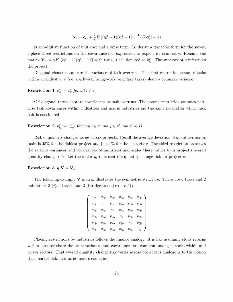
The following example V matrix illustrates the symmetric structure. There are 6 tasks and 2

industries: 3 (r)oad tasks and 3 (b)ridge tasks (τ ∈ {r, b}).

vr vrr vrr vrb vrb vrb

vrr vr vrr vrb vrb vrb

vrr vrr vr vrb vrb vrb

vrb vrb vrb vb vbb vbb

vrb vrb vrb vbb vb vbb

vrb vrb vrb vbb vbb vb

Placing restrictions by industries follows the finance analogy. It is like assuming stock returns

within a sector share the same variance, and covariances are common amongst stocks within and

across sectors. That overall quantity change risk varies across projects is analogous to the notion

that market riskiness varies across countries.

24

In the context of construction, these restrictions are reasonable. Events can have an effect that

ripple across tasks. For example, an event could increase the length of road by 10% which would

require a 10% increase in roadwork quantities. For another example, consider the modification to

the 35W bridge. When the piers were moved 20 feet, extra concrete, drilling and steel reinforcements

were needed to bear the additional load of a longer span.

Inversion preserves symmetry. With A := V−1, the unit price bidding equation becomes,

bci = c∗ci + 1ηcAE[(qac − 1)]. Expanding around some contract-task ct in industry τ provides a map

between a unit price bid and unit cost:

bcit = c∗cit +1

ηc

aτ (E[qact − 1]) +∑τ ′

aττ ′ ∑ct′∈τ ′∪c ct′ 6=ct

(E[qact′ − 1])

+ ψcit (11)

The diagonal coefficients, aτ , and off diagonal coefficients, aττ ′ (as a collection a) are the parame-

ters that are estimated in the sieves. The quantities inside the summation∑

ct′∈τ ′∪c ct′ 6=ct(E[qact′−1])

form the basis for the sieves. Actual quantities, qact serve as a measure for expected actual quan-

tities, E[qact]. Rather than estimating contract riskiness terms from bid data, I use the average

squared quantity changes on a project, 1Tc

(qac − 1)′(qac − 1), as an estimate of project riskiness, ηc.

The error term, ψcit, represents expectational error and idiosyncratic variations in bid skewing.

The most dense representation of the estimator would have one task within task category, but

it could not be estimated because there are too many nuisance terms T 2. A rank condition would

be violated. For estimation I consider a sieve with 3 industries: roadwork, bridgework and ancillary

tasks. There are a total of 9 sieve basis. In on-going work I am verifying the asymptotic properties

of the estimator to determine if it would have normal asymptotics or slower that root-n asymptotics.35

The specification is a system of four cost equations: on the subsamples of primecontracted and

subcontracted tasks for both heavy industries and ancillary tasks. Cross equation restrictions are

placed on the 9 covariates related to bid skewing.

Measurement error presents a limitation. There is expectational error in the incompleteness

variable and the bid-skewing variables.36 I consider the implications of measurement error while

interpreting results and further discuss in the robustness section. In on-going work, I consider an

instrumenting strategy that uses data in the bidders current information set I that can be used to

predict the direction and magnitude of quantity changes E[q−qe]. The instrument uses differences

35Alternatively the covariance structure could have been estimated from quantity data. This createsadditional non-linear measurement error because it is multiplied with the measurement already present inthe overrun term. As a robustness check I consider nested variants of the restrictions.

36Variables in a bidder’s current information set could serve as valid instruments for expectational error.Hansen and Singleton (1982) used lagged assets returns as instruments. Using the analog of their instruments,lagged quantity overruns, does not work because overruns are not correlated across projects located ingeographically distinct locations.

25

in original quantities for similar tasks. For similar tasks t and t′, I use qet − qet′ to instrument for

qat − qet . Consider a very simple example of nuts and bolts. Suppose the number of nuts must equal

the number of bolts. If the original quantity of nuts is higher than the original quantity of bolts,

contractor would expect bolt quantities to overrun. It may be possible to find examples on bridge

components where the nut-bolt example would apply.

8 Results

I first present the results on contractual incompleteness. I separately discuss heavy industries and

ancillary tasks. Next, I consider the other covariates (fringe status, distance, and scale economies).

Then, I present the results on bid skewing and discuss the bias from misspecification.

8.1 Heavy Industry Contractual Incompleteness

Table 6 reports the estimates for the most preferred specification. Notice that I restrict the coeffi-

cients on contractual incompleteness to be the same for overruns and underruns on primecontracted

work. In the unrestricted specification, the coefficients are not statistically different from one an-

other. Later, I discuss the econometric reasons for preferring the restricted specification in light of

measurement error and bid skewing.

First consider heavy industries. (refer to the bold-face estimates in table 6 under the columns for

heavy industries). Contractual incompleteness on overruns has a significant effect on subcontracting

costs. Interpreted as a dollar-valued elasticity, a 10 percentage point increase in quantity deviation

leads to a 4.5 percentage point increase in unit cost relative to the blue book value. In the range

from perfect design (no measured incompleteness) to overruns of 35%, subcontracting costs increase

about 12 percentage points. The range roughly corresponds to a movement from the 35 percentile

to the 80 percentile of the incompleteness variable. In contrast, contractual incompleteness from

underruns has zero effect on subcontracting costs. Thus, hold-up costs exist and are economically

large for subcontracting, but only in cases where contractors likely expect overruns. In contrast to

subcontracting, incompleteness has no effect on primecontracting costs. This is evidence that hold-

up costs are mitigated if heavy construction work is performed in-house by the primary contractor.

The distinction between overruns and underruns can indicate the type of hold-up that is oc-

curring. A leading source of dispute regards scheduling and acceleration (working overtime and

mobilizing additional workers and equipment). Quantity overruns are likely to trigger this sort of

ex-post haggling. In addition, ex-ante relationship specific commitments to pre-coordinate sched-

ules on the part of subcontractors and prime contractors could reap large benefits. The threat

of overruns and renegotiating schedules could reduce the amount of coordination. I focus this in-

terpretation on heavy construction tasks because they are the ones typically included in schedule

26

planning; ancillary tasks, which typically occur towards the end of a project, are excluded.37 Un-

derruns, which reduce the amount of work, alleviate scheduling pressures. In part, this explains

why underrun contractual incompleteness has no impact on subcontracting costs.

8.2 Ancillary Task Contractual Incompleteness

The results are quite different for ancillary tasks. First consider subcontracting (refer the bold-

faced entries under ancillary tasks in table 6). For underruns, contractual incompleteness has no

effect on subcontracting costs. Yet for overruns there is a very large impact on subcontracting

costs. In the range from perfect design to underruns of 35%, subcontracting costs increase about

23 percentage points. Scheduling hold-up does not seem to be important for ancillary tasks. Again,

scheduling is not expected to be important because, as tasks performed at the end, up to two years

after bidding, they are excluded from the pre-planning of schedules.

There is an explanation for the large hold-up stemming from underruns. Industry sources

state that quantity underruns cause disputes about lost revenue (Sweet, 2004). Subcontractors lose

business and cannot recoup project specific fixed costs. This hold-up is best interpreted in light of

the reference point theory (Hart and Moore, 2008). In the norm, subcontractors expect to cover

fixed costs. This is in spite of the terms of their original pricing contracts that adjust payment

based on quantities. The norm serves as their threat point for holding-up prime contractors.

Next consider primecontracting of ancillary tasks. Contractual incompleteness has a large

effect on primecontracting costs. In the previously discussed range, costs increase 15 percentage

points. At first glance, this result seems at odds with the theory of the firm; performing work

in-house typically decreases the hazards of contractual incompleteness. But, in fact, the theory

accommodates this result. As touched on earlier, prime contractors are heavy civil engineering

firms, not ancillary task firms.38 They do not maintain divisions in ancillary tasks because they

do not achieve an efficient scale. As such, when they elect to perform these tasks themselves, they

must engage in one-shot transactions with suppliers. The evidence points to severe contractual hold-

up. Specialized ancillary task subcontractors, operating in local markets, have frequent, repeated

interactions with local suppliers. The repeated transacting mitigates hold-up problems according

to relational contracting theories of the firm (Baker et al., 2002). The distinction is not present for

heavy construction tasks because both prime contractors and subcontractors are heavy construction

firms.

There is a tentative explanation for why underruns cause payment disputes for ancillary tasks

but not heavy construction tasks. It regards a government program about subcontracting to Disad-

37Contractors use a computerized system called the critical path method to schedule construction. Asnoted by Levin (1998) ancillary tasks are omitted.

38Industry practitioners and sources make this point, and I provide evidence in the data section to supportthis claim.

27

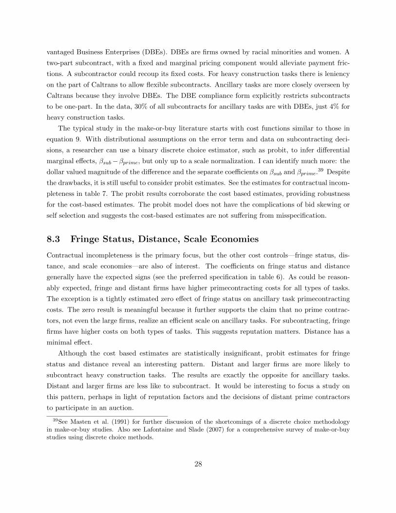
vantaged Business Enterprises (DBEs). DBEs are firms owned by racial minorities and women. A

two-part subcontract, with a fixed and marginal pricing component would alleviate payment fric-

tions. A subcontractor could recoup its fixed costs. For heavy construction tasks there is leniency

on the part of Caltrans to allow flexible subcontracts. Ancillary tasks are more closely overseen by

Caltrans because they involve DBEs. The DBE compliance form explicitly restricts subcontracts

to be one-part. In the data, 30% of all subcontracts for ancillary tasks are with DBEs, just 4% for

heavy construction tasks.

The typical study in the make-or-buy literature starts with cost functions similar to those in

equation 9. With distributional assumptions on the error term and data on subcontracting deci-

sions, a researcher can use a binary discrete choice estimator, such as probit, to infer differential

marginal effects, βsub−βprime, but only up to a scale normalization. I can identify much more: the

dollar valued magnitude of the difference and the separate coefficients on βsub and βprime.39 Despite

the drawbacks, it is still useful to consider probit estimates. See the estimates for contractual incom-

pleteness in table 7. The probit results corroborate the cost based estimates, providing robustness

for the cost-based estimates. The probit model does not have the complications of bid skewing or

self selection and suggests the cost-based estimates are not suffering from misspecification.

8.3 Fringe Status, Distance, Scale Economies

Contractual incompleteness is the primary focus, but the other cost controls—fringe status, dis-

tance, and scale economies—are also of interest. The coefficients on fringe status and distance

generally have the expected signs (see the preferred specification in table 6). As could be reason-

ably expected, fringe and distant firms have higher primecontracting costs for all types of tasks.

The exception is a tightly estimated zero effect of fringe status on ancillary task primecontracting

costs. The zero result is meaningful because it further supports the claim that no prime contrac-

tors, not even the large firms, realize an efficient scale on ancillary tasks. For subcontracting, fringe

firms have higher costs on both types of tasks. This suggests reputation matters. Distance has a

minimal effect.

Although the cost based estimates are statistically insignificant, probit estimates for fringe

status and distance reveal an interesting pattern. Distant and larger firms are more likely to

subcontract heavy construction tasks. The results are exactly the opposite for ancillary tasks.

Distant and larger firms are less like to subcontract. It would be interesting to focus a study on

this pattern, perhaps in light of reputation factors and the decisions of distant prime contractors

to participate in an auction.

39See Masten et al. (1991) for further discussion of the shortcomings of a discrete choice methodologyin make-or-buy studies. Also see Lafontaine and Slade (2007) for a comprehensive survey of make-or-buystudies using discrete choice methods.

28

Task economies of scale are significant, and explain more variation in unit price bids than any

other regressor (see table 6). It is notable that scale economies are larger in magnitude for primecon-

tracting. Learning-by-doing is important on the job site and could possibly explain the difference.

Subcontractors experience less learning-by-doing on any given project because they typically work

on many more projects in a construction season than prime contractors. The difference in scale

economies suggests prime contractors close the learning gap with more work.

8.4 Bid Skewing

A lot of care has been put into bid skewing. First consider the raw estimates on the bid-skew

parameters. The top panel of table 8 presents estimates of the 9 bid-skew parameters for the

preferred specification. The diagonal terms are positive for all three industries. As expected, this

indicates bidders skew up on overruns and down on underruns. The bottom panel reports point

estimates of the variance matrix V—the calculated inverse of the estimates for A.

For ancillary tasks, the diagonal term in A is small relative to bridge and road tasks. This

implies the expected variance in quantity changes are high (see corresponding diagonal term in

V), and hence, risk averse bidders do not skew aggressively on ancillary tasks. The covariances

amongst ancillary tasks, and with road and bridge tasks are small in comparison to the variance.

The diagonal terms in A are large for road and bridge tasks. This implies the expected variance

is small, and hence, bidders skew more aggressively on these tasks. For a sense the magnitude,

the predicted skew is 12.6% above cost for a one standard deviation overrun on a bridge task if

the covariance terms are ignored.40 The covariances amongst and across road and bridge tasks are

significant, which indicates that bidders do in fact make sophisticated portfolio allocation decisions.

8.5 Auction Design to Eliminate Bid Skewing

The estimated results on bid skewing verify contractors are indeed skewing, and moreover skewing

in a predictable manner. An improvement to the auction design would be for the department of

transportation to score the auctions using E[qat ] rather than qet . Under this alternative scoring

mechanism, it’s straightforward to verify in the first order conditions that bidder’s would submit

a bid of bt = ct for all variable quantity tasks. For the department of transportation to implement

this scoring rule, it would require them to scrutinize projects in the same way contractors do to

form bidding strategies. The engineer’s certainly have the necessary knowledge and experience to

do so. Even if they couldn’t fully eliminate skewing incentives they could at least implement a

scoring rule that more closely aligns with expected actual quantities.

40A one standard deviation change in the diagonal bid-skew variable for bridge tasks is 1.423 (see table5).

29

In on-going work, I use estimates c of unit price costs and calculate the auction outcome

under the counterfactual that the scoring rules uses E[qat ]. Intuitively, the DOT is better off

because contractors are not profiting from skewing, and bidder’s are better off because they face no-

uncertainty and won’t build in a risk premium into their bottom line bid. Note in the counterfactual

that I cannot estimate the score s that would be submitted under the new scoring rule. It would

be higher because bidders aren’t profiting on skewing, but net the increase in the score would be

dampened by having a lower risk premium.

8.6 Bid-Skewing Bias

I need to account for bid skewing to avoid bias in the contractual incompleteness estimates on sub-

contracting. Table 10 illustrates the bias from misspecification. The table shows three specifications

ordered from the most biased specification, with no bid-skew correction terms and no restrictions

on the contractual incompleteness variable, to a moderately biased specification with the bid-skew

correction and unrestricted coefficients, to the most preferred specification. The arrows indicate

the direction of bias on the contractual incompleteness estimates relative to the preferred specifi-

cation. First consider the differences between the most biased estimates and the moderately biased

estimates. This source of bias is easy to interpret. Recall the basic intuition about bid-skewing;

bidders skew up on overruns and down on underruns. Without the bid skew correction, the over-

run contractual incompleteness estimate is larger because the estimated coefficient is picking up

the effect of bidders skewing up, and the underrun incompleteness is smaller because it is picking

up downward skewing.

The bias in the moderately biased, unrestricted specification relative to the preferred, restricted

specification, again, boils down to a failure to fully account for bid skewing. The source of this failure

is subtle. It is caused by contamination bias from measurement error. Classical measurement error,

in a simple econometric model with a single regressor that is orthogonal to the other regressors only

causes attenuation bias. This econometric model is more complicated. There is measurement error

in two types of variables: the contractual incompleteness variables and the bid-skew variables.41

Moreover, these variables are highly correlated; the bid-skew terms are positively correlated with

overrun incompleteness and negatively correlated with underrun incompleteness. The correlation

creates contamination bias. By placing the restrictions on primecontracting incompleteness, I am

using an incompleteness variable∣∣∣ qact−qectqect

∣∣∣ that is less correlated with the bid-skew terms. To see

how the restrictions effect the estimated bid-skew terms, compare the diagonal elements in A

from the preferred, restricted specification (table 8) to those in the unrestricted specification (table

9). The diagonal terms are smaller in the unrestricted specification. Essentially, the unrestricted

model underestimates the degree of bid skewing which, in turn, biases the estimates on contractual

41In the unrestricted specification, there are 8 contractual incompleteness variables and 9 bid skew terms.

30

incompleteness.

The magnitude of the bias is large. Across the 8 incompleteness categories, a quick calculation

shows the coefficients in the worst specification are biased by at least 17% and up to a factor of 8.

I calculate the bias as∣∣∣βpref−βbiasedβpref

∣∣∣. For underruns on heavy industries, the bias is so great that

the coefficient signs change to negative values.

9 Robustness

The identification strategy relies on fixed effects to control for selection. An alternative specification

considers a switching regression technique that uses a control function approach (Heckman, 1979).

In the Roy (1951) model framework, where selection is based solely on cost outcomes and not on

non-monetary considerations, finding valid exclusion restrictions is challenging. This is especially

challenging because the excluded variables should be at the detailed level of a project-task.42

I tested a specification without exclusion restrictions. The estimates differ negligibly, and the

coefficients on the control functions are statistically insignificant which is not surprising given the

fixed effects already control for the key unobserved variables.

I also consider a specification that relaxes the Roy (1951) model framework where I do have a

justifiable exclusion restriction. The exclusion restriction is based on two regulations: the require-

ment to make a “good faith effort” to hire disadvantaged business enterprise (DBE) subcontractors

and subcontracting limits. The DBE requirement (stated as a percentage of total contract value)

could be a plausible exogenous shifter of subcontracting probabilities that has no effect on either

subcontracting or primecontracting costs. In the data, a higher DBE goal increases the amount of

ancillary tasks subcontracted, and when the cap bids, there is a reduction in the amount of heavy

construction tasks subcontracted. The data show DBE’s almost exclusively perform ancillary tasks

(30% of all ancillary task subcontracts and 4% of heavy construction subcontracts). The DBE

subcontractors’ specialty in ancillary task explains the positive correlation between subcontracting

probabilities and the DBE goal. The binding cap explains the negative correlation for heavy con-

struction tasks. Estimates preserve results, but magnitudes differ. There is an important tradeoff

in using this method. I must drop project fixed effects which is why I find this an undesirable

specification.

Unit price bids display an extreme amount of dispersion. Beeston (1975) first documented this

fact, and I find it in this data. For example, within the same project-task the highest bid is on

average 7.49 times greater than the lowest. In situations when the same subcontractor is hired for

a project-task—presumably costs are nearly identical—this ratio is 3.49. Other measures of bid

42To identify subcontracting costs the excluded variables should affect primecontracting costs and notsubcontracting costs. To identify primecontracting costs the excluded variables should affect subcontractingcosts and not primecontracting costs.

31

dispersion show the same pattern. This dispersion cannot be reconciled by heterogeneity in cost

or risk aversion. There are 4 possible explanations. First, pairwise task correlation could be quite

high in which case those tasks are skewed as a pair rather than individually. Allocation within

the pair is arbitrary. Second, if bidders do not expect volatility in quantity, the task resembles a

lump sum task. Third, with an average of 94 tasks, where quantities average out to zero overrun,

there is little aggregate risk to arbitrarily allocating unit price bids. Fourth, industry sources state

that contractors have an incentive to conceal their true unit costs from Caltrans and rivals by

randomizing bids. The econometric technique corrects for systematic bid skewing, but it cannot

fully control for the full amount of bid dispersion. As a result, bid dispersion adversely impacts

estimation efficiency. This fact is actually reassuring because the relatively large standard errors are

primarily an artifact of bid dispersion, not an indication that the effects of interest are insignificant.

10 Conclusion

This paper provides empirical evidence that complexity and incompleteness in contracting environ-

ments has a substantial impact on costs in the construction industry. As the incomplete contracting

theories of the firm predict, the effect differs for primecontracting (in-house) and subcontracting

(market) transactions. Unlike traditional studies of the “make or buy” decision that provide quali-

tative evidence about firm boundaries, this study quantifies the dollar-valued cost of those decisions.

Such a research design is made possible because contractors’ bids, after correcting for bid skewing

strategies, reflect cost.

I developed a model of the subcontracting and competitive bidding process for Caltrans bridge

projects. At the detailed level of a work item, prime contractors submit a unit price bid and

decide whether to perform work themselves or hire a subcontractor. I proposed a measure of

incompleteness—the difference in original and revised work item quantities. I characterized bidding

behavior which shows how bidders forecast quantity changes to allocate unit price bids based on

principles analogous to those in modern portfolio theory. Finally, I embed this characterization into

the econometric procedure to get an unbiased estimate of how contractual incompleteness affects

both subcontracting and primecontracting costs.

The results show that incompleteness not only matters, but also has a big economic impact on

firm boundaries. For heavy construction tasks, subcontracting involves significant hold-up costs,

particularly when scheduling pressures matter. Performing in-house mitigates these costs. For

ancillary tasks, incompleteness impacts cost under both forms of organization. The effect for

subcontracting is modest, except one case. In anticipation of quantity underruns, there are severe

frictions likely stemming from disputes about lost revenue. The effect for primecontracting is quite

large. Relational theories of the firm accommodate this seemingly contradictory result. Heavy civil

32

engineering prime contractors transact with ancillary task suppliers on a one-shot basis. In contrast,

specialty subcontractors mitigate supplier hold-up because of frequent, repeated transacting.

This paper also provides a glimpse of evidence about relational determinants of firm boundaries

by considering the fringe status of contractors and their proximity to the job-site. Reputation factors

appear to differ for heavy and ancillary tasks. There is interest in further studies of relational

contracting in this industry.43

In conclusion, I offer practical thoughts on procurement practices and motivate policy relevant

research. Public agencies are typically concerned about the competitiveness of the procurement

process. As such, they try to promote competition with the goal of reducing bidder markups.

Markups are already small, estimated in other papers to be around 4% in highway contracts.44

This suggests there are negligible gains available from promoting further competition. This paper

suggests an alternative, and perhaps, more effective means to achieve cost savings. As part of a

cost-benefit analysis, the most stark prescription would be for engineers to prepare more complete

plans and for buyers to avoid making ex-post changes. As a qualification, I can only comment on

the benefit of writing more complete plans, not the cost.

Using the nuanced results on overruns and underruns, and heavy construction and ancillary

tasks I can offer more directed thoughts. For example, on heavy construction tasks, avoid making

changes that generate scheduling pressures. On ancillary tasks, interacting this paper’s results

with a more detailed analysis of the Subcontracting and Subletting Fair Practice Act, could uncover

opportunities for additional cost savings. The act requires prime contractors to name all subcon-

tractors in the pre-bidding phase, as opposed to the time of construction when plans could be more

complete. There is also scope to explore how subcontracting limits and minority subcontracting

requirements distort subcontracting decisions, and how those distortions interact with the results

on contractual incompleteness.

Construction is particularly important in times of economic slowdown. It is a leading tool of

fiscal stimulus. Recently, there has been a lot of publicity about shovel-ready projects. Contractual

incompleteness and the associated wasteful costs would be modest. But, since fiscal policy needs to

act quickly, the next round of fast-tracked projects are prone to be quite incomplete. With this in

mind, policy makers should think about how many highways and bridges they can buy with their

stimulus dollars.

43An example is Gil and Marion (2009).44Estimate taken from Bajari et al. (2007). Their survey of the literature finds similar markups.

33

References

D. Acemoglu, P. Aghion, R. Griffith, and F. Zilibotti. Vertical Integration and Technology: Theory

and Evidence. Journal of European Economic Association(forthcoming), 2009.

D. Arditi and R. Chotibhongs. Issues in Subcontracting Practice. Journal of Construction Engi-

neering and Management, 131(8):866–878, 2005.

J. Asker and E. Cantillon. Properties of Scoring Auctions. RAND Journal of Economics, 39(1):

69–85, 2008.

S. Athey and J. Levin. Information and Competition in US Forest Service Timber Auctions. Journal

of Political Economy, 109(2), 2001.

P. Bajari and G. Lewis. Procurement Contracting with Time Incentives: Theory and Evidence.

University of Minnesota and Harvard, mimeo, 2008.

P. Bajari and S. Tadelis. Incentives versus Transaction Costs: A Theory of Procurement Contracts.

The RAND Journal of Economics, 32(3):387–407, 2001.

P. Bajari, S. Houghton, and S. Tadelis. Bidding for Incomplete Contracts: An Empirical Analysis.

University of Minnesota: mimeo, 2007.

G. Baker and T. Hubbard. Contractibility And Asset Ownership: On-Board Computers and

Governance In US Trucking. Quarterly Journal of Economics, 119(4):1443–1479, 2004.

G. Baker, R. Gibbons, and K. Murphy. Relational Contracts and the Theory of the Firm. Quarterly

Journal of Economics, 117(1):39–84, 2002.

D. Beeston. One Statistician’s View of Estimating. Chartered Surveyor, Building and Quantity

Surveying Quarterly, 2(4), 1975.

S. Campo, E. Guerre, I. Perrigne, and Q. Vuong. Semiparametric Estimation of First-Price Auctions

with Risk Averse Bidders. 2003.

D. Cattell, P. Bowen, and A. Kaka. Review of Unbalanced Bidding Models in Construction. Journal

of Construction Engineering and Management, 133:562–573, 2007.

F. Ciliberto. Does Organizational Form Affect Investment Decisions? The Journal of Industrial

Economics, 54(1):63–93, 2006.

R. Coase. The Nature of the Firm. Economica, 4(16):386–405, 1937.

34

D. De Silva, T. Dunne, A. Kankanamge, and G. Kosmopoulou. The Impact of Public Information

on Bidding in Highway Procurement Auctions. European Economic Review, 52(1):150–181, 2008.

S. Forbes and M. Lederman. Does Vertical Integration Affect Firm Performance? Evidence from

the Airline Industry. University of Toronto, mimeo, 2008.

S. Forbes and M. Lederman. Adaptation and Vertical Integration in the Airline Industry. American

Economic Review (forthcoming), 2009.

M. Gates. Aspects of Competitive Bidding. Annual Report of Connecticut Society of Engineers,

1959.

R. Gil. Make-or-buy in movies: Integration and ex-post renegotiation. International Journal of

Industrial Organization, 25(4):643–655, 2007.

R. Gil. Revenue Sharing Distortions and Vertical Integration in the Movie Industry. Journal of

Law, Economics, and Organization(forthcoming), 2008.

R. Gil and J. Marion. The Role of Repeated Interactions, Informal Agreements and Relational

[Sub]Contracting: Evidence from California Highway Procurement Auctions. UCSB: mimeo,

2009.

S. Grossman and O. Hart. The Costs and Benefits of Ownership: A Theory of Vertical and Lateral

Integration. The Journal of Political Economy, 94(4):691, 1986.

L. Hansen and K. Singleton. Generalized Instrumental Variables Estimation of Nonlinear Rational

Expectations Models. Econometrica, 50(5):1269–1286, 1982.

G. Harrison and E. Rutstrom. Risk Aversion in the Laboratory. Risk Aversion in Experiments,

2008.

O. Hart and J. Moore. Property Rights and the Nature of the Firm. Journal of Political Economy,

98(6):1119, 1990.

O. Hart and J. Moore. Contracts as Reference Points. Quarterly Journal of Economics, 123(1):

1–48, 2008.

J. Heckman. Sample Selection Bias as a Specification Error. Econometrica, 47(1):153–161, 1979.

J. Hinze. Construction Contracts. McGraw-Hill, 1993.

B. Holmstrom and P. Milgrom. Multitask Principal-Agent Analyses: Incentive Contracts, Asset

Ownership, and Job Design. Journal of Law, Economics, and Organization, 7:24, 1991.

35

B. Holmstrom and J. Roberts. The Boundaries of the Firm Revisited. Journal of Economic

Perspectives, 12(4):73–94, 1998.

H. Hong and M. Shum. Increasing Competition and the Winner’s Curse: Evidence from Procure-

ment. Review of Economic Studies, 69(4):871–898, 2002.

T. Hubbard. Viewpoint: Empirical Research on Firms’ Boundaries. Canadian Journal of Eco-

nomics/Revue canadienne d’economique, 41(2):341–359, 2008.

M. Jofre-Bonet and M. Pesendorfer. Estimation of a Dynamic Auction Game. Econometrica, 71

(5):1443–1489, 2003.

P. Klein. The Make-or-Buy Decision: Lessons from Empirical Studies. Handbook of New Institu-

tional Economics, Amsterdam: Springer, 2005.

E. Krasnokutskaya. Identification and Estimation in Highway Procurement Auctions Under Unob-

served Auction Heterogeneity. Review of Economic Studies (forthcoming), 2009.

F. Lafontaine and M. Slade. Vertical Integration and Firm Boundaries: The Evidence. Journal of

Economic Literature, 45:629–685, 2007.

J. Levin and S. Tadelis. Contracting for Government Services: Theory and Evidence from U.S.

Cities. Journal of Industrial Economics, forthcoming, 2008.

P. Levin. Construction Contract Claims, Changes, & Dispute Resolution. ASCE Press, 2 edition,

1998.

J. Marion. How Costly is Affirmative Action? Government Contracting and Californias Proposition

209. Review of Economics and Statistics: forthcoming, 2008.

H. Markowitz. Portfolio Selection. Journal of Finance, 7(1):77–91, 1952.

S. Masten. The Organization of Production: Evidence from the Aerospace Industry. Journal of

Law and Economics, 27(2):403–417, 1984.

S. Masten, J. Meehan Jr, and E. Snyder. The Costs of Organization. Journal of Law, Economics,

& Organization, 7(1):1–25, 1991.

K. Monteverde and D.J. Teece. Supplier Switching Costs and Vertical Integration in the Automobile

Industry. Bell Journal of Economics, 13(1):206–213, 1982.

S. Novak and S. Stern. How Does Outsourcing Affect Performance Dynamics? Evidence from the

Automobile Industry. Management Science, 54:12, 2008.

36

R. Porter and J. Zona. Detection of Bid Rigging in Procurement Auctions. Journal of Political

Economy, 101(3):518, 1993.

A. Roy. Some Thoughts on the Distribution of Earnings. Oxford Economic Papers, 3(2):135–146,

1951.

J. Sweet. Legal Aspects of Architecture, Engineering and the Construction Process. Brooks/Cole

Publishing, 6 edition, 2004.

M. Whinston. On the Transaction Cost Determinants of Vertical Integration. The Journal of Law,

Economics, and Organization, 19:1–23, 2003.

O. Williamson. Markets and Hierarchies, Analysis and Antitrust Implications: a Study in the

Economics of Internal Organization. Free Press, New York, 1975.

O. Williamson. The Economic Institutions of Capitalism. Free Press, New York, 1985.

A Separating unconstrained and constrained optimiza-

tion Problem

Proposition 1 For any bidder i b solves maxb E [u ((b− c) · qa)]×H(s) (1)

⇔b solves maxb E[u((b− c) · qa)] (2)

s.t. b · qe = s where s is the eqm score that solves (1).

Proof for any t, t′

First order necessary conditions for interior solution to (1)

H(b · qe)E[qat u′((b− c) · qa)]

H(b · qe)E[qat′u′((b− c) · qa)]

=−qetH ′(b · qe)E[u((b− c) · qa)]−qet′H ′(b · qe)E[u((b− c) · qa)]

First order necessary conditions for interior solution to (2)

E[qat u′((b− c) · qa)]

E[qat′u′((b− c) · qa)]

=qetqet′

b · qe = s in (1) and (2) thus u′(·) same in both FOC to (1) and (2); H ′(·) < 0 everywhere.

37

B Separating unconstrained and constrained optimiza-

tion Problem for variable quantity tasks

Proposition 2 The (normalized) bids on variable quantity tasksˆbv that solve the second stage

problem of allocating bids subject to the constraint that they tally to an arbitrary score s are the

equilibrium bids on variable quantity tasks that solve the unconstrained problem of choosing unit

price bids under the following assumptions.

1. Constant Absolute Risk Aversion of Utility. u′′(·)u′(·) = γ

2. Full rank. E [(qa − qe)(qa − qe)′], the variance matrix of quantity overruns on variable quan-

tity tasks has full rank.

3. Slack condition: bv· > s

Formally For any si and type c ·qe, if bi,v = argmaxbi,vEqa [U(π(bi))] subject to bi,v = si− bl,i

then bi,v = argmaxbi,vEqa [U(π(bi))]× Pr(si < sj ∀j 6= i)

Proof The proof first shows that a bidder’s optimal choice of unit price bids on variable quantity

tasks is the same for any score.

Define the vector-valued function Φ : RT−L+1 → RT−L with elements φt(s, b) that correspond

to the t = 1, . . . , T − L necessary first order conditions in 5.

Φ(s, b) = E[u′(s, b)(qa − qe)] = 0

The proof uses total differentiation of Φ to establish that dbtds = 0 for all variable quantity tasks

t. Total differentiation yields

0 = dsDsΦ +DbΦdb

db

ds= 0 = −(DbΦ)−1DsΦ

where in shorthand notation the vector db is composed of elements dbt.

DbΦ = E[u′′(s, b)(qa−qe)(qa−qe)′] has full rank (and is invertible) because E [(qa − qe)(qa − qe)′]

has full rank and by the definition of strict risk aversion, u′′(·) is everywhere negative. DsΦ = 0

because

DsΦ = E[u′′(s, b)(qa − qe)]

= γE[u′(s, b)(qa − qe)]

= γ0

38

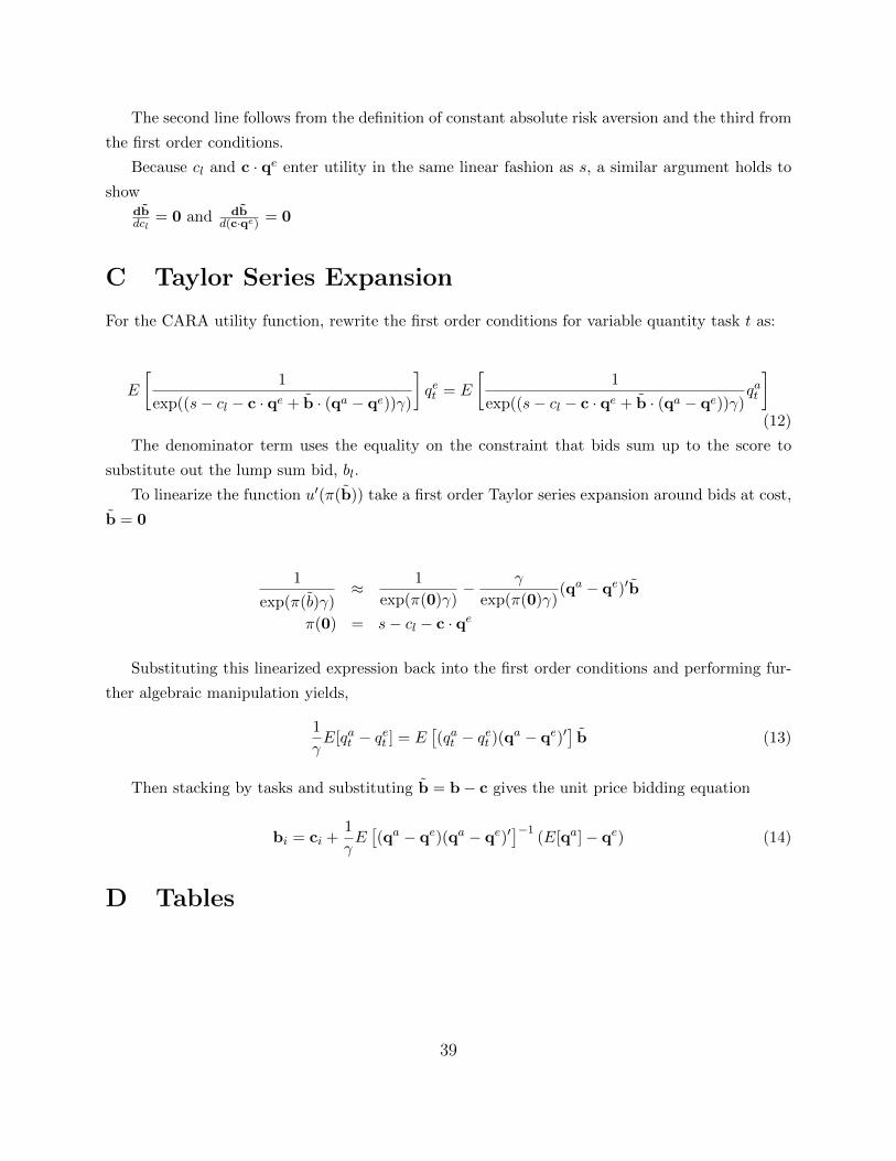
The second line follows from the definition of constant absolute risk aversion and the third from

the first order conditions.

Because cl and c · qe enter utility in the same linear fashion as s, a similar argument holds to

showdbdcl

= 0 and dbd(c·qe) = 0

C Taylor Series Expansion

For the CARA utility function, rewrite the first order conditions for variable quantity task t as:

E

[1

exp((s− cl − c · qe + b · (qa − qe))γ)

]qet = E

[1

exp((s− cl − c · qe + b · (qa − qe))γ)qat

](12)

The denominator term uses the equality on the constraint that bids sum up to the score to

substitute out the lump sum bid, bl.

To linearize the function u′(π(b)) take a first order Taylor series expansion around bids at cost,

b = 0

1

exp(π(b)γ)≈ 1

exp(π(0)γ)− γ

exp(π(0)γ)(qa − qe)′b

π(0) = s− cl − c · qe

Substituting this linearized expression back into the first order conditions and performing fur-

ther algebraic manipulation yields,

1

γE[qat − qet ] = E

[(qat − qet )(qa − qe)′

]b (13)

Then stacking by tasks and substituting b = b− c gives the unit price bidding equation

bi = ci +1

γE[(qa − qe)(qa − qe)′

]−1(E[qa]− qe) (14)

D Tables

39

Table 2: Construction Industry ListPercentof WorkSubcontracted

IndustryValueof WorkPerformed($)

Heavy Industries12.0% Concrete Structures 38,000,00012.0% Bituminous Seals 5,718,94815.8% Miscellaneous Metal 878,59916.0% Pipes Sewers Drainage 2,205,06717.0% Steel Structures 4,198,70922.8% Slope Protection 1,741,64223.0% Earthwork 16,200,00042.7% Shotcrete 130,04046.3% Asphalt Concrete 13,200,00047.8% Portland Cement Pavement 2,899,47085.5% Piling 10,700,00087.0% Prestressing Concrete 1,933,82299.3% Reinforcement 14,900,000

Total Heavy Industry Work 112,706,297Ancillary Industries

13.5% Markers And Delineators 31,29618.1% Traffic Control Devices 8,763,69443.5% Concrete Curbs And Sidewalks 1,248,13447.7% Clearing And Grubbing 620,46050.3% Waterproofing 205,62359.3% Existing Highway Facilities 7,460,88367.5% Railings And Barriers 4,957,76867.6% Signs 1,384,09771.6% Erosion Control And Planting 3,118,16583.4% Traffic Stripes And Markings 642,31586.7% Fences 303,89598.2% Electrical 3,445,87198.9% Painting 3,975,775

Total Ancillary Work 36,157,976Total All Work 148,864,273

Industry size based on winning bids. Subcontracting percentagebased on submitted bids. Nonstandard tasks excluded. Non-administrative lump sum tasks included. Noteworthy lump sumtask: “Remove Existing Bridge” in industry “Existing HighwayFacilities”. Remaining tasks are the removal of signs, barriersand traffic striping.

40

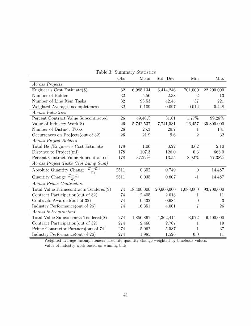
Table 3: Summary Statistics

Obs Mean Std. Dev. Min Max

Across Projects

Engineer’s Cost Estimate($) 32 6,985,134 6,414,246 701,000 22,200,000Number of Bidders 32 5.56 2.38 2 13Number of Line Item Tasks 32 93.53 42.45 37 221Weighted Average Incompleteness 32 0.109 0.097 0.012 0.448

Across Industries

Percent Contract Value Subcontracted 26 49.46% 31.61 1.77% 99.28%Value of Industry Work($) 26 5,742,537 7,741,581 26,457 35,800,000Number of Distinct Tasks 26 25.3 29.7 1 131Occurrences on Projects(out of 32) 26 21.9 9.6 2 32

Across Project Bidders

Total Bid/Engineer’s Cost Estimate 178 1.06 0.22 0.62 2.10Distance to Project(mi) 178 107.3 126.0 0.3 663.0Percent Contract Value Subcontracted 178 37.22% 13.55 8.92% 77.38%

Across Project Tasks (Not Lump Sum)

Absolute Quantity Change|qact−qect|qect

2511 0.302 0.749 0 14.487

Quantity Changeqact−qectqect

2511 0.035 0.807 -1 14.487

Across Prime Contractors

Total Value Primecontracts Tendered($) 74 18,400,000 20,600,000 1,083,000 93,700,000Contract Participation(out of 32) 74 2.405 2.013 1 11Contracts Awarded(out of 32) 74 0.432 0.684 0 3Industry Performance(out of 26) 74 16.351 4.001 7 26

Across Subcontractors

Total Value Subcontracts Tendered($) 274 1,856,867 4,362,414 3,072 46,400,000Contract Participation(out of 32) 274 2.460 2.767 1 19Prime Contractor Partners(out of 74) 274 5.062 5.587 1 37Industry Performance(out of 26) 274 1.985 1.526 0.0 11

Weighted average incompleteness: absolute quantity change weighted by bluebook values.Value of industry work based on winning bids.

41

Table 4: Summary Statistics: Variables Used in Estimation

Obs Mean Std. Dev. Min Max

Heavy Subcontracted

Incompleteness∣∣∣ qact−qectqect

∣∣∣ 1577 0.169 0.460 0 7.681∣∣∣ qact−qectqect

∣∣∣1(qact ≥ qect) 1577 0.075 0.413 0 7.681∣∣∣ qact−qectqect

∣∣∣1(qact < qect) 1577 0.094 0.236 0 1

Fringe (indicator) 1577 0.564 0.496 0 1Log Distance to Project 1577 4.099 1.276 -1.346 6.497

Task Scale Economiesqectqet

1577 1.095 1.035 0.0002 10.113

Normalized Unit Price Bid bcitcbbt

1577 1.901 2.362 0.001 32.648

Heavy Primecontracted

Incompleteness∣∣∣ qact−qectqect

∣∣∣ 3663 0.251 0.838 0 12.444∣∣∣ qact−qectqect

∣∣∣1(qact ≥ qect) 3663 0.146 0.819 0 12.444∣∣∣ qact−qectqect

∣∣∣1(qact < qect) 3663 0.105 0.251 0 1

Fringe (indicator) 3663 0.542 0.498 0 1Log Distance to Project 3663 3.937 1.223 -1.346 6.497

Task Scale Economiesqectqet

3663 1.083 1.225 0.0009 10.113

Normalized Unit Price Bid bcitcbbt

3663 2.016 2.682 0.001 50.036

Ancillary Subcontracted

Incompleteness∣∣∣ qact−qectqect

∣∣∣ 3597 0.379 0.754 0 10.735∣∣∣ qact−qectqect

∣∣∣1(qact ≥ qect) 3597 0.219 0.739 0 10.735∣∣∣ qact−qectqect

∣∣∣1(qact < qect) 3597 0.159 0.303 0 1

Fringe (indicator) 3597 0.535 0.499 0 1Log Distance to Project 3597 3.854 1.192 -1.346 6.497

Task Scale Economiesqectqet

3597 1.037 1.069 0.0002 10.986

Normalized Unit Price Bid bcitcbbt

3597 1.689 2.286 0.007 53.227

Ancillary Primecontracted

Incompleteness∣∣∣ qact−qectqect

∣∣∣ 3517 0.317 0.539 0 6.667∣∣∣ qact−qectqect

∣∣∣1(qact ≥ qect) 3517 0.159 0.497 0 6.667∣∣∣ qact−qectqect

∣∣∣1(qact < qect) 3517 0.158 0.305 0 1

Fringe (indicator) 3517 0.560 0.497 0 1Log Distance to Project 3517 3.997 1.213 -1.346 6.497

Task Scale Economiesqectqet

3517 0.973 0.929 0.0002 7.423

Normalized Unit Price Bid bcitcbbt

3517 1.980 4.678 0.001 189.251

42

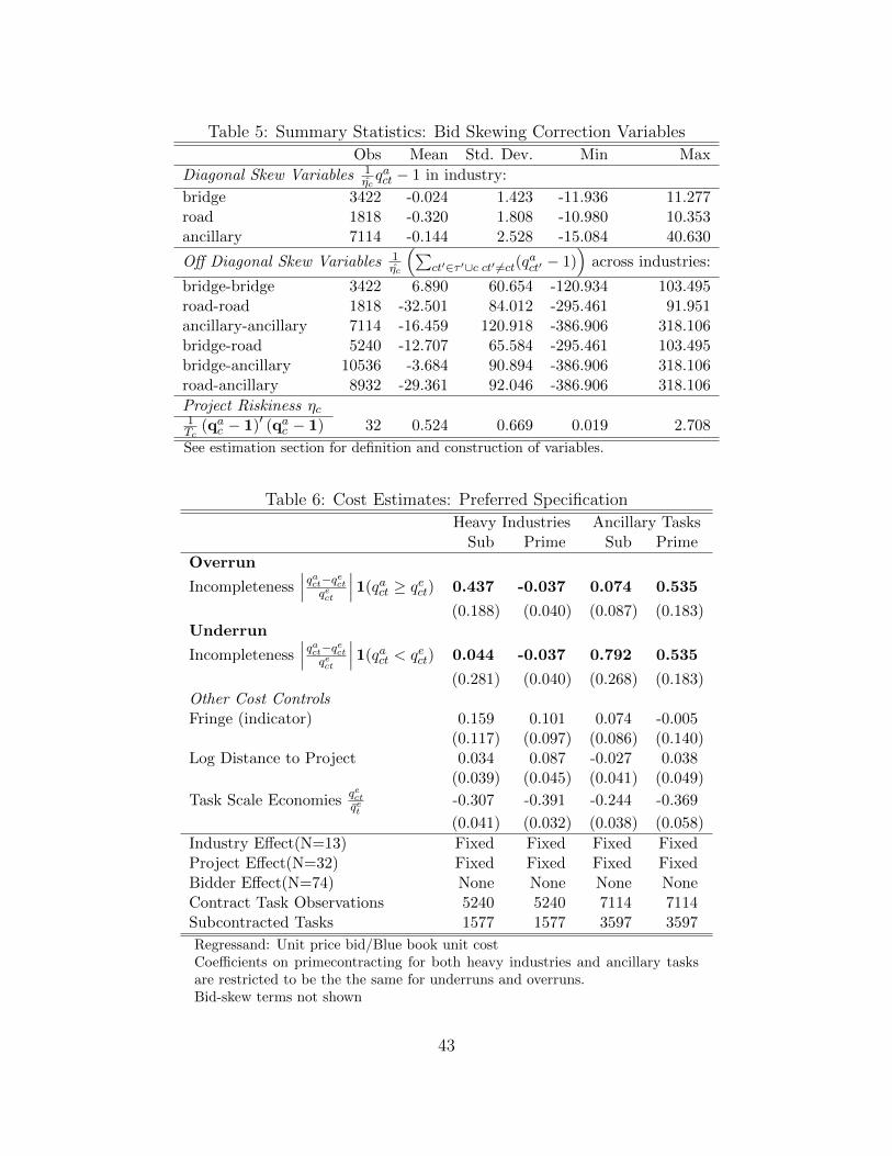
Table 5: Summary Statistics: Bid Skewing Correction Variables

Obs Mean Std. Dev. Min Max

Diagonal Skew Variables 1ηcqact − 1 in industry:

bridge 3422 -0.024 1.423 -11.936 11.277road 1818 -0.320 1.808 -10.980 10.353ancillary 7114 -0.144 2.528 -15.084 40.630

Off Diagonal Skew Variables 1ηc

(∑ct′∈τ ′∪c ct′ 6=ct(q

act′ − 1)

)across industries:

bridge-bridge 3422 6.890 60.654 -120.934 103.495road-road 1818 -32.501 84.012 -295.461 91.951ancillary-ancillary 7114 -16.459 120.918 -386.906 318.106bridge-road 5240 -12.707 65.584 -295.461 103.495bridge-ancillary 10536 -3.684 90.894 -386.906 318.106road-ancillary 8932 -29.361 92.046 -386.906 318.106

Project Riskiness ηc1Tc

(qac − 1)′ (qac − 1) 32 0.524 0.669 0.019 2.708

See estimation section for definition and construction of variables.

Table 6: Cost Estimates: Preferred Specification

Heavy Industries Ancillary TasksSub Prime Sub Prime

Overrun

Incompleteness∣∣∣ qact−qectqect

∣∣∣1(qact ≥ qect) 0.437 -0.037 0.074 0.535

(0.188) (0.040) (0.087) (0.183)Underrun

Incompleteness∣∣∣ qact−qectqect

∣∣∣1(qact < qect) 0.044 -0.037 0.792 0.535

(0.281) (0.040) (0.268) (0.183)Other Cost ControlsFringe (indicator) 0.159 0.101 0.074 -0.005

(0.117) (0.097) (0.086) (0.140)Log Distance to Project 0.034 0.087 -0.027 0.038

(0.039) (0.045) (0.041) (0.049)

Task Scale Economiesqectqet

-0.307 -0.391 -0.244 -0.369

(0.041) (0.032) (0.038) (0.058)

Industry Effect(N=13) Fixed Fixed Fixed FixedProject Effect(N=32) Fixed Fixed Fixed FixedBidder Effect(N=74) None None None NoneContract Task Observations 5240 5240 7114 7114Subcontracted Tasks 1577 1577 3597 3597

Regressand: Unit price bid/Blue book unit costCoefficients on primecontracting for both heavy industries and ancillary tasksare restricted to be the the same for underruns and overruns.Bid-skew terms not shown

43

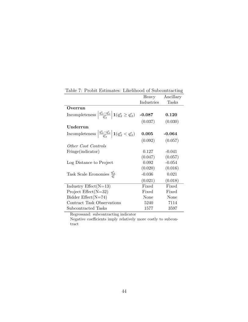
Table 7: Probit Estimates: Likelihood of Subcontracting

Heavy AncillaryIndustries Tasks

Overrun

Incompleteness∣∣∣ qact−qectqect

∣∣∣1(qact ≥ qect) -0.087 0.120

(0.037) (0.030)Underrun

Incompleteness∣∣∣ qact−qectqect

∣∣∣1(qact < qect) 0.005 -0.064

(0.092) (0.057)Other Cost ControlsFringe(indicator) 0.127 -0.041

(0.047) (0.057)Log Distance to Project 0.092 -0.054

(0.020) (0.016)

Task Scale Economiesqectqet

-0.036 0.021

(0.021) (0.018)

Industry Effect(N=13) Fixed FixedProject Effect(N=32) Fixed FixedBidder Effect(N=74) None NoneContract Task Observations 5240 7114Subcontracted Tasks 1577 3597

Regressand: subcontracting indicatorNegative coefficients imply relatively more costly to subcon-tract

44

Table 8: Skew Matrix Estimates: Restricted & Preferred Specification

(A = V−1) Inverse Covariance MatrixBridge Road Ancillary

Bridge (diagonal) 0.0804(0.0263)

Bridge (off diagonal) 0.0196(0.0043)

Road (diagonal) 0.0754(0.0445)

Road (off diagonal) 0.0100 0.0067(0.0037) (0.0037)

Ancillary (diagonal) 0.0398(0.0289)

Ancillary (off diagonal) -0.0026 0.0004 0.0005(0.0041) (0.0041) (0.0015)

(V) Covariance Matrix

Bridge (diagonal) 13.52Bridge (off diagonal) -2.93Road (diagonal) 13.69Road (off diagonal) -1.30 -0.87Ancillary (diagonal) 25.23Ancillary (off diagonal) 0.71 -0.29 -0.22

standard errors in parentheses.Matrix (A) estimated from bid data. Matrix (V) inverse ofmatrix (A) point estimates.See estimation section for description of matrices and estima-tion procedure.Preferred specification with coefficient restrictions on contrac-tual incompleteness for primecontracting.

45

Table 9: Skew Matrix Estimates: Unrestricted & Biased Specification

(A = V−1) Inverse Covariance MatrixBridge Road Ancillary

Bridge (diagonal) 0.0655(0.0304)

Bridge (off diagonal) 0.0196(0.0043)

Road (diagonal) 0.0600(0.0427)

Road (off diagonal) 0.0100 0.0068(0.0037) (0.0037)

Ancillary (diagonal) 0.0248(0.0323)

Ancillary (off diagonal) -0.0026 0.0004 0.0005(0.0041) (0.0041) (0.0015)

(V) Covariance Matrix

Bridge (diagonal) 17.31Bridge (off diagonal) -4.48Road (diagonal) 17.47Road (off diagonal) -1.94 -1.33Ancillary (diagonal) 40.64Ancillary (off diagonal) 1.38 -0.65 -0.51

standard errors in parentheses.Matrix (A) estimated from bid data. Matrix (V) inverse ofmatrix (A) point estimates.See estimation section for description of matrices and estima-tion procedure.Biased specification with no restrictions on contractual incom-pleteness for primecontracting.

46

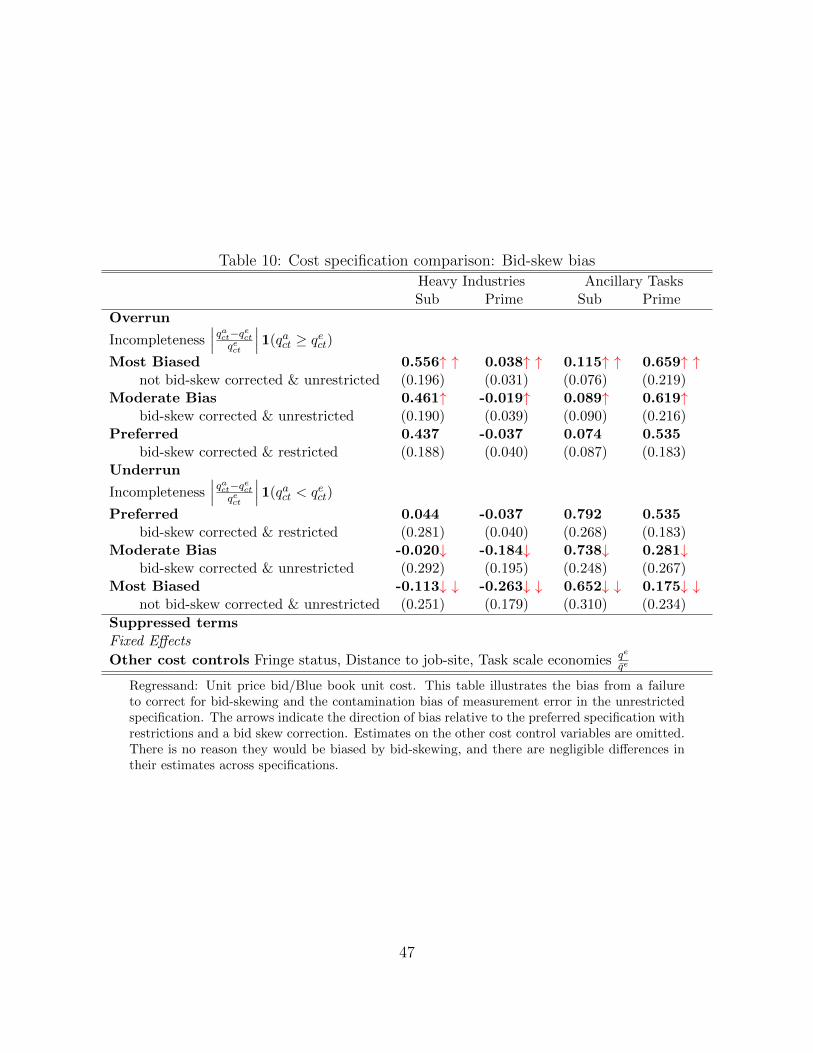
Table 10: Cost specification comparison: Bid-skew bias

Heavy Industries Ancillary TasksSub Prime Sub Prime

Overrun

Incompleteness∣∣∣ qact−qectqect

∣∣∣1(qact ≥ qect)Most Biased 0.556↑ ↑ 0.038↑ ↑ 0.115↑ ↑ 0.659↑ ↑

not bid-skew corrected & unrestricted (0.196) (0.031) (0.076) (0.219)Moderate Bias 0.461↑ -0.019↑ 0.089↑ 0.619↑

bid-skew corrected & unrestricted (0.190) (0.039) (0.090) (0.216)Preferred 0.437 -0.037 0.074 0.535

bid-skew corrected & restricted (0.188) (0.040) (0.087) (0.183)Underrun

Incompleteness∣∣∣ qact−qectqect

∣∣∣1(qact < qect)

Preferred 0.044 -0.037 0.792 0.535bid-skew corrected & restricted (0.281) (0.040) (0.268) (0.183)

Moderate Bias -0.020↓ -0.184↓ 0.738↓ 0.281↓bid-skew corrected & unrestricted (0.292) (0.195) (0.248) (0.267)

Most Biased -0.113↓ ↓ -0.263↓ ↓ 0.652↓ ↓ 0.175↓ ↓not bid-skew corrected & unrestricted (0.251) (0.179) (0.310) (0.234)

Suppressed termsFixed Effects

Other cost controls Fringe status, Distance to job-site, Task scale economies qe

qe

Regressand: Unit price bid/Blue book unit cost. This table illustrates the bias from a failureto correct for bid-skewing and the contamination bias of measurement error in the unrestrictedspecification. The arrows indicate the direction of bias relative to the preferred specification withrestrictions and a bid skew correction. Estimates on the other cost control variables are omitted.There is no reason they would be biased by bid-skewing, and there are negligible differences intheir estimates across specifications.

47