Sub-Riemannian vs. Euclidean dimension …Sub-Riemannian vs. Euclidean dimension comparison and...

$: Sub-Riemannian vs. Euclidean dimension …Sub-Riemannian vs. Euclidean dimension comparison and fractal geometry on Carnot groups Zoltán M. Balogha,1, Jeremy T. Tysonb,∗,2, Ben$
Advances in Mathematics 220 (2009) 560–619www.elsevier.com/locate/aim

Sub-Riemannian vs. Euclidean dimension comparisonand fractal geometry on Carnot groups

Zoltán M. Balogh a,1, Jeremy T. Tyson b,∗,2, Ben Warhurst c,3

a Department of Mathematics, University of Bern, Sidlerstrasse 5, 3012 Bern, Switzerlandb Department of Mathematics, University of Illinois, 1409 W. Green St., Urbana, IL 61801, USA

c School of Mathematics, University of New South Wales, Sydney 2052, Australia

Received 14 March 2008; accepted 16 September 2008

Available online 29 October 2008

Communicated by Kenneth Falconer

Dedicated to the memory of Juha Heinonen (1960–2007)4

Abstract

We solve Gromov’s dimension comparison problem for Hausdorff and box counting dimension on Carnotgroups equipped with a Carnot–Carathéodory metric and an adapted Euclidean metric. The proofs use sharpcovering theorems relating optimal mutual coverings of Euclidean and Carnot–Carathéodory balls, andelements of sub-Riemannian fractal geometry associated to horizontal self-similar iterated function systemson Carnot groups. Inspired by Falconer’s work on almost sure dimensions of Euclidean self-affine fractalswe show that Carnot–Carathéodory self-similar fractals are almost surely horizontal. As a consequence weobtain explicit dimension formulae for invariant sets of Euclidean iterated function systems of polynomialtype. Jet space Carnot groups provide a rich source of examples.© 2008 Elsevier Inc. All rights reserved.

* Corresponding author.E-mail addresses: [email protected] (Z.M. Balogh), [email protected] (J.T. Tyson),

[email protected] (B. Warhurst).1 Supported by the Swiss Nationalfond, EC Project GALA “Sub-Riemannian geometric analysis in Lie groups” and

ERC Project HCAA “Harmonic and Complex Analysis and its Applications.”2 Supported by NSF grant DMS 0555869 “Nonsmooth methods in geometric function theory and geometric measure

theory on the Heisenberg group.”3 Supported by ARC Discovery grant “Geometry of Nilpotent Groups.”4 We dedicate this paper to the memory of Juha Heinonen, mentor and friend who inspired us in mathematics and in

other areas of life.

0001-8708/$ – see front matter © 2008 Elsevier Inc. All rights reserved.doi:10.1016/j.aim.2008.09.018

Z.M. Balogh et al. / Advances in Mathematics 220 (2009) 560–619 561

Keywords: Carnot group; Hausdorff dimension; Iterated function system; Self-similar fractal

Contents

1. Introduction . . . . . . . . . . . . . . . . . . . . . . . . . . . . . . . . . . . . . . . . . . . . . . . . . . . . . 5612. Notation and statements of main results . . . . . . . . . . . . . . . . . . . . . . . . . . . . . . . . . . . 565

2.1. Carnot groups . . . . . . . . . . . . . . . . . . . . . . . . . . . . . . . . . . . . . . . . . . . . . . . 5652.2. Carnot–Carathéodory metric . . . . . . . . . . . . . . . . . . . . . . . . . . . . . . . . . . . . . 5672.3. Hausdorff and box-counting dimensions . . . . . . . . . . . . . . . . . . . . . . . . . . . . . 5682.4. Statements of the main results and discussion . . . . . . . . . . . . . . . . . . . . . . . . . . 569

3. Proof of the dimension comparison theorem . . . . . . . . . . . . . . . . . . . . . . . . . . . . . . . . 5754. Sharpness of the dimension comparison theorem . . . . . . . . . . . . . . . . . . . . . . . . . . . . . 583

4.1. Vertical sets . . . . . . . . . . . . . . . . . . . . . . . . . . . . . . . . . . . . . . . . . . . . . . . . . 5834.2. Horizontal sets . . . . . . . . . . . . . . . . . . . . . . . . . . . . . . . . . . . . . . . . . . . . . . . 587

5. CC self-similar invariant sets in Carnot groups are almost surely horizontal . . . . . . . . . . . 5965.1. Symbolic dynamics and iterated function systems . . . . . . . . . . . . . . . . . . . . . . . 5985.2. Proof of Theorem 2.8 . . . . . . . . . . . . . . . . . . . . . . . . . . . . . . . . . . . . . . . . . . 599

6. Jet spaces . . . . . . . . . . . . . . . . . . . . . . . . . . . . . . . . . . . . . . . . . . . . . . . . . . . . . . . 6046.1. Jet spaces as Carnot groups: the classical model . . . . . . . . . . . . . . . . . . . . . . . . 6046.2. Jet spaces as Carnot groups: an alternate model . . . . . . . . . . . . . . . . . . . . . . . . . 6066.3. A relation between self-similar sub-Riemannian fractal geometry and self-affine Euclidean

fractal geometry in jet spaces . . . . . . . . . . . . . . . . . . . . . . . . . . . . . . . . . . . . . 6077. Another example . . . . . . . . . . . . . . . . . . . . . . . . . . . . . . . . . . . . . . . . . . . . . . . . . . 6108. Open problems and questions . . . . . . . . . . . . . . . . . . . . . . . . . . . . . . . . . . . . . . . . . . 611

8.1. Remarks concerning Problems 1.1 and 1.2 . . . . . . . . . . . . . . . . . . . . . . . . . . . . 6128.2. Dimension comparison for submanifolds . . . . . . . . . . . . . . . . . . . . . . . . . . . . . 6138.3. Hausdorff measure sharpness in the dimension comparison theorem . . . . . . . . . . . 6148.4. Topological structure of Carnot fractals . . . . . . . . . . . . . . . . . . . . . . . . . . . . . . 6148.5. Exceptional sets . . . . . . . . . . . . . . . . . . . . . . . . . . . . . . . . . . . . . . . . . . . . . . 6148.6. Carnot–Carathéodory manifolds . . . . . . . . . . . . . . . . . . . . . . . . . . . . . . . . . . . 6158.7. Other metric spaces . . . . . . . . . . . . . . . . . . . . . . . . . . . . . . . . . . . . . . . . . . . 616

Acknowledgments . . . . . . . . . . . . . . . . . . . . . . . . . . . . . . . . . . . . . . . . . . . . . . . . . . . . . . 617References . . . . . . . . . . . . . . . . . . . . . . . . . . . . . . . . . . . . . . . . . . . . . . . . . . . . . . . . . . . 617

1. Introduction

Carnot groups are simply connected nilpotent Lie groups with graded Lie algebra equippedwith a left invariant metric of sub-Riemannian type. They arise as ideal boundaries of noncom-pact rank one symmetric spaces, and serve as both examples of, and local models at regularpoints for, general sub-Riemannian (Carnot–Carathéodory) manifolds. The key role played byCarnot groups became evident in the 1970s in a series of influential papers and monographs(such as [55,53,25]) following the address by E.M. Stein at the 1970 International Congress ofMathematicians in Nice. More recently, Carnot groups have played a significant role in motivat-ing the development of analysis in metric measure spaces, see particularly the work of Heinonenand Koskela [33,34], Cheeger [15] and Ambrosio and Kirchheim [1,2]. In this respect Carnotgroups serve as models for non-Euclidean examples of spaces where the above cited results can

562 Z.M. Balogh et al. / Advances in Mathematics 220 (2009) 560–619

be tested. On the other hand, it is well known that tools of Carnot–Carathéodory analysis are alsomotivated by applications in control theory [50,9,38]. Recently, the rototranslation group (a sub-Riemannian manifold locally modelled on the Heisenberg group) has emerged as a mathematicalmodel for the neurogeometry of the first layer of the mammalian visual cortex [16].

This paper develops a theory of self-similar fractal geometry in general Carnot groups. Itcontinues our program in this area [5,4,7], which is one component in a worldwide endeavorinvestigating sub-Riemannian geometric measure theory, including theories of rectifiability andperimeter [14,26,27,17,44,3,40]; fractals and tilings [58,59]; and geometric analysis of nons-mooth domains [28,42,52,51].

Gromov [30,31] has advocated a program to study the intrinsic metric geometry of Carnot–Carathéodory (CC) spaces. The present work originated in our consideration of the followingproblem, posed in [31, §3.1] (see also [30, Problem 0.6.C]):

Problem 1.1 (Gromov). Let M be a manifold equipped with a horizontal distribution H ⊂ T M

and sub-Riemannian (Carnot–Carathéodory) metric g0 with associated distance function d0. Foreach k = 0,1, . . . ,dimM , determine

βk := inf{dimH

d0S: S ⊂ M, S compact, dimtop S = k

}. (1.1)

Here dimHd denotes Hausdorff dimension in a metric space (X,d) and dimtop stands for the

topological dimension.More generally, one may ask for a characterization of the set{

(k,β): ∃S ⊂ M, S Borel, dimtop S = k, dimHd0

S = β}. (1.2)

In the case when M is a Carnot group, our main results (described below) imply that for each k,the set of values of dimH

d0S, where S varies over Borel subsets of M of topological dimen-

sion k, is an interval. We conjecture that {β: ∃S ⊂ M, S Borel, dimtop S = k, dimHd0

S = β} =[βk,dimH

d0M] for each k. See Remark 8.1 for additional remarks, conjectures and discussion.

The computation of βk is in general extremely challenging. It is clear that βk = k for suffi-ciently small k, in fact, for any k such that M contains an isometrically embedded Riemanniank-manifold. Thus βk = k for k = 1, . . . , n when M = Hn is the nth Heisenberg group. On theother hand,

βdimM−1 = dimHd0

M − 1 > dimM − 1 (1.3)

for regular sub-Riemannian but non-Riemannian manifolds M , and especially in nonabelianCarnot groups; see [30, §2.1]. In particular, β1 = 1 and β2 = 3 in the first Heisenberg group H1.

It is of interest to pose Problem 1.1 for restricted classes of subsets of M , for instance, forsmooth submanifolds. Gromov [30, §0.6] gives an explicit formula for the CC Hausdorff dimen-sion of a general submanifold of a (regular) sub-Riemannian manifold. We illustrate with the firstHeisenberg group H1. Denoting by β the CC Hausdorff dimension of a smooth k-dimensionalsubmanifold in H1, we observe that only the following pairs (k,β) can occur:{

(0,0), (1,1), (1,2), (2,3), (3,4)}. (1.4)


Examples which realize each case in (1.4) are (respectively): singletons, horizontal curves, non-horizontal curves, smooth surfaces, and the entire space H1. The absence of the pair (2,2) in thislist indicates that there is no smooth surface in the first Heisenberg group which has dimensiontwo with respect to the sub-Riemannian metric. This feature of the geometry reflects the non-integrability of the horizontal distribution as indicated by the failure of the Frobenius theorem.We discuss Gromov’s dimension comparison problem for smooth submanifolds in more detail inRemark 8.2.

A more ambitious goal is the following problem.

Problem 1.2. Let M be as in Problem 1.1 and let g be a Riemannian metric which extends g0.Determine explicitly the set of triples (k,α,β) arising as the topological, Riemannian Hausdorffand sub-Riemannian Hausdorff dimensions of Borel subsets of M . More precisely, compute

Δ(M) = {(k,α,β): ∃S ⊂ M, S Borel, dimtop S = k, dimHd S = α, dimH

d0S = β

},

where d denotes the distance function determined by g.

The set in (1.2) is the projection of Δ(M) in the (k,β)-plane. Alternatively, we may considerthe projection of Δ(M) in the (α,β)-plane. Since the Hausdorff measures are Borel regular, wecan drop the restriction to Borel sets at this stage. Thus we are led to the following problem:

Problem 1.3. Let M be as in Problem 1.1. Determine explicitly the set of pairs (α,β) arising asthe Riemannian/sub-Riemannian Hausdorff dimensions of subsets of M . More precisely, com-pute

Δ′(M) := {(α,β) ∈ R2: ∃S ⊂ M, dimHd S = α, dimH

d0S = β

}. (1.5)

Problem 1.3 is a foundational question in sub-Riemannian geometric measure theory whichasks for a quantitative description of the discrepancy between the sub-Riemannian metric g0 andany taming Riemannian metric g. In this paper, we give a complete solution to Problem 1.3 inthe case when M is a Carnot group. We shall see that this problem asks which Riemannian α-dimensional subsets of M are most nearly horizontal (β is smallest for fixed α) and which aremost non-horizontal (β is largest for fixed α). The intuitive meaning of the phrase “horizontalset” is a set which is tangent to the horizontal distribution in M . We emphasize, however, thatour framework is that of general geometric measure theory, and the examples which we willconstruct are typically not smooth submanifolds from either the Euclidean or the sub-Riemannianviewpoint.

Let G be a Carnot group equipped with a sub-Riemannian metric, of topological dimension N

and homogeneous dimension Q. (See Section 2 for a review of definitions and terminology.) Wewill determine explicit functions β± = βG± : [0,N] → [0,Q] so that

Δ′(G) = {(α,β) ∈ [0,N] × [0,Q]: β−(α) � β � β+(α)}. (1.6)

See Theorems 2.4 and 2.6.The results of this paper extend our prior work [5,7] on the Heisenberg group H1. We recall

from [5] and [7] that the solution to Problem 1.3 when M = H1 is


Fig. 1. Solution to Problem 1.3 in H1.

Δ′(H1)= {(α,β) ∈ [0,3] × [0,4]: βH1

− (α) = max{α,2α − 2} � β � βH1

+ (α)

= min{2α,α + 1}}. (1.7)

See Fig. 1 for an illustration of (1.4) and (1.7). In Fig. 1 the set Δ′(H1) is represented by theshaded parallelogram while the points in (1.4) are represented by circled dots at the integercoordinates on the edges and corners. Notice the absence of (2,2).

The solution to Problem 1.3 on a Carnot group G involves two stages. In the first stage we de-termine a region Δ′(G) in R2 where all possible dimension pairs are located. This stage utilizesprecise mutual coverings of Euclidean, respectively Carnot–Carathéodory, balls which general-ize the well-known Ball–Box Theorem [30,9]. In the second stage we prove a sharpness result:for any (α,β) ∈ Δ′(G), there exists a compact set S = Sα,β ⊂ G of topological dimension zerowith dimH

d S = α and dimHd0

S = β . To tackle the issue of sharpness we have to actually con-struct sets of prescribed Euclidean dimension whose Carnot–Carathéodory dimension is eitheras small or as large as possible as allowed by the first part of our result. Constructing sets ofmaximal Carnot–Carathéodory dimension is relatively straightforward while constructing setswith minimal Carnot–Carathéodory dimension is considerably harder. The difficulty is due tothe non-integrability of the horizontal distribution.

The construction of examples demonstrating sharpness in our solution to Problem 1.3 relieson a theory of fractal geometry in Carnot groups. The development of such a theory is the secondmain goal of this paper. We shall consider self-similar iterated function systems and their invari-ant sets. The notion of self-similarity is understood here in terms of the Carnot–Carathéodory(CC) metric. The associated iterated function system will (typically) be a nonlinear, nonconfor-mal system of polynomial type in the underlying Euclidean space. Let us mention that in ourprevious work [5] and [7] we also considered fractal sets in the setting of the Heisenberg groupin connection with Gromov’s problem. The iterated function systems we considered were affineEuclidean. Working in higher step Carnot groups, we have to deal with additional difficultiesdue to the non-linearity of the group law. One remarkable feature of our approach is that, as abyproduct of our investigations of sub-Riemannian self-similar fractals, we obtain exact formu-las for the dimensions of invariant sets for a class of nonlinear, nonconformal Euclidean iteratedfunction systems of polynomial type. These results are related to [20] and [22]. Example 2.10(see also the discussion at the end of Subsection 4.2) and Section 7 indicate representative ex-amples. Our approach provides a dramatic simplification over existing methods for computing


such dimensions (see Falconer [23] for an approach using a nonconformal subadditive thermo-dynamic formalism). Our investigation of Carnot fractal geometry culminates in Theorem 2.8,which states, roughly speaking, that CC self-similar sets of prescribed sub-Riemannian dimen-sion are almost surely horizontal sets (in the sense described above).

Our main results (Theorems 2.4, 2.6 and 2.8) hold also for box-counting dimension, see thediscussion at the end of Section 3 and Remarks 4.5 and 4.17. Box-counting and Hausdorff di-mension each play an important role in the study of attractors for general nonlinear iteratedfunction systems, see [23]. It is a long-standing conjecture in dynamical systems that equalityof these dimensions holds for such attractors in great generality, see [24] or [35]. The fact thatour results hold for both Hausdorff and box-counting dimension, and that typically we obtainequality of these two values, is an essential feature of our approach with immediate applicationsto Euclidean fractal geometry.

The jet spaces J k(Rm,Rn) provide a rich source of examples of Carnot groups. In Section 6we illustrate our results by discussing in detail the form which they take in the jet space context.We present a second Carnot group model for J k(R,R) in which left translation is an affinemap in the underlying Euclidean geometry, whose linear part is given by a triangular matrix.In Subsection 6.3 we relate our work to recent work of Falconer and Miao [18] on almost suredimensions of invariant sets of self-affine iterated function systems whose linear parts are givenby upper triangular matrices. In Remark 6.5 we give the complete solution to Problem 1.2 in thesecond jet group J 2(R,R).

The paper is structured as follows. In Section 2 we recall basic definitions, set notation andformulate our main results as Theorems 2.4, 2.6 and 2.8. Sections 3 and 4 contain the proofsof Theorems 2.4 and 2.6 respectively. In Section 5 we extend Falconer’s almost sure dimensiontheory to the setting of Carnot self-similar fractals and prove Theorem 2.8. Section 6 discussesjet spaces, while Section 7 describes a more complicated example of a higher-step Carnot group.A concluding section (Section 8) presents additional remarks and open problems motivated bythis work.

Some of the results of this paper were announced in [8].

2. Notation and statements of main results

2.1. Carnot groups

Let (G,∗) be a Carnot group with stratified Lie algebra g = v1 ⊕ · · · ⊕ vs such that[v1,vj ] = vj+1, j = 1, . . . , s − 1, and [v1,vs] = 0. The Euclidean space underlying G hasdimension N =∑s

j=1 mj while the homogeneous dimension of G is Q =∑sj=1 jmj , where

dimvj = mj , and s is the step of the group. We denote by dE the Euclidean metric in G.The map on g which multiplies the elements of the j th stratum vj by j is a derivation. It

generates a group of automorphic anisotropic dilations {δr : r ∈ R+} of g defined by

δr (U1 + · · · + Us) = rU1 + · · · + rsUs, Uj ∈ vj ,

with the property that δrδt = δrt . We will also write δr for the corresponding automorphismexp◦δr ◦ log : G → G; here exp denotes the (bijective) exponential map and log denotes its in-verse.


The exponential map exp :g → G relates also to the group operation in G via the Baker–Campbell–Hausdorff formula [54] as follows. For U and V in g

exp(U) ∗ exp(V ) = exp(BCH(U,V )

), (2.1)

where

BCH(U,V ) = U + V + 1

2[U,V ] + 1

12

([U, [U,V ]]− [V, [U,V ]])+ · · · .

Since exp is a bijection we may parametrize G by g. Exponential coordinates in G are defined asfollows: denoting by {Ejk: j = 1, . . . , s; k = 1, . . . ,mj } a graded orthonormal basis for g (withrespect to some fixed inner product) and by {ejk: k = 1, . . . ,mj } the standard orthonormal basisof Rmj , we identify x ∈ G with the point (x1, . . . , xs) ∈ Rm1 × · · · × Rms where

x = exp

(s∑

j=1

mj∑k=1

〈xj , ejk〉Ejk

).

We denote by πj : G → Rmj the projection, given in exponential coordinates asπj (x1, . . . , xs) = xj .

The Haar measure on G, obtained by pushing forward the Lebesgue measure on g, is transla-tion invariant. In exponential coordinates, this is just the Lebesgue measure on RN . If we denoteby |E| the measure of a set E, then |δr (E)| = rQ|E|.

We can identify the Lie algebra g with the tangent space ToG of G at the neutral elemento ∈ G. For U ∈ g we have a unique left invariant vector field X = XU on G which agreeswith U at o. Vector fields corresponding to vectors in vj span a vector bundle Vj over G ofdimension mj which varies smoothly from point to point. The hypothesis on the Lie algebrastratification implies that for all j = 1, . . . , s sections of Vj are obtained by taking linear combi-nations of commutators up to order j of vector fields in the first stratum V1 (called the horizontaldistribution). We denote by HG the horizontal distribution in G.

Example 2.1. We model the Heisenberg group Hn with the polynomial group law on R2n+1

given by

p ∗ q =(

x1 + y1, . . . , x2n + y2n, x2n+1 + y2n+1 + 1

2

n∑j=1

(xj yn+j − xn+j yj )

),

where p = (x1, . . . , x2n+1) and q = (y1, . . . , y2n+1). This is a step two Carnot group of dimen-sion N = 2n+1 with stratified Lie algebra g = v1 ⊕v2, where v1 and v2 correspond to the vectorbundles V1 = span{X1, . . . ,X2n} and V2 = span{X2n+1},

Xj = ∂

∂xj

− 1

2xn+j

∂

∂x2n+1and Xn+j = ∂

∂xn+j

+ 1

2xj

∂

∂x2n+1for j = 1, . . . , n,

and

X2n+1 = ∂.

∂x2n+1


The nontrivial commutation relations in g are [Xj ,Xn+j ] = X2n+1 for each j = 1, . . . , n. Thehomogeneous dimension of Hn is Q = 2n + 2.

Example 2.2. We model the Engel group E with the polynomial group law on R4 given by

x ∗ y =(

x1 + y1, x2 + y2, x3 + y3 + x2y1, x4 + y4 + x3y1 + 1

2x2y

21

),

where x = (x1, x2, x3, x4) and y = (y1, y2, y3, y4). This is a step three Carnot group of dimensionN = 4 with stratified Lie algebra g = v1 ⊕ v2 ⊕ v3, where v1, v2 and v3 correspond to the vectorbundles V1 = span{U1,U2}, V2 = span{V }, and V3 = span{W },

U1 = ∂

∂x1, U2 = ∂

∂x2+ x1

∂

∂x3+ 1

2x2

1∂

∂x4, V = ∂

∂x3+ x1

∂

∂x4, and W = ∂

∂x4.

The nontrivial commutation relations are [U1,U2] = V and [U1,V ] = W . The homogeneousdimension of E can easily be calculated as Q = 2+1 ·2+1 ·3 = 7. The Engel group is isomorphicwith the second jet group J 2(R,R); see Section 6 for a review of the Carnot structure of jetspaces.

2.2. Carnot–Carathéodory metric

We equip v1 with an inner product 〈·,·〉 (for instance, by restricting the above inner producton g) and extend it as a left invariant inner product on V1. The Carnot–Carathéodory (CC) met-ric dcc is the standard sub-Riemannian metric defined using this inner product. For x, y ∈ G,dcc(x, y) is the infimum of the lengths of all horizontal paths joining x and y. Here an absolutelycontinuous path γ : [0,1] → G is said to be horizontal if its tangents lie in the horizontal bun-dle V1 almost everywhere, i.e., γ ′(t) ∈ (V1)γ (t) for almost every t ∈ [0,1], and the length of γ is∫ 1

0 〈γ ′(t), γ ′(t)〉1/2γ (t)

dt . Note that because of the bracket generating property of V1, and in view ofChow’s theorem [9,30], every pair of points x, y ∈ G can be joined by a horizontal path, whencedcc(x, y) is finite.

The Carnot–Carathéodory metric is left invariant: dcc(x ∗ y, x ∗ z) = dcc(y, z) for allx, y, z ∈ G, and compatible with the dilations: dcc(δr (x), δr (y)) = rdcc(x, y) for all x, y ∈ G

and r > 0. We write |x|cc = dcc(x, o) and |x|E = dE(x, o). Observe that

|x|E � |x|cc for all x ∈ G, (2.2)

with equality if x = (x1,0, . . . ,0) in exponential coordinates (since in this case γ : [0,1] → G,γ (t) = δt (x), is horizontal). An immediate consequence of (2.2) and (2.1) is the following fact:

π1 : (G, dcc) → (Rm1, dE

)is 1-Lipschitz. (2.3)

Note that πj is never Lipschitz from (G, dcc) to (Rmj , dE) when j � 2, see [9] or [30].The topology generated by the Carnot–Carathéodory metric is the same as that defined by

the Euclidean metric on the underlying space. However the two metrics are never bi-Lipschitzequivalent if s > 1. If we denote by Bcc(p, r) the CC ball centered at p ∈ G of radius r > 0we see that |Bcc(p, r)| = rQ|Bcc(0,1)| which implies that the Hausdorff dimension of G with


respect to the CC metric is equal to Q. Evidently, Q > N when G is nonabelian, i.e., s > 1. Forexample,

Q = 2n + 2 = dimcc Hn > dimE Hn = 2n + 1 = N.

In the case of the Engel group E the difference is even more dramatic:

Q = 7 = dimcc E > dimE E = 4 = N.

One of the main goals of this paper is to compare the Hausdorff dimensions of arbitrary subsetsof arbitrary Carnot groups as measured with the Euclidean versus the CC metric.

2.3. Hausdorff and box-counting dimensions

In order to state our main results let us quickly recall for the sake of completeness the defini-tions of Hausdorff measure and Hausdorff and box-counting dimension in the general setting ofa metric space (X,d). (For more information see [21,39,47].) Given A ⊂ X, the diameter of A is

diam(X,d)(A) = sup{d(x, y): x, y ∈ A

}.

We write diam = diam(X,d) when there is no risk of confusion, and abbreviate diamE =diam(G,dE) and diamcc = diam(G,dcc).

For 0 � t < ∞, 0 < δ � ∞ and A ⊂ X, the t-dimensional Hausdorff premeasure of A is

Ht(X,d),δ(A) = inf

∞∑i=1

diam(Ai)t ,

where the infimum is taken over all coverings of A by sets {Ai} with diameter at most δ. Forfixed t and A, the quantity Ht

(X,d),δ(A) is non-decreasing in δ; the quantity

Ht(X,d)(A) = Ht

(X,d),0(A) := supδ>0

Ht(X,d),δ(A)

is the t-dimensional Hausdorff measure of A. The Hausdorff dimension of A is

dimH(X,d) A := inf

{t � 0: Ht

(X,d)(A) = 0}.

As before we abbreviate Ht(G,dE),δ

= HtE,δ and Ht

(G,dcc),δ= Ht

cc,δ and write dimHE , dimH

cc for thecorresponding Hausdorff dimensions.

Let us turn now to the definition of the box-counting dimension. For ε > 0 and a bounded setA ⊂ X we let N(X,d)(A, ε) be the minimum number of sets of diameter ε needed to cover A. Thelower (resp. upper) box-counting dimension of A is

dimB(X,d) A := lim inf

logN(X,d)(A, ε) = inf{t : Mt (A) < ∞}

ε→0 log 1/ε


where Mt (A) = lim infδ→0 N(X,d)(A, δ)δt , resp.

dimB

(X,d) A := lim supε→0

logN(X,d)(A, ε)

log 1/ε= inf

{t : Mt (A) < ∞}

where Mt (A) = lim supδ→0 N(X,d)(A, δ)δt . Finally, the box-counting dimension of A is

dimB(X,d) A = lim

ε→0

logN(X,d)(A, ε)

log 1/ε

if the limit exists. We abbreviate N(G,dE)(A, ε) = NE(A, ε), N(G,dcc)(A, ε) = Ncc(A, ε) and

write dimBE , dimB

cc , dimB

E , dimB

cc, dimBE , dimB

cc for the corresponding dimensions.We record the basic estimates which relate Hausdorff and box counting dimensions in arbi-

trary metric spaces:

dimH(X,d) A � dimB

(X,d) A � dimB

(X,d) A

for arbitrary bounded sets A ⊂ X. See, e.g., [21, (3.17)] for the case X = Rn.The bulk of this paper concerns Hausdorff dimension. To soften the notation we write dimE =

dimHE , dimcc = dimH

cc .

2.4. Statements of the main results and discussion

We define two functions β± which quantify the solution to Problem 1.3.

Definition 2.3. Let G be a step s Carnot group with stratified Lie algebra g = v1 ⊕ · · · ⊕ vs .Denote by mj the dimension of vj , and by N (resp. Q) the topological (resp. homogeneous)dimension of G. Let m0 = ms+1 = 0. The lower dimension comparison function for G is thefunction β− = βG− : [0,N] → [0,Q] defined by

β−(α) =−∑

j=0

jmj + (1 + −)

(α −

−∑j=0

mj

), (2.4)

where − = −(α) ∈ {0, . . . , s − 1} is the unique integer satisfying

−∑j=0

mj < α �1+−∑j=0

mj . (2.5)

The upper dimension comparison function for G is the function β+ = βG+ : [0,N ] → [0,Q] de-fined by

β+(α) =s+1∑

jmj + (−1 + +)

(α −

s+1∑mj

), (2.6)

j=+ j=+


where + = +(α) ∈ {2, . . . , s + 1} is the unique integer satisfying

s+1∑j=+

mj < α �s+1∑

j=−1++mj . (2.7)

With this notation in place, our first result is the following.

Theorem 2.4. In any Carnot group G, we have

β−(dimE S) � dimcc S � β+(dimE S) (2.8)

for every S ⊂ G. For bounded S, the inequalities in (2.8) hold also if Hausdorff dimension isreplaced by either upper or lower box-counting dimension.

Let us comment on the formulae in (2.4) and (2.6). The first component∑−

j=0 jmj in (2.4)can be interpreted as a weighted integer part of α with respect to the lowest possible strata inthe stratification of the Lie algebra of G. The second component (1 + −)(α −∑−

j=0 mj) is theweighted fractional part of α with weight 1 + −. The upper dimension comparison function β+has a dual interpretation starting from the highest possible strata.

Remark 2.5. In the case when M = G is a Carnot group, the formula in [30, §0.6.B] for theCC Hausdorff dimension of a generic k-dimensional submanifold of a regular sub-Riemannianmanifold M precisely coincides with βM+ (k).

The proof of Theorem 2.4 relies on certain optimal covering lemmas relating mutual coveringsof Euclidean balls by Carnot–Carathéodory balls and vice versa. Such covering lemmas can beviewed as extensions and generalizations of the Ball–Box Theorem (Theorem 3.4).

The sharpness of Theorem 2.4 is demonstrated in our next statement.

Theorem 2.6. For all 0 � α � N and β−(α) � β � β+(α) there exists a bounded Borel set S =Sα,β ⊂ G of topological dimension zero with (α,β) = (dimE S,dimcc S) = (dimB

E S,dimBcc S).

When β = β+(α) we may choose Sα,β to be compact.

Theorems 2.4 and 2.6 taken together yield (1.6). Note that the set Δ′(G) is always a convexpolygon, since β± are monotone increasing and piecewise linear. Furthermore, β−(α) � β+(α)

and β+(α) = Q − β−(N − α) for all α ∈ [0,N].The solution to Problem 1.3 in Carnot groups depends only on the dimensions of the Lie

algebra strata, and not on the algebraic relations which hold therein. By way of contrast, thesolution to Problem 1.1 depends on these algebraic relations. We refer to Subsection 8.2 forfurther discussion of Problem 1.1.

Fig. 2 shows the solutions to Problem 1.3 in the Heisenberg and Engel groups: Δ′(Hn) isthe convex domain in R2 bounded by the graphs of the functions β+(α) = min{2α,α + 1} andβ−(α) = max{α,2α − 2n}, while Δ′(E) is the domain bounded by the graphs of the functionsβ+(α) = min{3α,2α + 1, α + 3} and β−(α) = max{α,2α − 2,3α − 5}. In Remark 6.5 we givethe solution to Gromov’s problem 1.1 in the Engel group.


Fig. 2. Dimension comparison plot in (a) the Heisenberg group Hn; (b) the Engel group E.

To prove Theorem 2.6 we note that it suffices to construct the sets Sα,β in case β = β±(α)

and α ∈ [0,N ]. This follows from monotonicity of Hausdorff dimension and monotonicity ofthe functions β±. Indeed, assume that such sets have been constructed in this case. Then, for anarbitrary (α,β) ∈ Δ(G), the set

Sα,β := Sα,β−(α) ∪ S(β+)−1(β),β

satisfies dimE Sα,β = dimBE Sα,β = α and dimcc Sα,β = dimB

cc Sα,β = β . The topological dimen-sion of a union of two sets is the maximum of the individual topological dimensions providedone of the sets is closed [36, Theorem III.2]. Thus dimtop Sα,β = 0.

Intuitively a set S with dimcc S = β+(dimE S) tends to be as vertical as possible in that it liesin the direction of higher strata in the Lie algebra. In contrast, dimcc S = β−(dimE S) means thatS is as horizontal as possible; S lies in the direction of lower strata. Vertical sets are relativelyeasy to find, while horizontal sets are considerably more challenging. The difficulty stems fromthe non-integrability of the horizontal distribution V1. Horizontal sets in two step groups werefirst constructed by Strichartz [58,59] as L∞ graphs. Our approach realizes such sets via fractalgeometry. We consider invariant sets for iterated function systems (IFS) comprised of CC self-similarities. Such sets are naturally tangent to lower strata. In the construction of horizontal setsour starting point is the following proposition.

Proposition 2.7. Let F1, . . . ,FM be contracting similarities of G in the form Fi(p) = pi ∗ δri (p)

for some pi ∈ G and ri < 1. Let fi be the projection of Fi in the first stratum, fi(p1) = pi1 +rip1,and assume that the IFS {f1, . . . , fM} on Rm1 satisfies the open set condition (see Subsection 4.2for the definition). Let α ∈ (0,m1] be the similarity dimension for the system {f1, . . . , fM} and{F1, . . . ,FM}, e.g., α is the unique solution to the equation

∑Mi=1 rα

i = 1. Then 0 < HαE(K)

and Hαcc(K) < ∞, where K denotes the invariant set for the IFS {F1, . . . ,FM}. In particular,

dimE K = dimcc K = α.

Proposition 2.7 generates horizontal sets in the lowest stratum (0 � α � m1). Note that in thisrange β−(α) = α. To obtain horizontal sets in higher strata (m1 � α � N ) as required by Theo-rem 2.6 we perform an iterative construction starting from a horizontal set Sm of dimension m1
1


and taking successive extensions of the IFS to higher strata. The precise statements in this di-rection are Theorem 4.8 and Proposition 4.14 in Section 4.2 where we also review some basicresults from the theory of iterated function systems that are needed for the proofs.

Proposition 2.7 also motivates our next result, on the almost sure horizontal nature of CC self-similar sets. While it is not true that arbitrary CC self-similar IFS in G satisfying the open setcondition generate horizontal sets (as can be seen, for example, by considering Cantor sets alongthe vertical axis in H1), it is nevertheless true in a certain sense that generic IFS of this type havehorizontal invariant sets. This claim is made more precise in the following theorem.

We consider CC self-similar IFS {F1, . . . ,FM} on G consisting of maps of the form

Fi(p) = pi ∗ δri (p), i = 1, . . . ,M,

and denote by r = (r1, . . . , rM) ∈ (0,1)M and P = (p1, . . . , pM) ∈ GM the vectors of contractionratios and translation parameters. We associate two numbers α = α(r) and β = β(r) as follows:

β(r) = min{Q, t}, (2.9)

where t is the unique nonnegative value satisfying∑M

i=1 rti = 1, and

α(r) = (β−)−1(β(r)). (2.10)

We write K(P) for the invariant set of the IFS {F1, . . . ,FM}. Theorem 2.8 gives precise di-mension formulas for K(P) for almost every P ∈ GM with respect to the M-fold product Haarmeasure on GM .

Theorem 2.8. Let G and r be as above, and let α = α(r) and β = β(r) be specified as in (2.10)and (2.9). If ri < 1

2 for all i = 1, . . . ,M , then the following statements hold:

(a) dimcc K(P) � β for all P ∈ GM ,(b) dimE K(P) � α for all P ∈ GM ,(c) dimcc K(P) = β for a.e. P ∈ GM ,(d) dimE K(P) = α for a.e. P ∈ GM .

In particular, dimcc K(P) = β−(dimE K(P)) for a.e. P ∈ GM . The same results hold if Hausdorffdimension is replaced by either upper or lower box-counting dimension, and the box-countingdimension exists for almost every P.

In informal terms, Theorem 2.8 asserts that generic self-similar sets of a fixed Euclidean Haus-dorff dimension in a Carnot group, are horizontal sets. One can contrast this with Remark 2.5,according to which generic submanifolds of fixed dimension are maximally non-horizontal sets.Consider the collection of all subsets of a fixed Euclidean Hausdorff dimension in a Carnot group(or sub-Riemannian manifold). It would be interesting to understand the prevalence of horizontalor maximally non-horizontal sets within this collection.

Note the close relation between Theorems 2.4 and 2.8. Inequality (a) follows from the gen-eral theory of iterated function systems on metric spaces, and (b) follows directly from (a) andTheorem 2.4:

dimE K(P) � (β−)−1(dimcc K(P))� (β−)−1(β) = α


Fig. 3. The 2-adic Heisenberg square Q2 ⊂ H1.

for every P. Moreover, (c) follows directly from (d) and Theorem 2.4:

dimcc K(P) � β−(dimE K(P)

)� β−(α) = β

for almost every P. It thus suffices to prove (d), more precisely, to show that

dimE K(P) � α

for almost every P ∈ GM . The (difficult) potential theoretic argument for this inequality is pre-sented in Section 5.2; it utilizes ideas and techniques from the corresponding theory of almostsure dimensions of self-affine sets due to Falconer [20,22]. We note also that Theorem 2.8 pro-vides another (albeit nonconstructive) approach to Theorem 4.8 and Proposition 4.14, especiallyfor the construction of horizontal sets.

Example 2.9. We illustrate Proposition 2.7 with the b-adic Heisenberg cube. Fix a positive inte-ger b � 2 and consider the following collection of b2 contractive similarities:

Fk1k2 : H1 → H1, Fk1k2(p) = pk1k2 ∗ δ1/b

(p−1

k1k2∗ p),

where kj ∈ {0, . . . , b − 1} and pk1k2 = (k1, k2,0). Each such map is a similarity of H1 with con-traction ratio b−1, hence the collection {Fk1k2}k1,k2=0,...,b−1 defines a unique nonempty compactinvariant set Qb ⊂ H1 characterized by the identity

Qb =⋃

k1,k2=0,...,b−1

Fk1k2(Qb).

Then dimE Qb = dimcc Qb = 2. Fig. 3 shows the 2-adic Heisenberg square. Further analyticalproperties of the Heisenberg square and related fractals have been studied in detail in [4].

In a similar fashion we may consider the following collection of b4 contractive similarities:

Fk k k : H1 → H1, Fk k k (p) = pk k k ∗ δ1/b

(p−1 ∗ p

),
1 2 3 1 2 3 1 2 3 k1k2k3


Fig. 4. 3-dimensional projections of the Engel square.

where k1, k2 ∈ {0, . . . , b − 1}, k3 ∈ {0, . . . , b2 − 1} and pk1k2k3 = (k1, k2, k3). Again, each suchmap is a similarity of H1 with contraction ratio b−1 and the collection of these maps generatesan invariant set Tb ⊂ H1 characterized by the identity

Tb =⋃

k1,k2=0,...,b−1k3=0,...,b2−1

Fk1k2k3(Tb). (2.11)

Then

dimE Tb = 3 (2.12)

and

dimcc Tb = 4. (2.13)

Eq. (2.11) shows H1 may be tiled with congruent copies of Tb (we emphasize that congruencehere refers to isometric copies in the sub-Riemannian metric). Note that this tiling is a self-affinefractal tiling in the underlying Euclidean geometry. Strichartz [58,59] was the first to considertilings of this type in general two-step nilpotent Lie groups. See also Gelbrich [29].

Example 2.10. For further illustration, let us consider the following IFS generating an invariantset in E which we call the Engel square. With x = (x1, x2, x3, x4) denoting a general element of E

we note first that the Engel dilations take the form δr (x) = (rx1, rx2, r2x3, r

3x4), while the groupinverse of x is (−x1,−x2,−x3 +x1x2,−x4 +x1x3 − 1

2x21x2). Consider the IFS F1(x) = δ1/2(x),

F2(x) = p1 ∗ δ1/2(p−11 ∗ x), F3(x) = p2 ∗ δ1/2(p

−12 ∗ x), and F4(x) = p1 ∗ p2 ∗ δ1/2(p

−12 ∗

p−11 ∗ x), where p1 = (1,0,0,0) and p2 = (0,1,0,0). It is clear that projection to the lowest

stratum R2 gives a Euclidean IFS satisfying the open set condition whose invariant set is the unitsquare [0,1]2. Let us denote by Q the invariant set of {F1,F2,F3,F4} which we call the Engelsquare. Then Proposition 2.7 gives dimcc Q = dimE Q = 2. Note that F3 and F4 are quadraticmaps, see (4.37) and (4.38). In Fig. 4, we show the projections of Q in the hyperplanes x3 = 0,x2 = 0 and x1 = 0. The projection of Q in the hyperplane x4 = 0 coincides with the 2-adicHeisenberg square; see Section 6 for further details on the relation between the Heisenberg andEngel groups.


As demonstrated in Example 2.10, an interesting corollary of Proposition 2.7, its more gen-eral cousin Proposition 4.14, and Theorem 2.8 is a formula for the dimensions of invariant setsin the underlying Euclidean space for a certain class of nonlinear IFS which are not neces-sarily even generated by Euclidean contractions. According to the Baker–Campbell–Hausdorffformula, self-similarities of a step s Carnot group are polynomial maps of degree s − 1. Thisprovides a novel approach for dimension computation for a class of polynomial Euclidean IFS.In the Heisenberg group the relevant IFS are generated by affine maps. Dimension formulae forEuclidean self-affine sets have been obtained by Falconer [20,22], and for Heisenberg horizontalself-affine sets by the first two authors [7].

3. Proof of the dimension comparison theorem

Denote by HαE , resp. Hβ

cc the α-, resp. β-dimensional Hausdorff measures with respect to theEuclidean, resp. CC, metric. The Hausdorff dimension statements in Theorem 2.4 are a conse-quence of the following inequalities relating these measures.

Proposition 3.1 (Hausdorff measure comparison). Let 0 � α � N and β±(α) be as in Defini-tion 2.3 and let b > 0. There exists L = L(G, b) so that

Hβ+(α)cc (S)/L � Hα

E(S) � LHβ−(α)cc (S) (3.1)

for all S ⊂ Bcc(0, b), where Bcc(0,R) denotes the CC ball of radius R centered at the identity0 ∈ G.

The inequalities in (3.1) immediately imply those in (2.8). Proposition 3.1 is established withthe aid of the following ball covering lemma (compare also the Exercise in Section 0.6.C of [30]):

Lemma 3.2 (Covering Lemma). Let K ⊂ G be a bounded set.

(a) For each ∈ {2, . . . , s} there exists a constant M+ = M+(,K) such that every Euclideanball with radius 0 < r < 1 contained in K can be covered by a collection of CC balls withradius r1/(−1) of cardinality no more than M+/rλ+(), where

λ+() := 1

− 1

s+1∑j=

jmj −s+1∑j=

mj .

(b) For each ∈ {1, . . . , s − 1} there exists a constant M− = M−(,K) such that every CC ballwith radius 0 < r < 1 contained in K can be covered by a collection of Euclidean balls withradius r+1 of cardinality no more than M−/rλ−(), where

λ−() := ( + 1)

∑j=0

mj −∑

j=0

jmj .

For proving Lemma 3.2 we require some preliminary results. First we establish a Euclideandistortion estimate for left translation in Carnot groups.


Lemma 3.3 (Euclidean distortion). Let K1 and K2 be bounded subsets of G. Then there exists aconstant C1(K1,K2) so that

dE(p ∗ q,p ∗ q0) � C1(K1,K2)dE(q, q0) (3.2)

whenever p ∈ K1 and q, q0 ∈ K2. In particular, if p and q are points in a bounded set K ⊂ G,then

dE

(p−1 ∗ q,0

)� C1(K)dE(q,p) (3.3)

where C1(K) = C1(K−1,K), and

p−1 ∗ BE(p, r) ⊆ BE

(0,C1(K)r

). (3.4)

Proof. Inequality (3.2) follows from the structure of the Baker–Campbell–Hausdorff formula,which implies that for fixed p ∈ G, the coordinate expressions of the map h : G → G given byh(q) = p ∗ q − p ∗ q0, are polynomials of degree at most s − 1 and h(q0) = 0. Inequality (3.3)and inclusion (3.4) are easy consequences. �

In the proof of Lemma 3.2, we shall primarily work with boxes instead of balls. We recallbelow the notion of boxes in the Euclidean and Carnot metrics and their relation to balls.

The Euclidean box with center 0 and radius r is the N -cube BoxE(0, r) = [−r, r]N andthe Euclidean box with center p ∈ G and radius r is the translated cube BoxE(p, r) = p +BoxE(0, r). We introduce the Carnot box with center 0 and radius r as the set

Boxcc(0, r) = [−r, r]m1 × [−r2, r2]m2 × · · · × [−rs, rs]ms ,

and the Carnot box with center p ∈ G and radius r as the translated box Boxcc(p, r) = p ∗Boxcc(0, r).

Note that, for r � 1, the Carnot box is much flatter in non-horizontal directions than itsEuclidean counterpart. In fact

Vol(Boxcc(0, r)

)= 2NrQ � 2NrN = Vol(BoxE(0, r)

).

Note also that the Carnot box with center p �= 0 is twisted and not a Cartesian product as is thecase for its Euclidean counterpart.

The fundamental result relating Carnot balls and Carnot boxes is the Ball–Box Theorem, seeMontgomery [50, Theorem 2.10] or Gromov [30, 0.5.A]. For future reference, we also record theBall–Box Theorem in the Euclidean setting.

Theorem 3.4 (Ball–Box Theorem). For all r > 0, we have

BoxE(p, r/√

N ) ⊂ BE(p, r) ⊂ BoxE(p, r). (3.5)

Moreover, there exists a constant CBB � 1 so that

Boxcc(p, r/CBB) ⊂ Bcc(p, r) ⊂ Boxcc(p,CBBr) (3.6)

for all r > 0.


The following covering theorem, see [47], [32, Chapter 1] is a useful tool for constructingefficient coverings with balls in metric spaces.

Theorem 3.5 (5r Covering Theorem for Balls). Every family F of closed balls with uniformlybounded radius in a separable metric space X contains a pairwise disjoint subfamily G such that⋃

B∈F B ⊂⋃B∈G 5B , where 5B = B(p,5r) when B = B(p, r) is the ball centered at p ∈ X

with radius r > 0.

The proof of Lemma 3.2 uses the following covering theorem for Carnot boxes which isa straightforward consequence of the 5r Covering Theorem for balls and the Ball–Box Theorem.

Lemma 3.6 (Covering Theorem for Boxes). Fix r > 0, then every subset S ⊂ G can becovered by a family of boxes {Boxcc(p, r): p ∈ S′}, where S′ ⊂ S, so that the family{Boxcc(p, r/5C2

BB): p ∈ S′} is pairwise disjoint.

Proof. Let F = {Bcc(p, r/CBB): p ∈ S} and let G = {Bcc(p, r/5CBB): p ∈ S′} be the pairwisedisjoint subfamily whose existence is guaranteed by Theorem 3.5 applied in the metric space(G, dcc). Then it follows that

S ⊂⋃p∈S′

Bcc(p, r/CBB).

The Ball–Box Theorem, specifically (3.6), yields that {Boxcc(p, r): p ∈ S′} is a covering of S,and also that {Boxcc(p, r/5C2

BB): p ∈ S′} is pairwise disjoint. This completes the proof. �With these preparations at hand, we commence the proof of Lemma 3.2.

Proof of Lemma 3.2. We first prove (b) as (a) requires a more subtle argument due to thetwisting involved in the definition of Carnot boxes. The proof of (b) is accomplished in twostages. Let Bcc(p, r) be a CC ball with radius 0 < r < 1. In the first stage we assume that p = 0and estimate the number of Euclidean boxes BoxE(q, r+1) needed to cover the Carnot boxBoxcc(0, r) where the centers q lie in Boxcc(0, r). To do so, first observe that since Boxcc(0, r)

is compact, we may assume the centers of these boxes lie in a finite set I ⊂ Boxcc(0, r). Nextobserve that both Boxcc(0, r) and BoxE(q, r+1) have the structure of a Cartesian product ofintervals. The sides of BoxE(q, r+1) all have length 2r+1, while the lengths of the sides ofBoxcc(0, r) vary according to the strata dimensions of the Lie algebra of G. To estimate thecardinality #I of I , we simply multiply together the number of intervals of length 2r+1 neededto cover intervals of length 2r (m1 times), 2r2 (m2 times), and so on. Note that since r < 1, itfollows that 2rj � 2r+1 when j � + 1, and so we only require one interval of length 2r+1 tocover each of the intervals coming from the (j + 1)st through sth strata of Boxcc(0, r). Thus

#I =s∏

j=0

([rj

r+1

]+ 1

)mj

=+1∏j=0

([rj

r+1

]+ 1

)mj

�+1∏(

rj + r+1

r+1

)mj

�+1∏(

2rj

r+1

)mj

= 2∑+1

j=0 mj

rλ−(). (3.7)

j=0 j=0


An application of the Ball–Box Theorem completes the proof in the first stage.In the second stage, we extend the above to general Carnot boxes Boxcc(p, r) contained in K .

First, we note that (3.6), the statement from the first stage, (3.5), and Lemma 3.3 show that

Bcc

(q, r/N

12(+1) C1(K)

1+1 CBB

)⊂ Boxcc

(q, r/N

12(+1) C1(K)

1+1)

⊂ q ∗(⋃

p′∈I

BoxE

(p′, r+1/N

12 C1(K)

))

⊂ q ∗(⋃

p′∈I

BE

(p′, r+1/C1(K)

))⊂⋃p′∈I

BE

(q ∗ p′, r+1)

whenever q ∈ K . Since Bcc(p, r) is compact, there is a finite subset J ⊂ Bcc(p, r) such that

Bcc(p, r) ⊂⋃q∈J

Bcc

(q, r/2

12(+1) C1(K)

1+1 CBB

)⊂ ⋃q∈J

⋃p′∈I

BE

(q ∗ p′, r+1).

By the above 5r covering theorem in combination with a volume counting argument we see

that #J depends only on the constant 21

2(+1) C1(K)1

+1 CBB . Letting M− = (#J )2∑+1

j=0 mj andusing (3.7) completes the proof of (b).

We now turn to the proof of (a). Let BE(p, r) be a Euclidean ball with radius 0 < r < 1. Inthe first stage of the proof we assume again that p = 0 and estimate the number of Carnot boxes

of the form Boxcc(q, r1

−1 ) that are required to cover the Euclidean box BoxE(0, r) = [−r, r]N .

Since the Carnot boxes Boxcc(q, r1

−1 ) are twisted and do not have a simple Cartesian structure,we cannot employ the rectilinear covering argument used in the proof of (b). Instead we usevolume estimates arising from Lemma 3.6 in the following manner. First note that if 0 < r < 1and ∈ {2, . . . , s}, then

Boxcc

(0, r

1−1)⊇ [−r, r]

∑−1j=0 mj × [−r

−1 , r

−1]m × · · · × [−r

s−1 , r

s−1]ms .

It follows that if we are to cover BoxE(0, r) with Carnot boxes of the form of Boxcc(q, r1

−1 ), weneed only consider centers q whose coordinates vanish up to the ( − 1)st stratum, in particular

q ∈ BoxE(0, r) = {q ∈ BoxE(0, r): q = (0, . . . ,0, x, . . . , xs)},

where xk = (xk1, . . . , xkmk) ∈ Rmk . By compactness and Lemma 3.6, there is a finite set I ⊂

BoxE(0, r) so that {Boxcc

(p, r

1−1): p ∈ I

}(3.8)

covers BoxE(0, r) and the elements of{Boxcc

(p, r

1−1 /5C2

BB

): p ∈ I

}(3.9)

are pairwise disjoint.


Let us note that the union of the elements in the family appearing in (3.8) is in general a largerset than BoxE(0, r) and will be denoted by Ω .

If p ∈ BoxE(0, r) and q ∈ Boxcc(0, r1

−1 ), then the Baker–Campbell–Hausdorff formula andan argument similar to the one in the proof of Lemma 3.3, show that there is a constant C2 suchthat p ∗ q ∈ Ω where

Ω = [−r1

−1 , r1

−1]m1 × · · · × [−r

−2−1 , r

−2−1]m−2

× [−r, r]m−1 × [−C2r,C2r]∑s+1

j= mj .

It follows that BoxE(0, r) ⊂ Ω ⊂ Ω , and since the family appearing in (3.9) is pairwise disjoint,we have

(#I )2Nr

Q−1

(5C2BB)Q

� Vol(Ω) � Vol(Ω) = 2NC

∑s+1j= mj

2 r1

−1

∑−2j=0 jmj +∑s+1

j=−1 mj ,

which implies

#I �(5C2

BB

)QC

∑s+1j= mj

21

rλ+(). (3.10)

Since BE(0, r) ⊂ BoxE(0, r) the proof in the first stage is complete. Again, in the second stageof the proof we extend to the case of general centers. Let BE(p, r) be a closed ball with 0 < r < 1contained in K . Since BE(p, r) is compact, there is a finite set J ⊂ BE(p, r) so that

BE(p, r) ⊂⋃q∈J

BE

(q, r/C−1

BB C1(K)),

where #J depends only on the constant C−1BB C1(K) as follows from the 5r covering theorem

and counting.Using Lemma 3.3, (3.5), the result from the first stage and (3.6), it follows that

q−1 ∗ BE

(q, r/C−1

BB C1(K))⊂ BE

(0, r/C−1

BB

)⊂ BoxE

(0, r/C−1

BB

)⊂⋃p′∈I

Boxcc

(p′, r

1−1 /CBB

)⊂ ⋃p′∈I

Bcc

(p′, r

1−1),

hence

BE

(q, r/C−1

BB C1(K))⊂ ⋃

p′∈I

Bcc

(q ∗ p′, r

1−1)

and

BE(p, r) ⊂⋃q∈J

⋃p′∈I

Bcc

(q ∗ p′, r

1−1).

Letting M+ = (#J )(5C2 )QC

∑s+1j= mj

and using (3.10) completes the proof. �
BB 2


Next we make preparations for the proof of Proposition 3.1. First we introduce theα-dimensional spherical Hausdorff premeasure of A which is defined in a similar way to theHausdorff premeasure. It is given by

S α(X,d),δ(A) = inf

∞∑i=1

diam(B(pi, ri)

)α,

where the infimum is taken over all coverings of A by metric balls {B(pi, ri)} with diameter atmost δ. For fixed α and A, the quantity S α

(X,d),δ(A) is non-decreasing in δ and we let

S α(X,d)(A) = S α

(X,d),0(A) := supδ>0

S α(X,d),δ(A)

be the α-dimensional spherical Hausdorff measure of A. The relationship between Hausdorffmeasure and spherical Hausdorff measure is summarized in the following proposition, see [47].

Proposition 3.7. For each α, Hα(X,d) and S α

(X,d) are Borel regular (outer) measures on (X,d).Moreover,

Hα(X,d)(A) � S α

(X,d)(A) � 2α Hα(X,d)(A)

for all A ⊂ X.

Proposition 3.7 shows that up to a multiplicative constant, the same value is obtained if theHausdorff measure Hα

(X,d) is replaced by its spherical counterpart S α(X,d). In particular, the asso-

ciated notions of Hausdorff dimension and spherical Hausdorff dimension coincide. We replacethe subscript (X,d) with E or cc when d is the Euclidean or Carnot–Carathéodory metric. Wenow commence the proof of Proposition 3.1.

Proof of Proposition 3.1. First we prove the existence of a constant L1 = L1(G, b) such thatHβ+(α)

cc (S)/L1 � HαE(S) for every S ⊂ Bcc(0, b). Let FE = {BE(pi, ri)}∞i=1 be an arbitrary cov-

ering of S with Euclidean balls such that 0 < ri < δ/2 < 1 and let ∈ {2, . . . , s}; part (a) ofLemma 3.2 implies that

S ⊂∞⋃i=1

BE(pi, ri) ⊂∞⋃i=1

n⋃j=1

Bcc

(pij , r

1−1i

)

for a suitable family of CC balls {Bcc(pij , r1

−1i ): j = 1, . . . , n}, where

n � M+rλ+()

i

and M+ = M+(,Bcc(0, b)). It follows that


S (−1)(α+λ+())

cc,δ (S) �∞∑i=1

n∑j=1

(2r

1−1i

)(−1)(α+λ+())

� 2(−1)(α+λ+())M+∞∑i=1

rαi

= 2(−1)(α+λ+())−αM+∞∑i=1

(diamE BE(pi, ri)

)α.

Since FE was arbitrary, we conclude that

S (−1)(α+λ+())

cc,δ (S) � 2(−1)(α+λ+())−αM+S αE,δ(S).

Letting δ → 0, it follows that

S (−1)(α+λ+())cc (S) � 2(−1)(α+λ+())−αM+S α

E(S),

and by Proposition 3.7 we have

H(−1)(α+λ+())cc (S) � 2(−1)(α+λ+())M+Hα

E(S). (3.11)

When = + is the value in (2.7) we have

β+(α) = ( − 1)(α + λ+()

), (3.12)

and (3.11) becomes

Hβ+(α)cc (S) � 2β+(α)M+Hα

E(S) � L1 HαE(S) (3.13)

where L1 = 2QM+.Next we prove the existence of a constant L2 = L2(G, b) such that Hα

E(S) � L2 Hβ−(α)cc (S)

for every S ⊂ Bcc(0, b). Let Fcc = {Bcc(pi, ri)}∞i=1 be an arbitrary covering of S with Carnotballs such that 0 < ri < δ/2 and let ∈ {1, . . . , s − 1}; Lemma 3.2 implies that

S ⊂∞⋃i=1

Bcc(pi, ri) ⊂∞⋃i=1

n⋃j=1

BE

(pij , r

+1i

)for a suitable family of Euclidean balls {BE(pij , r

+1i ): j = 1, . . . , n}, where

n � M−(b)

rλ−()

i

and M− = M−(,Bcc(0, b)). Since G is connected, diamcc Bcc(p, r) � r for every p ∈ G andr > 0, and

S αE,δ(S) �

∞∑ n∑(2r+1

i

)α � 2αM−∞∑(

diamcc Bcc(pi, ri))(+1)α−λ−()

,

i=1 j=1 i=1


and since Fcc was arbitrary, we have

S αE,δ(S) � 2αM−S (+1)α−λ−()

cc,δ (S).

Letting δ → 0, it follows that

S αE(S) � 2αM−S (+1)α−λ−()

cc (S),

and by Proposition 3.7 we have

HαE(S) � 2α+α(+1)−λ−()M−H(+1)α−λ−()

cc (S). (3.14)

When = − is the value in (2.5) we have

β−(α) = ( + 1)α − λ−(), (3.15)

and (3.14) becomes

HαE(S) � 2α+β−(α)M−Hβ−(α)

cc (S) � L2 Hβ−(α)cc (S) (3.16)

where L2 = M−2N+Q. Letting L = max{2QM+,2N+QM−} and combining (3.13) with (3.16)completes the proof of Proposition 3.1. �

The proofs of the box-counting dimension statements in Theorem 2.4 also use the CoveringLemma 3.2. We shall briefly indicate below a sketch of the proof for the box-counting dimension.The first step is to deduce from Lemma 3.2(a) an estimate of the form

Ncc

(S, ε

1−1)� M+

ελ+()NE(S, ε)

for any bounded set S ⊂ G, ε > 0 and ∈ {2, . . . , s − 1}.Using the above estimate it is easy to compute the upper and lower logarithmic rates of growth:

1

− 1dim

B

cc(S) � dimB

E(S) + λ+()

and

1

− 1dimB

cc(S) � dimBE(S) + λ+().

The right-hand inequality in (2.8) for upper/lower box counting dimension now follows by choos-ing = + and using (3.12) which gives

dimB

cc(S) � β+(dim

B

E(S))

and

dimB

cc(S) � β+(dim

B

E(S)).


The proof of the left-hand inequality in (2.8) is similar, starting from an estimate of the form

NE

(S, ε+1)� M−

ελ−()Ncc(S, ε).

We leave the details as an exercise to the reader.

4. Sharpness of the dimension comparison theorem

This section is divided into two parts. In the first part, we construct examples of vertical setsdemonstrating sharpness of the upper dimension comparison function, while in the second (morecomplicated) part, we construct examples of horizontal sets demonstrating sharpness of the lowerdimension comparison function.

Throughout this section and the next we make extensive use of the precise form of the grouplaw in G as specified by the Baker–Campbell–Hausdorff formula. The key observation, whichcatalyzes our computations, is that the j th stratum expression in the group law is Euclidean in thej th stratum variable, sheared by polynomial maps in the lower strata variables. More precisely,p ∗ y = x, where

xj = pj + yj + ϕj (p1, . . . , pj−1, y1, . . . , yj−1) (4.1)

and ϕj is a homogeneous polynomial with respect to the natural weights on the coordinatescoming from the stratified structure of g. Here we used the representation of points in G in expo-nential coordinates: p = (p1, . . . , ps), pj ∈ Rmj . To simplify the numerous intricate expressionswhich occur, we introduce the following cumulative notation for the lowest strata variables:

Pj = (p1, . . . , pj ) ∈ Rm1+···+mj ; (4.2)

thus p = Ps and (4.1) takes the form

xj = pj + yj + ϕj (Pj−1, Yj−1). (4.3)

4.1. Vertical sets

In this subsection we prove the following theorem.

Theorem 4.1. Let G be a Carnot group of step s with stratified Lie algebra g = v1 ⊕ · · · ⊕ vs .Let mj = dimvj . For each = 1, . . . , s and each α ∈ [∑s+1

j= mj ,∑s+1

j=−1 mj ] there exists acompact set S ⊂ G whose topological dimension is zero, such that

HαE(S) < ∞ (4.4)

and

Hβ+(α)cc (S) > 0. (4.5)

Corollary 4.2. The set S in Theorem 4.1 satisfies dimE S = α and dimcc S = β+(α).


Proof. (4.4) and (4.5) yield dimE S � α and dimcc S � β+(α). Now use (2.8) and the strictmonotonicity of β+. �

The main tool from geometric measure theory which we will use in the proof of Theorem 4.1is the Mass Distribution Principle, see Theorem 8.7 and Definition 8.3 in [47] or Section 8.7in [32].

Proposition 4.3 (Mass Distribution Principle). Let μ be a positive measure on a metric space(X,d) so that μ(B(x, r)) � Crβ for some constants C,β and all r > 0 and x ∈ X. ThenHβ(X) > 0.

For each m ∈ N and each 0 � t � m, let Cmt ⊂ Rm be a compact set whose topological di-

mension is zero, whose Hausdorff and box-counting dimensions coincide and equal t , and whichsatisfies 0 < Ht (Cm

t ) < ∞. See, e.g., Section 4.12 in [47] for a construction of such a set. Whent = 0 we may choose Cm

0 = {0}, while when 0 < t < m, we may choose Cmt to be a regular

self-similar Cantor set of dimension t .Next, we employ Frostman’s lemma [47, Theorem 8.8] to choose a Borel probability mea-

sure μt on Cmt satisfying the upper volume growth condition

μt

(Cm

t ∩ BoxE(p,R))� KRt (4.6)

for all p ∈ Cmt and all 0 < R � diamE Cm

t , for some fixed constant K < ∞. (The constant K

may depend on m and t ; this will have no effect on the argument which follows and we willsuppress such dependence in the notation.)

In the proof of Theorem 4.1 we will use the following estimate for the Hausdorff measure ofa product set. The statement and its proof are simple modifications of well-known estimates forthe Hausdorff dimension of product sets, see for example [47, Theorem 8.10].

Lemma 4.4. Let A ⊂ Rp , B ⊂ Rq with Ha(A) < ∞ and Mb(B) < ∞. Then Ha+b(A ×B) < ∞. In particular, dimH (A × B) � dimH (A) + dim

B(B).

Proof of Theorem 4.1. Intuitively, the statement of this theorem is obvious: a typical set S ⊂ G

which is oriented in the direction of the higher strata as much as possible and with Euclideandimension α should have CC dimension β+(α).

We give the example in the form of a Euclidean product set and use Lemma 4.4 and theMass Distribution Principle to establish (4.4) and (4.5). Without loss of generality we assumethat α > ms , otherwise, choose a suitable Cantor set contained in the exponential of the higheststratum, exp(vs). The example S ⊂ G will be the following (Euclidean self-similar) product set:

S = Cm10 × · · · × C

m−20 × C

m−1t × Cm

m× · · · × Cms

ms, (4.7)

where t = α −∑s+1j= mj . Clearly S is compact. The Product Theorem for topological dimension

[36, Theorem III.4] implies that S has topological dimension zero.We equip S with the probability measure

μ = μ0 × · · · × μ0 × μt × μm × · · · × μms .


When t = 0 or t = m we have Mt (Cmt ) < ∞. For t = 0 this is trivial since the Minkowski con-

tent M0 coincides with the counting measure. For t = m the result follows since the Minkowskicontent Mm on Rm is a multiple of Lebesgue measure. By Lemma 4.4, we conclude that (4.4)holds.

We now turn to the proof of (4.5). By the Mass Distribution Principle, it suffices to prove thevolume growth estimate

μ(S ∩ Bcc(p, r)

)� Crβ+(α) (4.8)

for all p and r , with some absolute constant C. By the Ball–Box Theorem, (4.8) is equivalentwith

μ(S ∩ Boxcc(p, r)

)� Crβ+(α). (4.9)

We expand the left-hand side of (4.9) as an iterated integral of the characteristic function ofS ∩ Boxcc(p, r):

μ(S ∩ Boxcc(p, r)

)= ∫C

m10

dμ0(x1) · · ·∫

Cm−20

dμ0(x−2)

∫C

m−1t

dμt (x−1)

×∫

Cmm

dμm(x) · · ·

∫C

msms

dμms (xs)χS∩Boxcc(p,r)(x), (4.10)

where x = (x1, . . . , xs), xj ∈ Rmj , is the representation of x ∈ G in exponential coordinates.Next, we describe the structure of S ∩ Boxcc(p, r). It is clear that x ∈ Boxcc(p, r) if and

only if there exists y = (y1, . . . , ys) so that |yj | � rj and (4.3) holds for all j = 1, . . . , s. On theother hand, x ∈ S if and only if x1 = 0, . . . , x−2 = 0, x−1 ∈ C

m−1t , and x ∈ [0,1]m, . . . , xs ∈

[0,1]ms . Consequently x ∈ S ∩ Boxcc(p, r) if and only if

x1 = p1 + y1 = 0, |y1| � r,

x2 = p2 + y2 + ϕ2(p1, y1) = 0, |y2| � r2,

...

x−2 = p−2 + y−2 + ϕ−2(P−3, Y−3) = 0, |y−2| � r−2,

x−1 = p−1 + y−1 + ϕ−1(P−2, Y−2) ∈ Cm−1t , |y−1| � r−1,

x = p + y + ϕ(P−1, Y−1) ∈ [0,1]m, |y| � r,

...

xs = ps + ys + ϕs(Ps−1, Ys−1) ∈ [0,1]ms , |ys | � rs . (4.11)

Using (4.11), we define functions Ψj , j = 1, . . . , s, inductively so that

yj = Ψj (Pj ,Yj−1). (4.12)


Observe that the first − 2 identities in (4.11) imply that Y−2 = (y1, . . . , y−2) is the vectorconsisting of the first −2 coordinates of q := p−1, i.e., Ψj (Pj ,Yj−1) = qj for j = 1, . . . , −2.Compare (4.1). Consequently, ϕ−1(P−2, Y−2) = 0.

It follows that the characteristic function of the set S ∩ Boxcc(p, r) is equal to the product ofthe following characteristic functions:

h−1(x−1) := χ{x−1∈p−1+[−r−1,r−1]m−1 }(x−1),

h(x−1, x) := χ{x∈p+ϕ(P−1,Y−1)+[−r,r]m }(x−1, x),

...

hs(x−1, . . . , xs) := χ{xs∈ps+ϕs(Ps−1,Ys−1)+[−rs ,rs ]ms }(x−1, . . . , xs),

where the expressions Y−1, Y, . . . , Ys−1 are given recursively by (4.12), and Yj = Qj forj = 1, . . . , − 2.

We now return to (4.10) which we rewrite in the form∫C

m−1t

h−1(x−1) dμt (x−1)

∫C

mm

h(x−1, x) dμm(x) · · ·

∫C

msms

hs(x−1, . . . , xs) dμms (xs).

Estimating each integral in turn by starting from the last one and using (4.6), we find∫C

msms

hs(x−1, . . . , xs) dμms (xs) = μms

(Cms

ms∩ BoxE

(ps + ϕs(Ps−1, Ys−1), r

s))

� Krsms ,

∫C

ms−1ms−1

hs−1(x−1, . . . , xs−1) dμms−1(xs−1)

= μms−1

(C

ms−1ms−1 ∩ BoxE

(ps−1 + ϕs−1(Ps−2, Ys−2), r

s−1))� Kr(s−1)ms−1 ,

and so on, through∫C

mm

h(x−1, x) dμm(x) = μm

(Cm

m∩ BoxE

(p + ϕ(P−1, Y−1), r

))

� Krm

and ∫C

m−1t

h−1(x−1) dμt (x−1) = μt

(C

m−1t ∩ BoxE

(p−1, r

−1))� Kr(−1)t .

Combining all of these estimates gives

μ(S ∩ BoxCC(p, r)

)� Ks−+2r

(−1)t+∑s+1j= jmj = Ks−+2rβ+(α)

as desired. This completes the proof. �


Remark 4.5. The set S in Theorem 4.1 has well-defined Euclidean and CC box-counting dimen-sions, and dimB

cc S = β+(dimBE S). Indeed, as a Euclidean self-similar set, S necessarily satisfies

dimBE S = dimH

E S = α. Moreover,

dimBcc S � dimH

cc S = β+(α) = β+(dimB

E S)� dim

B

cc S

which shows that the CC box-counting dimension of S exists and equals β+(α).

Remark 4.6. In the preceding argument we may choose the set Cmt to have any prescribed topo-

logical dimension less than or equal to t . More precisely, we may take Cmt to be the product

of a cube in R[t] and a Cantor set of dimension t − [t] in R, where [t] denotes the greatest in-teger less than or equal to t . The product formula dimtop(A × B) = dimtop A + dimtop B neednot hold in general, even for compact spaces A and B (see the remark following Theorem III.4in [36]). Nevertheless, the set S defined as in (4.7) has topological dimension [α]. Thus examplesof vertical sets Sα,β can be constructed with any prescribed topological dimension in [0, α].

Remark 4.7. By work of Magnani and Magnani–Vittone, additional examples of low codimen-sion vertical sets are given by certain smooth submanifolds of G. Note that β+(α) = Q−(N −α)

in case N − m1 � α � N . Let Σ be a bounded C1-smooth submanifold of G of dimension α.Theorem 2.16 of [45] asserts the (Q − (N − α))-negligibility of the horizontal subset C(Σ)

of Σ , see Definition 2.10 in [45] for the definition of C(Σ). Then Theorem 1.2 of [46] yields, bystandard theorems on measure differentiation and estimates for the metric factor θ(τd

Σ), that Σ

has positive HQ−N+αcc measure. Since Hα

E(Σ) < ∞, we see that such submanifolds Σ are alsoexamples of vertical sets for such values of α. See Subsection 8.2 for further remarks.

4.2. Horizontal sets

In this subsection we prove the following theorem.

Theorem 4.8. Let G be a Carnot group of step s with stratified Lie algebra g = v1 ⊕ · · · ⊕ vs .Let mj = dimvj . For each = 0, . . . , s − 1 and each α ∈ [∑

j=0 mj ,∑+1

j=0 mj ] there existsa bounded Borel set S ⊂ G whose topological dimension is zero, such that dimE S = α anddimcc S = β−(α).

Remark 4.9. We do not know whether the example in Theorem 2.6 can be chosen to be compact.In the proof we obtain compact examples for a countable dense set of dimension pairs (α,β−(α));the remaining examples are obtained by a density argument which only yields Borel sets. Asfollows from the proof, we can obtain Fσ examples if we remove the assumption on topologicaldimension.

Remark 4.10. We also do not know whether an example as in Theorem 2.6 can be chosen withpositive (resp. finite) Hausdorff measures in the appropriate metrics, analogous to (4.4) and (4.5).Again, our proof only yields such examples for a countable dense set of pairs (α,β−(α)).


Before beginning the proof of Theorem 4.8, we recall some basic facts from the theory of it-erated function systems and self-similar fractal geometry. Let (X,d) be a complete metric space.A map F :X → X is Lipschitz if there exists L < ∞ so that

d(F(x),F (y)

)� Ld(x, y) (4.13)

for all x, y ∈ X. The infimum of all possible constants L which verify (4.13) is the Lipschitzconstant of F , denoted Lip(F ). (Subsequently we shall use the notation LipE(F ), resp. Lipcc(F ),for the Lipschitz constant of a map F with respect to the Euclidean, resp. CC metric.) We say thatF is contractive if Lip(F ) < 1. An iterated function system (IFS) on (X,d) is a finite collection Fof contractive maps. To any IFS F there corresponds an invariant set, which is characterized asthe unique nonempty compact set fully invariant under the action of F . More precisely, theinvariant set K for an IFS F satisfies

K =⋃f ∈F

f (K).

The existence and uniqueness of K follow from an application of a suitable fixed point theoremon the hyperspace of compact subsets of X equipped with the Hausdorff metric.

A map f :X → X is a similarity if there exists r > 0 so that d(f (x), f (y)) = rd(x, y) forall x, y ∈ X. When r < 1 the map is contractive and we call r the contraction ratio. An IFS isself-similar if it is comprised of contractive similarities. The similarity dimension of such an IFSF = {f1, . . . , fM} is the unique nonnegative solution t to the equation

M∑i=1

rti = 1, (4.14)

where ri denotes the contraction ratio for fi . An IFS F = {f1, . . . , fM} satisfies the open setcondition if there exists a nonempty bounded open set O so that the sets fi(O) are pairwisedisjoint subsets of O . The following theorem is a standard tool in Euclidean self-similar fractalgeometry, see Hutchinson [37], Kigami [39], or Falconer [21]. In the setting of doubling metricspaces, see [6].

Theorem 4.11. Let (X,d) be a doubling metric space. Then the Hausdorff dimension of theinvariant set K of any self-similar IFS in X is always less than or equal to the similaritydimension t , more precisely, Ht (K) is finite. Furthermore, equality between the Hausdorff, box-counting and similarity dimensions hold if the open set condition is satisfied. Indeed, if F isa self-similar IFS satisfying the open set condition, then 0 < Ht (K) < ∞ and

dimH(X,d) K = dimB

(X,d) K = t.

For our purposes, it suffices to note that Carnot groups equipped with the CC metric satisfythe doubling condition. In the first stage of our proof it will be crucial to relate an IFS in G

with a corresponding IFS in the Euclidean space Rm1 which represents the first stratum in thestratification of g. We say that a map F : G → G lifts f : Rm1 → Rm1 if π1 ◦ F = f ◦ π1, wherewe recall that π1 : G → Rm1 denotes projection to the first stratum. An IFS F1, . . . ,FM on G


lifts an IFS f1, . . . , fM on Rm1 if Fi lifts fi for each i, i = 1, . . . ,M . A basic relation betweenEuclidean Lipschitz maps and their lifts which we will use is the following:

Lemma 4.12. Let F : G → G be a contractive map which lifts f : Rm1 → Rm1 . Then f is con-tractive, and LipE(f ) � Lipcc(F ). If F(p) = q ∗ δr (p) is a contractive similarity, then f isa Euclidean similarity with the same contraction ratio r > 0.

Proof. The first statement follows directly from (2.2) (and the subsequent statement regardingthe case of equality) and (4.3). Let us note here that the inequality LipE(F ) � Lipcc(F ) is nottrue in general. The second statement follows directly from the explicit formulae of F and f forthe case of similarities. �

A first step towards the proof of Theorem 4.8 is Proposition 2.7 which proves the theorem inthe range 0 < α � m1.

Proof of Proposition 2.7. Let {F1, . . . ,FM} and {f1, . . . , fM} be as in the statement of theproposition, and let K be the invariant set for {F1, . . . ,FM}. Then π1(K) is the invariant set forthe (Euclidean self-similar) system {f1, . . . , fM} on Rm1 .

Since {f1, . . . , fM} satisfies the open set condition in Rm1 we have by Theorem 4.11

0 < HαE

(π1(K)

)< ∞,

where α is the similarity dimension of {f1, . . . , fM}. By Lemma 4.12 it follows that the similaritydimension of {F1, . . . ,FM} is also α. By the first part of Theorem 4.11, Hα

cc(K) < ∞. NowProposition 3.1, specifically, the right-hand inequality in (3.1) implies

0 < HαE

(π1(K)

)� Hα

E(K) � LHαcc(K) < ∞.

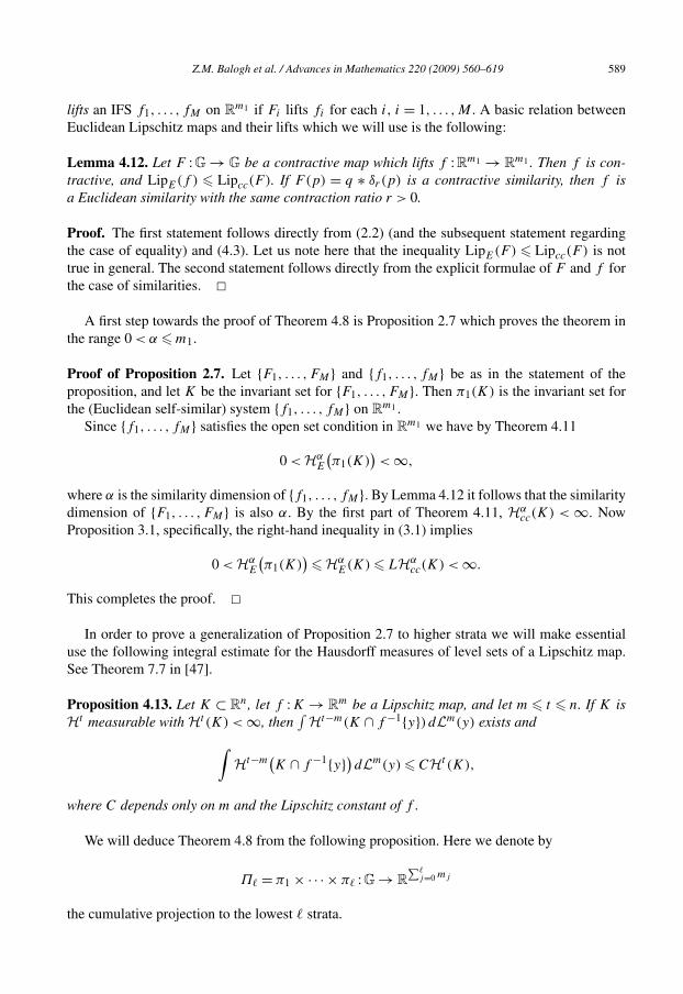
This completes the proof. �In order to prove a generalization of Proposition 2.7 to higher strata we will make essential

use the following integral estimate for the Hausdorff measures of level sets of a Lipschitz map.See Theorem 7.7 in [47].

Proposition 4.13. Let K ⊂ Rn, let f :K → Rm be a Lipschitz map, and let m � t � n. If K isHt measurable with Ht (K) < ∞, then

∫Ht−m(K ∩ f −1{y}) dLm(y) exists and∫

Ht−m(K ∩ f −1{y})dLm(y) � CHt (K),

where C depends only on m and the Lipschitz constant of f .

We will deduce Theorem 4.8 from the following proposition. Here we denote by

Π = π1 × · · · × π : G → R∑

j=0 mj

the cumulative projection to the lowest strata.


Proposition 4.14. Let G, be as in Theorem 4.8, b � 2 an integer, and M ∈ {1,2, . . . , b(+1)m+1}.For each j = 1, . . . , s, let Aj = {0, . . . , bj − 1}mj ⊂ Rmj . For a1 ∈ A1, . . . , ak ∈ Ak , let

pa1···ak= (a1, . . . , ak,0, . . . ,0)

and

Fa1···ak(p) = pa1···ak

∗ δ1/b

(p−1

a1···ak∗ p).

Finally, let B be any subset of A+1 of cardinality M , let

F = {Fa1···a+1 : a1 ∈ A1, . . . , a ∈ A, a+1 ∈ B},

and let K be the invariant set for the CC self-similar IFS F . Then

H∑

j=0 jmj + logMlogb

cc (K) < ∞ (4.15)

and

H∑

j=0 mj + logM

logb+1

E

(Π+1(K)

)> 0. (4.16)

Moreover, if M = b(+1)m+1 (in which case B = A+1), then H∑+1

j=0 mj

E -a.e. point X+1 ∈Π+1(K) has a unique symbolic representation

X+1 = Π+1

(lim

n→∞Fa11 ···a1

+1◦ · · · ◦ Fan

1 ···an+1

(o))

(4.17)

for some unique symbol sequence

σ = σ(X+1) = {((a11, . . . , a1

+1

),(a2

1, . . . , a2+1

), . . . ,

)} ∈ (A1 × · · · × A+1)N.

To simplify notation in what follows, we write

Fσ (o) = limn→∞Fa1

1 ···a1+1

◦ · · · ◦ Fan1 ···an

+1(o)

so that (4.17) reads

X+1 = Π+1(Fσ (o)

). (4.18)

Observe also that if

α =∑

mj + logM

logb+1∈[

∑mj ,

+1∑mj

](4.19)

j=0 j=0 j=0


is the exponent in (4.16), then

β−(α) =∑

j=0

jmj + logM

logb(4.20)

is the exponent in (4.15).

Proof of Theorem 4.8. Since Π+1 : (G, dE) → (R∑

j=0 mj , dE) is Lipschitz, Eqs. (4.15)and (4.16) guarantee the existence of a compact set S satisfying

HαE(S) > 0 (4.21)

and

Hβ−(α)cc (S) < ∞. (4.22)

in case α is of the form (4.19). An application of (2.8) together with the strict monotonicity of β−completes the proof in this case. The set of all such α, as b � 2 and M ∈ {1,2, . . . , b(+1)m+1}vary, is dense in the interval [∑

j=0 mj ,∑+1

j=0 mj ]. The case of general α follows from this andthe monotonicity and countable stability of the Hausdorff dimension.

The set S constructed as in the previous paragraph need not have topological dimension zero.However, since it necessarily has finite topological dimension (in fact, dimtop S � N ), we mayappeal to the decomposition theorem for topological dimension [36, Theorem III.3] to write S asthe union of a finite number of Borel subsets, each of topological dimension zero. Replacing S byan appropriately chosen one of these subsets yields a bounded Borel set of topological dimensionzero satisfying dimE S = α and dimcc S = β−(α). �Remark 4.15. For α as in (4.19) we can find a compact set S of topological dimension zerosatisfying (4.21) and (4.22). Indeed, for such α the subset described in the final sentence of theproof can be chosen satisfying (4.21) and (4.22). By a theorem of Howroyd (see [47, Chapter 8])there exists a further compact subset (necessarily of topological dimension zero) which alsosatisfies (4.21) and (4.22).

Proof of Proposition 4.14. The proof will be by induction on .Consider first the base case = 0. Let b � 2 and M ∈ {1, . . . , bm1}, let

A1 = {0, . . . , b − 1}m1 ⊂ Rm1,

pa1 = (a1,0, . . . ,0) ∈ G, a1 ∈ A1,

and consider the contractive similarity of (G, dcc) given by

Fa1(p) = pa1 ∗ δ1/b

(p−1

a1∗ p).

Let B ⊂ A1 be any set of cardinality M . The CC self-similar IFS F = {Fa: a ∈ B} has similaritydimension α = logM/ logb. Hence Hα

cc(K) < ∞ for the invariant set K . On the other hand,

Hα (K) � Hα(π1(K)

)
E E


and π1(K) is the invariant set for the Euclidean self-similar IFS F1 = {fa: a ∈ B}, fa(x) =a + 1

b(x − a), on Rm1 , which satisfies the open set condition with open set O1 = (0, b − 1)m1 .

Thus

HαE(K) > 0

as desired. If M = bm1 then Hm1E -a.e. x1 ∈ Π1(K) = π1(K) has a unique symbolic representation

relative to the IFS F (this is a consequence of the open set condition). This completes the proofin the case = 0.

Now assume that the statement in the proposition is true for some integer −1 and all integersb0 � 2 and M0 ∈ {1,2, . . . , bm}; we will prove that it holds true for and any given pair ofintegers b � 2 and M ∈ {1,2, . . . , b(+1)m+1}. Let b and M be given. According to the inductivehypothesis in the ( − 1)st step with b0 = b and M0 = b

m

0 , the invariant set K0 for the CCself-similar IFS

F0 = {Fa1···a: a1 ∈ A1, . . . , a ∈ A},

satisfies the estimates

H∑

j=0 jmj

cc (K0) < ∞ (4.23)

and

H∑

j=0 mj

E

(Πl(K0)

)> 0, (4.24)

furthermore, almost every point X ∈ Π(K0) has a unique symbolic representation.Now let B be any subset of A+1 of cardinality M , let F be the CC self-similar IFS comprised

of the mappings Fa1···a+1 for a1 ∈ A1, . . . , a ∈ A and a+1 ∈ B , and let K be the invariant setfor F . Note that

Π(K0) ⊆ Π(K). (4.25)

We will prove that (4.15) and (4.16) hold. The former follows immediately from the fact that Fis CC self-similar with similarity dimension

log(b∑

j=0 jmj M)

logb= β−(α);

see (4.20).To prove the latter, we will apply Proposition 4.13 with t = α as in (4.19), m =∑l

j=0 mj andf = Π. We have to show that there exists a constant c > 0 so that

Hα−∑j=0 mj

E

(K ∩ Π−1

(X))� c (4.26)

for almost every Xl ∈ Πl(K).In view of (4.24) and (4.25), Proposition 4.13 yields (4.22).To prove (4.26) we begin with a lemma.


Lemma 4.16. Let πq : G → Rmq denote projection to the qth stratum, q = + 1. For every X ∈Π(K) which has a unique symbolic representation, the set πq(K ∩ Π−1

(X)) is a Euclideantranslate of the invariant set K ′ ⊂ Rmq of the Euclidean self-similar IFS

G = {gaq : aq ∈ B}, (4.27)

where ga(x) = 1bq x + (1 − 1

bq )a.

We emphasize that in Lemma 4.16 the translation parameter depends on X = (x1, . . . , x),but the IFS G does not.

Proof of Lemma 4.16. Let X be as in the statement and let σ = σ(X) ∈ (A1 × · · · × A)N be

the unique associated symbol string. In the remainder of this proof, we use x′ = (x′1, . . . , x

′s) for

a dummy variable in G, as well as our standard notation X′ = (x′

1, . . . , x′).

Let us first consider the expression

πq ◦ Fa1···aq (x′) −

[1

bqxq +

(1 − 1

bq

)aq

](4.28)

as a function of x′ ∈ K and (a1, . . . , aq). From the form of the Baker–Campbell–Hausdorff for-mula (see especially (4.3)) we conclude that the expression in (4.28) is independent of x′

q and aq ,i.e., depends only on X′

and (a1, . . . , a). We write

πq ◦ Fa1···aq (x′) = 1

bqx′q +

(1 − 1

bq

)aq + Φ1

(X′

;a1, . . . , a

)(4.29)

for some real-valued function Φ1 defined on Π(K) × (A1 × · · · × A).Similarly, for any n, the expression

πq ◦ Fa11 ···a1

q◦ · · · ◦ Fan

1 ···anq(x) −

[n∑

m=1

1

bq(m−1)

(1 − 1

bq

)amq + 1

bqnx′q

], (4.30)

considered as a function of x′ ∈ K and (a11, . . . , a1

q), . . . , (an1 , . . . , an

q ) is independent of x′q and

a1q, . . . , an

q , i.e., depends only on X′ and (a1

1, . . . , a1 ), . . . , (a

n1 , . . . , an

). We write

πq ◦ Fa11 ···a1

q◦ · · · ◦ Fan

1 ···anq(x′)

= 1

bqnxq +

n∑m=1

1

bq(m−1)

(1 − 1

bq

)amq + Φn

(X′

;(a1

1, . . . , a1

), . . . ,

(an

1 , . . . , an

))(4.31)

for some real-valued function Φn defined on Π(K) × (A1 × · · · × A)n.

This behavior passes to the limit as n → ∞, where we conclude that

πq ◦ Fσ (x′) =∞∑ 1

bq(m−1)

(1 − 1

bq

)amq + Φ∞

(X′

, σ)

(4.32)
m=1


for some real-valued function Φ∞ defined on Π(K) × (A1 × · · · × A)N. Since σ = σ(X) is

uniquely determined by X, we can write (4.32) as

πq ◦ Fσ (x′) =∞∑

m=1

1

bq(m−1)

(1 − 1

bq

)amq + Φ∞

(X′

, σ (X)). (4.33)

Next, we observe that xq is in πq(K ∩ Π−1 (X)) if and only if there exists a symbol string

σ ∈ (A1 × · · · × A × B)N so that xq = πq(Fσ (o)). By (4.33) this means

xq =∞∑

m=1

1

bq(m−1)

(1 − 1

bq

)amq + Φ∞

((0, . . . ,0), σ (X)

)(4.34)

for a suitable choice of (a1q, a2

q, . . .) ∈ BN. Set R(X) = Φ∞((0, . . . ,0), σ (X)). Eq. (4.34) holds

for some sequence (a1q, a2

q, . . .) ∈ BN if and only if xq ∈ K ′ + R(X). Thus

πq

(K ∩ Π−1

(X))= K ′ + R(X).

This completes the proof of the lemma. �With this proof in hand we now quickly complete the proof of the proposition. The IFS G

in (4.27) satisfies the open set condition (use the open set O = (0, bq − 1)mq ) and has similaritydimension logM/ logbq = α −∑

j=0 mj , see (4.19). Thus

Hα−∑j=0 mj

E

(K ∩ Π−1

(X))� Hα−∑

j=0 mj

E

(πq

(K ∩ Π−1

(X)))= HlogM/ logbq

E (K ′) > 0

for almost every X ∈ Π(K). This completes the proof of (4.26) and hence also the proofof (4.16). Moreover, the identity in (4.34) shows that each point in Πq(K ∩ Π−1

(X)) has a

unique symbolic representative, provided that X and also xq do. If M = bqmq , H∑q

j=0 mj

E -a.e.point in Πq(K) is of this type, by Fubini’s theorem. This completes the proof of Proposi-tion 4.14. �Remark 4.17. The set S in Theorem 4.8 has well-defined Euclidean and CC box-counting di-mensions, and dimB

cc S = β−(dimBE S). Indeed, as a CC self-similar set, S necessarily satisfies

dimBcc S = dimH

cc S = β−(α). Moreover,

dimB

E S � (β−)−1(dimBcc S)= α = dimH

E S � dimBE S

which shows that the Euclidean box-counting dimension of S exists and equals α.

Remark 4.18. We reiterate the purely Euclidean consequences of Theorem 4.8. The CC self-similar iterated function systems constructed in Proposition 4.14 can be viewed as iteratedfunction systems in the underlying Euclidean geometry; in view of the nilpotence of G andthe Baker–Campbell–Hausdorff formula the associated mappings are polynomial of an a priorihigh degree. Thus, viewed in Euclidean terms, these IFS are nonlinear and nonconformal; it is


typically quite difficult to calculate explicitly the dimensions of such systems by traditional meth-ods. Nevertheless, by our approach we obtain an explicit formula for their Euclidean Hausdorffdimension. As an illustration, we restate Example 2.10 in purely Euclidean terms. Consider thefour maps of R4 given by

F1(x) =(

1

2x1,

1

2x2,

1

4x3,

1

8x4

), (4.35)

F2(x) =(

1

2x1 + 1

2,

1

2x2,

1

4x3,

1

8x4

), (4.36)

F3(x) =(

1

2x1,

1

2x2 + 1

2,

1

4x3 + 1

4x1,

1

8x4 + 3

16x2

1

), (4.37)

and

F4(x) =(

1

2x1 + 1

2,

1

2x2 + 1

2,

1

4x3 + 1

4(x1 − 1),

1

8x4 + 1

16(x1 − 1)2

), (4.38)

where x = (x1, x2, x3, x4). These are evidently not global contractive maps of (R4, dE). How-ever, since they are precisely the contractive similarities of the Carnot Engel group specified inExample 2.2, we know that they generate a compact invariant set in R4 whose Euclidean Haus-dorff dimension is exactly equal to 2. (See Section 2 for pictures of some three-dimensionalprojections of this set.)

Remark 4.19. We conclude this section by discussing the implications of Theorems 2.4 and 2.6for the theory of codimension one horizontal rectifiability as developed by Franchi, Serapioni andSerra Cassano [27,26]. Let G be a Carnot group. We recall the following definitions from [26]:

(i) u : G → R is a C1G

function if Xu is continuous for all X ∈ V1,(ii) the horizontal gradient of a C1

Gfunction u : G → R is the unique map ∇Gu : G → V1 satis-

fying Xu = 〈X,∇Gu〉 for all X ∈ V1,(iii) a codimension one hypersurface S is G-regular if it is locally the zero set of a C1

Gfunction

with nonvanishing horizontal gradient,(iv) a set S in G is called horizontally (Q − 1)-rectifiable (or horizontally rectifiable in codi-

mension one) if S is the union of a countable family of G-regular hypersurfaces, togetherwith a set of HQ−1

cc -dimensional measure zero.

We say that S ⊂ G is k-rectifiable, 0 � k � N , if it is rectifiable in the classical Euclidean senseas a subset of RN : S is the union of a countable family of Lipschitz images of subsets of Rk ,together with a set of Hk

E-dimensional measure zero.It is of interest to understand the difference between notions of Euclidean (N −1)-rectifiability

and the horizontal codimension one rectifiability of subsets of G with underlying space RN . Thefollowing corollary to Theorem 2.6 extends [5, Theorem 5.1] to the setting of general Carnotgroups.


Corollary 4.20. Let G be a Carnot group of dimension N and homogeneous dimension Q. Thenevery (N −1)-rectifiable set in G is horizontally (Q−1)-rectifiable. In every nonabelian Carnotgroup, there exist horizontally (Q − 1)-rectifiable sets S ⊂ G which are not (N − 1)-rectifiable.

Proof. Let S ⊂ G = RN be (N − 1)-rectifiable. By standard Euclidean geometric measure the-ory, S = Z ∪⋃∞

i=1 Si , where Si is the zero set of a C1 function fi : RN → R and HN−1E (Z) = 0.

We denote by C(Si) the characteristic set of the hypersurface Si , i.e., the set of points x ∈ Si forwhich HxG ⊂ TxSi . The complement of C(Si) in Si is the subset of {fi = 0} on which ∇Gfi �= 0.By [43, Theorem 6.6.2], HQ−1

cc (C(Si)) = 0. By Proposition 3.1, HQ−1cc (Z) = 0. We have

S =(

Z ∪∞⋃i=1

C(Si)

)∪

∞⋃i=1

(Si \ C(Si)

)= Z′ ∪∞⋃i=1

S′i ,

where HQ−1cc (Z′) = 0 and S′

i is a G-regular hypersurface. Thus S is horizontally (Q − 1)-rectifiable.

To construct a set S in a nonabelian Carnot group G as in the second assertion, observe that(β−)−1(Q − 1) = N − s−1, where s is the step of the group. Since G is nonabelian, s � 2.We may choose a pair of monotone increasing sequences (αν) and (βν) satisfying N − 1 < α1,limν→∞ αν = N − s−1, and βν = β−(αν). With Sα,β the set constructed in Theorem 2.6, we have

S =∞⋃

ν=1

Sαν,βν

satisfies HQ−1cc (S) = 0 (so S is trivially horizontally (Q − 1)-rectifiable) but dimE S � α1 >

N − 1. In fact we have that dimE S = N − s−1 and so S is not (N − 1)-rectifiable. �Kirchheim and Serra Cassano [40] have constructed an H1-regular hypersurface in H1 whose

Euclidean Hausdorff dimension is 2.5, even locally at every point. Note that 2.5 = (βH1

− )−1(3). Inany Carnot group G, does there exist a G-regular hypersurface of Euclidean dimension N − s−1?

5. CC self-similar invariant sets in Carnot groups are almost surely horizontal

This section is devoted to the proof of Theorem 2.8, which establishes the equality

dimcc K = β−(dimE K)

almost surely for generic members of certain finite-dimensional parameterized families of CCself-similar sets K in a Carnot group G. Inspiration for this type of result comes from work ofFalconer [20,22], which establishes similar results for generic members of certain families ofself-affine invariant sets in Euclidean space. In view of the fact that the group operation in G

is given by polynomial maps, our results return purely Euclidean dividends: we obtain almostsure dimension statements for families of nonlinear, nonconformal Euclidean invariant sets. Inthe following section, we illustrate this point in the jet space Carnot groups.


Let us begin by briefly recalling the work of Falconer [20]. The singular value function ofa contractive linear map A : Rn → Rn is defined as

ϕt (A) ={1, t = 0,

μ1μ2 · · ·μm−1μt−m+1m , m − 1 < t � m,

(μ1 · · ·μn)t/n, t � n,

where 1 > μ1 � μ2 � · · · � μn � 0 denote the singular values of A, i.e., the positive square rootsof the eigenvalues of A∗A. The operator norm of A is the largest eigenvalue ‖A‖ = μ1.

Next, let A = {A1, . . . ,AM} be a finite collection of contractive linear maps. Then for anyt � 0 the limit

limm→∞

( ∑w: |w|=k

ϕt (Aw)

)1/m

(5.1)

exists, where the sum is taken over all words w = w1w2 · · ·wm of length m in the letters{1,2, . . . ,M} and Aw = Aw1 · · ·Awm . (For a more complete review of the symbolic dynamicsof iterated function systems, see Subsection 5.1.) The expression in (5.1) is a strictly decreasing,continuous function of t , and we let

d(A) = the unique nonnegative value of t such

that the quantity in (5.1) is equal to one. (5.2)

Falconer [20] proved Theorem 5.1 with ‖Ai‖ < 13 for all i; the stated generalization is due to

Solomyak [57].

Theorem 5.1 (Falconer, Solomyak). Assume that ‖Ai‖ < 12 for all i = 1, . . . ,M . Then, for almost

every b = (b1, . . . , bM) ∈ Rn×M , we have

dimE K(b) = min{d(A), n

},

where K(b) denotes the invariant set for the affine IFS {F1, . . . ,FM}, Fi(x) = Aix + bi .

Theorem 5.1 has been generalized to the setting of horizontal self-affine IFS in the firstHeisenberg group by the first two authors in [7] (see also [4]). The purpose of this section isto prove Theorem 2.8 which provides a far-reaching generalization of Falconer’s almost sure di-mension result to the setting of horizontal self-similar IFS in general Carnot groups. A furthergeneralization to horizontal self-affine Carnot IFS is presumably possible, but we do not addressthis here.

As will be explained in more detail in the following section, the transition formula

α = (β−)−1(β)

in (2.10), which arises from the lower dimension comparison statement in Theorem 2.4, encodesthe same information as Falconer’s formulas (5.1) and (5.2) in the setting of jet space groups.


5.1. Symbolic dynamics and iterated function systems

In this subsection, we recall the formalism of symbolic dynamics in the context of iteratedfunction systems. Our notation follows [39]. Let F = {F1, . . . ,FM} be a self-similar IFS on acomplete metric space (X,d), and denote by ri the contraction ratio associated to Fi . For k � 1,define

Wk := {1, . . . ,M}k = {w1 · · ·wk: wm ∈ {1, . . . ,M}, 1 � m � k},

called the set of words of length k in the alphabet {1, . . . ,M}. For k = 0, set W0 = {∅} and call ∅the empty word. Finally, define

W∗ =∞⋃

k=0

Wk

to be the set of finite sequences and

Σ = {w1w2 · · · : wm ∈ W1}

the set of infinite sequences.We write vw for the concatenation of two words v,w ∈ W∗: vw = v1v2 · · ·vkw1w2 · · ·wl if

v = v1 · · ·vk ∈ Wk and w = w1 · · ·wl ∈ Wl . If w = vv′ for some word v′ we say that v is a sub-word of w. The largest common subword of v and w will be denoted v ∧ w; this is characterizedas the unique common subword of v and w which is maximal with respect to length. We willabuse notation slightly, denoting by w both finite and infinite words.

For S ⊂ X and w = w1 · · ·wk ∈ W∗, define Fw = Fw1 ◦ · · · ◦ Fwk, rw = rw1 · · · rwk

, andSw = Fw(S).

We equip Σ with the product topology induced by the discrete topology on the alphabet. Thenthere exists a canonical continuous surjection π :Σ → K to the invariant set of F , characterizedby the relation {π(w)} =⋂∞

k=1 Fw1···wk(K). Alternatively,

π(w) = limk→∞Fw1···wk

(x0)

for any fixed x0 ∈ X. The map π is called the canonical symbol map for the IFS {F1, . . . ,FM}.We record the commutation relation

π ◦ σw = Fw ◦ π, w ∈ W∗, (5.3)

where σ :Σ → Σ denotes the left shift,

σ(w1w2w3 · · ·) = w2w3 · · · ,

and σw :Σ → Σ the map which prepends w to its argument,

σw(v) = wv.


The cylinder set over w ∈ W∗ is Σw = σw(Σ); this set consists of all infinite words which beginwith w. By (5.3), π(Σw) = Kw . A partition of Σ is a disjoint collection of cylinder sets whichcovers Σ .

5.2. Proof of Theorem 2.8

The proof of Theorem 2.8 uses energy estimates to obtain almost sure lower bounds on Haus-dorff dimension. We recall the following standard result, see, for example Theorems 4.2 and 4.13in [21] or Theorem 8.7 in [47].

Proposition 5.2. Let S be a subset of a complete metric space (X,d) and let μ be a positive andfinite Borel regular measure supported on S whose s-energy∫

X

∫X

d(x, y)−s dμ(x)dμ(y)

is finite. Then the Hausdorff dimension of S is at least s.

Assume that F is a self-similar IFS as above, and let t � 0 be the similarity dimension for F .Following Kigami [39], we introduce a probability measure λ on the symbol space Σ as follows:

λ(E) = limm→∞ inf

Λ

∑w∈Λ

E∩Σw �=∅

rtw, (5.4)

where the infimum is taken over all partitions Λ of Σ into cylinder sets defined by words oflength at least m. Note that

λ(Σw) = rtw (5.5)

for cylinder sets Σw , indeed,∑

v∈Λ: Σw∩Σv �=∅ rtv = rt

w if Λ partitions by words of length atleast |w|.

Let us recall the notations for r, P, α(r), β(r) introduced before the statement of Theorem 2.8.In our proofs below we shall consider the measure λ for the value t = β(r) and we emphasizeon the fact that λ depends only on r and not on P. We will use λ in this connection for invariantsets K(P) where P varies but r is fixed. Furthermore, for P ∈ GM we denote the canonicalsymbol map by πP :Σ → K(P). An essential ingredient in the proof of Theorem 2.8 is thefollowing statement.

Proposition 5.3. Let G and r be as in Theorem 2.8, and define α = α(r) and β = β(r) as before.For each 0 < R < ∞ and α′ < α,∫

B(R)M

∫Σ

∫Σ

∣∣πP(u) − πP(v)∣∣−α′E

dλ(u)dλ(v) dP < ∞, (5.6)

where B(R) denotes the (Euclidean) ball of radius R in G centered at o ∈ G, dP denotes theelement of integration with respect to the M-fold product of Haar measures on GM , and dλ isthe measure defined in (5.4) with t = β .


Proof of Theorem 2.8. As discussed in Section 2, to prove the Hausdorff dimension statementsin Theorem 2.8 it suffices to prove the inequality

dimE K(P) � α

for almost every P ∈ GM . For each 0 < R < ∞, we obtain from (5.6) that∫Σ

∫Σ

∣∣πP(u) − πP(v)∣∣−α′E

dλ(u)dλ(v) < ∞

for almost every P ∈ B(R)M , hence∫K(P)

∫K(P)

|p − q|−α′E d

((πP)#λ

)(p)d

((πP)#λ

)(q) < ∞

where the integration is with respect to the pushforward measure (πP)#λ. By Proposition 5.2,dimE K(P) � α′ for every such P. Letting α′ → α and R → ∞ completes the proof in theHausdorff dimension case. The box-counting dimension case follows once we observe that con-dition (a) for upper box-counting dimension holds by the general theory of iterated functionsystems. �

We derive Proposition 5.3 from the following technical lemma which is at the heart of theproof.

Lemma 5.4. Assume that γ := max{r1, . . . , rM} < 12 . For each R < ∞ and 0 � s � N , there

exists a constant C = C(R,G, α, γ ) so that∫B(R)M

∣∣πP(v)−1 ∗ πP(u)∣∣−α

EdP � C

rβ−(α)u∧v

(5.7)

for all u,v ∈ Σ .

Proof of Proposition 5.3. Let β ′ = β−(α′). Recall that β is defined as in (2.9). By monotonicityof β−, β > β ′. Using Fubini’s theorem, (5.7), (3.3) and (5.5), we estimate the integral in (5.6) asfollows: ∫

B(R)M

∫Σ

∫Σ

∣∣πP(u) − πP(v)∣∣−α′E

dλ(u)dλ(v) dP

�∫

B(R)M

∫Σ

∫Σ

∣∣πP(v)−1 ∗ πP(u)∣∣−α′E

dλ(u)dλ(v) dP

� C(R,G, α′)∫ ∫

r−β ′u∧v dλ(u)dλ(v)

Σ Σ


= C(R,G, α′)∑

w∈W∗

∑i �=j

r−β ′w λ(Σwi)λ(Σwj )

� C(R,G, α′)∑

w∈W∗rβ−β ′w λ(Σw) � C(R,G, α′)

∞∑m=1

2−m(β−β ′) ∑w∈Wm

λ(Σw).

The latter expression is finite since∑

w∈Wmλ(Σw) = 1 and β > β ′. �

In the proof of Lemma 5.4 we will make use of the following explicit representation for thesymbolic representation map πP :Σ → K(P): if u = u1u2 · · ·um · · · ∈ Σ , then

πP(u) = limm→∞Fu1 ◦ · · · ◦ Fum(o)

= limm→∞pu1 ∗ δru1

(pu2 ∗ δru2

(pu3 ∗ · · · ∗ (pum ∗ δrum

(o))))

= limm→∞pu1 ∗ δru1

pu2 ∗ δru1 ru2pu3 ∗ · · · ∗ δru1 ···rum−1

pum. (5.8)

Proof of Lemma 5.4. Let 0 < R < ∞ and 0 � s � N . By the Ball–Box Theorem, it suffices toverify (5.7) with the region of integration replaced by the M-fold product of CC balls Bcc(R)M .

Using the notation |x|cc = dcc(x,0) let us observe that if P ∈ Bcc(0,R), then (5.8) and itera-tions of the triangle inequality for dcc imply that∣∣πP(u)

∣∣cc

� |pu1 |cc + ru1 |pu2 |cc + ru1ru2 |pu3 |cc + · · ·

� R + 1

2R + 1

4R + · · · = 2R, (5.9)

hence

πP(u) ∈ Bcc(0,2R)

for all u ∈ Σ and P ∈ Bcc(R).Now let u,v ∈ Σ , let w = u ∧ v, and assume that |w| = k. Since the maps Fj are CC similar-

ities,

dcc

(πP(u),πP(v)

)= rwdcc

(πP(σku

),πP(σkv

))� 4Rrw

by (5.9), so

πP(v)−1 ∗ πP(u) ∈ Bcc(0,4Rrw).

By the Ball–Box Theorem, we conclude that[πP(v)−1 ∗ πP(u)

]j

∈ Boxmj

E

((C′rw)j

), (5.10)

where C′ depends only on R and CBB and the Euclidean box in (5.10) is taken in Rmj .Next, we record a useful explicit representation for the j th stratum of πP(v)−1 ∗ πP(u). Re-

call that P = (p1, . . . , pM). We write pi ∈ G in exponential coordinates: pi = (pi1, . . . , pis)


where pij ∈ Rmj for j = 1, . . . , s. Without loss of generality, we may assume that uk+1 = 1 andvk+1 = 2.

From (5.8) and (4.3) we find[πP(v)−1 ∗ πP(u)

]j

= rjw

(p1j − p2j +

∞∑m=k+2

rj

1 rjuk+2 · · · rj

um−1pum,j − rj

2 rjvk+2

· · · rjvm−1

pvm,j

)+ Θj(P1,j−1, . . . ,PM,j−1)

= rjw

(p1j − p2j +

M∑i=1

Eij (pij )

)+ Θj(P1,j−1, . . . ,PM,j−1), (5.11)

where Θj is a real analytic function in the lower strata variables P1,j−1, . . . ,PM,j−1 andE1j , . . . ,EMj : Rmj → Rmj are linear maps. In fact, each Eij is just a standard Euclidean dilationof Rmj . Here we have used the notation from (4.2) for the cumulative lower strata variables Pij

associated to pi ∈ G. An explicit computation using (5.11) shows that

Eij (xj ) = ρjxj , xj ∈ Rmj , (5.12)

where ρj is the sum over m ∈ N of terms of the form εm,1rjηm,1 + εm,2r

jηm,2 with ηm,1, ηm,2 ∈ Wm

and (εm,1, εm,2) ∈ {(0,0), (+1,0), (0,−1), (+1,−1)}. Note that ηm,i and εm,i , i = 1,2 (hencealso ρj and Eij ) depend on u and v; see the middle expression in (5.11) for the explicit formula.For simplicity, we omit mention of this dependence in the notation.

The following argument is inspired by Falconer [20]. Our goal is to show that for each0 � l � s − 1 the change of variables P → P defined by

p1j �→{

qj := [πP(v)−1 ∗ πP(u)]j , j = 1, . . . , l + 1,

p1j , j = l + 2, . . . , s,

pij �→ pij , i = 2, . . . ,M, j = 1, . . . , s, (5.13)

is invertible.Since ri � γ < 1

2 for all i and j � 1, (5.12) yields

‖Eij‖ = |ρj | �∞∑

m=1

max{|εm,1|, |εm,2|

}γ jm �

∞∑m=1

γ jm = γ j

1 − γ j< 1

for each i, thus Eij is a strict contraction and I + E1j is invertible with

∥∥(I + E1j )−1∥∥� 1 − γ j

1 − 2γ j. (5.14)

Using the lower triangular form of (5.11) it follows that the change of variables (5.13) is invert-ible. We compute its Jacobian determinant as:

dqj = rjmjw det(I + E1j ) dp1j (5.15)


and observe that

det((I + E1j )

−1)� ∥∥(I + E1j )−1∥∥mj �

(1 − γ j

1 − 2γ j

)mj

(5.16)

by Hadamard’s inequality and (5.14).Finally, we estimate

I :=∫

Bcc(R)M

∣∣πP(v)−1 ∗ πP(u)∣∣−α

EdP. (5.17)

We fix = (α) ∈ {0, . . . , s − 1} as in (2.5): l is the unique integer satisfying∑

j=0 mj < α �∑+1j=0 mj . We bound the integrand in (5.17) from above by

∣∣([πP(v)−1 ∗ πP(u)]

1, . . . ,[πP(v)−1 ∗ πP(u)

]+1

)∣∣−α

E.

Making the preceding change of variables and using (5.10), (5.15) and (5.16), we conclude that

I � C(R,G, γ )r−∑+1

j=0 jmj

w ×∫

Boxm1E (C′rw)

· · ·∫

Boxm+1E ((C′rw)l+1)

∣∣(q1, . . . , q+1)∣∣−α

Edq+1 · · ·dq1

or more simply,

I � C(R,G, γ )r−∑+1

j=0 jmj

w

∫Π+1 Boxcc(C′rw)

|Q+1|−αE dQ+1.

To conclude the proof, we write

Π+1 Boxcc(C′rw) =

⋃σ⊂S

Aσ ,

where the union is taken over all nonempty subsets σ of S = {1, . . . , + 1} and Aσ denotes theset of points Q+1 = (q1, . . . , q+1) in Π+1 Boxcc(C

′rw) for which |qj | � (C′rw)+1 for allj ∈ σ . Then ∫

AS

|Q+1|−αE dQ+1 �

∫B

∑+1j=0 mj

E (√

N(C′rw)+1)

|Q+1|−αE dQ+1

and ∫Aσ

|Q+1|−αE dQ+1 � (C′rw)

∑j∈S\σ jmj

∫R

∑j∈σ mj \B

∑j∈σ mj

((C′r )+1)

|Qσ |−αE dQσ

E w


for σ = {σ1, . . . , σ#σ } � S (with obvious notation Qσ = (qσ1, . . . , qσ#σ )). In either case we obtain∫Aσ

|Q+1|−αE dQ+1 � C(R,G, α)r

(+1)(∑+1

j=1 mj −α)

w ;

summing over all nonempty subsets of S yields

I � C(R,G, α, γ )r−∑+1

j=0 jmj

w r(+1)(

∑+1j=0 mj −α)

w = C(R,G, α, γ )r−β−(α)w .

This completes the proof of Lemma 5.4. �6. Jet spaces

Our goal in this section is twofold. First, we illustrate the main results of this paper in a well-known explicit class of Carnot groups: the jet spaces J k(R,R). In the standard Carnot grouppresentation of J k(R,R), similarity maps are polynomial in the underlying Euclidean geometry.

In the second part of the section we describe an alternate Carnot group presentation ofJ k(R,R) in which similarities are affine maps in the Euclidean geometry and the constituentlinear maps are given by triangular matrices. We then relate our work to that of Falconer andMiao in [18].

6.1. Jet spaces as Carnot groups: the classical model

References for this material include Section 6.4 in [50, §6.4], [61] and [62]. General discus-sions of the geometry of jet spaces and jet bundles can be found in [54] and [56].

The kth order Taylor polynomial of a Ck function f : R → R at a point x0 ∈ R is

(T k

x0f)(ξ) =

k∑i=0

f(i)(x0)(ξ − x0)

i

i! .

Two functions f1, f2 ∈ Ck(R) are defined to be equivalent at x0, written f1 ∼x0 f2, if T kx0

f1 =T k

x0f2. The equivalence class of f is the k-jet of f at x0, denoted jetkx0

(f). The kth order jet spaceis

J k(R,R) :=⋃

x0∈R

Ck(R)/∼x0 .

We identify J k(R,R) with the Euclidean space Rk+2 by introducing coordinates x :J k(R,R) →R and uj :J k(R,R) → R, 0 � j � k, where x(jetkx0

(f)) = x0 and uj (jetkx0(f)) = f(j)(x0). In this

coordinate system we will write elements of J k(R,R) as (k + 2)-tuples

p = (x,u(k))= (x,uk, . . . , u0).

Contact and horizontal structures in J k(R,R)J k(R,R)J k(R,R). The k-jet of a map f ∈ Ck(R) is the sectionx0 �→ jetk (f) of the bundle x :J k(R,R) → R. A contact form θ on J k(R,R) is a 1-form satis-
x0


fying (jetk•(f))∗θ = 0 for all k-jets jetk•(f). By the chain rule, the cotangent space is framed by thecollection of 1-forms dx, ωk = duk , and ωj = duj − uj+1dx where j = 0, . . . , k − 1.

The horizontal tangent bundle H is defined pointwise by

Hp = {V ∈ TpJ k(R,R): ωj (V ) = 0 for all j = 0, . . . , k − 1}.

In coordinates, V = dx(V )X +ωk(V )Uk , where X = ∂∂x

+uk∂

∂uk−1+· · ·+u1

∂∂u0

and Uj = ∂∂uj

for j = 0, . . . , k. We note the nontrivial commutation relations

[Uj ,X] = Uj−1, j = 1, . . . , k. (6.1)

Setting V1 = H = span{X,Uk} and Vj = span{Uk−j+1} = [V1,Vj−1] for j = 2, . . . , k + 1, weobtain a (k +1)-step nilpotent Lie algebra jk = jk(R,R) = v1 ⊕· · ·⊕vk+1 which gives J k(R,R)

the structure of a (k + 1)-step Carnot group.The homogeneous dimension of J k(R,R) is Q = 1 + (k+2

2

)while the underlying Euclidean

space is Rk+2. The bases {X,Uk, . . . ,U0} and {dx,ωk, . . . ,ω0} are dual. Note that it is the vectorfields X and Uk which define the horizontal directions in this presentation.

Remark 6.1. j1 is isomorphic to the Lie algebra of the first Heisenberg group, and j2 is isomor-phic to the Lie algebra of the Engel group. In general, jk is known as the kth Goursat algebra ormodel filiform algebra. It arises naturally in control theory as the configuration space for optimalpath planning in the kinematics of multi-stage trailers, cf. [48].

The group law, dilations and similarities in J k(R,R)J k(R,R)J k(R,R). Using the above introduced, so-calledsecond kind coordinates, the group law reads as follows:(

x,u(k))� (y, v(k)

)= (z,w(k)),

where z = x + y and

wj = vj +k∑

l=j

ul

yl−j

(l − j)! , 0 � j � k. (6.2)

The dilation of J k(R,R) by scaling factor r is

δr

(x,u(k)

)= (rx, ruk, r2uk−1, . . . , r

k+1u0). (6.3)

From (6.2) it follows that similarities in J k(R,R) are given by polynomials of degree k + 1 inthis model.

In the setting of J k(R,R), Theorems 2.4 and 2.6 read as follows.

Theorem 6.2. For S ⊂ J k(R,R), β−(dimE(S)) � dimcc(S) � β+(dimE(S)), where the upperdimension comparison function for J k(R,R) is

β+(α) ={

(k − l + 1)α + (l+12

), α ∈ [l, l + 1], l = 0, . . . , k − 1,

α + (k+1), α ∈ [k, k + 2], (6.4)

2


and the lower dimension comparison function for J k(R,R) is

β−(α) ={

α, α ∈ [0,2],(l + 1)α + 1 − (l+2

2

), α ∈ [l + 1, l + 2], l = 1, . . . , k.

(6.5)

6.2. Jet spaces as Carnot groups: an alternate model

We now describe another Carnot group model for the jet space J k(R,R). The principal ad-vantage of this model, in the context of this paper, is that left translation is given by affine mapsin the underlying Euclidean geometry. Thus CC self-similar IFSs are Euclidean self-affine. Thisgives us the possibility to compare our results with the recent work of Falconer and Miao in [18].

In this model, we identify J k(R,R) with Rk+2 by introducing a different set of coordinates:x :J k(R,R) → R and uj :J k(R,R) → R, 0 � j � k, where x(jetkx0

(f)) = x0 and

uj

(jetkx0

(f))= ∂

∂ξj

(T k

x0f)(ξ)∣∣ξ=0 =

k∑i=j

f (i)(x0)(−x0)

i−j

(i − j)! . (6.6)

In these coordinates we will write elements of J k(R,R) as (k + 2)-tuples p = (x, u(k)) =(x, uk, . . . , u0). We obtain from (6.6) the coordinate transformation φ(x,u(k)) = (x, u(k)), where

uj =k∑

i=j

ui

(−x)i

i! ,

which converts between the two models. Indeed, we define the group law so that φ becomes anisomorphism, setting(

x, u(k)) ∗ (y, v(k)

)= φ(φ−1(x, u(k)

)� φ−1(y, v(k)))= (x + y, w(k)

)and

wj = uj +k∑

l=j

vl

(−x)l−j

(l − j)! , 0 � j � k.

It now follows that the left invariant vector fields are given by

X = ∂

∂xand Uj = ∂

∂uj

− x∂

∂uj−1+ · · · + 1

j ! (−x)j∂

∂u0,

where 0 � j � k, and we observe that these vector fields satisfy the nontrivial commutationrelations

[Uj , X] = Uj−1, j = 1, . . . , k. (6.7)


Thus jk(R,R) = v1 ⊕ · · · ⊕ vk+1 where v1, . . . ,vk+1 correspond to the vector bundles V1 =span{X, Uk} and Vj = span{Uk−j+1} for j = 2, . . . , k. The dual forms are dx, duk , ωk−1, . . . , ω0where

ωj =k∑

=j

x−j

( − j)! du

for j = 0, . . . , k − 1. In this model the dilation by scaling factor r is

δr

(x, u(k)

)= (rx, ruk, r2uk−1, . . . , r

k+1u0). (6.8)

We emphasize again the crucial feature of this model: left translation (y, v(k)) → (x, u(k)) ∗(y, v(k)) is an affine map of the underlying Euclidean space Rk+2. With dilations δr defined asin (6.8), we see that the CC similarity(

z, w(k))= F

(x, u(k)

)= (a, b(k)) ∗ δr

(x, u(k)

),

for fixed p0 = (a, b(k)) ∈ J k(R,R), takes the form z = rx + a and

wj =k∑

l=j

rk+1−l ul

(−a)l−j

(l − j)! + bj

for 0 � j � k. Observe that F is a Euclidean affine map of the form

⎛⎜⎜⎜⎜⎝z

wk...

w1w0

⎞⎟⎟⎟⎟⎠=

⎛⎜⎜⎜⎜⎜⎜⎜⎝

r

0 r

0 −ra r2

......

. . .. . .

0 r(−a)k−1

(k−1)! · · · −rk−1a rk

0 r(−a)k

k! · · · rk−1a2

2 −rka rk+1

⎞⎟⎟⎟⎟⎟⎟⎟⎠

⎛⎜⎜⎜⎜⎝x

uk...

u1u0

⎞⎟⎟⎟⎟⎠+

⎛⎜⎜⎜⎜⎝a

bk...

b1b0

⎞⎟⎟⎟⎟⎠ . (6.9)

6.3. A relation between self-similar sub-Riemannian fractal geometry and self-affine Euclideanfractal geometry in jet spaces

Let us recall that Theorem 5.1 of Falconer gives an explicit expression for the almost suredimension of the invariant sets of Euclidean self-affine iterated function systems which involvestaking a limit of an average of the singular value functions of iterated products of the constituentlinear maps A1, . . . ,AM . Formula (5.2) is in many cases difficult to use in practice due to thepresence of the limit, and further work has been done to identify specific situations where thecalculation can be streamlined. In [18], Falconer and Miao provide a simple closed-form ex-pression for the critical exponent d(A) in case the matrices Ai are upper triangular. Accordingto Corollary 2.6 in [18], for a collection A of contractive upper triangular matrices A1, . . . ,AM

on Rn, the critical exponent d(A) defined in (5.2) can be recovered as follows: Let ai ′ denote
jj


the (j, j ′)th entry in the matrix Ai . For 0 < t � n define D(t) piecewise on the subintervalsm − 1 < t � m, m ∈ {1, . . . , n}, as follows: for m = 1 set

D(t) = maxj ′

1

M∑i=1

∣∣aij ′

1j′1

∣∣t , (6.10)

and for 2 � m set

D(t) = max{j1,...,jm−1}{j ′

1,...,j′m}

M∑i=1

∣∣∣∣∣m−1∏=1

aijj

∣∣∣∣∣m−t ∣∣∣∣∣

m∏=1

aij ′j

′

∣∣∣∣∣t−m+1

, (6.11)

where the maximum is taken over all (m − 1)-tuples {j1, . . . , jm−1} and m-tuples {j ′1, . . . , j

′m}

with distinct entries in {1, . . . , n}. The critical exponent d(A) is the unique t such that D(t) = 1.It is worth emphasizing the fact that the above expression for the critical exponent depends

only on the diagonal entries of the matrices Ai . This will be important for us later on in thissection.

The fact that the matrix part of F is lower triangular is a feature of our presentation ofJ k(R,R); this minor discrepancy with the Falconer–Miao formalism is immaterial. One caneither permute the coordinates in J k(R,R) so that the matrix part becomes upper triangular, orrestate the results of [18] for lower triangular matrices.

The following statement connects Theorem 2.8 to the result of Falconer–Miao.

Proposition 6.3. Fix r1, . . . , rM < 1 so that∑M

i=1 rβi = 1 and let A1 = A1(r1, a1), . . . ,AM =

AM(rM,am) be matrices in the form (6.9). Then the equality

β = β−(d(A)

)(6.12)

holds, where d(A) is the Falconer–Miao critical exponent defined above by the relations (6.10),(6.11) and the condition D(d(A)) = 1.

Proof. Fix r1, . . . , rM < 1 so that∑M

i=1 rβi = 1 and let A1 = A1(r1, a1), . . . ,AM = AM(rM,am)

be matrices in the form which occur in (6.9). We observe that the j th diagonal entry of Ai(ri, ai)

is

rmax{j−1,1}i ,

where 1 � j � k + 2.We consider the expressions in (6.10) and (6.11). For m = 1, the maximum in (6.10) occurs

when j ′1 = 1 and we have

D(t) =M∑i=1

rti =

M∑i=1

rβ−(t)

i ,

where 0 < t � 1. For 2 � m, the maximum in (6.11) occurs when j = j ′ = . Furthermore the

parameter l from Theorem 2.4 is given by l = m − 2, and


D(t) =M∑i=1

r(1+1+2+···+(m−2))(m−t)+(1+1+2+···+(m−1))(t−m+1)i

=M∑i=1

r(m−1)t+1−(m

2)i =

M∑i=1

r(l+1)t+1−(l+2

2 )i =

M∑i=1

rβ−(t)

i ,

where m−1 < t � m. (See (6.5).) Thus D(t) =∑Mi=1 r

β−(t)

i for all t ∈ [0, k+2] and we concludethat β−(d(A)) coincides with the similarity dimension of any CC self-similar IFS in J k(R,R)

whose matrix parts are the given matrices A1, . . . ,AM . �As a corollary to Theorem 2.8, we observe that the dimension of the invariant set in Rk+2

for a self-affine IFS consisting of maps of the form (6.9) is equal to d(A) almost surely. Wemust point out an important caveat. Falconer and Miao treat the case when the linear parts arefixed upper triangular matrices and the translation parameters vary. However, as is emphasizedin [18], the expression for D(t) in (6.10) and (6.11) depends only on the diagonal entries of thematrices Ai . It is therefore reasonable to expect that the value of d(A) continues to provide thecorrect almost sure dimension even if variation is allowed in the linear parts, provided it onlyoccurs in off-diagonal entries. In (6.9), we see that the matrices which arise in CC similaritiesof J k(R,R) have precisely this dependence on the translation parameters and this expectation isconfirmed by Theorem 2.8.

Can one prove the Falconer–Miao almost sure dimension formula in a more general situation,when the off-diagonal entries depend on the parameters in a more general manner than (6.9)?

Remark 6.4. The general jet space Carnot groups J k(Rm,Rn) (see [62]) also admit a presenta-tion in which left translation is a Euclidean affine map. Analogs of the above results continue tohold in this setting. It would be interesting to characterize the class of Carnot groups which admita presentation in which left translations are affine maps in the underlying Euclidean geometry,and to relate Theorem (2.8) to the results of Falconer–Miao in that case.

Remark 6.5. We conclude this section by describing the solution to Gromov’s problem 1.1 in theEngel group E = J 2(R,R). Thus we compute βk := inf{dimH

cc S: S ⊂ E compact, dimtop S = k}for each k = 0,1,2,3,4. Recall that E is a step three Carnot group with topological dimensionN = dimtop E = 4 and CC Hausdorff dimension Q = dimH

cc E = 7. The values β0 = 0, β1 = 1,and β4 = 7 are obvious. According to [30, §2.1], we have β3 = 6. We claim that

β2 = 3. (6.13)

We note that the projection Π2 : E = J 2(R,R) → J 1(R,R) = H1 is 1-Lipschitz when domainand target are equipped with their CC metric. Suppose that S ⊂ E has topological dimensiontwo. If Π2(S) also has topological dimension two, then dimH

cc Π2(S) � 3 by (1.3) and hencedimH

cc S � 3. On the other hand, if Π2(S) has topological dimension one, then

dimtop(Π2)−1(p) ∩ S � 1

for at least one point p ∈ Π2(S) [36, Theorem VI.7]. In particular,

dimH (Π2)−1(p) ∩ S � 1.
E


The CC metric on E restricted to the fiber (Π2)−1(p) is a multiple of d

1/3E . Hence

dimHcc S � dimH

cc(Π2)−1(p) ∩ S � 3.

In all cases, we conclude that dimHcc S � 3. The proof of (6.13) is complete.

7. Another example

To further illustrate the principal application of our theory to the computation of dimensionsof nonlinear Euclidean fractals, we describe another example of a three-dimensional horizontalfractal in a six-dimensional Carnot group of step four.

We consider the three-step nilpotent Lie algebra g modeled by strictly upper triangular matri-ces of the form

A =

⎛⎜⎜⎜⎝0 x1 x3 x4 x60 0 x2 −x3 x50 0 0 x1 x30 0 0 0 x20 0 0 0 0

⎞⎟⎟⎟⎠ ,

and let G be the associated nilpotent Lie group. We identify g with R6 via the correspondenceA ↔ (x1, x2, x3, x4, x5, x6). We denote by ei the ith standard basis element in R6, and will usethe same notation to refer to the corresponding element of g. This Lie algebra admits a stratifiedvector space decomposition g = v1 ⊕ v2 ⊕ v3 ⊕ v4, where v1 = span{e1, e2}, v2 = span{e3},v3 = span{e4, e5} and v4 = span{e6}. We observe the relations [e1, e2] = e3, [e1, e3] = −2e4,[e2, e3] = 2e5, [e1, e5] = [e4, e2] = e6, all other brackets being equal to zero. Upon introducingan inner product on g so that the subspaces vi are orthogonal, we equip G with the structure of afour-step Carnot group of dimension N = 6 with strata dimensions m1 = 2, m2 = 1, m3 = 2 andm4 = 1. The homogeneous dimension is Q = 14. The upper and lower dimension comparisonfunctions for this group are easily computed to be

β+(α) = min{4α,3α + 1,2α + 4, α + 8}

and

β−(α) = max{α,2α − 2,3α − 5,4α − 10}.

The Carnot group multiplication is given in second kind coordinates by x � y = z, where z1 =x1 +y1, z2 = x2 +y2, z3 = x3 +y3 −x2y1, z4 = x4 +y4 +2x3y1 −x2y

21 , z5 = x5 +y5 +2x2y1y2 −

2x3y2 + x22y1, and z6 = x6 + y6 − x5y1 + x4y2 − x2y

21y2 + 2x3y1y2 − 1

2x22y2

1 . Observe that lefttranslation is given by cubic maps in the underlying Euclidean geometry. Dilations in this groupare of the form δr (x) = (rx1, rx2, r

2x3, r3x4, r

3x5, r4x6). The projection Π3 : R6 → R3 given by

x �→ (x1, x2, x3) functions as a sub-Riemannian projection (in particular, as a contractive map)from G = R6 to the first jet space J 1(R,R) = R3.


Fig. 5. Projections of the set S from Proposition 7.1: (a) into x1x2x4-space, (b) into x1x2x6-space, (c) into x1x3x6-space,(d) into x2x4x5-space, (e) into x2x4x6-space, (f) into x4x5x6-space.

Proposition 7.1. Let {Fi}1�i�16 be the Carnot–Carathéodory self-similar iterated function sys-tem in G consisting of the maps Fi(x) = pi � δ1/2(p

−1i � x), where the points pi enumerate the

set

{(i, j, k,0,0,0): i ∈ {0,1}, j ∈ {0,1}, k ∈ {0,1,2,3}},

and let S be the invariant set for this IFS. Then dimcc S = 4 and dimE S = 3.

Proof. The projection Π3(S) of this IFS into J 1(R,R) coincides with the IFS defining theStrichartz tile T2 ⊂ H1, under the identification of J 1(R,R) with H1 discussed in Section 6.Thus dimcc S � 4 and dimE S � 3 by (2.12) and (2.13). On the other hand, since 4 is the sim-ilarity dimension of the defining IFS {Fi}, we also have dimcc S � 4 by Theorem 4.11. Hencedimcc S = 4, and then also dimE S = 3 by Theorem 2.4. �

Fig. 5 shows projections of S into various three-dimensional subspaces of R6. Curiously, thesepictures suggest that all of these coordinate projections have dimension strictly less than three.Generic three-dimensional projections of a set S ⊂ R6 of Hausdorff dimension three again haveHausdorff dimension three, see, e.g., Corollary 9.4 in [47].

8. Open problems and questions

We conclude with remarks, problems and questions motivated by these investigations.


8.1. Remarks concerning Problems 1.1 and 1.2

Recall that Problems 1.1 and 1.2 ask for characterizations of

βk = inf{dimH

cc S: S ⊂ M compact, dimtop S = k}

and

Δ(M) = {(k,α,β): ∃S ⊂ M, dimtop S = k, dimHd S = α, dimH

d0S = β

}respectively. For each k = 0,1, . . . ,dimM , define

Δk(M) = {(α,β): ∃S ⊂ M, dimtop S = k, dimHd S = α, dimH

d0S = β

}.

Thus Δ(M) =⋃dimMk=0 {k} × Δk(M) and Δ′(M) =⋃dimM

k=0 Δk(M). In case M = G is a Carnotgroup, Theorems 2.4 and 2.6 yield

Δ0(G) = Δ′(G) = {(α,β): 0 � α � dimM, β−(α) � β � β+(α)}.

We conjecture that the infimum in the definition of βk is realized on a smooth k-dimensionalsubmanifold. More precisely, we make the following

Conjecture 8.1. For each k, let w be a k-dimensional Lie subalgebra of g so that the quantity

d(w) =s∑

j=1

j dim(w ∩ (v1 + · · · + vj )/w ∩ (v1 + · · · + vj−1)

)

is minimized among all k-dimensional Lie subalgebras of g. Then βk = d(w) = dimHcc S for any

compact set S ⊂ exp(w) with nonempty relative interior.

Let us point out some consequences of a positive answer to Conjecture 8.1.

Remarks 8.2. (1) If Conjecture 8.1 is true, then {dimHcc S: S ⊂ G Borel, dimtop S = k} =

[βk,dimHcc G] for each k.

It suffices to verify that every β ∈ [βk,dimHcc G] arises as the CC Hausdorff dimension of a

Borel set S of topological dimension k. Using Theorem 2.6, we find a bounded Borel set S0of topological dimension zero with dimH

E S0 = k and dimHcc S0 = β . Let S1 be a compact set

of topological and Euclidean Hausdorff dimension k with dimHcc S1 = βk (see the statement of

Conjecture 8.1). Then S = S0 ∪ S1 is a bounded Borel set of topological dimension k (see Theo-rem III.2 in [36]) whose CC Hausdorff dimension is β .

Note also that regardless of the validity of Conjecture 8.1, the preceding argument showsthat the set {dimH

cc S: S ⊂ G Borel, dimtop S = k} is an interval, i.e., either (βk,dimHcc G] or

[βk,dimHcc G].

(2) If Conjecture 8.1 is true, then Δk(M) = Δ′(M) ∩ [k,dimM] × [βk,dimH M] for each k.
cc


Fig. 6. Solution to Problems 1.3 and 8.3 in Hn . Fig. 7. Solution to Problems 1.3 and 8.3 in E.

The argument is quite similar. Again, it suffices to verify that every pair (α,β) ∈ [k,dim G]×[βk,dimH

cc G] with β−(α) � β � β+(α) arises as the dimension pair for a Borel set S ⊂ G oftopological dimension k. Theorem 2.6 yields a bounded Borel set S0 of topological dimensionzero with dimH

E S0 = α and dimHcc S0 = β . Let S1 be a compact set of topological and Euclidean

Hausdorff dimension k and CC Hausdorff dimension βk . Then S = S0 ∪ S1 is a bounded Borelset with the desired properties.

8.2. Dimension comparison for submanifolds

Gromov’s dimension comparison problem could be stated for various classes of sets. Whileour results offer the full solution for general sets, it would be interesting to study the problem fora more restricted class of smooth manifolds. To state formally the problem let us use notationfrom the introduction and denote by S(M) the class of smooth submanifolds of M . We can nowformulate the question as follows:

Problem 8.3. Determine exactly the set

Δ′S (M) := {(α,β) ∈ R2: (α,β)(N) = (dimN,dimH

d0N), N ∈ S(M)

}. (8.1)

The solution (1.4) to this problem in H1 hints at the inherent difficulties, which exceed thoseinvolved in our solution to dimension comparison problem for general sets. Indeed, while thesolution to Problem 1.3 involves only the strata dimensions, the solution to Problem 8.3 involvesthe structure of the Lie algebra, specifically, the commutation relations. We indicate in Figs. 6and 7 the solution to Problem 8.3 in the Heisenberg groups Hn and the Engel group E, super-imposed on the regions Δ′(Hn) and Δ′(E). Note that certain points with integral coordinates inΔ′(E) are omitted in Fig. 7. In fact, by Remark 6.5, E contains no surfaces with CC dimension 2,nor any 3-dimensional hypersurfaces with CC dimension 4 or 5.

For further illustration, we list the CC Hausdorff dimensions of the coordinate subspaces of E.Using the presentation of E in Example 2.2, we have that the coordinate axes have dimensionsdimcc exp spanU1 = dimcc exp spanU2 = 1, dimcc exp spanV = 2, and dimcc exp spanW = 3.Among coordinate 2-dimensional spaces we have


dimcc exp span{U2,V } = 3, (8.2)

dimcc exp span{X,Y } = 4 if {X,Y } = {U1,U2}, {U1,V }, {U1,W } or {U2,W }, (8.3)

and

dimcc exp span{V,W } = 5, (8.4)

while all coordinate hyperplanes have CC Hausdorff dimension 6. A more complete discussion ofHausdorff dimensions of and measures on submanifolds in E can be found in [46, §4] and [41].The values in (8.2)–(8.4) may be verified as a straightforward application of [46, (1.4), (1.5)and (4.2)].

The preceding discussion together with Remark 6.5 show that Conjecture 8.1 is true in E;compare the discussion in [41].

8.3. Hausdorff measure sharpness in the dimension comparison theorem

Establish the sharpness Theorem 2.6 for on the level of Hausdorff measures. More pre-cisely, for each α and β with β−(α) � β � β+(α), find a set S ⊂ G with 0 < Hα

E(S) < ∞and 0 < Hβ

cc(S) < ∞. Our approach in Section 4 only provides such examples for a countablefamily of dimension pairs (α,β−(α)). The almost sure dimension formulae in Theorem 2.8 holdfor all dimension pairs but Theorem 2.8 does not provide any information about the Hausdorffmeasures.

8.4. Topological structure of Carnot fractals

There are several natural topological questions which arise in connection with fractals inCarnot groups. For example, every iterated function system in R2 satisfying the open set condi-tion lifts to iterated function systems in H1 which also satisfy the open set condition. This factgreatly simplifies the computation of dimensions of such fractals as it permits the use of Theo-rem 4.11. The preceding observation relies on the fact that the group law in H1 (or any two-stepCarnot group) involves Euclidean affine maps. We do not know when a Euclidean IFS satisfyingthe open set condition in the first stratum of a Carnot group G lifts to an IFS in G which againsatisfies the open set condition. Similarly, in [4] we showed that if the invariant set of an IFSin R2 is connected, then some lift to H1 is again connected, provided the contraction ratios ofthe defining maps are sufficiently small, and conversely, that lifts of IFS in R2 satisfying thetechnical post-critical finiteness condition are generically totally disconnected. Analogs of suchresults in more general groups remain to be established.

8.5. Exceptional sets

Estimate the size of the set of translation parameter vectors P for which dimcc K(P) exceedsβ−(dimE K(P)) by a definite amount. It should be possible to use potential-theoretic argumentsas in this paper to estimate the Hausdorff dimension (in either of the product metrics (dE)M or(dcc)

M on GM ) of the set of vectors P for which dimcc K(P) � β−(dimE K(P)) + ε, for fixed


ε > 0. A similar result in the context of the almost sure dimension theory for Euclidean self-affine sets has recently been established by Falconer and Miao [19]. It may even be the case thatthe exceptional set

E = {P ∈ GM : dimcc K(P) > β−(dimE K(P)

)}(8.5)

lies in a hypersurface. This is true, for instance, when G = H1 and M = 2, as we now demon-strate.

Example 8.4. Let r = (r1, r2) ∈ (0,1)2 with r1 + r2 < 1. Consider the invariant set K(P) for{F1,F2}, Fi(p) = pi ∗ δri (p) as P = (p1,p2) varies in H1 × H1. When π1(p1) = π1(p2), K(P)

is a Cantor set lying along a translate of the x3-axis, and satisfies dimcc K(P) = 2 dimE K(P).Otherwise, K(P) is a horizontal set (in fact, a subset of a horizontal curve), and satisfiesdimcc K(P) = dimE K(P). Thus in this case E = {(p1,p2): π1(p1) = π1(p2)}, a hyperplanein H1 × H1.

8.6. Carnot–Carathéodory manifolds

Extend the results of this paper to regular Carnot–Carathéodory manifolds. One approachto this question would be to reduce to the Carnot group situation by studying the regularity ofthe exponential map which provides local parameterizations of charts on the manifold M byMitchell’s approximating Carnot group [49]. If one could show that such map is locally bi-Lipschitz at regular points, the dimension comparison problem for M could be related to thecorresponding problem for the approximating group. Unfortunately, such parameterizations arein general only known to be bi-Hölder continuous with exponent given by the reciprocal of thestep, which is too weak to provide any nontrivial information about dimension comparison on M .Compare the discussion in Section 7.6 of [9].

These difficulties can be overcome in some situations. We indicate the solution to Prob-lems 1.3 and 1.1 in the Martinet space M [50, §2.3, Chapter 3].

Example 8.5. We recall that M is the Carnot–Carathéodory manifold whose underlying spaceis R3 (we use coordinates p = (x, y, z)) with horizontal distribution HM given as the span ofthe vector fields X = ∂

∂xand Y = ∂

∂y+ x2 ∂

∂z, or equivalently as the kernel of the defining form

ω = dz − x2 dy. We note the existence of a singular locus Σ = {p: x = 0} in M; the number ofbrackets required to span the full tangent space is equal to 2 at all points in M \ Σ , but is equalto 3 at all points in Σ .

The CC metric on M is defined as for Carnot groups: dcc(p, q) is the infimum of the lengthsof all horizontal paths joining p and q , where an absolutely continuous path γ : [a, b] → M ishorizontal if γ ′(t) lies in Hγ(t)M for almost every t , and the length is computed with respect tothe fiberwise inner product on HM for which X and Y are an orthonormal basis.

Comparing Hausdorff dimensions of subsets S with respect to the sub-Riemannian and Eu-clidean dimensions on M = R3, we find

βM− (dimE S) � dimcc S � βM+ (dimE S), (8.6)

where βM(α) = max{α,2α − 2} and βM(α) = min{3α,α + 2,4}, see Fig. 8.
− +


Fig. 8. Solutions to Problems 1.3 and 1.1 in M.

To verify (8.6), we write M = Ω+ ∪Σ ∪Ω−, where Ω+ = {p: x > 0} and Ω− = {p: x < 0}.Equipped with the CC metric, each of the regions Ω± is locally bi-Lipschitz equivalent with adomain in H1 (alternatively, J 1(R,R)), in fact, the map p = (x, y, z) �→ (

√x, y, z) is locally

bi-Lipschitz from the domain {p ∈ J 1(R,R): x > 0} to Ω+ ⊂ M. A simple computation showsthat the CC metric in the singular locus Σ satisfies an estimate of the form

dcc

((0, y1, z1), (0, y2, z2)

)� |y1 − y2| + |z1 − z2|1/3.

In effect, the solutions to Problems 1.3 and 1.1 in M can be obtained by combining the solutionsin H1 and Σ . Using product sets and Fubini-type theorems for Hausdorff measure in R2, weobtain

βS−(dimE S) � dimcc S � βS+(dimE S), ∀S ⊂ Σ,

where βS−(α) = max{α,3α − 2} and βS+(α) = min{3α,α + 2}. Since any set S ⊂ M can be de-composed in the form

S = (S ∩ Ω+) ∪ (S ∩ Σ) ∪ (S ∩ Ω−),

we easily obtain (8.6). Unions of suitable examples in Ω± and Σ show that the bounds βM± aresharp. Summarizing,

Δ′(M) = co(Δ′(H1)∪ Δ′(Σ)

),

where co(S) denotes the convex hull of S. Fig. 8 also shows the corresponding solution to Prob-lem 1.1; we leave to the reader the identification of the relevant examples.

The preceding argument demonstrates the subtleties which arise for this problem in the sin-gular locus, where the higher commutator relations are counterbalanced by the fact that such lociare typically of a smaller (Euclidean) dimension.

8.7. Other metric spaces

The goal of this paper has been the study of measure and dimension comparison for twocompatible metrics on a common space with the aim of quantifying the degree to which sub-Riemannian metrics are non-Riemannian. It would be interesting to identify other situations


where similar considerations arise. Analysis on postcritically finite self-similar fractals presentsitself as a natural candidate. We refer to [39] and [60] for introductions to this fascinating subject.Other examples to consider could include the boundaries of various Gromov hyperbolic spacesequipped with their visual metrics. The Gromov boundaries of certain hyperbolic buildings Ipq ,introduced by Bourdon [10,11], and later studied by Bourdon and Pajot [12,13], provide anothersource of metric measure spaces with good first-order analytic properties. Note that each of thesespaces is homeomorphic with the Menger curve.

Acknowledgments

Research for this paper was initiated during visits of ZMB and JTT to the School of Mathe-matics of the University of New South Wales in Fall 2006, and completed during a visit of JTTand BW to the Department of Mathematics of the University of Bern in Summer 2007. The hos-pitality of these institutions is gratefully acknowledged. We thank Michael Cowling, ValentinoMagnani and Hans-Martin Reimann for their interest in this work and useful discussions on theseand related topics. We are especially grateful to the referee for several perceptive comments andremarks which improved both the mathematics and the exposition, see especially Remark 4.15.The figures and diagrams in the paper were produced using MAPLE.

References

[1] L. Ambrosio, B. Kirchheim, Currents in metric spaces, Acta Math. 185 (1) (2000) 1–80.[2] L. Ambrosio, B. Kirchheim, Rectifiable sets in metric and Banach spaces, Math. Ann. 318 (3) (2000) 527–555.[3] L. Ambrosio, F. Serra Cassano, D. Vittone, Intrinsic regular hypersurfaces in Heisenberg groups, J. Geom. Anal.

16 (2) (2006) 187–232.[4] Z.M. Balogh, R. Hofer-Isenegger, J.T. Tyson, Lifts of Lipschitz maps and horizontal fractals in the Heisenberg

group, Ergodic Theory Dynam. Systems 26 (2006) 621–651.[5] Z.M. Balogh, M. Rickly, F. Serra-Cassano, Comparison of Hausdorff measures with respect to the Euclidean and

Heisenberg metric, Publ. Mat. 47 (2003) 237–259.[6] Z.M. Balogh, H. Rohner, Self-similar sets in doubling spaces, Illinois J. Math. 51 (4) (2007) 1275–1297.[7] Z.M. Balogh, J.T. Tyson, Hausdorff dimensions of self-similar and self-affine fractals in the Heisenberg group, Proc.

London Math. Soc. (3) 91 (1) (2005) 153–183.[8] Z.M. Balogh, J.T. Tyson, B. Warhurst, Gromov’s dimension comparison problem on Carnot groups, C. R. Acad.

Sci. Paris Ser. I Math. 346 (2008) 135–138.[9] A. Bellaïche, The tangent space in sub-Riemannian geometry, in: Sub-Riemannian Geometry, Birkhäuser, Basel,

1996, pp. 1–78.[10] M. Bourdon, Au bord de certains polyèdres hyperboliques, Ann. Inst. Fourier (Grenoble) 45 (1995) 119–141.[11] M. Bourdon, Immeubles hyperboliques, dimension conforme et rigidité de Mostow, Geom. Funct. Anal. 7 (1997)

245–268.[12] M. Bourdon, H. Pajot, Poincaré inequalities and quasiconformal structure on the boundaries of some hyperbolic

buildings, Proc. Amer. Math. Soc. 127 (8) (1999) 2315–2324.[13] M. Bourdon, H. Pajot, Rigidity of quasi-isometries for some hyperbolic buildings, Comment. Math. Helv. 75 (4)

(2000) 701–736.[14] L. Capogna, D. Danielli, S.D. Pauls, J.T. Tyson, An Introduction to the Heisenberg Group and the Sub-Riemannian

Isoperimetric Problem, Progr. Math., vol. 259, Birkhäuser, 2007.[15] J. Cheeger, Differentiability of Lipschitz functions on metric measure spaces, Geom. Funct. Anal. 9 (1999) 428–517.[16] G. Citti, A. Sarti, A cortical based model of perceptual completion in the roto-translation space, J. Math. Imaging

Vision 24 (3) (2006) 307–326.[17] D. Danielli, N. Garofalo, D.-M. Nhieu, Non-doubling Ahlfors measures, perimeter measures, and the characteriza-

tion of the trace spaces of Sobolev functions in Carnot–Carathéodory spaces, Mem. Amer. Math. Soc. 182 (2006)857.

[18] K. Falconer, J. Miao, Dimensions of self-affine fractals and multifractals generated by upper-triangular matrices,Fractals 15 (3) (2007) 289–299.


[19] K. Falconer, J. Miao, Exceptional sets for self-affine fractals, Preprint, 2006.[20] K.J. Falconer, The Hausdorff dimension of self-affine fractals, Math. Proc. Cambridge Philos. Soc. 103 (1988)

339–350.[21] K.J. Falconer, Fractal Geometry, Mathematical Foundations and Applications, John Wiley and Sons Ltd., Chich-

ester, 1990.[22] K.J. Falconer, The dimension of self-affine fractals. II, Math. Proc. Cambridge Philos. Soc. 111 (1992) 169–179.[23] K.J. Falconer, Bounded distortion and dimension for nonconformal repellers, Math. Proc. Cambridge Philos.

Soc. 115 (1994) 315–334.[24] J.D. Farmer, E. Ott, J.A. Yorke, The dimension of chaotic attractors, Phys. D 7 (1–3) (1983) 153–180.[25] G.B. Folland, E.M. Stein, Hardy Spaces on Homogeneous Groups, Princeton University Press, Princeton, New

Jersey, 1982.[26] B. Franchi, R. Serapioni, F. Serra Cassano, Regular hypersurfaces, intrinsic perimeter and implicit function theorem

in Carnot groups, Comm. Anal. Geom. 11 (5) (2003) 909–944.[27] B. Franchi, R. Serapioni, F. Serra Cassano, Regular submanifolds, graphs and area formula in Heisenberg groups,

Adv. Math. 211 (1) (2007) 152–203.[28] N. Garofalo, D.-M. Nhieu, Isoperimetric and Sobolev inequalities for Carnot–Carathéodory spaces and the existence

of minimal surfaces, Comm. Pure Appl. Math. 49 (10) (1996) 1081–1144.[29] G. Gelbrich, Self-similar periodic tilings on the Heisenberg group, J. Lie Theory 4 (1) (1994) 31–37.[30] M. Gromov, Carnot–Carathéodory spaces seen from within, in: Sub-Riemannian Geometry, in: Progr. Math.,

vol. 144, Birkhäuser, Basel, 1996, pp. 79–323.[31] M. Gromov, Spaces and questions, in: GAFA 2000, Tel Aviv, 1999, in: Geom. Funct. Anal., Special Volume, Part I,

2000, pp. 118–161.[32] J. Heinonen, Lectures on Analysis on Metric Spaces, Springer-Verlag, New York, 2001.[33] J. Heinonen, P. Koskela, Definitions of quasiconformality, Invent. Math. 120 (1995) 61–79.[34] J. Heinonen, P. Koskela, Quasiconformal maps in metric spaces with controlled geometry, Acta Math. 181 (1998)

1–61.[35] B.R. Hunt, The Hausdorff dimension of graphs of Weierstrass functions, Proc. Amer. Math. Soc. 126 (3) (1998)

791–800.[36] W. Hurewicz, H. Wallman, Dimension Theory, Princeton Math. Ser., vol. 4, Princeton University Press, Princeton,

NJ, 1941.[37] J.E. Hutchinson, Fractals and self-similarity, Indiana Univ. Math. J. 30 (5) (1981) 713–747.[38] V. Jurdjevic, Geometric Control Theory, Cambridge Stud. in Math., vol. 52, Cambridge University Press, Cam-

bridge, 1997.[39] J. Kigami, Analysis on Fractals, Cambridge Tracts in Math., vol. 143, Cambridge University Press, Cambridge,

2001.[40] B. Kirchheim, F. Serra Cassano, Rectifiability and parameterization of intrinsic regular surfaces in the Heisenberg

group, Ann. Sc. Norm. Super. Pisa Cl. Sci. (5) 3 (4) (2004) 871–896.[41] E. LeDonne, V. Magnani, Measures of submanifolds in the Engel group, Preprint, 2008.[42] G.P. Leonardi, S. Rigot, Isoperimetric sets on Carnot groups, Houston J. Math. 29 (3) (2003) 609–637 (electronic).[43] V. Magnani, Elements of geometric measure theory on sub-Riemannian groups, PhD thesis, Scuola Normale Supe-

riore, University of Pisa, 2002.[44] V. Magnani, A blow-up theorem for regular hypersurfaces on nilpotent groups, Manuscripta Math. 110 (2003)

55–76.[45] V. Magnani, Characteristic points, rectifiability and perimeter measure on stratified groups, J. Eur. Math. Soc.

(JEMS) 8 (2006) 585–609.[46] V. Magnani, D. Vittone, An intrinsic measure for submanifolds in stratified groups, J. Reine Angew. Math. 619

(2008) 203–232.[47] P. Mattila, Geometry of Sets and Measures in Euclidean Spaces, Cambridge Stud. Adv. Math., vol. 44, Cambridge

University Press, Cambridge, 1995.[48] N. Melnikov, Optimality for horizontal paths in the singular locus of the Goursat distribution, Invited address, ICM

2006, Madrid.[49] J. Mitchell, On Carnot–Carathéodory metrics, J. Differential Geom. 21 (1985) 35–45.[50] R. Montgomery, A Tour of Subriemannian Geometries, Their Geodesics and Applications, Math. Surveys Monogr.,

vol. 91, American Mathematical Society, 2002.[51] R. Monti, D. Morbidelli, Non-tangentially accessible domains for vector fields, Indiana Univ. Math. J. 54 (2) (2005)

473–498.


[52] R. Monti, D. Morbidelli, Regular domains in homogeneous groups, Trans. Amer. Math. Soc. 357 (8) (2005) 2975–3011.

[53] A. Nagel, E.M. Stein, S. Wainger, Balls and metrics defined by vector fields. I. Basic properties, Acta Math. 155(1–2) (1985) 103–147.

[54] P.J. Olver, Equivalence, Invariants and Symmetry, Cambridge University Press, Cambridge, 1995.[55] L.P. Rothschild, E.M. Stein, Hypoelliptic differential operators and nilpotent groups, Acta Math. 137 (3–4) (1976)

247–320.[56] D.J. Saunders, The Geometry of Jet Bundles, London Math. Soc. Lecture Note Ser., vol. 142, Cambridge University

Press, Cambridge, 1989.[57] B. Solomyak, Measure and dimension for some fractal families, Math. Proc. Cambridge Philos. Soc. 124 (3) (1998)

531–546.[58] R.S. Strichartz, Self-similarity on nilpotent Lie groups, in: Geometric Analysis, Philadelphia, PA, 1991, in: Con-

temp. Math., vol. 140, Amer. Math. Soc., Providence, RI, 1992, pp. 123–157.[59] R.S. Strichartz, Self-similarity in harmonic analysis, J. Fourier Anal. Appl. 1 (1) (1994) 1–37.[60] R.S. Strichartz, Analysis on fractals, Notices Amer. Math. Soc. 46 (10) (1999) 1199–1208.[61] B. Warhurst, Contact and quasiconformal mappings on real model filiform groups, Bull. Austral. Math. Soc. 68 (2)

(2003) 329–343.[62] B. Warhurst, Jet spaces as nonrigid Carnot groups, J. Lie Theory 15 (1) (2005) 341–356.

Sub-Riemannian vs. Euclidean dimension …Sub-Riemannian vs. Euclidean dimension comparison and...

Documents

Transcript of Sub-Riemannian vs. Euclidean dimension …Sub-Riemannian vs. Euclidean dimension comparison and...