Study unit 4 (oct 2014)

1

Hypothesis testing for one population

B171 (Oct. 2014) Group 7 Study Unit 4

Lawrence Lee

B171 2

ContentsHypothesis Testing MethodologyZ Test for the Mean ( Known)p-Value Approach to Hypothesis TestingConfidence Interval EstimationOne-Tail Tests Vs. Two-Tail Testst Test for the Mean ( Unknown)Z Test for the ProportionChi-squared Test for Inference about a Population Variance

σ

σ

B171 3

Introduction

The purpose of hypothesis testing is to determine whether there is enough statist ical evidence in favor of a certain belief about a parameter.

B171 4

What is a Hypothesis?A Hypothesis is a Claim (Assumption)about the PopulationParameter Examples of parameters

are population meanor proportion

The parameter mustbe identified beforeanalysis

I claim the mean GPA of this class is 3.5!µ =

B171 5

Concept of hypothesis testing

The critical concepts of hypothesis testing. There are two hypotheses (about a population

parameter(s)) H0 - the null hypothesis [ for example µ = 5] H1 - the alternative hypothesis [µ > 5]

Assume the null hypothesis is true.

Build a statistic related to the parameter hypothesized.Pose the question: How probable is it to obtain a

statistic value at least as extreme as the one observed from the sample?

(i.e. if the true mean is µ, we will tolerate a certain amount of deviation with our sample mean as unbiased estimator.) µ = 5 x

B171 6

Continued Make one of the following two decisions

(based on the test): Reject the null hypothesis in favor of the

alternative hypothesis. Do not reject the null hypothesis.

Two types of errors are possible when making the decision whether to reject H0

Type I error - reject H0 when it is true.Type II error - do not reject H0 when it is false.

B171 7

Hypothesis formulationNull hypothesis

H0 must always contain the condition of equality (Refer to Table 4.1 on p.7 of Study Unit 4)

Example : H0 : μ=5

Alternative hypothesis H1 will only be in the following forms H1: μ≠5 or H1: μ>5 or H1: μ<5

(represents the conclusion reached by rejecting the null hypothesis if there is sufficient evidence from the sample information to decide that the null hypothesis is unlikely to be true.)

B171 8

B171 9

One-tailed and two tailed testsOne Tailed Test Alternative hypothesis H1 is expressed in

“<“ or “>” sign

Two Tailed Test Alternative hypothesis H1 is expressed in

“≠” sign

See Study Guide Unit 4 p.8 Figure 4.1 for graphical illustration.

B171 10

B171 11

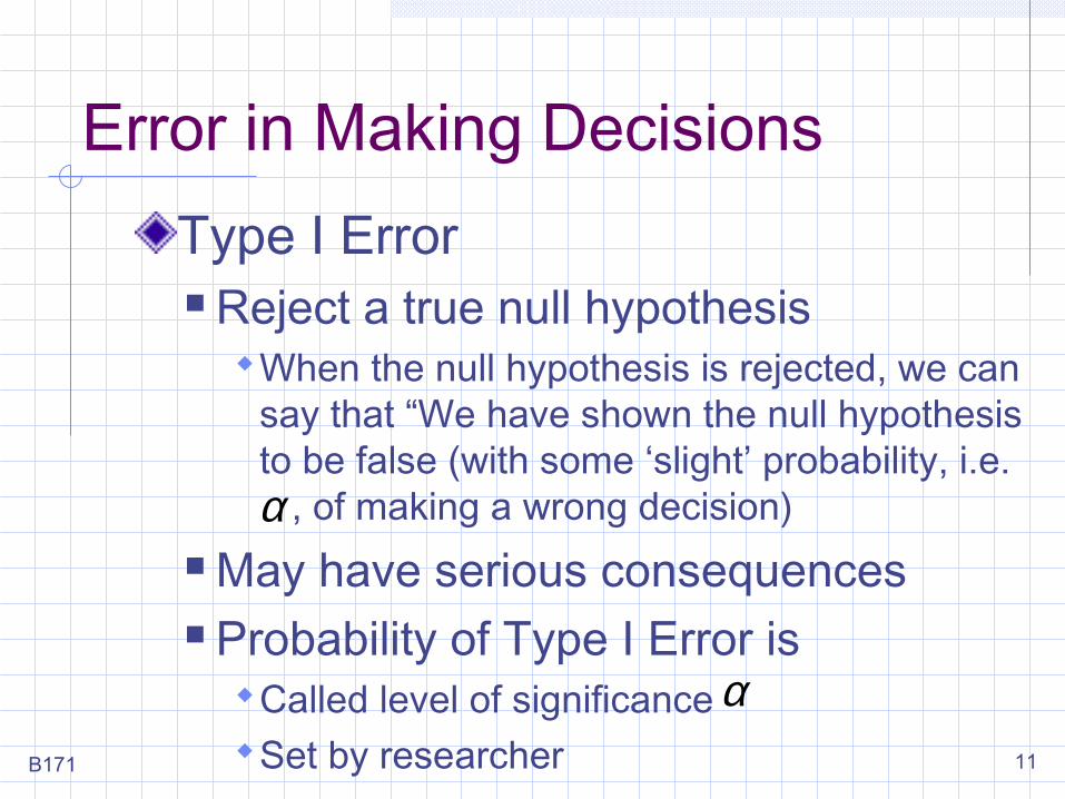
Error in Making DecisionsType I Error Reject a true null hypothesis

When the null hypothesis is rejected, we can say that “We have shown the null hypothesis to be false (with some ‘slight’ probability, i.e. , of making a wrong decision)

May have serious consequences Probability of Type I Error is

Called level of significanceSet by researcher

α

α

B171 12

Error in Making Decisions

Type II Error Fail to reject a false null hypothesis Probability of Type II Error is The power of the test is Probability of Not Making Type I Error Called the Confidence Level

( )1 α−

(continued)

( )1 β−β

B171 13

Type I and Type II ErrorActual

DecisionStatisticalDecision

H0 is true H0 is false

Reject H0

Type I error

(α)/Level of

Signif icance

Right decision

(1-β)/Power of

Test

Do not reject H0

Right decision

(1-α)/Level of

ConfidenceType II error (β)

B171

Example

14

Mr. Chan is the QC manager on a production line. He has to monitor the output to ensure that the proportion of defective products is less than 0.5%. Hence, he periodically selects a random sample of the items produced to perform a hypothesis test accordingly.

1)State the corresponding H0 and H1 for the above scenario. 2)For the given situation, what is a type I error and what is a type II error? Explain briefly. 3)Which type of error might Mr. Chan considers more serious? Explain briefly.

B171

Solutions1)H0 : The proportion of defective quality products is not less than 0.5%.H1 : The proportion of defective products is less than 0.5%.

2)A type I error means that the actual proportion of defective products is not less than 0.5% but it was considered to be less than 0.5%.A type II error means that the actual proportion of defective products is less than 0.5% but it was considered to be not less than 0.5%.

3)Mr. Chan might consider a type I error be more serious since its consequence implies that his customer has a higher chance of buying a low-quality product because Mr. Chan wrongly believes that the quality of the output is up to the required standard when in fact it is not. 15

B171 16

Hypothesis Testing Process

Identify the Population

Assume thepopulation

mean GPA is 3.5

( )

REJECT

Take a Sample

Null Hypothesis

No, not likely!

X 2.4 likely if Is 3.5?µ= =

0 : 3.5H µ =

( )2.4X =

( )5.3:1 ≠µH

11

22

3344

B171 17

= 3.5

It is unlikely that we would get a sample mean of this value ...

... if in fact this were the population mean.

... Therefore, we reject the

null hypothesis that = 3.5.

Reason for Rejecting H0

µ

Sampling Distribution of

2.4

If H0 is trueX

X

µ11

22 33

B171 18

Accept or reject the hypothesis?

See whether test statistic falls into acceptance region or rejection regionDue to the uncertainty associated with making a Type II error, we often recommended that we use the statement

“Do not reject H0” instead of “Accept H0”

Please take note that:

When we reject H0, it does not mean that we have proved it to be false.

Since we are not proving that H0 is true and we do not certain about the

probability of making Type II error, it is wiser to say ‘do not reject H0’

instead of ‘accept H0’

B171 19

Level of Significance, Defines Unlikely Values of Sample Statistic if Null Hypothesis is True Called rejection region of the sampling

distributionDesignated by , (level of significance) Typical values are .01, .05, .10

Selected by the Researcher at the BeginningControls the Probability of Committing a Type I ErrorProvides the Critical Value(s) of the Test

α

α

B171 20

Level of Significance and the Rejection Region

H0: µ ≥ 3.5

H1: µ < 3.50

0

0

H0: µ ≤ 3.5

H1: µ > 3.5

H0: µ = 3.5

H1: µ ≠

3.5

α

α

α /2

Critical Value(s)

Rejection Regions

B171 21

Inference about a population mean with a known population standard deviation (p.15 of Study Unit 4)

Two approaches:The rejection (critical) region

approachp-value approach

B171 22

Rejection Region Approach to Testing

Convert Sample Statistic (e.g., ) to Test Statistic (e.g., Z, t or F –statistic)Obtain Critical Value(s) for a Specifiedfrom a Table or Computer If the test statistic falls in the critical (or

rejection) region, reject H0

Otherwise, do not reject H0

X

α

B171 23

The rejection region is a range of values such that if the test statistic falls into that range, the null hypothesis is rejected in favor of the alternative hypothesis.

The rejection region is a range of values such that if the test statistic falls into that range, the null hypothesis is rejected in favor of the alternative hypothesis.

Define the value of that is just large enough to reject the null hypothesis as . The rejection region is

xLx

Lxx ≥

The Rejection Region Approach

is the critical value.LX

B171 24

Do not reject the null hypothesis

Reject the null hypothesis

Lxx ≥The Rejection region is:(for one-tailed test)

Lxx >LxLxx <

Acceptance RegionCritical Value Rejection Region

B171 25

Finding critical value

Determine the αFor a given σ and n, the critical value is

If , reject H0; otherwise do not reject H0

µσσ

µ

α

α

+=⇒

=−

n

zx

zn

x

L

L

Lx

Lxx >

B171 26

Instead of using the statistic , we can use the standardized value z.

Then, the rejection region becomes

x

n

xz

σµ−=

αzz ≥One-tail test

The standardized test statistic

B171 27

General Steps in Hypothesis Testing

E.g., Test the Assumption (Claim) that the True Mean # of TV Sets in U.S. Homes is at Least 3 ( Known)σ

1. State the H0

2. State the H1

3. Choose

4. Choose n5. Choose Test

0

1

: 3

: 3

=.05

100

Z

H

H

n

test

µµ

α

≥<

=α

B171 28

100 households surveyedComputed test stat =-2,

p-value = .0228Reject null hypothesisThere is evidence that the true

mean # TV set is less than 3 at 0.05 level of significance

(continued)

Reject H0

α

-1.645Z

6. Set up critical value(s)

7. Collect data

8. Compute test statistic and p-value

9. Make statistical decision

10.Draw conclusion

General Steps in Hypothesis Testing

B171 29

p-Value Approach to Testing (p.20-p.26 of Study Unit 4)

Convert Sample Statistic (e.g., ) to Test Statistic (e.g., Z, t or F –statistic)Obtain the p-value from a table or computer p-value: probability of obtaining a test statistic as

extreme or more extreme ( or ) than the observed sample value given H0 is true

Called observed level of significance Smallest value of that an H0 can be rejected

Compare the p-value with for one-tailed test If p-value , do not reject H0

If p-value , reject H0

X

≤ ≥

<≥ α

α

αα

Steps:

B171 30

The p - value provides information about the amount of statistical evidence that supports the alternative hypothesis.

– The p-value of a test is the probability of observing a test statistic at least as extreme as the one computed, given that the null hypothesis is true.

P-Value Approach

Use commonly in computer software Change the Step 8 (Slide 28) as Find the p-

value

B171 31

Describing the p-value If the p-value is less than 1%, there is

overwhelming evidence that support the alternative hypothesis.

If the p-value is between 1% and 5%, there is a strong evidence that supports the alternative hypothesis.If the p-value is between 5% and 10% there is a weak evidence that supports the alternative hypothesis.If the p-value exceeds 10%, there is no evidence that supports of the alternative hypothesis.

B171 32

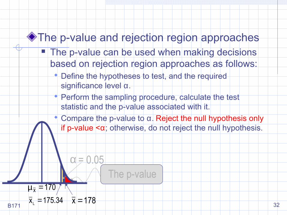
The p-value and rejection region approaches The p-value can be used when making decisions

based on rejection region approaches as follows: Define the hypotheses to test, and the required

significance level α. Perform the sampling procedure, calculate the test

statistic and the p-value associated with it. Compare the p-value to α. Reject the null hypothesis only

if p-value <α; otherwise, do not reject the null hypothesis.

The p-value

34.175xL =

α = 0.05

170x =µ178x =

B171 33

If we reject the null hypothesis, we conclude that there is enough evidence to infer that the alternative hypothesis is true.

If we do not reject the null hypothesis, we conclude that there is not enough statistical evidence to infer that the alternative hypothesis is true.

If we reject the null hypothesis, we conclude that there is enough evidence to infer that the alternative hypothesis is true.

If we do not reject the null hypothesis, we conclude that there is not enough statistical evidence to infer that the alternative hypothesis is true. The alternative hypothesis

is the more importantone. It represents whatwe are investigating.

The alternative hypothesisis the more importantone. It represents whatwe are investigating.

Conclusions of a test of Hypothesis

B171 34

One-Tail Z Test for Mean( Known)Assumptions Population is normally distributed If not normal, requires large samples (i.e.

n≥30) Null hypothesis has or sign only is knownZ Test Statistic

σ

≤ ≥

/X

X

X XZ

n

µ µσ σ− −= =

σ

B171 35

Rejection Region

Z0

Reject H0

Z0

Reject H0

H0: µ ≥ µ0 H1: µ < µ0

H0: µ ≤ µ0 H1: µ > µ0

Z must be significantly below 0 to reject H0

Small values of Z don’t contradict H0 ; don’t reject

H0 !

αα

B171 36

Example: One-Tail Test

Does an average box of cereal contain more than 368 grams of cereal? A random sample of 25 boxes showed = 372.5. The company has specified σ to be 15 grams. Test at the α = 0.05 level.

368 gm.

H0: µ ≤ 368 H1: µ > 368

X

B171 37

Reject and Do Not Reject Regions

Z0 1.645

.05

Reject

1.50

X368XXµ µ= = 372.5

0 : 368H µ ≤

1 : 368H µ >

Do Not Reject

B171 38

Finding Critical Value: One-Tail

Z .04 .06

1.6 .4495 .4505 .4515

1.7 .4591 .4599 .4608

1.8 .4671 .4678 .4686

.4738 .4750

Z0 1.645

.05

1.9 .4744

Standardized Cumulative Normal Distribution Table

(Portion)What is Z given α = 0.05?

α = .05

Critical Value = 1.645

.5+.45 = .95

1Zσ =

B171 39

Example Solution: One-Tail Test

α = 0.05

n = 25

Critical Value: 1.645

Decision:

Conclusion:

Do Not Reject H0 at a = .05, since Z=1.5<1.645

There is Insufficient Evidence that True Mean is More Than 368 at 0.05 level of significance.

Z0 1.645

.05

Reject

H0: µ ≤ 368 H1: µ > 368

1.50X

Z

n

µσ

−= =

1.50

B171 40

p -Value Solution

Z0 1.50

p-Value =.0668

Z Value of Sample Statistic

From Z Table: Lookup 1.50 to Obtain .4332

Use the alternative hypothesis to find the direction of the rejection region.

0.5000 - .4332 .0668

p-Value is P(Z ≥ 1.50) = 0.0668

3

1

2

B171 41

p -Value Solution (continued)

01.50

Z

Reject

(p-Value = 0.0668) > (α = 0.05) Do Not Reject.

p Value = 0.0668

α = 0.05

Test Statist ic 1.50 is in the Do Not Reject Region

1.645

4

B171 42

Example: Two-Tail TestDoes an average box of cereal contain 368 grams of cereal? A random sample of 25 boxes showed = 372.5. The company has specified σ to be 15 grams and the distribution to be normal. Test at the α = 0.05 level.

368 gm.

H0: µ = 368

H1: µ ≠ 368

X

B171 43

Reject and Do Not Reject Regions

Z0 1.96

.025

Reject

-1.96

.025

1.50

X368XXµ µ= = 372.5

Reject

0 : 368H µ =

1 : 368H µ ≠

B171 44

372.5 3681.50

1525

XZ

n

µσ

− −= = =α = 0.05

n = 25

Critical Value: ±1.96

Example Solution: Two-Tail Test

Test Statistic:

Decision:

Conclusion:

Do Not Reject H0 at α = .05 since -1.96 < (Z=1.5) < 1.96

Z0 1.96

.025

Reject

-1.96

.025

H0: µ = 368

H1: µ ≠ 368

1.50

There is insufficient evidence that true mean is not 368 at 0.05 level of significance.

Since σ is known, we use Z-test

B171 45

p-Value Solution


01.50

Z

Reject

α = 0.05

1.96

p-Value = 2 x 0.0668

(for two-tailed test)


Reject

B171 46

Interval estimators can be used to test hypotheses.

Calculate the 1 - α confidence level interval estimator, then if the hypothesized parameter value falls within

the interval, do not reject the null hypothesis, while

if the hypothesized parameter value falls outside the interval, conclude that the null hypothesis can be rejected (µ is not equal to the hypothesized value).

Testing hypotheses and intervals estimators

B171 47

( ) ( )

For 372.5, 15 and 25,

the 95% confidence interval is:

372.5 1.96 15 / 25 372.5 1.96 15 / 25

or

366.62 378.38

X nσ

µ

µ

= = =

− ≤ ≤ +

≤ ≤

Connection to Confidence Intervals

We are 95% confident that the population mean is

between 366.62 and 378.38.

If this interval contains the hypothesized mean (368),

we do not reject the null hypothesis.

It does. Do not reject.

H0: µ = 368

H1: µ ≠ 368

H0 at 0.05 level of significance

nZX

δα

2±

B171 48

Drawbacks Two-tail interval estimators may not provide the

right answer to the question posed in one-tail hypothesis tests.

The interval estimator does not yield a p-value.

There are cases where only tests (rejection region approach or p-value approach) producethe information needed to make decisions.

B171 49

Inference About a Population Mean with Unknown Standard Deviation

For unknown σ, with small samples (n<30), t-test is used.Test statistic

with d.f. (n-1)ns

xtn

µ−=−1

B171 50

Checking the required conditions/assumptions for using t-distribution

We need to check that the population is normally distributed, or at least not extremely non-normal. We can plot the histogram of the data set to verify its normality.

B171 51

Example: One-Tailed t Test

Does an average box of cereal contain more than 368 grams of cereal? A random sample of 36 boxes showed X = 372.5, and s = 15. Test at the α = 0.01 level.

368 gm.

H0: µ ≤ 368 H1: µ > 368

σ is not given

B171 52

Example Solution: One-Tailed

α = 0.01

n = 36, df = 35


Test Statistic:

Decision:

Conclusion:

Do Not Reject H0 at = .01 since t=1.80<2.4377

t350 2.4377

.01

Reject

H0: µ ≤ 368 H1: µ > 368

372.5 3681.80

1536

Xt

Sn

µ− −= = =

1.80

There is Insufficient Evidence that True Mean is More Than 368 at 0.01 level of significance.

α

Please take note that you may use Z-test in this case since n>30. But t-test is an exact method in this case. Therefore, both tests are acceptable in this case.

B171 53

p -Value Solution

01.80

t35

Reject

t = 1.8 & d.f. = 35

(p-Value is between .025 and .05) > (α = 0.01) Do Not Reject.

p-Value = [.025, .05]

α = 0.01


2.4377

B171 54

Example: Two-Tailed t Test

Does an average box of cereal contain 368 grams of cereal? A random sample of 36 boxes showed X = 372.5, and s = 15. Test at the α = 0.01 level.

368 gm.

H0: µ = 368 H1: µ ≠ 368 σ is not given

B171 55

Example Solution: Two-Tailed

α = 0.01

n = 36, df = 35


Test Statistic:

Decision:

Conclusion:

Do Not Reject H0 at = .01 since -2.724< t=1.80 <2.724

t350 2.724

.005

Reject

H0: µ = 368 H1: µ ≠ 368

372.5 3681.80

1536

Xt

Sn

µ− −= = =

1.80

There is Insufficient Evidence that True Mean is 368 at 0.01 level of significance.

α

Please take note that you may use Z-test in this case since n>30. But t-test is an exact method in this case. Therefore, both tests are acceptable in this case.

0.005

-2.724

Reject

B171 56

p -Value Solution

01.80

t35

Reject

t = 1.8 & d.f. = 35p-Value is between 2x(.025 and .05) > (α = 0.01) i.e. p-Value is between (.05 and .1) > (α = 0.01)

Do Not Reject H0.

(p-Value)/2 = [.025, .05]

α /2= 0.005

Test Statist ic 1.80 is in the ‘Do Not Reject H 0‘ Region

2.724

Reject

α /2= 0.005

2.724

B171 57

Connection to Confidence IntervalsH0: µ = 368

H1: µ ≠ 368

α= 0.01n=36, df = 35

For and n =25, the 99% confidence interval is:

372.5 – (2.797) ≤ µ ≤ 372.5 + (2.797) or364.11 ≤ µ ≤ 380.89

15,5.372 == SX

n

StX

2α±

We are 99% confident that the population mean is between 364.11 and 380.89. Since this interval contains the hypothesized mean (368), we do not reject H0 at 0.01 level of significance.

B171 58

Inference About a Population Proportion

Use in qualitative or categorical dataOnly inference about the proportion of occurrence of a certain valueTest statistic

provided that is approx. normal and both np and n(1-p) are greater than 5

npp

ppz

/)1(

ˆ

−−=

p̂

B171 59

ProportionSample Proportion in the Success Category is Denoted by pS

When Both np and n(1-p) are at Least 5, pS Can Be Approximated by a Normal Distribution with Mean and Standard Deviation

(continued)

Number of Successes

Sample Sizes

Xp

n= =

sppµ = (1 )

sp

p p

nσ −=

B171 60

Example: Z Test for Proportion

( )

( ) ( )

Check:

500 .04 20

5

1 500 1 .04

480 5

np

n p

= =≥− = −

= ≥

A marketing company claims that a survey will have a 4% response rate. To test this claim, a random sample of 500 were surveyed with 25 responses. Test at the α = .05 significance level.

B171 61

0.05

Critical Values: ± 1.96

1.1411

( ) ( ).05 .04

1.14111 .04 1 .04

500

Sp pZ

p p

n

− −≅ = =− −

Z Test for Proportion: Solution

α = 0.05

n = 500

Do not reject H0 at α = .05 since

-1.96 < (Z=1.1411) < 1.96

H0: p = 0.04

H1: p ≠

0.04

Test Statistic:

Decision:Conclusion:

Z0

Reject Reject

.025.025

1.96-1.96

We do not have sufficient evidence to reject the company’s claim of 4% response rate at 0.05 level of significance.

SP0.04

Two-tailed Test

B171 62

p -Value Solution


01.1411

Z

Reject

α = 0.05

1.96

p-Value = 2 x .1271

(for two-tailed test)


Reject

B171 63

0.05

Critical Values: 1.645

1.1411

( ) ( ).05 .04

1.14111 .04 1 .04

500

Sp pZ

p p

n

− −≅ = =− −

Z Test for Proportion: Solution

α =0.05

n = 500

Do not reject H0 at α = .05 since

Z=1.1411 < 1.645

H0: p ≤0 .04

H1: p >

0.04

Test Statistic:

Decision:Conclusion:

Z0

Reject

0.05

1.645

We do not have sufficient evidence to reject the company’s claim of at most 4% response rate at 0.05 level of significance.

SP0.04

One-tailed Test

B171 64

p -Value Solution

(p-Value = 0.1271) > (α = 0.05) Do Not Reject H0.

01.1411

Z

Reject

α = 0.05

1.645

p-Value = 0.5 – 0.3729 =0.1271


B171 65

Connection to Confidence IntervalsH0: p = 0.04

H1: p ≠ 0.04

α= 0.05n=500

For ps = 0.05, the 95% confidence interval is:

i.e. 0.0309 ≤ p ≤ 0.0691 We are 95% confident that the population proportion

is between 0.0309 and 0.0691. Since this interval contains the hypothesized proportion of 0.04, we do not reject H0 at 0.05 level of significance.

( ) ( )500

05.0105.096.105.0

12

−±=−

±n

PPZP SS

S α

B171 66

Inference About a Population Variance

Some times we are interested in making inference about the variability of processes.Examples: The consistency of a production process for

quality control purposes. Investors use variance as a measure of risk.

To draw inference about variability, the parameter of interest is σ2.

B171 67

The sample variance s2 is an unbiased, consistent and efficient point estimator for σ2.The statistic has a distribution called Chi-squared, if the population is normally distributed.

2

2s)1n(

σ−

1n.f.ds)1n(

2

22 −=

σ−=χd.f. = 1

d.f. = 5 d.f. = 10

The test statistic used to draw conclusions about the variability is called a “Chi-squared test statistics’

1,122

−−= nαχχCritical Value of

B171 68

A

A

χ2Αχ2

1-A

The χ2 table (p.52 of Study Unit 4)

Degrees offreedom

1 0.0000393 0.0001571 0.0009821 . . 6.6349 7.87944..

10 2.15585 2.55821 3.24697 . . 23.2093 25.1882. . . . . .. . . . . . . .

χ2.995 χ2

.990 χ2.975 χ2

.010 χ2.005

.990 .010

=.01

=.01

1 - A =.99A

χ2.01,10 = 23.2093

Chi-squared Distr ibution

**Please take note that it may not be possible to find out an exact p-value from the Chi-squared table. To find a p-value, we can use Excel (Refer to p.42 of Study Unit 4).

B171 69

B171 70

B171 71

Estimating the population variance

(1-α)100% Confidence Interval:From the following probability statement

P(χ21-α/2 < χ2 < χ2

α/2) = 1-αwe have (by substituting

χ2 = [(n - 1)s2]/σ2.)

21,2/1

22

21,2/

2 )1()1(

−−−

−<<−

nn

snsn

αα χσ

χ

B171 72

χ2 test statistic and decision rule (Please also refer to Example 4.5 on pp.41 of Study Unit 4)

Similar to mean and proportionTest statistic

Decision rule: Reject H0 if Two-tailed: Right-tailed: Left-tailed:

20

22 )1(

σχ sn −=

21

22

22

22)21(

2 or

α

α

αα

χχχχ

χχχχ

−

−

<

>

><

B171 73

Example Consider a container f i l l ing machine. Management wants a machine to f i l l 1 l i ter (1,000 cc ’s) so that that variance of the f i l ls is less than 1 cc 2. A random sample of n=25 1 l i ter f i l ls were taken. Does the machine perform as it should at the 5% signif icance level?

IDENTIFY

1000.31001.3999.5999.7999.3

999.8998.31000.

6999.7999.8

1001999.4999.5998.5

1000.7

999.6999.81000998.2

1000.1

998.11000.7999.8

1001.31000.7

Data

B171 74

Example

Variance is less than 1 cc 2

(n – 1)s2

χ2 = σ2

We want to show that: H1: σ2 < 1

(so our null hypothesis becomes: H0: σ2 = 1). We will use this test statistic:

IDENTIFY

B171 75

ExampleSince our alternative hypothesis is phrased as:

H 0: σ2 = 1 H 1: σ2 < 1We wil l reject H 0 in favor of H 1 i f our test statistic falls into this rejection region:

We computer the sample variance to be: s 2=0.8088And thus our test statistic takes on this value…

COMPUTE

compare

χ2 < χ2 = χ21-.05, 25-1 = χ2

.95,24= 13.8484 1-α,n-1

(n – 1)s2

χ2 = σ2

(25 – 1)(0.8088) = = 19.41

1

B171 76

13.8484 19.41

Rejectionregion

8484.132 <χ2χ

2125,95. −χ

α = .05 1-α = .95

Do not reject the null hypothesis

ExampleSince:

There is not enough evidence to infer that the claim is true

at 0.05 level of significance.

INTERPRET

B171 77

ExampleAs we saw, we cannot reject the null hypothesis in favor of the alternative. That is, there is not enough evidence to infer that the claim is true.Note: the result does not say that the variance is greater than 1, rather it merely states that we are unable to show that the variance is less than 1.

We could estimate (at 99% confidence say) the variance of the fi l ls…

B171 78

Example In order to create a confidence interval estimate of the variance, we need these formulae:

we know (n–1)s 2 = 19.41 from our previous calculat ion, and we have from Table 5 in Appendix B:

COMPUTE

lower confidence l imit upper confidence l imit

χ2α/2,n-1 = χ2

.005,24 = 45.5585

χ21−α/2,n-1 = χ2

.995,24 =9.88623

B171 79

ExampleThus the 99% confidence interval estimate is:

That is, the variance of f i l ls l ies between .426 and 1.963 cc 2.H 0: σ 2 = 1 H 1: σ 2 ≠ 1

We are 99% confident that the population variance is between 0.426 and 1.963. Since this interval contains the hypothesized variance of 1, we do not reject H 0 at 0.01 level of signif icance.

COMPUTE

B171 80

Thank You!

~ THE END ~

Study unit 4 (oct 2014)

Business

Transcript of Study unit 4 (oct 2014)