Study on the limitations of travel-time inversion applied to sub...

Solid Earth, 4, 543–554, 2013www.solid-earth.net/4/543/2013/doi:10.5194/se-4-543-2013© Author(s) 2013. CC Attribution 3.0 License.

Solid Earth

Open A

ccess

Study on the limitations of travel-time inversion applied tosub-basalt imaging

I. Flecha1, R. Carbonell1, and R. W. Hobbs2

1Departament de Estructura i Dinàmica de la Terra, Institut de Ciències de la Terra Jaume Almera-ICTJA-CSIC,C/ Lluís Solé i Sabarís s/n, 08028, Barcelona, Spain2Department of Earth Sciences, University of Durham, Durham DH1 3LE, UK

Correspondence to:R. Carbonell ([email protected])

Received: 12 February 2013 – Published in Solid Earth Discuss.: 20 March 2013Revised: 3 November 2013 – Accepted: 5 November 2013 – Published: 23 December 2013

Abstract. The difficulties of seismic imaging beneath highvelocity structures are widely recognised. In this setting, the-oretical analysis of synthetic wide-angle seismic reflectiondata indicates that velocity models are not well constrained.A two-dimensional velocity model was built to simulate asimplified structural geometry given by a basaltic wedgeplaced within a sedimentary sequence. This model repro-duces the geological setting in areas of special interest for theoil industry as the Faroe-Shetland Basin. A wide-angle syn-thetic dataset was calculated on this model using an elasticfinite difference scheme. This dataset provided travel timesfor tomographic inversions. Results show that the originalmodel can not be completely resolved without consideringadditional information. The resolution of nonlinear inver-sions lacks a functional mathematical relationship, therefore,statistical approaches are required. Stochastic tests based onMetropolis techniques support the need of additional infor-mation to properly resolve sub-basalt structures.

1 Introduction

Sub-salt and sub-basalt imaging has been a key objective dur-ing the last 2 decades for the oil exploration (Rousseau et al.,2003; Williamson, 2003; Sava and Biondi, 2004). Oil explo-ration has revealed the imaging difficulties in the presenceof high velocity features (such as salt and/or basalts). Lowvelocity structures under relatively high velocity featuresare poorly constrained by conventional processing and/orinversion schemes (Flecha et al., 2004). Velocity providesthe link between seismic images and rock types. Ray trac-

ing theory, based on Fermat’s principle, states that regionssurrounded by higher velocities are under-sampled by rays.Seismic images of the subsurface strongly benefit from wellresolved estimation of seismic velocities. These seismic ve-locities are currently determined by velocity analysis and,in the best case, by travel time tomography (or by the in-version of travel time of first arrivals) of wide-angle seis-mic reflection/refraction shot-gathers (Zelt and Smith, 1992).The determination of the velocity models requires the inter-pretation/identification of the seismic arrivals within a shot-gather. Furthermore, the mathematical inversion schemes re-quire digitized travel times, offset pairs, to calculate veloci-ties. Usually, a standard crustal velocity model features an in-creasing velocity with depth, however in the presence of saltand/or basaltic intrusions this assumption fails. Intrusions of-ten represent the emplacement of a high velocity body in thecrust, therefore zones beneath these structures may featurelow velocities. This is the case of basalt covered areas aserupted basalt buries previous structures that may feature lowvelocities such as in the Faroe Shelf. In the Faroe Shelf, cov-ered areas represent potential hydrocarbon reservoirs, there-fore this topic is of special interest for the industry.

This manuscript develops a theoretical study investigat-ing the reliability and effectiveness of travel time inversionof wide-angle seismic reflection/refraction data. We inves-tigated when and to what extent the low velocity structurebeneath a high velocity basalt layer can be resolved by usingtravel times alone. This manuscript is not aimed to present anspecific inversion scheme, the validity and calibration of theinversion scheme used here is presented elsewhere (Trinkset al., 2005). Also relatively recent new developments which

Published by Copernicus Publications on behalf of the European Geosciences Union.

544 I. Flecha et al.: Study on the limitations of travel-time inversion applied to sub-basalt imaging

are more computationally expensive such as full waveforminversion could be employed to constraint sub-basalt fea-tures, however, these approaches are beyond the scope of thiscontribution.

2 Geological setting and imaging problems

In the Faroe-Shetland Basin, Mesozoic and Tertiary sedimen-tary sequences fill the basin but, close to the Faroe Shelf,these sedimentary sequences are covered by Paleocene-Eocene basaltic lavas of which the Faroe Islands are com-posed. The previous topography of the basin was dominatedby normal faults as a consequence of the extension and sub-sidence during Cretaceous and Paleocene (Richardson et al.,1999). As huge amounts of molten rock were extruded, af-ter filling the lows between fault blocks, lava flows extendedover long distances in the basin. Basalt flows were eruptedin several episodes and three major units have been identi-fied: Lower, Middle and Upper Series. The composition andthickness differs from one unit to another. Moreover, in peri-ods without igneous activity, lacustrine shales and coals wereaccumulated and sediments were emplaced filling the basinfloor deeps (White et al., 2003).The resulting structure in theFaroe-Shetland Basin may be considered as a relatively thinwedge/finger of basaltic rocks emplaced within a sedimen-tary sequence This structure developed within the tectonicframework of the evolution of the North Atlantic IgneousProvince and the opening of the NE Atlantic rift (Jolley andBell, 2002).

In the Faroe Shelf, geologic and geophysical data suggestthat a layer of basalt is placed within two low velocity sedi-mentary sequences (Hughes et al., 1998; Richardson et al.,1998, 1999; Fliedner and White, 2003; Smallwood et al.,2001; Sørensen, 2003; White et al., 2003; Raum et al., 2005).The velocity structure for sediments above the basalt can beresolved by conventional techniques. The top of the basaltlayer can be determined very effectively due to the high con-trast in seismic physical properties between the basalt and theoverlying sediments. However, the high velocity basalt layerrepresents a complex scenario for seismic imaging method-ologies, acting as a barrier so that the underlying structurescan not be imaged. The high velocity that characterises thebasalt contrasts with relatively low velocity of the surround-ing materials. This causes that most of energy is reflectedand/or travels along this layer. Furthermore, the heteroge-neous structure of the basalt layers scatter 100 the higherseismic frequencies of the source signal (Pujol and Smithson,1991; Hobbs, 2002). The lack of penetration and the multiplescattering within the basalt layer obscures the potential seis-mic events generated bellow the basalt. This could representpotentially prospective sedimentary structures.

Although basalt flows tend to be sub-horizontal on largescale, at small scale, rugged interfaces cause scattering anddisperse the elastic energy destroying any lateral coherency

of possible sub-basalt events. In addition to the differencesbetween the three major Series, within every unit, basalticbodies are highly heterogeneous in composition and phys-ical properties. These heterogeneities strongly disperse theseismic energy and destroy the signal coherence in the seis-mic wave-field (Pujol and Smithson, 1991). The outer partsof the basalt flows are affected by weathering causing a de-crease in velocity, this contrasts with the internal parts whichcooled slowly and without any external influence preservinga high velocity feature. Interfaces between individual flowsin a basalt block produce internal multiples and wave con-versions. Also some intrusive basalt flows were emplaced assills within previous structures providing an additional causefor scattering at and beneath the base of the basalt.

In addition to these major imaging issues, the usual prob-lems of marine seismic reflection data acquisition must bealso considered (tidal noise, multiples, peg-leg, reverbera-tion, converted-waves, etc.). In the Faroe Shelf, conventionalseismic reflection techniques are insufficient to study sub-basalt structures. Sub-basalt imaging is very sensitive to ac-quisition and processing parameters. In acquisition, long off-set 2-D and 3-D seismic data can contribute to an improve-ment in the seismic image below top basalt. Increasing thesource energy at low frequencies by: towing the source andreceiver cables at deeper levels and/or using bubble-tunedrather than conventional peak-tuned source arrays. Furtherimprovement can be provided by High frequencies (domi-nantly noise) are filtered out of the data early in the process-ing to concentrate on the low frequency data. Careful multi-ple removal is important with several passes of de-multiplebeing applied to the data using both Surface-Related Mul-tiple Elimination (SRME) and Radon techniques. Velocityanalysis is performed as an iterative process taking into ac-count the geological model. In summary sub-basalt imaginghas undergone remarkable advances in last years, these im-provements consist in designing new geometry acquisitionpatterns (White et al., 2003), designing new sources (Stapleset al., 1999; White et al., 2002; Ziolkowski et al., 2003), un-derstanding the scattering caused by the basalt (Martini et al.,2001; Martini and Bean, 2002) or combining several geo-physical methodologies (Jegen-Kulcsar and Hobbs, 2005).Nevertheless, studying sub-basalt structures requires a de-tailed velocity model to obtain valuable information and toapply more sophisticated approaches such as prestack depthmigration.

3 Theoretical geologic model and synthetic seismic data

A synthetic dataset was acquired using an idealised veloc-ity model. The model consists of a wedge of basalt layerwithin a sedimentary column. The basalt layer features anirregular upper surface, and very high velocities and densi-ties that contrast with the velocities and densities of the sur-rounding sediments. The choice of a thin wedge for the basalt

Solid Earth, 4, 543–554, 2013 www.solid-earth.net/4/543/2013/

I. Flecha et al.: Study on the limitations of travel-time inversion applied to sub-basalt imaging 545

Table 1.Velocities and densities used in the synthetic model. Phys-ical properties were taken fromCarmichael(1982). The Poissonratio was 0.25 and the density was calculated using the ChristensenrelationChristensen and Mooney(1995): ρ = 1.85+ 0.169Vp.

Layer Vp Vs ρ

Water 1.5 0.86 1.00Sediment1 2.1 1.21 2.20Sediment2 2.3 1.33 2.24Sediment3 2.6 1.50 2.29Basalt 5.3 3.06 2.75Sediment4 3.0 1.73 2.36Sediment5 3.5 2.02 2.44Sediment6 3.9 2.25 2.51Basement 6.0 3.46 2.86

is justified because it represents the best geological settingfor exploration and exploitation for the oil industry. In or-der to simulate a highly variable structure, we consider thesmall-scale top basalt topography to be a random field whichwas generated using Von Karman functions (Goff and Jor-dan, 1988). As there is a high velocity contrast between thesedimentary cover and the basalt, can this topography be re-covered? In addition, in the case of Shetland-Faroe Basin, thearea where the basalt thins is close to the center of the basinwhere geology is well known and can be extrapolated to sug-gest the existence of sub-basalt sedimentary structures. TheP-wave velocities were taken from laboratory measurements(Carmichael, 1982). All the physical properties used in thesimulation are summarised in Table1.

A second order finite difference solver of the elastic waveequation using Sochacki’s interface scheme (Sochacki et al.,1987, 1991) was used to generate a seismic dataset acquiredover the velocity model. The 2-D model was of 100 km wideand 8 km deep and a 10× 10 m grid was used (Fig.1). Af-ter intense calculations, 80 shot-gathers were simulated withmore than 3000 traces per shot (one trace every 30 m) and30 s of recording time. The sampling for this synthetic datasetwas 1 ms. The parameters for these simulations are sum-marised in Table2. In this data several phases were identified(Fig. 2). The source wavelet is a minimum phase waveletwith a frequency content of 5 to 25 Hz. Travel time datawas picked using the peak amplitude as the reference andan estimated uncertainty of 0.010 s was used in the inversionscheme.

Water multiple and peg-leg signal were generated by theelastic finite difference algorithm, no additional noise wasincluded in the data. Although in nature, basalts appear ashighly heterogeneous layered structures, in order to simplifythe problem, the basaltic wedge was considered as an ho-mogeneous feature in its internal velocity distribution. Underthese conditions we obtained a quite ideal dataset.

Table 2.Parameters used to generate synthetic data.

Synthetic data parameters

Model length 100 kmModel depth 8 kmCell size 10× 10 mNumber of shots 80Number of channels 3294Station spacing 30 mRecording length 30 sSource spacing 1 kmSample rate 1 ms

Fig. 1. Synthetic velocity model resampled using 100× 100 msquared cells. The original model used to run simulations was sam-pled by 10× 10 squared cells. Vertical lines at 10 and 50 km showthe location of hypothetical wells drilled through the basalt layer.Thus at this points, the thickness of the basaltic wedge was known.This information was used in the inversion (see text for more expla-nation).

4 Tomographic inversions

The main aim of synthetic simulations was checking the pos-sibility of recovering the original model using tomographictechniques. As a first attempt, first arrivals travel time seis-mic tomography was applied using the TTT software pack-age (Trinks et al., 2005). This code is based on initial valueray tracing in velocity models constructed of Delaunay trian-gulated grids and interfaces. The tomography is implementedas a joint interface and velocity inversion using the bi-conjugated gradient method. The TTT algorithm presented inTrinks(2003) andTrinks et al.(2005) is based on the methodby McCaughey and Singh(1997); Hobro et al.(2003) withthe advantage that allows for irregular parametrized-velocitygrids using Delaunay triangulation. The velocities are de-fined at triangle vertices, then a linear interpolation is used tocalculate the slowness squared within the triangle. Note thatthe velocity field is defined by the slowness squared (slothmodels (Muir and Dellinger, 1985) this parametrization re-sults in fast calculation of the analytic solution to the raytracing equations. This approach avoids the discontinuities

www.solid-earth.net/4/543/2013/ Solid Earth, 4, 543–554, 2013


Fig. 2.Synthetic shotgather. Different phases can be identified: wa-ter wave (blue), refraction from sediments over the basalt layer(green), refraction from basalt (red), reflection from the top of thebasalt (yellow), refractions from basement (purple) and reflectionsfrom the top of the basement (orange).

in ray paths that would appear when using constant velocitycells (Cervený, 2001). The appendices inTrinks et al.(2005)go to further detail in mathematics used to fill in the veloc-ity grid. Depending on the ray density the algorithm allowsfor a denser model parametrization of the densely sampledregions, increasing the resolution and efficiency of the algo-rithm. The inversion followsVesnaver(1994); Böhm(1996)scheme that reduces the non-uniqueness of the travel-timeinversion result by adapting the grid.

The forward problem is solved by using an analyticalray tracing in a medium with a linear gradient of slownesssquared (Farra, 1990; Cervený, 2001), an initial-value ray-tracing scheme with traveltime interpolation is used. Themodel parametrization and the ray-tracing approach used bythis algorithm allow for an efficient analytical computation ofthe Frechet derivatives of travel-time with respect to modelparameters.Trinks et al.(2005) demonstrates that the calcu-lation of the Frechet derivatives are only needed at the pointsalong the ray paths that correspond to the travel-times, notat every point of the model grid. Therefore, the inversion ap-proach is very efficient. Finally,Trinks et al.(2005) demon-strates this points using synthetic and real data tests. Furtherdetails on the TTT tomographic algorithm can be found inTrinks et al.(2005).

The final model3 by this adaptive tomographic inversionscheme was reached when it was able to reproduce the thetravel time data within the picking uncertainty andχ was ap-proaching 1. The average velocity structure of the zone overthe basalt layer was recovered as well as the top of the basaltlayer where a sharp velocity contrast is displayed. However,no low velocity can be reproduced under the basalt, towardthe right end of the model, where no basalt exists, some re-alistic information about velocities can be obtained for thedeepest part of the model. These results suggest that thereare physical limitations in constraining sub-basalt structuresby seismic travel time tomography.


Fig. 3. Velocity model obtained using TTT package Trinks et al. (2005) considering only first arrivals. Interfaces between layers are theones that were used in the theoretical model. Velocities over the basalt wedge are well constrained. A prominent velocity discontinuity canbe observed for the first 70 km between 3 and 4 km in depth which provides the location for the top of basalt layer. A 1 dimensional fivelayer-cake model was used as the starting model (water, sediments, a wedge of basalt, sediments and basement). Note that the interfacebetween the sediment and the underlying basalt was determined using only the first arrivals. No significant differences in the final modelwere observed by changing the velocity model 20% in the velocities and 15% in the layer finickinesses. The unresolved parts of the modelat both ends of the transect are determined from forward modelling, ray tracing.

Fig. 4. Velocity model obtained using TTT package Trinks et al. (2005) after inverting refractions from the sediments over the basalt andreflections from the top of the basalt layer. Dashed lines represent layers from inversion and continous lines the theoretical layer interfaces.Note the coincidence between dashed line and continous line in the top of the basalt layer.The unresolved parts of the model at both ends ofthe transect are determined from forward modelling, ray tracing.

Fig. 3. Velocity model obtained using TTT packageTrinks et al.(2005) considering only first arrivals. Interfaces between layers arethe ones that were used in the theoretical model. Velocities over thebasalt wedge are well constrained. A prominent velocity discontinu-ity can be observed for the first 70 km between 3 and 4 km in depthwhich provides the location for the top of basalt layer. A 1 dimen-sional five layer-cake model was used as the starting model (water,sediments, a wedge of basalt, sediments and basement). Note thatthe interface between the sediment and the underlying basalt wasdetermined using only the first arrivals. No significant differencesin the final model were observed by changing the velocity model20 % in the velocities and 15 % in the layer finickinesses. The unre-solved parts of the model at both ends of the transect are determinedfrom forward modelling, ray tracing.

TTT code can also invert additional phases. In order to in-clude all the information from phases identified in syntheticshots, a layer by layer striping inversion was performed. Asthe problem is a specific one the starting model was cho-sen relatively close to the expected solution to determine ifthe travel-time data alone was able to resolve the sub-basaltstructures, taking into account the high velocity contrasts be-tween the sediments and the basalt. In the seismic explorationarea, where this study is applicable, the 1 dimensional aver-age structure is relatively well constrained. Therefore, a rel-atively simple 1-D model was chosen as the starting model.This consists in a five layer cake model these 5 layers corre-spond to: a water layer, a sediment layer, a basalt layer char-acterised by high velocity, and second sedimentary sequenceand the basement. So velocities typical of this layers wereconsidered. A series of starting models characterised by amaximum variations of 20 % on the velocity values and 15 %in the thickness where tested with no significant variations inthe resolved final models. Top basalt interface was inferredfrom the model obtained using only first arrivals (Fig.3).Even though in the theoretical model some sub-layers wereincluded in sedimentary sequences, the contrast in veloc-ity between these sub-layers is quite smooth which makesit difficult to identify events from these interfaces, thereforethis minor discontinuities were not considered in the invertedmodel.

The additional information that TTT can use correspondsto the identification of travel-time branches related to the




Fig. 3. Velocity model obtained using TTT package Trinks et al. (2005) considering only first arrivals. Interfaces between layers are theones that were used in the theoretical model. Velocities over the basalt wedge are well constrained. A prominent velocity discontinuity canbe observed for the first 70 km between 3 and 4 km in depth which provides the location for the top of basalt layer. A 1 dimensional fivelayer-cake model was used as the starting model (water, sediments, a wedge of basalt, sediments and basement). Note that the interfacebetween the sediment and the underlying basalt was determined using only the first arrivals. No significant differences in the final modelwere observed by changing the velocity model 20% in the velocities and 15% in the layer finickinesses. The unresolved parts of the modelat both ends of the transect are determined from forward modelling, ray tracing.

Fig. 4. Velocity model obtained using TTT package Trinks et al. (2005) after inverting refractions from the sediments over the basalt andreflections from the top of the basalt layer. Dashed lines represent layers from inversion and continous lines the theoretical layer interfaces.Note the coincidence between dashed line and continous line in the top of the basalt layer.The unresolved parts of the model at both ends ofthe transect are determined from forward modelling, ray tracing.

Fig. 4. Velocity model obtained using TTT packageTrinks et al.(2005) after inverting refractions from the sediments over the basaltand reflections from the top of the basalt layer. Dashed lines repre-sent layers from inversion and continuous lines the theoretical layerinterfaces. Note the coincidence between dashed line and contin-uous line in the top of the basalt layer. The unresolved parts ofthe model at both ends of the transect are determined from forwardmodelling, ray tracing.

different features within the model. Therefore, a subjectiveinterpretation of the travel time branch is required, and thenthe picks corresponding to the branch are associated to a par-ticular structure.

4.1 Inverting phases over the basalt layer

Firstly, only the travel time branches interpreted to corre-spond to the sedimentary cover were included in the inver-sion. The results show a good recovery of the original model(Fig. 4). In the first part of the model (thin water layer, 0–30 km marked as (A) this phase appears as first break and theresults are similar to the first arrivals inversion (Fig.3) whilein the last part of the model (thick water layer, 70–100 kmmarked as (B) the picks used were not considered in first ar-rivals inversion, hence, the additional data provides furtherconstraints on the sedimentary cover over the basalt layer.

The TTT code can include also reflected arrivals in theinversion scheme. As reflections from the top of the basalt aredisplayed as a very high amplitude events, the travel times ofthe reflected phases can be identified and picked at normalincidence.

Considering the final model of the previous case as start-ing model, and, without modifying the velocity values forthis model, reflections from the top of the basalt layer wereinverted in order to obtain the topography for this interface.A detailed structure was achieved which reproduces in somedegree the rugged topography featured by the original model(Fig. 4).

4.2 Inverting refractions inside the basalt

In this case, the main aim is to constrain the base of thebasalt using the refracted waves inside this layer. Raypaths

Fig. 5. Results from the basalt refraction inversion. White dashedlines represent layers from inversion and continuous lines the theo-retical layer interfaces. The base of the basalt layer, which is overes-timated, should be delineated by raypaths. The black area representsthe part of the model sampled by rays.

are very sensitive to high velocity anomalies, therefore someconstraints on the base of the basalt should be gained by in-troducing these refractions. As no noise is present in this syn-thetic dataset, refraction from basalt can be followed up tofar offsets (Fig.2). The maximum offset to stop picking isarbitrary because there is no way to separate basalt refrac-tion from base basalt reflection. In a first picking stage, re-fractions from the basalt were picked as far as possible andinverted. The results do not fit the theoretical model, overes-timating the basalt thickness (Fig.5).

To simulate a more realistic situation, some arbitrary noisewas added to the data (Fig.6). As a result, the noise limitedthe maximum offset for picking which was considerably re-duced compared with the noise-free case. The inverted modelcorrelates better with the synthetic model (Fig.7) which iscloser to the real model. However, the range between 30 and75 km features again an overestimation of the basalt thick-ness. This effect is caused by the difficulty in differentiatingbasalt refractions from base basalt reflections which interfereat short offsets. In any case, in the travel time branch, thelimit between the basalt refraction (head wave) and the sub-basalt reflection is completely arbitrary (subjective, dependson the interpreter). The travel time picking of this arrival iscomplicated even farther by the existence of noise, and thus,the maximum picking offset depends critically on the qual-ity of the data. The consequence of this subjectivity is thatthe thickness of the basalt layer is proportional to the offsetpicked, and this effect is stronger where the basalt layer thins.

This contrasts with the conventional idea of using largeapertures for sub-basalt imaging. This strategy may be use-ful in zones with thick basalt layers but, in the case of thinbasalt layers, the basalt head wave and reflection from thebase of the basalt interfere (see below) and there is no benefitby using large apertures to infer basalt seismic properties.



Fig. 6. Synthetic shotgather with noise. Different phases can beidentified: water wave (blue), refraction from sediments over thebasalt layer (green), refraction from basalt (red), reflection from thetop of the basalt (yellow), refractions from basement (purple) andreflections from the top of the basement (orange). Note the differ-ence with Fig.2 in the refractions from basalt (red).

Fig. 7.Results from the basalt refraction inversion using picks fromdata with noise. White dashed lines represent layers from inversionand continuous lines the theoretical layer interfaces. The black arearepresents the part of the model sampled by rays. The base of thebasalt layer should be delineated by raypaths. The constrain on thethickness of the basalt layer is failing where the layer is thinner,probably due to overpicking refractions.

4.3 Inverting refractions and reflections from thebasement

As shown above, the basalt layer cannot be resolved properlyonly considering refractions within this layer. In the case ofa thicker basalt layer, reflection from the base of the basaltcould be differentiated from the basalt refraction which maycontribute to better constrain the base of this layer. How-ever, for thin layers there are no possibilities of deducing thebasaltic structure using refraction data. At this point, addi-tional information is required to constrain the basalt layerthickness, in a real case, this additional information couldbe provided by drilling through the basalt layer, fixing in thisway the velocity of the basalt, the thickness of the basalt layerand the velocity of the sediments beneath the basalt.

Fig. 8.Final result obtained using all the phases after fixing the baseof the basalt layer considering that two wells were drilled throughthis layer at 10 and 50 km. Dashed lines represent layers from in-version and continuous lines the theoretical layer interfaces. Intro-ducing additional information, the theoretical model is recoveredquite accurately. Energy dispersion caused by the topography of thebasalt wedge masks the reflected energy from the basement. There-fore, the recovered basement has an irregular top which is not realbut the influence of the overlying velocity heterogeneities.

We introduced additional information in the inversionscheme, we assumed that two wells were drilled located atx = 10 km andx = 50 km (Fig. 1). In the last part of themodel there is no basalt layer, hence the signal coherenceis preserved making it possible to identify and pick normalincidence reflections from the basement. Inverting this phase,a reliable estimation of the top of the basement was obtainedfor the last 25 km of the model which, jointly with the veloc-ity obtained in first arrival inversions, constrained the modelin this part. This results were extrapolated under the basaltlayer and used as starting model to invert reflections and re-fractions from the basement which yielded to our final modelwhere the theoretical model is reasonably well recovered(Fig. 8). Note that additional information is required by thetravel time inversion methods to obtain reliable models.

5 Metropolis simulations

Statistical methods maybe used in order to assess the re-liability of inverted velocity models. Among them, proba-bly Monte-Carlo based simulations are the most used. Theseconsist of generating a relatively large number of random ve-locity models from the same starting model and performingan inversion for each starting model. Finally, the results arecompared to asses which model fits the data the best. Thismethod is also used to test the reliability of the starting modelin a inversion scheme and the stability of the results (Kore-naga et al., 2000; Sallarès et al., 2003; Martí et al., 2006). Inthis method every iteration is independent from the previousone and no information is inherited for every new case.

Metropolis algorithms (Metropolis et al., 1953) take ad-vantage of the a priori knowledge of the previous model in



Table 3. Allowed variation to generate modified models for ve-locity, velocity gradient and thickness for every layer in models 1and 2.

Layer 1(%)

Water 0Sediments over basalt 2Basalt 5Sediments under basalt 10Basement 10

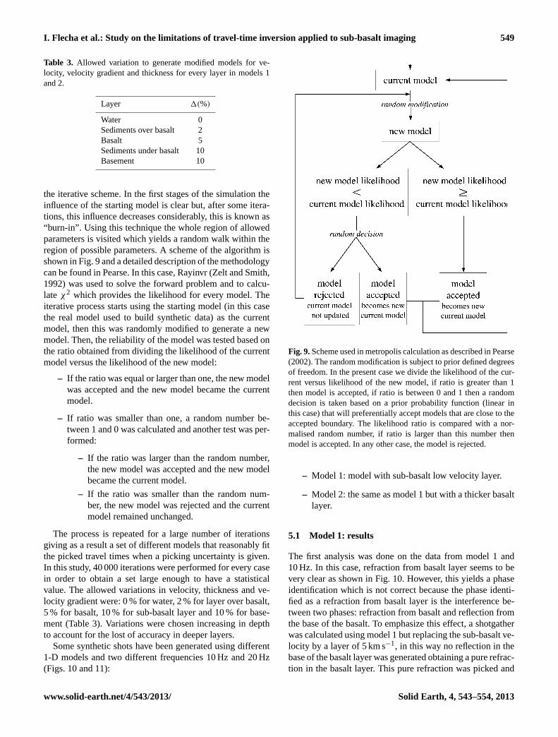
the iterative scheme. In the first stages of the simulation theinfluence of the starting model is clear but, after some itera-tions, this influence decreases considerably, this is known as“burn-in”. Using this technique the whole region of allowedparameters is visited which yields a random walk within theregion of possible parameters. A scheme of the algorithm isshown in Fig.9and a detailed description of the methodologycan be found inPearse. In this case, Rayinvr (Zelt and Smith,1992) was used to solve the forward problem and to calcu-lateχ2 which provides the likelihood for every model. Theiterative process starts using the starting model (in this casethe real model used to build synthetic data) as the currentmodel, then this was randomly modified to generate a newmodel. Then, the reliability of the model was tested based onthe ratio obtained from dividing the likelihood of the currentmodel versus the likelihood of the new model:

– If the ratio was equal or larger than one, the new modelwas accepted and the new model became the currentmodel.

– If ratio was smaller than one, a random number be-tween 1 and 0 was calculated and another test was per-formed:

– If the ratio was larger than the random number,the new model was accepted and the new modelbecame the current model.

– If the ratio was smaller than the random num-ber, the new model was rejected and the currentmodel remained unchanged.

The process is repeated for a large number of iterationsgiving as a result a set of different models that reasonably fitthe picked travel times when a picking uncertainty is given.In this study, 40 000 iterations were performed for every casein order to obtain a set large enough to have a statisticalvalue. The allowed variations in velocity, thickness and ve-locity gradient were: 0 % for water, 2 % for layer over basalt,5 % for basalt, 10 % for sub-basalt layer and 10 % for base-ment (Table3). Variations were chosen increasing in depthto account for the lost of accuracy in deeper layers.

Some synthetic shots have been generated using different1-D models and two different frequencies 10 Hz and 20 Hz(Figs.10and11):


Fig. 9. Scheme used in metropolis calculation as described in Pearse (2002). The random modification is subject to prior defined degrees offreedom. In the present case we divide the likelihood of the current versus likelihood of the new model, if ratio is greater than 1 then modelis accepted, if ratio is between 0 and 1 then a random decision is taken based on a prior probability function (linear in this case) that willpreferentially accept models that are close to the accepted boundary. The likelihood ratio is compared with a normalised random number, ifratio is larger than this number then model is accepted. In any other case, the model is rejected.

Fig. 9.Scheme used in metropolis calculation as described inPearse(2002). The random modification is subject to prior defined degreesof freedom. In the present case we divide the likelihood of the cur-rent versus likelihood of the new model, if ratio is greater than 1then model is accepted, if ratio is between 0 and 1 then a randomdecision is taken based on a prior probability function (linear inthis case) that will preferentially accept models that are close to theaccepted boundary. The likelihood ratio is compared with a nor-malised random number, if ratio is larger than this number thenmodel is accepted. In any other case, the model is rejected.

– Model 1: model with sub-basalt low velocity layer.

– Model 2: the same as model 1 but with a thicker basaltlayer.

5.1 Model 1: results

The first analysis was done on the data from model 1 and10 Hz. In this case, refraction from basalt layer seems to bevery clear as shown in Fig.10. However, this yields a phaseidentification which is not correct because the phase identi-fied as a refraction from basalt layer is the interference be-tween two phases: refraction from basalt and reflection fromthe base of the basalt. To emphasize this effect, a shotgatherwas calculated using model 1 but replacing the sub-basalt ve-locity by a layer of 5 km s−1, in this way no reflection in thebase of the basalt layer was generated obtaining a pure refrac-tion in the basalt layer. This pure refraction was picked and



Fig. 10.1-D model used to generate synthetic data (top). Shots gen-erated using the model and different frequencies: 10 Hz (left) and20 Hz (right). Main phases were identified: sea bottom reflection(blue), top basalt reflection (green), basalt refraction (red), top base-ment reflection (yellow) and basement refraction (orange). Underthe top of the basalt no phases were picked within the water-wavecone because in real data this phases are difficult to identify.

Fig. 11. 1-D model used to generate synthetic data (top). Shotsgenerated using the model and different frequencies: 10 Hz (left)and 20 Hz (right). Main phases were identified: sea bottom reflec-tion (blue), top basalt reflection (green), basalt refraction (red), basebasalt reflection (purple), top basement reflection (yellow) and base-ment refraction (orange). Under the top of the basalt no phases werepicked within the water-wave cone because in real data this phasesare difficult to identify.

compared with the identified in the previous case (Fig.12).Thus, in the first case, we have identified an interference be-tween basalt refraction and base basalt reflection as a purerefraction which is erroneous.

Using the picks from the data obtained with model 1 inthe Metropolis approach with a high picking error (see Ta-ble 4) and considering 40 000 different cases, we obtained


Fig. 12. Basalt refraction picks for model with sub-basalt low velocity layer (red) and for a model without sub-basalt low velocity layer(cyan). In the case without sub-basalt low velocity layer the picks represent a pure refraction while in the other case, the phase that isidentified as a refraction is made by the basalt refraction interfering with the base basalt reflection.

Fig. 12.Basalt refraction picks for model with sub-basalt low veloc-ity layer (red) and for a model without sub-basalt low velocity layer(cyan). In the case without sub-basalt low velocity layer the picksrepresent a pure refraction while in the other case, the phase that isidentified as a refraction is made by the basalt refraction interferingwith the base basalt reflection.

an overestimation in both, velocity and thickness of the sub-basalt layer (Fig.13). By reducing the picking error (casewith low uncertainty) we would expect a better correlationbetween the more probable model and the theoretical one. Inpractice, under the same conditions but reducing the pickinguncertainty, a worse result was obtained where there was noneed of a sub-basalt low velocity layer in order to fit the data(Fig. 14). This effect can be explained because considering abigger error in the picks, the range of times can include both,refraction within the basalt and reflection from the base ofthe basalt. Therefore, what was labelled as basalt refraction iswithin the allowed range of times for this phase. On the otherhand, by reducing the picking error, the range of times do notinclude the real refraction and then our erroneous phase iden-tification yields the unexpected result of Fig.14.

The same analysis was repeated using model 1 and datagenerated with 20 Hz. In this case, results are better and fitthe right model (Fig.15).

5.2 Model 2: results

In model 2 the thickness of basalt layer was increased totest if it was possible to use a well identified base basalt re-flection to constrain better the thickness and velocity of thislayer. Two different simulations have been performed: oneusing a very conservative picking and avoiding picks in the“interference zone” (basalt refraction/base basalt reflection)displayed in Fig.12 and another including more picks. Forthe first case (Fig.16) the velocity gradient for basalt layerwas well reproduced while for the second case (Fig.17) thisgradient did not fit the real model. For the basement veloc-ity gradient the result was the opposite, obtaining a betterresult when considering a larger number of picks. In both



Table 4.Picking uncertainty in ms for every layer considered in metropolis algorithm.

Phase model1 10 Hz model1 20 Hz model2 10 Hz model2 20 Hz

Seabed reflection 8 8 8 8 8Top basalt reflection 24 16 16 24 16Basalt refraction 50 24 24 50 24Top basement reflection 100 50 50 100 50Basement refraction 100 50 50 100 50

Figure 13 14 15 16,17 18

Fig. 13. Results obtained after using the Metropolis algorithm ondata from model 1 and 10 Hz for 40 000 cases. Red line representsthe real model and every black line a modified model. The colourscale stands for the number of times that a model (or part of it) isvisited. The preferred model (blue colours) overestimates the sub-basalt layer thickness as well as the velocity for this layer.

cases, sub-basalt velocity layer is not reliably recovered. Asin model 1, better fit is obtained for 20 Hz data (Fig.18),where the velocity gradient for basalt and basement are wellreproduced. Again, in both cases, the sub-basalt layer is notwell recovered.

The Metropolis study reveals that the phase identificationis a critical step. Despite objectivity provided by mathemat-ics used in the inversion, phase identification turns traveltime tomography in a subjective procedure. Additionally, un-certainty is also a critical parameter in the inversion whichcan influence the inversion algorithm. Moreover, consider-ing data with different frequency content also has an effecton the selection of the most probable model. Not all mod-els required a low velocity layer and there was an unresolv-able trade-off between thickness and velocity, even for mod-els where the base basalt reflection could be identified.

Fig. 14. Results obtained after using the Metropolis algorithm ondata from model 1 and 10 Hz for 40 000 cases. Uncertainties werereduced in comparison with the previous case (Fig.13). Red linerepresents the real model and every black line a modified model.The colour scale stands for the number of times that a model (or partof it) is visited. The preferred model consists in a velocity gradientwhich includes basalt, and basement layers, avoiding the need of alow velocity layer under the basalt.

Synthetic shots were created using a full-waveform codewhile likelihood was calculated using a ray tracing code.Full-waveform techniques are more accurate than ray tracingmethods because they take into account information aboutthe amplitudes, which are ignored in ray tracing simula-tions. Due to the high computational cost of full-waveformmethodologies, ray tracing methods are still conventionallyused to obtain velocity models (Pratt et al., 1996). These re-sults suggest that conventional travel time inversion (tomog-raphy) schemes without additional information are not suffi-cient to constrain the base of basalt or sub-basalt geologicalstructures.

In the synthetic tests performed in this study no noise hasbeen considered. In this sense, some features that commonlyare present in real data as tidal noise, electrical noise andsome other effects affecting the quality of the data, havenot been included. Results derived from these tests must be



Fig. 15. Results obtained after using the Metropolis algorithm ondata from model 1 and 20 Hz for 40 000 cases. Red line representsthe real model and every black line a modified model. The colourscale stands for the number of times that a model (or part of it) isvisited. The preferred model consists in a velocity gradient whichincludes basalt, sub-basalt and basement layers. The sub-basalt lowvelocity layer is reasonably well recovered in velocity and thick-ness.

Fig. 16. Results obtained after using the Metropolis algorithm ondata from model 2 and 10 Hz for 40 000 cases considering a “con-servative” picking avoiding picks in the “interference zone”. Redline represents the real model and every black line a modifiedmodel. The colour scale stands for the number of times that a model(or part of it) is visited.

Fig. 17. Results obtained after using the Metropolis algorithm ondata from model 2 and 10 Hz for 40 000 cases considering morepicks than in the previous case (Fig.16). Red line represents thereal model and every black line a modified model. The colour scalestands for the number of times that a model (or part of it) is visited.

Fig. 18. Results obtained after using the Metropolis algorithm ondata from model 2 and 20 Hz for 40 000 cases. Red line representsthe real model and every black line a modified model. The colourscale stands for the number of times that a model (or part of it) isvisited. The preferred model consists in a velocity gradient whichincludes basalt, sub-basalt and basement layers, avoiding the needof a low velocity layer under the basalt.



interpreted as results obtained in ideal conditions and in con-sequence, the best ones expected for a real case using thismethodology.

6 Conclusions

This study, which involves synthetic data suggests that thereare some physical limitations to obtain a reliable velocitymodel for sub-basalt zones in areas covered by high velocityrocks (like basalts and salts). In the case of thin basalt layers,the base basalt reflection is totally masked within the water-wave cone and it cannot be separated from the basalt refrac-tion. There are several subjective factors that can affect andcondition the results from the inversion as maximum pick-ing offset or picking uncertainty. Another important point isthe frequency content of the signal, our Metropolis simula-tions suggest that the original model is best recovered usinghigh frequencies and thicker basalt. This result is relevantbecause the actual tendency is using and designing airgunsthat produce low frequency data as single bubble source. Themost critical point in the travel time inversion is the phaseidentification/interpretation in the shot record. Differentiat-ing in the travel time branch, between the head wave trav-elling within the basalt (refraction) and, the base basalt re-flection is a key element in determining the correct thicknessof the basalt. The uncertainty associated to the travel timepicks is also a relevant issue, as it can not distinguish be-tween high and low velocity sub-basalt structures. Moreover,a wrong determination of the basalt thickness and velocityhas a direct influence on the resulting model for layers un-der the basalt. Reliable sub-basalt imaging with wide-anglereflection/refraction datasets requires additional informationas the knowledge on the thickness of the basalt at some pointand its internal velocity distribution. This could be achievedby using other methodologies to infer basalt properties.

Acknowledgements.Funding for this research was provided bySINDRI (Quantitative evaluation of the existing technologies forimaging within basalt-covered areas from the Faroes region), theSpanish Ministry of Science and Technology (Ref: CGL2004-04623/BTE) and Generalitat de Catalunya (Ref: 2005SGR00874).We are grateful to I. Trinks for training in the use of the TTT code.

Edited by: V. Sallares

References

Böhm, G. and Vesnaver, A.: Relying on a grid, J. Seism. Explor., 5,169–184, 1996.

Carmichael, R. S.: Handbook of Physical Properties of rocks, Vol.II, CSC Press, Boston, 1982.

Cervený, V.: Seismic Ray Theory, Cambridge Univ. Press, Cam-bridge, 2001.

Christensen, N. I. and Mooney, W. D.: Seismic velocity structureand composition of the continental crust: A global view, J. Geo-phys. Res., 100, 9761–9788, 1995.

Farra, V.: Amplitude computation in heterogenous media by raypertur- bation theory: a finite element approach, Geophys. J. Int.,103, 341–354, 1990.

Flecha, I., Martí, D., Carbonell, R., Escuder-Viruete, J., and Pérez-Estaún, A.: Imaging low velocity anomalies with the aid of seis-mic tomography, Tectonophysics, 388, 225–238, 2004.

Fliedner, M. M. and White, R. S.: Depth imaging of basalt flows inthe Faeroe-Shetland Basin, Geophys. J. Int., 152, 353–371, 2003.

Goff, J. A. and Jordan, T. H.: Stochastic modeling of seafloor mor-phology: inversion of sea beam data for second-order statistics,J. Geophys. Res., 96, 13589–13608, 1988.

Hobro, J. W. D., Singh, S. C., and Minshull, A.: Three-dimensionaltomo- graphic inversion of combined reflection and refractionseismic travel time data, Geophys. J. Int., 152, 79–93, 2003.

Hobbs, R.: Sub-basalt imaging using low frequencies. Subbasaltimaging 911th April, 2002 Cambridge, UK Journal of Confer-ence Abstracts, 7, 152–155, 2002.

Hughes, S., Barton, P. J., and Harrison, D.: Exploration in theShetland-Faeroe Basin using densely spaced arrays of ocean-bottom seismometers, Geophysics, 63, 490–501, 1998.

Jegen-Kulcsar, M. and Hobbs, R. W.: Outline of a joint inversionof gravity, MT and seismic data, Ann. Soc. Sci. Færoensis, 43,163–167, 2005.

Jolley, D. W. and Bell, B. R.: The evolution of the North AtlanticIgneous Province and the opening of the NE Atlantic rift, Ge-ological Society, London, Special Publication 2002, 197, 1–13,2002.

Korenaga, J., Holbrook, W. S., Kent, G. M., Kelemen, P. B., De-trick, R. S., Larsen, H. C., Hopper, J. R., and Dahl-Jensen, T.:Crustal structure of the Southeast Greeenland margin from jointrefraction and reflection seismic tomography, J. Geophys. Res.,105, 21591–21614, 2000.

Martini, F. and Bean, C. J.: Interface scattering versus body scat-tering in sub-basalt imaging and application of prestack waveequation datuming, Geophysics, 67, 1593–1601, 2002.

Martini, F., Bean, C. J., Dolan, S., and Marsan, D.: Seismic im-age quality beneath strongly scattering structures and implica-tions for lower crustal imaging: numerical simulations, Geophys.J. Int., 145, 423–435, 2001.

Martí, D., Carbonell, R., Escuder-Viruete, J., and Pérez-Estaún, A.:Characterisation of a fractured granitic pluton: P- and s-wavesseismic tomography and uncertainty analysis, Tectonophysics,422, 99–114, 2006.

McCaughey, M. and Singh, S. C.: Simultaneous velocity and inter-face tomography of normal-incidence and wide-aperture seismictraveltime data, Geophys. J. Int., 131, 87–99, 1997.

Metropolis, N., Rosenbluth, A. W., Rosenbluth, M. N., and Teller,A. H.: Equation of state calculations by fast computing machines,J. Chem. Phys., 21, 1087–1092, 1953.

Muir, F. and Dellinger, J.: A practical anisotrophic system., StanfordExploration Project Reports, 44, 55–58, 1985.

Pearse, S.: Inversion and modelling of seismic data to assess theevolution of the Rockall Trough, PhD thesis, Cambridge Univer-sity, 2002.



Pratt, R. G., Song, Z. M., Williamson, P., and Warner, M.: Two-dimensional velocity models from wide-angle seismic data bywavefield inversion, Geophys. J. Int., 124, 323–340, 1996.

Pujol, J. and Smithson, S.: Seismic wave attenuation in volcanic 570rocks from VSP experiments, Geophysics, 56, 1441–1455, 1991.

Raum, T., Mjelde, R., Berge, A. M., Paulsen, J. T., Digranes, P., Shi-mamura, H., Shiobara, H., Kodaira, S., Larsen, V. B., Fredsted,R., Harrison, D. J., and Johnson, M.: Sub-basalt structures east ofthe Faroe Islands revealed from wide-angle seismic and gravitydata, Petrol. Geosci., 11, 291–308, 2005.

Richardson, K. R., Smallwood, J. R., White, R. S., Snyder, D. B.,and Maguire, P. K. H.: Crustal structure beneath the Faroe Is-lands and the Faroe-Iceland Ridge, Tectonophysics, 300, 159–180, 1995.

Richardson, K. R., White, R. S., England, R. W., and Fruehn, J.:Crustal structure east of the Faroe Islands: mapping sub-basaltsediments using wide-angle seismic data, Petrol. Geosci., 5, 161–172, 1999.

Rousseau, J. H. L., Calandra, H., and de Hoop, M. V.: Three-dimensional depth imaging with generalized screens: A salt bodycase study, Geophysics, 68, 1132–1139, 2003.

Sallarès, V., Charvis, P., Flueh, E. R., and Bialas, J.: Seismic struc-ture of Cocos and Malpelo Ridges and implications for hot spot-ridge interaction, J. Geophys. Res., 108, 5(1)–5(21), 2003.

Sava, P. and Biondi, B.: Wave-equation migration velocity analy-sis. II. Subsalt imaging examples, Geophys. Prosp., 52, 607–623,2004.

Smallwood, J. R., Towns, M. J., and White, R. S.: The structureof the Faeroe-Shetland Trough from integrated deep seismic andpotential field modelling, J. Geol. Soc., 158, 409–412, 2001.

Sochacki, J. S., Kubichek, R., George, J. H., Fletcher, W. R., andSmithson, S. B.: Absorbing boundary conditions and surfacewaves, Geophysics, 52, 60–71, 1987.

Sochacki, J. S., George, J. H., Ewing, R. E., and Smithson, S. B.:Interface conditions for acoustic and elastic wave propagation,Geophysics, 56, 168–181, 1991.

Sørensen, A. B.: Cenozoic basin development and stratigraphy ofthe Faroes area, Petrol. Geosci., 9, 189–207, 2003.

Staples, R. K., Hobbs, R. W., and White, R. S.: A comparisonbetween airguns and explosives as wide-angle seismic sources,Geophys. Prosp., 47, 313–339, 1999.

Trinks, I.: Traveltime tomography of densely sampled seismic data,PhD thesis, Cambridge University, 2003.

Trinks, I., Singh, S. C., Chapman, C. H., Barton, P. J., Bosch, M.,and Cherrett, A.: Adaptative traveltime tomography of denselysampled seismic data, Geophys. J. Int., 160, 925–938, 2005.

Vesnaver, A.: Towards the uniqueness of tomographic inversion so-lutions, J. Seism. Explor., 3, 323–334, 1994.

White, R. S., Christie, P. A. F., Kusznir, N. J., Roberts, A., Davies,A., Hurst, N., Lunnon, Z., Parkin, C. J., Roberts, A. W., Smith,L. K., Spitzer, R., Surendra, A., and Tymms, V.: iSIMM pushesfrontiers of marine seismic acquisition, First Break, 20, 782–786,2002.

White, R. S., Smallwood, J. R., Fliedner, M. M., Boslaugh, B.,Maresh, J., and Fruehn, J.: Imaging and regional distribution ofbasalt flows in the Faroe-Shetland Basin, Geophys. Prosp., 51,215–231, 2003.

Williamson, P.: Introduction, Geophys. Prosp., 53, 167–168, 2003.Zelt, C. A. and Smith, R. B.: Seismic traveltime inversion for 2-D

crustal velocity structure, Geophys. J. Int., 108, 16–34, 1992.Ziolkowski, A., Hanssen, P., Gatliff, R., Jakubowicz, H., Dobson,

A., Hampson, G., Li, X.-Y., and Liu, E.: Use of low frequenciesfor sub-basalt imaging, Geophys. Prosp., 51, 169–182, 2003.


Study on the limitations of travel-time inversion applied to sub...

Documents

Transcript of Study on the limitations of travel-time inversion applied to sub...