Study on Rigid-Flexible Coupling Effects of Floating ... · dynamic model is a higher-order dynamic...
13
Study on Rigid-Flexible Coupling Effects of Floating Offshore Wind Tur- bines CHEN Jia-hao a, c , HU Zhi-qiang b, *, LIU Ge-liang a , WAN De-cheng a, c a State Key Laboratory of Ocean Engineering, Shanghai Jiao Tong University, Shanghai 200240, China b School of Engineering, Newcastle University, Newcastle upon Tyne, NE1 7RU, UK c Collaborative Innovation Center for Advanced Ship and Deep-Sea Exploration, Shanghai Jiao Tong University, Shanghai 200240, China Received April 29, 2018; revised September 10, 2018; accepted November 15, 2018 ©2019 Chinese Ocean Engineering Society and Springer-Verlag GmbH Germany, part of Springer Nature Abstract In order to account for rigid-flexible coupling effects of floating offshore wind turbines, a nonlinear rigid-flexible coupled dynamic model is proposed in this paper. The proposed nonlinear coupled model takes the higher-order axial displacements into account, which are usually neglected in the conventional linear dynamic model. Subsequently, investigations on the dynamic differences between the proposed nonlinear dynamic model and the linear one are conducted. The results demonstrate that the stiffness of the turbine blades in the proposed nonlinear dynamic model increases with larger overall motions but that in the linear dynamic model declines with larger overall motions. Deformation of the blades in the nonlinear dynamic model is more reasonable than that in the linear model as well. Additionally, more distinct coupling effects are observed in the proposed nonlinear model than those in the linear model. Finally, it shows that the aerodynamic loads, the structural loads and global dynamic responses of floating offshore wind turbines using the nonlinear dynamic model are slightly smaller than those using the linear dynamic model. In summary, compared with the conventional linear dynamic model, the proposed nonlinear coupling dynamic model is a higher-order dynamic model in consideration of the rigid-flexible coupling effects of floating offshore wind turbines, and accord more perfectly with the engineering facts. Key words: floating offshore wind turbine, dynamic stiffening effect, nonlinear coupled dynamic model, DARwind Citation: Chen, J. H., Hu, Z. Q., Liu, G. L., Wan, D. C., 2019. Study on rigid-flexible coupling effects of floating offshore wind turbines. China Ocean Eng., 33(1): 1–13, doi: 10.1007/s13344-019-0001-0 1 Introduction In recent years, floating offshore wind turbines (FOWTs) have been receiving increasing attention due to their prominent advantages, such as steadier and stronger wind available resources, lower operational noise, reduced visual pollution and fewer space limitations (Karimirad et al., 2011; Bachynski and Moan, 2012; Pérez-Collazo et al., 2015; Ma et al., 2015). FOWTs are complex rigid-flexible coupled multi-body systems (Namik and Stol, 2010; Wang and Sweetman, 2013; Nejad et al., 2015). Moreover, be- cause the slender blades of an FOWT system typically work at a high rotational speed and are influenced by the motions of the floating platform, rigid-flexible coupled dynamic re- sponses of FOWT systems are more complicated than those of the fixed bottom wind turbines. Rigid-flexible coupled multi-body dynamics have re- ceived considerable attentions during the development of modern high-speed airplanes (Shabana, 1997; Bauchau, 2011). In the 1970s, Winfrey (1971) proposed the “kineto- elastodynamics” (KED) method to model the dynamic beha- viour of rigid-flexible coupled multi-body systems. In this method, the system is first modelled as a rigid multi-body system to calculate the motion and inertia forces on the sys- tem. Second, the inertia and external forces are applied to the flexible components of the system to calculate the de- formation and the motion of the flexible components. The KED method is a decoupled method with the linear structur- al dynamics and kinematics of a rigid multi-body system. Hence, the coupling effects between the flexible bodies and the large overall motions from rigid bodies were not con- sidered. Likins (1972) proposed the “hybrid-coordinate dy- namic model” to describe the dynamic behaviour of rigid- flexible coupled multi-body systems. In this method, the flexible deformation is described with respect to the local body-fixed frames; then, the configuration of the system can be described as a superposition of the motions of these China Ocean Eng., 2019, Vol. 33, No. 1, P. 1–13 DOI: 10.1007/s13344-019-0001-0, ISSN 0890-5487 http://www.chinaoceanengin.cn/ E-mail: [email protected] Foundation item: This work was financially supported by the Ministry of Industry and Information Technology of China (Grant No. [2016]546). *Corresponding author. E-mail: [email protected]
Transcript of Study on Rigid-Flexible Coupling Effects of Floating ... · dynamic model is a higher-order dynamic...
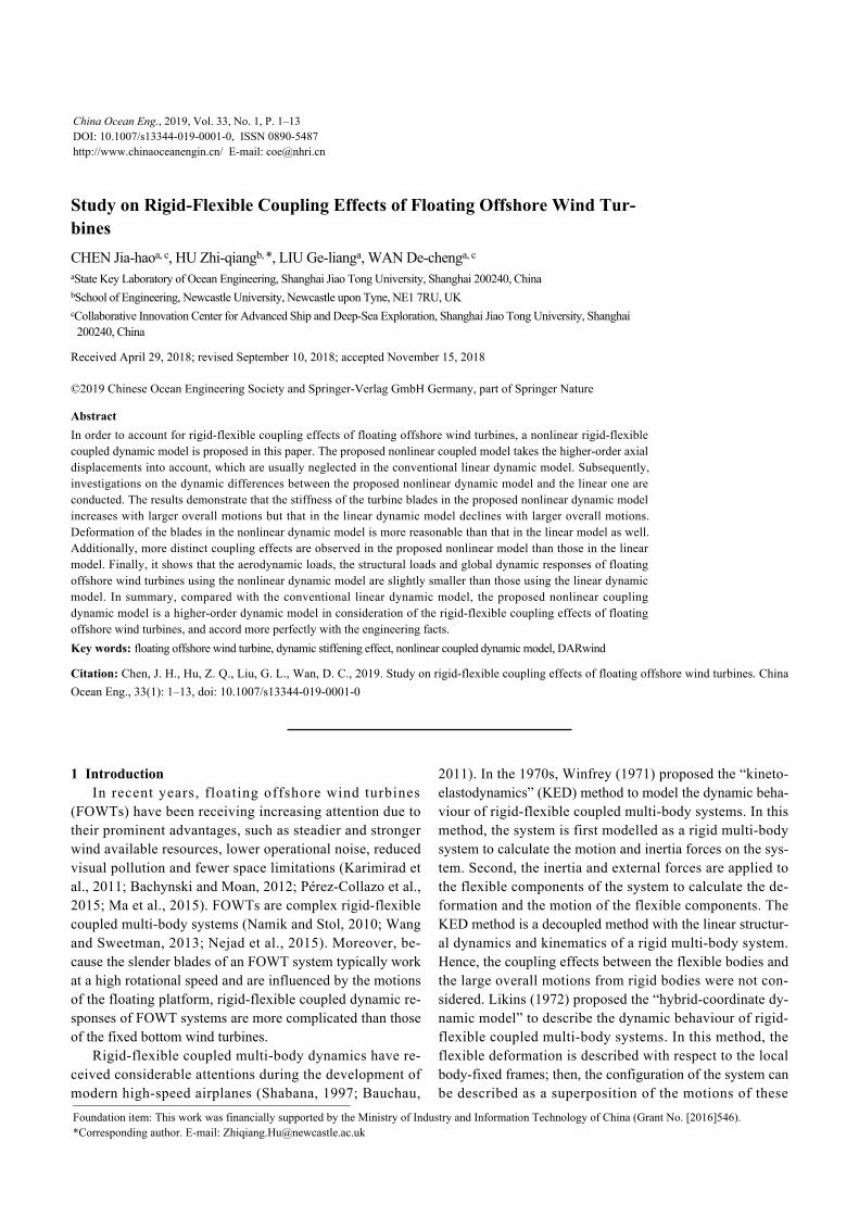
Study on Rigid-Flexible Coupling Effects of Floating Offshore Wind Tur-binesCHEN Jia-haoa, c, HU Zhi-qiangb, *, LIU Ge-lianga, WAN De-chenga, c
aState Key Laboratory of Ocean Engineering, Shanghai Jiao Tong University, Shanghai 200240, ChinabSchool of Engineering, Newcastle University, Newcastle upon Tyne, NE1 7RU, UKcCollaborative Innovation Center for Advanced Ship and Deep-Sea Exploration, Shanghai Jiao Tong University, Shanghai200240, China
Received April 29, 2018; revised September 10, 2018; accepted November 15, 2018
©2019 Chinese Ocean Engineering Society and Springer-Verlag GmbH Germany, part of Springer Nature
AbstractIn order to account for rigid-flexible coupling effects of floating offshore wind turbines, a nonlinear rigid-flexiblecoupled dynamic model is proposed in this paper. The proposed nonlinear coupled model takes the higher-order axialdisplacements into account, which are usually neglected in the conventional linear dynamic model. Subsequently,investigations on the dynamic differences between the proposed nonlinear dynamic model and the linear one areconducted. The results demonstrate that the stiffness of the turbine blades in the proposed nonlinear dynamic modelincreases with larger overall motions but that in the linear dynamic model declines with larger overall motions.Deformation of the blades in the nonlinear dynamic model is more reasonable than that in the linear model as well.Additionally, more distinct coupling effects are observed in the proposed nonlinear model than those in the linearmodel. Finally, it shows that the aerodynamic loads, the structural loads and global dynamic responses of floatingoffshore wind turbines using the nonlinear dynamic model are slightly smaller than those using the linear dynamicmodel. In summary, compared with the conventional linear dynamic model, the proposed nonlinear couplingdynamic model is a higher-order dynamic model in consideration of the rigid-flexible coupling effects of floatingoffshore wind turbines, and accord more perfectly with the engineering facts.Key words: floating offshore wind turbine, dynamic stiffening effect, nonlinear coupled dynamic model, DARwind
Citation: Chen, J. H., Hu, Z. Q., Liu, G. L., Wan, D. C., 2019. Study on rigid-flexible coupling effects of floating offshore wind turbines. ChinaOcean Eng., 33(1): 1–13, doi: 10.1007/s13344-019-0001-0
1 IntroductionIn recent years, floating offshore wind turbines
(FOWTs) have been receiving increasing attention due totheir prominent advantages, such as steadier and strongerwind available resources, lower operational noise, reducedvisual pollution and fewer space limitations (Karimirad etal., 2011; Bachynski and Moan, 2012; Pérez-Collazo et al.,2015; Ma et al., 2015). FOWTs are complex rigid-flexiblecoupled multi-body systems (Namik and Stol, 2010; Wangand Sweetman, 2013; Nejad et al., 2015). Moreover, be-cause the slender blades of an FOWT system typically workat a high rotational speed and are influenced by the motionsof the floating platform, rigid-flexible coupled dynamic re-sponses of FOWT systems are more complicated than thoseof the fixed bottom wind turbines.
Rigid-flexible coupled multi-body dynamics have re-ceived considerable attentions during the development ofmodern high-speed airplanes (Shabana, 1997; Bauchau,
2011). In the 1970s, Winfrey (1971) proposed the “kineto-elastodynamics” (KED) method to model the dynamic beha-viour of rigid-flexible coupled multi-body systems. In thismethod, the system is first modelled as a rigid multi-bodysystem to calculate the motion and inertia forces on the sys-tem. Second, the inertia and external forces are applied tothe flexible components of the system to calculate the de-formation and the motion of the flexible components. TheKED method is a decoupled method with the linear structur-al dynamics and kinematics of a rigid multi-body system.Hence, the coupling effects between the flexible bodies andthe large overall motions from rigid bodies were not con-sidered. Likins (1972) proposed the “hybrid-coordinate dy-namic model” to describe the dynamic behaviour of rigid-flexible coupled multi-body systems. In this method, theflexible deformation is described with respect to the localbody-fixed frames; then, the configuration of the system canbe described as a superposition of the motions of these
China Ocean Eng., 2019, Vol. 33, No. 1, P. 1–13DOI: 10.1007/s13344-019-0001-0, ISSN 0890-5487http://www.chinaoceanengin.cn/ E-mail: [email protected]
Foundation item: This work was financially supported by the Ministry of Industry and Information Technology of China (Grant No. [2016]546).*Corresponding author. E-mail: [email protected]

body-fixed frames and the flexible deformation with re-spect to these body-fixed frames. This method accounts forthe coupling effects between the flexible bodies and thelarge overall motions of the rigid bodies to some extent.However, the hybrid-coordinate dynamic model above is alinear method in fact, and certain higher-order quantities areneglected, which may cause some inaccurate dynamic res-ults under large overall motions. Kane et al. (1989) studiedthe dynamic behaviour of a cantilever beam attached to amoving boundary and found that the deformation of thebeam in the linear hybrid-coordinate dynamic model wouldtend toward infinity with the increasing rotational speed,which contradicted the reality that the stiffness of a canti-lever beam should increase with the increasing rotationalspeed. Kane firstly proposed “dynamic stiffening” to de-scribe this phenomenon. Other experiments also demon-strated significant coupling effects between the flexible bod-ies and the large overall motions (Lee et al., 2001; Santos etal., 2004). Since then, coupling effects and the defects of thelinear dynamic model have attracted considerable attention.Although several researchers have corrected the linear dy-namic model to successfully detect dynamic stiffening ef-fects in a rigid-flexible coupled multi-body system usingdifferent methods (Banerjee and Dickens, 1990; Liu andLiew, 1994; Mayo et al., 1995; Sharf, 1995), there is still nowidespread consensus regarding the essence of these coup-ling effects. The omission of the higher-order strain-dis-placement relationship in the linear dynamic model could bethe reason for the failure to model dynamic stiffening ef-fects in a rigid-flexible coupled multi-body system (Mayo etal., 1995). After investigating the dynamic characteristics ofa cantilever beam attached to a moving base, Liu and Hong(2003, 2004) found that the inaccuracy in the linear dynam-ic model is caused by the omission of the axial foreshorten-ing displacement induced by the lateral displacements whenundergoing large overall motions.
In the wind energy field, researchers (Lee et al., 2002;Santos et al., 2004; Larsen and Nielsen, 2006) have foundthat these coupling effects are important for the blades offixed-bottom wind turbines as well. Compared with fixed-bottom wind turbine systems, FOWTs are the relatively newconcept and their blades are slenderer and the six-degree-of-freedom (DOF) motion of the floating platform usuallygives rise to large overall motions of the blades. Thus, non-linear rigid-flexible coupling effects in FOWTs are moredistinct, but the related researches are scarce.
The purpose of this study is to propose an appropriate ri-gid-flexible coupling dynamic model and to investigate thecoupling rigid-flexible effects of the floating wind turbinesystem. Hence, the work of the paper includes:
(1) Deducing a nonlinear coupling dynamic model ap-plied to the FOWTs modelling.
(2) Comparing dynamic differences between the pro-posed nonlinear dynamic model and the linear one in an
FOWT system.(3) Investigating rigid-flexible coupling effects of an
FOWT system.In view of the fact that the movement of the foundation
of the tower is relatively small and the deformation of theshaft is negligible, thus, the tower is modeled as a linearmodel and the shaft is modeled as a rigid body. In otherwords, the nonlinear rigid-flexible modeling is only appliedto the blades. This paper makes contribution for a better un-derstanding of the rigid-flexible coupled dynamic effects ofan FOWT system and hopes to raise awareness of this issuein the FOWTs research community.
2 Theories and methodologyIn this section, the theories on the linear dynamic model
and the proposed nonlinear coupled dynamic model are in-troduced in details. First, the fundamental kinematic meth-od is presented. Subsequently, the dynamic governing equa-tion for a three-dimensional flexible beam undergoing largeoverall motions is deduced to compare the essential distinc-tion between the linear dynamic model and the nonlinearcoupled dynamic model.
2.1 Kinematics description
e0
eb
The “floating frame of reference formulation” method(Nada et al., 2010; Nowakowski et al., 2012; Held et al.,2016) is used to describe the kinematics of an FOWT sys-tem. In this method, there are two sets of coordinate frames.One is the global reference frame (RF), which describes thelocation and the orientation of the bodies, and the other isthe local elastic body-fixed frame (BF), which describes theelastic deformation of flexible bodies. This method isschematically illustrated in Fig. 1, where is the globalreference coordinate frame (RF) and is the local body-fixed coordinate frame (BF).
eb(t)ρP0
∆U
The position of an arbitrary point P with respect to thebody-fixed frame in the undeformed state is denoted as
. The deformation of this point is defined as . Hence,the position vector of Point P after deformation with re-
Fig. 1. Floating reference frame.
2 CHEN Jia-hao et al. China Ocean Eng., 2019, Vol. 33, No. 1, P. 1–13

eb(t)spect to is written as follows:ρP = ρP0
+∆U. (1)
e0The position vector of Point P after deformation with re-
spect to the global reference frame is written as follows:rP = rb+ρP . (2)
Substituting Eq. (1) into Eq. (2) yields:rP = rb+ρP0
+∆U. (3)
rP
According to Eq. (3), the velocity vector of Point P isthe first derivative of the position vector , written as fol-lows:
rP = rb+ω×(ρP0+∆U
)+∆U, (4)
ωe0 ∆U
eb(t) ×
where is the instantaneous angular velocity vector of thebody with respect to , denotes the first-order derivat-ive of the deformation versus time with respect to the localbody-fixed frame and the symbol indicates the crossproduct.
e0Based on Eq. (4), the acceleration vector of Point P with
respect to the global reference frame is written as fol-lows:
rP =rb+ ω×(ρP0+∆U
)+2ω×∆U+ω×[
ω×(ρP0+∆U
)]+∆U, (5)
∆U
eb(t)
where denotes the second-order derivative of the de-formation versus time with respect to the local body-fixedframe .
∆UIn order to describe the deformation in a rigid-flex-ible coupled multi-body system, Likins (1972) proposed thelinear hybrid-coordinate dynamic model. In this method, thekinematic relationship between rigid and flexible bodies isdescribed by the floating frame of the reference formulationdescribed above, and the flexible deformation is based onthe small deformation assumption, in which the geometric-ally nonlinear quantities are neglected to linearize the de-formation field. However, the neglected certain geometric-ally nonlinear quantities in this linear dynamic model maybe significant for a rigid-flexible coupled multi-body sys-tem undergoing large overall motions. Therefore, the studyin this paper proposes a nonlinear dynamic model in consid-eration of these geometrically nonlinear high-order quantit-ies in a rigid-flexible coupled multi-body system. In the fol-lowing sections, the linear dynamic model presented aboveis denoted “L-model” (low-order model), and the proposednonlinear dynamic model is denoted “H-model” (higher-or-der model).
2.2 Dynamic governing equationsIn this subsection, the dynamic governing equation for a
three-dimensional flexible beam with large overall motionsis deduced. In addition, the essential difference between thelinear dynamic model and the proposed nonlinear dynamicmodel will be discussed.
Ob− bexbey
bez
ωk0 x
k0
k Uk
Because the blades of an FOWT are slender and at-tached to a hub, the blades can be modeled as anEuler–Bernoulli cantilever beam attached to a movable ri-gid boundary. For simplicity, in the following sections, thecantilever beam is homogeneous and isotropic, and thecentroid axis of the cross section along the beam is also co-incident. A three-dimensional Euler–Bernoulli cantileverbeam with large overall motions is shown in Fig. 2, where
is the local body-fixed frame of the canti-lever beam. The hub rotates at an angular velocity . Point
is at the position along the undeformed neutral axis ofthe beam. After deformation, Point moves to a new posi-tion . is the deformation vector of the point and can bewritten as:
Uk =
[ ux0uy0uz0
](6)
ux0 uy0 uz0
Ukbex
beybez
where , and are the coordinate components of de-formation along the coordinate axes , and , re-spectively.
Assuming that the length of a differential element at theposition x is dx before deformation, the stretch of this ele-ment along the neutral axis after deformation can be writtenas:
ds =
√(1+
dux0
dx
)2
+
(duy0
dx
)2
+
(duz0
dx
)2
·dx (7)
ε0Hence, the axial normal strain is:
ε0 =ds−dx
dx. (8)
Substituting Eq. (7) into Eq. (8), and then expanding theequation by the Taylor expansion yields:
ε0 ≈dux0
dx+
12
(duy0
dx
)2
+
(duz0
dx
)2 . (9)
kx
According to Eq. (9), the stretch of the beam at Point can be obtained by an integral from zero to the position :
w1 =w x
0ε0dx = ux0+
12
w x
0
(duy0
dx
)2
+
(duz0
dx
)2dx. (10)
Let
Fig. 2. Three-dimensional cantilever beam with large overall motions.
CHEN Jia-hao et al. China Ocean Eng., 2019, Vol. 33, No. 1, P. 1–13 3

wg = −12
w x
0
(duy0
dx
)2
+
(duz0
dx
)2dx, (11)
and thus,ux0 = w1+wg. (12)
wgbex
uy0 uz0
Eq. (11) indicates that is an axial foreshortening dis-placement along caused by the coupling effects from thelateral displacements and . Considering this fore-shortening displacement or not is the essential differencebetween the linear dynamic model (L-model) and the pro-posed nonlinear dynamic model (H-model).
bex
For an arbitrary point in the cross-section of a beam, anadditional axial displacement along caused by the cross-sectional rotation effect can be approximated as follows:
wr ≈ −y∂w2
∂x− z
∂w3
∂x. (13)
Hence, the deformation of an arbitrary point in the cross-section of an Euler-Bernoulli cantilever beam is written as:
U =[ ux0
uy0uz0
]=
[ w1+wg+wrw2w3
], (14)
w1 w2 w3
wg wr
where is the stretch along the neutral axis, and and are the lateral displacements induced by the bending deflec-tions with respect to the body-fixed frame. and are thelateral-displacement-induced axial displacement and sec-tion-rotation-induced axial displacement, respectively.
ux0
By substituting Eqs. (11) and (13) into Eq. (14), the x-axis displacement (see Fig. 2) can be written as:ux0 =w1+wg+wr = w1−
12
w x
0
(duy0
dx
)2
+
(duz0
dx
)2dx− y∂w2
∂x− z
∂w3
∂x. (15)
According to Eq. (9) and Eq. (15), the strain power ofthe beam can be approximated as follows:
V =w L
0
wAσdAεdx ≈
w L
0EA
(∂w1
∂x
)(∂w1
∂x∂t
)dx+
w L
0EIzz
(∂2w2
∂x2
)(∂2w2
∂x2∂t
)dx+
w L
0EIyy
(∂2w3
∂x2
)(∂2w3
∂x2∂t
)dx,
(16)Izz =
rA y2dA Iyy =
rA z2dA
E A
where and are the central princip-al second moments of the area with respect to the z-axis andy-axis, respectively; is Young’s modulus and is thecross-sectional area.
In this paper, the modal superposition method (Andr-eaus et al., 2016) is used to disperse the beam model. Thus,axial and lateral deformation can be dispersed as:
w1 =
n∑i=1
ϕxiqxi =ΦTx qx = qT
xΦx; (17)
w2 =
n∑i=1
ϕyiqyi =ΦTy qy = qT
yΦy; (18)
w3 =
n∑i=1
ϕziqzi =ΦTz qz = qT
zΦz, (19)
ϕxi ϕyi ϕziqxi qyi qzi
bexbey
bez
w (0) = 0w′ (0) = 0
w′′ (L) = 0w′′′ (L) = 0
where , and are the i-th spatial shape functions and, and are the i-th generalized coordinates with re-
spect to the coordinate axes , and of the localbody-fixed frame, respectively. A cantilevered boundarycondition is used for the beam model, in other words, thebase of the beam does not experience any deflection
, the derivative of the deflection function at thatpoint is zero , there is no bending moment at thefree end , and there is no shearing force acting atthe free end .
In regard to blades mode order, Øye (1996) found thatthe first 3 or 4 eigenmodes (2 flapwise eigenmodes, 1 or 2edgewise eigenmodes) used for a wind turbine are in goodagreement with the measurements. Thus, the first 3 eigen-modes (2 flapwise eigenmodes and 1 edgewise eigenmode)are used to disperse the blades in the subsequent tests. Spa-tial shape functions for the blades are approximated as 6th-order polynomials calculated by the preprocessor Mode(Marshall, 2002), as shown in Fig. 3.
According to Eq. (14), the deformation of an arbitrarypoint in the cross-section and its first and second derivat-ives are written as follows:
U =(Φ+
12
ATQH+R
)Q; (20)
U =(Φ+ AT
QH+R)Q; (21)
U =(Φ+ AT
QH+R)Q+ AT
QHQ, (22)
whereSpatial shape functions matrix:
Φ =
ΦTx 0 0
0 ΦTy 0
0 0 ΦTz
,Φx =
[ ϕx1 ϕx2 · · · ϕxn]
Φy =[ϕy1 ϕy2 · · · ϕyn
]Φz =
[ ϕz1 ϕz2 · · · ϕzn] (23)
Generalized coordinate matrix:
Fig. 3. Spatial shape functions of the blades.
4 CHEN Jia-hao et al. China Ocean Eng., 2019, Vol. 33, No. 1, P. 1–13

Q = qx
qyqz
,
qx = [ qx1 qx2 · · · qxn ]qy = [ qy1 qy2 · · · qyn ]qz = [ qz1 qz2 · · · qzn ]
(24)
AQ = [ Q 0 0 ] (25)Cross-sectional rotation effect matrix:
R =
0 −y(∂ϕy
∂x
)T
−z(∂ϕz
∂x
)T
0 0 00 0 0
(26)
Nonlinear coupling effect matrix:
H =
0 0 00 Hy 00 0 Hz
;
Hy = −w x
0
(∂ϕy
∂x
)·(∂ϕy
∂x
)T
dx;
Hz = −w x
0
(∂ϕz
∂x
)·(∂ϕz
∂x
)T
dx. (27)
Variational forms of the above terms are rewritten asfollows:
δU =(Φ+R+ AT
QH)·δQ; (28)
δU =(Φ+R+ AT
QH)·δQ+ AT
QH ·δQ. (29)
From Eq. (4), the velocity of an arbitrary point in thecross section in the variational form is:
δr = δrb−(ρP0 + U
)·δω+
(Φ+R+ AT
QH)·δQ. (30)
From Eq. (16), the virtual strain power of the beam iswritten as follows:
δV = δQTK0Q, (31)where
Constant stiffness matrix:
K0 =
[ Kx 0 00 Ky 00 0 Kz
],
Kx =w L
0EA
(∂ϕx
∂x
)(∂ϕx
∂x
)T
dx
Ky =w L
0EIzz
∂2ϕy
∂x2
∂2ϕy
∂x2
T
dx
Kz =w L
0EIyy
∂2ϕz
∂x2
∂2ϕz
∂x2
T
dx
(32)
Based on Jourdain’s variational principle (Jourdain,1909; Wang and Pao, 2003), the dynamic equation for theflexible cantilever beam with a movable boundary can bewritten as:
δW−wΩρδrT rdΩ−δV = 0, (33)
δW
δW = 0
where is the power of the virtual active forces. For sim-plicity in the following analysis, we assume that the beamvibrates without any active force ( ), and the beam
δrb = 0 δω = 0
R = 0
performs a specified motion; in other words, we can let thevariation and . For a slender beam (e.g., off-shore wind turbine blades), the transverse size is far smallerthan the axial size; thus, additional axial displacementscaused by the cross-sectional rotation effect can be neg-lected, . Substituting Eqs. (5), (30) and (31) into Eq.(33), we can obtain the dynamic governing equation of athree-dimensional flexible beam with large overall motions:
δQT{w
Ωρ(ΦT+HAQ
) [rb+ ˜ω
(ρP0+U
)+2ωU +
ωω(ρP0+U
)+ U
]dΩ+K0Q
}= 0, (34)
H = HT ρP0=
[xP 0 0
]T
δQT U U Uwhere , and . Eliminating theterm and then substituting , and (Eqs. (20), (21)and (22)) into Eq. (34) becomeswΩρ(ΦT+HAQ
) {(Φ+ AT
QH)Q+2ω
(Φ+ AT
QH)Q +[
˜ω(Φ+
12
ATQH
)+ ωω
(Φ+
12
ATQH
)]Q+(
rb+ ˜ωρP0+ ωωρP0
+ ATQHQ
)}dΩ+K0Q = 0. (35)
The above dynamic governing equation can be summar-ized as follows:
MQ+CQ+KQ+F = 0. (36)
In the linear dynamic model (L-model) for the beam,Eq. (36) is written as:
MLQ+CLQ+KLQ+FL = 0. (37)In the proposed nonlinear coupling dynamic model (H-
model), Eq. (36) is written as:
(ML+MH) Q+ (CL+CH) Q+ (KL+KH)Q+FL+FH = 0, (38)
whereMass matrix:
MQ =wΩρ(ΦT+HAQ
) (Φ+ AT
QH)dΩ · Q; (39)
ML =wΩρΦTΦdΩ; (40)
MH =wΩρHAQΦdΩ+
wΩρΦT AT
QHdΩ+wΩρHAQ AT
QHdΩ. (41)
Damping matrix:
CQ =wΩρ(ΦT+HAQ
)·2ω ·
(Φ+ AT
QH)dΩ · Q; (42)
CL = 2wΩρΦTωΦdΩ; (43)
CH =2wΩρΦTωAT
QHdΩ+2wΩρHAQωΦdΩ+
2wΩρHAQωAT
QHdΩ. (44)
Stiffness matrix:
CHEN Jia-hao et al. China Ocean Eng., 2019, Vol. 33, No. 1, P. 1–13 5

KQ =wΩρ(ΦT+HAQ
) [˜ω(Φ+
12
ATQH
)+ ωω
(Φ+
12
ATQH
)]dΩ ·Q+
wΩρ(HAQ
) (rb+ ˜ωρP0
+ ωωρP0
)dΩ+K0Q;
(45)
K = KL+KH; (46)
KL = K0+Kf ; (47)
Kf =wΩρΦTωωΦdΩ+
wΩρΦT ˜ωΦdΩ; (48)
KH =12
wΩρΦT ˜ωAT
QHdΩ+wΩρHAQ ˜ωΦdΩ+
12
wΩρHAQ ˜ωAT
QHdΩ+wΩρHAQωωΦdΩ+
12
wΩρΦTωωAT
QHdΩ+12
wΩρHAQωωAT
QHdΩ+wΩρ(
˜ωρP0
)1HdΩ+
wΩρ[(rb)1+
(ωωρP0
)1
]HdΩ,
(49)()1where the symbol denotes the first element of a matrix.
Additional generalized force terms:
FL =wΩρΦT rbdΩ+
wΩρΦT ˜ωρP0
dΩ+wΩρΦTωωρP0
dΩ;
(50)
FH =wΩρ(ΦT+HAQ
)AT
QHdΩ · Q, (51)
ω
where ~ notes a coordinate matrix of a vector, for example, is written as follows:
ω =
[ 0 −ω3 ω2ω3 0 ω1−ω2 ω1 0
](52)
Hω
˜ωrb
As illustrated in Eqs. (37) and (38), the L-model is a lin-ear model, but the H-model is a nonlinear higher-ordermodel. And the H-model contains additional mass terms,damping terms, stiffness terms and additional generalizedforce than the L-model. All of these additional terms in theH-model are relevant to the higher-order geometrically non-linear term . Moreover, some of them are relevant to thecoordinate matrix of the angular velocity , the coordinatematrix of the angular acceleration and the acceleration ofthe boundary . In other words, the additional terms in theH-model are influenced by the motions of the body, whichis more in accordance with the actual situation.
ω rb
ω1 ω2
Kf KH
KH
To simplify the following analysis, the angular accelera-tion term and the acceleration of the foundation areneglected (these quantities are typically much smaller thanthe angular velocities). Moreover, because the rotationalmotion of the blades is mainly along one axis, the othercomponents of the angular velocity (e.g., and ) are re-latively small and are neglected to simplify the followinganalysis. Therefore, the stiffness terms and (somesmall higher-order quantities are neglected in ) are sim-plified as follows:
Kf = −ω23ρ ·
wΩ
ϕxϕTx 0 0
0 ϕyϕTy 0
0 0 0
dΩ; (53)
KH ≈wΩρ
0 0 00 −ω2
3xPHy 00 0 −ω2
3xP Hz
dΩ =
ω23ρ
wΩ
xP
0 0 0
0w x
0
(∂ϕy
∂x
)·(∂ϕy
∂x
)T
dx 0
0 0w x
0
(∂ϕz
∂x
)·(∂ϕz
∂x
)T
dx
dΩ.
(54)Kf
KH
Eq. (53) shows that is negative and proportional tothe square of the angular velocity. In other words, the stiff-ness of the flexible bodies in the L-model declines and thedeformation is amplified with the rotational motion, whichis inconsistent with the reality (Lee et al., 2001; Santos etal., 2004). In contrast, as shown in Eq. (54), is positiveand increases with the square of the angular speed. In otherwords, the stiffness of the flexible bodies in the H-model in-creases with the rotational motion, which is more in linewith the reality (Lee et al., 2001; Santos et al., 2004). Thedifference in the stiffness between the two modelling meth-ods likely causes other differences in the dynamic beha-viours in a rigid-flexible multi-body system. Moreover, asshown in Eq. (38), the H-model contains additional massterms, damping terms, stiffness terms and generalized forceterms. These additional terms likely also give rise to differ-ences in the dynamic behaviour of a rigid-flexible coupledmulti-body system between the two models. Detailed in-vestigations and comparisons between the two modellingmethods are conducted in the subsequent sections.
The aforementioned linear dynamic model and the non-linear coupled dynamic model were both incorporated intoour in-house aero-hydro-servo-elastic coupled FOWT simu-lation code DARwind to simulate the time-domain coupleddynamic behaviours of an FOWT system. In this section,the theories of the numerical program DARwind are brieflyintroduced.
(1) Aerodynamics (Hansen, 2015): The blade elementmomentum (BEM) method is used to calculate the aerody-namic loads. Several corrections are also considered, suchas the Prandtl’s blade-tip loss, hub-loss, the Glauert’s cor-rection, the skewed wake correction and the dynamic wakecorrection. The solution to the aerodynamic inductionfactors iterates until it converge to reasonable values.
(2) Hydrodynamics (Faltinsen, 1990; Newman, 1997):Airy linear wave theory, the potential flow theory and Mor-ison’s formula are applied to calculate the hydrodynamicloads. Hydrodynamic parameters are calculated by a pre-processor WAMIT. Subsequently, these frequency-domainhydrodynamic coefficients are taken as input data and con-
6 CHEN Jia-hao et al. China Ocean Eng., 2019, Vol. 33, No. 1, P. 1–13

verted to the time-domain hydrodynamic loads in DAR-wind. Morison’s formula is used to correct the flow-separa-tion-induced nonlinear viscous drag on the floating plat-form.
(3) Mooring lines (Masciola et al., 2013): A quasi-staticapproach for a catenary mooring system is used in the code.The stretching of a mooring line is considered, but certaindynamic characteristics (e.g., the inertia, damping and bend-ing) of the mooring system are neglected.
(4) Control system (Jonkman, 2007): Controllerstrategies consist of a generator-torque controller and a full-span rotor-collective blade-pitch controller. The generator-torque controller is mainly used to maximize the power cap-ture below the rated wind speed. The blade-pitch controlleris mainly used to regulate the generator speed and electricalpower above the rated wind speed.
(5) Kinetics (Kane and Levinson, 1983; Huston andJames, 1982): Kane’s dynamic equations are used to estab-lish the dynamic governing equations of an FOWT system.The adjacent array method is applied to describe the topolo-gical relation between the bodies of an FOWT system. Themodal superposition method is applied to discretize the flex-ible bodies (e.g., blades and tower). The aforementioned lin-ear dynamic model and the nonlinear coupled dynamicmodel are considered in the dynamic equations.
The code DARwind was developed using the above the-ories to model the time-domain coupled dynamic beha-viours of an FOWT system. Compared with the other exist-ing softwares, DARwind is more convenient to simulateFOWTs as different models. For example, the FOWT sys-tem can be modeled as a single rigid body system for lesstime cost, modeled as a multi-rigid-body system for a bal-ance of the time cost and computational accuracy, ormodeled as a rigid-flexible coupling multi-body system withor without considering nonlinear rigid-flexible coupled ef-fects for accurate simulations but most time consuming.More details about the theories and verification of DAR-wind code can be found in Refs. (Hu et al., 2017; Chen etal., 2019).
3 Results and discussionTests (see Table 1) are conducted to compare differ-
ences between the H-model and L-model and to clarify thesignificance of the rigid-flexible coupling effects in an
Hs Tp
γ
FOWT system. The floating platform is fixed to eliminatethe influence from the 6-DOF motion of the floating plat-form for certain test cases (e.g., T1, T2, and T3). For thecases T4 and T6, the platform is moored by three catenarymooring lines. For T5, the floating platform moves in a spe-cified manner regardless of external forces. The wave con-ditions are based on the JONSWAP wave spectrum with asignificant wave height , a peak period , and a peak en-hancement factor .
O0− x0y0z0
O0
O1−x1y1z1
Ob− xbybzb
xb zb
In the following tests, an OC4 semi-submersible FOWT(Robertson et al., 2014) is selected as the test object, inwhich the NREL-5MW reference wind turbine is used(Jonkman et al., 2009). Main properties of the OC4 semi-submersible FOWT are listed in Table 2. The constructionof the OC4 semi-submersible FOWT are shown in Fig. 4.As shown in Fig. 4a, is the global inertial frameand the origin is located at the intersection between thestill water surface and the initial tower centreline. is the body-fixed frame of the floating platform, which ini-tially coincides with the frame of global inertial frame.
is the local body-fixed frame of each blade,fixed at the blade root (see Fig. 4b). The positive directionof the -axis points to the nacelle and the -axis is alongthe neutral axis of the blade, which is different from Fig. 2.
3.1 Dynamic stiffening effect and influencing factorsThis subsection investigates the relationship between the
rotational speed and bending stiffness of the blades for thetwo models (L-model and H-model). Calculations are con-ducted for the test case T1 (see Table 1). In T1, the support-ing platform is fixed, and the rotor rotates at different rota-tional speeds without suffering from aerodynamic loads.The first natural frequencies of the blades in flapwise andedgewise modes under different rotational speeds are listedin Table 3 and plotted in Fig. 5. The results are comparedwith those calculated by FAST (Jonkman et al., 2005; Jonk-man, 2007). Table 3 and Fig. 5 show that the results calcu-lated by Darwind (H-model) and FAST are in good consist-ency. More comparisons on the dynamic responses betweenthese two codes can be found in the reference (Hu et al.,2017).
Comparing the results calculated by the H-model and L-model (see Table 3 and Fig. 5), we know that the flapwisenatural frequency of the L-model’s blades is nearly con-
Table 1 Test case matrixTest case Platform state Vwind (m/s) Wave condition Ω (rmp) BtDef (m)
T1 Fixed 0.00 Still water 0–30 0.0T2 Fixed 11.4 Still water 12.1 0.0T3 Fixed 11.4 Still water 20.0 0.0T4 Moored 0.00 Still water 0.00 4.0T5 Specified 0.00 Still water 0.00 1.0T6 Moored 11.4 Irregular wave 12.1 0.0
ΩHs=2 m Tp=8 s γ=3.3
Notes: “Vwind” represents the steady wind speed; “ ” represents the rotor speed; “BtDef” denotes the initial deformation at the blade tips. Irregular wavecondition: , , .
CHEN Jia-hao et al. China Ocean Eng., 2019, Vol. 33, No. 1, P. 1–13 7

stant under different rotational speed conditions and theedgewise frequency in the L-model declines with the rota-tional speed. It is consistent with Eq. (53) in that the out-of-plane (flapwise) stiffness of the L-model is not influencedby the rotational speed, but the in-plane (edgewise) stiff-ness declines and is even negative when the rotational speedexceeds its fundamental natural frequency. In contrast, inthe H-model, the natural frequency of the blades increaseswith the rotational speed in both the flapwise and edgewisemodes. In other words, the stiffness of the H-model’s blades
increases with the rotational speed, which is in accordancewith Eq. (54). Relevant experiments (Lee et al., 2001; San-tos et al., 2004) have also proved that flexible bodies stiffenwhen undergoing large rotational motions and the stiffen-ing effects increase with the rotational speed, which is theso called “dynamic stiffening effect” (Liu and Hong, 2003).On the other hand, Cai et al.(2005) found that a numericaldivergence might appear using the linear dynamic model (L-model) when the rotational speed of the flexible beam isclose to or exceeds its fundamental natural frequency. For-tunately, the operating rotational speed of the wind turbineblades is generally much smaller than the fundamental nat-ural frequency.
The above analysis demonstrates that the stiffness of theblades in the H-model and L-model are different, and thegap even increases with the blades rotational speed. The dif-ferences likely introduce dynamic differences between thetwo models, e.g., aerodynamic loads, structural loads andblade deflection. Thus, the test case T2 (see Table 1) was
Table 2 Main properties of an OC4 semi-submersible FOWTProperty Values
Rated power 5 MWRated wind & rotor speed 11.4 m/s, 12.1 rpm
Rotor type Upwind, 3 bladesRotor diameter 126 mTower height 77.6 mPlatform type SemisubmersibleWater depth 200 m
Mooring system 3 lines, catenary
Table 3 First natural frequency of the blades in the two models
Rotor speed(rad/s)
Flapwise (x) (rad/s) Edgewise (y) (rad/s)
FASTDarwind
FASTDarwind
H L H L0.000 4.41577 4.43970 4.41896 6.80595 6.89014 6.890140.722 4.50996 4.52327 4.41896 6.84829 6.91088 6.848040.942 4.56353 4.58610 4.41896 6.84836 6.91088 6.827311.267 4.70993 4.73312 4.41896 6.86878 6.93161 6.764482.094 5.21296 5.23515 4.41896 6.95278 7.01580 6.554623.140 6.06013 6.09406 4.41896 7.12011 7.20430 6.13616
Fig. 4. Overview of an OC4 semi-submersible FOWT.
Fig. 5. First natural frequency of the blades in the two models.
8 CHEN Jia-hao et al. China Ocean Eng., 2019, Vol. 33, No. 1, P. 1–13

conducted to compare the dynamic responses between thetwo models, and the test results are listed in Table 4. Com-paring the results calculated by the H-model and the L-mod-el (see Table 4), we know that the lateral blade-tip deforma-tions in the H-model are smaller than those in the L-model.In addition, there is an axial foreshortening displacement inthe H-model but that keeps zero in the L-model. For thestructural loads at the blade root, the mean shear force andbending moment of the H-model is slightly smaller thanthose of the L-model. However, the standard deviation ofthe structural loads on the H-model is slightly larger thanthat of the L-model. In other words, the H-model has smal-ler structural loads but more variation of the structural loadsat the blade root. For the aerodynamic loads, not only theaerodynamic thrust force but also the aerodynamic torque ofthe H-model are slightly smaller than those of the L-model.
The deformation along a blade for the test case T2 (12.1rpm, see Table 1) and T3 (20.0 rpm, see Table 1) obtainedfrom the two models is compared in Fig. 6, which showsthat the deflection along the blade in the H-model is gener-ally smaller than that in the L-model, and the gap increaseswith the rotor speed. In addition, the colour variation alonga blade is nonlinear. Deformation in the first half of theblades changes slowly, whereas that in the last half of theblades changes more rapidly. The above analysis demon-strates that the blade stiffness in the H-model is larger thanthat in the L-model and that the difference increases withthe rotor speed. Finally, the larger stiffness gives rise tosmaller deformation.
The differences observed in the aerodynamic loads andstructural loads at the blade root (see Table 4) between the
two models are due to the differences of the deflection ofthe blades between the two models. The lateral displace-ments of the blades in the H-model are smaller than those inthe L-model due to the “dynamic stiffening” effect (Liu andHong, 2004) in the H-model. In contrast, the axial deforma-tion of the L-model is zero, whereas that of the H-model isnegative. This is the effect of the “foreshortening displace-ment” caused by the nonlinear coupling effect from the lat-eral displacements, as shown in Eq. (11). Hence, the totalarc length of the rotating blade in the H-model (SH in Fig. 7)is smaller than that in the L-model (SL in Fig. 7). The bladeswith a shorter arc length and effective vertical length, hencehave less effective windward area, and are subjected to thesmaller aerodynamic loads and structural loads at the bladeroot. In addition, the overvalued deflection predicted by theL-model also cause inaccuracy in the aerodynamic al-gorithm with the increasing rotational speed.
3.2 Interaction between the blades and the supporting plat-formResearch shows that there are complicated interactive
effects in a rigid-flexible multi-body system undergoing
Table 4 Comparison of the deformation and aerodynamic loads fromthe two models
Model Mean St. Dev.
BtDefx (m)H 5.629 0.166L 6.641 0.167
BtDefy (m)H 0.221 0.319L 0.232 0.334
BtDefz (m)H –0.438 0.023L 0.000 0.000
Fxbrt (kN)H –247.429 4.369L –248.135 4.075
Mybrt (kN·m)H –10121.600 195.010L –10159.000 182.178
RotThrust (kN)H 736.383 9.308L 738.411 9.917
RotTorque (kN·m)H 4310.453 92.685L 4317.001 97.528
Notes: “BtDefx” and “BtDefy” represent the blade-tip lateral displacementalong the xb-axis and the yb-axis, respectively; “BtDefz” represents theblade-tip foreshortening displacement along the zb-axis; “Fxbrt” representsthe shear force at a blade root along the xb-axis; “Mybrt” represents thebending moment at a blade root along the yb-axis; “RotThrust” representsthe aerodynamic thrust force on the rotor; “RotTorque” represents theaerodynamic torque on the rotor.
Fig. 6. Comparison of deformation along a blade from two models.
Fig. 7. Illustration of the blade deformation between models.
CHEN Jia-hao et al. China Ocean Eng., 2019, Vol. 33, No. 1, P. 1–13 9

large overall motions (Cai et al., 2005; Liu and Hong,2003). Hence, the interactive effects from the flexible bladesand the motions of the floating platform of an FOWT sys-tem are investigated and compared between the H-modeland L-model in this section.
In the example of test T4 (see Table 1), the floating plat-form is moored by a catenary mooring system in still water.Additionally, one of the blades vibrates with an initial out-of-plane blade-tip displacement of 4 m. The calculation res-ults of the floating supporting platform motion (surge,heave, pitch and yaw) between the models are shown in Fig.8. These figures indicate that the vibration of the flexibleblades gives rise to small high-frequency fluctuations in theplatform motions. The fluctuation in the H-model is typic-ally larger than that in the L-model in general. In addition, itis interesting that vibration of the blades in the H-modelcauses a slight offset of the mean position of the floatingsupporting platform.
When the floating platform decays with an initial dis-placement of 0.5° in the pitch, the vibration of the bladesalso gives rise to some small high-frequency fluctuations ofthe platform motions as shown in Fig. 9. Furthermore, theflexible bodies even change the natural period of the pitchmotion of an FOWT system, which was also found byMatha et al. (2010).
Several studies (Mayo et al., 1995; Liu and Hong, 2004)have also proven that not only the angular motions but alsothe translational motions of the rigid bodies can affect the
dynamic behavior of the flexible bodies. In this subsection,a test is performed for the case T5 (see Table 1). In the test,the heave motion of the floating platform is specified withan initial blade-tip deformation of 1 m as follows:
ξ = −Amω2 sin(ωt) , (55)ξ Am = 3 m
ωwhere is the acceleration of the heave motion, ,and is the heave motion frequency, which takes values of0.16 rad/s and 16 rad/s, respectively.
wΩρΦT rbdΩ
wΩρ(rb)1HdΩ
rb
Fig. 10 shows that the vibration amplitude of the bladesincreases with the heave motion frequency (0.16 rad/s to 16rad/s), due to the increased generalized force terms in Eq.(50). For example, the term in Eq. (50) is in-fluenced by the motions of the floating platform. Moreover,compared with the vibration curve of the blade in the L-model (dashed line in Fig. 10), the vibration curve in the H-model (solid line in Fig. 10) offsets slightly, and this trendintensifies with the motion frequency. This occurs becausethe natural frequencies of the blades in the H-model are af-fected by the motions of the floating platform. As shown inEq. (49), the term in Eq. (49) affects the nat-ural frequencies of the blades to a small extent due to themovement of the floating supporting platform .
In conclusion, compared with the rigid-bodies model,there are interactive effects between the flexible bodies andthe 6-DOF motions of the floating supporting platform in anFOWT system. These coupling effects in the H-model aremore distinct than those in the L-model.
Fig. 8. Illustration of the blade deformation between the models. (“-still” represents an FOWT in still water without the blades vibration; “-H” representsa nonlinear model with the blades vibration; “-L” represents a linear model with the blades vibration)
10 CHEN Jia-hao et al. China Ocean Eng., 2019, Vol. 33, No. 1, P. 1–13

3.3 Comparison of the global dynamic responsesThe above analysis demonstrates that large overall mo-
tions (e.g., rotor rotation and 6-DOF motions of the floatingplatform) can affect dynamic responses of the flexible
blades, vice versa, the flexible bodies affect the motion ofthe system as well. In addition, there are differences in thecoupling effects between the H-model and L-model. Hence,under operational conditions, the global dynamic responses(e.g., 6-DOF motions, mooring line tension, aerodynamicloads) of the FOWT might also be different between the twomodels. In this subsection, a combined wind/wave case T6(see Table 1) is conducted to compare the global dynamicresponses of the two models.
The statistical data of the H-model and L-model for T6are compared in Table 5. The load case T6 is simulated forthe duration of 3600 s (time step is 0.0125 s) and the statist-ical data are calculated based on the time-series data by thestatistical tool OriginPro. The extreme values include theminimum and maximum of the time-series data. Table 5shows that the mean value, standard deviation (St. Dev.)and extreme values of the dynamic responses (aerodynamicloads, structural loads at the blade root, surge motion, pitch
Table 5 Comparison of the global dynamic responses between the two modelsItem Model Mean St. Dev. Minimum Maximum
RotThrust (kN)H 725.661 34.956 395.296 834.822L 727.576 35.319 390.046 838.025
RotTorque (kN·m)H 4189.843 408.280 1206.827 5617.833L 4195.145 410.475 1176.642 5590.204
Fxbrt (kN)H –247.501 8.141 –275.981 –136.249L –248.224 7.804 –276.973 –134.942
Mybrt (kN·m)H –10135.600 327.648 –11229.200 –4900.450L –10174.000 311.640 –11275.700 –4831.470
Surge (m)H 1.761 0.275 –0.052 2.503L 1.766 0.275 –0.054 2.507
Pitch (°)H 3.029 0.407 –0.039 4.712L 3.040 0.409 –0.041 4.724
FairlTen (kN)H 2889.250 71.508 2502.982 3127.838L 2890.356 71.644 2502.661 3129.013
BtDefx (m)H 5.613 0.285 0.000 6.565L 6.621 0.319 0.000 7.633
BtDefy (m)H 0.215 0.316 –0.302 0.747L 0.225 0.331 –0.319 0.782
BtDefz (m)H –0.436 0.043 –0.595 0.000L 0.000 0.000 0.000 0.000
Notes: “FairlTen” represents the tension force of the fairlead.
Fig. 9. Pitch decay for the rigid-bodies model, H-model and L-model.
Fig. 10. Blade-tip displacements of the two models (heave motion frequency of 0.16 rad/s to 16 rad/s).
CHEN Jia-hao et al. China Ocean Eng., 2019, Vol. 33, No. 1, P. 1–13 11

motion, mooring lines tension and blade deflection) of theH-model are smaller than those of the L-model in general.As noted above, there are differences in the blade stiffnessand blade deformation between the two models. These dif-ferences result in larger aerodynamic loads and structuralloads in the L-model. Consequently, the larger aerodynamicloads in the L-model cause the corresponding larger 6-DOFmotions and mooring line tension forces. In other words, theextreme values in an FOWT system could be overestimatedwhen using the L-model.
4 ConclusionsIn this paper, a nonlinear rigid-flexible coupling dynam-
ic model is proposed to simulate dynamic behaviors offloating wind turbines. Subsequently, a series of testingcases are conducted to investigate the rigid-flexible coup-ling effects of an FOWT system and compare the differ-ences between the linear dynamic model and the proposednonlinear coupled dynamic model.
Conclusions are summarized as: Firstly, the couplingaxial displacements caused by the lateral displacements playan important role in a rigid-flexible coupled multi-bodiesFOWT system with larger overall motions, which is also theessential difference between the linear dynamic model andthe proposed nonlinear coupled dynamic model. Secondly, aseries of tests demonstrate that the lateral stiffness of theblades in the linear dynamic model declines (or holds con-stant) with the increase of the rotational speed of the rotor,but that in the nonlinear coupled dynamic model increaseswith the increase of the rotational speed of the rotor, whichis more in line with the actual situation. Thirdly, the inter-active effects between the flexible bodies (e.g., blades) andthe motions of rigid bodies (e.g., the floating supportingplatform) in the nonlinear coupled dynamic model are moredistinct than those in the linear dynamic model. Fourthly,the aerodynamic loads, blades deformation and global dy-namic responses in the linear dynamic model are slightlylarger than those in the nonlinear coupled dynamic model.In other words, extreme values could be overestimated us-ing the linear dynamic model. In general, the rigid-flexiblecoupling effects in floating offshore wind turbines should bepaid attention to and the nonlinear coupled dynamic modelis more appropriate than the linear dynamic model in gener-al.
AcknowledgementsThis work was supported by the State Key Lab of Ocean
Engineering, Shanghai Jiao Tong University, and all ofthese supports are gratefully acknowledged by the authors.
ReferencesAndreaus, U., Baragatti, P. and Placidi, L., 2016. Experimental and nu-
merical investigations of the responses of a cantilever beam pos-sibly contacting a deformable and dissipative obstacle under har-monic excitation, International Journal of Non-Linear Mechanics,
80, 96–106.Bachynski, E.E. and Moan, T., 2012. Design considerations for ten-
sion leg platform wind turbines, Marine Structures, 29(1), 89–114.Banerjee, A.K. and Dickens, J.M., 1990. Dynamics of an arbitrary
flexible body in large rotation and translation, Journal of Guidance,Control, and Dynamics, 13(2), 221–227.
Bauchau, O.A., 2011. Flexible Multibody Dynamics, Springer, NewYork, 752.
Cai, G.P., Hong, J.Z. and Yang, S.X., 2005. Dynamic analysis of aflexible hub-beam system with tip mass, Mechanics Research Com-munications, 32(2), 173–190.
Chen, J., Hu, Z., Liu, G. and Wan, D., 2019. Coupled aero-hydro-servo-elastic methods for floating wind turbines, Renewable Energy,130, 139–153.
Faltinsen, O.M., 1990. Sea Loads on Ships and Offshore Structures,Cambridge University Press, Cambridge, New York.
Hansen, M.O.L., 2015. Aerodynamics of Wind Turbines, Routledge,London, New York.
Held, A., Nowakowski, C., Moghadasi, A., Seifried, R. and Eberhard,P., 2016. On the influence of model reduction techniques in topo-logy optimization of flexible multibody systems using the floatingframe of reference approach, Structural and Multidisciplinary Op-timization, 53(1), 67–80.
Hu, Z.Q., Chen, J.H. and Liu, G.L., 2017. Investigation on high-ordercoupled rigid-flexible multi-body dynamic code for offshore float-ing wind turbines, Proceedings of the 36th International Confer-ence on Ocean, Offshore and Arctic Engineering, ASEM, Trond-heim, Norway.
Huston, R.L. and Kamman, J.W., 1982. A discussion on constraintequations in multibody dynamics, Mechanics Research Communica-tions, 9(4), 251–256.
Jonkman, J., Butterfield, S., Musial, W. and Scott, G., 2009. Defini-tion of a 5-MW Reference Wind Turbine for Offshore System Devel-opment, National Renewable Energy Laboratory, Golden, CO.
Jonkman, J.M., 2007. Dynamics Modeling and Loads Analysis of anOffshore Floating Wind Turbine, National Renewable EnergyLaboratory, Golden, CO.
Jonkman, J.M. and Buhl Jr., M.L., 2005. FAST User’s Guide-UpdatedAugust 2005, NREL/TP-500–38230, National Renewable EnergyLaboratory (NREL), Golden, CO.
Jourdain, P.E.B., 1909. Note on an analogue of Gauss’ principle ofleast constraint, The Quarterly Journal of Pure and Applied Math-ematics, 8, 153–157.
Kane, T.R. and Levinson, D.A., 1983. The use of Kane’s dynamicalequations in robotics, The International Journal of Robotics Re-search, 2(3), 3–21.
Kane, T.R., Ryan, R.R. and Banerjee, A.K., 1989. Dynamics of a can-tilever beam attached to a moving base, Journal of Guidance, Con-trol, and Dynamics, 10(2), 139–151.
Karimirad, M., Meissonnier, Q., Gao, Z. and Moan, T., 2011. Hy-droelastic code-to-code comparison for a tension leg spar-type float-ing wind turbine, Marine Structures, 24(4), 412–435.
Larsen, J.W. and Nielsen, S.R.K., 2006. Non-linear dynamics of windturbine wings, International Journal of Non-Linear Mechanics,41(5), 629–643.
Lee, C.L., Al-Salem, M.F. and Woehrle, T.G., 2001. Natural fre-quency measurements for rotating spanwise uniform cantileverbeams, Journal of Sound and Vibration, 240(5), 957–961.
Lee, D., Hodges, D.H. and Patil, M.J., 2002. Multi-flexible-body dy-namic analysis of horizontal axis wind turbines, Wind Energy, 5(4),
12 CHEN Jia-hao et al. China Ocean Eng., 2019, Vol. 33, No. 1, P. 1–13

281–300.Likins, P.W., 1972. Finite element appendage equations for hybrid co-
ordinate dynamic analysis, International Journal of Solids andStructures, 8(5), 709–731.
Liu, A.Q. and Liew, K.M., 1994. Non-linear substructure approach fordynamic analysis of rigid-flexible multibody systems, ComputerMethods in Applied Mechanics and Engineering, 114(3–4),379–396.
Liu, J.Y. and Hong, J.Z., 2003. Geometric stiffening of flexible linksystem with large overall motion, Computers & Structures, 81(32),2829–2841.
Liu, J.Y. and Hong, J.Z., 2004. Geometric stiffening effect on rigid-flexible coupling dynamics of an elastic beam, Journal of Sound andVibration, 278(4–5), 1147–1162.
Ma, Y., Hu, Z.Q. and Xiao, L.F., 2015. Wind-wave induced dynamicresponse analysis for motions and mooring loads of a spar-type off-shore floating wind turbine, Journal of Hydrodynamics, Ser. B,26(6), 865–874.
Marshall, B., 2002. NWTC Information Portal, https://nwtc.nrel.gov/Modes [2014-09-28].
Masciola, M., Jonkman, J. and Robertson, A., 2013. Implementation ofa multisegmented, quasi-static cable model, Proceedings of the 23rdInternational Offshore and Polar Engineering Conference, Interna-tional Society of Offshore and Polar Engineers, Alaska, USA.
Matha, D., Fischer, T., Kuhn, M. and Jonkman, J., 2010. Model Devel-opment and Loads Analysis of a Wind Turbine on a Floating Off-shore Tension Leg Platform, National Renewable Energy Laborat-ory, Golden, Colorado.
Mayo, J., Dominguez, J. and Shabana, A.A., 1995. Geometrically non-linear formulations of beams in flexible multibody dynamics, Journ-al of Vibration and Acoustics, 117(4), 501–509.
Nada, A.A., Hussein, B.A., Megahed, S.M. and Shabana, A.A., 2010.Use of the floating frame of reference formulation in large deforma-tion analysis: Experimental and numerical validation, Proceedingsof the Institution of Mechanical Engineers, Part K: Journal of Multi-body Dynamics, 224(1), 45–58.
Namik, H. and Stol, K., 2010. Individual blade pitch control of float-ing offshore wind turbines, Wind Energy, 13(1), 74–85.
Nejad, A.R., Bachynski, E.E., Kvittem, M.I., Luan, C.Y., Gao, Z. andMoan, T., 2015. Stochastic dynamic load effect and fatigue damageanalysis of drivetrains in land-based and TLP, spar and semi-sub-mersible floating wind turbines, Marine Structures, 42, 137–153.
Newman, J.N., 1997. Marine Hydrodynamics, The MIT Press, Cam-bridge, Massachusetts, USA.
Nowakowski, C., Fehr, J., Fischer, M. and Eberhard, P., 2012. Modelorder reduction in elastic multibody systems using the floatingframe of reference formulation, IFAC Proceedings Volumes, 45(2),40–48.
Øye, S., 1996. FLEX4 simulation of wind turbine dynamics, Proceed-ings of the 28th IEA Meeting of Experts Concerning State of the Artof Aeroelastic Codes for Wind Turbine Calculations, Technical Uni-versity of Denmark, Lyngby.
Pérez-Collazo, C., Greaves, D. and Iglesias, G., 2015. A review ofcombined wave and offshore wind energy, Renewable and Sustain-able Energy Reviews, 42, 141–153.
Robertson, A., Jonkman, J., Masciola, M., Song, H., Goupee, A.,Coulling, A. and Luan, C., 2014. Definition of the SemisubmersibleFloating System for Phase II of OC4, National Renewable EnergyLaboratory, Golden, CO.
Santos, I.F., Saracho, C.M., Smith, J.T. and Eiland, J., 2004. Contribu-tion to experimental validation of linear and non-linear dynamicmodels for representing rotor-blade parametric coupled vibrations,Journal of Sound and Vibration, 271(3–5), 883–904.
Shabana, A.A., 1997. Flexible multibody dynamics: Review of pastand recent developments, Multibody System Dynamics, 1(2),189–222.
Sharf, I., 1995. Geometric stiffening in multibody dynamics formula-tions, Journal of Guidance, Control, and Dynamics, 18(4), 882–890.
Wang, L. and Sweetman, B., 2013. Multibody dynamics of floatingwind turbines with large-amplitude motion, Applied Ocean Re-search, 43, 1–10.
Wang, L.S. and Pao, Y.H., 2003. Jourdain’s variational equation andAppell’s equation of motion for nonholonomic dynamical systems,American Journal of Physics, 71(1), 72–82.
Winfrey, R.C., 1971. Elastic link mechanism dynamics, Journal of En-gineering for Industry, 93(1), 268–272.
CHEN Jia-hao et al. China Ocean Eng., 2019, Vol. 33, No. 1, P. 1–13 13