Study on Fault Detection and Localization for Wavelength ... · Wavelength division multiplexing...

Master of Science ThesisStockholm, Sweden 2013

TRITA-ICT-EX-2013:216

S U N I L P O U D E L

Study on Fault Detection andLocalization for Wavelength Division

Multiplexing Passive Optical Network

K T H I n f o r m a t i o n a n d

C o m m u n i c a t i o n T e c h n o l o g y

Study on Fault Detection and Localization for Wavelength Division

Multiplexing Passive Optical Network

Sunil Poudel

[email protected]

Examiner Supervisor

Prof. Lena Wosinska Asst.Prof. Jiajia Chen

[email protected] [email protected]

Master of Science Thesis

Stockholm, Sweden 2013


mailto:[email protected]



iii

Abstract

Wavelength division multiplexing passive optical network (WDM-PON) can meet growing

bandwidth demand in access network by providing high bandwidth to the end users. Failure

in the access network is becoming critical as a large volume of traffic might be affected.

Therefore, an effective supervision mechanism to detect and localize the fault is required to

shorten the service interruption time. Meanwhile, open access provides a certain freedom for

end users to choose the service and hence boosts competition among service/network

providers. On the other hand, to offer open access in WDM-PON could result in a substantial

change on architectural design, e.g., multiple feeder fibers (FFs) instead of a single one may

be required to connect different service/network providers. Consequently, the traditional

supervision mechanisms don’t work properly in open WDM-PON.

To fill in this gap, several fault supervision mechanisms to support open access in WDM-

PON are proposed in this thesis. They can be applied to both disjoint and co-located FF

layout where the choice of providers is done through wavelength selection. The feasibility of

such solutions has been validated by evaluating transmission performance. We have carried

out simulations in VPItransmissionMaker for different deployment scenarios. The results

have confirmed that no significant degradation of the transmission performance is introduced

by the proposed monitoring schemes compared to the benchmark, where no any fault

supervision method is implemented.

Key words

Wavelength division multiplexing passive optical network (WDM-PON), open access

network, supervision mechanisms, transmission performance

v

Acknowledgements

First and foremost, I would like to express my gratitude to Asst. Prof. Jiajia Chen for her

supervision. Thank you for helping me to clear theoretical concepts and helping me to

interpret simulation. Most importantly, I am thankful for your encouragement whenever I had

a trouble. I am also thankful for your support throughout the thesis for providing your

unlimited time. The regular advice provided by her proved invaluable in progressing the

thesis towards a satisfactory conclusion.

Prof. Lena Wosinska, my examiner, I am really grateful to her for allowing me to work on

her lab. I feel very lucky to be a member of her lab. I am really thankful for your generous

approve and support.

My thanks goes to all the members of Optical Networks Lab (ONLab), Dr. Richard Schatz in

helping me with VPI issues and technical support team from VPI Systems for helping me in

solving the VPI errors.

Finally, I would like to pay sincere thanks to my parents, families back in Nepal for their

enormous love, support, understanding and providing opportunity for my graduation.

vii

Contents

Abstract...................................................................................................................................................iii

Acknowledgements..................................................................................................................................v

Contents ................................................................................................................................................vii

List of Abbreviations .............................................................................................................................ix

Chapter 1 Introduction .…………………………………………………………………………........1

1.1 Background ................................................................................................................................. 1

1.2 Objective of the thesis ................................................................................................................. 3

1.3 Outline of the thesis ............................................................................................................ ........ 3

Chapter 2 Study on Open Access WDM-PON Supervision Schemes.............................................. 4

2.1 WDM-PON architecture.............................................................................................................. 4

2.2 Open access WDM-PON architectures.………………………….……………….……………4

2.3 Principles of WDM-PON supervision..........................................................................................6

2.4 Open access WDM-PON supervision schemes............................................................................7

2.4.1 Supervision for disjoint FFs layout scheme...........................................................................7

2.4.2 Supervision for co-located FFs layout schemes.....................................................................8

2.4.3 Scheme without monitoring signal (benchmark scheme).....................................................12

Chapter 3 Measurements and Results...............................................................................................13

3.1 Introduction to VPItransmissionMaker.......................................................................................13

3.2 Modules used in simulation .......................................................................................................14

3.3 Methods ......................................................................................................................................21

3.4 Implementation of schemes in VPI ............................................................................................22

3.4.1 Open access scheme with no filter ......................................................................................22

3.4.2 Open access scheme with one filter ....................................................................................24

3.4.3 Open access scheme with three filters ................................................................................27

3.4.4 Open access scheme with disjoint FFs layout......................................................................29

3.4.5 Open access scheme with no monitoring signal (benchmark scheme) ...............................32

3.5 Impact of channel spacing ..........................................................................................................34

3.6 Results ........................................................................................................................................35

3.7 Discussion ..................................................................................................................................40

Chapter 4 Conclusion and Future Work ..........................................................................................41

References .............................................................................................................................................42

Appendix ...............................................................................................................................................44

Appendix 1: List of simulation parameters ......................................................................................44

Appendix 2: Measured and calculated parameters for open access WDM-PON monitoring

schemes .................................................................................................................................................48

ix

List of Abbreviations

ADC Analog to Digital Converter

AM Amplitude Modulation

APD Avalanche Photodiode

AW Arrayed Waveguides

AWG Arrayed Waveguide Grating

BER Bit Error Rate

BP Best Performance

CO Central Office

CW Continuous Wave

DEMUX Demultiplexer

DF Drop Fiber

DFB Distributed Feedback Laser

DS Down Stream

E-O Electrical-Optical

EWAM External Wavelength Adaptation Module

FF Feeder Fiber

FPM Fiber Plant Manager

FPR Free Propagation Range

FSR Free Spectral Range

FTTB Fiber to the Building

FTTC Fiber to the Curb

FTTH Fiber to the Home

FTTN Fiber to the Node

HDTV High Definition Television

IPTV Internet Protocol Television

LPF Low Pass Filter

MUX Multiplexer

NP Network Provider

x

NRZ Non Return to Zero

OAN Open Access Network

OFDR Optical Frequency Domain Reflectometer

OLT Optical Line Terminal

ONT Optical Network Terminal

ONU Optical Network Unit

OSI Open Systems Interconnection

OTDR Optical Time Domain Reflectometer

OTM Optical Transceiver Monitoring

PIP Physical Infrastructure Provider

PON Passive Optical Network

PRBS Pseudo Random Binary Sequence

PTDS Photonic Transmission Design Suite

QoS Quality of Service

R&D Research and Development

RN Remote Node

ROP Received Optical Power

SMF Single Mode Fiber

SNR Signal to Noise Ratio

SP Service Provider

TDM Time Division Multiplexing

VOIP Voice over Internet Protocol

WDM Wavelength Division Multiplexing

WP Worst Performance

1

Chapter 1. Introduction

Broadband technologies based on fiber communication like passive optical networks (PONs)

are gaining popularity in industry as well as in research field. Wavelength division

multiplexing passive optical network (WDM–PON) is considered as one of the promising

approaches for the next generation broadband access network. Because of its large bandwidth

it can be used to meet the requirements of growing bandwidth demands. In WDM-PON a

dedicated wavelength channel is used from optical line terminal (OLT) to each optical

network terminal (ONT) thus each ONT can operate at any rate up to the maximum one

which is limited by its assigned wavelength channel spacing. The transmission of the network

will be affected in case of fiber failure which is very critical. In the competitive telecom

market in order to retain a business, a service with short down time is desired. In order to

keep the service down time low, effective monitoring of the network is highly required to

detect and localize fault. It can be done by using optical time domain reflectometer (OTDR)

which sends the high power pulse to ONT and measures the backscattered light for fault

localization. Moreover the data signal for transmission should not be significantly affected by

the monitoring signal.

Open access network (OAN) is now becoming important. OAN offers the possibility for

multiple network providers (NPs) and/or service providers (SPs) to use the same network

infrastructure so that the cost for laying physical infrastructure can be shared among various

providers. The customer also gets degree of freedom in choosing the services they wish to

subscribe. Opening network allows competition in the market thus ending monopoly.

Network can be opened in various levels either at physical infrastructure provider (PIP) level

which allows NP competition and/or at NP level that allows SP competition. The model of

open network is not the concern of the thesis. The purpose is to study various supervision

schemes that could be applied to open access WDM-PON, measure transmission performance

and validate the feasibility of open access schemes. The schemes are verified by performing

simulation in VPItransmissionMaker and their performance are compared by making plots of

bit error rate (BER) with respect to received optical power (ROP).

This chapter is organized as follows: section 1.1 presents the research background. In section

1.2 the main objective of the thesis is discussed. Finally the outline of this thesis is presented

on section 1.3.

1.1Background

Due to evolution of triple play services like high speed internet, internet protocol television

(IPTV), voice over internet protocol (VOIP), high definition television (HDTV) each user

needs a dedicated bandwidth of 100 Mb/s or even more by 2012 [1]. The user behavior tends

to be always online and transfer files which act as a driver for high traffic demand.

Traditional networks based on copper cables and coaxial cables are not capable of delivering

future broadband services. For this optical fiber is required which is future proven technology

providing huge bandwidth. Therefore fiber access networks are considered as a promising

solution for future broadband access [2].

There is worldwide acceleration for installation of Fiber-to-the-x (FTTx, x = H for home, B

for building, C for curb and N for node) due to decrease in capital expenditure (CAPEX) [4].

Figure 1.1 shows the broadband service market in Asia Pacific region where the number of

subscribers is increasing every year.

2

Figure 1.1 Broadband service market (Asia Pacific) 2006-2014 [3]

As the number of subscribers increases in the network, the network operators need to take an

account of service availability because the failure in feeder fiber (i.e., fiber connecting from

central office (CO) to remote node (RN)) affects the large number of subscribers. In order to

minimize the service interruption and increase the service reliability there must be the

effective monitoring of the network. The best way is to implement automatic monitoring

system in the network [5].

For smooth WDM-PON operation, where ONT uses a separate unique wavelength to

communicate with OLT, fault-localization is required. OTDR can detect the fiber fault by

sending the high power pulse and measuring backscatter signal. WDM-PON has many drop

fibers (DFs) after the remote node (RN). It requires more time and effort to send people to

inject OTDR pulse into drop fiber. In order to solve the problem a tunable OTDR is proposed,

where different wavelengths sent by a tunable laser are used to monitor each drop fiber [6].

Another monitoring approach is using OTDR with external wavelength adaptation module

(EWAM) which externally tunes OTDR wavelength to route test signal to group of drop links.

The cost of monitoring are shared over a number of OLT ports. It could also overcome the

high splitting losses experienced by OTDR monitoring signal. This enables measurement and

localization of any fiber failures considerably by reducing service provisioning downtime and

maintenance cost [7].

There are several approaches of monitoring fault detection and localization for WDM-PON

but no effective monitoring solution has been proposed for open access schemes. The goal of

open access is to end the market monopoly by giving the customer freedom to choose the

service [8]. This forces the providers to offer a good service quality to attract large number of

subscribers. Many countries have started regulating the policies to push forward the open

access so it is gaining importance. For example, the guidelines from European Commission

regarding state aid for open access have been discussed [9]. The regulatory authority in

Mozambique published infrastructure sharing rules in December 2010 stating that all network

operators need to provide open access to passive infrastructure [10]. With this in mind,

several supervision approaches for open access are investigated in this thesis where the

choice of NPs/SPs is done through wavelength selection.

3

1.2 Objective of the thesis

The main objective of the thesis is to propose supervision mechanism suitable for open access

WDM-PON, assess the transmission performance of various fault monitoring schemes and

verify that no significant degradation is introduced by proposed schemes. All proposed

schemes are based on OTDR measurement via embedded port in RN. OTDR pulses are sent

from CO towards ONTs and the backscattered signal is measured for fault detection and

localization. Two scenarios are taken into consideration. In the first scenario, subscribers are

connected to only one NP/SP so that only single OLT is on to send/receive data from ONT

while in the second one several OLTs belonging to different NP/SPs are on since all NPs/SPs

are providing service at the same time. The performance is evaluated by measuring the ROP

at desired BER.

1.3 Outline of the thesis

Chapter 2 gives the description of WDM-PON architecture that can support open access and

the principles of the corresponding supervision mechanisms studied in this thesis.

Chapter 3 gives the details related with the measurement and results. The implementation of

schemes in simulation software (VPItransmissionMaker®) along with full details for each

component and comparisons of measured results are presented.

Chapter 4 provides conclusion of the results achieved from the simulation work and indicates

the future research works to be carried out.

References and appendices are included at the end of this document.

4

Chapter 2. Study on Open Access WDM-PON Supervision Schemes

Open access means the use of network is not limited by the owner. The network becomes

available for everyone with equal condition [11]. The main idea of open access network is to

facilitate the customer with freedom for the service. Networks can be open in various levels.

When fiber layer is open then each NP has one dedicated fiber to reach subscribers. When

opening is at wavelength layer every NP/SP has dedicated wavelength to reach its customer.

Opening at bit stream level means provisioned element is on open systems interconnection

(OSI) layer 2 or layer 3 where network is opened at NP level. This opening either in fiber

layer, wavelength layer and bit stream level allows competition in the market [12]. The

network can be open at different levels and different business models will arise. The concern

of the thesis is to propose supervision mechanism applicable for open access WDM-PON and

evaluate transmission performance. Therefore various open access schemes are considered

and their performance is measured.

In this chapter section 2.1 describes the WDM-PON architecture while in section 2.2

architectures that can support open access are described. In section 2.3 principles of WDM-

PON supervision is considered. Finally in section 2.4 all the considered supervision schemes

for an open access networks are described.

2.1 WDM-PON architecture

Figure 2.1 Typical WDM-PON architecture [13]

Figure 2.1 shows general architecture of WDM-PON with a single feeder fiber from CO to

the remote node (RN). After the RN the numbers of drop fibers are used depending upon the

need. Each ONT is assigned a particular wavelength with a dedicated capacity. WDM-PON

enables large bandwidths guarantee, bit rate independency, protocol transparency, and high

quality of service (QoS) with excellent security and privacy [14].

2.2 Open access WDM-PON architectures

Open access WDM-PON architectures can be classified depending upon the feeder fibers

(FFs) layout. There are two FFs layout for open access:

5

a) Open access WDM-PON for disjoint FFs layout

Figure 2.2 Open access WDM-PON with disjoint FFs

Figure 2.2 shows the open access WDM-PON architecture for disjoint feeder fibers. It is no

always desirable to have same central office for all NP/SPs because of security and some

other reasons. Here NP/SPs have different central offices thus feeder fiber are geographically

disjoint.

b) Open access WDM-PON for co-located FFs layout

Figure 2.3 Open access WDM-PON with co-located FFs

Figure 2.3 shows open access WDM-PON architecture for co-located FFs. Here all NP/SPs

belonging to different OLTs share common CO. This reduces the cost since multiple FFs can

be deployed in the same cable or duct.

6

2.3 Principles of WDM-PON supervision

Due to the failure in the access network large number of customers will be affected and

NP/SP will lose revenue. It will be costly as well as takes more time to allocate a technician

to identify the fault. To shorten the service down time automatic monitoring is highly

required for fault detection and localization.

Figure 2.4 FPM architecture of WDM-PON with supervision [7]

Figure 2.4 shows WDM-PON supervision diagram. It consists of central office, remote node

and ONT. The different wavelength signals are transmitted from OLT to ONT through

arrayed waveguide grating (AWG) in RN. OTDR and external wavelength adaptation module

(EWAM) in central office provide fault detection and localization. The function of EWAM is

to provide tunability for OTDR. OTDR sends high pulse to ONT and backscattered light is

measured to detect the fault.

Figure 2.5 RN architecture of WDM-PON [7]

Figure 2.5 shows the RN architecture of WDM-PON with 32 ONTs in a single PON and

monitoring groups of eight drop fibers at a time. After the splitter the fiber splits into eight,

fiber will arrive at AWG and provide four monitoring wavelengths. [λ1, λ9, λ17, λ25]+ n* free

spectral range (FSR) are monitoring wavelengths, each of which is responsible for

monitoring eight drop filbers. Seven monitoring signals are connected to AWG to provide 28

drop fibers. The splitters ratio determine the event detection sensitivity. Combination of

OTDR and optical transceiver monitoring (OTM) gives a perfect information of network

failure.

7

2.4 Open access WDM-PON supervision schemes

Because of growing importance for open access WDM-PON there is a need for supervision.

The existing WDM-PON supervision based on single FF could not support open access with

multiple FFs, therefore different schemes are considered for supervision mechanism. The

network could be open at wavelength levels allowing multiple providers to share common

fiber plant and the choice of providers is done through wavelength selection. Each OLT are

connected to remote node by dedicated feeder fibers (FFs) and the wavelengths used are same

for all. All the schemes are based on OTDR measurement through monitoring ports in remote

node .The fiber layout considered are disjoint and co-located.

2.4.1 Supervision for disjoint FFs layout scheme

It is not always desirable to have fiber layout in same cable/duct due to security and other

reasons. Moreover failure in the fiber will affect only particular feeder fiber rather than the all

FFs. Some NPs/SPs have different CO so that FFs are geographically disjoint.

Figure 2.6 Supervision scheme for disjoint FFs layout

8

Figure 2.7 RN architecture for disjoint FFs

Figure 2.6 shows supervision scheme of disjoint FFs along with its RN architecture in figure

2.7. There are three modules with same set of components for the RN each corresponding to

disjoint FFs and CO. OTDR used for monitoring have different wavelengths for different

central offices. The data signals and monitoring signals are first separated by filter at RN for

each module. The data signals enters into one of the input port of M*N AWG (M=27, N=32)

while the monitoring signal passes through 1:8 splitter and then enters the other input ports of

AWG. The splitter does not have any loss to provide full impact of monitoring signal. The

monitoring wavelength is responsible to monitor eight drop fibers. The monitoring

wavelengths for CO1 are [λ2, λ10, λ18, λ26] + n*FSR. Similarly the monitoring wavelengths

for CO2 and CO3 are [λ3, λ11, λ19, λ27] + n*FSR and [λ4, λ12, λ20, λ28] + n*FSR respectively.

2.4.2 Supervision for co-located FFs layout schemes

The cost for trenching fiber at different location will be expensive. In order to save costs

multiple FFs can be deployed in same cable/duct hence shares the risk for cut. Due to this

fault monitoring can be done only in one of FFs to have fast and cost efficient solution. The

wavelength plan for data signal and monitoring signal is same with that of disjoint FF layout.

In co-located scheme an OTDR together with EWAM at CO is shared among all NPs/SPs.

There are different schemes for co-located FFs layout. The monitoring wavelengths are same

for various schemes. The only difference between them is insertion of additional filters for

different NPs/SPs.

9

a) Scheme with no filter

Figure 2.8 Supervision scheme for co-located FFs with no filter

Figure 2.9 RN architecture for co-located FFs with no filter

Figure 2.8 shows the supervision schemes of co-located FFs with no filter and figure 2.9

shows the RN architecture of corresponding scheme. In this scheme there is no any filter to

separate the data signal and monitoring signal as seen from the figure above. The monitoring

signal does not pass through any of working FFs instead pass through an additional FF. Thus

no any filter is needed either at CO or at RN. Because of this there is no any additional loss in

the working path. The three data signals enter the input ports of M*N AWG (M=11, N=32)

and monitoring signals enters AWG through splitter. The monitoring wavelengths

responsible to monitor eight drop fibers are [λ4, λ12, λ20, λ28] + n* FSR.

10

b) Scheme with one filter

Figure 2.10 Supervision scheme for co-located FFs with one filter

Figure 2.11 RN architecture for co-located FFs with one filter

Figure 2.10 shows supervision scheme for co-located FFs with one filter. This scheme is

similar to supervision scheme with no filter except monitoring signal is injected in one of the

working FF. Figure 2.11 shows the RN architecture of co-located FFs with one filter. In the

feeder fiber for monitoring, data and monitoring signals are separated by the filter at remote

node which introduces additional loss. The data signal then enters into ingress port of M*N

AWG (M=11, N=32) while monitoring signals enter the AWG after passing through the 1:8

splitter. The monitoring wavelengths [λ4, λ12, λ20, λ28] + n* FSR are responsible to monitor

eight drop fibers.

11

c) Scheme with three filters

Figure 2.12 Supervision scheme for co-located FFs with three filters

Figure 2.13 RN architecture for co-located FFs with three filters

Figure 2.12 shows the supervision schemes for co-located FFs with three filters and figure

2.13 shows RN architecture. In this scheme OTDR monitoring signal is applied in all of the

working FFs through optical switch. This scheme introduces additional losses because of

more filters. The data signals from all NPs/SPs and monitoring signal are filtered in RN. The

data signals arrive at the ingress port of AWG while monitoring signals passes through 3:8

splitters and arrive at other port of AWG. The insertion of 3:8 splitters does not affect the

performance since the splitters are considered to have no loss. The monitoring wavelengths

are similar with supervision schemes for no filter and one filter.

12

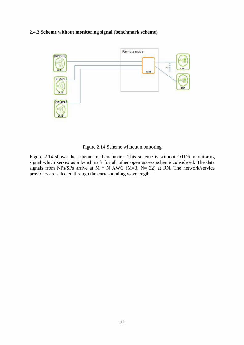
2.4.3 Scheme without monitoring signal (benchmark scheme)

Figure 2.14 Scheme without monitoring

Figure 2.14 shows the scheme for benchmark. This scheme is without OTDR monitoring

signal which serves as a benchmark for all other open access scheme considered. The data

signals from NPs/SPs arrive at M * N AWG (M=3, N= 32) at RN. The network/service

providers are selected through the corresponding wavelength.

13

Chapter 3. Measurements and Results

The various schemes discussed in Chapter 2 are implemented by using

VPItransmissionMaker 8.7. All NPs/SPs use the exactly the same set of wavelengths in the

tested open access WDM PON architecture. The wavelengths used for monitoring signals for

co-located FFs are also the same as in case with disjoint FFs connecting to different central

offices.

This chapter is organized as follows: introduction of VPItansmissionMaker in section 3.1.

Section 3.2 focuses on different modules that are used for simulation. Section 3.3 provides

information regarding methods for different schemes. Implementation of various schemes in

VPI is carried out in section 3.4 while the channel spacing impact is studied in section 3.5.

Section 3.6 provides the results of simulation and finally a discussion of the results is

included in section 3.7.

3.1 Introduction to VPItransmissionMaker

Figure 3.1 shows the various applications that can be designed using VPItransmissionMaker.

The development of hardware prototype will be difficult and costly. The best way is to model

the prototype in computer aided design with software simulation. It saves the cost as well as

time.

Figure 3.1 Applications of VPItransmissionMaker [15]

VPI photonics provides flexibility for various optical design problems by saving cost.

VPItransmissionMaker Optical Systems can fully verify link designs at a sampled-signal

level to identify further cost savings, investigate novel technologies, or fulfill specialist

requirements. Links can be automatically imported from VPIlinkConfigurator for detailed

design and optimization. VPItransmissionMaker is widely used as a research and

http://www.vpiphotonics.com/TMOpticalSystems.php

14

development (R&D) tool to evaluate novel component and subsystems designs in a systems

context, investigate and optimize systems technologies (e.g. coding, modulation, monitoring,

compensation, regeneration) for short-reach, access, aggregation, core and long-haul

applications. In addition to photonic transmission design suite (PTDS),

VPItransmissionMaker also offers VPIphotonicAnalyzer, VPIdesignRules, design assistant &

macros, simulation scripts, co-simulation capability, tailored user interface [15].

VPItransmissionMaker Optical Systems accelerates the design of new photonic systems

including short-range, access, metro and long haul optical transmission systems and allows

technology upgrade and component substitution strategies to be developed for existing

network plants. The combination of a powerful graphical interface, a sophisticated and robust

simulation scheduler together with flexible optical signal representations enables an efficient

modeling of any transmission system including bidirectional links, ring and mesh networks

[16].

3.2 Modules used in simulation

Optical Time Domain Reflectometer (OTDR)

OTDR is E-O device that detects and locates the fiber faults by determining the signals loss at

any point of the fiber. OTDR is used for construction, maintenance, fault location and

restoration of fiber. It is widely used to measure end to end loss, splicing loss, optical return

loss, locate the defects and breaks indicating optical alignment and detect the degradation of

fiber by making comparison with previous tests [17].

Figure 3.2 Block diagram of OTDR [18]

Figure 3.2 shows the block diagram of generic OTDR. The intensity of the laser diode is

modulated by the pulse generator which in turn is triggered by the signal processing unit. The

probe signal in OTDR is rectangular signal. To prevent the laser signal from saturating the

receiver, the source is coupled in a test fiber by directional coupler with sufficient isolation

magnitude between two ports. The directional coupler then guides the signal to the

photodetector. The photodetector can be PIN diode or APD which acts as a current source for

low noise amplifier thus providing linearity. Signals of several orders of magnitude are

incidents on photodiode thus receiver must have high dynamic range along with high

sensitivity. Analog to digital converter (ADC) forms interface to signal porcessing unit where

15

the data measured is processed and trace of fiber from the newtork monitored is computed.

The backscatter signal is normally weak so inorder to prevent it from covering of noise the

process of sending pulse and receiving must be repeated period of times to improve the SNR.

OTDR launches a short pulse into the fiber and measures the travelling time and the strength

of the reflected signal. Rayleigh scattering and Fresnel reflection cause the backscattering.

Figure 3.3 shows the trace of signal power vs distance.This represents the impulse response

of the link under the test. This trace provides information about link faults, fiber

misalignment, fiber mismatch, angular faults, dirt on connectors, macro bends and breaks.

These are referred to as events on OTDR trace. Fresnels reflection is caused due to mismatch

in refractive index which leasd to spikes in backscattered signal signifying the fiber end.

After the fiber end no signal is detected and the curve drops to receiver noise levels [19].

Figure 3.3 Sample of OTDR trace [19]

OTDR is implemented on VPItransmissionMaker to collect the backscatter signal in order to

localize and detect the faults. However the reflected signals in VPI are treated as distortions

and the information of their waveform is lost so the figure 3.2 cannot be implemented in

VPItransmissionMaker. Therefore a new design is required that neglects multiple reflections.

Figure 3.4 OTDR pulse generator

Figure 3.4 shows diagram of OTDR pulse generator implemented in VPItransmissionMaker.

Laser represents a distributed feedback (DFB) laser producing continuous optical signal.

16

Pseudo random binary sequence (PRBS) generates the binary sequence of 0s and 1s. The

pulse rectangular (electrical) generates sampled rectangular pulse for each input bit sequence

which is used to drive amplitude modulator (AM).Thus a rectangular pulse is generated by

co-work of PRBS, rectangular pulse and an AM. The transmitting power is 4 dBm and

wavelengths of L bands are used.

Optical Line Terminal (OLT)

OLT considered in the simulation consists of 32 channels with wavelength of C band and

transmitting power of 4 dBm. All NPs/SPs have same wavelength range. Unique PRBS is

used for each data channel in order to randomize the relative delay and phase between

transmitters. NRZ (Non Return Zero) coder generates NRZ coded signal by a sequence of

bits at its inputs which is produced by PRBS. Rise time adjustment transfer input electrical

pulses into smooth output pulse and is used to band-limit the modulated optical signal. Mach-

Zehnder modulator accepts a drive of 0 to 1 to give full extinction. The modulator with large

extinction and less chirp are desired because of pulse compression at 1.55µm.

OLT transmits the data signals with 32 channels, each of which has different wavelength. The

signals are multiplexed by the AWG and transmitted to the single mode fiber (SMF). The

schematic of OLT is different for co-located FFs and disjoint FFs as shown in figure 3.5 and

3.6 respectively.

Figure 3.5 OLT representations for co-located FFs in VPI

Figure 3.6 OLT representations for disjoint FFs in VPI

17

Arrayed Waveguide Grating (AWG)

WDM system supports large number of channels in a single fiber. In TDM PON optical

power splitter is used at RN. Downstream (DS) signals are sent to FF and then broadcasted

to multiple ONT by power splitter. In WDM PON, power splitter is replaced by AWG.

AWG works as multiplexer/demultiplexer (MUX/DEMUX), multiplexing at transmitting end

and demultiplexing at receiving end. They can be used to add/drop multiplexers, cross

connects and even used for routing.

Figure 3.7 Structure of arrayed waveguide grating (AWG) [20]

Figure 3.7 shows the structure of arrayed waveguide grating. The input consists of several

channels each carrying different frequency signals.The channel spacing of 100 GHz or 50

GHz are common in commercial available devices. The operating wavelength is around

1.55µm since the fiber attenuation is lowest at this wavelength. For propagation through the

device all AWG tend to be single moded.

Light from input waveguide couples into free propagaron range (FPR) and disperse to

arrayed waveguides (AW). Each AW exhibits a constant phase and path length increases for

each AW compared to previous array. The difference in path length ∆L is given by

∆L = m λ0/neff (3.1)

Where m is an integer, λ0 is the centre wavelength and neff is the refractive index of each

single mode waveguide [21]. At central wavelength constant phase profile is exhibited thus

lgiht focuses at centre of plane (e). Since different light has different amount of phase change,

the phase will change at AW output plane causing the focal point to move. An output

waveguide is positioned to pick each channel on output plane.

Figure 3.8 Schematic of N*N AWG with wavelength routing [22]

18

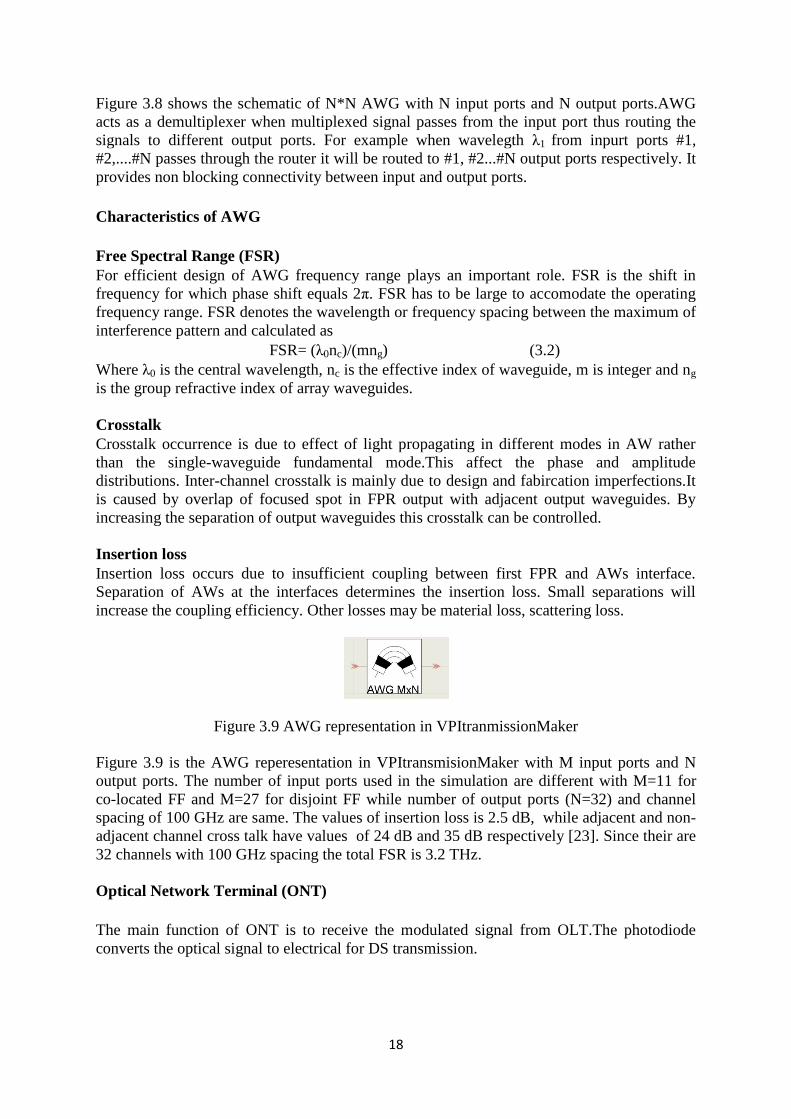
Figure 3.8 shows the schematic of N*N AWG with N input ports and N output ports.AWG

acts as a demultiplexer when multiplexed signal passes from the input port thus routing the

signals to different output ports. For example when wavelegth λ1 from inpurt ports #1,

#2,....#N passes through the router it will be routed to #1, #2...#N output ports respectively. It

provides non blocking connectivity between input and output ports.

Characteristics of AWG

Free Spectral Range (FSR)

For efficient design of AWG frequency range plays an important role. FSR is the shift in

frequency for which phase shift equals 2π. FSR has to be large to accomodate the operating

frequency range. FSR denotes the wavelength or frequency spacing between the maximum of

interference pattern and calculated as

FSR= (λ0nc)/(mng) (3.2)

Where λ0 is the central wavelength, nc is the effective index of waveguide, m is integer and ng

is the group refractive index of array waveguides.

Crosstalk

Crosstalk occurrence is due to effect of light propagating in different modes in AW rather

than the single-waveguide fundamental mode.This affect the phase and amplitude

distributions. Inter-channel crosstalk is mainly due to design and fabircation imperfections.It

is caused by overlap of focused spot in FPR output with adjacent output waveguides. By

increasing the separation of output waveguides this crosstalk can be controlled.

Insertion loss

Insertion loss occurs due to insufficient coupling between first FPR and AWs interface.

Separation of AWs at the interfaces determines the insertion loss. Small separations will

increase the coupling efficiency. Other losses may be material loss, scattering loss.

Figure 3.9 AWG representation in VPItranmissionMaker

Figure 3.9 is the AWG reperesentation in VPItransmisionMaker with M input ports and N

output ports. The number of input ports used in the simulation are different with M=11 for

co-located FF and M=27 for disjoint FF while number of output ports (N=32) and channel

spacing of 100 GHz are same. The values of insertion loss is 2.5 dB, while adjacent and non-

adjacent channel cross talk have values of 24 dB and 35 dB respectively [23]. Since their are

32 channels with 100 GHz spacing the total FSR is 3.2 THz.

Optical Network Terminal (ONT)

The main function of ONT is to receive the modulated signal from OLT.The photodiode

converts the optical signal to electrical for DS transmission.

19

Figure 3.10 Receiver for BER Estimation

Figure 3.10 shows the reciever with deterministic and stochastic BER estimation. It includes

polarization filter, photodetector, post detection LPF and clock recovery as shown in figure

3.11.

Figure 3.11 Internal structure of reciver module [24]

The photodetector can be either PIN diode or APD. In simulation PIN diode is used for

photodetetion. Sensitivity of PIN photodiode is given by (if only effect of thermal noise

included)[25]

S=QσT/R (3.3)

Where S is sensitivity (in Watts), Q is the desired Q factor (related to desired BER), R is

responsitivity of photodiode(A/W) and σT is the thermal noise current(A).

Thermal noise current σT is given by

σ2

T=STB (3.4)

where ST is the thermal noise spectral density (A2/Hz) and B is bandwidth of receiver (Hz).

To have a power budget of 20 dB (ITU-T recommendation G984.2 Class A), sensitivity of

receiver is -16 dBm since the transmitting power is 4 dBm. For the desired BER (at 10-9

) the

Q value is 6. The thermal noise spectral density value choosen for simulation is 10-22

A2/Hz.

Bandwidth is varied for the case with OTDR and without OTDR. So in order to have the

desired sensitivity the values of responsitivity is changed accordingly.

Fibers

The fiber model used in simulation is a simplified version of Universal fiber module for

simulation of a wideband nonlinear signal transmission in optical fiber with different

parameters for each fiber span individually. Figure 3.12 shows bidirectional fiber having two

input and output ports. The data signal is sent to forward input port and leaves the fiber

through forward output port. Since their is no any input to fiber in opposite direction it is

backscattered light.The length used for FF is 40 km and for DF is 5 km. The fiber attenuation

is 0.2 dB/km, dispersion is 16e-6 s/m2 and refractive index is 1.47.The non linear effects are

not considered since it doesnot have any effect for considered transmission power and

distance for FF and DF [23].

20

Figure 3.12 Scheme of a bidirectional fiber

Splitters

Splitters are used for broadcasting of signals. Two different splitters 1:8 and 3:8 is used in

simulation. In 1:8 splitter as shown in figure 3.13 the single signal is split into eight where as

in 3:8 as in figure 3.14, three signals comibine and then split into eight. To model the splitter

optical coupler is used. Optical coupler is used for combining or splitting of optical signals.

Figure 3.13 Scheme of 1:8 splitter

Figure 3.14 Scheme of 3:8 splitter

Optical switch

It provides the switching facility for signals in fiber from one circuit to another. It can work

physically by shifting fibers to drive other alternative fibers. In simulation 1:3 optical switch

is used. Figure 3.15 shows the scheme of 1:3 optical switch.

21

Figure 3.15 Scheme of 1:3 optical switch

Optical switch galaxy is implemeted in figure 3.16. The parameter PhaseShift determines the

behaviour of switch. If phaseshift is 0 degree the fisrt input will be routed to second output

and second input will be routed to first output. The change in behaviour will be inverse if the

phaseshift is chosen to be 180 degree[24].

Figure 3.16 Implementation of optical switch galaxy [24]

3.3 Methods

Four schemes are implemented in VPI and then compared with the benchmark case (without

monitoring signal). The schemes to be implented have two FFs layout, one co-located FFs

and another disjoint FFs. In co-located FFs three schemes are used: scheme with no filter,

scheme with one filter and scheme with three filters. In disjoint FFs, supervision scheme with

individual OTDR (vary in wavelength) in each CO are used.

The procedures while implementing these schemes are in order. Three NPs/SPs that are either

co-located in same CO or are in separate COs are used to transmit the data signal and OTDR

is used to transmit monitoring signal. Monitoring signal and data signal are separated at RN.

Data signal enters into input port of M*N AWG while monitoring signal passes through the

splitter and enters the other input ports of AWG. After AWG at RN the respected wavelength

is selected by again using the AWG. The signal is then sent to swept attenuator which

provides copies of input signal and the attenuation is increased for 20 steps starting from 0 dB.

A power meter provides the ROP where as receiver estimates BER. Receiver with

deterministic and stochastic BER estimation include polarization filter, PIN or APD

photodetector, post detection low pass filter and clock recovery. PIN photodetector is used as

receiver throughout the thesis. A plot of BER vs. ROP is created by sending measured power

to x-axis of NumericalAnalyzer2D and BER estimation to y-axis.

22

3.4 Implementation of schemes in VPI

The various open access supervision schemes discussed in chapter 2 are now implemented in

VPItransmissionMaker. Various methods are considered while implementing the schemes: no

channel spacing between NPs/SPs at AWG ingress port, channel spacing of four between

NPs/SPs and finally checking the impact of channel spacing for one of the schemes (three

filters case is taken). For each methods two cases are considered best case (only one NP/SP is

on and rests are off) and worst case (all NPs/SPs are on).

3.4.1 Open access scheme with no filter

Figure 3.1 Open access WDM-PON with no filter

Figure 3.17 shows the schematic modeled in VPItransmissionMaker for open access with no

filter. Here OTDR signal is not sent in any of the working FF but is sent by inserting an

additional FF. There is no need of filter either at CO and/or RN. Due to this there is no

additional loss introduced in any working path.

a) Best case with no channel spacing

Figure 3.18 Optical spectrum from first output port of RN AWG for no filter no channel

spacing best case

23

Figure 3.19 Eye diagram for no filter no channel spacing best case

b) Worst case with no channel spacing

Figure 3.20 Optical spectrum from first output port of RN AWG for no filter no channel

spacing worst case

Figure 3.21 Eye diagram for no filter no channel spacing worst case

c) Best case with four channel spacing

This case will be similar with best case for no channel spacing since only one NP/SP is

considered on. In simulation NP1/SP1 is on and remaining NPs/SPs are off.

24

d) Worst case with four channel spacing

Figure 3.22 Optical spectrum from first output port of RN AWG for no filter four channel

spacing worst case

Figure 3.23 Eye diagram for no filter four channel spacing worst case

3.4.2 Open access scheme with one filter

Figure 3.24 Open access WDM-PON with one filter

Figure 3.24 shows implementation of open access WDM-PON with one filter. Here the

monitoring signal is injected into FF of NP1/SP1. The signals combine into coupler which

has an insertion loss of 1 dB. The monitoring signals and data signals are separated at RN by

a filter. Filter also has an insertion loss of 1 dB. The data signal enters one port of AWG and

the monitoring signals passes through a 1:8 splitter which is then connected to other input

ports of AWG.

25


Figure 3.25 Optical spectrum from first output port of RN AWG for one filter no channel

spacing best case

Figure 3.26 Eye diagram for one filter no channel spacing best case

b) Worst Case with no channel spacing

Figure 3.27 Optical spectrum from first output port of RN AWG for one filter no channel

spacing worst case

26

Figure 3.28 Eye diagram for one filter no channel spacing worst case


It is similar with case a (best case for no channel spacing).


Figure 3.29 Optical spectrum from first output of RN AWG for one filter four channel

spacing worst case

Figure 3.30 Eye diagram for four channel spacing worst case

27

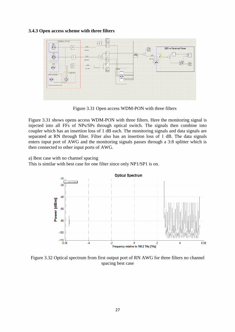
3.4.3 Open access scheme with three filters

Figure 3.31 Open access WDM-PON with three filters

Figure 3.31 shows opens access WDM-PON with three filters. Here the monitoring signal is

injected into all FFs of NPs/SPs through optical switch. The signals then combine into

coupler which has an insertion loss of 1 dB each. The monitoring signals and data signals are

separated at RN through filter. Filter also has an insertion loss of 1 dB. The data signals

enters input port of AWG and the monitoring signals passes through a 3:8 splitter which is

then connected to other input ports of AWG.


This is similar with best case for one filter since only NP1/SP1 is on.

Figure 3.32 Optical spectrum from first output port of RN AWG for three filters no channel

spacing best case

28

Figure 3.33 Eye diagram for three filters no channel spacing best case


Figure 3.34 Optical spectrum from first output of RN AWG for three filters no channel

spacing worst case

Figure 3.35 Eye diagram for three filters no channel spacing worst case


It is similar with case a (best case with no channel spacing).

29


Figure 3.36 Optical spectrum from first output port of RN AWG

for three filters four channel spacing worst case

Figure 3.37 Eye diagram for three filters four channel spacing worst case

3.4.4 Open access scheme with disjoint FFs layout

Figure 3.38 Open access WDM-PON with disjoint FFs

Figure 3.38 shows opens access WDM-PON with individual OTDR in each CO. Remote

node (RN) has same set of components for disjoint FF and CO however the wavelength for

each OTDR varies. The data and monitoring signal are first separated by filter for each

module. Filter has an insertion loss of 1 dB. The data signals enters input port of AWG and

30

the monitoring signals passes through a 1:8 splitter which is then connected to other input

ports of AWG.



for disjoint FFs no channel spacing best case

Figure 3.40 Eye diagram for disjoint FFs no channel spacing best case



for disjoint FFs no channel spacing worst case

31

Figure 3.42 Eye diagram for disjoint FFs no channel spacing worst case


This case is similar with best case with no channel spacing.



for disjoint FFs four channel spacing worst case

Figure 3.44 Eye diagram for four channel spacing worst case

32

3.4.5 Open access scheme with no monitoring signal (benchmark scheme)

Figure 3.45 Open access WDM-PON with no monitoring signal

Figure 3.45 shows open access WDM-PON with no monitoring signal. In this figure no

monitoring signal is applied, thus it acts as a benchmark for different schemes.


Figure 3.46 Optical spectrum from first output port of RN AWG for

benchmark no channel spacing best case

Figure 3.47 Eye diagram for benchmark no channel spacing best case

33


Figure 3.48 Optical spectrum from first output port of RN AWG for benchmark with no

channel spacing worst case

Figure 3.49 Eye diagram for benchmark with no channel spacing worst case

Figure 3.50 Open access WDM-PON for benchmark case with four channel spacing

34

Figure 3.50 shows open access WDM-PON schemes for benchmark case that has four

channel spacing. Spacing of four between the channels is done by grounding the ingress port

by using null source.


This case is similar with best case no channel spacing in case a.



for benchmark with four channel spacing worst case

Figure 3.52 Eye diagram for benchmark with four channel spacing worst case

3.5 Impact of channel spacing

In order to study how the performance of schemes varies when the interval of channel

spacing at AWG ingress port changes, different channel spacing is done at an ingress port of

AWG. For this, open access WDM-PON with three filters is taken into consideration with

channel spacing of one, two and four.

a) No channel spacing case

This case is same with the case a and b of section 3.4.3.

b) Channel spacing of one, two and four

From simulation it is found that the performance of the scheme improves by increasing the

channel spacing at ingress port of AWG compared with no channel spacing. The performance

remains same for all channel spacing except no channel spacing.

35

3.6 Results

The measurements are taken for different open access WDM-PON monitoring schemes.

Performance of four different schemes are measured and then compared with the benchmark

case which has no monitoring signal (i.e. no OTDR signal). In measurement, average value is

taken from five consecutive measurements by changing random number seed in PRBS in

order to get the stable values. Random number seed defines the seed value for the random

number generator. For all measurements, nine points are considered for measuring the

performance.

From the measured and calculated parameters, the values of different schemes are compared

with benchmark case to identify the power penalty. In all comparisons, plots with ROP in x-

axis and –log (BER) in y-axis are used.

Comparison of performance for no filter case

For this comparison, tables 1, 2 and 3 in appendix are referred.

Figure 3.53 Performance comparisons for the case with no filter

From the above plot it can be seen that there is power penalty of around 1 dB between best

case (blue line) and worst case (dark red line). With channel spacing of four between ingress

port the power penalty is reduced to 0.3 dB.

Comparison of Performance for one filter case

For this comparison, tables 4,5 and 6 in appendix are referred.

From the plot below it can be seen that the power penalty between the best case (blue line)

and worst case (dark red line) is around 1.7 dB. The power penalty improves to around 0.8

dB when there is spacing of four channels in between.

2 3 4 5 6 7 8 9

10 11 12 13 14 15 16 17 18 19 20

-27 -26.5 -26 -25.5 -25 -24.5 -24 -23.5 -23

-log(B

ER

)

ROP in dBm

Performance Comparison for No filter Case

Best case

Worst case

4 channel spacing worst case

36

Figure 3.54 Performance comparisons for the case with one filter

Comparison of Performance for three filters case

To compare this performance, tables 7, 8 and 9 in the appendix are referred.

Figure 3.55 Performance comparisons for the case with three filters

The best case for three filters is similar with best case for one filter because only NP1/SP1 is

turned on and others NPs/SPs are off. Moreover the insertion loss experienced is same so the

ROP is exactly the same as best case of one filter. But for worst case since all NPs/SPs are on

it will not be the same as the loss experienced differs. From the above plot the power penalty

for no channel spacing is around 0.8 dB (between blue line and dark red line). With the

spacing of four channels in between them now the performance improves. The power penalty

for this case is around 0.2 dB (between blue line and green line).

2 3 4 5 6 7 8 9

10 11 12 13 14 15 16 17 18 19 20

-27 -26.5 -26 -25.5 -25 -24.5 -24 -23.5 -23

-log(B

ER

)

ROP in dBm

Performance Comparison for One filter Case

best case

worst case

4 channel

spacing

worst case

2 3 4 5 6 7 8 9

10 11 12 13 14 15 16 17 18 19 20

-27 -26.5 -26 -25.5 -25 -24.5 -24 -23.5 -23

-lo

g(B

ER

)

ROP in dBm

Performance Comparison for Three Filters Case

Best case

Worst case

4 channel

spacing

worst case

37

Comparison of performance for disjoint FFs scheme

To compare for performance, tables 10, 11 and 12 in appendix are referred.

Figure 3.56 Performance comparisons for disjoint FFs

The best case of the above plot is almost similar to the best case of one filter and three filters

since they have exactly the same setup. Only the difference is in OTDR. In one filter and

three filter case OTDR is shared among all NPs/SPs where as in this case there is one

dedicated OTDR for each CO. From the above plot it can be found that the power penalty is

around 0.7 dB for no channel spacing case while it improves to about 0.1 dB for four channel

spacing when compared with best case.

Comparison of performance for benchmark case

For this comparison tables 13, 14 and 15 in appendix are referred.

Figure 3.57 Performance comparisons for the case with benchmark

This scheme does not have any monitoring signals so it is considered as a benchmark for

other schemes to compare. While measuring the performance of benchmark case itself there

is power penalty of around 1 dB with no spacing considered (blue line and dark red line).

Now with the spacing of four between the channels the power penalty is around 0.2 dB (blue

line and green line).

2 3 4 5 6 7 8 9

10 11 12 13 14 15 16 17 18 19 20

-27 -26.5 -26 -25.5 -25 -24.5 -24 -23.5 -23

-lo

g(B

ER

)

ROP in dBm

Performance Comparison for Disjoint Case

Best case

Worst case

4 channel

spacing

worst case

2 3 4 5 6 7 8 9

10 11 12 13 14 15 16 17 18 19 20

-27 -26.5 -26 -25.5 -25 -24.5 -24 -23.5 -23

-lo

g(B

ER

)

ROP in dBm

Performance Comparison for Benchmark Case

Best case

Worst

case

4 channel

spacing

worst case

38

Comparison of performance for all schemes with no channel spacing

In order to make this comparison, tables 1, 2, 4,5,7,8,10,11,13 and 14 in appendix are referred.

Figure 3.58 Performance comparisons of all schemes with no channel spacing

For comparison of best case, from the plot above it can be seen that benchmark and no filter

(dark blue line and green line) have almost same received power (penalty around 0.1 dB).

The plot for one filter best case (light blue line) and three filters best case is overlapped since

they have the same value of received power. The power penalty when compared with

benchmark is around 1.1 dB which is also for case with disjoint FFs (olive line). Now for

worst case comparison benchmark and no filter have penalty around 0.1 dB (dark red and

purple line). The power penalty for one filter, three filters and disjoint FFs in each CO are

around 1.8 dB, 0.9 dB and 0.8 dB respectively (dark red line, orange line, light pink line and

light purple line).

Comparison of performance for all schemes with four channel spacing

For this comparison tables 1, 3, 4, 6, 7, 9, 10, 12, 13 and 15 are referred in appendix.

The power penalties for best case with four channel spacing is same as that with the best case

for no channel spacing because of only one NP/SP on. However the power penalties for worst

case vary. The power penalties for worst case are compared with benchmark worst case (dark

red line). The power penalties for no filter (purple line), one filter (orange line), three filters

(light pink line) and disjoint FFs (light purple line) in each CO are around 0.1 dB, 1.7 dB, 0.9

and 0.9 dB respectively.

2 3 4 5 6 7 8 9

10 11 12 13 14 15 16 17 18 19 20

-27 -26.5 -26 -25.5 -25 -24.5 -24 -23.5 -23

-lo

g(B

ER

)

ROP in dBm

Performance for No Channel Spacing Benchmark

best case Benchmark

worst case No filter

best case No filter

worst case 1 filter best

case 1 filter worst

case 3 filters best

case 3 filters

worst case Disjoint best

case Disjoint

worst case

39

Figure 3.59 Performance comparisons of all schemes with four channel spacing

Comparison of performance for three filters with different channel spacing

For this comparison tables 7, 8 and 9 in appendix are referred. Other three tables are

discarded since they have same value as in table 9.

Figure 3.60 Performance comparisons for three filters with different channel spacing

2

3

4

5

6

7

8

9

10

11

12

13

14

15

16

17

18

19

20

-27 -26.5 -26 -25.5 -25 -24.5 -24 -23.5 -23

-lo

g(B

ER

)

ROP in dBm

Performance for 4 Channel Spacing Benchmark best case

Benchmark 4 channel spacing worst case

No filter best case

No filter 4 channel spacing worst case

1 filter best case

1 filter 4 channel spacing worst case

3 filters best case

3 filters 4 channel spacing worst case

Disjoint best case

Disjoint 4 channel spacing worst case

2 3 4 5 6 7 8 9

10 11 12 13 14 15 16 17 18 19 20

-27 -26.5 -26 -25.5 -25 -24.5 -24 -23.5 -23

-lo

g(B

ER

)

ROP in dBm

Impact of Channel Spacing for Three filters Best case

No channel spacing

1 channel spacing

2 channel spacing

4 channel spacing

40

To study the impact of channel spacing figure 3.60 is considered. With the increase in

channel spacing the power penalty is also improved. The power penalty improves from

around 0.8 dB (comparison between blue line and dark line) to 0.2 dB (comparison between

blue line and orange line). The orange line corresponds to channel spacing of four. Other

lines green and purple are overlapped with orange line since they have same values for

received power.

3.7 Discussion

From the results in the section 3.6 it is observed that for the best case, benchmark case and no

filter case have almost similar received power with power penalty of only about 0.1 dB. This

signifies there is negligible impact of monitoring signal on data signals. There is power

penalty of around 1.1 dB for one filter, three filters and disjoint FFs. This is mainly because

of the additional filter in scheme having an insertion loss of 1 dB.

Since all NPs/SPs (OLTs) are on in the worst case the BER performance decreases

significantly. It is because the crosstalk in AWG becomes dominant when all data signals are

transmitted by multiple OLTs. The power penalty for each schemes benchmark, no filter, one

filter, three filters and disjoint FFs when compared with their corresponding best case are 1.0

dB,1.0 dB, 1.7 dB, 0.8 dB, 0.7 dB respectively.

This performance degradation can be improved by increasing the channel spacing between

the ingress port of M*N AWG. When compared with their corresponding best cases the

power penalty are around 0.2 dB, 0.3 dB, 0.9 dB, 0.2 dB and 0.1 dB respectively for

benchmark, no filter, one filter, three filters and disjoint FFs. The improvement in BER

performance is because adjacent channel crosstalk will have less impact on data signals when

channel spacing is considered.

41

Chapter 4 Conclusion and Future Work

With the use of open access networks by operators and service providers its supervision is

extremely important. In this thesis various open access WDM-PON supervision schemes are

studied.

It has been found that multiple NPs/SPs can co-exist with wavelength selection. The

transmission performance analysis is carried out on VPI simulation. From the results it is

confirmed that there is no significant degradation on performance due to these schemes.

Moreover the monitoring signals have negligible impact on data signals. The worst

performance can further be improved by increasing interval between adjacent channels. All

the proposed schemes support fast monitoring.

Regarding the future work first it is necessary to solve the issues concerning the random

number seed for PRBS generator as its values keeps on changing. Second, since

implementation is based on some assumptions and simplified models, experimental

validation may be needed in future. Third, as this scheme is only for WDM-PON open access,

supervision schemes can be studied in various other types of PON. Fourth OFDR can be used

instead of OTDR for sending monitoring signals and checking whether it affects data signal

or not. Finally the cost associated with these monitoring schemes can be studied in future.

42

References

[1] C. H. Lee, W. V. Sorin and B. Y. Kim, “Fiber to the home using a PON infrastructure,” in

Journal of Lightwave Technology, vol. 24 issue 12, pp. 4568–4573, 2006.

[2] D. Gutierrez, W.T. Shaw, F.T. An, Y. L. Hsueh, M. Rogge, G. Wong, L. G. Kazovsky

and K.S. Kim,” Next Generation Optical Access Networks (Invited Paper),” in Broadband

Communications, Networks and Systems 2006.

[3] (2009) Frost & Sullivan Market Insight website. [Online]. Available: http://www.frost.com/prod/servlet/market-insight-print.pag?docid=184986442

[4] K. Yuksel, V. Moeyaert, M. Wuilpart and P. Megret, “Optical layer monitoring Passive

Optical Networks (PONs): A review,” in International Conference on Transport Optical

Networks 2008.

[5] P. J. Urban, “Drop-Link monitoring in Passive Optical Networks,” in International

Conference on Transport Optical Networks 2012.

[6] U. Hilbk, M. Burmeister, B. Hoen, T. Hermes, J. Saniter and F.J. Westphal, “Selective

OTDR measurements at the central office of individual fiber links in a PON,” in Optical

Fiber Communication 1997.

[7] P. J. Urban, G. Vall-llosera, E. Medeiros and S. Dahlfort, “Fiber Plant Manager: an

OTDR and OTM based PON monitoring system,” in IEEE Communications Magazine vol.51

issue 2, pp. S9-S15, 2013.

[8] M. Forzati, C.P. Larsen and C. Mattsson, “Open access networks, the Swedish

experience,” in International Conference on Transport Optical Networks 2010.

[9] (2012) Body of European Regulators for Electronics Communication website. [Online].

Available:

http://berec.europa.eu/eng/document_register/subject_matter/berec/reports/212-berec-report-

on-open-access

[10] (2011) International Telecommunication Union website. [Online]. Available:

http://www.itu.int/net/itunews/issues/2011/07/43.aspx

[11] J. Ikonen and M. Juutilainen, “User views on developing an open access network,” in

ChinaCom 2008, pp. 1355-1361, 2008.

[12] S. Verbrugge, K. Casier and C. M. Machuca, “Business models and their costs for next

generation access optical networks,” in International Conference on Transport Optical

Networks 2012.

[13] (2007) Zive website. [Online]. Available:

http://www.zive.sk/od-bpon-k-wdm-pon-hdtv-motivaciou/spravy/optika-do-domu-

technologie-pod-lupou/ch-182513-sc-30-a-273935/default.aspx

http://www.frost.com/prod/servlet/market-insight-print.pag?docid=184986442

http://www.itu.int/net/itunews/issues/2011/07/43.aspx

http://www.zive.sk/od-bpon-k-wdm-pon-hdtv-motivaciou/spravy/optika-do-domu-technologie-pod-lupou/ch-182513-sc-30-a-273935/default.aspx

http://www.zive.sk/od-bpon-k-wdm-pon-hdtv-motivaciou/spravy/optika-do-domu-technologie-pod-lupou/ch-182513-sc-30-a-273935/default.aspx

43

[14] W. V. Sorin, C-H. Lee and B. Y. Kim, “WDM-PON for FTTx,” A NIST symposium for

photonic and fiber measurements, pp. 98-103, 2006.

[15] VPITransmissionMaker Optical Systems User’s Manual.

[16] (2013) The VPIphotonics website. [Online].Available:


[17] (2000) Celemetrix website. Available:

http://www.celemetrix.com.au/document/item/1011 ”Understanding OTDRS”

[18] J. Beller, “OTDRs and backscatter measurements,” in Fiber Optic Test and

Measurement, Chapter 11, pp. 434-474, 1998.

[19] M. M. Rad, K. Fouli, H. A. Fathallah, L. A. Rusch, M. Maier, “Passive optical network

monitoring: challenges and requirements,” IEEE Communications Magazine, vol. 49 issue 2,

pp s45-s52, 2011.

[20] K. A. McGreer, “Arrayed waveguide gratings for wavelength routing”, IEEE

Communications Magazine, vol. 36 issue 12, pp. 62-68, 1998.

[21] P. Munoz, D. Pastor, and J. Capmany, “Modeling and design of arrayed waveguide

gratings,” Journal of Lightwave Technology, vol. 20 issue 4, pp. 661-674, 2002.

[22] S. Kamei, M. Ishii, A. Kaneko, T. Shibata and M. Itoh, “NxN cyclic-frequency router

with improved performance based on Arrayed-Waveguide Grating,” Journal of Lightwave

Technology, vol. 27 issue 18, pp. 4097–4104, 2009.

[23] J. Chen, L. Wosinka, M. N. Chughati and M. Forzati, “Scalable passive optical network

architecture for reliable service delivery,” IEEE/OSA Journal of Optical Communication and

Networking, vol.3 issue 9, pp.667-673, 2011.

[24] VPItransmissionMaker Module Reference.

[25] Optiwave (Design software for photonics) website. Available:

http://www.optiwave.com/academia/labs/lesson6/Receiver_Sensitivity.pdf


http://www.celemetrix.com.au/document/item/1011

http://www.optiwave.com/academia/labs/lesson6/Receiver_Sensitivity.pdf

44

Appendix

Appendix 1: List of simulation parameters

Segment Device Parameter Value

Global parameters Time Window 128/Bit Rate Default

s

Sample Mode

Bandwidth

1280 * Bit Rate

Default Hz

Sample Mode Center

Frequency

192.8e12 Hz

Sample Rate Default 64 * Bit Rate Default

Hz

Bit Rate Default 1e9 bits/s

OTDR Pulse

Genererator

CW laser (for co-

located FFs/CO1

disjoint FF)

Emission Frequency 184.5e12 Hz

Sample Rate Sample Rate Default

Hz

Average Power 2.51e-3 W

Linewidth 10e6 Hz

CW laser for CO2 Emission Frequency 184.6e 12 Hz

CW laser for CO3 Emission Frequency 184.7 e 12 Hz

Pseudo Random

Binary Sequence

(PRBS) Generator

Bit rate Bit Rate Default

bits/s

PRBS_Type PRBS

Mark Probability 0.5

Pulse Rectangular

(Electrical)

Bit Rate Bit Rate Default

bits/s

Amplitude

Modulator


Hz

Pulse Length Ratio 1.0

Amplitude 1.0

Modulation Index 1.0

Data signal source CW-Laser 1 Emission Frequency 192.8 e12 Hz


Hz

Average Power 2.51e-3 W

Linewidth 10e6 Hz

PRBS Generator

1~PRBS Generator

32

Bit Rate Bit Rate Default

bits/s

PRBS_Type PRBS

Mark Probability 0.5

NRZ1~NRZ32 Bit Rate Bit Rate Default

bits/s


Hz

Rise time

adjustment1~Rise

time adjustment 32

Rise Time 1.0/4.0/Bit Rate

Default s

Mach Zehnder Extinction 30.0 dB

45

1~Mach Zehnder 32 Chirp Definition Symmetry Factor

Symmetry Factor 0.5

Chirp Design Positive

Channel Index -1

CW-Laser 2 Emission Frequency 192.9 e12 Hz

CW-Laser 3 Emission Frequency 193.0e12 Hz

























CW-Laser 28 Emission Frequency 195.5 e12 Hz





CW-Laser 1~CW-

Laser32

Sample Rates, Average Powers, Linewidths

are same

Fiber Feeder Fiber

1~Feeder Fiber 4

Number of Fiber

Spans

1

Length 40e3 m

Group refractive

index

1.47

Attenuation 0.2e-3 dB/m

Dispersion 16e-6 s/m2

Dispersion slope 0.08e-3 s/m3

Raman Scattering No

Higher Order NL

effects

No

46

Polarization Analysis Yes

Field Analysis Yes

Event Loss 0.0 dB

Drop Fiber Length 5e3 m

Remaining parameters are same as that of FF

Coupler WDM-Mux

N_1_Ideal

Insertion loss 1.0 dB

Optical Filter Data Filter1~Data

Filter 3

Filter type Band Pass

Transfer Function Gaussian

Bandwidth 3.3e12 Hz

Center frequency 194.4e12 Hz

Gaussian order 1

Noise Resolution Bit Rate Default/4

Hz

Active Filter

Bandwidth Center

Frequency

194.4e12 Hz

Monitoring signal

filter(for co-located

FF and CO1 for

disjoint FF)

Bandwidth 4* Bit Rate Default

Hz


Active Filter

Bandwidth Center

Frequency

184.5e12 Hz

Monitoring signal

filter for CO2 of

disjoint FF


Hz


Active Filter

Bandwidth Center

Frequency

184.6e12 Hz

Monitoring signal

filter for CO2 of

disjoint FF


Hz


Active Filter

Bandwidth Center

Frequency

184.7e12 Hz

1:8Splitters/ 3:8

Splitter

X Coupler Couple Factor 0.5

1:3 Optical Switch Optical Switch Phase Shift 0.0 deg

Couple Factor1 0.5

Couple Factor 2 0.5

Array Waveguide

Grating

32 * 1 AWG Number of Input

Ports

32

Number of Output

Ports

1

Operating Frequency

range

180e12~250e12 Hz

Channel Frequency 192.8e12 Hz

Channel Spacing

Output

-100.0e9 Hz

47

Colorless On

Free Spectral Range 3.2e12 Hz

Model Type Datasheet

Passband Type Gaussian

Bandwidth_3 dB 55.0e9 Hz

Dispersion Mininum -1.0e-2 s/m

Dispersion

Maximum

16.0e-6 s/m

Adjacent Crosstalk 24.0 dB

Non Adjacent

Crosstalk

35.0 dB

Insertion Loss 2.5 dB

Noise Resolution Bit Rate Default/4

M * N AWG

M=11 & N=32 (co-

located FFs)

M=27 & N=32

(disjoint FFs)

Number of Input

ports

11 or 32

Number of Output

ports

32

Remaining all the values are same as that of

31 * 1 AWG

Swept Attenuator Lowest Attenuaation 0 dB

Increment 1 dB

Number of Steps 20

Power Meter Limit Bandwidth Off

Include Sampled

Signals

On

Include Noise Bins On

Meas Mode Total

Output Units dBm

Receiver with

Deterministic and

Stochastic BER

Estimation

Detector Resample Rate Sample Rate Default

Detector Type PIN

Dark Current 0 A

Include Shot Noise Yes

Thermal Noise 10.0e-12 A/√Hz

Post Detection Filter Electrical LP Filter

Type

Bessel

Bandwidth 0.75 * Bit Rate

Default Hz

Filter Order 3

Bilinear Transform On

BER Estimator Optical Noise

Treatment

Stochastic

BER_Required 1.0 e-9

Estimation Method

Stochastic

Gauss_ISI

Sample Type Optimum

Threshold Type Optimum

Outputs BER

48

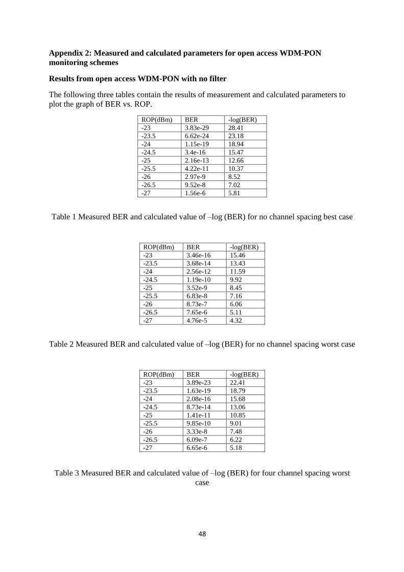
Appendix 2: Measured and calculated parameters for open access WDM-PON

monitoring schemes

Results from open access WDM-PON with no filter

The following three tables contain the results of measurement and calculated parameters to

plot the graph of BER vs. ROP.

ROP(dBm) BER -log(BER)

-23 3.83e-29 28.41

-23.5 6.62e-24 23.18

-24 1.15e-19 18.94

-24.5 3.4e-16 15.47

-25 2.16e-13 12.66

-25.5 4.22e-11 10.37

-26 2.97e-9 8.52

-26.5 9.52e-8 7.02

-27 1.56e-6 5.81

Table 1 Measured BER and calculated value of –log (BER) for no channel spacing best case


-23 3.46e-16 15.46

-23.5 3.68e-14 13.43

-24 2.56e-12 11.59

-24.5 1.19e-10 9.92

-25 3.52e-9 8.45

-25.5 6.83e-8 7.16

-26 8.73e-7 6.06

-26.5 7.65e-6 5.11

-27 4.76e-5 4.32

Table 2 Measured BER and calculated value of –log (BER) for no channel spacing worst case


-23 3.89e-23 22.41

-23.5 1.63e-19 18.79

-24 2.08e-16 15.68

-24.5 8.73e-14 13.06

-25 1.41e-11 10.85

-25.5 9.85e-10 9.01

-26 3.33e-8 7.48

-26.5 6.09e-7 6.22

-27 6.65e-6 5.18

Table 3 Measured BER and calculated value of –log (BER) for four channel spacing worst

case

49

Results from open access WDM-PON with one filter




-23 2.72e-19 18.56

-23.5 6.76e-16 15.17

-24 3.87e-13 12.41

-24.5 6.69e-11 10.17

-25 4.36e-9 8.36

-25.5 1.28e-7 6.89

-26 2.00e-6 5.70

-26.5 1.85e-5 4.73

-27 1.12e-4 3.95



-23 5.13e-10 9.28

-23.5 6.19e-9 8.20

-24 5.68e-8 7.24

-24.5 5.34e-7 6.27

-25 3.69e-6 5.43

-25.5 2.3e-5 4.64

-26 1.06e-4 3.97

-26.5 4.11e-4 3.39

-27 0.0012 2.92



-23 1.04e-13 12.98

-23.5 1.74e-11 10.76

-24 1.15e-9 8.94

-24.5 3.93e-8 7.40

-25 6.96e-7 6.16

-25.5 7.49e-6 5.12

-26 5.16e-5 4.29

-26.5 2.52e-4 3.60

-27 9.18e-4 3.04


case

50

Results from open access WDM-PON with three filters




-23 2.72e-19 18.56

-23.5 6.76e-16 15.17

-24 3.87e-13 12.41

-24.5 6.69e-11 10.17

-25 4.36e-9 8.36

-25.5 1.28e-7 6.89

-26 2.00e-6 5.70

-26.5 1.85e-5 4.73

-27 1.12e-4 3.95



-23 1.56e-12 11.81

-23.5 4.12e-11 10.38

-24 7.23e-10 9.14

-24.5 1.29e-8 7.89

-25 1.53e-7 6.81

-25.5 1.58e-6 5.80

-26 1.11e-5 4.95

-26.5 6.30e-5 4.20

-27 2.64e-4 3.58



-23 3.97e-17 16.40

-23.5 2.60e-14 13.6

-24 4.78e-12 11.32

-24.5 4.21e-10 9.37

-25 1.65e-8 7.78

-25.5 3.47e-7 6.45

-26 4.16e-6 5.38

-26.5 3.22e-5 4.49

-27 1.7e-4 3.77


case

51

Results from open access WDM-PON with disjoint FFs




-23 1.00e-19 19

-23.5 2.98e-16 15.52

-24 1.99e-13 12.70

-24.5 3.89e-11 10.41

-25 2.82e-9 8.55

-25.5 9.02e-8 7.04

-26 1.50e-6 5.82

-26.5 1.46e-5 4.83

-27 9.3e-5 4.03



-23 4.51e-13 12.34

-23.5 1.45e-11 10.84

-24 3.56e-10 9.45

-24.5 6.68e-9 8.17

-25 9.08e-8 7.04

-25.5 9.41e-7 6.03

-26 7.24e-6 5.14

-26.5 4.24e-5 4.37

-27 1.91e-4 3.72

Table 11 Measured BER and calculated value of –log (BER) for no channel spacing worst

case


-23 1.02e-17 16.99

-23.5 6.00e-15 14.22

-24 1.40e-12 11.85

-24.5 1.38e-10 9.86

-25 6.51e-9 8.18

-25.5 1.57e-7 6.80

-26 2.18e-6 5.66

-26.5 1.87e-5 4.73

-27 1.09e-4 3.96


case

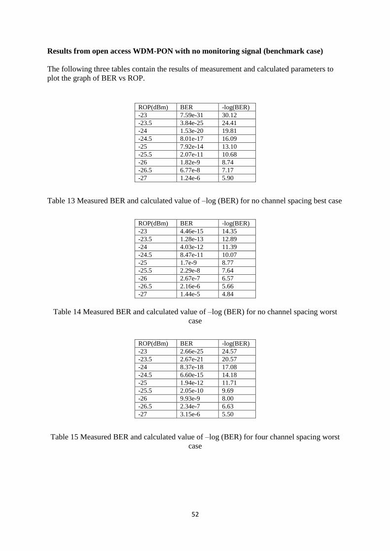
52

Results from open access WDM-PON with no monitoring signal (benchmark case)


plot the graph of BER vs ROP.


-23 7.59e-31 30.12

-23.5 3.84e-25 24.41

-24 1.53e-20 19.81

-24.5 8.01e-17 16.09

-25 7.92e-14 13.10

-25.5 2.07e-11 10.68

-26 1.82e-9 8.74

-26.5 6.77e-8 7.17

-27 1.24e-6 5.90



-23 4.46e-15 14.35

-23.5 1.28e-13 12.89

-24 4.03e-12 11.39

-24.5 8.47e-11 10.07

-25 1.7e-9 8.77

-25.5 2.29e-8 7.64

-26 2.67e-7 6.57

-26.5 2.16e-6 5.66

-27 1.44e-5 4.84

Table 14 Measured BER and calculated value of –log (BER) for no channel spacing worst

case


-23 2.66e-25 24.57

-23.5 2.67e-21 20.57

-24 8.37e-18 17.08

-24.5 6.60e-15 14.18

-25 1.94e-12 11.71

-25.5 2.05e-10 9.69

-26 9.93e-9 8.00

-26.5 2.34e-7 6.63

-27 3.15e-6 5.50


case

www.kth.se


Study on Fault Detection and Localization for Wavelength ... · Wavelength division multiplexing...

Documents

Transcript of Study on Fault Detection and Localization for Wavelength ... · Wavelength division multiplexing...