Università della Svizzera Italiana (University of Lugano)

Faculty of Economics

Institute of Management

STUDY ON BEHAVIORAL PATTERNS IN

QUEUING: AGENT BASED MODELING AND

EXPERIMENTAL APPROACH

KARTHIK SANKARANARAYANAN

Supervisors

Prof. Erik R. Larsen

Prof. Ann van Ackere

Thesis submitted in partial fulfilment of the requirements for the degree of Doctor of

Philosophy in management at The Università della Svizzera Italiana (University Of Lugano),

October 2011.

Imagination is more important than knowledge, for knowledge is limited

while imagination embraces the entire world.

Albert Einstein

ABSTRACT

“Time is money” if you are a service provider or a customer using the service. In the current economic

scenario where there is heavy competition, customers have more alternatives at their disposal; which

means understanding customers is of paramount importance. This dissertation delves into this terrain,

and tries to provide a conceptual and an experimental framework to understand the complex dynamics

we see every day in queuing.

The traditional approach to queuing has been towards designing an efficient facility, with little focus

towards the customers who use these facilities. This approach has been helpful to understand the

capacity requirements, and the impact of different configurations of production and service facilities,

but has limited our ability to explain the behavior observed in many real queues. This dissertation

continues the shift in focus from the service facility design to the information structure, and the

behavior of the customers in a queuing system. Two extensions are proposed to the traditional queuing

framework: Customers are provided with 1) information regarding the performance of the facility

(feedback) and 2) computational capability to process the information provided. In a nutshell, the

customers in this model choose which facility to use depending on their expectations which are based

on past experiences.

I present two agent based modeling frameworks to characterize the customers using the facility. This

approach helps us to model homogenous customers, and it is useful because every customer perceives

differently the cost of waiting and also the efficiency of the system. Agent based models help to

understand how the customers might co-evolve with the facility that serves them, which is difficult to

achieve within the traditional queuing framework. Finally, an experiment is designed using the

guidelines from experimental economics to validate the agent based modeling framework.

Key words: Behavioral queuing, agent based modeling, experimental economics.

ACKNOWLEDGEMENT

“Matha, Pitha, Guru, Deivam” is a very popular adage used in Sanskrit language. Literally translated it

is “Mother, Father, Teacher and God”. It tells about the order in which a human being should pay

respect. So going with this adage, I would like to first pay my heartfelt gratitude to my parents

Rajeswary and Sankarnarayanan for being there, supporting me at every nook and corner of life, not

just for this work, but since those baby steps. I know saying thanks will not even remotely express how

grateful I am to them, nevertheless, thanks a ton mama and papaji. The next person in my family to

whom am heavily indebted is my sister Kavitha, my mentor, friend, advisor, partner in mischief etc. SK

your motivation and unflinching confidence in me helped me reach where I am today. Also thanks to

my brother-in-law Jayan. J you have been more of a friend and brother, thanks for extending a helping

hand whenever needed. Then an important person in our family, my nephew Srivats, cheechu thanks

for all the fun and entertainment during the past 3 years. Finally, last but not least to the new person in

our family, my fiancé Vanishree. She has patiently listened to my blabbering, supported me, and in

spite of the physical distance has been close enough to share my last few years in Switzerland. Thanks

for your love. I am also grateful to my in laws Anna and Amma for their patience and support.

After parents, it is the teachers who help hone a person. My sincere thanks and gratitude to Professor

Erik Larsen and Professor Ann van Ackere. It was a real honour to work under their supervision.

Thanks for the confidence you placed in me and also the opportunities that you created for me to learn

and develop myself. Prof. Larsen you are the coolest supervisor a student can have. Thanks for giving

me this opportunity, listening to me patiently, advising me whether it is research or something personal

and most importantly supporting me all the time. Prof. van Ackere thanks for accommodating me at

UNIL every time I was there, patiently looking at my articles, pushing me hard to make my papers

better and helping me out for the last four years. Finally, I would also like to thank all the faculty

members at the Institute of Management, USI for their support and guidance.

I have made a lot of friends during the last 7 years in Switzerland; it was an amazing journey and would

like to thank all of them for making it memorable. I would like to thank my friends at IMA Jaime,

Chanchal, Mohammad, Marco, Pooya, Min, Margarita, Lei, Cecile, Guido, Fabi and the other post-

docs for their support. A special thanks to Soorjith and Sayed (my flatmates, friends and also

colleagues at IMA) for their support and the late night discussions on movies, politics etc. Thanks to

Carlos, Crina and Camila at UNIL and Santiago from Colombia for their help. Special thanks to

Sabrina (USI) for the long discussions about research, life in general, business ideas and most

importantly being a good friend.

I would like to thank Abraham uncleji, Anniamma auntyji, Manoj and Manju for accommodating me

in their house, treating me as a family member, for the Indian food and also for the awesome time we

had while travelling around Switzerland and Europe. Thanks to Antoneyji, Miniji, Kiran and Arun for

their support. Antoneyji and Miniji thanks for your support, and the trust you placed in me. Finally my

philosophical, kind and always helpful Italian (99% Indian even though her passport says she is Italian)

friend Anna Pischetta. Anna you have been of tremendous support, thanks for listening to me, and

most importantly being a good friend.

Finally, thanks to the Swiss National Science Foundation for funding my doctoral studies. Thanks to

all the administrative and support staff at USI who have helped me and thanks to all the people whom

I might have forgotten to mention.

TABLE OF CONTENTS

1. Introduction ……………………………………………………………………….. 1

2. Queuing …………………………………………………………………………… 5

3. Research methodologies

3.1 Agent based modelling ………………………………………………………….. 13

3.2 Evolutionary computation & genetic algorithms …………………………………. 17

3.3 Experimental methods ………………………………………………………….. 22

4. Papers

4.1 The micro-dynamics of queuing: Understanding the formation of queues ………… 27

4.2 Modelling decision making in an adaptive agent based queuing system using cellular automata

and genetic algorithms . …………………………………………………………….. 46

4.3 A tale of three restaurants: An experimental approach to understand decision making in

queuing systems. ……………………………………………………………………. 63

5. Conclusion. ………………………………………………………………………… 106

6. Bibliography………………………………………………………………………… 111

LIST OF FIGURES

Figure 2.1 A simple queuing system

Figure 3.1 Agent

Figure 3.2 Steps in an experimental method

Figure 4.1 The spatial-temporal evolution of the choice of service facility over fifty periods. Each

color represents a facility (Black = facility 1, Grey = facility 2, White = facility 3)

Figure 4.2a Shows the average sojourn time as well as the minimum and maximum experienced by

any of the 120 agents in a given time period

Figure 4.2b Shows the minimum and maximum sojourn time experienced by any of the agents (i)

over the full 50 periods (ii) for the steady state period of 25-50

Figure 4.3a The realized sojourn time and the expectation (memory) of agent 20

Figure 4.3b Facility frequented by agent 20

Figure 4.4 A spatial-temporal simulation with the same parameters as was used in figure 1 but

with a different set of initial conditions, developing a different pattern of choices,

ending up “forgetting” one of the facilities

Figure 4.5 The distribution of average travel time for 1000 simulation with different initial

conditions for α and β = 0.5

Figure 4.6 The average sojourn time as a function of α for selected values of β. Each recorded

values of α represents the average of 1000 simulations with different initial values.

Note that for reasons of legibility the Y-axis starts at 1.5

Figure 4.7 Results for different values of α and β. In (a) and (b) α=β=0.1 while in (c) and (d)

α=β=0.9

Figure 4.8 Results from a run where α and β are allocated randomly to each agent

Figure 4.9 GA flowchart

Figure 4.10 Population average of all CA’s (average sojourn time) for each generation

Figure 4.11(a) First generation CA’s average sojourn time

Figure 4.11(b) Last generation CA’s average sojourn time

Figure 4.12 Population average of all CA’s (average sojourn time) for each generation

Figure 4.13.a Population average over generations while varying the mutation rate for homogenous

service rate

Figure 4.13.b Population average over generations while varying the mutation rate for heterogeneous

service rate

Figure 4.14 Structure of cellular automata agent based queuing model

Figure 4.15 Evolution of agents’ choice of service facility for homogenous (a, b, c) and

heterogeneous (d, e, f) service rates

Figure 4.16 Average sojourn time with minimum and maximum value

Figure 4.17 Evolution of players choice of service facility for homogenous (a, b, c) and

heterogeneous (d, e, f) service rates

Figure 4.18 Individual decision making for group E treatments virtual agent (a, b, c) vs human

subject (d, e,f)

Figure 4.19 Individual decision making for group D treatments virtual agent (a, b, c) vs human

subject (d, e,f)

Figure 4.20 Experimental (Exp) and simulated (Sim) average sojourn time in steady state

comparison for group E treatments

Figure 4.21 Experimental (Exp) and simulated (Sim) average sojourn time in steady state

comparison for group D treatments

Figure 4.22 Box plot for the average sojourn time in steady state of subjects for group E treatments

Figure 4.23 Box plot for the average sojourn time in steady state of subjects for group D treatments

LIST OF TABLES

Table 2.1 Literature overview (adapted from van Ackere and Larsen, 2007)

Table 4.1 Parameter values used for the base case as well as the range used for experiments.

Table 4.2 Parameter values used for the base case

Table 4.3 GA parameter notations

Table 4.4 Varying the mutation rate for homogenous service rates

Table 4.5 Varying the mutation rate for heterogeneous service rates

Table 4.6 Varying the selection rate

Table 4.7 Varying the population size

Table 4.8 Treatment conditions for homogenous service capacities

Table 4.9 Treatment conditions for heterogeneous service capacities

Table 4.10 Behavioral parameter values interpretations

Table 4.11 Notations for variables in tables 4.12 and 4.13

Table 4.12 Human subjects and the observed behavioral patterns for group E treatments

Table 4.13 Human subjects and the observed behavioral patterns for group D treatments

Table 4.14 Notations for variables in figures 4.20 and 4.21

Table 4.15 P-values of Wilcoxon Rank-Sum test for the average sojourn time in steady state of

subjects for group E treatments

Table 4.16 P-values of Wilcoxon Rank-Sum test for the average sojourn time in steady state of

subjects for group D treatments

Table 4.17 Collection of strategies that could be used to choose a restaurant

Table 4.18 Matching strategies with that of human subjects’ strategies

Table 4.19 Human subjects’ distribution across various alpha and beta values for strategies S27

and S28 among group treatments

Table 4.20 Contribution to literature

1. INTRODUCTION

Queuing theory is a widely studied branch in operations research and is used to make important

decisions regarding the allocation of resources. Queuing is a way of life and we experience it every day.

The systematic study of queuing dates back to 1909 when Erlang (1909), a Danish engineer, published

the first paper on queuing theory applied to traffic in telephone networks. He is considered to be the

pioneer of queuing theory and since then it has been researched extensively and its application spans

telecommunications, healthcare, traffic, and computer networks to name a few.

Most of the research in the area of queuing since Erlang has focused predominantly on designing

efficient systems. Most of the queuing models assume static conditions with exogenous arrival and

service rates and are analysed in steady-state. The impact of individual decision making on queuing (i.e.

how individual expectation formation affects queuing) and selection of service facility based on

experience has been largely neglected.

The seminal papers addressing the behaviour of agents involved in a queuing system are that of Naor

(1969) and Yechiali (1971). In his 1969 paper, Naor focused on decision processes in queuing which

was a shift from the design centric approach to queuing. Yechiali (1971) extended Naors’ work; both

adopt an analytical approach and propose the use of tolls to control queue size. Since then Stidham

(1985), Dewan and Medelson (1990), van Ackere (1995), Rump (1998), Zohar et al. (2002),

Haxholdt et al. (2003) and van Ackere et al. (2006) have explored this idea. Koole and Mandelbaum

(2002) raise the issue of the need to include behavioural factors in telephone call centre queuing

models and call it a complex socio-technical system. Hassin and Haviv (2003) provide a

comprehensive survey of equilibrium behaviour of customers and servers in queuing systems. van

Ackere and Larsen (2004) analyze customers’ choice based on feedback and how they form

expectations based on local information and their experiences in the system.

1

There has also been a trend towards understanding the behavioural aspects in complex decision

problems named behavioural operations (Gino and Pisano, 2008; Loch and Wu, 2008). This research

area has used experiments and covers supply chains, commodity research (Sonnemans et al., 2004;

Sterman, 1989) and to some extent queuing (Rapoport et al., 2010; Rapoport et al., 2004; Stein et al.,

2007).

This thesis builds on the work of van Ackere and Larsen (2004) and seeks to understand customers’

behaviour in a multi-channel service facility. The idea is to understand decision making and the effects

of local information and adaptive expectations on the decision making process. The dissertation thus

looks into interactions among customers within a system and how it influences the systems’

performance, which in turn affects customers’ perception of the system. We are all aware of the famous

adage “Time is money” and this applies to a service provider and to customers who use the service. In

the current economic scenario where there is heavy competition, customers have more alternatives at

their disposal, which means that understanding customers' needs is of paramount importance. This

thesis delves into this terrain and tries to provide both a theoretical and an experimental framework to

understand the complex dynamic behaviour that we observe every day in queuing.

The motivation for this doctoral dissertation thus stems from the fact that queuing research has looked

towards the use of analytical tools to solve system design issues and neglected the behaviour of

customers to a large extent. These analytical models in order to arrive at a closed form solution

sometimes make unrealistic assumptions leading to suboptimal design; hence simulation is used as a

methodology to study behaviour in queues. Agent based modelling and simulation (North and Macal,

2007) is a natural choice to model such a system.

The thesis implements this self-organizing (van Ackere and Larsen, 2004) agent based modelling

framework by using cellular automata and captures the nonlinear interactions of customers (the term

customer represents both living and non-living items; hence the term “agent” will be used henceforth).

2

In the dissertation we propose two frameworks : 1) the first is based on cellular automata (CA)

(Gutowitz, 1991; Wolfram, 2002) and adds an extension to it by providing a memory structure. This

helps to model the behaviour of individual agents and study how they evolve based on their

experiences. 2) The second framework uses genetic algorithms (GA) (Goldberg, 2009; Haupt and

Haupt, 2004b; Mitchell, 2001) to model adaptive agents or intelligent agents. In this way by finding

the best combination of behavioural parameters for the CA, the overall system is optimized. Thus the

thesis looks at both the individual level and the system as a whole.

Finally an experimental approach (Friedman and Sunder, 1994; Guala, 2008; Smith, 1982; Smith,

1989) is adopted as a methodology to validate the findings of the agent based framework. The idea is

to collect data from human subjects who will take up the role of one of the virtual agents. This

approach aims to validate the simulated results and see if human subjects’ decision making follows the

same characteristics as proposed in the agent based framework.

The thesis is structured as follows: Chapter 2 presents a literature review on queuing; Chapter 3 gives a

brief description of the research methodologies and methodological ideas that are adopted in this

thesis; Chapter 4 presents the research contributions of this thesis in the form of scholarly papers. The

format of the thesis is cumulative, i.e., it integrates three individual papers into one. Section 4.1 in

chapter 4 introduces the agent based behavioural queuing framework. Using cellular automata a self-

organizing behavioural queuing system is built. The idea behind this paper is to investigate the micro

foundation of queuing and macro effects for the system. The paper shows how, using adaptive

expectations based decision rules, different collective behaviours can be observed.

Section 4.2 presents another agent based framework based on genetic algorithms. This model takes the

CA model a step further by modelling how customers evolve, and how they optimize their behaviour as

they experience the consequence of queuing. Using genetic algorithms, this paper optimizes the

behavioural parameters of the behavioural queuing model of section 4.1.

3

In section 4.3, an experimental approach is proposed to validate the behavioural queuing model

described in section 4.1. The aim of this paper is to understand the influence of human subjects on the

performance of the system. By using various treatments, the paper investigates the influence of

structural and behavioural properties on human subjects’ decision making. The influence of

information and the perception of the same are also studied. Finally, chapter 5 summarizes and

concludes the thesis by pointing out its contributions and avenues for future work.

4

CHAPTER 2: QUEUING

2.1 Introduction

“Queue” is a word that every human being on earth would have heard and “queuing” is a phenomenon

that is being experienced on a daily basis. We stand or wait in queues at supermarkets, airports,

restaurants, post offices or virtually queue at our desks when we are on hold at a call center. Do people

like to wait? The answer is of course “NO”. Do managers or businesses like customers waiting? The

answer again is no because they may lose customers as well as receive a bad reputation. Why then are

there queues and why do we have to wait? One reason that comes to mind immediately is that there is

more demand than available service capacity. Why not add more capacity? Adding capacity might not

be feasible either economically or due to space limitations. Hence this warrants the development of a

scientific method of optimally designing a facility keeping in mind the economics as well as the quality

of service.

Queuing theory (Gross and Harris, 1998), defined as the mathematical study of queues, helps us to

overcome these limitations by trying to answer questions like:

1) The number of required service facilities to cater to the needs of the customers.

5

Arrival

Server/Service Facility

Departure

2) How to reduce the waiting time of customers so that they return?

3) Optimal length of the queue that will suit both the business as well as in keeping the customers

happy?

2.2 Queuing System

A queuing system consists of customers waiting for service, a service area and customers leaving after

being served. Figure 2.1 shows a schematic representation of such a queuing system. The term

customers need not refer to humans but can also be objects (data waiting in computers to be processed,

or car parts waiting in an assembly line).

Figure 2.1: A simple queuing system

Gross and Harris (1998) describe a queuing system based on six basic characteristics: arrival pattern of

customers, service pattern of customers, queue discipline, system capacity, number of service channels

and number of service stages.

Arrival and service patterns have many similarities: 1) they can be either individual or in batches, 2)

stochastic (wherein a probability distribution describes customers’ arrival pattern and service rate) or

deterministic, 3) state dependent or independent, and 4) time dependent or independent. Gross and

Harris (1998) also describe three situations as examples of queues influenced by customers reaction: 1)

Balking; where customers’ decide not to join upon arrival, 2) Reneging; impatient customers who leave

after waiting for a while in the queue and 3) Jockeying; customers (in multiple channel facilities)

moving from one queue to another in order to get faster service.

6

Once in the queue there is an order in which customers are picked for service: 1) the most common

order is first come, first served (e.g. post office); 2) Last come, first served is another usage (e.g. non-

perishable items in a warehouse stacked upwards and the unit on top is picked based on convenience);

3) Random order and 4) priority based (e.g. first class passengers over economy class passengers).

Waiting room capacity is the space available for customers to wait until they are served. This of course

is a limitation based on the type of business and can lead to forced balking (i.e. due to space limitations

arriving customers are not able to join e.g. restaurants in cities). The number of service channels refers

to the number of servers available in the system to serve the customers. A multichannel service facility is

quite common and can have a single queue (e.g. transactions’ handled by tellers in banks) or each

service point having a separate queue (e.g. supermarkets).

A queuing system can be single stage or multistage. Single stage queuing systems have only one stage of

service (e.g. hair style salon where the customers get their hair done and are out of the salon) whereas in

multistage systems the customers go through several stages before completion (e.g. car assembly process

where the assembly happens in stages and the product moves along the assembly line)

Kendall (1951; 1953) provided a shorthand notation to describe queuing processes which is widely

used in queuing literature. A queuing process can be described as A/B/C where A is the inter-arrival

time distribution, B is the probability distribution of service time and C is the number of servers. For

example M/M/1 represents a queuing system that has exponential inter-arrival and service time

distributions and having a single service channel.

Finally it is apt to wind up the general ideas of queuing theory by talking about one of the most

important and widely used result known as “Little’s Law”(Little, 1961). John Little in 1961 related the

steady state average queue size L q to that of the steady state average waiting time W q by the following

equation:

L q = λ * W q (1)

7

where λ is the customer arrival rate.

After this brief introduction to queuing the next section delves into the literature and tries to provide a

detailed picture of queuing research and its evolution since its inception.

2.3 Queuing literature

Queuing theory, generally considered to be a branch of operations research, is the mathematical analysis

of waiting lines. The results are used in making business decisions regarding allotment of resources in

order to provide a service. Queuing research has a plethora of applications and is widely discussed in

various disciplines which include telecommunication, call center design, computer networks etc. Erlang

(1909) is considered to be the pioneer of queuing theory (Gross and Harris, 1998) through his article

on telephone traffic problems in 1909.

Queuing research and most of the models aim at optimizing performance measures and the early works

on queuing (Kendall, 1951) concentrated on equilibrium theory. Then the focus shifted to the design,

running and performance of the system under consideration (van Ackere and Larsen, 2009). Most of

these models took an aggregated view and were modeled assuming static conditions, exogenous arrival

and service rates and were analyzed in steady-state. Naor (1969) and Yechiali (1971) proposed the idea

of levying tolls in order to reduce queue size i.e. customers who wish to use the facility must pay a

price.

These are seminal papers which started the interest in studying decisions involved in queuing problems.

Naor (1969) studied the impact of customer decisions using an M/M/1 (a single server model with

Poisson arrivals and exponentially distributed service times) queuing system where customers decide

whether to join or not based on the system congestion they observe. He thus introduced the idea of

limiting the number of customers being served. Yechiali (1971) picked up on this idea and extended it

by charging customers a reneging penalty. What we infer from their work is that a social optimum

could be achieved if selfish customers are penalized. The work of Naor and Yechiali was taken up,

8

generalized and extended by several authors including Stidham (1985; 1992; 1989), Mendelson and

Yechiali (1981), Dewan and Mendelson (1990), van Ackere (1995), Rump and Stidham (1998),

Zohar et al. (2002), Haxholdt et al. (2003), van Ackere et al. (2006; 2009) to name a few. van Ackere

and Larsen (2007) present an overview of a selection of seminal papers that contributed to the study of

agents’ decisions in a queuing system. van Ackere and Larsen (2007) classify the literature based on 1)

whether both arrival and service rates are exogenous or endogenous; and 2) whether both processes are

stochastic or deterministic. In this thesis, the table is extended by including experimental work and

adding a methodological dimension to the classification. Table 2.1 shows this classification and a brief

overview of all the papers presented in the table follows.

Edelson and Hildebrand (1975) build on Naor (1969) and Yechiali (1971; Yechiali and Naor, 1971)

and propose an M/M/1 queuing model where they consider different types of customers, i.e. they

introduce a heterogeneous structure of customers' willingness to wait. The models discussed so far are

restricted to fixed capacity queuing systems and study the optimal balking policy as a function of the

number of waiting customers present in the queue. Dewan and Mendelson (1990) focus on capacity

and consider a joining decision policy in an environment where users’ delay cost is important. They

developed a static model that assumes a nonlinear delay cost structure to find a trade-off between the

internal admission price for service and capacity adjustment decisions. This price depends on the

demand materialized each period and the expected delay cost for that demand.

Another variant of the Dewan and Mendelson (1990) study is the work by Stidham (1992). He

concludes that in the optimization problem of Dewan and Mendelson it is not guaranteed that one

finds a global minimum, it might be a local one. Rump and Stidham (1998) take this analysis a step

further by considering a sequence of discrete time-periods. They assume that steady-state is reached in

each-time period, i.e. there is no stochastic dependence between the periods. Customers view each

9

Stochastic Deterministic

Analytical Simulation Experimental Analytical Simulation Experimental

Arrival rate exogenous Edelson and Hildebrand

(1975) Agnew (1976)

Arrival rate endogenous

& service rate

exogenous

State dependent

Naor (1969) Yechiali (1971)

Boots and Tijms (1999)

Whitt (1999)

van Ackere (1995)

Rapoport (2004, 2010) Stein et al.

(2007)

Steady state

Dewan and Mendelson

(1990) Stidham (1992)

Zohar et al. (2002)

Edelson (1971)

Dynamic Rump and

Stidham (1998)

Seale et al. (2005)

Arrival and service rate endogenous

Steady state Ha (1998, 2001) Agnew (1976)

Dynamic

Haxholdt et al. (2003)

van Ackere and Larsen (2004)

van Ackere et al. (2006)

van Ackere et al. (2010)

Table 2.1: Literature overview (adapted from van Ackere and Larsen, 2007)

10

-period as a separate experience. Although the underlying model is of a stochastic nature the model is

analysed as a deterministic dynamic system. Rump and Stidham provide one important extension to

queuing theory, since they allow for adaptive customer feedback. Unlike in the previous study by

Stidham, the next period's price prediction in their study is a combination of predicted prices and the

actual observed ones. This is achieved using exponential smoothing. An interesting result of their study

is that they demonstrate that this feedback mechanism might eventually lead to chaotic behaviour if the

equilibrium is unstable. This aspect of chaotic patterns is later taken up by Haxholdt et al. (2003) who

present a deterministic dynamic model. Ha (1998; 2001) adopts a similar approach to that of Dewan

and Mendelson (1990): he focuses on pricing problems of service facilities but differs in that the

service rate is selected by cost conscious customers rather than by the service provider. Zohar et al.

(2002) use a discrete event simulation approach to model a dynamic learning model where expectations

are formed through accumulated experience, and support their model with empirical studies.

Boots and Tijms (1999) study a multi-server model where customers wait for a certain time only and

leave the system if service has not begun within that time. An example of this system would be a call

centre service wherein customers give up due to impatience after being put on hold for more than 20

seconds. Finally, Whitt (1999) studied stochastic birth-and-death processes and demonstrated the

advantage of communicating anticipated delays to customers upon arrival, or providing state

information to allow customers to predict waiting times. This leads to higher customer satisfaction, and

thus a better possibility of repeat business.

Besides the above mentioned stochastic models there has also been a wide range of deterministic

approaches to queuing. Edelson (1971) considers a congestion model in which commuters choose

between taking a train or driving a car to get to work on a daily basis. He then derives optimal highway

tolls in order to maximize the profit with respect to the above mentioned possibilities. Agnew (1976)

11

investigated the dynamic behaviour of congestion systems by using nonlinear differential equations to

represent the relation between the queue length, and the arrival and service rates of the system.

Haxholdt et al. (2003), van Ackere and Larsen (2004), van Ackere et al. (2006) study behavioural

aspects in queuing by analysing the feedback process involved in the customers’ decision regarding the

choice of queue in a discrete time simulation framework. They extend this model (van Ackere et al.,

2011) to analyse the feedback process involved in the manager’s decisions. Haxholdt, et al. (2003) and

van Ackere, et al. (2006, 2011) use system dynamics (SD) to develop this feedback based model,

whereas van Ackere and Larsen (2004) adopt an agent based approach using cellular automata (CA).

The CA approach looks into customers' individual experiences, and how by using local information

they make decisions. The SD approach captures the average perceptions of customers and assumes

decisions based on global information.

The experimental approach (Freidman and Sunder, 1994) has been adopted quite recently to study

queuing problems characterized by endogenous arrival rates and state dependent feedback. Rapoport et

al. (2004), Seale et al. (2005) and Stein et al. (2007) study single server queues by designing an n-

person game to show that at the aggregate level we get highly predictable patterns even though we

observe chaos at the individual level. Rapoport et al. (2010) take the previous study further by studying

two different batch queuing models, one with constant server capacity, and the other with variable

server capacity. The experiment was designed to uncover behavioural regularities that govern arrival and

staying out decisions.

The above literature overview clearly indicates the shift from the traditional approaches (i.e. design and

performance optimization) towards behavioural studies in queuing. This thesis extends this trend by

using an agent based modelling framework (cellular automata) to develop a model where customers co-

evolve with the facility that serves them.

The next chapter provides an overview of the research methodologies used in this thesis.

12

CHAPTER 3: RESEARCH METHODOLOGIES

In this chapter, the research methodologies that are used in the thesis are presented. A brief history of

the methodology, the idea, foundations and seminal papers are discussed.

3.1 AGENT-BASED MODEL (ABM)

“Part of the inhumanity of the computer is that, once it is competently programmed and working

smoothly, it is completely honest” Isaac Asimov

This section discusses the agent based modeling framework. A possible definition for an agent is given,

followed by an overview of the agent based modeling literature and foundations.

3.1.1 Introduction

Agent-based modeling (ABM) and Multi-agent simulation (MAS) are a relatively new computational

modeling paradigm that is used to model and study individual agents’ interactions and how these

interactions affect the system as a whole. ABM (North and Macal, 2007) is being widely used in

businesses to aid decision making and also as a research methodology in the study of complex adaptive

systems. ABM encompasses the concepts of complex systems, game theory, sociology, evolutionary

computation, and artificial intelligence, and blends them together to solve practical issues. ABMs help

us to understand the micro-macro behavior of complex systems, i.e. to see how micro features

(individuals in a population coded with certain behavioral rules) result in complex macro behavior (i.e.

a key notion that a simple behavioral rule can lead to complex system behavior). Since the 1990’s, ABM

has been used to solve a variety of problems which include predicting the spread of epidemics,

population dynamics, and agent behavior in stock markets and traffic congestion, and to study

consumer behavior in marketing.

13

In the sections below a brief description of an agent is provided followed by a literature overview

describing the background of ABM.

3.1.2 Defining an agent

There is no accepted formal definition for an agent and many researchers have their own view points

on what characterizes an agent (Macal and North, 2006). Bonabeau (2002) considers an independent

entity (e.g. software module, individual etc.) to be an agent which can have either primitive capabilities

or adaptive intelligence. Casti (1997) proposes the idea that agents should have a set of rules governing

environmental interactions, and another set of rules that defines its adaptability. Mellouli et al. (2003)

points to the adaptive and learning nature that should be present in an entity to qualify being called an

agent. The basic idea that comes out of these discussions is that an agent should be proactive i.e. it

should interact with the environment in which it dwells. One possible definition of an agent could be:

“Agents are boundedly rational individuals acting towards a goal using simple decision-making rules

and experiencing learning, adaptation and reproduction”.

An agent as shown in figure 3.1 can be characterized as follows:

1) Can be identified i.e. an individual with attributes, and rules governing its behavior.

2) Dwells in an environment, and interacts with other agents in this environment.

3) Adaptable i.e. ability to learn.

4) Has an objective, so that it can compare its behavior relative to this objective.

14

Entity following rules

Agent Boundedly rational

Located in and interacts with

an environment

Adaptability

Is goal-oriented

Environment

Envi

ron

men

t

Environment

Enviro

nm

ent

Has computational

capabilities

Figure 3.1: Agent

3.1.3 ABM literature and foundations

The idea of agent-based modeling and simulation can be traced to the 1940’s when von Neumann

(Heims et al., 1984) proposed the theoretical concept of a machine that reproduced itself. This idea

was extended by Ulam who proposed a grid framework containing cells which led to cellular automata

(Gutowitz, 1991; Wolfram, 2002). Conway’s “Game of Life” used a two dimensional CA and by

applying a simple set of rules created a virtual world. Schelling, by using coins and graph paper showed

how collective behavior results when individuals interact following simple rules. Axelrod’s prisoners'

dilemma (Axelrod, 1997) uses a game theoretical approach to agent based modeling and Reynolds'

flocking model paved the way for the first biological agent based model. Even though there were these

noteworthy contributions towards the idea of an agent based framework this idea did not take off due

to computational limitations.

15

The availability of computational hardware in the 1990’s led to the development of various agent based

modeling software. During this period a wide gamut of literature was published providing insights into

the use of the agent-based modeling framework. Epstein and Axtell (1996) in their “Sugarscape” ABM

explore social processes like pollution, reproduction, migrations etc. Gilbert and Troitzsch (2005) in

their book “Simulation for the social scientist” explain the use of computational models in social

sciences and how to choose models for specific social problems. Holland (1992; 2001), considered to

be a pioneer in the field of complex adaptive systems, popularized genetic algorithms which use ideas

from genetics and natural selection. Holland and Miller (1991) discuss how artificial agents can be

used in economics theory and Miller and Page (2007) provide a clear idea of complex adaptive systems

(CAS) which are considered to be a building block for ABMs. ABMs, which are rule based adaptive

agents interacting in dynamic environments have strong roots in CAS. Complex adaptive systems look

into the emergence of complex behavior when individual components interact. Examples of CAS

include stock markets, ant colonies, social networks, political systems and neural systems to name a few

(Miller and Page, 2007). ABMs adopt a bottom-up approach towards modeling, thus deviating from

the system dynamics methodology. For an overview of ABM refer to Samuelson (2000), Bonabeau

(2002), Samuelson (2005), Samuelson and Macal (2006) and Macal and North (2007).

In this thesis a cellular automata based ABM is developed which is presented in section 4.1; hence this

paragraph explains the general idea of CA. Cellular automata are mathematical representations of

complex systems wherein individual components interact based on local rules to produce patterns of

collective behavior. Because of their simplicity, CA’s are used to build conceptual models to study

general pattern formation. Even though CA has been around since the early 1900’s, the seminal paper

of Wolfram in 1983 saw the emergence of CA as a way to model complexity (Ilachinski, 2002).

Wolfram (1983) studied a very simple class of CA that he termed elementary cellular automata. He

used a simple one-dimensional CA wherein each cell can occupy one of the possible two states (ON or

OFF); and each cell has one neighbor on each side. He introduces the idea of neighborhood by

16

grouping a cell with its neighbors (forming a neighborhood comprising 3 cells). Wolfram was intrigued

by the complexity that emerged out of this collection of simple rules that made him believe that

complexities in nature might follow similar mechanisms. For more information regarding CA refer to

Wolfram (2002).

ABMs thus span a wide area of topics and are becoming popular among both the academic community

and the business world. In academics it serves as an exploratory tool and large scale decision support

models help to answer real world policy issues. North and Macal (2007) use EMCAS (Electricity

Market Complex Adaptive System) as an example of a practical application of ABMs. EMCAS is an

ABM that is used to study restructured electricity markets and deregulation. The traditional modeling

frameworks (e.g. models of economic markets) require a lot of assumptions in order to solve the

problems analytically, thus not providing a realistic view. The widespread adoption of agent-based

modeling confirms the need for a different approach towards capturing complexities in nature.

The next section introduces evolutionary computation and genetic algorithms.

3.2 EVOLUTIONARY COMPUTATION & GENETIC ALGORITHMS

"I have called this principle, by which each slight variation, if useful, is preserved, by the term Natural

Selection." Charles Darwin

This section first briefly gives an overview of evolutionary computation, and genetic algorithms. Then a

detailed description of the steps involved in genetic algorithms is described.

3.2.1 Introduction

Human curiosity and the desire to lead a comfortable life have led to the development of science and

technology. We have slowly and steadily built a wide gamut of knowledge about everything under the

sky and above it. With this knowledge we have developed complex systems to control many aspects of

17

our living and learnt through interactions with nature that not everything is under our control. The

advent of computers and the advances we have been making in computing have increased our ability to

predict and control nature.

Computer scientists like Alan Turing, John von Neumann, and others have looked at biology and also

nature in order to achieve their visions; which lead to the use of computers to mimic the human brain,

creating artificial life like robots etc. Biologically inspired computing has led to the development of

fields like neural networks, machine learning and evolutionary computation (of which genetic

algorithms are a widely used heuristic algorithm).

In the following sections a brief history of evolutionary computation and the concept of genetic

algorithm are presented.

3.2.2 Evolutionary Computation

Darwin, a naturalist, proposed the principles of natural selection. He envisaged evolution as an iterative

process and put forth the notion of survival of the fittest. During the same period Mendel was looking

into the nature of inheritance in plants, and the process of mutation; he is considered to be the pioneer

in the field of genetics. These two ideas are at the core of evolutionary computation. Delving into the

details of genetics and Darwinian evolutionary principles is beyond the scope of this thesis.

Computer scientists in the 1950’s and 1960’s started researching the use of evolution and natural

selection (Darwin and Wilson, 2006) as an optimization tool for solving engineering problems. Fogel,

along with Owens and Walsh (Fogel, 1999), developed a technique called “evolutionary programming”

wherein finite state machines representing candidate solutions evolved by mutating their state transition

diagrams and then the fittest among them were selected. In Germany, Rechenberg (1965; 1994) used

“evolutionary strategies” to solve complex engineering problems (optimize real valued parameters for

devices like airfoils). John Holland (1992) invented “Genetic Algorithms (GA’s)” while trying to use

18

the idea of natural adaptation on computer systems. The ideas put forth by Fogel, Rechenberg and

Holland form the field of evolutionary computation.

3.2.3 Genetic Algorithms (GA’s)

GA’s are a widely used optimization technique belonging to the class of evolutionary computation

based algorithms. The use of GA’s was popularized by Holland (2001) and is based on the principles

of natural evolution and the evolutionary strategy of the survival of the fittest (Darwin and Wilson,

2006). The GA evaluates a population of solutions using a fitness function and converges to an

optimal solution. GA’s are adaptive heuristic search algorithms which incorporate concepts from the

principles of evolution put forth by Darwin. GA’s are random to a certain extent, but represent

intelligent exploitation in that they use historical information to direct the optimization search into the

region of better performance within the search space. The next sub-sections describe the steps of a

simple genetic algorithm.

3.2.3.1 Population Representation

At each generation (iteration), the GA evaluates the performance (referred to as fitness) of the different

members of a population. The standard representation of this population is an array of bits, but in

some cases if the variables to be optimized are continuous then floating point representations are used.

3.2.3.2 Optimization Variables and Cost Function

A genetic algorithm like any other optimization technique needs to define the optimization variables

and requires a fitness function to evaluate the solution space. For example let’s say the idea is to

minimize the function:

f (x,y) = 2x + 5xy

subject to the constraints : 3 ≤ x ≤ 6 and 1 ≤ y ≤ 8.

19

Where f represents the cost function and x, y the variables to be optimized.

3.2.3.3 Variable bounds

Since the GA is a search technique it must be limited to exploring a reasonable region of the variable

space. In some problems constraints are provided as in the above mentioned example. If the initial

search space is not known then we must ensure that enough diversity is provided in the initial

population.

3.2.3.4 Initial Population

The GA starts off with an initial population (a search space). As explained above care should be taken

so that the initial population has enough diversity if the search space is not known. The size of the

population depends on the problem under study; usually the population is generated randomly covering

the range of the search space.

3.2.3.5 Selection

The next step in the GA is the selection process, i.e. the survival of the fittest: not all members move on

to the next step of the evolutionary process. Each of the members of the population is evaluated based

on the cost function and sorted (if it is a minimization problem, then, members of the population are

sorted in descending order i.e. lowest to highest cost function value). Generally the best performing

50% of the population are retained to create offspring’s.

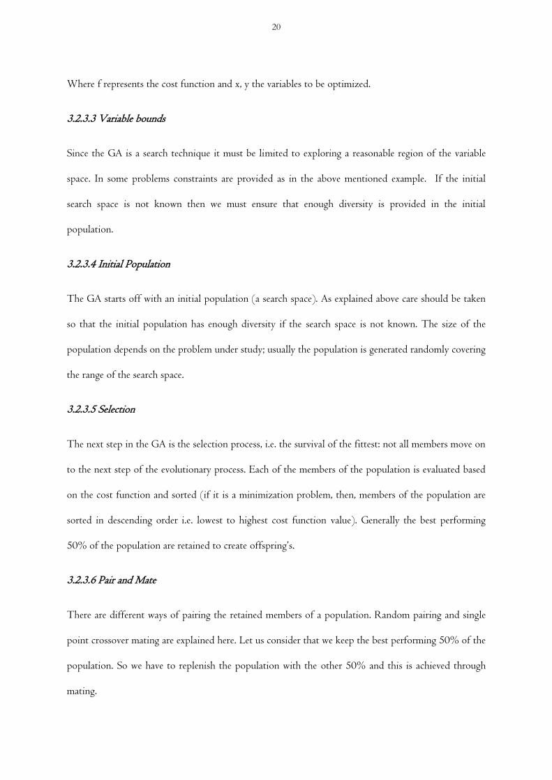
3.2.3.6 Pair and Mate

There are different ways of pairing the retained members of a population. Random pairing and single

point crossover mating are explained here. Let us consider that we keep the best performing 50% of the

population. So we have to replenish the population with the other 50% and this is achieved through

mating.

20

The following example shows how single point crossover works. Assume P1 and P2 are a randomly

selected pair representing the parameters to be optimized (e.g. x and y) and O1, O2 their offspring’s.

Then

P1 = [x1, y1] P2 = [x2, y2]

Possible combinations (pairings) are:

Pairing 1 = [x1, y1] pairing 3 = [x1, y2]

Pairing 2 = [x2, y1] pairing 4 = [x2, y2]

The pairings 1 and 4 represents the parents who are retained while parings 2 and 3 are the

recombination of the parents (offspring) and become the new population members in the next

generation.

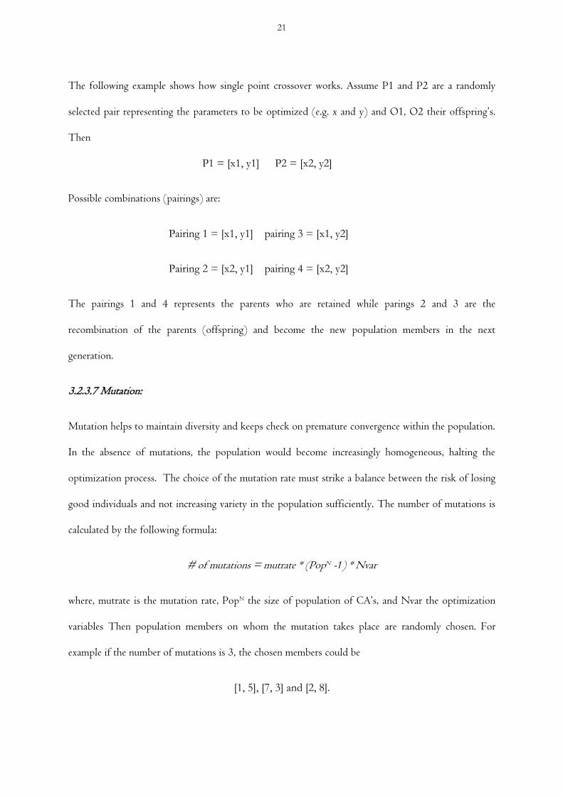
3.2.3.7 Mutation:

Mutation helps to maintain diversity and keeps check on premature convergence within the population.

In the absence of mutations, the population would become increasingly homogeneous, halting the

optimization process. The choice of the mutation rate must strike a balance between the risk of losing

good individuals and not increasing variety in the population sufficiently. The number of mutations is

calculated by the following formula:

# of mutations = mutrate * (PopN -1) * Nvar

where, mutrate is the mutation rate, PopN the size of population of CA’s, and Nvar the optimization

variables Then population members on whom the mutation takes place are randomly chosen. For

example if the number of mutations is 3, the chosen members could be

[1, 5], [7, 3] and [2, 8].

21

If the variables to be optimized can take values between 1 and 10, the mutated members could be

[3, 5], [7, 9] and [4, 8]

3.2.3.8 Next Generation

At the end of this process we have a new population and the cost of each individual is again evaluated

as in step 3.2.3.5.

3.2.3.9 Convergence check

The convergence check keeps track of whether an acceptable solution is reached or a set number of

iterations are exceeded, at which point the algorithm is stopped.

Most GA’s keeps track of the population statistics in the form of mean and best cost for each

generation. This chapter provided a brief introduction to evolutionary computation and more

specifically to genetic algorithms and the various steps involved in genetic algorithms.

The next chapter introduces experimental methods and a brief history of the evolution of experimental

economics.

3.3 EXPERIMENTAL METHODS

I gradually became persuaded that the subjects, without intending to, had revealed to me a basic truth

about markets that was foreign to the literature of economics. Vernon L. Smith

In this section we first introduce experimental methods and then give a quick overview of the history

and foundations of experimental methods and experimental economics.

3.3.1 Introduction

Experimental methods (Friedman and Sunder 1994) can be broadly defined as a scientific approach

where researchers study causal processes in a controlled environment. This scientific approach spans

22

physics, chemistry, psychology, biology and more recently economics. An experiment is a scientific

method which is conducted to test a hypothesis. The first step in any experimental method is problem

definition, i.e. building a hypothesis. Next, an experiment can be conducted to confirm or reject the

hypothesis. These experiments can range from being personal (example: sampling different wines to

select one’s favourite) to highly controlled and sophisticated experiments (example: CERNs large

hadron collider where scientists across the globe try to understand the laws of nature).

3.3.2 An experiment

Figure 3.2 gives a holistic idea regarding the steps involved in an experiment. To go through the steps

we use a very simple example of spontaneous generations as devised by the famous microbiologist

Louis Pasteur. During the 1800’s biologists believed that micro-organisms grew from non-living things

postulating spontaneous generation, i.e. life comes into existence without any medium. So the goal for

Louis Pasteur was to disprove this notion. The problem definition and hypothesis for him were to

contradict spontaneous generation.

The next step is data collection through experiments. Pasteur set up two experiments. In experiment 1

he used a glass flask containing broth with an s-curved spout; he then boiled the flask to kill any

bacteria that might be in it. The flask was then left to see if any micro-organisms grew in them. In

experiment 2 Pasteur used a similar glass flask except that it did not have an s-curved spout. He boiled

this flask like before to kill any bacteria, and left the flask to see if micro-organisms grew in this flask.

Data analysis and interpretation in economics generally involve statistical analysis, but for Pasteur it

was what he observed from his experiments. He found out that in experiment 1 there was no bacterial

growth, whereas in experiment 2 there was bacterial growth. Here the control was the s-curved spout to

check the effect of environment on bacterial (micro-organic) growth. Also Pasteur repeated this

experiment in different locations and environments to ensure that the results were correct.

23

© Michael Lombardi

Figure 3.2: Steps in an experimental method

The final stage of an experimental method is confirming or refuting the hypothesis; Pasteur thus

through his experiment disproved what biologists at his time believed to be spontaneous generation.

In the next section we take a brief peek into the history and foundations of experimental methods and

experimental economics.

3.3.3 History and foundations of experimental methods and experimental economics

The use of experiments to understand theories and principles of nature has always been on shaky

grounds. Physics as we know it now, was considered non-experimental. It took great minds such as

Galileo, Newton and Einstein to introduce the notion of experiments in modern physics. Antoine

Lavoisier helped develop quantitative chemical experiments, thus adding an experimental flavour to

chemistry. Biology for a long time was considered non-experimental as it was a living science (i.e. its

subjects were living organisms). Mendel through his experiment on pea plants and Pasteur through his

Hypothesis

Data collection through

controlled experiments

Data analysis

Interpretation of results.

Confirm or reject hypothesis

Problem

definition

24

experiments to develop vaccines made modern biology experimental. Over the last century we have also

seen the evolution of experimental psychology. A quote from Friedman and Sunder (1994) rightly

explains the development (page 1) “History suggests that a discipline becomes experimental when

innovators develop techniques for conducting relevant experiments. The process can be contagious,

with advances in experimental technique in one discipline inspiring advances elsewhere.”

Experimental methods in economics were shunned and considered impractical. But over the last few

decades we have seen the transformation and the use of experimental methods in economics. The use of

experiments in economics came into the picture mainly due to the innovative scientific approaches

(statistics, mathematics, and computer simulations) that were used to study the real world economy

(Guala, 2008). Von Neumann and Morgenstern’s Theory of Games and Economic behaviour (2007)

and development of game theory and decision theory set the ball rolling for experimental economics.

Princeton University’s mathematicians between the 40’s and 60’s used game theoretical puzzles to back

up their theoretical claims. Schelling’s “The strategy of conflict” (Schelling, 2005) is an example of this

development. Siegel and Fouraker (1960) tried to combine economics and psychology to understand

bargaining behaviour. Siegel and Fourakers’ experiments introduced the idea of using real incentives

and also the implementation of strict between-subject anonymity (Guala, 2008). Herber Simon is

considered to be a source of inspiration for the development of experimental economics. Selten, a

trained economist and mathematician who also understood experimental psychology, put together von

Neumann and Morgenstern’s work along with Simon’s bounded rationality to contribute towards

social science research (Guala, 2008).

Experimental economics owes its much acclaimed usage and presence to the work of Smith (1982;

1989). Smith and Charles Plott were instrumental in setting the rules for experimental design and put

forth the ideas of economic experiments. For a detailed reading on the history of experimental

economics refer to Guala (2008).

25

The literature on experimental methods in economics (Friedman and Sunder, 1994) focuses on three

basic principles that need to be followed while designing an experiment: 1) Realism, this refers to the

difference that generally exists between simulation models and experiments. Sterman (1987) talks about

this difference by pointing to the fact that simulation models can capture the physical structure of the

system under study, but decision rules of these models must correspond to the actors who use them.

Most of the models in general are governed by rules set by the modeller and not by the agents who use

them. Experimental economics should try to bridge the gap that exists between models and reality

(Grossklags, 2007). 2) Control and repetition; a control is needed in the experiment in order to

observe the effects of a variable under study (this is what we call treatments). Control ensures that the

experimental data is a result of manipulations made by the experimenter in the experimental

environment. Repetition on the other hand is needed to have a check on the variability observed in the

data. 3) Induced-value theory; Friedman and Sunder point out that the key idea behind induced-value

theory is to “induce” pre-specified characteristics in subjects. To accomplish this, experimenters should

come up with a reward mechanism that conveys the message to subjects, that the reward they receive is

related to their performance and not allowing them to be satiated. These are the three important

principles that need to be kept in mind while designing experiments. For a detailed reading on this

topic refer to Friedman and Sunder, 1994.

Chapter 3 introduced the methodologies that have been adopted in this thesis. Main contributors and

basic ideas behind these methodologies have been described. There might be other contributors and

techniques that have not been discussed. For detailed readings refer to the bibliography.

The next chapter is a collection of three scholarly papers that presents the contribution of the thesis

towards the study of behavioural queuing systems.

26

CHAPTER 4 PAPERS

4.1 THE MICRO-DYNAMICS OF QUEUING: UNDERSTANDING THE FORMATION OF

QUEUES

(with Carlos Delgado, Erik R Larsen and Ann van Ackere)

ABSTRACT

Most work in queuing theory is performed at an aggregate level, with linear models for which closed

form solutions can be derived. We are interested in creating a better understanding of how queues are

formed by taking a bottom-up approach to their formation. We use a cellular automata framework to

structure a set of agents who must choose which service facility to use. After using the facility, they

update their expectations of sojourn time based on their own experience, and information received from

their neighbors’. Based on these updated expectations, they make their choice for the next period. We

find that, after an initial transition period, customers mostly reach a quasi-stable situation, where the

average sojourn time is close to the Nash equilibrium and social optimum, unless agents forget one of

the facilities. We analyze different parameterizations’ of the agents' decision rules, and consider

homogeneous and heterogeneous agent populations.

INTRODUCTION

Queuing theory has since its inception mainly dealt with an aggregated or systems level view of the

processes involved. Typically, customers arrive following a stochastic process, in many cases a Poisson

process; after waiting a certain time they receive service and then disappear, not to be seen again (Gans

and Zhou, 2003; Gross and Harris, 1998). The focus was on being able to establish a closed form

solution for the model, which implies that the model is linear, and the main objective was to find the

"optimal" capacity of the service facility, i.e. the capacity that maximizes profit or welfare. There have

been noteworthy exceptions from this general scheme, such as Haxholdt et al. (2003) and Law et al

(2004) . More recently there has been a movement towards studying behavioral issues in operations

27

management (Gino and Pisano, 2008; (Bendoly et al., 2010), which has to some (limited) extent also

impacted queuing research. This work includes a number of empirical studies, mainly in the area of

service marketing (A. K.Y. Law et al., 2004), where researchers have studied the effect of queuing on

return rates to the same outlets. Theoretical work has looked at including feedback into the models, so

that customers may decide to return or not to the same service facility (Haxholdt et al., 2003, van

Ackere et al., 2006). Finally, some experimental studies have also begun to question certain taken for

granted assumptions in queuing (Bielen and Dumoulin, 2007). Still, very little has been done to

attempt to understand the impact of individual decision making; i.e. how does individual expectation

formation affect the creation and dissolution of queues, and the selection of service facilities based on

past experience?

In this paper, we begin to address these issues by looking at how individuals form expectations, and

how the interactions of individuals influence the formation of queues. We develop an agent based

model which represents a population of decision makers who repeatedly have to make a choice about

which service facility to use. After choosing a service provider and experiencing the actual sojourn time,

they update their expectations based on this new experience, and take this into account when making a

choice for the next period. We structure the agents in a cellular automaton, to be able to define a

neighborhood and the interactions between the individual agents / decision makers. Our model can be

seen as a collective choice model with negative externalities, as an agent does not know the choice of the

other agents when making a decision; however, these other agents' choices of service facility

significantly influence the resulting sojourn times.

Using a disaggregated agent based framework (e.g. cellular automata) provides a number of advantages

over the more traditional approach when aiming to understand the micro dynamics of the formation of

queues. While each agent makes a locally rational choice, the macro (aggregated) dynamics might be far

away from the optimum. This is similar to the micro-macro problem in the social sciences (or forward-

28

backward problems in physics, see Gutowitz, 1991). We can study the aggregated outcome of the way

in which individual agents form expectations, e.g. how they update their expectations based on

experience and the effect of information in the system. This allows us to get an insight into better ways

of designing service facilities, compared to the more traditional “top-down” approach which tries to

infer the individual behavior from the aggregated data. The latter task is in most cases impossible,

unless strict neoclassical (unrealistic) conditions are assumed.

Such a micro foundation approach has been used in other areas, including traffic where detailed studies

of how the aggregated traffic builds on individual choices of travel routes have helped shed new light

on the effect of road restrictions (one-way systems, design of exits etc) (Benjamin et al., 1996). In

physics and biology, agent based models have likewise improved both theoretical and practical

understanding of a number of phenomena (Deutsch and Dormann, 2005); in the social science they

have been used in areas such as sociology (Caruso et al., 2007), management (Lomi and Larsen, 1996)

and many others.

In this paper we develop a model of individual choice, where each agent decides each period which

service facility to use. Having used the chosen facility, agents update their expectation of the sojourn

time for that service facility and use information from other agents they communicate with to update

expectations about other service facilities. The next period, the agents again choose which service

facility to use based on these updated expectations. We study how the agents adjust to the system and

to each other as time evolves, as the sojourn times depend on the number of agents choosing each

station that period. The next section describes the motivation and the development of the model. This

is followed by a discussion of the simulation results, while the final section contains our concluding

comments and suggestions for further work.

MODEL DESCRIPTION

We consider a group of customers who, each period, must choose which service facility (referred to as

29

queues) to patronize. They make their choice based on the sojourn time which they expect to face at

the different facilities. We model this situation using a one-dimensional cellular automaton (CA)

(Gutowitz, 1991; Wolfram, 1983; 1994) which assumes local interactions between intelligent adaptive

agents. We call the agents intelligent because they have a memory (expectation) which contains the

expected sojourn time for each facility.

We assume a ring structure wherein each cell of the CA represents an agent. Each agent has exactly two

neighbors’, one on each side. The parameter K defines the number of neighbors (referred to as the K-

neighborhood (Lomi et al., 2003)) from whom there is information diffusion. The neighborhood

represents for instance a social network encompassing colleagues, friends, people living next-door etc.

As an example, if K = 1 and A is a set of N agents {A1, A2,…, Ai,…, AN }, then agent Ai will interact

with agents Ai-1 and Ai+1.

We use the following notation: there are N agents, who each period choose one of Q queues. Each

queue has a service rate μ and an arrival rate λjt. Note that μ is exogenous and common to all queues,

whereas λjt is endogenous and represents the number of agents choosing queue j in period t. At the end

of a period, each agent updates his expectation of the sojourn time based on two sources of

information: his own experience, and that of his neighbors’ (van Ackere and Larsen, 2004). Based on

his own experience, he will update his estimate of the sojourn time at his chosen service station using an

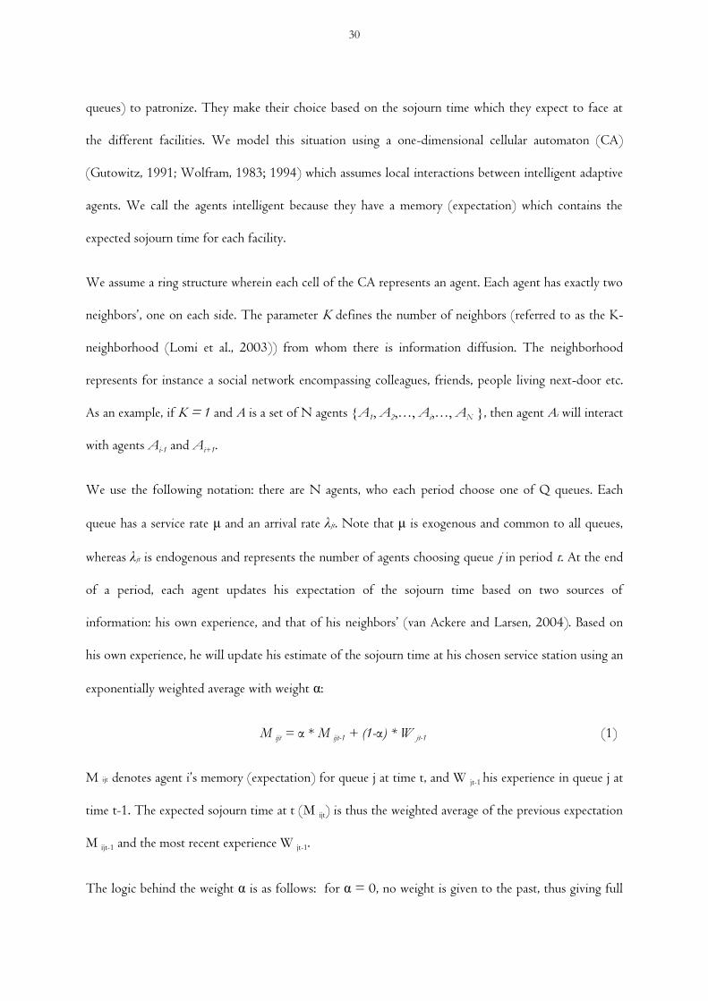
exponentially weighted average with weight α:

M ijt = α * M ijt-1 + (1-α) * W jt-1 (1)

M ijt denotes agent i’s memory (expectation) for queue j at time t, and W jt-1 his experience in queue j at

time t-1. The expected sojourn time at t (M ijt) is thus the weighted average of the previous expectation

M ijt-1 and the most recent experience W jt-1.

The logic behind the weight α is as follows: for α = 0, no weight is given to the past, thus giving full

30

weight to the most recent experience. A value of α = 1 implies inertia, i.e. no updating of expectations.

Thus, the higher the value of α, the more conservative the agent is towards new information, while a

lower value means agents consider their recent experiences to be more relevant. This updating method

is known as adaptive expectations (Nerlove, 1958) or exponential smoothing (Gardner, 2006).

The second source of information comes from the experience of the agent's neighbors’. The agent

checks which neighbor experienced the shortest sojourn time at time t-1. Using the same logic as

described above for his own experience, the agent will update his expectation for the queue used by this

neighbor using parameter β. In the special case where the facility chosen by the agent and that chosen

by his best performing neighbor coincide, the agent only updates his expectation once, using the

minimum of α and β as weight. The queue for the next period is chosen based on these updated

expectations. In case of a tie between two or more facilities, he will in order of preference stay where he

was, select the facility used by his neighbor, or choose randomly. To summarize, the flow of the model

is as follows: at time t = 0, agents are allocated randomly to a queue, with each queue having equal

probability. They experience a sojourn time and learn about their neighbors’ experience. They update

their expectation based on this information and use these updated expectations to select the queue with

the shortest expected sojourn time for period 1. These new choices lead to new experiences and

information, and the updating and decision process is repeated.

Next we need to define the sojourn time W jt at queue j at time t, given that λ jt agents selected this

queue. Let us consider an M/M/1 system (i.e. a one-server system with Poisson arrivals and

exponential service times, see e.g. Gross and Harris, 1998) in steady state. For such a system, the

expected number of people in the system (L) satisfies equation (2):

1L (2)

where ρ denotes the utilization rate λ/μ. Recalling the well-known Little’s law

31

L = λ * W (3)

equations (2) and (3) imply that W equals

1W . (4)

Unfortunately, these equations are only valid in steady state, which requires ρ < 1. We need a

congestion measure which can be used for a transient analysis where at peak times the arrival rate

temporarily exceeds the service rate. Consider for instance the case of a toll bridge where during peak

time there is clustering of commuters: it takes a while for this queue to disappear. We have therefore

attempted to identify a congestion measure that satisfies the behavioral characteristics of equations (2)

to (4), but remains well-defined when ρ ≥ 1. Such a measure should satisfy the following criteria:

(i) If ρ equals zero, the number of people in the facility, L, equals zero (Equation 2);

(ii) L increases more than proportionally in ρ (Equation 2);

(iii) When the arrival rate tends to zero, the sojourn time W is inversely proportional to the service

rate µ (Equation 4);

(iv) When the arrival rate and service rate increase proportionally, leaving ρ unchanged,

the waiting time W decreases (Equations 2 and 3);

(v) Little's Law is satisfied (Equation 3).

With these requirements in mind, we define L jt as follows:

jtjtjtjtjtL 2)1( . (5)

Using Little's law and the definition of ρ yields the average sojourn time

μ

+μ

jtλ=jtW

1

2. (6)

32

Experimental Setup

Cellular automata are used in many disciplines as a way of modeling a variety of phenomena from

coffee speculation and traffic models to the growth of organizational populations (Bandini et al., 1997;

Lomi and Larsen, 1996; Wahle et al., 2001). The agents of a CA model are endowed with memory,

which makes this framework more suitable for investigating our problems. We model the agents’

memory using adaptive expectations as described above. As our model cannot be solved analytically, we

turn to simulation as a method of analysis. We use a CA with 120 agents (cells) and 3 facilities (states),

an adequate size to observe the phenomena we are concerned with. We also experimented with a larger

number of agents; this did not change the results in any significant way.

Each agent is allocated an initial memory for the expected sojourn time for each facility; these

memories are distributed randomly around the optimal average sojourn time. We simulate the models

for 50 periods, which is sufficient to show the development of the automata and (in most cases) reach a

form of steady state (i.e. the behavior remains the same for longer simulations). We have run much

longer simulations to verify this. The agents choose between three identical facilities. It is important to

note that all agents choosing a specific facility experience the same sojourn time, i.e. we do not consider

order of arrival: we report the average sojourn time. This is also consistent with our assumption of

simultaneous choice and synchronous updating of the agents. The parameters used in the simulation are

shown in table 4.1. Given that the three facilities are identical, the social optimum and the Nash

equilibrium coincide and correspond to the case where agents are equally distributed, 40 choosing each

of the three facilities. This results in a sojourn time of 1.8 time units.

RESULTS

We present aggregated results before giving a more detailed discussion of the behavior of individual

agents. Figure 4.1 shows the spatial-temporal evolution of the automaton: the agents are on the y-axis

33

and the x-axis represents time. The colors indicate the chosen facility of a particular agent at a given

time (black = facility 1, grey = facility 2, white = facility 3). We see that initially the agents try out

different facilities depending on their randomly allocated initial expectations. In the first few time

periods different facilities are tested, e.g. at time = 4 the majority chose facility 2 (grey), thus

generating a long sojourn time. Consequently, in the following period (time 5) no agents use facility 2,

Parameter

Value

Description

Q

3

Number of service facilities

N

120

Population size (Number of agents)

μ

{5,5,5}

Service rate

α

{0-1}

Weight to memory w.r.t. own experience

β

{0-1}

Weight to memory w.r.t. neighbors’ experience

Tsim

50

Simulation time

K

1

Neighborhood Size

Table 4.1: Parameter values used for the base case as well as the range used for experiments.

-and most turn to facility 1 (black). This transitional behavior continues until time 10. Next, a set of

more stable choices emerges over the next 5 time periods. After period 15, the majority of agents stay

with the same facility for the remaining 35 periods, while a minority keeps switching between two

different facilities. E.g. agent 80 switches between facilities 1 and 2 in a fairly regular pattern. Agents

switching between 2 facilities (note that none switches between all three facilities) create the boundaries

for the "stable" agents: the information thus provided removes any incentive to switch.

In Figure 4.2a we observe the evolution of the average sojourn time for the system as well as the

minimum and maximum across the three queues. Referring to what we observed in figure 4.1, we see

that in the transition phase the average sojourn time occasionally peaks near 4.0, which is more than

twice the Nash equilibrium value of 1.8. These peaks occur when the agents are clustered in two

queues. From period 15 onwards, the average travel time is almost constant, with only very minor

34

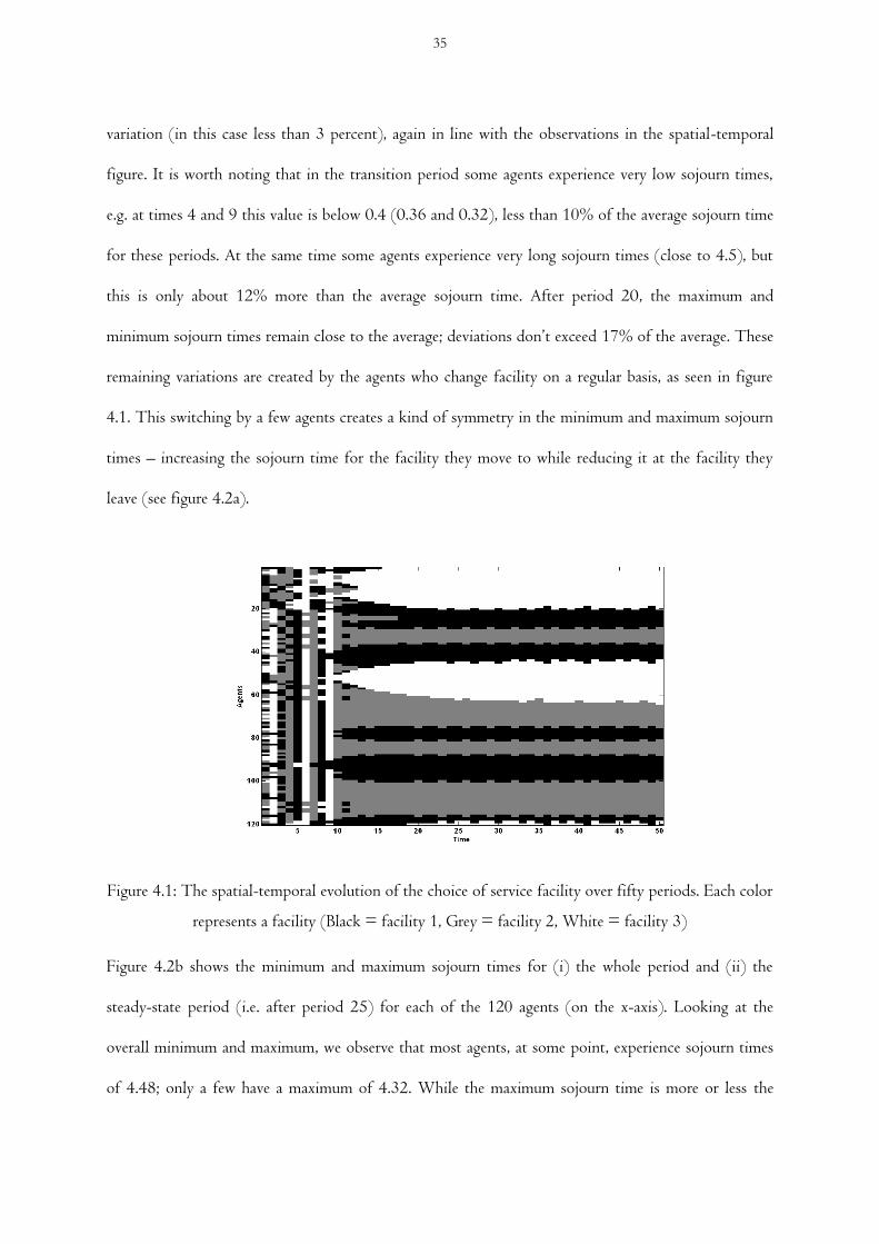
variation (in this case less than 3 percent), again in line with the observations in the spatial-temporal

figure. It is worth noting that in the transition period some agents experience very low sojourn times,

e.g. at times 4 and 9 this value is below 0.4 (0.36 and 0.32), less than 10% of the average sojourn time

for these periods. At the same time some agents experience very long sojourn times (close to 4.5), but

this is only about 12% more than the average sojourn time. After period 20, the maximum and

minimum sojourn times remain close to the average; deviations don’t exceed 17% of the average. These

remaining variations are created by the agents who change facility on a regular basis, as seen in figure

4.1. This switching by a few agents creates a kind of symmetry in the minimum and maximum sojourn

times – increasing the sojourn time for the facility they move to while reducing it at the facility they

leave (see figure 4.2a).

Figure 4.1: The spatial-temporal evolution of the choice of service facility over fifty periods. Each color

represents a facility (Black = facility 1, Grey = facility 2, White = facility 3)

Figure 4.2b shows the minimum and maximum sojourn times for (i) the whole period and (ii) the

steady-state period (i.e. after period 25) for each of the 120 agents (on the x-axis). Looking at the

overall minimum and maximum, we observe that most agents, at some point, experience sojourn times

of 4.48; only a few have a maximum of 4.32. While the maximum sojourn time is more or less the

35

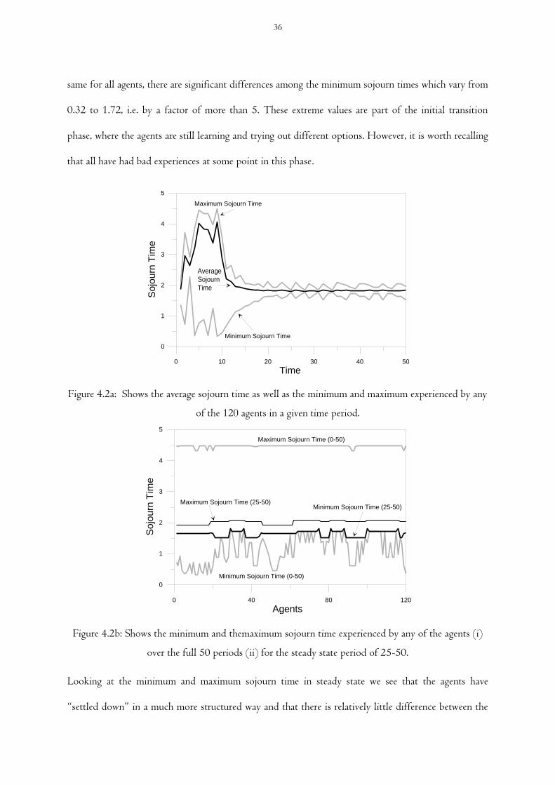
same for all agents, there are significant differences among the minimum sojourn times which vary from

0.32 to 1.72, i.e. by a factor of more than 5. These extreme values are part of the initial transition

phase, where the agents are still learning and trying out different options. However, it is worth recalling

that all have had bad experiences at some point in this phase.

0 10 20 30 40 50

Time

0

1

2

3

4

5

Sojo

urn

Tim

e

Maximum Sojourn Time

Minimum Sojourn Time

Average Sojourn Time

Figure 4.2a: Shows the average sojourn time as well as the minimum and maximum experienced by any

of the 120 agents in a given time period.

0 40 80 120

Agents

0

1

2

3

4

5

Sojo

urn

Tim

e

Maximum Sojourn Time (0-50)

Maximum Sojourn Time (25-50)Minimum Sojourn Time (25-50)

Minimum Sojourn Time (0-50)

Figure 4.2b: Shows the minimum and themaximum sojourn time experienced by any of the agents (i)

over the full 50 periods (ii) for the steady state period of 25-50.

Looking at the minimum and maximum sojourn time in steady state we see that the agents have

“settled down” in a much more structured way and that there is relatively little difference between the

36

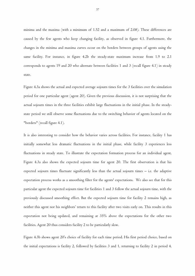
minima and the maxima (with a minimum of 1.52 and a maximum of 2.08). These differences are

caused by the few agents who keep changing facility, as observed in figure 4.1. Furthermore, the

changes in the minima and maxima curves occur on the borders between groups of agents using the

same facility. For instance, in figure 4.2b the steady-state maximum increase from 1.9 to 2.1

corresponds to agents 19 and 20 who alternate between facilities 1 and 3 (recall figure 4.1) in steady

state.

Figure 4.3a shows the actual and expected average sojourn times for the 3 facilities over the simulation

period for one particular agent (agent 20). Given the previous discussion, it is not surprising that the

actual sojourn times in the three facilities exhibit large fluctuations in the initial phase. In the steady-

state period we still observe some fluctuations due to the switching behavior of agents located on the

"borders" (recall figure 4.1).

It is also interesting to consider how the behavior varies across facilities. For instance, facility 1 has

initially somewhat less dramatic fluctuations in the initial phase, while facility 3 experiences less

fluctuations in steady state. To illustrate the expectation formation process for an individual agent,

Figure 4.3a also shows the expected sojourn time for agent 20. The first observation is that his

expected sojourn times fluctuate significantly less than the actual sojourn times – i.e. the adaptive

expectation process works as a smoothing filter for the agents' expectations. We also see that for this

particular agent the expected sojourn time for facilities 1 and 3 follow the actual sojourn time, with the

previously discussed smoothing effect. But the expected sojourn time for facility 2 remains high, as

neither this agent nor his neighbors’ return to this facility after two visits early on. This results in this

expectation not being updated, and remaining at 35% above the expectations for the other two

facilities. Agent 20 thus considers facility 2 to be particularly slow.

Figure 4.3b shows agent 20’s choice of facility for each time period. His first period choice, based on

the initial expectations is facility 2, followed by facilities 3 and 1, returning to facility 2 in period 4,

37

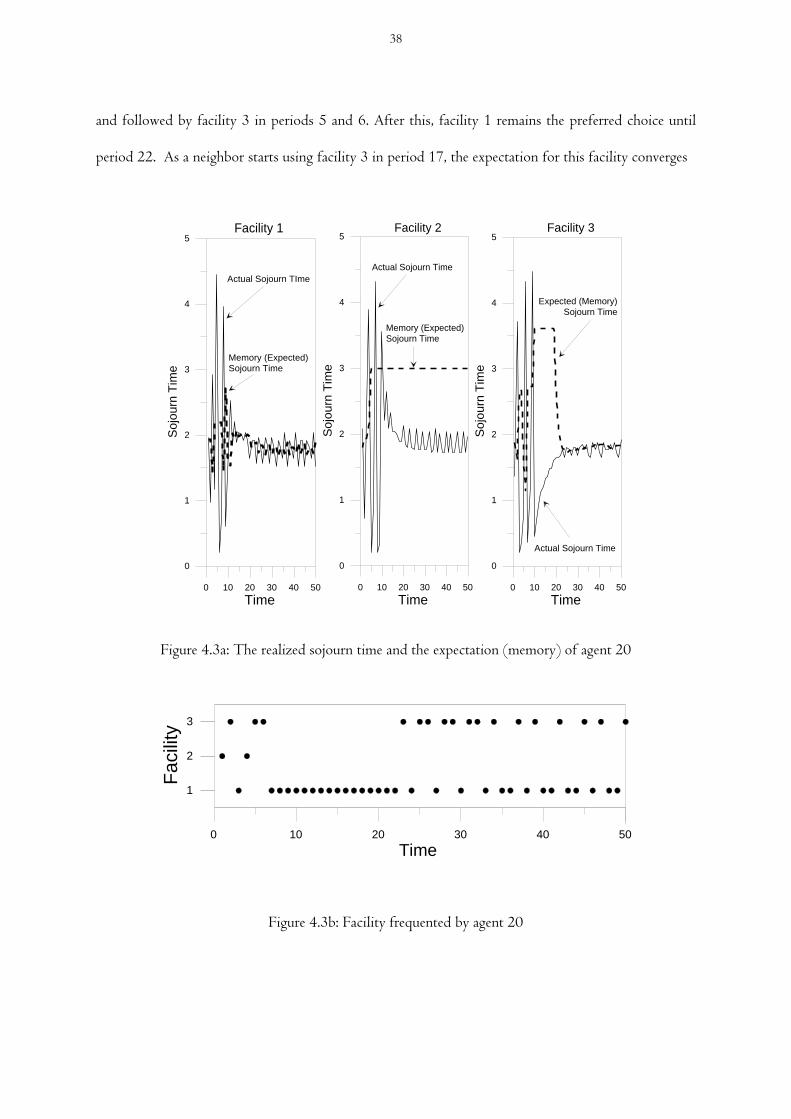
and followed by facility 3 in periods 5 and 6. After this, facility 1 remains the preferred choice until

period 22. As a neighbor starts using facility 3 in period 17, the expectation for this facility converges

0 10 20 30 40 50

Time

0

1

2

3

4

5

So

journ

Tim

e

Actual Sojourn TIme

Memory (Expected)

Sojourn Time

Facility 1

0 10 20 30 40 50

Time

0

1

2

3

4

5

So

journ

Tim

e

Actual Sojourn Time

Memory (Expected)

Sojourn Time

Facility 2

0 10 20 30 40 50

Time

0

1

2

3

4

5

So

journ

Tim

e

Actual Sojourn Time

Expected (Memory)

Sojourn Time

Facility 3

Figure 4.3a: The realized sojourn time and the expectation (memory) of agent 20

0 10 20 30 40 50

Time

1

2

3

Fa

cili

ty

Figure 4.3b: Facility frequented by agent 20

38

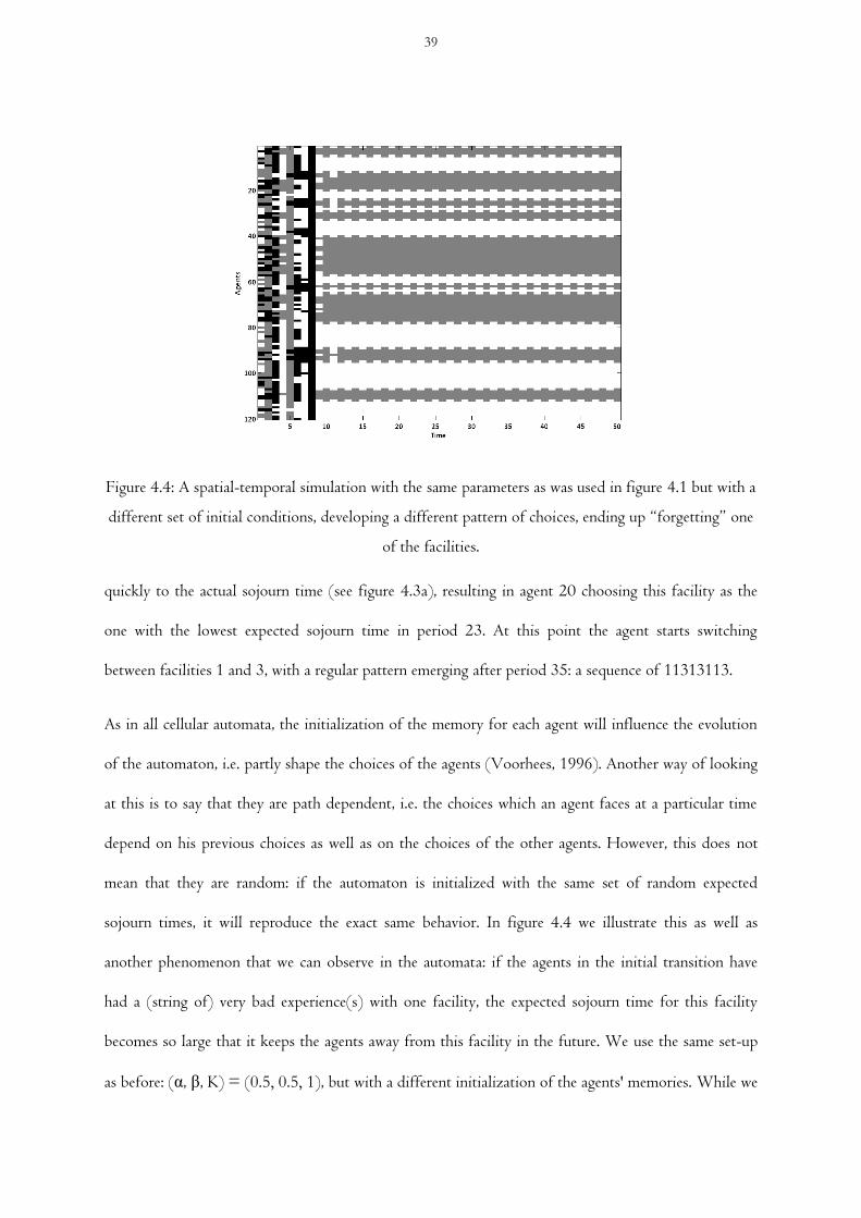
Figure 4.4: A spatial-temporal simulation with the same parameters as was used in figure 4.1 but with a

different set of initial conditions, developing a different pattern of choices, ending up “forgetting” one

of the facilities.

quickly to the actual sojourn time (see figure 4.3a), resulting in agent 20 choosing this facility as the

one with the lowest expected sojourn time in period 23. At this point the agent starts switching

between facilities 1 and 3, with a regular pattern emerging after period 35: a sequence of 11313113.

As in all cellular automata, the initialization of the memory for each agent will influence the evolution

of the automaton, i.e. partly shape the choices of the agents (Voorhees, 1996). Another way of looking

at this is to say that they are path dependent, i.e. the choices which an agent faces at a particular time

depend on his previous choices as well as on the choices of the other agents. However, this does not

mean that they are random: if the automaton is initialized with the same set of random expected

sojourn times, it will reproduce the exact same behavior. In figure 4.4 we illustrate this as well as

another phenomenon that we can observe in the automata: if the agents in the initial transition have

had a (string of) very bad experience(s) with one facility, the expected sojourn time for this facility

becomes so large that it keeps the agents away from this facility in the future. We use the same set-up

as before: (α, β, K) = (0.5, 0.5, 1), but with a different initialization of the agents' memories. While we

39

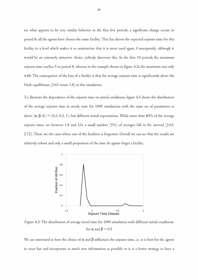
see what appears to be very similar behavior in the first few periods, a significant change occurs in

period 8: all the agents have chosen the same facility. This has driven the expected sojourn time for this

facility to a level which makes it so unattractive that it is never used again. Consequently, although it

would be an extremely attractive choice, nobody discovers this. In the first 10 periods the maximum

sojourn time reaches 5 in period 8, whereas in the example shown in figure 4.2a the maximum was only

4.48. The consequence of the loss of a facility is that the average sojourn time is significantly above the

Nash equilibrium (2.65 versus 1.8) in this simulation.

To illustrate the dependence of the sojourn time on initial conditions, figure 4.5 shows the distribution

of the average sojourn time in steady state for 1000 simulations with the same set of parameters as

above (α, β, K) = (0.5, 0.5, 1), but different initial expectations. While more than 80% of the average

sojourn times are between 1.8 and 2.0, a small number (5%) of averages fall in the interval [2.65,

2.72]. These are the cases where one of the facilities is forgotten. Overall we can see that the results are

relatively robust and only a small proportion of the time do agents forget a facility.

1.5 2 2.5 3

Sojourn Time Classes

0

0.2

0.4

0.6

0.8

1

Fra

ction o

f A

ll R

un

Figure 4.5: The distribution of average travel time for 1000 simulation with different initial conditions

for α and β = 0.5

We are interested in how the choice of α and β influences the sojourn time, i.e. is it best for the agents

to react fast and incorporate as much new information as possible or is it a better strategy to have a

40

higher level of inertia and only slowly update the expectations? We therefore vary α from 0 to 1 in

increments of 0.1, and for each α we consider 5 different values of β: 0.0, 0.3, 0.5, 0.7, and 1.0. As

discussed above, the average sojourn time is influenced by the initial randomly allocated expectations of

sojourn times for the different facilities. To account for this we run 1000 iterations for each of these

(α, β) combinations and calculate the average and the standard deviation of the sojourn times. The

averages are shown in figure 4.6.

The first observation is that, except for β equal to 1.0, the average sojourn time decreases in α for

values below 0.6, then remains fairly constant, and finally increases once α reaches 0.9. In other words,

up to a certain point, a slower updating of the expectations based on the agents' own experience

generally leads to a better overall performance of the automaton. For β equal to 1.0, the average sojourn

time decreases in α.

0 0.2 0.4 0.6 0.8 1

1.5

2

2.5

3

Ave

rage

So

jou

rn T

ime

= 0.0

= 0.3

= 0.5 = 0.7

= 1.0

Figure 4.6: The average sojourn time as a function of α for selected values of β. Each recorded values

of α represents the average of 1000 simulations with different initial values. Note that for reasons of

legibility the Y-axis starts at 1.5.

41

Taking a closer look at the influence of β on the resulting sojourn time, we see that, at least until α

reaches 0.9, the worst we can do is to adopt one of the “extreme” updates with β = 1 or β = 0, i.e.

substituting the expectations with the neighbors’ new experience or ignoring this information. Both of

these lead to equally poor results, unless α is close to 1: in some cases the average sojourn time is 40%

higher than the best among the 5 selected β values. It is also clear that extremely fast updating of

expectations using the agents’ own experience is worse than no updating. The difference in performance

among the three other values of β is much smaller across most of the α range: only a few percent until

α reaches 0.8. Overall the best values are obtained with a relatively high α and a medium β. In other

words, more conservative agent populations who have a certain degree of skepticism with regard to the

most recent experiences are doing better than populations who follow an aggressive strategy and put

much weight on the current experience.

Next we run two experiments where α and β are respectively relatively small (both 0.1) and quite large

(0.9). The first case implies that the agents' memory is updated very fast. In the second case agents put

little emphasis on the current experience but rely on their past experience, i.e. their expectations.

In the first case, agents react very strongly to the experienced sojourn time: a single bad experience can

turn them off a specific facility forever. Consequently it is fairly common that by the time steady state

is reached, one of the facilities is forgotten. This implies that on average, such populations perform

rather poorly. In those instances where they avoid this trap, their average sojourn time is close to the

Nash equilibrium. Figures 4.7a and 4.7b show such a case. The fast updating implies that behavior is

quite volatile during the transition period, but the agents quickly converge to a steady state: the average

sojourn time equals 1.835, and the behavior is similar to the base case.

Figure 4.7c illustrates the case where α and β are equal to 0.9. The very slow updating of expectations

is reflected in a very fragmented distribution of facility choice, there is no coherence of fairly large

groups of neighbors’ making the same choice as in the base case and in for small α and β values.

42

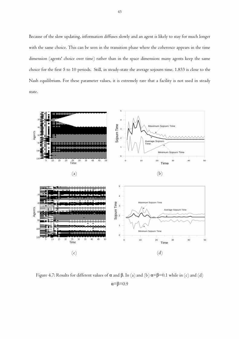
Because of the slow updating, information diffuses slowly and an agent is likely to stay for much longer

with the same choice. This can be seen in the transition phase where the coherence appears in the time

dimension (agents' choice over time) rather than in the space dimension: many agents keep the same

choice for the first 5 to 10 periods. Still, in steady-state the average sojourn time, 1.833 is close to the

Nash equilibrium. For these parameter values, it is extremely rare that a facility is not used in steady

state.

0 10 20 30 40 50

Time

0

1

2

3

4

5

Sojo

urn

Tim

e

Maximum Sojourn Time

Average Sojourn Time

Minimum Sojourn Time

(a) (b)

0 10 20 30 40 50

Time

0

1

2

3

4

5

Sojo

urn

Tim

e Maximum Sojourn Time

Minimum Sojourn Time

Average Sojourn Time

(c) (d)

Figure 4.7: Results for different values of α and β. In (a) and (b) α=β=0.1 while in (c) and (d)

α=β=0.9

43

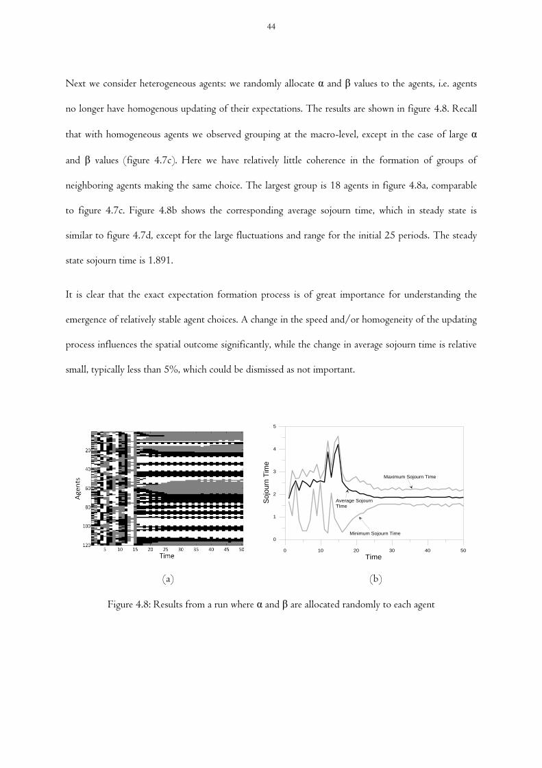
Next we consider heterogeneous agents: we randomly allocate α and β values to the agents, i.e. agents

no longer have homogenous updating of their expectations. The results are shown in figure 4.8. Recall

that with homogeneous agents we observed grouping at the macro-level, except in the case of large α

and β values (figure 4.7c). Here we have relatively little coherence in the formation of groups of

neighboring agents making the same choice. The largest group is 18 agents in figure 4.8a, comparable

to figure 4.7c. Figure 4.8b shows the corresponding average sojourn time, which in steady state is

similar to figure 4.7d, except for the large fluctuations and range for the initial 25 periods. The steady

state sojourn time is 1.891.

It is clear that the exact expectation formation process is of great importance for understanding the

emergence of relatively stable agent choices. A change in the speed and/or homogeneity of the updating

process influences the spatial outcome significantly, while the change in average sojourn time is relative

small, typically less than 5%, which could be dismissed as not important.

0 10 20 30 40 50

Time

0

1

2

3

4

5

Sojo

urn

Tim

e

Minimum Sojourn Time

Maximum Sojourn Time

Average Sojourn

TIme

(a) (b)

Figure 4.8: Results from a run where α and β are allocated randomly to each agent

44

CONCLUSION

We have discussed how it is possible to begin to investigate the micro foundation for queuing by

defining and studying the formation of expectations for single agents and the macro consequences for

the system. While queuing systems have mainly been studied at the aggregated level, with customers

arriving following an externally defined distribution, and without repeat service, we are interested in

how the structure and interaction of the individual customers create queues at the service locations and

in particular how repeated experiences influence the formation of these queues.

We can conclude that populations who update their expectations extremely fast using the agents’ own

experience generally perform poorly. Overall, agents who treat new information from their neighbors

cautiously but have sufficient trust in their own experience are more likely to perform well.

While the aggregated outcomes of our simulations show that there are differences in the average

sojourn time, these are relatively small, but these are the differences that queuing typically has been

focusing on. What we have shown is that although there is relatively little difference in the average

sojourn time, there are great differences in the spatial temporal dimension and in the formation of the

individual agents' expectations and choices. These differences are not yet well understood and need to

be investigated in more detail. By looking at the individual level we can begin to get a better

understanding of how information should be distributed and targeted to different agents who have to

decide which facility to use. This is potentially relevant for a wide range of service facilities, ranging

from traffic modes to supermarkets.

The next step is to verify the model using an experimental approach, to get a better understanding of

the actual decision making process. Another aspect is introducing more choice in the model, in

particular timing. This would allow agents to also decide when to use the facility, i.e. introducing a

tradeoff between the preferred time (leaving at 8am) and the shortest sojourn time (leaving before

7am).

45

4.2 MODELLING DECISION MAKING IN AN AGENT BASED QUEUING

SYSTEM USING CELLULAR AUTOMATA AND GENETIC ALGORITHMS.

(with Erik R Larsen and Ann van Ackere)

ABSTRACT

In this paper we propose an agent based framework based on genetic algorithms (GA). In section 4.1,

we introduced an agent based framework using cellular automata (CA). The CA model equips agents

with information and decision making capabilities. The GA model in this paper takes the agent based

framework one step further, and models the learning of populations as they experience the

consequences of queuing. Through the GA we model how populations evolve, and optimize their

behavior based on their experiences.

INTRODUCTION

Queuing research has since the seminal paper by Agner Krarup Erlang (1909) been studied extensively

with an aggregated view of the processes involved. The design and performance of the facility under

study have been the focus of most studies, with the customers using the facility arriving following a

known exogenous distribution. However, many queuing situations are repeated choices among several

facilities based on previous experiences. There has been an increasing interest in this type of behavioral

studies in operations management, for example empirical studies in service marketing (A. K.Y. Law et

al., 2004; Bielen and Demoulin, 2007), which concentrate on the impact of queue length on the return

rate of customers. Of late a number of theoretical models include feedback to understand customers'

satisfaction and its effect on the customers' decision to return to the facility (Haxholdt et al., 2003; van

Ackere et al., 2006). In spite of all these models and research, little attention has been given to the

impact of individual choice on queue formation and understanding of the effects of expectations and

experiences.

46

In this paper we deviate from the traditional approaches of queuing and model customers who evolve

and optimize their behavior based on their experiences using genetic algorithms. Genetic algorithms

(Goldberg, 2009; Haupt and Haupt, 2004b; Holland, 2001; Mitchell, 2001) are a very commonly

used evolutionary computation based optimization technique. GA’s have been used successfully in a

variety of applications including solving the traveling salesman problem (Moon et al., 2002),

operational research (Reeves, 1997), game theoretical models (Hurd and Hamblin, 2007),

organizational theory (Bruderer and Singh, 1996) and engineering optimization (Gen and Cheng,

1997).

This paper builds on the paper presented in section 4.1, and looks into collective learning i.e. the model

optimizes the overall performance of the system. This model is a step further in the design of

intelligent decision makers. Similar to the paper in section 4.1 we incorporate previous experience into

the model by using adaptive expectations (Nerlove, 1958). Agents use adaptive expectations for

updating their expectations regarding sojourn time; and this information is used to choose among

several alternative facilities. The model presented in section 4.1 and this model applies to situations

where customers routinely require a service. Their loyalty, i.e. the decision to return to the facility, is

dependent on their past experiences. A few examples of these situations include person who goes

monthly to the bank, a person who goes to supermarkets on a weekly basis, and a person who

commutes every day to work (choosing alternative routes) among others.

The paper is organized as follows. The methodology section after this brief introduction presents the

model. This is followed by the results section where we provide illustrative examples to highlight the

proposed approach, and a concluding discussion section.

47

METHODOLOGY

In this paper we consider a group of customers, who routinely choose a facility from a multi-channel

system. The choice of the service facility is based on their expectations of sojourn time and the

information available to them through a network (local interactions). This network, called

neighborhood, could be envisioned as a social network consisting of friends, family members,

colleagues, neighbors etc. and also physical networks.

We model this evolving/learning agent based framework by using a combination of a one dimensional

Cellular automata (CA) (Gutowitz, 1991; Wolfram, 1983; Wolfram, 1984; Wolfram, 2002) and

Genetic Algorithms (GA) (Haupt and Haupt, 2004a; Mitchell, 2001). The CA represents the agent

based system and defines the structural properties (i.e. information network) whereas the GA is used to

optimize the behavioral parameters of the model; thus representing an evolving agent based system. The

CA model is described in section 4.1; hence in the following paragraphs we describe how a genetic

algorithm is used to model evolving populations of agents (i.e. population of CA’s that contain agents).

GAs are a widely used optimization technique belonging to the class of evolutionary computation

based algorithms as proposed by Rechenberg (1994). The use of GAs was popularized by Holland

(2001), and is based on the principles of natural evolution and the evolutionary strategy of the survival

of the fittest (Darwin and Wilson, 2006). The GA evaluates a population of solutions using a fitness

function and converges to an optimal solution. GA’s are adaptive heuristic search algorithms which

incorporate concepts from the principles of evolution put forth by Darwin. GAs are random to a

certain extent, but represent intelligent exploitation in that they use historical information to direct the

optimization search into the region of better performance within the search space. Figure 4.9 provides a

quick overview of the GA process. The following sections explain the cost function, and GA steps in

detail.

48

Figure 4.9: GA flowchart

Problem definition (i.e.

defining cost function

and variable bounds)

Generate initial

population

Calculate cost of

population members

Rank members based

on cost.

Pair and mate

Mutation

Convergence

check

END

49

We use a Genetic Algorithm (GA) (Goldberg, 2009; Mitchell, 2001) to analyze and optimize the CA

i.e. find the best combination of behavioral parameters (α, β) for the CA. Recall that α is the weight to

memory given to own experience, and β the weight to memory given to neighbors’ experience. This

helps us to understand how agents’ adapt their decision process to improve system performance (i.e.

minimizing the sojourn

time). It is a two variable optimization problem and the cost function we use to evaluate the fitness of

parameters is the average sojourn time of the system given by:

Tsim

Tsim

t N

Nqueue

jjtjtW

Wav

1

1

(8)

where

jμ

+

jμ

jtλ=jtW

1

2 (9)

W jt is the sojourn time for each agent at queue j (with service rate µj), given that λ jt agents selected this

queue at time t. Tsim is the simulation period, N the number of agents, and Nqueue the number of

queues. For a detailed description of equation 9 refer to section 4.1. The next sections describe the

steps involved in the GA:

Population Representation, variable bounds and initial population: To begin the GA needs a

population (Haupt and Haupt, 2004b) to start with and in our case this population is composed of

CAs, each of which is characterized by its value of the parameters α and β, the values of which are

randomly chosen between 0 and 1. We use a continuous GA instead of the more commonly used

binary GA. In a binary GA, the variable to be optimized is represented by a string of bits. Hence, there

must be a way of converting continuous values into binary and vice versa. In order to reduce

quantization errors we need to increase the number of bits representing the variables. In order to avoid

50

the above mentioned issues we use a continuous GA. The variables α and β both range between 0 and

1, hence these bounds will be incorporated in the model.

Natural Selection: In this step the survival of the fittest as proposed by Darwin (Darwin and Wilson,

2006) is incorporated. We rank the members of the population based on their cost as defined by (8).

We sort them in a descending order of cost (i.e. minimum to maximum value, this being a minimizing

problem). Then, the best performing members of the population are kept for mating and the rest

discarded. For example, we use 50% as the selection rate in our base case i.e. the best performing 50%

of the CA population are kept for mating. We denote the initial population size PopN and the size of

the selected population Nsel. Thus the fittest members of the initial population survive and pass over

their traits (α and β values) to the next generation.

Pair and Mate: In order to replenish the population; pairing and mating (Haupt and Haupt, 2004b;

Mitchell, 2001) is done with the selected members of the initial population. There are different ways of

pairing the selected CAs. We adopt random pairing in order to achieve diversity among the selected

CAs. We have to replenish the population with (PopN - Nsel) members. The number of matings for this

replenishment is (PopN - Nsel) / 2 matings as each mating produces two offsprings containing traits

from each parent. We adopt a single point crossover wherein each parent contributes a variable to the

offspring. Single point crossover is a commonly used mating method used in GAs. The following

example explains how this mating method works. Let P1 and P2 be the randomly selected pair

representing the parameters (α and β) to be optimized. O1 and O2 represent their offspring’s. Then

P1 = [α1, β1] and P2 = [α2, β2]

Possible pairings are:

Pairing 1 = [α1, β1], Pairing 2(O1) = [α2, β1],

Pairing 3(O2) = [α1, β2], and Pairing 4 = [α2, β2]

51

Pairing 1 and 4 represents the parents who are retained while pairings 2 and 3 are the offsprings

(recombination of the parents becoming the new population members, the next generation).

Mutation: In order to ensure diversity in the population and thus prevent premature convergence

within the population, mutation (Haupt and Haupt, 2004b) is done. The mutation rate should be

chosen so as to strike a balance between the possibility of losing good members and the need to

provide diversity in the population. In the absence of mutations, the population would become

increasingly homogeneous, halting the optimization process. We vary the mutation rate from 1% to

15% of the population of CA’s. The number of mutations are calculated by the following formula:

# of mutations = mutrate * (PopN -1) * Nvar (10)

where, mutrate is the mutation rate, PopN the size of population of CA’s, and Nvar the optimization

variables (α and β in our case). For example, if we set the mutation rate to 15%, and for a population

size of 50 CA’s, we have the number of mutations to be approximately equal to 15.We then randomly

select 15 CA’s among the population and replace the α or β value with a random number between 0

and 1. This ends the process of mutation.

Next Generation and Convergence: We have a new population (PopN) of CA’s at the end of the

mutation process and the sequence described above is repeated for the new generation. A convergence

check keeps track of whether an acceptable solution is reached or a set number of iterations are

exceeded, at this point the algorithm is terminated.

To summarize, the GA uses the CAs' average sojourn time as its cost function to optimize the

parameters α and β in order to achieve optimality.

52

SIMULTION SETUP

The simulation setup for the GA consists of a population of CA’s each with 120 agents and 3 queues.

The base case for our GA model consists of the following values: 1) population size of 50 CA’s, 2)

homogenous service rate of 5 agents per unit of time for each CA, 3) simulated for 50 generations, 4)

mutation rate set to 5%, and 5) selection rate set to 50%. Table 4.2 summarizes all the parameters

used in the simulation.

Parameters Description Value

Pop Size of CA population 50

n No of agents of each CA 120

m No of facilities/queues of each CA 3

µ

MR

SR

Gen

Service rate for each CA

Mutation rate

Selection rate

No of generations

5

5%

50%

50

Table 4.2: Parameter values for base case

We also perform a sensitivity analysis on the GA parameters i.e. mutation rate, selection rate and

population size. The mutation rate is varied from 0 to 15%, the selection rate between 10 and 90%

and the population size from 50 to 200. The convergence criterion for the GA is the number of

generations (50) and in every generation each CA is run for 500 time periods. Finally, we consider a

case with heterogeneous service capacity (i.e. 3, 5 and 7 agents per unit of time for facilities 1, 2 and 3

respectively). We use two random number generators (seeds): 1) at the start of the simulation, each

agent (i.e. 120 x 50 CA’s) is allocated an initial memory for the expected sojourn time for each facility;

these are distributed randomly around the optimal average sojourn time and, 2) the initial population

of CA’s behavioral parameters α and β values. MATLAB, a numerical computing environment is used

to implement our model.

53

RESULTS

The following section shows illustrative results to highlight the approach of this paper. Figure 4.10

show how, for the base case, the GA improves the performance of the CA model over generations. The

X-axis represents the generations and the Y-axis each generation’s average cost. We see that the initial

population average is 1.99 and over a few generations (4 generations) the GA has brought it down to

1.86 (note : for clarity the Y-axis starts at 1.6). Using equation 8 we can calculate that the minimum

average sojourn time this system can achieve is 1.8 which corresponds to both the Nash equilibrium

and social optimum.

The GA brings down the average sojourn time close to the best possible performance in as little as four

generations. The effect of mutation can be seen in the fifth generation: the population average increases,

indicating a deterioration of performance. Also we see fluctuations in the average over generations

pointing to the fact that mutation tries to provide diversity in the population and thus preventing

premature convergence. If we had not incorporated mutation into the GA, we would increase the

likelihood of ending up at a local rather than a global minimum. Care should be taken regarding the

setting up of the mutation rate as too high a value will result in loosing good members of the

population and low values result in local minima. The figure also shows the best performing CA for

each generation.

Figure 4.11 shows how (for the base case) the GA brings down the average sojourn time values from

the first generation to close to the Nash (1.8) at the end of the convergence criterion i.e. after 50

generations. The horizontal axis in figure 4.11 represents the generations.

54

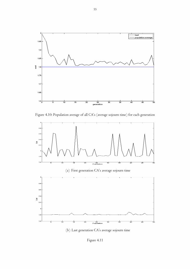
Figure 4.10: Population average of all CA’s (average sojourn time) for each generation

(a) First generation CA’s average sojourn time

(b) Last generation CA’s average sojourn time

Figure 4.11

55

Figure 4.12 shows the results for the heterogeneous service capacity case. For this illustrative example,

we set the mutation rate at 1%, the selection rate at 50%, and population size and number of

generations at 50. Here, we see that the GA brings the average cost from 1.72 to 1.65 at generation 6.

This is an improvement of 4% in just six generations which is quite significant in many systems. This

value is also quite close to the Nash value of 1.63 (approximately) as calculated using equation 8 for

heterogeneous service rate. In this case, the last generation average sojourn time value is approximately

at 1.64, hence yielding an optimal combination of behavioral parameters that is very close to the Nash

value of 1.63. The figure also shows the best CA in each generation. The following paragraphs explain

the sensitivity analysis performed on various GA parameters.

Figure 4.12: Population average of all CA’s (average sojourn time) for each generation

Table 4.4 shows results for the sensitivity analysis of the mutation rate i.e. the impact of the mutation

rate on the overall performance of the GA. The last two columns of the table are the average

performance across all CA’s for the initial population (IP) and the last generation (LG) respectively.

56

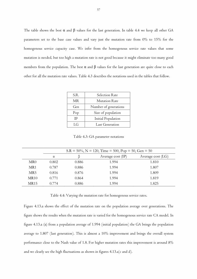
The table shows the best α and β values for the last generation. In table 4.4 we keep all other GA

parameters set to the base case values and vary just the mutation rate from 0% to 15% for the

homogenous service capacity case. We infer from the homogenous service rate values that some

mutation is needed, but too high a mutation rate is not good because it might eliminate too many good

members from the population. The best α and β values for the last generation are quite close to each

other for all the mutation rate values. Table 4.3 describes the notations used in the tables that follow.

S.R. Selection Rate

MR Mutation Rate

Gen Number of generations

Pop Size of population

IP Initial Population

LG Last Generation

Table 4.3: GA parameter notations

S.R = 50%, N = 120, Time = 500, Pop = 50, Gen = 50

α β Average cost (IP) Average cost (LG)

MR0 0.802 0.886 1.994 1.810

MR1 0.787 0.886 1.994 1.807

MR5 0.816 0.876 1.994 1.809

MR10 0.771 0.864 1.994 1.819

MR15 0.774 0.886 1.994 1.825

Table 4.4: Varying the mutation rate for homogenous service rates.

Figure 4.13.a shows the effect of the mutation rate on the population average over generations. The

figure shows the results when the mutation rate is varied for the homogenous service rate CA model. In

figure 4.13.a (a) from a population average of 1.994 (initial population) the GA brings the population

average to 1.807 (last generation). This is almost a 10% improvement and brings the overall system

performance close to the Nash value of 1.8. For higher mutation rates this improvement is around 8%

and we clearly see the high fluctuations as shown in figures 4.13.a(c and d).

57

0 5 10 15 20 25 30 35 40 45 501.8

1.82

1.84

1.86

1.88

1.9

1.92

1.94

1.96

1.98

2

generation

co

st

0 5 10 15 20 25 30 35 40 45 501.8

1.82

1.84

1.86

1.88

1.9

1.92

1.94

1.96

1.98

2

generation

co

st

(a) 1% MR (b) 5% MR

0 5 10 15 20 25 30 35 40 45 501.8

1.82

1.84

1.86

1.88

1.9

1.92

1.94

1.96

1.98

2

generation

co

st

0 5 10 15 20 25 30 35 40 45 501.8

1.82

1.84

1.86

1.88

1.9

1.92

1.94

1.96

1.98

2

generation

co

st

(c) 10% MR (d) 15% MR

Figure 4.13.a: Population average over generations while varying the mutation rate for homogenous service rates

Table 4.5 and figure 4.13.b show the heterogeneous service capacity case where all the GA parameters

are set to the base case values, and the mutation rate is varied between 0 and 15%. In this case we see

that the last generation average sojourn time (for all the CA’s) decreases for 1% mutation rate and then

observe a sharp increase for 5% mutation rate. We can also see that the best α value for the 5%

mutation rate is significantly different from the best α value for the other cases, indicating a local

optimum. For mutation rates of 10% and 15% we see that last generation average sojourn time

decreases compared to 5% mutation rate, but increases steadily compared to 1% mutation rate. In

figure 4.13.b (a) the population average decreases from 1.723 (initial population) to 1.638 (last

58

generation). This is a 5% improvement and it brings the overall system performance close to the Nash

value of 1.627. For the 5% MR, the performance is just improved by 0.9%.

S.R = 50%, N = 120, Time = 500, Pop = 50, Gen = 50

α β Average cost (IP) Average cost (LG)

MR0 0.664 0.930 1.723 1.639 MR1 0.744 0.924 1.723 1.638 MR5 0.347 0.756 1.723 1.708

MR10 0.742 0.470 1.723 1.643

MR15 0.992 0.997 1.723 1.660

Table 4.5: Varying the mutation rate for heterogeneous service rate.

0 5 10 15 20 25 30 35 40 45 501.6

1.62

1.64

1.66

1.68

1.7

1.72

1.74

generation

co

st

0 5 10 15 20 25 30 35 40 45 50

1.6

1.62

1.64

1.66

1.68

1.7

1.72

1.74

generation

co

st

(a) 1% MR (b) 5% MR

0 5 10 15 20 25 30 35 40 45 501.6

1.62

1.64

1.66

1.68

1.7

1.72

1.74

generation

co

st

0 5 10 15 20 25 30 35 40 45 50

1.6

1.62

1.64

1.66

1.68

1.7

1.72

1.74

generation

co

st

(c) 10% MR (d) 15% MR

Figure 4.13.b: Population average over generations while varying the mutation rate for heterogeneous

service rates

59

Table 4.6 shows the result when the selection rate is varied and all the other GA parameters are set to

the base case values except the mutation rate which is set to 1%. (i.e. less diversity in generations). In

the case of homogeneous service rates, selection rates of 25% and 60% resulted in higher average

sojourn times. For the 60% selection rate, the value of α is significantly different from the other values

in table 4.4, and this case has the highest average sojourn time. This might be a local optimum. Most of

the average sojourn time values for homogenous service rates are quite close to the Nash value (1.8).

For heterogeneous service rates, a very low selection rate of 25% gave slightly higher average sojourn

time values. The average sojourn time values are close to the Nash (1.627) in all the cases.

M.R = 1%, N = 120, Time = 500, Pop = 50, Gen = 50

Homogenous service rate Heterogeneous service rate

α β Average cost (IP)

Average cost (LG)

α β Average cost (IP)

Average cost (LG)

SR25 0.800 0.858 1.994 1.815 0.679 0.927 1.723 1.643

SR50 0.787 0.886 1.994 1.807 0.744 0.924 1.723 1.638

SR60 0.698 0.873 1.994 1.822 0.728 0.929 1.723 1.638

SR75 0.795 0.873 1.994 1.807 0.694 0.903 1.723 1.639

Table 4.6: Varying the selection rate

Table 4.7 portrays the results when the population size is varied, the mutation rate is kept at 1%, and

all other GA parameters are set to the base case values. From the table we see that there are only minor

variations in average sojourn time for homogenous service rates. The lowest value is when the

population size is 50, where the sojourn time (1.807) is very close to the Nash (1.8). For the

heterogeneous service rate we see that a population size of 100 results in the lowest average sojourn

time value of 1.628. It is to be noted that the best solution achieved in the last generation for both

homogenous service rate and heterogeneous service rate is very close to their respective Nash values.

60

M.R = 1%, S.R. = 50%, N = 120, Time = 500, Gen = 50

Homogenous service rate Heterogeneous service rate

α β Average cost (IP)

Average cost (LG)

α β Average cost (IP)

Average cost (LG)

P50 0.787 0.888 1.994 1.807 0.743 0.992 1.723 1.638

P100 0.749 0.849 2.031 1.813 0.986 0.996 1.728 1.628

P150 0.810 0.874 2.032 1.814 0.772 0.995 1.709 1.630

P200 0.777 0.851 2.011 1.815 0.917 0.981 1.701 1.635

Table 4.7: Varying the population size

CONCLUSIONS

In this paper we show how by using a genetic algorithm we model the evolution of customers as they

experience the consequences of queuing. The GA model we present in this paper looks into collective

learning i.e. it optimizes the overall welfare of the system rather than the individual performance. Using

a genetic algorithm we modeled customers who optimize their behavior through learning from their

past experiences and information at their disposal. This paper is a step further in the design of

intelligent decision makers. In the previous paper, i.e. the CA model, we assumed that the behavioral

parameters (α and β) in the adaptive expectations based rule are given and fixed for a given simulation

run. By using a GA, we improved the CA model by enabling the group of agents to change their

behavioral parameters based on their experiences.

We illustrated how the genetic algorithm minimizes the average sojourn time of the system within a

few generations. In the previous paper we showed the influence of α and β on the sojourn time. We

concluded that slower updating of the expectations based on the agents’ own experience results in a

better overall performance of the CA. The GA results corroborated the findings of the CA model.

We also conducted sensitivity analysis to show the effects of the GA parameters on the optimization

process. We found that the mutation rate has a significant influence on the optimization process. For

both the homogenous and heterogeneous case a 1% mutation rate gave the best results. A 5% mutation

61

rate gave the worst average sojourn time value of 1.708 for the heterogeneous service capacity. We also

illustrated the influence of selection rate and size of population. Varying the population size did not

have a significant influence on the results. The selection rate did not have a significant influence in the

case of heterogeneous service rates, while 60% selection rate gave a relatively higher average sojourn

time value (1.822) for the homogenous case

Concerning the GA, we are interested in investigating the use of different techniques in each phase. For

example using weighted pairing instead of random pairing. In weighted pairing, the population member

with the lowest cost has the greatest probability of mating than the population member with the

highest cost. Another interesting approach would be a comparative analysis of other heuristics such as

swarm intelligence, ant colony optimization, simulated annealing etc. along with GA’s to see the

effectiveness of these techniques for the problem we are concerned with.

62

4.3 A TALE OF THREE RESTAURANTS: AN EXPERIMENTAL APPROACH

TO UNDERSTANDING DECISION MAKING IN QUEUEING SYSTEMS

(with Carlos Delgado, Ann van Ackere and Erik R. Larsen)

ABSTRACT

In this paper we show how through a simple experimental setup, we can study decision making in a

multi-channel service facility. The agent based framework described in the first paper is used to design

this experimental study. We show how the experiment was set up to collect data from human subjects

who take the role of a virtual agent. This experimental data helps us to validate the proposed agent

based framework, to compare decision making strategies, and analyze the effects of behavioral

parameters on decision making.

INTRODUCTION

We humans are important entities; we design the systems around us and influence their functioning.

Behavioral operations analyze the behavior of human beings in complex decision problems. Most of the

analytical and simulation models in operations consider these human agents to be rational, but the fact

is human beings are not rational. Understanding human behavior and the role of cognition in complex

human behavior has recently received attention in economics, finance, marketing, etc., but is largely

absent in the field of operations. Gino and Pisano (2008) argue that operations management (OM)

should also follow this approach and incorporate behavioral and cognitive factors into OM models.

Economists for a long time assumed people to be rational and built their models based on this

assumption. In reality people have limited capability to process information and they follow rules of

thumb in their decision making, i.e. humans are boundedly rational (Gino and Pisano, 2008).

Economic models these days have moved away from the assumption that human beings are rational,

and try to explain and predict behavior. This has also trickled into the fields of finance and marketing.

63

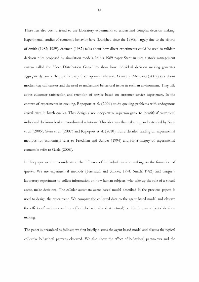
There has also been a trend to use laboratory experiments to understand complex decision making.

Experimental studies of economic behavior have flourished since the 1980s’, largely due to the efforts

of Smith (1982; 1989). Sterman (1987) talks about how direct experiments could be used to validate

decision rules proposed by simulation models. In his 1989 paper Sterman uses a stock management

system called the “Beer Distribution Game” to show how individual decision making generates

aggregate dynamics that are far away from optimal behavior. Aksin and Mehrotra (2007) talk about

modern day call centers and the need to understand behavioral issues in such an environment. They talk

about customer satisfaction and retention of service based on customer service experiences. In the

context of experiments in queuing, Rapoport et al. (2004) study queuing problems with endogenous

arrival rates in batch queues. They design a non-cooperative n-person game to identify if customers’

individual decisions lead to coordinated solutions. This idea was then taken up and extended by Seale

et al. (2005), Stein et al. (2007) and Rapoport et al. (2010). For a detailed reading on experimental

methods for economists refer to Friedman and Sunder (1994) and for a history of experimental

economics refer to Guala (2008).

In this paper we aim to understand the influence of individual decision making on the formation of

queues. We use experimental methods (Friedman and Sunder, 1994; Smith, 1982) and design a

laboratory experiment to collect information on how human subjects, who take up the role of a virtual

agent, make decisions. The cellular automata agent based model described in the previous papers is

used to design the experiment. We compare the collected data to the agent based model and observe

the effects of various conditions (both behavioral and structural) on the human subjects’ decision

making.

The paper is organized as follows: we first briefly discuss the agent based model and discuss the typical

collective behavioral patterns observed. We also show the effect of behavioral parameters and the

64

Age

nt

n+1

Age

nt

n+2

Age

nt

n+

3

Age

nt

n+4

Age

nt

n

Age

nt

n-1

Age

nt

n-2

Age

nt

n-3

……..

……..

…

….. ……..

……..

……..

……..

……..

influence of initial conditions on the collective behavioral patterns. Finally, we present the experimental

design and discuss the observations made based on the results of the experiments.

THE AGENT BASED QUEUING MODEL

In this section, we very briefly describe the agent based queuing model as proposed in the previous

papers. We consider a group of customers who choose a service facility each time period based on their

expectation of sojourn time at each facility. A one dimensional cellular automata (Gutowitz, 1991;

Wolfram, 1984) is used to model such a system.

The model assumes a ring structure, as shown in figure 4.14. Each cell of the CA (cellular automata) is

an agent who has two neighbors, one on each side. The parameter ‘K’ in the model defines the

neighborhood (Lomi et al., 2003) i.e. the number of neighbors on each side from whom the agent gets

local information (van Ackere and Larsen, 2004). The neighborhood in real life could be considered as

a social network consisting of friends, colleagues, next door neighbors etc. or any physical network.

Figure 4.14: Structure of cellular automata agent based queuing model

Refer to section 4.1 for a detailed description of the agent based framework used for the experimental

study.

65

Simulation setup for the agent based model

The CA model consists of 120 agents and 3 service facilities. In this study we fix the neighborhood size

at K = 1 i.e. two neighbors for each agent, one on each side. We experiment with both homogeneous

and heterogeneous service rates. In one set of simulations we use identical service rates for all three

facilities (µ = 5; 5 agents per unit of time) and in the other we use 3, 5 and 7 as service rates for

facilities 1, 2 and 3 respectively. We also experiment with different values for the behavioral parameters

α and β. To explain the observed collective behavior, we show the case where the agents use the same

behavioral parameters value of α = β = 0.1. Finally, the model is simulated for 60 time periods. This is

sufficient to observe the evolution of the automata and for the model to reach steady state, i.e. the

collective behavior remains the same for longer simulations. Each agent is allocated an initial value for

the memory of the expected sojourn times for each facility. These values are distributed randomly

around the lowest achievable average sojourn time.

Nash equilibrium

Given that the three facilities are identical (µ = 5), the Nash equilibrium corresponds to the case where

agents are equally distributed, 40 choosing each of the three facilities. This results in a sojourn time

value of 5.4 time units. For variable service capacity with the values µ = 3, 5, and 7 the Nash

equilibrium results in a sojourn time value of 4.88 time units.

Simulation results

Figures 4.15 and 4.16 portray the collective behaviors and the aggregate results (average sojourn time)

that are observed when simulating the agent based queuing model. Figures 4.15 (a, b, c) and 4.16 (a, b,

c) are for homogenous service rates (i.e. µ = 5 for all service facilities) and figures 4.15 (d, e, f) and

4.16 (d, e, f) are for heterogeneous service rates of 3, 5, and 7 agents per unit of time for facilities 1, 2

and 3 respectively.

66

Figure 4.15 shows the spatial-temporal evolution of the choice of service facility over 60 time periods.

The figure illustrates the case where the behavioral parameters are α = β = 0.1 i.e. the agents update

their expectations fast, relying more on recent experiences. In each sub-figure, the x-axis represents the

simulation time and the y-axis the 120 agents. The colors in the figure indicates the facility chosen by

each agent each time period. The color code is as follows: black = facility 1, grey = facility 2 and white

= facility 3.

We observe that there is always an initial learning phase whose length can vary. During this phase

agents learn about the system by exploring various facilities. For example, in figure 4.15 (a), the

learning phase is 8 time periods after which we observe a pattern emerging. For instance, agent 1 in

figure 4.15 (a) tries the facilities in the following sequence 21323132 and then settles in facility 1

(black). This observed behavior is highly dependent on the initial allocated expected sojourn time

values. This learning phase also results in high average sojourn time value as seen in figure 4.16 (a), the

average sojourn time peaks at 15 time units at time period 8. The average sojourn time is high due to

the fact that agents are trying out various facilities. This results in significantly more than 40 agents

showing up at the same facility at a given period, and thus resulting in congestion at that facility. After

this learning phase we see patterns emerging as illustrated in figure 4.15.

In figure 4.15 we present three typical collective behaviors observed for homogenous and

heterogeneous service rates. The three behaviors are the following: (i) a stable pattern after the learning

phase as seen in figures 4.15 (a) and 4.15 (d), (ii) a few agents are still switching facilities and not

settling down as shown in figures 4.15 (b) and 4.15 (e) and (iii) a facility is forgotten as in figures 4.15

(c) and 4.15 (f).

67

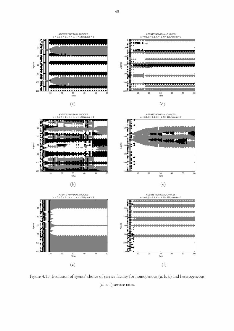
AGENTS´INDIVIDUAL CHOICES

= 0.1, = 0.1, K = 1, N = 120,Nqueue = 3

Time

Agents

10 20 30 40 50 60

20

40

60

80

100

120

AGENTS´INDIVIDUAL CHOICES

= 0.1, = 0.1, K = 1, N = 120,Nqueue = 3

Time

Agents

10 20 30 40 50 60

20

40

60

80

100

120

(a) (d)

AGENTS´INDIVIDUAL CHOICES

= 0.1, = 0.1, K = 1, N = 120,Nqueue = 3

Time

Agents

10 20 30 40 50 60

20

40

60

80

100

120

AGENTS´INDIVIDUAL CHOICES

= 0.1, = 0.1, K = 1, N = 120,Nqueue = 3

Time

Agents

10 20 30 40 50 60

20

40

60

80

100

120

(b) (e)

AGENTS´INDIVIDUAL CHOICES

= 0.1, = 0.1, K = 1, N = 120,Nqueue = 3

Time

Agents

10 20 30 40 50 60

20

40

60

80

100

120

AGENTS´INDIVIDUAL CHOICES

= 0.1, = 0.1, K = 1, N = 120,Nqueue = 3

Time

Agents

10 20 30 40 50 60

20

40

60

80

100

120

(c) (f)

Figure 4.15: Evolution of agents’ choice of service facility for homogenous (a, b, c) and heterogeneous

(d, e, f) service rates.

68

(a) (d)

(b) (e)

(c) (f)

Figure 4.16: Average sojourn time with minimum and maximum value

69

In figures 4.15 (a) and 4.15 (d), as explained above, after the learning phase a stable pattern emerges.

During the learning phase we see that the average sojourn time fluctuates heavily. From figure 4.16 (a),

we see that the maximum sojourn time goes up to 15 time units, which is almost three times the Nash

value (5.4). In figure 4.16 (d), we observe the same: at time period 3 it peaks at 15.58 which is again

more than three times the Nash value (4.88). After this phase, the system reaches a kind of steady state

and the average sojourn time stabilizes around 5.46 (for 4.15 (a)) and 4.96 (for 4.15 (d)) respectively;

these values are very close to the social optimum and Nash value. The slight fluctuation we see in

sojourn time values are due to a few agents switching facilities.

Figures 4.15 (b) and 4.15 (e) show the case where a few agents do not settle down and keep trying

different facilities. We refer to this behavior as non-stable because we do not observe a stable pattern

even if we run the simulation for a longer time. This is evident from the sojourn time graphs of figures

4.16 (b) and 4.16 (e) where the average sojourn time keeps fluctuating. The average sojourn time values

at steady state for 4.15 (b) and 4.15 (e) are 6.11 and 5.00 respectively.

Finally, figures 4.15 (c) and 4.15 (f) portray the case when one facility is forgotten. In the example

shown, facility 1 (black) is forgotten. Note that for the heterogeneous case the black facility has the

lowest service rate of 3 agents per unit of time. The reasoning why a facility is forgotten is what we call

a reputation effect due to information diffusion. For example, in figure 4.15 (c), at time period 5, 114

agents show up at facility 1. This results in a high average sojourn time value for that facility, hence a

bad reputation. Due to local interactions this information diffuses among the agents resulting in facility

1 being avoided for periods 6 and 7 respectively. Finally, we see at period 9, facility 1 being used by all

the 120 agents causing congestion at the facility and eventually forgotten completely. Note we use low

behavioral parameter value (α = β = 0.1) in this example i.e. agents update their expectations relying

heavily on recent experience.

70

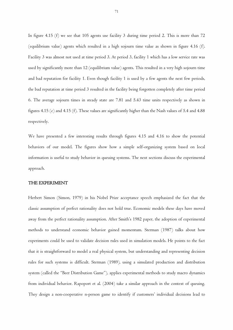
In figure 4.15 (f) we see that 105 agents use facility 3 during time period 2. This is more than 72

(equilibrium value) agents which resulted in a high sojourn time value as shown in figure 4.16 (f).

Facility 3 was almost not used at time period 3. At period 3, facility 1 which has a low service rate was

used by significantly more than 12 (equilibrium value) agents. This resulted in a very high sojourn time

and bad reputation for facility 1. Even though facility 1 is used by a few agents the next few periods,

the bad reputation at time period 3 resulted in the facility being forgotten completely after time period

6. The average sojourn times in steady state are 7.81 and 5.43 time units respectively as shown in

figures 4.15 (c) and 4.15 (f). These values are significantly higher than the Nash values of 5.4 and 4.88

respectively.

We have presented a few interesting results through figures 4.15 and 4.16 to show the potential

behaviors of our model. The figures show how a simple self-organizing system based on local

information is useful to study behavior in queuing systems. The next sections discuss the experimental

approach.

THE EXPERIMENT

Herbert Simon (Simon, 1979) in his Nobel Prize acceptance speech emphasized the fact that the

classic assumption of perfect rationality does not hold true. Economic models these days have moved

away from the perfect rationality assumption. After Smith’s 1982 paper, the adoption of experimental

methods to understand economic behavior gained momentum. Sterman (1987) talks about how

experiments could be used to validate decision rules used in simulation models. He points to the fact

that it is straightforward to model a real physical system, but understanding and representing decision

rules for such systems is difficult. Sterman (1989), using a simulated production and distribution

system (called the “Beer Distribution Game”), applies experimental methods to study macro dynamics

from individual behavior. Rapoport et al. (2004) take a similar approach in the context of queuing.

They design a non-cooperative n-person game to identify if customers’ individual decisions lead to

71

coordinated solutions. This again looks into individual behavior and how it influences and leads to

macro dynamics.

We adopt a similar approach to that of Sterman and Rapoport. The behavioral queuing model as

described in the previous section is used to design a laboratory experiment (Friedman and Sunder,

1994). In the simulation model, we used an adaptive expectation based decision rule. We showed

through figures 4.10 and 4.11 how different collective behaviors could be observed. Individual decision

making and its influence on the systems performance (i.e. average sojourn time of the system) was

illustrated. The aim of this experimental approach is to collect experimental data to validate the

decision rule as described previously. We try to answer the following questions through this

experimental approach:

1) How do customers adapt based on system behavior?

This is an interesting question because it will help us to see how customers learn from the system that

serves them, and how they use this information (i.e. regarding the state of the system) to their benefit.

2) How does an individual customer influence the performance of the system?

We would like to see how an individual human subject influences the entire system for good or bad,

which in turn gives an idea regarding information diffusion.

3) Do we see the same behavior as we observed in the simulated model?

This question will help us validate our agent based framework. Through the simulation model we

showed three common collective behaviors. We would like to see how the model behaves when a

virtual agent is replaced by a human subject (instead of 120 virtual agents we will have a human subject

and 119 virtual agents).

4) What decision making strategy does the human subject adopt?

72

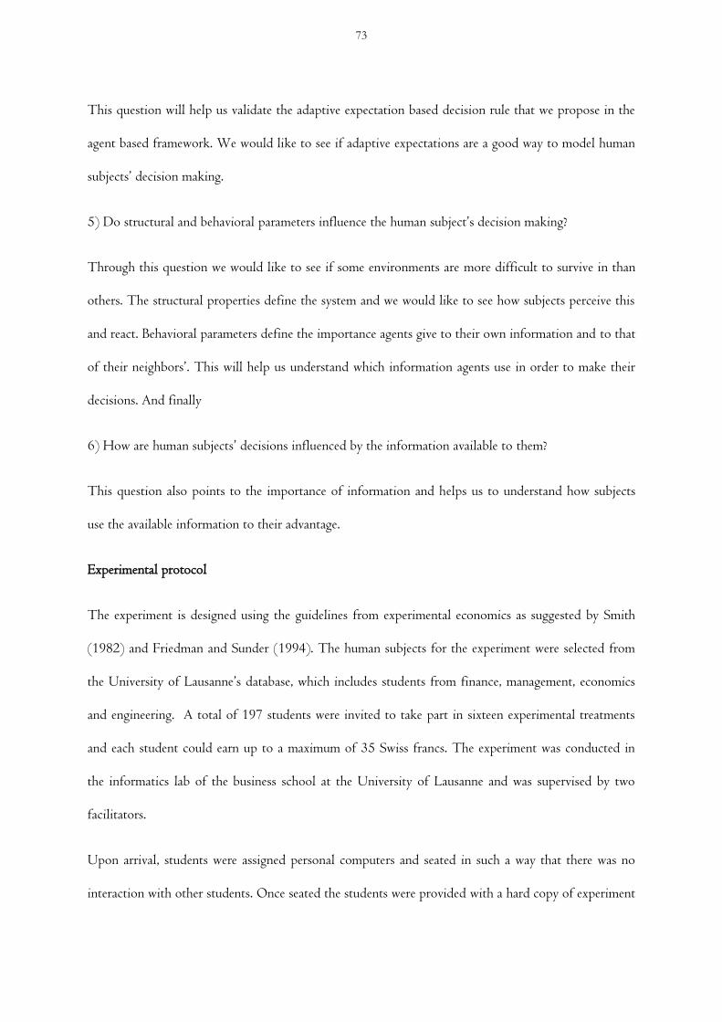
This question will help us validate the adaptive expectation based decision rule that we propose in the

agent based framework. We would like to see if adaptive expectations are a good way to model human

subjects’ decision making.

5) Do structural and behavioral parameters influence the human subject’s decision making?

Through this question we would like to see if some environments are more difficult to survive in than

others. The structural properties define the system and we would like to see how subjects perceive this

and react. Behavioral parameters define the importance agents give to their own information and to that

of their neighbors’. This will help us understand which information agents use in order to make their

decisions. And finally

6) How are human subjects’ decisions influenced by the information available to them?

This question also points to the importance of information and helps us to understand how subjects

use the available information to their advantage.

Experimental protocol

The experiment is designed using the guidelines from experimental economics as suggested by Smith

(1982) and Friedman and Sunder (1994). The human subjects for the experiment were selected from

the University of Lausanne’s database, which includes students from finance, management, economics

and engineering. A total of 197 students were invited to take part in sixteen experimental treatments

and each student could earn up to a maximum of 35 Swiss francs. The experiment was conducted in

the informatics lab of the business school at the University of Lausanne and was supervised by two

facilitators.

Upon arrival, students were assigned personal computers and seated in such a way that there was no

interaction with other students. Once seated the students were provided with a hard copy of experiment

73

instructions and a consent form, which should be signed before starting the experiment. A short

introduction regarding the computer interface and the task was given.

The experiment has been designed to study how customers choose a service facility (restaurants in our

case) based on their experiences. The task for each subject is to make one decision each time period, i.e.

choice of restaurant, and provide estimates of the waiting time (sojourn time) he/she would expect at

each of the restaurants. At the start of the experiment initial estimates for each restaurant were

provided. For the subsequent time periods subjects were provided with information regarding sojourn

time at their chosen restaurant, their previous day’s expectations for the restaurants and the best

performing virtual neighbors’ chosen restaurant and sojourn time. The subjects were asked to enter the

following information using the interface each experimental time period: 1) choice of restaurant and 2)

their expectations for the three restaurants. The interface and instructions used in the experiment are

provided in the appendix of this paper.

The reward for the subjects was based on their performance. Performance is measured based on their

cumulative sojourn time achieved at the end of the experiment. Minimizing the cumulative sojourn

time was the goal for the subjects. The subjects made decisions for 60 experimental periods and on an

average completed the experiment in 60 minutes.

Treatments

The treatments explore the following:

1) Compare the behavioral patterns observed during simulation with that of the experimental

results.

2) The influence of structural properties of the system on subjects’ decision making i.e.

homogenous and heterogeneous service capacities.

3) Finally, the effect of behavioral parameters α and β on subjects decision making.

74

The following paragraphs explain what the treatments are.

Recall that in figure 4.15 we show three system level collective patterns that we observe while

simulating. We have three treatments based on the observed collective behavior.

(1) Stable pattern after the initial learning phase (naming convention S)

(2) Non-stable pattern where the system does not settle down (naming convention NS), and

(3) Stable pattern with a forgotten facility (naming convention F).

In order to explore the effect of behavioral parameters we use the following three parameter values for

our treatments:

(1) α, β = 0.1 i.e. agents update their expectations fast, relying more on recent experience (naming

convention 1). (2) α, β = 0.5 i.e. agents give equal weight to past expectations and recent experiences

(naming convention 5), and (3) α, β = 0.9 i.e. inertia to recent experiences, relying more on past

expectations (naming convention 9).

Each system level collective pattern treatment can thus take one behavioral parameter value. We have

nine treatments if we combine the collective pattern with that of the behavioral parameter values. We

could not observe forgotten collective behavior with behavioral parameter value 0.9, hence we exclude

this combination. We thus have eight treatments.

Finally, we would like to understand the influence of structural properties of the system on subjects’

decision making. Hence we have homogenous service capacity and heterogeneous capacity treatments.

For each of these treatments we have eight treatments as previously described, resulting in a total of 16

treatments. We refer to the homogenous service capacity treatments as group E treatments and

heterogeneous capacity treatments as group D treatments. Tables 4.8, 4.9 and 4.10 summarize the

condition for each treatment.

75

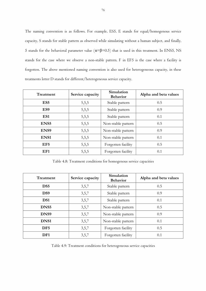
The naming convention is as follows. For example, ES5, E stands for equal/homogenous service

capacity, S stands for stable pattern as observed while simulating without a human subject, and finally,

5 stands for the behavioral parameter value (α=β=0.5) that is used in this treatment. In ENS5, NS

stands for the case where we observe a non-stable pattern. F in EF5 is the case where a facility is

forgotten. The above mentioned naming convention is also used for heterogeneous capacity, in these

treatments letter D stands for different/heterogeneous service capacity.

Treatment Service capacity Simulation Behavior

Alpha and beta values

ES5 5,5,5 Stable pattern 0.5

ES9 5,5,5 Stable pattern 0.9

ES1 5,5,5 Stable pattern 0.1

ENS5 5,5,5 Non-stable pattern 0.5

ENS9 5,5,5 Non-stable pattern 0.9

ENS1 5,5,5 Non-stable pattern 0.1

EF5 5,5,5 Forgotten facility 0.5

EF1 5,5,5 Forgotten facility 0.1

Table 4.8: Treatment conditions for homogenous service capacities

Treatment Service capacity Simulation Behavior

Alpha and beta values

DS5 3,5,7 Stable pattern 0.5

DS9 3,5,7 Stable pattern 0.9

DS1 3,5,7 Stable pattern 0.1

DNS5 3,5,7 Non-stable pattern 0.5

DNS9 3,5,7 Non-stable pattern 0.9

DNS1 3,5,7 Non-stable pattern 0.1

DF5 3,5,7 Forgotten facility 0.5

DF1 3,5,7 Forgotten facility 0.1

Table 4.9: Treatment conditions for heterogeneous service capacities

76

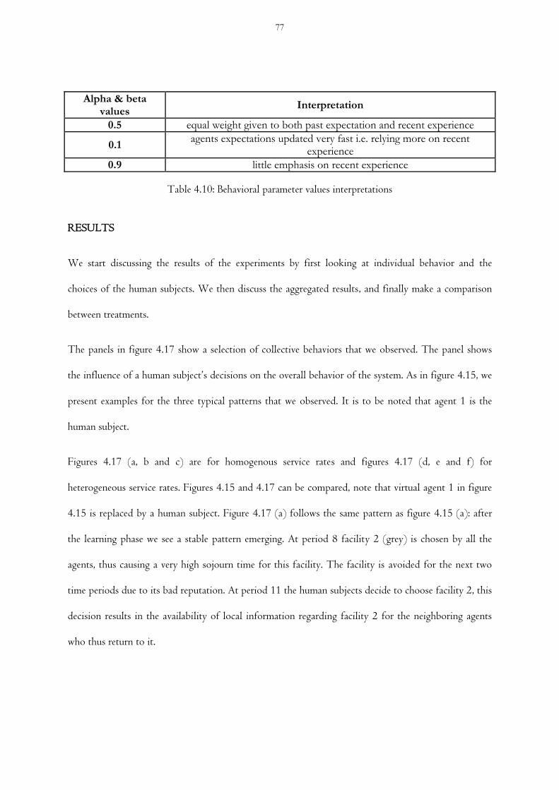
Alpha & beta values

Interpretation

0.5 equal weight given to both past expectation and recent experience

0.1 agents expectations updated very fast i.e. relying more on recent

experience

0.9 little emphasis on recent experience

Table 4.10: Behavioral parameter values interpretations

RESULTS

We start discussing the results of the experiments by first looking at individual behavior and the

choices of the human subjects. We then discuss the aggregated results, and finally make a comparison

between treatments.

The panels in figure 4.17 show a selection of collective behaviors that we observed. The panel shows

the influence of a human subject’s decisions on the overall behavior of the system. As in figure 4.15, we

present examples for the three typical patterns that we observed. It is to be noted that agent 1 is the

human subject.

Figures 4.17 (a, b and c) are for homogenous service rates and figures 4.17 (d, e and f) for

heterogeneous service rates. Figures 4.15 and 4.17 can be compared, note that virtual agent 1 in figure

4.15 is replaced by a human subject. Figure 4.17 (a) follows the same pattern as figure 4.15 (a): after

the learning phase we see a stable pattern emerging. At period 8 facility 2 (grey) is chosen by all the

agents, thus causing a very high sojourn time for this facility. The facility is avoided for the next two

time periods due to its bad reputation. At period 11 the human subjects decide to choose facility 2, this

decision results in the availability of local information regarding facility 2 for the neighboring agents

who thus return to it.

77

AGENTS´INDIVIDUAL CHOICES

= 0.1, = 0.1, K = 1, N = 120,Nqueue = 3

Time

Agents

10 20 30 40 50 60

20

40

60

80

100

120

AGENTS´INDIVIDUAL CHOICES

= 0.1, = 0.1, K = 1, N = 120,Nqueue = 3

Time

Agents

10 20 30 40 50 60

20

40

60

80

100

120

(a) ES1 subject 8 (d) DS1 subject 3

AGENTS´INDIVIDUAL CHOICES

= 0.1, = 0.1, K = 1, N = 120,Nqueue = 3

Time

Agents

10 20 30 40 50 60

20

40

60

80

100

120

AGENTS´INDIVIDUAL CHOICES

= 0.1, = 0.1, K = 1, N = 120,Nqueue = 3

Time

Agents

10 20 30 40 50 60

20

40

60

80

100

120

(b) ENS1 subject 11 (e) DNS1 subject 10

AGENTS´INDIVIDUAL CHOICES

= 0.1, = 0.1, K = 1, N = 120,Nqueue = 3

Time

Agents

10 20 30 40 50 60

20

40

60

80

100

120

AGENTS´INDIVIDUAL CHOICES

= 0.1, = 0.1, K = 1, N = 120,Nqueue = 3

Time

Agents

10 20 30 40 50 60

20

40

60

80

100

120

(c) EF1 subject 2 (f) DF1 subject 8

Figure 4.17: Evolution of players choice of service facility for homogenous (a, b, c) and heterogeneous

(d, e, f) service rates.

78

Another interesting result is observed in figure 4.17 (d). Comparing the simulation result as illustrated

in figure 4.15 (d), we expected just a stable collective pattern. What we see is that facility 1 is forgotten

in figure 4.17 (d). Facility 1 is the one with the lowest service capacity (µ=3) hence, if too many agents

use this facility it will result in a high sojourn time. We see from figure 4.17 (d) that the human subject

used facility 1 only once, during the entire 60 days experimental period i.e. at period 3. After period

28, due to congestion at facility 1, the virtual agents decide to abandon this facility. At period 32 all

the agents and the human subject throng facility 3, resulting in a very high sojourn time. The decision

of all the agents to use facility 3 (resulting in extremely high sojourn time) at period 32 brought back

facility 1 at period 33. The fact that facility 1 has the lowest service capacity, and 35 agents (optimal

value =12) used this facility implies that at period 34 facility 1 is permanently forgotten due to the

past experiences.

In figure 4.17 (c) at period 7 all the agents choose facility 3 resulting in a very high sojourn time. This

bad experience resulted in the facility being avoided by the 119 virtual agents at period 8. But because

the human subject decided to choose facility 3 in period 8, it was not forgotten. We see the same

behavior in figures 4.17 (e) in period 14, and 4.17 (f) in period 11 where the human subjects’ decision

to use facility 1 made the information regarding facility 1 available to the virtual agents.

Figures 4.18 and 4.19 portray individual decision making for group E and group D treatments. Recall

that we refer to homogenous service capacity treatments as group E treatments and heterogeneous

service capacity treatments as group D treatments. In these figures we compare virtual agent 1’s (of the

simulation) decision making with that of the human subject (who takes the role of the virtual agent 1

in the experiment). Note that we present selective results to highlight human subjects’ decision making,

and the influence of their decisions on the overall system performance.

79

(a) (d)

(b) (e)

(c) (f)

Figure 4.18: Individual decision making for homogenous service capacity treatments virtual agent (a, b,

c) vs human subject (d, e,f).

80

(a) (d)

(b) (e)

(c) (f)

Figure 4.19: Individual decision making for heterogenous service capacity treatments virtual agent (a, b,

c) vs human subject (d, e,f).

A first glance at figures 4.18 and 4.19 shows how a human subject introduces variability into the

system. Even though subjects might be following a particular strategy and be better off at that, subjects

sometimes choose randomly. The influence of the human subjects’ decisions’ on the overall collective

behavior was explained in the previous sections and shown in figure 4.17. In figure 4.18 (d) we see that

81

subject 8 chose the same facility as the virtual agent for the first three periods. Subject 8 uses facility 2

most of the time except for 7 time periods where she tries out facilities 1 and 3. Subject 8’s average

sojourn time (4.6) i.e. her performance was much better than the overall system performance (6.63),

simulated system performance (6.35) and the Nash equilibrium value (5.4). Subject 11 of treatment

ENS1 showed switching behavior. This subject’s performance (5.66) was slightly better than the

overall system (6.06) but higher than the Nash equilibrium value (5.4). Finally, subject 2 of treatment

EF1 chooses facility 2 until period 6, facility 3 from period 7 until 12 and facility 1 from 13 to 24.

She then moves back to facility 2, but after period 38 she switches between the facilities.

In figure 4.19 (d) subject 3 of DS1 treatment sticks mostly to facility 2 from period 11 to 31, similar

to virtual agent 1 of the simulation. The subject then switches between facilities 2 and 3, neglecting

facility 1. Note that facility 1 has the lowest service capacity (3) hence subject 3 did not find it

appealing. Subject 10 of treatment DNS1 in figure 4.19 (e) uses facility 1 most of the time. Even

though facility 1 has the lowest service capacity, this subject chose facility 1 and performed well. The

subject performed (4.83) well below the overall system performance (5.4) and a little below the Nash

equilibrium value (4.88). Finally, subject 8 of treatment DF1 switches between the facilities and does

not settle down.

Tables 4.12 and 4.13 give an overview of the total number of subjects in each treatment and the

observed collective behavior. The tables also compare the performance of the system for simulated and

experimental results. As explained in the agent based queuing model section, simulating the model we

observed three distinct system level collective patterns: Pattern ‘S’ wherein the agents follow a kind of

stable pattern after the learning phase; pattern ‘C’ where the agents do not stabilize /settle down and

finally pattern ‘F’ where a facility is forgotten. Table 4.11 defines the variables that are used in tables

4.12 and 4.13 respectively.

82

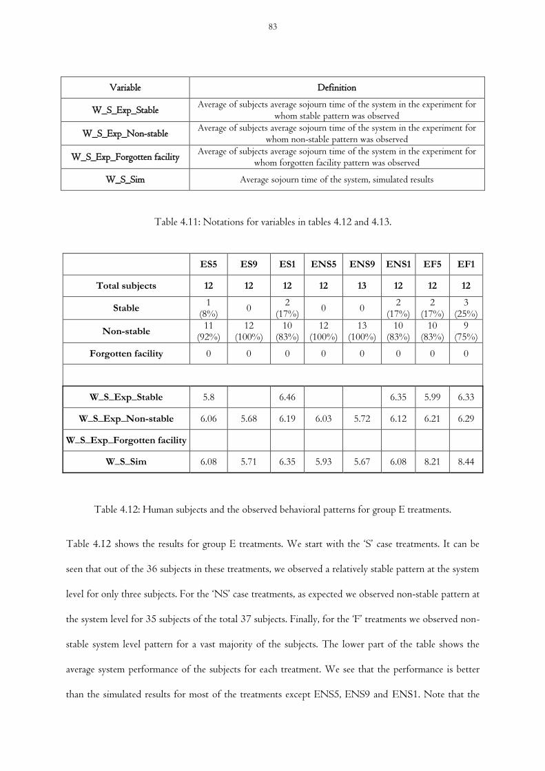
Variable Definition

W_S_Exp_Stable Average of subjects average sojourn time of the system in the experiment for

whom stable pattern was observed

W_S_Exp_Non-stable Average of subjects average sojourn time of the system in the experiment for

whom non-stable pattern was observed

W_S_Exp_Forgotten facility Average of subjects average sojourn time of the system in the experiment for

whom forgotten facility pattern was observed

W_S_Sim Average sojourn time of the system, simulated results

Table 4.11: Notations for variables in tables 4.12 and 4.13.

ES5 ES9 ES1 ENS5 ENS9 ENS1 EF5 EF1

Total subjects 12 12 12 12 13 12 12 12

Stable 1

(8%) 0

2 (17%)

0 0 2

(17%) 2

(17%) 3

(25%)

Non-stable 11

(92%) 12

(100%) 10

(83%) 12

(100%) 13

(100%) 10

(83%) 10

(83%) 9

(75%)

Forgotten facility 0 0 0 0 0 0 0 0

W_S_Exp_Stable 5.8 6.46 6.35 5.99 6.33

W_S_Exp_Non-stable 6.06 5.68 6.19 6.03 5.72 6.12 6.21 6.29

W_S_Exp_Forgotten facility

W_S_Sim 6.08 5.71 6.35 5.93 5.67 6.08 8.21 8.44

Table 4.12: Human subjects and the observed behavioral patterns for group E treatments.

Table 4.12 shows the results for group E treatments. We start with the ‘S’ case treatments. It can be

seen that out of the 36 subjects in these treatments, we observed a relatively stable pattern at the system

level for only three subjects. For the ‘NS’ case treatments, as expected we observed non-stable pattern at

the system level for 35 subjects of the total 37 subjects. Finally, for the ‘F’ treatments we observed non-

stable system level pattern for a vast majority of the subjects. The lower part of the table shows the

average system performance of the subjects for each treatment. We see that the performance is better

than the simulated results for most of the treatments except ENS5, ENS9 and ENS1. Note that the

83

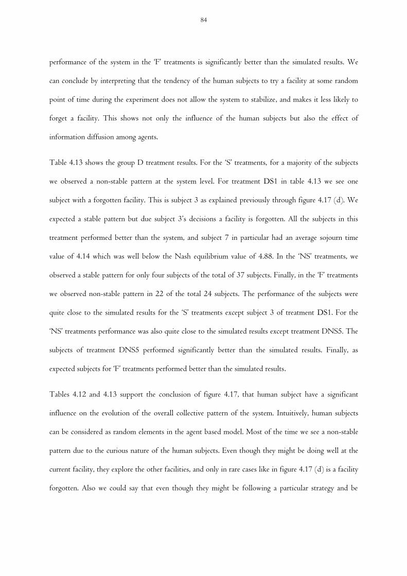
performance of the system in the ‘F’ treatments is significantly better than the simulated results. We

can conclude by interpreting that the tendency of the human subjects to try a facility at some random

point of time during the experiment does not allow the system to stabilize, and makes it less likely to

forget a facility. This shows not only the influence of the human subjects but also the effect of

information diffusion among agents.

Table 4.13 shows the group D treatment results. For the ‘S’ treatments, for a majority of the subjects

we observed a non-stable pattern at the system level. For treatment DS1 in table 4.13 we see one

subject with a forgotten facility. This is subject 3 as explained previously through figure 4.17 (d). We

expected a stable pattern but due subject 3’s decisions a facility is forgotten. All the subjects in this

treatment performed better than the system, and subject 7 in particular had an average sojourn time

value of 4.14 which was well below the Nash equilibrium value of 4.88. In the ‘NS’ treatments, we

observed a stable pattern for only four subjects of the total of 37 subjects. Finally, in the ‘F’ treatments

we observed non-stable pattern in 22 of the total 24 subjects. The performance of the subjects were

quite close to the simulated results for the ‘S’ treatments except subject 3 of treatment DS1. For the

‘NS’ treatments performance was also quite close to the simulated results except treatment DNS5. The

subjects of treatment DNS5 performed significantly better than the simulated results. Finally, as

expected subjects for ‘F’ treatments performed better than the simulated results.

Tables 4.12 and 4.13 support the conclusion of figure 4.17, that human subject have a significant

influence on the evolution of the overall collective pattern of the system. Intuitively, human subjects

can be considered as random elements in the agent based model. Most of the time we see a non-stable

pattern due to the curious nature of the human subjects. Even though they might be doing well at the

current facility, they explore the other facilities, and only in rare cases like in figure 4.17 (d) is a facility

forgotten. Also we could say that even though they might be following a particular strategy and be

84

better off at that, subjects sometimes choose randomly (later on we will discuss this randomness the

subjects introduce).

Through subject 8 of treatment ES1 i.e. figure 4.17 (a), we show how information diffuses. Facility 2

was forgotten after period 8, but because the human subject chose the facility in period 11, new

information regarding facility 2 was available for the other agents. Summarizing, the above sections

show the influence of a human agent on the systems’ overall performance (i.e. how a single subject can

influence the macro behavior), and how information diffuses among agents in a simple agent based

queuing model with local interactions.

DS5 DS9 DS1 DNS5 DNS9 DNS1 DF5 DF1

Total subjects 13 13 13 13 12 12 12 12

Stable 0 0 1

(8%) 1

(8%) 0

3 (25%)

0 2

(17%)

Non-stable 13

(100%) 13

(100%) 11

(85%) 12

(92%) 12

(100%) 9

(75%) 12

(100%) 10

(83%)

Forgotten facility 0 0 1

(8%) 0 0 0 0 0

W_S_Exp_Stable 5.2 5.07 5.3 5.42

W_S_Exp_Non-stable 5.08 5.02 5.32 5.09 5.08 5.33 5.24 5.43

W_S_Exp_Forgotten facility 5.61

W_S_Sim 5.06 5.04 5.26 5.28 4.98 5.42 5.58 5.64

Table 4.13: Human subjects and the observed behavioral patterns for group D treatments.

We now turn to the aggregated results of the treatments. In figures 4.20 (a) and 4.21 (a) we compare

the average sojourn time of the system (experimental and simulated) with the equilibrium values for

homogenous and heterogeneous service capacity treatment groups. Figures 4.20 (b) and 4.21 (b)

compare the average of the subjects’ sojourn time (experimental), the average of the corresponding

virtual agents’ sojourn time in the simulation, and the equilibrium values for group E and D treatments.

85

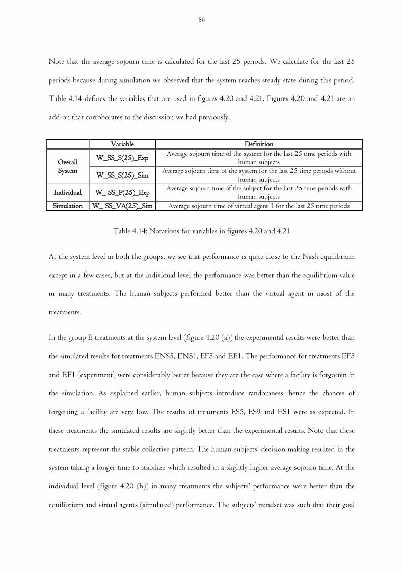
Note that the average sojourn time is calculated for the last 25 periods. We calculate for the last 25

periods because during simulation we observed that the system reaches steady state during this period.

Table 4.14 defines the variables that are used in figures 4.20 and 4.21. Figures 4.20 and 4.21 are an

add-on that corroborates to the discussion we had previously.

Variable Definition

Overall System

W_SS_S(25)_Exp Average sojourn time of the system for the last 25 time periods with

human subjects

W_SS_S(25)_Sim Average sojourn time of the system for the last 25 time periods without

human subjects

Individual W_ SS_P(25)_Exp Average sojourn time of the subject for the last 25 time periods with

human subjects

Simulation W_ SS_VA(25)_Sim Average sojourn time of virtual agent 1 for the last 25 time periods

Table 4.14: Notations for variables in figures 4.20 and 4.21

At the system level in both the groups, we see that performance is quite close to the Nash equilibrium

except in a few cases, but at the individual level the performance was better than the equilibrium value

in many treatments. The human subjects performed better than the virtual agent in most of the

treatments.

In the group E treatments at the system level (figure 4.20 (a)) the experimental results were better than

the simulated results for treatments ENS5, ENS1, EF5 and EF1. The performance for treatments EF5

and EF1 (experiment) were considerably better because they are the case where a facility is forgotten in

the simulation. As explained earlier, human subjects introduce randomness, hence the chances of

forgetting a facility are very low. The results of treatments ES5, ES9 and ES1 were as expected. In

these treatments the simulated results are slightly better than the experimental results. Note that these

treatments represent the stable collective pattern. The human subjects’ decision making resulted in the

system taking a longer time to stabilize which resulted in a slightly higher average sojourn time. At the

individual level (figure 4.20 (b)) in many treatments the subjects’ performance were better than the

equilibrium and virtual agents (simulated) performance. The subjects’ mindset was such that their goal

86

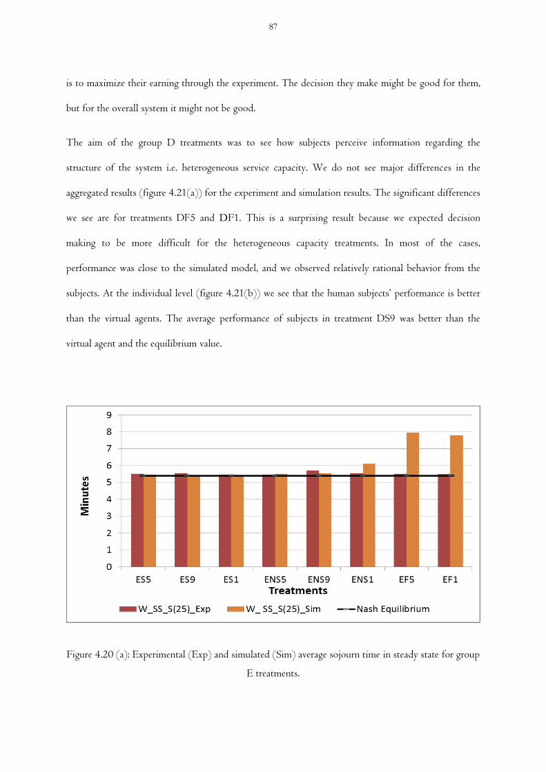
is to maximize their earning through the experiment. The decision they make might be good for them,

but for the overall system it might not be good.

The aim of the group D treatments was to see how subjects perceive information regarding the

structure of the system i.e. heterogeneous service capacity. We do not see major differences in the

aggregated results (figure 4.21(a)) for the experiment and simulation results. The significant differences

we see are for treatments DF5 and DF1. This is a surprising result because we expected decision

making to be more difficult for the heterogeneous capacity treatments. In most of the cases,

performance was close to the simulated model, and we observed relatively rational behavior from the

subjects. At the individual level (figure 4.21(b)) we see that the human subjects’ performance is better

than the virtual agents. The average performance of subjects in treatment DS9 was better than the

virtual agent and the equilibrium value.

Figure 4.20 (a): Experimental (Exp) and simulated (Sim) average sojourn time in steady state for group

E treatments.

87

Figure 4.20 (b): Experimental (Exp) and simulated (Sim) average sojourn time in steady state for group

E treatments.

Figure 4.21(a): Experimental (Exp) and simulated (Sim) average sojourn time in steady state for group

D treatments.

88

Figure 4.21(b): Experimental (Exp) and simulated (Sim) average sojourn time in steady state for group

D treatments.

We next compare the outcomes of the various treatments by using the Wilcoxon Rank-sum test. The

Wilcoxon Rank-Sum test is a non-parametric statistical test to compare two independent samples. This

test does not require that the populations have normal distributions. We use this test because i) the

sample size for each treatment is small and ii) we do not have information regarding distribution of

data. Tables 4.15 and 4.16 show the corresponding p-values for groups E and D respectively. Recall

that we refer to homogenous and heterogeneous service capacity treatments as group E and group D

treatments respectively.

We did not expect to see significant differences in group E, ‘S’ treatments, except for the treatments

which showed non-stable and forgotten facility collective behavioral patterns. Considering a 0.05

significance level, from the p-values of table 4.15, we can conclude that average sojourn time in steady

state for treatment ENS1 is on an average significantly different from treatments ES5, ENS5 and EF1.

89

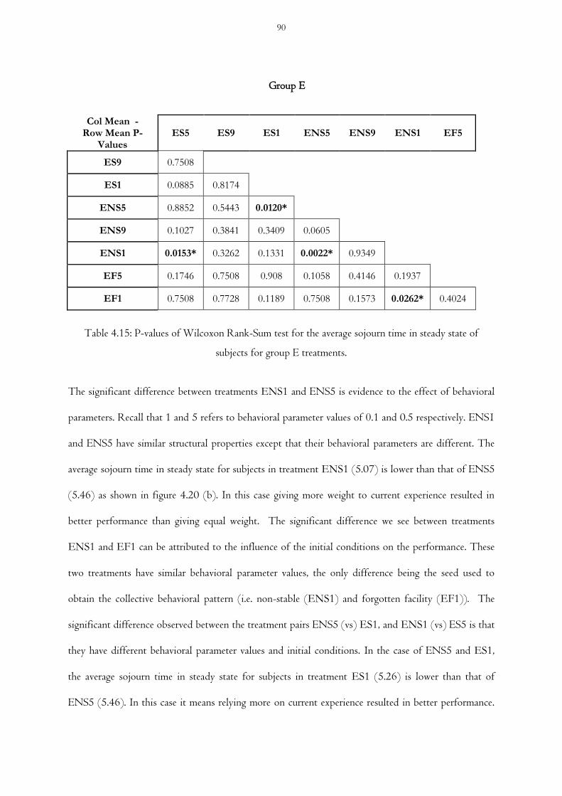
Group E

Col Mean - Row Mean P-

Values ES5 ES9 ES1 ENS5 ENS9 ENS1 EF5

ES9 0.7508

ES1 0.0885 0.8174

ENS5 0.8852 0.5443 0.0120*

ENS9 0.1027 0.3841 0.3409 0.0605

ENS1 0.0153* 0.3262 0.1331 0.0022* 0.9349

EF5 0.1746 0.7508 0.908 0.1058 0.4146 0.1937

EF1 0.7508 0.7728 0.1189 0.7508 0.1573 0.0262* 0.4024

Table 4.15: P-values of Wilcoxon Rank-Sum test for the average sojourn time in steady state of

subjects for group E treatments.

The significant difference between treatments ENS1 and ENS5 is evidence to the effect of behavioral

parameters. Recall that 1 and 5 refers to behavioral parameter values of 0.1 and 0.5 respectively. ENS1

and ENS5 have similar structural properties except that their behavioral parameters are different. The

average sojourn time in steady state for subjects in treatment ENS1 (5.07) is lower than that of ENS5

(5.46) as shown in figure 4.20 (b). In this case giving more weight to current experience resulted in

better performance than giving equal weight. The significant difference we see between treatments

ENS1 and EF1 can be attributed to the influence of the initial conditions on the performance. These

two treatments have similar behavioral parameter values, the only difference being the seed used to

obtain the collective behavioral pattern (i.e. non-stable (ENS1) and forgotten facility (EF1)). The

significant difference observed between the treatment pairs ENS5 (vs) ES1, and ENS1 (vs) ES5 is that

they have different behavioral parameter values and initial conditions. In the case of ENS5 and ES1,

the average sojourn time in steady state for subjects in treatment ES1 (5.26) is lower than that of

ENS5 (5.46). In this case it means relying more on current experience resulted in better performance.

90

4

4.5

5

5.5

6

6.5

Aver

age

sojo

urn

tim

e (m

inute

s)

(min

ute

s)

ES5 ES9 ES1 ENS5 ENS9 ENS1 EF5 EF1

The same can be said about the significant difference observed between treatments ENS1 and ES5.

ENS1’s average sojourn time in steady state for subjects (5.07) is lower than ES5’s (5.36).

Figure 4.22 uses a box and whisker plot to show the distribution of average sojourn time in steady state

of subjects for group E treatments. The box plot acts as an add-on to the Wilcoxon Rank-sum test to

show the significant difference we observed between a few treatments. There are three outliers in the

box plot. The outlier in treatment ES5 is subject 12 who earned the maximum pay-off among all the

subjects in the treatment (CHF 30). The average sojourn time of subject 12 (4.42) was well below the

average of all subjects in the treatment (5.36). The outlier in treatment EF1 is subject 5, this subject’s

performance was also well below the treatment’s average and he also earned the maximum pay-off

among all the subjects in the treatment (CHF 30). Unlike the other two outliers, the outlier (subject 9)

in treatment ENS5 did not earn the maximum pay-off.

Figure 4.22: Box plot for the average sojourn time in steady state of subjects for group E treatments.

91

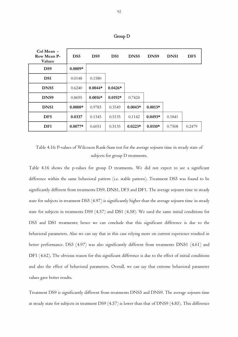
Group D

Col Mean - Row Mean P-

Values DS5 DS9 DS1 DNS5 DNS9 DNS1 DF5

DS9 0.0009*

DS1 0.0148 0.1580

DNS5 0.6240 0.0044* 0.0426*

DNS9 0.8695 0.0016* 0.0192* 0.7424

DNS1 0.0008* 0.9783 0.3549 0.0043* 0.0013*

DF5 0.0337 0.1345 0.5135 0.1142 0.0493* 0.1841

DF1 0.0077* 0.6051 0.5135 0.0223* 0.0110* 0.7508 0.2479

Table 4.16: P-values of Wilcoxon Rank-Sum test for the average sojourn time in steady state of

subjects for group D treatments.

Table 4.16 shows the p-values for group D treatments. We did not expect to see a significant

difference within the same behavioral pattern (i.e. stable pattern). Treatment DS5 was found to be

significantly different from treatments DS9, DNS1, DF5 and DF1. The average sojourn time in steady

state for subjects in treatment DS5 (4.97) is significantly higher than the average sojourn time in steady

state for subjects in treatments DS9 (4.57) and DS1 (4.58). We used the same initial conditions for

DS5 and DS1 treatments; hence we can conclude that this significant difference is due to the

behavioral parameters. Also we can say that in this case relying more on current experience resulted in

better performance. DS5 (4.97) was also significantly different from treatments DNS1 (4.61) and

DF1 (4.62). The obvious reason for this significant difference is due to the effect of initial conditions

and also the effect of behavioral parameters. Overall, we can say that extreme behavioral parameter

values gave better results.

Treatment DS9 is significantly different from treatments DNS5 and DNS9. The average sojourn time

at steady state for subjects in treatment DS9 (4.57) is lower than that of DNS9 (4.85). This difference

92

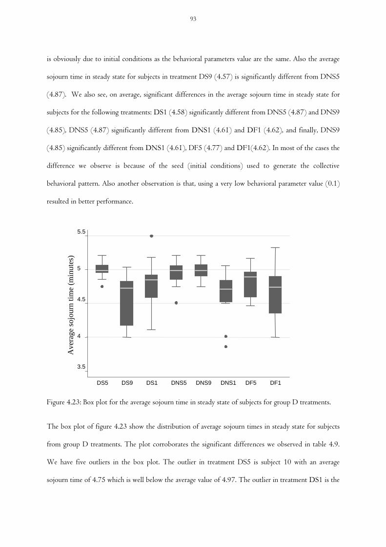
3.5

4

4.5

5

5.5

Aver

age

sojo

urn

tim

e (m

inu

tes)

(min

ute

s)

DS5 DS9 DS1 DNS5 DNS9 DNS1 DF5 DF1

is obviously due to initial conditions as the behavioral parameters value are the same. Also the average

sojourn time in steady state for subjects in treatment DS9 (4.57) is significantly different from DNS5

(4.87). We also see, on average, significant differences in the average sojourn time in steady state for

subjects for the following treatments: DS1 (4.58) significantly different from DNS5 (4.87) and DNS9

(4.85), DNS5 (4.87) significantly different from DNS1 (4.61) and DF1 (4.62), and finally, DNS9

(4.85) significantly different from DNS1 (4.61), DF5 (4.77) and DF1(4.62). In most of the cases the

difference we observe is because of the seed (initial conditions) used to generate the collective

behavioral pattern. Also another observation is that, using a very low behavioral parameter value (0.1)

resulted in better performance.

Figure 4.23: Box plot for the average sojourn time in steady state of subjects for group D treatments.

The box plot of figure 4.23 show the distribution of average sojourn times in steady state for subjects

from group D treatments. The plot corroborates the significant differences we observed in table 4.9.

We have five outliers in the box plot. The outlier in treatment DS5 is subject 10 with an average

sojourn time of 4.75 which is well below the average value of 4.97. The outlier in treatment DS1 is the

93

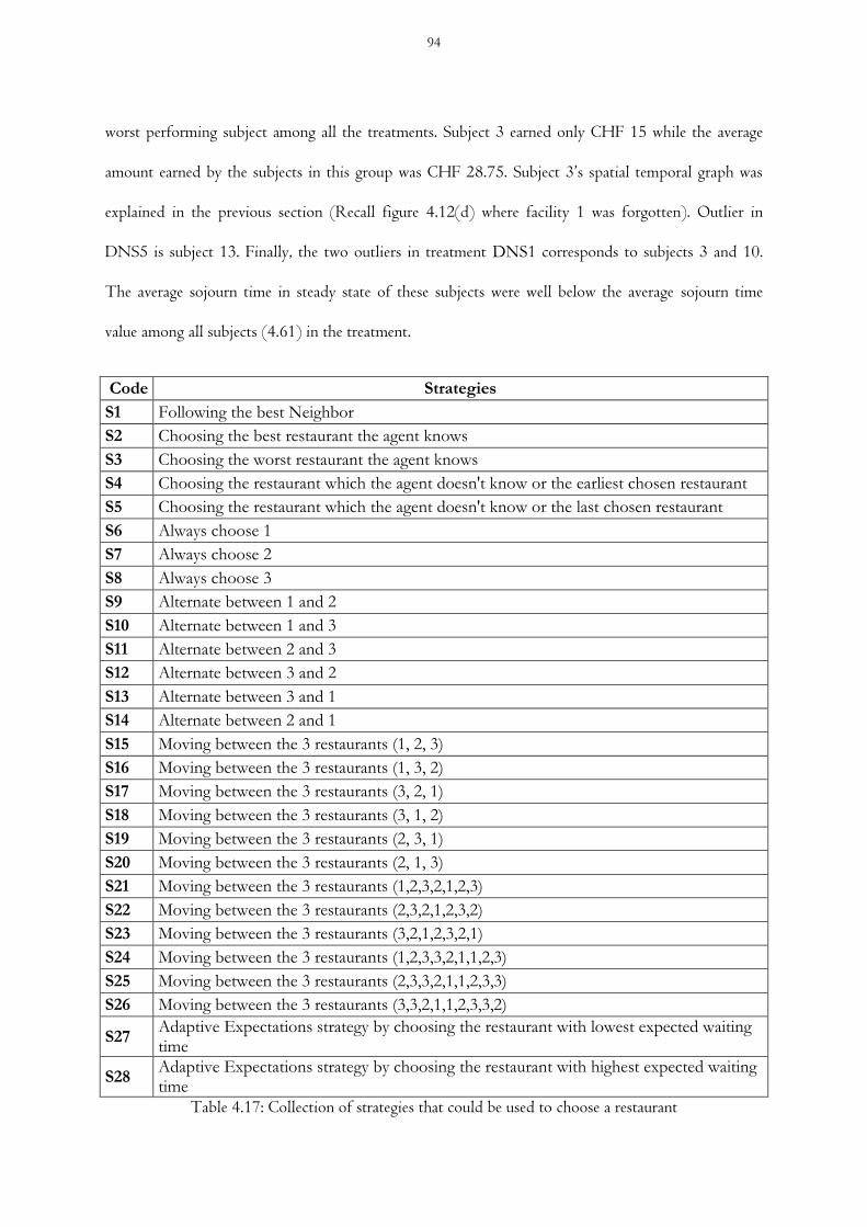
worst performing subject among all the treatments. Subject 3 earned only CHF 15 while the average

amount earned by the subjects in this group was CHF 28.75. Subject 3’s spatial temporal graph was

explained in the previous section (Recall figure 4.12(d) where facility 1 was forgotten). Outlier in

DNS5 is subject 13. Finally, the two outliers in treatment DNS1 corresponds to subjects 3 and 10.

The average sojourn time in steady state of these subjects were well below the average sojourn time

value among all subjects (4.61) in the treatment.

Code Strategies

S1 Following the best Neighbor

S2 Choosing the best restaurant the agent knows

S3 Choosing the worst restaurant the agent knows

S4 Choosing the restaurant which the agent doesn't know or the earliest chosen restaurant

S5 Choosing the restaurant which the agent doesn't know or the last chosen restaurant

S6 Always choose 1

S7 Always choose 2

S8 Always choose 3

S9 Alternate between 1 and 2

S10 Alternate between 1 and 3

S11 Alternate between 2 and 3

S12 Alternate between 3 and 2

S13 Alternate between 3 and 1

S14 Alternate between 2 and 1

S15 Moving between the 3 restaurants (1, 2, 3)

S16 Moving between the 3 restaurants (1, 3, 2)

S17 Moving between the 3 restaurants (3, 2, 1)

S18 Moving between the 3 restaurants (3, 1, 2)

S19 Moving between the 3 restaurants (2, 3, 1)

S20 Moving between the 3 restaurants (2, 1, 3)

S21 Moving between the 3 restaurants (1,2,3,2,1,2,3)

S22 Moving between the 3 restaurants (2,3,2,1,2,3,2)

S23 Moving between the 3 restaurants (3,2,1,2,3,2,1)

S24 Moving between the 3 restaurants (1,2,3,3,2,1,1,2,3)

S25 Moving between the 3 restaurants (2,3,3,2,1,1,2,3,3)

S26 Moving between the 3 restaurants (3,3,2,1,1,2,3,3,2)

S27 Adaptive Expectations strategy by choosing the restaurant with lowest expected waiting time

S28 Adaptive Expectations strategy by choosing the restaurant with highest expected waiting time

Table 4.17: Collection of strategies that could be used to choose a restaurant

94

Next we consider a collection of strategies (as shown in table 4.17) that could be adopted to choose a

restaurant/facility. These collections of strategies are not exhaustive. The following approach is taken

to extract decision making strategies adopted by subjects in the experiment. Using excel we simulated

the model using each of the strategies of table 4.17 as the decision rule for choosing the restaurant. For

example strategy S1, the restaurant chosen by the quickest neighbor is always chosen. No other

information is used. In a similar fashion the strategy S6, here, restaurant 1 is chosen all the time,

ignoring all other information. We then compare the choice of subjects with that of the simulated

model (i.e. decision rule based on strategies presented in table 4.17). The result of this approach is

portrayed in table 4.18.

From table 4.18 we can say that the strategies subjects adopted can be modeled using adaptive

expectations. In the agent based queuing model described earlier, we used adaptive expectations based

decision rules (choosing the facility with the minimum expected value). S27 accounted for 47% of

subjects in group E treatments and 56% of subjects in group D treatments. This is the same strategy

that was used in the simulation model, thus supporting the case that an adaptive expectations based

decision rule is a good way to represent human decision making. Also, S28, an adaptive expectation

based strategy, but choosing the facility with the maximum expected value is quite common among

group E treatments (33% of subjects). We also see that around 20% of subjects adopted other

strategies in group E treatments and 25% in group D treatments. Other strategies include following the

best performing neighbor, choosing the worst facility or just following facility 1 etc.

95

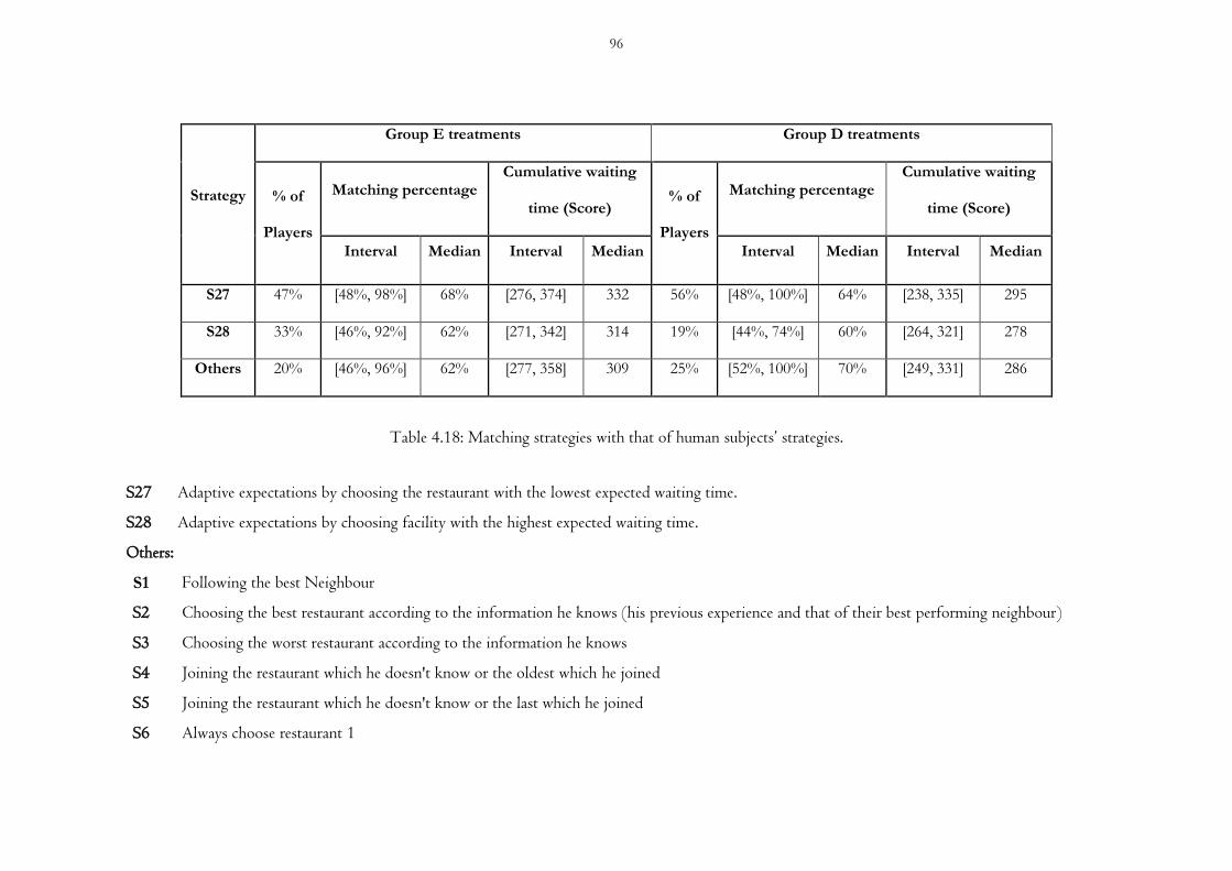
Strategy

Group E treatments Group D treatments

% of

Players

Matching percentage Cumulative waiting

time (Score) % of

Players

Matching percentage Cumulative waiting

time (Score)

Interval Median Interval Median Interval Median Interval Median

S27 47% [48%, 98%] 68% [276, 374] 332 56% [48%, 100%] 64% [238, 335] 295

S28 33% [46%, 92%] 62% [271, 342] 314 19% [44%, 74%] 60% [264, 321] 278

Others 20% [46%, 96%] 62% [277, 358] 309 25% [52%, 100%] 70% [249, 331] 286

Table 4.18: Matching strategies with that of human subjects’ strategies.

S27 Adaptive expectations by choosing the restaurant with the lowest expected waiting time.

S28 Adaptive expectations by choosing facility with the highest expected waiting time.

Others:

S1 Following the best Neighbour

S2 Choosing the best restaurant according to the information he knows (his previous experience and that of their best performing neighbour)

S3 Choosing the worst restaurant according to the information he knows

S4 Joining the restaurant which he doesn't know or the oldest which he joined

S5 Joining the restaurant which he doesn't know or the last which he joined

S6 Always choose restaurant 1

96

Through table 4.18 we show that adaptive expectations based strategies are a good way to represent

human decision making, but may not be the best approach. The results also point to the importance of

feedback i.e. information regarding the state of the system or experiences at facilities. Adaptive

expectations’ based rules are basically feedback models wherein the future state is dependent on past

states. We can link feedback to customer satisfaction, i.e. return of customers depends on their past

experiences.

For adaptive expectations based decision rules, we need to estimate the coefficient of expectations.

Table 4.19 shows these coefficients. We used the evolutionary solver in excel to estimate the

combination of behavioral coefficients (α and β) for subjects who use strategies S27 and S28 across

treatment groups. In table 4.19 (a) we show the distribution of behavioral parameter values in group E

treatments for strategy S27. 16 subjects have an α value between 0.1 and 0.9 and 19 subjects have a β

value between 0.1 and 0.9. This suggests that most of the behavioral parameter values lie within this

range. It is to be noted that there exist values very close 0.1 and 0.9 in this range. We then looked at

individual performance i.e. subjects who earned the most (CHF 30 and above) among this set of

subjects. Only 4 subjects performed extremely well. Subject 8 in treatment ES1, subject 4 in ENS1,

and subjects 7 and 9 in EF5 had performed extremely well with strategy S27. For these subjects a high

α and β resulted in good performance, except for subject 9 (treatment EF5) whose values were 0.03

and 0.4. Subjects 4 and 13 in ENS9 were the worst earning just CHF 15. For group D treatments in

table 4.19 (b) subject 10 in DNS5, subjects 2 and 7 in DNS1, subjects 7 and 11 in DF5 and subjects

4 and 6 in DF1 were the best performers. Subjects in treatment DF5 were the best in group D

treatments earning an average of CHF 29. Here also we saw α and β values to be greater than 0.7. We

can thus conclude that even though alpha and beta values for many subjects lie between 0.1 and 0.9,

this need not give the best performance.

97

Group E Group D

S27 S27

α

β

α

β

<= 0.1 0.1-0.9 >= 0.9

<=0.1 0.1-0.9 >=0.9

<= 0.1 0 10 1 11

<=0.1 1 5 0 6

0.1-0.9 2 8 6 16

0.1-0.9 3 24 7 34

>= 0.9 1 1 3 5

>=0.9 1 10 1 12

3 19 10

5 39 8

(a) (b)

S28 S28

α

β

α

β

<= 0.1 0.1-0.9 >= 0.9

<= 0.1 0.1-0.9 >= 0.9

<= 0.1 2 1 0 3

<= 0.1 1 0 0 1

0.1-0.9 7 9 0 16

0.1-0.9 3 11 1 15

>= 0.9 0 1 7 8

>= 0.9 0 5 13 18

9 11 7

4 16 14

(c) (d)

Table 4.19: Human subjects distribution across various alpha and beta values for strategies S27 and S28 among group treatments

98

Now we look at tables 4.19 (c and d) to analyze the distribution of behavioral parameters for strategy

S28. For group E treatments we see from table 4.19 (c) that 16 subjects have α value between 0.1 and

0.9 whereas β values are more or less evenly spread. We then looked at individual performance i.e.

subjects who earned the most (CHF 30 and above) among these subjects. 8 subjects performed

extremely well in this group. The beta values for all the subjects were less than 0.5 and for three

subjects less than 0.05. The alpha values had a range of 0.01 to 0.8. For the group D treatments in

table 4.19 (d) there were 15 subjects who performed extremely well i.e. earned a pay-off greater than

CHF 30. Most of the alpha and beta values were high except for a few subjects.

We can conclude that among the best performing group of subjects, high alpha (greater than 0.8) and

beta values ranging between 0.6 and 0.9 were quite common. In section 4.1 through figure 4.6 (page

41) we pointed out that relatively higher α value and medium β value results in a better performance.

This analysis makes this claim more robust.

CONCLUSION

In this paper we have shown how a simple experimental set up can be used to validate a behavioral

queuing model. We first introduce the behavioral queuing framework. Simulation indicates that at the

aggregate level the system might look stable but, at the individual level, it might not be the case. The

individual behavior is a useful level at which we can understand how agents learn about the system,

update their information and thus adapt.

Then, human subjects take the role of a virtual agent in an experiment, and choose a service facility

every time period based on past experience and local information. We see from the results that human

subjects who take the role of virtual agents have a significant influence on the collective behavior. We

interpret that human subjects introduce randomness, hence not forgetting a facility in most of the

situations. Only in rare cases is a facility forgotten. Looking at the aggregated results we see that

99

generally system level performance is quite bad compared to the equilibrium value, but many a times at

the individual level, subjects performed better than the Nash equilibrium. This answers the question

that we raised regarding the effect of a single human subject on the performance of the system and how

subjects adapt based on the behavior of the system. We also saw that the collective patterns we observe

in the experiment are comparable to that of the simulated results.

Through the Wilcoxon test we explain why the treatments have significant differences. We show the

influence of initial conditions and behavioral parameters on the average sojourn time of the subjects

and also on the subjects’ decision making. We then illustrate that an adaptive expectations based

strategies are a good way to represent human decision making, but may not be the best as far as

performance is concerned. This validates the decision rule (based on adaptive expectations) that we

proposed in the simulation model. Finally, we show the distribution of behavioral parameters alpha and

beta for the adaptive expectations based strategies. For the adaptive expectation strategy where the

restaurant is chosen with the lowest expected waiting time, alpha and beta values greater than 0.7

resulted in better performance. High alpha value (greater than 0.8) and beta values between 0.6 and 0.9

were common in adaptive expectation strategy where the restaurant with the highest expected waiting

time is chosen. This result corroborates with the findings of the first paper.

As a part of future work, further exploration of experimental data might give a better idea regarding

how subjects perceive information. We had provided them with a questionnaire concerning what

information they used to make decisions. We can use the answers to understand how the subjects

process information and what information they use for decision making.

100

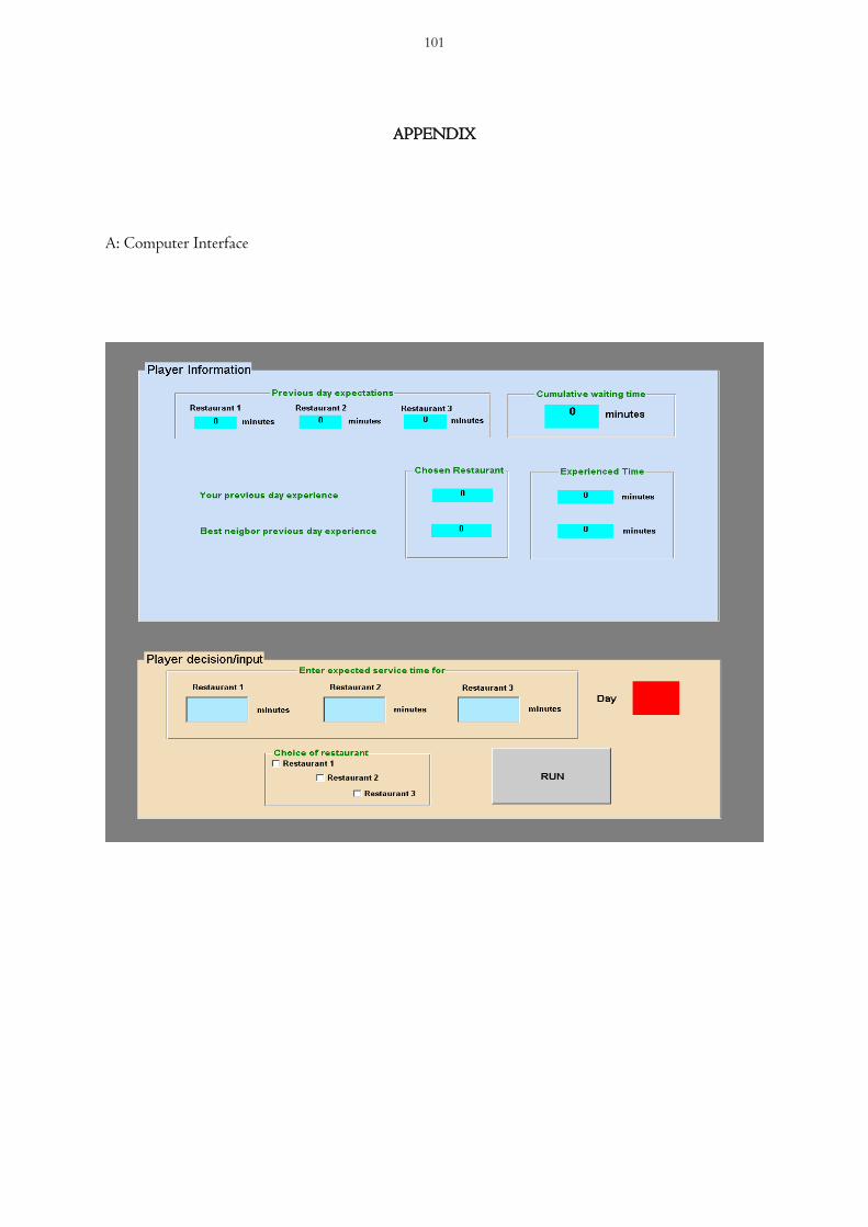
APPENDIX

A: Computer Interface

101

B: Subject Instructions (Base case treatment ES5)

“A tale of three restaurants”

Instructions for the participants

NOTE: PLEASE DO NOT TOUCH THE COMPUTER BEFORE BEING ASKED TO DO SO

Welcome to the experiment on decision making in a service industry. The instructions for this

experiment are simple. If you follow them carefully and make good decisions, you may earn up to CHF

35 (the money will be credited to your bank account). You are free to halt the experiment at any time

without notice. However, if you do not pursue the experiment until the end, you will not receive any

payment. This experiment is funded by the Swiss National Science Foundation (Grant

100014_126584). If you have any questions before or during the experiment, please feel free to raise

your hand and a monitor will come to assist you.

We assure you that the data we collect during the course of this experiment will be held in strict

confidence. Anonymity is guaranteed; information will not be reported in any manner or form that

would allow associating names with individual players.

Description of Experiment

This experiment has been designed to study how individual members of a population choose a service

facility based upon their expectations and past experiences. Below is a short explanation of the system

you will interact with during the experiment. It is a relatively simple system where you have to make

one decision each time period (the choice of a service facility) and provide estimates of the time you

would expect to spend at each of the service facilities.

102

The situation

You are a student at the university and everyday during lunch time, i.e. at 12:00, you have three

restaurants (the service providers) to choose from for lunch. The three restaurants have similar pricing

and offer food of comparable quality. They are located in three different parts of the campus, at equal

distance from you. Consequently, you must make your choice before observing the crowd at the

different restaurants.

In the experiment, you will be playing with virtual customers who have the same task, i.e., to decide

which restaurant to join every day. Thus you will be queuing with some of them in your chosen

restaurant. Once you decide which restaurant to use, you cannot change your decision, you must wait

for service.

The Waiting time is the time between the moment you arrive and the moment you receive your meal.

This time depends on how many people (virtual customers and you) have chosen that restaurant and

the service capacity of the restaurant.

The Service Capacity is the number of customers a restaurant can, on average, service per minute. The

three facilities have the same service capacity (5 customers/ minute), which remains constant

throughout the experiment.

Your Expected waiting time is time that you expect to spend at the different restaurants. At the start of

the experiment initial estimates for each restaurant will be provided.

Information available: each period you will be informed of the waiting time at your chosen facility. You

also have two virtual neighbors who will inform you of the restaurant they selected and how long they

waited.

103

Your Task

As a customer, you must decide each day where to go for lunch. Your goal for this experiment will be

to minimize the total waiting time over the 60 simulated days (i.e. the sum of your daily waiting times

over these 60 days) by choosing each day the restaurant you believe will have the shortest waiting time

that day. You will need approximately 1 hour to complete the experiment.

To help you make this decision you will receive the following information each day:

1) The time you waited at the restaurant you selected the previous day

2) Your previous waiting time expectations for the three restaurants , and

3) The information from your virtual neighbors about their previous choice and experienced

waiting time.

Each day you will enter into the graphical user interface of the experiment the following information:

1) Your choice of restaurant and

2) Your expectation of waiting time at each of the three restaurants

Interface

All the interaction will take place through the interface on your computer screen. The information is

the same as what we have provided in these instructions. Please ask the facilitator to have a trial run to

test out the software.

104

Payment

Please note that if you want to participate in this experiment you must sign the consent form on your

desk. This form must be signed before the start of the experiment.

The payment for this experiment consists of a guaranteed participation fee of CHF 15, plus a bonus

which will depend on your performance. Your performance is measured by your total waiting time over

the 60-day experiment. The lower your total waiting time, the larger the bonus you will receive. This

bonus will vary between CHF 0 and CHF 20.

If you do not pursue the experiment until the end, you will not receive any payment.

At the end of the experiment, you will be asked to complete and sign a form with your name, student

ID number, email address, account information and amount earned, and indicating whether or not you

are employed by the university.

We will be happy to answer any questions you may have concerning this experiment.

If you have no further questions, please ask the experiment facilitator to begin. Good luck and enjoy

the experiment!

105

CHAPTER 5: CONCLUSION

Queuing is a very common phenomena that we witness and encounter on a day to day basis. Queuing

theory and its problems span a broad range of applications and have been studied extensively in various

disciplines. Traditional queuing research has relied more on analytical techniques and focused on

designing an efficient system. These analytical models assumed static conditions, exogenous arrival and

service rates, and were analyzed in steady-state. On the contrary, most queuing systems are dynamic,

and the customers using the system make decisions based on their perception of the state of the system.

The decision processes of customers who use these queuing systems have also been largely neglected.

Quite recently researchers have attempted to move away from this classical approach of queuing. This

dissertation is in line with such a trend and looks into the micro-dynamics of queuing to understand

the formation of queues. The main contribution of this dissertation is towards the field of behavioral

operations and emphasizes the need to incorporate behavioral and cognitive factors into the models

(Gino and Pisano, 2008).

The bulk of the thesis consists of three research papers. The first paper sets the tone for the thesis and

its contributions. The key contribution of this paper is the use of agent based modeling as a

methodology for the study of queue formation. The idea is to investigate the micro features i.e.

individual decision making and the macro consequences for the system. The primary aim of this paper

is to emphasize the need to look at the spatial temporal dimension in order to understand expectation

formation, and in turn, its influence on decision making. Also looking at the individual level helps to

see how information diffuses and how this information is used in decision making. This is relevant for

service facilities we encounter on a day to day basis like traffic, supermarkets etc. By introducing an

agent based queuing model the thesis has opened up avenues for future research in the area of

behavioral operations (Gino and Pisano, 2008).

106

The second paper takes the agent based framework one step further by modeling a population of CA’s

who evolve based on the consequences of their queuing. The key contribution of this paper is the use

of genetic algorithms to model CA’s (each of which consists of agents) who optimize their behavior by

learning from the system. The agents learn and choose the service facility based on past experience and

the local information available to them. This model works at the population level and optimizes the

performance of the system. The results of the paper show how genetic algorithms improve the

performance of the CA model and bring the overall system performance close to the Nash equilibrium.

The contribution of this paper is that it further develops the intelligence of decision makers in the

agent based model. It enables the population of CA’s to change behavioral parameters, thus allowing

them to adapt behavior based on their experiences.

The third paper shows how an experiment can be designed to investigate and validate the behavioral

queuing model presented in the first paper. The main contribution of this paper is the use of

experimental methods to validate the agent based queuing model. This approach follows the approach

of Sterman (1987, 1989) and Rapoport (2004), who use experimental methods to understand decision

making. The paper shows how to design an experimental setup by using the agent based behavioral

queuing framework. A human subject replaces a virtual agent in the agent based model and decides the

facility to use based on the information available to them. The aim of this approach is to validate the

findings of the agent based model and also to see what strategies subjects adopt to choose the service

facility. The experiment shows that human subjects have a significant influence on the overall system

behavior. The paper also shows that adaptive expectations based decision rules are a good way to

represent human decision making. This paper thus contributes towards the psychology of queuing, and

the use of experimental methods to build confidence in decision making simulation models.

The key contribution of this thesis is towards the area of behavioral operations. Through three

scholarly papers the thesis shows how a behavioral framework can be modeled, simulated and validated.

107

Also the thesis shows that by adopting methodologies like agent based simulation and experimental

methods, one can limit assumptions that simplify system complexity. This results in models that are

closer to real life queuing problems. The thesis not only contributes to the areas of operations research

and management science, but its findings can be applied to other disciplines like manufacturing,

information systems, industrial engineering to name a few. The table 4.17 shows the positioning of the

three papers presented in the thesis and the conference papers to which I contributed pointing, to the

contribution made to literature.

LIMITATION AND FUTURE WORK

The dissertation is not without limitations and the following paragraphs addresses those limitations

and the avenues for future work.

The agent model presented in the dissertation is a neighborhood based system which is relevant to

understand social processes that we encounter. The structure of the model is such that each agent

interacts with a fixed number of neighbors. This is a limitation, because, in reality this is not fixed.

This could be easily rectified in the model by having heterogeneous neighborhood sizes, but the idea

was to show how a simple agent based framework can help us understand the micro-dynamics of

queuing.

The agents in the model are homogenous except for their location in the one-dimensional lattice and

initial conditions. The model has synchronous updating; agents follow similar expectation formation

and have identical computational capabilities. These are reasonable at the cellular level but not in

reality. The aim of the model is to show how a simple self-organizing agent based queuing system can

be designed. The model helps us to understand the micro-dynamics of queuing and the effects of

individual decision making on the performance of the system. This limitation can be resolved by having

heterogeneous agents with different decision making strategies and computational capabilities.

108

Stochastic Deterministic

Analytical Simulation Experimental Analytical Simulation Experimental

Arrival rate exogenous Edelson and

Hildebrand (1975) Agnew (1976)

Arrival rate endogenous

& service rate

exogenous

State dependent

Naor (1969) Yechiali (1971)

Boots and Tijms (1999)

Whitt (1999)

van Ackere (1995)

(Sankaranarayanan et al., 2011c)

(Sankaranarayanan et al., 2011b)

(Sankaranarayanan et al., 2011a)

(Sankaranarayanan et al., 2010)

(Sankaranarayanan et al., 2009)

(Delgado et al., 2011b)

(Delgado et al., 2011a)

Rapoport (2004, 2010)

Stein et al. (2007) (Sankaranarayanan

et al., 2011d)

Steady state Dewan and

Mendelson (1990) Stidham (1992)

Zohar et al. (2002) Edelson (1971)

Dynamic Rump and Stidham

(1998) Seale et al. (2005)

Arrival and service rate endogenous

Steady state Ha (1998, 2001) Agnew (1976)

Dynamic

Haxholdt et al. (2003)

van Ackere and Larsen (2004)

van Ackere et al. (2006)

van Ackere et al. (2010)

Table 4.20: Contribution to literature

109

MATLAB is an extremely useful scientific tool and extensively used by researchers. MATLAB works at

the matrix level and stores matrices in contiguous blocks of virtual memory. Hence, the largest matrix

that can be created and stored is limited by the computers contiguous free virtual space available. The

dissertation presented a one-dimensional agent based framework and MATLAB worked fine. If a two-

dimensional model is to be developed and the K-neighborhood increased, then we need to look at agent

based toolkits like Repast, Mason etc. for modeling.

As a part of future work, an interesting extension to the CA model would be to have complex rules or

mixed strategy rules for agents. In this way agents decide what rule to use based on the state of the

system. Concerning the GA, at the methodological level an interesting approach would be to investigate

other heuristic search techniques and compare them with the GA. Another interesting extension to the

framework is to add another group of agents, the managers of the facility. They will compete for

customers by optimizing their facility based on customers’ reactions.

The experiment we designed was based on the agent based model. We replaced a single virtual agent

with a human subject and found interesting collective behavior. We thus had 119 virtual agents and a

human subject interacting. An extension for the experimental study is to have only human subjects; this

would be a network game wherein subjects will have specific human neighbors’ (friends, colleagues etc.)

and thus not interacting with virtual agents who follow specific rules. Finally, more results could be

squeezed out of the data collected through the experiment. For example, we had asked the subjects to

answer a questionnaire after completing the experiment. The first question concerns the strategy

adopted for choosing a restaurant, and the second one related to the information they used to make

their decisions. We can use this to find out how subjects perceive information.

110

BIBLIOGRAPHY

A. K.Y. Law, Y.V. Hui and X. Zhao (2004). "Modeling repurchase frequency and customer

satisfaction for fast food outlets." International Journal of Quality & Reliability Management

21(5): 545-563.

Agnew, C. E. (1976). "Dynamic modeling and control of congestion-prone systems." Operations

Research 24(3): 400-419.

Aksin, Z. N., M. Armony and V. Mehrotra (2007). "The modern call center: A multi-disciplinary

perspective on operations management research." Production and Operations Management

16(6): 665-688.

Axelrod, R. M. (1997). The complexity of cooperation : Agent-based models of competition and

collaboration. Princeton, NJ [u.a.], Univ. Press.

Bandini, S., R. Casati, E. Illy, C. Simone, F. S. Liverani, F. Tisato and C. Assoc Sci Int (1997). A

reaction-diffusion computational model to simulate coffee percolation.

Bendoly, E., R. Croson, P. Goncalves and K. Schultz (2010). "Bodies of knowledge for research in

behavioral operations." Production and Operations Management 19(4): 434-452.

Benjamin, S. C., N. F. Johnson and P. M. Hui (1996). "Cellular automata models of traffic flow along

a highway containing a junction." Journal of Physics a-Mathematical and General 29(12):

3119-3127.

Bielen, F. and N. Demoulin (2007). "Waiting time influence on the satisfaction-loyalty relationship in

services." Managing Service Quality 17(2): 174-193.

Bonabeau, E. (2002). "Agent-based modeling: Methods and techniques for simulating human

systems." Proceedings of the National Academy of Sciences of the United States of America

99: 7280-7287.

Boots, N. K. and H. Tijms (1999). "A multiserver queueing system with impatient customers."

Management Science 45(3): 444-448.

Bruderer, E. and J. V. Singh (1996). "Organizational evolution, learning, and selection: A genetic-

algorithm-based model." Academy of Management Journal 39(5): 1322-1349.

Caruso, G., D. Peeters, J. Cavailhes and M. Rounsevell (2007). "Spatial configurations in a periurban

city. A cellular automata-based microeconomic model." Regional Science and Urban

Economics 37(5): 542-567.

Casti, J. L. (1997). Would-be worlds : How simulation is changing the frontiers of science. New York

[u.a.], Wiley.

111

Darwin, C. and E. O. Wilson (2006). From so simple a beginning : The four great books of charles

darwin. New York [u.a.], Norton.

Delgado, C. A., A. van Ackere, E. R. Larsen and K. Sankaranarayanan (2011a). Modelling decisions

under uncertainty in a behavioural queuing system. 25th European Conference on Modelling

and Simulation, Krakow, Poland, June 7 to 10, 2011.

Delgado, C. A., A. van Ackere, K. Sankaranarayanan and E. R. Larsen (2011b). Collective behavioural

patterns in a multichannel service facilities system: A cellular automata approach. 12th

INFORMS Computing Society Conference, Monterey, CA, INFORMS.

Deutsch, A. and S. Dormann (2005). Cellular automaton modeling of biological pattern formation :

Characterization, applications, and analysis. Boston, Mass. [u.a.], Birkhäuser.

Dewan, S. and H. Mendelson (1990). "User delay costs and internal pricing for a service facility."

Management Science 36(12): 1502-1517.

Edelson, N. M. (1971). "Congestion tolls under monopoly." American Economic Review 61(5): 873-

882.

Edelson, N. M. and D. K. Hildebrand (1975). "Congestion tolls for poisson queuing processes."

Econometrica 43(1): 81-92.

Epstein, J. M., R. L. Axtell and Brookings Institution (1996). Growing artificial societies : Social

science from the bottom up ; a product of the 2050 project, a collaborative effort of the

brookings institution, the santa fe institute, and the world resources institute. Washington, DC

[u.a.], Brookings Inst. Press [u.a.].

Erlang, A. K. (1909). "The theory of probabilities and television conversations." Matematisk

Tidsskrift B: 13.

Fogel, L. J. (1999). Intelligence through simulated evolution : Forty years of evolutionary

programming. New York [u.a.], Wiley.

Friedman, D. and S. Sunder (1994). Experimental methods : A primer for economists. Cambridge

[u.a.], Cambridge Univ. Press.

Gans, N. and Y. P. Zhou (2003). "A call-routing problem with service-level constraints." Operations

Research 51(2): 255-271.

Gardner, E. S. (2006). "Exponential smoothing: The state of the art - part ii." International Journal of

Forecasting 22(4): 637-666.

Gen, M. and R. Cheng (1997). Genetic algorithms and engineering design. New York [u.a.], Wiley.

Gilbert, G. N. and K. G. Troitzsch (2005). Simulation for the social scientist. Maidenhead [u.a.],

Open Univ. Press.

112

Gino, F. and G. Pisano (2008). "Toward a theory of behavioral operations." M&Som-Manufacturing

& Service Operations Management 10(4): 676-691.

Goldberg, D. E. (2009). Genetic algorithms in search, optimization, and machine learning. Boston

[u.a.], Addison-Wesley.

Gross, D. and C. M. Harris (1998). Fundamentals of queueing theory. New York, NY [u.a.], Wiley.

Grossklags, J. (2007). Experimental economics and experimental computer science: A survey.

Experimental computer science on Experimental computer science. San Diego, USENIX

Association.

Guala, F. (2008). Experimental economics, history of. The new palgrave dictionary of economics.

Basingstoke, Palgrave Macmillan.

Gutowitz, H. (1991). Cellular automata : Theory and experiment. Cambridge, Mass. [u.a.], MIT Press.

Ha, A. Y. (1998). "Incentive-compatible pricing for a service facility with joint production and

congestion externalities." Management Science 44(12): 1623-1636.

Ha, A. Y. (2001). "Optimal pricing that coordinates queues with customer-chosen service

requirements." Management Science 47(7): 915-930.

Hassin, R. and M. Haviv (2003). To queue or not to queue : Equilibrium behavior in queueing

systems. Boston [u.a.], Kluwer Academic Publ.

Haupt, R. L. and S. E. Haupt (2004a). Practical genetic algorithms. Hoboken, NJ, Wiley-Interscience.

Haupt, R. L. and S. E. Haupt (2004b). Practical genetic algorithms. Hoboken, NJ, Wiley.

Haxholdt, C., E. R. Larsen and A. van Ackere (2003). "Mode locking and chaos in a deterministic

queueing model with feedback." Management Science 49(6): 816-830.

Heims, S., J. v. Neumann and N. Wiener (1984). John von neumann and norbert wiener : From

mathematics to the technologies of life and death. Cambridge, Mass., MIT Press.

Holland, J. H. (1992). "Genetic algorithms." Scientific American 267(1): 66-72.

Holland, J. H. (2001). Adaptation in natural and artificial systems : An introductory analysis with

applications to biology, control, and artificial intelligence. Cambridge [u.a.], MIT Press.

Holland, J. H. and J. H. Miller (1991). "Artificial adaptive agents in economic-theory." American

Economic Review 81(2): 365-370.

Hurd, P. L. and S. Hamblin (2007). "Genetic algorithms and non-ess solutions to game theory

models." Animal Behaviour 74: 1005-1018.

Ilachinski, A. (2002). Cellular automata : A discrete universe. Singapore [u.a.], World Scientific.

Kendall, D. G. (1951). "Some problems in the theory of queues." Journal of the Royal Statistical

Society Series B-Statistical Methodology 13(2): 151-185.

113

Kendall, D. G. (1953). "Stochastic processes occurring in the theory of queues and their analysis by the

method of the imbedded markov chain." Annals of Mathematical Statistics 24(3): 338-354.

Koole, G. and A. Mandelbaum (2002). "Queueing models of call centers: An introduction." Annals of

Operations Research 113(1-4): 41-59.

Little, J. D. C. (1961). "A proof for the queuing formula - l=lambda-w." Operations Research 9(3):

383-387.

Loch, C. H. and Y. Z. Wu (2008). "Social preferences and supply chain performance: An experimental

study." Management Science 54(11): 1835-1849.

Lomi, A. and E. R. Larsen (1996). "Interacting locally and evolving globally: A computational

approach to the dynamics of organizational populations." Academy of Management Journal

39(5): 1287-1321.

Lomi, A., E. R. Larsen and A. van Ackere (2003). "Organization, evolution and performance in

neighborhood-based systems." Geography and Strategy 20: 239-265.

Macal, C. M. and M. J. North (2006). "Tutorial on agent-based modeling and simulation part 2: How

to model with agents." Proceedings of the 2006 Winter Simulation Conference, Vols 1-5: 73-

83.

Mellouli, S., B. Moulin and G. Mineau (2003). "Laying down the foundations of an agent modelling

methodology for fault-tolerant multi-agent systems." Engineering Societies in the Agents

World Iv 3071: 275-293.

Mendelson, H. and U. Yechiali (1981). "Controlling the gi-m-l queue by conditional acceptance of

customers." European Journal of Operational Research 7(1): 77-85.

Miller, J. H. and S. E. Page (2007). Complex adaptive systems : An introduction to computational

models of social life. Princeton, NJ [u.a.], Princeton Univ. Press.

Mitchell, M. (2001). An introduction to genetic algorithms. Cambridge, Mass. [u.a.],.

Moon, C., J. Kim, G. Choi and Y. Seo (2002). "An efficient genetic algorithm for the traveling

salesman problem with precedence constraints." European Journal of Operational Research

140(3): 606-617.

Naor, P. (1969). "Regulation of queue size by levying tolls." Econometrica 37(1): 15-24.

Nerlove, M. (1958). "Adaptive expectations and cobweb phenomena." Quarterly Journal of

Economics 73(2): 227-248.

North, M. J. and C. M. Macal (2007). Managing business complexity : Discovering strategic solutions

with agent-based modeling and simulation. Oxford [u.a.], Oxford Univ. Press.

114

Rapoport, A., W. E. Stein, V. Mak, R. Zwick and D. A. Seale (2010). "Endogenous arrivals in batch

queues with constant or variable capacity." Transportation Research Part B-Methodological

44(10): 1166-1185.

Rapoport, A., W. E. Stein, J. E. Parco and D. A. Seale (2004). "Equilibrium play in single-server

queues with endogenously determined arrival times." Journal of Economic Behavior &

Organization 55(1): 67-91.

Rechenberg, I. (1965). "Cybernetic solution path of an experimental problem. ." Library Translation

1122, Royal Aircraft Establishment, Farnborough, UK.

Rechenberg, I. (1994). Evolutionsstrategie '94. Stuttgart, Frommann-Holzboog.

Reeves, C. R. (1997). "Genetic algorithms for the operations research." INFORMS Journal on

computing 9(3): 231-250.

Rump, C. M. and S. Stidham (1998). "Stability and chaos in input pricing for a service facility with

adaptive customer response to congestion." Management Science 44(2): 246-261.

Samuelson, D. A. (2000). "Designing organizations." ORMS Today 27(6).

Samuelson, D. A. (2005). "Agents of change: How agent-based modeling may transform social

science." ORMS Today 32(1).

Samuelson, D. A. and C. M. Macal (2006). "Agent-based simulation comes of age." ORMS Today

33(4): 34-38.

Sankaranarayanan, K., C. A. Delgado, A. van Ackere and E. R. Larsen (2011a). Behavioural queuing:

An agent based modelling approach. Proceedings of the 2011 3rd International conference on

Computer Modelling and Simulation (ICCMS 2011). Mumbai, India.

Sankaranarayanan, K., C. A. Delgado, A. van Ackere and E. R. Larsen (2011b). The micro-dynamics of

queuing: Understanding the formation of queues. Institute of Management, University of

Lugano, Swirtzerland. Working paper.

Sankaranarayanan, K., C. A. Delgado, A. van Ackere and E. R. Larsen (2011c). Modelling decision

making in an agent based queueing system using cellular automat and genetic algorithms.

Institute of Management, University of Lugano, Switzerland. Working paper.

Sankaranarayanan, K., C. A. Delgado, A. van Ackere and E. R. Larsen (2011d). A tale of three

restaurants: An experimental approach to understanding decision making in queueing systems.

Institute of Management, University of Lugano, Switzerland. Working paper.

Sankaranarayanan, K., E. R. Larsen and A. van Ackere (2009). Intelligent agents behavior in the

queueing process: Integrating cellular automata & genetic algorithms. 2009 Ieee International

Conference on Industrial Engineering and Engineering Management, Vols 1-4.

115

Sankaranarayanan, K., E. R. Larsen, A. van Ackere and C. A. Delgado (2010). Genetic algorithm based

optimization of an agent based queuing system. Industrial Engineering and Engineering

Management (IEEM), 2010 IEEE International Conference on.

Schelling, T. C. (2005). The strategy of conflict. Cambridge, Mass. [u.a.], Harvard Univ. Press.

Seale, D. A. (2005). "Joining a queue or staying out: Effects of information structure and service time

on arrival and staying out decisions." Experimental Economics 8(2): 117-144.

Siegel, S. and L. E. Fouraker (1960). Bargaining and group decision making: Experiments in bilateral

monopoly, McGraw-Hill.

Simon, H. A. (1979). "Rational decision-making in business organizations." American Economic

Review 69(4): 493-513.

Smith, V. L. (1982). "Microeconomic systems as an experimental science." American Economic

Review 72(5): 923-955.

Smith, V. L. (1989). "Theory, experiment and economics." Journal of Economic Perspectives 3(1):

151-169.

Sonnemans, J., C. Hommes, J. Tuinstra and H. van de Velden (2004). "The instability of a

heterogeneous cobweb economy: A strategy experiment on expectation formation." Journal of

Economic Behavior & Organization 54(4): 453-481.

Stein, W. E., A. Rapoport, D. A. Seale, H. T. Zhang and R. Zwick (2007). "Batch queues with choice

of arrivals: Equilibrium analysis and experimental study." Games and Economic Behavior

59(2): 345-363.

Sterman, J. D. (1987). "Testing behavioral simulation-models by direct experiment." Management

Science 33(12): 1572-1592.

Sterman, J. D. (1989). "Modeling managerial behavior - misperceptions of feedback in a dynamic

decision-making experiment." Management Science 35(3): 321-339.

Stidham, S. (1985). "Optimal-control of admission to a queuing system." Ieee Transactions on

Automatic Control 30(8): 705-713.

Stidham, S. (1992). "Pricing and capacity decisions for a service facility - stability and multiple local

optima." Management Science 38(8): 1121-1139.

Stidham, S. and R. R. Weber (1989). "Monotonic and insensitive optimal policies for control of

queues with undiscounted costs." Operations Research 37(4): 611-625.

van Ackere, A. (1995). "Capacity management: Pricing strategy, performance and the role of

information." International Journal of Production Economics 40(1): 89-100.

116

van Ackere, A., C. Haxholdt and E. R. Larsen (2006). "Long-term and short-term customer reaction:

A two-stage queueing approach." System Dynamics Review 22(4): 349-369.

van Ackere, A., C. Haxholdt and E. R. Larsen (2011). "Dynamic capacity adjustments with reactive

customers." Working paper 0814.

van Ackere, A. and E. R. Larsen (2004). "Self-organising behaviour in the presence of negative

externalities: A conceptual model of commuter choice." European Journal of Operational

Research 157(2): 501-513.

van Ackere, A. and E. R. Larsen (2007). "Queueing: A behavioural approach." Swiss National Science

Foundation (SNF) research proposal form No.100014_1265.

van Ackere, A. and E. R. Larsen (2009). "Queueing: A behavioural approach." Swiss National Science

Foundation (SNSF) research proposal form No.100014_1265.

Von Neumann, J. and O. Morgenstern (2007). Theory of games and economic behavior. Princeton,

N.J. [u.a.], Princeton Univ. Press.

Wahle, J., L. Neubert, J. Esser and M. Schreckenberg (2001). "A cellular automaton traffic flow model

for online simulation of traffic." Parallel Computing 27(5): 719-735.

Whitt, W. (1999). "Improving service by informing customers about anticipated delays." Management

Science 45(2): 192-207.

Wolfram, S. (1983). "Statistical-mechanics of cellular automata." Reviews of Modern Physics 55(3):

601-644.

Wolfram, S. (1984). "Cellular automata as models of complexity." Nature 311(5985): 419-424.

Wolfram, S. (2002). Cellular automata and complexity : Collected papers. Boulder, Co, Westview-

Press.

Yechiali, U. (1971). "Optimal balking rules and toll charges in gi/m/1 queuing process." Operations

Research 19(2): 347-370.

Yechiali, U. and P. Naor (1971). "Queuing problems with heterogeneous arrivals and service."

Operations Research 19(3): 722-&.

Zohar, E., A. Mandelbaum and N. Shimkin (2002). "Adaptive behavior of impatient customers in tele-

queues: Theory and empirical support." Management Science 48(4): 566-583.

117