STUDY OF TWO-PHASE FLOWS IN FUSION MAGNETS

STUDY OF TWO-PHASE FLOWS IN FUSION MAGNETS

By

GAURAV KUMAR SINGH

ENGG06201404001

INSTITUTE FOR PLASMA RESEARCH, GANDHINAGAR

A thesis submitted to the

Board of Studies in Engineering Sciences

In partial fulfillment of requirements

For, the Degree of

DOCTOR OF PHILOSOPHY

of

HOMI BHABHA NATIONAL INSTITUTE

May, 2019

List of Publications arising from the thesis

Journal

1. “Prediction of helium vapor quality in steady state Two-phase operation of

SST-1 Superconducting Toroidal field magnets”, G. K. Singh, Rohit Panchal,

Vipul Tanna, Subrata Pradhan, IEEE Transactions on Applied Superconductivity,

March 2018, Vol. 28, Issue: 2.

2. “Development of a Precise electronic system for cryogenic two-phase flow

void fraction measurement”, G. K. Singh, G. Purwar, Rakesh Patel, Hiren

Nimavat, Vipul Tanna, Journal of Electrical and Electronics Engineering, Oct.

2018, Vol. 11, nr. 2, 27-30.

3. “Experimental studies of two-phase flow characteristics and void fraction

prediction in horizontal two-phase nitrogen flow”, G.K.Singh, Subrata Pradhan,

Vipul Tanna, Cryogenics, June 2019, Vol. 100, Pages 77-84.

Conferences

1. “Experimental Investigation of two-phase nitrogen Cryo transfer line”, G. K.

Singh, Hiren Nimavat, Rohit Panchal, Atul Garg, GLN Srikanth, Ketan Patel,

Pankil Shah, Vipul Tanna, Subrata Pradhan , 26th

International Cryogenics

Engineering Conference (ICEC26)–International Cryogenic Material Conference

(ICMC), New Delhi, India ,March 7-11, 2016.

2. “Lab scale design, fabrication of Cryo line to study and analysis two-phase

flow characteristics using Liquid Nitrogen”, G. K. Singh, Hiren Nimavat, Rohit

Panchal, Atul Garg, GLN Srikanth, Ketan Patel, Pankil Shah, Vipul Tanna,

Dedicated to my family

ACKNOWLEDGEMENTS

Foremost, I would like to express my sincere gratitude to my advisor Dr. Vipul Tanna for the

continuous support of my Ph.D. study and research, for his patience, motivation, enthusiasm, and

immense knowledge. From the day I have joined him, I have received his unfailing support and

unparalleled wisdom regarding not only my research area but also his general approach to

solving problems. I have greatly benefited from my interactions with him, despite his busy

schedule, he has always been there to help me at critical junctures of my research work. I have

also learned how to handle pressure, organize my approach to studying literature and

formulating useful research problems from him. In addition to the formal aspects of the thesis

work, I have also enjoyed the numerous freewheeling discussions we have had, which have

motivated my research work and also inspired towards success in my life. I will be eternally

grateful for the time I have spent with him and will always try to live up to the high standards he

has set as leading scientist.

During my PhD, Dr. Subrata Pradhan helped me a lot in understanding the basics of cryogenics

and superconductivity. I am thankful to him for helping me with the research papers and for

providing me unconditional support throughout the PhD tenure.

I am thankful to my doctoral committee chairman Dr. Subroto Mukherjee and the other committee

members Dr. Mainak Bandyopadhyay, Dr. Shantanu Karkari, Dr. Paritosh Chaudhary and Shri

K. V. Srinivasan for their valuable suggestions to improve the quality of this work. I am also

thankful to Prof. Amita Das for her valuable inputs to my PhD work, which certainly helped in

improving the quality of my research work.

I take this opportunity to sincerely acknowledge the Institute for Plasma Research (IPR), Gujarat,

India, for providing financial assistance which enabled me to perform my work comfortably.

I would like to thank Mr. Rohit Panchal, Mr. Rakesh Patel, Mr. Rajiv Sharma, Mr. Hiren Nimavat,

and Mr. Gaurav Purwar for providing necessary infrastructure and resources to accomplish my

experimental work, for valuable advice, constructive criticism and extensive discussions around

my work

I would like to convey my sincere regards to my senior colleagues and co-workers Mr. J.C. Patel,

Mr. Pradip N Panchal, Mr. Dashrath P Sonara, Mr. L N Srikanth, Mr. Atul Garg, Mr. Nitin

Bairagi, Mr. Gaurang Mahesuria, Mr. Dikens Christian, Mr. Ketan M Patel, Mr. Pankil kumar R

Shah and other colleagues of the SST-1 team for their assistance during this period of research. I

have enjoyed many stimulating discussions and learned various experimental techniques from

them.

I am also thankful to, Mr. Dilip C. Raval, Mr. Upendra Prasad, Mr. Yuvakiran Paravastu, Mr.

Siju George, Mr. Piyush Raj, and Mr. Mahesh Ghate for their kind support during my Ph.D.

tenure.

I would like to thank my M. Tech teachers Dr. Shriram Paranjape, Mr. Vikram Rathore, Dr.

Pratik Shah and Dr. James Miller for motivating and inspiring me to take up research as a career.

I would also like to convey my thanks to my M. Tech friends Manit, Vijay, Gaurav Negi, Ranish,

Pankaj, Prashant, Anurag, Natasha, Himanshu, Komal, Priyanka, and Anil for encouragements

and support.

I would like to thank all of my IPR friends who have always wished me well. I have enjoyed the

time that I have spent with them. Thanks to my batchmates, especially Arun Pandey, Subrata Jana,

Anirban Chakraborty with whom I started this work and many rounds of discussions on my

project with them helped me a lot, I would also like to extend my warm thanks to Rupak

Mukherjee, Shivam Kumar Mishra, Avnish Kumar Pandey for their constant encouragement. I

also like to thank my juniors Bhumi Chowdhury, Dipshika Borah and Jal Patel for their constant

support. I am also thankful to all my TTP batchmates Arvind Tomar, Ravi Ranjan Tiwari, Rohit

Kumar, Ratnesh Manu, Prasad Rao, Hardik Mistry, Navratan, Jagabandhu Kumar, Debashish,

and Uday Maurya for their help and support. I like to thank some of my close friends especially

Vipin, Sanjay, love, Jitendra, Abhishek, Surya, Akshay, Nikhil, Amit, Ashish, Diwakar, Saurav,

Debu, Kushal, Satya Singh and Shashank for their encouragements for their kind support.

I would also like to convey my best wishes and thanks to the IPR scholar community specially to

Soumen Ghosh, VikramDharodi, NeerajChoubey, Vara Prasad Kella, Bibhu Prasad Sahoo,

Rupendra Rajawat, Mangilal Chowdhury, Akanksha Gupta, Vidhi Goyal, Deepa Verma, Harish

Charan, Sonu Yadav, Debraj Mandal, Ratan Kumar Bera, Narayan Behera, Arghya Mukheree,

Umesh Shukla, Amit Patel, Sagar Sekhar Mahalik, Atul Kumar, Deepak Verma, Alamgir Mandal,

Prabhakar Srivastava, Jervis Mendonca, Sandeep Shukla, Chetan Chauhan, Pallavi Trivedi,

Srimanta Maity, Arnab Deka, Yogesh Jain, Chinmoy, Jay Joshi, Montu, Arun Zala, Mayank

Rajput, Priti Kanth, Garima Arora, Neeraj Wakde, Piyush, Pranjal Singh, Satadal, Soumen,

Pradeep, and Satya P for creating a friendly ambiance around me.

CONTENTS

SUMMARY ......................................................................................................................... i

SYNOPSIS .........................................................................................................................iii

List of figures ..................................................................................................................... xi

List of Tables ..................................................................................................................... xv

List of abbreviations ........................................................................................................ xvii

List of symbols .................................................................................................................. xix

CHAPTER- I ...................................................................................................................... 1

1. Introduction ................................................................................................................ 1

1.1 Introduction to cryogenic two-phase flow ............................................................ 2

1.2 The role of cryogenic two-phase flow in fusion relevant devices........................ 7

1.3 Two-phase flow models and correlations.............................................................. 9

1.4 Two-phase flow patterns ..................................................................................... 12

CHAPTER-II.................................................................................................................... 15

2. Experimental investigation of two-phase flow in horizontal cryo-line for LN2

services ....................................................................................................................... 15

2.1 Motivation ................................................................................................................ 16

2.2 Experimental design details ..................................................................................... 16

2.2.1 Physical parameters and their optimization ....................................................... 16

2.2.2 Experimental setup ............................................................................................ 18

2.2.3 Fabrication and assembly of the experimental set-up ....................................... 18

2.2.4 Sensors and diagnostics ..................................................................................... 22

2.3 Experimental methodology ...................................................................................... 24

2.4 Experimental results ................................................................................................. 25

2.5 Summary and conclusion ......................................................................................... 29

CHAPTER-III .................................................................................................................. 31

3. Vapor quality prediction in two-phase flow cooled SST-1 Toroidal Field (TF)

coils............................................................................................................................. 31

3.1 Motivation ................................................................................................................ 32

3.2 Brief description of SST-1 superconducting TF coils ............................................. 33

3.3 The cooling down philosophy of SST-1 TF coils ................................................... 35

3.4 Cool down trends of TF coils in SST-1 campaigns ................................................ 37

3.5 Experimental observations ....................................................................................... 38

3.6 Analysis of the experimental data using Lockhart–Martinelli homogenous model 43

3.7 Prediction of a quality factor and theoretical estimation......................................... 45

3.8 Summary and Conclusion ........................................................................................ 47

CHAPTER - IV ................................................................................................................ 49

4. Cryogenic two-phase flow in fusion relevant CICCs ............................................ 49

4.1 Motivation ................................................................................................................ 50

4.2 CICC relevance in fusion grade magnets ................................................................. 51

4.3 Design details of the prototype CICC ...................................................................... 52

4.4 Thermo-hydraulic analysis ....................................................................................... 54


CHAPTER- V ................................................................................................................... 63

5. Experimental studies of two-phase flow pattern visualization in horizontal LN2

flow ............................................................................................................................. 63

5.1 Motivation ................................................................................................................ 64

5.2 Various two-phase flow regime maps relevant to horizontal flow ......................... 65

5.3 Experimental design details ..................................................................................... 69

5.3.1 Physical parameters and their optimization ....................................................... 69

5.3.2 Experimental setup ............................................................................................ 71

5.3.3 Fabrication and assembly .................................................................................. 72

5.3.4 Sensors and diagnostics ..................................................................................... 74

5.3.5 Data acquisition system ..................................................................................... 74

5.4 Experimental methodology ...................................................................................... 75

5.5 Experimental results ................................................................................................. 76


CHAPTER - VI ................................................................................................................ 97

6. Experimental design of void fraction measurement system for horizontal LN2

two-phase flow .......................................................................................................... 97

6.1 Motivation ................................................................................................................ 98

6.2 Importance of void fraction measurement ............................................................... 99

6.3 Techniques of void fraction measurement ............................................................... 99

6.4 Void fraction measurement system ........................................................................ 101

6.4.1 Physical parameters and their optimization ..................................................... 101

6.4.2 Experimental setup .......................................................................................... 102

6.4.3 Fabrication and assembly ................................................................................ 104

6.4.4 Sensors and diagnostics ................................................................................... 106

6.4.5 Development of a void measurement circuit ................................................... 107

6.4.5.1 Physical principle and design drivers ........................................................... 107

6.4.5.2 Electronics and signal conditioning .............................................................. 108

6.4.5.3 Calibration details ......................................................................................... 110

6.4.6 Data acquisition system ................................................................................... 111

6.5 Experimental methodology .................................................................................... 111

6.6 Experimental results ............................................................................................... 112

6.7 Summary and conclusion ....................................................................................... 119

CHAPTER-VII ............................................................................................................... 121

7. Summary and future work .................................................................................... 121

7.1 Summary and conclusion ....................................................................................... 122

7.2 Future work ............................................................................................................ 127

Bibliography ................................................................................................................... 129

i

SUMMARY

Any two chemically different species having similar/dissimilar phases or a combination of

the gas-liquid, liquid-liquid or gas-solid phases of the same fluid can co-exist in principle.

These two phases can move together. Such a state of flow is commonly known as `Two

Phase (TP) Flow’. Two phase flows are frequently avoided in cryogenic devices due to its

inherent complexity and lack of detailed information of its hydraulic behavior in systems.

However there are cases, where two-phase flows are unavoidable due to heat- in leaks.

Cryogenic two phase flows are commonly found in LNG (liquefied Natural Gas) plants,

aerospace applications, superconductivity applications, and many other engineering

applications. Due to such frequent occurrences in cryogenic industrial processes, two phase

flow has been a study of continued practical interest. The cryogenic systems under TP

cooling are cryogenically stable as it provides the enhanced ‘heat transfer coefficient’ as

compared to the single phase cooling. Therefore, study of two phase operation in fusion

grade magnets wound from CICC superconductors is worth investigating. In this thesis

work, several aspects of TP flow characteristics of cryogens (liquid helium and liquid

nitrogen) have been studied experimentally. The experimental results have been calibrated

with models predicting and validating the effective temperatures, pressure drops, quality

factors, void fractions, flow patterns and flow regimes etc. The thesis work comprises of a

systematic experimental study of two phase flow characteristics in a representative cryo line

appropriate for applications such as to SST-1 (Toroidal Field) TF magnets as a test case.

Next, the experimentally observed enhanced cryostable performance in long operation of

TP cooled SST-1 TF magnets in several campaigns have been analyzed and duly explained.

The general helium TP cooling influenced essential characteristics such as effective

temperature, pressure drops and voids etc are then explained in the context of fusion

ii

relevant prototype CICC. Since the two phase flow regimes and flow patterns are critical

information in tuning process parameters and thermodynamics conditions of the cryogenic

loads, an experiment has been designed to address these issues from first principle. In this

laboratory set-up, horizontally flown liquid nitrogen has been parametrically studied for a

number of input conditions aimed at visualizing the various flow patterns and flow regimes

as expected in practice. The results obtained are then calibrated with well known TP models

for common fluids. The quality factor (x0) and void fraction being extremely important for

a TP cooled system another experiment has been custom designed. A new capacitance

based measurement diagnostics for void fraction measurement has also been developed and

validated in this context for liquid nitrogen flow in horizontal configurations.

iii

SYNOPSIS

Cryogenic two phase (TP) flows are commonly found in LNG (Liquefied Natural Gas)

plants, industrial as well as research and development applications viz. aerospace

applications, superconductivity applications and many other engineering applications. The

advantage of TP flow is that it provides isothermal heat sinks and better heat transfer. Due

to the latent heat of vaporization, heat added to the liquid, which converts liquid to vapor

gradually resulting in the TP flow. Practically, there is no increase in the temperature of the

TP mixture. With the described benefits of TP flows, especially while working in cryogenic

TP flows, there are many technical challenges to be handled such as higher pressure drop as

compared to the single phase flow depending upon the quality of flow, flow instabilities

and flow vibrations caused due to pressure surges under certain operational conditions.

Sometimes it may lead to damage of pump impeller and fins of turbo-expanders.

Due to frequent occurrences in cryogenic industrial processes, TP flow has been a study of

continued practical interest.

Cryogenic flows have been investigated in representative systems over several years.

Nevertheless, the TP flow being sufficiently complex, modeling and experimentation are

often necessary in order to ensure proper functional performance of the system. Further,

one of the prime difficulties in the study of TP flows is that experimental results are

insufficient as against the validation of mathematical models. Thus, more and more

experimental efforts are being put in towards comprehending TP flows involving cryogens

and calibrate the results with models and are also one of the motivations of this thesis

work. The research work presents a study of TP cryogenic flow, with a focus on its

application in fusion reactors. This study is the combination of analytical and

experimental works carried out in the field of TP cryogenic flow. Three experimental

iv

setups were designed and developed for the three different experimental investigation of

cryogenic TP flow. The experiments were carried out using liquid nitrogen. Analytical

work has been carried out in case of helium based on experimental campaigns data of

SST-1 Tokamak.

To fulfill the motivation, the study initiated with the thermo-hydraulic characterization of

TP flow in case of liquid nitrogen cryo transfer line. The main challenge in the designing

the transfer line was the optimization of the line parameters for getting appropriate

experimental measurement. The liquid nitrogen transfer test line developed using vacuum

jacketed stainless-steel line with thermal insulation and flexibility. The setup is fabricated

in such a way that it has no leak such that vacuum is maintained and static heat load could

be minimized. A heater and essential instrumentation were installed within vacuum jacket

of transfer line to heat the flowing cryogen in a controlled fashion such that the

experimental pressure drops, temperatures and their variations for various heat loads can

be measured and the resulting quality could be estimated from the experimental

parameters. The mass flow was measured using Venturi flow meter installed after an

evaporator at ambient temperature. The flow was controlled using manual control valve at

the outlet. The test objectives were largely devoted at experimentally investigating the

thermo-hydraulic characteristics of cryo transfer line under single phase as well as TP

flow conditions. Using these experimental data, quality at the outlet and void fraction in a

given cryo transfer line were determined using the Lockhart Martinelli correlation.

The study is extended for the SST-1 Toroidal Field (TF) magnets for the prediction of

vapor quality during steady state operation of magnets. Cable-in-Conduit Conductors

(CICCs) are used in the fabrication of superconducting fusion grade magnets. The

superconducting magnets are cooled using forced flow (FF) supercritical helium or TP

cooling through void space in the CICC. Thermo-hydraulics using supercritical helium

v

single phase flow is well-known and established. In TP operation, liquid helium is

commonly distributed near saturation conditions. The flow behavior and thermo-hydraulic

problems become complex in TP. The homogenous flow model as well as Lockhart

Martinelli correlation (separated flow model) are used for estimation of vapor quality and

heat load on TF magnets and it is found to be in good agreement with helium plant

cooling capacity. When the mass flow rate is increased to maintain the operating condition

of the magnets, reduction in vapor quality is observed. Initially, vapor quality improves as

the other heat loads such as PF coils are bypassed and mass flow is increased in TF

magnets to achieve cryo-stability. Over the days, PF coils impose heat load on TF coils

due to which a rise in vapor quality is observed. The analysis shows that methodology

followed can be used as an efficient tool for analyzing the TP flow characteristics in

complex flow geometry like CICC wound high field magnets.

Most of the CICCs cooling are achieved using the single phase, forced-flow helium

cooling, which is generally facilitated by a cold circulator. In order to establish more

confidence on TP analysis and its applicability in CICCs, a prototype CICC, other than the

SST-1 CICC, was designed, which involves the thermo-hydraulic characteristics of such a

complex channel and approximately evaluates the fluid resistance and other parameters of

the flow. As helium flows through cooling channel, due to pressure drop and static heat

flux, vaporization takes place. Vapor quality rises as a result of heating along the length of

CICC. It is necessary to find the fluid hydraulic resistance, i.e., the dependence of the

pressure drop on the flow rate of the liquid and the maximum temperature of the liquid

along the channel. The work involves study of the pressure drop, effective temperature

and outlet vapor quality of TP flow over long steady state operations in a typical CICC

wound magnet. Thus, in a cryogenic system, the stringent requirements of a cold

circulator and its associated heat flux budget may be eliminated or at least reduced. Study

vi

reveals some attractive regimes in the case of TP cooling at a given mass flow rate of

single phase helium at the inlet and a heat flux acting on the CICC.

The transfer line experiment and analytical analysis for fusion magnets motivated for

experimental visualization studies of cryogenic TP flow and collect data base for the

development of void fraction sensor. A compact cryogenic flow set-up has been designed

and realized that is aimed at investigating experimentally the TP flow characteristics of

liquid nitrogen in horizontal configurations. A double walled glass cryostat having a flow

equilibrium section and the cryostat is surrounded by a vacuum jacket, inlet/outlet

pressure measurement set-ups and Pyrex viewing sections. It was very interesting to study

and visualize the different flow patterns and flow regimes as there are very few such

experiments exist especially for cryogenic TP flows. During this experiment, high

resolution cameras were used to study the flow patterns and flow regimes. Observed flow

structures have revealed the presence of several transitions during the cooling down phase.

Varying liquid Nitrogen (LN2) flow rates with constant gas N2 flow, variation of the void

fraction with respect to quality factor has also been determined experimentally employing

various existing established TP flow models. The flow regimes have been studied

experimentally using standard flow regime maps such as the Backer’s regime map, the

Taitel, the Dukler regime map and the Wojtan flow regime map. As these flow regimes

are general for any fluid, this work provides critical database that will be helpful towards

the development and improvement of models and correlations specific to cryogenic TP

flows. The predictions obtained from various flow models are found to be largely

converging to the experimental data.

The literature shows that non-cryogen fluids are the subject of many investigations for the

experimental measurement of void fraction whereas cryogenic fluid void fraction data

have not been explored extensively. Capacitance probes can be used to determine void

vii

fractions in the TP flow of cryogens provided that the change in the dielectric constant can

be detected accurately. The TP mixture flows through the probe and results in a change in

the effective capacitance value. The value of this capacitance will depend on the dielectric

constant of the flowing mixture and on its average density. In this regard, an effort has

been made to indigenously develop the precise electronic system to measure the

capacitance of the order of picoFarad accurately depending upon the dielectric constant of

nitrogen in vapor and liquid phase. The state of the art electronic card has been developed

and tested successfully for its performance. Using this electronic card, an experiment of

cryo transfer line has been conducted to study the TP void fraction. The void fraction of

TP nitrogen has been measured with a coaxial capacitance probe. Varying liquid Nitrogen

(LN2) flow rates with constant gas N2 flow, variation of the void fraction with respect to

quality factor has been determined. Employing various existing TP flow models, the

experimental void fraction is measured and compared. The predictions obtained from

various flow models are converging in the case of TP flow involving liquid nitrogen.

These experimental results would provide critical inputs towards developing a prototype

void sensor that is appropriate for liquid Nitrogen TP flow scenarios.

While working with cryogenics, many experimental skills and safety aspects have to be

respected e.g. liquid cryogen storage and transfer with safe handling practices shall be

followed. The measurement of experimental parameters like pressure, temperature, flow

and electrical capacitance are the major challenges especially to the cryogenic

temperatures. Accuracies and repeatability of measurements have to be established.

Helium leak test at cryo temperature and ambient temperature has significant variation.

Therefore, at low temperature studies, the minimum helium leak rates of the order of 10-8

– 10-9

mbar-l/s are acceptable at service operational conditions of the experiment.

Indigenously developed metal to glass seal at cryo temperature is a real challenge to

viii

realize due to the heat loads. If the cryogen evaporates, it builds up the pressure and such

over pressurized conditions may damage the metal to seal joints and they are a major

safety concern during the experiments. While performing such low temperature sensitive

experiments by using reliable mounting techniques of sensors and diagnostics, all safety

measures were put in plan. An indigenous DAQ system has also been developed for the

carrying out above mentioned experiments

In summary, this Thesis work deals with characterization of cryogenic TP flows in case of

liquid nitrogen as well as liquid helium. The research work main focus was to study and

characterize the TP flow experimentally using indigenously developed cryo transfer line

as well as the CICCs of fusion magnets. Prediction of quality has been made by carrying

out experiments on cryo transfer line as well as the CICCs of fusion magnets. It was very

interesting to study and observe the different flow regimes by conducting a dedicated

experiment. It is a real challenge to measure the quality of TP flow and void fraction in

cryogenics. Void fraction measurement system has been designed, developed and

performance testing has been carried out. Additional database are generated specific to the

cryogenic TP flows, which will be useful for comparing the available generalized models

of the TP flows for developing the models specific to the cryogenic TP flows.

The Thesis is organized as follows. The chapter-1 is an introduction of TP flow. This

chapter also describes the advantages and disadvantages of TP operation in cryogenic

devices. Further this chapter contains the literature survey done in the field of cryogenic

TP flow, various models and correlations used in conventional fluids, their advantages and

disadvantages and methodology adopted. In the chapter-2, the details of experimental

setup and associated instrumentation to understand cryogenic TP flow behavior,

indigenous development and testing of LN2 cryo line carried out at different heat flux has

been described. In the chapter-3 detailed characterization of TP helium thermo-hydraulics

ix

behavior in case of the TF Magnets of SST-1 has been explained. This chapter also

describes the Superconducting Magnet System (SCMS) of SST-1 in brief along with their

associated cryogenics. As a case study, hydraulic characteristics of the TP helium flow in

case of a fusion relevant prototype Cable in Conduit Conductor (CICC) has been in

chapter-4. Chapter-5 elaborates the detailed experimental study of cryogenic TP flow

patterns and the experimentally realized flow regimes. These results have been compared

with the well-known Models and maps such as Backer’s regime map, The Taitel, the

Dukler and Wojtan flow regime map. It also incorporates the detailed analysis and

comparison of experiment data along with the flow visualizations using Digital camera. In

chapter-6 the void fraction measurement system for TP flow has been explained with all

the installed instrumentations. The void fractions have been predicted in case of LN2.

These have then been compared with the experimentally measured data using a newly

developed precise capacitance based void fraction measurement system. The summary of

the thesis findings and the future works have been outlined in chapter-7 of the thesis.

xi

List of figures

Figure No Description of Figure Page

Chapter 1

Figure 1.1: T-S diagram of a cryogen .................................................................................. 3

Figure 1.2: T-S diagram of helium ...................................................................................... 4

Figure 1.3: T-S diagram of nitrogen .................................................................................... 4

Figure 1.4: A simple linear model of two-phase flow ......................................................... 5

Figure 1.5: The flow pattern in the horizontal flow ........................................................... 13

Chapter 2

Figure 2.1: Process Flow Diagram (PFD) of the experimental setup for the two-phase

flow study ....................................................................................................... 19

Figure 2.2: LN2 Transfer line with various components .................................................... 20

Figure 2.3: Heater installation on process line and the complete assembly after welding 21

Figure 2.4: Temperature sensor mounting and thermal anchoring on LN2 cryo line ........ 21

Figure 2.5: Vacuum feed through for heater installed in LN2 cryo line ............................ 22

Figure2.6: Theoretical and experimental validations of LN2 transfer line at room

temperature. ..................................................................................................... 26

Figure 2.7: Theoretical and experimental validation of LN2 transfer line at cold

temperature. .................................................................................................... 27

Figure 2.8: ṁ-ΔP (Two-Phase flow) at different heat loads in the LN2 transfer line. ....... 28

Figure 2.9: Estimated vapor quality (Lockhart-Martinelli) at the outlet of transfer line at

various heat loads in the LN2 transfer line. ..................................................... 28

Chapter 3

Figure 3.1: A picture of SST-1 TF coil getting prepared prior to its assembly onto SST-1

......................................................................................................................... 34

Figure 3.2: Cross section of a typical SST-1 CICC [26] ................................................... 34

Figure 3.3: Helium flow distribution in the TF coil........................................................... 35

Figure 3.4: TF coil cooldown trend in SST-1 experiments ............................................... 39

Figure 3.5: Mass flow and pressure head required for cool down of TF magnets ............ 40

Figure 3.6: Inlet and outlet pressure–temperature variation for cool down of magnets .... 40

xii

Figure 3.7: Reynolds number and experiment friction factor characteristics during cool

down of magnets .............................................................................................. 41

Figure 3.8: Inlet and outlet pressure–temperature variation in steady TP flow condition . 41

Figure 3.9: Pressure drop and quality factor variation using Lockhart–Martinelli

homogeneous flow correlation and separated flow correlation ...................... 45

Figure 3.10: Average vapor quality variation per day of TF magnets at 5 K (steady state)

using Lockhart–Martinelli homogeneous flow correlation and separated flow

correlation ...................................................................................................... 46

Chapter 4

Figure 4.1: Schematic cross-sectional view of the prototype CICC .................................. 52

Figure 4.2: 1-D representation of CICC and temperature distribution along it in the case

of two-phase flow ........................................................................................... 54

Figure 4.3: Effective Temperature variance at different heat load for Prototype-CICC ... 58

Figure 4.4: Vapor Content variance at different heat load for Prototype CICC ................ 59

Figure 4.5: Pressure Drop variance at different heat load for Prototype CICC ................. 59

Figure 4.6: Two-phase length variance at different heat load for Prototype-CICC ........... 60

Chapter 5

Figure 5.1: The Baker flow regime map ........................................................................... 66

Figure 5.2: The Taitel and Dukler flow regime map ......................................................... 68

Figure 5.3: The Wojtan et al. flow regime map ................................................................ 69

Figure 5.4: Schematic of the experimental setup ............................................................... 72

Figure 5.5: Coupling schematic ......................................................................................... 73

Figure 5.6: Data acquisition system block diagram ........................................................... 75

Figure 5.7: Flow pattern observed at 1.1 bar (a) Pressure and <ṁ> ~ 1 g/s ...................... 77

Figure 5.8: Flow pattern observed at 1.2 bar (a) Pressure and <ṁ> ~ 2 g/s ...................... 78

Figure 5.9: Flow pattern observed at 1.3 bar (a) Pressure and <ṁ> ~ 2.5 g/s ................... 79

Figure 5.10: Flow pattern observed at 1.5 bar (a) Pressure and <ṁ> ~ 3.5 g/s ................. 80

Figure 5.11: Experimentally observed flow pattern transitions for the fixed gas flow and

increasing liquid mass flow rate ................................................................... 82

Figure 5.12: Variation of the total flow rate by varying LN2 flow rate at the constant GN2

flow ............................................................................................................... 83

Figure 5.13: Prediction of void using correlations for GN2 flow =0.45 g/s ...................... 84




Figure 5.17: Prediction of a void using correlations for GN2 flow =1.07 g/s .................... 88

xiii

Figure 5.18: Variation of quality on increasing LN2 mass flow rate at a fixed GN2 flow

rate................................................................................................................. 90

Figure 5.19: Prediction of a void fraction as a function of vapor quality using

homogeneous model .................................................................................... 90

Figure 5.20: Prediction of a void fraction as a function of quality using Lockhart-

Martinelli model ........................................................................................... 91

Figure 5.21: Prediction of a void fraction as a function of vapor quality using Fauske

model ............................................................................................................ 91

Figure 5.22: Prediction of a void fraction as a function of vapor quality using Lenvi’s

model ............................................................................................................ 92

Figure 5.23: Comparison of experiment data with baker’s map ........................................ 93

Figure 5.24: Comparison of experiment data with Taitel and Dukler map ....................... 94

Figure 5.25: Comparison of experiment data with Wojtan map ........................................ 94

Chapter 6

Figure 6.1: Experiment setup schematic .......................................................................... 103

Figure 6.2: Coupling schematic ....................................................................................... 105

Figure 6.3: Developed electronic circuit for void fraction measurement ........................ 108

Figure 6.4: Block diagram of the electronic systems developed for void fraction

measurement ................................................................................................. 109

Figure 6.5: Variation of output voltages with respect to the difference of capacitances . 110

Figure 6.6: Calibration of the developed electronic circuit and Impedance analyzer ..... 111

Figure 6.7: Variation of total flow rate on increasing LN2 flow rate at a fixed gas flow

rate................................................................................................................. 113

Figure 6.8: Variation of quality on increasing liquid mass flow rate at a fixed gas flow

rate................................................................................................................. 113

Figure 6.9: Void fraction as a function of vapor quality for ṁg=0.45 g/s ....................... 117

Figure 6.10: Void fraction as a function of vapor quality for ṁg=0.64 g/s ..................... 117

Figure 6.11: Void fraction as a function of vapor quality for ṁg=0.78 g/s ..................... 118

Figure 6.12: Void fraction as a function of vapor quality for ṁg=1 g/s .......................... 118

Figure 6.13: Void fraction data as a function of vapor quality for fixed GN2 flow rate and

its comparison with the predictions of Lockhart-Martinelli, and the

homogeneous model. .................................................................................. 119

xv

List of Tables

Chapter 1

Table 1.1: Properties of few cryogens ................................................................................. 3

Table 1.2: Void fraction correlations considered for this study......................................... 11

Chapter 2

Table 2.1: Dimensions of the test section .......................................................................... 17

Table 2.2: Vapor quality at the outlet of transfer line at a mass flow of 6 g/s. .................. 28

Chapter 3

Table 3.1: TF Magnet (CICC) Specifications .................................................................... 36

Table 3.2: Vapor quality and heat load is estimated using the best-achieved data in the

campaigns 17–19 for the TF magnets .............................................................. 47

Chapter 4

Table 4.1: Specifications of prototype CICC ..................................................................... 53

Table 4.2: CICC hydraulics parameters & Input parameters ............................................. 56

Table 4.3: Hydraulic analysis of typical CICC .................................................................. 57

Chapter 5

Table 5.1: Dimensions of the Test section and heat exchanger ......................................... 70

Table 5.2: Predicted void using correlations for GN2 flow =0.45 g/s ............................... 84





Table 5.7: Void fraction and its variation using void correlation ...................................... 89

Chapter 6

Table 6.1: Dimensions of the test section ........................................................................ 102

Table 6.2: Design and experimental value of capacitance ............................................... 115

xvii

List of abbreviations

TP ---------------- Two-Phase

SP ---------------- Single-Phase

LNG ---------------- Liquefied Natural Gas

CICC ---------------- Cable-In-Conduit Conductor

LHe ---------------- Liquid Helium

SST-1 ---------------- Steady State Tokamak-1

TF ---------------- Toroidal Field

LN2 ---------------- Liquid Nitrogen

GN2 ---------------- Gas Nitrogen

LM ---------------- Lockhart-Martinelli

FF ---------------- Forced Flow

PF ---------------- Poloidal Field

NbTi ---------------- Niobium Titanium

Nb3Sn ---------------- Niobium-tin

Cu ---------------- Copper

SCMS ---------------- Super Conducting Magnet System

HRL ---------------- Helium Refrigeration/Liquefaction

DAQ ---------------- Data Acquisition

SCADA ---------------- Supervisory Control and Data Acquisition

T-S ---------------- Temperature-Entropy

MLI ---------------- Multi-Layer Insulation

PFD ---------------- Process Flow Diagram

SS ---------------- Stainless Steel

EQDC ---------------- Electronics and Quality Development Centre

Cd ---------------- Discharge Coefficient

IEC ---------------- International Electro technical Commission

KSTAR ---------------- Korea Superconducting Tokamak Advanced

research

ITER ---------------- International Thermonuclear Experimental Reactor

JT60SA ---------------- Japan Torus-60

PC ---------------- Personal Computer

GUI ---------------- Graphical User Interface

IC ---------------- Integrated Circuit

R ---------------- Resistance

C ---------------- Capacitance

Cx ---------------- Unknown Capacitance

CT ---------------- Trim Capacitance

ECT ---------------- Electrical Capacitance Tomography

IFDCS ---------------- Integrated Fluid Distribution and Control System

xix

List of symbols

x - Vapor quality.

α - Vapor void.

ṁg - Gas mass flow.

ṁT - Total mass flow.

ṁL - Liquid mass flow.

Ag - Cross-sectional area occupied by the gas phase.

AL - Cross-sectional area occupied by the liquid phase.

Vg - Volume occupied by the gas phase.

VL -Volume occupied by the liquid phase.

S - Slip between phases.

ρg - Density of gas.

ρL -Density of liquid.

μL - Liquid viscosity.

μg - Gas viscosity.

∆Pfriction - Frictional pressure drop.

∆Pbend - Pressure drop due to bends.

f - Darcy friction factor.

L - Length.

D - Diameter.

K - Loss coefficient in the bends.

Re - Reynold’s number.

∆PTP - Two-phase pressure drop.

∆PLO - Single-phase pressure drop.

ΦLO - Two-phase multiplier.

o - Outlet.

i - Inlet.

Lv - Latent heat of vaporization.

Q̇ - Heat load.

Dst - Diameter of Strand.

At - Total cross-sectional area.

Pcool - Wetted perimeter.

Ahe - Flow area for liquid helium.

Dh - Hydraulic diameter.

ρm - Mixture density.

ɳm - Mixture viscosity.

∅vtt2 - Two-phase multiplier for separated flow.

xx

G - Mass flux.

φ - Coefficient of fluid resistance.

l - Two-phase length.

v, -Specific volume of liquid.

v" - Specific volume of gas.

Th max - Effective temperature.

cp - Isobaric heat capacity.

Tin - Inlet temperature.

Tout - Density of gas.

Pin -Density of liquid.

Pout - Liquid viscosity.

σ - Surface tension between the liquid and the gas.

σwa - Surface tension between water and air.

|(dP dx⁄ )s| - Preassure drop of one phase flowing within the pipe based on the mass

fraction of that phase.

γ - Angle of inclination of the pipe.

Xtt - Martinelli parameter.

F - Froude number.

u - Velocity of the respective phase.

hm - Two-phase mixture enthalpy.

Sm - Two-phase mixture entropy.

C - Capacitance.

ԑr - Relative Permittivity of the medium.

ε - Dielectric constant.

1

CHAPTER- I

1. Introduction

1.1 Introduction to cryogenic two-phase flow

1.2 The role of cryogenic two-phase flow in fusion

relevant devices

1.3 Two-phase flow models and correlations

1.4 Two phase flow patterns

2

1.1 Introduction to cryogenic two-phase flow

“Cryogenics” is one of the advance sciences and technology is associated with the

production, storage and safe recovery of fluids below temperature of 123 K. The cryogens

are classified to be a category of the fluids having a normal boiling point less than 123 K.

Some such examples are; helium, hydrogen, neon, nitrogen, oxygen, argon, methane and

air. These cryogens are widely used in several areas involving cryogenics engineering

such as in superconducting laboratory magnets, superconducting magnetic confinement

devices, accelerator magnets, rocket propulsion system, studies in high energy physics,

nuclear engineering applications, electronics, medical applications, food and preservation

systems, biological applications, and manufacturing processes [1].

The cryogenic TP flow frequently exists in nature due to its low boiling points of the

cryogenic fluids. The TP flow is considered an undesirable consequence and is often

attributed to heat leak. Such occurrences are so frequent and natural that a systematic

physical understanding of such flows and its consequences are essential to study any

working cryogenic systems. Some of these characteristics turn out to be design drivers for

cryogenic systems and optimization of process parameters therein. The performances of

the cryogenic system as well as its off-normal states are significantly influenced by the

characteristics of the cryogenic fluids in TP flows state.

Properties of cryogenic fluids

Some of the thermodynamic properties of fluids commonly used in cryogenics are shown

in Table 1.1. The typical Temperature-Entropy (T-S) chart of cryogens is shown in Figure

1.1. The figure shows that for a fixed pressure of 1 atm., the temperature remains constant

in TP dome. Due to heat-in leak or heat load, part of the liquid gets converted to vapor by

3

utilizing latent heat. Consequently, the temperature remains the same. This property of TP

cryogen could be exploited in some systems, such as superconducting magnets [2].

Figure 1.1: T-S diagram of a cryogen

[Image Source: http://nptel.ac.in]

Table 1.1: Properties of few cryogens

Sat. Liq. At 1 atm. Helium Hydrogen Nitrogen Oxygen

Boiling point K 4.214 20.27 77.36 90.18

Critical pressure bar(a) 2.29 13.15 33.9 50.8

Critical temperature K 5.19 33.14 126.29 154.58

Density kg/m3 124.8 70.79 807.3 1141

Latent heat kJ/kg 20.90 443 199.30 213

Specific heat kJ/kg-K 5.24 9.74 2.04 1.69

Dielectric constant 1.04 1.23 1.43 1.48

http://nptel.ac.in/courses/112101004/downloads/(2-2-1)%20NPTEL%20-%20Properties%20of%20Cryogenic%20Fluids.pdf

4

Figure 1.2: T-S diagram of helium


Figure 1.3: T-S diagram of nitrogen


The advantage of the isothermal heat sink in TP flows also comes along with some

disadvantages such as flow chocking, instabilities etc.[3][4]. The advantage of the two



5

phase flow is high heat removal capacity than supercritical flow. However due to the risk

of flow fluctuation, two phase flow is preferable for the magnet cooling with short path

length and larger void fraction. Supercritical helium flow is inevitable in the long length

conductor with tight void fraction due to increased pressure drop according to the

increase of the device size. The purpose of this doctoral study is to explore a TP regime in

which, the operation of TP flow could be advantageous, efficient and stable in a given

system. Figure 1.2 and Figure 1.3 shows a T-S chart of helium and nitrogen [1].

A simple linear representation of TP flow is shown in Figure 1.4. The subcooled single

phase cryogenic fluid flows through the channel, due to the heat load, the temperature of

the cryogenic fluid increases. When the fluid temperature approaches saturation

temperature corresponding to operating pressure, boiling occurs. The resulting TP flow

requires an understanding of vapor content in the fluid for predicting cryogen flow

parameter.

Figure 1.4: A simple linear model of two-phase flow

Thus, TP flow is quantified by the extent of vapor quality (x) or vapor void (α) fraction in

the system. The vapor quality is defined as the ratio of the mass flow rate of the gas phase

(ṁg) to the total mass flow rate (ṁT) in the system, and is given by equation 1.1 below.

The total mass flow rate is the sum of the flow rate of the liquid phase (ṁL) and the gas

6

phase (Equation 1.2). The vapor quality in TP flows varies from 0 to 1. For pure liquid, x

tends to zero and for the pure gas, vapor quality value is one.

x =ṁg

ṁg+ṁL (1.1)

ṁT = ṁg + ṁL (1.2)

The void fraction, on the other hand, is defined as the ratio of the pipe cross-sectional area

(or volume) occupied by the gas phase (Ag) to the pipe cross-sectional area (or volume).

The void fraction in TP flow again varies in the range of zero to one. The void fraction is

expressed as shown in equations 1.3 and 1.4.

α =Ag

Ag+AL (1.3)

α =Vg

Vg+VL (1.4)

In one component TP flows such as gaseous nitrogen and liquid nitrogen or gaseous

helium and liquid helium, slip (S) between phases exists due to interphase interactions.

The slip is defined as the ratio of vapor velocity to the liquid velocity. The void fraction is

related to slip and vapor quality as given in equation 1.5 [3]:

S = (x

1−x) (

ρL

ρV) (

1−α

α) (1.5)

For the assumption S=1, the TP mixture is considered as a homogeneous mixture. This

assumption makes TP modeling simpler and easier to understand. Using this assumption,

TP models and void fraction correlations have been usually proposed. In practice,

homogeneous mixtures of the phases in a TP flow also occur frequently.

7

1.2 The role of cryogenic two-phase flow in

fusion relevant devices

Cryo-transfer lines

Cryogens are transported and stored in the liquid form for most of the physical

applications. The phase transition occurs in liquid storage tanks and transfer pipelines.

The fluid is transferred using `transfer lines’ either by the use of cryogenic pumps or by

exploiting siphon. Under transient conditions, oscillations may develop in TP flow. These

oscillations are related to properties of the cryogen and design of the system [3]. In order

to evolve an appropriate design of the system, a systematic and comprehensive

understanding of cryogenic TP flow is an absolute necessity. Heat loads acting on the

transfer lines are reduced by sound cryostat design techniques, optimizing the use of

vacuum spaces, employing optimal multilayer insulations (MLI), ensuring low thermal

conductivity connections between 300K and cryogenic temperatures. Further, the

optimization of the heat transfer and prediction of flow pattern is required in such systems.

The performance of the systems can be improved by controlling the hydrodynamics and

heat transfer of TP flow.

Thermal shields

The thermal shields are used in fusion relevant devices to minimize heat load on the 4.2 K

systems. The thermal shield is cooled using liquid nitrogen flows at 80 K. Thermal shield

tubes attached to the shields serve as conduits for cryogens. Heat load on thermal shield

results in TP flow in thermal shields that are actively cooled. The increase in shield

temperature may result in degraded performance of the system.

8

Current leads

Current leads are the connection of superconducting magnets to the room temperature

power supplies. Current leads have a low heat leak since they connect room temperature

to cryogenic temperature. Most but not all practical current leads are based on a vapor

cooled design. In this design, the bottom of the current lead is put in a bath of liquid

helium. Thereafter, this cooled end is connected to the superconductor in the magnet

winding pack. Cold helium vapor boiling off from the bath flows up through the current

lead heat exchanger out to room temperature. Some current leads are cooled using forced

flow cryogen. The proper optimization of size, material, and the mass flow rate is

required to achieve appropriate temperature gradient across the current leads, which leads

to the optimal performance of the current leads.

Superconducting magnets systems

The superconducting magnets (SCMS) are carefully designed and fabricated winding

packs wound from practical superconductors. Magnets carry a predetermined current in

the background of self/external magnetic fields. These superconductors are often

characterized by cooling channels of small diameter and long lengths. The cryogen

actively flows through these channels. In some of the designs, the cryogens also flow

around the winding pack being in close thermal contact with the superconductors. SCMS

is designed to maintain the temperature of magnets within desired operating parameters.

SCMS is usually made of low-temperature superconductors and, in this case, are

generally cooled using single-phase supercritical helium. There are intermediate

Magnesium Diboride superconductor based magnets which may be cooled with liquid

hydrogen and high-temperature superconductor based magnets, which may be cooled

with liquid nitrogen also. In cases, these magnets are intentionally cooled completely or

partially by TP flows. A theoretical and experimental investigation is needed to analyze

9

the thermo-hydraulic characteristics of such system in TP flow. Such cryogenic support

systems must be designed to provide a cryogen at given flow rate, pressure, temperature,

and quality (vapor content) etc. to ensure the safe and uninterrupted operation of the

magnets in the physical experiments.

1.3 Two-phase flow models and correlations

The TP flow is a complex phenomenon. It is necessary to comprehend TP flow, predict

its behavior either through modeling or through representative experiments. The

classifications of the single-phase flow have been done based on the regime of flow such

as laminar, transitional and turbulent. The velocity profile and boundary layer are the

other characteristics of single-phase flow by which it is classified. These classifications

are not sufficient to describe the nature of TP flows. The formulations of the single phase

flow are not extendable to the TP flow.

The mathematical and numerical models based on single-phase flow formulation also

encounter difficulties for the TP flow problems. Appropriate flow models are needed with

proper averaging of the components of a typical TP flow. The methods developed for the

analysis of single-phase flows based on the conservation of mass, momentum, and energy,

coupled with various simplifying assumptions are used to analyze a TP flow. These

equations are extended for the analysis of TP flow behavior in a application.

The homogeneous flow model:

It is the simplest approach in which, the dispersed and the continuous phases are

modeled as a new continuous phase. It is assumed to be like a single-phase flow

having properties of both phases. The phases are considered flowing with the same

velocity. The individual properties of the phases are obtained from the saturation

10

properties of the cryogen. The new mixture properties such as density, viscosity are

then defined accordingly.

The separated flow model:

In this approach, the slip is considered between the TPs of the flow, separated by the

interfaces. The phases are modeled separately with a set of mass, momentum, and

energy equations for each phase. The velocities, flow area and the pressure drop of

each phase is essential information in this model. These information are used in the

basic equations, from empirical relationships or on the basis of simplified models of

the flow [5].

At a given operating conditions, the distribution of phases of TP mixture in a system

needs to be investigated. The TP flow characteristics and behavior could be studied in a

similar fashion analogous to single-phase flow once phase distribution is known.

The distribution of phases in a TP flow is difficult to determining from input conditions in

a given pipe as there are inter-phase interactions which are not only complicated but also

there are lack of understanding of the basic underlying physics of the problem. Due to this

the majority of the analyses followed the empirical correlation methods. Butterworth [6]

proposed a general expression for this type of correlation as given in Equation 1.6. In the

equation the void fraction is represented as a function of the ratios between wetness

fraction (1 − x) and x the ‘‘quality’’ or ‘‘dryness fraction’’, where x is defined as the

ratio of gas flow rate to the total flow rate; the ratios of densities of the gas and liquid

phase (ρgandρL ); and the ratios of the viscosities of the liquid and gas phase (μL and μg).

α =1

1+a(1−x

x)

b(

ρg

ρL)

c

(μLμg

)d (1.6)

The constants (a, b, c, d) in the above equation for the different correlations are given in

Table 1.2. The homogeneous model is the most simple of all the correlations. It follows

11

the assumption that the gas and liquid velocities are equal or there is no slip between them.

It is also known as the `no-slip’ correlation. Many literatures on void fraction correlations

refers to the work and the void fraction correlations of Lockhart and Martinelli [8]. The

correlations are in a form where, the void fraction correlation employs the Lockhart-

Martinelli Parameter, Xtt. The correlation by Fauske [9] can also be shown to fall into a

similar expression form. In the model given by Levy [10][11], the effects by slip between

phases is included in forced circulation. The equations indicate that slip is dependent

upon channel geometry, inlet fluid velocity, and rate of heat addition. A simplified

momentum model is in good agreement with available experimental results in horizontal

as well as vertical test sections for conventional fluids. It is to be noted that most of these

models have been validated for conventional fluids such as water and oil etc. but not for

cryogens in any extensive manner.

Table 1.2: Void fraction correlations considered for this study

Author/source Void fraction correlation

Homogeneous [7] α = [1 + (1 − x

x) (

ρg

ρL) (

μL

μg)]

−1

Lockhart and

Martinelli [8] α = [1 + 0.28 (

1 − x

x)

0.64

(ρg

ρL)

0.36

(μL

μg)

0.07

]

−1

Fauske [9] α = [1 + (1 − x

x) (

ρg

ρL)

0.5

]

−1

Levy’s [10] x =α(1 − α) + α√(1 − 2α)2 + α [2

ρL

ρg(1 − α2 + α(1 − 2α))]

2ρL

ρg(1 − α)2 + α(1 − 2α)

In TP flows; the interfaces can be distributed in many ways within the flow due to the

existence of multiple, deformable and moving interfaces. These distributions can be

12

classified into types of interfacial distributions are known as the flow patterns (or flow

regimes).

1.4 Two-phase flow patterns

Different flow regimes can be acclaimed in TP flows. These flow regimes distributions

are not uniquely defined due to their inherent complexity. There are various divisions

found in the literature. Between horizontal and vertical tubes, the flow patterns are

different. In vertical tubes, there is no net influence of gravity whereas, In horizontal

tubes, gravity forces the liquid towards the bottom of the tube. Figure 1.5 illustrates

different flow patterns inside horizontal tubes with TP flow.

The different flow pattern that occurs in a TP horizontal flow is discussed next [12]-[15]:

Bubbly flow

In this flow pattern, the gas phase is randomly distributed in discrete bubbles within a

liquid continuity. In Bubbly flow pattern, the bubbles reside generally in the top portion

of the conduit. This flow pattern generally observed at very low vapor quality. The

bubbles may vary in different size but are nearly spherical in shape.

Plug flow

With increasing quality or the vapor void, the plug flow pattern is observed. In this flow

pattern, the bubbles unite to form larger bullet shape bubbles. The entire tube

circumference remains wet and they move along in a position closer to the top of the tube.

Plug flow is also sometimes referred as elongated bubble flow.

Stratified flow

With low mass flow rates and higher quality in TP flow, complete separation of phases

can occur. The observed flow is called as stratified flow. Due to gravitational spread,

13

liquid flows along the bottom of the tube and gas along the top portion, with a straight

separation between them

.

Figure 1.5: The flow pattern in the horizontal flow

Wavy flow

With increasing of the gas velocity in a stratified flow, the liquid-vapor interface becomes

unstable and a large surface wave gets formed in the direction of the flow. The resultant

flow pattern, therefore, becomes wavy. The amplitude of the wave is notable and depends

on the relative velocity of the TPs. This flow regime is also known as stratified-wavy

flow.

14

Slug flow

As the gas velocity is further increased in the wavy flow region, the amplitude of the

waves may grow high enough to reach the top of the channel forming large vapor slugs.

This is referred to as slug flow. Due to the resulting flow pattern, the upper part of the

tube is alternately wet and dry. Sometimes, plug and slug flows are together referred to as

intermittent flow.

Annular flow

As the gas velocity increases with moderate liquid flow rates, the slug breaks with a gas

core and the flow become annular with liquid film covering the entire circumference of

the pipe. The bottom part of the liquid annulus becomes thicker than the top part because

of the influence of gravity.

Mist flow

This pattern occurs when the entire liquid ring of the annular flow pattern is evaporated.

The mass flow rate of vapor as well as vapor quality is, forming a flow pattern kwon as

mist flow. The flow pattern between annular and mist flow is sometimes categorized as

`dry out’.

15

CHAPTER-II

2. Experimental investigation of

two-phase flow in horizontal

cryo-line for LN2 services

2.1 Motivation

2.2 Experimental design details

2.2.1 Physical parameters and their optimization

2.2.2 Experimental setup

2.2.3 Fabrication and assembly

2.2.4 Sensors and diagnostics

2.3 Experimental methodology

2.4 Experimental results

2.5 Summary and conclusion

16

2.1 Motivation

Superconducting Steady state Tokamak (SST-1) is a tokamak, which has experimentally

demonstrated excellent cryogenic stability using TP helium cooling in its superconducting

magnets system [16][17]. In order to learn TP flow behavior in SST-1 magnets system,

preliminary one needs to understand the TP flow behavior under nitrogen flow conditions.

Therefore, a `test cryogenic transfer line’ has been indigenously designed, developed and

tested with Liquid Nitrogen (LN2) flows in TP conditions. Subsequently, the same study

has been carried out in TP helium flow regime with CICC, which is the base conductor in

SST-1 superconducting magnet system. This work involving liquid Nitrogen is aimed at

studying single-phase and TP mass flow measurement techniques and characteristics,

vapor quality at the outlet of cryogenic transfer line and additional heat load effects on it.

The quality at the outlet of transfer line employing Lockhart-Martinelli relationship has

been estimated by taking the ratio of the single-phase pressure drop to that of the TP

pressure drop under homogeneous flow conditions [18]- [20].



Investigations of cryogenic TP flow characteristics have been the design drivers of the

experimental cryo transfer line system. In this experimental study, certain physical

parameters have been appropriately optimized such as the operating pressure, range mass

flow rate, dimensions of the process tube, dimensions of the vacuum jacket, length of the

transfer line, the design constraints of the heater etc. Liquid nitrogen has been the

working fluid for this investigation. The line sizing of the transfer line has been optimized

based on operating pressure and mass flow rate requirements. In order to generate a pre-

17

decided heat load a 2.1 kW rating band heater has been designed, fabricated and installed

inside vacuum jacket on the process tube of the transfer line. The experimental objectives

have been the variation of vapor quality as a function of the mass flow rate at a given heat

load. This would be deduced from the experimental data and using TP flow models.

Table 2.1: Dimensions of the test section

Process Line Outer Jacket Heater Section Vacuum Barrier Spacers

L= 6 m

I.D=24mm

O.D=28mm

L= 6 m

I.D=73 mm

O.D=76 mm

L=700mm

N=7

Outer jacket

O.D= 168 mm

L=350 mm

N=2

N=7

Width =1.5mm

Shape= Square

The process tube is a smooth stainless steel pipe. Thus, the pressure drop is quite less for

small length. The test section chosen is 6 m long and 24 mm in diameter. These

dimensions have arrived in order to ensure a detectable range of pressure drops. U-tube

manometer has been used to measure the pressure drop across test section with fairly

good accuracy. The vacuum barriers have been installed in order to reduce conduction

heat load on the working fluid. The band type heater section has seven heaters installed

each having a power rating of 300 Watt. The total length of the heater section is 700 mm.

Nichrome wire has been wounded on the process line having length 95mm on a diameter

(ϕ) of 28mm in each section of the heater. These are thermally insulated and encased

inside a stainless steel band type case. The heat exchanger contributes to the pressure

drop as per mass flow rate in the system. The heat exchanger dimensions are therefore

optimized as per mass flow rate and operating conditions. Various dimensions of the test

section are listed in Table 2.1.

18


The experimental set up is a 6-m long liquid nitrogen based Cryotransfer line, which has

been designed, developed and tested at IPR [21]-[23]. The test objectives are the

investigations of the thermo-hydraulic characteristics under single phase as well as TP

flow conditions. The TP flow characteristics are estimated using experimental data and

established models. The Lockhart-Martinelli relationship [8] would be used towards

determining the value of quality at the outlet of Cryotransfer line. Under homogeneous

flow conditions, the quality at the outlet can be determined by taking the ratio of the

single-phase pressure drop and the TP pressure drop. After due validations with empirical

models, the vapor quality at the outlet of the transfer line could be predicted at different

heat loads. The overall design of test experimental setup consists of: (1) the nitrogen

supply system, (2) liquid nitrogen transfer line, (3) instruments for pressure, temperature,

and single phase flow measurements. Power of the heater meant to impose the heat load is

controlled by using AC voltage regulator. Since the TP flow rate is not feasible to

measure in mixed phases, at the outlet of the transfer line, an evaporator is installed in

order to convert the TP to single phase. The flow rate is then measured using Venturi

flow meter. The flow is controlled using a manual control valve at the outlet. Figure

2.1shows the process flow diagram of the working test setup of cryoline.

2.2.3 Fabrication and assembly of the experimental set-up

The design, fabrication, and assembly of the experimental set-up have been done in-house.

The assembly has been done at room temperature. Neoprene O-ring and pressure rings

have been used for leak tight and clamping purposes. In order to ensure leak-tightness at

cold temperature in the assembly, the couplings have used Teflon center ring. A Teflon

19

center-ring has been designed and tested to seal SS flanges at 2 bars (a) before assembly.

Some of these components have been shown in Figure 2.2 below.

Figure 2.1: Process Flow Diagram (PFD) of the experimental setup for the two-phase

flow study

The test section is vacuum jacketed and there are multiple leak tight joints such as

welding joints and bends etc. in the process line. The heaters have been installed on the

process line. Prior to welding of vacuum jacket, the process line is leak tested at room

temperature and cold temperature alternately with leak rates being monitored. The leak

test is done in sniffer mode as well as in vacuum mode using a leak detector and helium

gas as the carrier gas. In the sniffer mode, the process line in pressurized using helium gas

at 1 to 3 bar (a) and leak rate is monitored in pressurized conditions. The acceptable leak

rate in sniffer mode is 10-6 mbar lit/s.

20

Figure 2.2: LN2 Transfer line with various components

In vacuum mode, the process line is evacuated and helium is sprayed after which the leak

rate is measured. The acceptable leak rate in sniffer mode is 10-9

mbar lit/s. A 350 mm

long vacuum barrier has been installed at the inlet to reduce the conduction heat load and

to avoid frosting near the heaters. The vacuum barrier maintains the static vacuum of ~10-

3 mbar. The puppet valve and a rotary pump are used for the evacuation of vacuum barrier

and transfer line. The vacuum jacket for heater section is of bigger diameter due to its

electrical communications as shown in Figure 2.3. The heaters are connected with a

coaxial cable and are connected to the Variac through vacuum feedthrough (Figure 2.5).

There are two 90ºbends in the transfer line. The process tube is kept in center position

using seven G-10 support and stainless steel end flanges. The process line except heater

section is shielded by multilayer insulations to prevent the radiation heat load.

21

Figure 2.3: Heater installation on process line and the complete assembly after welding

The temperature sensors are mounted on the process line as shown in Figure 2.4. The

temperature sensor wires have been thermally anchored and are electrically connected

through vacuum feed through. The process line is welded to the Stainless Steel vacuum

jacket using SS flanges. After complete assembly of the test section (Figure 2.3), a global

leak test has been done at room temperature and cold temperature. The cold leak test is

done by pressurizing LN2 into process line with helium gas being injected. The leak rate

is monitored using leak detector while the vacuum is monitored in the test section.

Figure 2.4: Temperature Sensor mounting and thermal anchoring on LN2 cryoline

22

Figure 2.5: Vacuum feed through for heater installed in LN2 cryoline

The heat exchanger has been installed in between flow meter and transfer line. The heat

exchanger converts TP fluid to single-phase ambient temperature gas for mass flow rate

measurement. The complete setup is assembled and each joint are then leak tested. The

electrical continuity of the sensors has been checked prior to their commissioning the

experiment setup.


Pressure measurement

Two Keller make Piezo-resistive pressure transducers (0-5 bar) are installed in the facility.

The accuracy of the pressure transducer is ± 0.5 % of the full-scale One of these sensors

is installed at the inlet of the transfer line and another one at the outlet to the Venturi flow

meter to measure the pressure. One Venturi flow meter has been installed at the outlet to

measure gas nitrogen flow.

Mass flow measurement

The measurement of fluid flow is an important parameter in the cryogenic applications.

The selection of proper instrument for a particular application is governed by several

physical variables including cost. Flow-rate-measurement devices frequently require

23

accurate pressure and temperature measurements to calculate the output of the instrument.

The nitrogen flow rate is measured using a Venturi flow meter that has an inner diameter

of 20 mm and a throat diameter of 10 mm. The Venturi meter has been calibrated at

standard Laboratory Electronics and Quality Development Centre (EQDC). The derived

`coefficient of discharge’ Cd, is 0.985 [24]. Proper measurements of the flow meter

demand that only nitrogen vapor passes through the sensor. In order to ensure this, a 1.5-

kilowatt coil heater has been positioned before flow meter. This arrangement makes sure

that liquid nitrogen is completely vaporized before entering the Venturi. A Siemens DS-

III differential pressure transducer is used to measure the pressure drop across the Venturi.

The accuracy of the differential pressure transducer is ±0.5% full-scale.

Temperature measurement

Cryo grade PT-100 temperature sensors have been used for temperature measurement.

Sensors have been mounted as per the cryogenic thermometry procedure [25]. It follows

IEC751 standard calibration curve over the specified range of -200℃ to 500℃. The

sensor is a bare cylinder of the ceramic material body of 2 mm diameter and 25 mm

length, made with wire wound technique using platinum wire. The sensor is of Class-A

grade with accuracy tolerance level ±0.15 ℃ @ 0 ℃ and ±0.55℃ @ -200 ℃ . The

Lakeshore temperature monitor is used to display the temperature measurements made.

Differential pressure measurement

The pressure drop across transfer line is measured using a U-tube manometer. The

working fluid used is water since the pressure drop is quite less for the smooth pipe. The

U-tube is filled to the halfway point with water and, as pressure is exerted on one of the

columns, the fluid gets displaced. Thus, one leg of the water column rises and other one

falls. The difference in height "h" which is the sum of the readings above and below the

halfway point indicates the pressure in mm of the water column. The manometer used

24

measures pressure drop up to 50 mbar using water as a working fluid. The resolution of

the manometer is± 0.1 mbar.


The experimental methodology is described below:

a. After the assembly of nitrogen gas supply, transfer line and flow measurement system;

the system is leak checked from outside by spraying helium gas on all seals.

b. All the pipe fittings and electric wirings are then connected to the system. Various

instruments such as pressure, Differential pressure transmitter for flow meter etc. are

also connected.

c. The vacuum shield thereafter is pumped down using a rotary pump up to 10-3

mbar.

The system is then left pumping for one day. During these times, the resistance of

temperature sensors is also recorded at room temperature.

d. Dry nitrogen gas is blown through the system with all valves open to remove the

moisture from the system. Thereafter, the pressure drop is measured at a variable

mass flow rates. All sensors and manometer water column are recorded too.

e. After room temperature validation of transfer line as described in (a) to (d), it is

validated using nitrogen cold vapor (90 K). The nitrogen gas is cooled to 90 K using a

copper heat exchanger, which is bath cooled in a liquid nitrogen container.

f. Liquid nitrogen is then forced to flow through the system and pressure drop is

recorded at a different mass flow rate with a definite static heat load acting on the

system.

g. The heater is then switched on. Using the Variac at the input, different heat loads are

imposed on the nitrogen. At all heat loads, the pressure drop and mass flow rates are

25

measured. These data are subsequently used towards estimating the vapor quality of

TP flow at different heat load.

h. During the closure of the experiment, sufficient time is allowed to warm the system

with supply being closed and return valve being fully opened.


Single phase pressure drop

Single-phase nitrogen pressure drop in transfer lines are well established. The friction-

induced pressure drop and pressure drop due to the bends in turbulent flow regime are

given by equation 2.1-2.5.

∆Pfriction = fL

D(

8ṁ2

π2D4ρ) (2.1)

∆Pbend = nK (8ṁ2

π2D4ρ) (2.2)

f = 0.3164Re−0.25 (2.3)

K = 0.096 + 13f (2.4)

Re = (4ṁ

πDη) (2.5)

Where `f’ is Darcy’s friction factor, `L’ is the total length of the transfer line, `D’ is the

inner diameter of process line and `n’ is the total number of bends. Also, `K’ is the loss

coefficient in the bends [18], `Re’ is the Reynolds number. The parameters used for the

calculation have been listed in Table 2.1. The predictions for the pressure drop have been

calculated and analyzed on 24 mm diameters of the inner process line. The results are

shown in Figure 2.6 and Figure 2.7 respectively.

26

Figure 2.6: Theoretical and experimental validations of LN2 transfer line at room

Temperature.

Two-Phase pressure drop

The transfer line has a static heat load of 8.5 W/m. Transfer line is 6 m in length, a total

heat load of 51 W acts on it. In the experimental conditions, the pure liquid is ensured at

the inlet to the transfer line. Under static and imposed heat loads, the outlet vapor

qualities are measured using heat balance equations.

The TP pressure drop in the liquid nitrogen transfer line is obtained through the

experiment at definitive heat loads as a function of mass flow rates. Single phase pressure

drop is also obtained at a cold temperature at various mass flow rates.

In case of TP flow, it is assumed that flow pattern within transfer line is homogeneous.

The vapor quality at the outlet is estimated using equation 2.6, 2.7. Inlet Quality at the

inlet is assumed to zero i.e. pure liquid. Only frictional and bending pressure drop are

considered in the experiment as rest of the pressure drops are negligible for homogeneous

flow. The TP pressure drop is given by [18][19],

∆PTP

∆PLO=

1

xo−xi∫ ΦLO

2xo

xi (2.6)

27

ΦLO2 = {1 + x (

ρL

ρg− 1)} {1 + x (

ηL

ηg− 1)}

−0.25

(2.7)

Figure 2.7: Theoretical and experimental validation of LN2 transfer line at cold

Temperature.

Where `∆PTP’ is the two-phase pressure drop, `∆PLO’ is the pressure drop when a total

mass flow of liquid nitrogen passes, `ΦLO’ is the multiplier for TP flow.

Vapor quality x at transfer line outlet is calculated using equation 2.8 [1]:

xo =Q̇

ṁLv (2.8)

Where `Lv’ is the latent heat of vaporization of nitrogen, `xo’ is the nitrogen quality at the

outlet of the transfer line (at inlet it is assumed to be pure liquid), `Q̇’ is the heat load on

the transfer line. The calculated vapor qualities at the outlet at different heat load at a

constant mass flow rate of 6 g/s are listed in Table 2.2.

Figure 2.8 and Figure 2.9 shows the variation of pressure drop and vapor quality at the

outlet of transfer line at the constant mass flow and uniform heat load. Variation of

quality (x0) in the cryoline has been estimated using Lockhart-Martinelli relation

(equation 2.6, 2.7).

28

Figure 2.8: ṁ-ΔP (Two-Phase flow) at different heat loads in the LN2 transfer line.

Figure 2.9: Estimated vapor quality (Lockhart-Martinelli) at the outlet of transfer line at

various heat loads in the LN2 transfer line.

Table 2.2: Vapor quality at the outlet of transfer line at a mass flow of 6 g/s

Heat load (Watt) 50 100 200 300 600

∆PTP

∆PLO 1.92 2.42 4.63 5.07 5.54

xo(vapor quality) 0.046 0.049 0.090 0.11 0.22

29


It is observed that at a high flow rate, ΔPTP/ΔPLO reduces and quality decreases. Variation

in vapor quality is observed when either heat load or pressure drop varies. Vapor quality

changes according to pressure drop, which is observed in Figure 2.9. It is observed that at

a high flow rate and with higher the heat load, the pressure drop in TP flow becomes

higher. This happens due to increase in vapor content in the flow. It is observed

experimentally that on increasing heat load beyond a 650 Watts, noticeable fluctuation in

the cryoline pressure drop at constant mass flow gets generated. These fluctuations may

be due to the instabilities in the flow. For a given heat load as the mass flow increases, the

vapor quality decreases. At the same fixed mass flow rate, on increasing heat load; the

quality increases. As evident in the graphs and, in the tabulated experimental data, there is

a good agreement of experimental results with analytically calculated vapor quality.

Analytical estimation of the pressure drop in liquid nitrogen cryoline has been carried out

in case of single phase as well as TP flow conditions using standard Lockhart-Martinelli

correlations. These results compared well with the experimentally observed data. The

variation of the TP quality factor by varying heater input power as “variable heat load”

was possible during the experiment. The experimental measurement of the ratio of

pressure drops due to single-phase and TP have been compared and correlated. The actual

quality variation with the heater power in the range of 0 – 600 W in TP flow scenarios in

the above cryoline has been experimentally investigated. This experimental initiative is a

prelude towards investigating the thermo-hydraulics characteristics in actual TP cooled

CICC.

31

CHAPTER-III

3. Vapor quality prediction in

two-phase flow cooled SST-1

Toroidal Field (TF) coils

3.1 Motivation

3.2 A brief description of SST-1 superconducting TF coils

3.3 The cooling down philosophy of SST-1 TF coils

3.4 Cool down trends of TF coils in SST-1 campaigns

3.5 Experimental observations

3.6 Analysis of the experimental data using L-M

homogenous model

3.7 Prediction of quality factor and theoretical estimation


32

3.1 Motivation

Steady-state superconducting tokamak (SST-1) at the Institute for Plasma Research is the

first superconducting tokamak in India and is an “operational device.” The SCMS in SST-

1 comprises of sixteen toroidal field (TF) magnets and nine poloidal field magnets

employing cable-in-conduit conductor of multi-filamentary high-current-carrying high-

field compatible-multiply-stabilized NbTi/Cu superconducting strands. The

Superconducting magnets are generally cooled using the forced flow of supercritical

helium through void space in CICC based superconducting magnets. However, SST-1 TF

magnets are successfully and regularly operated in a cryo-stable manner; being cooled

with TP flow of helium. The typical operating pressure of the TP helium is 1.6 bar (a) and

the operating temperature is the corresponding saturation temperature (~5 K). The SCMS

cold mass is nearly 32 ton and has a typical cool-down time of about 14 days from 300 K

down to 4.5 K using the helium refrigerator/liquefier (HRL) system of an equivalent

cooling capacity of 1350Wat 4.5 K [29]-[31].

The LHe, as it moves in the channel gets heated and pressure decreases. At certain cross-

section of CICC, LHe temperature reaches saturation temperature and starts boiling. The

flow in the channel after this point is TP. The vapor quality improves because of heating

and pressure decrement along the length of CICC. Liquid helium exhibits TP flow

behavior in the pressure range of 1.0 bar to 2.3 bar (a) and at its corresponding saturation

temperature when heat is added. In the TP mode, the temperature of He does not change

but the quality changes through the latent heat of vaporization. In SST-1 experiments, it is

observed that in TP cooled TF coils, the outlet temperature is less than that of inlet

temperature. This observation motivates the study for the estimation of vapor quality and

its variation due to existing steady-state heat loads of TF magnets.

33

Using the available experimental data from the Helium Refrigeration and Liquefaction

(HRL), the vapor quality during the cryo-stable operation of the TF magnets has been

estimated using the well-known correlation of TP flow. In this chapter, the detailed

characteristics of the TP flow for given thermo-hydraulic conditions during long steady-

state operation of the TF magnets as observed during SST-1 experimental campaigns

have been reported. Results presented in this chapter have been published in a peer

reviewed journal [32].

3.2 Brief description of SST-1 superconducting

TF coils

Steady-stateSuperconducting Tokamak (SST-1) is a working device at the Institute for

Plasma Research, configured for steady-state plasma experiments and to validate the

advanced tokamak technologies [16][17]. Superconducting magnet system in SST-1

comprises sixteen superconducting toroidal field (TF) magnets and nine poloidal field (PF)

magnets. The TF system constitutes modified ‘D’ shaped coils arranged symmetrically

around the major axis and spaced 22.5° apart. Figure 3.1showsa SST1- TF coil. The SST-

1 TF cable-in-conduit conductor (CICC) consists of 135 numbers of NbTi/Cu matrix

stands of 0.85-mm diameter in a 3 × 3 × 3 × 5 cabling pattern, tightly compacted in a

stainless steel jacket of outer square dimensions 14.8 × 14.8 mm2

having a conduit

thickness of 1.5 mm [26]. This stainless steel jacket provides rigidity to strands against

mechanical disturbances and also acts as a narrow cryostat channel for the cooling of

these twisted and bundled strands. The typical helium void fraction of this CICC is about

∼40% [27][28]. Figure 3.2 shows the cross-sectional view of typical CICC of SST-1 TF

magnets. The TF magnets in SST-1 have been wound in double pancake configuration

with 12 parallel hydraulic paths, each having a hydraulic length of ∼48 m. Figure 3.3

34

shows the schematic of Helium flow distribution in the SST-1 TF coil. The total mass

flow rate of forced-flow TP helium is ∼60 g/s for all 192 parallel paths of 16 magnets at

a supply pressure of 1.6 bar (a) and a return pressure at 1.4 bar (a) under the cold

conditions. In this chapter, the vapor quality in the steady-state operation for the SST-1

TF magnets has been investigated.

Figure 3.1: A picture of SST-1 TF coil getting prepared prior to its assembly onto SST-1

Figure 3.2: Cross section of a typical SST-1 CICC [27]

35

Figure 3.3: Helium flow distribution in the TF coil

3.3 The cooling down philosophy of SST-1 TF

coils

The SST-1 TF magnets are cooled down in a controlled manner maintaining a

temperature difference of <50 K between the maximum and minimum temperature

anywhere on the surface of the magnet in order to avoid any undue thermal stresses. The

cold helium flows through the void space given in the CICC. In order to understand the

flow behavior inside the complex geometry of CICC, one encounters difficulty in

analyzing the complex thermohydraulic characteristics especially when TP cooling is

employed.

The viscous pressure drop across magnets and the static heat loads acting on the magnet

vaporizes helium flowing inside the magnet. Thus, a fraction of the liquid helium gets

vaporized resulting in TP flow of helium of certain flow regime in the cooling channel of

the CICC. It is very difficult to measure mass flow rate and other hydraulic parameters

under the TP flow condition. The mass flow rate measured (by an “orifice meter”) at the

36

inlet of the SST-1 TF magnets is a purely single phase (liquid) since the liquid is passed

through a sub-cooler Dewar heat exchanger prior to its entry into the SST-1 TF magnets.

Table 3.1 : TF Magnet (CICC) Specifications

Unit Value

No. of magnets 16

Path per magnet 12

No of Paths 192

Each path length m 48

Outer Dimension(LCICC) mm 14.8

Inner Dimension (lCICC) mm 11.8

Diameter of Strand, Dst mm 0.86

Total Area ,At mm2 139

Flow area of LHe, Ahe mm2 60.8

Wetted Perimeter, Pcool mm 314

Hydraulic Diameter, Dh mm 0.775

Considering that fluid is in pure liquid phase at the inlet, the vapor quality evolution at the

outlet (xo) is critical information to learn. The problem is thus more complicated as the

density and viscosity of the TP mixture cannot be predicted without knowing the vapor

void (α). Knowledge of the vapor quality factor parameter greatly helps to simplify the

TP problem. In order to estimate quality at the outlet (xo), Lockhart–Martinelli

Correlation [18][19][34] has been used, through which the quality can be predicted from

the experimental data with certain assumptions and, the equivalent heat load can be

estimated using heat balance equation. TF magnets specifications in the SST-1 magnet

system are listed in Table 3.1.

37

The PF magnets in SST-1 are installed in the vicinity of the TF magnets and they are in

thermal contacts with TF magnets. Before achieving the cryo-stable conditions in the TF

magnets, the cold helium flows to the PF magnets is stopped at about 24 K at the outlet of

the PF magnets and are allowed to raise their temperatures over few days depending upon

their cold masses and heat capacity.

3.4 Cool down trends of TF coils in SST-1

campaigns

The SCMS of SST-1 Tokamak is carried out routinely from 300 K (ambient) to 4.5 K.

The typical cold mass of SCMS of SST-1 is about 32 ton. In order to prevent undue

thermal stresses within the SCMS, the typical cooldown rates of 1.0 K/h is maintained in

the temperature range of 300 K – 80 K and 0.5 K/h in the temperature range of 80 K – 4.5

K The pressure head available at the inlet of SCMS at ambient temperature is 9 bar (a)

for a flow rate of 50 g/s. The cooldown from 300 K to 100 K has been achieved using

LN2 and, subsequently from100 K to 4.5 K by using turbines. In turbines, an isentropic

expansion process within the helium refrigerator/liquefier occurs. In order to achieve

cooling of SCMS from 100 K to 10 K, the turbines A and B are operated. At near to 10 K,

the Turbine C (a hypercritical Turbine) is operated to withdraw more cooling power from

the cryo plant. From 10 K to 4.5 K, due to the Isenthalpic thermodynamic process, liquid

helium is produced. A temperature difference of 50 K was maintained across the inlet and

outlet of SCMS in order to avoid thermal stresses acting on the winding pack. The TF

coils are cooled further and, Turbine C is activated below 10 K. The PF coils in the SST-

1system have rather more hydraulic resistance that of the TF coils system due to their

higher hydraulic path lengths and heat loads. Due to these implications, it is difficult to

cool the TF and PF coils simultaneously down to 4.5 K. In order to establish the cryo

38

stable 4.5 K conditions within the TF coils, at 20 K the PF coils are isolated. Figure 3.4

shows the cool-down trend of TF coils in the recent SST-1 campaign. The cool-down

trend shows that the PF coils cool down when the TF is isolated and similarly TF coils

cool down to 4.5 K when the PF coils are isolated hydraulically.

Cool-down of the magnet system up to ~ 4.5 K is achieved in 14 days. As all the TF coils

were joined in series, only one pair of 10 kA vapor cooled current leads are required to be

cooled in series. The SCMS is also warmed up in a controlled fashion.

3.5 Experimental observations

TF magnet hydraulic behavior in single phase

As discussed earlier, each SST-1 TF magnet is wound with six double pancakes

consisting of twelve equal and parallel hydraulic paths of48 m each. There are such

sixteen similar TF magnets in SST-1. The pressure drop across the TF magnets is more or

less the same (within 8–10% variation among the magnets largely because of the

variations in the void fractions) as that of the individual path length. Therefore, the flow

rate is assumed to be uniform and equally distributed in all paths of TF magnet. Figure

3.5 and Figure 3.6 represent the single-phase mass flow rate for single channel CICC path

and pressure drop characteristics of during TF magnets cool-down process.

During the cooling-down process, as the temperature drops, helium gas viscosity

decreases and density consistently increases. This helps the cooling-down process to

progress fast. During the cool-down process, as helium density increases, mass flow rate

increases, thereby Reynolds number (Re) increases and the friction factor (f) decreases.

The relationship between the Re and f are shown as a function of a cool down in Figure

3.7. An increase in the Reynolds number “Re” results in the reduction of the friction

factor. Accordingly, pressure head requirement reduces as it has been observed during the

39

experiments, shown in Figure 5. Superconductivity is achieved below 9.0 K after which

the SST-1 TF magnets are operated in a steady-state TP flow of liquid helium.

Figure 3.4: TF coil cooldown trend in SST-1 Experiments

The Reynolds number and friction factor are estimated using

𝐑𝐞 =𝟒.ṁ

𝛈.𝐏𝐜𝐨𝐨𝐥 (3.1)

f =2.∆P.ρ.Dh.Ahe

2

L.ṁ2 (3.2)

Where

Re= Reynolds number;

ṁ = mass flow rate of coolant;

∆P= pressure drop across magnet;

L= path length;

Pcool= Wetted perimeter

40

Figure 3.5: Mass flow and pressure head required for cool down of TF magnets

Figure 3.6: Inlet and outlet pressure–temperature variation for cool down of magnets

41

Figure 3.7: Reynolds number and experiment friction factor characteristics during cool

down of magnets

Figure 3.8: Inlet and outlet pressure–temperature variation in steady TP flow condition

42

Two Phase flow and vapor quality estimation

After achieving the cooldown of the TF magnets, the steady-state cryo-stable TP helium

flow conditions are obtained within the TF magnets prior to charging the magnets. It is

observed that, in the steady-state TP conditions, the outlet temperature is less than that of

the inlet temperature [33] as shown in Figure 3.8 (higher readings are due to external heat

load on the sensor) and the pressure drop in case of the TP flow is greater than that of the

single-phase flow for the same mass flow. As the heat load of the system increases; for a

given mass flow rate, the quality value of TP helium increases. As compared to the single

phase, there is a large pressure drop for the TP flow conditions.

At a given fixed supply pressure, one observes a reduction in the pressure at the outlet.

Under the TP dome, there is a specific fixed saturation temperature corresponding to the

pressure at the outlet. Thereby, we observed the reduction of the temperature at the outlet

as compared to the boiling temperature at the supply side. Additionally, under the TP

flow condition, we need to consider other parameters such as flow quality (x), void

fraction (α), slip ratio (S), etc. These TP parameters are explained in chapter 1 [1][12]:

ρm = αρg + (1 − α)ρL (3.3)

ɳm = αɳg + (1 − α)ɳL (3.4)

Where

ρm= mixture density (kg/m3);

ɳm= mixture viscosity (Pa-s).

The mass flow rate, mixture density, and viscosity are quite difficult to measure under TP

conditions when vapor quality is unknown. Using equation 1.5, the vapor void can be

calculated if vapor quality is known for S= 1, and hence mixture density and viscosity are

43

calculated using equation 3.3and 3.4. Using the Lockhart–Martinelli correlation

[18][19][34], the estimation of the vapor quality is done from the experiment. In order to

do this, the parameters used are single-phase pressure drop at a cold temperature and the

TP pressure drop under steady-state conditions and inlet and outlet (pressure, temperature)

conditions for saturated helium properties.

In equation 1.5, it is assumed that flow is homogeneous, i.e., the vapor velocity is equal to

liquid velocity (Vv = VL) in TP flow. With this assumption, the slip ratio (S) = 1. Thus,

void fraction now depends upon the vapor quality and density variation between the TPs

of helium at a particular pressure and temperature. Using the aforementioned assumptions

as well as separated flow condition and a pure liquid in the inlet of TF magnet (xi= 0), the

vapor quality using Lockhart–Martinelli correlation have been estimated and elaborated

in section 3.6.

3.6 Analysis of the experimental data using

Lockhart–Martinelli homogenous model

Lockhart–Martinelli correlations are shown in equation 3.5–3.9 have been used to

estimate TP pressure drop using the single-phase pressure drop and the saturated

properties of the fluid. Using this correlation, one can also estimate vapor quality

provided TP and single-phase pressure drops and saturated properties of helium are

known.

For homogenous flow

∆Ptp

∆PLO=

1

(xo−xi)∫ ∅LO

2dxxo

xi (3.5)

∅LO2 = {1 + x (

ρL

ρg− 1)} {1 + x (

ɳL

ɳg− 1)}

−0.25

(3.6)

44

Using Binomial expansion in the second term of equation 3.6, under the assumption

{x (ɳL

ɳg− 1) < 1} equation 3.6 can be written as;

∅L2 = {1 + x (

ρL

ρg− 1)} {1 −

x

4(

ɳL

ɳg− 1)}

For separated flow,

∆Ptp

∆Pg= ∅vtt

2 (3.7)

∅vtt2 = 1 + CXtt + Xtt

2 , for ReL < 4000 (3.8)

Xtt2 = (

1−x

x)

0.9

(ρg

ρL)

0.5

(ɳL

ɳg)

0.1

(3.9)

Where C=5 for laminar flow.

∆Ptp =Two phase pressure drop (Pa)

∆Pg =Single phase vapor pressure drop (Pa)

∆PL =Single phase Liquid pressure drop (Pa)

∅LO2, ∅vtt

2=Two-phase multiplier

ɳL =Liquid viscosity (Pa-s)

ɳg =Vapor viscosity (Pa-s)

Under steady TP helium condition, the required mass flow rate is maintained in order to

get sufficient amount of liquid helium at the outlet and maintain the cryo stability of the

superconducting magnets. The inlet of the TF magnets are considered to be saturated

liquid helium (xi = 0) and the TP pressure drop in the magnets is obtained through the

SST-1 campaign experimental data. The single-phase pressure drop is also obtained

during the cool down. The outlet vapor qualities are iterated using the Lockhart-Martinelli

correlation.

45

3.7 Prediction of a quality factor and theoretical

estimation

The variation in the TP flow pressure drop shows that the vapor quality is varied based on

heat load and it can be observed in the predicted vapor quality profile (Figure 3.9). The

TP multiplier is a function of density and viscosity of the liquid and the vapor phase of

helium. The vapor quality predicted using this method is shown in Figure 3.9.

Figure 3.9: Pressure drop and quality factor variation using Lockhart–Martinelli

homogeneous flow correlation and separated flow correlation

The vapor quality and heat load on TF magnets have been estimated and, it is found to be

in good agreement with helium plant cooling capacity as shown in Table 3.2. Figure 3.9

shows, the pressure drop relation with vapor quality. As the mass flow rate is increased to

maintain the operating condition of the magnets, reduction in vapor quality is observed.

During SST-1 experiments, if the mass flow rate at a particular heat load is unable to

maintain TP conditions in the magnet, then the outlet temperature starts to rise. In order to

maintain steady state TP flows, the mass flow rate is usually increased using the control

46

valve and a requisite threshold mass flow is maintained for steady magnet operation,

resulting in pressure drop increase and hence decreasing quality.

Figure 3.10shows, average vapor quality and its variation over the days of operation of

TF coils. Initially vapor quality improves as PF coils are bypassed and mass flow is

increased in TF magnets to achieve Cryo-stability. Over the days, PF coils impose heat

load on TF coils and due to which vapor quality is observed to be increased.

Figure 3.10: Average vapor quality variation per day of TF magnets at 5 K (steady state)

using Lockhart–Martinelli homogeneous flow correlation and separated flow correlation

In Table 3.2, this study is repeated for the 18th and 19th SST-1 campaign, and it is

observed that the results are in agreement with those of the 17th campaign; therefore, it is

benchmarking the proposed analytical tool. Table 3.2shows the predicted vapor quality

and corresponding heat load (using equation 3.10) based on the best-achieved data in the

SST-1 experimental campaigns 17, 18 and 19.

The predicted average heat load is ~822 W using homogenous flow model and ~936 W

using separated flow model for the TF magnets using the experimental database and heat

balance method under the specific conditions where the PF magnets flow were stopped at

47

about 24 K at the outlet and over days, they were allowed to raise their temperatures.

During operation, approximately 350 W heat load is utilized to collect liquid helium in

the Main Control Dewar.

Q̇ = ṁLvxo (3.10)

Q̇=Heat Load (watts or J/s)

ṁ= Mass flow rate (g/s)

Lv= Latent heat of Vaporization (J/g)

Table 3.2: Vapor quality and heat load is estimated using the best-achieved data in the

campaigns 17–19 for the TF magnets

SST-1

Campaign

ṁ

g/s

Pin

bar(a)

Pout

bar(a) X0

Q(W)

X0

Q(W)

Homogeneous

flow Separated flow

17th 62 1.61 1.43 0.75 832 0.86 954

18th 60 1.61 1.43 0.75 805 0.85 912

19th 65 1.58 1.48 0.77 830 0.87 940

3.8 Summary and Conclusion

The pressure head and quality factor analysis have been carried out for the SST-1 TF

magnets. In this chapter, using Lockhart Martinelli relations and actual experimental data

of the SST-1 TF magnets, the vapor quality has been estimated. The results also show that

as the mass flow rate increases, corresponding pressure drop increases and hence the

vapor quality decreases for a given heat load. Over the days due to heat load by PF coils,

increase in vapor quality is observed.

49

CHAPTER - IV

4. Cryogenic two-phase flow in

fusion relevant CICCs

4.1 Motivation

4.2 CICC relevance in fusion grade magnets

4.3 Design details of the prototype CICC

4.4 Thermo-hydraulic Analysis


50

4.1 Motivation

Cable-in-conduit conductor (CICC) was designed and developed at MIT (Hoenig,

Montgomery) [35]. The Cable-in-Conduit Conductors (CICCs) involving high-

performance high field high current carrying superconducting strands are a natural choice

as base conductors for fusion grade magnets. CICC configurations are superior and far

optimal for fusion-relevant magnet winding packs. The basic CICC jacket acts as a

narrow cryostat to provide the required enhanced cryo-stability to the underneath twisted

superconducting strand enabling them to be in direct contact with flowing coolant fluid.

The superconducting magnets are usually cooled with forced flow (FF), supercritical

helium or TP helium through void space inside the CICC. Thermo-hydraulics using

supercritical helium single-phase flow is well-known and established. However, it is a

scientific interest to study the TP cooling behavior in CICC – a complex hydraulic flow

assembly. The TP characteristics performance and thermo-hydraulic behaviors are not

studied well enough till date. TP helium cooling in CICC has perceived risks of the CICC

running into flow chocking with vapor locking and possible thermo-acoustic oscillations

leading to flow instabilities. This chapter describes an investigation of the forced flow TP

helium cooling characteristics in a fusion relevant CICC. The TP flow provides excellent

cryo-stability by the latent heat of helium as compared to the limited enthalpy as in case

of CICC being cooled with supercritical helium. This study reveals some attractive

regimes in the case of TP cooling, as well as definitive advantages of TP cooling when

compared to supercritical cooling. In all these cases, a definite heat flux is acting upon the

CICC, which is cooled with a given mass flow rate of single phase helium at the inlet.

This chapter describes the detailed analysis of TP cooling of a CICC. Results presented in

this chapter have been published in a peer reviewed journal [36].

51

4.2 CICC relevance in fusion grade magnets

Cable-in-Conduit Conductors (CICCs) are attractive candidates as base conductors for

superconducting fusion grade magnets. The CICC architecture provides better mechanical

stability, greater wetted perimeters to the twisted strands and overall protection to the

superconducting wires. As coolant (helium) flows through a conductor, there is a pressure

drop across the flow path. CICC based approach increases current carrying capacity and

due to enhanced wetted perimeter gives high cryo-stability, hence is widely used for

fusion magnets. CICC’s are proved to have low AC losses. During actual operation CICC

based magnets can withstand higher electromagnetic stresses. In past various CICC based

superconducting magnet systems have been designed and implemented in different

tokamaks such as SST-1, KSTAR, ITER, and JT60SA. However, the design

configurations, dimensions, cabling scheme, superconducting material, jacket material,

etc. for each CICC is different depending on magnet operational parameters, design

requirements and technological considerations etc.

The supercritical helium is forced to flow at a pressure above critical pressure (2.3 bar (a))

i.e ~ 4-5 bar (a) and temperature ~ 4.5 K for low-temperature technical superconductors

(Ex. NbTi, Nb3Sn or Nb3Al). These conditions are adopted to ensure single phase

cooling of the CICCs and, prevent the CICC from the TP flow disadvantages such as flow

choking, oscillations etc. On the other hand, liquid helium TP flow is commonly

distributed near saturation conditions. Some description of two models explaining TP

flow can be found in the literature [3]. However, much of these works have been carried

out on conventional fluids (water/steam, water/air). There are few analytical works done

for cryogenic TP flow [37]-[40]. Several perceived risks associated with a TP flow such

as, chocking and flow instabilities [41]-[43] does not make TP cooling a natural is not

widely preferred over the single phase cooling.

52

The possibility of cooling fusion relevant CICC wound superconducting magnets by TP

helium flow has been investigated on a prototype CICC design in this chapter. Thermo-

hydraulic behavior in TP cooled CICC wound magnets necessarily needs information on

the vapor quality, heat flux on superconductors and temperature distribution along the

superconducting magnet. This work aims at the quantitative analysis of some of these

critical information in practical TP cooling. The work involves the study of the pressure

drop, effective temperature and outlet vapor quality of TP flow over long steady-state

operations in a typical fusion relevant CICC wound magnet.

Figure 4.1: Schematic cross-sectional view of the prototype CICC

4.3 Design details of the prototype CICC

The prototype CICC is circular in cross-section as shown in Figure 4.1. The strands could

be high current carrying high field NbTi or Nb3Sn or Nb3Al or MgB2. The strands are

cabled in a twisting scheme of 3×3×3×5 configuration. The final twisted cable is

compacted and wrapped inside thin SS 316 LN foil before being pulled through inside a

53

non-magnetic SS 316 LN conduit of inner diameter 13.6 mm and a wall thickness of 1.7

mm. The CICC has a void fraction (ν) of 40 %±2 %. (Specification is given in Table 4.1)

Table 4.1: Specifications of prototype CICC

Unit Value

Test path length m 50

Outer Diameter mm 17

Inner Diameter mm 13.6

Diameter of Strand, Dst mm 0.9

Total Area, At mm2 145

Flow area of LHe, Ahe mm2 58

Wetted Perimeter, Pcool mm 321

Hydraulic Diameter, Dh mm 0.723

For the analysis, it is assumed that the pressure at the outlet of the channel is known and

is a constant. The typical operational outlet pressure adopted is 1.4 bar (a) and the

operating temperature is the corresponding saturation temperature (4.6 K) of helium for

50 m long CICC test section. The inlet to the CICC is pure liquid helium being heat

exchanged in a sub-cooler Dewar as it has been the practice in large devices. Using the

assumption of homogenous as well as considering that fluid is in pure liquid phase at the

inlet, the pressure drop across the path, effective temperature and the vapor quality

evolution at the outlet (xo) are to be determined. In TP cooled cases, the density and

viscosity of the TP mixture cannot be predicted without knowing the vapor void () or

quality factor (x). The thermos-hydraulic analysis methodology adopted is explained in

the next section.

54

4.4 Thermo-hydraulic analysis

As liquid helium flows through the cooling channel, due to the pressure drop and static

heat flux, vaporization of liquid helium gets initiated. Vaporization takes place by

utilizing the latent heat, resulting in the possible TP flow. This phenomenon in a TP flow

of helium in a cooling channel is shown in Figure 4.2. To qualitatively analyze the

thermo-hydraulic behavior of CICC, this work has been carried out in order to address the

lack of theoretical models as well as experimental data.

Figure 4.2: 1-D representation of CICC and temperature distribution along it in the case

of two-phase flow

As shown in Figure 4.2, stable single phase sub-cooled liquid helium (LHe) is introduced

at the inlet of a horizontally heated CICC (Specification of CICC given in Table 4.1). The

magnets are thermally well insulated and the wall temperatures are constant along the

length of flow. As LHe moves in the channel, it gets heated up, and part of the liquid

content is converted into vapor. At certain cross-section of CICC, LHe temperature

reaches saturation temperature and starts boiling. The flow in the channel beyond this

point is in TP. Vapor quality rises as a result of heating along the length of CICC. It is

necessary to find the the pressure drop and its dependence on the flow rate of the liquid,

and the maximum temperature of the liquid along the channel.

55

In the pressure range of 1.0-2.3 bar (a) corresponding to its saturation temperatures (4.2 K

- 5.2 K), the liquid helium exhibits TP flow behavior, when heat is added. Pressure drop

increases as mass flow rate increases and, it depends on frictional force acting on its flow

through channel length. Under this study, these considerations are extended to a CICC

cooled with TP helium following the analytical studies as explained in [9].

Formulae for CICC TP Pressure drop and effective temperature [33]

∆P = (ψm

β+

Q

ṁb) [1 −

1

mln (1 +

xon

1+xon

m

)] (4.1)

Where, `∆P’represents the sum of pressure drops in the single-phase and TP sections,

ψ = 1 + φ2d

f(L−l) , m = εβv,G2L,ε =

f

2d, β =

bn

Lv, `Q’ is the total heat load on the channel,

ṁ is the mass flow rate (kg/s) and `G’ represent mass flux its unit is (kg/s.m2), `d’ is the

hydraulic diameter of CICC (m) and `f’ is the friction factor and

`φ’ represents the coefficient of fluid resistance.

The TP length is estimated using equation 4.2

l

L=

1

mln (1 +

xon

1+xon

m

) (4.2)

Where `l’ is TP length (m), `L’ is the total length of the channel (m), xois the outlet vapor

quality at given heat load and mass flow rate. Quality is estimated using equation 4.3 and

`n’ is the ratio of the specific volume of TP given by equation 4.4.

x0 =qL

ṁLv (4.3)

n =v"−v,

v, (4.4)

`Lv′ is the Latent heat of vaporization (kJ/kg),`v ,’ is the Specific volume of liquid (m3/kg),

and `v"’ is the Specific volume of liquid (m3/kg). From the temperature distribution

along the channel, as shown in Figure 4.2, it needs to be observed that the liquid is at

the highest temperature at the end of single phase section. It is referred to as the

56

`effective temperature’ of the cryogen. The `effective temperature’ (Th max) is

determined from the heat balance on the saturation line and is given by equation

(4.5).

Th max = Tin + (1 −l

L) (

x0Lv

cp) (4.5)

cp is the isobaric heat capacity (kJ/kg-K), Tin is the inlet temperature

In this analytical solution, following assumptions have been considered: liquid flow is

homogeneous in TP section, liquid is incompressible, flow velocity is small and, hence

there is no additional acceleration induced pressure drop, `heat transfer coefficient’ from

wall to liquid is infinitely large i.e. liquid and wall has the same temperature, and the

enthalpy of liquid on saturation line is independent of pressure.

Table 4.2: CICC hydraulics parameters & Input parameters

Parameters Unit Prototype CICC

Outlet Pressure bar (a) ~1.4

Outlet and Inlet Temperature K 4.6

Heat Flux W/Path 4 − 6

Mass flow rate g/s 0 − 1

With above assumptions, the present analytical study of on CICC being cooled with TP

helium has been carried out. The effective temperature, vapor content at the outlet, and

pressure drop for helium flow as a function of various mass flow rates for various heat

flux have been estimated for prototype CICC. The prototype CICC specifications have

been elaborated in Table 4.1. Table- 4.2 below gives the gross input parameters for

analysis of TP flow in such a CICC.

57

Table 4.3: Hydraulic analysis of typical CICC

Heat

flux

(W/m)

Path

length

(m)

Total heat

flux/Path

(W)

Mass

flow/Path

(g/s)

Outlet vapor

quality

Inlet

Pressure

(bar(a))

0.08 50

4.0 0.31 0.68 1.53

0.33 0.64 1.55

0.35 0.60 1.57

0.10 50

5.0 0.31 0.85 1.54

0.33 0.79 1.56

0.35 0.75 1.58

0.11

0.12

50

50

5.5 0.31 0.93 1.55

0.33 0.88 1.56

6.0

0.35

0.31

0.33

0.35

0.83

0.98

0.95

0.90

1.58

1.55

1.57

1.59

Using the inputs elaborated in Table 4.2, and adopting the formalism explained in

equation 4.1-4.5, the following predictions have been made: (i) effective temperature vs.

the mass flow rate for a fixed hydraulic length and constant heat flux (Figure 4.3) (ii)

changes in the vapor fraction (`figure of merit’ of TP) with mass flow rate for fixed

hydraulic length and constant heat flux (Figure 4.4) (iii) The pressure drop and TP length

across a fixed hydraulic path with constant lead flux as a function of mass flow (Figure

4.5, Figure 4.6). In the present work, analysis has been carried out for four different

realistic heat fluxes of 0.08 W/m, 0.10 W/m, 0.11 W/m and 0.12 W/m respectively for a

total path length of 50 m having a nominal flow of 0.33±0.02 g/s (Table 4.3)

58

At given mass flow rate and heat load, the effective temperature is maximum. Effective

temperature is less pronounced for lower heat flux. Pressure drop depends on vapor

quality and mass flow for various heat flux. At a given mass flow and uniform heat flux;

pressure drop, effective temperature, and vapor quality have been analyzed.

These analytical results and benefits of the TP cooling may be verified if such

experiments get conducted. These results give future guidelines to CICC wound future

superconducting magnets to be able to operate in the TP mode within a defined operating

regime that is a safe and reliable. For a fixed path length, for lower the effective

temperature, operation should be at relatively low mass flow rates and high vapor quality

at the outlet. This will increase the TP section of the path and it enhances the heat transfer

in higher vapor content region.

Figure 4.3: Effective Temperature variance at different heat load for Prototype-CICC

0.0 0.1 0.2 0.3 0.4 0.5 0.6 0.7 0.8 0.9 1.0 1.14.50

4.55

4.60

4.65

4.70

4.75

4.80

4.85

4.90

Eff

ecti

ve t

em

pera

ture(T

h)

(K)

Mass flow rate (g/s)

4W

4.25W

4.5W

4.75W

5W

5.25W

5.5W

5.75W

6W

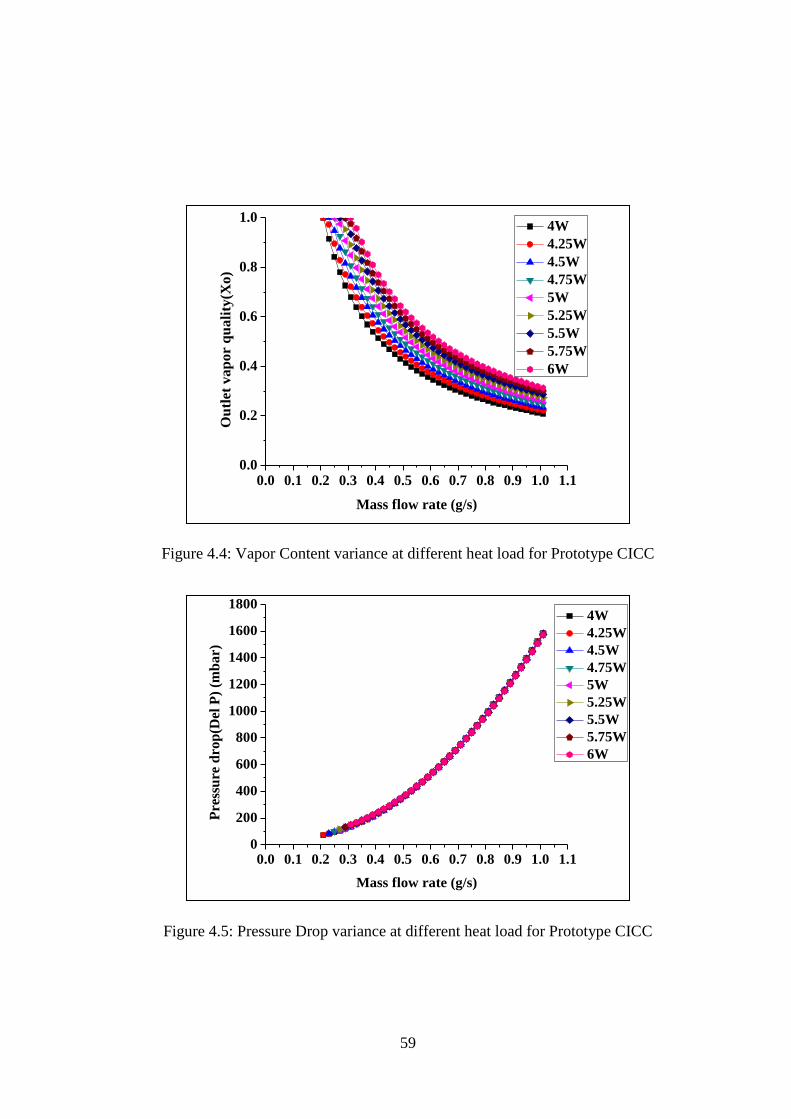
59

Figure 4.4: Vapor Content variance at different heat load for Prototype CICC

Figure 4.5: Pressure Drop variance at different heat load for Prototype CICC

0.0 0.1 0.2 0.3 0.4 0.5 0.6 0.7 0.8 0.9 1.0 1.10.0

0.2

0.4

0.6

0.8

1.0O

utl

et

va

po

r q

ua

lity

(Xo

)


4W

4.25W

4.5W

4.75W

5W

5.25W

5.5W

5.75W

6W

0.0 0.1 0.2 0.3 0.4 0.5 0.6 0.7 0.8 0.9 1.0 1.10

200

400

600

800

1000

1200

1400

1600

1800

Pre

ssu

re d

rop

(Del

P)

(mb

ar)


4W

4.25W

4.5W

4.75W

5W

5.25W

5.5W

5.75W

6W

60

Figure 4.6:Two-phase length variance at different heat load for Prototype-CICC


The pressure drop and quality factor analysis have been carried for a prototype CICC

wound high field superconducting magnet for a number of realistic heat flux and inlet

mass flow rates. The effective temperatures have also been predicted. The analysis may

be useful for future TP flow related experiments in a complex geometry like CICC. The

results also state that as the mass flow rate increases, corresponding pressure drop

increases and hence the vapor quality decreases for a given heat flux. Analyses have

shown results that CICC wound fusion magnets may be operated in the TP flow of helium

under certain operational envelopes as discussed. The TP cooling of CICC do get into

risks of flow choking and thermo-acrostic instabilities possibilities, but ensuring single

phase sub-cooling at the inlet these possibilities in practice could be reduced significantly

or even eliminated for certain heat flux and operating parameters. Even though the TP

cooling and its thermo-hydraulics are complex in nature to realize, by using the

0.2 0.4 0.6 0.8 1.00

5

10

15

20

25

30

35

40

45

Tw

o P

ha

se S

ecti

on

(m

)


4W

4.25W

4.5W

4.75W

5W

5.25W

5.5W

5.75W

6W

61

prescriptions discussed above, reasonable predictions of these essential quantities of the

flow scheme are feasible (effective temperature, pressure drop and vapor quality). The

obvious advantage of the TP cooling as against the single-phase cooling is the reduced

requirements of the mass flow rates. Thus, in a cryogenic system, the stringent

requirements of a cold circulator and its associated heat flux budget may be eliminated or

at least reduced. Further, the resulting cooling scheme becomes simpler. These

information may be helpful in practical operations of TP cooled magnets in future.

63

CHAPTER- V

5. Experimental studies of two-

phase flow pattern

visualization in horizontal LN2

flow

5.1 Motivation

5.2 Various two phase flow regime maps relevant for

horizontal flow






5.3.5 Data acquisition system




64

5.1 Motivation

The TP flow is primarily attributed to the turbulent mixing of TP, compressible nature of

the gas phase and other factors like mass flow rates of individual phases, fluid thermo-

physical properties, channel geometry and orientation etc. The present study is an

experimental attempt to quantify and visualize the flow patterns of two TP nitrogen flows

in a horizontal configuration. The cryogenic TP flow is of significant practical interest

such as in the transfer lines where the quality of the mixture changes continuously due to

heat load and frictional dissipation in the flow passage. Due to dual nature of the phases,

it is not possible to measure accurately fluid flow rate. Hence, proper modeling and

experimentation are required, whenever TP flows are used in cryogenic systems in order

to ensure proper functional performance.

A laboratory scale Liquid Nitrogen (LN2) TP visualization experimental facility has been

custom designed, fabricated and realized to study the flow structure in horizontal TP flow

involving cryogenic fluid [44]. TP flow is classified according to the phase distributions

or "flow patterns" or "regimes" [44]-[49]. For various LN2 flow, vapor quality is

estimated for fixed Gaseous Nitrogen (GN2) flow. The facility incorporates Pyrex

viewing section from which the flow structure or patterns is observed and recorded using

a digital imaging device. Temperature and pressure measurements are recorded from

several sensors throughout the facility to monitor the flow conditions. Visualizations of

the flow structure with cryogen have revealed the presence of several transitions

depending on the initial conditions. This experiment on TP flow characteristics, with

liquid nitrogen flowing through a horizontal transfer line, has shown up several flow

structures. These data will be used in future research towards the development of a

prototype void sensor capable of measuring the liquid hold up involving cryogenic TP

65

flows. Results presented in this chapter have been published in a peer reviewed journal

[50].

5.2 Various two-phase flow regime maps relevant

to horizontal flow

The TP flows are characterized by their flow regimes, which describe the arrangements in

the flow and the relative fractions of the liquid and vapor in the flow. There are numerous

flow regime maps that have been developed for horizontal as well as vertical flows. In

this section, the maps described are mostly used for horizontal flow studies.

The Baker map

The flow regime map proposed by Baker [51] in 1954. Baker plotted the observed flow

pattern using air-water and steam-water as a working fluid by using an empirical

correlation method. The map plotted comprises the liquid mass flux (GL) versus gas mass

flux (Gg) as shown in Figure 5.1. The transition lines were drawn as per the observed flow

patterns in that particular area. For TP flow with fluids other than air-water and steam-

water, fluid property correction factors were introduced in the map. Thus, the coordinates

of the map are modified by the factors λ andψ, as given in equation 5.1 and 5.2. The new

coordinates of the map become GLᴪ versus Ggλ.

λ = [(ρg

ρa) (

ρL

ρwa)]

0.5

(5.1)

ψ = (σwa

σ) [(

μL

μwa) (

ρwa

ρL)

2

]

13⁄

(5.2)

𝜌 = density of the respective fluid

μ = viscosity of the respective fluid

66

σ = surface tension between the phases

σwa = surface tension between water and air

Figure 5.1: The Baker flow regime map

[Image Source: Appl. Mech. Rev 61(5), 050802 (Jul 30, 2008) ]

Where, the subscripts g, L, a, and wa represent the gas, the liquid, air, and water

respectively.

For cryogenic fluids [3], this map has been used and some success is achieved. However,

the drawback of this map is that variations in pipe diameter or orientation are not taken

into account. Variations in these parameters were shown by Taitel and Dukler [52].

The Taitel and Dukler map

The Taitel and Dukler [52] map, developed in 1976, is the most widely used flow pattern

map for horizontal TP flow. In this map it is assumed that the flow initially exists in the

stratified regime and other flow regimes are formed subsequently. The horizontal

http://appliedmechanicsreviews.asmedigitalcollection.asme.org/article.aspx?articleid=1399061

67

coordinate of the map is the Lockhart–Martinelli parameter (1949). The vertical

coordinates of the map are K on the left hand side and T or F on the right-hand side as

shown in Figure 5.2. They are defined as equation 5.3 and 5.4:

Xtt2 =

|(dP dx⁄ )Ls |

|(dP dx⁄ )gs |

(5.3)

Y =(ρL−ρg)gsinγ

|(dP dx⁄ )gs |

(5.4)

Where the subscripts L and g denote the liquid and gas phases respectively.

|(dP dx⁄ )s| = pressure drop of one phase based on the mass fraction of that phase

g = gravitational acceleration

γ = angle of inclination of the pipe

Xtt = the Martinelli parameter

Y = relative forces acting on the liquid due to gravity and pressure gradient .

F = √ρg

(ρL−ρg)

ugs

√Dgcosγ (5.5)

F = Froude number modified by the density ratio

𝐷 = diameter of the pipe

u = velocity of the respective phase

s = superficial velocity for single fluid flow

K2 = F2Rels (5.6)

T = [|(dP dx⁄ )l

s|

(ρl−ρggcosγ)]

1

2 (5.7)

68

Figure 5.2: The Taitel and Dukler flow regime map


T is the ratio of the turbulent force to the gravity force, as given by equation 5.7, This

map was the first map in which the pipe diameter, as well as the pipe orientation and the

fluid properties dependence of flow regime were included. The drawback of this map is

that the phase change is not taken into consideration and it has not been calibrated with a

large data set till date.

The Wojtan et al. map

The Wojtan et al. [53] map is the modified version of the map given by Kattan et al. [54]

for horizontal flow which eliminates all iterative steps. Kattan et al. [54] used two

refrigerants and he found that his data was in agreement with Steiner map [55] more than

any other previously used maps. However, use of the Steiner map was difficult because in

order to determine flow pattern, complex evaluation of the five different parameters is

required. So, the axes of Steiner map were converted to simpler parameters i.e mass flux,

G, versus vapor quality, x by Wojtan as shown in Figure 5.3.


69

Figure 5.3: The Wojtan et al. flow regime map


The transition curves were empirically modified to improve accuracy and then predictions

could match experimental observations. Wojtan et al. [53] describes the details of the map

construction in his work.



Design of an experimental system aimed at visualizing the TP flow regimes and flow

patterns must be appropriately optimized by certain physical parameters. These

parameters are such as operating pressure, system limitations such as dimensions of the

process tube, the dimension of the measurement probe and the design constraints of the

heat exchanger etc. For these experiments, the LN2 supply source has been a 50-litre

cryostat with an allowable operational pressure head of 500 mbar. This pressure


70

limitation has been one of the prime drivers behind designing the experiment. The

variation of flow pattern as a function of the mass flow during cool down is observed and

recorded. The quality is estimated by measuring mass flow of gas and total flow using

venture flow meters separately. The void fraction as a function of vapor quality and the

flow pattern is predicted using various empirical correlations. The flow regime is

determined from void fraction and flow pattern for the given quality.

Table 5.1: Dimensions of the Test section and heat exchanger

Process Line Outer Jacket Heater exchanger

Pyrex glass

L= 1 m

I.D=9 mm

O.D=12 mm

Pyrex glass

L= 1 m

I.D=25 mm

O.D=28 mm

L=1.5 m

Material= Cu

I.D= 10mm

The Pyrex glass process tube and vacuum jacket dimensions are determined considering

operating pressure, required experimental vacuum and transparency for visualization of

the experiment setup. The interconnection of glass to metal flanges is designed so as to

ensure leak tightness at cold temperature. The test section length is kept 1000 mm and

flow pattern is recorded at different locations along the flow path. The heat exchanger at

the end of the test section is installed to convert TP liquid nitrogen to single phase

nitrogen gas. The dimensions of the test section and heat exchanger are listed in Table 5.1.

Thereafter, the Venturi flow meter measures the total mass flow rate. The heat exchanger

is made up of copper for better heat transfer. This also contributes into the pressure drop

as per mass flow rate in the system. The heat exchanger dimensions are optimized as per

mass flow rate and operating conditions.

71


The experimental setup schematic to study the TP phenomena flow structure is illustrated

in Figure 5.4.

Liquid nitrogen is considered as the working fluid in this experimental set-up. The liquid

nitrogen is stored in high-pressure vacuum jacketed cryostat (at 1500kPa). The LN2 flow

is effected by pressurizing the cryostat with nitrogen gas from a cylinder. Once the fluid

exits the tank, it is directed through the facility. The interconnections are thermally

insulated. Upon entering the facility, the cryogen flow passes through a vacuum jacketed

Pyrex glass section (I.D. 9 mm, O.D. 12 mm, approximate thermal conductivity of 1.005

W/m-K and specific heat of 0.75 kJ/kg-K and emissivity of 0.92). At the inlet, there is a

mixing section, where gas nitrogen is mixed with liquid nitrogen in a controlled pre-

determined manner. The absolute pressure, temperature and the mass flow rate of the

input gases are being measured by Keller make pressure transducer, PT-100 temperature

sensors, and a Venturi meter respectively. The flow structure is captured via a digital

camera with the appropriate image capturing software. The nitrogen then flows through

the heat exchanger section of the test setup to convert liquid nitrogen to vapor at the exit

of the Pyrex test section so as to measure the mass flow rate. A cryogenic manual control

valve is located after the heat transfer section to control the flow. The remaining liquid

nitrogen is converted to room temperature gas nitrogen before entering the flow meter.

Then, the GN2 is vented out into the atmosphere.

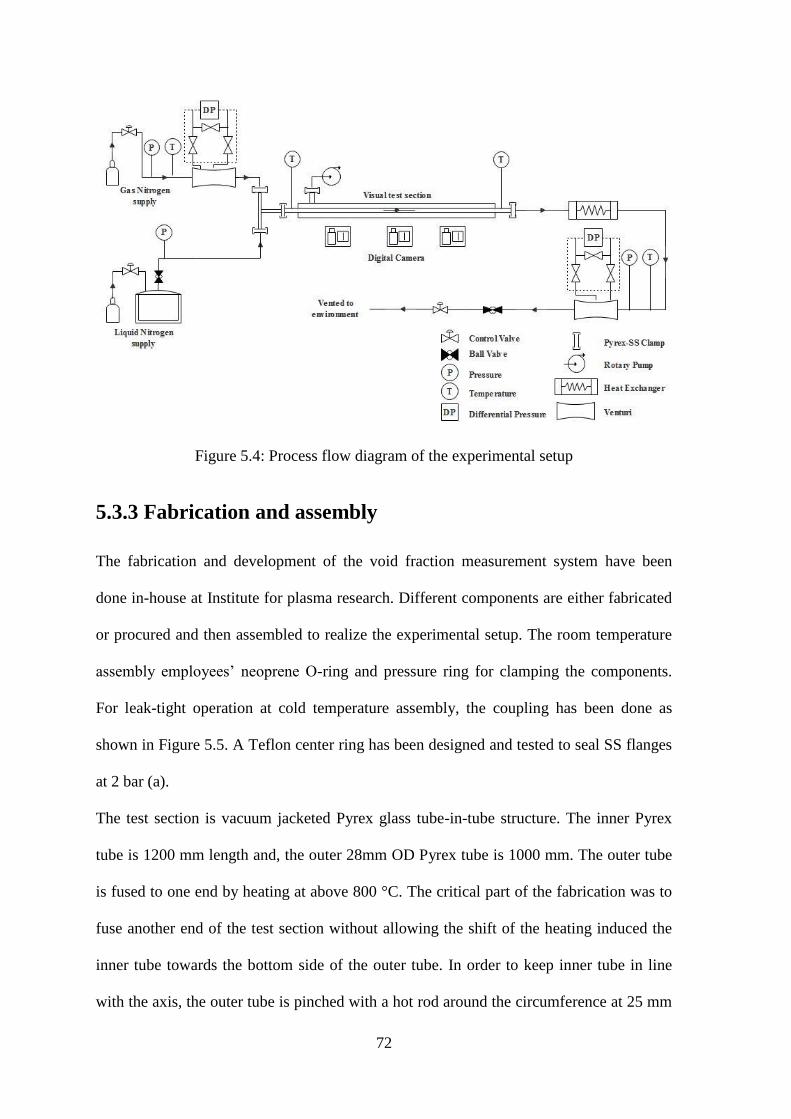
72

Figure 5.4: Process flow diagram of the experimental setup


The fabrication and development of the void fraction measurement system have been

done in-house at Institute for plasma research. Different components are either fabricated

or procured and then assembled to realize the experimental setup. The room temperature

assembly employees’ neoprene O-ring and pressure ring for clamping the components.

For leak-tight operation at cold temperature assembly, the coupling has been done as

shown in Figure 5.5. A Teflon center ring has been designed and tested to seal SS flanges

at 2 bar (a).

The test section is vacuum jacketed Pyrex glass tube-in-tube structure. The inner Pyrex

tube is 1200 mm length and, the outer 28mm OD Pyrex tube is 1000 mm. The outer tube

is fused to one end by heating at above 800 °C. The critical part of the fabrication was to

fuse another end of the test section without allowing the shift of the heating induced the

inner tube towards the bottom side of the outer tube. In order to keep inner tube in line

with the axis, the outer tube is pinched with a hot rod around the circumference at 25 mm

73

from the fusing end. The inner tube is rested on this pinched structure and the outer tube

is heated to fuse with the inner rod for the vacuum tightness.

Figure 5.5: Coupling schematic

The vacuum is maintained at 10-3

mbar during experimental runs. Inlet and return glass

port with 16 KF flange is fused in process tube. A glass vacuum port is fabricated on the

outer vacuum tube for evacuation. The complete test setup is leak tested to ensure the leak

tightness. The leak test has been performed at room temperature and at cold temperature.

During the thermal cycle, the leak rates are monitored. The leak test is done in vacuum

mode using a leak detector and helium gas. In vacuum mode, the line is evacuated and

helium is sprayed and leak rate is measured.

The temperature sensors are mounted on the process line. The temperature sensor wires

are thermally anchored. After complete assembly of the test section, a global leak test is

done at room temperature and again at cold temperature. The heat exchanger is coupled to

the test section using similar assembly as shown in Figure 5.5. The complete setup is

assembled and each joint is leak tested. The acceptable leak rate in sniffer mode is 10-6

mbar lit/sec and in vacuum mode is 10-9

mbar lit/sec. The electrical continuity of sensors

is checked before commissioning the experiment setup.

74


The sensors and diagnostics used in the experimental setup are described in section 2.2.4

of chapter 2.


Data acquisition has been done with 8 channel Masibus scanner, which provides front

panel display of the process values. The scanner is connected with process analog input

values at input channels and relay terminals. Channels are selected as per our process

variable requirements. As per the requirement, one analog channel is selected and

necessary settings are done for communication with Modbus, desktop display, SCADA,

and Scanner.

The Output voltage 𝑉𝑜 of the electronic circuit is connected with the analog input channel

of the scanner. The analog input channel number, upper, lower voltage range, baud rate,

parity bit etc. is programmed manually. A/D conversion process is done in the scanner

and it gives proportional count values for communication with SCADA. Output of the

scanner (counts) is communicated to the PC via Modbus RS485 interface. RS485 is

required for communication configuration. Output of RS485 Modbus is connected with

serial communication to PC as given in Figure 5.6. Each process value from the scanner

is addressed with Modbus formatting.

SCADA system is used to show the actual process and instrumentation. A graphical user

interface (GUI) has been developed on desktop PC with Citect SCADA. Tags for process

values are developed with Modbus protocol in addressing formatting. The data logging

have been done for each process variable in the interval of 0.5 seconds in real time. A

historical trend screen has been developed for the study and analyzing of real-time data.

This whole work is carried out indigenously in the lab.

75

Figure 5.6: Data acquisition system block diagram


Experiments have been carried out in the following manner:

a. The data acquisition program is activated to initiate recording of the data.

b. The Digital imaging device is activated so that it may begin capturing the flow

structure.

c. The heater of 1.5 kW of the heat exchanger is switched on so that LN2 may vaporize

before entering Venturi flow meter.

d. The nitrogen cryostat connected to the setup is opened and the data acquisition and

digital camera are started.

e. Gas nitrogen is flown through the setup and major connections are checked at room

temperature.

f. Sensors, vacuum and flow rate are monitored.

g. Liquid nitrogen is allowed to flow through the facility.

h. The temperature, pressure, and mass flow rate measurements are recorded.

i. The flow patterns images are recorded.

j. The above steps are repeated with the throttling valve in different positions

76

k. At fixed gas flow rate, liquid nitrogen flow is increased and this step is repeated for

variously fixed gas mass flow rate.


For the calibration of pressure and flow transmitter and its DAQ, forced flow GN2 is

passed through the facility at the beginning. Experimental task was to find the relation

between Inlet pressure and GN2 mass flow rate in the range of 0-1 g/s. Similarly, LN2 was

forced flow by pressurizing LN2 storage cryostat to know the range of mass flow rates.

The liquid mass flow is varied within experimental limitations.

Flow pattern observed during cool-down at 1.1 bar (a) pressure

and <ṁ> ~ 1 g/s

The cool-down of the visualization section is done with low mass flow rate and flow

pattern is recorded by the digital camera. Figure 5.7 illustrates various flow pattern

observed during cool down of the testing section at mass flow <ṁ> ~ 1 g/s.

a). Evaporation of liquid b). The film of LN2 as cool down progresses

c). Liquid flow front as the surface cools d d). Liquid flow sustains after cool down

77

e). Wavy flow f). Stratified flow

Figure 5.7: Flow pattern observed at 1.1 bar (a) pressure and <ṁ> ~ 1 g/s

The testing section is at room temperature hence LN2 vaporizes as the cooldown

progresses (Figure 5.7 a). As the temperature of testing section decreases, LN2 is

observed to sustain on the lower part of the test section and film boiling is observed as

flow progresses (Figure 5.7 b-d). After this point, LN2 sustains in the lower portion of the

test section and the wavy pattern is observed. When complete cooldown is done stratified

flow is observed at the given mass flow rate (Figure 5.7 e-f).

Flow pattern observed during cool down at 1.2 bar (a) pressure

and <ṁ>~ 2 g/s

The complete cooldown of the test section is done. In order to explore the flow pattern on

even higher mass flow rate, the LN2 is forced flow through the test section at inlet

pressure of 1.2 bar (a) at the mass flow rate of nearly 2 g/s. The flow patterns observed

are illustrated in Figure 5.8.

a). Slug flow b). Stratified wavy flow

78

c). Wavy flow d). Slug flow

e). Wavy flow f). Stratified flow

Figure 5.8: Flow pattern observed at 1.2 bar (a) pressure and <ṁ> ~ 2 g/s

When the mass flow increases, there is a sudden flow of LN2 is observed. Thereafter,

there is a smooth wavy or wavy flow pattern observed. These patterns are repeated when

the mass flow is kept constant at these values. Figure 5.8illustrates the sequence of the

pattern observed at an inlet pressure of 1.2 bar and mass flow of 2 g/s.

Flow pattern observed during cool-down at 1.3 bar (a) pressure

and <ṁ> ~ 2.5 g/s

a). Stratified flow b). Stratified wavy flow

79

c). Slug flow d). Wavy flow

e). Plug flow f). Plug flow

Figure 5.9: Flow pattern observed at 1.3 bar (a) pressure and <ṁ> ~ 2.5 g/s

On further increasing Inlet pressure to 1.3 bar (a), mass flow obtained was nearly 2.5 g/s

and the flow pattern observed are shown in Figure 5.9. The liquid could be seen more in

the horizontal test section and various flow patterns could be observed under the same

condition. It is observed that when inlet pressure is increased, mass flow rate of liquid in

increased. A sudden increase in flow follows the stratified and stratified wavy pattern and

sometimes slugs are observed after wavy flow. These patterns are repeated when flow

conditions are maintained the same.

Flow pattern observed during cooldown at 1.5 bar (a) pressure

and <ṁ> ~ 3.5 g/s

a). Stratified wavy b). Stratified wavy

80

c). Wavy flow d). Stratified flow

e). Plug flow f). Pure liquid

g). Wavy flow h). Wavy flow

g). Plug flow h). Plug flow

i). Slug flow j). Stratified flow

Figure 5.10: Flow pattern observed at 1.5 bar (a) pressure and <ṁ> ~ 3.5 g/s

81

Further inlet pressure is increased to a maximum of 1.5 bar (a) (safety valve of cryostat

opens above 1.5 bar (a)) and the mass flow obtained is 3.5 g/s. At 1.5 bar (a) inlet

pressure different repetitive flow pattern observed is depicted in Figure 5.10.

As the pressure is further increased, the velocity of the fluid is increased and, due to

gravity liquid tends to settle on the lower portion of the testing section. This results in

observing stratified flow pattern in most of the cases (Figure 5.10). Due to increase in

velocity, wavy pattern is observed. For the given cross-section and high mass flow rate

sometimes plug and slug flow patterns are also observed in the test section. These flow

patterns are repetitive at the given inlet condition. As there is a heat exchanger after

testing section, the LN2 is converted to GN2 for the flow measurement, there are some

fluctuations in mass flow rate and accordingly, it is reflected in the flow pattern.

Maximum observed flow pattern in these conations is stratified, wavy and slug flow.

At constant GN2 mass flow rate vary the LN2 mass flow rate

After observing the flow pattern of LN2 in the test section, GN2 and LN2 are mixed and

are forced flown together into the test section. The resulting flow patterns are then

investigated parametrically as a function of input conditions. In all these experiments,

prior to introducing the TP flow into the test section, the GN2 is first mixed with LN2 in

the mixing section in order to stabilize the flow. Subsequently, the TP flow pattern is

studied in the test section.

a). Slug flow b). Slug flow

82

c). Stratified flow d). Stratified wavy flow

e). Stratified wavy flow f). Wavy flow

Figure 5.11: Experimentally observed flow pattern transitions for the fixed gas flow and

increasing liquid mass flow rate

Vapor void is predicted using various model/correlations listed in Table 1.2. Using

various well established TP maps, the experimental data have been plotted and compared

to the flow patterns as observed and recorded with the digital camera. In the experiment

GN2 mass flow ( ṁg ) is measured using one Venturi meter and total mass flow (ṁT ) is

measured using a Venturi at the outlet of the facility. Liquid mass flow ( ṁL) is estimated

by subtracting GN2 mass flow from total flow rate. By keeping GN2 flow rate constant,

the LN2 flow rate is gradually increased and the resulting flow patterns are then observed.

The quality, void and pattern mapping are then derived and analyzed from the input

parameters and measured data. Figure 5.12 summarizes the experimental data recorded

for various fixed GN2 flow rates.

Gas mass flow is varied from 0.45 g/s to 1.07 g/s for a number of fixed liquid flow rates.

Similarly, for a number of fixed gas flow rates, the liquid flow rate is varied. In all these

set of experiments, the input conditions and all the observations are recorded. Figure 5.11

represents the flow pattern observed for the case of the fixed GN2 flow of 0.45 g/s and

83

1.07 g/s. The Figure 5.11 illustrates a stratified and wavy pattern in most of the

experimental cases.

Figure 5.12: Variation of the total flow rate by varying LN2 flow rate at the constant GN2

flow

Case 1): ṁ𝒈=0.45 g/s, ṁ𝑳=1.7-2.6 g/s, 𝒙=0.15-0.20, 𝑨𝒇=63.62 mm2

The GN2 mass flow is kept constant at 0.45 g/s and LN2 mass flow is varied by

pressurizing cryostat. The obtained LN2 mass flow is 1.7-2.6 g/s. Quality is estimated by

taking the ratio of mass flow of GN2 upon total mass flow, which comes out to be 15 %-

20%. Flow pattern observed are stratified, wavy, and stratified wavy. The void fraction is

predicted using various empirical TP correlations and plot is shown in Figure 5.13. Table

5.2 gives the predicted void fraction range as a function of vapor quality using various

correlations.

84

Table 5.2: Predicted void using correlations for GN2 flow =0.45 g/s

Void correlation Predicted Void range

ṁ𝒈=0.45 g/s Homogeneous 0.92-0.94

𝒙=0.15-0.20 Lockhart and Martinelli 0.90-0.92

ṁ𝑳=1.7-2.6 g/s Fauske 0.80-0.85

Lenvi 0.85-0.89

Figure 5.13: Prediction of void using correlations for GN2 flow =0.45 g/s

Case 2): ṁ𝒈 =0.69 g/s, ṁ𝑳 =1.64-2.21 g/s, 𝒙 =0.23-0.30, 𝑨𝒇 =63.62

mm2


pressurizing cryostat. The obtained LN2 mass flow is 1.64-2.21 g/s. Quality is estimated

by taking the ratio of mass flow of GN2 upon total mass flow, which comes out to be

23%-30%. Flow pattern observed are stratified and wavy. The void fraction is predicted

using various empirical TP correlations and plot is shown in Figure 5.14. Table 5.3 gives

the predicted void fraction range as a function of vapor quality using various correlations.


85


ṁ𝑔=0.69 g/s Homogeneous 0.95-0.96

𝑥=0.23-0.30 Lockhart and Martinelli 0.93-0.94

ṁ𝐿=1.64-2.21 g/s Fauske 0.87-0.90

Lenvi 0.91-0.93


Case 3): ṁ𝒈=0.84 g/s, ṁ𝑳=1.4-2 g/s, 𝒙=0.30-0.36, 𝑨𝒇=63.62 mm2


pressurizing cryostat. The obtained LN2 mass flow is 1.4-2 g/s. Quality is estimated by


36%. Flow pattern observed are stratified and wavy. The void fraction is predicted using

various empirical TP correlations and plot is shown in Figure 5.15.

Table 5.4 gives the predicted void fraction range as a function of vapor quality using

various correlations.

86





ṁ𝐿=1.4-2 g/s Fauske 0.90-0.92

Lenvi 0.93-0.95


Case 4): ṁ𝒈=0.97 g/s, ṁ𝑳=1.3-2 g/s, 𝒙=0.32-0.43, 𝑨𝒇=63.62 mm2


pressurizing cryostat. The obtained LN2 mass flow is 1.3-2 g/s. Quality is estimated by


43%. Flow pattern observed are stratified and wavy. The void fraction is predicted using

various empirical TP correlations and plot is shown in Figure 5.16. Table 5.5 gives the

predicted void fraction range as a function of vapor quality using various correlations.

87





ṁ𝐿=1.3-2 g/s Fauske 0.91-0.94

Lenvi 0.93-0.96


Case 5): ṁ𝒈 =1.07 g/s, ṁ𝑳 =1.18-1.96 g/s, 𝒙 =0.35-0.48, 𝑨𝒇 =63.62

mm2


pressurizing cryostat. The obtained LN2 mass flow is 1.18-1.96 g/s. Quality is estimated

by taking the ratio of mass flow of GN2 upon total mass flow, which comes out to be

35 %-48%. Flow pattern observed are stratified and wavy. The void fraction is predicted

using various empirical TP correlations and plot is shown in Figure 5.17. Table 5.6 gives

the predicted void fraction range as a function of vapor quality using various correlations.

88



ṁg=1.07 g/s Homogeneous 0.97-0.98

x=0.35-0.48 Lockhart and Martinelli 0.95-0.96

ṁL=1.18-1.96 g/s Fauske 0.92-0.95

Lenvi 0.94-0.96

Figure 5.17: Prediction of a void using correlations for GN2 flow =1.07 g/s

Vapor quality estimation

Vapor quality is estimated by taking ratio gas mass flow and total mass flow rate. The gas

flow rate is constant; quality varies as liquid flow rate varies. Figure 5.18 represent

experimentally obtained vapor quality by varying LN2 flow.

Vapor void fraction prediction

Void fraction gives the information on the liquid holdup in TP flow at certain inlet

conditions. Vapor void fraction is predicted using the TP flow void fraction empirical

correlations listed in Table 1.2. Figure 5.19illustrates the relationship between void and

quality by homogeneous void correlations [7]. Similarly, Figure 5.20 represent void

89

fraction variation using Lockhart and Martinelli correlation[8], Figure 5.21 represent void

fraction variation using Fauske correlation [9] and Figure 5.22 shows the void fraction

variation using Lenvi correlation [10]. Predicted void fraction range using various

correlations has been listed in Table 5.7.

Table 5.7: Void fraction and its variation using void correlation


x=0.15-0.48 Homogeneous 0.92-0.98

ṁg=0.45 g/s to 1.07 g/s Lockhart and Martinelli 0.90-0.96

Fauske 0.80-0.95

Lenvi 0.86-0.96

These predictions through various models motivate at developing a sensor which can

measure the void fraction experimentally. The measurement of quality is difficult, as for

the measurement either both phases are separated completely or evaporated. The

experimental measurement will also benchmark the TP correlation that could be

considered for the cryogenic TP flow. The void fraction measurement system is described

in chapter 6.

90

Figure 5.18: Variation of quality on increasing LN2 mass flow rate at a fixed GN2 flow

rate

Figure 5.19: Prediction of a void fraction as a function of vapor quality using

homogeneous model

91

Figure 5.20: Prediction of a void fraction as a function of quality using Lockhart-

Martinelli model

Figure 5.21: Prediction of a void fraction as a function of vapor quality using Fauske

model

92

Figure 5.22: Prediction of a void fraction as a function of vapor quality using Lenvi’s

model

Flow Regimes

To study the hydrodynamics of two phase flow it is essential to know the distribution of

phases in the flow. A reliable flow regime transition map is not yet developed for the

cryogenic two phase flow. Experiments have been carried out and the flow regime

transitions in a horizontal test section have been observed and recorded using liquid

nitrogen. The observations have been compared with the well-established regime maps

described in section 5.2.

The flow patterns obtained experimentally for horizontal LN2 flow have been compared

with the three well-known flow pattern maps viz.by Baker [51], Taitel and Dukler [52],

and Wojtan et al. [53].

In Figure 5.23 the experimental data is compared with the Baker map. It is observed that

the experimental data have correlated well, and the experimentally found flow regime lies

in the stratified/wavy region in the Baker’s map. This map is based on a simple flow

model and therefore, is not able to predict mixed flow patterns. Whereas, the flow regime

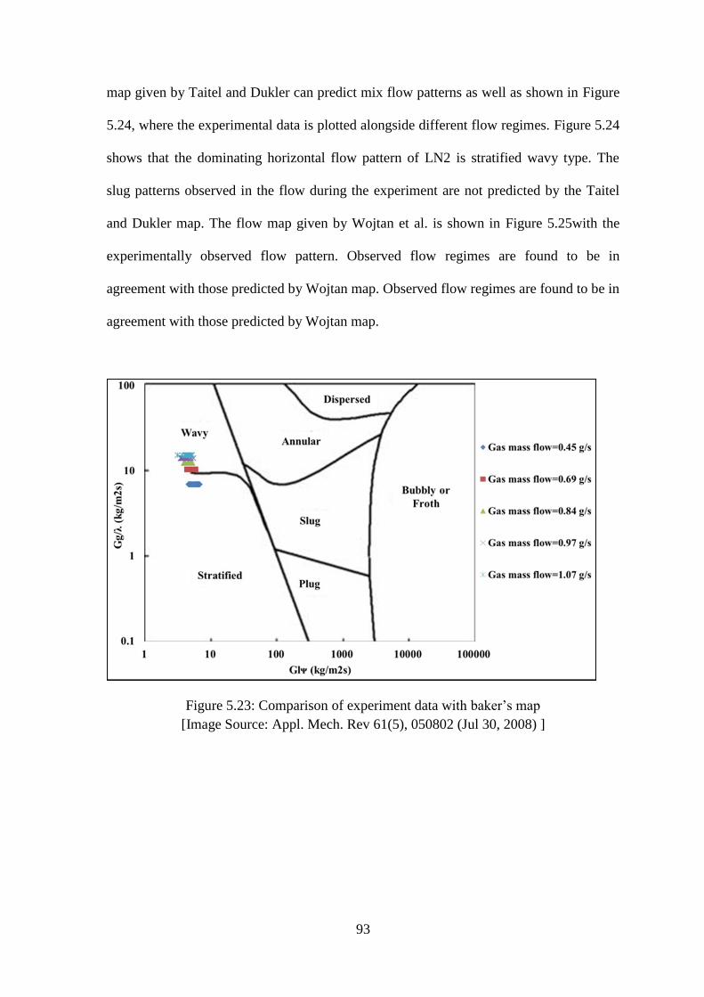
93

map given by Taitel and Dukler can predict mix flow patterns as well as shown in Figure

5.24, where the experimental data is plotted alongside different flow regimes. Figure 5.24

shows that the dominating horizontal flow pattern of LN2 is stratified wavy type. The

slug patterns observed in the flow during the experiment are not predicted by the Taitel

and Dukler map. The flow map given by Wojtan et al. is shown in Figure 5.25with the

experimentally observed flow pattern. Observed flow regimes are found to be in

agreement with those predicted by Wojtan map. Observed flow regimes are found to be in

agreement with those predicted by Wojtan map.

Figure 5.23: Comparison of experiment data with baker’s map



94

Figure 5.24: Comparison of experiment data with Taitel and Dukler map


Figure 5.25: Comparison of experiment data with Wojtan map




95


Experiments have been carried out for mass fluxes that range from 16 to 55 kg/m2-s, and

vapor qualities vary from 0.15 to 0.48. The flow pattern and corresponding flow

structures observed during this investigation are shown in Figure 5.7-Figure 5.11. A film

boiling is observed when the liquid nitrogen first enters at the entrance to the test section.

This film boiling front produces a rapid evaporation traveling down the test section. As

the temperature of surface cools down, liquid droplets sustain at the lower surface. As the

mass flux is increased, a stratified wavy structure is observed. A stratified-wavy flow

pattern is observed at low mass fluxes usually below 30 kg/m2-s. A thin liquid layer is

seen to be flowing through the test section. As the test section cools down, the flow

pattern transits from stratified-wavy to the plug and slug flow pattern. At higher mass

fluxes usually above 30 kg/m2-s, the dominating flow regime observed was stratified

wavy but, there were transition in plug and slug regime. LN2 mass flow is varied by

keeping GN2 flow rate constant and the mixture flows through the testing section from

mixing section. The observed flow regime is stratified and wavy for given input

parameters. The vapor volume fraction has been computed using the mass flow rates of

GN2 and LN2. The computed vapor quality profile is illustrated in Figure 5.18. The

current research offers a much greater detailed description of the cool-down sequence and

flow regimes involving TP nitrogen in horizontal flow configurations. In early phases

when pulses of liquid, which is flashed into gas, a film boiling is observed to occur. The

vapor volume fraction and quality curves as observed in experiments appear to be in

general agreement with the visually observed flow pattern.

This work is a maiden attempt in compiling a database through experiments of the flow

structures, the mass flow rates, the vapor quality and predicted void fraction in various

flow regimes involving TP nitrogen flow in a horizontal configuration. LN2 and GN2 are

96

forced flow separately through a test section as a part of calibration of the experimental

system. Thereafter, by varying liquid Nitrogen flow rates with the constant gas flow, the

variation of a void fraction as a function of a quality factor has been investigated. Void

fraction has been successfully predicted for a range of experimental quality factor using

Lockhart-Martinelli, Fauske, Lenvi and Homogeneous TP flow models. Using standard

flow regime models; Backer’s regime map, The Taitel, The Dukler and Wojtan flow

regime map have been analyzed. These have been compared with the flow visualization

using fast Digital camera. Different flow patterns have been realized using different

process parameters leading to a comprehensive investigation of TP nitrogen flow in a

horizontal configuration. This work provides a critical database that will be helpful

towards the development and improvement of models and correlations. The experimental

database could also be used in the development of an appropriate void sensor or quality

meter.

97

CHAPTER - VI

6. Experimental design of void

fraction measurement system

for horizontal LN2 two-phase

flow

6.1 Motivation

6.2 Importance of void fraction measurement

6.3 Techniques of void fraction measurement

6.4 Void fraction measurement system





6.4.5 Development of a void measurement circuit

6.4.5.1 Physical principle and design drivers

6.4.5.2 Electronics and signal conditioning

6.4.5.3 Calibration details





98

6.1 Motivation

In cryogenic applications, accurate information and measurements of certain critical

parameters are mandatory. In a single phase cryogenic flow, flow rate or flow velocity as

well as the thermodynamic state parameters such as density` ρ’, viscosity` η’, entropy `S’

and enthalpy `h’ etc. determined by pressure `P’, and temperature `T’ are important. In

`TP’ cryogenic flows the `latent heat of vaporization’ due to heat-in-leaks of the system is

often observed. In the case of TP flow, the thermodynamic properties associated with the

flow are not determined by P and T only. Information of `vapor quality’, the ratio of

`vapor flow rate’ to the `total flow rate and `vapor void’ the ratio of the cross-sections of

respective phases are critically important.

The quality of the TP mixture changes continuously due to `heat load’ acting on it, as

well as from frictional heating along the flow path. The thermodynamic characteristics i.e.

enthalpy and entropy in TP flow are determined as `mean flow values’;

hm = hgx + hl(1 − x) (6.1)

Sm = Sgx + Sl(1 − x) (6.2)

and as `mean volume characteristics’ such as density and viscosity, represented as

equation 3.3 and 3.4.

The mass flow rate of the TP mixture is extremely difficult to be measured. However,

they can be calculated from the experimental data if, the pressure drop ` ∆P′ of the

measuring device, quality` x’, and the physical properties of phases are known. On the

contrary, measurement of `x’ is very challenging without the separation of phases or the

complete evaporation of liquid phase. Thus, `void fraction’ is the most vital parameter

towards prediction of any hydrodynamic properties and hence characterizing the TP flow.

The `x’ and `α’ are related to each other with simple correlations. This allows one to

99

determine the thermodynamic characteristics and flow rate of TP mixture. Therefore, the

measurement of void fraction in TP flow phenomena is extremely critical towards flow

characterization. Results presented in this chapter have been published in a peer reviewed

journal [56].

6.2 Importance of void fraction measurement

The void fraction`α’ depends upon several influencing factors. These factors are functions

of the distribution of the phases, the flow rates of the respective phases, the physical

properties of the respective phases and the orientation of flow paths etc. The inlet

composition can be experimentally measured but the void fraction cannot be determined

directly from inlet composition in a flow where heat-in-leaks are present along the

passage of flow.

The void fraction measurements importantly yield a measure of the composition of the TP.

Thus, the estimation of the mixture density, the mixture velocities etc. are feasible. In

industrial applications and practices, the pressure drop in TP scenarios cannot be

evaluated without knowledge of α or liquid hold-up in the system. Therefore, for all

practical cryogenic applications, either an estimation of liquid holdup or an estimation of

void fraction is unavoidable.

6.3 Techniques of void fraction measurement

There exists various void fraction measurement techniques [57]-[69]. Most of them

depend on the variation of average density in TP mixture.

The radiation attenuation method [67] is mostly used for conventional fluid like water.

This method constitutes a radiation source and a detector. The amount of attenuation of

the radiation beam through flowing medium depends on the mixture density or the void

100

fraction in the TP flow. In cryogenic application, this method has also been reported

[67][68]. However, this method has not turned out to be very successful for cryogenic

applications since the amount of attenuation in the flow is much lower than the

attenuation through surrounding cryostat. On the contrary, this method is popularly used

for non-cryogenic fluid TP void measurements.

Similarly, optical methods [58] are used with a source and detector and amount of ray

absorption are measured to determine the void in the flow. This method proves to be

inaccurate and expensive. Electrical resistivity probes have been constructed for

conductive fluid void fraction measurements [57]. Probes are placed across the flow and

change in the voltage drop between these probes measures the void fraction. Cryogens are

nonconductive and also this method is intrusive in the flow. Thus, this method is avoided

in void fraction measuring sensors appropriate for cryogenic fluids.

The void fraction in the TP flow of cryogens can be determined by measuring the

respective dielectric constants and the resultant dielectric constant of TP mixtures.

Further, the dielectric constant of saturated liquid differs from that of the saturated vapor.

Capacitance probes [70]-[75], therefore, can be effectively used towards measuring the

void fraction of the TP mixture. In a practical set-up, the TP mixture is allowed to flow

through the capacitance probe. The overall measured capacitance depends on the

dielectric constant of the mixture and in turn, on its average density. Small changes in

capacitance can be measured with precision measuring techniques. The successes of the

measurements depend on the probe geometry, installation of the probe and electronic

precision and accuracy of the measurements involved. The changes in the dielectric

constant from the liquid phase to complete vapor phase of Helium is 4%. The same is 20%

for Hydrogen, 48% for Oxygen, and 43% for nitrogen. Therefore this method of

measurements could be extended to measuring the void fractions of a spectrum of

101

cryogenic TP mixtures. The advantages of this method are that it is non-intrusive, it has a

quick response, it involves low cost and after all its construction is simple. However, for

helium TP flows, this method may not be very accurate as the change in dielectric

constant from liquid to vapor is only 4%. Thus, in case of helium TP flow Radio

frequency (RF) method may be employed [70]-[72]. Nevertheless, RF-based methods are

complex and expensive. The present work focuses on void measurements of TP Nitrogen

cryogen flow employing very sensitive capacitive probes. The void fraction measurement

system developed for these purposes have been discussed in detail in section 6.4

6.4 Void fraction measurement system


Design of an experimental system aimed at measuring the void fraction must

appropriately optimize certain physical parameters such as operating pressure and system

limitations such as dimensions of the process tube, the dimension of the measurement

probe and the design constraints of the heat exchanger etc. For these experiments, the LN2

supply source has been a 50-litre cryostat with an allowable operational pressure head of

500 mbar. This limitation has been one of the prime drivers behind designing the

experiment. The experimental objectives have been the variation of vapor void as a

function of quality. This will be deduced from the experimental data measuring mass flow

of gas and total flow using venture flow meters.

The process tube and the capacitance probe dimensions have been designed considering

operating pressure, allowable pressure drop and bulkiness of the experimental setup. The

probe is designed such that the flow cross-section of the test section is preserved. The

capacitance of the probe is directly proportional to the length of the capacitor. The length

102

of probe 700 mm has been optimized in such a way that the capacitance is in the 100 pF

range or more. An electronic circuit has been developed aimed at measuring the

capacitance in the range of picoFarad accurately with minimum error. The heat exchanger

contributes to the pressure drop as per mass flow rate in the system. The heat exchanger

dimensions are therefore optimized as per mass flow rate and operating conditions. The

dimension of the test section is listed in Table 6.1.

Table 6.1: Dimensions of the test section

Process Line Outer vacuum

Jacket

Supply section Void sensor

geometry Return section Coupler

SS 304 SS 304 SS 304 Teflon SS304

I.D=9 mm I.R. = 4mm I.D=12.5 mm O.D=36 mm L= 1.5 m

O.D=12 mm O.R. = 6.25 mm O.D=17.15 mm L=80mm I.D=54.76 mm

L=350mm L=700 mm L=400mm O.D=60.3 mm


An experimental setup designed and developed is meant to measure the TP void fraction

in liquid nitrogen flow in a horizontal orientation. For this investigation, liquid nitrogen

has been considered as the working fluid. The schematic layout of the setup is shown in

Figure 6.1. The experiment setup constitutes three sections a) Supply section b) Test

section c) Return section.

The supply section constitutes gaseous nitrogen (GN2) supply, LN2 supply and mixing

section. The GN2 flow is controlled using a manual control valve and mass flow rate is

measured using venture flow meter.LN2 flow is provided by pressurizing LN2 cryostat

Dewar using GN2. The cryostat is equipped with a safety valve set at 1.5bar (a). Thus, the

103

flow potential of liquid nitrogen is limited to 0.5 bar pressure difference. The GN2 and

LN2 are mixed in the `T’ shape mixing section made of SS 304L of length 120 mm. The

flow in mixing section is a homogenous flow before entering test section.

Figure 6.1: Experiment setup process flow diagram

Once the flow exits the storage cryostat and gets mixed with GN2, it is directed to the test

section. The test section is a vacuum jacketed setup made of SS304L. It constitutes supply

process line, void fraction probe, and return process line. The process line has the

dimensions of I.D. of 9 mm, the thickness of 1.5 mm and length of 350 mm. The TP

mixture travels through process line before entering void fraction probe. Void fraction

probe is a coaxial capacitor made of stainless steel. The probe is 700 mm long with 80

mm Teflon coupler on both ends. Both couplers are sealed with stycast material to

maintain leak tightness at room temperature as well as at LN2 temperature. The

dimensions of the probe are given in Table 6.1. The area of the annular region between

electrodes is preserved and is nearly equal to that of supply process line. This eliminates

any changes in the void fraction and pressure drop due to change in flow area. The

104

change in the nitrogen density due to TP flow results in the change of the dielectric

constant of the nitrogen flowing inside the probe. This results in the change of the

capacitance of the probe. This change will be detected by a novel electronic circuit as

shown in Figure 6.3. The TP mixture from the probe is then directed to the return process

line made of SS 304L. A flexible leak tight bellow is placed at the end of process line to

compensate for any thermal stress when the line is cooled from room temperature to

cryogenic temperature. The complete test section is vacuum jacketed and the vacuum is

maintained at ~ 10-3

mbar. The process line and the probe are shielded from thermal

radiation by multi-layer insulation.

The experimental setup return section comprises a heat exchanger. This heat exchanger

converts nitrogen TP mixture to room temperature gas. The heat exchanger is made up of

copper and is dipped in a pool of water that is heated using 1.5 kW heater. The heat

exchanger converts TP nitrogen to room temperature nitrogen gas. The room temperature

GN2 is then directed to the Venture flow meter to measure the total mass flow rate. A

manual control valve installed at this location controls the mass flow rate. The nitrogen

during the experiment is then vented to atmosphere. The fabrication and the assembly of

the experiment setup are explained in the next section.


The fabrication and development of the void fraction measurement system have been

done in-house at Institute for plasma research. Different components are either fabricated

or procured and then assembled to realize the experimental setup. The room temperature

assembly employs neoprene O-ring and pressure ring for clamping the components. For

leak-tight operation at cold temperature assembly, the coupling has been done as shown

105

in Figure 6.2. A Teflon center ring has been designed and tested to seal SS flanges at 2

bar (a).

The test section is vacuum jacketed and there are multiple joints such as welding joints

and stycast sealed coupler in the process line. The coupler is meant for isolating

capacitance probe from the supply and return process line. Prior to experiments, these are

leak tested alternatively at room temperature and cold temperature with leak rates being

monitored. The leak test is done in sniffer mode as well as in vacuum mode using a leak

detector and helium gas as the carrier gas. In sniffer mode, the process line in pressurized

using helium gas from the 1-3 bar (a) and leak rate is monitored. In vacuum mode, the

process line is evacuated and helium is sprayed after which the leak rate is measured. The

acceptable leak rate in sniffer mode is 10-6

mbar lit/sec and in vacuum mode is 10-9

mbar

lit/sec.

Figure 6.2: Coupling schematic

The capacitance probe annular space between electrodes has been carefully designed in

such a way that the flow cross-sectional area is same to as that of process line cross-

section area and is constant. The central electrode is held in the center position by

introducing Teflon bushes at both the ends of the probe. Teflon coupler is designed to

106

isolate and connect the probe with process line. The central electrode and outer electrode

is connected with a coaxial cable and is connected to the measurement circuit through

vacuum feed through. The cable is thermally anchored before being connected to the

probe. The void fraction probe is supported in the center of vacuum shield using a G-10

support and stainless steel end flanges. The probe is shielded by a layer of Kapton. On top

of it, few layers of multilayer insulation (MLI) prevent the radiation heat load.

The temperature sensors are mounted on the process line and these sensors are inside

vacuum jacket. The temperature sensor wires have been thermally anchored and are

electrically connected through vacuum feedthrough. The process line is welded to the

Stainless Steel vacuum jacket using SS flanges. After complete assembly of the test

section, a global leak test is done at room temperature and cold temperature. The cold

leak test is done by pressurizing LN2 into process line with helium gas being injected. The

leak rate is monitored using leak detector while the vacuum is monitored in the test

section.

The heat exchanger is coupled to the test section using similar assembly as shown in

Figure 6.2. The complete setup is assembled and each joint is leak tested. The electrical

continuity of the sensors has been checked prior to their commissioning the experiment

setup.


The sensors and diagnostics used in the experimental setup are described in section 2.2.4

of chapter 2.

107

6.4.5 Development of a void measurement circuit

6.4.5.1 Physical principle and design drivers

This work focuses on the development of an electronic circuit for the void sensor to

measure the void fraction of the LN2TP flows. The dielectric constant of nitrogen varies

from 1.0 to 1.43 and the capacitance to be measured is in the range of pF. There is a need

for precise and high-resolution electronics circuit that is capable of measuring capacitance

in the range of picofarads. The electronic circuit designed for this purpose uses Schmitt

trigger based IC CD4093B with capacitors in differential modes and trimmer capacitor

for lead compensation. The differential voltage output is then fed to a Masibus make

scanner. The data acquisition and real-time monitoring are done using Citect SCADA

system.

It is quite challenging to measure very low capacitances in a system due to stray

capacitance and lead capacitances. Further, the drift and the offset errors, ambient

temperature errors, range of frequency of operation are major concerns. In practice, there

are various methods developed for this measurement such as AC bridges, charge-

discharge methods, oscillation and resonance based methods, relaxation based methods

etc.[76]-[78] In AC bridges, there are two types of bridges like Desaulty Bridge and

Schearing Bridge, that works on the principle of ratio arms balance. Later, improvements

have been done in Schearing Bridge to eliminate stray capacitance by keeping earth metal

screen around the bridge. In charge-discharge methods, capacitor under measurement is

charged up to a certain voltage with one switch and then discharges with another switch.

Thus, it eliminates chances of drift errors causing due to common inputs apart from

providing good accuracy up to MHz frequency. In RC and LC oscillators’ method, the

oscillators provide a frequency is proportional to the capacitance. A frequency to voltage

108

converter is used to provide a voltage output proportional to the unknown capacitance.

All above methods are accurate but are not very useful for Pico farad capacitance

measurements. The biggest drawback is that none of these methods eliminates the stray

capacitance. The resonance-based method is a better method but not useful for real-time

dynamic capacitance measurements [79]. Electrical Capacitance Tomography (ECT) [80]

method uses integrator that works on the principle of capacitor charge-discharge method.

However, integrator induces drifts and offset errors; which are not desirable.

Figure 6.3: Developed Electronic circuit for void fraction measurement

6.4.5.2 Electronics and signal conditioning

This present work provides a novel technique in which all above described errors have

been taken into considerations. This method uses charging and discharging method but, it

does not use integrator thereby drift and offset errors are minimized. This method uses

quad two-input NAND Schmitt trigger IC CD4093B with hysteresis [81]. The electronic

circuits have been successfully tested over a range of 0-600 pF with a maximum absolute

percentage error of 1.5%. Lead capacitance is a major source of stray capacitance and it

109

can be minimized by this method and providing a linear relationship between the input

and output. The capacitance measurement system reported [82] was limited to 400pF. In

this work, it was suggested that capacitance range could be exceeded by the varying time

period of the generated square wave. The square wave is generated due to hysteresis

property of IC CD4093B. In the present work, the capacitance measurement range is

exceeded with lead capacitance compensation up to 600 pF with linear input and output

relationships.

Figure 6.4: Block diagram of the electronic systems developed for void fraction

measurement

Figure 6.4 shows the block diagram of the electronic circuit developed for such

capacitance measurements. In the developed electronics circuit (Figure 6.3), CT is the

trimmer capacitor and CX is the capacitance that is to be measured. This circuit uses IC

CD4093B which has 4 nos. of NAND gates. Each NAND gate of IC CD4093B having

Schmitt trigger hysteresis property. Trimmer capacitor is used for lead capacitance

110

compensation. Lead capacitance is a major source of stray capacitance. The capacitor of

100 nF is used for bypassing AC ripples into the ground.

The developed electronic circuit performance test is done after design and development of

capacitance measurement circuit. The electronics circuit is tested with several capacitors

and operation frequency of 740 Hz.

Figure 6.5: Variation of output voltages with respect to the difference of capacitances

Figure 6.5 demonstrates that the output voltage is directly proportional to the difference

of unknown capacitance (CX) and trimmer capacitance (CT). There is a linear relationship

between the output voltage of the developed electronic circuit and the difference of the

trimmer capacitance and unknown capacitance. The range of the circuit depends on the

time period of the generated square wave and not on the output voltage (Vo). The output

voltage gets saturated when capacitance value exceeded 600 pF value. In the performance

test, capacitances are flawlessly measured in the range of 0-600 pF.

6.4.5.3 Calibration details

The developed electronic circuit is then calibrated using highly accurate Hioki 3522-50

LCR HiTESTER 4 -terminal probe. The calibration plot is shown in Figure 6.6. The

electronic circuit developed is found to be highly accurate with a maximum absolute

percent error of 1.5%. It can also be seen that developed electronic system is more

111

accurate for TP flow capacitance measurement range. As per the experimental needs, one

analog channel is selected and necessary settings are done for communication with

Modbus, desktop display, SCADA, and Scanner.

Figure 6.6: Calibration of the developed electronic circuit and Impedance analyzer


The data acquisition system for the experimental setup is described in section 5.3.5 of

chapter 5.


Before staring experiment runs, there are important procedures which are needed to be

carried out.

a. After supply section, test section and return section are assembled the integrated

system is leak checked from the outside by spraying the helium gas on the all seals.

Thereafter, all the pipe fittings and electric wiring are connected to the system.

112

b. The vacuum shield is pumped down using a rotary pump to 10-3

mbar. The system is

thereafter allowed to be pumped for one entire day. The resistance of temperature

sensors is recorded at room temperature.

c. Dry Nitrogen gas is then blown through the system with all valves open to remove the

moisture from the system. All pressure sensors and differential pressure transmitter

are checked and the initial readings are recorded.

d. Liquid nitrogen is then forced to flow through the system in order to ensure the

functionality of all sensors including the heat exchangers in cold condition. The

necessary leak tightness is also ensured.

e. The capacitance value is recorded separately for pure GN2 and pure LN2 flow. These

values are the baseline values and are subsequently used in the estimation of the void

fraction of TP flow.

f. Data acquisition system, power supply, capacitance circuit are turned on. The control

valve at the return is partially opened to vent the nitrogen.

g. Nitrogen gas pressure is applied at a fixed mass flow rate and LN2 cryostat is

pressurized slowly to vary the total mass flow rate. This process is repeated for

several constant gas mass flow rate and data is recorded for pressure, temperature,

mass flow rate, capacitance and void fraction.

h. Sufficient time is allowed to warm the system with supply being closed and return

valve fully opened.


The experiment data is recorded at the various runs of the experiment. The experimental

data thereafter is analyzed and compared with TP void empirical correlations.

113

At constant gas mass flow rate, the liquid mass flow rate is varied. The gas mass flow and

total mass flow is measured using venture flow meter. The liquid mass flow rate is

calculated by subtracting gas mass flow from total flow rate.

Figure 6.7: Variation of total flow rate on increasing LN2flow rate at a fixed gas flow rate

Figure 6.8: Variation of quality on increasing liquid mass flow rate at a fixed GN2flow

rate

This procedure is repeated with several constant gas mass flow rate. Trends of the total

flow rate as a function of liquid flow rate for constant gas mass flow is given in Figure

114

6.7. The quality of TP mixture is estimated by taking the ratio of gas mass flow to the

total mass flow rate. Increasing liquid flow rate keeping the gas flow constant, results in a

decrease in the quality. At fixed liquid flow rate, increasing gas flow increases the quality.

It is a typical behavior of TP flow as shown in Figure 6.8.

Void fraction measurement

A capacitance probe is used to determine the void fraction in the nitrogen TP system. The

small change in capacitance is measured by an electronic circuit previously developed for

this purpose which is shown in Figure 6.3. The value is average of fluid passing through

the probe.

For coaxial cylindrical capacitance probe, the capacitance is given by equation 6.3;

C =2πLε0εr

ln(b

a)

(6.3)

Where,

C= Capacitance in pF

L= Length of the capacitor in m

ԑr = Relative Permittivity of the medium

b= Outer radius in m and

a= inner radius in m

The dielectric constant of the TP mixture is related to the void fraction as,

ε = αεG + (1 − α)εL (6.4)

Or

ε

εL= 1 − α (

εL − εG

εG)

Also, mixture density represented as,

ρm = αρG + (1 − α)ρL (6.5)

Or

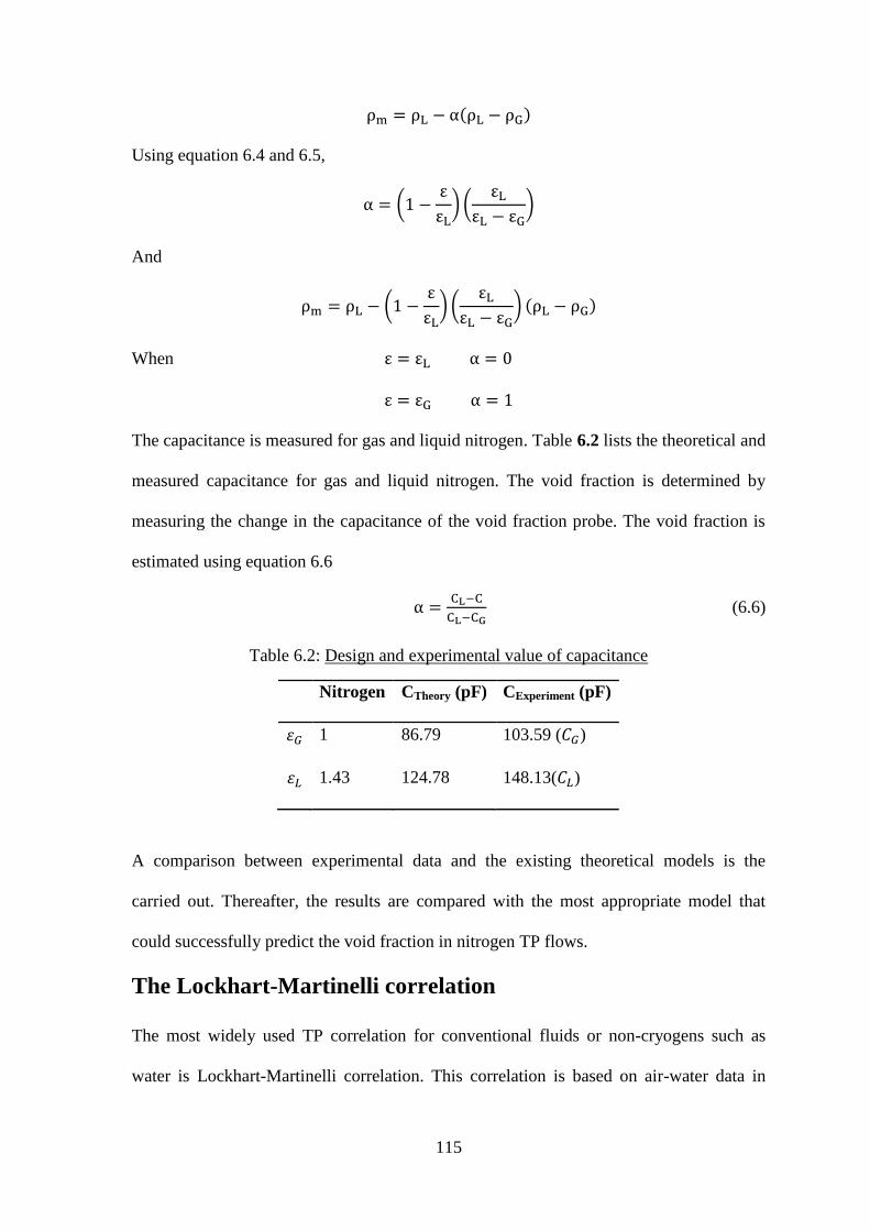
115

ρm = ρL − α(ρL − ρG)

Using equation 6.4 and 6.5,

α = (1 −ε

εL) (

εL

εL − εG)

And

ρm = ρL − (1 −ε

εL) (

εL

εL − εG) (ρL − ρG)

When ε = εL α = 0

ε = εG α = 1

The capacitance is measured for gas and liquid nitrogen. Table 6.2 lists the theoretical and

measured capacitance for gas and liquid nitrogen. The void fraction is determined by

measuring the change in the capacitance of the void fraction probe. The void fraction is

estimated using equation 6.6

α =CL−C

CL−CG (6.6)

Table 6.2: Design and experimental value of capacitance

Nitrogen CTheory (pF) CExperiment (pF)

𝜀𝐺 1 86.79 103.59 (𝐶𝐺)

𝜀𝐿 1.43 124.78 148.13(𝐶𝐿)

A comparison between experimental data and the existing theoretical models is the

carried out. Thereafter, the results are compared with the most appropriate model that

could successfully predict the void fraction in nitrogen TP flows.

The Lockhart-Martinelli correlation

The most widely used TP correlation for conventional fluids or non-cryogens such as

water is Lockhart-Martinelli correlation. This correlation is based on air-water data in

116

horizontal tubes as discussed in chapter 1. The LM void fraction correlation is expressed

as given in Table 1.2.

Figure 6.9-Figure 6.12, shows the comparisons between void fraction data of nitrogen at

various vapor quality obtained at the constant gas mass flow and the LM void fraction

correlation. The comparison shows large differences between the predicted and the

measured void fraction.

This may be due to the fact that this correlation is originally derived from air-water data

in horizontal tube whereas the present study is for cryogen (nitrogen) in a horizontal

orientation.

The homogeneous flow model

In the homogeneous flow model, the basic assumptions are that the TP are moving with at

the same velocity without considering detail description of flow pattern. The slip ratio is

always equal to unity. Thus, there is no effect of mass velocity that is considered in this

model. The void fraction by the homogeneous model is expressed as given in Table 1.2.

The comparison between the prediction by homogenous model and experimentally

measured void fraction is shown in Figure 6.9-Figure 6.12. The measured experimental

data shows reasonable agreement with the homogeneous model. When the quality is

rather low, the deviation from the homogeneous model increases.

This discrepancy is due to the fact that, at low qualities, the slip is high and no more

negligible as per the assumption of the model. With the increase in the mass flow, the slip

decreases and approaches unity. Evidently, the comparison shows that maximum

deviation is 10% from prediction at lower quality. At higher quality, the deviation is less

than 5%.

117

Figure 6.9:Void fraction as a function of vapor quality for ṁg=0.45 g/s

Figure 6.10:Void fraction as a function of vapor quality for ṁg=0.64 g/s

118

Figure 6.11: Void fraction as a function of vapor quality for ṁg=0.78 g/s

Figure 6.12: Void fraction as a function of vapor quality for ṁg=1 g/s

119

Figure 6.13: Void fraction data as a function of vapor quality for fixed GN2 flow rate and

its comparison with the predictions of Lockhart-Martinelli, and the homogeneous model.

Further, as the gas flow is increased a better agreement is obtained because the slip ratio

approaches unity. In summary, therefore, it is concluded that the measured void fractions

fall somewhere in between the prediction of the homogeneous model and Lockhart-

Martinelli model as shown in Figure 6.13but more closer to the homogeneous model.


This study is aimed at (a) developing an appropriate sensor for void fraction

measurements (b) validation of the void fraction measurement with the developed sensor

in horizontal nitrogen TP flows. An appropriate experimental facility has been designed,

customized and developed for these purposes. The void fraction is measured by a custom

developed coaxial capacitance probe at the end of test section process line. The probe is

connected by an electronic measurement system designed and developed to measure

small changes in dielectric constant resulting from the relative densities of the flowing TP

mixtures. The experimental data of void fraction has been obtained at various constant

gas flow rates with the increasing liquid nitrogen flow rate. The experimental data

120

obtained are then compared with the prediction of the homogeneous model and Lockhart-

Martinelli model of TP flow.

This experimental investigation demonstrates that the capacitance probe technique with

indigenously developed electronic measurement system is quite accurate and novel

technique towards measuring void fraction in nitrogen TP flows. The measurement

system accurately measures void fraction in TP nitrogen with an error less than 2% for

the vapor quality 0.1 to 1. The predictions of homogeneous model agree with the void

fraction data within 10 % deviation for lower vapor quality and within 5 % for higher

vapor quality as the slip approaches the unity. On the other hand, the deviation is greater

than 15 % between the measured void and predicted void by Lockhart-Martinelli

correlation.

121

CHAPTER-VII

7. Summary and future work


7.2 Future work

122


The study of cryogenic TP flow is always complex due to lack of accurate measurement

of process parameters such as quality or mass flow rate etc. It is, therefore, better, to

begin with, the simple system and with a common cryogenic fluid to comprehend the

physical and experimental issues associated with the cryogenic TP flow. As part of the

experimental skill development, towards gaining basic understanding and hands-on

experience; a simple and smooth cryo line was first indigenously designed and fabricated.

The TP characteristics of the commonly available liquid Nitrogen were investigated in

this cryoline. The basic essential parameters such as flow rates of single-phase coolant,

the pressure drop of the single phase coolant and TP coolant, the vapor fractions in TP

flows, the voids in TP flow etc. were investigated both experimentally and theoretically.

Appropriate correlations and laws associated with single-phase flow as well as TP flow

were invoked and compared with the theoretical predictions within experimental

accuracies. Essential measurement techniques, sensors, and diagnostics needed for

characterizing the fluid flows, associated data acquisitions etc. have been learned in these

initial experimentations and exercises. This study further gave better hands-on experience

to deal with a more complex cryogenic TP flow such as with liquid helium in

superconducting magnets, which was the ultimate aim of this doctoral work. Studying of

TP characteristics in the state-of-the-art CICC configurations which are relevant for

several laboratory applications as well as for fusion-relevant magnet systems are even

more challenging and interesting. In such configurations, the simulation of thermal-

hydraulics related studies is quite difficult, since there is the absence of streamlines or

defined boundary layers. Further, the friction factor correlation has enough inaccuracies

and, the correlations are valid only within the specific range of Reynolds Number. All

these aspects actually make these studies more interesting and challenging i.e. to predict

123

the behavior of cryogenic TP flow in a CICC like hydraulic channel or in a

superconducting magnet. These initial experimental efforts and the results have been

elaborately discussed in chapter-2 of the thesis.

Since the 1980s, with the advent of CICC configurations, it has been rapidly as the

candidate conductor for fusion-relevant magnet systems by the Fusion community.

Further, cooling of the CICC wound large-scale superconducting magnets using single

phase of helium has been largely preferred. The foreseen advantages have been the

extrapolation of well-established analytical formulations of the single-phase flow and

associated thermo-hydraulics. It has been apprehended that TP cooling of CICC

configured magnet systems could suffer from flow chocking and other associated

instabilities and hence are disadvantageous. The occurrences of flow chocking or flow

instabilities in TP cooled magnets are thermo-hydraulically sensitive to certain process

parameters. TP flows have very well defined flow patterns and flow regimes. Since the

TP flow exploits the latent heat instead of enthalpy, it offers significant advantages

towards cryo-stability. Introduction of cryogenic TP flow provides enhanced heat transfer.

Resultantly, the same magnets can be TP cooled with significantly lowered the mass

flow rate, which could be~ 5 to 6 time as compared to the single phase flow cooling for

same cryogenic stability. In practice, these measures can save the precious cold power of

the cryogenic machine. Thus TP cooling is significantly cost-effective in practice. One

such example of TP cooled superconducting magnets operating successfully in plasma

operation is of the Toroidal Field Magnet system of the First Indian Steady State

Superconducting Tokamak (SST-1). Previously, magnets of the Soviet-made tokamak T-

7 [83] and T-15 [84], has been operated successfully being TP cooled. However, these

conductors were largely monolithic with a defined helium flow passage. The POLO [85]

conductors which were early versions of CICC with a defined flow passage in the 1980s

124

also have been cooled with TP and operated successfully. In the context of Tokamak,

SST-1 TF magnets are the first medium sized magnets being operated with TP

successfully in Tokamak plasma applications. Chapter-3 of the thesis has analyzed the TP

characteristics of the SST-1 TF magnets from three experimental campaigns. In these

detailed studies, the pressure head and quality factor analysis have been carried out for

the SST-1 TF magnets. Using Lockhart Martinelli relations and actual experimental data

of the SST-1 TF magnets, the vapor quality has been estimated. The results demonstrate

that as the mass flow rate increases, corresponding pressure drop increases and hence the

vapor quality decreases for a given heat load. These analyses have proved to be one of the

efficient tools for analyzing the TP flow characteristics in complex flow geometry like

CICC.

Performances of the TP cooled medium size Tokamak superconducting magnets being

shown to be excellent; the next investigation was to ascertain its functional

appropriateness on a fusion relevant prototype conductor of CICC configurations. For

these purpose, the investigations of the envisaged characteristics of a TP cooled prototype

CICC had been undertaken in Chapter-4 of the thesis work. The pressure drop and

quality factor analysis have been carried for this prototype CICC wound high field

superconducting magnet for a number of realistic heat flux and inlet mass flow rates. The

`effective temperatures’ have also been predicted. These analyses would be useful for

future TP flow related experiments in a complex geometry like CICC. The results

obtained also state that as the mass flow rate increases, corresponding pressure drop

increases and hence the vapor quality decreases for a given heat flux. Analyses have

shown results that CICC wound fusion magnets may be operated in the TP flow of helium

under certain operational envelopes. The TP cooling of CICC do get into risks of flow

choking and thermo-acrostic instabilities possibilities, but ensuring single phase sub-

125

cooling at the inlet these possibilities in practice could be reduced significantly or even

eliminated for certain heat flux and operating parameters. Even though the TP cooling

and its thermo-hydraulics are complex in nature to realize, by using the prescriptions

discussed above, reasonable predictions of these essential quantities of the flow scheme

are feasible (effective temperature, pressure drop and vapor quality). These information

may be helpful in practical operations of TP cooled magnets in future.

Next, a dedicated experiment has been designed to study the different flow pattern that

can exist in case of the cryogenic TP flow of liquid nitrogen in chapter-5 of the thesis. An

indigenous test facility has been designed and developed for this purpose. This work is a

maiden attempt in compiling a database through experiments of the flow structures, the

mass flow rates, the vapor quality and predicted void fraction in various flow regimes

involving TP nitrogen flow in a horizontal configuration. LN2 and gaseous nitrogen (GN2)

are forced to flow separately through a test section as a part of calibration of the

experimental system. Thereafter, by varying liquid Nitrogen flow rates with the constant

gas flow, the variation of a void fraction as a function of a quality factor has been

investigated. Void fraction has been successfully predicted for a range of experimental

quality factor using Lockhart-Martinelli, Fauske, Lenvi and Homogeneous TP flow

models. Using standard flow regime models; Backer’s regime map, The Taitel, The

Dukler and Wojtan flow regime map have been analyzed. These have been compared

with the flow visualization using fast Digital camera. Different flow patterns have been

realized using different process parameters leading to a comprehensive investigation of

TP nitrogen flow in a horizontal configuration. This work provides a critical database that

will be helpful towards the development and improvement of models and correlations

involving cryogenic TP cooling. The experimental database could also be used in the

development of an appropriate void sensor or quality meter. In fact, the developments of

126

the void sensor, its performance in cryogenic TP flow scenarios have been elaborated in

the next chapter-6 of the thesis.

It has been very challenging and interesting to develop the TP flow void sensor for

cryogenic services. In this work, the commonly available and used LN2 has been taken as

the working cryogenic fluid for which void sensor has been developed. This void sensor

developed is subsequently tested and validated in an indigenous test facility. The

electronic circuit for the void sensor has also been developed indigenously to facilitate a

precise measurement of the cryogenic TP nitrogen void fraction. The measuring principle

is based on measuring the capacitances of the fluid. Experimental values of a void

fraction are obtained by measuring the changes in the capacitance of coaxial capacitive

sensor due to TP flow. Here, the appreciable difference of the dielectric properties of

nitrogen fluid in vapor and liquid phase is exploited. The study was carried for the void

fraction measurement in horizontal nitrogen TP flows. An experimental apparatus was

custom designed and developed for this purpose. The void fraction was measured by a

coaxial capacitance probe at the end of test section process line. The probe was connected

by an electronic measurement system designed and developed to measure small changes

in dielectric constant results due to change in the density of the TP mixture. The

experiment data of void fraction was obtained at various constant gas flow rate and

increasing liquid nitrogen flow rate. The experimental data were then compared with the

prediction of the homogeneous model and Lockhart-Martinelli model of TP flow.

The study showed that the capacitance probe technique with developed electronic

measurement system is a very novel technique to measure void fraction in nitrogen TP

flows. The measurement system accurately measures void fraction in TP nitrogen with an

error less than 2% for the vapor quality 0.1 to 1. The predictions of homogeneous model

agree with the void fraction data within 10 % deviation for lower vapor quality and within

127

5 % for higher vapor quality as the slip approaches the unity. The large deviation is

noticed between the measured void and predicted void by Lockhart-Martinelli correlation.

7.2 Future work

During the present thesis work, the study was mainly focused up to liquid nitrogen based

characterization and flow pattern study in case of TP flow. In order to carry out such

study, the indigenous cryo line along with the customized lab experimental test set-up

was developed. During the study, a void fraction measurement system for horizontal flow

configuration was realized. It was also interesting to study the different flow patterns

while tuning the process parameters in case of liquid nitrogen TP flow. It is evident that

flow pattern, flow regime and technical information on quality or void fraction are

extremely critical information to exploit the TP flow involving cryogens. It will be useful

in future to study and invent an accurate and novel sensor in terms of a void fraction or

quality factor measurement for TP liquid helium or liquid hydrogen applications. Liquid

helium and liquid hydrogen have several laboratory, fusion and space applications. Such

database would be quite beneficial for these spectrums of applications.

Flow pattern studies revealed that depending upon proper tuning of given process

parameters; one can change the flow pattern. Some of the flow patterns are undesirable in

terms of the industrial process where the pump performance can be degraded and impeller

can be completely damaged. Such flow patterns in TP flow must be quantified. Using the

database of flow pattern, one can avoid such process parameters and regimes. Especially,

similar studies can be done in case of liquid hydrogen TP flow where one can save the

cryogenic engine and some of the parts of the Rocket Propulsion system. Similarly, in

fusion relevant magnets cooled with TP liquid helium or Magnetic Resonance Imaging

applications, in Nuclear Magnetic Resonance or in High Gradient Magnetic Separators

128

applications; such regimes could be avoided while benefiting from the large Cryo-

stabilities from TP flow.

129

Bibliography

[1] Randall Barron, “Cryogenic systems”, 1985, ISBN 13: 9780195035674.

[2] Van Sciver, Steven W., “Helium Cryogenics”, 2012, ISBN 978-1-4419-9979-5.

[3] Filina, N. N., and Weisend, J. G., “Cryogenic Two-Phase Flow: Applications to

Large-Scale Systems”, 1996, Cambridge University Press, New York, USA.

[4] Bronson, J. C., Edeskuty, J. F., Fretwell, J. H., Hammel, E. F., Keller, W. E.,

Meier, K. L., Schuch, A. F., and Willis, W. L., 1962, “Problems in Cool-down of

Cryogenic Systems,” Advances in Cryogenic Engineering, Vol. 7, pp. 198-205.

[5] John G. Collier and John R. Thome., “Convective Boiling and Condensation,

Third Edition”, 1996, ISBN-13: 978-0198562962.

[6] Butterworth, D., “A comparison of some void-fraction relationships for co-current

gas-liquid flow”, Int. J. Multiphase Flow 1, 845–850, 1975.

[7] Melkamu A. et al., “Comparison of void fraction correlations for different flow

patterns in horizontal and upward inclined pipes”, International Journal of

Multiphase Flow 33 (2007) 347–370.

[8] Lockhart, R.W., Martinelli, R.C., “Proposed correlation of data for isothermal

two-phase, two component flows in pipes”, Chem. Eng. Progr. 45, 39–48, 1949.

[9] Fauske, H., “Critical two-phase, steam–water flows”, In: Proceedings of the 1961

Heat Transfer and Fluid Mechanics Institute. Stanford University Press, Stanford,

CA, pp. 79–89, 1961.

[10] Levy, S. “Steam slip theoretical prediction from momentum model”, Trans.

ASME, J. Heat Transfer 82, 113–119, 1960.

[11] Levy, S., "Prediction of Two-Phase Critical Flow Rate”, J. Heat Trans., Series C,

87, 53, 1965.

130

[12] Jelliffe Kevin Jackson, “Cryogenic two-phase flow during chill down flow

transition and nucleate boiling heat transfer,” Ph.d. Thesis, University of Florida,

2006.

[13] A.I. Alexeyev et al. , “Flow patterns of two-phase helium in horizontal

channels’’, Cryogenics 1991 Vol 31 May pp. 330-337

[14] Benard Rousset et al., “Two-phase visualization at cryogenic temperature’’,

Cryogenics 41 (2001) 443–451

[15] Benard Rousset et al., “Visualization in the cryogenic environment: Application

to two-phase studies” Cryogenics 49 (2009) 554–564’

[16] S. Pradhan et al., “The first experiment in SST-1,” Nucl. Fusion, vol. 55, 2015,

Art. no. 104009.

[17] S. Pradhan et al., “First operational results with the SST-1 superconducting

magnet & its cryogenics,” in Proc. 25th Int. Cryogenic Eng. Conf. Int. Cryogenic

Mater. Conf., vol. 67, 2015, pp. 756–761.

[18] T. Haruyama et al., “Pressure drop of two-phase helium flowing in a large

solenoidal magnet cooling path and a long transfer line,” Cryogenics, vol. 36, pp.

465–469, 1996.

[19] T. Haruyama, T. Mito, Y. Doi, and A. Yamamoto, “Pressure drop in forced two-

phase cooling of the large thin superconducting solenoid,” Adv. Cryogenic Eng.,

vol. 33, pp. 543–549, 1988.

[20] Haruyama, T., “Cryogenic characteristics of a large thin superconducting

solenoidal magnet cooled by forced two-phase helium”, paper presented at

ICECl5, Genoa, Italy (7-10 June 1994).

131

[21] Burke, J. C., Byrnes, R. W., Post, A. H., and Ruccia, F. E., 1960, “Pressurized

Cooldown of Cryogenic Transfer Lines,” Advances in Cryogenic Engineering,

Vol. 4, pp. 378-394.

[22] Prasad, K. A. D., Srinivasan, K., and Murthy, M. V. K., 1974, “Cool-down of

Foam Insulated Cryogenic Transfer Lines,” Cryogenics, Vol. 14, No.11, pp. 615-

617.

[23] J. M. Jurns, “Description of liquid nitrogen experimental test facility”,

Cryogenics 1992 Vol 32, No 2, 173-178, 1991.

[24] R. Panchal et al., “Design and engineering validation of venturi flow meter for

current feeder system of SST 1,” Indian Journal of cryogenics, vol. 39, 2014 pp.

53-57.

[25] Dipak Patel, “Thermal anchoring of wires in large scale superconducting coil test

experiment”, Fusion Engineering and Design 88 (2013) 374–379.

[26] F. Hosono, U.D.C. HITACHI CABLE REVIEW No.20 (August 2001) 101-104.

[27] S. Kedia and S. Pradhan, “Effect of temperature on hydraulic parameters of

cable-in-conduit-conductor of SST-1,” J. Supercond. Novel Magn., vol. 26, pp.

1289–1296, 2013.

[28] S. Pradhan, “Cable-in-Conduit Conductor for Superconducting Magnets of SST-

1 Tokamak”, 3rd IAEA TCM on Steady State Operation of Magnetic Fusion

Devices, March 2002.

[29] A.N. Sharma, U. Prasad, K. Doshi, P. Varmora, Y. Khristi, D. Patel, et al.,

“Cryogenic acceptance tests of SST-1 superconducting coils”, IEEE Trans. Appl.

Supercond. 25 (2) (2015) 420010.

[30] S.Pradhan, et al., “First Engineering Validation Results of SST-1 TF Magnets

System”, IEEE Trans. Appl. Supercond., 24(3), (2014) 4202206.

132

[31] Rohit Panchal et al., “Operational experience with the supercritical helium during

the TF coils tests campaign of SST-1”, AIP Conference Proceedings 1434, 1407

(2012).

[32] G K Singh et al. ,“Prediction of helium vapor quality in steady state Two-phase

operation of SST-1 Superconducting Toroidal field magnets”, IEEE Transactions

on Applied Superconductivity, March 2018, Vol. 28, Issue: 2.

[33] S.P. Gorbachev, “Calculating the hydraulic characteristics of Two-Phase

HELIUM Circulation Systems”, Vol.41, pp. 396-401 (1980).

[34] H. M. Mekisso, “Comparison of frictional pressure drop correlations for

isothermal two-phase horizontal flow,” M.S. thesis, Graduate college of the

Oklahoma State University, USA, 2013.

[35] V. L. Tanna, “Design and Analysis of the Superconducting Current Feeder

System for the International Thermonuclear Experimental Reactor (ITER)”, PhD

thesis, Institut für Technische Physik, Forschungszentrum Karlsruhe GmbH,

Karlsruhe, Germany 2006.

[36] G K Singh et al., “Two-Phase Helium Cooling Characteristics in Cable-in-

Conduit Conductors”, Indian Journal of Cryogenics, 2018, Vol. 43, Issue: 1,137-

142.

[37] T. Rane, A. Chakravarty, R. K. Singh, and T. Singh, “Improved correlations for

computations of liquid helium two phase flow in cryogenic transfer lines,”

Cryogenics, vol. 51, pp. 27–33, 2011.

[38] P. Zhang et al, “Two-phase flow characteristics of liquid nitrogen in vertically

upward 0.5 and 1.0 mm micro-tubes: Visualization studies”, Cryogenics, Vol. 49,

pp. 565-575 (2009).

133

[39] X.Fu, S.L. Qi, Zhang, R.Z. Wang, “Visualization of flow boiling of liquid

nitrogen in a vertical mini channel”, International journal of multiphase flow 34,

2008, 333-351.

[40] Christopher James Velat, “Experiments in cryogenic two phase flow”, M.S

Thesis, University of Florida, USA, 2004.

[41] S. Kakac a, B. Bon, “A Review of two-phase flow dynamic instabilities in tube

boiling systems”, International Journal of Heat and Mass Transfer 51 (2008) 399–

433.

[42] M. M. Padkiet. et al, “Bifurcation analysis of pressure-drop oscillations and the

Ledinegg instability”, J. Heat Mass 7’nmfer. Vol. 35, No. 2, pp. S25-532, 1992

[43] Y. Ding and S. Kaka, “Dynamic Instabilities of Boiling Two-Phase Flow in a

Single Horizontal Channel”, Experimental Thermal and Fluid Science 1995;

11:327-342.

[44] J.M. Jurns et al.,’’Liquid nitrogen experimental test facility’’, Cryogenics Vol 32,

No 2 pp. 173-178, 1992.

[45] Chen Jianye et al., “Experimental results of flooding experiments in an inclined

tube with liquid nitrogen and its vapor’’, Cryogenics 62 (2014) 1–6.

[46] A.I. Alexeyev et al., “Flow patterns of two-phase helium in horizontal channels’’,

Cryogenics 1991 Vol 31 May pp. 330-337.

[47] Benard Rousset et al., “Two-phase visualization at cryogenic temperature’’

Cryogenics 41 (2001) 443–451.

[48] Benard Rousset et al.,”Visualization in the cryogenic environment: Application

to two-phase studies” Cryogenics 49 (2009) 554–564.

134

[49] J. N. Chung, “Cryogenic Two-Phase Flow and Boiling Heat Transfer During

Pipe Chilldown”, 37th AIAA Thermo physics Conference, 28 June - 1 July 2004,

Portland, Oregon.

[50] G K Singh et al., “Experimental studies of two-phase flow characteristics and

void fraction prediction in horizontal two-phase nitrogen flow”, Cryogenics, June

2019, Vol. 100, Pages 77-84.

[51] Baker, O., “Simultaneous Flow of Oil and Gas,” Oil and Gas Journal, Vol. 53, pp.

185-195, 1954.

[52] Taitel, Y., and Dukler, A. E., “A Model for Predicting Flow Regime Transitions

in Horizontal and Near Horizontal Gas-Liquid Flow,” AIChE Journal, Vol. 22, No.

1, pp. 47-55, 1976.

[53] Wojtan, L., Ursenbacher, T., and Thome, J. R., “Investigation of Flow Boiling in

Horizontal Tubes: Part I – A New Diabatic Two-Phase Flow Pattern Map,”

International Journal of Heat and Mass Transfer, Vol 48, pp. 2955-2969, 2005.

[54] Kattan, N., Thome, J. R., and Favrat, D., “Flow Boiling in Horizontal Tubes: Part

1-Development of a Diabatic Two-Phase Flow Pattern Map,” Journal of Heat

Transfer, Vol. 120, pp. 140-147, 1998.

[55] Steiner, D., VDI-Wärmeatlas (VDI Heat Atlas), Verein Deutscher Ingenieure, ed.,

VDI-Gessellschaft Verfahren stechnik und Chemieingengenieurwesen (GCV),

Düsseldorf, Germany, 1993.

[56] G K Singh et al., “Development of a Precise electronic system for cryogenic two-

phase flow void fraction measurement”, Journal of Electrical and Electronics

Engineering, Oct. 2018, Vol. 11, nr. 2, 27-30.

[57] Ceccio SL, George DL. “A review of electrical impedance techniques for the

measurement of multiphase flows”, J Fluid Eng 1996; 118:391–9.

135

[58] Juliá JE, Harteveld WK, Mudde RF, Van den Akker HE. “On the accuracy of the

void fraction measurements using optical probes in bubbly flows”, Rev Sci

Instrum 2005; 76:035103.

[59] Ahmed WH. “Capacitance sensors for void-fraction measurements and flow

pattern identification in the air–oil two-phase flow. Sensors” J, IEEE 2006;6

(5):1153–63.

[60] Srisomba R, Mahian O, Dalkilic AS, Wongwises S., “Measurement of the void

fraction of R-134a flowing through a horizontal tube”, Int Commun Heat Mass

2014;56:8–14.

[61] Uesawa S, Kaneko A, Abe Y., “Measurement of void fraction in dispersed

bubbly flow containing micro-bubbles with the constant electric current method”,

Flow Meas Instrum 2012;24:50–62.

[62] Tan C, Dong F, Wu M., “Identification of gas/liquid two-phase flow regime

through ERT-based measurement and feature extraction”, Flow Meas Instrum

2007; 18(5):255–61.

[63] Kerpel KD, Keulenaer TD, Schampheleire SD, Paepe MD., “Capacitance sensor

measurements of upward and downward two-phase flow in vertical return bends”,

Int J Multiphase Flow 2014;64:1–10.

[64] Canière H, Bauwens B, Joen CT, De Paepe M., “Mapping of horizontal

refrigerant two-phase flow patterns based on clustering of capacitive sensor

signals”, Int J Heat Mass Tran 2010;53:5298–307.

[65] A.K. Khalil., “Cryogenic two-phase flow characteristics of helium I in vertical

tubes”, University of Wisconsin-Madison, 1978.

136

[66] Ousaka A, Kariyasaki A, Lucas D, Vierow K, Vallee C, Hogan K.,“The effects

of surface tension on flooding in counter-current two-phase flow in an inclined

tube”, ExpTherm Fluid Sci 2010;34:813–26.

[67] Carapelle A, Collette J., “Gamma-ray attenuation for measuring cryogenic slush

mixture density”, Nucl Instrum Methods Phys Res Sect B: Beam Interact Mater

Atoms 2005; 229:111–6.

[68] Bartlit, J.R., and Lester, D.H., Report LA-DC-9706, Los Alamos Scientific

Laboratory, New Mexico,1966

[69] Ohira K. “Development of density and mass flow rate measurement technologies

for slush hydrogen”, Cryogenics 2004; 44:59–68.

[70] Filippov YP, Kakorin ID, Kovrizhnykh AM. “New solutions to produce a

cryogenic void fraction sensor of round cross-section and its applications”,

Cryogenics 2013; 57:55–62.

[71] Filippov YP. “How to measure void fraction of two-phase cryogenic flows”,

Cryogenics 2001; 41(5–6):327–34.

[72] Filippov YP, Kovrizhnykh AM, Romanov SV., “Improvement of rf-system to

measure void fraction of cryogens”, Advances in cryogenic engineering. US:

Springer; 2000. pp. 1911–8.

[73] Jiang YY, Zhang P.,“Density determination of slush nitrogen by the improved

capacitance-type densimeter”, Exp Therm Fluid Sci 2011;35:328–37.

[74] Kerpel KD, Ameel B, T’Joen C, Canière H, Paepe MD. ,“Flow regime based

calibration of a capacitive void fraction sensor for small diameter tubes”, Int J

Refrig 2013;36:390–401.

[75] Das R, Pattanayak S. “Flow regime identification in cryogenic gas-liquid flow

through vertical tubes”, Cryogenics 1995; 35:393–8.

137

[76] S. M. Huang, A. L. Stott, R. G. Green and M. S. Beck, “Electronics Transducers

for Industrial measurement of low value capacitances,” Journal of Physics E:

Sci&Instrum., vol.21, pp. 242-250, 1988.

[77] C. Corney, “A universal four pair impedance bridge,” IEEE Tran.

Instrumentation and Measurement, vol. IM-28, pp. 211-215, 1979.

[78] K. Kobayashi, S.Okamoto, and M. Sukigara, “A Capacitance relaxation method

of studying surface states at the semiconductor-liquid junction,” J. Electroanal.

Chem., vol. 225, pp. 79-92, 1987.

[79] M.Yamada, T Takebayashi, S. Notoyama, and K. Watanabe, “A switched

capacitor interface for capacitive transducer,” IEEE Tran. Instrumentation and

Measurement, Vol. 41, no. 1 pp. 81-86, February 1992.

[80] J. K-Rasmussen and W. Q. Wang, “A compact electrical capacitance tomography

system” Proc. IEEE International Workshop on Imaging Systems and Techniques

(IST 2008), Chania Greece, September 10-12, 2008.

[81] CD4093BM CD4093BC Quad 2-Input NAND Schmitt Trigger. Texas

Instruments, Literature Number: SNOS369A.

[82] Gautam Sarkar, Anjan Rakshit, Amitava Chatarjee, Kesab Bhattacharya, “Low

Value Capacitance Measurement System with Adjustable Lead Capacitance

Compensation,” World Academy of Science Engineering and Technology Vol.7

No.1 2013.

[83] D. P. Ivanov, V. E. Keilin, 13. A. Stavissky, N. A. Chernoplekov, “Some results

from the t-7 tokamak superconducting magnet test program”, IEEE Transactions

on Magnetics, vol. 15, no. 1, January 1979.

[84] N.A. Chernoplekov, “The system and test results for the Tokamak T-15 magnet”,

Fusion Engineering and Design 20 (1993) 55-63.

138

[85] Alexander W Chao, Weiren Chou – Science, “Reviews of Accelerator Science

and Technology: Volume 5: Applications of superconducting technologies to

accelerators”, ISBN 978-981-444994-6, PP. 108.

STUDY OF TWO-PHASE FLOWS IN FUSION MAGNETS

Documents

Transcript of STUDY OF TWO-PHASE FLOWS IN FUSION MAGNETS