Treball final de grau

GRAU D’ENGINYERIA INFORMÀTICA

Facultat de Matemàtiques i InformàticaUniversitat de Barcelona

STUDY OF RECONSTRUCTIONICA FOR FEATURE

EXTRACTION IN IMAGES ANDSIGNALS

Autor: Marc Beltrán Segarra

Director: Laura Igual MuñozRealitzat a: Departament de Matemàtiques i Informàtica

Barcelona, June 22, 2017

AbstractDuring the last years, neural networks have become a vehicular discipline in thefield of machine learning. At the same time, classical machine learning methodshave become easier to use due to the availability of higher computational power.The goal of this project is to reconstruct a classical machine learning algorithm usedfor feature and source extraction (ICA) using neural networks. This reconstructioncould bypass some of the drawbacks presents when using ICA. We have studied howthe reconstruction operates under different conditions and performed a comparisonwith the classical algorithm that we reconstructed.

ResumLes xarxes neuronals s’han convertit en una disciplina fonamental a dins del campde l’aprenentatge autònom o machine learning. Al mateix temps, mètodes clàwsicsd’aquest camp han passat a ser més fàcils d’utilitzar a causa dels avanços tecnològics.L’objectiu d’aquest projecte és la reconstrucció d’un d’aquests algoritmes clàssicsper l’extracció de característiques i fonts (ICA) utilitzant xarxes neuronals. Aquestareconstrucció podria evitar alguns dels inconvenients que existeixen alhora d’utilitzarICA. Hem estudiat com la reconstrucció opera sota diferents condicions i realitzatuna comparació amb l’algorisme clàssic que hem reconstruït.

ResumenLas redes neuronales se han convertido en una disciplina fundamental dentro delcampo del aprendizaje automático o machine learning. Al mismo tiempo, métodosclásicos de este campo han pasado a ser más fáciles de utilizar debido a los avancestecnológicos. El objetivo de este proyecto es la reconstrucción de uno de estosalgoritmos clásicos (ICA) usando redes neuronales. Esta reconstrucción podá evitaralgunos de los inconvenientes que existen cuando se usa ICA. Hemos estudiado comola reconstrucción funciona bajo distintas condiciones y realizado una comparacióncon el algoritmo clásico que hemos reconstruido.

1

Contents1 Introduction 4

1.1 Context . . . . . . . . . . . . . . . . . . . . . . . . . . . . . . . . . . 41.2 Objectives . . . . . . . . . . . . . . . . . . . . . . . . . . . . . . . . . 41.3 Motivation . . . . . . . . . . . . . . . . . . . . . . . . . . . . . . . . . 41.4 Structure of the document . . . . . . . . . . . . . . . . . . . . . . . . 4

2 Neural Networks 62.1 Neuron . . . . . . . . . . . . . . . . . . . . . . . . . . . . . . . . . . . 62.2 Neural Network model . . . . . . . . . . . . . . . . . . . . . . . . . . 6

2.2.1 Forward propagation . . . . . . . . . . . . . . . . . . . . . . . 72.3 Activation functions . . . . . . . . . . . . . . . . . . . . . . . . . . . 82.4 Main types of neural networks . . . . . . . . . . . . . . . . . . . . . . 9

2.4.1 Supervised neural networks . . . . . . . . . . . . . . . . . . . 92.4.2 Unsupervised neural networks . . . . . . . . . . . . . . . . . . 9

2.5 Learning in a neural network . . . . . . . . . . . . . . . . . . . . . . . 10

3 Autoencoders 113.1 Introduction . . . . . . . . . . . . . . . . . . . . . . . . . . . . . . . . 113.2 Definition . . . . . . . . . . . . . . . . . . . . . . . . . . . . . . . . . 113.3 Interpretation . . . . . . . . . . . . . . . . . . . . . . . . . . . . . . . 12

4 Sparsity and Sparse Coding 144.1 Sparsity Norms . . . . . . . . . . . . . . . . . . . . . . . . . . . . . . 15

5 Principal Component Analysis 165.1 Introduction . . . . . . . . . . . . . . . . . . . . . . . . . . . . . . . . 165.2 Definition . . . . . . . . . . . . . . . . . . . . . . . . . . . . . . . . . 165.3 Applications . . . . . . . . . . . . . . . . . . . . . . . . . . . . . . . . 17

6 Independent Component Analysis 186.1 Introduction . . . . . . . . . . . . . . . . . . . . . . . . . . . . . . . . 186.2 Definition . . . . . . . . . . . . . . . . . . . . . . . . . . . . . . . . . 186.3 Algorithm: FastICA . . . . . . . . . . . . . . . . . . . . . . . . . . . 18

6.3.1 FastICA for single component extraction . . . . . . . . . . . . 186.3.2 FastICA for multiple component extraction . . . . . . . . . . . 19

6.4 Interpretation . . . . . . . . . . . . . . . . . . . . . . . . . . . . . . . 196.4.1 ICA on images . . . . . . . . . . . . . . . . . . . . . . . . . . 196.4.2 ICA on signals . . . . . . . . . . . . . . . . . . . . . . . . . . 20

6.5 ICA drawbacks . . . . . . . . . . . . . . . . . . . . . . . . . . . . . . 21

7 Reconstruction ICA 227.1 Introduction . . . . . . . . . . . . . . . . . . . . . . . . . . . . . . . . 227.2 Definition . . . . . . . . . . . . . . . . . . . . . . . . . . . . . . . . . 227.3 Implementation . . . . . . . . . . . . . . . . . . . . . . . . . . . . . . 227.4 Relationship with Autoencoders and Sparse Coding . . . . . . . . . . 24

2

8 Programming and libraries 268.1 MATLAB . . . . . . . . . . . . . . . . . . . . . . . . . . . . . . . . . 268.2 PCA and ICA Package . . . . . . . . . . . . . . . . . . . . . . . . . . 26

8.2.1 minFunc . . . . . . . . . . . . . . . . . . . . . . . . . . . . . . 268.2.2 SoftMax Classifier . . . . . . . . . . . . . . . . . . . . . . . . 268.2.3 UFLDL MATLAB Modules . . . . . . . . . . . . . . . . . . . 27

9 Experiments 289.1 Dataset . . . . . . . . . . . . . . . . . . . . . . . . . . . . . . . . . . 289.2 Classification test . . . . . . . . . . . . . . . . . . . . . . . . . . . . . 29

9.2.1 Softmax classifier . . . . . . . . . . . . . . . . . . . . . . . . . 299.2.2 Performance tests . . . . . . . . . . . . . . . . . . . . . . . . . 29

9.3 RICA parameter analysis . . . . . . . . . . . . . . . . . . . . . . . . . 299.3.1 Number of features . . . . . . . . . . . . . . . . . . . . . . . . 309.3.2 Number of iterations . . . . . . . . . . . . . . . . . . . . . . . 359.3.3 Value of λ . . . . . . . . . . . . . . . . . . . . . . . . . . . . . 36

9.4 Comparison of PCA, ICA and RICA . . . . . . . . . . . . . . . . . . 379.4.1 Convolution for image processing . . . . . . . . . . . . . . . . 379.4.2 Visual comparison of features extracted with ICA and RICA . 389.4.3 PCA . . . . . . . . . . . . . . . . . . . . . . . . . . . . . . . . 39

10 Conclusions 4010.1 Proposed objectives . . . . . . . . . . . . . . . . . . . . . . . . . . . . 4010.2 Future work . . . . . . . . . . . . . . . . . . . . . . . . . . . . . . . . 40

3

1 Introduction

1.1 Context

Historically, tasks such as object or speech recognition have been tough to handleby computers, despite humans being close to perfect with them. This was causedby the lack of powerful hardware which prevented researchers to work in complexprogramming models that required high computational power.

Nowadays, new types of programming have appeared thanks to technologicalprogress and the widespread availability of powerful hardware such as GPUs. Thishas allowed programmers and researchers to implement new algorithms and pro-gramming methodologies that rely on iterative methods that require a high numberof operations done by the computer. These methods can be used to work with highdimensional data, such as images or signals, and tackle problems such as classifica-tion or clustering tasks when dealing with image or sound data.

Neural networks are programming models based on emulating how the humanbrain operates by creating a network of interconnected entities that feed off eachother. Despite them being created over 20 years ago, they were not as useful as theyare now because the training process had a high computational cost.

On the other hand, classical machine learning techniques such as Principal Com-ponent Analysis or Independent Component Analysis have become more availableand easier to use too, but still have some limitations.

1.2 Objectives

The objective of this project is to study the relationship between neural networktechniques and classical machine learning methods, by studying a reconstructionof Independent Component Analysis (ICA) that is created using structures andproperties of neural networks. The study is comprised of a comparison test betweenthe reconstructed version of ICA (RICA) and the original ICA, as well as an analysison how varying different parameters in RICA affects the results.

1.3 Motivation

The motivation for this project comes from the desire to understand how bothneural networks and classical machine learning methods work, by studying a productthat comes from both branches of machine learning. Both of these areas are leftuntouched in the current study plan of the Computer Engineering Degree, so thispresents a unique opportunity to dive into a field that is and will be crucial forresearch.

The starting point of the project comes from a tutorial on Unsupervised FeatureLearning and Deep Learning from the University of Standford [1]

1.4 Structure of the document

This document is separated into three big blocks.The first one is comprised of the theoretical sections that are needed in order to

understand Reconstruction ICA, the main focus of the project. This block includes

4

sections 2 to 6. Here we will look at a brief overview of the different techniques thatlead to, or are related to, Reconstruction ICA.

The second block is formed by section 7, which dives into Reconstruction ICAand its relationships to the other parts of the project that lead up to it.

The third block is comprised of the practical side of the project. This includesthe experiments performed in order to study how Reconstruction ICA fares in apractical scenario. This is included in sections 8 and 9.

Finally, we can find the conclusions and future work in section 10.

5

2 Neural NetworksNeural networks are a computational model used in computer science and machinelearning, which is inspired in biology. It’s based on a large collection of connectedsimple units, resembling the axons in the biological brain. The objective is to beable to learn from raw data, by collaboration between the neurons to create outputstimuli that can be interpreted and used in different ways. These models can beused to approach complex problems such as image classification or voice recognitions,problems that traditional algorithms and computational techniques are not able tohandle [2].

2.1 Neuron

A neural network is composed by basic units called neurons. Neurons are intercon-nected and receive inputs from other units, to produce outputs that are then usedas input by another part of the network.

The simplest possible neural network is one comprised of a single neuron. It canbe represented as shown in figure 1.

Figure 1: Single neuron.

In this case, we have a neuron that receives 3 input terms x1, x2, and x3 (inter-cept), and outputs hw,b(x) = f(W Tx) = f(

∑3i=1Wixi + b), where:

• f is the activation function. It can be defined by several ways depending onthe application of the network, we will look into some of them later.

• W and b are the parameters of the network. W is also referred to as the weightmatrix, and will change during the training process of the network, as it learnsto "solve" the given problem.

2.2 Neural Network model

A full neural network is created by connecting together several simple neurons, insuch a way that the output of one of them is used as the input of one (or more)neurons. This creates a structure like the one shown below, where we use circlesto represent neurons and arrows to show where each output is used as input. Werepresent the input to the network as circles too which, in this example, correspondto the first layer L1 and are considered the input layer. The rightmost layer is theoutput layer. This is what is observed at the end of the process, in this case, it’s a

6

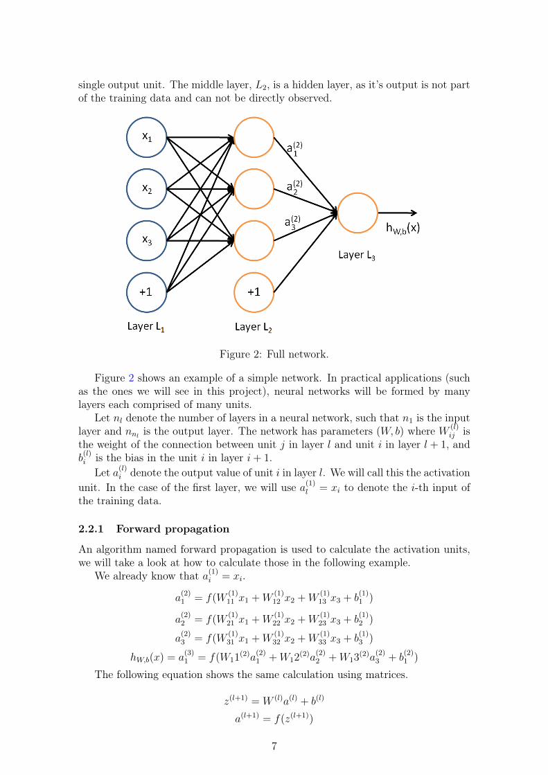
single output unit. The middle layer, L2, is a hidden layer, as it’s output is not partof the training data and can not be directly observed.

Figure 2: Full network.

Figure 2 shows an example of a simple network. In practical applications (suchas the ones we will see in this project), neural networks will be formed by manylayers each comprised of many units.

Let nl denote the number of layers in a neural network, such that n1 is the inputlayer and nnl

is the output layer. The network has parameters (W, b) where W (l)ij is

the weight of the connection between unit j in layer l and unit i in layer l + 1, andb(l)i is the bias in the unit i in layer i+ 1.

Let a(l)i denote the output value of unit i in layer l. We will call this the activationunit. In the case of the first layer, we will use a(1)l = xi to denote the i-th input ofthe training data.

2.2.1 Forward propagation

An algorithm named forward propagation is used to calculate the activation units,we will take a look at how to calculate those in the following example.

We already know that a(1)i = xi.

a(2)1 = f(W

(1)11 x1 +W

(1)12 x2 +W

(1)13 x3 + b

(1)1 )

a(2)2 = f(W

(1)21 x1 +W

(1)22 x2 +W

(1)23 x3 + b

(1)2 )

a(2)3 = f(W

(1)31 x1 +W

(1)32 x2 +W

(1)33 x3 + b

(1)3 )

hW,b(x) = a(3)1 = f(W11

(2)a(2)1 +W12

(2)a(2)2 +W13

(2)a(2)3 + b

(2)1 )

The following equation shows the same calculation using matrices.

z(l+1) = W (l)a(l) + b(l)

a(l+1) = f(z(l+1))

7

2.3 Activation functions

Activations functions (f in our examples) are applied to the inputs of the neuronsto create an output.

The most common activation functions are the following (See figure 3 for anillustration):

• Linear: The linear function is defined by

f : R→ R

f(x) = x

where k is a constant. This is the most simple activation function and isobviously C∞.

• Threshold function: The threshold (or step) function is defined by:

f : R→ {0, 1}

f(x) =

{1 iff x > 00 iff x <= 0

(1)

This function is non-differentiable in x = 0 so we can not apply gradientdescent, but it can still be used in simple neural networks.

• Rectified linear: The rectified linear function is defined by:

f : R→ [0,∞)

f(x) = max(0, x)

Similarly to the threshold function, this function isn’t non-differentiable andcan not be used with gradient descent.

• Sigmoid: The sigmoid function is defined by:

f : R→ (0, 1)

f(x) =1

1 + e−x

This function is C∞ and

f ′(x) = f(x)(1− f(x))

• Hyperbolic tangent: The hyperbolic tangent function is defined by:

f : R→ (−1, 1)

f(x) = tanh(x) =ex − e−x

ex + e−x

This function is C∞ andf ′(x) = 1− f 2(x)

8

Figure 3: Activation functions.

2.4 Main types of neural networks

There are several types of neural networks, each of which have their own structuresand characteristics. Neural networks are trained with a data input, which we calltraining set. Depending on how the task and the training set, we can differentiatetwo different types of neural networks: supervised and unsupervised networks.

2.4.1 Supervised neural networks

In supervised learning, the network is fed with a training set which includes thedesired output. This allows the network to learn by minimizing the error betweenthe predicted output and the known output. This type of learning is applied toclassification and regression problems, the first one deals with classifying data intocategories and the latter with predicting the results of a continuous function.

2.4.2 Unsupervised neural networks

Unsupervised learning deals with a training set that does not know the desiredoutput. This means that the network has to learn by using only the input data,by looking for structures in the data and working with functions created by theprogrammer.

9

2.5 Learning in a neural network

When we talk about learning in neural networks we refer to the process of modifyingthe weight values by using the backpropagation algorithm [3].

The parameters are found by optimizing functions that represent the error be-tween the outputs. These functions are called cost functions, and can be optimizedusing methods such as gradient descent [4].

The cost function represents the error between the output and the desired output.The objective is to find parameters such that this error is the closest to zero aspossible.

10

3 Autoencoders

3.1 Introduction

Autoencoders are one type of neural network that focus on compressing and de-compressing data automatically. They work by applying backpropagation lookingfor outputs that are equal to the inputs, i.e, y(i) = x(i). In figure 4 we can see thestructure of an autoencoder, where xi = x̂i.

Figure 4: Autoencoder.

3.2 Definition

An autoencoder is separated in two parts, the encoder and the decoder. The simplestcase is defined by the encoder taking an input x ∈ Rd and mapping it to z ∈ Rp

such that z = f(Wx+ b), f is an activation function, W is a weight matrix and b isa bias vector. The decoding step maps z to the reconstruction x̂ ∈ Rd, by applyingx̂ = f ′(W ′z + b′).

The objective of an autoencoder is to learn an approximation to the identityfunction, such that the output x̂i is similar to xi (hW,b(x) ≈ x). At first this mayseem a trivial problem, as simply applying the identity function, i.e. f(x) = x, wouldwork. The way we use the autoencoder is by applying constraints to the network.For instance, we could limit the number of neurons, or the number of layers. Thisway, the network will have to learn an efficient way to store the information with

11

less amount of space, so that it can be restored to be close to the input. Thiscan be seen as an application of compressing an decompressing data, with losing asfew information as possible. Taking a look at the parameters learned, we can alsodiscover interesting information about the structure of the data.

3.3 Interpretation

Lets take a look at an example of autoencoders applied to image data. Consider adataset of images representing hand-written digits, of size 28x28 pixels [5]. Examplesof 4 random digits are shown in figure 5.

Figure 5: Example of images from the dataset.

Then our input layer would have 784 units, one for each pixel. If we set up anautoencoder with one hidden layer with 200 units, we are forcing the network to learna way to compress the data such that it can be recreated as well as possible. If thedata isn’t random, the parameters learned represent how the data is structured. Infigure 6 we can see the visualization of the vectors ofW after training an autoencoderwith 200 hidden units.

In this case, and in the case of working with image data, we end up with aseries of "pen-strokes", which show the underlying structure of the original images.This can be interpreted as a series of edge detectors. Therefore, by combining theelements of this basis we can go back to the original data, which should be close tothe original image. How close it is to the original depends on many factors, suchas the correlation present in the original images or the constraint we have appliedto the network. We optimize the representation by looking for the parameters thatwill limit the error in the reconstruction fase, i.e, those that produce a x̂i closer toxi.

In this example we have looked at how limiting the number of units can help usidentify patterns in the data. But autoencoders can also be used to learn overcom-plete representations of the data as we will explore in the next section. This meanshaving a representation with a dimension higher than that of the original data.

These features learned and the new representations are helpful when facing prob-lems of recognition and classification when dealing with images, audio, and otherinput types.

12

Figure 6: W extracted from the autoencoder [6].

13

4 Sparsity and Sparse CodingTechniques such as Principal Component Analysis (PCA) allow us to represent dataefficiently by finding a basis of less dimensions in which to represent the data. Butsometimes, we wish to learn an over-complete basis in which the dimensions of theoutput will be bigger than the input. This can be useful to better capture structuresand patterns inherent in the original data in some applications [11].

Sparse coding is a type of unsupervised method that is used to learn sets ofover-complete bases to represent data. The objective is to represent an input x aslinear combination of elements of the base φi, such that:

x =k∑i=1

aiφi

where x ∈ Rn such that k > n.Due to k > n the coefficients ai aren’t uniquely determined, so we have to add

a new criterion to avoid using degenerate basis. For this purpose, we introduce theconcept of sparsity.

By sparsity we refer to having as few components ai away from zero as possible.This means that we want most of the ai components to be 0, or close to 0. In thecase of image data this idea comes motivated in by the fact that most images canbe described by the superposition of elements such as edges or surfaces.

The general optimization function of a sparse coding network is:

mina(j)i ,φi

m∑j=1

||x(j) −k∑i=1

a(j)i φi||2 + λ

k∑i=1

S(a(j)i ) (2)

where m is the number of vectors or samples and S(·) is the sparsity functionthat penalizes ai for being far from zero.

If we look at the above function as two different parts, we can see that:

m∑j=1

||x(j) −k∑i=1

a(j)i φi||2

is the reconstruction term that forces the algorithm to look for a good representationof x in the new basis, by minimizing the difference between x and the representationin the new basis.

The second term:k∑i=1

S(a(j)i )

is the sparsity penalty which forces the representation to be sparse. S can be definedin several ways as we will see next. A constant (λ in this case) is used to determinethe relative importance of the two terms when applying the optimization method.In a practical scenario, λ can be varied to analyze results for different values of it.

The current formulation has a problem which becomes present when we see thatwe can make the sparsity penalty arbitrarily small when we make ai very small andscale φi to a large constant. To prevent this, we can add a norm restriction such

14

that it prevents φi becoming too large. The sparsity cost with the new restrictionis therefore:

mina(j)i ,φi

m∑j=1

||x(j) −k∑i=1

a(j)i φi||2 + λ

k∑i=1

S(a(j)i )

such that ||φi||2 ≤ C ∀i = 1, ..., k

4.1 Sparsity Norms

The most simple sparsity norm is the L0 norm. This norm is defined as S(ai) = 1when |ai| > 0 and 0 when |ai| = 0. This is the most straightforward norm, butit values the same for the cases when ai is very close to 0 and when it’s very faraway from it. This can lead to inaccuracies when dealing with complex images, asthe linear combinations will not be that straightforward. A common norm is the L1

norm, defined as S(ai) = |ai|1 =∑n

j=1 |x(j)i |. Another common function is the log

penalty, defined by S(ai) = log(1+a2i ). Notice that both of these functions take intoaccount how far away the coefficients are from 0, therefore optimizing the functionbetter. These functions are also differentiable, which the L0 norm isn’t. This allowsthe use of gradient descent for the optimization.

15

5 Principal Component Analysis

5.1 Introduction

Principal Component Analysis (PCA) is an algorithm used to reduce dimensionsof data. This technique can be used to speed up the use of algorithms by usinga representation of the original data that’s smaller than the original. It’s can behelpful when dealing with highly correlated data, such as is the case of images,where nearby pixels are usually very similar to each other. This allows a smallerrepresentation in terms of dimension of the original image, without losing too muchinformation.

5.2 Definition

Let X be our data matrix, with n rows and d columns, where n is the number ofsamples and d is the number of features (i.e. pixels in the case of images). Beforeapplying PCA, the data has to be pre-processed so that it has zero empirical meanfor each of the columns (features).

Mathematically speaking, PCA is an orthogonal linear transformation that changesthe data matrix X to a new coordinate system. The properties of this transforma-tion and the new coordinate system make it so that the first coordinate contains thegreatest variance by some projection of the original data. This coordinate is calledthe first principal component. Subsequently, the second greatest variance lies in thesecond coordinate, and so on.

The transformation is defined by a set of vectors of weights {w(k)} = (w1, ..., wm)(i)that maps each row of X to a new basis {t(i)} = (t1, ..., tm)(i) such that for each rowx(i) of X, tk(i) = x(i) · w(k) for i = 1, ..., n and k = 1, ...,m such that the first vari-able of T inherits the maximum possible variance from X, with the restriction thateach vector w is a unit vector. In matrix form we get the decomposition shown inequation 3.

X = WT (3)Where X ∈ Rd×x, W ∈ Rd×l, and T ∈ Rl×n (figure 7).

Figure 7: PCA matrix representation.

16

5.3 Applications

PCA is the basis on which the concept of whitening [7] is based upon. The goal ofwhitening is to make the input less redundant, such that we achieve a representationin which the features are less correlated and the features have the same variance.

The effects of whitening can be seen in the following example.In figure 8 we can see original images of random patches extracted from a natural

image. The borders are faded out and are not very clear, except for some cases.

Figure 8: Image patches before whitening.

In figure 9, we can see the effects of whitening. The edges are now more visiblestand out more. Whitened images have been proven to be more effective than naturalimages when dealing with image recognition classification tasks, and are used as apreprocessing step in many algorithms such as Independent Component Analysis(ICA) [8].

Figure 9: Imatge patches after whitening.

17

6 Independent Component Analysis

6.1 Introduction

Independent component analysis (ICA) is a statistical method that is used to revealhidden factors that underlie sets of data. This data can represent sets of randomvariables, images, or signals. ICA defines a model for the observed data, which areassumed to be linear mixtures of unknown variables mixed with an unknown mixingsystem. The unknown variables are the independent components of the observeddata, and can be extracted using ICA.

6.2 Definition

The ICA model is defined by the following equation:

x = As

where x is the vector consisting of the mixtures (or original data) (x1,...,xn), A isthe mixing matrix, and s is the vector corresponding to the independent sourcess1,...,sn.

The ICA model describes how the observed data x is defined by mixing thecomponents s. Given the observed data x we can not directly extract the sourcess, nor know the mixing matrix A. Therefore, we must estimate both A and s fromthe original data x. Note that finding A or s will in turn give us the other one byapplying matrix properties.

Let W be the inverse of A, then the model can be rewritten as:

s = Wx

Another interpretation is as follows: Given some raw data x , the objective is tofind a set of vectors (which will be the columns of our matrix W ) that will makethe features s sparse; while being an orthonormal basis. (An orthonormal basis isa basis (x1,...,xn) such that xi · xj = 0 if i 6= j and xi · xj = 1 if i = j). In otherwords, our matrix W will map raw data x to features s. We can define this idea asan optimization problem:

minW

f(Wx) such that WW T = I

where f is a non-linear convex function and W ∈ Rk×n (where k is the number offeatures (components) and n the amount of data vectors in x). The orthonormalityconstraint WW T = I is used to prevent degenerate basis.

6.3 Algorithm: FastICA

6.3.1 FastICA for single component extraction

FastICA [9] is an iterative algorithm that looks for the direction of the weight vectorw ∈ RN that maximizes the non-Gaussianity of wTX (with X ∈ RN×M).

The algorithm works by initializing a random weight and iterating until there isconvergence. g is a nonquadratic nonlinear function that measures non-Gaussianity.Given a random w as a staring point:

18

1. w+ ← E{Xg(wTX)T} − E{g′(wTX)}w2. w ← w+/||w+||3. If not converged (old w and new w do not point in the same direction), back

to 1

6.3.2 FastICA for multiple component extraction

When estimating multiple components, they have to be mutually independent. Toachieve this, we run the single unit FastICA using several units with weight vectorsw1, ..., wn. To avoid having multiple vectors converging to the same maxima, theoutputs wT1 x, ..., wTnx have to be decorrelated.

6.4 Interpretation

6.4.1 ICA on images

When dealing with images, we try to look for an expression λ1s1 + λ2s2 + ...+ λnsnsuch that the coefficients are independent, i.e. that the coefficient of one gives theminimum possible information about the coefficients of the others.

When working with big images, ICA can be hard to apply to the full image, sosmaller random patches are extracted and ICA is performed on them. For example,when applying ICA on patches extracted randomly from the image in figure 10 weend up with a matrix of weightsW that, when we display each column as if it wherean image, we get the representation shown in figure 11.

Figure 10: Natural image.

Figure 11: ICA on patches.

Therefore, the reconstruction we are looking for consists of combining each ofthe features extracted such that we achieve the original image, with having thecoefficients be as independent as possible. Generally speaking, features extractedwith ICA represent edges or pen-strokes.

19

6.4.2 ICA on signals

In the case of signals, the interpretation and what we are looking for is different. Inthe case of images, we were interested in the weight matrix W. When dealing withsignals, we are interested in the independent sources si. In the following example,we can see how given two recordings of the same sound, created by two independentsources illustrated in figure 12 we can find the original sources seen in figure 13 byapplying ICA.

This technique can be used with many types of signals. With sound waves forexample, we can extract individual speakers from recordings of the speakers speakingat the same time. In the case of electroencephalography, we can extract independentsources of recorded electrical activity in the brain.

Figure 12: Mixed signals.

Figure 13: Signals extracted using FastICA.

20

6.5 ICA drawbacks

As discussed previously, Independent Component Analysis (ICA) and its variantshave been used for feature extraction in images successfully. However, ICA has twomajor drawbacks when dealing with high dimensional data, which in our case meansimages.First and foremost, ICA isn’t able to learn overcomplete feature representations ofdata. This means that the number of features extracted by ICA can not be big-ger than the data’s original dimension. In the case of feature extraction in imagesand image recognition, sparsity has been proven to work well with classificationalgorithms such as K-means [10] and RBMs [11]. Moreover, ICA is sensitive towhitening (see PCA whitening). This makes ICA difficult to scale to high dimen-sional data. Finally, this problem has no simple analytic solution, and is costly tooptimize using gradient descent, as every iteration has to be followed by an extrastep that maps the basis to the space of orthonormal basis.

These drawbacks arise from the orthogonality condition required in the ICAformulation: WW T = I. This constraint can not be satisfied if the dimensions ofthe features extracted extend those of the original data.

21

7 Reconstruction ICA

7.1 Introduction

A number of algorithms based on sparsity have been shown to work well for learn-ing feature representations that can be used to help with object recognition. Theseincludes algorithms such as sparse-autoencoders, sparse coding, Restricted Boltz-mann Machines or Independent Component Analysis. ICA in particular has beenshown to work well when dealing with images and has been used to learn featuresthat achieved state-of-the-art performance when applied to object recognition tasks.Reconstruction ICA (RICA) was created to overcome the drawbacks of ICA presentdue the orthogonality condition present in the formulation of ICA.

7.2 Definition

RICA works by replacing the orthogonality conditionWW T = I present in ICA witha soft reconstruction penalty, similar to how sparse coding and sparse autoencodersuse reconstruction terms.

The optimization problem defined by RICA is:

minW

λ||Wx||1 +1

2||W TWx− x||22 (4)

RICA provides three major benefits over using ICA:

1. The computational cost of the optimization problem is reduced as RICA re-moves the need of using a constrained optimizer. Instead, we can use existingunconstrained solvers such as L-BFGS or CG that result in fast convergence.

2. RICA allows the extraction of overcomplete featyres, something standard ICAcan not learn due to the constraint present in ICA, WW T = I. Other workhas shown benefits of using overcompleate features in tasks such as objectrecognition. CITA.

3. RICA is less sensitive to whitening. When using ICA, the data has to bewhitened but this is a problem with high computational cost when dealingwith a large number of features, something that happens with big images.RICA can handle data with approximate whitening or even without whitening[12].

7.3 Implementation

In order to implement gradient descent we need to compute the gradient of the costfunction. To do so, we will derive the gradient by looking at each part of the functionseparately. Remember that W refers to the weight term and x to the raw data (3).

First, we will derive the gradient of ||Wx||1. To implement the L1 regularization,we will use the L1-norm defined by f(x) =

√x2 + ε. This is straightforward:

∆W (√

(Wx)2 + ε) =1

2√

(Wx)22WxxT =

WxxT√(Wx)2

22

We defined the reconstruction term as ||W TWx−x||22. We can derive the gradientof this term by using the backpropagation idea. Let’s interpret the reconstructionterm as the neural network illustrated in figure 14.

Figure 14: Reconstruction term as a neural network [14].

Using this interpretation, we can calculate its gradient using tables 1 and 2.

Layer Weight Activation function1 W f(zi) = zi2 W T f(zi) = zi3 I f(zi) = zi − xi4 N/A f(zi) = z2i

Table 1: Activation functions of each layer.

Layer Derivative of Activation function Delta z4 f ′(zi) = 2zi f ′(zi) = 2zi W TWx− x3 f ′(zi) = 1 (IT δ(4)) · 1 W TWxW2 f ′(zi) = 1 ((W T )T δ(3)) · 1 WxW1 f ′(zi) = 1 (W T δ(2)) · 1 x

Table 2: Derivatives of the activations and δ of each layer.

We have to find the gradient with respect to each instant of W in the network,in this case, W T (equations (5)) and W (equations (6)):

∆WT ||W TWx− x||22 = δ(3)a(2)T = 2(W TWx− x)(Wx)T

∆W ||W TWx− x||22 = δ(2)a(1)T = (W )(2(W TWx− x))xT(5)

∆W ||W TWx− x||22 = ∆WT ||W TWx− x||22 + ∆W ||W TWx− x||22∆W ||W TWx− x||22 = (W )(2(W TWx− x))xT + 2(Wx)(W TWx− x)T

(6)

23

When combining every derivation, we get that the gradient of the optimizationproblem

minW

λ||Wx||1 +1

2||W TWx− x||22

isλ

1

2√

(Wx)22WxxT +

1

2(W )(2(W TWx− x))xT + 2(Wx)(W TWx− x)T

7.4 Relationship with Autoencoders and Sparse Coding

ICA has been linked to sparse coding and sparse autoencoders because they all learnedge filters and detectors when dealing with natural image data. As we have seen,their formal definitions are very similar (equations (2) and (4)), and, under certainconditions, they are mathematically equivalent.

The main difference between ICA and sprase coding and autoencoders is the useof the hard orthonormality constraint. We can see that, when the data {x(i)}mi=1 haszero mean, we can derive the RICA reconstruction cost from the ICA orthonormalityconstraint.

The following lemmas [10] are used to show the relationship between them. Weuse || · ||2 to denote the L2 norm and || · ||F to denote the Frobenius norm.

Lemma 1: If the original data {x(i)}mi=1 is whitened, the orthonormality cost isequal to the RICA reconstruction cost, i.e:

λ||W TW − I||2F =λ

m

m∑i=1

||W TWx(i) − x(i)||22

Lemma 2: The column orthonormality cost is equivalent to the row orthonor-mality cost

λ||W TW − In||2F = λ||WW T − Ik||2F + c

where c is a constant.Given these lemmas, we can extract the following conclusions:

1. RICA is equal to ICA for complete or undercomplete representations of theoriginal data if λ approaches infinity and the data is whitened. The RICAformulation:

minW

λ

m

m∑i=1

||W TWx(i) − x(i)||22 + ||g(Wx)||1

is, using the lemmas above, equivalent to:

minW

λ||W TW − I||2F + ||f(Wx)||1 and

minW

λ||WW T − I||2F + ||f(Wx)||1

Therefore, when λ approaches infinity, the orthonormality constraint becomesstrict, therefore we have the following optimization problem:

minW||f(Wx)||1 such that WW T = I

which corresponds to the conventional ICA formulation.

24

2. RICA is equal to a sparse autoencoder when we set the activation functionσ(x) to be a linear function (or identity function), we use the soft L1 sparsityfunction for the activations and set the bias terms to 0.

3. RICA is equal to the sparse coding formulation when we ignore the maximumnorm constraint and set x(j) := Wx(j).

25

8 Programming and libraries

8.1 MATLAB

MATLAB is a high level computing environment and programming language for thedevelopment of algorithms, numerical computation, data analysis and visualization,and other mathematically based functions. MATLAB allows for faster computationwhen compared to traditional languages such as C++ when dealing with matrixoperations and other high cost functions due to how the language was developed tooptimize vector and matrix computations.

During the experimentation part of the project we will be dealing with largeamounts of data (images and signals) which will be represented computationally asmatrices. As we have seen, the algorithms we are going to use are based on matrixand vector operations, so MATLAB will be an efficient environment in which toperform our tests. It also provides functions and libraries we are going to use toperform the optimization and classification tasks.

8.2 PCA and ICA Package

To perform both PCA and ICA, we have used the implementation found in thePCA and ICA package by Brian Moore based on Hyvrinen, Aapo, and Erkki Oja."Independent component analysis: algorithms and applications." To extract theprincipal components we can use the function:

[Zpca, U, mu] = PCA(Z,r);

to extract the principal components and the elements needed to find the reducedapproximation of the data.

To use the fastICA algorithm we can use the function:

[Zica, W, T, mu] = fastICA(Z,r);

to extract the independent components and the transformation matrices found inthe process.

8.2.1 minFunc

minFunc [14] is a MATLAB function for unconstrained optimization of differentiablereal-valued multivariate functions using line-search methods. This function has beenused in the implementation of RICA and to optimize all other cost functions thathave been used in the project.

To use minFunc, we need the function to optimize (rica), the input data (whitened)and the chosen parameters (number of iterations, λ,...). To apply minFunc we use:

[W, cost, ~] = minFunc( @(theta) rica(theta, data, params), randomTheta, options);

8.2.2 SoftMax Classifier

To use this classifier in MATLAB, we will use the Neural Network Toolbox releasedin the R2015a version of MATLAB. The toolbox provides algorithms, models andapplications to train, visualize and simulate neural networks.

26

Example of softmax classifier:To train a classifier from a data matrix X ∈ Rmxn, where m is the number of

features and n is the number of samples, with a target matrix T ∈ Rrxn where r isthe number of target classes for classification, and n is the number of samples, weuse:

net = trainSoftmaxLayer(X,T);

To classify observations Y ∈ Rmxr given the trained classifier:

Z = net(Y);

8.2.3 UFLDL MATLAB Modules

The University of Standford has put together a series of functions and scripts to workwith machine learning applications as part of their Unsupervised Feature Learningand Deep Learning course [15]. Throughout this project, some functions from themodule have been used to help with the tasks, such as:

display_network.m

to visualize groups of images stored as columns of a data matrix.

checkNumericalGradient.m

to check gradient implementations of the RICA code.

loadMNISTImages.m and loadMNISTLabels.m

to load the MNIST data stored as binary files.

27

9 ExperimentsIn this section we evaluate the performance of the studied algorithms for featureextraction, PCA, ICA and RICA. The first part consists of a analyzing how the per-formance of a classification test varies depending on how the features are extractedusing RICA. We examined the number of features, the number of iterations, andthe value of λ in the RICA formulation. In the second part, we looked at the visualdifferences between extracting features using PCA, ICA, and RICA.

9.1 Dataset

To perform the tests present in this project we used the MNIST dataset (ModifiedNational Institute of Standards and Technology dataset). This is a database ofgreyscale images of handwritten digits of size 28 pixels by 28 pixels. This datasetis widely used for research purposes in order to train and test machine learningalgorithms and object recognition tasks. See figure 15 for an example of sampledigits from the dataset.

Figure 15: Example of 20 images from the MNIST dataset.

28

9.2 Classification test

To compare performance between tests we have performed a classification test onthe MNIST dataset using a softmax classifier. The objective is not to get thebest classification possible, but to compare performance in RICA when varying thenumber of features extracted, the number of iterations performed, and the value ofλ, and to understand how they affect the results. The focus is not on how accuratewe can get the classification but on how the accuracy varies depending on how werepresent the data.

9.2.1 Softmax classifier

The softmax classifier is a generalization of logistic regression. Logistic regressionis a binary model, which represents a function that given an input x, outputs abinary prediction (only 2 possible outputs). The softmax classifier uses the softmaxfunction in equation (7) to assign probabilities to n categories and converts thelogistic regression into a multinomial logistic regression that allows classification ofmore than two categories. This classifier was used to compare performance withinthe tests.

σ(z)j =ezj∑Kk=1 e

zk(7)

9.2.2 Performance tests

The train and test data is comprised of images from the MNIST dataset, 60000images for the train dataset and 10000 images for the test dataset. The images fromthe test set are not be part of the train set.

The structure of the tests is as follows:

1. Load train and test data

2. Pre-process train and test data. The data was whitened using PCA Whiteningtechniques [6].

3. Train RICA with the train data

4. Change train data to new basis found with RICA

5. Train classifier with train data in this new basis

6. Change test data to new basis found with RICA

7. Test classifier performance with test data in the new basis

9.3 RICA parameter analysis

As we have seen, RICA can be used for several tasks such as extracting featuresfrom images or finding new basis to help with classification tasks. When consideringapplying RICA to a problem, paratmeters have to be decided and decisions have tobe made, both when implementing the solution and when analysing the problem.

29

In this section study how varying the parameters changes the result of applyingRICA to the MNIST dataset, and, if applicable, how it translates in terms of accu-racy when applying a predictive model to the new representation of the images inthe new basis.

9.3.1 Number of features

The number of features (size of W in equation (3)) determines the dimension ofthe new representation of the data. This new dimension can be smaller or largerthan the original. As we have discussed previously, having an overcomplete set ofvectors is exclusive to RICA, and can not be done with conventional ICA. Deter-mining how many features you want is dependent on the data, the task, and thecomputational power available. Applying RICA can be computationally expensivewhen the dataset is large, which is the case when dealing with images. This meansthat compromises must be made to achieve the best representation possible withinthe technical limitations.

Using the MNIST dataset, we want to explore how the set of basis vectors changeswhen increasing the number of features extracted with RICA, and how the accuracyof a classification task varies depending on the number of features extracted. To dothis, we have extracted 7 different basis in which to represent the original images, 5undercomplete (25, 50, 100, 200 and 400 features), one full (784 features) and oneovercomplete (1000 features). All of these basis have been extracted using the sameimages as input and the same parameters and functions when applying RICA.

First we will look at the visual differences when looking at the vectors that formthe basis change matrix. These vectors are the columns of W in equation (3) andcan be visualized by treating each column as the pixel representation of each vectorof the basis. These are shown in the following figures (16-22).

In the case of 25 features (figure 16) and 50 features (figure 17), we can seethat these numbers of features are not enough to be able to separate the patternsinherent in the images. We can observe how each of the vectors represent one ormore than one digits overlapping, which makes it harder to recreate the originalimages through linear combination of the vectors of W .

Figure 16: RICA extraction of 25 features.

30

Figure 17: RICA extraction of 50 features.

When the number of features reached 100 (figure 18) and 200 (figure 19), westarted to see clearer representations of edges, which is what we were looking for.In the case of 100 we still had some vectors which were not clear, but in the case off200 most of them were sharper and clearly showed exact edges, instead of a seriesof overlaps.

Figure 18: RICA extraction of 100 features.

31

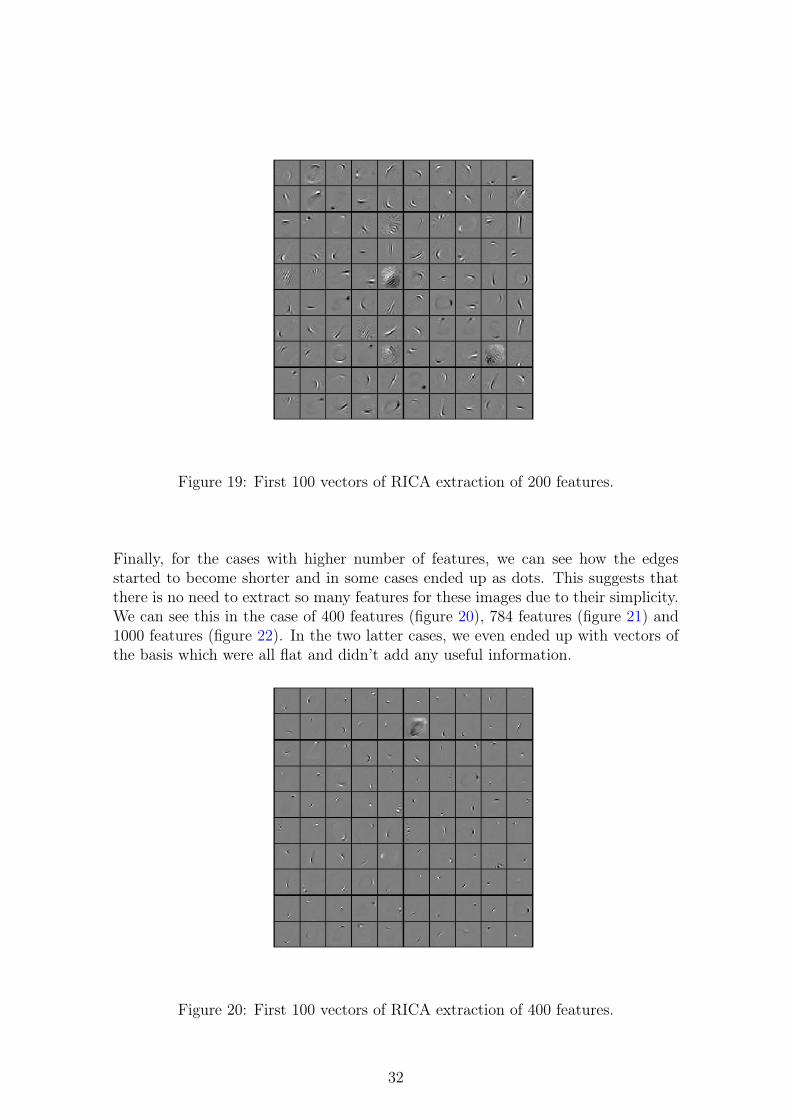
Figure 19: First 100 vectors of RICA extraction of 200 features.

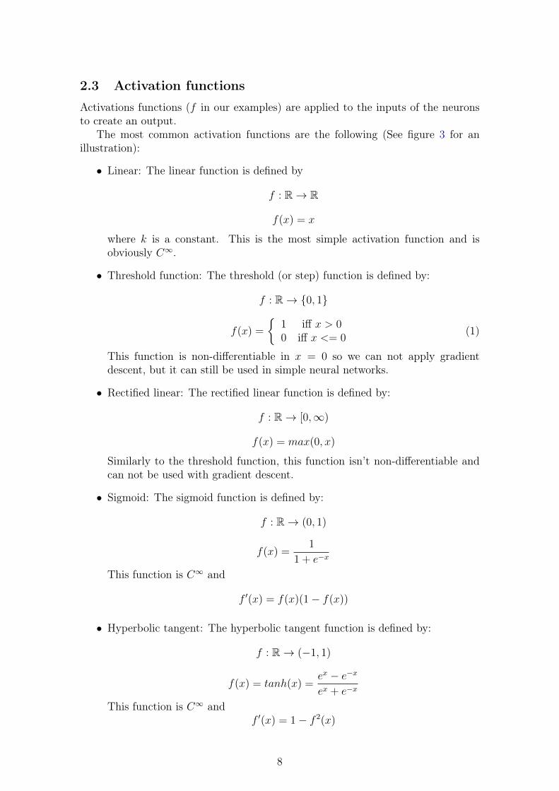
Finally, for the cases with higher number of features, we can see how the edgesstarted to become shorter and in some cases ended up as dots. This suggests thatthere is no need to extract so many features for these images due to their simplicity.We can see this in the case of 400 features (figure 20), 784 features (figure 21) and1000 features (figure 22). In the two latter cases, we even ended up with vectors ofthe basis which were all flat and didn’t add any useful information.

Figure 20: First 100 vectors of RICA extraction of 400 features.

32

Figure 21: First 100 vectors of RICA extraction of 784 features.

Figure 22: First 100 vectors of RICA extraction of 1000 features.

33

To test the accuracy when dealing with the new representation, we trained asoftmax classifier with the images in the different representations. Then, using a setof test images and after transforming them to the new basis, we tested the accuracyof the classification network. Table 3 and figure 23 summarize the results.

Number of features Accuracy of test25 88.5%50 91.1%100 92.0%200 92.8%400 91.4%784 88.9%1000 87.5%

Table 3: Accuracy of tests depending on number of features

Figure 23: Accuracy of tests depending on number of features.

As we can see, the accuracy increased as the number of features increased untilwe reached about 200 features. For more than that, the accuracy started decreasing.This indicates that the images were simple enough that they could be representedwith less dimensions than their number of pixels and that this new representationsgave better results than using more features or even the original images. The fullbasis and the overcomplete basis probably suffered by overfitting and where notuseful for this classification test. Overcomplete basis could be more useful whendealing with larger and more complex images such as fMRI images [16] as the basiswould need to be more complex in order to represent the images accurately.

34

9.3.2 Number of iterations

Whenever we work with a cost function we have to apply an optimization method tofind the desired output. As we have seen, this is the case in RICA, where we applygradient descent to find the optimum W (section 6.3). The process of minimizinga function consists of repeating the iterative algorithm looking for convergence, orthe minimum error possible. Depending on the project, we can choose the stoppingcriterion: by limiting the number of iterations, looking for when the error valuecrosses a given threshold, etc. Intuitively we can understand that the higher thenumber of iterations the more optimum the result will be, but each extra iterationadds computational time to the process which results in longer waits when testing.

In this test, we explored how the performance varies by varying the number ofiterations done by RICA before stopping, and how much time it takes. The rest ofthe variables of the algorithm are kept the same with all the tests, and the numberof iterations will be the only thing that varies. We will test with 100, 500, 1000,5000 and 10000 iterations extracting 100 features. The performance and time takenare summarized in table 4 and in figure 24.

Number of iterations Accuracy of test Time in seconds100 90.3% 44200 91.7% 91500 91.9% 2152000 91.9% 8675000 92.0% 220710000 92.0% 4654

Table 4: Accuracy of tests depending on number of iterations

Figure 24: Accuracy of tests depending on number of iterations.

From this test, we can clearly see that there is a point in which the representationis not going to get any better. In this case, the increase in accuracy going from 500to 10000 is only 0.1%. This reinforces the concept that this application of RICA isa fast converging one.

35

9.3.3 Value of λ

As described in the formulation of RICA in equation (3), there are two parts to theoptimization problem.

λ||Wx||1 + ||W TWx− x||22The first term deals with the sparsity constraint, while the second one looks fora accurate recreation of the original image, by looking for it to be close to therecreation W TWx. The parameter λ defines how much weight we want to give tothe sparsity constraint in relation to the recreation condition. The more weight wegive to the sparsity constraint the less precise will the recreation be, and vice-versa.In table 5 and figure 25 we summarize the accuracy of the classification test whenvarying the value of λ. For these tests, we extracted 100 features with 500 iterationson RICA.

λ Accuracy of test0 91.8%

5× 10−5 91.8%5× 10−4 91.9%5× 10−3 89.7%5× 10−2 66.7%5× 10−1 41.2%

Table 5: Accuracy of tests in relation to λ

Figure 25: Accuracy of tests depending on number of iterations.

From these results, we can reach the conclusion that the recreation constraint ofthe RICA formulation is the most important part and should have the bigger weightwhen optimizing the function in order to find W . However, having no sparsityconstraint did not produce the best results. In fact, we have seen that having asmall sparsity constraint can help prevent degeneration of the basis and thus givebetter performance.

36

9.4 Comparison of PCA, ICA and RICA

In the previous section we have applied RICA to complete images of 28x28 pixels.Unfortunately, as has been explained in section 5.6, ICA requires high computationalpower and time to be applied to big datasets of high-dimensional data. This isusually the case when dealing with images, even so with small images like the onesused previously. Due to the available hardware and time we were not able to performICA on the full set of MNIST images as we have done with RICA. Even though ICAcan not be applied to larger images, it is still tested with small patches of largerimages.

A patch is a small n× n section of an image that is usually extracted randomlyfrom the original dataset. A large number of patches are extracted and ICA can beapplied to them as they are smaller. The representations of the patches extractedwith ICA can be used when applying other algorithms such as convolutional neuralnetworks [13].

9.4.1 Convolution for image processing

Image classification and object recognition are mainly applied to natural images.These types of images are stationary, which means that the statistics of one part ofthe image are the same as for another part of the same image. This allows us touse features extracted from one part of the image in other parts and apply featuredetectors anywhere in the image. To train or create this small feature detector, wecan extract small patches from the original images, and then convolve the featuresextracted with the larger image.

A convolution is done by multiplying the value of a pixel and its neighboringpixels by a matrix. In figure 26 we can see an example of how a 3× 3 patch definedas is convolved to a 5× 5 image.

Figure 26: Example of a convolved feature.

37

9.4.2 Visual comparison of features extracted with ICA and RICA

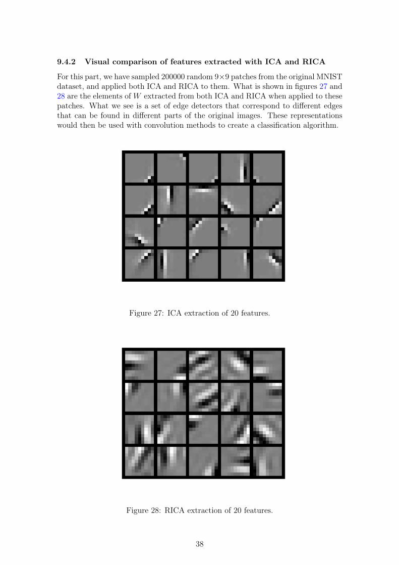
For this part, we have sampled 200000 random 9×9 patches from the original MNISTdataset, and applied both ICA and RICA to them. What is shown in figures 27 and28 are the elements of W extracted from both ICA and RICA when applied to thesepatches. What we see is a set of edge detectors that correspond to different edgesthat can be found in different parts of the original images. These representationswould then be used with convolution methods to create a classification algorithm.

Figure 27: ICA extraction of 20 features.

Figure 28: RICA extraction of 20 features.

38

The main difference between both visualizations is how ICA returns cleaner andsharper edges while RICA returns more blurred ones. This could be due to the fasterconvergence of the FastICA algorithm when compared to the RICA implementation.

9.4.3 PCA

Given that we have studied PCA and have used PCA whitening during this project,we can also take a look at the basis vectors that PCA extracts and see how theycompare to those from ICA and RICA. In figure 29 we can see the first 20 principalcomponents extracted from the same sample of patches as those used in the previoussection.

Figure 29: First 20 Principal Components extracted using PCA

The main difference between this basis and those extracted using ICA and RICAis that in this case we can see how the first vectors of the basis give the mostinformation about the patches, while the rest give less information. Furthermore,using PCA we do not extract independent components as is the case in ICA andRICA.

39

10 Conclusions

10.1 Proposed objectives

The main objective was to review all the different algorithms and methodologiesthat were needed in order to understand Reconstruction ICA, and to create a func-tional implementation so that it could be used for feature extraction tasks. Onceimplemented, this allowed us to study its behavior when varying parameters of theimplementation and to compare the reconstruction with the classical machine learn-ing methods studied during the project. We were able to do this by using a simpledatabase of handwritten digits. The fact that it was comprised of simple and rela-tively small images allowed us to perform many tests in order to evaluate how thealgorithm worked.

10.2 Future work

Future work regarding this project comes from a practical application of the studiedalgorithm. We have tested the implementation and studied its characteristics, buthave not applied it to what would be a more complex problem. The following stepswould be to access a database of complex images such as fMRi scans and analyzingthe results extracted by Reconstruction ICA, and compare them if possible to thoseextracted from ICA. Furthermore, we could study if properties such as overcompletebasis help with classification problems in fMRi, which would show an advantage overusing conventional ICA.

40

References[1] Andrew Ng, Jiquan Ngiam, Chuan Yu Foo, Yifan Mai, Caroline

Suen. Unsupervised Feature Learning and Deep Learning Tutorial.http://ufldl.stanford.edu/tutorial/ Accessed June 2017

[2] Jarrett, K., Kavukcuoglu K., Ranzato, M., i LeCun, Y. What is the best multi-stage architecture for object recognition? IEEE Proc. International Conferenceon Computer Vision. 2009. pp. 2146-2153

[3] Basheera, I. A. i Hajmeerb, M.. Artificial neural networks: fundamentals,com-puting, design, and application. Journal of Microbiological Methods. 2000,Vol.43, pp. 3-31

[4] Jan A. Snyman. Practical Mathematical Optimization: An Introduction toBasic Optimization Theory and Classical and New Gradient-Based Algorithms.Springer Publishing. ISBN 0-387-24348-8

[5] Qiao, Yu (2007). "THE MNIST DATABASE of handwritten digits". RetrievedMay 2017.

[6] Apaar Sadhwani, Apoorv Gupta. Nonlinear Extensions of Reconstruction ICA.2011

[7] Vćlav Hlavć. Principal Component Analysis - Application to images Czech Tech-nical University in Prague

[8] Karhunen J, Oja E, Wang L, Vigario R, Joutsensalo J. A class of neural net-works for independent component analysis IEEE Transactions on Neural Net-works May 1997, 486 - 504.

[9] A. Hyvarinen, E. Oja. Independent Component Analysis: Algorithms and Ap-plications. Neural Networks, 2000, 411-430.

[10] A. Coates, H. Lee, and A. Y. Ng. An analysis of single-layer networks in unsu-pervised feature learning. AISTATS 14, 2011.

[11] G. E. Hinton, S. Osindero, and Y. W. Teh. A fast learning algorithm for deepbelief nets. Neural Computation, 2006.

[12] Quoc V Le, Alexandre Karpenko, Jiquan Ngiam, and Andrew Y Ng. ICA withreconstruction cost for efficient overcomplete feature learning. Advances in Neu-ral Information Processing Systems, 24:1017 - 1025, 2011.

[13] Mattis Paulin, Matthijs Douze, Zaid Harchaoui, Julien Mairal, Florent Per-ronnin, et al.. Local Convolutional Features with Unsupervised Training forImage Retrieval. ICCV 2015 - IEEE International Conference on ComputerVision, Dec 2015, Santiago, Chile. IEEE, pp.91-99

[14] M. Schmidt. minFunc: unconstrained differentiable multivariate optimization inMatlab. http://www.cs.ubc.ca/ schmidtm/Software/minFunc.html, 2005. Ac-cessed June 2017

41

[15] Andrew Ng, Jiquan Ngiam, Chuan Yu Foo, Yifan Mai, CarolineSuen. Unsupervised Feature Learning and Deep Learning Tutorial.http://deeplearning.stanford.edu/wiki/index.php/UFLDL_Tutorial AccessedJune 2017

[16] Calhoun VD, Liu J, Adali T. A review of group ICA for fMRI data and ICAfor joint inference of imaging, genetic, and ERP data. NeuroImage. 2009;45(1Suppl):S163-S172.

42