University of South FloridaScholar Commons

Graduate Theses and Dissertations Graduate School

January 2014

Study of Process Control Strategies for BiologicalNutrient Removal in an Oxidation DitchLeslie Ann KnappUniversity of South Florida, leslie1@mail.usf.edu

Follow this and additional works at: http://scholarcommons.usf.edu/etd

Part of the Environmental Engineering Commons

This Thesis is brought to you for free and open access by the Graduate School at Scholar Commons. It has been accepted for inclusion in GraduateTheses and Dissertations by an authorized administrator of Scholar Commons. For more information, please contact scholarcommons@usf.edu.

Scholar Commons CitationKnapp, Leslie Ann, "Study of Process Control Strategies for Biological Nutrient Removal in an Oxidation Ditch" (2014). GraduateTheses and Dissertations.http://scholarcommons.usf.edu/etd/5249

Study of Process Control Strategies for Biological Nutrient Removal in an Oxidation Ditch

by

Leslie A. Knapp

A thesis submitted in partial fulfillment

of the requirements for the degree of

Master of Science in Civil Engineering

Department of Civil and Environmental Engineering

College of Engineering

University of South Florida

Major Professor: Sarina J. Ergas, Ph.D.

Daniel Yeh, Ph.D.

George Cassady, M.S.

Date of Approval:

June 27, 2014

Keywords: Phosphorus Removal, Simultaneous Nitrification-Denitrification, Mean Cell

Residence Time, Activated Sludge Modeling, BioWin

Copyright © 2014, Leslie A. Knapp

ACKNOWLEDGMENTS

This material is based upon work supported by the National Science Foundation

under Grant No. DUE 0965743. Any opinions, findings, and conclusions or recommendations

expressed in this material are those of the author and do not necessarily reflect the views of the

National Science Foundation.

Many thanks to Dr. Sarina Ergas for her understanding, compassion, and effort. Thank

you to Dr. Daniel Yeh and George Cassady for serving on my committee and helping me along.

Thank you also to Dr. James Mihelcic for his support and allowing me to serve in the Peace

Corps as part of my Master’s degree.

This thesis was possible because of Hillsborough County Public Utilities Department and

the Operations Staff at the Falkenburg Advanced Wastewater Treatment Plant. I greatly

appreciate the willingness of Dan Orlosky, Marcus Moore, and the plant operators and their help

in collecting samples and data. My visits to the WWTP were the highlights of this work.

Many professionals in the wastewater industry generously shared their knowledge and

expertise. Special thanks to engineers from Brown and Caldwell, Gresham, Smith and Partners,

Hazen and Sawyer, and HDR, Inc. for all their help.

Finally, there are many friends who helped me during this time when I needed a ride, a

place to stay, a meal, or someone to talk to. I hope I can return the favor.

i

TABLE OF CONTENTS

LIST OF TABLES ......................................................................................................................... iii

LIST OF FIGURES ....................................................................................................................... iv

ABSTRACT ................................................................................................................................... vi

CHAPTER 1: INTRODUCTION ....................................................................................................1

1.1 Background .....................................................................................................................1

1.2 Research Objectives ........................................................................................................5

CHAPTER 2: LITERATURE REVIEW .........................................................................................6

2.1 Nitrogen Removal ...........................................................................................................6

2.1.1 Simultaneous Nitrification-Denitrification .....................................................8

2.2 Phosphorus Removal .....................................................................................................11

2.2.1 Biological Phosphorus Removal ...................................................................12

2.2.2 Chemical Phosphorus Removal ....................................................................15

2.3 Settling ...........................................................................................................................15

2.3.1 Sludge Bulking..............................................................................................15

2.3.2 Measures of Sludge Quality ..........................................................................16

2.3.3 Sludge Blankets ............................................................................................17

2.4 Process Control for Biological Nutrient Removal ........................................................19

2.4.1 Sources of Variability in WWTPs ................................................................19

2.4.2 Instrumentation, Control, and Analysis ........................................................20

2.4.3 Aeration Control for Simultaneous Nitrification-Denitrification .................21

2.4.4 Wasting Control ............................................................................................22

2.5 Modeling .......................................................................................................................23

2.5.1 Wastewater Characterization and Model Calibration ...................................24

CHAPTER 3: METHODS .............................................................................................................27

3.1 Site Overview ................................................................................................................27

3.2 Following the GMP Unified Protocol Steps ..................................................................28

3.2.1 Step 1: Project Definition..............................................................................29

3.2.2 Step 2: Data Collection and Reconciliation ..................................................29

3.2.3 Step 3: Plant Model Set-up ...........................................................................31

3.2.4 Step 4: Calibration and Validation ................................................................34

3.2.4.1 Wastewater Characterization .........................................................34

3.2.4.2 Goodness of Fit ..............................................................................35

3.2.4.3 Sensitivity Analysis .......................................................................37

3.2.5 Step 5: Simulation and Result Interpretation ................................................37

ii

3.3 Investigation of Phosphorus Removal ...........................................................................38

CHAPTER 4: RESULTS AND DISCUSSION .............................................................................40

4.1 Review of Plant Operation ............................................................................................40

4.1.1 Aeration Control ...........................................................................................41

4.1.2 Wasting Control ............................................................................................41

4.1.3 Data Comparisons between Laboratories .....................................................43

4.2 BioWin Calibration and Validation ...............................................................................45

4.2.1 Wastewater Characterization ........................................................................45

4.2.2 Goodness of Fit .............................................................................................49

4.2.3 Sensitivity Analysis ......................................................................................52

4.2.4 Validation ......................................................................................................53

4.2.5 Simulation and Result Interpretation ............................................................54

4.3 Investigation of Phosphorus Removal ...........................................................................56

CHAPTER 5: CONCLUSIONS AND RECOMMENDATIONS .................................................58

REFERENCES ..............................................................................................................................62

APPENDICES ...............................................................................................................................68

Appendix A List of Acronyms .............................................................................................69

Appendix B Influent Specifier Worksheet ...........................................................................70

Appendix C Distribution of Mass ........................................................................................71

Appendix D Influent Loading ..............................................................................................72

Appendix E Composite Influent and Grab Effluent COD Analyses ...................................73

iii

LIST OF TABLES

Table 3.1 Physical WWTP data .....................................................................................................28

Table 3.2 Assumptions for plant model set-up .............................................................................32

Table 3.3 Combination of kinetic parameters tested during model calibration .............................36

Table 3.4 BioWin COD influent parameters for steady state simulations .....................................38

Table 4.1 Influent TSS and VSS in composite and grab samples ................................................46

Table 4.2 Comparison of literature values to average values of influent parameters from

historical data and supplemental sampling ....................................................................48

Table 4.3 BioWin wastewater fractions .........................................................................................48

Table 4.4 Average sum of absolute residuals of effluent N concentrations with

varying kinetic parameters ............................................................................................49

Table 4.5 BioWin kinetic parameters ............................................................................................50

Table 4.6 Sensitivity analysis for kinetic parameters ....................................................................53

Table 4.7 Average sum of absolute residuals of effluent N concentrations for validation

simulation .......................................................................................................................54

Table E.1 Results from influent and effluent COD analyses. ........................................................73

iv

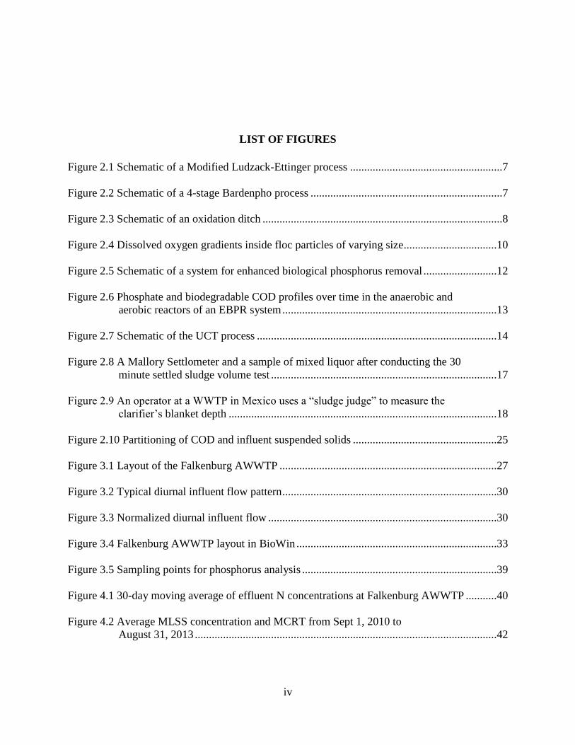
LIST OF FIGURES

Figure 2.1 Schematic of a Modified Ludzack-Ettinger process ......................................................7

Figure 2.2 Schematic of a 4-stage Bardenpho process ....................................................................7

Figure 2.3 Schematic of an oxidation ditch .....................................................................................8

Figure 2.4 Dissolved oxygen gradients inside floc particles of varying size .................................10

Figure 2.5 Schematic of a system for enhanced biological phosphorus removal ..........................12

Figure 2.6 Phosphate and biodegradable COD profiles over time in the anaerobic and

aerobic reactors of an EBPR system ............................................................................13

Figure 2.7 Schematic of the UCT process .....................................................................................14

Figure 2.8 A Mallory Settlometer and a sample of mixed liquor after conducting the 30

minute settled sludge volume test ................................................................................17

Figure 2.9 An operator at a WWTP in Mexico uses a “sludge judge” to measure the

clarifier’s blanket depth ...............................................................................................18

Figure 2.10 Partitioning of COD and influent suspended solids ...................................................25

Figure 3.1 Layout of the Falkenburg AWWTP .............................................................................27

Figure 3.2 Typical diurnal influent flow pattern ............................................................................30

Figure 3.3 Normalized diurnal influent flow .................................................................................30

Figure 3.4 Falkenburg AWWTP layout in BioWin .......................................................................33

Figure 3.5 Sampling points for phosphorus analysis .....................................................................39

Figure 4.1 30-day moving average of effluent N concentrations at Falkenburg AWWTP ...........40

Figure 4.2 Average MLSS concentration and MCRT from Sept 1, 2010 to

August 31, 2013 ...........................................................................................................42

v

Figure 4.3 Concentration of total phosphorus, ammonia, and nitrate measured in the

final effluent by the County lab and in filtered mixed liquor at the

effluent of the oxidation ditch measured by operators in the plant lab. ........................44

Figure 4.4 COD results from wastewater characterization ............................................................45

Figure 4.5 Total and filtered influent COD ...................................................................................47

Figure 4.6 Total and volatile influent suspended solids ................................................................47

Figure 4.7 Total and reactive influent phosphorus ........................................................................47

Figure 4.8 Observed and modeled MLSS concentration ...............................................................50

Figure 4.9 Observed and modeled MLVSS concentration ............................................................51

Figure 4.10 Observed and modeled effluent TKN concentration ..................................................52

Figure 4.11 Influent TKN mass load .............................................................................................52

Figure 4.12 Response of MLSS concentration to changing SRT during steady state

simulations with constant influent parameters and aeration regimen. .......................55

Figure 4.13 Response of effluent ammonia concentration to changing SRT during

steady state simulations with constant influent parameters and aeration

regimen. ......................................................................................................................55

Figure 4.14 Response of MLSS concentration to changing influent COD concentration

during steady state simulations with constant SRT and aeration regimen ................56

Figure 4.15 Response of effluent ammonia and nitrate concentrations to changing

influent COD concentration during steady state simulations with constant

SRT and aeration regimen. ........................................................................................56

Figure 4.16 Reactive phosphorus profile from grab samples taken throughout the

treatment process .......................................................................................................57

Figure B.1 BioWin influent specifier worksheet ...........................................................................70

Figure C.1 Percent distribution of mass between clarifier, selector, and oxidation ditch .............71

Figure D.1 Mass load of influent COD calculated from a 24-hour sampling event ......................72

Figure D.2 Mass load of influent phosphorus calculated from a 24-hour sampling event ............72

Figure D.3 Mass load of influent TSS and VSS calculated from a 24-hour sampling event ........72

vi

ABSTRACT

Advanced wastewater treatment plants must meet permit requirements for organics,

solids, nutrients and indicator bacteria, while striving to do so in a cost effective manner. This

requires meeting day-to-day fluctuations in climate, influent flows and pollutant loads as well as

equipment availability with appropriate and effective process control measures. A study was

carried out to assess performance and process control strategies at the Falkenburg Road

Advanced Wastewater Treatment Plant in Hillsborough County, Florida.

Three main areas for control of the wastewater treatment process are aeration, return and

waste sludge flows, and addition of chemicals. The Falkenburg AWWTP uses oxidation ditches

where both nitrification and denitrification take place simultaneously in a low dissolved oxygen,

extended aeration environment. Anaerobic selectors before the oxidation ditches help control the

growth of filamentous organisms and may also initiate biological phosphorus removal. The

addition of aluminum sulfate for chemical phosphorus removal ensures phosphorus permit limits

are met. Wasting is conducted by maintaining a desired mixed liquor suspended solids (MLSS)

concentration in the oxidation ditches.

For this study, activated sludge modeling was used to construct and calibrate a model of

the plant. This required historical data to be collected and compiled, and supplemental sampling

to be carried out. Kinetic parameters were adjusted in the model to achieve simultaneous

nitrification-denitrification. A sensitivity analysis found maximum specific growth rates of

nitrifying organisms and several half saturation constants to be influential to the model.

vii

Simulations were run with the calibrated model to observe relationships between sludge age,

MLSS concentrations, influent loading, and effluent nitrogen concentrations.

Although the case-study treatment plant is meeting discharge permit limits, there are

several recommendations for improving operation performance and efficiency. Controlling

wasting based on a target MLSS concentration causes wide swings in the sludge age of the

system. Mixed liquor suspended solids concentration is a response variable to changes in sludge

age and influent substrate. Chemical addition for phosphorus removal could also be optimized

for cost savings. Finally, automation of aeration control using online analyzers will tighten

control and reduce energy usage.

1

CHAPTER 1: INTRODUCTION

1.1 Background

Amendments to the Clean Water Act in 1972 established a system of permitting for point

source discharges to surface water bodies in the United States (EPA, 2002). This permitting

system, known as the National Pollutant Discharge Elimination System (NPDES), applies to

wastewater treatment plants (WWTPs) that treat municipal and industrial wastewater. Generally,

the issuing of permits is the responsibility of state regulatory agencies, and each WWTP must

apply for and receive a specific permit tailored to the individual facility based on the

characteristics of the receiving water body. At a minimum, most WWTPs must meet permit

requirements for organics, solids, and indicator bacteria. Stricter permits limit the amount of

nutrients, namely nitrogen (N) and phosphorus (P), that may be discharged, and these stricter

permits require design and operation of advanced wastewater treatment plants (AWWTPs) that

have additional treatment technologies.

Complying with permit limits requires meeting day-to-day fluctuations in influent flows,

pollutant loads, temperature, and equipment availability with effective process control measures.

Design engineers strive to create appropriate and robust treatment systems; however, the

performance of WWTPs is ultimately dependent on the operating practices and decisions made

by treatment plant operators and managers. In addition to legally complying with NPDES

permits, many WWTPs are focusing on reducing carbon footprints and even becoming energy

neutral or net-energy positive (Schwarzenbeck et al., 2008; Mo and Zhang, 2012; Gori et al.,

2013; Jenicek et al., 2013). As the level of treatment needed to meet stricter N and P limits

2

increases, the emissions of greenhouse gases and other air pollutants associated with energy and

chemical usage also increases (Falk et al., 2011). Process monitoring and control is critical to

efficient operation that will save energy and decrease operating costs while ensuring that the

requirements of discharge permits are met.

Throughout 2013 and 2014, special conferences are being held to celebrate the 100th

anniversary of the activated sludge process for the treatment of wastewater. The term activated

sludge refers to wastewater that has been aerated to allow for the growth of microorganisms that

consume soluble organic matter (Grady et al., 1999). Modifications to the activated sludge

process can be made to achieve biological nutrient removal (BNR) of N and P. The following

excerpt is from a study published in 1914 by Ardern and Lockett, who are credited with the

development of the activated sludge process.

“The main feature of the experimental work was the satisfactory purification

of sewage by tank treatment alone, with the production of a sludge, which

owing to its oxidised and flocculent condition, could be readily dealt with and

turned into a valuable fertilising agent.” –(Ardern and Lockett, 1914)

This excerpt highlights two important functions of the activated sludge process that

operators are attempting to control: transformation of wastewater constituents through oxidation

(and reduction) and the ability of activated sludge bacteria to flocculate and settle. Mixed liquor

suspended solids (MLSS) is the term given to the solids in the biological treatment system and

refers to the mixture of newly formed solids and settled solids that are returned to the reactor.

Generally, there are three main areas where the treatment plant operator makes adjustments to

control the activated sludge process: 1) aeration and mixing, 2) return and waste sludge flows,

and 3) chemical addition. Operators collect samples, perform tests, use readings from online

analyzers and meters, and analyze data to determine how the plant is performing and what

actions need to be taken to achieve desired performance. While knowledge of the activated

3

sludge processes has greatly increased over the past 100 years, continual efforts to minimize

plant upsets and increase efficiency are still needed.

Because the operator is ultimately responsible for the performance and efficiency of the

WWTP, operator training and the information disseminated for process control is paramount.

The Office of Water Programs (OWP) at California State University of Sacramento received a

federal grant in 1968 to establish a correspondence training program for wastewater treatment

plant operators (Austin et al. 1970). For the past four decades, OWP has been providing

correspondence courses and training manuals, colloquially known as “the Sacramento Manuals”,

for all levels of WWTP operator. The Sacramento Manuals have been widely used over the

years, with most states listing them as approved training material to qualify operators to sit for

required certifying exams. The content of these manuals has gone largely unchanged since their

inception, and while much effort has been made to be operator-friendly, some information is

contradictory to other literature and reference texts. For example, Volume II of the Operation of

Wastewater Treatment Plants manual (OWP, 2008) states: “Usually, it is necessary to vary the

amount of MLSS in the ditch as seasons change. Because the microorganisms are not as active

in winter at low temperatures, the MLSS will need to be higher in the winter than in the summer

if complete nitrification is desired.” In contrast, other reference materials and researchers stress

that the nitrifying biomass is dependent on only two variables: mean cell residence time (MCRT)

and the average ammonia load (Grady et al. 1999; Rieger et al., 2014). Another Sacramento

Manual, Advanced Waste Treatment (OWP, 2006), states “The operator is usually working with

a fixed reactor volume and will need to determine the desired MLSS concentration and overall

MCRT to meet one or more treatment objectives”. This implies that the MCRT and the MLSS

concentration may be controlled at the same time. Neglecting the MCRT by focusing on

4

increasing MLSS concentration may result in poor sludge quality leading to negative effects on

sludge flocculation, settling, and compaction.

Advancements in computer technology, data storage, and sensor capability have made it

possible to easily store and retrieve large quantities of data. Some data collection and reporting

is mandatory for permitting requirements, while other data are collected for in-plant process

control purposes. Data collection is an attempt to come as close as possible to understanding the

processes occurring in the WWTP. Data must also be as accurate as possible to be truly

representative. Potential error in data collection can be determined using mass balances (Puig et

al, 2008), comparisons of parameter ratios and ranges, and statistical tests. Graphing of data can

also be used to quickly visualize outlying values. While sampling and laboratory analysis are

essential to the successful operation, time and cost factors must be considered when choosing the

appropriate sampling regimen.

Technological advancements have also contributed to the development and increased use

of mathematical models of the activated sludge system, which can be powerful tools for the

design and operation of WWTPs. Mathematical models use equations that represent the uptake

and conversion of substrates by bacteria, as well as physical processes such as sedimentation and

chemical precipitation. The International Water Association (IWA) published Activated Sludge

Model 1 (ASM1) in 1987, which set the stage for the evolution of more complex models that

simulate nitrogen and phosphorus removal processes. An indirect benefit of modeling is that the

use of ASM models has highlighted existing gaps in research and helped to guide scientific

investigation of wastewater treatment processes. In addition to the knowledge gained from

running simulations to test varying conditions, the need for ample and accurate data used in

5

model construction and calibration can also help draw attention to existing errors at individual

WWTPs (Henze et al., 2000).

1.2 Research Objectives

The overall goal of this project is to improve operator knowledge, process control and

system performance using analysis of historical data and activated sludge modeling at a full-

scale AWWTP. Specific objectives are to:

Investigate process control best practices for advanced wastewater treatment plants and their

applicability to the case-study AWWTP;

Analyze influent, effluent and operating data over a three-year period (September 1, 2010 to

August 31, 2013) to further understand process performance, determine gaps in knowledge,

and suggest possible improvements for future data collection;

Construct and calibrate a BioWin model of the plant following published guidelines for good

modeling practice;

Use the calibrated plant model to simulate the effect of changes in MCRT and influent

pollutant loads on plant performance.

6

CHAPTER 2: LITERATURE REVIEW

This literature review focuses on nutrient removal processes, process control strategies,

and modeling of activated sludge systems. Specific attention was given to oxidation ditches to

highlight the case study WWTP.

2.1 Nitrogen Removal

Nitrification and denitrification are widely used biological processes for the removal of

nitrogen from wastewater. Nitrification is understood to occur under aerobic conditions, where

predominately autotrophic bacteria oxidize ammonia to nitrite and then nitrate using oxygen as

an electron acceptor. Denitrification occurs when heterotrophic bacteria reduce nitrate to

nitrogen gas under anoxic conditions (absence of free oxygen). Denitrifying bacteria will use

oxygen as an electron acceptor in preference to nitrate because it is more thermodynamically

favorable, thus making anoxic conditions imperative for denitrification to take place. The

overall reactions for nitrification and denitrification are given in equations [1] and [2] (Henze et

al, 2002).

Autotrophic oxidation of ammonium:

[1]

Heterotrophic reduction of nitrate (with ammonia assimilation for growth):

[2]

These equations show that alkalinity, in the form of HCO3-, is consumed during nitrification.

This is important because nitrifiers will be inhibited at low pH. Some alkalinity is recovered

during denitrification.

7

A number of different treatment plant configurations have been invented and successfully

implemented for nutrient removal over the years. Some systems, such as the Modified Ludzack-

Ettinger (MLE) and Bardenpho ® processes, provide dedicated zones or tanks for nitrification

and denitrification (Barnard, 1975; Ludzack and Ettinger, 1962). The MLE process (Figure 2.1)

consists of an anoxic zone followed by an aerated zone. Internal mixed liquor recycle returns

nitrified mixed liquor to the anoxic zone, where the influent wastewater provides carbon for the

denitrifying bacteria. The 4-stage Bardenpho configuration (Figure 2.2) consists of an

anoxic/aerobic layout similar to the MLE process, with an additional anoxic (and optional

external carbon source) and aerobic zones for further nitrogen removal and sludge conditioning.

Figure 2.1 Schematic of a Modified Ludzack-Ettinger process.

Figure 2.2 Schematic of a 4-stage Bardenpho process.

The term “oxidation ditch” is used loosely to refer to a variety of operating schemes and

physical configurations. In general, all oxidation ditch systems are loop-shaped reactors

operated in an extended aeration mode at relatively long hydraulic retention time (HRT) and

8

MCRT (Mandt and Bell, 1982). Operating with a longer MCRT makes nitrification possible

even at low dissolved oxygen (DO) levels (Stenstrom and Poduska, 1980). The oxidation ditch

is typically configured in a race-track style, with mechanical aerators or brushes placed at one or

more points along the ditch. Mechanical aeration entrains oxygen and provides mixing in a

horizontal flow pattern around the ditch. This flow pattern allows the mixed liquor to be

recirculated around the ditch, presumably between aerobic and anoxic zones. Oxidation ditches

exhibit simultaneous nitrification and denitrification, which will be discussed in detail in the next

section. A schematic of a single-pass Carrousel oxidation ditch is shown in Figure 2.3.

Figure 2.3 Schematic of an oxidation ditch.

Because nitrification and denitrification are occurring concurrently in an oxidation ditch,

the consumption of alkalinity by nitrifying bacteria is partially offset by the alkalinity production

of denitrifiers. The circular flow pattern in the ditch also supplies denitrifying bacteria with

influent carbon and nitrate without the need for supplemental carbon addition or internal mixed

liquor recycle. Oxidation ditches are sometimes paired with additional reactors to create

Bardenpho or other type systems, so attention should be given to the exact nature of the WWTP.

2.1.1 Simultaneous Nitrification-Denitrification

Although many operating schemes use separate basins for aerobic and anoxic processes,

substantial denitrification has been observed in aerated bioreactors without dedicated anoxic

Oxidation Ditch

Secondary Clarifier

RAS WAS

Effluent Influent

Mechanical Aerator

9

zones. In fact, the observation of denitrification within the aeration basin was the impetus for the

creation of specific zones for nitrification and denitrification in an attempt to enhance removal

rates (Barnard, 1998; Ludzack and Ettinger, 1962). The occurrence of nitrification and

denitrification at the same time in a single reactor without distinct aerated and non-aerated zones

is commonly referred to as simultaneous nitrification-denitrification (SND). Treatment systems

exhibiting SND typically have relatively long SRTs, aeration equipment that creates non-uniform

flows, such as mechanical aerators, and an operating procedure to limit oxygen input (Daigger,

2013). Recently, some WWTPs that were designed with separate aerobic and anoxic zones have

been reconfigured to lower the DO concentration within the aerobic portion of the system to

achieve high levels of SND (Jimenez et al, 2010; 2013). Operating at low DO concentrations has

the potential to decrease overall energy usage, as supplying oxygen is often the most costly and

energy-intensive process in the WWTP (WEF, 2010).

Three mechanisms for the occurrence of SND have been investigated previously

(Daigger et al., 2007): (1) occurrence of aerobic and anoxic zones within the reactor, (2)

occurrence of aerobic and anoxic zones within the floc particle, and (3) existence of novel

microorganisms with alternative biochemical pathways. The literature is inconclusive as to

whether the macro environment, the presence of aerobic and anoxic zones within the reactor,

plays an important role in SND processes. Rittmann and Langeland (1985) measured DO,

nitrate, and nitrite concentrations in full-scale Carrousel oxidation ditches. The authors found

that denitrification occurred continuously in the reactor without evidence of distinct anoxic

zones. Dissolved oxygen profiles in an Orbal oxidation ditch showed low DO concentrations

(0.2 mg/L) before and after the mechanical aerator, suggesting that a DO gradient within the floc

instead of heterogeneity in the reactor was the principal mechanism for SND (Daigger and

10

Littleton, 2000). Although difficult to measure in the field, a later study of the same Orbal

reactor using computational fluid dynamics suggested that areas of higher and lower DO

concentration can occur (Littleton et al., 2007).

In regards to the micro-environment in SND reactors, a study comparing SND

performance with varying floc particle size found denitrification diminished with smaller floc

sizes, possibly due to the diffusion of oxygen into the inner areas of the floc (Pochana and

Keller, 1999). Daigger et al. (2007) further investigated DO gradients within individual floc

particles using a “microprobe”. The concentration of DO within floc particles decreased steadily

with depth and ultimately reached near-zero levels in the interior of the larger flocs (≥ 2mm), as

shown in Figure2.4.

Figure 2.4 Dissolved oxygen gradients inside floc particles of varying size.

Nitrite Shunt refers to the conversion of ammonia to nitrogen gas without the

intermediary step of the oxidation of nitrite to nitrate. Instead, ammonia is oxidized to nitrite,

11

and nitrite is directly reduced to nitrogen gas by anoxic heterotrophic or autotrophic metabolism.

Operating at low DO may result in limited nitrification and the occurrence of nitrite shunt (Ju et

al., 2007). Littleton et al. (2003) further investigated the role of novel microorganisms in SND

and found the contribution of alternative biochemical pathways to nitrification/denitrification to

be insignificant.

In a typical nitrification reactor, blower or mechanical aerator speed is increased in

response to an increase in ammonia concentration. However in a single reactor with SND,

increasing the DO concentration will ultimately inhibit denitrification. Therefore, maintaining

sufficient DO for nitrification without negatively impacting denitrification is critical. A bulk DO

concentration of 0.4-0.5 mg/L has been found to be optimal for SND (Münch et al, 1996; Insel,

2007; Dey, 2010), with a decrease in denitrification rate occurring at greater than 0.8 mg/L

(Pochana and Keller, 1999). Because diffusion of oxygen into the floc particle is one of the

mechanisms of SND, the optimal bulk DO concentration may be dependent on the size and

characteristics of the floc, as discussed previously. Another factor that may be especially

influential on the rate of denitrification is the shearing of floc particles by mechanical aerators

(Barnard et al., 2004). As the mixed liquor comes into contact with the aerator, the shearing of

the floc allows carbon necessary for denitrification to be absorbed before re-flocculation takes

place.

2.2 Phosphorus Removal

If NPDES permits set limits for phosphorus, treatment systems for phosphorus removal

must be implemented. While complete chemical removal of nitrogen is usually prohibited by

cost, phosphorus is commonly removed by a combination of both chemical and biological

processes. Biological phosphorus removal is less reliable and understood than other nutrient

12

removal processes, and addition of chemical removal processes is often needed to ensure permit

compliance (Ingildsen et al., 2006; Oehmen et al., 2007).

2.2.1 Biological Phosphorus Removal

Phosphorus is essential to life, making up important molecules such as adenosine

triphosphate (ATP), DNA and RNA, and the phospholipids that form cellular membranes. While

all bacteria in the activated sludge process must have sufficient amounts of phosphorus to meet

energy and growth needs, some species of bacteria can take up more phosphorus than needed for

metabolism. Many species appear to be capable of excess uptake of phosphorus (Mino et al.,

1998, Bond et al., 1999) and these bacteria are collectively called phosphorus accumulating

organisms (PAOs). Enhanced biological phosphorus removal (EBPR) is the term given to

treatment systems that take advantage of the phosphorus accumulation by PAOs. Generally, the

design of EBPR systems includes an anaerobic zone followed by an aerobic zone as shown in

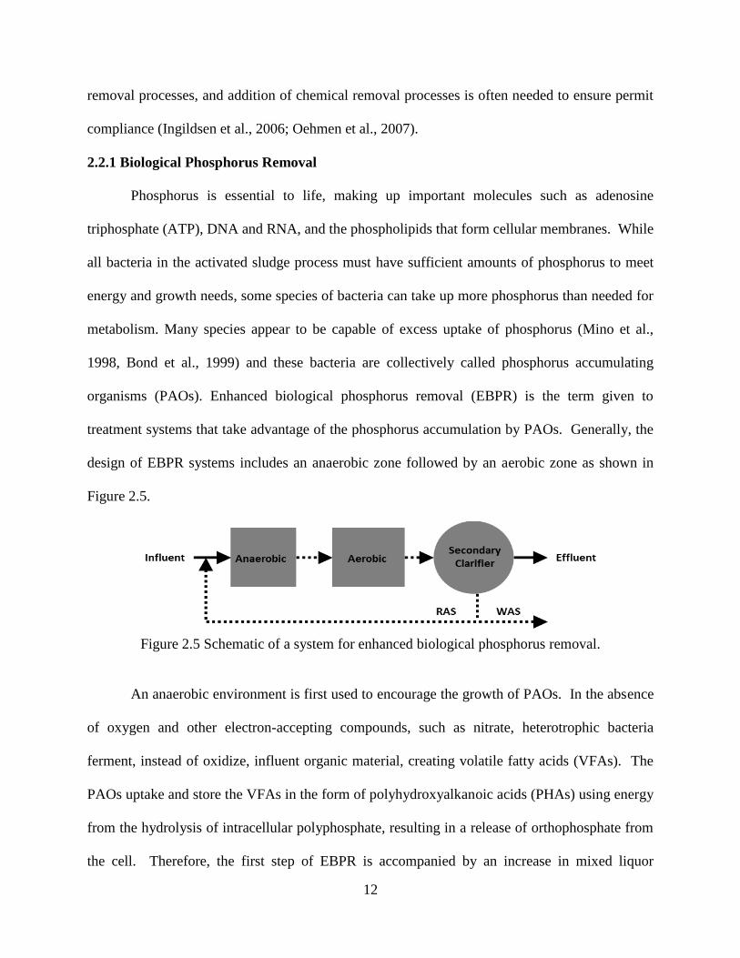
Figure 2.5.

Figure 2.5 Schematic of a system for enhanced biological phosphorus removal.

An anaerobic environment is first used to encourage the growth of PAOs. In the absence

of oxygen and other electron-accepting compounds, such as nitrate, heterotrophic bacteria

ferment, instead of oxidize, influent organic material, creating volatile fatty acids (VFAs). The

PAOs uptake and store the VFAs in the form of polyhydroxyalkanoic acids (PHAs) using energy

from the hydrolysis of intracellular polyphosphate, resulting in a release of orthophosphate from

the cell. Therefore, the first step of EBPR is accompanied by an increase in mixed liquor

13

dissolved phosphorus concentrations. The removal of phosphorus occurs in the subsequent

aerobic stage, when PAOs oxidize stored PHA using oxygen or nitrate as an electron acceptor.

Oxidation of PHA is accompanied by uptake of the phosphate that was released along with

additional phosphorus that was present in the raw influent wastewater. Phosphorus removal is

accomplished when sludge is wasted from the system. Figure 2.6 shows the expected profile of

phosphate and soluble, biodegradable COD over time through the anaerobic and aerobic reactors

designed for EBPR.

Figure 2.6 Phosphate and biodegradable COD profiles over time in the anaerobic and aerobic

reactors of an EBPR system.

If nitrate is present in the RAS that enters the anaerobic zone, denitrifiers may

outcompete PAOs and hinder EBPR. Several process configurations have been developed to

over-come this problem. For example, the University of Cape Town (UCT) process eliminates

the presence of nitrate in the anaerobic reactor by returning settled sludge to the anoxic tank and

supplying microbes to the anaerobic reactor through internal anoxic mixed liquor recycle as

shown in Figure 2.7.

14

Figure 2.7 Schematic of the UCT process.

Although EBPR systems are designed with aerobic zones for phosphorus uptake, at least

some PAOs can use nitrate as an electron acceptor during phosphorus uptake (Hu et al., 2002;

Mino et al., 1998; Stevens et al., 1999). Substantial removal of phosphorus has also been

observed in systems without anaerobic-aerobic configurations. Jimenez et al. (2010) observed

significant removal of phosphorus (93.75%), without chemical addition, in a pilot plant operated

at low DO for SND without a dedicated anaerobic stage. Removal of phosphorus was also

observed in Orbal oxidation ditch reactors at full-scale plants without dedicated anaerobic zones

or chemical addition (Daigger and Littleton, 2000). The authors suggested that mixing patterns

may create anaerobic areas within the Orbal reactor, but that any anaerobic areas existing within

the floc would likely not receive diffused readily biodegradable organic material. A CFD model

of the same Orbal oxidation ditch reactor demonstrated the occurrence of varying DO

environments that could result in anaerobic zones where PAOs could compete with other

heterotrophs (Littleton et al., 2007).

Clarifier design and operating conditions can have an impact on the performance of

EBPR systems. There is potential for a secondary release of phosphorus in the secondary

clarifier if settled sludge is subject to anaerobic conditions in the absence of VFAs (Mikola et al.,

15

2009). Effluent phosphorus concentration will also be impacted if suspended solids escape over

the clarifier weir due to poor settling.

2.2.2 Chemical Phosphorus Removal

Phosphorus removal can also be achieved with the addition of chemicals at different

stages of the treatment process, such as in the primary clarifier or the mixed liquor for

precipitation in the secondary clarifiers. Ferric chloride and aluminum sulfate (alum) are

examples of metal salts that are added to wastewater to precipitate phosphorus. The optimal

dosage is usually determined on-site with jar tests and is dependent on the species of phosphorus

present and the plant permit requirements (WEF, 2011). Bowker and Stensel (1990) point out

that increased sludge production and effect on thickening and dewatering characteristics of

sludge are two considerations when using aluminum salts for phosphorus removal.

2.3 Settling

The ability of bacteria to flocculate and settle is a necessary component of suspended

growth activated sludge treatment systems. Mixed liquor suspended solids settle in the

secondary clarifier and are returned to the aeration basin or wasted. Poor settling mixed liquor

will decrease the capacity of the secondary clarifiers and may result in excessive loss of solids

over the weirs in the secondary effluent. Sludge Volume Index (SVI) is commonly used as a

measure of sludge flocculation and settling ability.

2.3.1 Sludge Bulking

Sludge bulking caused by filamentous organisms is a frequently-encountered problem in

activated sludge systems, resulting in poor settling sludge in the secondary clarifier. Defining the

exact conditions responsible for the proliferation and control of filamentous organisms can be

difficult, as bulking occurs at numerous plants with a range of operating conditions (Ekama and

16

Wentzel, 1999). WWTPs that operate at low DO, long MCRTs, and low F:M ratios are

particularly susceptible to filamentous bulking (Jenkins et al., 1993). In addition to achieving

nutrient removal goals, manipulating reactor environments also serves to promote the growth of

floc-forming organisms and reduce the population of filamentous organisms. Control of bulking

uses some of the same principles as those used in the design of EBPR systems. In fact, an

anaerobic reactor for EBPR is considered to be a selector, and PAOs are classified as floc-

forming bacteria (Grady et al., 1999). A selector tank is introduced before the main aeration

reactor to create feed-starve conditions, taking advantage of readily available organic matter.

Filamentous organisms have been found to be less able than floc-formers to store substrate

during the “feed” stage for subsequent use in the “starve” stage (van Niekerk et al., 1989).

Chlorine can also be added to RAS to temporarily reduce the population of filamentous

organisms, although this practice has had negative effects on biological phosphorus removal

(Diagger et al., 1988). Microscopic examination of the mixed liquor can confirm the presence of

filaments, and resources are available to help with identification of the particular species and

type of filament present (Jenkins et al., 1993).

2.3.2 Measures of Sludge Quality

Although good sludge quality, activated sludge that flocculates, settles, and compacts, is

critical for the successful operation of the WWTP, its measurement varies between plants.

Sludge Volume Index (SVI) is a regularly calculated value by wastewater treatment operators in

attempt to determine sludge quality, and it is used as an indirect indicator of bulking sludge. To

calculate SVI, a sample of mixed liquor is first collected and allowed to settle for 30 minutes in a

“settlometer” (Figure 2.8). Then, the height of the settled sludge is measured, divided by the

17

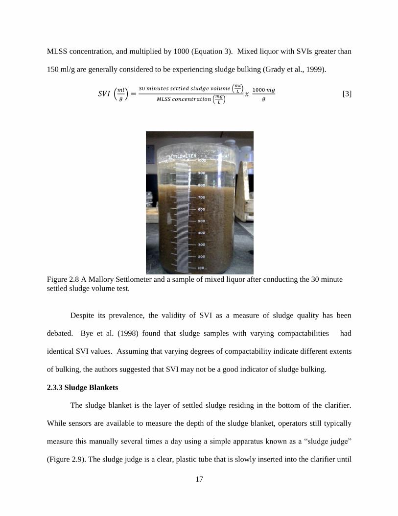
MLSS concentration, and multiplied by 1000 (Equation 3). Mixed liquor with SVIs greater than

150 ml/g are generally considered to be experiencing sludge bulking (Grady et al., 1999).

(

)

(

)

(

)

[3]

Figure 2.8 A Mallory Settlometer and a sample of mixed liquor after conducting the 30 minute

settled sludge volume test.

Despite its prevalence, the validity of SVI as a measure of sludge quality has been

debated. Bye et al. (1998) found that sludge samples with varying compactabilities had

identical SVI values. Assuming that varying degrees of compactability indicate different extents

of bulking, the authors suggested that SVI may not be a good indicator of sludge bulking.

2.3.3 Sludge Blankets

The sludge blanket is the layer of settled sludge residing in the bottom of the clarifier.

While sensors are available to measure the depth of the sludge blanket, operators still typically

measure this manually several times a day using a simple apparatus known as a “sludge judge”

(Figure 2.9). The sludge judge is a clear, plastic tube that is slowly inserted into the clarifier until

18

it reaches the bottom and then pulled back out. A check valve in the bottom of tube traps the

contents of the clarifier inside, essentially taking a core sample. The height of the sludge blanket

inside the tube is measured and recorded.

Figure 2.9 An operator at a WWTP in Mexico uses a “sludge judge” to measure the clarifier’s

blanket depth.

If blankets are allowed to accumulate, the clarifier will eventually fail and solids will exit

over the clarifier weirs with the secondary effluent. This “wash out” scenario is particularly

likely during high flow events. In general, suggested blanket levels are between 0 and 3 feet

(WEF, 2002). Sludge blankets can also result in rising sludge. Nitrate present in the sludge

blanket can undergo denitrification due to the development of anoxic conditions. The

subsequent release of nitrogen gas to the surface of the clarifier can cause sludge to rise.

Rerelease of phosphorus may also occur due to absence of oxygen within the blanket. Unlike the

phosphorus release that takes places in the anaerobic tank before aeration, phosphorus released

within the blanket will not undergo re-uptake.

19

2.4 Process Control for Biological Nutrient Removal

Many textbooks and trade manuals on wastewater treatment highlight the importance of

process control and attempt to outline and define the process control strategies that are available

to the wastewater treatment plant operator. In general, the three main operational areas for the

control of the activated sludge process are return activated sludge flow, waste activated sludge

flow, and dissolved oxygen concentration. Manipulation of internal recycle flows and the

addition of external sources of carbon may also be considered in process control strategies but

will not be addressed here due to the characteristics of the oxidation ditch technology.

2.4.1 Sources of Variability in WWTPs

Wastewater treatment plants are subject to many sources of variability. Influent flows

and loads fluctuate diurnally, weekly, and seasonally. More sporadic fluctuations in flow may

result from pumping at lift stations in the collection system or during periods of high flow

variability, such as large sporting events or heavy rains. Periodic discharges of industrial

wastewater, septage or landfill leachate can greatly alter the loading to the plant. To comply

with NPDES permits and gain insight into plant operation, grab and 24-hour composite samples

are collected and analyzed in certified on-site or contracted laboratories. Variability in plant data

could result from something as simple as poor sample collection if an operator fails to

sufficiently agitate the composite-sample container before collecting the sample. The results of a

bench-top analysis in a mixed liquor sample may be grossly misrepresentative if the operator lets

too much time pass before filtering the sample as the bacteria will continue to act on the

constituents of interest.

Knowledge about the WWTP process can be gained from datasets using a variety of

visual and statistical methods. First, the integrity of data can be assessed using simple “common

20

sense” checks. For example, the MLVSS can never be higher than the MLSS. While it may be

easy to spot an unusually high or low value in a dataset, determining if the outlier represents a

true value can be difficult. Examining ratios of parameters (COD/total phosphorus, BOD/TSS,

COD/TKN) can aid in identifying erroneous outliers (Bratby and Fevig, 2012). If a flow meter

does not accurately measure the rate of WAS wasted daily, calculation of MCRT will be

inaccurate. Conducting mass balances will expose discrepancies in data such as the amount of

sludge wasted that would ultimately affect the calculation of MCRT. For example, the influent

loading of phosphorus should equal the phosphorus in the effluent and the WAS.

2.4.2 Instrumentation, Control, and Analysis

Arthur (1983) lists three key factors for effective process control: (1) controllability of

plant components, (2) capable on-line sensors, and (3) management of data. Controllability of

plant components refers to the ability to make adjustments to aeration equipment, RAS, and

wasting. For example, control may be limited by the available speeds (both minimum and

maximum) of aerators or if wasting is hindered by downstream processes such as dewatering.

On-line analyzers must be dependable and produce quality data. Finally, the performance of the

system must be assessed using data collected by operators and analyzers in order to make

process control decisions. In addition to these factors, the setting of priorities, such as

minimizing cost and meeting effluent requirements, will help to guide the plant operator

There are many types of on-line sensors on the market today, and their reliability is

continually improving. While this study will not investigate different sensors, it should be noted

that there are sensors available for measuring operating parameters such as oxidation-reduction

potential (ORP), MLSS, ammonia, nitrate and DO concentration. Myers et al. (2006) found that

ORP probes are effective to control aeration and ammonia concentration in an extended aeration

21

oxidation ditch. ORP-probes measure the ability of a solution to accept or donate electrons, and

may be particularly useful in low-DO extended aeration processes.

Olsson et al. (1999) list four components of control for wastewater systems: the process,

the measurement, the decision-making, and the implementation. These components are arranged

depending on whether the control is feedback or feedforward. In feedback control, a

“disturbance” is measured after it affects the process, and decisions and adjustments are made

accordingly to correct the impact of the disturbance. Feedforward control involves measuring

disturbances directly before they impact the process and making decisions and implementations

to the process that will off-set or eliminate the disturbance. Both feedback and feedforward

control can be used to improve process stability, reduce operating costs, and ensure permit

compliance.

2.4.3 Aeration Control for Simultaneous Nitrification-Denitrification

Jimenez et al. (2013) investigated and compared two aeration control strategies (constant

low DO and ammonia-based control) for SND in bench scale sequencing batch reactors (SBRs)

and at several full-scale WWTPs. For the bench scale experiment, two SBRs were operated in

parallel. The bulk DO concentration in one of the SBRs was maintained at a constant low DO of

between 0.25 and 0.5 mg/L. In the second SBR, ammonia was monitored and aeration was

turned off and on when the ammonia concentration reached 0.5 and 1.0 mg/L, respectively, with

a maximum DO set point of 0.8 mg/L. The performance (% removal of nitrogen) of both

strategies was compared, with constant low DO producing lower TN values overall but with

higher SVI values. A comparison of eight full-scale WWTPs using either constant low DO or

ammonia-based control for SND showed that both strategies produced good nitrogen removal,

22

but ammonia-based control resulted in better sludge quality (lower SVI values). However, the

authors noted that other variables, such as sludge age, were not taken into account.

2.4.4 Wasting Control

While the majority of sludge that settles in the secondary clarifier is returned to the

bioreactor with the RAS, a fraction of the biomass in the activated sludge system must be wasted

regularly. The three strategies for determining the amount of sludge to be wasted frequently

given are (1) SRT control, (2) MLSS control, and (3) F:M control. Solids Retention Time (SRT)

and MCRT are terms given to the average amount of time that bacteria remain in the wastewater

treatment system. Sometimes these terms are used interchangeably, but both should be defined

when used to make clear what solids are being included in the calculation. Sometimes the mass

of solids in the clarifier is included with the mass in the aeration basin. Other times, only the

mass under aeration is calculated.

Previous studies have been conducted to compare the effects of operating at constant

MLSS, constant SRT, and constant F:M. Wahlberg et al., (1996) used BioWin to model an

existing WWTP and run simulations over a period of a year using three wasting strategies:

constant SRT, constant MLVSS, and constant F:M ratio. Simulations to maintain a constant

MLVSS concentration resulted in variation in the SRT ranging from 8.8 to 20 days and the most

variability in the WAS flow rate of the three strategies, illustrating that MLVSS, SRT, and F:M

cannot be held constant simultaneously.

Sludge age is especially important for nitrification. Ammonia oxidizing bacteria (AOBs)

have relatively low growth rates and require a higher minimum sludge age to sustain an adequate

nitrifying population than heterotrophs. The minimum SRT is approximately the reciprocal of

the maximum specific growth rate as in equation [4].

23

[4]

The method of control is important for proper operation of the WWTP because MLSS and SRT

are related as in equation [5]. This equation is used during plant design, and illustrates that

MLSS is a response variable to SRT and substrate. The hydraulic retention time (HRT) also

shows that variable flows affect the system assuming tank volume is constant. At a fixed SRT,

the MLSS will vary with changing substrate concentration and flow. The bacteria, at a given

growth rate determined by the operating SRT, will grow when food (substrate) is available and

decrease as food decreases. Maintaining a constant MLSS concentration causes forces the SRT

to change as substrate concentration and flow vary.

[ ]

(

) [5]

where Y is a yield coefficient, kd is a decay constant, and S is the substrate concentration.

The SRT or MCRT is the most important variable for the successful operation of

biological suspended growth processes (Grady et al., 1999). Operating at a long SRT results in

the accumulation of inert biomass, which has been shown to increase linearly with SRT (Moussa,

2005). Inert biomass occupies space in the system without providing treatment. Wasting control

using the constant MLSS method is only recommended for small WWTPs that do not have the

means and technology in place to accurately calculate sludge age (WEF, 2002).

2.5 Modeling

Activated sludge models (ASMs) are used in the design, upgrade, and optimization of

wastewater treatment plants. Modeling can be a powerful tool for troubleshooting and

increasing understanding of plant operations. Models are used to assess the effect of projected

24

flow increases on effluent quality, oxygen demand, and clarifier capacity and to make decisions

about process control and capital investment. In a survey of model users by Hauduc et al.,

(2009), plant optimization was found to be the most common use for ASMs, while modeling as a

training tool was the least common use.

Although models have been used successfully in many applications, modeling is still

widely performed by self-taught modellers without formal training who may be misapplying or

creating inadequate models (Hauduc et al., 2009). The IWA Task Group on Good Modelling

Practice was created in 2004 with the goal of establishing and promoting a set of guidelines for

using activated sludge modeling. These guidelines, labeled the GMP Unified Protocol, were

published in a 2012 report, along with examples of modeling in practice (Rieger et al., 2012).

The GMP Unified Protocol took into account previously published modeling guidelines such as

the HSG protocol (Langergraber et al.,2004), WERF guidelines (Melcer et al., 2003), and a

generic calibration procedure from Ghent University (Vanrolleghem et al., 2003). The 5 steps of

the GMP Unified Protocol are (1) Project Definition, (2) Data Collection and Reconciliation, (3)

Plant Model Set-up, (4) Calibration and Validation, and (5) Simulation and Result Interpretation.

2.5.1 Wastewater Characterization and Model Calibration

Wastewater characterization is essential to the modeling process and is also useful in

routine data checks and troubleshooting. The constituents in influent wastewater, such as COD,

phosphorus, nitrogen and suspended solids can be broken down to different components as

shown in Figure 2.10. Two of the most influential wastewater constituents are readily

biodegradable and unbiodegradable particulate fractions of COD (Melcer, 2003). Readily

biodegradable COD (rbCOD) is the fraction of organic matter that is most available for use by

bacteria and will determine if processes such as EBPR are possible. The unbiodegradable

25

particulate fraction of COD will impact the level of volatile suspended solids concentration and

the oxygen uptake rate in the mixed liquor. Although not routinely measured at most WWTPs,

there are three methods for determining the fraction of rbCOD. Two methods for determining

rbCOD use physical-chemical methods (Dold et al., 1980; Mamais et el, 1993). The third

method involves respirometry and biological methods (Melcer et al., 2003)

(a)

(b)

Figure 2.10 (a) Partitioning of COD and (b) influent suspended solids.

The challenges and complexity of using dynamic activated sludge models were captured

by Ekama (2009): “Dynamic models always demand more information than available and

prompt more questions than can be answered”. To calibrate an activated sludge model, simulated

data is compared to historical data. Calibration sometimes requires adjusting kinetic and

Total COD

Biodegradable COD

Readily biodegradable

COD

Slowly biodegradable

COD

Unbiodegradable COD

Soluble unbiodegradable

COD

Particulate unbiodegradable

COD

Total Suspended Solids

Volatile Suspended Solids

Inert Suspended Solids

26

stoichiometric parameters. This is true with modeling of simultaneous nitrification-

denitrification systems. Jimenez et al. (2010) attempted to model SND in a continuous-flow

activated sludge pilot plant. To adequately predict SND performance, the model calibration

required changes to values for several maximum specific growth rates and half saturation

coefficients. The authors indicated that the aerobic denitrification and nitrite oxidizer DO half

saturation coefficients were the most important for simulating SND performance.

27

CHAPTER 3: METHODS

3.1 Site Overview

The Falkenburg Road AWTP, shown schematically in Figure 3.1, is a Biological Nutrient

Removal (BNR) plant located in Hillsborough County, Florida, with an annual average influent

flow of 9.27 MGD and a permitted annual average flow of 12 million gallons per day (MGD). In

addition to domestic wastewater, the plant receives some landfill leachate and wastewater from

local industry. The plant’s NPDES permit requires the removal of carbonaceous BOD, total

suspended solids, total nitrogen and total phosphorus to levels of 5, 5, 3, and 1 mg/L (annual

averages), respectively.

Figure 3.1 Layout of the Falkenburg AWWTP.

In the liquid train, influent wastewater first passes through the headworks, where

screening and grit removal take place. The facility uses Carrousel® oxidation ditch systems for

BOD removal, nitrification, and denitrification, preceded by anaerobic tanks that were designed

to promote phosphorus removal. The mechanical aerators in the oxidation ditches have variable

frequency drives (VFDs) that can be manually or automatically controlled based on DO or by

using NH4+-N and NO3

--N measurements. Mixed liquor leaving the oxidation ditches enters a

splitter box where aluminum sulfate is added for chemical phosphorus removal, and the flow is

28

divided between five circular secondary clarifiers. Return activated sludge is returned to the

anaerobic tanks where it mixes with incoming screened influent. Further removal of suspended

solids from secondary clarifier effluent is achieved with deep bed filtration followed by UV

disinfection. Finished effluent is either discharged to the Palm River/Hillsborough River Bypass

Canal or used directly as reclaimed water. In the solids train, WAS is diverted from the RAS

line from the secondary clarifiers and sent to a holding tank prior to screw press dewatering.

Dewatered biosolids are then trucked to a landfill or incinerated in a neighboring resource

recovery facility. The dimensions of the anaerobic basins, oxidations ditches, and clarifiers were

obtained from the Falkenburg Operations and Maintenance (O & M) Manual and are given in

Table 3.1.

Table 3.1 Physical WWTP data

Tank Dimensions Number of tanks Total Volume (gallons)

Anaerobic

Length

(ft) Width (ft) Depth (ft)

4 1,215,800

48 51 16.6

Oxidation ditch

Area

(ft2)

Width of Pass

(ft) Depth (ft)

4 7,130,000

15,890 30 15

Clarifier

Diameter

(ft)

Depth

(ft) 5 4,112,300

100 14

3.2 Following the GMP Unified Protocol Steps

The IWA Task Group on Good Modelling Practice was created in 2004 with the goal of

establishing and promoting a set of guidelines for using activated sludge modeling. These

guidelines, labeled the GMP Unified Protocol, consists of five steps to help direct the modeler:

(1) Project definition, (2) Data colleciton and reconciliation, (3) Plant model set-up, (4)

Calibration and validation, and (5) Simulation and result interpretation.

29

3.2.1 Step 1: Project Definition

Meetings were held with the Hillsborough County Public Utilities Department to further

define the goal of the modeling project. It was determined that an overall working model of the

plant would be constructed to serve as a benchmark to aid in future process control decisions.

The variables chosen for model calibration and validation were MLSS, MLVSS, and effluent

ammonia, TKN, nitrate, and nitrite.

3.2.2 Step 2: Data Collection and Reconciliation

Microsoft Excel files containing data from a 3-year period (September 1, 2010 to August

31, 2013) were exported from the Falkenburg AWWTP Hach WIMS™ system. Hach WIMS is

propriety software that serves as a central database for laboratory, SCADA, and operator-entered

data. A dashboard with programmed calculations and reports is available in WIMS to make

organizing, analyzing, and viewing data easier on the user. Files were available in monthly

increments, and 36 months of data were compiled into a master spreadsheet. After compilation,

values that were entered as less than the detection limit were entered as zero. Each parameter

dataset was screened for outliers, which were detected using several methods. First, columns of

data were ordered from smallest to largest, exposing unusually low or high values. Data that

were clearly entered in error were deleted. For example, a column containing daily volumes of

WAS contained two relatively high values of 9 and 15 mgd. These values were undoubtedly

invalid, as it would by physically impossible to waste such high volumes in a 24-hour period.

Time series were also plotted to reveal potential errors.

The only influent flow data that were available for export to Excel were average daily

flows. Flow meters measure the actual flow and current and historical diurnal trends are

available in SCADA. A rough estimate of a typical diurnal influent flow was made by reviewing

30

these SCADA trends, recording the hourly flow for one day and creating a flow chart manually

in Excel (Figure 3.2). The flow was normalized by the average daily flow (Figure 3.3), and then

this normalized flow was multiplied by the average daily flow for each day to develop an hourly

data set for entry into BioWin.

Figure 3.2 Typical diurnal influent flow pattern.

Figure 3.3 Normalized diurnal influent flow.

0

2

4

6

8

10

12

14

0:00 3:00 6:00 9:00 12:00 15:00 18:00 21:00

Flo

w (

mgd

)

Time

0

0.2

0.4

0.6

0.8

1

1.2

1.4

1.6

0 3 6 9 12 15 18 21 24

Flo

w (

No

rmal

ize

d)

Time (hrs)

31

Although this normalization method allows an hourly profile to be created to better

represent the diurnal pattern of the influent flow, it does not take into account atypical flow

patterns such as those due to storm events. In addition, the daily maximum flow that is recorded

in WIMS was not represented in the influent flow data that was developed for input to the model.

Historical daily flow trends are captured in SCADA and may be viewed as a visual trend line,

but actual values are not exportable in a usable format. Hillsborough County is working towards

a system to store data from SCADA that may later be exported and used.

In addition to the hourly flow, the BioWin influent data set also required concentrations

of BOD, TKN, Total P, VSS, TSS, pH, calcium, magnesium, alkalinity, and DO. A 24-hour

sampling event was conducted to observe changes in influent COD, total P, and suspended

solids. A 24-hour sampling campaign was carried out on April 14 to April 15, 2014. During the

sampling event, grab samples of influent were collected from the influent sampling sink every

two hours beginning at 8:00 AM on April 14th. Total and filtered COD and total and volatile

suspended solids were measured using the methods described in Section 3.2.4.1. Although there

was some variation in influent concentrations during the 24-hour period, one sampling event was

not sufficient to estimate typical diurnal variations. Therefore, the average influent

concentrations of BOD, TKN, and TSS in the BioWin influent file were used and held constant

over the 24-hour period. Future modeling work should further investigate diurnal changes in

influent concentrations. Influent DO was assumed to be 0 mg/L at all times. Default values for

calcium, magnesium, and alkalinity were used.

3.2.3 Step 3: Plant Model Set-up

The layout of the Falkenburg AWWTP that was constructed in the BioWin simulator is

shown in Figure 3.4. The oxidation ditches where modeled using a loop of 8 unaerated

32

completely stirred tank reactors (CSTR) and 2 mechanical aerator reactors, equally dividing the

volume of all 4 trains. This loop configuration was needed to develop the DO gradient that

occurs within the oxidation ditch. A splitter element was placed in the loop, which allowed the

horizontal flow velocity within the ditch to be adjusted. Abusam (2001) found 10 CSTRs to be

ideal after evaluating the number of CSTRs needed to model an oxidation ditch with two

mechanical aerators. The alpha factor value was raised from the default setting of 0.5 to 0.85 to

better represent aeration with surface aerators. The default alpha factor is more typical for

diffused aeration systems (Envirosim, n.d.). All five clarifiers were modeled as one ideal

clarifier, and the anaerobic selectors were modeled as one completely mixed, unaerated

bioreactor. The underflow rate for the secondary clarifier, the RAS flow, was flow-paced at 100

percent of the influent flow and the WAS flow rate was set at a constant rate of the average daily

value. Dewatering elements were used for the screw presses and media filters, and assumptions

were made for the percent solids removal and underflow values (Table 3.2).

Table 3.2 Assumptions for plant model set-up

ELEMENT ASSUMPTIONS AND SETTINGS

Aerated Reactors (Reactors 1 & 6) The DO set point was set at a constant concentration of 2.0 mg/L.

Clarifier

An ideal clarifier was used with a sludge blanket height of 0.3

(fraction of settler height). The “biological reaction” box was left

unchecked for the calibration for simplicity. The RAS flow

(underflow) was paced at 100% of influent flow. Actual data for

plant RAS flow was missing. Operations staff confirmed that the

plant is operated with a return rate of 100% of influent flow.

WAS Splitter

The splitter element for WAS flow was set at a constant rate of

0.234 mgd. This was the average waste flow rate from

September 1, 2010 to August 31, 2011. This WAS flow rate

along with the influent inputs resulted in an SRT at steady state of

approximately 20 days.

Temperature The temperature was held constant at 20°C.

Screw Presses

The dewatering element underflow was set at 0.05 mgd and a

percent removal of 95% based on previous modeling conducted

during the 2009 plant expansion.

Media Filters

The dewatering element underflow was set at 0.0003 mgd and a

percent removal of 94% based on previous modeling conducted

during the 2009 plant expansion.

33

Figure 3.4 Falkenburg AWWTP layout in BioWin.

34

3.2.4 Step 4: Calibration and Validation

A commonly encountered issue with activated sludge modeling is the lack of needed

input data. For the Falkenburg plant, influent cBOD5, TSS, TKN, NH3, and PO4 are measured

two times per week in 24-hour composite samples. Influent COD and VSS are not measured.

Activated sludge models require designation of COD fractions and inert suspended solids

(calculated by subtracting VSS from TSS) that will impact how the model functions. For

example, the particulate unbiodegradable COD fraction impacts sludge production and oxygen

demand, and the influent ISS also contributes to total sludge production (Melcer et al., 2003).

For this reason, the calibration step required additional wastewater characterization to determine

fractions of COD and estimations of volatile and inert suspended solids. Using historical and

measured data, the BioWin Influent Specifier Excel worksheet (Appendix A) was used to

calculate the wastewater fractions that were entered into the BioWin model. Kinetic and other

parameters were adjusted on a trial and error basis, while also taking into account previous

modeling of SND processes found in the literature (Jimenez et al, 2010; Envirosim, n.d.).

Goodness of fit analyses were used to determine the best arrangement of kinetic parameters, and

sensitivity analyses indicated which parameters had the greatest effect on the model outputs.

Finally, historical influent data from September 1, 2011 to August 31, 2012 were used to validate

the calibrated model.

3.2.4.1 Wastewater Characterization

Total, filtered, and flocculated-filtered COD were measured in influent and secondary

effluent. Refrigerated 24-hour composite samples of influent wastewater (post-screening and grit

removal) were collected from the Falkenburg AWWTP on five days (Appendix E). Each sample

was placed on ice and analyzed within 8 hours of collection. The flocculated-filtered fraction of

35

influent COD was determined using a physical-chemical method developed by Mamais et al.

(1993). First, the influent sample was flocculated by adding 1mL of a 100 g/L zinc sulfate

solution to 100 mL of influent wastewater and mixing with a magnetic stirrer for 1 min. Next,

the pH of the sample was adjusted to 10.5 using a 6M NaOH solution. After pH adjustment,

stirring was stopped and the sample was allowed to settle for approximately 5 minutes. Forty

milliliters of supernatant were removed, taking care not to disturb the settled portion of the

sample, and vacuum filtered through a 0.45µm membrane filter (Fisherbrand 0.45µm, 47mm,

MCE membrane filters). The COD of the flocculated-filtered sample and total and filtered COD

of the influent sample were determined using Standard Methods 5220D (APHA et al, 2012).

Total and filtered COD were also measured in grab samples of secondary effluent in order to

determine the amount of unbiodegradable soluble COD.

Washed and dried 47mm diameter glass fiber filters (Whatman, 1.5µm, 47mm glass

microfiber filters) were used to measure TSS and VSS according to Standard Methods 2540D

and 2540E, respectively. Both influent and secondary effluent were analyzed for TSS and VSS.

For the influent wastewater, the sample was shaken vigorously and 50mL of sample were

vacuum-filtered through the glass fiber filter. For secondary effluent, approximately 1000 mL

were filtered.

3.2.4.2 Goodness of Fit

The average sum of absolute residuals (Equation 6) was calculated to determine goodness

of fit of modeled to observed concentrations of effluent ammonia, nitrate, and nitrite. These

values were compared for several simulations with different arrangements of four kinetic

parameters (Table 3.3). A lower number indicated a better fit of modeled to observed data. The

adjusted parameters were “heterotrophic DO half sat.”, “aerobic denit. DO half sat.”, “ammonia

36

oxidizer DO half sat.”, and “anoxic NO2 half sat.” switching functions. The heterotrophic and

aerobic denit. DO half saturation constants have been combined into one parameter in the latest

BioWin edition; an older edition of BioWin was used in this study, and the two parameters were

kept equal for compatibility with newer versions. The number of simulations and combination

of parameters was limited due to time constraints. The heterotrophic and aerobic denit. DO half

saturation constants were adjusted based on suggestions in the literature (Envirosim, n.d.) and

previously published SND modeling work (Jimenez, 2010). Other model parameters may

achieve a better fit to observed data; however parameter adjustment should be done with care to

avoid unrealistic values. The year-long simulation period resulted in a relatively long

simulation time of approximately 4-5 hours. Shortening the simulation period to a six months or

one month would increase the amount of time available to run simulations.

∑ | |

[6]

where ym is the modeled output and yo is the observed output.

Table 3.3 Combination of kinetic parameters tested during model calibration

Simulation heterotrophic

DO half sat.

(mgO2/L)

aerobic denit.

DO half sat.

(mgO2/L)

ammonia

oxidizer DO

half sat.

(mgO2/L)

anoxic NO2

half sat.

(mg N/L)

1* 0.05 0.05 0.25 0.01

2 0.05 0.05 0.15 0.05

3 0.25 0.25 0.25 0.05

4 0.25 0.25 0.35 0.01

5 0.3 0.3 0.15 0.05

6 0.3 0.3 0.25 0.01

7 0.3 0.3 0.25 0.05

8 0.5 0.5 0.25 0.01

9 0.5 0.5 0.15 0.05

*BioWin default kinetic parameter values

37

3.2.4.3 Sensitivity Analysis

Sensitivity analysis of the BioWin model was performed to determine which parameters

were the most influential to the outputs of the model. Modeling professionals advise performing

the sensitivity analysis early on in the modeling process to determine where time and resources

should be directed (Hulsbeek et al., 2002). Five parameters were chosen for the sensitivity

analysis based on previous modeling by Jimenez et al. (2010). A normalized sensitivity

coefficient method (Equation 7) was used by Liwarska-Bizukojc et al. (2010) to compare the

percent change in output value to a 10 percent change in input values. Changing the parameters

by 10 percent was not feasible in BioWin, because the model required an input in the tenths

place. For example, the value of the AOB max spec growth rate was 0.9. A 10 percent change

would be 0.99, but the model would only find a steady state solution if 0.8 or 1.0 were entered.

|

| [7]

The half saturation parameters are located under a heading entitled “switches” in the

BioWin simulator. These parameters act as on-off switches by either turning on or off activity of

groups of bacteria under certain environmental conditions. For example, the heterotrophic DO

half saturation constant turns off the activity of ordinary heterotrophic organisms under low DO

conditions. Similarly, the anoxic NO3 half saturation parameter turns off anoxic growth that uses

nitrate under low nitrate conditions.

3.2.5 Step 5: Simulation and Result Interpretation

Two sets of steady state simulations were run with the calibrated model while changing

one variable at a time and observing and recording the effect on response variables, such as

effluent ammonia and nitrate and MLSS concentrations. For the first set of simulations, SRT

was adjusted between 2 and 60 days using the “control SRT” feature in BioWin. For the second

38

set of simulations, the SRT was held constant at 20 days and the influent COD concentration was

varied between 200 and 600 mg/L. During all simulations, aeration, RAS, and influent settings

other than the manipulated variable were kept constant. A “COD Influent” element with a

“constant” input type was chosen for all steady state simulations using historical, measured, and

estimated data (Table 3.4).

Table 3.4 BioWin COD influent parameters for steady state simulations

Parameter Units Value

Flow mgd 8.83

Total COD mg/L 557

TKN mg/l 51.2

Total P mg/L 10

Nitrate mg/L 0

pH 7.4

Alkalinity mmol/L 6

Inorganic Suspended Solids mg/L 24

Calcium mg/L 160

Magnesium mg/L 25

Dissolved Oxygen mg/L 0

3.3 Investigation of Phosphorus Removal

Grab samples were collected from 4 sampling points shown in Figure 3.5. A portion of

samples 2, 3, and 4 were allowed to settle for several minutes to obtain a sample of supernatant.

The supernatant was immediately filtered with a 0.45µm syringe filter (Fisherbrand syringe

filters, 0.45 µm, 33 mm). Samples were placed on ice and analyzed within 8 hours of collection.

Hach (Loveland, CO) TNT 843 and 845 kits were used for analysis of low and ultra high range

phosphorus, respectively. The Hach kits use the ascorbic acid method of Standard Methods

4500E. Depending on the sample preparation steps that were carried out, either total phosphorus

or reactive phosphorus was determined with the kits; for total phosphorus an additional digestion

step at 100°C for 1-hr is required.

39

Figure 3.5 Sampling points for phosphorus analysis.

40

CHAPTER 4: RESULTS AND DISCUSSION

4.1 Review of Plant Operation

A review of historical influent, effluent, and operating data showed that the Falkenburg

has consistently met NPDES permit limits. The effluent nitrogen concentrations (shown as 30-

day moving average concentrations) over a three year period beginning September 1, 2010 are

shown in Figure 4.1. Relatively low ammonia and nitrate/nitrite concentrations indicate that the

plant nitrifies and denitrifies adequately through-out the year. A large portion of the total N

present in the effluent is attributed to dissolved organic nitrogen (DON), which does not undergo

transformation in the wastewater treatment plant (Pagilla et al., 2008). From the data obtained for

the three year period in this study, DON constituted almost 48 percent of total effluent N.

Although the permit limit for total nitrogen has historically been met, optimizing aeration in the

oxidation ditch will likely result in cost and energy savings.

Figure 4.1 30-day moving average of effluent N concentrations at Falkenburg AWWTP.

0

0.5

1

1.5

2

2.5

3

3.5

1-Sep-10 20-Mar-11 6-Oct-11 23-Apr-12 9-Nov-12 28-May-13

Effl

ue

nt

Co

nce

ntr

atio

n (

mg/

L)

Date 30-day Mov. Avg. (TN) 30-day Mov. Avg. (TKN)

30-day Mov. Avg. (NOx-N) 30-day Mov. Avg. (NH3-N)

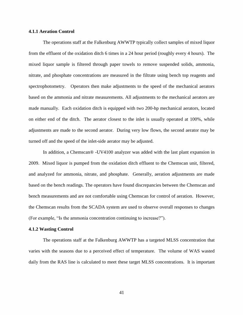
41

4.1.1 Aeration Control

The operations staff at the Falkenburg AWWTP typically collect samples of mixed liquor

from the effluent of the oxidation ditch 6 times in a 24 hour period (roughly every 4 hours). The

mixed liquor sample is filtered through paper towels to remove suspended solids, ammonia,

nitrate, and phosphate concentrations are measured in the filtrate using bench top reagents and

spectrophotometry. Operators then make adjustments to the speed of the mechanical aerators

based on the ammonia and nitrate measurements. All adjustments to the mechanical aerators are

made manually. Each oxidation ditch is equipped with two 200-hp mechanical aerators, located

on either end of the ditch. The aerator closest to the inlet is usually operated at 100%, while

adjustments are made to the second aerator. During very low flows, the second aerator may be

turned off and the speed of the inlet-side aerator may be adjusted.

In addition, a Chemscan® -UV4100 analyzer was added with the last plant expansion in

2009. Mixed liquor is pumped from the oxidation ditch effluent to the Chemscan unit, filtered,

and analyzed for ammonia, nitrate, and phosphate. Generally, aeration adjustments are made

based on the bench readings. The operators have found discrepancies between the Chemscan and

bench measurements and are not comfortable using Chemscan for control of aeration. However,

the Chemscan results from the SCADA system are used to observe overall responses to changes

(For example, “Is the ammonia concentration continuing to increase?”).

4.1.2 Wasting Control

The operations staff at the Falkenburg AWWTP has a targeted MLSS concentration that

varies with the seasons due to a perceived effect of temperature. The volume of WAS wasted

daily from the RAS line is calculated to meet these target MLSS concentrations. It is important

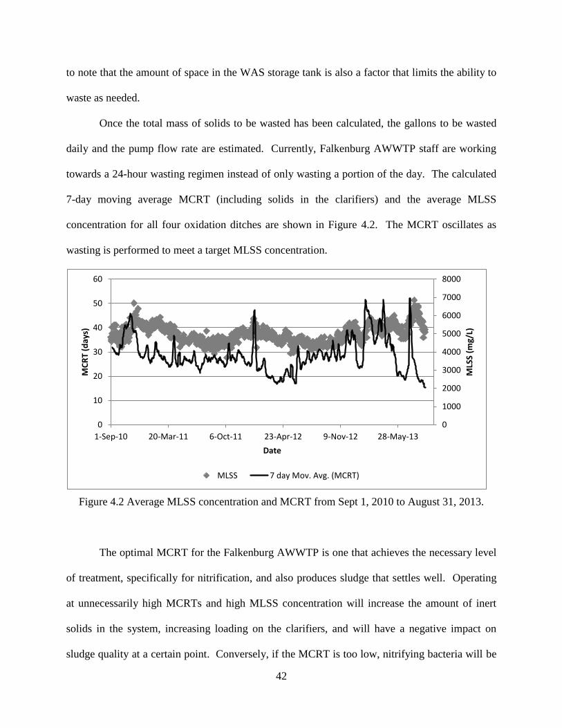
42

to note that the amount of space in the WAS storage tank is also a factor that limits the ability to

waste as needed.

Once the total mass of solids to be wasted has been calculated, the gallons to be wasted

daily and the pump flow rate are estimated. Currently, Falkenburg AWWTP staff are working

towards a 24-hour wasting regimen instead of only wasting a portion of the day. The calculated

7-day moving average MCRT (including solids in the clarifiers) and the average MLSS

concentration for all four oxidation ditches are shown in Figure 4.2. The MCRT oscillates as

wasting is performed to meet a target MLSS concentration.

Figure 4.2 Average MLSS concentration and MCRT from Sept 1, 2010 to August 31, 2013.

The optimal MCRT for the Falkenburg AWWTP is one that achieves the necessary level

of treatment, specifically for nitrification, and also produces sludge that settles well. Operating

at unnecessarily high MCRTs and high MLSS concentration will increase the amount of inert

solids in the system, increasing loading on the clarifiers, and will have a negative impact on

sludge quality at a certain point. Conversely, if the MCRT is too low, nitrifying bacteria will be

0

1000

2000

3000

4000

5000

6000

7000

8000

0

10

20

30

40

50

60

1-Sep-10 20-Mar-11 6-Oct-11 23-Apr-12 9-Nov-12 28-May-13

MLS

S (m

g/L)

MC

RT

(day

s)

Date

MLSS 7 day Mov. Avg. (MCRT)

43

washed out of the system and ammonia concentration will increase in the effluent. One concern

that was mentioned by the operating staff was not knowing when nitrifying and denitrifying

organisms are being wasted because both organisms are present in a single sludge.

4.1.3 Data Comparisons between Laboratories

Concentrations of total P, ammonia, and nitrate in the final effluent measured by the

County laboratory for reporting purposes and in filtered mixed liquor samples from the effluent

of the oxidation ditch measured by operators in the plant laboratory are shown in Figure 4.3.

Total P results were similar, while discrepancies between ammonia and nitrate values were

observed. This suggests that further nitrification is occurring after the oxidation ditch. Biofilms

located after the ditch in the deep bed media filters could further nitrify the effluent with

sufficient DO. Further research to measure DO, as well as ammonia and nitrate before and after

the filters could aid in identifying the source of the data discrepancies. Another possibility is that

the two methods used by the respective labs produce varying results.

The BioWin model outputs were compared to the County laboratory data. If the data

recorded by the operators are correct, the model predictions should be calibrated to these values.

It is recommended that a filtered sample of mixed liquor be taken to the County lab for analysis.

This may be especially important since the operators use the values obtained from their bench-

top lab to make adjustments to the mechanical aerators.

44

Figure 4.3 Concentration of total phosphorus (A), ammonia (B), and nitrate (C) measured in the

final effluent by the County lab and in filtered mixed liquor at the effluent of the oxidation ditch

measured by operators in the plant lab.

0.00

0.20

0.40

0.60

0.80

1.00

1.20

1.40

09/01/10 10/28/10 12/24/10 02/19/11 04/17/11 06/13/11 08/09/11

Ph

osp

ho

rus

(mg/

L)

PO4 Plant lab Total P County Lab

0.00

0.50

1.00

1.50

2.00

2.50

1-Sep-10 28-Oct-10 24-Dec-10 19-Feb-11 17-Apr-11 13-Jun-11 9-Aug-11

Am

mo

nia

(m

g/L)

NH3 Plant lab NH3 County Lab

0.00

0.50

1.00

1.50

2.00

2.50

3.00

3.50

09/01/10 10/28/10 12/24/10 02/19/11 04/17/11 06/13/11 08/09/11

Nit

rate

(m

g/L)

NO3 Plant lab NO3 County Lab

B

C

A

45

4.2 BioWin Calibration and Validation

A calibration and validation were performed for the Falkenburg BioWin model. This

required supplemental sampling to be carried out for wastewater characterization to obtain values

for COD and VSS. These values were used along with historical plant data to determine influent

wastewater fractions for the model. Several kinetic parameters were adjusted during the

calibration and goodness of fit analyses were used to select the best parameter arrangement.

Finally, the model was validated using a dataset from a time period other than that used during

calibration.

4.2.1 Wastewater Characterization

The results of the COD analyses on influent and effluent samples are shown in Figure

4.4. All influent samples were 24-hour composites and secondary effluent samples were grab

samples. It is important to note that the effluent grab sample was collected from the secondary

clarifier effluent before the media filters.

Figure 4.4 COD results from wastewater characterization. For influent n=5, for effluent n=2.

557

364

160

20

0

100

200

300

400

500

600

700

CO

D (

mg/

L) Unfiltered Influent COD

Filtered Influent COD

Flocculated-Filtered Influent COD

Effluent COD

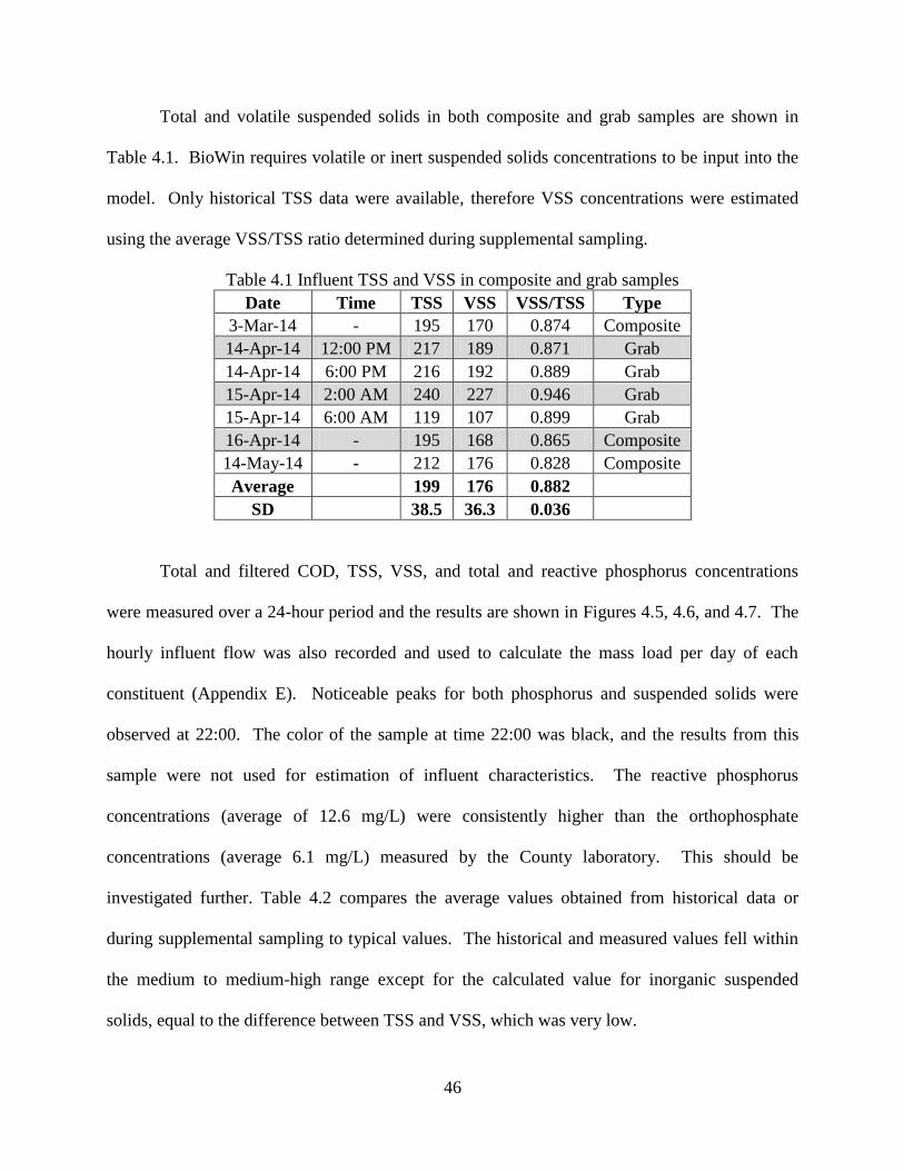
46

Total and volatile suspended solids in both composite and grab samples are shown in

Table 4.1. BioWin requires volatile or inert suspended solids concentrations to be input into the

model. Only historical TSS data were available, therefore VSS concentrations were estimated

using the average VSS/TSS ratio determined during supplemental sampling.

Table 4.1 Influent TSS and VSS in composite and grab samples

Date Time TSS VSS VSS/TSS Type

3-Mar-14 - 195 170 0.874 Composite

14-Apr-14 12:00 PM 217 189 0.871 Grab

14-Apr-14 6:00 PM 216 192 0.889 Grab

15-Apr-14 2:00 AM 240 227 0.946 Grab

15-Apr-14 6:00 AM 119 107 0.899 Grab

16-Apr-14 - 195 168 0.865 Composite

14-May-14 - 212 176 0.828 Composite

Average

199 176 0.882

SD

38.5 36.3 0.036

Total and filtered COD, TSS, VSS, and total and reactive phosphorus concentrations

were measured over a 24-hour period and the results are shown in Figures 4.5, 4.6, and 4.7. The

hourly influent flow was also recorded and used to calculate the mass load per day of each

constituent (Appendix E). Noticeable peaks for both phosphorus and suspended solids were

observed at 22:00. The color of the sample at time 22:00 was black, and the results from this

sample were not used for estimation of influent characteristics. The reactive phosphorus

concentrations (average of 12.6 mg/L) were consistently higher than the orthophosphate

concentrations (average 6.1 mg/L) measured by the County laboratory. This should be

investigated further. Table 4.2 compares the average values obtained from historical data or

during supplemental sampling to typical values. The historical and measured values fell within

the medium to medium-high range except for the calculated value for inorganic suspended

solids, equal to the difference between TSS and VSS, which was very low.

47

Figure 4.5 Total and filtered influent COD.

Figure 4.6 Total and volatile influent suspended solids.

Figure 4.7 Total and reactive influent phosphorus.

0

100

200

300

400

500

600

700

800

8:00 10:00 12:00 14:00 16:00 18:00 20:00 22:00 0:00 2:00 4:00

CO

D (

mg/

L)

Time

Total COD Filtered COD

0

50

100

150

200

250

300

350

8:00 10:00 12:00 14:00 16:00 18:00 20:00 22:00 0:00 2:00 4:00

Susp

en

de

d S

olid

s m

g/L

Time

TSS VSS

0.0

5.0

10.0

15.0

20.0

25.0

30.0

35.0

40.0

8:00 10:00 12:00 14:00 16:00 18:00 20:00 22:00 0:00 2:00 4:00

Ph

osp

ho

rus

mg/

L

Time

Total P Reactive P

48

Table 4.2 Comparison of literature values to average values of influent parameters from

historical data and supplemental sampling

Parameter

Range in mg/L (Metcalf & Eddy, 2003) Falkenburg

Average

Data

(mg/L)

Data Source Strength Low Strength

Medium Strength

High Strength

COD 250 430 800 557 Measured in USF lab Medium-

High

BOD 110 190 350 290 Historical County data Medium-

High

TSS 120 210 400 192 / 205 Historical County data /

Measured in USF lab Medium

VSS 95 160 315 169 / 181 Measured in USF lab/

Estimated from historical

TSS data Medium

ISS 25 50 85 24 Calculated from TSS &

VSS measured in USF

lab Low

TKN 20 40 70 51.2 Historical County data Medium-

High

TP 4 7 12 6.1 Historical County data Medium

The calculated values from BioWin Influent Specifier Excel worksheet are given in Table

4.3. Some values were calculated using the results from the COD analyses (Figure 4.4), while

others such as the unbiodegradable particulate fraction had to be estimated.

Table 4.3 BioWin wastewater fractions

Fraction Symbol Units BioWin

Default Value

Calculated

Value

Readily biodegradable COD Fbs g COD/g CODtotal 0.16 0.254

Acetate Fac g COD/g rbCOD 0.15 0.141

Non-colloidal slowly

biodegradable COD

Fxsp g COD/ g slowly

biodegradable COD 0.75 0.400

Soluble unbiodegradable COD Fus g COD/g CODtotal 0.05 0.033

Particulate unbiodegradable COD Fup g COD/g CODtotal 0.13 0.110

Ammonia Fna g NH3-N/g TKN 0.66 0.743

Particulate organic N Fnox g N/g organic N 0.5 0.500

Soluble unbiodegradable TKN Fnus g N/g TKN 0.02 0.000

N:COD ratio for unbiodegradable

particulate COD

FupN g N/g COD 0.35 0.35

Phosphate Fpo4 g PO4-P/ g TP 0.5 0.638

P:COD ratio for unbiodegradable

particulate COD

FupP g P/g COD 0.011 0.011

49

4.2.2 Goodness of Fit

The average SAR results are given in Table 4.4. A lower number indicated a better fit of

modeled to observed data. Although Simulations 8 and 9 resulted in lower SAR, Simulation 5

parameters were selected as the best fit. The values in Simulation 5 for the heterotrophic and

aerobic denit. DO half saturation constants were close to the value of 0.25 mgO2/L

recommended by EnviroSim to model SND in an oxidation ditch. It was not known if a value of

0.5 mg O2/L was a reasonable adjustment, and the improvement in results between Simulation 5

and 8 or 9 were less than those observed with the change seen between Simulations 3 or 4 and

Simulation 5. The final calibrated kinetic parameters are shown in Table 4.5.

Table 4.4 Average sum of absolute residuals of effluent N concentrations with varying kinetic

parameters

Simulation Effluent NH3-N

(mg/L)

Effluent TKN

(mg/L)

Effluent NO3

(mg/L)

Effluent NO2

(mg/L)

1* 1.01 1.37 1.90 0.865

2 0.781 1.14 1.84 0.833

3 0.665 0.999 1.23 0.336

4 0.784 1.12 1.02 0.397

5 0.437 0.778 0.908 0.291

6 0.567 0.905 0.884 0.355

7 0.614 0.934 1.09 0.284

8 0.436 0.769 0.789 0.204

9 0.368 0.680 0.807 0.193

*BioWin default kinetic parameter values

50

Table 4.5 BioWin kinetic parameters

Parameter Default Value Calibrated Value AOB Maximum Specific Growth Rate

0.9 0.9

NOB Maximum Specific Growth Rate 0.7 0.7

OHOs Maximum Specific Growth Rate 3.2 3.2

Heterotrophic DO half saturation constant 0.05 0.3

Aerobic denitrification DO half saturation constant 0.05 0.3

Ammonia oxidizer DO half saturation constant 0.25 0.15

Nitrite oxidizer DO half saturation constant 0.5 0.5

Anaerobic ammonia oxidizer DO half saturation constant 0.01 0.01

Anoxic NO3-N half saturation constant 0.1 0.1

Anoxic NO2-N half saturation constant 0.01 0.05

NH3-N nutrient half saturation constant 1.00E-04 1.00E-04

Charts were prepared in the BioWin model to plot modeled values against data observed

at the Falkenburg AWWTP from September 1, 2010 to August 31, 2014. The modeled MLSS

concentration in the calibrated model was charted against the observed MLSS (Figure 4.8).

These concentrations resulted from a constant average wasting rate of 0.234 mgd. Changing the

daily WAS flow to more accurately reflect plant wasting could produce a better fit of modeled to

observed data.

Figure 4.8 Observed (green squares) and modeled (pink line) MLSS concentration.

DATE

9/1/20117/1/20115/1/20113/1/20111/1/201111/1/20109/1/2010

MLS

S (m

g/L)

7,000

6,500

6,000

5,500

5,000

4,500

4,000

3,500

3,000

2,500

2,000

1,500

1,000

500

0

ML

SS

(m

g/L

)

51

A poor fit was observed between modeled and observed MLVSS concentrations (Figure

4.9). The model-predicted MLVSS is usually adjusted by changing the influent unbiodegradable

particulate COD fraction. However, it was not known if the discrepancy in MLVSS was solely

attributed to model input or if addition of alum played a role. Metal hydroxides, such as those

formed during alum addition, are oxidized during VSS analysis in the muffle furnace, which will

result in a falsely high MLVSS concentration (Jeyanayagam and Husband, 2009). Adjustments

to influent COD fractions could be made once it is determined if alum is contributing to the VSS

concentration.

Figure 4.9 Observed (blue squares) and modeled (pink line) MLVSS concentration.

Spikes in effluent nitrogen species were observed several times during the year-long

simulation (Figure 4.10). These spikes correspond with the influent loading of TKN (Figure

4.11). The model is sensitive to N loading at higher flow or higher influent TKN concentration.

In the WWTP, operators make changes to mechanical aerator speed in response to oxidation

ditch ammonia concentration. The model maintained a constant DO set point in the mechanical

aerator reactors. Fine-tuning the model aeration settings to better reflect the aeration practices of

DATE

8/1/20117/1/20116/1/20115/1/20114/1/20113/1/20112/1/20111/1/201112/1/201011/1/201010/1/20109/1/2010

ML

VS

S (m

gV

SS

/L)

7,000

6,800

6,600

6,400

6,200

6,000

5,800

5,600

5,400

5,200

5,000

4,800

4,600

4,400

4,200

4,000

3,800

3,600

3,400

3,200

3,000

2,800

2,600

2,400

2,200

2,000

1,800

1,600

1,400

1,200

1,000

800

600

400

200

0

ML

VS

S (

mg/L

)

52

the WWTP could reduce the modeled effluent spikes, and produce improved goodness-of-fit of

modeled to observed parameters.

Figure 4.10 Observed (red squares) and modeled (blue line) effluent TKN concentration.

Figure 4.11 Influent TKN mass load.

4.2.3 Sensitivity Analysis

The results of sensitivity analysis show that altering kinetic parameters affects the

resultant effluent concentrations differently (Table 4.6). AOB maximum specific growth rate is

very influential for effluent ammonia concentrations. The maximum specific growth rate for

DATE

8/15/20117/16/20116/16/20115/17/20114/17/20113/18/20112/16/20111/17/201112/18/201011/18/201010/19/20109/19/2010

Eff

lue

nt

TK

N (

mg

N/L

)

3

2

1

0

DATE

8/15/20117/16/20116/16/20115/17/20114/17/20113/18/20112/16/20111/17/201112/18/201011/18/201010/19/20109/19/2010

INF

LU

EN

T T

KN

MA

SS

RA

TE

(lb

N/d

)

7,000

6,500

6,000

5,500

5,000

4,500

4,000

3,500

3,000

2,500

2,000

1,500

1,000

500

0

Eff

luen

t T

KN

(m

g N

/L)

Infl

uen

t T

KN

Mas

s R

ate

(lbN

/day

)

53

nitrite oxidizing bacteria does not influence the effluent ammonia concentration, but is very

influential on effluent nitrite and nitrate concentration. The combined heterotrophic/aerobic

denit DO half saturation constant is most influential on effluent nitrate concentration. This is

expected because this constant switches on the activity of anoxic OHOs under low DO

conditions. By increasing this parameter, the anoxic OHO activity is turned on at a higher

concentration of DO. The ammonia oxidizer DO half saturation constant was only slightly

influential on the ammonia concentration, while the anoxic NO2 half saturation constant mostly

influenced the effluent nitrate concentration. The anoxic NO2 half saturation constant switches

off anoxic growth process at low nitrite concentrations.

Table 4.6 Sensitivity analysis for kinetic parameters

AOB max spec

growth rate

NOB max spec

growth rate

Heterotrophic/

Aerobic denit

DO Half Sat

Ammonia

Oxidizer DO

Half Sat

Anoxic NO2

Half Sat

Δx 0.1 0.1 0.1 0.1 0.01

Ammonia 2.45 0 0.273 0.409 0

Nitrate 1.14 2.43 1.21 0.237 0.71

Nitrite 0.474 1.84 0.474 0 0.263

4.2.4 Validation

Data from September 1, 2011 to August 31, 2012 were entered into the calibrated

BioWin model and the model was simulated for a one year period. The modeled effluent

concentrations were compared to observed effluent concentrations measured by the County

laboratory for the same period. Results of the goodness of fit comparison using the average sum

of absolute residuals are shown in Table 4.7. The goodness of fit was comparable to the fit

obtained during the calibration except for nitrate. Nitrate concentrations modeled during the

validation were relatively high. The concentration of effluent nitrate is important and the

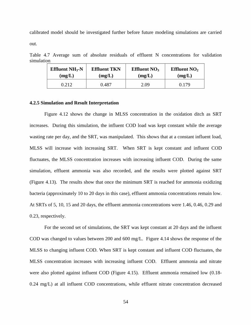
54

calibrated model should be investigated further before future modeling simulations are carried

out.

Table 4.7 Average sum of absolute residuals of effluent N concentrations for validation

simulation

Effluent NH3-N

(mg/L)

Effluent TKN

(mg/L)

Effluent NO3

(mg/L)

Effluent NO2

(mg/L)

0.212 0.487 2.09 0.179

4.2.5 Simulation and Result Interpretation

Figure 4.12 shows the change in MLSS concentration in the oxidation ditch as SRT

increases. During this simulation, the influent COD load was kept constant while the average

wasting rate per day, and the SRT, was manipulated. This shows that at a constant influent load,

MLSS will increase with increasing SRT. When SRT is kept constant and influent COD

fluctuates, the MLSS concentration increases with increasing influent COD. During the same

simulation, effluent ammonia was also recorded, and the results were plotted against SRT

(Figure 4.13). The results show that once the minimum SRT is reached for ammonia oxidizing

bacteria (approximately 10 to 20 days in this case), effluent ammonia concentrations remain low.

At SRTs of 5, 10, 15 and 20 days, the effluent ammonia concentrations were 1.46, 0.46, 0.29 and

0.23, respectively.

For the second set of simulations, the SRT was kept constant at 20 days and the influent

COD was changed to values between 200 and 600 mg/L. Figure 4.14 shows the response of the

MLSS to changing influent COD. When SRT is kept constant and influent COD fluctuates, the

MLSS concentration increases with increasing influent COD. Effluent ammonia and nitrate

were also plotted against influent COD (Figure 4.15). Effluent ammonia remained low (0.18-

0.24 mg/L) at all influent COD concentrations, while effluent nitrate concentration decreased

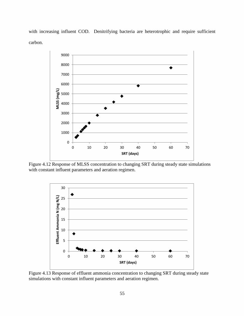
55

with increasing influent COD. Denitrifying bacteria are heterotrophic and require sufficient

carbon.

Figure 4.12 Response of MLSS concentration to changing SRT during steady state simulations

with constant influent parameters and aeration regimen.

Figure 4.13 Response of effluent ammonia concentration to changing SRT during steady state

simulations with constant influent parameters and aeration regimen.

0

1000

2000

3000

4000

5000

6000

7000

8000

9000

0 10 20 30 40 50 60 70

MLS

S (m

g/L)

SRT (days)

0

5

10

15

20

25

30

0 10 20 30 40 50 60 70

Effl

ue

nt

Am

mo

nia

N (

mg

N/L

)

SRT (days)

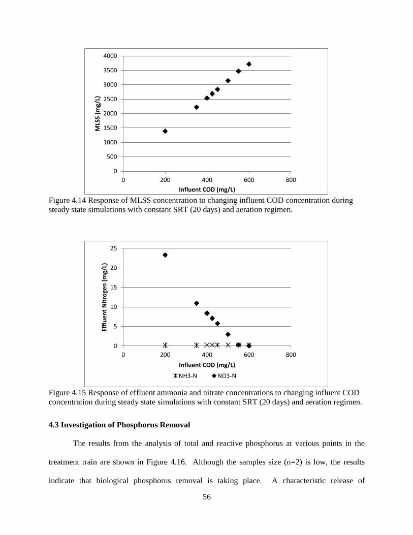
56

Figure 4.14 Response of MLSS concentration to changing influent COD concentration during

steady state simulations with constant SRT (20 days) and aeration regimen.

Figure 4.15 Response of effluent ammonia and nitrate concentrations to changing influent COD

concentration during steady state simulations with constant SRT (20 days) and aeration regimen.

4.3 Investigation of Phosphorus Removal

The results from the analysis of total and reactive phosphorus at various points in the

treatment train are shown in Figure 4.16. Although the samples size (n=2) is low, the results

indicate that biological phosphorus removal is taking place. A characteristic release of

0

500

1000

1500

2000

2500

3000

3500

4000

0 200 400 600 800

MLS

S (m

g/L)

Influent COD (mg/L)

0

5

10

15

20

25

0 200 400 600 800

Effl

ue

nt

Nit

roge

n (

mg/

L)

Influent COD (mg/L)

NH3-N NO3-N

57

phosphorus is observed in the unaerated selector, followed by very low phosphorus in the

effluent of the aerated reactor. The average release of phosphate in the selector was 32 mg/L,

and the total amount of phosphate removed was 45 mg/L. Similar phosphate release and uptake

were reported by Henze (2008) with a phosphate release of 45 mg/L, uptake of 57 mg/L, and

total removal of 12 mg/L. It is not possible to assume the removal of P in the ditch is fully

attributed to EBPR since aluminum sulfate (alum) is also added for chemical phosphorus

removal. Alum is dosed at a constant rate (~260 gpd) into a splitter box after the oxidation

ditches and before the secondary clarifiers. Jar testing to determine the optimum dose of alum

was discussed with plant staff, but this was later determined to be unfeasible due to the presence

of alum in the RAS and mixed liquor. Flow-pacing of alum and slowly decreasing alum dosing

while observing the effect on effluent total phosphorus concentration are suggested. This will

reduce chemical costs, sludge production, and possible impacts of alum on the biological

process.

Figure 4.16 Reactive phosphorus profile from grab samples taken throughout the treatment

process.

0

10

20

30

40

50

60

Ph

osp

ho

rus

(mg/

L)

Total Phosphorus Reactive Phosphorus

Influent Selector Oxidation Ditch

Effluent Secondary Effluent

58

CHAPTER 5: CONCLUSIONS AND RECOMMENDATIONS

The Operations Staff at the Falkenburg AWWTP consistently meet and exceed NPDES

permit limits. In addition to meeting permit, the goal of the operator is to also reduce costs and

energy usage associated with plant operation. These savings will reduce emissions of

greenhouse gases and costs to County ratepayers. There are three areas where improvements

could be made to improve efficiency of operation: 1) alum addition for phosphorus removal 2)

wasting based on MCRT and 3) online aeration control based on ammonia concentration.

Activated sludge modeling enables the user to observe the virtual effect of changes in operation

and influent loading relatively quickly and without risk of permit violation. A BioWin model

was created for the Falkenburg AWWTP, and several simulations were run to observe

relationships between MLSS, MCRT, and influent loads. Finally, data compilation and

reconciliation conducted during this study highlighted many good practices in plant operation

and monitoring, with only a few gaps for future improvement.

The addition of alum for phosphorus removal at the Falkenburg AWWTP should be

optimized to ensure that NPDES permits are met without overdosing. In addition to reducing

costs and chemical usage, improvements in sludge dewatering may result from optimization of

alum addition. A brief investigation of phosphorus throughout the treatment train showed a

release of phosphorus in the anaerobic selector characteristic of enhanced biological phosphorus

removal. The Operations Staff at the Falkenburg AWWTP is planning to reduce the amount of

alum that is added for chemical phosphorus removal by flow-pacing and observing the effects of

an overall decrease in dose. Because alum addition also improves settling in the clarifiers, a

59

reduction in alum addition may increase secondary effluent turbidity if sludge quality is poor and

further necessitate finding the MCRT where sludge quality is best.

The time that bacteria remain in the system, the SRT or MCRT, is one of the most

important factors affecting plant performance. The optimal MCRT for the Falkenburg AWWTP

should be found and wasting practices should be changed to maintain this target MCRT.

Currently, wasting is controlled by keeping the constant MLSS method, while disregarding

fluctuations in MCRT. The optimal MCRT for the Falkenburg AWWTP is one that achieves the

necessary level of treatment, specifically for nitrification, and also produces sludge that settles

well. Operating at unnecessarily high MCRTs and high MLSS concentration will increase the

amount of inert solids in the system, increasing loading on the clarifiers, and can have a negative

impact on sludge quality. For nitrification, it is important to know the MCRT of solids that are

under aeration. Currently, the MCRT calculation at the Falkenburg AWWTP incorporates the

mass of solids in the clarifiers as well. It is recommended that both the MCRT of the total

system and the aerobic MCRT be calculated to ensure that the minimum sludge age for

nitrification is being met. One challenge in calculating sludge age, as well as SVI, is accurately

measuring the MLSS concentration. MLSS concentrations can fluctuate over the course of a day,

and collecting and analyzing one grab sample per day may not adequately represent the MLSS

concentration. A composite sample of MLSS will give a more accurate estimate of the average

MLSS concentration. Another option is a MLSS analyzer that can measure concentrations

quickly and more frequently and can be coupled with the SCADA system.

Implementing aeration control using online analyzers is increasingly being used at

AWWTPs. The use of online analyzers allows for more frequent monitoring of aeration basin

conditions and automatic adjustment based on pre-defined parameters. The Falkenburg

60

AWWTP has ChemScan units that monitor ammonia, phosphate, and nitrate. Automatic control

of mechanical aerators should be reevaluated as a process control option for nitrification and

denitrification. The online analyzers will be able to respond more quickly to changes in influent

ammonia loads. Although aeration is critical, it is important to remember the role of MCRT in

nitrification as well. A minimum MCRT must be met to allow nitrifiers to grow in the system.

One objective of this study was to construct and calibrate a BioWin model of the

Falkenburg AWWTP. The BioWin model was able to achieve simultaneous nitrification and

denitrification in the modeled oxidation ditch by adjusting several half saturation constants. The

model was calibrated for nitrification and denitrification. If phosphorus removal is to be

investigated, the model should be reevaluated. The model was found to be sensitive to changes

in the maximum specific growth rates of ammonia and nitrite oxidizing bacteria. These

parameters should be measured experimentally for future model calibration. A limited number of

simulations were run with the model. Steady state simulations were run with the model to

observe the effect of variable and constant SRT (or MCRT) and changing influent loads. In each

simulation only one variable was manipulated. While this is not reflective of normal plant

operation, it allows the effect of each variable change to be observed. Plotting effluent ammonia

concentration at varying SRT shows that SRT has little effect at decreasing ammonia

concentration after the minimum MCRT needed for nitrification is reached. As SRT increases,

the MLSS increases due to the buildup of inert solids. At constant SRT, MLSS varies with

influent COD concentration, because bacteria grow as food becomes available. Mixed liquor

suspended solids is a response variable and should not be used as a control variable.

Comparisons of oxidation ditch effluent collected and analyzed by plant operators and

final effluent samples analyzed by the Hillsborough County certified laboratory showed

61

relatively good agreement, especially for phosphorus. Small differences in ammonia and nitrate

were observed, which may be due to further biological activity after the oxidation ditch.

Ammonia, nitrate, and DO should be measured at points between the oxidation ditch and final

effluent to further investigate these discrepancies. BioWin modeling requires additional inputs,

such as VSS and fractions of COD, which are not currently measured at the Falkenburg

AWWTP. Periodically monitoring these parameters will aid in future modeling projects. It was

also not possible to fully assess the operation of the clarifiers and sludge quality, because no data

were available on the amount of suspended solids leaving in the secondary clarifier effluent. A

simple turbidity test with secondary clarifier effluent will give the operators more information

about the ability of the sludge to flocculate and settle in the clarifiers. This will be especially

important when assessing the effect of MCRT control on sludge quality.

62

REFERENCES

Abusam, A. (2001) “Development of a benchmarking methodology for evaluating oxidation

ditch control strategies.” Ph.D. Thesis, Wageningen University, The Netherlands

APHA, AWWA, WEF (2012). “Standard Methods for the Examination of Water and

Wastewater” 23rd

edition, American Public Health Association, Washington D.C.

Ardern, E. and Lockett, W. (1914) “Experiments on the oxidation of sewage without the aid of

filters.” J. of the Society of Chem. Industry. 33 (10) 523-539

Arthur, R. (1983) “Process control strategies.” Procedures and practices in activated sludge

process control, Arthur, R, ed. Butterworth Publishers, Boston, MA, 25-44

Austin, J., McLellon, W., and Dyer, J. (1970) “Training the environmental technician.”

A.J.P.H. 60 (12) 2314-2320

Barnard, J. (1975) “Biological nutrient removal without the addition of chemicals.” Water

Research 9 (5-6) 485-490

Barnard, J., Steichen, M., and deBarbadillo C. (2004) “Interaction between aerator type and

simultaneous nitrification and denitrification.” Proceedings of the 77th

Annual Water

Environment Federation Technical Exposition and Conference, New Orleans, LA

Oct 2-6, 359-377

Bond, P., Keller, J., and Blackall, C. (1999) “Bio-P and non-bio-P bacteria identification by a

novel microbial approach.” Wat. Sci. and Tech. 39(6) 13-20

Bowker, R, and Stensel, H. D. (1990) “Phosphorus Removal from Wastewater.” Noyes Data

Corporation, New Jersey

Bratby, J., and Fevig, S. (2012) “Am I sampling too little or too much?: A template guides plant

operators on the right areas and ways to sample for process control.” Water Environ. and

Tech.

Bye, C. and Dold, P. (1998) “Sludge volume index settleability measures: effect of solids

characteristics and test parameters.” Wat. Environ. Res. 70, 87-93

Daigger, G., Waltrip, D., Romm, E., and Morales, L. (1988) “Enhanced secondary treatment

incorporating biological nutrient removal.” J. Wat. Pol. Cont. Fed. 60(10) 1833-1842

63

Daigger, G., and Littleton, H. (2000) “Characterization of simultaneous nutrient removal in

staged, closed-loop bioreactors” Wat. Environ. Res. 72(3) 330-339

Daigger, G., Adams, C., and Steller H. (2007) “Diffusion of oxygen through activated sludge

flocs: Experimental measurement, modeling, and implications for simultaneous

nitrification and denitrification.” Wat. Environ. Res., 79, 375-387

Daigger, G. and Littleton, H. (2014) “Simultaneous biological nutrient removal: a state-of-the-art

review.” Wat. Environ. Res. 86(3)245-257

Envirosim (n.d.) “Changes to three default kinetic parameters in BioWin 3.0.1”

http://www.envirosim.com/downloads/BW301SND.pdf

Dey, A. (2010) “Modeling simultaneous nitrification-denitrification process in an activated

sludge continuous flow stirred-tank reactor: System optimization and sensitivity

analysis.” Environ. Eng. Sci. 27(9) 757-765

Dold, P., Ekama, G., and Marais, G. (1980) “The Activated Sludge Process 1. A general model

for the activated sludge process.” Progress in Wat. Tech. 12 (6) 47-77

Ekama, G., and Wentzel, M. (1999) “Difficulties and developments in biological nutrient

removal technology and modelling.” Wat. Sci. and Tech. 39(6) 1-11

Ekama, G. (2009) “Using bioprocess stoichiometry to build a plant-wide mass balance based

steady-state WWTP model.” Water Research 43(8) 2101-2120

EPA (2002) “Federal water pollution control act: As amended through P.L. 107-303,

November 27, 2002.” http://www.epw.senate.gov/water.pdf

Falk, M., Neethling, JB., and Reardon, D., (2011) “Striking the balance between nutrient

removal in wastewater treatment and sustainability.” WERF and IWA Publishing

Gori, R., Giaccherini, F., Jiang, L., Sobhani, R., and Rosso, D. (2013) “Role of primary

sedimentation on plant-wide energy recovery and carbon footprint.” Wat. Sci. and Tech.

68(4) 870-878

Grady, L., Daigger, G., and Lim, H. (1999) “Biological Wastewater Treatment.” 2nd

Edition.

Marcel Dekker, Inc. New York, NY.

Hauduc, H., Gillot, S., Rieger, L., Ohtsuki, T., Shaw, A., Takács, I., and Winkler, S. (2009)

“Activated sludge modelling in practice: an international survey.” Wat. Sci. and Tech.

60(8) 1943-1951

64

Henze, M., Gujer, W., Mino, T., and van Loosdrecht, M. (2000) “Activated sludge models

ASM1, ASM2, ASM2d, and ASM3. IWA task group on mathematical modelling for

design and operation of biological wastewater treatment. No 9. IWA scientific and

technical report.

Henze, M., Harremoës, P., la Cour Jansen, J., and Arvin, E. (2002) “Wastewater Treatment:

Biological and chemical processes.” 3rd

Edition, Springer ISBN 3-540-42228-5

Henze, M., van Loosdrecht, M. C. M., Ekama, G. A., and Brdjanovic, P. (2008) “Biological

wastewater treatment: Principles, Modelling, and Design. IWA Publishing

Hu, Z., Wentzel, M., and Ekama, G. (2002) “Anoxic growth of phosphate accumulating

organisms (PAOs) in biological nutrient removal activated sludge systems.” Water

Research. 39 (19) 4927-4937

Hulsbeek, J., Roeleveld, P., and van Loosdrecht, M. (2002) “A practical protocol for dynamic

modelling of activated sludge systems.” Wat. Sci. and Tech. 45(6) 127-136

Ingildsen,P., Rosen, C., Gernaey, K., Nielsen, M., Guildal, T., and Jacobsen, B. (2006)

“Modelling and control strategy testing of biological and chemical phosphorus removal

at Avedore WWTP.” Wat. Sci. and Tech. 53(4-5) 105-113

Insel, G. (2007) “Effects of design and aeration control parameters on simultaneous nitrification

and denitrification (SNdN) performance for activated sludge process.” Env. Eng. Sci. 24

(5) 675-686

Jenicek, P., Kutil, J., Benes, O., Todt, V., Zabranska, J., and Dohanyos, M. (2013) “Energy self-

sufficient sewage wastewater treatment plants: Is optimized anaerobic sludge digestion

the key?” Wat. Sci. and Tech. 68(8) 1739-1744

Jenkins, D., Richard, M., and Daigger G. (1993) “Manual on the causes and control of activated

sludge bulking and foaming.” Lewis Publishers. Chelsea, Michigan

Jeyanayagam, S and Husband, J. (2009) “Chain reaction: How chemical phosphorus removal

really works.” Water Environ. and Tech. 21 (4)

Jimenez, J., Dursun, D., Dold, P., Bratby, J., Keller, J., and Parker, D. (2010) “Simultaneous

nitrification-denitrification to meet low effluent nitrogen limits: Modeling, Performance,

and Reliability.” Proceedings of the 83th

Annual Water Environment Federation

Technical Exposition and Conference, New Orleans, LA, Oct 2-6, 2010, 2404-

2421

Jimenez, J., Bott, C., Regmi, P., and Riger, L. (2013) “Process control strategies for

simultaneous nitrogen removal systems.” WEF/IWA Nutrient Removal and Recovery

Conference, July 28-31, 2013, Vancouver, British Columbia

65

Ju, L., Huang, L., and Trivedi, H. (2007) “Simultaneous nitrification, denitrification and

phosphorus removal in single-tank low-dissoloved-oxygen systems under cyclic

aeration.” Wat. Environ. Res. 79(8) 912-920

Langergraber, G., Rieger, L., Winkler, S., Alex, J., Wiese, J., Owerdieck, C., Ahnert, M.,

Simon, J., and Maurer M. (2004) “A guideline for simulation studies of wastewater

treatment plants.” Wat. Sci. and Tech. 50(7)131-138

Littleton, H., Daigger, G., and Strom, P. (2007) “Application of computational fluid dynamics

to closed-loop bioreactors: II. Simulation of biological phosphorus removal using

computational fluid dynamics.” Wat. Environ. Res. 79, 613-624

Liwarska-Bizukojc, E., and Biernacki, R. (2010) “Identification of the most sensitive parameters

in the activated sludge model implemented in BioWin software.” Bioresource

Technology. 101, 7278-7285

Ludzack, F. and Ettinger, M. (1962) “Controlling operation to minimize activated sludge effluent

nitrogen.” J. Wat. Poll. Control Fed. 34(9) 920-931

Mamais, D., Jenkins, D., and Pitt, P. (1993) “A rapid physical-chemical method for the

determination of readily biodegradable soluble COD in municipal wastewater.” Water

Research 27(1) 195-197

Mandt, M. and Bell, B. (1982) “Oxidation ditches in wastewater treatment.” Ann Arbor Science,

Ann Arbor, Michigan

Melcer, H., Dold, P., Jones, R., Bye, C., Takacs, I., Stensel, D., Wilson, W., Sun, P., and Bury, S.

(2003) “Methods for wastewater characterization in activated sludge modeling”. WERF

Metcalf & Eddy, Inc. (2003) “Wastewater engineering: treatment, disposal, and reuse.”

McGraw-Hill, New York, New York.

Mikola, A., Rautianinen, J., and Vahala, R. (2009) “Secondary clarifier conditions conducting to

secondary phosphorus release in a BNR plant.” Wat. Sci. and Tech. 60(9) 2413-2418

Mino, T., van Loosdrecht, M.C.M., and Heinjnen, J. (1998) “Microbiology and biochemistry of

the enhanced biological phosphate removal process.” Water Research 32(11) 3193-3207

Mo, W., and Zhang, Q. (2012) “Can municipal wastewater treatment systems be carbon

neutral?” J. of Environmental Management 112, 360-367

Moussa, M., Hooijmans, C., Lubberding, H., Gijzen, H., and van Loosdrecht, M. (2005)

“Modelling nitrification, heterotrophic growth and predation in activated sludge.” Water

Research 39, 5080-5098

66

Münch, E., Lant, P., and Keller, J. (1996) “Simultaneous nitrification and denitrification in

bench-scale sequencing batch reactors.” Water Research 30 (2) 277-284

Myers, M., Myers, L., and Okey, R. (2006) “The use of oxidation-reduction potential as a means

of controlling effluent ammonia concentration in an extended aeration activated sludge

system.” Proceedings of the 79th

Annual Water Environment Federation Technical

Exposition and Conference, Dallas, TX

Oehmen, A., Lemos, P., Carvalho, G., Yuan, Z., Keller, J., Blackall, L., and Reis, M. (2007)

“Advances in enhanced biological phosphorus removal: From micro to macro scale.”

Water Research 41(11) 2271-2300

Olsson, G., and Newell, B. (1999) Wastewater Treatment Systems: Modelling, Diagnosis and

Control, IWA Publishing, London

OWP (2006) “Advanced waste treatment: A field study training program.” 5th

Edition.

OWP (2008) “Operation of wastewater treatment plants, Volume 1.” 7th

Edition.

Pagilla, K., Czerwionka, K., Urgun-Demirtas, M., and Makinai, J. (2008) “Nitrogen speciation in

wastewater treatment plant influents and effluents-the US and Polish case studies.” Wat.

Sci and Tech. 57(10) 1511-1517

Pochana, K. and Keller, J. (1999) “Study of factors affecting simultaneous nitrification and

denitrification (SND).” Wat. Sci. and Tech. 39(6) 61-68

Puig, S., van Loosdrecht, M., Colprim, J., and Meijer, S. (2008) “ Data evaluation of full-scale

wastewater treatment plants by mass balance.” Water Research 42, 4645-4655

Rieger, L., Gillot, S., Langergraber, G., Takayuki, O., Shaw, A., Takács, I., and Winkler, S.

(2012) “Guidelines for using activated sludge models.” IWA Publishing

Rieger, L., Jones, R., Dold, P., and Bott, C. (2014) “Ammonia-based feedforward and feedback

aeration control in activated sludge processes.” Wat. Environ. Res. 86(1) 63-73

Rittmann, B., and Langeland, E. (1985) “Simultaneous denitrification with nitrification in single-

channel oxidation ditches.” J. Wat. Pol. Cont. Fed. 57(4) 300-308

Schwarzenbeck, N., Bomball, E., and Pfeiffer, W. (2008) “Can a wastewater treatment plant be a

powerplant?: A case study.” Wat. Sci. and Tech. 57(10) 1555-1561

Stenstrom, M. and Poduska, R. (1980) “The effect of dissolved oxygen concentration on

nitrification.” Water Research 14(6) 643-649

Stevens, G., Barnard, J., and Rabinowitz, B. (1999) “Optimizing biological nutrient removal in

anoxic zones.” Wat. Sci. and Tech. 39(6) 113-118

67

van Niekerk, A., Jenkins, D., and Richard, M. (1989) “A mathematical model of the carbon-

limited growth of filamentous and floc-forming organisms in low F/M bulking.” J. Wat.

Pol. Cont. Fed. 60, 100-106

Vanrolleghem, P., Insel, G., Petersen, B., Sin, G., De Pauw, D., Nopens, I., Dovermann, H.,

Weijers, S., and Gernaey, K. (2003) Proceedings of the 76th

Annual Water Environment

Federation Technical Exposition and Conference, Los Angeles, California

Oct 11-15, 1996

Wahlberg, E., Crowley, J., Bower, J., Bittner, M., and Margolis, Z. (1996) “Why the activated

sludge process is so hard to operate: Modeling brings new light to operations.”

Proceedings of the 69th

Annual Water Environment Federation Technical Exposition and

Conference, Dallas, Texas, Oct 5-9, 1996

WEF (2002) “Activated Sludge, Manual of Practice-9”, 2nd

ed. WEF Press, Alexandria, Virginia

WEF (2010) “Energy conservation in water and wastewater treatment facilities, Manual of

Practice-32” WEF Press, Alexandria, Virginia.

WEF (2011) “Nutrient Removal”. McGraw-Hill, New York

68

APPENDICES

69

Appendix A List of Acronyms

AOB Ammonia Oxidizing Bacteria

ASM Activated Sludge Model

AWWTP Advanced Wastewater Treatment Plant

BNR Biological Nutrient Removal

cBOD5 5-day Carbonaceous Biological Oxygen Demand

COD Chemical Oxygen Demand

DO Dissolved Oxygen

EBPR Enhanced Biological Phosphorus Removal

F:M Food to Microorganism Ratio

HRT Hydraulic Residence Time

IWA International Water Association

MCRT Mean Cell Residence Time

MGD Million Gallons Per Day

MLE Modified Ludzack-Ettinger

MLSS Mixed Liquor Suspended Solids

MLVSS Mixed Liquor Volatile Suspended Solids

NOB Nitrite Oxidizing Bacteria

NPDES National Pollutant Discharge Elimination System

OHO Ordinary Heterotrophic Organisms

ORP Oxidation Reduction Potential

OWP Office of Water Programs (Sacramento, California)

PAO Phosphorus Accumulating Organisms

RAS Return Activated Sludge

SND Simultaneous Nitrification Denitrification

SRT Solids Retention Time

SSV Settled Sludge Volume

SVI Sludge Volume Index

TKN Total Kjeldahl Nitrogen

TSS Total Suspended Solids

VFA Volatile Fatty Acids

VSS Volatile Suspended Solids

WAS Waste Activated Sludge

WEF Water Environment Federation

WWTP Wastewater Treatment Plant

70

Appendix B Influent Specifier Worksheet

Figure B.1 BioWin influent specifier worksheet.

71

Appendix C Distribution of Mass

The distribution of mass between the clarifiers, oxidation ditches, and selectors is shown

in Figure C.1. During the dynamic simulations, the clarifiers were modeled with a 4-foot deep

sludge blanket, which is typical for the Falkenburg AWWTP. This pie chart shows that sludge

blankets can have a large impact on the mass of solids residing outside the aeration basin. The

mass of solids in the clarifiers is currently included in the calculation of MCRT. For

nitrification, the MCRT of solids under aeration should be calculated as well.

Figure C.1 Percent distribution of mass between clarifier (blue), selector (red), and oxidation

ditch (green).

Distribution of Mass

Oxidation Ditch

Selector

Clarifier

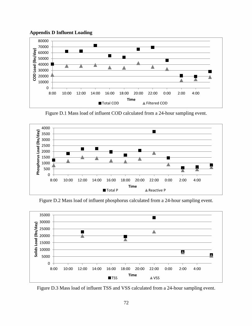
72

Appendix D Influent Loading

Figure D.1 Mass load of influent COD calculated from a 24-hour sampling event.

Figure D.2 Mass load of influent phosphorus calculated from a 24-hour sampling event.

Figure D.3 Mass load of influent TSS and VSS calculated from a 24-hour sampling event.

0

10000

20000

30000

40000

50000

60000

70000

80000

8:00 10:00 12:00 14:00 16:00 18:00 20:00 22:00 0:00 2:00 4:00

CO

D L

oad

(lb

s/d

ay)

Time Total COD Filtered COD

0

500

1000

1500

2000

2500

3000

3500

4000

8:00 10:00 12:00 14:00 16:00 18:00 20:00 22:00 0:00 2:00 4:00

Ph

osp

ho

rus

Load

(lb

s/d

ay)

Time Total P Reactive P

0

5000

10000

15000

20000

25000

30000

35000

8:00 10:00 12:00 14:00 16:00 18:00 20:00 22:00 0:00 2:00 4:00

Solid

s Lo

ad (

lbs/

day

)

Time TSS VSS

73

Appendix E Composite Influent and Grab Effluent COD Analyses

Table E.1 Results from influent and effluent COD analyses

Influent (Composite) Effluent (Grab)

Date

Unfiltered

COD

(mg/L)

Filtered

COD

(mg/L)

Flocculated-

filtered COD

(mg/L)

Unfiltered

COD

(mg/L)

Filtered

COD

(mg/L)

2/3/2014 509.6 291.6 121.6 - -

2/19/2014 572.6 400.6 - - -

3/3/2014 543.8 427.8 167.8 - -

4/18/2014 601.0 371.0 175.5 21.5 18.3

5/14/2014 557.8 326.8 173.8 19.3 20.8

Average 557.0 363.6 159.7 20.4 19.5

SD 33.9 55.0 25.6 1.5 1.6