Study of Parallel Techniques Applied to Surface Reconstruction … · 2017-03-16 · UNIVERSITY OF...
161
UNIVERSITY OF NAVARRA SCHOOL OF ENGINEERING DONOSTIA-SAN SEBASTI ´ AN Study of Parallel Techniques Applied to Surface Reconstruction from Unorganized and Unoriented Point Clouds DISSERTATION submitted for the Degree of Doctor of Philosophy of the University of Navarra by Carlos Ignacio Buchart Izaguirre December 13th, 2010
Transcript of Study of Parallel Techniques Applied to Surface Reconstruction … · 2017-03-16 · UNIVERSITY OF...

UNIVERSITY OF NAVARRA
SCHOOL OF ENGINEERING
DONOSTIA-SAN SEBASTIAN
Study of Parallel Techniques
Applied to Surface Reconstruction
from Unorganized and Unoriented
Point Clouds
DISSERTATIONsubmitted for the
Degree of Doctor of Philosophyof the University of Navarra by
Carlos Ignacio Buchart Izaguirre
December 13th, 2010


A mis abuelos:Opa y NannyPepe y Mima


Agradecimientos
El que da, no debe volver a acordarse;pero el que recibe nunca debe olvidar
Proverbio hebreo
Los agradecimientos suelen ser la parte mas difıcil cuando se escribe lamemoria de la tesis. Por ejemplo, uno no encuentra el orden adecuado, yno quiere dejar a nadie ni siquiera en segundo lugar; el cerebro se estruja amas no poder recordando a todo aquel que nos echo una mano en la tesis(. . .el que recibe nunca debe olvidar); ¡es que algunas veces uno desearıapoder usar un comodın como los empleados en las expresiones regulares[a-zA-Z]+!
Primero que nada quisiera agradecer a mis directores de tesis, Diego yAiert, no solo por el tiempo y esfuerzo que le han dedicado a este trabajo(que tambien valoro enormemente), sino por el tiempo y esfuerzo que mehan dedicado a mı, en mi formacion como investigador y en aquellas horasmas difıciles cuando las cosas parecıan no salir y siempre venıan con unbuen consejo... o un Foster. ¡Gracias!
Mencion honorıfica se la llevan mis padres (Francisco e Ines) y mihermana (Pul... ¡perdon! Titi), que, estando a miles de kilometros dedistancia, han sabido darme siempre una frase de aliento, una llamada enel momento oportuno (o no tan oportuno, pero el carino es lo que cuenta).¡Gracias!
A Jairo, porque entre los dos hemos sacado muchas partes de nuestrastesis y proyectos, por no decir la cantidad de chistes (¿malos?) que tantome han hecho reır estos cuatro anos. ¡Gracias!
Tambien, y de una manera especial, a Alejo Avello, Jordi Vinolas y Luis
iii

iv
Matey. Muchas gracias por darme la oportunidad de desarrollar esta tesisen el CEIT, en el Departamento de Mecanica, en el Area de Simulacion.A Ana Leiza y Begona Bengoetxea, por su ayuda desde los primerısimoscontactos con el CEIT y en todas las gestiones que han ido surgiendo enestos anos. ¡Gracias!
A la Universidad de Navarra, por permitirme cursar mis estudios dedoctorado; al TECNUN, por la formacion profesional, academica y humana,y la ayuda de sus profesores y empleados en el desarrollo de esta tesis y enmis anos como doctorando. ¡Gracias!
Agradecer tambien, de forma conmutativa, a mis companeros yex-companeros de despacho, y del Departamento de Mecanica, todos (deuna u otra forma) han contribuido en el desarrollo de esta tesis (merito porsoportarme en las mananas incluido): Gaizka, Josune, Iker, Hugo, Maite,Angel, Luis U., Jaba, Oskar, Jokin, Inaki G., Javi, Inaki D., Aitor C.,Goretti, Imanol H., Emilio, Yaiza, Sergio, Alberto, Ibon, Alvaro, Denis,Mildred, Aitor R., Miguel, Dimas, Jorge Juan, Manolo, Imanol P., Jorge.¡Gracias!
Estos anos no hubiesen sido igual sin amigos de otros departamentos yde fuera, que le han impreso un caracter “multidisciplinar” a este doctorado:Nirko, Lorena, Jesus, Claudia, Wilfredo, Janelcy, Jose Manuel, Nacho,Elena, Alfredo, Paloma, Fernando, Ioseba, Raul, Manu, Hector, Tomas,Rocıo, Musikalis. ¡Gracias!
Para cerrar, y sin que el hecho de estar en el ultimo parrafo impliqueningun tipo de orden cualitativo, muchas gracias a Patric, Jesus, Jose Luis,Rober, Karmele, Paqui, Patxi, Josemi, Franklin, Enrique, Alvaro, Dani,Hector, Josetxo, Noelia, Marycarmen, por tantos pequenos (y grandes)favores. ¡Gracias!
¡Ah! Por si se me olvida alguien: ¡muchas gracias [a-zA-Z]+! ;)

Abstract
Nowadays, digital representations of real objects are becoming biggeras scanning processes are more accurate, so the time required for thereconstruction of the scanned models is also increasing.
This thesis studies the application of parallel techniques in the surfacereconstruction problem, in order to improve the processing time requiredto obtain the final mesh. It is shown how local interpolating triangulationsare suitable for global reconstruction, at the time that it is possible totake advantage of the independent nature of these triangulations to designhighly efficient parallel methods.
A parallel surface reconstruction method is presented, based on localDelaunay triangulations. The input points do not present any additionalinformation, such as normals, nor any known structure. This method hasbeen designed to be GPU friendly, and two implementations are presented.
To deal the inherent problems related to interpolating techniques (suchas noise, outliers and non-uniform distribution of points), a consolidationprocess is studied and a parallel points projection operator is presented, aswell as its implementation in the GPU. This operator is combined with thelocal triangulation method to obtain a better reconstruction.
This work also studies the possibility of using dynamic reconstructiontechniques in a parallel fashion. The method proposed looks for a betterinterpretation and recovery of the shape and topology of the target model.
v

vi
Resumen
Hoy en dıa, las representaciones digitales de objetos reales se van haciendomas grandes a medida que los procesos de escaneo son mas precisos, por loque el tiempo requerido para la reconstruccion de los modelos escaneadosesta tambien aumentando.
Esta tesis estudia la aplicacion de tecnicas paralelas al problemade reconstruccion de superficies, con el objetivo de mejorar los tiemposrequeridos para obtener el mallado final. Tambien se muestra como lastriangulaciones locales interpolantes son utiles en reconstrucciones globales,y que es posible sacar partido de la naturaleza independiente de estas paradisenar metodos paralelos altamente eficientes.
Se presenta un metodo paralelo de reconstruccion de superficies, basadoen triangulaciones locales de Delaunay. Los puntos no estan estructurados nitienen informacion adicional, como normales. Este metodo ha sido disenadoteniendo en mente la GPU, y se presentan dos implementaciones.
Para contrarrestar los problemas inherentes a las tecnicas interpolantes(ruido, outliers y distribuciones no uniformes), se ha estudiado un procesode consolidacion de puntos y se presenta un operador paralelo de proyeccion,ası como su implementacion en la GPU. Este operador se ha combinado conel metodo de triangulacion local para obtener una mejor reconstruccion.
Este trabajo tambien estudia la posibilidad de usar tecnicas dinamicasde una forma paralela. El metodo propuesto busca una mejor interpretaciony captura de la forma y la topologıa del modelo.
vii

viii

Contents
I Introduction 1
1 Introduction 3
1.1 Applications . . . . . . . . . . . . . . . . . . . . . . . . . . . 6
1.2 Data acquisition . . . . . . . . . . . . . . . . . . . . . . . . 7
1.3 Objectives . . . . . . . . . . . . . . . . . . . . . . . . . . . . 8
1.4 Dissertation organization . . . . . . . . . . . . . . . . . . . 10
2 State of the art 11
2.1 Interpolating methods . . . . . . . . . . . . . . . . . . . . . 12
2.1.1 Delaunay triangulation . . . . . . . . . . . . . . . . . 12
2.1.2 Local triangulations . . . . . . . . . . . . . . . . . . 14
2.2 Approximating methods . . . . . . . . . . . . . . . . . . . . 16
2.3 Parallel triangulations . . . . . . . . . . . . . . . . . . . . . 18
2.3.1 Hardware accelerated algorithms . . . . . . . . . . . 19
II Proposal 21
3 GPU Local Triangulation 23
3.1 Introduction . . . . . . . . . . . . . . . . . . . . . . . . . . . 24
3.2 Sampling criteria . . . . . . . . . . . . . . . . . . . . . . . . 25
3.3 Description of the method . . . . . . . . . . . . . . . . . . . 25
ix

x CONTENTS
3.3.1 Preprocess phase – Computing the k-NN . . . . . . 25
3.3.1.1 k-NN based on clustering techniques . . . . 26
3.3.1.2 k-NN using kd-trees . . . . . . . . . . . . . 27
3.3.1.3 Final comments . . . . . . . . . . . . . . . 27
3.3.2 Parallel triangulation . . . . . . . . . . . . . . . . . . 27
3.3.3 Phase 1 – Normal estimation . . . . . . . . . . . . . 28
3.3.3.1 Normals orientation . . . . . . . . . . . . . 30
3.3.4 Phase 2 – Projection . . . . . . . . . . . . . . . . . . 31
3.3.5 Phase 3 – Angle computation . . . . . . . . . . . . . 32
3.3.6 Phase 4 – Radial sorting . . . . . . . . . . . . . . . . 33
3.3.7 Phase 5 – Local triangulation . . . . . . . . . . . . . 33
3.3.7.1 2D validity test . . . . . . . . . . . . . . . 34
3.3.7.2 Proof . . . . . . . . . . . . . . . . . . . . . 36
3.4 Implementation using shaders . . . . . . . . . . . . . . . . . 37
3.4.1 Initial texture structures overview . . . . . . . . . . 38
3.4.2 Texture assembly . . . . . . . . . . . . . . . . . . . . 41
3.4.3 Phase 1 – Normal estimation . . . . . . . . . . . . . 41
3.4.4 Phases 2 and 3 – Projection and angle computation 42
3.4.5 Phase 4 – Radial sorting . . . . . . . . . . . . . . . . 42
3.4.6 Phase 5 – Local triangulation . . . . . . . . . . . . . 44
3.5 Implementation using CUDA . . . . . . . . . . . . . . . . . 45
3.5.1 Data structures . . . . . . . . . . . . . . . . . . . . . 46
3.5.2 Phase 4 – Radial sorting . . . . . . . . . . . . . . . . 48
3.5.3 Phase 5 – Local triangulation . . . . . . . . . . . . . 48
3.6 Experiments and results . . . . . . . . . . . . . . . . . . . . 48
3.6.1 CPU vs Shaders vs CUDA . . . . . . . . . . . . . . 50
3.6.2 Reconstruction results . . . . . . . . . . . . . . . . . 53
3.6.3 Big models . . . . . . . . . . . . . . . . . . . . . . . 57
3.6.4 Comparison with an approximating method . . . . . 58
3.6.5 Application in the medical field . . . . . . . . . . . . 61
3.6.6 Application in cultural heritage . . . . . . . . . . . . 61
3.7 Discussion . . . . . . . . . . . . . . . . . . . . . . . . . . . . 64

CONTENTS xi
4 Parallel Weighted Locally Optimal Projection 65
4.1 Previous works . . . . . . . . . . . . . . . . . . . . . . . . . 65
4.1.1 Locally Optimal Projection Operator . . . . . . . . . 66
4.1.2 Weighted Locally Optimal Projection Operator . . . 67
4.2 Parallel WLOP . . . . . . . . . . . . . . . . . . . . . . . . . 68
4.2.1 Implementation details . . . . . . . . . . . . . . . . . 71
4.3 Experiments and results . . . . . . . . . . . . . . . . . . . . 71
4.4 Discussion . . . . . . . . . . . . . . . . . . . . . . . . . . . . 77
5 Hybrid surface reconstruction: PWLOP + GLT 79
5.1 Improving the input data set through points consolidation . 79
5.2 Results . . . . . . . . . . . . . . . . . . . . . . . . . . . . . . 80
5.3 Discussion . . . . . . . . . . . . . . . . . . . . . . . . . . . . 87
6 Study of multi-balloons reconstruction 89
6.1 Dynamic techniques . . . . . . . . . . . . . . . . . . . . . . 89
6.1.1 Classic balloons . . . . . . . . . . . . . . . . . . . . . 91
6.2 Multi-balloons . . . . . . . . . . . . . . . . . . . . . . . . . 93
6.2.1 Scalar function fields . . . . . . . . . . . . . . . . . . 95
6.2.2 Evolution process . . . . . . . . . . . . . . . . . . . . 96
6.2.2.1 Global and local fronts . . . . . . . . . . . 96
6.2.2.2 Two-step evolution . . . . . . . . . . . . . 98
6.2.2.3 Gradient modulation term: κi . . . . . . . 99
6.2.2.4 Local adaptive remeshing . . . . . . . . . . 100
6.2.3 Topology change . . . . . . . . . . . . . . . . . . . . 104
6.2.3.1 Genus . . . . . . . . . . . . . . . . . . . . . 104
6.2.3.2 Holes . . . . . . . . . . . . . . . . . . . . . 106
6.3 Experiments and results . . . . . . . . . . . . . . . . . . . . 106
6.4 Discussion . . . . . . . . . . . . . . . . . . . . . . . . . . . . 109

xii CONTENTS
III Conclusions 111
7 Conclusions and future work 113
7.1 Conclusions . . . . . . . . . . . . . . . . . . . . . . . . . . . 113
7.2 Future research lines . . . . . . . . . . . . . . . . . . . . . . 115
IV Appendices 117
A GPGPU computing 119
A.1 Shaders . . . . . . . . . . . . . . . . . . . . . . . . . . . . . 120
A.2 CUDA . . . . . . . . . . . . . . . . . . . . . . . . . . . . . . 122
A.2.1 CUDA Program Structure . . . . . . . . . . . . . . . 123
A.2.2 Occupancy . . . . . . . . . . . . . . . . . . . . . . . 124
A.2.3 CUDA Memory Model . . . . . . . . . . . . . . . . . 124
B Generated Publications 127
Index 129
References 131
List of Figures
1.1 Different point clouds . . . . . . . . . . . . . . . . . . . . . 3
1.2 Noisy set of points . . . . . . . . . . . . . . . . . . . . . . . 4
1.3 Ambiguities are commonly present in points from a scannedsurface . . . . . . . . . . . . . . . . . . . . . . . . . . . . . . 4
1.4 Example of a points cloud extracted from a computertomography . . . . . . . . . . . . . . . . . . . . . . . . . . . 7
1.5 3dMface System, used in face scanning . . . . . . . . . . . . 8
1.6 Creaform REVscan laser scanner, used in reverse engineering 9
2.1 Voronoi diagrams and Delaunay triangulations . . . . . . . 13
2.2 Comparison between different local triangulation methods . 15
2.3 Intersection configurations for Marching Cubes . . . . . . . 18
2.4 Performance evolution comparison between CPUs and GPUs 19
3.1 Flow diagram of the proposed reconstruction algorithm . . 24
3.2 Normal estimation using PCA and wPCA . . . . . . . . . . 29
3.3 Minimal rotation . . . . . . . . . . . . . . . . . . . . . . . . 31
3.4 The is valid function verifies if a point belongs to a partialVoronoi region. . . . . . . . . . . . . . . . . . . . . . . . . . 35
3.5 The validity test is local and must be performed several timesto obtain the local triangulation of a point . . . . . . . . . . 35
3.6 is valid never invalidates Voronoi neighbors . . . . . . . . . 36
3.7 Flow diagram of the shaders implementation . . . . . . . . 38
3.8 TP and TN – Points and normals textures . . . . . . . . . . 39
xiii

xiv LIST OF FIGURES
3.9 TQ – Candidate points texture . . . . . . . . . . . . . . . . 40
3.10 TI – Index table texture . . . . . . . . . . . . . . . . . . . . 41
3.11 Tα – Angles texture: similar to the TQ structure but replacingthe distance with the angle . . . . . . . . . . . . . . . . . . 42
3.12 TQ′ – Projected candidate points texture . . . . . . . . . . . 42
3.13 The shaders implementation of GLT uses a ring to check allthe neighbors in parallel, discarding the invalid ones in eachiteration . . . . . . . . . . . . . . . . . . . . . . . . . . . . . 46
3.14 TR – Delaunay ring texture . . . . . . . . . . . . . . . . . . 46
3.15 Flow diagram of the CUDA implementation . . . . . . . . . 47
3.16 Time comparison of the computation of the neighborhoods 51
3.17 Time comparison of the normal estimation phase . . . . . . 51
3.18 Time comparison of the angle computation and projectionphase . . . . . . . . . . . . . . . . . . . . . . . . . . . . . . 51
3.19 Time comparison of the sorting phase . . . . . . . . . . . . 52
3.20 Time comparison of the local Delaunay validation . . . . . . 52
3.21 Time comparison of the local Delaunay triangulation . . . . 52
3.22 Comparison between the different proposed reconstructionmethods . . . . . . . . . . . . . . . . . . . . . . . . . . . . . 53
3.23 Horse model rendered along with its wireframe . . . . . . . 54
3.24 Neck and chest detail of the Horse model . . . . . . . . . . 54
3.25 A synthetic model . . . . . . . . . . . . . . . . . . . . . . . 55
3.26 Running shoe along with its wireframe . . . . . . . . . . . . 55
3.27 Blade model . . . . . . . . . . . . . . . . . . . . . . . . . . . 56
3.28 Top view of the Blade model . . . . . . . . . . . . . . . . . 56
3.29 Overall view of time consumption in the reconstruction ofthe Asian Dragon model (3609K points) . . . . . . . . . . . 57
3.30 Comparison with the Poisson reconstruction - Angel . . . . 59
3.31 Comparison with the Poisson reconstruction - Happy Buddha 59
3.32 Comparison with the Poisson reconstruction - Blade . . . . 60
3.33 Comparison with the Poisson reconstruction - Interior detailof the Blade model . . . . . . . . . . . . . . . . . . . . . . . 60
3.34 Patients’ Heads models . . . . . . . . . . . . . . . . . . . . . 61

LIST OF FIGURES xv
3.35 Reconstruction of a Trophy . . . . . . . . . . . . . . . . . . 62
3.36 Reconstruction of a Theatre . . . . . . . . . . . . . . . . . . 63
3.37 Reconstruction of a Tower . . . . . . . . . . . . . . . . . . . 63
4.1 Local support neighborhood vs. the extended LSN . . . . . 69
4.2 Speed comparison between WLOP, eWLOP and PWLOPwith the Stanford Bunny . . . . . . . . . . . . . . . . . . . . 72
4.3 Projection of the Happy Buddha model using a randominitial guess . . . . . . . . . . . . . . . . . . . . . . . . . . . 73
4.4 Projection of the Happy Buddha model using anapproximation from spatial subdivision techniques . . . . . 74
4.5 Projection of different data sets using WLOP, eWLOP andPWLOP . . . . . . . . . . . . . . . . . . . . . . . . . . . . . 75
4.6 The extended LSN computation times are common for boththe eWLOP and PWLOP . . . . . . . . . . . . . . . . . . . 75
4.7 The computation of the extended LSN is the same for theeWLOP and PWLOP . . . . . . . . . . . . . . . . . . . . . 76
4.8 Projection of the Happy Buddha model resetting the initialdata set . . . . . . . . . . . . . . . . . . . . . . . . . . . . . 76
5.1 Stanford Dragon . . . . . . . . . . . . . . . . . . . . . . . . 81
5.2 Asian Dragon . . . . . . . . . . . . . . . . . . . . . . . . . . 82
5.3 Happy Buddha . . . . . . . . . . . . . . . . . . . . . . . . . 82
5.4 Hand model reconstruction comparison . . . . . . . . . . . . 83
5.5 Hand model detail comparison . . . . . . . . . . . . . . . . 83
5.6 Noisy Foot with 20K points . . . . . . . . . . . . . . . . . . 84
5.7 Comparison of the hybrid PWLOP + GLT with the Poissonreconstruction . . . . . . . . . . . . . . . . . . . . . . . . . . 85
5.8 Results of the hybrid PWLOP + GLT reconstruction . . . . 86
5.9 Multi-resolution Happy Buddha using the hybrid approach 88
6.1 Competing fronts . . . . . . . . . . . . . . . . . . . . . . . . 91
6.2 Level sets . . . . . . . . . . . . . . . . . . . . . . . . . . . . 91
6.3 Flow diagram of the studied reconstruction using multiballoon 94

xvi LIST OF FIGURES
6.4 Multiple seeds placed in the Hand model . . . . . . . . . . . 95
6.5 Multi-resolution grid used as satisfaction function . . . . . . 97
6.6 Slice of the Horse model’s distance function . . . . . . . . . 97
6.7 Uniform vs. Local adaptive remeshing . . . . . . . . . . . . 102
6.8 Detail of the effects of the local adaptive remeshing . . . . . 103
6.9 Topology change . . . . . . . . . . . . . . . . . . . . . . . . 105
6.10 Rconstruction of a high-genus synthetic model . . . . . . . 105
6.11 Multiple balloons evolving to reconstruct the Hand model . 107
6.12 Reconstruction of the Stanford Dragon model . . . . . . . . 107
6.13 Reconstruction stages for the Stanford Dragon model . . . . 108
6.14 Reconstruction of the Horse model . . . . . . . . . . . . . . 108
A.1 Thread hierarchy. . . . . . . . . . . . . . . . . . . . . . . . . 123
A.2 Memory hierarchy. . . . . . . . . . . . . . . . . . . . . . . . 125

List of Tables
3.1 Total reconstruction time using three differentimplementations . . . . . . . . . . . . . . . . . . . . . . . . 50
3.2 Total reconstruction time of big models . . . . . . . . . . . 57
3.3 Comparison with the Poisson reconstruction method . . . . 58
4.1 Speed comparison between WLOP, eWLOP and PWLOPwith the Happy Buddha model . . . . . . . . . . . . . . . . 75
5.1 Comparison between the proposed hybrid approach and thePoisson reconstruction method . . . . . . . . . . . . . . . . 84
xvii

xviii LIST OF TABLES

List of Algorithms
3.1 Local Delaunay triangulation in 2D . . . . . . . . . . . . . . 343.2 Adapted Bitonic Merge Sort for multiple lists sorting . . . . 443.3 Local Delaunay triangulation algorithm adapted for its
implementation with shaders. . . . . . . . . . . . . . . . . . 453.4 Local Delaunay Triangulation algorithm optimized for CUDA. 496.1 Overview of the algorithm proposed. . . . . . . . . . . . . . 946.2 Local adaptive remeshing operator . . . . . . . . . . . . . . 102
xix

xx LIST OF ALGORITHMS

Part I
Introduction


Chapter 1
Introduction
Science brings men nearer to God
Louis Pasteur
Surface reconstruction from a set of points is an amazing field of work dueto the uncertainty nature of the problem. It is well known in computergraphics. It has been formally defined as given a set of points P which aresampled from a surface S in R3, construct a surface S so that the points ofP lie on S (Gopi et al., 2000), assuming there are neither outliers nor noisypoints, i.e., it defines an interpolating reconstruction. The resulting surfaceS usually is a triangle mesh, a discrete representation of the real surface.If noise is present in the set of points (P is near S), an approximatingreconstruction is needed in order to avoid interference caused by points outof the surface. Some examples of input points can be seen in Figure 1.1while Figure 1.2 shows a noisy dataset.
Figure 1.1: Different point clouds.
It is easy to see that surface reconstruction faces several problems:incomplete data, inconsistencies, noise, data size, ambiguities (see Figure1.3). It is a vast researching area, and many methods have been already
3

4 Chapter 1. Introduction
Figure 1.2: Noisy set of points.
proposed. Despite the work that has been done in this field, the correctgeneration of a triangle mesh from a points cloud is still a study goaltrying to improve drawbacks current techniques have. Also, it is still anopen field because it is too complex, and probably impossible, to fullyrecovery an unknown surface without previously assuming some kind ofinformation, such as normals’ direction and orientation, presence of holes orsharp features, and the topology of the model. Almost every single existingmethod relies in at least one parameter (for example, the sampling rate),and is usually focused in a subset of problems, so it can better exploit theimplicit model’s characteristics in order to obtain a proper reconstruction.
Figure 1.3: Ambiguities are commonly present in points from ascanned surface. For example, the top of this piece is a cylinder,but in some zones there where no points scanned, leading toseveral interpretations of the data.
Today’s improvements in acquisition methods and computers, alongwith the demand for more detailed models, have led up to work, more

5
and more, with larger point clouds, increasing the reconstruction time andmemory requirements. This have lead to develop more efficient algorithmsin terms of memory and processing time.
Nowadays, the general evolution of the hardware and software is morefocused on the distribution of the processing load than in the increment ofthe individual computing power. This tend can be found in many areas:search engines, numerical simulation, cryptography, movies rendering, etc.,where parallel algorithms have been developed to take advantage of themodern hardware. For example, thanks to their high parallelization level, asingle graphic card usually have more processing power than a top-lineCPU. More on, since a few years ago it is common to find multi-coreprocessors in personal computers, as well as powerful graphic cards, soit is no more a restricted field that requires high budgets. The parallelprogramming would offer a way to solve the dataset size issue, since thepoints processing can be split among different processors or computingnodes, also reducing the individual memory requirements of each computer.
Talking about the graphics hardware field, in recent years thattechnology has allowed developers to execute custom programs in theGPU (Graphics Processing Unit), taking advantage of the huge processingpower it offers, in the so called GPGPU programming (General PurposeGPU )1. Although by the time this thesis is being presented another GPUsurface reconstruction method has been proposed, the migration of anyalgorithm to the GPU is not trivial and usually requires a high numberof modifications. At the same time, not every existing technique can beimplemented in parallel, and even less in the GPU, being necessary in suchcases, the creation of new processing paradigms. Finally, the GPU methodmentioned above corresponds to an approximating reconstruction and, asit will be seen later, this work proposes an interpolating approach.
Another interesting and common fact about surface reconstruction isthat there is not always a need for real-time reconstruction. Usually, thereconstruction is a preprocess for a later application, and then, does notnecessarily have to be a fully automatic and real-time process. The user canguide the reconstruction or, as usually happens, can perform modificationsto the resulting surface to correct any problem (such as holes filling) orinclude information the reconstruction process did not have access to (zonesthat could not be scanned, or solve ambiguities in the set of points). In any
1For more information about GPGPU programming, please refer to Appendix A.

6 Chapter 1. Introduction
case, although real-time is not a must in these cases, efficiency should betaken into account due to the size of data sets increases continually (mostof the models have hundred of thousand points or even a few million).
The present work is mainly focused in parallelization. It studiesthe possibility of the design and implementation of parallel surfacereconstruction techniques, and especially in their implementation in graphichardware for a even higher speed boost. The vast processing power ofcurrent GPUs makes them highly desirable targets in terms of executiontime of the reconstruction.
1.1 Applications
Surface reconstruction finds very useful applications in the industry inthe fields of reverse engineering and CAD (Computer Aided Design). Inthis case, it is more common to use parametric surface patches instead ofpolygonal meshes to represent the reconstructed object.
Another important area of use is in movies and videogames production,where figures modeled in clay are digitalized to be later included into themedia content.
Also, it is widely used in cultural heritage allowing the digitalization ofsculptures, vases, historical sites, etc. for analysis, documentation or publicexposition. For example, the engrave of an old ceil may be digitalized forits study in a more comfortable place and to avoid that its manipulationmay deteriorate the engrave. Some examples of surface reconstruction inthis field can be found in (Besora et al., 2008; Cano et al., 2008; Torreset al., 2009a).
In medicine, surface reconstruction provides a practical way to visualizecertain kinds of tissues (Figure 1.4), as well as to extract an interactionsurface to be used in simulators. It is also possible, for example, to supplantdental casts with 3D models of the teeth for dental prosthetics (bridges,crowns, etc).

Section 1.2. Data acquisition 7
Figure 1.4: Example of a points cloud extracted from a computertomography.
1.2 Data acquisition
The process to convert a real surface into a digital representation startswith the acquisition of a set of points that represents it. This process iscalled surface scanning, and the tools that acquires the points, scanners.Among the different kinds of scanners, some of the most common onesinclude:
• Image-based scanners: these scanners consist of at least a coupleof calibrated cameras that capture the object from different points ofview. These images are used to compute a view point dependent 3Dset of points using a correspondence analysis, as described in (Jones,1995). Figure 1.5 shows a face scanner.
• Time-of-flight scanners: by measuring the round-trip time of apulse of light emitted to the object it is possible to compute thedistance to it. Their main disadvantage is that they can detect onlyone point in their view direction, so either the laser must be moved,the object rotated or a mirror used to capture the back faces of anobject.
• Hand-held laser scanners: these scanners project a laser line or dotonto the object, and the distance to it is measured by the scanner.An example of these scanners is shown in Figure 1.6.

8 Chapter 1. Introduction
• Contact scanners: this kind of scanners probe the object throughphysical touch and are very precise. Their main disadvantage is thatthe object must be touched, and in some cases it is not possible or itis not easy. Also, physical contact with the object may damage it.
Figure 1.5: 3dMface System, used in face scanning.
Finally, some other acquisition techniques include segmentation ofmedical images, data from simulations and video processing. The lattermakes use of similar techniques to image based scanning, by replacing themulti-camera sources with a multi-view approach (epipolar geometry) andtracking 2D feature points along the video sequence taking advantage of thetemporal coherence (for more information about this kind of techniques,please refer to (Sanchez et al., 2010)).
1.3 Objectives
As has been stated before, surface reconstruction is a vast research areathat has been addressed from different points of view, but that remainsopen given the uncertain nature of the problem. Even more, some of themost reliable methods proposed depend on additional data such as normalorientation, that is not always available during the reconstruction process.Surface reconstruction methods should be able to take advantage of theadditional information if it is present, but should not be dependent on it.
Additionally, the size of the point clouds is rapidly increasing, making

Section 1.3. Objectives 9
Figure 1.6: Creaform REVscan laser scanner, used in reverseengineering.
necessary the design of fast methods that can handle such amount of data.Parallel programming is presented as a very powerful solution. More on,GPGPU programming has helped in recent years to a dramatic speedincrease in many fields. It is reasonable, then, to think that techniquesdeveloped should be implementable in the GPU.
For all this, the main objective of this thesis is the study of paralleltechniques applied to the design of surface reconstruction algorithmsfrom unorganized and unoriented sets of points, and additionally, theoptimization of existing reconstruction supporting methods and theimplementation and acceleration of studied algorithms using commoditygraphic hardware.
The following specific objectives are intended to limit the scope of thethesis and focus the contributions of the work:
• Input data: although many surface scanners exist, not every systemprovides additional information from the digitalized object, so themethod should be able to work without it. The input data, then,should consists in a set of points in 3D without any kind of structureor additional information. Also, the number of parameters should beas minimal as possible to make more flexible the use of the developedmethods in automatic processes.
• Noise tolerance: the methods studied should be robust againstnoise. Given that some techniques are non-tolerant to noise by

10 Chapter 1. Introduction
their nature (e.g. interpolating techniques), it is convenient to studyauxiliary techniques that may help to overcome this limitation. Eventhough, the goal is not to treat with high levels of noise.
• Scalability: as point clouds are becoming more and more large, themethods studied should be able to scale over the time in order to beuseful even when the dimensionality of the datasets overpasses thesize of current models.
Finally, the hardware employed in this project is restricted tocommodity PCs and graphic cards of the same level. It is not pretended tobe a study of surface reconstruction on PC clusters, large computing farmsor specialized computers.
1.4 Dissertation organization
The rest of this memory is organized as follows. Chapter 2 reviews themost important reconstruction techniques. Chapter 3 presents the studyof a surface reconstruction based on local Delaunay triangulations and itsimplementation in the GPU. Chapter 4 discusses a projection operator forpoints consolidation as well as a new parallel approach. This operator iscombined with the surface reconstruction method proposed; this hybridtechnique is described in Chaper 5. In Chapter 6 a different reconstructionapproach, based in multiple active contours, is studied. Experimentalresults are shown at the end of each chapter. Finally, Chapter 7 showsthe conclusions of this thesis, and it also comments possible future lines ofwork.

Chapter 2
State of the art
Science, my lad, is made up of mistakes,but there are mistakes which it is useful to make,
because they lead little by little to the truth
Jules Verne
Surface reconstruction is an active research field, and many works havebeen presented, which can be classified using different approaches1. On onehand, if it is assumed that the points have no noise, i.e., they belong to thesurface, then it is sufficient to find a relationship among the points (theirconnectivity) to reconstruct a discrete representation of the surface. Thesekinds of techniques are called interpolating. On the other hand, if noiseor incomplete data is present, approximating techniques are required. Thelatter usually rely on implicit functions to define a similar surface whilebalancing outliers, noise and high details. Additionally, it is not uncommonfor many methods, to filter the point set as a preprocess step, in order toimprove it (removing outliers, for example). Also, some other techniquesexist, called dynamic techniques, but they are discussed in Chapter 6.
The rest of this section will describe some of the most importantworks related to surface reconstruction, as well as a discussion on paralleltechniques and GPU methods. The third classification mentioned above iscommented separately in Section 6.1.
1For convenience, a classification similar to that employed in (Gopi et al., 2000) isused.
11

12 Chapter 2. State of the art
2.1 Interpolating methods
Interpolating methods rely on points that effectively are on the originalsurface. Although they are not robust against noise and outliers, thequality of the reconstructed mesh is usually better than those generated byapproximating methods, given a noise free dataset. This quality representsboth triangle proportions, and fidelity to the target surface.
The main weakness of interpolating methods is the presence of noiseand outliers. It is interesting to note that isolate outliers are usuallydiscarded without any additional work given proper neighborhood sizes.Sampling inaccuracies on the other hand, usually fall into the local supportof interpolating methods and are included in the reconstruction. Undercertain levels of noise, just a rough surface is obtained. In worse cases,however, the reconstruction method may fail to create a consistent surface.
2.1.1 Delaunay triangulation
Maybe the most known and common interpolating technique is theDelaunay triangulation, initially introduced by (Delaunay, 1934) (Figure2.1). Given a set of points P in the d-dimensional Euclidean space, theDelaunay triangulation DT (P ) is such that no point p ∈ P is inside thecircum-hypersphere of any d-simplex2 in P . It is important to commentthat if the set of points P is in a 3-dimensional space, DT (P ) is not asurface but a tetrahedral mesh, so a post-process is required to extract theon-surface triangles from the full triangulation. Unless explicitly mentioned,the rest of this work assumes d = 3.
The DT (P ) is also the dual of the Voronoi diagram of P ,where consecutive nodes of the Voronoi diagram are connected in thetriangulation. The Voronoi region of a point p ∈ P is given by all pointsthat are nearer to p than to any other point of P (see Figure 2.1). Thisproperty is often used to construct either the Delaunay triangulation or theVoronoi diagram based on the other one.
Finally, the local triangulation of a point pi is defined as the set oftriangles that have pi as a vertex. Given the local Delaunay triangulations
2A d-simplex is the minimum object in a Ed, the d-dimensional analogue of a triangle(which is the 2-simplex, for d = 2). A 3-simplex is, therefore, a tetrahedra.

Section 2.1. Interpolating methods 13
(LDT ) of every point in P , the global triangulation can be constructed asfollows:
DT (P ) =⋃pi∈P
LDT (pi) (2.1)
Figure 2.1: Voronoi diagrams and Delaunay triangulations areduals.
A good example of Delaunay triangulations in surface reconstructionis presented by (Attene and Spagnuolo, 2000). In this work, the Delaunaytetrahedralization of the input points is constructed and then, by the use ofan Euclidean minimum spanning tree and a Gabriel graph3, the boundaryof the surface is obtained.
One of the most cited Delaunay based reconstructions is the PowerCrust method proposed by (Amenta et al., 2001). It constructs the Voronoidiagram of the input points, and then extracts a polygonal mesh using theinverse of the medial axis transform obtained from the Voronoi diagram.The medial axis of an object is a tool for shape description and consistsin the closure of the locus of the centers of all maximal inscribed discs inthe target surface. The medial axis transform is the medial axis together
3A Gabriel graph is a subset of the Delaunay triangulation, where two points p, q ∈ Pare connected if the closed disc which diameter is the line segment pq contains no pointsfrom P .

14 Chapter 2. State of the art
with the radius of the maximal inscribed circle center in each point on themedial axis (Vermeer, 1994).
The Cocone algorithm (Amenta et al., 2000) also relies on Voronoiregions for the reconstruction. It extracts the reconstructed surfaced byfiltering the triangulation as follows: for a sample point p ∈ P and a Voronoiedge e in the Voronoi cell of p, if for the Voronoi cells adjacent to e have apoint x such that the vector px makes a right angle with the normal of p,then the dual of the Voronoi cells is included in the reconstruction. Someother improvements to this method have been presented, concretely theTight Cocone (Dey and Goswami, 2003), basically a hole-filling extension;and the Robust Cocone (Dey and Goswami, 2006), that incorporatestolerance against noisy inputs.
In (Allegre et al., 2007) a progressive method is shown, where thedata set is simplified at the time it is selective reconstructed using pointinsertions and deletions in the Delaunay triangulation. At the end, theresolution of the resulting mesh is locally adapted to satisfy the featuresizes of the model.
2.1.2 Local triangulations
Previously mentioned techniques are based in global triangulationsalgorithms, but (Linsen and Prautzsch, 2001) show that local triangulationsare also well suited for surface reconstruction and can lead to fasteralgorithms, even more if the main purpose of the reconstruction is thevisualization of a polygonal mesh rather than its utilization in laterprocessing tasks. Assuming a well sampled surface, (Linsen and Prautzsch,2001) construct a triangles fan around each point using its 6-neighborhood.
For example, assuming a dense sampling of the original object, (Gopiet al., 2000) show that the neighborhood of p is the same as its projectiononto the tangent plane of p, given that the distance to p is maintained.Based on this, a lower dimensional Delaunay triangulation is done in 2D,resulting in a faster reconstruction than in 3D (as was previously mentioned,the 3D Delaunay triangulation is composed of tetrahedra rather thantriangles). The final mesh is obtained by merging all individual fans.
Another technique, very similar to local triangulations, are the useof advancing frontal techniques (AFT). An AFT starts with a minimal
Section 2.1. Interpolating methods 15
subset of the final reconstruction and expands its boundaries iterativelycovering the whole surface. Current methods based on advancing frontsperform such iterations one point at a time (here their similarity to localtriangulations). For example, (Bernardini et al., 1999) start with a seedtriangle and adds subsequent triangles using a ball pivoted around theedges of the boundaries of mesh, and (Crossno and Angel, 1999) use alocalized triangulation approach, called Spiraling Edge, in which a pointis not marked as finished until it is completely surrounded by triangles(exceptions are boundary points).
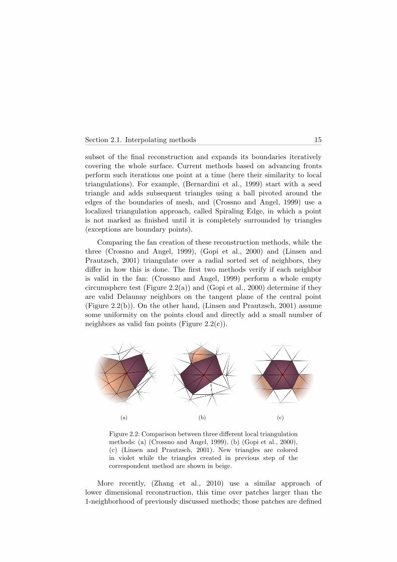
Comparing the fan creation of these reconstruction methods, while thethree (Crossno and Angel, 1999), (Gopi et al., 2000) and (Linsen andPrautzsch, 2001) triangulate over a radial sorted set of neighbors, theydiffer in how this is done. The first two methods verify if each neighboris valid in the fan: (Crossno and Angel, 1999) perform a whole emptycircumsphere test (Figure 2.2(a)) and (Gopi et al., 2000) determine if theyare valid Delaunay neighbors on the tangent plane of the central point(Figure 2.2(b)). On the other hand, (Linsen and Prautzsch, 2001) assumesome uniformity on the points cloud and directly add a small number ofneighbors as valid fan points (Figure 2.2(c)).
(a) (b) (c)
Figure 2.2: Comparison between three different local triangulationmethods: (a) (Crossno and Angel, 1999), (b) (Gopi et al., 2000),(c) (Linsen and Prautzsch, 2001). New triangles are coloredin violet while the triangles created in previous step of thecorrespondent method are shown in beige.
More recently, (Zhang et al., 2010) use a similar approach oflower dimensional reconstruction, this time over patches larger than the1-neighborhood of previously discussed methods; those patches are defined

16 Chapter 2. State of the art
as regions where point’s tangent planes have small variations.
2.2 Approximating methods
If either noise or outliers are present in the input data, interpolatingtechniques fail to generate a correct reconstruction, because all the pointsare taken into account for the triangulation, interpreting noise as fine detailsof the target surface.
Approximating techniques tend to solve this issue at the cost oflosing detail. It is also true that many methods can achieve good qualityreconstructions, but usually incurring in a high memory consumption. Inthis sense, local triangulations, such as the studied in the previous section,can reduce their memory footprint by subdividing the reconstruction intosmaller blocks.
Among approximating reconstructions can be found many differentapproaches, but most of them are based on the construction of an implicitfunction I(x). This function is commonly represented as a scalar fieldusing spatial subdivision techniques, such as voxels or octrees. In this way,the surface reconstruction is transformed into an iso-surface extractionproblem: most of the methods use functions such that S is defined byI(x) = 0 (for example, if I(x) is a distance function). The robustness andquality of these algorithms are determined by the volume generation andthe precision of the iso-surface when compared with the original surface,i.e., the resolution of the implicit function.
One of the first methods presented in this area was the work of (Hoppeet al., 1992). It computes a signed distance field from the points to theirtangent planes. Such planes are estimated from the local neighborhoodof each point using principal component analysis, and re-oriented using aconnectivity graph to consistently propagate a common orientation.
(Bajaj et al., 1995) use α-shapes to determine the signed distancefunction. Given the Delaunay triangulation DT (P ) of P , an α-shape is, asa general idea, the subset of simplices of DT (P ) smaller than the selectedvalue α. All the simplices that belong to the α-shape are marked as internal,while the others are marked as external. With this space classification thesigned function is constructed.

Section 2.2. Approximating methods 17
(Ohtake et al., 2005) make use of weighted local shape functions inan adaptive fashion to create a global approximation, and (Nagai et al.,2009) follow a similar idea, introducing a Laplacian smoothing term basedon the diffusion of the gradient field. Alternatively, (Samozino et al., 2006)center compactly supported radial basis functions in a filtered subset of theVoronoi vertices of the input points.
Using the Voronoi diagram of the input points, (Alliez et al., 2007)compute a tensor field and estimates from it the normals of the points. Bysolving a generalized eigenvalue problem, it computes an implicit functionwhich gradients are most aligned with the principal axes of the tensor field.
Using a different approach, (Esteve et al., 2008) compute a piecewisetricubic Bspline surface from the discrete membrane (a collection offace-connected voxels that is derived from the points set). This algebraicsurface is iteratively adjusted to the discrete membrane, adjusting thecontinuity between voxels and fitting the isosurface to the center ofhard-tagged voxels (that contain input points).
Several approximating techniques have been based on physicalphenomena. For example, (Jalba and Roerdink, 2006) aggregate points intoa grid and convert the non-empty cells into source points for a physicalsimulation of heat flow, which is defined using the regularized-membraneequation. This creates the scalar field that is later used to reconstruct thetarget surface.
(Wang et al., 2005) propose the use of oriented charges to create thesigned distance function. The space containing the points set is subdividedusing an octree, and the charges are placed in the nodes of the neighborhoodof the samples. Such charges are linear local distance fields; to obtaina global distance field, each charge is weighted by a Gaussian blendingfunction.
Finally, the Poisson reconstruction (Kazhdan et al., 2006) is probablyone of the best surface reconstruction methods widely available. It performsa global reconstruction by solving a Poisson system. An adaptive solveris used to adjust the precision of the solution near the surface. It alsoshares some local fitting characteristics since, in order to create the adaptiveconditions, it defines locally supported functions on octree’s nodes. Onedisadvantage of this method is that it relies on the correct orientation ofthe points’ normals.

18 Chapter 2. State of the art
Among the iso-surface extraction methods, robust and parallelapproaches have been created, such as Marching Cubes (Lorensen andCline, 1987) and polygonizers (Bloomenthal, 1988; Gueziec and Hummel,1995; Torres et al., 2009b). Marching Cubes determines the intersectionof an iso-surface with each voxel matching its topology with a list ofpossible intersections (Figure 2.3), and uses it to generate a piecewise modelvoxel by voxel. Many other iso-surface extraction works are based on thisapproach, for example, (Raman and Wenger, 2008) developed an extensionfor the Marching Cubes to avoid the creation of skinny triangles. Otherworks proposed similar techniques that use alternative structures, such astetrahedra (Bloomenthal, 1988; Gueziec and Hummel, 1995) and octahedra(Torres et al., 2009b).
Figure 2.3: Intersection configurations for Marching Cubes (Imagefrom (Favreau, 2010)).
2.3 Parallel triangulations
In general, not many parallel techniques have been developed, at least notdirectly (there are several works that implement equation solvers in parallel,for example).
One of the first parallel techniques presented is the DeWallalgorithm (Cignoni et al., 1993), a recursive divide-and-conquer Delaunaytriangulation in Ed where input points are spatially partitioned by anhyperplane and triangulated recursively. Final meshes are joined mergingtheir boundaries using the partitioning simplex. Although it generates fullDelaunay triangulations and it is not specific for surface reconstruction, itis a good example of a parallel approach.

Section 2.3. Parallel triangulations 19
Another work worth mentioning is presented in (Kohout andKolingerova, 2003). It constructs a Delaunay triangulation in E2 byrandomized incremental insertion of points. Starting with a trianglecontaining all the input points, they are incrementally inserted in a parallelfashion, subdividing the triangle where the points fall, and updating theconnectivity to preserve the circumcircle criterion. Each point insertionlocks a part of the triangulation during the subdivision phase, avoidinginconsistencies due to concurrent access to a triangle that is being modified.
2.3.1 Hardware accelerated algorithms
In the last years, the processing power of graphic devices has been increasingdrastically faster compared to the evolution of CPUs, as can be seen inFigure 2.4. This is mainly due to the high level of parallelism that a GPUhas (usually, a GPU has at least several tens of streaming processors, whilesimilar price-tagged CPUs only have two couples). Following this line, aconcerted effort is being put in the development of new algorithms and theimplementation of existing ones in graphic devices; this model is known asGPGPU.
(a) Floating point operations persecond.
(b) Memory bandwith comparison.
Figure 2.4: Performance evolution comparison between CPUs andGPUs (image from (NVIDIA, 2010)).
Several hardware-accelerated iso-surface visualization methods havebeen proposed in the last years, but the hardware accelerated surfacereconstruction is still an open line of research. (Klein et al., 2004)and (Kipfer and Westermann, 2005) implement the Marching Tetrahedraalgorithm in the GPU, with the difference that in the first work a full

20 Chapter 2. State of the art
indexed tetrahedral representation is given while the second only storesthe edges in order to decrease the amount of data sent to and processedby the GPU. (Jalba and Roerdink, 2006) mention a GPU implementationof the (Bloomenthal, 1988)’s implicit surface polygonizer. These workshave shown the GPU’s power to solve the surface reconstruction problemusing spatial subdivision methods, but no implementations for interpolatingapproaches have been presented yet. One of the main drawbacks oftraditional AFT is their low parallelization level, due to repeated iterationsand the information needed from the current reconstructed mesh. On theother hand, local triangulations are more suited for parallel work if a properdata structure is given.
Finally, (Zhou et al., 2010) show a full GPU implementation ofthe previously described Poisson method that directly visualize thereconstructed surface, that achieves impressive reconstruction times ofnearly six frames per second for half-million points sets.

Part II
Proposal


Chapter 3
GPU Local Triangulation
Sometimes when you innovate, you make mistakes.It is best to admit them quickly,
and get on with improving your other innovations
Steve Jobs
A synthesis of this chapter has been published in:
Buchart, C., Borro, D., and Amundarain, A. “A GPU interpolatingreconstruction from unorganized points”. In Posters Proceedings ofthe SIGGRAPH 2007. San Diego, CA, USA. August 5-9, 2007.
Buchart, C., Borro, D., and Amundarain, A. “GPU LocalTriangulation: an interpolating surface reconstruction algorithm”.Computer Graphics Forum, Vol. 27, N. 3, pp. 807–814. May, 2008.
Buchart, C., Amundarain, A., and Borro, D. 3-D surface geometryand reconstruction: Developing concepts and applications, chapterHybrid surface reconstruction through points consolidation. IGIGlobal. 2011. (Sent and under revision).
Examples of possible applications of this chapter in the medical fieldhave been presented in:
San Vicente, G., Buchart, C., Borro, D., and Celigueta, J. T.“Maxillofacial surgery simulation using a mass-spring model derivedfrom continuum and the scaled displacement method.” In PostersProceedings of Annual Conference of the International Society forComputer Aided Surgery (ISCAS’08). Barcelona, Spain. June, 2008.
23

24 Chapter 3. GPU Local Triangulation
San Vicente, G., Buchart, C., Borro, D., and Celigueta, J. T.“Maxillofacial surgery simulation using a mass-spring model derivedfrom continuum and the scaled displacement method.” Internationaljournal of computer assisted radiology and surgery, Vol. 4, N. 1, pp.89–98. January, 2009.
Buchart, C., San Vicente, G., Amundarain, A., and Borro,D. “Hybrid visualization for maxillofacial surgery planning andsimulation”. In Proceedings of the Information Visualization 2009(IV’09), pp. 266–273. Barcelona, Spain. July 14-17, 2009.
3.1 Introduction
Local triangulations, especially local Delaunay triangulations (LDT), arevery suitable for parallelization since every point can be processedindependently of others. By taking advantage of this property and the highparallelization level of modern graphic hardware, a new, highly efficientreconstruction method from unorganized points has been developed in thiswork, extending the Lower Dimensional Localized Delaunay Triangulationof (Gopi et al., 2000). A general scheme of the proposal is shown in Figure3.1 and it will be described in the following pages. The method has beencalled GPU Local Triangulation, or GLT for short.
As an overview, given an unorganized data set P of n points, it involves,for each point p ∈ P , the computation of the k-nearest neighbors in a radiusδ (Nbhd(p)), normal estimation, neighborhood projection onto the tangentplane, radial sorting of projected points around the normal and the localDelaunay triangulation itself. After all points have been processed, the finalmesh is assembled from the local triangle fans and normals are uniformlyoriented using a propagation based on the connectivity of the points.
Figure 3.1: Flow diagram of the proposed reconstructionalgorithm.

Section 3.2. Sampling criteria 25
The only assumption made about the input points is that the data iswell sampled, i.e., highly detailed surfaces can be reconstructed as long asthe sampling rate conforms with the sampling criteria exposed in Section3.2. No additional information as topology, geometry or normals is required,although this information can be incorporated in order to remove somesteps (for example, normals estimation and their later propagation).
This method has been implemented using two different approaches:the first one makes use of shaders and the second one is implementedusing CUDA. As each implementation has its own characteristics andissues to be solved, first the GLT will be described as a general algorithm(implementation unaware), and then each implementation will be discussed.Additionally, and mainly for comparison purposes, a CPU implementationhas also been developed.
3.2 Sampling criteria
The sampling criteria is based on the Nyquist-Shannon theorem1, such thatthe maximum distance δ between two adjacent points must be, at the most,half the distance between the two nearest folds of the surface. However, thisgeneral criteria could be applied locally in any subset of the whole surface,resulting in smooth transitions in the sampling rate. Anyway, if details (highfrequency zones) have to be reconstructed too, the same criteria must beapplied.
3.3 Description of the method
3.3.1 Preprocess phase – Computing the k-NN
In this stage, the k-nearest neighbors (k-NN) to each point p ∈ Pare obtained and they are represented as Nbhd(p)2. This problem is aparticular case of the overall neighborhood problem. k-NN is a well known
1The Nyquist-Shannon sampling theorem states that a sampled analog signal can bereconstructed if the sampling rate exceeds 2B samples per second, where B is the highestfrequency in the signal, expressed in hertz.
2As a notation commentary, when talking about the GLT, it will refer indistinctly tothe Nbhd(p) as the neighbors of p or the candidate points of p.
26 Chapter 3. GPU Local Triangulation
problem in computer graphics, statistics, robotics and networking, but as itscomputation is not the main objective of this work, just a brief explanationis given (two good reviews of the existing techniques can be found in(Friedman et al., 1977) and (Sankaranarayanan et al., 2006)).
In the present study, two different methods have been used to computethe k-NN of the input points set (either using clustering or kd-trees). k-NNis a quadratic problem, and the size of data could be very high, so theelection of a good method is essential for the good performance of theoverall algorithm.
The value of k depends mainly on how uniformly sampled the datasetis; the local sampling rate is only important if there are abrupt changes ofdensity. Empirically, it was set k = 32 for almost all the tests. Although kcan take any positive value, the GPU data structure for candidate pointsemployed in the shaders implementation uses a power-of-two neighborhoodsize (see Section 3.4 for further explanation).
Finally, to avoid the selection of points in opposite sheets of the surface,the neighborhood is restricted to the δ-vicinity of p. However, if multiplesampling rates are present, the size must be set to the maximum samplingrate (the sampling criteria guarantees that there are enough points nearerto avoid a wrong triangulation). If the correct orientation of normals isgiven, it may be also included to remove opposite points.
3.3.1.1 k-NN based on clustering techniques
The first method implemented is based on the assumption of a regularsampling rate. It applies a clustering division to reduce the searching set.The bounding box space of the data set is divided in cells of dimensionδ3 to reduce the size of the problem. For each point p it performs a fullcircumsphere test against the points contained in its cell and in adjacentones. All the points which fall into the δ-sphere are inserted in a reversedpriority queue (where the first point in the queue is the farthest from pamong the k nearest neighbors). This priority queue efficiently sorts newneighbors on-the-fly, avoiding the insertion into the queue of points that arenot near enough. Additionally, the priority queue is fixed to a maximum ofk elements.
Section 3.3. Description of the method 27
3.3.1.2 k-NN using kd-trees3
The second method used is based on kd-trees (Friedman et al., 1977). Thekd-tree is a generalization of the binary tree, where each node representsa subset of the points and a partitioning of it (the root is unpartitionedand contains all the points). This partitioning is done using orthogonalalternating planes to subdivide the space; all the points belonging to thesame side of the dividing plane will be found in the same sub-tree. Leavesare not divided and contain a single point.
A full explanation of how to compute the nearest neighbors to apoint using kd-trees falls beyond the scope of this work; for a properdiscussion about this topic please refer to (Bentley, 1990). In this sense,a publicly available implementation of k-NN using kd-trees, called ANN(approximating nearest neighbors), was used in this work (Mount and Arya,2010).
3.3.1.3 Final comments
At the beginning of the development of the proposed GLT method, thecomputation of the k-NN of P used a priority queue driven search.Nevertheless, it was found that the utilization of the ANN library resultedin a performance boost of 75% of the execution time, on average. Giventhis huge improvement, priority queues were completely removed fromthe implementation, remaining only as an example of alternative k-NNmethods. This difference in speed is mainly due to the brute force natureof the first approach; even when the problem’s domain is reduced as muchas possible, it is still necessary to compute the distance to many points, incomparison to a kd-tree search.
3.3.2 Parallel triangulation
As was previously mentioned in Section 2.1.2, local triangulations areindependent point to point. Based on this property, the presented methodperforms parallel triangulations over each point. Following stages will be
3To avoid confusion, in this section the term k will be used to refer the dimensionalityof the kd-tree (e.g., k = 3 for point sets in <3) rather than the size of the search space,which will be called k only in this section.

28 Chapter 3. GPU Local Triangulation
referred to a single point p ∈ P , and its neighborhood Q = {qj ∈ Nbhd (p)},such that q0 is the nearest neighbor of p. It is understood that these stagesare applied to every single point of P to get the final reconstruction.
3.3.3 Phase 1 – Normal estimation
The input data is usually a set of unorganized points but additionalinformation is assumed in many proposals. Thereby, (Crossno and Angel,1999) make use of a wide set of information: normals, the correctneighborhood of each point and point kind, and (Bernardini et al., 1999)and (Kazhdan et al., 2006) assume the presence of an oriented set ofpoints. Although this information is very useful, it is not generated bymany acquisition techniques.
Several methods to estimate normals from point clouds have beenproposed, but particularly useful in interpolating methods are thoseexplained by (Hoppe et al., 1992) and (Gopi et al., 2000). As an overview,the first method uses principal component analysis (PCA) and the later seesthe problem as a singular value decomposition problem. Although both arequite different approaches, in the end, they are equivalent (Gopi et al.,2000). Nevertheless it has been seen that the (Hoppe et al., 1992) proposalis easier to implement and solve, so it is the one used in this work.
Given a neighborhood Q, the tangent plane T of p (and therefore itsnormal n) may be estimated as the least squares best fitting plane to Q,minimizing −v>j n, where vj = qj − p:
minn
∑qj∈Q
(−v>j n
)2= min
n
∑qj∈Q
((−v>j n
)(−v>j n
))= min
n
∑qj∈Q
((−n>vj
)(−v>j n
))= min
n
∑qj∈Q
(n>(vjv
>j
)n)
= minn
n>
∑qj∈Q
(vjv
>j
)n
= minn
n>CV n
(3.1)

Section 3.3. Description of the method 29
where CV is the following covariance matrix
CV =∑qj∈Q
vjv>j (3.2)
As explained above, PCA is used to estimate n. Let λ1 > λ2 > λ3 bethe eigenvalues of CV associated with eigenvectors v1,v2,v3, then n canbe approximated by either v3 or −v3 (orientation is not a requirementin this stage of the reconstruction). To compute the eigenvectors ofCV , the Deflation method (Press et al., 2007) was employed, given itsimplementation in the GPU is efficient.
In this work, a variation of the method of (Hoppe et al., 1992) wasemployed, using weighted PCA (wPCA) instead (Pauly et al., 2002). Inthis case, the only change is the computation of the covariance matrix:
CV =∑qj∈Q
θ (‖vj‖)(vjv
>j
)(3.3)
where θ(r) is the same weight function used in Section 4.1.2 (see Equation4.4). Figure 3.2 illustrates the results of using PCA and wPCA.
Figure 3.2: Illustration of normal estimation using PCA (left) andwPCA (right). The weighting function, showed in blue, regulatesthe influence of the farthest points.
The choice of this method over others is justified given it uses a 3 × 3matrix, a native datatype on GPUs. Another option is the equivalentestimator of (Gopi et al., 2000), but it needs a 3 × k matrix, so itsimplementation in the GPU would be harder and less efficient.
Normals are not only used in the visualization stage, as an outputof the algorithm, but they are required to project and sort candidate

30 Chapter 3. GPU Local Triangulation
points for triangulation, then if the normal estimation is not precise enoughlater steps will produce a wrong triangulation, i.e., numerical errors couldbecome a major problem in this process. During the normal estimation, thesmallest eigenvalue is very susceptible to errors due to hardware precisionand numerical errors. Given that the Deflation method must first computethe two higher eigenvalues and their eigenvectors to obtain the third one,rounding errors may become a problem (as also mentioned in (Press et al.,2007)). To solve this issue, the tangent plane T is estimated instead of thenormal, using the eigenvectors associated with the two highest eigenvalues;in this way, the error propagation of the last eigenvector is reduced. Thenormal is obtained from this tangent plane using the cross product of thetwo eigenvectors.
3.3.3.1 Normals orientation
Normals estimated in this phase do not necessarily have a correctorientation (some of them may face the model inwards). Some methodsrely on this orientation, usually because it is used to label zones as interioror exterior; just to mention a couple: the work of (Hoppe et al., 1992) andthe Poisson method (Kazhdan et al., 2006).
To perform the normals unification it is common to take a normal ascorrect and then use some kind of propagation. For example, (Hoppe et al.,1992) treat the orientation problem as a spanning tree problem where thegraph’s vertices are the input points, and the connectivity is given by thetriangulation. An arbitrary point is taken as to have the right normal andthen it is propagated through the minimum spanning tree from vertex i tovertex j: if n>i nj < 0 then the normal nj is reversed. If the whole orientationis wrong (normals are pointing inward at the model), then it is enough toreverse all the normals. Methods that rely on normal orientation usuallypropagate it before entering the reconstruction phase itself. The rest ofthe works may incorporate this task in any moment of the reconstructionpipeline, although it is common to leave it as a post-process.
In this work, however, normals orientation is not a problem during thecomputation of triangle fans; the local Delaunay triangulation is the sameregardless of the normal orientation, except for points ordering. Dependingon the uses of the reconstructed model, incorrectly oriented normals andtriangles may have a negative repercussion. For example, if the goal of

Section 3.3. Description of the method 31
the reconstruction is to create inner/outer zones based on the boundaryrepresentation of the model, the orientation of the normal is important. Onthe other hand, if the surface is only needed in the visualization mainstream,it may be possible to use a double-face illumination, making unnecessarya normal post-processing. Moreover, normal propagation is not a paralleltask, so, in case it is needed, it is better to perform the orientation correctionat the end of the reconstruction.
3.3.4 Phase 2 – Projection
Following (Gopi et al., 2000), GLT maps Nbhd(p) onto the tangent planeT . The set of projected points Q′ = {q′j} is given by the minimal rotation of
each vj onto the plane defined by vj and n such that(q′j − p
)>n = 0, i.e., q′j
relies on T (see Figure 3.3). In order to reduce the number of operations tobe executed in the GPU this minimal rotation is computed as a projectiononto T :
q′j = p+qj − p‖qj − p‖
‖vj‖ (3.4)
where Q = {qj} is the orthogonal projection of qj onto T :
qj = qj −(n>vj
)n (3.5)
Figure 3.3: The minimal rotation can be expressed as a projection.

32 Chapter 3. GPU Local Triangulation
3.3.5 Phase 3 – Angle computation
In this section, the angle αj between each projected neighbor q′j and q′0,with center in p is computed. The neighborhood of p must be sorted in aring fashion in order to construct the Delaunay triangulation; this anglewill be used later to sort the neighborhood. The computation of the angleis as follows:
αj = arccos(v′0>v′j
)v′j = q′j − p
(3.6)
To deal with the cosine’s symmetry about π, it is enough to see in whichside the point v′j lies with respect to the plane formed by v0 and n. So, let
m = n×v0; then, if the dot product d = v′j>m is negative set αj = 2π−αj
(Crossno and Angel, 1999), so αj ∈ [0, 2π). As this angle only will be usedlater for sorting the neighborhood, the arccosine has been eliminated fromEquation 3.6 to reduce the cost of this calculation. To avoid confusion inthe notation, a new notation is used to represent this new angular position:αj = cos(αj). The symmetry rotation when d is negative has also beenmodified to αj = −2− cos(αj), so αj ∈ (−3, 1], where 1 is equivalent to thesmallest angle. To summarize, the computation of αj is finally
αj =
{v′0>v′j m>vj > 0
−2− v′0>v′j m>vj < 0
}(3.7)
When implementing these two phases (projection and anglecomputation), it can be realized that combining them into a singlephase leads to both mathematical and implementation simplifications. Forexample, v′j can be expressed as
v′j = q′j − p =qj − p‖qj − p‖
‖p− qj‖ (3.8)
so Equation 3.4 can be simplified:
q′j = p+ v′j (3.9)
Section 3.3. Description of the method 33
3.3.6 Phase 4 – Radial sorting
The Delaunay local triangulation first requires a sorted set of points, morespecifically radial sorted : starting at the nearest projected neighbor q′0 of p,radial sorting creates a ring of consecutive points around p, with sorting keyαj . No further explanations will be given in this section, since the sortingmethod employed is highly dependent on the implementation.
3.3.7 Phase 5 – Local triangulation
The triangulation step is derived from the Lower Dimensional LocalizedDelaunay Triangulation algorithm presented by (Gopi et al., 2000). Thisverifies if each candidate point q′j ∈ Q′ remains as a valid Delaunay neighborwhen compared with q′j−1 and q′j+1. If it does it continues with the nextpoint, otherwise it is removed and backtracks to verify the validity of
the triplet⟨q′j−2, q
′j−1, q
′j+1
⟩. When no points are marked as invalid, the
local Delaunay triangulation comprises all the remaining valid points. Ascandidate points are sorted by angle, and therefore in a cyclic way, anyneighbor can be chosen as a starting point. As the nearest neighbor isalways a Delaunay neighbor, the process starts with it (that is the reasonwhy q′0 was chosen to be the nearest point to p). In addition, it is used as astop condition for the backtracking. It is important to remark that all thesecomputations are done using the projected neighbors of p from Phase 2,thus, it is a 2D Delaunay triangulation; when projected points are replacedwith the original ones, then it becomes the surface reconstruction in 3D.
Note that, even when the authors of this method do not commentthe implementation, it is reasonable to assume that it is not a recursivemethod but an iterative backtracking one. In this sense, in this work aniterative version of the triangulation was developed (see Algorithm 3.1, theis valid mentioned is the one explained in Section 3.3.7.1). In this design,an auxiliary ring structure R = {rj} , j ∈ [0,m] ,m = |Q′| is used. Eachelement of R corresponds with a projected neighbor of p (except for thelast element, rm that is a copy of the first r0, closing the ring).

34 Chapter 3. GPU Local Triangulation
Algorithm 3.1 Local Delaunay triangulation in 2D
1: function local 2D Delaunay(p,m,R)2: j ← 13: while j < m do4: if is valid(p, 〈rj−1, rj , rj+1〉) = false then5: remove the j-th element from R6: m← m− 17: if j > 0 then8: j ← j − 19: end if
10: else11: j ← j + 112: end if13: end while14: end function
3.3.7.1 2D validity test
The validity test actually determines if q′i belongs to a partial Voronoiregion of p. As was explained in Section 2.1.1, Delaunay triangulations andVoronoi diagrams are duals, i.e., either of them can be computed from theother one.
As a notation comment, in both this and the following section, as wellas in the correspondent sections in the shader and CUDA implementations,the symbols used for projected neighbors will be changed as explainedin the next paragraph, in order to make the text easier to read and toavoid confusion. This is because the validity test has a very local scoperegarding the neighborhood of p (they only “see” points). In the rest ofthis manuscript the notation will be the same until now.
Given three consecutive projected neighbors A = {ak} , k ∈ {1, 2, 3},the function is valid(p,A) verifies if a2 remains in the Voronoi region ofthe points 〈p, a1, a2, a3〉. Define bk = ak − p and ok = p+ bk/2. Then, let bkbe the line perpendicular to bk that passes through ok, i.e., bk is a Voronoiedge. Also, let s be the intersection point of the lines that go through o1 ando3, with directions b1 and b3, respectively. If the projection of s onto b2 lies inthe region between p and o2, then s is a possible Voronoi vertex and a2 is nota Delaunay neighbor of p (see Figure 3.4). It is important to note that this

Section 3.3. Description of the method 35
test only determines if a point is not a Voronoi neighbor of p, but if the pointpasses the test, it is not guaranteed that it is connected to p in the Delaunaytriangulation. It comes from the fact that three invalid consecutive pointsmay result in a valid local region but may not be necessarily in the finaltriangulation (see Figure 3.5 for an example); this is solved by repeating thetest several times only with the updated valid neighborhood, as proposedby (Gopi et al., 2000).
Figure 3.4: The is valid function verifies if a point belongs to apartial Voronoi region.
Figure 3.5: The validity test is local and must be performed severaltimes to obtain the local triangulation of a point. In this figure, thethree gray candidates will not fail the validity test of the centralred point, but when checked with the dark neighbors they will bediscarded.
In the next section, a mathematical proof about the validity of themethod is provided. It also states that it does not reject valid points, whichwill allow the development of more GPU efficient versions of Algorithm 3.1.

36 Chapter 3. GPU Local Triangulation
3.3.7.2 Proof
In the local region defined by p and A, the vertices of the partial Voronoidiagram are defined by the intersections of the perpendicular bisectors ofconsecutive neighbors. If the function returns a false value, it meansthat a Voronoi edge nearer to p than a2 exists, discarding a2 as a Voronoineighbor of p. It will now be proved that is valid will never invalidate anactual Voronoi neighbor of p.
Figure 3.6: is valid never invalidates Voronoi neighbors.
Let’s change the local coordinate system as illustrated in Figure 3.6, sothat b2 lies on the positive Y-semiaxis, a1 on its left and a3 on its right (ifboth a1 and a3 lie on the same side of Y , a2 is on a surface boundary andmust be included in the triangulation). Now, if a2 is a Voronoi neighbor ofp, then a Voronoi edge e must exist and is limited by points l0 and r0, whichare the intersections of the perpendicular bisectors of b1 and b2, and b2 andb3, respectively (e lies on b2). It is clear that l0 is the farthest intersectionto the right of perpendicular bisectors of the left side, and r0 is the farthestintersection to the left of the right side, making rx0 > lx0 for any right andleft intersections. Let αl and αr be the angle of b1 and b3, respectively, withαr ∈ (−π/2, π/2) and αl ∈ (π/2, 3π/2). Three possible scenarios exist:
• b1 and b3 lie on the same line, i.e. αl−αr = π. In this case, b1 and b3do not intersect and a2 is not invalidated.
• αl − αr < π, then the intersection point s lies on the positiveY-semiaxis. As stated before, rx0 > lx0 means that s is above e, thus

Section 3.4. Implementation using shaders 37
a2 is not invalidated.
• Finally, if αl − αr > π it means that the intersection of b1 and b3 lieson the negative Y-semiaxis, following that a2 is not invalidated either.
From this, the backtracking method proposed by (Gopi et al., 2000)(and therefore the proposed implementation described in Algorithm 3.1)can be substituted by algorithms that dot not rely on the validationorder, allowing the parallelization of each validation, as well as GPUimplementations as described in Sections 3.4.6 and 3.5.3.
As was mentioned before, the following sections will discuss twodifferent GPU implementations of GLT. The first one uses shaders andit presents more challenges since it has more restrictions from hardware,but it was the only possible implementation available for several years. Thesecond implementation is done using CUDA, a very recent architecture thatis more flexible in terms of similarity to traditional programming languages.
3.4 Implementation using shaders
When using shaders, high amounts of data must be stored in textures inorder to be accessible by the GPU. One problem here is that textures arenot very flexible in how the data can be stored in them; they are gridswith no more than four elements in each cell, and all the elements mustbe of the same datatype. Textures also present size restrictions (usually,the maximum size admitted is 4096 × 4096 texels). To solve this issue,a divide-and-conquer strategy is used, splitting the input points into Ksmaller and equal datasets called passes. The size of each pass is denotedby n′4. Passes are stored in textures and transferred to the graphic hardwarefor their processing using fragment shaders. Although it is a similar strategyto the one used by (Cignoni et al., 1993), GLT does not perform a spacialdivision of the points but may use any points ordering, for example, thestoring order of the dataset, which also leads to a faster initialization. Inaddition, this scheme would allow an easy implementation of the method
4Actually, the last pass may be smaller due to internal fragmentation, but includingthis fact into the discussion and using a proper notation for it would only make it moredifficult to read. As passes are independent it will be assumed that n′ represents the sizeof the current pass.

38 Chapter 3. GPU Local Triangulation
on multi-GPU architectures because passes are completely independent ofeach other. Figure 3.7 shows the workflow for this implementation.
Figure 3.7: Flow diagram of the shaders implementation.
3.4.1 Initial texture structures overview
Before detailing the implementation of each stage, the base data structuresused in all of them will be shortly described. Textures used only in aparticular stage will be described in their respective section.
As mentioned in Section A.1, a fragment shader is not able to write to arandom position, only in the same position of the fragment it is processing.This means that the data structures condition the way fragment shaderscan process them. GLT performs two kinds of data manipulation: one isorientated to obtain points information such as the normal, the other oneworks with each candidate point individually. Therefore, data structuresmust be designed to fulfill these two methodologies: per-point processing(where a fragment represents information about a point) and per-neighborprocessing (where a fragment represents information about a neighbor or

Section 3.4. Implementation using shaders 39
candidate point).
Although points are processed in several passes, information aboutmany additional points may be required (e.g., points out of the currentpass may be neighbors of others belonging to it). To simplify the design ofthe GLT, all the points are stored in a single texture called TP . This textureuses a RGB format to store the XYZ coordinates of the points. Normals arestored in a similar texture (TN ), and it is updated pass by pass after eachnormal estimation step. In the current implementation, these two texturesare global and shared among all the steps of the algorithm.
Access to the points texture is done by index, not by texture coordinate,since it is easier to store a single value (the index) than two (correspondingU and V coordinates). Equation 3.10 shows the conversion from index totexture coordinates
U = i mod heightV = bi/widthc (3.10)
where width and height are the dimensions of the texture. To make thedesign of the conversion function easier, the texture employed is square. Tominimize the memory required to store, the size of the texture is computedas shown in Equation 3.11.
size(TP ) =⌈2log2(
√n)+1
⌉(3.11)
Figure 3.8: TP – Points texture. The normals texture TN has anidentical structure.
Once the points are stored, the neighborhoods of points that areprocessed in a pass must also be uploaded to the graphic memory. To reduce

40 Chapter 3. GPU Local Triangulation
the structure complexity and satisfy the power-of-two size requirement ofthe Bitonic Merge Sort (Section 3.4.5), the size of each neighbor structure(k) is set to a power-of-two, although all the neighborhoods are boundedto k− 1 points because the nearest point is inserted twice. The texture forthe candidate points is called TQ and presents a per-neighbor processingscheme. The whole neighborhood of a point is stored row-by-row, avoidingthe data of a single neighborhood to be split in different V texturecoordinates; the goal is to reduce shaders complexity using the index ofa candidate point as an offset in the U coordinate. Each group is formedby the m neighbors of p sorted by its distance to p, plus the nearestpoint duplicated at the end to close the ring needed by the triangulationalgorithm (see section 3.3.7); if m < k − 1, the group is completed withinvalid neighbors that will be discarded by the following steps (a specialvalue is assigned to identify them). Each candidate point packs in the Rthe square distance to p. The other three GBA components are its index inTP , its relative position in the neighborhood and m.
Figure 3.9: TQ – Candidate points texture: squared distance tocenter, the neighbor, its index and the neighborhood size.
There is another texture, called TI (Figure 3.10), that stores all thepoints of the pass and that is used as an index table to locate the neighborsof p in TQ. It is employed as a common source by phases that requireper-point processing. The structure consists of the point reference in TP ,the initial and final U coordinates in TQ and its V position, packed in aRGBA format.
The size of TQ is mQ ×mQ, where mQ is a multiple of k (non-squaretextures can be used, as far as the horizontal dimension meets the previousstatement). On the other hand, TI ’s size is fixed to nP × nP , where n2
P isthe nearest integer to the number of points in the pass. As can be seen, acouple of fragmentation problems appear: the first can be found in either

Section 3.4. Implementation using shaders 41
Figure 3.10: TI – Index table texture: central point, the beginningand end of the candidate points block, and its row.
TQ or TI , where it was preferred to fill completely the candidate pointssince it has more size restrictions. The second is presented in the last passwhere, based in the previous decision, TQ would lose on average half of itsspace. A small mQ minimizes this loss, but increases the number of passesand memory required by the method. After that, and due to the texturessize restriction of 4096 × 4096, mQ was fixed to 512 for the experiments,given that it balances all previous factors very well.
3.4.2 Texture assembly
In this step, the neighborhood of the points belonging to the current passare computed, and the base data structures TQ and TI are assembled andtransferred to the GPU. If a parallel system (multi-GPU architectures,clusters) is used, it would only be necessary to make copies of the inputpoints and assign a set of passes to each node.
3.4.3 Phase 1 – Normal estimation
Given that the result is a per-input-point value, this shader makes use ofthe TI texture as input fragments and reads Nbhd(p) from TQ. The outputthen, has the same size of TI and it has a normal for each point of the pass,which is copied to the normal texture TN before going to the following step.
As an interesting remark, the normal of a given point is only neededby such a point, so there is no need to compute all the normals beforeproceeding to the next stage; it can be done pass by pass.

42 Chapter 3. GPU Local Triangulation
3.4.4 Phases 2 and 3 – Projection and angle computation
In this stage, rather than perform multiple passes to process each neighborusing the pass points (as if using the read scheme of normal estimation), thecandidate points texture TQ is employed to perform this work in parallel.As a result, two additional textures are generated: Tα which has a similarstructure of TQ but with the angle stored in the place of the distance (Figure3.11), and the other with the projected points (TQ′ , see Figure 3.12). Aswill be mentioned in section 3.3.7, the algorithm needs a candidate pointsring for each local triangulation, so it makes a copy of the nearest point p0
at the end of the candidate points list to close the ring, since it is always aneighbor of p in the final mesh.
Figure 3.11: Tα – Angles texture: similar to the TQ structure butreplacing the distance with the angle.
Figure 3.12: TQ′ – Projected candidate points texture.
3.4.5 Phase 4 – Radial sorting
Neighbors are then sorted by angle in the graphic memory using a modifiedversion of the GPU Bitonic Merge Sort algorithm (Batcher, 1968; Buck and

Section 3.4. Implementation using shaders 43
Purcell, 2004), where instead of a single big block of data, it sorts manysmall, fixed size blocks.
The Bitonic Merge algorithm sorts data sets of n elements, where n isa power-of-two (do not confuse this n with the cardinality of P ). The datastructure meets this criteria (k is a power-of-two) but not necessarily thenumber of neighbors of each point. As mentioned before in Section 3.4.1,invalid points are inserted to complete the required number of points. For acorrect sorting, such false neighbors must remain at the end of the list, so abig angular position α (fixed to −1000.0 in this work) is used. An additionalproblem is that there could be cases where a point is very close in angleto the first or last point (which are the same), then, to avoid numericalerrors and to guarantee a correct sorting, the angular position of the firstand last (the same) neighbors are not computed, but are fixed to α0 = 2and αm = α/2 to ensure they remain at the beginning and the end of thevalid candidate points, respectively. Any other point is inserted at textureassembly time, but special angles are assigned during the angle computing.
The original GPU implementation of the Bitonic Merge proposed by(Buck and Purcell, 2004) sorts a single array of data stored in a 2Dtexture. GLT must sort many lists in each pass, but creating copies of eachneighborhood and sorting them one by one is very inefficient. To avoid aloss of the parallelization level, all the neighborhood must be sorted directlyon their texture.
In order to solve this issue, GLT treats the multiple lists problem asif it were one. Taking advantage of the single row packing of TQ texture,and the fact that the size of all neighborhoods is the same (counting thefalse neighbors), a new implementation that is halfway between the originalBitonic Merge Sort and the GPU version is possible. The rasterizer Xposition (equivalent to the U texture coordinate of TQ) is used to offsetthe index of the current element. Additionally, this implementation avoidsthe use of the 1D-to-2D coordinate conversions present in the original GPUimplementation. The final algorithm can be found in the Algorithm 3.2 andthe proposed modification (simple but very efficient) has been remarked inred.
Please note that in the same process, TQ′ is also sorted to keep coherentto the order of Tα (Line 12). In this way, two simultaneous sorts aredone. Additionally, the order of some operations have been changed: evenwhen the angles αj and αk are not needed until Lines 9 and 10, they
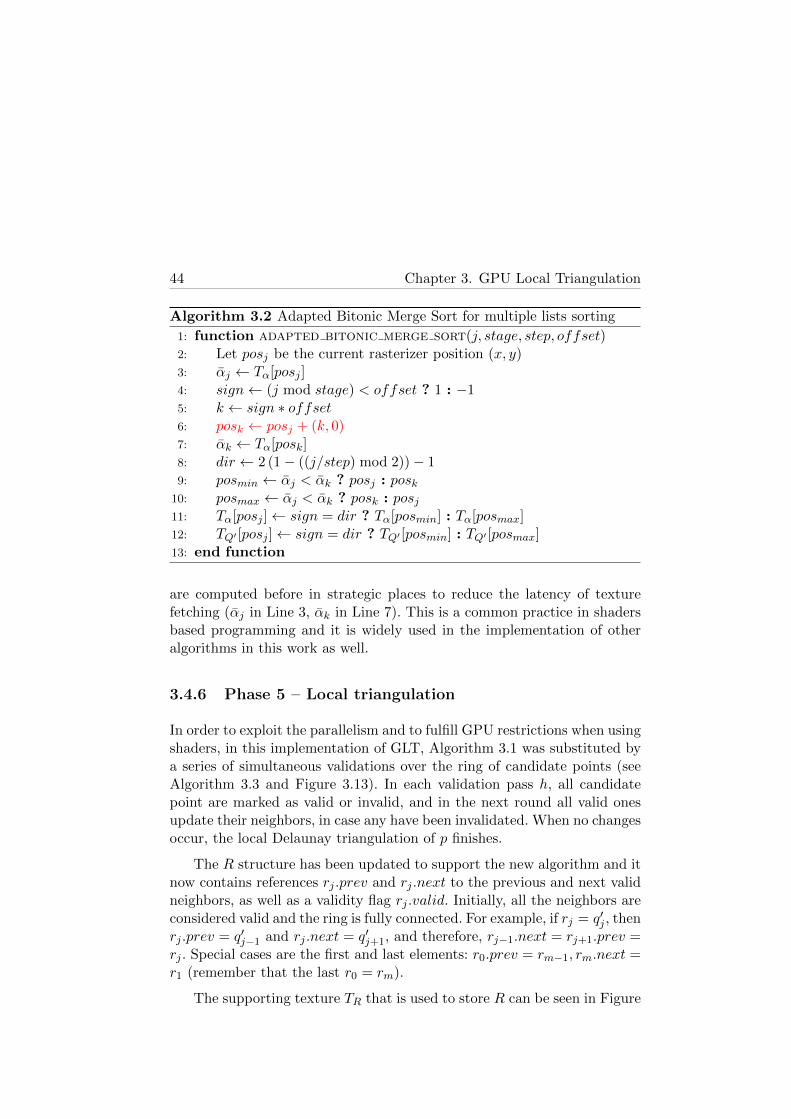
44 Chapter 3. GPU Local Triangulation
Algorithm 3.2 Adapted Bitonic Merge Sort for multiple lists sorting
1: function adapted bitonic merge sort(j, stage, step, offset)2: Let posj be the current rasterizer position (x, y)3: αj ← Tα[posj ]4: sign← (j mod stage) < offset ? 1 : −15: k ← sign ∗ offset6: posk ← posj + (k, 0)7: αk ← Tα[posk]8: dir ← 2 (1− ((j/step) mod 2))− 19: posmin ← αj < αk ? posj : posk
10: posmax ← αj < αk ? posk : posj11: Tα[posj ]← sign = dir ? Tα[posmin] : Tα[posmax]12: TQ′ [posj ]← sign = dir ? TQ′ [posmin] : TQ′ [posmax]13: end function
are computed before in strategic places to reduce the latency of texturefetching (αj in Line 3, αk in Line 7). This is a common practice in shadersbased programming and it is widely used in the implementation of otheralgorithms in this work as well.
3.4.6 Phase 5 – Local triangulation
In order to exploit the parallelism and to fulfill GPU restrictions when usingshaders, in this implementation of GLT, Algorithm 3.1 was substituted bya series of simultaneous validations over the ring of candidate points (seeAlgorithm 3.3 and Figure 3.13). In each validation pass h, all candidatepoint are marked as valid or invalid, and in the next round all valid onesupdate their neighbors, in case any have been invalidated. When no changesoccur, the local Delaunay triangulation of p finishes.
The R structure has been updated to support the new algorithm and itnow contains references rj .prev and rj .next to the previous and next validneighbors, as well as a validity flag rj .valid. Initially, all the neighbors areconsidered valid and the ring is fully connected. For example, if rj = q′j , thenrj .prev = q′j−1 and rj .next = q′j+1, and therefore, rj−1.next = rj+1.prev =rj . Special cases are the first and last elements: r0.prev = rm−1, rm.next =r1 (remember that the last r0 = rm).
The supporting texture TR that is used to store R can be seen in Figure

Section 3.5. Implementation using CUDA 45
3.14. It includes the next and previous valid neighbor in the RG components,the index of the central point (p) and the validity flag in the BA texelcomponents; as all the neighbors of p are stored under the same U coordinate(the same “row”), only the offset from the first neighbor is necessary.
Algorithm 3.3 Local Delaunay triangulation algorithm adaptedfor its implementation with shaders. prev valid neighbor(j) andnext valid neighbor(j) are supporting functions.
1: h← 12: Create T
(0)R from Tα
3: function local 2D Delaunay(j, T(h−1)R ) ⇒ T
(h)R
4: Let posj be the current rasterizer position (x,y)
5: rj ← T(h−1)R [posj ]
6: if rj .valid then7: rj .prev ← prev valid neighbor(j)8: rj .next← next valid neighbor(j)9: rj .valid← is valid(p, q′rj .prev, q
′j , q′rj .next)
10: end if11: return rj12: end function
Finally, this algorithm uses a ping-pong scheme: only two copies of TRare actually used (T
(0)R and T
(1)R ) and in each pass they alternate the reading
and writing roles. This is due to a hardware limitation: texture scatteringis not possible to textures that are being used for fetching.
3.5 Implementation using CUDA
In the previous section numerous adaptations required to implement GLTusing shaders were discussed. Although with the arrival of CUDA manyof these adaptions became unnecessary, not every implementable solutionis efficient (many factors like processors occupancy and accesses to globalmemory have a strong influence in the performance of the CUDA kernel). Inthis section, the main challenges when creating the CUDA implementationwill be discussed. The correspondent algorithm workflow for the CUDAimplementation can be seen in Figure 3.15.

46 Chapter 3. GPU Local Triangulation
Figure 3.13: The shaders implementation of GLT uses a ring tocheck all the neighbors in parallel, discarding the invalid ones ineach iteration.
Figure 3.14: TR – Delaunay ring texture: previous and nextneighbor, the central point and validity flag.
3.5.1 Data structures
In contrast to shaders, CUDA allows the use of more complex datatypessuch as structures, simplifying the design and increasing the data that asingle point may directly store. Even with this advantage, it is convenientto inspect the different algorithms and see what data is actually needed byeach of them. If all the data is stored into a single package, it will increaseunnecessarily the bandwidth required to upload them, as well as reducingthe efficiency of GPU’s cache.
In this sense, instead of dedicating individual sections to each data
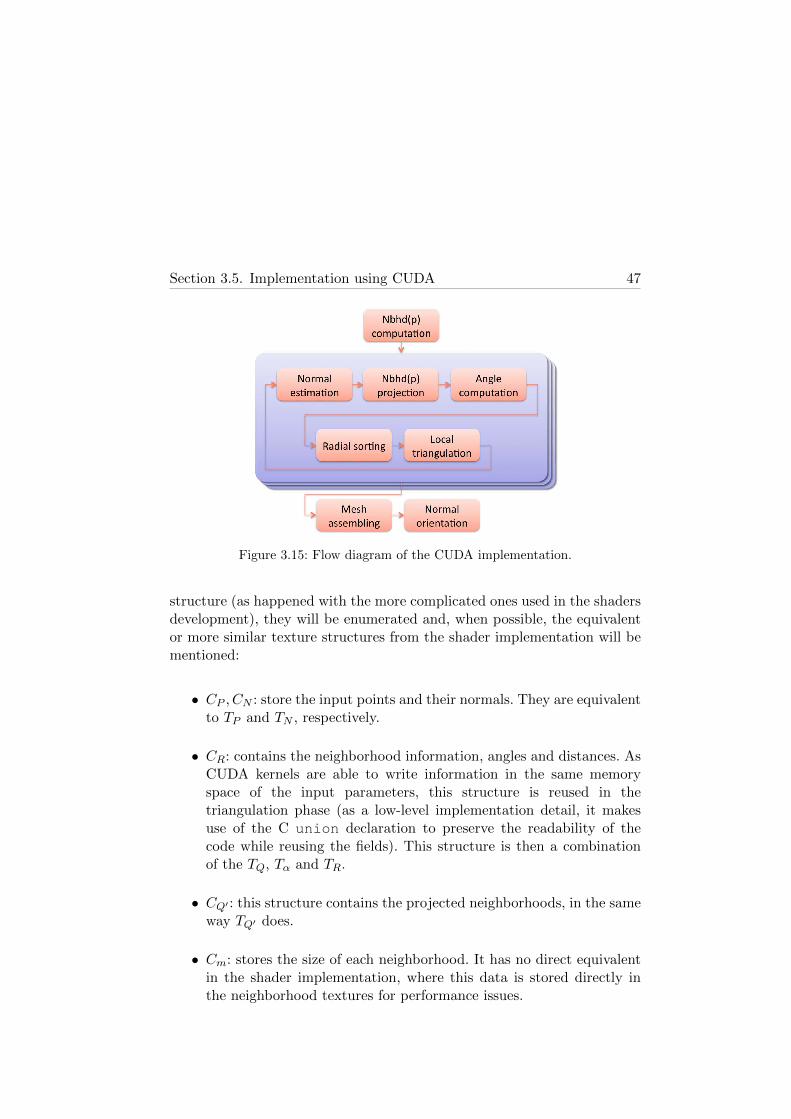
Section 3.5. Implementation using CUDA 47
Figure 3.15: Flow diagram of the CUDA implementation.
structure (as happened with the more complicated ones used in the shadersdevelopment), they will be enumerated and, when possible, the equivalentor more similar texture structures from the shader implementation will bementioned:
• CP , CN : store the input points and their normals. They are equivalentto TP and TN , respectively.
• CR: contains the neighborhood information, angles and distances. AsCUDA kernels are able to write information in the same memoryspace of the input parameters, this structure is reused in thetriangulation phase (as a low-level implementation detail, it makesuse of the C union declaration to preserve the readability of thecode while reusing the fields). This structure is then a combinationof the TQ, Tα and TR.
• CQ′ : this structure contains the projected neighborhoods, in the sameway TQ′ does.
• Cm: stores the size of each neighborhood. It has no direct equivalentin the shader implementation, where this data is stored directly inthe neighborhood textures for performance issues.

48 Chapter 3. GPU Local Triangulation
3.5.2 Phase 4 – Radial sorting
In the shader implementation of GLT, the radial sorting is performed usinga modified version of the Bitonic Merge Sort, optimized to work with severalsmall lists at a time. For the CUDA implementation, three different sortingalgorithms were tested: the modified Bitonic Merge Sort (see Section 3.4.5),Insertion Sort (Knuth, 1998) and the widely known Bubble Sort. Comparingthe times of each one, it could be seen that, even when it has a quadraticcomplexity, the Bubble Sort produced the best results. It is due to the factthat the lists are small, and that the other algorithms use more registers,reducing the occupancy of the GPU.
3.5.3 Phase 5 – Local triangulation
The ring-based algorithm exposed in Section 3.4.6 has been proved to beboth valid (from proof in Section 3.3.7.2) and efficient when implementedwith shaders. But the ping-pong scheme used is no longer needed giventhat CUDA allows the threads to randomly write in any global memoryposition. However, initial tests showed that the GPU occupancy wasvery low using it, decreasing the performance in CUDA. On the otherhand, a direct implementation of Algorithm 3.1 is not possible since itdepends on a dynamic structure to delete the invalid neighbors. Instead,a mixed version has been created using the extended ring structure ofthe shaders implementation and the basis of the iterative backtracking,while introducing a new rj .valid field that replaces the erasing of invalidneighbors.
3.6 Experiments and results
Three versions of the Local Delaunay Triangulation method were tested: theproposed CPU implementation of (Gopi et al., 2000), and the two discussedvariations of GLT: using shaders and using CUDA. Additionally, tests usinganother existing method, the Poisson reconstruction (Kazhdan et al., 2006)are shown.
All tests in this work were performed on several known and publicdatasets, as well as in a few private models. The public models used in this
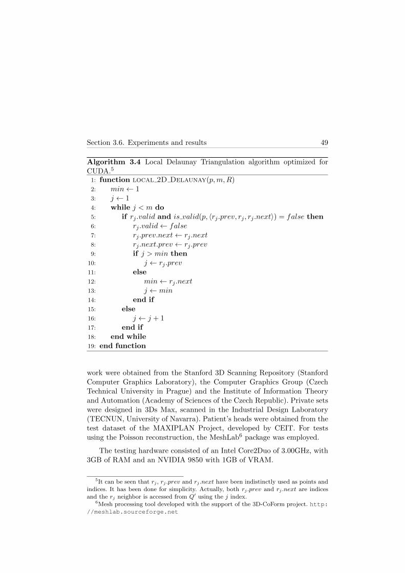
Section 3.6. Experiments and results 49
Algorithm 3.4 Local Delaunay Triangulation algorithm optimized forCUDA.5
1: function local 2D Delaunay(p,m,R)2: min← 13: j ← 14: while j < m do5: if rj .valid and is valid(p, 〈rj .prev, rj , rj .next〉) = false then6: rj .valid← false7: rj .prev.next← rj .next8: rj .next.prev ← rj .prev9: if j > min then
10: j ← rj .prev11: else12: min← rj .next13: j ← min14: end if15: else16: j ← j + 117: end if18: end while19: end function
work were obtained from the Stanford 3D Scanning Repository (StanfordComputer Graphics Laboratory), the Computer Graphics Group (CzechTechnical University in Prague) and the Institute of Information Theoryand Automation (Academy of Sciences of the Czech Republic). Private setswere designed in 3Ds Max, scanned in the Industrial Design Laboratory(TECNUN, University of Navarra). Patient’s heads were obtained from thetest dataset of the MAXIPLAN Project, developed by CEIT. For testsusing the Poisson reconstruction, the MeshLab6 package was employed.
The testing hardware consisted of an Intel Core2Duo of 3.00GHz, with3GB of RAM and an NVIDIA 9850 with 1GB of VRAM.
5It can be seen that rj , rj .prev and rj .next have been indistinctly used as points andindices. It has been done for simplicity. Actually, both rj .prev and rj .next are indicesand the rj neighbor is accessed from Q′ using the j index.
6Mesh processing tool developed with the support of the 3D-CoForm project. http://meshlab.sourceforge.net

50 Chapter 3. GPU Local Triangulation
3.6.1 CPU vs Shaders vs CUDA
Experiments consisted in a comparison of the different GLTimplementations running in the hardware specified above. The setupof the method was 32 points for the neighborhood size and a supportradius similar to the sampling rate of each model (some of them wereobtained empirically since it was not provided).
For each model, ten executions were done and times were averaged.Execution times are shown in Table 3.1 and in the sequence from Figure3.16 to Figure 3.21 a time comparison of each phase using the three GLTimplementations while Figure 3.22 shows total reconstruction times.
Model Size CPU Shaders CUDA
Noisy Foot 20K 1.55s 0.82s 0.44sStanford Bunny 35K 2.81s 1.47s 0.77sHorse 48K 3.65s 1.84s 0.92sRunning Shoe 51K 4.07s 2.06s 1.06sCollar 60K 4.71s 2.41s 1.28sPatient’s Head 1 148K 11.18s 5.82s 3.05sArmadillo 172K 9.59s 6.95s 3.66sAngel 237K 18.62s 10.60s 5.59sEG’07 Dragon 240K 18.45s 9.68s 5.00sPatient’s Head 2 325K 24.46s 13.50s 6.38sHand 327K 24.29s 12.73s 6.39sStanford Dragon 437K 33.64s 17.37s 8.90sHappy Buddha 543K 41.47s 21.46s 11.08sPatient’s Head 3 611K 46.19s 24.68s 13.25sRamorig 622K 46.80s 24.42s 12.54sBlade 882K 69.30s 35.57s 18.37s
Table 3.1: Total reconstruction time using three differentimplementations. In general, Shaders implementation beats upCPU by a factor of 2 while CUDA offers the same boost withrespect to the Shaders. These times are also shown in Figure 3.22.

Section 3.6. Experiments and results 51
Figure 3.16: Time comparison of the computation of theneighborhoods.
Figure 3.17: Time comparison of the normal estimation phase.
Figure 3.18: Time comparison of the angle computation andprojection phase.

52 Chapter 3. GPU Local Triangulation
Figure 3.19: Time comparison of the sorting phase.
Figure 3.20: Time comparison of the local Delaunay validation.
Figure 3.21: Time comparison of the local Delaunay triangulation(validation plus mesh creation).

Section 3.6. Experiments and results 53
Figure 3.22: Comparison between the different proposedreconstruction methods.
3.6.2 Reconstruction results
In this section a few reconstructed models from Table 3.1 are shown. For amore complete list of images, please refer to Section 5.2, where final resultsof this work are exposed. Please, note that all the images in this work wererendered with flat shading to emphasize the actual mesh quality.
Figures 3.23 and 3.24 show the behavior of the GLT under well sampledmeshes (in this case, the model is obtained from a previously reconstructeddataset). Regarding tests of GLT from another sources, Figure 3.25 isthe reconstruction of a synthetic model and Figure 3.26 is from a roughscanning of a shoe.
This last figure shows a hole in the top zone of the model; holes andoverlapping triangles may be generated if four or more points lie on the samecircumference. In such case, the Delaunay triangulation is not unique.
Finally, in Figure 3.27 and Figure 3.28, the Blade model is shown. Thisis the biggest model shown in Table 3.1, with 882954 points. Although abigger model (the Asian Dragon) was reconstructed in these experiments, itwas removed from the graphs due to the difference in the order of magnitudeof the times (its times are shown in Figure 3.29).

54 Chapter 3. GPU Local Triangulation
Figure 3.23: Horse model rendered along with its wireframe.
Figure 3.24: Neck and chest detail of the Horse model.

Section 3.6. Experiments and results 55
Figure 3.25: A synthetic model.
Figure 3.26: Running shoe along with its wireframe. Note that,even when the mesh quality is pretty good, some holes may becreated due to bad sampling as the one visible at the top of theshoe.

56 Chapter 3. GPU Local Triangulation
Figure 3.27: Blade model.
Figure 3.28: Top view of the Blade model. Small structures, asholes, were satisfactorily reconstructed.

Section 3.6. Experiments and results 57
3.6.3 Big models
In this section, reconstruction results for three models with more than amillion points are presented. Figure 3.29 details the time consumption foreach phase during the reconstruction of the Asian Dragon model. Table 3.2summarizes the total reconstruction time of each model using the CUDAimplementation. It is remarkable to say that, even when the Welsh Dragonmodel has more than a million points, it is not quite representative giventhat its points are distributed in a highly uniform way.
Figure 3.29: Overall view of time consumption in thereconstruction of the Asian Dragon model (3609K points). It canbe seen how more than 75% of the time is spent in CPU phases(neighborhoods computation and mesh assembling). Normalpropagation is not shown in this chart. The total reconstructiontime for this model, including the propagation, is 73.25 seconds.
Model Size CUDA Normal propagation
Welsh Dragon 1105K 19.48s 4.92sAsian Dragon 3609K 56.04s 16.15sThai Statue 4999K 78.16s —
Table 3.2: Total reconstruction time of three big models using theCUDA implementation. Due to memory limitations, the normalpropagation of the Thai Statue model was not possible.
Studying the normal propagation in big models, it has been found that

58 Chapter 3. GPU Local Triangulation
the memory consumption is quite significative given the data structuresrequired for it. The Thai Statue model is a good example of it, as it canbe seen in Table 3.2, where the memory employed exceeds the 2GB, thelimit for a single process in the operating system used (Windows XP SP332bits).
3.6.4 Comparison with an approximating method
In addition to the comparison of the presented method, GLT, with theoriginal Lower Dimensional Localized Delaunay triangulation of (Gopiet al., 2000), the Poisson reconstruction (Kazhdan et al., 2006) has beenemployed to reconstruct some of the models previously listed. Table 3.3summarizes these results, and a graphical comparison between GLT andPoisson is shown from Figure 3.30 to Figure 3.33.
Model Size Poisson CUDA GLT
Noisy Foot 20K 4.84s 0.44sAngel 237K 32.38s 5.59sHappy Buddha 543K 58.74s 11.08sBlade 882K 135.66s 18.37sAsian Dragon 3609K 181.82s 73.25s
Table 3.3: Total reconstruction time using the Poissonreconstruction tool from MeshLab. The Noisy Foot, the Bladeand the Asian Dragon employed an octree of depth 10, while theAngel and the Happy Buddha a depth of 9.
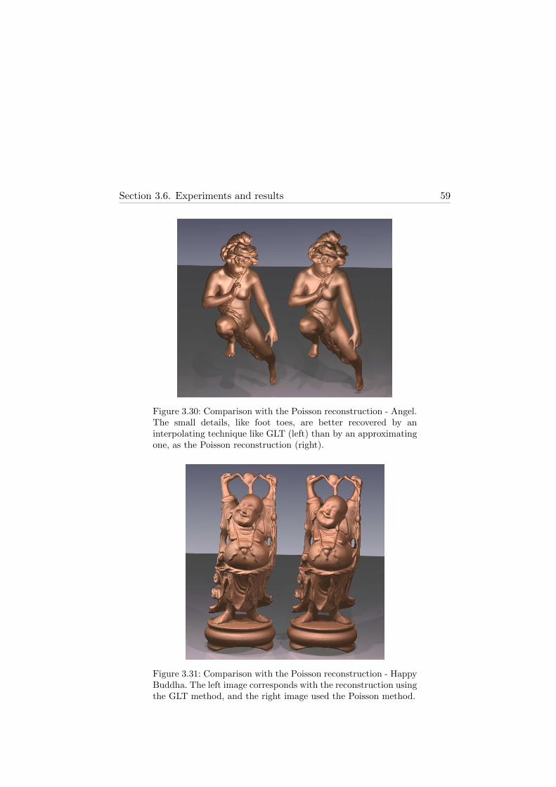
Section 3.6. Experiments and results 59
Figure 3.30: Comparison with the Poisson reconstruction - Angel.The small details, like foot toes, are better recovered by aninterpolating technique like GLT (left) than by an approximatingone, as the Poisson reconstruction (right).
Figure 3.31: Comparison with the Poisson reconstruction - HappyBuddha. The left image corresponds with the reconstruction usingthe GLT method, and the right image used the Poisson method.

60 Chapter 3. GPU Local Triangulation
Figure 3.32: Comparison with the Poisson reconstruction - Blade.The serial number is more readable in the surface generated withthe GLT (left), but the Poisson method (right) is less prone totopological issues like the union of the blade with the base, wheresampling is ambiguous.
Figure 3.33: Comparison with the Poisson reconstruction - Interiordetail of the Blade model. The left image was reconstructedusing the GLT method, and the right image using the Poissonreconstruction.

Section 3.6. Experiments and results 61
3.6.5 Application in the medical field
Figure 3.34 shows the results of the proposed GLT method in the medicalapplication MAXIPLAN (a project developed by CEIT). GLT is used toreconstruct the skin of patients’ heads. The points are extracted from thesegmentation of CT images (computerized tomographies). In this case, theclassical Marching Cubes method is not enough since the mesh shouldbe deformed using a mass-spring model from the segmented points (SanVicente et al., 2009). Using an approximating technique, such as directiso-surface extraction, may create non box-aligned points, a requirement ofthe simulator. Creating a morpher that links the mass-spring model withthe extracted iso-surface would be unnecessarily expensive compared witha direct interpolating reconstruction.
Figure 3.34: From left to right: Patient’s Head 1, Patient’s Head2 and Patient’s Head 3 datasets. As points are extracted from avolumetric source (CT images), the reconstruction presents thisstair-like appearance.
3.6.6 Application in cultural heritage
The models studied in previous sections could be classified into an “objects”category, i.e., models where the scanner goes around the target and it isusually near the scanned object. This is a valid scenario if the target objectis an sculpture, a vase, an anatomical region, and similars; but if the desiredsurface comes from an open area such as a room or a garden, or wherethe scanner is far from the target, like a building, then the reconstruction

62 Chapter 3. GPU Local Triangulation
becomes different since the points cloud tends to be more sparser and it isfar from being uniformly distributed.
This differentiation is necessary before exposing results of thereconstruction method applied to cultural heritage, since it presents datasets of both kinds. This section presents results of applying the proposedmethod to three different models from cultural heritage projects7. Figure3.35, for example, comes from a scanned Trophy, belonging to the “object”type, while the Figure 3.36 is a Roman Theatre, it is, an open space. It canbe seen that GLT fails to properly reconstruct the Theatre model, given thepoints, due to the nature of the scanning process used, have a very unevendistribution, as well as too much missing areas. This sparse and non-uniformstructure makes impossible to determine a satisfactory sampling distance:near the scanner points are very dense while it becomes sparser as it goesaway the centre. Finally, the Tower shown in Figure 3.37 could be properlyreconstructed although it comes from a similar scanning process, becauseit provided four different views of the tower that mutually compensatethe lack of information (these view were aligned as a preprocessing step).Also, this model is more simple than the Theatre, in terms of the samplingdistance, so it is possible to find a maximum value that do not generatefalse positives (points not belonging to the real neighborhood of a point).
Figure 3.35: Reconstruction of a Trophy.
7Models courtesy of Prof. Juan Carlos Torres, University of Granada.

Section 3.6. Experiments and results 63
Figure 3.36: This Theatre has not been succesfully reconstructeddue to the sparseness of the points of the auditorium zone. Onlythe wall could be extracted correctly.
Figure 3.37: Reconstruction of a Tower. The points of the differentviews of the scanner were aligned before the reconstruction.

64 Chapter 3. GPU Local Triangulation
3.7 Discussion
In this chapter, a local Delaunay triangulation for surface reconstructionhas been presented, proving (both mathematically and empirically) thatlocal triangulations are good candidates for parallelization and that they aresuitable for GPU implementation. It has been shown how the proposed GLTmethod can efficiently reconstruct a surface from a set of points, showingan average improvement of two or three times over the state-of-the-artmethods.
Other main contributions of this chapter include changes to the normalestimation phase using Weighted PCA, the improvement of the anglecomputation phase using a modification of the technique proposed by(Crossno and Angel, 1999) and the development of a multi-list sortingalgorithm based on the Bitonic Merge Sort.
Regarding the surface generated, as GLT interpolates the input pointsit depends on their quality. Once the surface has been generated, apost-processing operator such as mesh smoothers can be applied to obtaina softer surface. Also, a preprocessing step can be applied to improve thepoints before the reconstruction.
The withdraws of the method proposed are its dependence to someuniformity in points distribution as well as a proper points density alongzones with higher detail. For example, holes may appear if there are notenough points, or crossing triangles may be created if the density is notenough for the level of detail. Also, it was shown that, although themethod itself can handle large datasets, the normal propagation stage stillrepresents an issue to be solved.
Among the application of studied techniques in other fields, thedivide-and-conquer nature local triangulations makes them appropriate formesh streaming. For example, a model is partitioned using a uniform grid,and each cell or block is sent individually; each block that already has itsneighbors received can be safely reconstructed.

Chapter 4
Parallel Weighted LocallyOptimal Projection
The simplification of anythingis always sensational
Gilbert Chesterton
A synthesis of this chapter has been published in:
Buchart, C., Amundarain, A., and Borro, D. 3-D surface geometryand reconstruction: Developing concepts and applications, chapterHybrid surface reconstruction through points consolidation. IGIGlobal. 2011. (Sent and under revision).
4.1 Previous works
There are some interesting works regarding a preprocess step beforereconstruction. As mentioned before, one of the major problems concerningall the methods is the quality of the input data. What preprocessing stepstry to do is to improve such quality, removing noise and generating a moreuniform set of points. It is especially convenient for interpolating methods,due to their dependence on the input data.
(Alexa et al., 2003) study the direct visualization of point set surfaces,defining a projection operator that projects the points near the data set ontothe surface, and then constructing a moving least-square surface (Levin,2003).
65

66 Chapter 4. Parallel Weighted Locally Optimal Projection
In more recent years, (Lipman et al., 2007b) present aparameterization-free projection operator called LOP (Locally OptimalProjection) to deal with outliers, and (Huang et al., 2009) developed a newWLOP (Weighted LOP), improving the previous operator with a moreuniform distribution of points and a clearer convergence. This operator isalso used to boost up normal estimation and propagation. One of the mainproblems of these operators is that they are very expensive in terms ofexecution time when compared to the time required for the most commonreconstruction algorithms.
Finally, (Zhang et al., 2010) propose a meshless parameterization andde-noising of a set of points by rigid alignment of locally flattered proximitygraphs.
In this chapter, the works of (Lipman et al., 2007b) and (Huang et al.,2009) are studied and a parallel implementation is presented in order toincrease the performance of the operator.
4.1.1 Locally Optimal Projection Operator
Given a set of points P = {pj} , j ∈ J = {1, 2, . . . , |P |}, an initial guessX0 = {xi} , i ∈ I =
{1, 2, . . . ,
∣∣X0∣∣}, a repulsion parameter µ ∈ [0, 1/2)
and support radius h, the Locally Optimal Projection (LOP) algorithmpresented by (Lipman et al., 2007a) computes the projection of X onto Pin an iterative way1. For each iteration k ∈ 1, 2, 3 . . . it defines the projectionfor the i-th point of X:
x(k)i =
∑j∈J
pjα(k−1)ij∑
j∈Jα
(k−1)ij
+ µ
∑i′∈I\{i}
(x
(k−1)i − x(k−1)
i′
)β
(k−1)ii′∑
i′∈I\{i}
β(k−1)ii′
, i ∈ I (4.1)
where
α(k)ij =
θ(∥∥∥x(k)
i − pj∥∥∥)∥∥∥x(k)
i − pj∥∥∥ (4.2)

Section 4.1. Previous works 67
β(k)ii′ =
θ(∥∥∥x(k)
i − x(k)i′
∥∥∥)∥∥∥x(k)i − x
(k)i′
∥∥∥∣∣∣∣∂η∂r (∥∥∥x(k)
i − x(k)i′
∥∥∥)∣∣∣∣ , i′ ∈ I\ {i} (4.3)
θ (r) is a weight function with compact support radius h, that definesthe area of influence of the operator; it can be seen as a Gaussian filter
applied to the distance function from x(k)i . η (r) is a repulsion function that
penalizes points going too close to each other. The support radius h isusually set as h = 4
√dBB/ |P |, where dBB is the diagonal length of the
bounding box of P (Huang et al., 2009). In the work of (Lipman et al.,2007a), such functions are defined as
θ (r) = e−r2/(h/4)2 (4.4)
η (r) =1
3r3(4.5)
4.1.2 Weighted Locally Optimal Projection Operator
In their extension of LOP, (Huang et al., 2009) comment that therepulsion force may decrease too fast in many situations, contributing to anon-uniform distribution of points in X. They then propose a new repulsionterm “which decreases more gently and penalizes more at larger r, yieldingboth a better convergence and a more locally regular point distribution”(Huang et al., 2009, p. 3). They also set, empirically, µ = 0.45. The newrepulsion function is
η (r) = −r (4.6)
which also leads to a simplified β term
β(k)ii′ =
θ(∥∥∥x(k)
i − x(k)i′
∥∥∥)∥∥∥x(k)i − x
(k)i′
∥∥∥ , i′ ∈ I\ {i} (4.7)
1In the whole of this work, ‖ · ‖ represents the Euclidean norm of a vector
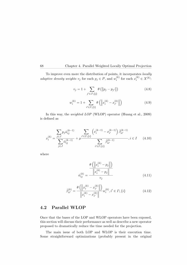
68 Chapter 4. Parallel Weighted Locally Optimal Projection
To improve even more the distribution of points, it incorporates locally
adaptive density weights vj for each pj ∈ P , and w(k)i for each x
(k)i ∈ X(k):
vj = 1 +∑
j′∈J\{j}
θ(∥∥pj − pj′∥∥) (4.8)
w(k)i = 1 +
∑i′∈I\{i}
θ(∥∥∥x(k)
i − x(k)i′
∥∥∥) (4.9)
In this way, the weighted LOP (WLOP) operator (Huang et al., 2009)is defined as
x(k)i =
∑j∈J
pjα(k−1)ij∑
j∈Jα
(k−1)ij
+ µ
∑i′∈I\{i}
(x
(k−1)i − x(k−1)
i′
)β
(k−1)ii′∑
i′∈I\{i}
β(k−1)ii′
, i ∈ I (4.10)
where
α(k)ij =
θ(∥∥∥x(k)
i − pj∥∥∥)∥∥∥x(k)
i − pj∥∥∥
vj(4.11)
β(k)ii′ =
θ(∥∥∥x(k)
i − x(k)i′
∥∥∥)∥∥∥x(k)i − x
(k)i′
∥∥∥ w(k)i , i′ ∈ I\ {i} (4.12)
4.2 Parallel WLOP
Once that the bases of the LOP and WLOP operators have been exposed,this section will discuss their performance as well as describe a new operatorproposed to dramatically reduce the time needed for the projection.
The main issue of both LOP and WLOP is their execution time.Some straightforward optimizations (probably present in the original

Section 4.2. Parallel WLOP 69
implementations, but no details are given in the publications) may includecomputing squared distances instead of the actual distance; and avoidingevaluating the weight function θ(r) on the full domain, but only where itsweight does not vanish, i.e., evaluate the function in the h-vicinity of eachpoint (the main issue with it is the computation of such vicinity).
Even with these optimizations, WLOP is especially slow because it mustevaluate the local density weights in each iteration, which means havingto recompute the h-vicinity of each point several times. In this work, ithas seen that if a good initial guess X0 is provided (see below for furtherexplanation), the neighborhoods variations are small since the points tendto move just a little (weights do change between iterations). The points thatfall into the support of the local density weights of a point have been calledthe local support neighborhood (LSN) of such a point. In this thesis it isproposed to preload an extended LSN that includes all the points that mayfall in the support radius h during the iterations of the operator (see Figure4.1). Even when some neighbors in the extended LSN may fall outside thesupport radius (thus computing unnecessarily the weight function), it isworth the time gained by avoiding the costly neighborhood computation.In tests performed, an extended radius of 2h works well in most of the cases.Also, bounding the maximum number of neighbors is important given thefact that the CUDA matrices are static; in the tests, 64 points of vicinitywere enough to correctly project most of the models, while 128 were usedin noisy models.
Figure 4.1: Local support neighborhood (dark area) vs. theextended LSN (lighter area).
The new local weight densities may be expressed in function of their

70 Chapter 4. Parallel Weighted Locally Optimal Projection
local support neighborhoods as
v(k)j = 1 +
∑j′∈Jj
θ(∥∥pj − pj′∥∥) (4.13)
w(k)i = 1 +
∑i′∈Ii
θ(∥∥∥x(k)
i − x(k)i′
∥∥∥) (4.14)
where Ii defines the precomputed neighborhood of xi, and Jj is the
precomputed neighborhood of pj . To simplify the notation, α(k)ij and β
(k)ii′
will denote the α(k)ij and β
(k)ii′ terms with precomputed neighborhoods.
In the same way, neighborhoods in Equation 4.10 are replaced bytheir precomputed counterparts. Experiments reveal that simply avoidingthe expensive neighborhood computation with the previously exposedtechnique, it is possible to obtain speed up ranges around 50% in theexecution time in the CPU. This variation of the WLOP operator has beencalled extended WLOP, or eWLOP for short.
The only problem so far is the initial guess X0. However, a good andeasy-to-compute initial set can be obtained by the spatial subdivision of P ,taking X0 as the centroid of the points inside each cell. This also followsthe common sense that a uniform data set may be crudely represented bya grid-based subsampling of the point set.
At this point, it raises the question about parallelization. The lessparallel part of the algorithm is neighborhoods computation, but since allthese calculations have been moved to a preprocessing stage, it must bedone just once; the proposed implementation has used the ANN libraryof (Mount and Arya, 2010) to perform the k-nearest neighbors (k-NN)computation2. The rest of the algorithm is data independent in the same
iteration k, i.e., a projected point x(k)i only depends on previously projected
points x(k−1)i′ and the original points P .
Based on the preceding analysis, a Parallel WLOP (PWLOP) thatperforms on average 25 times faster than the original WLOP is proposed.PWLOP uses graphical hardware acceleration by implementing it on theCUDA architecture. It is worth mentioning that, although the algorithm
2When talking about neighborhoods, k is the number of neighbors, not the currentiteration, which is represented between parenthesis: (k).

Section 4.3. Experiments and results 71
is dependent between consecutive iterations, there is no need to doCPU processing after an iteration has finished, so the operator canexecute completely in the GPU before downloads the projected pointsinto the main memory. Additionally, and for testing purposes, the originalWLOP has been modified introducing the extended LSN, but without theparallelization plus of PWLOP (the eWLOP).
4.2.1 Implementation details
The PWLOP operator is susceptible to many optimizations that help tospeed up the method and to reduce the number of GPU registers used,thereby incrementing the GPU occupancy and increasing performance.Some of these optimizations include:
1. Terms like β(k)ii′ , where a norm appears several times; this norm may
be computed only once.
2. Expressions such as
∑j∈J
pjα(k−1)ij∑
j∈Jα
(k−1)ij
can be computed once.
3. The weight function θ (r) = e−r2/(h/4)2 may be expressed as θ (r) =
e−hr2, where h = (4/h)2 is precomputed. Moreover, the distance r
may be used in its squared form, avoiding the costly squared root (inthis sense, for example, many k-NN algorithms return the squareddistances).
4. Finally, there are several terms that may produce a division-by-zerowhen the distance between two points vanishes (more likely betweenX and P ). To solve this issue, and to avoid inconvenient branches,since the divisor is always positive (distances) it is common to add asmall value to it.
4.3 Experiments and results
Figure 4.2 shows a comparison of the execution time of the WLOP, theextended WLOP and PWLOP for a simple model.

72 Chapter 4. Parallel Weighted Locally Optimal Projection
Figure 4.2: Speed comparison between WLOP, eWLOP andPWLOP in the projection of 22K points from the Stanford Bunny(35K points), using a different number of iterations.
In these experiments, the local support neighborhood of the eWLOPand PWLOP was set to 32 points. For WLOP tests and rendering of results,the Points Consolidation API was employed (it is publically available in(Huang et al., 2010)).
Figure 4.3 and Figure 4.4 show projection results for the Happy Buddhamodel. In Figure 4.3, the initial guess is a random subsampling of themodel and the number of iterations is set to 50 for both methods. As theinitial guess is crude, the PWLOP operator fails to converge since the localweight densities were calculated over wrong neighborhoods. On the otherhand, Figure 4.4 shows a more accurate initial guess, extracted from thegrid subdivision described above. As the initial guess is near a solution, thenumber of iterations was reduced to only 10. It can be seen how the resultsfrom WLOP and PWLOP are almost identical, while PWLOP executesfour times faster than WLOP.
As an additional test, the speed comparison seen in Figure 4.4 wasextended to include the eWLOP and increasing the number of iterations.Results can be seen in Table 4.1. It shows how PWLOP can execute 50times more iterations than the original WLOP in the same period of timeunder equal circumstances (the initial guess set). Also, the average speedup offered by PWLOP against the extended WLOP is of 25 times, ignoringthe common neighborhood computation time (6.55s).
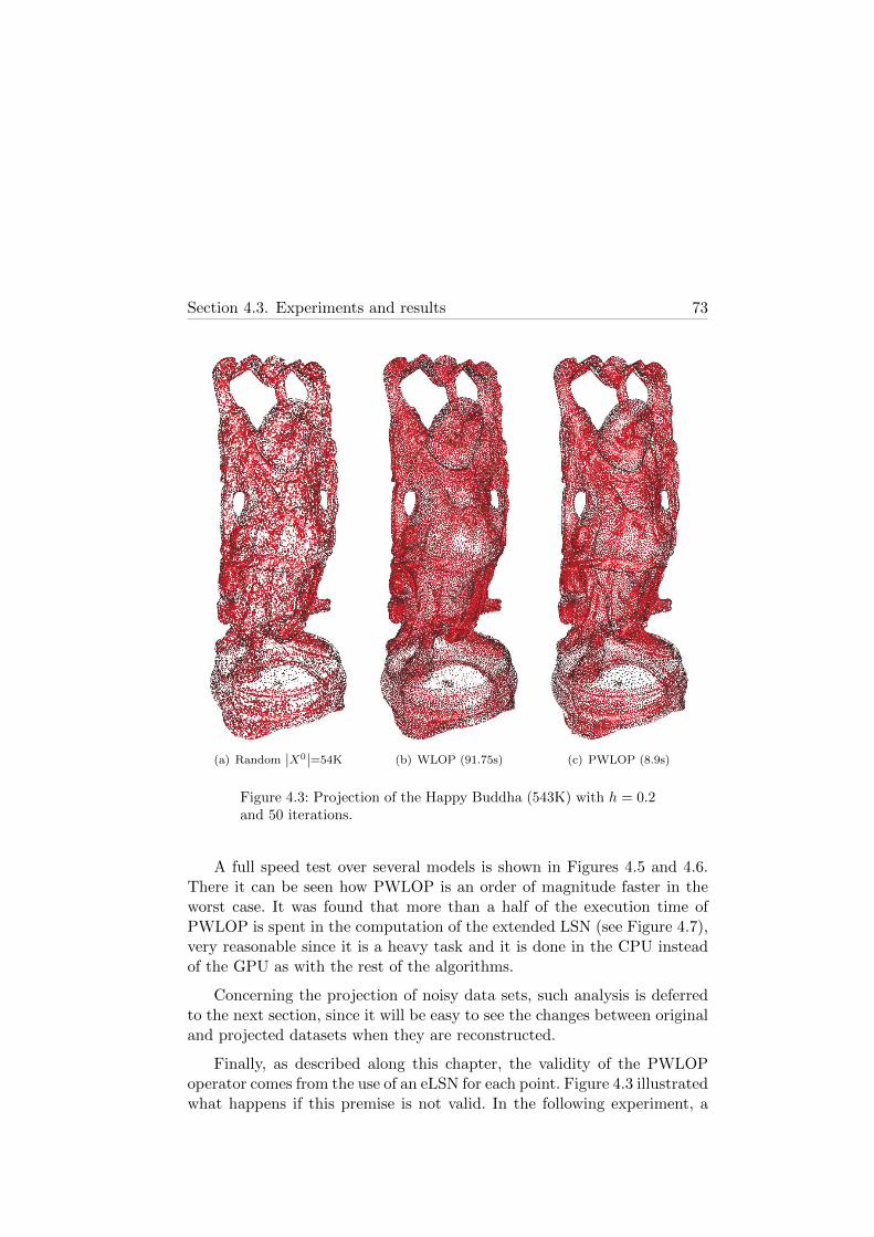
Section 4.3. Experiments and results 73
(a) Random∣∣X0
∣∣=54K (b) WLOP (91.75s) (c) PWLOP (8.9s)
Figure 4.3: Projection of the Happy Buddha (543K) with h = 0.2and 50 iterations.
A full speed test over several models is shown in Figures 4.5 and 4.6.There it can be seen how PWLOP is an order of magnitude faster in theworst case. It was found that more than a half of the execution time ofPWLOP is spent in the computation of the extended LSN (see Figure 4.7),very reasonable since it is a heavy task and it is done in the CPU insteadof the GPU as with the rest of the algorithms.
Concerning the projection of noisy data sets, such analysis is deferredto the next section, since it will be easy to see the changes between originaland projected datasets when they are reconstructed.
Finally, as described along this chapter, the validity of the PWLOPoperator comes from the use of an eLSN for each point. Figure 4.3 illustratedwhat happens if this premise is not valid. In the following experiment, a

74 Chapter 4. Parallel Weighted Locally Optimal Projection
(a) Grid∣∣X0
∣∣=55K (b) WLOP (24.63s) (c) PWLOP (6.87s)
Figure 4.4: Projection of the Happy Buddha (543K) with h = 0.2and 10 iterations.
random set of points is used as the initial set and, instead of using theeLSN and computing it only in the first iteration, the LSN is used forseveral iterations and it is marked to be recomputed each 10 iterations.This leads to a midpoint approach between the original WLOP, thatcomputes the LSN in each iteration, and the PWLOP, that uses only thefirst eLSN. Results of this experiment are shown in Figure 4.8. As can beseen, this approach leads to a slightly better projection than WLOP. Onthe other hand, and as expected, the required time is increased considerablycompared with PWLOP, although it remains inferior to the one employedby WLOP.

Section 4.3. Experiments and results 75
Iterations WLOP eWLOP PWLOP
10 24.63s 14.59s 6.87s100 101.79s 87.53s 9.58s500 963.11s 410.36s 22.69s
Table 4.1: Speed comparison between WLOP, eWLOP andPWLOP when projecting the Happy Buddha model (543K),∣∣X0
∣∣=55K, h = 0.2.
Figure 4.5: Projection of different data sets using WLOP, theeWLOP and the proposed PWLOP operators. For all the datasets, 50 iterations were used as well as LSN = 64.
Figure 4.6: The Extended LSN computation times are commonfor both the eWLOP and PWLOP. The test configuration is thesame of Figure 4.5.

76 Chapter 4. Parallel Weighted Locally Optimal Projection
Figure 4.7: The computation of the extended local supportneighborhood is the same for the eWLOP (left) and PWLOP(right). The speed boost obtained by the parallelization can beseen in this figure. The model is the Asian Dragon (3609K)projected onto 325K points. Parameters are set to 50 iterations,LSN = 64 and h = 0.02.
(a) WLOP (91.75s) (b) PWLOP (8.9s) (c) PWLOP (41.82s)
Figure 4.8: Projection of the Happy Buddha (543K) with h = 0.2and 50 iterations, resetting the initial data set each 10 iterations.

Section 4.4. Discussion 77
4.4 Discussion
In this chapter, a projection operator for points preprocessing, WLOP, thatincludes noise removal and redistribution of input points, is studied, as wellas a new operator, PWLOP, with parallel capabilities is presented. This newoperator has been designed to be implemented in the GPU using CUDA,because WLOP’s limitations made it unsuitable for parallel architectures.PWLOP is an order of magnitude faster than the previous WLOP operator,while keeping the accuracy of the original operator.

78 Chapter 4. Parallel Weighted Locally Optimal Projection

Chapter 5
Hybrid surfacereconstruction: PWLOP +
GLT
–[Luke] I can’t believe it–[Yoda] That is why you fail
A synthesis of this chapter has been published in
Buchart, C., Amundarain, A., and Borro, D. 3-D surface geometryand reconstruction: Developing concepts and applications, chapterHybrid surface reconstruction through points consolidation. IGIGlobal. 2011. (Sent and under revision).
5.1 Improving the input data set through pointsconsolidation
Although the local nature of the method presented makes it very favorableto parallelization, it shares one of the biggest disadvantages of manyreconstructions based on Delaunay triangulations: their sensibility to noiseand outliers. In this sense, the points projection operators presented inSection 4.2 help to solve this issue by creating a more uniform set of points,improving the quality of the reconstruction.
79
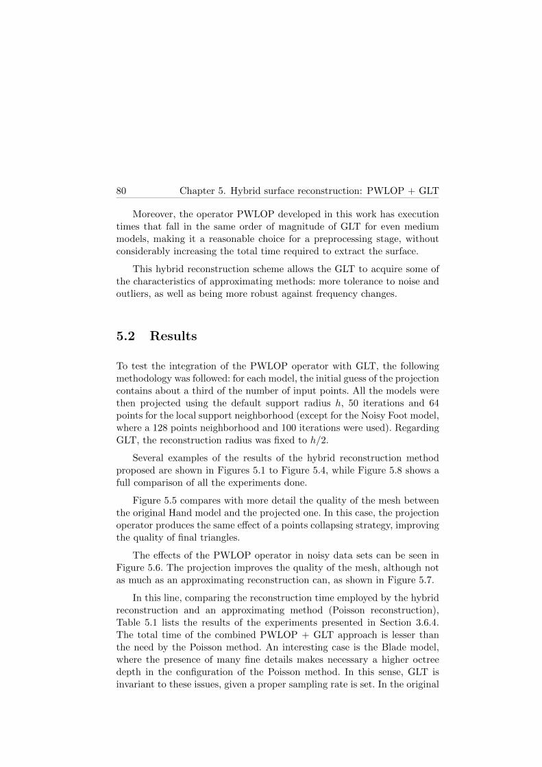
80 Chapter 5. Hybrid surface reconstruction: PWLOP + GLT
Moreover, the operator PWLOP developed in this work has executiontimes that fall in the same order of magnitude of GLT for even mediummodels, making it a reasonable choice for a preprocessing stage, withoutconsiderably increasing the total time required to extract the surface.
This hybrid reconstruction scheme allows the GLT to acquire some ofthe characteristics of approximating methods: more tolerance to noise andoutliers, as well as being more robust against frequency changes.
5.2 Results
To test the integration of the PWLOP operator with GLT, the followingmethodology was followed: for each model, the initial guess of the projectioncontains about a third of the number of input points. All the models werethen projected using the default support radius h, 50 iterations and 64points for the local support neighborhood (except for the Noisy Foot model,where a 128 points neighborhood and 100 iterations were used). RegardingGLT, the reconstruction radius was fixed to h/2.
Several examples of the results of the hybrid reconstruction methodproposed are shown in Figures 5.1 to Figure 5.4, while Figure 5.8 shows afull comparison of all the experiments done.
Figure 5.5 compares with more detail the quality of the mesh betweenthe original Hand model and the projected one. In this case, the projectionoperator produces the same effect of a points collapsing strategy, improvingthe quality of final triangles.
The effects of the PWLOP operator in noisy data sets can be seen inFigure 5.6. The projection improves the quality of the mesh, although notas much as an approximating reconstruction can, as shown in Figure 5.7.
In this line, comparing the reconstruction time employed by the hybridreconstruction and an approximating method (Poisson reconstruction),Table 5.1 lists the results of the experiments presented in Section 3.6.4.The total time of the combined PWLOP + GLT approach is lesser thanthe need by the Poisson method. An interesting case is the Blade model,where the presence of many fine details makes necessary a higher octreedepth in the configuration of the Poisson method. In this sense, GLT isinvariant to these issues, given a proper sampling rate is set. In the original

Section 5.2. Results 81
work of (Huang et al., 2009), Poisson reconstruction is also improved usinga consolidation of points based on the WLOP operator; so, regarding thereconstruction time, it is also increased in a similar proportion, but, inanyway, the PWLOP operator presented in this work has demonstrated tobe much faster than WLOP, so it can be also used for those cases whereGLT fails to create a proper mesh (for example, very highly clouds of points,or if a watertight surface is needed).
Figure 5.1: Stanford Dragon.

82 Chapter 5. Hybrid surface reconstruction: PWLOP + GLT
Figure 5.2: Asian Dragon.
Figure 5.3: Happy Buddha.
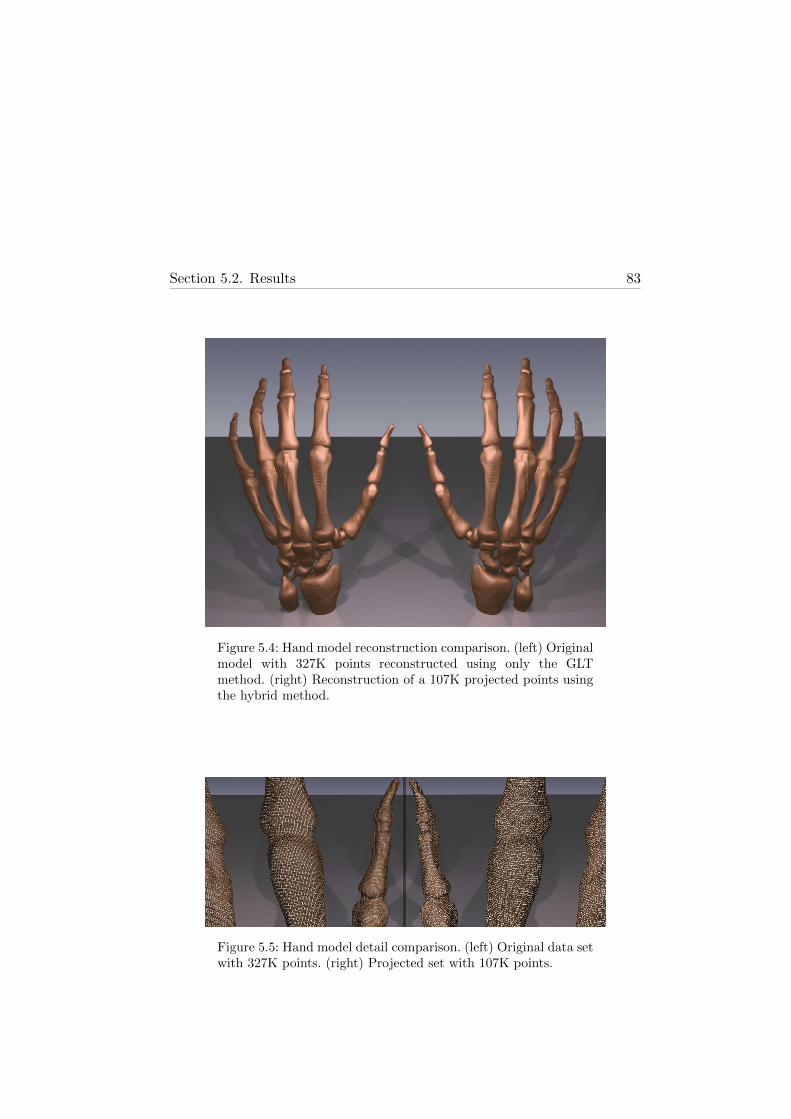
Section 5.2. Results 83
Figure 5.4: Hand model reconstruction comparison. (left) Originalmodel with 327K points reconstructed using only the GLTmethod. (right) Reconstruction of a 107K projected points usingthe hybrid method.
Figure 5.5: Hand model detail comparison. (left) Original data setwith 327K points. (right) Projected set with 107K points.

84 Chapter 5. Hybrid surface reconstruction: PWLOP + GLT
Figure 5.6: Noisy Foot with 20K points. From left toright: original data set; self-projected using PWLOP withLSN=64; self-projected using PWLOP with LSN=128. Biggerneighborhoods are necessary because in noisy data sets the pointsmove more between iterations. It can be seen how the nails are stillrecognizable. For all the images the number of PWLOP iterationswas set to 100.
Model SizeProjected
Poisson HybridSize (Hybrid)
Angel 237K 86K 32.38s 11.73sHappy Buddha 543K 192K 58.74s 25.63sBlade 882K 139K 135.66s 22.97sAsian Dragon 3609K 325K 181.82s 75.89s
Table 5.1: Comparison of reconstruction times between thePoisson method and the proposed hybrid approach. Theintroduction of the PWLOP operator improves the final meshquality, and also reduces the number of points employed in thereconstruction. The size of the projected sets has been chosen totry to match the resolution of Poisson’s results.

Section 5.2. Results 85
Figure 5.7: Noisy Foot with 20K points: (left) using PWLOP +GLT, 1.52s, (right) using the Poisson reconstruction, 4.84s. Itcan be seen how, even when the projection operator improvesthe quality of the mesh, the continuum origin of approximatingapproaches results in softer meshes.

86 Chapter 5. Hybrid surface reconstruction: PWLOP + GLT
Figure 5.8: Results of the hybrid PWLOP + GLT reconstruction.

Section 5.3. Discussion 87
5.3 Discussion
Points set preprocessing is a useful tool if an interpolating reconstructiontechnique is going to be used, in order to reduce the noise of the data, toincrease the quality of the reconstructed mesh and, in some cases, to reducethe size of the input set.
The projection operator PWLOP studied in the previous chaptercreates an uniform set of points that approximates the input data. Inthis chapter, the operator is used as a preprocessing phase to clean upthe points set and to increase its uniformity. Experiments showed that thereconstructed mesh from this hybrid approach presents a higher trianglequality as well as that the reconstruction time is reduced.
A direct application of the hybrid PWLOP + GLT method is in thecreation of multi-resolution meshes; several meshes can be reconstructedby varying the size of the initial points set of PWLOP. A quick example ofthis application can be seen in Figure 5.9.

88 Chapter 5. Hybrid surface reconstruction: PWLOP + GLT
Figure 5.9: Reconstruction of the Happy Buddha in multipleresolution using the hybrid PWLOP + GLT approach. Notethat the first model is too coarse that it no longer satisfies thesampling condition and points near corners are misinterpreted.The approximate resolutions of each model are, from left to right,10K, 26K, 118K, 198K and 396K triangles.

Chapter 6
Study of multi-balloonsreconstruction
If debugging is the process of removing bugs,then programming must be the process of putting them in
Edsger Dijsktra
This chapter studies the possibility of using dynamic techniques for surfacereconstruction, designing a parallel paradigm in order to improve therecovery of global properties of the model.
6.1 Dynamic techniques
Techniques studied in previous chapters are also known as static techniquesbecause they directly reconstruct the target surface. There is another group,known as dynamic techniques, which consist of deformable models thatadjust the destination surface by minimizing an energy function associatedwith the model (such minimization is usually performed in an iterative way,given the non-linear nature of most of these functions)1.
Dynamic methods have been widely used in the segmentation of medicalimages. For example, (Kass et al., 1987) formulate the snakes or deformablecontours, one of the most commonly employed techniques. Snakes areparametric curves that move under the influence of internal forces (defined
1Observe that dynamic techniques may be classified also within the approximatingcategory (Section 2.2), if the construction of the surface is not taken into account.
89

90 Chapter 6. Study of multi-balloons reconstruction
by the curve) and external forces (derived from the image data). Severalworks proposed different formulations for the internal and external forces,but one of the most relevant is the Gradient Vector Flow (Xu and Prince,1998), which is a mixed balance force that points toward the objectboundary near the boundary, but that varies smoothly in homogeneousregions, allowing a better shape recovering as well as forcing the snake toenter into concave zones. Also worth mentioning is the T-Snake (McInerneyand Terzopoulos, 1999), a topology aware snake that is defined in terms ofaffine cell image decomposition2.
Following the idea of snakes, balloons reconstruct a surface representedby a distance function (Miller et al., 1991; Duan and Qin, 2001). In general,balloons consist in subdivision surfaces that evolve to extract the shapeof the 0-valued distance, i.e., they can be seen as the 3D extension ofthe snakes. Balloons can also reconstruct the topology of the model ina natural way; for example, when two evolving components of the balloonare in collision it is possible to merge the surfaces, increasing the genusof the model. In this line, the work of (Sharf et al., 2006) is especiallygood, presenting a competing scheme where active parts of the balloon,called fronts, are inflated by priority according to their relative size. Inthis way, a more intuitive interpretation of data is obtained (Figure 6.1).Along with the definition of balloons, (Duan, 2003) mention the possibilityof using multiple seeds in parallel to improve the reconstruction time. Also,another 3D reconstruction scheme from point clouds is the use of discretemembranes (a connected region of voxels) to recover the shape and topologyof the voxelized point set (Esteve et al., 2005). In a more specific scenario,(Li et al., 2010) present a reconstruction method for arterial objects basedon that those models are basically 1D; from this fact, the method evolvestubular snakes along the skeleton of the scanned models.
Finally, the use of the level set method (Osher and Sethian, 1988) iswidely used in the field of surface reconstruction. Contrary to active contourapproaches like snakes and balloons, the level set method manipulatesthe surface indirectly. The contour (a curve or surface, depending on thedimension) is embedded as the zero level set of a higher dimensionalfunction, which is evolved under the control of a differential equation
2Affine cell image decomposition is a partitioning scheme, very similar to atriangulation, where the space is divided in cells defined by simplices, and cell vertices areclassified as interior, exterior or boundary, depending on their relation with an automaticstructure (the snake in this context).

Section 6.1. Dynamic techniques 91
Figure 6.1: Competing fronts reconstruct in a more intuitive waythe shape and topology of the data (image from (Sharf et al.,2006)).
(Ibanez et al., 2005). The evolution of the contour will vary dependingon the formulation of the level-set function. Its main advantages are thatcomplex shapes can be arbitrarily modeled and topology is easily handled.As an example, (Zhao et al., 2001) formulate the level-set function as asurface energy equivalent to the surface area weighted by some power ofthe distance function. For a full review of the level set method, please referto (Sethian, 1999).
Figure 6.2: Illustration of level sets (image from (Ibanez et al.,2005)).
6.1.1 Classic balloons
In this section, the definition of Competing Fronts (Sharf et al., 2006) andthe Intelligent Balloon (Duan and Qin, 2001) are presented. In a generalway, a balloon is a subdivision surface S that evolves from an arbitraryseed (usually a genus-0 triangle mesh, e.g., a sphere) to minimize an energyfunction over the surface domain Γ like:

92 Chapter 6. Study of multi-balloons reconstruction
E(x) =∑k
ω(k)
∫ΓE(k)(x) (6.1)
where E(k) is a set of forces that regulate the evolution of the balloon, andω(k) is the correspondent weights. Such terms are usually classified intoexternal forces (e.g., attraction to the target surface) and internal forces(such as curvature or tension constrains).
When the subdivision surface is a polygonal mesh, the minimization ofthe function showed in Equation 6.1 can be expressed as:
minE(x) = min∑i
∥∥∥∥∥∑k
ω(k)Ei(k)
∥∥∥∥∥2
(6.2)
where Ei(k) is the k-th force term of the i-th vertex. The forces usedby the Intelligent Balloon include a deformation potential, a boundaryconstraint, a curvature constraint and an angular constraint. In the case ofthe Competing Fronts, these terms are an attraction force (similar to thedeformation potential) and a tension term. The forces used in this work arebetter explained in a subsequent section.
Both Intelligent Balloon and Competing Fronts work similarly. Givena target surface S, they evolve a triangle mesh S, minimizing the distancebetween S and S. This evolution is done by moving the vertices of S inthe outward normal direction toward S. When a vertex reaches a localminimum of the distance function to S it stops moving. This eventuallycreates unconnected mesh components of S (fronts). When the deformablemodel completely stops, the method checks if there are remaining partsof S that have not been satisfied yet. In that case, S is locally refinedto allow the vertices to move towards the target surface. The quality ofthe mesh is guaranteed by interleaving deformation and mesh optimizationoperators. Finally, topology can be changed by merging colliding fronts,which increases the genus of the model by one; the nature of balloons makeshole filling an implicit feature of these methods, so hole recovering must bedone in a post-processing task. Finally, if unconnected structures have tobe reconstructed, additional balloons must be included.
In the case of the Competing Fronts, each front is assigned a tensionfactor that controls the evolution of the front. This control creates acompetition among fronts, allowing bigger fronts, i.e., those with more

Section 6.2. Multi-balloons 93
tension, to evolve faster than small ones. In this way, it recovers the shapeof the model in a coarse-to-fine manner.
6.2 Multi-balloons
One of the main advantages of dynamic techniques is that they providetools to better control the reconstruction of the dataset. For example, inthe reconstruction of a soft tissue from medical images, specific conditionsmay be easily included into an active contours formulation to respondto additional data from MRI (magnetic resonance imaging) for bettercontrast. Another example is the topology control: when two zones of aballoon collide, they are usually stopped to avoid a self-crossing of thesurface. These regions can be merged to increase the genus of the model byone.
In general, and summarizing the previous exposition, balloons performthe reconstruction based on a single deformable surface that is inflated andsubdivided as needed, merging confronting components if required by thetopology of the model.
There are several shape configurations that deserve attention, forexample, long tubular models and objects with several wide zones connectedby small tunnels as well as the previously mentioned models with severalunconnected regions. In these cases, although active contours can correctlyreconstruct the model, they may incur in unnecessary refinements to satisfyfrequent changes in the level of detail.
Inspired in the competing fronts reconstruction (Sharf et al., 2006) andthe multiple seed extension mentioned by (Duan, 2003), a multi-balloonscheme is studied in this section. The idea is to place several independentballoons in each “cave” and let them evolve in parallel. Using multipleballoons not only may improve the performance of the reconstruction,but it concurrently creates a more natural and intuitive reconstructionworkflow, where coarser areas are reconstructed first, refining only thoseparts of the model that have not been fulfilled yet. As mentioned before, thiscoarse-to-fine mechanism brings to mind that used by (Sharf et al., 2006),although in this case it would be possible to actually complete the coarserparts of the model before intruding in narrow zones, thereby recoveringin a more satisfactory way global properties from the data set and also

94 Chapter 6. Study of multi-balloons reconstruction
reducing the number of times that the distance function has to be refined.An overview of the designed algorithm is shown in Algorithm 6.1, whileFigure 6.3 shows a graphical representation of its workflow.
Algorithm 6.1 Overview of the algorithm proposed.
1: Compute distance (F ) and satisfaction (G) fields2: while not reconstructed do3: while level is not finished do4: for each active balloon Bi do5: Inflate(Bi)6: end for7: Detect and solve collisions8: Increase genus if desired9: end while
10: Refine distance function11: end while
Figure 6.3: Flow diagram of the studied reconstruction usingmultiballoon.
In general, the proposal starts with the computation of an unsigneddistance field to the input points that will guide the reconstruction. Multipleseeds are placed inside the model, that will reconstruct coarser regions ofthe model first, with an independent balloon evolving and adjusting inside

Section 6.2. Multi-balloons 95
of each one. When all these regions are satisfied, finer details and unfinishedregions are recovered by refining the distance field, and therefore increasingthe resolution of balloons. In the meantime, collisions are detected to avoidballoon intrusions, and topology changes are tracked. This process continuesuntil all the data set is reconstructed.
Although the method works positioning the seed of each balloon in anyplace, it is more efficient to use one balloon for each region of the model;of course, it is a must to place seeds in each unconnected region. Thosezones may be defined in several ways, for example: not connected cells ofa discrete distance field, a very long tube-like model divided so severalballoons start at different points as proposed by (Li et al., 2010), etc. Foran illustrative example of seed positioning, please see Figure 6.4.
Figure 6.4: Illustrative representation of multiple seeds for theHand model.
The following sections are organized as follows: Section 6.2.1 explainsthe unsigned distance function and the spatial subdivision structure used asa helper, and Section 6.2.2 exposes the evolution process, its concepts anddifferent phases. Section 6.2.3 studies the topology control scheme used inthis work. Finally, Section 6.3 shows some experiments and results of thisproposal.
6.2.1 Scalar function fields
Although not fully introduced yet, this section explains the use andcomputation of the distance function field (F ) and the satisfaction function

96 Chapter 6. Study of multi-balloons reconstruction
field (G) that guides the evolution of the balloons. F serves as an attractionforce for balloons as mentioned before. G, on the other hand, is more widelyused: for tracking the position of inactive regions in collision detection, todetermine which parts of the model have not been reconstructed yet, andto set the mesh resolution. For the definition of F , a kd-tree is used tocompute the nearest point to a vertex, while for G, a multi-resolution 3Dgrid is employed where its voxels are tagged to reflect the position of theballoons.
Concerning performance, it has been seen that for data sets inferior to amillion points, kd-tree queries are nearly as fast as a grid, but considerablymore accurate and the data structure requires less memory3. But even usinga kd-tree for the distance function itself, an underlining grid structure isstill necessary to store information about satisfied regions and to guide theresolution of the mesh.
For most of the models, a few levels of refinement are needed for aproper reconstruction; so a multi-resolution grid, similar to a n-tree4, wasused instead of the more classical octree, preferring fewer levels of depthin the tree rather than a high partitioning of the space. This structure isvery similar to a scalar field with fixed resolution, but each cell of the gridcan be refined to better adapt the level-set zero of the distance function(see Figure 6.5). Although multiple resolutions are possible in each cell andin any level, experiments showed that it is simpler to have a few levels ofrefinement (2 or 3). The resolution of the first level is imposed by the model(so the coarser regions are recovered easily), while following levels partitionthe previous one in 23 (like an octree), 33 or 43 sub-levels. As an exampleof the distance function, please see Figure 6.6.
6.2.2 Evolution process
6.2.2.1 Global and local fronts
Both Competing Fronts and Intelligent Balloon make use local fronts todefine active areas of the balloon, i.e., zones that are not near enough to
3Approximating Nearest Neighbors, (Mount and Arya, 2010), has been used to speedup the queries, setting up an error of a fraction of the cell’s size.
4n-trees are the generalization of binary trees, quadtrees and octrees. Each node ofthe tree may either have no children, or have n subnodes.

Section 6.2. Multi-balloons 97
Figure 6.5: Multi-resolution grid used as satisfaction function.
Figure 6.6: Slice of the Horse model’s distance function.
the target surface. These active fronts are those that are evolved, reducingthe size of the minimization problem.
The creation of the fronts may face several questions: is any activeregion of the balloon considered a front? is there a minimum front size? Itis important because very small fronts (with respect to the precision of thedistance function) may create an ill-posed system, or produce pledges.
Another issue is the tracking of vertices along successive remeshingoperators (refinements, smoothing, etc.). Such operations destroy andcreate vertices, and may change the index scheme of the vertices as wellas new fronts, or may join existing ones. Tracking the vertices of a front is

98 Chapter 6. Study of multi-balloons reconstruction
costly in terms of memory and speed. On the other hand, creating frontsis a fast operation in comparison to the complexity introduced by verticestracking structures, so in this work fronts are computed on-the-fly whenrequired. This fronts are used only to speed up collision detection and todetermine regions to be joined in genus changes. As fronts are not used inthe evolution process, then they must be, at least, as large as the size oftunnels and connecting regions in the target model.
In contrast to previous works, the balloons used in this work employ aglobal front structure, i.e., the whole balloon is taken into account in theevolution. This approach improves the overall quality of the mesh althoughthe evolution speed is reduced. The next section describes a solution to thisproblem.
6.2.2.2 Two-step evolution
In previous works, only active fronts (S components that are not nearenough to S) are included in the evolution of the balloon. In this newformulation, a different approach is studied, evolving the whole balloon ateach step, but weighing the vertices movement depending on their distanceto S (nearer vertices vary less than further parts). In this way, as the wholeballoon is used, it better recovers the open region where it is evolving, andit implicitly generates a coarse-to-fine shape recovering.
In order to reduce the computational requirements of the evolutionof the balloon, the minimization system has been replaced by a two-stepinflation process, where external and internal forces are independentlyapplied.
In the first step, described in Equation 6.3, vertices are moved in thenormal direction toward the target surface, guided by the distance field5.
x(k+1)i = x
(k)i + rin
(k)i
ri = κiF (x(k)i )
(6.3)
The κi is a new modulation term that regulates the attraction force;it will be explained in Section 6.2.2.3. Using a different formulation from
5From now on, k does not refer to a force but to an iteration of the evolution process.

Section 6.2. Multi-balloons 99
the one proposed in previous works, the system is expressed in terms of the
relative displacement ri from x(k)i , rather than the position of the vertex
itself. This point of view comes from a first implementation of the evolutionbased on a minimization system. Using ri provides a twofold advantage:the number of variables that govern the method is reduced, and ri is scaleindependent, which means that minimization methods based on gradientdescent do not have to deal with the absolute size of the model. When themethod was changed to avoid the minimization system, the use of a relativedisplacement remained useful for a faster and easier computation.
In the second step (Equation 6.4), internal forces smooth the surfaceand reduce the tension on it.
Eit =
∑vj∈N
(x(k+1)i
) cij(x
(k+1)i − vj
)∑
vj∈N(x(k+1)i
) cij
cij = cot(αij) + cot(βij)
(6.4)
The tension term Eit , is the Laplace-Beltrami operator over theneighborhood of each vertex xi of the front (Meyer et al., 2002). This isbasically a smoothing operator that is applied to the balloon after eachiteration.
In order to guarantee that the balloons do not penetrate each other,the method detects collisions among the destinationvertices (the verticesof the next k+ 1 iteration) before the evolution phase. As is usual in theseproblems, the intersection between the bounding boxes of the destinationfronts is checked to speed up the detection. The vertices of the intersectingtriangles are removed from the evolution by not allowing them to move,
i.e., x(k+1)i = x
(k)i .
6.2.2.3 Gradient modulation term: κi
To prevent the balloon from being excessively attracted if it is filling a hole,and therefore going away the target surface, a new gradient modulationterm (κi) is introduced into the evolution process. This term is proportional
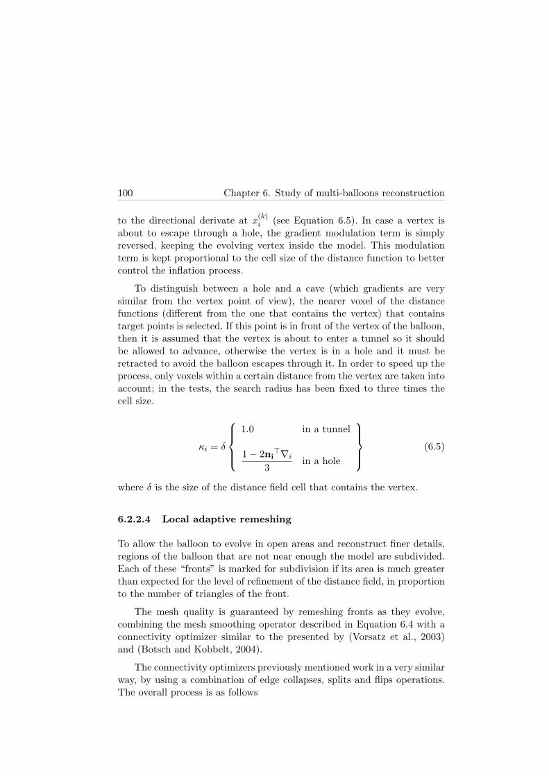
100 Chapter 6. Study of multi-balloons reconstruction
to the directional derivate at x(k)i (see Equation 6.5). In case a vertex is
about to escape through a hole, the gradient modulation term is simplyreversed, keeping the evolving vertex inside the model. This modulationterm is kept proportional to the cell size of the distance function to bettercontrol the inflation process.
To distinguish between a hole and a cave (which gradients are verysimilar from the vertex point of view), the nearer voxel of the distancefunctions (different from the one that contains the vertex) that containstarget points is selected. If this point is in front of the vertex of the balloon,then it is assumed that the vertex is about to enter a tunnel so it shouldbe allowed to advance, otherwise the vertex is in a hole and it must beretracted to avoid the balloon escapes through it. In order to speed up theprocess, only voxels within a certain distance from the vertex are taken intoaccount; in the tests, the search radius has been fixed to three times thecell size.
κi = δ
1.0 in a tunnel
1− 2ni>∇i
3in a hole
(6.5)
where δ is the size of the distance field cell that contains the vertex.
6.2.2.4 Local adaptive remeshing
To allow the balloon to evolve in open areas and reconstruct finer details,regions of the balloon that are not near enough the model are subdivided.Each of these “fronts” is marked for subdivision if its area is much greaterthan expected for the level of refinement of the distance field, in proportionto the number of triangles of the front.
The mesh quality is guaranteed by remeshing fronts as they evolve,combining the mesh smoothing operator described in Equation 6.4 with aconnectivity optimizer similar to the presented by (Vorsatz et al., 2003)and (Botsch and Kobbelt, 2004).
The connectivity optimizers previously mentioned work in a very similarway, by using a combination of edge collapses, splits and flips operations.The overall process is as follows

Section 6.2. Multi-balloons 101
• An edge is split if it is larger than εmaxµ.
• An edge is collapsed if it is shorter than εminµ.
• An edge is flipped if it reduces the valence excess of the neighboringtriangles.
where µ is the objective edge length, satisfying that εmax > 2εmin (Vorsatzet al., 2003). Concerning the values of these terms, (Botsch and Kobbelt,2004) deduced that they should be set to εmax = 4
3 and εmin = 45 , although
it does not satisfy the (Vorsatz et al., 2003)’s proportion. In this work, andin order to fulfill additional requirements, different values were used, as itwill be explained bellow.
Regarding the edge splits and collapses, when the original remeshingoperator is applied, the mesh resolution changes imposed by the hierarchicaldistance field are lost, since the operator tends to create an uniform mesh.In this work, a reduction of the mesh resolution (edge collapse) avoidsrecovering fine details while augmenting the resolution means larger systemsto be solved as well as to allow the balloon to grow through holes. On theother hand, an increment of the resolution (by edge splitting) in very wideareas reduces the stability of the system.
In order to overpass these limitations, the following modification isproposed: instead of being εmin and εmax the minimum and maximumedge lengths, they have slightly different meanings: they represent theminimum and maximum scaling factors for the average edge length ofthe neighborhood of each edge. For stability purposes, the objective edgelength µ has been set to the minimum cell’s size of the distance function,so µ = δmin; this guarantees that almost degenerated triangles do notaffect the overall mesh resolution . The value of both εmin and εmax werealso relaxed in order to allow a softer resolution change in the mesh afterseveral consecutive iterations of the method. It was found that εmin = 3
5 andεmax = 11
6 works well for most of the models. The proposed local adaptiveremeshing operator is listed in Algorithm 6.2 and a comparison betweenit and the uniform remeshing (Vorsatz et al., 2003; Botsch and Kobbelt,2004) is shown in Figure 6.7, while Figure 6.8 shows another example ofthe effects of the new operator.
The optimization of the valence of each vertex makes that most of thevertices have a valence of six. For two neighboring triangles 4 (a, b, c) and
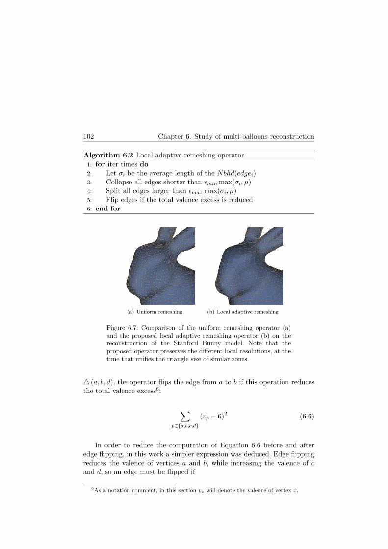
102 Chapter 6. Study of multi-balloons reconstruction
Algorithm 6.2 Local adaptive remeshing operator
1: for iter times do2: Let σi be the average length of the Nbhd(edgei)3: Collapse all edges shorter than εmin max(σi, µ)4: Split all edges larger than εmax max(σi, µ)5: Flip edges if the total valence excess is reduced6: end for
(a) Uniform remeshing (b) Local adaptive remeshing
Figure 6.7: Comparison of the uniform remeshing operator (a)and the proposed local adaptive remeshing operator (b) on thereconstruction of the Stanford Bunny model. Note that theproposed operator preserves the different local resolutions, at thetime that unifies the triangle size of similar zones.
4 (a, b, d), the operator flips the edge from a to b if this operation reducesthe total valence excess6:
∑p∈{a,b,c,d}
(vp − 6)2 (6.6)
In order to reduce the computation of Equation 6.6 before and afteredge flipping, in this work a simpler expression was deduced. Edge flippingreduces the valence of vertices a and b, while increasing the valence of cand d, so an edge must be flipped if
6As a notation comment, in this section vx will denote the valence of vertex x.

Section 6.2. Multi-balloons 103
Figure 6.8: Detail of the effects of the local adaptive remeshingoperator proposed in this work. Note that the resolution changessmoothly through the mesh thanks to the new average objectiveedge length.
∑p∈{a,b,c,d}
(vp − 6)2 > (va − 1− 6)2 + (vb − 1− 6)2
+(vc + 1− 6)2 + (vd + 1− 6)2
(6.7)
Expanding out each expression of Equation 6.7, rearranging the termsand simplifying leads to the simpler condition
va + vb > 2 + vc + vd (6.8)
At the end of the evolution process, fine details may have not beenreconstructed yet due to the resolution of the mesh near the features.The general process to extract these details consists on increasing themesh resolution and let the model evolve some few additional times.Previous issues regarding instabilities in the evolution process (due tothe disproportion between the mesh resolution and the distance fieldresolution) are not present in this moment, since the balloons are sufficientlyclosed to the target surface. Regarding the resolution increment, insteadof refining again the distance function, it was found that is easier andmore memory efficient to simply subdivide large triangles. The uniformremeshing operator previously tested was used for this task, since itautomatically subdivide edges larger than a threshold. The objective edgelength is set to be the one of the smallest triangles currently present in themodel.

104 Chapter 6. Study of multi-balloons reconstruction
6.2.3 Topology change
Topology recovery is a desirable feature of a surface reconstructionalgorithm. For example, the Intelligent Balloon (Duan and Qin, 2001)automatically increases the genus of the model each time two regions collide.To gain a higher control over the genus of the model, in (Sharf et al., 2006)fronts are stopped and then merged at the end of the reconstruction underuser indication. As mentioned before, the concept of fronts as not adjustedregions of the balloon, is only used in this phase, during collision detection,holes detection and genus change.
6.2.3.1 Genus
The proposed multi-balloons method takes a step forward and provides anheuristic to determine if two colliding mesh components should be mergedor not. Given that balloons are placed inside independent regions of thedistance field, it is reasonable to use the size of the front as a parameterfor topology change. If two fronts of the same balloon are colliding, or ifseveral balloons were placed in a very long, tube like region, the area of thefronts will not only be similar but also much larger than the cell size of thedistance field. On the other hand, fronts too small are much less probable tobe reconstructing the same region, thus, they do not need a genus change.
The first step for topology control is the detection of the regions incollision. A full description of collision detection is out of the scope ofthis thesis, but a review of the most common methods can be found in(Borro, 2003). Basically, collision detection is performed at the end of eachevolution cycle; colliding components are removed from the evolution andthey are retracted to their initial position. Given the fact each balloonmust be tested against itself and the rest, it may be a very slow process. Tospeed up this test, only active fronts are included in the detection. Then,the intersection of the bounding boxes of such regions is tested and onlyregions with intersecting bounding boxes are actually tested, a commonpractice in this kind of problem.
When either an automatic genus change is detected or the user choosesto increase the genus of the model, the nearest pair of vertices from thetwo fronts to be merged is found. The topology change process is thesame presented by (Duan and Qin, 2001; Duan, 2003): the neighborhoods

Section 6.2. Multi-balloons 105
of these two vertices are aligned to face toward each other, and theirone-neighborhoods is put into correspondence. If needed, a neighborhoodis refined to match the number of vertices of the larger one. Then, the twovertices are removed and their neighborhoods are reconnected as shownin Figure 6.9. Finally, the new connecting region is relaxed using thesmoothing operator described in Section 6.2.2.2.
Figure 6.9: Topology change. Triangle fans (a) are first projected(b), oriented (c) and the number of triangles is equaled (d).Genus change is done by removing the neighboring triangles andreconnecting the two neighborhoods (e, f). (Image from (Duan,2003)).
Illustrating the previous exposition, and as an overview of most of theconcepts previously exposed, Figure 6.10 shows the reconstruction of ahigh-genus synthetic model, starting with four seeds.
Figure 6.10: Reconstruction of a high-genus synthetic model.Colliding fronts are merged to increase the genus of the deformablemodel.

106 Chapter 6. Study of multi-balloons reconstruction
6.2.3.2 Holes
By its definition, a balloon is a watertight surface, so no holes are present.The approach used to choose between intruding into a tunnel or not can bealso used to detect holes in the mesh as a post-processing task. Those meshzones of the reconstructed model that are not near enough to any inputpoint should be considered as to be filling a hole. Once those zones havebeen detected, the user may choose to retain them or to recover the hole.For this last operation, points around the hole are projected onto the mesh,equaling the resolution of the mesh to the points’. After it, the trianglesinside can be removed to recovered the hole.
6.3 Experiments and results
Figure 6.11 shows the evolution of several balloons inside the Hand model.As balloons collide they are merged, eventually increasing the genus of themodel. It can be seen that, for this model, the current evolution process isnot strong enough to fully recover the wrist region.
Note that times shown are particularly high for several reasons. First,this implementation is not parallel yet because the mesh library used(OpenMesh (Botsch et al., 2002)) is not thread-safe. Also, the method isnot fully automatic in its current state, so some manual operations mustbe done, incrementing the time needed for the reconstruction. For the samereason, the visualization of the inflation process is required, introducing therendering into the timing. However, as it was mentioned in the introduction,this chapter describes the proposal of a new method more focused on theextraction of global properties and the topology of the model.
Figure 6.12 shows the final reconstruction of the Stanford Dragonmodel. Two independent balloons were inflated inside the points cloud,and the distance field reached two refinement levels. The total number oftriangles of the reconstructed model is 90730, with 45367 vertices, about a10% the size of the input points set. As an illustration, Figure 6.13 showsseveral stages of the reconstruction of this model.

Section 6.3. Experiments and results 107
Figure 6.11: Multiple balloons evolving to reconstruct the Handmodel (sequence is from left to right, and top to bottom). Thetotal reconstruction time is about 7 minutes.
Figure 6.12: Reconstruction of the Stanford Dragon modelusing two initial balloons. Approximated reconstruction time: 5minutes.

108 Chapter 6. Study of multi-balloons reconstruction
Figure 6.13: Overlapped reconstruction stages (shown withdifferent colors) for the Stanford Dragon model using twoballoons. The seeds evolve recovering the coarser sections of themodel, then merge and continue evolving and refining until theDragon is completely reconstructed.
Figure 6.14: Reconstruction of the Horse model: (left) extractedmesh without the final fitting, (right) the mesh resolution isincreased and a final fitting finishes the reconstruction.
Section 6.4. Discussion 109
6.4 Discussion
The present study is an example of the use of dynamic techniques insurface reconstruction. The main goal of this section has been the study ofa multi-balloons technique that can be used in a parallel fashion. Thisapproach is particularly useful in complex objects, that present a highgenus, or that are composed by several regions (connected or not). Byplacing multiple seeds along the model, it is possible to better recover theglobal properties and the topology of the target object, before extractingfiner or less relevant details.
Tests performed provide a clear example that the approach is validand may help in the reconstruction of more complex models. In thoseexperiments, the execution time was not a priority, although it is clearthat it must be improved for a real world use. Also, the parallelimplementation of the method was not possible given that the mesh libraryused (OpenMesh) is not currently thread-safe.
Regarding the evolution process of the balloons, it was design havingin mind the previous consideration: coarser regions must be recoveredbefore finer ones. In this sense, a new global evolution was designed soit takes into account the global properties of the deformable model. Thisseparates the commonly used attraction and tension terms, leading to alocal interpretation of the distance to the target surface (the attractionterm) and a global deformation control of the balloon (the tension term).This approach, combined with the gradient modulation factor and thehole/tunnel identification, becomes a convenient evolution function. By thetime this work is being written, the main drawback of this approach is itsexecution time: the global tension term is currently very time consumingin relation with the rest of the process.
Additionally, a local adaptive remeshing operator has been presented.The goal of this operator is to guarantee the mesh quality at the time thatit keeps resolution changes across the mesh, originated by the refinementof the distance field function. The use of this local adaptive remeshingavoids the mesh to be refined unnecessarily, creating a larger and unstablesystem. Some other post-processing tools have been proposed (althoughnot implemented yet), including hole identification and automatic genusincrement.

110 Chapter 6. Study of multi-balloons reconstruction
Finally, several aspects of this chapter require a deeper study inthe future, such as the fully automatization of the process and anoverall optimization of the reconstruction process, including the use of athread-safe library that allows a parallel implementation of the method.

Part III
Conclusions

Chapter 7
Conclusions and future work
By three methods we may learn wisdom:first, by reflection, which is noblest;
second, by imitation, which is easiest;and third by experience, which is the bitterest
Confucius
7.1 Conclusions
This work studies the application of parallelization techniques to the surfacereconstruction problem. The main contributions of this work are focusedon the design and development of parallel methods that take advantageof the multi-core architecture of CPUs, but mainly of the high processingpower of the modern graphic hardware, as well as the optimization of allthe phases of such methods for each particular implementation.
It has been shown that local triangulations are very suitable forparallelization, given its independent nature. In this line, an existinginterpolating reconstruction method has been studied in this work, givenit is fully local and a simple method.
Taking this study as a start point, a new parallel surface reconstructionmethod, called GPU Local Triangulation (GLT), has been developed andthree different implementations are presented: one in CPU for reference,and two for the graphic hardware, employing shaders and CUDA. Thedifferent phases of GLT were optimized for each implementation and someof them improved in terms of quality with respect to the original work.
113

114 Chapter 7. Conclusions and future work
The central phase of GLT, the neighborhood validation, tests if aneighbor is in the Voronoi region of a point or not. In this work, a fullexplanation of this function is given, and it has been mathematically provedthat, regardless of the validation order, the test will not discard any validDelaunay neighbor, leading to a parallel design of the function, which isparticularly useful in the shaders implementation.
By definition, interpolating techniques, such as GLT, are not veryrobust against noise and outliers. Points preprocessing is a common way tosolve these issues. In this work, the previous points consolidation operatorsLOP and WLOP have been studied. By taking advantage of the extendedlocal support neighborhoods (eLSN), a new operator, called Parallel WLOP(PWLOP), has been designed, reducing the processing time needed bythe operator in its CPU implementation. Additionally, and thanks to thisnew method, a CUDA implementation of the operator is now possible,dramatically improving the performance with respect to the original CPUimplementations.
Using PWLOP as a preprocessing phase, the GLT receives a cleanerpoints cloud as input, avoiding the implicit problem that interpolatingmethods have with noisy point clouds. In this way, not only the qualityof the computed surface is improved, but since the consolidated points area subset of the original one, the processing time of the reconstruction mayalso be reduced.
Surface reconstruction based on dynamic techniques were also studied.In this case, it has been seen that the use of multiple evolving balloonsrecovers the shape and topology of a model in a more intuitive and naturalway thanks that it is an actual coarse-to-fine reconstruction. This approachwould also lead to a parallel implementation where each balloon freelyevolves, independently from other ones. As additional characteristic of thismethod, it guarantees a watertight surface.
Finally, several additional tools for mesh processing has been presentedalong with the multiballoons definition: a remeshing operator fornon-uniform resolutions, a hole detection tool and a metric for genus changeof the model.

Section 7.2. Future research lines 115
7.2 Future research lines
Several research lines are open to continue with this work:
• The GLT algorithm may produce some wrong triangulations. If fourpoints lie on the same circumference, the Delaunay triangulation isnot unique and therefore a hole may be created or two overlappingtriangles generated. As a solution, several approaches may betaken, for example, a postprocessing mesh repairing operator or theextension of the validity function in order to identify problematicregions (where the four points passed as arguments belong to thesame circumference) and mark such points for later repairing.
• Recently, NVIDIA has announced their intentions to port CUDA tothe x86 platform. Also, OpenCL implementations in all the platformsare becoming more stable and efficient. These advances may be usedto execute in the CPU the less parallel phases, such as neighborhoodsorting, taking advantage of a more general purpose processor, at thetime the graphic card is freed to receive more points, allowing thephases to be overlapped for more efficiency.
• Currently, GLT uses a single sampling distance when computing theneighborhoods of each point, which is also set to a fixed size. It wouldbe useful to study adaptive parameters for both the distance andthe neighborhood size, in order to improve the computation of thecandidate points in non-uniform areas.
• Although the GLT reconstruction core can be used in distributedenvironments, the normal propagation stage is not suitable for suchconfigurations. This propagation may become very demanding interms of memory given the amount of information about meshconnectivity that must be stored. The study of alternative methodsto overcome this issue is then necessary.
• Another stage that is executed in the CPU is the computation ofpoint neighborhoods and, at it has been seen in this work, it is a timeconsuming task. A GPU implementation of a k-NN algorithm wouldimprove the time required for this step.
• Level-of-detail and multi-resolution meshes fall out of the scope of thisthesis, but it is interesting to study the advantages and disadvantages
116 Chapter 7. Conclusions and future work
of the application of hybrid reconstruction methods, such as theproposed PWLOP + GLT, in those fields.
• The formulation of balloons should be improved to recover even betterthe shape of the model, and it may also be interesting to find aphysical meaning to the two-step evolution process.
• The tension term of the evolution process is currently applied in aglobal way. It has been seen that already adjusted regions of themodel tend to stabilize over the time, so it would be interestingto reintroduce the idea of active fronts in order to reduce the timerequired by the smoothing operators, combining it with the globalevolution to preserve the overall mesh quality and adjustment.
• Reconstruction using multiple evolving balloons has to be fullyparallelized. The mesh processing library used in the implementationof balloons is not thread-safe, so the parallel implementation is notpossible yet.
As an example of another possible extensions, a recent work of(Vasilakis and Fudos, 2009) takes the GLT method as a base for thetriangulation of an unorganized set of points. They extends the GLTreconstruction by introducing a k-NN method in the vertex shaders,as well as replacing the mesh storage by a direct visualization usinggeometric shaders.

Part IV
Appendices


Appendix A
GPGPU computing
Insanity: doing the same thing over and over againand expecting different results
Albert Einstein
With the arrival of programmable GPUs, many people have been usingthem to perform more than special effects. GPGPU computing is a recentfield of work in computer science. The goal of this area is to take advantageof the high computational power of modern graphic processors (whichcurrently is an order of magnitude higher than CPUs) and their specificoperation sets for computer graphics. Among the most common techniquesto perform GPGPU computing can be found the use of shaders and, morerecently, CUDA. Although other CUDA-like technologies exist, such asDirect Computing (Microsoft) and OpenCL, only CUDA will be treatedin this section, since it was the one employed in the work, and the threeare very similar and most of the concepts can be shared.
GPGPU computing is mainly based in the SIMD (Single Instruction,Multiple Data) programming model. In this model, multiple processingunits execute the same instruction over a data set under the supervision ofa common control unit, i.e., data is processed in parallel but synchronously.
119

120 Appendix A. GPGPU computing
A.1 Shaders
Shaders are special programs used to modified the fixed rendering pipeline,employed in conjunction with graphic APIs1 such as OpenGL or Direct3D.Depending on the graphic API used, the shader programming language tobe employed may vary. The most important shading languages are Cg©
(NVIDIA®), HLSL (Microsoft®) and GLSL (Khronos Group). Cg andHLSL are very similar, and the three are C-like languages.
Different shader types exist to manipulate data in different stages ofthe pipeline:
• Vertex shaders: transform 3D vertices (once per run) to the 2Dcoordinate system of the viewport. Vertex shaders can modify theposition, color and texture coordinates of the vertices, but cannotcreate new vertices
• Geometric shaders: assembles the geometric primitive that will besent to the rasterizer. These shaders can create or destroy verticesand are usually employed for tessellation of parametric or implicitsurfaces.
• Fragment shaders: also known as pixel shaders, compute the colorof the individual pixels that come from the rasterizer. Fragmentshaders are very flexible and are commonly used in objects lightingand texturing, special effects and even in non-polygonal basedvisualization, such as volume rendering. Their main disadvantage isthat they cannot write data to a different pixel coordinate than theone assigned by the rasterizer.
Given natural analogies with the SIMD model, shaders based GPGPUcomputing usually makes use of fragment shaders to work. Although lessformal, it is easier to see how it works in a scheme:
• First, data is stored in textures, as if they were arrays. The onlylimitations here are those self imposed by the texture structure: allthe elements must have the same structure and each of them canstored up to four values of the same basic data type (floats, integers),
1API stands for Application Programming Interface.
Section A.1. Shaders 121
corresponding to each of the four color components: red, green, blueor alpha channel.
• The viewport is configured appropriately to draw data. For example,if the computation is one output per each input, the viewport mustbe setup to have the same size as the texture. The rendering output isset to be another texture, so results can be written back to memory.
• The fragment shader is enabled. Textures and any other individualparameters are loaded.
• A textured rectangle is drawn to fulfill the viewport. In this way, eachrasterized pixel will correspond to a texel.
In this way, the fragment shader is executed for each element of the dataand the results are written to the specified texture that can be later reador used as the input of another shader (thus avoiding the costly transfer toand from the main memory).
Some common GPGPU applications are iterative processes of the formof xi+1 = f(xi). In this case, a technique called ping–pong rendering iscommonly used. It consists in the use of two interchangeable textures ofthe same size and structure, one for reading the data and one for writing;after each iteration, their roles are simply swapped.
Fragment shaders impose some restrictions in the programming modelthat must be taken into account:
• No random position scattering (writing). A fragment shader can onlywrite in the position specified by the rasterizer. For example, it isnot possible for a shader to store its results in different cells ofa grid; in this case, the value of each cell must be computed byan individual shader and each shader must have the correspondingrasterizer position. This follows that the viewport determines thestructure of the output.
• Only modern GPUs allow branching (execution bifurcations producedby conditional statements and loops), but its use must be reducedas much as possible in order to avoid high speed penalties. If twothreads of the same shader enter different regions of a branch, eachset is executed by the two threads but only the corresponding memorystates are kept for each one.

122 Appendix A. GPGPU computing
• Transfers between main memory and graphic memory must becarefully scheduled to reduce bandwidth overhead.
• Current graphic hardware imposes different restrictions with respectto the texture size. Initially these constrains included not only themaximum size, but also that the size must be a power-of-two.Nowadays this limitation has disappeared and the maximum size isoften 4096× 4096.
A.2 CUDA
CUDA™ (Computing Unified Device Architecture) is a C extensiondeveloped by NVIDIA®, which allows a higher level of abstraction thanthose obtained with shaders. CUDA capable devices can accelerate theexecution of computationally intensive programs exploiting the data levelparallelism of the executed algorithms. These devices can work together inorder to solve large problems and they always work within a host (a PC).This technology was introduced in desktop computers with the G80 GPUin late 2006 that was included in the GeForce® 8800 graphics card family.At the same time, NVIDIA launched its Tesla® dedicated GPGPU device.Basically, the only difference between a Tesla device and a normal GPUis that the first lacks a display output. Recent Tesla devices based on theFermi™ architecture also have four times more arithmetic precision than itsgraphics device equivalent.
CUDA has solved some of the main disadvantages of GPGPUprogramming through shaders, e.g. the fixed-position scattering limitation.This has allowed numerous algorithms to became easier to implement in theGPU. Regardless of this ease, it is still necessary to design the algorithmsto use efficiently the resources of the CUDA device.
Additionally to CUDA, other similar technologies exist, such as DirectComputing (Microsoft®) and OpenCL™ (Khronos Group). The followingsections will introduce some basic concepts on CUDA, however, most ofthem are applicable to other computing technologies.

Section A.2. CUDA 123
A.2.1 CUDA Program Structure
A CUDA program is built using both regular functions, that are executedin the host, and CUDA functions, called kernels, that are executed in theCUDA device. These functions are separately compiled using the standardC++ compiler for the CPU code and the NVIDIA nvcc compiler for theCUDA kernels.
CUDA kernels, when called, are executed many times in parallel usingthe threading capabilities of the device. As shown in Figure A.1, thesethreads are grouped in blocks, that at the same time are grouped in a grid.Grids and blocks are one, two or three dimensional arrays and their size isonly limited by the CUDA device.
Figure A.1: Thread hierarchy (image from (NVIDIA, 2010)).
The size of the grid and the blocks can be set by the user in every kernelcall. Each thread executes the same kernel code and has a unique ID thatcan be accessed from the kernel giving a natural way to do computationsacross the elements of a matrix.

124 Appendix A. GPGPU computing
A.2.2 Occupancy
When a group of threads is received to be executed, the multiprocessordevice splits them into warps that are individually scheduled. A warpis a group of threads (32 by the time this memory was written) thatstarts together at the same program address but that are free to branchindependently. A warp executes a command at a time, so full efficiency isrealized when all the threads of the warp follow the same instruction path.
Occupancy is the ratio of the number of active warps per multiprocessorto the maximum number of possible active warps. It is an important metricin determining how effectively the hardware is used: a higher occupancyeases the device to hide memory latency and therefore helps to improveperformance. For more information about occupancy and CUDA programsoptimization, please refer to (NVIDIA, 2009).
A.2.3 CUDA Memory Model
CUDA devices have their own memory space and threads can not accessdirectly to the host memory. Instead, the data must to be transferred fromthe host to the device in order to make the computations, and from thedevice to the host to get the results.
Figure A.2 shows an overview of the device memory model. Each threadhas a private local memory where local variables are stored. At block level,there is a shared memory visible to all threads of the block which sizecan be set dynamically before the kernel invocation. Finally, there is aglobal memory that can be randomly accessed by all threads and it ispersistent across kernel executions. There are also two read-only memories,i.e constant memory and texture memory. Constant memory is a smallspace that can be accessed randomly very fast. In contrast, texture memory,which inherits from graphics applications, is a large memory that can beorganized in up to three dimensions. It is locally cached and can be accessedthrough a hardware interpolator.
Contrary to traditional shaders, CUDA threads can randomly read andwrite in any position of the global memory. However, this memory hasa big access latency and should be used with care. Although having manythreads can hide the access latency, the global memory has a limited amountof bandwidth and can be easily collapsed making computing units go idle.

Section A.2. CUDA 125
Figure A.2: Memory hierarchy.2
This problem can be solved moving the data from global memory to sharedmemory, which has much smaller latency, and using it across the threadsof the same block.
In conclusion, in order to use efficiently the CUDA device, special careshould be taken in the data level parallelism of the algorithm and in thememory access patterns, trying to minimize the memory transfers betweenthe host and the device. For these reasons, many existing algorithms cannot be directly implemented in CUDA, needing new approaches that exploitthe benefits of this architecture.
2Courtesy: NVIDIA

126 Appendix A. GPGPU computing
Appendix B
Generated Publications
Many of life’s failures are people who did not realizehow close they were to succes when they gave up
Thomas Edison
Journals
Buchart, C., Borro, D., and Amundarain, A. “GPU LocalTriangulation: an interpolating surface reconstruction algorithm”.Computer Graphics Forum, Vol. 27, N. 3, pp. 807–814. May, 2008.
San Vicente, G., Buchart, C., Borro, D., and Celigueta, J. T.“Maxillofacial surgery simulation using a mass-spring model derivedfrom continuum and the scaled displacement method.” Internationaljournal of computer assisted radiology and surgery, Vol. 4, N. 1, pp.89–98. January, 2009.
Book chapters
Buchart, C., Amundarain, A., and Borro, D. 3-D surface geometryand reconstruction: Developing concepts and applications, chapterHybrid surface reconstruction through points consolidation. IGIGlobal. 2011. (Sent and under revision).
127

128 Appendix B. Generated Publications
Conferences
Buchart, C., Borro, D., and Amundarain, A. “A GPU interpolatingreconstruction from unorganized points”. In Posters Proceedings ofthe SIGGRAPH 2007. San Diego, CA, USA. August 5-9, 2007.
San Vicente, G., Buchart, C., Borro, D., and Celigueta, J. T.“Maxillofacial surgery simulation using a mass-spring model derivedfrom continuum and the scaled displacement method.” In PostersProceedings of Annual Conference of the International Society forComputer Aided Surgery (ISCAS’08). Barcelona, Spain. June, 2008.
Buchart, C., Borro, D., and Amundarain, A. “GPU LocalTriangulation: an interpolating surface reconstruction algorithm”. InProceedings of the EuroVis 2008, volume 27, pp. 807–814. Eindhoven,The Netherlands. May 26-28, 2008.
Buchart, C., San Vicente, G., Amundarain, A., and Borro, D. “Hybridvisualization for maxillofacial surgery planning and simulation”.In Proceedings of the Information Visualization 2009 (IV’09), pp.266–273. Barcelona, Spain. July 14-17, 2009.
Index
α-shapes, 16
Advancing frontal techniques, 14Angle computation, 32
Cosine symmetry, 32Approximating techniques, 11, 16
Ball Pivoting, 15Balloons, 90, 91
Competing fronts, 90, 91Fronts, 90, 92Intelligent balloon, 91
Bitonic Merge sort, 43Bubble sort, 48
Cocone algorithm, 14Robust Cocone, 14Tight Cocone, 14
CUDA, 122Kernels, 123Warp, 124
d-simplex, 12Data structures
Angles texture TP , 42Candidate points array CR, 47Candidate points ring texture
TR, 44Candidate points texture TQ, 40Neighborhood size array Cm, 47Normals array CN , 47
Normals texture TN , 39Points array CP , 47Points indexing texture TI , 40Points texture TP , 39Projected points array CQ′ , 47Projected points textureTQ′ , 42Ring of candidate points TR, 33
Delaunay triangulation, 12, 182D validity test, 342D validity test proof, 36Lower dimensional method, 14,
33DeWall algorithm, 18Discrete membranes, 17Distance function field, 95Dynamic techniques, 89
Gabriel graph, 13Global triangulation, 13GPGPU, 5GPU, 5Gradient Vector Flow, 90
Implicit function, 16Interpolating techniques, 11, 12Iso-surface, 16
k-NN, 25ANN, 27Clustering, 26kd-trees, 27
129

130 INDEX
Level set method, 90Local support neighborhood, 69
Extended LSN, 69Local triangulation, 12
Delaunay, 12, see also Delaunaytriangulation
LOP, 66Extended WLOP, 70Parallel WLOP, 70Weighted LOP, 68
Marching Cubes, 18Marching tetrahedra, 19
Medial axis, 13Medial axis transform, 13
Multiballoons, 93
NormalEstimation, 28Orientation, 30
Parallelization, 24Poisson reconstruction, 17, 58
GPU implementation, 20Power Crust, 13
Sampling criteria, 25Nyquist-Shannon sampling
theorem, 25Satisfaction function field, 95Shaders, 120
Fragment, 120Geometric, 120Occupancy, 124Ping pong, 45Vertex, 120
Spiraling Edge, 15Surface reconstruction, 3
T-Snakes, 90
Voronoi diagram, 12

References
Alexa, M., Behr, J., Cohen-Or, D., Fleishman, S., Levin, D., and T. Silva, C.“Computing and Rendering Point Set Surfaces”. IEEE Transactionson Visualization and Computer Graphics, Vol. 9, N. 1, pp. 3–15. 2003.
Allegre, R., Chaine, R., and Akkouche, S. “A flexible framework for surfacereconstruction from large point sets”. Computers and Graphics, Vol.31, N. 2, pp. 190–204. 2007.
Alliez, P., Cohen-Steiner, D., Tong, Y., and Desbrun, M. “Voronoi-basedvariational reconstruction of unoriented point sets”. In Proceedings ofthe Eurographics Symposium on Geometry Processing (SGP’07), pp.39–48. Barcelona, Spain. July 4-6, 2007.
Amenta, N., Choi, S., Dey, T. K., and Leekha, N. “A simple algorithm forhomeomorphic surface reconstruction”. In Proceedings of the AnnualSymposium on Computational Geometry, pp. 213–222. Hong Kong,China. June 11-14, 2000.
Amenta, N., Choi, S., and Kolluri, R. “The Power Crust”. Sixth ACMSymposium on Solid Modeling and Applications, pp. 249–260. 2001.
Attene, M. and Spagnuolo, M. “Automatic Surface Reconstruction fromPoint Sets in Space”. Computer Graphics Forum, Vol. 19, N. 3, pp.457–465. 2000.
Bajaj, C. L., Bernardini, F., and Xu, G. “Automatic Reconstruction ofSurfaces and Scalar Fields from 3D Scans”. In Proceedings of theSIGGRAPH 1995, pp. 109–118. Los Angeles, CA, USA. August 6-11,1995.
131

132 REFERENCES
Batcher, K. E. “Sorting networks and their applications”. In Proceedingsof the Spring Joint Computer Conference, pp. 307–314. April 30–May2, 1968.
Bentley, J. L. “K-d trees for semidynamic point sets”. In Proceedingsof the Annual Symposium on Computational Geometry, pp. 187–197.Berkley, CA, USA. June 6-8, 1990.
Bernardini, F., Mittleman, J., Rushmeier, H., Silva, C. T., and Taubin,G. “The Ball-Pivoting Algorithm for Surface Reconstruction”. IEEETransactions on Visualization and Computer Graphics, Vol. 5, N. 4,pp. 349–359. 1999.
Besora, I., Brunet, P., Callieri, M., Chica, A., Corsini, M., Dellepiane, M.,Morales, D., Moyes, J., Ranzuglia, G., and Scopigno, R. “Portalada:A virtual reconstruction of the entrance of the ripoll monastery”. InProceedings of the International Symposium on 3D Data Processing,Visualization and Transmission. Atlanta, GA, USA. June 18-20, 2008.
Bloomenthal, J. “Polygonization of implicit surfaces”. Computer AidedGeometric Design, Vol. 5, N. 4, pp. 341–355. October, 1988.
Borro, D. Colisiones en estudios de mantenibilidad con restitucion deesfuerzos sobre maquetas digitales masivas y compactas. PhD thesis,Escuela Superior de Ingenieros, Universidad de Navarra. 2003.
Botsch, M. and Kobbelt, L. P. “A remeshing approach to multiresolutionmodeling”. In Proceedings of the Eurographics Symposium onGeometry processing (SGP ’04), pp. 185–192. Nice, France. July 8-10,2004.
Botsch, M., Steinberg, S., Bischoff, S., and Kobbelt, L. P. “Openmesh-ageneric and efficient polygon mesh data structure”. In Proceedings ofthe OpenSG Symposium. January, 2002.
Buchart, C., Amundarain, A., and Borro, D. 3-D surface geometry andreconstruction: Developing concepts and applications, chapter Hybridsurface reconstruction through points consolidation. IGI Global. 2011.(Sent and under revision).
Buchart, C., Borro, D., and Amundarain, A. “A GPU interpolatingreconstruction from unorganized points”. In Posters Proceedings ofthe SIGGRAPH 2007. San Diego, CA, USA. August 5-9, 2007.

REFERENCES 133
Buchart, C., Borro, D., and Amundarain, A. “GPU Local Triangulation: aninterpolating surface reconstruction algorithm”. Computer GraphicsForum, Vol. 27, N. 3, pp. 807–814. May, 2008.
Buchart, C., Borro, D., and Amundarain, A. “GPU Local Triangulation: aninterpolating surface reconstruction algorithm”. In Proceedings of theEuroVis 2008, volume 27, pp. 807–814. Eindhoven, The Netherlands.May 26-28, 2008.
Buchart, C., San Vicente, G., Amundarain, A., and Borro, D. “Hybridvisualization for maxillofacial surgery planning and simulation”.In Proceedings of the Information Visualization 2009 (IV’09), pp.266–273. Barcelona, Spain. July 14-17, 2009.
Buck, I. and Purcell, T. J. A Toolkit for Computation on GPUs (GPUGems), chapter 37, pp. 621–636. Addison-Wesley. 2004.
Cano, P., Torres, J. C., Melero, F. J., Martın, D., Moreno, J.,and Espana, M. “Generacion automatizada mediante escanerlaser de documentacion de patrimonio historico”. In Proceedingsof the Congreso Internacional de Rehabilitacion del PatrimonioArquitectonico y Edificacion. 2008.
Cignoni, P., Montani, C., Perego, R., and Scopigno, R. “Parallel 3DDelaunay Triangulation”. Computer Graphics Forum, Vol. 12, N. 3,pp. 129–142. August, 1993.
Crossno, P. and Angel, E. “Spiraling edge: fast surface reconstruction frompartially organized sample points”. In Proceedings of the Conference onVisualization (VIS’99), pp. 317–324. Los Alamitos, CA, USA. October,1999.
Delaunay, B. “Sur la sphere vide. A la memoire de Georges Voronoi”.Bulletin of Academy of Sciences of the USSR, Vol. 7, pp. 793–800.1934.
Dey, T. K. and Goswami, S. “Tight cocone: A water-tight surfacereconstructor”. Journal of Computing and Information Science inEngineering, pp. 127–134. 2003.
Dey, T. K. and Goswami, S. “Provable surface reconstruction from noisysamples”. Computational Geometry: Theory and Applications, Vol. 35,N. 1, pp. 124–141. 2006.

134 REFERENCES
Duan, Y. Topology adaptive deformable models for visual computing. PhDthesis, State University of New York. 2003.
Duan, Y. and Qin, H. “Intelligent balloon: a subdivision-based deformablemodel for surface reconstruction of arbitrary topology”. In Proceedingsof the ACM symposium on Solid modeling and applications (SMA’01),pp. 47–58. New York, NY, USA. 2001.
Esteve, J., Brunet, P., and Vinacua, A. “Approximation of a variabledensity cloud of points by shrinking a discrete membrane”. ComputerGraphics Forum, Vol. 24, N. 4, pp. 791–808. 2005.
Esteve, J., Vinacua, A., and Brunet, P. “Piecewise algebraic surfacecomputation and smoothing from a discrete model”. Computer AidedGeometric Design, Vol. 24, N. 6, pp. 357–372. 2008.
Favreau, J.-M. “Marching cube cases”. 2010.
Friedman, J. H., Bentley, J. L., and Finkel, R. A. “An algorithm for findingbest matches in logarithmic expected time”. ACM Transactions onMathematical Software, Vol. 3, N. 3, pp. 209–226. 1977.
Gopi, M., Krishnan, S., and Silva, C. T. “Surface Reconstruction basedon Lower Dimensional Localized Delaunay Triangulation”. ComputerGraphics Forum, Vol. 19, N. 3, pp. 467–478. September, 2000.
Gueziec, A. and Hummel, R. “Exploiting triangulated surface extractionusing tetrahedral decomposition”. IEEE Transactions on Visualizationand Computer Graphics, Vol. 1, N. 4, pp. 328–342. 1995.
Hoppe, H., DeRose, T., Duchamp, T., McDonald, J., and Stuetzle, W.“Surface Reconstruction from Unorganized Points”. In Proceedings ofthe SIGGRAPH 1992, pp. 71–78. 1992.
Huang, H., Li, D., Zhang, H., Ascher, U., and Cohen-Or, D. “Consolidationof Unorganized Point Clouds for Surface Reconstruction”. ACMTransactions on Graphics, Vol. 28, N. 5, pp. 176–182. 2009.
Huang, H., Li, D., Zhang, H., Ascher, U., and Cohen-Or, D. “Pointsconsolidation API”. 2010.
Ibanez, L., Schroeder, W., Ng, L., and Cates, J. The ITK software guide.Insight Software Consortium, second edition. 2005.

REFERENCES 135
Jalba, A. C. and Roerdink, J. B. T. M. “Efficient surface reconstructionfrom noisy data using regularized membrane potentials.” IEEETransactions on Image Processing, Vol. 18, N. 5wan, pp. 1119–34. May,2006.
Jones, M. “3D distance from a point to a triangle”. 1995.
Kass, M., Witkin, A., and Terzopoulos, D. “Snakes: Active contourmodels”. International Journal of Computer Vision, Vol. 1, N. 4, pp.321–331. 1987.
Kazhdan, M., Bolitho, M., and Hoppe, H. “Poisson surface reconstruction”.In Proceedings of the Eurographics Symposium on Geometry Processing(SGP’06), pp. 61–70. Cagliari, Sardinia, Italy. June 26-28, 2006.
Kipfer, P. and Westermann, R. “GPU Construction and TransparentRendering of Iso-Surfaces”. In Greiner, G., Hornegger, J., Niemann,H., and Stamminger, M., editors, Proceedings of the Vision, Modelingand Visualization 2005, pp. 241–248. 2005.
Klein, T., Stegmaier, S., and Ertl, T. “Hardware-acceleratedReconstruction of Polygonal Isosurface Representations onUnstructured Grids”. In Proceedings of the Pacific Conferenceon Computer Graphics and Applications (PG’04), pp. 186–195. 2004.
Kohout, J. and Kolingerova, I. “Parallel Delaunay triangulation based oncircum-circle criterion”. Proceedings of the 18th spring conference onComputer graphics - SCCG ’03, Vol. 1, N. 212, p. 73. 2003.
Levin, D. “Mesh-independent surface interpolation”. Geometric Modelingfor Scientific Visualization, Vol. 3, pp. 37–49. 2003.
Li, G., Liu, L., Zheng, H., and Mitra, N. J. “Analysis, reconstruction andmanipulation using arterial snakes”. ACM Transactions on Graphics,Vol. 29, N. 6, pp. 152:1–152:10. December, 2010.
Linsen, L. and Prautzsch, H. “Local Versus Global Triangulations”.In Proceedings of the Eurographics 2001 (Short Presentations), pp.257–264. Manchester, England. September 5-7, 2001.
Lipman, Y., Cohen-Or, D., and Levin, D. “Data-Dependent MLS forFaithful Surface Approximation”. In Proceedings of the Eurographics

136 REFERENCES
Symposium on Geometry Processing (SGP’07), pp. 59–67. Barcelona,Spain. July 4-6, 2007.
Lipman, Y., Cohen-Or, D., Levin, D., and Tal-Ezer, H.“Parameterization-free projection for geometry reconstruction”.ACM Transactions on Graphics, Vol. 26, N. 3, p. 22. July, 2007.
Lorensen, W. E. and Cline, H. E. “Marching Cubes: A High Resolution 3DSurface Construction Algorithm”. In Proceedings of the SIGGRAPH1987, pp. 163–169. 1987.
McInerney, T. and Terzopoulos, D. “Topology Adaptive DeformableSurfaces for Medical Image Volume Segmentation”. IEEE Transactionson Medical Imaging, Vol. 18, pp. 840–850. 1999.
Meyer, M., Desbrun, M., Schroder, P., and Barr, A. H. “DiscreteDifferential-Geometry Operators for Triangulated 2-Manifolds”. 2002.
Miller, J. V., Breen, D. E., Lorensen, W. E., O’Bara, R. M., and Wozny,M. J. “Geometrically deformed models: a method for extracting closedgeometric models form volume data”. SIGGRAPH Comput. Graph.,Vol. 25, N. 4, pp. 217–226. 1991.
Mount, D. M. and Arya, S. “ANN: a library for approximate nearestneighbor searching”. 2010.
Nagai, Y., Ohtake, Y., and Suzuki, H. “Smoothing of Partition of UnityImplicit Surfaces for Noise Robust Surface Reconstruction”. ComputerGraphics Forum, Vol. 28, N. 5, pp. 1339–1348. July, 2009.
NVIDIA. NVIDIA CUDA C Programming Best Practices Guide. 2009.
NVIDIA. NVIDIA CUDA C Programming Guide. 2010.
Ohtake, Y., Belyaev, A., Alexa, M., Turk, G., and Seidel, H. P. “Multi-levelpartition of unity implicits”. ACM Transactions on Graphics, Vol. 22,pp. 463–470. 2005.
Osher, S. and Sethian, J. A. “Fronts propagating with curvature-dependentspeed: Algorithms based on hamilton-jacobi formulations”. Journal ofComputational Physics, Vol. 79, N. 1, pp. 12–49. 1988.

REFERENCES 137
Pauly, M., Gross, M., and Kobbelt, L. P. “Efficient simplificationof point-sampled surfaces”. In Proceedings of the Conference onVisualization (VIS’02), pp. 163–170. Washington, DC, USA. 2002.
Press, W., Teukolsky, S., Vetterling, W., and Flannery, B., editors.Numerical recipes, chapter 9, 11, pp. 585, 464–466. CambridgeUniversity Press, third edition. 2007.
Raman, S. and Wenger, R. “Quality isosurface mesh generation using anextended marching cubes lookup table”. Computer Graphics Forum,Vol. 27, N. 3, pp. 791–798. May, 2008.
Samozino, M., Alexa, M., Alliez, P., and Yvinec, M. “Reconstructionwith Voronoi centered radial basis functions”. In Proceedings ofthe Eurographics Symposium on Geometry Processing (SGP’06), pp.51–60. Cagliari, Sardinia, Italy. June 26-28, 2006.
San Vicente, G., Buchart, C., Borro, D., and Celigueta, J. T. “Maxillofacialsurgery simulation using a mass-spring model derived from continuumand the scaled displacement method.” In Posters Proceedings ofAnnual Conference of the International Society for Computer AidedSurgery (ISCAS’08). Barcelona, Spain. June, 2008.
San Vicente, G., Buchart, C., Borro, D., and Celigueta, J. T. “Maxillofacialsurgery simulation using a mass-spring model derived from continuumand the scaled displacement method.” International journal ofcomputer assisted radiology and surgery, Vol. 4, N. 1, pp. 89–98.January, 2009.
Sanchez, J. R., Alvarez, H., and Borro, D. “Towards Real Time 3D Trackingand Reconstruction on a GPU Using Monte Carlo Simulations”. InProceedings of the International Symposium on Mixed and AugmentedReality (ISMAR’2010), pp. 185–192. Seul, South Korea. October 13-16,2010.
Sankaranarayanan, J., Samet, H., and Varshney, A. “A Fastk-Neighborhood Algorithm for Large Point-Clouds”. In Proceedingsof the IEEE/Eurographics Symposium on Point-Based Graphics, pp.75–84. Boston, MA, USA. July 29-30, 2006.
Sethian, J. A. Level Set Methods and Fast Marching Methods (ISBN:978-0521645577). Cambridge University Press. 1999.

138 REFERENCES
Sharf, A., Lewiner, T., Shamir, A., Kobbelt, L. P., and Cohen-Or,D. “Competing Fronts for Coarse-to-Fine Surface Reconstruction”.Computer Graphics Forum, Vol. 25, N. 3, pp. 389–398. September,2006.
Torres, J. C., Cano, P., Melero, J., Espana, M., and Moreno, J.“Aplicaciones de la digitalizacion 3D del patrimonio”. In Proceedingof Congreso Internacional de Arqueologıa e Informatica Grafica,Patrimonio e Innovacion: Arqueologica 2.0. Sevilla, Spain. June 17-20,2009.
Torres, J. C., Soler, F., Velasco, F., Leon, A., and Arroyo, G. “Marchingoctahedra”. In Proceedings of the Congreso Espanol de Inform´aticaGrafica (CEIG’09). San Sebastian, Spain. September 9-11, 2009.
Vasilakis, A. A. and Fudos, I. “Skeletal rigid skinning with blending patcheson the GPU”. Technical report, Department of Computer Science,University of Ioannina, Ioannina, Greece. October 12, 2009.
Vermeer, P. J. Medial axis transform to boundary representation conversion.PhD thesis, Purdue University. 1994.
Vorsatz, J., Rossl, C., and Seidel, H. P. “Dynamic remeshing andapplications”. In Proceedings of the ACM Symposium on SolidModeling and Applications (SMA’03), pp. 167–175. 2003.
Wang, J., Oliveira, M. M., Xie, H., and Kaufman, A. E. “Surfacereconstruction using oriented charges”. Computer GraphicsInternational 2005, pp. 122–128. 2005.
Xu, C. and Prince, J. L. “Snakes, Shapes, and Gradient Vector Flow”.IEEE Transactions on Image Processing, Vol. 7, N. 3, pp. 359–369.1998.
Zhang, L., Liu, L., Gotsman, C., and Huang, H. “Mesh reconstructionby meshless denoising and parameterization”. Computers & Graphics,Vol. 34, N. 3, pp. 198–208. June, 2010.
Zhao, H., Osher, S., and Fedkiw, R. “Fast Surface Reconstruction Usingthe Level Set Method”. In Proceedings of the IEEE Workshop onVariational and Level Set Methods, pp. 194–202. 2001.

REFERENCES 139
Zhou, K., Gong, M., Huang, X., and Guo, B. “Data-Parallel Octrees forSurface Reconstruction”. IEEE Transactions on Visualization andComputer Graphics, 2010. To appear.