1

Study of natural ventilation in buildings by large eddy simulation

Yi Jiang and Qingyan Chen* Building Technology Program

Massachusetts Institute of Technology 77 Massachusetts Avenue, Cambridge, MA 02139

*Phone: (617) 253-7714, Fax: (617) 253-6152, Email: qchen@mit.edu Abstract

Natural ventilation in buildings can create a comfortable and healthy indoor environment, and can save energy used in the mechanical ventilation systems. Two subgrid-scale models of large eddy simulation (LES), a Smagorinsky subgrid-scale (SS) model and a Filtered dynamic subgrid-scale (FDS) model, have been used to study airflow in buildings with natural ventilation. It was found that, for fully developed turbulence flow with a high Reynolds number, both the SS and FDS models provide good results. However, if the flow has both turbulent and laminar characteristics, or the wall effect is significant, the SS model performs poorly due to its constant model coefficient. The FDS model can still predict this flow correctly because its model coefficient varies over space and time according to flow types. Furthermore, for a single-sided ventilation, it is important to obtain instantaneous flow information in order to correctly predict ventilation rate and air change effectiveness. Reynolds Averaged Navier Stokes (RANS) modeling cannot correctly calculate the ventilation rate in this case. Keywords: Natural ventilation; Large eddy simulation; Smagorinsky subgrid-scale model; Filtered dynamic subgrid-scale model 1. Introduction

In the United States, mechanical cooling constitutes a major part of the energy consumption in buildings. To reduce energy used by mechanical cooling systems, people utilize natural ventilation to cool buildings by opening windows if outdoor climate conditions are appropriate. Natural ventilation not only helps to reduce energy consumed by air-conditioning systems in buildings, but also can improve indoor air quality [1], and provide a high level of thermal comfort [2]. The benefits of natural ventilation are becoming increasingly recognized and sought after.

Cross ventilation and single-sided ventilation are the two major types of natural ventilation. Air is driven in and out of a building due to pressure differences, produced by wind and buoyancy forces. In order to develop successful design of natural ventilation, it is necessary to obtain information regarding the distribution of air velocity and pressure around and inside buildings. Although a wind tunnel and a full-scale environmental chamber can be used to obtain airflow information around and inside buildings, respectively, these experiments are often time consuming and expensive. In addition, the data are not very informative. Due the problems associated with experiments, most natural ventilation designs use empirical data and equations. Although the empirical approach is simple, it can only provide limited information, such as ventilation rate, and may give totally incorrect predictions for a complex building. An alternative method is computational fluid dynamics (CFD), which is becoming popular due to the

Jiang, Y. and Chen, Q. 2001. “Study of natural ventilation in buildings by large eddy simulation,” Journal of Wind Engineering and Industrial Aerodynamics, 89(13), 1155-1178.

2

informative results it can provide and due to the rapid development of computing capacity and speed.

Three CFD methods are available: direct numerical simulation (DNS), large eddy simulation (LES), and Reynolds averaged Navier-Stokes (RANS) modeling. DNS cannot be used to study natural ventilation due to the limitations of available computer memory and speed at present. LES separates flow motions into large eddies and small eddies. This approach computes the large eddies in a three-dimensional and time dependent way while modeling the small eddies with a subgrid-scale model. In recent years, LES has been successfully applied to several airflows related to buildings [3-6]. RANS modeling determines time-averaged flow parameters, such as air velocity and temperature, by using turbulence modeling. This modeling is the most widely used CFD method in many industrial applications.

RANS turbulence modeling requires less computing time than LES because RANS modeling solves mean flow parameters. So RANS modeling has been widely applied to internal ventilation studies [7, 8]. However, for natural ventilation that requires both internal and external airflow information, RANS modeling has two main problems. First, the RANS modeling cannot correctly predict airflow around buildings. Lakehal and Rodi [9] compared the computed results of airflow around a bluff body by using various RANS and LES models. They found that most RANS models had difficulties generating the separation region on the roof, which was observed in the experiment. Furthermore, all of the RANS models over-predicted the recirculation region behind the body. On the other hand, the LES models did not encounter these problems, and the results agreed well with the experimental data. The second problem is that RANS modeling calculates only mean flow parameters. For single-sided ventilation with a uniform incoming wind, the mean velocity at the opening could be calculated to be zero. However, in reality, there are air exchanges between indoor and outdoor environment in such a situation. Correct design of natural ventilation requests instantaneous flow information, which LES can provide.

Therefore, this investigation will use LES to study natural ventilation, although RANS modeling will be used as a reference. This LES study uses two subgrid-scale models to examine their impact on the accuracy of the airflow simulations around a bluff body (outdoor airflow) and in a room (indoor airflow). This will allow us to evaluate the performance of the subgrid-scale models for different types of flow. The investigation will then focus on cross ventilation and single-sided ventilation, combining indoor and outdoor airflow studies. 2. Research approach

This section will briefly discuss the governing equations of LES, the subgrid-scale models used, and the numerical scheme employed for solving the equations. 2.1 Governing equations of LES

By filtering the Navier-Stokes and continuity equations, one would obtain the governing equations for the large-eddy motions as

j

ij

ji

i2

iji

j

i

xτ

xxu

xp

ρ1)uu(

xtu

∂

∂−

∂∂∂

ν+∂∂

−=⋅∂∂

+∂

∂ (1)

3

0xu

i

i =∂∂

(2)

where ui and uj are the components of the velocity vector in the xi and xj direction, respectively. The variables ρ, p, ijτ and ν represent air density, air pressure, sub-grid scale Reynolds stresses, and kinetic viscosity, respectively. The bar represents grid filtering. For example, a one-dimensional filtered velocity is obtained from

∫= 'i

'i dx)x(u)x,x(Gu

(3)

where )x,x(G ' , the filter kernel, is a localized function. )x,x(G '

is large only when (x-x′) is less than a length scale or filter width. The length scale is a length over which averaging is performed. Flow eddies larger than the length scale are “large eddies” and smaller than the length scale are “small eddies”. The current filter type is a box filter:

⎪⎪⎩

⎪⎪⎨

⎧

Δ>

Δ≤

Δ=)

2(0

)2

(1

)(i

i

ii

ii

x

xxG (4)

where Δi is the filter width.

Note that the subgrid-scale Reynolds stress in Eq. (1),

jijiij uuuuτ ⋅−= (5) is unknown and must be modeled. The following section discusses the modeling techniques. 2.2 Subgrid-scale models

The present study uses two subgrid-scale models of LES to model the subgrid-scale Reynolds stresses:

(1) Smagorinsky subgrid-scale (SS) model [10] (2) Filtered dynamic subgrid-scale (FDS) model [4] Smagorinsky Subgrid-scale Model

The Smagorinsky subgrid-scale (SS) model [10] is the earliest subgrid-scale model used in LES, and has been widely used since the pioneering work by Deardorff [11]. The SS model assumes that the subgrid-scale Reynolds stress, ijτ , is proportional to the strain rate of the tensor,

)(21

i

j

j

iij x

uxu

S∂

∂+

∂∂

= ,

4

ijSGSij S2υ−=τ (6) where SGSυ is the subgrid-scale eddy viscosity defined as

21

221

2 )2()2()( ijijijijSGSSGS SSCSSC ⋅Δ=⋅Δ=υ (7) where CSGS = 0.1 ~ 0.2 is the Smagorinsky constant, which varies according to flow types. The SS model is an adaptation of the mixing length model of RANS modeling to the subgrid-scale model of LES. Filtered Dynamic Subgrid-scale Model

The SS model requires a priori specification of the model coefficient, C, and a damping function must be used to account for near wall effects. It is difficult to specify the model coefficient in advance, and the coefficient may not be a constant. In order to solve the problem, Germano et al. [12] developed a subgrid-scale model with a dynamic procedure, which is usually called a dynamic model. This model can determine the coefficient as a function of time and location. The dynamic model has no prescribed coefficient, is physically sound, and therefore is very attractive. In the original dynamic model, the denominator could locally vanish or become sufficiently small, thereby leading to computational instabilities. The most widely adapted method to stabilize the solution is the least square approach provided by Lilly [13]

221

ij

ijij

M

MLC = (8)

where

jijiij u~u~uuL ~ −= (9) and

ijij SSS~

S~

~

M 22ij

~Δ−Δ= (10)

The braces < > in Eq. (8) define an average over a homogeneous direction. Eqs. (9) and (10) introduce a second filter; the test filter, Δ~ , which is twice as large as the grid filter, Δ [12].

The dynamic subgrid-scale model has the key features of proper asymptotic behavior near walls and the subgrid-scale eddy viscosity can vanish in the regions of laminar flow. However, this dynamic subgrid-scale model can lead to numerical instability if the subgrid-scale eddy viscosity remains negative for too long. To overcome this difficulty, Germano et al. [12] averaged the flow variables over a homogenous direction. For a channel flow, it is possible to identify the homogeneous direction. For the airflow in buildings, where no homogeneous direction exists, Zhang and Chen [4] introduced a filtered dynamic subgrid-scale (FDS) model to stabilize the calculation. In the FDS model, C is calculated as

5

ijij

ijij

MM

MLC

21

= (11)

where the overbar (⎯) represents box filtering. Compared to Eq. (8), an average over a

homogeneous direction, the FDS model introduces filtering twice to stabilize the calculation. When considering computing time, the FDS model takes 20% more than that required by the SS model because the model coefficient, C, in the FDS model needs to be calculated. 2.3 Numerical schemes

With the subgrid-scale models, the present study uses the simplified marker and cell method (SMAC) [14] to solve the governing equations of LES. This SMAC method can derive a Poison equation associated with pressure, which can be solved by a strong-implicit procedure [15].

The finite difference method is used to discretize the governing equations. The spatial terms in the equations are discretized by the second-order central differencing scheme, which may exhibit oscillating behavior [16] due to insufficient grid resolution. However, this problem should not be solved by the use of the upwind scheme, especially the lower order upwind scheme. Although the upwind scheme can eliminate the oscillation, it introduces a built-in numerical dissipation that can be larger than the dissipation introduced by the subgrid-scale stresses. Mittal and Moin [17] found that the upwind scheme produces poor velocity power spectra compared with the central scheme.

The time term in the filtered Navier Stokes equations are discretized by the explicit Adams-Bashforth scheme, which is also a second-order differencing scheme. Finally, a staggered variable configuration is used to eliminate the need for a pressure boundary condition. The non-uniform grid system is used to capture complex flow patterns in some regions within acceptable total computing time.

3. Applications to indoor and outdoor airflows

The above research approach has been used to study natural ventilation. The study requires the information of both indoor and outdoor airflows. Normally, the features of indoor and outdoor airflows are significantly different. For indoor airflow, the Reynolds number ranges from 5,000 to 10,000, and the flow has both turbulent and laminar characteristics. The Reynolds number of outdoor airflow is usually one order higher than that of indoor airflow due to large building scales and high wind speeds. Therefore, the outdoor airflow is usually characterized by fully developed turbulence. A model, that can simulate both indoor and outdoor airflows successfully, should be used to study natural ventilation. In this section, the two subgrid-scale models of LES are used to study indoor and outdoor airflows separately in order to evaluate the model performance. 3.1 Outdoor airflow: airflow around a bluff body

Successful simulation of the airflow around buildings helps to provide correct boundary conditions when studying natural ventilation in buildings. The case studied here is shear flow of

6

1/4 power-law profile in a tunnel with a 2H × 2H × 1H block mounted on one wall, as shown in Fig. 1. AIJ working group [18] has conducted the experimental measurements on pressure coefficients for this case, which will be used to validate our numerical results.

In the numerical study, the Reynolds number is 105, and the non-dimensional characteristic length is 1. So the expected Kolmogorov scale is about 10-4. The smallest non-dimensional grid size is 0.02, and the total grid number is 506,880. The non-dimensional time step size is 0.005.

Fig. 2 shows the computed and measured distributions of the mean pressure coefficients, Cp, along the block. Both the SS and FDS models show good agreements with the experimental data. The difference of the results between the two subgrid-scale models is small. The FDS performs slightly better on the sidewalls but slightly worse at the roof than the SS model.

Rodi, et al. [5] and Shah [16] also found that different subgrid-scale models produced similar results when studying the airflow around a cube with a Reynolds number of 40,000. This phenomenon can be explained by analyzing the magnitudes of different terms in the momentum equation. The filtered momentum equation (Eq. (1)) is Reynolds averaged to examine the importance of the subgrid-scale term compared to the other terms:

j

ij

j

ij

ji

i2

iji

j x

R

x

τ

xx

uυ

x

p

ρ1)uu(

x ∂

∂−

∂

∂−

∂∂

∂+

∂

∂−=⋅

∂∂

(12)

where ... denotes Reynolds averaging. The term on the left hand side represents mean convection. The terms on the right hand side represent the pressure gradient, the viscous stress, the subgrid-scale stress, and the resolved turbulent stress, respectively. Note that the resolved stress, Rij, represents the stress associated with the turbulent part of the resolved velocity field. Figure 3 shows the terms in the momentum equation at the middle section of the block with the FDS model. The SS model shows very similar distributions. In front of the block, the pressure term is not shown because it is much larger than other terms. The contribution of the subgrid-scale stress term is much smaller than that of the resolved stress term in most regions around the block. Therefore, for the airflow around a bluff body with a Reynolds number as high as 100,000, most energy is contained in large eddies (resolved scales). So the SS and FDS models should give similar results. 3.2 Indoor airflow: forced convection

The indoor airflow studied is a forced convection with experiment conducted by Nielsen et al. [19]. Fig. 4 shows the sketch of the case. In the numerical simulation, the Reynolds number is 5000, and the non-dimensional characteristic length 1. So the expected Kolmogorov scale is about 10-3. The smallest non-dimensional grid size is 0.06, and the total grid number is 99,200. The non-dimensional time step size is 0.02.

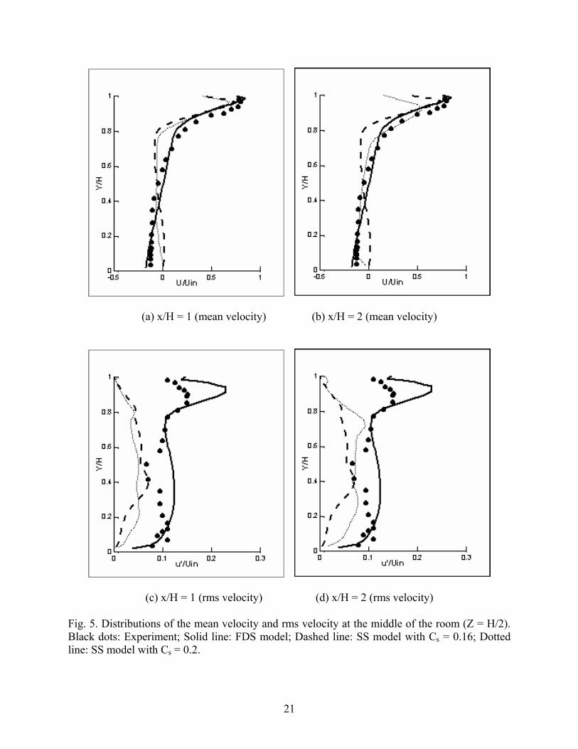
Fig. 5 shows the distributions of the mean velocity and rms velocity at two locations in the middle section of the room. It was found that the results computed with the FDS model agree reasonably with the experimental data. Although different Smagorinsky constants, Cs, are used for the SS model, the model still cannot correctly predict the flow field. During this study, the Cs value was increased from 0.16 to 0.2, but this increase does not necessarily lead to a higher kinetic energy (Fig. 5(c) and (d)). This is because the subgrid-scale eddy viscosity depends not only on Cs, but also on the strain rate and filter size (Eq. (7)). Therefore, increasing Cs does not

7

have an important impact on flows with a small strain rate. This suggests that for indoor airflow cases, in which walls normally have significant effects and both turbulent and laminar flows exist, the SS model may not be appropriate.

The distributions of the velocity field and the model coefficient, C, can show how the FDS model produces good results. Fig. 6 shows the mean flow field distributions at the middle section of the room. Fig. 6 (b) illustrates that C is small both near the walls and in the regions of laminar flow, which correctly represents the physics of flow motions.

4. Applications to natural ventilation

The previous section shows that both the SS and FDS models can correctly predict outdoor airflow. However, for indoor airflow, the performance of the SS model is not satisfactory due to its constant model coefficient. This section discusses natural ventilation in buildings with two subgrid-scale models. The natural ventilation combines both indoor and outdoor airflows. Two ventilation cases are considered: a single-sided ventilation and a cross ventilation case.

4.1 Single-sided ventilation

Dascalaki et al. [20] have done full-scale measurements for a single-opening house (Fig. 7). They measured the wind speeds at various heights in the middle section of the opening, and applied tracer gas decay method to measure the ventilation rate of the house. This study simulated one of their cases with two subgrid-scale models of LES and the standard k-ε model of RANS modeling. The RANS modeling was added to examine whether the RANS modeling technique is appropriate for single-sided ventilation studies. All of these numerical models use the same grid system, and the total grid number is 604,200. The Reynolds number is 5×105, and the non-dimensional characteristic length 3.3. So the expected Kolmogorov scale is about 10-4. The smallest non-dimensional grid size is 0.015, and the non-dimensional time step size is 0.002.

The simulation used the 1/7 power of the incoming wind profile. Table 1 gives the incoming wind information, in which WSn is the mean wind speed normal to the opening.

Table 1 Incoming wind information Mean wind speed at 1.5 m

(m/s) Mean WSn at 1.5 m

(m/s) Mean wind direction

(clockwise from south) 1.95 ± 0.52 0.98 ± 0.42 120 o

The experiment also measured the indoor air temperatures at different heights. Although the

temperature difference between indoor and outdoor airflows was 2.8 ± 0.1 oC, no significant air temperature stratification was observed during the measurement period. Dascalaki et al. [21] compared the importance of wind force and buoyancy force in single-sided natural ventilation with the Archimedes number, ArD,

( )102.0

UD/γ/γβΔTgH

ReGrAr 2

23

2D

D <<=== (13)

8

where Gr, ReD, β, g, H, D and U are Grashof number, Reynolds number, volumetric coefficient of expansion, gravitational force, the height of the opening, depth of the room and the wind speed at the building height, respectively. Eq. (13) shows that the natural convection due to a buoyancy effect is much smaller than the forced convection due to a wind effect. So for simplification, current simulation ignores the buoyancy effect.

Fig. 8 shows the distributions of the mean wind speed at the centerline of the opening. The standard k-ε model under-predicts the wind speeds at the bottom of the opening; the SS model over-predicts the speeds at the top; the FDS model agrees most reasonably with agreements with the experimental data in terms of the profile shape and magnitude. The FDS model performs better than the SS model in this case. This is because that the single-sided ventilation case involves fully developed turbulence flow around a building and laminar flow inside the building, where the turbulent and laminar flows have strong interactions at the opening (Fig. 9). Furthermore, the walls have an important effect on the flow motions. As seen in section 3.2, the SS model has difficulty in predicting the flows in which walls have significant effects and both turbulent and laminar patterns exist due to a constant model coefficient. Since the model coefficient in the FDS model varies corresponding to different flow types, the FDS might be more suitable to study the single-sided ventilation case, which involves many complex flows.

When studying natural ventilation in buildings, air change effectiveness is used to evaluate the ventilation performance. The air change effectiveness describes the ability of a ventilation system to deliver fresh air from the outside to the inside of a building [22]. These characteristics can be seen from the streamlines, as illustrated in Fig. 9. The streamlines in the instantaneous velocity field show that the fresh air can easily reach the wall opposite to the opening. However, the streamlines in the mean flow field illustrate a recirculation zone so that the air cannot enter deeply. The information from the mean flow field may restrict a designer to evaluate the ventilation performance for a particular design, and an instantaneous flow field can provide the needed information to the design.

The concept of the air change effectiveness shows that it cannot be determined by one index alone since the air change effectiveness ranges at each point of a room if the room air is not perfectly mixed, which is a common situation in natural ventilation. In order to use one standard for ventilation assessment, people introduced ventilation rate or air change rate, which describes the airflow rate introduced from outside into a building [22]. Although it is not an accurate measure of the ventilation performance of a building, ASHARE Standard 62 [23] uses ventilation rate to provide standard of proper minimum ventilation for acceptable indoor air quality.

Based on the definition, the ventilation rate in the numerical simulations can be computed by integrating the velocity at the opening. Appendix A derives the expressions for calculating the ventilation rate of a building (m3/s) with this integration method. There are two ways to do integral calculations. First one is to extract the mean velocity, Uj,k, from a mean flow field. The computed value can be called mean ventilation rate, Qmean.

∑ ∑= =

=jb

jaj

kb

kakkjkj,mean ΔzΔyU

21Q (14)

Since LES can provide instantaneous velocity field at each time step, another way to

compute the ventilation rate of a building is to accumulate and average the instantaneous

9

ventilation rates over a time period of T. The instantaneous ventilation rate at time tn is defined as

∑ ∑= =

=jb

jaj

kb

kakkj

nkj,

n ΔzΔyu21q (15)

So the accumulative instantaneous ventilation rate over a time period of T, Tins,Q , is defined as

∑

∑ ∑ ∑

=

= = =

⋅

= N

1n

n

N

1n

njb

jaj

kb

kakkj

nkj,

Tins,

Δt

Δt)ΔzΔyu(21

Q (16)

Eq. 16 shows that when computing the ventilation rate by accumulating and averaging instantaneous ventilation rate, the length of time over which the average is taken is important. In Qins,T, the subscript “T” shows the duration over which the Qins,T is computed.

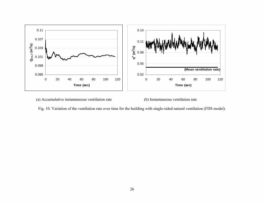
Fig. 10 shows the variations of the accumulative instantaneous ventilation rate, Qins,T, and the instantaneous ventilation rate, nq ,over time with the FDS model. Fig. 10 (a) shows that the distribution of Qins,T is broad for small values of T, and is narrow as T increases. When the averaging time T is increased to 120 seconds, Qins,T is narrowed to 0.101 m3/s, which is within an acceptable accuracy for the calculation of the accumulative instantaneous ventilation rate. So the time-interval over which Qins,T is calculated with the FDS model is 120 seconds. The variation of Qins,T over time with the SS model shows a similar distribution, and Qins,T is converted to 0.159 m3/s when T is increased to 120 seconds. For simplification, the result with the SS model is not shown in a figure. Fig. 10 (b) also includes the mean ventilation rate as a reference. It clearly shows that the averaging procedure used to calculate the mean ventilation rate significantly cancels out the instantaneous air exchange between the indoor and outdoor airflows, which has been theoretically proved in Appendix A. This can also be proved from the physical point of view. For example, an inflow in the upper part of the opening at one moment followed by an outflow at another moment can lead to a zero mean ventilation rate. However, the instantaneous ventilation rate is definitely not zero. Therefore, the mean ventilation rate is calculated to be much smaller than the accumulative instantaneous value, which should represent real conditions. Obviously, the instantaneous flow field is crucial for the correct determination of ventilation rates with single-sided natural ventilation.

Table 2 compares the air exchange rate obtained by different numerical methods with that from the experiment. The air exchange rate [22], which compares the ventilation rate of a room to the room volume, is also called air changes per hour (ACH). It is defined as

VQACH = (17)

10

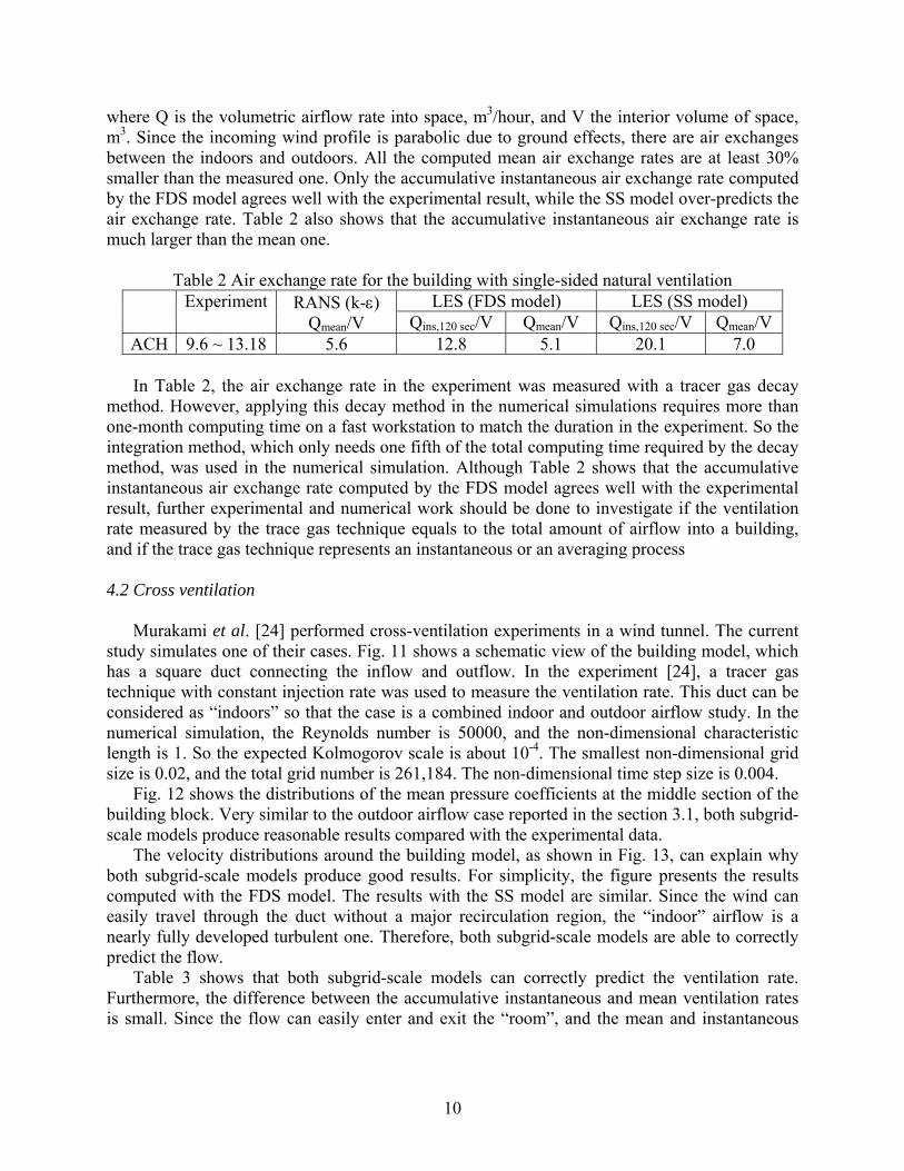
where Q is the volumetric airflow rate into space, m3/hour, and V the interior volume of space, m3. Since the incoming wind profile is parabolic due to ground effects, there are air exchanges between the indoors and outdoors. All the computed mean air exchange rates are at least 30% smaller than the measured one. Only the accumulative instantaneous air exchange rate computed by the FDS model agrees well with the experimental result, while the SS model over-predicts the air exchange rate. Table 2 also shows that the accumulative instantaneous air exchange rate is much larger than the mean one.

Table 2 Air exchange rate for the building with single-sided natural ventilation LES (FDS model) LES (SS model) Experiment RANS (k-ε)

Qmean/V Qins,120 sec/V Qmean/V Qins,120 sec/V Qmean/V ACH 9.6 ~ 13.18 5.6 12.8 5.1 20.1 7.0

In Table 2, the air exchange rate in the experiment was measured with a tracer gas decay

method. However, applying this decay method in the numerical simulations requires more than one-month computing time on a fast workstation to match the duration in the experiment. So the integration method, which only needs one fifth of the total computing time required by the decay method, was used in the numerical simulation. Although Table 2 shows that the accumulative instantaneous air exchange rate computed by the FDS model agrees well with the experimental result, further experimental and numerical work should be done to investigate if the ventilation rate measured by the trace gas technique equals to the total amount of airflow into a building, and if the trace gas technique represents an instantaneous or an averaging process 4.2 Cross ventilation

Murakami et al. [24] performed cross-ventilation experiments in a wind tunnel. The current study simulates one of their cases. Fig. 11 shows a schematic view of the building model, which has a square duct connecting the inflow and outflow. In the experiment [24], a tracer gas technique with constant injection rate was used to measure the ventilation rate. This duct can be considered as “indoors” so that the case is a combined indoor and outdoor airflow study. In the numerical simulation, the Reynolds number is 50000, and the non-dimensional characteristic length is 1. So the expected Kolmogorov scale is about 10-4. The smallest non-dimensional grid size is 0.02, and the total grid number is 261,184. The non-dimensional time step size is 0.004.

Fig. 12 shows the distributions of the mean pressure coefficients at the middle section of the building block. Very similar to the outdoor airflow case reported in the section 3.1, both subgrid-scale models produce reasonable results compared with the experimental data.

The velocity distributions around the building model, as shown in Fig. 13, can explain why both subgrid-scale models produce good results. For simplicity, the figure presents the results computed with the FDS model. The results with the SS model are similar. Since the wind can easily travel through the duct without a major recirculation region, the “indoor” airflow is a nearly fully developed turbulent one. Therefore, both subgrid-scale models are able to correctly predict the flow.

Table 3 shows that both subgrid-scale models can correctly predict the ventilation rate. Furthermore, the difference between the accumulative instantaneous and mean ventilation rates is small. Since the flow can easily enter and exit the “room”, and the mean and instantaneous

11

flow fields are similar, the corresponding ventilation rate calculated should be close to each other.

Table. 3 The ventilation rate in the cross ventilation case

SS model FDS model Qins,100 sec Qmean Qins,100 sec Qmean

Experiment Ventilation rate

(m3/s) 0.025 0.021 0.024 0.021 0.023

5. Conclusions

Two subgrid-scale models of LES, the SS model and the FDS model, have been used to simulate the outdoor and indoor airflow characteristics of natural ventilation. The study has led to the following conclusions.

(1) In the fully developed turbulence flow with a high Reynolds, most energy is contained in large eddies. The large eddies therefore play a more important role than the small eddies. Since both the SS and FDS models can directly solve the large-eddy motions, and can model the dissipative nature of turbulence, both models are able to provide accurate flow results for the most natural ventilation cases with fully or nearly fully developed turbulent flows. The flows investigated in this paper are the outdoor airflow and cross natural ventilation. Since the SS model is much simpler than the FDS model, and requires less computing time than that needed by the FDS model, the SS model is more suitable to solve for this type of problems.

(2) The SS model cannot predict laminar flows and the flows near walls because the model coefficient is a constant, and does not vary with flow type. The FDS model can give reasonable results in these cases because its model coefficient is a function of the flow type. The coefficient becomes zero in the near-wall and laminar regions, which correctly represents the physics of flow motions. Therefore, the FDS model is more appropriate to study natural ventilation flows with both turbulent and laminar characteristic, and for the near wall flow. The flows investigated in this paper are indoor airflow and single-sided natural ventilation with a simple geometry. To study the problems with a complex geometry or a large-scale site, however, LES has difficulty due to limitations of available memory and computing speed at present. So the RANS modeling would be a realistic choice in the near future [7]. Furthermore, for an internal ventilation study, the RANS modeling can produce reasonable result [8] with much less computing time than that required by LES, which makes the RANS modeling an obvious choice in this types of study.

(3) For single-sided ventilation, the information obtained from a mean flow field may restrict designers’ prospects about the ventilation performance of their design. This is because the averaging procedure of calculating the airflow significantly cancels out the instantaneous air exchange between indoor and outdoor air. So this procedure leads to lower ventilation rate and air change effectiveness than the instantaneous or measured ones. These findings conclude that the RANS modeling might not be appropriate for determining the ventilation rate and air change effectiveness due to the averaging procedure used in this model. The instantaneous flow field, which can be provided by LES, might be more useful to determine the ventilation rate and air change effectiveness in a single-sided natural ventilation design. However, this conclusion should be testified by further experimental and numerical work.

Appendix A. Calculation of airflow rate into a building with integration method

12

In CFD, the airflow rate into or out of a building can be calculated by integrating the normal velocity at all openings of a building if the flow is incompressible, which is true in most natural ventilation studies. Based on a mass balance of the airflow within a building, there will be as much fluid leaving the building in some regions, as there will be fluid entering the building. So the total amount of airflow out of a building equals to the total amount of airflow into a building, Qin = Qout. Therefore, in the integration calculation, if an absolute value sign is put around the velocity normal to the openings, we can get

∑ ∑= =

=+jb

jaj

kb

kakkjkj,outin ΔzΔyUQQ (A.1)

∑ ∑= =

=jb

jaj

kb

kakkjkj,in ΔzΔyU

21Q (A.2)

where [Δyja, Δyja+1, …, Δyjb] and [Δzka, Δzka+1, …, Δzkb] are the grid sizes in the y and z directions within the opening, respectively, and Uj,k is the mean normal velocity corresponding to the grid (Δyj, Δzk) at the openings. Note, the above calculation extracts Uj,k from a mean velocity field. So the computed airflow rate into a building can be called mean ventilation rate, Qmean. Since LES can provide instantaneous velocity field at each time step, the airflow rate into a building can be also calculated by accumulating and averaging the instantaneous ventilation rate over a time period of T. The instantaneous ventilation rate at time tn is defined as

∑ ∑= =

=jb

jaj

kb

kakkj

nkj,

n ΔzΔyu21q (A.3)

So the accumulative instantaneous ventilation rate over a time period of T, Tins,Q , is defined as

∑

∑ ∑ ∑

=

= = =

⋅

= N

1n

n

N

1n

njb

jaj

kb

kakkj

nkj,

Tins,

Δt

Δt)ΔzΔyu(21

Q

T

ΔzΔyΔtu21 jb

jaj

kb

kakkj

N

1n

nnkj,∑ ∑ ∑

= = == (A.4)

where n

kj,u is the instantaneous normal velocity at the opening at time tn, Δtn is the time step size; (tn+1–tn), and N is the total number of the time steps, during which Qins,T is calculated. Since the relationship between the mean velocity, Uj,k, and the instantaneous velocity uj,k, is

13

T

ΔtuU

N

1n

nnkj,

kj,

∑=

⋅= (A.5)

Eq. (A.2) can be derived as

T

ΔzΔyΔtu21

Q

jb

jaj

kb

kakkj

N

1n

nnkj,

mean

∑ ∑ ∑= = == (A.6)

Since

∑∑==

≥N

1n

nnkj,

N

1n

nnkj, ΔtuΔtu (Δt n > 0) (A.7)

We can get

≥∑ ∑ ∑= = =

T

ΔzΔyΔtu21 jb

jaj

kb

kakkj

N

1n

nnkj,

T

ΔzΔyΔtu21 jb

jaj

kb

kakkj

N

1n

nnkj,∑ ∑ ∑

= = =

meanTins, QQ ≥ (A.8)

In Eq. (A.7), only when n

kj,u keeps the same sign over the whole time period of T, which means

that nkj,u should be always negative or positive, Qins,T can equal to Qmean. This situation may

happen in a simple cross-ventilation case, such as a tunnel type. However, for complex ventilation type, such as single-sided ventilation, the instantaneous velocity at an opening changes direction all the time due to strong interactions between turbulent and laminar flows. Acknowledgment

This work is supported by the U.S. National Science Foundation under grant CMS-9877118. References: [1] J.J. Finnegan, C.A.C. Pickering, and P.S. Burge, The sick building syndrome: prevalence studies, British Medical J. 289 (1984) 1573-1575. [2] J.F. Busch, A tale of two populations: thermal comfort in air-conditioned and naturally ventilated offices in Thailand, Energy and Buildings 18 (3-4) (1992) 235-249.

14

[3] L. Davidson and P. Nielsen, Large eddy simulation of the flow in a three-dimensional ventilation room, 5th International Conference on Air Distribution in Rooms, ROOMVENT’96, July 17-19, 1996. [4] W. Zhang and Q. Chen, Large eddy simulation of indoor airflow with a filtered dynamic subgrid scale model, International J. of Heat and Mass Transfer 43 (17) (2000) 3219-3231. [5] W. Rodi, J.H. Ferziger, M. Breuer and M. Pourquié, Status of large eddy simulation: results of a workshop, J. of Fluids Eng. 119 (1997) 248-262. [6] S. Murakami, Overview of turbulence models applied in CWE-1997, J. of Wind Eng. Ind. Aerodyn. 74-76 (1998) 1-24. [7] H. Hangan, F. McKenty, L. Gravel and R. Camarero, Internal ventilation study for complex architectural geometry, Proceedings of the 10th International Conference on Wind Engineering, Copenhagen, Denmark, June 21-24, 1999, Vol. 3, 1933-1938. [8] X. Yuan, Q. Chen, L.R. Glicksman, Y. Hu, and X. Yang, Measurements and computations of room airflow with displacement ventilation, ASHRAE Transactions 105(1) (1999) 340-352. [9] D. Lakehal and W. Rodi, Calculation of the flow past a surface-mounted cube with two-layer turbulence models, J. of Wind Eng. Ind. Aerodyn. 67/68 (1997) 65-78. [10] J. Smagorinsky, General circulation experiments with the primitive equations. I. The basic experiment, Monthly Weather Review 91 (1963) 99-164. [11] J.W. Deardorff, A numerical study of three-dimensional turbulent channel flow at large Reynolds numbers, J. Fluid Mech. 41 (1970) 453-480. [12] M. Germano, U. Piomelli, P. Moin, and W.H. Cabot, A dynamic subgrid-scale eddy viscosity model, Phys. Fluids A 3 (7) (1991) 1760-1765. [13] D.K. Lilly, A proposed modification of Germano subgrid-scale closure method, Phys. Fluids A 4 (3) (1992) 633-635. [14] F.H. Harlow and J.E. Welch, Numerical calculation of time-dependent viscous incompressible flow, Phys. Fluids 8 (12) (1965) 2182-2189. [15] H.L. Stone, Iterative solution of implicit approximations of multidimensional partial differential equations, SIAM J. Numerical Analysis 5 (3) (1968) 530-558. [16] K.B. Shah, Large eddy simulations of flow past a cubic obstacle, Ph.D. dissertation, Department of Mechanical Engineering, Stanford University, 1998. [17] R. Mittal and P. Moin, Suitability of upwind-biased finite-difference schemes for large eddy simulation of turbulent flows, AIAA J. 35 (8) (1997) 1415-1417. [18] AIJ Working Group, Numerical Prediction of Wind Loading on Buildings and Structures, Division for Wind Loading Design, Architecture Institute of Japan (in Japanese) (1994). [19] P.V. Nielsen, A. Restivo and J.H. Whitelaw, The velocity characteristics of ventilated room, J. Fluids Eng. 100 (1978) 291-298. [20] E. Dascalaki, M. Santamouris, A. Argiriou, C. Helmis, D. Asimakopoulos, K. Papadopoulos and A. Soilemes, On the combination of air velocity and flow measurements in single sided natural ventilation configurations, Energy and Buildings 24 (1996) 155-165. [21] E. Dascalaki, M. Santamouris, A. Argiriou, C. Helmis, D. Asimakopoulos, K. Papadopoulos and A. Soilemes, Predicting single sided natural ventilation rates in buildings, Solar Energy 55 (5) (1995) 327-341. [22] ASHRAE Fundamentals Handbook, Ventilation and infiltration (Chapter 25), American Society of Heating, Refrigerating and Air-Conditioning Engineers, Inc., Atlanta, GA (1997). [23] ASHRAE Standard 62-1999, Ventilation for acceptable indoor air quality, American Society of Heating, Refrigerating and Air-Conditioning Engineers, Inc., Atlanta, GA (1999).

15

[24] S. Murakami, S. Kato, S. Akabayashi, K. Mizutani and Y.D. Kim, Wind tunnel test on velocity-pressure field of cross-ventilation with open windows, ASHRAE Transactions 97 part 1 (1991) 525-538.

16

Figure captions Fig. 1. The computational domain for the flow over a bluff body (top figure is the section view and bottom figure is the plan view). Fig. 2. Distributions of the mean pressure coefficients. Black dots with error bars: Experiment; Solid line: SS model; Dashed line: FDS model. (a) middle section of the block (b) plan at height of H/2 Fig. 3. Contributions of different terms to the mean flow in the momentum equation at the middle section of the block.

(a) in front of the block (b) along the roof (c) behind the block Fig. 4. Sketch of forced convection in a room. Fig. 5. Distributions of the mean velocity and rms velocity at the middle of the room (Z = H/2). Black dots: Experiment; Solid line: FDS model; Dashed line: SS model with Cs = 0.16; Dotted line: SS model with Cs = 0.2.

(a) x/H = 1 (mean velocity) (b) x/H = 2 (mean velocity) (c) x/H = 1 (rms velocity) (d) x/H = 2 (rms velocity)

Fig. 6. Distributions of the mean flow field and the mean model coefficient, C, at the middle section of the room

(a) velocity field (b) model coefficient, C Fig. 7. A sketch of the single-opening house. Fig. 8. The profiles of the mean wind speed at the centerline of the opening. Black dots with error bars: Experiment; Solid line: FDS model; Dashed line: SS model; Dash-dot line: standard k-ε model. Fig. 9. Flow field with the streamlines at the middle section of the room computed by LES with the FDS model.

(a) mean (b) instantaneous Fig. 10. Variation of the ventilation rate over time for the building with single-sided natural ventilation (FDS model).

(a) Accumulative instantaneous ventilation rate (b) Instantaneous ventilation rate Fig. 11. A schematic view of the building model. Fig. 12. The mean pressure distribution at the middle section of the building block. Black dots: Experiment; Solid line: SS model; Dashed line: FDS model. Fig. 13. The velocity distributions for the cross ventilation with the FDS model.

(a) mean (b) instantaneous

17

-H

10H

-10H-10H

20H

6H

H

0

Z

H

Y

OutflowInflow

X

X

-H H

Fig. 1. The computational domain for the flow over a bluff body (top figure is the section view and bottom figure is the plan view).

18

-1.5

-1

-0.5

0

Cp

Cp00.511.5

Cp-1.5-1-0.50

(a) middle section of the block

Cp00.511.5

Cp-1.5-1-0.50

-1.5

-1

-0.5

0

-1.5

-1

-0.5

0

(b) plan at height of H/2 Fig. 2. Distributions of the mean pressure coefficients. Black dots with error bars: Experiment; Solid line: SS model; Dashed line: FDS model.

19

(a) in front of the block (b) along the roof (c) behind the block

Fig. 3. Contributions of different terms to the mean flow in the momentum equation at the middle section of the block.

20

Fig. 4. Sketch of

forced convection in a room.

Hhout = 0.48mL/H = 3

hin = 0.168m Uin = 0.455m/s

W/H = 1

X

Y

Z

21

(a) x/H = 1 (mean velocity) (b) x/H = 2 (mean velocity)

(c) x/H = 1 (rms velocity) (d) x/H = 2 (rms velocity) Fig. 5. Distributions of the mean velocity and rms velocity at the middle of the room (Z = H/2). Black dots: Experiment; Solid line: FDS model; Dashed line: SS model with Cs = 0.16; Dotted line: SS model with Cs = 0.2.

22

X

Y

(a) velocity field

(b) model coefficient, C

Fig. 6. Distributions of the mean flow field and the mean model coefficient, C, at the middle section of the room

23

3.3m

2.4m 2m

1.3m 1m 1.3m

N

Fig. 7. A sketch of the single-opening house.

24

Wind Speed (m/s)

H(

m)

0 0.5 1 1.50

0.5

1

1.5

2

Exp.SS modelFDS modelk-e model

Fig. 8. The profiles of the mean wind speed at the centerline of the opening. Black dots with error bars: Experiment; Solid line: FDS model; Dashed line: SS model; Dash-dot line: standard k-ε model.

25

(a) mean (b) instantaneous

Fig. 9. Flow field with the streamlines at the middle section of the room computed by LES with the FDS model.

26

0.095

0.098

0.101

0.104

0.107

0.11

0 20 40 60 80 100 120

Time (sec)

Qin

s,T

(m3 /s

)

(Mean ventilation rate)0.02

0.05

0.08

0.11

0.14

0 20 40 60 80 100 120

Time (sec)

qn (m3 /s

)

(a) Accumulative instantaneous ventilation rate (b) Instantaneous ventilation rate

Fig. 10. Variation of the ventilation rate over time for the building with single-sided natural ventilation (FDS model).

27

H

H

H

H/6 H/6

Wind

z

y

x

Fig. 11. A schematic view of the building model.

28

C p -1-0.50

C p 00.51

- 0 . 5

0

0 . 5

1 C p

Windward wall Leeward wall

Along floor Fig. 12. The mean pressure distribution at the middle section of the building block. Black dots: Experiment; Solid line: SS model; Dashed line: FDS model.

29

Section

Plan

Section

Plan

(a) Mean (b) Instantaneous

Fig. 13. The velocity distributions for the cross ventilation with the FDS model.