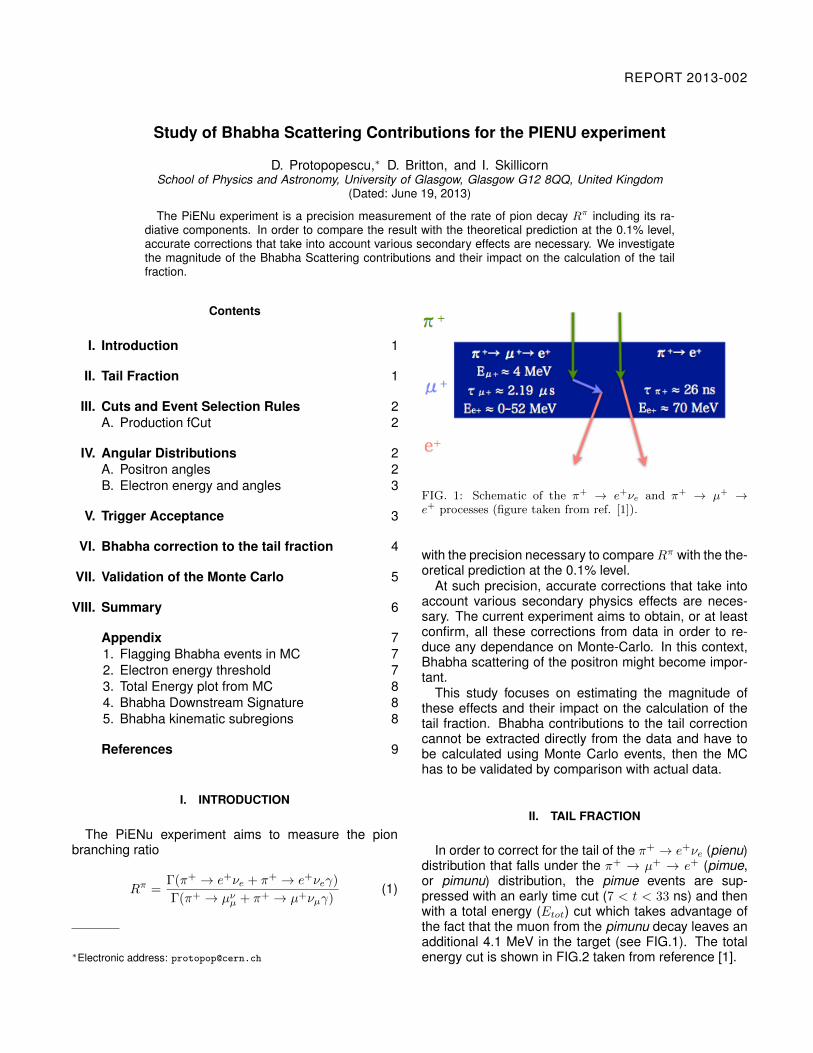
REPORT 2013-002

Study of Bhabha Scattering Contributions for the PIENU experiment

D. Protopopescu,⇤ D. Britton, and I. SkillicornSchool of Physics and Astronomy, University of Glasgow, Glasgow G12 8QQ, United Kingdom

(Dated: June 19, 2013)

The PiENu experiment is a precision measurement of the rate of pion decay R⇡ including its ra-diative components. In order to compare the result with the theoretical prediction at the 0.1% level,accurate corrections that take into account various secondary effects are necessary. We investigatethe magnitude of the Bhabha Scattering contributions and their impact on the calculation of the tailfraction.

Contents

I. Introduction 1

II. Tail Fraction 1

III. Cuts and Event Selection Rules 2A. Production fCut 2

IV. Angular Distributions 2A. Positron angles 2B. Electron energy and angles 3

V. Trigger Acceptance 3

VI. Bhabha correction to the tail fraction 4

VII. Validation of the Monte Carlo 5

VIII. Summary 6

Appendix 71. Flagging Bhabha events in MC 72. Electron energy threshold 73. Total Energy plot from MC 84. Bhabha Downstream Signature 85. Bhabha kinematic subregions 8

References 9

I. INTRODUCTION

The PiENu experiment aims to measure the pionbranching ratio

R⇡ =�(⇡+ ! e+⌫

e

+ ⇡+ ! e+⌫e

�)

�(⇡+ ! µ⌫

µ

+ ⇡+ ! µ+⌫µ

�)(1)

⇤Electronic address: protopop@cern.ch

FIG. 1: Schematic of the ⇡+ ! e+⌫e

and ⇡+ ! µ+ !e+ processes (figure taken from ref. [1]).

with the precision necessary to compare R⇡ with the the-oretical prediction at the 0.1% level.

At such precision, accurate corrections that take intoaccount various secondary physics effects are neces-sary. The current experiment aims to obtain, or at leastconfirm, all these corrections from data in order to re-duce any dependance on Monte-Carlo. In this context,Bhabha scattering of the positron might become impor-tant.

This study focuses on estimating the magnitude ofthese effects and their impact on the calculation of thetail fraction. Bhabha contributions to the tail correctioncannot be extracted directly from the data and have tobe calculated using Monte Carlo events, then the MChas to be validated by comparison with actual data.

II. TAIL FRACTION

In order to correct for the tail of the ⇡+ ! e+⌫e

(pienu)distribution that falls under the ⇡+ ! µ+ ! e+ (pimue,or pimunu) distribution, the pimue events are sup-pressed with an early time cut (7 < t < 33 ns) and thenwith a total energy (E

tot

) cut which takes advantage ofthe fact that the muon from the pimunu decay leaves anadditional 4.1 MeV in the target (see FIG.1). The totalenergy cut is shown in FIG.2 taken from reference [1].

2

FIG. 2: Etot

spectrum, as shown in Fig. 5.1 from reference [1].The vertical red lines correspond to the cut 15.7 < E

tot

< 16.8MeV. See FIG.11 from Appendix 3 for comparison.

The quantity Etot

, on which the above cut is based, isthe sum of the energies deposited in the target (Tg) andupstream counters (B1, B2, S1, S2):

Etot

= EB1 + E

B2 + ES1 + E

S2 + ETg

(2)

Positrons that Bhabha scatter in the target will pro-duce an electron that deposits additional energy in thetarget, thus raising the energy in the E

tot

spectrum, withthe effect that such events are excluded from the se-lected region.

In this study, we consider only positrons that undergoBhabha scattering within the target volume. Bhabhascattering downstream of the target is irrelevant in thatit can not affect E

tot

defined by Eq.(2). Bhabha scatter-ing upstream of the target would occur for decay-in-flight(PDIF) events but this is (a) known to be a very smallcontribution and (b) at least partially addressed by othercuts (e.g. kink cut [1]).

III. CUTS AND EVENT SELECTION RULES

The following cuts and selection rules are used in [1]and in this analysis:

C1. One ⇡+ in B1 and B2: (NB1 = 1 & N

B2 = 1 &PID

B1 = 211 & PIDB2 = 211)

C2. The ⇡+ decays at rest, in target: (a) p⇡+decay

= 0

& (b) |z⇡+decay

| < 4 mm

C3. Trigger thresholds: ET2 > 0.1 MeV & E

T1 > 0.1MeV

C4. WC3 radial cut: RWC3 < 60 mm

where NBx

is the number of hits in detector Bx, andPID

Bx

is the particle id of the hit in detector Bx.Events containing a Bhabha scattered electron can be

selected at MC truth level with the conditions:

C5. Bhabha scattering flag: EBh

> 0 & Eele

> 0

The quantity EBh

is used in SteppingAction to flagevents including G4eIonisation processes (i.e. ioniza-tion and energy loss by electrons and positrons) occur-ring in the ”Target” volume (see Appendix 1). In suchcase, E

Bh

will contain the energy of the positron. Con-dition E

ele

> 0 ensures that the outgoing electron hasnot stopped immediately after undergoing Bhabha scat-tering [6].

A. Production fCut

During our investigation of the electron energy dis-tribution we have noticed that an artificial thresholdof 2 MeV was present. Looking at the definitionsof the materials in the MC, we have discovered thatthis threshold was affecting all the materials coded inthe Materials.cc file, but none from the G4 materialsdatabase. The problem was traced to a forgotten pro-duction cut

Cuts->SetProductionCut(10*mm); (3)

in file WorldConstructor.cc [4]. This fCut was overrid-ing all values set in the PhysicsList.cc,

defaultCutValue = 1.0*mm;

fCutForGamma = 1.0*mm;

fCutForElectron = 0.1*mm; (4)fCutForPositron = 0.1*mm;

and had to be removed in order to obtain a correct MCsimulation of the PiENu physics. See Appendix 2 formore details.

One should note that the Monte Carlo results shown inreference [1] were based on the incorrect cut (3), whileall results presented in this report employ the correct set-tings (4). Results obtained with the two settings (3 and4) are compared in Appendix 4.

IV. ANGULAR DISTRIBUTIONS

To be able to select a predominantly Bhabha subsam-ple for a comparison between MC and data, it is impor-tant to understand the geometry of Bhabha events.

A. Positron angles

When selecting MC events where the e+ Bhabhascatters in the target, we obtain an angular distributionpeaked around 90�. This is explained by the fact that theprobability of Bhabha scattering depends on the amountof target material traversed by the positron and this, dueto the geometry of the target, is dependent on the angle

3

(✓e+) of the positron with respect to the beam direction.

FIG.3 shows the ✓e+ distribution obtained from Monte

Carlo.

B. Electron energy and angles

Electrons resulting from Bhabha scattering in the tar-get are selected as shown in Appendix 1. Their angulardistribution and energy spectrum are shown in FIG.4.

The scattered electrons carry little momentum and thedirection of the positron is not significantly altered bythe Bhabha scattering. FIG.5 illustrates this by showingthe correlation between the angles of the original andBhabha-scattered positrons.

V. TRIGGER ACCEPTANCE

Since the majority of Bhabha scattered positrons aretravelling perpendicular to the beam direction, they aremuch less likely to give a trigger than normal events. Ap-plying the trigger conditions C3+C4 in the Monte Carlo,we find the distribution shown in FIG.6. This require-ment reduces the number of Bhabha events by a factorof ⇡1/9.

FIG.6 (top) can be understood, qualitatively, as fol-lows: the large peak at smaller angles corresponds tothe case where the trigger was made by the positron.The residue above 60� is due to triggers made byBhabha scattered electrons.

e+θ0 20 40 60 80 100 120 140 160 180

0

500

1000

1500

2000

2500

Entries 158614

FIG. 3: Angular distribution of Bhabha scattered positronsfrom MC. Conditions C1+C2+C5 are applied here and ✓angles are measured w.r.t. the beam direction (⇡+ !e+⌫

e

Monte Carlo).

e−θ0 20 40 60 80 100 120 140 160 180

0

200

400

600

800

1000

1200

Entries 158614

[MeV]e−E0 2 4 6 8 10 12 14 16 18 20

1

10

210

310

410

510

Entries 158614

FIG. 4: Theta angle ✓e� and kinetic energy E

e� of theBhabha-scattered electron when conditions C1+C2+C5 areapplied (⇡+ ! e+⌫

e

Monte Carlo).

This interpretation can be supported by looking atthe energy of the Bhabha particles in the NaI detector,shown in FIG.7. We have seen in FIG.4 that the Bhabhaelectron has predominantly low energies and thus wewould expect that events with ✓

e+ > 60� should corre-spond to low energy events in the NaI (which detectsthe triggering electron) and events in the lower peak(✓

e+ < 60�) should correspond to higher energy eventsin the NaI detector (which, in this case, has detected thetriggering positron that still has most of the 70 MeV).

From the ⇡+ ! e+⌫e

distributions in FIG.7 (top)one can extract a rough estimate of the percentage of

4

[deg]1e+

θ0 20 40 60 80 100 120 140

[d

eg

]e

+θ

0

20

40

60

80

100

120

140

Entries 158614

e+e-θ

20 40 60 80 100 120 140 160 180

3 1

0×

0

5

10

15

20

25

FIG. 5: Top: ✓e+ angle of the scattered positron plotted

versus the ✓0e+ angle of the positron originating from the

⇡+ decay in the target. Conditions C1+C2+C5 are appliedhere and ✓ angles are measured w.r.t. beam direction. Bot-tom: Angle between the Bhabha scattered e+and e� (from⇡+ ! e+⌫

e

MC truth level). Same cuts.

Bhabha events where the trigger is given by the Bhabhaelectron, which was found to be ⇡ 1.5%.

VI. BHABHA CORRECTION TO THE TAIL FRACTION

The Bhabha correction to the tail fraction is calculatedusing Monte Carlo events, and then the values obtained

e+θ0 20 40 60 80 100 120 140 160 180

0

100

200

300

400

500

600

Entries 18313

e−θ0 20 40 60 80 100 120 140 160 180

0

50

100

150

200

250

Entries 18313

FIG. 6: Theta distribution of Bhabha-scattered positrons(top) and electrons (bottom) from ⇡+ ! e+⌫

e

Monte Carlo,after acceptance and trigger conditions C1+C2+C3+C4+C5are applied. Compare with FIG.3 and FIG.4.

must be validated by comparison of the Bhabha effectsin the MC and data.

FIG.8 shows the (ENaI

+ ECsI

) spectrum when vari-ous cuts (explained in the caption) are applied. We de-fine here the tail fraction as the ratio between the num-bers of counts below and above 50 MeV. The Bhabha

correction to the tail fraction is obtained by calculatingthe same ratio for Bhabha events, i.e. with condition C5added.

A calculation done using an extended Monte Carlo

5

[MeV]NaIE0 10 20 30 40 50 60 70 80

1

10

210

310

Pienu Bhabhas

electron trigger

positron trigger

[MeV]NaIE0 10 20 30 40 50 60 70 80

10

210

310Pimue Bhabhas

electron trigger

positron trigger

FIG. 7: Energy deposited in the NaI detector (BINA)by Bhabha-scattered particles, from ⇡+ ! e+⌫

e

MonteCarlo. Here conditions C1+C2+C3+C4+C5 are combinedwith ✓

e+ < 60� (brown), and ✓e+ > 60� (blue). See ✓

e+ dis-tribution from FIG.6 (top). Bottom plot shows the same for⇡+ ! µ+ ! e+ for comparison.

event sample [4] gives the values:

fT

= 0.01904± 0.00008

f c

T

= 0.00896± 0.00006 (5)bT

= 0.0101± 0.0001

where by fT

we denoted the tail fraction and f c

T

is the tailfraction with E

tot

cut, and bT

is the Bhabha correction tothe tail fraction.

[MeV]CsI+ENaIE0 10 20 30 40 50 60 70

1

10

210

310

410eν + e→ +π Spectrum from CsI+ENaIE

(1) Acceptance cuts only

cut addedtot

(2) E

(3) Bhabha events in (2)

FIG. 8: Sum of the energies deposited in the NaI and CsIdetectors, from ⇡+ ! e+⌫

e

MC. Conditions C1+C2+C3+C4are applied (green). For the suppressed spectrum (light blue),the condition 15.7 < E

tot

< 16.8 MeV is applied. The Bhabhacontribution (dark blue) is obtained by adding condition C5.

For comparison, the same calculation done using theincorrect Monte Carlo production cut (3) was giving thevalues

fT

= 0.01585± 0.00007

f c

T

= 0.00887± 0.00006 (6)bT

= 0.0069± 0.0001

which are significantly different.This Bhabha correction is calculated using Monte

Carlo events, so the next step is to validate our MC bymaking a comparison of the Bhabha effects in our simu-lations and the actual data.

These results should be updated and should includehere details on how the the systematic uncertainty onthe Bhabha correction to the tail fraction was obtained.

VII. VALIDATION OF THE MONTE CARLO

We’ve seen that the Bhabha correction to the tail frac-tion cannot be extracted directly from the data and hadto be calculated using Monte Carlo events. In order toverify the obtained value, one would have to (A) find away to select a kinematic region where the Bhabha con-tribution is high enough, (B) find out if this can be mea-sured precisely enough in the data, (C) compare the MCprediction with the measurement.

Several routes were tried, by looking at:

R1. 2-dimensional plots of the deposited energies inthe detectors upstream of the target versus E

tot

6

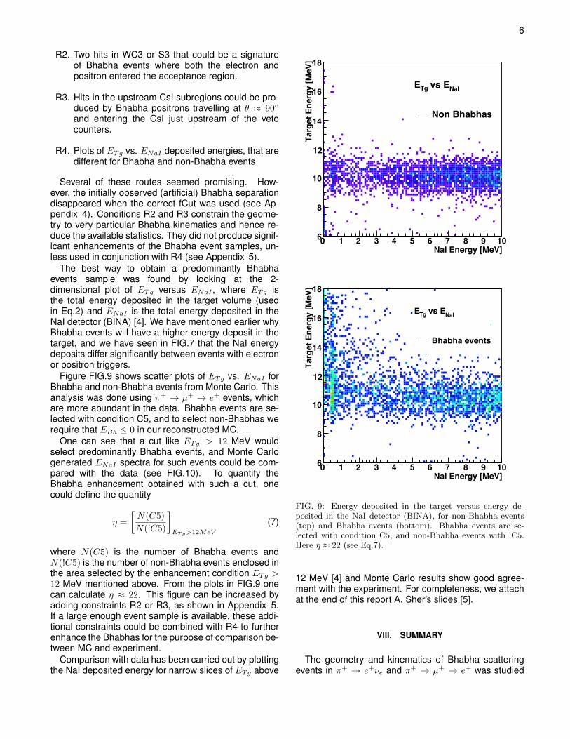
R2. Two hits in WC3 or S3 that could be a signatureof Bhabha events where both the electron andpositron entered the acceptance region.

R3. Hits in the upstream CsI subregions could be pro-duced by Bhabha positrons travelling at ✓ ⇡ 90�

and entering the CsI just upstream of the vetocounters.

R4. Plots of ETg

vs. ENaI

deposited energies, that aredifferent for Bhabha and non-Bhabha events

Several of these routes seemed promising. How-ever, the initially observed (artificial) Bhabha separationdisappeared when the correct fCut was used (see Ap-pendix 4). Conditions R2 and R3 constrain the geome-try to very particular Bhabha kinematics and hence re-duce the available statistics. They did not produce signif-icant enhancements of the Bhabha event samples, un-less used in conjunction with R4 (see Appendix 5).

The best way to obtain a predominantly Bhabhaevents sample was found by looking at the 2-dimensional plot of E

Tg

versus ENaI

, where ETg

isthe total energy deposited in the target volume (usedin Eq.2) and E

NaI

is the total energy deposited in theNaI detector (BINA) [4]. We have mentioned earlier whyBhabha events will have a higher energy deposit in thetarget, and we have seen in FIG.7 that the NaI energydeposits differ significantly between events with electronor positron triggers.

Figure FIG.9 shows scatter plots of ETg

vs. ENaI

forBhabha and non-Bhabha events from Monte Carlo. Thisanalysis was done using ⇡+ ! µ+ ! e+ events, whichare more abundant in the data. Bhabha events are se-lected with condition C5, and to select non-Bhabhas werequire that E

Bh

0 in our reconstructed MC.One can see that a cut like E

Tg

> 12 MeV wouldselect predominantly Bhabha events, and Monte Carlogenerated E

NaI

spectra for such events could be com-pared with the data (see FIG.10). To quantify theBhabha enhancement obtained with such a cut, onecould define the quantity

⌘ =

N(C5)

N(!C5)

�

ETg>12MeV

(7)

where N(C5) is the number of Bhabha events andN(!C5) is the number of non-Bhabha events enclosed inthe area selected by the enhancement condition E

Tg

>12 MeV mentioned above. From the plots in FIG.9 onecan calculate ⌘ ⇡ 22. This figure can be increased byadding constraints R2 or R3, as shown in Appendix 5.If a large enough event sample is available, these addi-tional constraints could be combined with R4 to furtherenhance the Bhabhas for the purpose of comparison be-tween MC and experiment.

Comparison with data has been carried out by plottingthe NaI deposited energy for narrow slices of E

Tg

above

Target Energy [MeV]11 11.5 12 12.5 13 13.5 140

100

200

300

400

500

Target Energy

Non Bhabhas

Bhabha events

NaI Energy [MeV]0 1 2 3 4 5 6 7 8 9 10

Targ

et E

nerg

y [M

eV]

6

8

10

12

14

16

18

NaI vs ETgE

Non Bhabhas

NaI Energy [MeV]0 1 2 3 4 5 6 7 8 9 10

Cou

nts

20

40

60

80

100

120

140

160

NaI Energy [MeV]0 1 2 3 4 5 6 7 8 9 10

Targ

et E

nerg

y [M

eV]

6

8

10

12

14

16

18

NaI vs ETgE

Bhabha events

FIG. 9: Energy deposited in the target versus energy de-posited in the NaI detector (BINA), for non-Bhabha events(top) and Bhabha events (bottom). Bhabha events are se-lected with condition C5, and non-Bhabha events with !C5.Here ⌘ ⇡ 22 (see Eq.7).

12 MeV [4] and Monte Carlo results show good agree-ment with the experiment. For completeness, we attachat the end of this report A. Sher’s slides [5].

VIII. SUMMARY

The geometry and kinematics of Bhabha scatteringevents in ⇡+ ! e+⌫

e

and ⇡+ ! µ+ ! e+ was studied

7

Target Energy [MeV]11 11.5 12 12.5 13 13.5 14

Co

un

ts

0

100

200

300

400

500

Entries 69505

Target Energy

Non Bhabhas

Bhabha events

FIG. 10: Comparison of energies deposited in the target fornon-Bhabha and Bhabha events. Bhabha events are selectedwith condition C5, and non-Bhabha events with !C5. Same⌘ ⇡ 22 (see Eq.7).

using simulated events. Once Bhabha scattering wasunderstood, its contribution to the tail fraction was esti-mated from Monte Carlo. What remained was to verifythe predictions or our MC by comparing them with thedata, within the kinematic regions of interest.

After investigating the angular distribution of theBhabha scattered e� and e+, we have found that basedon the geometry and energy characteristics of Bhabhascattering events it is possible to use reconstruction-level cuts to separate a predominantly Bhabha subsam-ple in the data. This sample was then compared withour Monte Carlo and a good match was found.

Hence, our study supports applying the Bhabha cor-rection to the tail fraction estimated from Monte Carlo tothe actual data.

Appendix

1. Flagging Bhabha events in MC

Bhabha scattering events are flagged inSteppingAction, by assigning to E

Bh

the energyof the positron if the process involved at a certain step

is ”eIoni” and the volume where this occurs is ”Target”

if (theParticleName == "e+"

&& thePostVolume == "/pienu/Target"

&& theProcessName == "eIoni") {

runAction->TgtBhabha(postEnergy);

}

The energies and momenta of the initial positron andthe outgoing positron and electron are recorded with thefollowing conditionals:

if(theParticleName == "e+"

&& thePostVolume == "/pienu/Target"

&& theProcessName == "eIoni"){

runAction->PositronFromBhabha(postEnergy,

postMomentum);

runAction->PositronPreBhabha(preEnergy,

preMomentum);

}

if(theParticleName == "e-"

&& thePostVolume == "/pienu/Target"

&& theCreatorProcessName == "eIoni"

&& theTrack->GetCurrentStepNumber()==1){

runAction->ElectronFromBhabha(prePosition,

preEnergy, preMomentum);

}

The ”eIoni” physics processes are implemented inmodule G4MollerBhabhaModel.cc from the Geant4 MCsimulation package [2].

2. Electron energy threshold

The energy threshold for e� produced in the scintil-lator material was set at 2.19 MeV by a 1 cm Produc-tionCut in WorldContructor.cc. Here is the output fromDumpCutValuesTable():

Index : 13 used in the geometry : Yes

recalculation needed : No

Material : Scintillator

Range cuts : gamma 1 cm

e- 1 cm

e+ 1 cm

proton 1 cm

Energy thresholds : gamma 5.71952 keV

e- 2.18887 MeV

e+ 2.0743 MeV

proton 1 MeV

In this case all Bhabha electrons under 2.19 MeV wereabsorbed in the Scintillator (i.e. never produced). Whenthis (incorrect) setting was removed and the actualphysics cuts from PhysicsList.cc are used, the energythreshold drops to 86.4 keV:

Index : 11 used in the geometry : Yes

recalculation needed : No

Material : Scintillator

Range cuts : gamma 1 mm

e- 100 um

e+ 100 um

proton 1 mm

Energy thresholds : gamma 2.40367 keV

8

Total Energy [MeV]14 16 18 20 22 24

Co

un

ts

1

10

210

310

from MCtot

E

pimunu (1)pienu (2)sum of (1) and (2)

FIG. 11: Total energy plot from MC. Conditions applied:C1+C2b+C3+C4. Compare this with FIG.2.

e- 86.3829 keV

e+ 85.2297 keV

proton 100 keV

Approximately 15 times more Bhabha scattered elec-trons are produced with this threshold, some of whichcan exit the target and produce a trigger.

3. Total Energy plot from MC

We have tried to replicate Figure 5.1 from [1] with theMonte Carlo. With no pileup and no radiative effectsadded, the result is shown in FIG.11. One should com-pare this with FIG.2.

4. Bhabha Downstream Signature

Using the 1cm MC production cut, we have noticedthat Bhabha scattered electrons and positrons fromevents that produce a trigger had a slightly different sig-nature in S3, T1 and T2 than ’normal’ events. This isbecause the the extra electron will deposit an additionalenergy downstream of the target as well.

We have tried various combinations of S3, T1 and T2energy deposits and we have found that the E

S3 + ET1

gave the best separation, shown in FIG.12 (top).This seemed a promising avenue until we have dis-

covered the incorrect electron energy threshold in theMC. And once the correct fCut (4) is used in the MonteCarlo, the separation completely disappears, as seen inFIG.12 (bottom).

5. Bhabha kinematic subregions

Efforts were made to obtain a Bhabha events sampleas pure as possible. In theory, this could be achievedby further constraining the kinematics to preferentially

[MeV]totE14 15 16 17 18 19 20 21 22 23

E(S

3+

T1)

[MeV

]

0

0.5

1

1.5

2

2.5

3

3.5

4

4.5

5

totE(S3+T1) vs. E

MC pimunu (1)

MC pienu (2)

Bhabha events in (2)

[MeV]totE14 15 16 17 18 19 20 21 22 23

E(S

3+

T1)

[MeV

]

0

0.5

1

1.5

2

2.5

3

3.5

4

4.5

5

totE(S3+T1) vs. E

MC pimunu (1)

MC pienu (2)

Bhabha events in (2)

FIG. 12: Top: Two-dimensional plot of ES3+E

T1 versus Etot

from MC. Conditions applied: C1+C2+C3+C4. The verticaldotted lines correspond to the cut from FIG.2. The ⇡+ !µ+ ! e+ events are shown in red, ⇡+ ! e+⌫

e

in blue andBhabha events from ⇡+ ! e+⌫

e

(selected by adding conditionC5) are drawn in black. The proportion of Bhabhas outsidethe E

tot

cut is ⇡ 70%. Bottom: same, when the correct fCuts(4) are applied - no separation is observed. Green markershere show Bhabha events in ⇡+ ! µ+ ! e+ .

select events that contain both the electron and thepositron.

Two hits in S3 that could be a signature of Bhabhaevents where both the electron and positron enteredthe acceptance region (selected by the radial cut C4).

9

Target Energy [MeV]11 11.5 12 12.5 13 13.5 14

Co

un

ts

0

20

40

60

80

100Entries 7763Entries 7763

when S3_X.N==2TgE

Non Bhabhas

Bhabha events

Target Energy [MeV]11 11.5 12 12.5 13 13.5 14

Co

un

ts

0

20

40

60

80

100

120

Entries 10845Entries 10845

when S3_*.N=2 and S2_*.N=1TgE

Non Bhabhas

Bhabha events

FIG. 13: ETg

spectra for Bhabha and non-Bhabha subsam-ples from MC. Conditions applied: C1+C2b+C3+C4. Top:Two hits in the X plane of S3 are required: ⌘ ⇡ 25. Bottom:We require here two hits in either one of the S3 planes butonly one hit in S2: ⌘ ⇡ 29 Compare these plots with FIG.10.

Based on the characteristic angular distributions ofBhabhas this type of requirement would select a sub-set of Bhabha kinematics, but if the accidentals could bedealt with, it could provide a much cleaner Bhabha sam-ple to compare with data. FIG.13 illustrates the effectsof such cut on the E

Tg

spectrum.Another idea was to look at the upstream CsI subre-

gions for hits produced by Bhabha positrons travelling at✓e+ ⇡ 90� and entering the CsI just upstream of the veto

counters[7]. FIG.13 illustrates the effect of this require-ment on the E

Tg

spectrum.

Target Energy [MeV]11 11.5 12 12.5 13 13.5 14

Co

un

ts

0

5

10

15

20

25

Entries 1892Entries 1892

when (CsIUSIr+CsIUSOr) > 0TgE

Non Bhabhas

Bhabha events

FIG. 14: ETg

spectra for Bhabha and non-Bhabha subsam-ples from MC. Here we apply C1+C2b+C3+C4 and requirethat there’s a hit in CsIUSI or CsIUSO: ⌘ ⇡ 50. Comparethis with FIG.13.

One could notice that ⌘ can be almost doubled bychoosing Bhabha-specific geometries. The ⌘ valuespresented above should be confirmed with higher statis-tics. If one has a large enough event sample, these ad-ditional cuts could be used to further enhance the Bhab-has for the purpose of comparison between Monte Carloand experiment.

[1] C. Malbrunot, Ph.D. Thesis, pienu.triumf.ca[2] Geant4 Physics Reference Manual, geant4.cern.ch[3] The PiENu Collaboration, MC Simulation and Reconstruc-

tion package, pienu.triumf.ca[4] A. Sher, private communication, Mar 19, 2013[5] A. Sher, see attached Bhabha Monte Carlo validation

slides, Apr 17, 2013[6] else E

ele

is left to its negative initialisation value -10000 inour MC

[7] CsIUSI (upstream inner segment) and CsIUSO (upstreamouter segment)

Bhabha M

C v

alid

ation

ID

EA

: U

se E

(Tg)

and E

(Bin

a)

to enhance B

habha e

vents

:

E

(Bin

a)<

10 M

eV

E

(Tg)>

11 M

eV

BLA

CK

: A

ll even

ts

RE

D:

Bh

abh

a e

ven

ts; B

LU

E:

Reg

ula

r even

ts

DA

TA

/MC

com

parisons

DA

TA

/MC

com

parisons

?

?

Conclu

sio

n

- F

raction o

f B

habha's

can b

e incre

ased u

sin

g E

(TG

) and E

(Bin

a)

Low

E(B

ina)

enhances B

habha e

vents

, as w

ell

as h

igh E

(TG

).

- A

gre

em

ent betw

een D

ata

and M

C looks g

ood (

pro

mis

ing),

though there

are

som

e d

iscre

pancie

s in the B

ina e

nerg

y s

pectr

um

. T

his

has to b

e stu

die

s furt

her

and a

gre

em

ent has to b

e q

uantified in term

s o

f th

e

B

habha c

orr

ection e

rror.