
Study of a Universal Planar Antenna for Ultrawideband ... · balanceada, a antena exibe níveis de...
124
Study of a Universal Planar Antenna for Ultrawideband Applications João Manuel de Almeida Monteiro Felício Thesis to obtain the Master of Science Degree in Electrical and Computer Engineering Supervisors: Prof. Carlos António Cardoso Fernandes, IST Prof. Jorge Manuel Leal Lopes Rodrigues da Costa, ISCTE Examination Committee Chairperson: Prof. Fernando Duarte Nunes, IST Supervisor: Prof. Carlos António Cardoso Fernandes, IST Member of the committee: Prof. Marco Alexandre dos Santos Ribeiro, ISCTE July of 2014
Transcript of Study of a Universal Planar Antenna for Ultrawideband ... · balanceada, a antena exibe níveis de...
Study of a Universal Planar Antenna for Ultrawideband
Applications
João Manuel de Almeida Monteiro Felício
Thesis to obtain the Master of Science Degree in
Electrical and Computer Engineering
Supervisors:
Prof. Carlos António Cardoso Fernandes, IST
Prof. Jorge Manuel Leal Lopes Rodrigues da Costa, ISCTE
Examination Committee
Chairperson: Prof. Fernando Duarte Nunes, IST
Supervisor: Prof. Carlos António Cardoso Fernandes, IST
Member of the committee: Prof. Marco Alexandre dos Santos Ribeiro, ISCTE
July of 2014


Acknowledgment
First of all, my most sincere gratitude to Professor Carlos Fernandes and Professor Jorge Costa
who have challenged me with this thesis. Thank you for all the time spent and for always
helping me take the right step forward, by sharing new ideas and introducing me to new
concepts. Also, thank you for the guidance, motivation and for trusting in me, especially when
the results did not match the expectations.
Secondly, I would like to thank my caring family for all the support in all these years and for
always pushing me to give my very best in everything. Undoubtedly all that effort is reflected in
this thesis, as it will always be reflected in my future work.
I would like to thank my friends who went along with me in this journey. Their support was
essential all along. My most sincere gratitude for your patience and for the relaxing time we
spent together.
I would also like to leave a thankful note to my colleagues Andela, Catarina and Eduardo, who
have always shared their suggestions and experience. Adding to this amazing team, I want to
thank António for not only making the measurements and helping with the prototypes, but also,
and above all, for his friendship.
Finally, I would like to thank to Mr. Carlos Brito and Mr. Farinha for the prototype manufacturing,
in particular for making those particularly hard details perfect.
Abstract
This thesis presents a systematic study of an ultrawideband antenna developed at the Instituto
de Telecomunicações. The aim is to develop analytical expressions that will serve as guidelines
for the easy design of this antenna to cover any bandwidth up to 3:1 without the need of
resource-consuming full-wave simulators. Hopefully, this approach will motivate the antenna
community to adopt this antenna as a universal solution for different UWB applications. The
thesis includes two case studies with practical interest that demonstrate the effectiveness of the
approach.
The antenna is planar and is composed by two crossed exponential slots that intersect a star-
like slot, which are printed on a substrate (onwards XETS antenna). Due to its balanced
geometry, it exhibits low cross polarization level, low pulse distortion and phase center stability.
Furthermore, in a multi-antenna scheme it offers good isolation between adjacent elements.
These characteristics make this antenna suitable for use in the UWB spectrum, as well as in a
multiple antenna arrangement.
Despite the very appealing characteristics, the XETS geometry involves at least eight different
parameters, making it relatively complicated to design. This represents a major obstacle to its
widespread use. So far, in all its previous applications, the XETS design relied on heavy
computational simulations. Not only this procedure is complex, as it is also time consuming,
hence the relevance of this thesis.
Two examples of the guidelines design are presented in this thesis. As the first example, an
anechoic chamber probe antenna is developed to cover the entire 3.1-10.6 GHz band taking
advantage of the XETS characteristics. In order to increase the gain, the XETS is assembled
with a reflector dish. The measured radiation patterns are very similar to the simulation results
and exhibit a very well-defined main lobe. The cross-polarization level is below -30 dB at
boresight across the whole band, whereas the gain varies between 13 dBi and 22 dBi.
A 15 mm diameter implantable XETS antenna is presented as the second example. The
purpose is to integrate it with a body implanted wireless storage device. The XETS is supposed
to transmit the stored data, through the muscle and skin, to a scanning device at a short
distance. The measurements are performed with the antenna immersed in a phantom liquid.
The maximum gross bitrate is estimated to be 1.43 Gbps at 2 centimeters distance while it
decreases rapidly as the distance gets larger, as required.
Keywords: Tapered slot antennas, ultrawideband antennas, anechoic chamber, mm-wave
measurements, implantable antennas.
Resumo
Este tese apresenta o estudo sistemático de uma antenna de banda ultra-larga desenvolvida
no Instituto de Telecomunicações. O objectivo é desenvolver expressões analíticas que
facilitem o dimensionamento desta antena de forma a cobrir uma banda até 3:1 evitando assim
o recurso a simuladores de onda completa. Deseja-se assim, que esta abordagem seja um
incentivo à comunidade de antenas que adopte esta antena como uma solução universal para
diferentes aplicações de banda ultra-larga. A tese inclui dois casos com interesse prático que
demonstram a eficácia desta abordagem.
Trata-se de uma antena plana constituída por duas fendas exponenciais cruzadas que
intersectam uma fenda em forma de estrela, impressas num substrato. Devido à sua geometria
balanceada, a antena exibe níveis de polarização cruzada e distorção de pulsos baixos e um
centro de fase estável. Além disso, num esquema de diversas antenas, a antena oferece um
bom isolamento entre elementos adjacentes. Estas características fazem com que a antena
seja adequada para uso no espectro de banda ultra-larga, assim como em esquemas de
múltiplas antenas.
Apesar de apresentar características muito interessantes, a antena tem uma geometria
complexa, que envolve oito variáveis. Isto representa um grande obstáculo para a sua difusão,
uma vez que é difícil de dimensionar. Até agora, em todas as aplicações o seu desenho foi feito
através de simulações pesadas computacionalmente. Não só este procedimento é compexo,
como também é muito consumidor de tempo, daí a relevância deste trabalho.
Dois exemplos são apresentados nesta tese. Como primeiro exemplo, é desenvolvida uma
sonda para a banda de 3.1-10.6 GHz para uso na câmara anecóica. A sonda aproveita as
características da antena desenvolvida no IT a qual é montada juntamente com um prato
reflector de forma a aumentar o ganho. Os diagramas de radiação medidos são muito
semelhanças às simulações e apresentam um lobo principal muito bem definido. O nível de
polarização cruzada está abaixo dos -30 dB ao centro em toda a banda, enquanto que o ganho
varia entre os 13 dBi e os 22 dBi.
Uma antena implantável com 15 mm de diâmetro é apresentada comos segundo exemplo. O
objectivo é que a antena seja implantada no braço, juntamente com um dispositivo de
armazenamento sem fios. A antena deve transmitir a informação guardada no dispositivo,
através do músculo e da pele, para um dispositivo externo a uma distância reduzida. As
medidas são efectudas com a antena imersa num líquido que emula as propriedades eléctricas
do músculo. Estima-se que débito binário possa atingir os 1.43 Gbps. Demonstra-se que o
débito binário diminui à medida que a distância aumenta.
Palavras-chave: antenas de fendas, antenas de banda ultra-larga, câmara anecóica, medidas
em ondas milimétricas, antenas implantáveis.
Table of Contents
LIST OF FIGURES ......................................................................................................................... I
LIST OF TABLES ........................................................................................................................ IX
LIST OF ACRONYMS .................................................................................................................. XI
1. INTRODUCTION ................................................................................................................... 1
1.1. MOTIVATION AND OBJECTIVES ........................................................................................... 1
1.2. STATE OF THE ART ............................................................................................................ 3
1.3. XETS DESCRIPTION .......................................................................................................... 6
1.4. XETS APPLICATIONS ......................................................................................................... 8
1.5. THESIS STRUCTURE ......................................................................................................... 10
2. XETS DESIGN ..................................................................................................................... 11
2.1. METHODOLOGY ............................................................................................................... 11
2.2. XETS WITHOUT SUBSTRATE ............................................................................................ 12
2.2.1. ‘Baseline XETS’: frequency scaling ....................................................................... 13
2.2.2. Bandwidth coverage .............................................................................................. 14
2.2.3. Examples ............................................................................................................... 17
2.3. EFFECTIVE PERMITTIVITY MODEL ...................................................................................... 26
2.3.1. XETS effective permittivity model .......................................................................... 27
2.3.2. Final optimization ................................................................................................... 50
2.3.3. Model analysis and validity .................................................................................... 51
2.4. THE XETS CALCULATOR ................................................................................................. 54
2.4.1. Examples ............................................................................................................... 56
3. APPLICATIONS .................................................................................................................. 65
3.1. ANECHOIC CHAMBER PROBE ............................................................................................ 65
3.1.1. Motivation and overview ........................................................................................ 65
3.1.2. Design .................................................................................................................... 66
3.1.3. Measurements ....................................................................................................... 68
3.1.4. Concluding remarks ............................................................................................... 71
3.2. IN-BODY APPLICATION ...................................................................................................... 72
3.2.1. Motivation and overview ........................................................................................ 72
3.2.2. Design .................................................................................................................... 73
3.2.3. Phantom ................................................................................................................ 74
3.2.4. Measurement of the electromagnetic performance ............................................... 77
3.2.5. Data transmission performance ............................................................................. 79
3.2.6. Concluding remarks ............................................................................................... 82
4. CONCLUSIONS AND FUTURE WORK ............................................................................. 83

4.1. CONCLUSIONS ................................................................................................................ 83
4.2. FUTURE WORK ................................................................................................................ 85
5. REFERENCES .................................................................................................................... 87
A. ANNEXES ........................................................................................................................... 90
A.1. EFFECTIVE PERMITTIVITY ESTIMATION............................................................................... 90
A.1.1 BWR = 2.16 ................................................................................................................ 90
A.1.2 BWR = 1.56 ................................................................................................................ 94
A.2. STYROFOAM’S PERMITTIVITY MEASUREMENT .................................................................... 99
A.3. COMPLEX PERMITTIVITY MEASUREMENT ......................................................................... 101


i
List of Figures
Figure 1.1: XETS geometry in the CST Microwave Studio simulation environment. .................... 6
Figure 1.2: XETS feeding scheme in CST with discrete port feeding detail. ................................ 7
Figure 2.1: Input/output scheme from the user point of view. ..................................................... 11
Figure 2.2: Methodology scheme. ............................................................................................... 12
Figure 2.3: a) XETS CST model; b) reflection coefficient of the XETS designed for the 3.3-10.42
GHz without substrate. ................................................................................................................ 13
Figure 2.4: Shape factor for each antenna parameter from full-wave simulation (marker) and the
corresponding best-fitting quadratic or linear curve and expression. .......................................... 16
Figure 2.5: XETS designed for the UWB spectrum (shaded) without substrate: a) CST model
view; b) input reflection coefficient. ............................................................................................. 17
Figure 2.6: XETS designed for the UWB spectrum without substrate- 3D view of the radiation
pattern at 4 GHz. ......................................................................................................................... 18
Figure 2.7: XETS designed for the UWB spectrum without substrate - simulated radiation
pattern and phase at 4 GHz in the E- (red) and H-planes (green): a) radiation pattern; b) phase.
..................................................................................................................................................... 18
Figure 2.8: XETS designed for the UWB without substrate spectrum - 3D view of the radiation
pattern at 7 GHz. ......................................................................................................................... 18
Figure 2.9: XETS designed for the UWB spectrum without substrate - simulated radiation
pattern and phase at 7 GHz in the E- (red) and H-planes (green): a) radiation pattern; b) phase.
..................................................................................................................................................... 18
Figure 2.10: XETS designed for the UWB spectrum without substrate - 3D view of the radiation
pattern at 10 GHz. ....................................................................................................................... 19
Figure 2.11: XETS designed for the UWB spectrum without substrate - simulated radiation
pattern and phase at 10 GHz in the E- (red) and H-planes (green): a) radiation pattern; b)
phase. .......................................................................................................................................... 19
Figure 2.12: XETS designed for UWB spectrum without substrate: a) total efficiency; b) fidelity
over the solid angle. The radial angle is theta and the polar angle is phi. .................................. 20
Figure 2.13: XETS designed for the K-band (shaded) without substrate: a) CST model view; b)
input reflection coefficient. ........................................................................................................... 20
Figure 2.14: XETS designed for the K-band without substrate- 3D view of the radiation pattern
at 19 GHz. ................................................................................................................................... 21
Figure 2.15: XETS designed for the K-band without substrate - simulated radiation pattern and
phase at 19 GHz in the E- (red) and H-planes (green): a) radiation pattern; b) phase. .............. 21
Figure 2.16: XETS designed for the K-band without substrate- 3D view of the radiation pattern
at 23 GHz. ................................................................................................................................... 21
Figure 2.17: XETS designed for the K-band without substrate - simulated radiation pattern and
phase at 23 GHz in the E- (red) and H-planes (green): a) radiation pattern; b) phase. .............. 21

ii
Figure 2.18: XETS designed for the K-band without substrate- 3D view of the radiation pattern
at 27 GHz. ................................................................................................................................... 22
Figure 2.19: XETS designed for the K-band without substrate - simulated radiation pattern and
phase at 27 GHz in the E- (red) and H-planes (green): a) radiation pattern; b) phase. .............. 22
Figure 2.20: XETS designed for K-band without substrate: a) total efficiency; b) fidelity over the
solid angle. The radial angle is theta and the polar angle is phi. ................................................ 23
Figure 2.21: XETS designed for the K- and Ka-bands (shaded) without substrate: a) CST model
view; b) input reflection coefficient. ............................................................................................. 23
Figure 2.22: XETS designed for the K- and Ka-bands without substrate- 3D view of the radiation
pattern at 20 GHz. ....................................................................................................................... 24
Figure 2.23: XETS designed for the K- and Ka-bands without substrate - simulated radiation
pattern and phase at 20 GHz in the E- (red) and H-planes (green): a) radiation pattern; b)
phase. .......................................................................................................................................... 24
Figure 2.24: XETS designed for the K- and Ka-bands without substrate- 3D view of the radiation
pattern at 29 GHz. ....................................................................................................................... 24
Figure 2.25: XETS designed for the K- and Ka-bands without substrate - simulated radiation
pattern and phase at 29 GHz in the E- (red) and H-planes (green): a) radiation pattern; b)
phase. .......................................................................................................................................... 24
Figure 2.26: XETS designed for the K- and Ka-bands without substrate- 3D view of the radiation
pattern at 39 GHz. ....................................................................................................................... 25
Figure 2.27: XETS designed for the K- and Ka-bands without substrate - simulated radiation
pattern and phase at 39 GHz in the E- (red) and H-planes (green): a) radiation pattern; b)
phase. .......................................................................................................................................... 25
Figure 2.28: XETS designed for K- and Ka-bands without substrate: a) total efficiency; b) fidelity
over the solid angle. The radial angle is theta and the polar angle is phi. .................................. 25
Figure 2.29: Classical microstrip transmission line geometry (based on [28]). ........................... 26
Figure 2.30: Equivalent geometry of the microstrip line with permittivity εeff (based on [28])...... 26
Figure 2.31: Flowchart of the procedure followed in order to determine the XETS effective
permittivity model. ....................................................................................................................... 29
Figure 2.32: Flowchart of the procedure followed to obtain the expressions of B(εr, BWR) and
D(λL, εr, BWR) expressions from the ScF values. ....................................................................... 30
Figure 2.33: Flowchart of the procedure followed to obtain the values of b and d from the ScF
values, for fixed BWR. ................................................................................................................. 31
Figure 2.34: Flowchart of the procedure followed to obtain the analytical expressions of BBWR(εr)
and DBWR(λL, εr) functions based on the corresponding b and d values, for fixed BWR value. ... 32
Figure 2.35: Flowchart of the procedure followed to obtain the expressions for B(εr, BWR) and
D(λL, εr, BWR) from the different BBWR(εr) and DBWR(λL, εr).......................................................... 33
Figure 2.36: Optimization factor for the w0 along the frequency with BWR=3.16 and the
corresponding linear regression. ................................................................................................. 35

iii
Figure 2.37: Effective permittivity from the data collected and the corresponding best fitting and
final model curves as a function of thickness for εr = 2.2 and BWR = 3.16 at different
frequencies: a) fL = 1.564 GHz; b) fL = 2.385 GHz; c) fL = 3.18 GHz; d) fL = 6.33 GHz; e) fL =
15.99 GHz; f) fL = 32.675 GHz. ................................................................................................... 36
Figure 2.38: Effective permittivity from the data collected and the corresponding best fitting and
final model curves as a function of thickness for εr = 2.33 and BWR = 3.16 at different
frequencies: a) fL = 1.564 GHz; b) fL = 2.385 GHz; c) fL = 3.18 GHz; d) fL = 6.33 GHz; e) fL =
15.99 GHz; f) fL = 32.675 GHz. ................................................................................................... 37
Figure 2.39: Effective permittivity from the data collected and the corresponding best fitting and
final model curves as a function of thickness for εr = 2.94 and BWR = 3.16 at different
frequencies: a) fL = 1.564 GHz; b) fL = 2.385 GHz; c) fL = 3.18 GHz; d) fL = 6.33 GHz; e) fL =
15.99 GHz; f) fL = 32.675 GHz. ................................................................................................... 38
Figure 2.40: Effective permittivity from the data collected and the corresponding best fitting and
final model curves as a function of thickness for εr = 3.5 and BWR = 3.16 at different
frequencies: a) a) fL = 1.564 GHz; b) fL = 2.385 GHz; c) fL = 3.18 GHz; d) fL = 6.33 GHz; e) fL =
15.99 GHz. .................................................................................................................................. 39
Figure 2.41: Values that D3.16(fL, εr) takes along the frequency and the corresponding linear
regression with different substrate permitivities: a) εr = 2.2; b) εr = 2.33; c) εr = 2.94; d) εr = 3.5.
..................................................................................................................................................... 40
Figure 2.42: Slope of D3.16(λL, εr) as a function of the substrate permittivity and the
corresponding quadratic expression. .......................................................................................... 42
Figure 2.43: B3.16(εr) as a function of the substrate permittivity and the corresponding quadratic
expression. .................................................................................................................................. 43
Figure 2.44: Values that D2.16(fL, εr) takes along the frequency and the corresponding linear
regression with different substrate permitivities: a) εr = 2.2; b) εr = 2.33; c) εr = 2.94; d) εr = 3.5.
..................................................................................................................................................... 44
Figure 2.45: Slope of D2.16(εr) as a function of the substrate permittivity and the corresponding
quadratic expression. .................................................................................................................. 45
Figure 2.46: B2.16(εr) as a function of the substrate permittivity and the corresponding quadratic
expression. .................................................................................................................................. 46
Figure 2.47: Values that D1.56(fL, εr) takes along the frequency and the corresponding linear
regression with different substrate permitivities: a) εr = 2.2; b) εr = 2.33; c) εr = 2.94; d) εr = 3.5.
..................................................................................................................................................... 46
Figure 2.48: Slope of D1.56(λL, εr) as a function of the substrate permittivity and the
corresponding quadratic expression. .......................................................................................... 47
Figure 2.49: B1.56(εr) as a function of the substrate permittivity and the corresponding quadratic
expression. .................................................................................................................................. 48
Figure 2.50: Coefficients B1(BWR), B2(BWR) and B3(BWR) as a function of BWR and the
corresponding best fitting curve and expression: a) B1(BWR); b) B2(BWR); c) B3(BWR). ......... 49

iv
Figure 2.51: Coefficients D1(BWR), D2(BWR), D3(BWR) and D4(BWR) as a function of BWR and
the corresponding best fitting curve and expression: a) D1(BWR); b) D2(BWR); c) D3(BWR); d)
D4(BWR). ..................................................................................................................................... 49
Figure 2.52: Optimization factor for each parameter: a) diameter (Dfront); b) Slots length (L); c)
Star size (LS); d) scale factor. ...................................................................................................... 51
Figure 2.53: Effective permittivity along the thickness: a) Substrate permittivity εr sweep with
BWR = 3.1 and fL = 3.18 GHz; b) Lower frequency fL sweep with BWR = 3.1 and εr = 2.2; c)
BWR sweep with fL = 3.18 GHz and εr = 2.2. .............................................................................. 53
Figure 2.54: Validity expression as a function of εr and h . ..................................................... 54
Figure 2.55: XETS calculator interface. ...................................................................................... 55
Figure 2.56: XETS designed for the UWB spectrum (shaded) with a substrate of 0.254 mm thick
and a permittivity of εr = 2.2: a) CST model view; b) input reflection coefficient. ........................ 56
Figure 2.57: XETS designed for the UWB spectrum with a substrate of 0.254 mm thick and a
permittivity of εr = 2.2 – 3D view of the radiation pattern at 4 GHz. ............................................ 57
Figure 2.58: XETS designed for the UWB spectrum with a substrate of 0.254 mm thick and a
permittivity of εr = 2.2 - simulated radiation pattern and phase at 4 GHz in the E- (red) and H-
planes (green): a) radiation pattern; b) phase. ............................................................................ 57
Figure 2.59: XETS designed for the UWB spectrum with a substrate of 0.254 mm thick and a
permittivity of εr = 2.2 – 3D view of the radiation pattern at 7 GHz. ............................................ 57
Figure 2.60: XETS designed for the UWB spectrum with a substrate of 0.254 mm thick and a
permittivity of εr = 2.2 - simulated radiation pattern and phase at 7 GHz in the E- (red) and H-
planes (green): a) radiation pattern; b) phase. ............................................................................ 57
Figure 2.61: XETS designed for the UWB spectrum with a substrate of 0.254 mm thick and a
permittivity of εr = 2.2 – 3D view of the radiation pattern at 10 GHz. .......................................... 58
Figure 2.62: XETS designed for the UWB spectrum with a substrate of 0.254 mm thick and a
permittivity of εr = 2.2 - simulated radiation pattern and phase at 10 GHz in the E- (red) and H-
planes (green): a) radiation pattern; b) phase. ............................................................................ 58
Figure 2.63: XETS designed for the UWB spectrum with a substrate of 0.254 mm thick and a
permittivity of εr = 2.2: a) total efficiency; b) fidelity over the solid angle. The radial angle is theta
and the polar angle is phi. ........................................................................................................... 59
Figure 2.64: XETS designed for the K-band (shaded) with a substrate of 0.05 mm thick and a
permittivity of εr = 4.3: a) CST model view; b) input reflection coefficient. .................................. 59
Figure 2.65: XETS designed for the K-band with a substrate of 0.05 mm thick and a permittivity
of εr = 4.3 – 3D view of the radiation pattern at 19 GHz. ............................................................. 60
Figure 2.66: XETS designed for the K-band with a substrate of 0.05 mm thick and a permittivity
of εr = 4.3 - simulated radiation pattern and phase at 19 GHz in the E- (red) and H-planes
(green): a) radiation pattern; b) phase. ....................................................................................... 60
Figure 2.67: XETS designed for the K-band with a substrate of 0.05 mm thick and a permittivity
of εr = 4.3 – 3D view of the radiation pattern at 23 GHz. ............................................................. 60
v
Figure 2.68: XETS designed for the K-band with a substrate of 0.05 mm thick and a permittivity
of εr = 4.3 - simulated radiation pattern and phase at 23 GHz in the E- (red) and H-planes
(green): a) radiation pattern; b) phase. ....................................................................................... 60
Figure 2.69: XETS designed for the K-band with a substrate of 0.05 mm thick and a permittivity
of εr = 4.3 – 3D view of the radiation pattern at 27 GHz. ............................................................. 61
Figure 2.70: XETS designed for the K-band with a substrate of 0.05 mm thick and a permittivity
of εr = 4.3 - simulated radiation pattern and phase at 27 GHz in the E- (red) and H-planes
(green): a) radiation pattern; b) phase. ....................................................................................... 61
Figure 2.71: XETS designed for the K-band with a substrate of 0.05 mm thick and a permittivity
of εr = 4.3: a) Total efficiency; b) Fidelity over the solid angle. The radial angle is theta and the
polar angle is phi. ........................................................................................................................ 61
Figure 2.72: XETS designed for the K- and Ka-bands (shaded) with a substrate of 0.127 mm
thick and a permittivity of εr = 2.94: a) CST model view; b) input reflection coefficient............... 62
Figure 2.73: XETS designed for the K- and Ka-bands with a substrate of 0.127 mm thick and a
permittivity of εr = 2.94 – 3D view of the radiation pattern at 20 GHz. ........................................ 62
Figure 2.74: XETS designed for the K- and Ka-bands with a substrate of 0.127 mm thick and a
permittivity of εr = 2.94 - simulated radiation pattern and phase at 20 GHz in the E- (red) and H-
planes (green): a) radiation pattern; b) phase. ............................................................................ 63
Figure 2.75: XETS designed for the K- and Ka-bands with a substrate of 0.127 mm thick and a
permittivity of εr = 2.94 – 3D view of the radiation pattern at 29 GHz. ........................................ 63
Figure 2.76: XETS designed for the K- and Ka-bands with a substrate of 0.127 mm thick and a
permittivity of εr = 2.94 - simulated radiation pattern and phase at 29 GHz in the E- (red) and H-
planes (green): a) radiation pattern; b) phase. ............................................................................ 63
Figure 2.77: XETS designed for the K- and Ka-bands with a substrate of 0.127 mm thick and a
permittivity of εr = 2.94 – 3D view of the radiation pattern at 39 GHz. ........................................ 63
Figure 2.78: XETS designed for the K- and Ka-bands with a substrate of 0.127 mm thick and a
permittivity of εr = 2.94 - simulated radiation pattern and phase at 39 GHz in the E- (red) and H-
planes (green): a) radiation pattern; b) phase. ............................................................................ 64
Figure 2.79: XETS designed for the K- and Ka- bands with a substrate of 0.127 mm thick and a
permittivity of εr = 2.94: a) total efficiency; b) fidelity over the solid angle. The radial angle is
theta and the polar angle is phi. .................................................................................................. 64
Figure 3.1: Probe CST models: a) XETS with the reflector; b) XETS in the styrofoam with the
absorber near the antenna – position 1; c) XETS in the styrofoam with the absorber far from the
antenna – position 2 – and detail of the cable’s U-turn. .............................................................. 66
Figure 3.2: a) XETS CST model; b) Simulated input reflection coefficient of the XETS for the
UWB probe application. ............................................................................................................... 67
Figure 3.3: Probe prototype: a) XETS with the reflector in the anechoic chamber positioner; b)
XETS in the styrofoam with the absorber near the antenna; c) XETS in the styrofoam with the
absorber far from the antenna. .................................................................................................... 68

vi
Figure 3.4: Measured and simulated input reflection coefficient: a) Position 1 - absorber near the
antenna; b) Position 2 - absorber far from the antenna. ............................................................. 68
Figure 3.5: Measurement setup in the anechoic chamber. ......................................................... 69
Figure 3.6: Measured and simulated radiation patterns at 4 GHz: a) E-plane; b) H-plane. ........ 69
Figure 3.7: Measured and simulated radiation patterns at 7 GHz: a) E-plane; b) H-plane. ........ 69
Figure 3.8: Measured and simulated radiation patterns at 10 GHz: a) E-plane; b) H-plane. ...... 70
Figure 3.9: Measured and simulated PXETS gain over the UWB spectrum. ............................. 71
Figure 3.10: Communication scheme between the scanning device and the implantable
antenna. ....................................................................................................................................... 72
Figure 3.11: Emission limits (EIRP in dBm) defined by FCC and ECC over the 1-6 GHz band for
indoor applications. ..................................................................................................................... 73
Figure 3.12: a) EXETS CST model; b) EXETS prototype; c) Simulated input reflection coefficient
of the EXETS in the muscle, using the model of the muscle discussed in [37]. ......................... 74
Figure 3.13: Container for complex permittivity measurements of liquid materials. ................... 75
Figure 3.14: Container filled with the phantom liquid: a) input reflection coefficient, s11; b)
unwrapped phase of the reflection coefficient. ............................................................................ 76
Figure 3.15: Container filled with the phantom liquid: a) transmission coefficient, s21; b)
unwrapped phase of the transmission coefficient. ...................................................................... 76
Figure 3.16: Permittivity variation along the frequency, using the determined Cole-Cole model
and the muscle´s electrical properties described in [37]. ............................................................ 77
Figure 3.17: Simulated input reflection coefficients in CST using the muscle model discussed in
[37] and the model of the phantom in the IT laboratory. ............................................................. 77
Figure 3.18: a) Measurement setup with the XETS immersed in the phantom; b) EXETS
measured and simulated input reflection coefficient. .................................................................. 78
Figure 3.19: a) SXETS prototype; b) SXETS measured input reflection coefficient. .................. 78
Figure 3.20: a) Measurement setup; b) transmission coefficient as a function of the distance. . 79
Figure 3.21: a) Fidelity of the EXETS over the solid angle; b) Time window containing 90% of
the pulse energy transmitted by the EXETS over the solid angle (the E90 window for the input
pulse is 0.56 ns). The radial angle is theta and the polar angle is phi. ....................................... 79
Figure 3.22: Experiment setup schemes using the router. ......................................................... 81
Figure 3.23: a) Setup using the router; b) bitrate vs distance. .................................................... 82
Figure A.1: Effective permittivity from the data collected and the corresponding best fitting and
final model curves as a function of thickness for εr = 2.2 and BWR = 2.16 at different
frequencies: a) a) fL = 1.564 GHz; b) fL = 2.385 GHz; c) fL = 3.18 GHz; d) fL = 6.33 GHz; e) fL =
15.99 GHz; f) fL = 32.675 GHz. ................................................................................................... 91
Figure A.2: Effective permittivity from the data collected and the corresponding best fitting and
final model curves as a function of thickness for εr = 2.33 and BWR = 2.16 at different
frequencies: a) fL = 1.564 GHz; b) fL = 2.385 GHz; c) fL = 3.18 GHz; d) fL = 6.33 GHz; e) fL =
15.99 GHz; f) fL = 32.675 GHz. ................................................................................................... 92
vii
Figure A.3: Effective permittivity from the data collected and the corresponding best fitting and
final model curves as a function of thickness for εr = 2.94 and BWR = 2.16 at different
frequencies: a) fL = 1.564 GHz; b) fL = 2.385 GHz; c) fL = 3.18 GHz; d) fL = 6.33 GHz; e) fL =
15.99 GHz; f) fL = 32.675 GHz. ................................................................................................... 93
Figure A.4: Effective permittivity from the data collected and the corresponding best fitting and
final model curves as a function of thickness for εr = 3.5 and BWR = 2.16 at different
frequencies: a) a) fL = 1.564 GHz; b) fL = 2.385 GHz; c) fL = 3.18 GHz; d) fL = 6.33 GHz; e) fL =
15.99 GHz. .................................................................................................................................. 94
Figure A.5: Effective permittivity from the data collected and the corresponding best fitting and
final model curves as a function of thickness for εr = 2.2 and BWR = 1.56 at different
frequencies: a) fL = 1.564 GHz; b) fL = 2.385 GHz; c) fL = 3.18 GHz; d) fL = 6.33 GHz; e) fL =
15.99 GHz; f) fL = 32.675 GHz. ................................................................................................... 95
Figure A.6: Effective permittivity from the data collected and the corresponding best fitting and
final model curves as a function of thickness for εr = 2.33 and BWR = 1.56 at different
frequencies: a) fL = 1.564 GHz; b) fL = 2.385 GHz; c) fL = 3.18 GHz; d) fL = 6.33 GHz; e) fL =
15.99 GHz; f) fL = 32.675 GHz. ................................................................................................... 96
Figure A.7: Effective permittivity from the data collected and the corresponding best fitting and
final model curves as a function of thickness for εr = 2.94 and BWR = 1.56 at different
frequencies: a) fL = 1.564 GHz; b) fL = 2.385 GHz; c) fL = 3.18 GHz; d) fL = 6.33 GHz; e) fL =
15.99 GHz; f) fL = 32.675 GHz. ................................................................................................... 97
Figure A.8: Effective permittivity from the data collected and the corresponding best fitting and
final model curves as a function of thickness for εr = 3.5 and BWR = 1.56 at different
frequencies: a) fL = 1.564 GHz; b) fL = 2.385 GHz; c) fL = 3.18 GHz; d) fL = 6.33 GHz; e) fL =
15.99 GHz. .................................................................................................................................. 98
Figure A.9: Measurement scheme of the transmission based technique to determine the
styrofoam’s permittivity. ............................................................................................................... 99
Figure A.10: Measurement setup with the styrofoam obstacle completely obstructing the link
between the two horns. ............................................................................................................. 100
Figure A.11: Measured phase with and without the styrofoam obstacle: a) over the whole
spectrum; b) around f = 9.817 GHz. .......................................................................................... 100
Figure A.12: Cavity filled with liquid for complex permittivity measurement. ............................ 101
Figure A.13: Empty cavity: a) reflected power, S11; b) unwrapped phase of the reflected power.
................................................................................................................................................... 101
Figure A.14: Empty cavity: a) transmission coefficient, S21; b) unwrapped phase of the
transmission coefficient. ............................................................................................................ 102
Figure A.15: Cavity filled with distilled water: a) reflected power, S11; b) unwrapped phase of the
reflected power. ......................................................................................................................... 102
Figure A.16: Empty cavity: a) transmission coefficient, S21; b) unwrapped phase of the
transmission coefficient. ............................................................................................................ 102

viii

ix
List of Tables
Table 2.1: XETS variables dimensions in millimeters designed for the band 3.3-10.42 GHz
without substrate. ........................................................................................................................ 13
Table 2.2: Shape factor of w0 for each desired BWR value (ShFw0). .......................................... 15
Table 2.3: XETS designed for the UWB spectrum without substrate – dimensions in millimeters.
..................................................................................................................................................... 17
Table 2.4: XETS designed for the K-band without substrate - dimensions in millimeters. ......... 20
Table 2.5: XETS designed for the K- and Ka-bands without substrate - dimensions in
millimeters. .................................................................................................................................. 23
Table 2.6: Dslope(εr) for each permittivity as a function of both frequency in GHz and wavelength
in mm. .......................................................................................................................................... 41
Table 2.7: Average of the b values for each permittivity. ............................................................ 42
Table 2.8: Dslope(εr) for each permittivity as a function of both frequency in GHz and wavelength
in mm. .......................................................................................................................................... 44
Table 2.9: Average of the b values for each permittivity. ............................................................ 45
Table 2.10: Dslope(εr) for each permittivity as a function of both frequency in GHz and wavelength
in mm. .......................................................................................................................................... 47
Table 2.11: Average of the b values for each permittivity. .......................................................... 48
Table 2.12: XETS designed for the UWB spectrum with a substrate of 0.254 mm thick and a
permittivity of εr = 2.2 - dimensions in millimeters. ...................................................................... 56
Table 2.13: XETS designed for the K-band with a substrate of 0.05 mm thick and a permittivity
of εr = 4.3 - dimensions in millimeters. ........................................................................................ 59
Table 2.14: XETS designed for the K- and Ka-bands with a substrate of 0.127 mm thick and a
permittivity of εr = 2.94 - dimensions in millimeters. .................................................................... 62
Table 3.1: XETS dimensions in millimeters for the UWB probe application. .............................. 66
Table 3.2: XETS dimensions in millimeters for the in-body antenna application. ....................... 74
Table 3.3: Cole-Cole parameters of the measured phantom model. .......................................... 76

x

xi
List of Acronyms
AUT Antenna Under Test
BWR Bandwidth Ratio
CST Computer Simulation Technology
DUT Device Under Test
ECC Electronic Communications Committee
EMC Electromagnetic Compatibility
EMI Electromagnetic Interference
EXETS Embedded XETS
FCC Federal Communications Commission
HFSS High Frequency Structural Simulator
IT Instituto de Telecomunicações
LAN Local Area Network
MIMO Multiple Input Multiple Output
OF Optimization Factor
PXETS XETS with the parabola
RF Radio Frequency
RFID Radio Frequency Identification
SAR Specific Absorption Rate
ScF Scale factor
ShF Shape factor
SXETS Scanning XETS
UHF Ultra High Frequency
UWB Ultrawideband
VNA Vector Network Analyzer

xii
WLAN Wireless Local Area Network
XETS Crossed Exponentially Tapered Slot

xiii
1
1. Introduction
1.1. Motivation and Objectives
The demand for high speed data rate and low power applications has increased over the last
few years, especially when the Federal Communications Commission (FCC) and the European
Communications Committee (ECC) released the 3.1-10.6 GHz and the 4.8-10.6 GHz spectrum,
respectively, for extremely low power communications. Since then, the Ultrawideband (UWB)
spectrum can be freely used for short range and limited power applications with no mutual
interference. These applications require a large bandwidth since one of the common modes of
operation is using pulse-based systems, in which very short pulses are transmitted/received at
different frequencies.
Within this framework, a Crossed Exponentially Tapered Slot (XETS) antenna has been
developed at the Instituto de Telecomunicações (IT) with UWB characteristics [1]. This antenna
is characterized by being low-profile and easy and inexpensive to manufacture. It is composed
by two crossed exponential slots, intersected by a star-like slot printed on a substrate.
Furthermore, it presents very low cross polarization level, stable phase center along the
frequency and low pulse distortion. As a result, this antenna is very attractive to be used in a
wide variety of applications. So far, the XETS antenna was used in several applications:
UWB coverage [1];
Integrated lens feed in the 35-70 GHz spectrum [2];
Wireless Local Area Network (WLAN) base station in the 2.4-4.8 GHz band with and
without MIMO [3], [4];
UWB coverage with WLAN band rejection [5];
Hybrid antenna for passive indoor identification and localization systems [6].
In all of these applications, the design of the antenna was obtained through intense simulation
which is computationally demanding and CPU intensive.
The primary goal of this dissertation is to perform a complete and detailed study of this UWB
antenna in order to understand the complex relation between its eight design parameters and
the antenna performance. The results are used to develop and propose a set of simple
analytical expressions to find the optimal antenna parameter values that comply with given
performance specifications, requiring minimum full-wave optimization cycles. This design
simplification is expected to contribute to increase the antenna community awareness of the
XETS and to the emergence of new practical applications as well as industrial manufacturing,
including prototype testing.
It has also been developed two different applications using the XETS. The first is an anechoic
chamber probe for the UWB band that can be used to measure other antennas. The second is

2
an implantable antenna used to transfer the stored data from an implantable flash memory
device to an external instrument.
3
1.2. State of the art
Since the FCC and ECC unlicensed the 3.1-10.6 GHz and 4.8-10.6 GHz spectrum, many
different antennas have been developed to cover this band. It is common to find in the literature
three main applications for the UWB spectrum: high speed communications for indoor systems
and implantable antennas, localization, ranging and radar and, finally, Electromagnetic
Interference (EMI) and Electromagnetic Compatibility (EMC) measurements. The following
paragraphs present a brief discussion of the UWB antennas found in the literature.
The classical UWB solutions include the log-periodic [7], Vivaldi [8], bow-tie [9] and spirals
antennas [10]. All of these are compatible with the coverage of the whole UWB spectrum.
However, these antennas present a high cross-polarization level and frequency dependent
phase center and radiation patterns. This may lead to a considerable pulse shape distortion,
which is a major requirement of UWB systems, since these antennas are mostly used in pulse-
based systems. As a result, it is necessary to have as little pulse distortion as possible, in order
to reach high data rates.
Yet, more recent developments have been focusing on planar antennas, more specifically
dipole/monopole-like and slot-based antennas. Examples of dipole- and monopole-like
antennas can be found in [11]-[13]. Generally, this type of antenna is low profile, easy and
inexpensive to manufacture. However, they usually present the same issues as the classical
UWB antennas, such as pulse distortion and radiation pattern variability with frequency. Another
type of antennas is the slot-based one [14], [15]. Like most of monopoles, slot-based antennas
are printed on a substrate and can be easily manufactured. Even so, many of these antennas
may present phase center instability and high cross-polarization level.
The XETS fits into the slot-based antennas context. As mentioned before, the XETS is a circular
printed antenna composed by two crossed exponential slots, which intersect a star-like slot. In
[1], the XETS is designed to cover the whole UWB spectrum, resulting in a diameter of 35 mm
with a very good performance within the 3.1-10.6 GHz spectrum. For practical reasons the
feeding is made through a coaxial cable welded on two “petals” in the back face of the antenna.
The cable introduces an asymmetry in the E-plane, which influences the radiation pattern, as
explained ahead. This could be avoided with a balanced feeding, but this is usually not
practical. The gain varies between 4 dBi and 6 dBi with efficiency over 90%. The pulse
distortion is below 77.3%, as indicated by the measurements. It is also mentioned that the
XETS presents good isolation between adjacent antennas, which makes it good for use in multi-
antennas arrays. Since the XETS antenna is the center of this thesis, there is a subsection that
describes it with more detail.
All the above mentioned antennas focus mainly on high speed communications applications.
However, some authors present UWB solutions for embedding in the human body, such as [16],
where it is presented an UWB antenna intended for head implant. The authors propose a
4
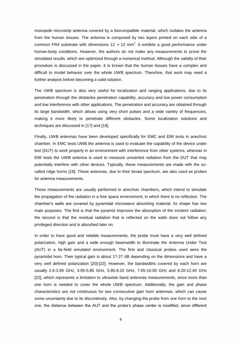
monopole microstrip antenna covered by a biocompatible material, which isolates the antenna
from the human tissues. The antenna is composed by two layers printed on each side of a
common FR4 substrate with dimensions 12 × 12 mm2. It exhibits a good performance under
human-body conditions. However, the authors do not make any measurements to prove the
simulated results, which are optimized through a numerical method. Although the validity of their
procedure is discussed in the paper, it is known that the human tissues have a complex and
difficult to model behavior over the whole UWB spectrum. Therefore, that work may need a
further analysis before becoming a valid solution.
The UWB spectrum is also very useful for localization and ranging applications, due to its
penetration through the obstacles penetration capability, accuracy and low power consumption
and low interference with other applications. The penetration and accuracy are obtained through
its large bandwidth, which allows using very short pulses and a wide variety of frequencies,
making it more likely to penetrate different obstacles. Some localization solutions and
techniques are discussed in [17] and [18].
Finally, UWB antennas have been developed specifically for EMC and EMI tests in anechoic
chamber. In EMC tests UWB the antenna is used to evaluate the capability of the device under
test (DUT) to work properly in an environment with interference from other systems, whereas in
EMI tests the UWB antenna is used to measure unwanted radiation from the DUT that may
potentially interfere with other devices. Typically, these measurements are made with the so-
called ridge horns [19]. These antennas, due to their broad spectrum, are also used as probes
for antenna measurements.
These measurements are usually performed in anechoic chambers, which intend to simulate
the propagation of the radiation in a free space environment, in which there is no reflection. The
chamber’s walls are covered by pyramidal microwave absorbing material. Its shape has two
main purposes. The first is that the pyramid improves the absorption of the incident radiation;
the second is that the residual radiation that is reflected on the walls does not follow any
privileged direction and is absorbed later on.
In order to have good and reliable measurements, the probe must have a very well defined
polarization, high gain and a wide enough beamwidth to illuminate the Antenna Under Test
(AUT) in a far-field emulated environment. The first and classical probes used were the
pyramidal horn. Their typical gain is about 17-27 dB depending on the dimensions and have a
very well defined polarization [20]-[22]. However, the bandwidths covered by each horn are
usually 2.6-3.95 GHz, 3.95-5.85 GHz, 5.85-8.20 GHz, 7.05-10.00 GHz and 8.20-12.40 GHz
[22], which represents a limitation to ultrawide band antennas measurements, since more than
one horn is needed to cover the whole UWB spectrum. Additionally, the gain and phase
characteristics are not continuous for two consecutive gain horn antennas, which can cause
some uncertainty due to its discontinuity. Also, by changing the probe from one horn to the next
one, the distance between the AUT and the probe’s phase center is modified, since different

5
bandwidth probes have different sizes, and this distance must remain as stable as possible in
order not to change the measurements results.
The ridge horns are used to overcome the problem of the limited bandwidth of the classical
horn. This antenna adds ridges to the classical horn’s design, in order to cover a wider band.
Differently sized ridge horns can be manufactured in order to cover different frequency bands.
The most common are typically the 0.8-12 GHz, 1-18 GHz or even 18-40 GHz [19], [23]. Since
the goal of this thesis is to cover the UWB spectrum, this analysis focuses mainly on the second
type of ridge horn.
The ridge horns are generally divided into two categories, double- and quad-ridge horns,
depending on the number of ridges they have. The first usually contains only one feed port and
is suitable to measure one linear polarization at a time [24]. On the contrary, the quad-ridge
horns are commonly used with two feed ports, in order to provide measurements in two
orthogonal polarizations [25].
Each category can then be sub-categorized by type of sidewalls: dielectric or metallic grid
sidewalls and open boundary ridge horn. A benchmark study of double-ridge horn is performed
in [26]. The authors verify that the dielectric and metallic grid sidewalls double-ridge horns suffer
from polarization deterioration, since they present a pattern split-up into four lobes at higher
frequencies. Nevertheless, the metallic double-ridge horn already exhibits a considerable
improvement, when compared to the dielectric grid sidewalls one. The open boundary double-
ridge horn reveals no pattern breakup. However, it has low gain at lower frequencies [26].
Despite presenting these drawbacks, the ridge horns are also difficult to manufacture and to
assembly, since if any gap is left between two (or more) assembling parts it produces higher
order propagation modes and new resonance frequencies that deteriorate the antenna
performance [26]. Furthermore, these antennas have low gain in the UWB frequency spectrum
and the beamwidth is considerably different in the E- and H- planes, which are important
required features for any probe antenna [26]. Besides this, they are expensive and sometimes
are heavy, weighting up to almost 2 kg alone [23].
6
1.3. XETS description
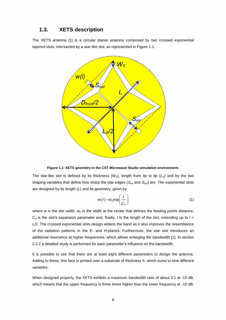
The XETS antenna [1] is a circular planar antenna composed by two crossed exponential
tapered slots, intersected by a star-like slot, as represented in Figure 1.1.
Figure 1.1: XETS geometry in the CST Microwave Studio simulation environment.
The star-like slot is defined by its thickness (WS), length from tip to tip (LS) and by the two
shaping variables that define how sharp the star edges (Sint and Sext) are. The exponential slots
are designed by its length (L) and its geometry, given by
0
0
expl
w l wC
(1)
where w is the slot width, w0 is the width at the center that defines the feeding points distance,
C0 is the slot’s expansion parameter and, finally, l is the length of the slot, extending up to l =
L/2. The crossed exponential slots design widens the band as it also improves the resemblance
of the radiation patterns in the E- and H-planes. Furthermore, the star slot introduces an
additional resonance at higher frequencies, which allows enlarging the bandwidth [1]. In section
2.2.2 a detailed study is performed for each parameter’s influence on the bandwidth.
It is possible to see that there are at least eight different parameters to design the antenna.
Adding to these, this face is printed over a substrate of thickness h, which sums to nine different
variables.
When designed properly, the XETS exhibits a maximum bandwidth ratio of about 3:1 at -10 dB,
which means that the upper frequency is three times higher than the lower frequency at -10 dB.
w(l)
WS
L
Sint
Sext
Dfront/2
LS/2

7
Therefore, this antenna is very good to cover the UWB band from 3.18 GHz up to 10.6 GHz, as
seen in [1].
The XETS radiation pattern remains quite stable with frequency and is symmetric in the E- and
H-planes, since the antenna has two symmetry planes. Note that the symmetry is only verified if
the antenna is fed by a discrete port, otherwise the feeding cable distorts the radiation pattern in
the E-plane, since it ruins the symmetry. Furthermore, the XETS radiation pattern has a toroidal
shape, similar to the radiation pattern of the dipole. Another property of this antenna is that it
has a very well defined polarization. Also, the phase center is localized in the antenna’s
geometrical center and does not move with the frequency. The XETS is proper for pulse-based
systems, since it preserves the transmitted pulses shape quite well, allowing to reach high data
rates.
Figure 1.2: XETS feeding scheme in CST with discrete port feeding detail.
The feeding can be made through two of the diamond-shaped “petals” in the front face (Figure
1.1) or, if convenient, it is possible to add two “petals” in the back face and feed the antenna
through there. The E-plane corresponds to φ = 0˚, whereas the H-plane corresponds to φ = 90˚,
assuming that the antenna is fed as in Figure 1.2. Two different feed configurations have been
tested: coaxial cable, as in [1] and [2] and microstrip line feeding, as in [3]. Since the antenna
has a balanced configuration, the use of an unbalanced feed, as is the case of the coaxial
cable, should require a structure to make the appropriate transition between the antenna and
the cable. Such structure is called BALUN. However, since the cables used in [1] and [2] are
very thin it was considered that there was no need for a BALUN. This could be assumed
because the cable is so thin that the impedance of the outer conductor tends to be very high
and, therefore, the currents flowing outside the cable are minimal, excluding the need of a
BALUN. Nevertheless, the coaxial cable has consequences in the antenna’s performance, since
the cable starts to radiate by itself, which moves the phase center and increases the cross
polarization level.
θ
Φ=0˚ Φ

8
1.4. XETS applications
The XETS was first designed as a feed for an integrated lens antenna for mm-wave applications
[2]. The authors propose an antenna integrated with a MACOR elliptical lens for operation
between 35 and 70 GHz. The XETS size is 1.7 mm, which radiates directly into the lens. A
XETS is also presented for the band 1.4-4 GHz frequency band with a diameter of 70 mm,
radiating into the air and fed by a coaxial cable. The antenna is printed on a single sided Duroid
5880 substrate with permittivity εr = 2.2, loss tangent tan(δ) = 0.0009 and thickness h = 10 mil
(0.254 mm). In both cases, the measurements have shown a good performance within the
band.
This paper motivated another application, already mentioned earlier [1]. Here, the authors
present a XETS to cover the whole UWB spectrum. The XETS diameter is 35 mm, which is fed
by a coaxial cable. The antenna was fabricated using the same Duroid 5880 substrate as before
(εr = 2.2, tan(δ) = 0.0009 and h = 10 mil). The results exhibit a very good performance within the
band. The polarization is very well defined and the phase is very stable around boresight. The
directivity is approximately 4 dBi at the lower frequencies of the UWB spectrum and 6 dBi at the
higher ones. The efficiency has been predicted to be between 90% and 97% across the
bandwidth. Also, the pulse fidelity parameter (a measure of the antenna’s capability of
preserving the shape of the transmitted pulse) [1] has been proven to be approximately 90%
and, in the worst case scenario, of about 70%.
In [5] it is shown that it is possible to reject the WLAN operation band, by re-shaping the
antenna’s geometry. The authors verify that by adding additional slots in the front “petals” it is
possible to create a notch around 5.5 GHz. The measurements illustrate that the antenna’s
characteristics outside the rejected band remain reasonably unmodified.
Furthermore, a variant of the XETS was developed that is adequate for WLAN access points
[3]. This application is suitable for base stations, since it operates from 2.5 GHz to 4.8 GHz. It is
composed by an optimized XETS and by a back cavity with a squared mesh printed on FR4
substrate (εr = 4.9, tan(δ) = 0.025 and hFR4 = 1.6 mm), which increases the front-to-back ratio
although at the cost of reducing the band. The XETS is fed through a microstrip line, welded on
the back “petals”. The overall dimensions are 57 × 57 × 21 mm3. The measurements show a
very good performance over the whole bandwidth. The cross-polarization level is below -20 dB.
The authors confirmed that this design exhibited low coupling to adjacent elements, which made
it very suitable to Multiple Input Multiple Output (MIMO) systems [4]. Therefore, a four element
array was fabricated with overall dimensions of 114 × 114 × 21 mm3. This solution offers a
bandwidth that extends from 2.4 GHz up to 4.8 GHz, in which the mutual coupling between two
XETS is about -25 dB.
Finally, in [6] a new solution is discussed for localization and identification using the XETS
antenna integrated with a Radio Frequency Identification (RFID) chip, resulting in a hybrid

9
antenna. It consists of a 80 × 44 mm2 Duroid 5880 substrate (εr = 2.2, tan(δ) = 0.0009 and h =
0.254 mm) in which were printed a RFID tag and a XETS on each side. The RFID tag enables
the antenna to be activated by an Ultra High Frequency (UHF) signal and respond with a short
UWB pulse that improves the system’s localization accuracy. The results show that the average
position error is in the order of 2 cm reaching 6.5 cm in the worst case scenario. Also, when
compared to UWB commercial solutions, the hybrid antenna exhibit slightly better results.
10
1.5. Thesis structure
This thesis is organized in three chapters that concern to the XETS design, applications and
final remarks.
Chapter 2 presents the XETS analytical model design, which allows designing the antenna
automatically. It starts by introducing the methodology that is followed along the work. The
methodology explains that it is worth studying first the antenna it is necessary to first study the
antenna without substrate so it can be added afterwards and analyze its effect on the antenna
performance. As a result of this strategy, Chapter 2 is sub-divided into two sections, one
considering that the XETS is self-sustained in the air and in the other section the substrate is
taken into account. At the end of each sub-section some examples are discussed.
Two new applications are presented in Chapter 3, in which the XETS antenna is designed
through the expressions determined in Chapter 2. The first is an anechoic chamber probe with
UWB characteristics that takes advantage of the XETS features, for use in UWB antenna
measurements. The second application is a human-body implantable antenna. This application
is motivated by the need to access very fast to important medical data (e.g. health information
about a patient) in emergency scenarios. This can be achieved by storing data in a flash
memory that is integrated in the implantable antenna, which can be read by scanning the area
with an external antenna at a short distance.
Finally, in Chapter 4 the main conclusions are drawn.
11
2. XETS design
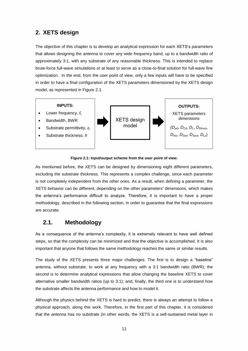
The objective of this chapter is to develop an analytical expression for each XETS’s parameters
that allows designing the antenna to cover any wide frequency band, up to a bandwidth ratio of
approximately 3:1, with any substrate of any reasonable thickness. This is intended to replace
brute-force full-wave simulations or at least to serve as a close-to-final solution for full-wave fine
optimization. In the end, from the user point of view, only a few inputs will have to be specified
in order to have a final configuration of the XETS parameters dimensioned by the XETS design
model, as represented in Figure 2.1.
Figure 2.1: Input/output scheme from the user point of view.
As mentioned before, the XETS can be designed by dimensioning eight different parameters,
excluding the substrate thickness. This represents a complex challenge, since each parameter
is not completely independent from the other ones. As a result, when defining a parameter, the
XETS behavior can be different, depending on the other parameters’ dimensions, which makes
the antenna’s performance difficult to analyze. Therefore, it is important to have a proper
methodology, described in the following section, in order to guarantee that the final expressions
are accurate.
2.1. Methodology
As a consequence of the antenna’s complexity, it is extremely relevant to have well defined
steps, so that the complexity can be minimized and that the objective is accomplished. It is also
important that anyone that follows the same methodology reaches the same or similar results.
The study of the XETS presents three major challenges. The first is to design a “baseline”
antenna, without substrate, to work at any frequency with a 3:1 bandwidth ratio (BWR); the
second is to determine analytical expressions that allow changing the baseline XETS to cover
alternative smaller bandwidth ratios (up to 3:1); and, finally, the third one is to understand how
the substrate affects the antenna performance and how to model it.
Although the physics behind the XETS is hard to predict, there is always an attempt to follow a
physical approach, along this work. Therefore, in the first part of this chapter, it is considered
that the antenna has no substrate (in other words, the XETS is a self-sustained metal layer in
XETS design model
INPUTS:
Lower frequency, fL
Bandwidth, BWR
Substrate permittivity, εr
Substrate thickness, h
OUTPUTS:
XETS parameters dimensions
(Dw0, DC0, DL, DDfront,
DWs, DSint, DSext, DLs)
12
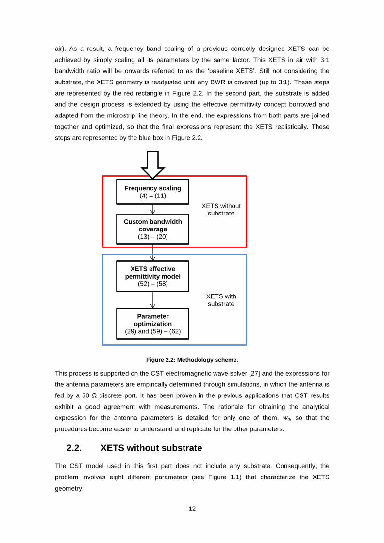
air). As a result, a frequency band scaling of a previous correctly designed XETS can be
achieved by simply scaling all its parameters by the same factor. This XETS in air with 3:1
bandwidth ratio will be onwards referred to as the ‘baseline XETS’. Still not considering the
substrate, the XETS geometry is readjusted until any BWR is covered (up to 3:1). These steps
are represented by the red rectangle in Figure 2.2. In the second part, the substrate is added
and the design process is extended by using the effective permittivity concept borrowed and
adapted from the microstrip line theory. In the end, the expressions from both parts are joined
together and optimized, so that the final expressions represent the XETS realistically. These
steps are represented by the blue box in Figure 2.2.
Figure 2.2: Methodology scheme.
This process is supported on the CST electromagnetic wave solver [27] and the expressions for
the antenna parameters are empirically determined through simulations, in which the antenna is
fed by a 50 Ω discrete port. It has been proven in the previous applications that CST results
exhibit a good agreement with measurements. The rationale for obtaining the analytical
expression for the antenna parameters is detailed for only one of them, w0, so that the
procedures become easier to understand and replicate for the other parameters.
2.2. XETS without substrate
The CST model used in this first part does not include any substrate. Consequently, the
problem involves eight different parameters (see Figure 1.1) that characterize the XETS
geometry.
Frequency scaling (4) – (11)
Custom bandwidth coverage (13) – (20)
XETS effective permittivity model
(52) – (58)
Parameter optimization
(29) and (59) – (62)
XETS without substrate
XETS with substrate

13
2.2.1. ‘Baseline XETS’: frequency scaling
The first step is to dimension the XETS to work at any frequency range with 3:1 bandwidth ratio.
To accomplish this, we start from the full-wave simulator design of a XETS without substrate
that works in a specific frequency band with 3:1 BWR. Extension for other frequency limits
complying with the 3:1 BWR is obtained by linear scaling, inversely proportional to the
frequency. Thus, it is assumed that the parameters’ dimensioning rule is
L
KD
f (2)
where D represents any of the parameter’s dimension in millimeter of the full-wave designed
XETS, K is a constant that defines the linear slope and fL is the desired lower frequency limit in
GHz. Since the frequency bandwidth is very wide, the convention in this work is that the XETS
bandwidth is defined by the lower frequency fL at -10 dB input reflection level and by the
bandwidth ratio U LBWR f f (fU is the upper frequency at -10 dB input reflection level).
The scaling factor K should be different for every antenna’s parameter. It can be established
from (2) by replacing fL and D for a known baseline XETS:
0 0LK D f (3)
where D0 is the baseline antenna’s parameter dimension (in millimeter) at frequency fL0 (in
GHz), which is the lower frequency at -10 dB as previously mentioned. This expression must be
applied to every variable, resulting in a total of eight different expressions.
The XETS reference antenna used for this purpose was dimensioned using CST full-wave
simulation to work from 3.30 GHz up to 10.42 GHz1. The corresponding dimensions and the
reflection coefficient curve are presented in Table 2.1 and Figure 2.3, respectively.
Table 2.1: XETS variables dimensions in millimeters designed for the band 3.3-10.42 GHz without substrate.
w0 C0 L Dfront WS Sint Sext LS
0.195 8.1 28.9 41.5 2.9 1.9 -1.45 35.8
Figure 2.3: a) XETS CST model; b) reflection coefficient of the XETS designed for the 3.3-10.42 GHz without substrate.
1 This corresponds to the FCC definition of the UWB spectrum.
b) a)
14
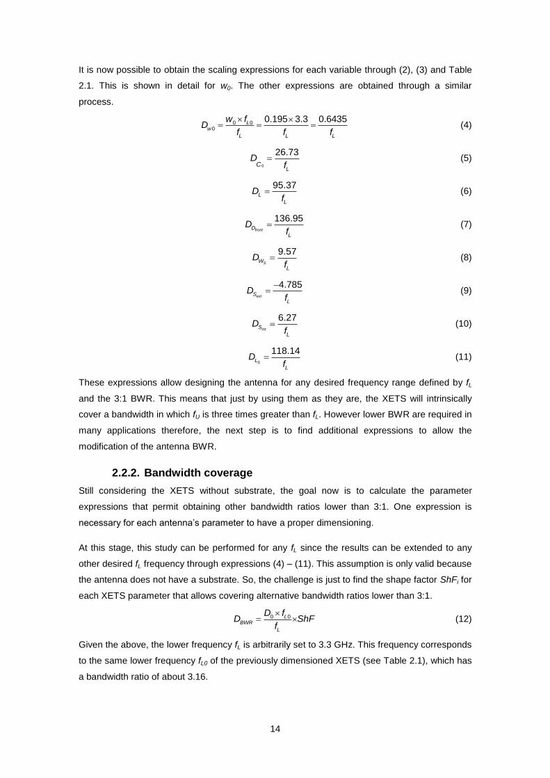
It is now possible to obtain the scaling expressions for each variable through (2), (3) and Table
2.1. This is shown in detail for w0. The other expressions are obtained through a similar
process.
0 00
0.195 3.3 0.6435Lw
L L L
w fD
f f f
(4)
0
26.73
LC
Df
(5)
95.37
L
L
Df
(6)
136.95
frontD
L
Df
(7)
9.57
SW
L
Df
(8)
4.785
extS
L
Df
(9)
6.27
intS
L
Df
(10)
118.14
SL
L
Df
(11)
These expressions allow designing the antenna for any desired frequency range defined by fL
and the 3:1 BWR. This means that just by using them as they are, the XETS will intrinsically
cover a bandwidth in which fU is three times greater than fL. However lower BWR are required in
many applications therefore, the next step is to find additional expressions to allow the
modification of the antenna BWR.
2.2.2. Bandwidth coverage
Still considering the XETS without substrate, the goal now is to calculate the parameter
expressions that permit obtaining other bandwidth ratios lower than 3:1. One expression is
necessary for each antenna’s parameter to have a proper dimensioning.
At this stage, this study can be performed for any fL since the results can be extended to any
other desired fL frequency through expressions (4) – (11). This assumption is only valid because
the antenna does not have a substrate. So, the challenge is just to find the shape factor ShFi for
each XETS parameter that allows covering alternative bandwidth ratios lower than 3:1.
0 0 LBWR
L
D fD ShF
f
(12)
Given the above, the lower frequency fL is arbitrarily set to 3.3 GHz. This frequency corresponds
to the same lower frequency fL0 of the previously dimensioned XETS (see Table 2.1), which has
a bandwidth ratio of about 3.16.
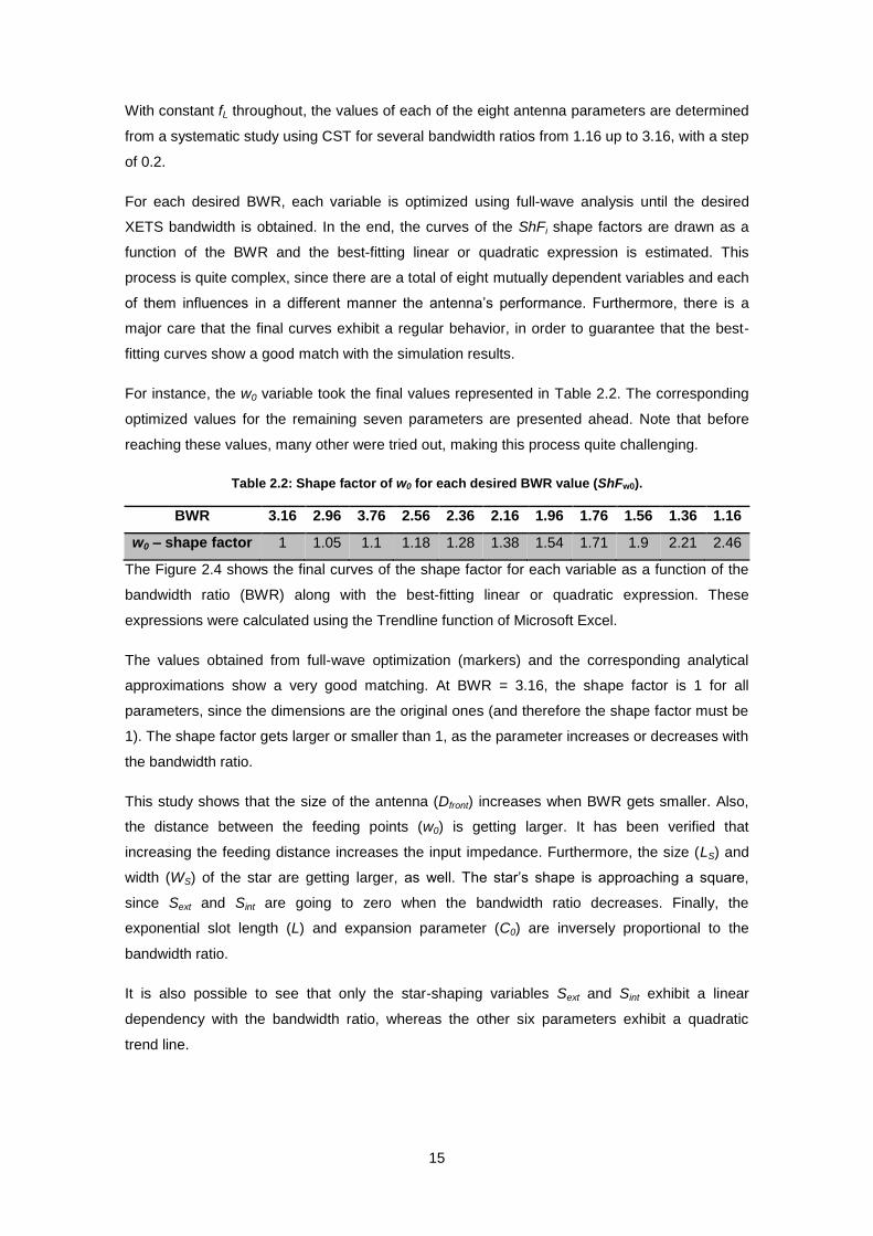
15
With constant fL throughout, the values of each of the eight antenna parameters are determined
from a systematic study using CST for several bandwidth ratios from 1.16 up to 3.16, with a step
of 0.2.
For each desired BWR, each variable is optimized using full-wave analysis until the desired
XETS bandwidth is obtained. In the end, the curves of the ShFi shape factors are drawn as a
function of the BWR and the best-fitting linear or quadratic expression is estimated. This
process is quite complex, since there are a total of eight mutually dependent variables and each
of them influences in a different manner the antenna’s performance. Furthermore, there is a
major care that the final curves exhibit a regular behavior, in order to guarantee that the best-
fitting curves show a good match with the simulation results.
For instance, the w0 variable took the final values represented in Table 2.2. The corresponding
optimized values for the remaining seven parameters are presented ahead. Note that before
reaching these values, many other were tried out, making this process quite challenging.
Table 2.2: Shape factor of w0 for each desired BWR value (ShFw0).
BWR 3.16 2.96 3.76 2.56 2.36 2.16 1.96 1.76 1.56 1.36 1.16
w0 – shape factor 1 1.05 1.1 1.18 1.28 1.38 1.54 1.71 1.9 2.21 2.46
The Figure 2.4 shows the final curves of the shape factor for each variable as a function of the
bandwidth ratio (BWR) along with the best-fitting linear or quadratic expression. These
expressions were calculated using the Trendline function of Microsoft Excel.
The values obtained from full-wave optimization (markers) and the corresponding analytical
approximations show a very good matching. At BWR = 3.16, the shape factor is 1 for all
parameters, since the dimensions are the original ones (and therefore the shape factor must be
1). The shape factor gets larger or smaller than 1, as the parameter increases or decreases with
the bandwidth ratio.
This study shows that the size of the antenna (Dfront) increases when BWR gets smaller. Also,
the distance between the feeding points (w0) is getting larger. It has been verified that
increasing the feeding distance increases the input impedance. Furthermore, the size (LS) and
width (WS) of the star are getting larger, as well. The star’s shape is approaching a square,
since Sext and Sint are going to zero when the bandwidth ratio decreases. Finally, the
exponential slot length (L) and expansion parameter (C0) are inversely proportional to the
bandwidth ratio.
It is also possible to see that only the star-shaping variables Sext and Sint exhibit a linear
dependency with the bandwidth ratio, whereas the other six parameters exhibit a quadratic
trend line.

16
Figure 2.4: Shape factor for each antenna parameter from full-wave simulation (marker) and the corresponding best-fitting quadratic or linear curve and expression.
Although these expressions are the best-fitting ones, the shape factor at BWR = 3.16 is not
exactly 1, as it should be, because there is a residual error associated with the estimation.
Therefore, the expressions are forced to 1 at BWR = 3.16, simply by adding a constant. For w0
the constant is ‒0.021, resulting in
0
2
2
0.3332 2.1363 4.4447 0.021
0.3332 2.1363 4.4237wShF BWR BWR
BWR BWR
(13)
Similarly for the remaining parameters
0
20.0379 0.038 1.2588CShF BWR BWR (14)
20.1901 1.4808 3.7806
LShF BWR BWR (15)
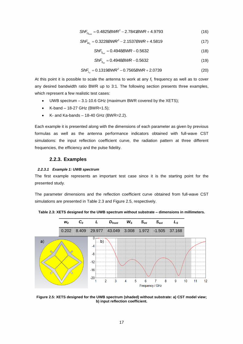
17
20.4825 2.7841 4.9793frontDShF BWR BWR (16)
20.3228 2.1537 4.5819SWShF BWR BWR (17)
0.4948 0.5632extSShF BWR (18)
0.4948 0.5632intSShF BWR (19)
20.1319 0.7565 2.0739SLShF BWR BWR (20)
At this point it is possible to scale the antenna to work at any fL frequency as well as to cover
any desired bandwidth ratio BWR up to 3:1. The following section presents three examples,
which represent a few realistic test cases:
UWB spectrum – 3.1-10.6 GHz (maximum BWR covered by the XETS);
K-band – 18-27 GHz (BWR=1.5);
K- and Ka-bands – 18-40 GHz (BWR=2.2).
Each example it is presented along with the dimensions of each parameter as given by previous
formulas as well as the antenna performance indicators obtained with full-wave CST
simulations: the input reflection coefficient curve, the radiation pattern at three different
frequencies, the efficiency and the pulse fidelity.
2.2.3. Examples
2.2.3.1 Example 1: UWB spectrum
The first example represents an important test case since it is the starting point for the
presented study.
The parameter dimensions and the reflection coefficient curve obtained from full-wave CST
simulations are presented in Table 2.3 and Figure 2.5, respectively.
Table 2.3: XETS designed for the UWB spectrum without substrate – dimensions in millimeters.
w0 C0 L Dfront WS Sint Sext LS
0.202 8.409 29.977 43.049 3.008 1.972 -1.505 37.168
Figure 2.5: XETS designed for the UWB spectrum (shaded) without substrate: a) CST model view; b) input reflection coefficient.

18
The reflection coefficient shows that the UWB spectrum is reasonably covered. The radiation
pattern and phase at 4 GHz, 7 GHz and 10 GHz are presented in Figure 2.6 -Figure 2.11.
Figure 2.6: XETS designed for the UWB spectrum without substrate- 3D view of the radiation pattern at 4 GHz.
Figure 2.7: XETS designed for the UWB spectrum without substrate - simulated radiation pattern and phase at 4 GHz in the E- (red) and H-planes (green): a) radiation pattern; b) phase.
Figure 2.8: XETS designed for the UWB without substrate spectrum - 3D view of the radiation pattern at 7 GHz.
Figure 2.9: XETS designed for the UWB spectrum without substrate - simulated radiation pattern and phase at 7 GHz in the E- (red) and H-planes (green): a) radiation pattern; b) phase.
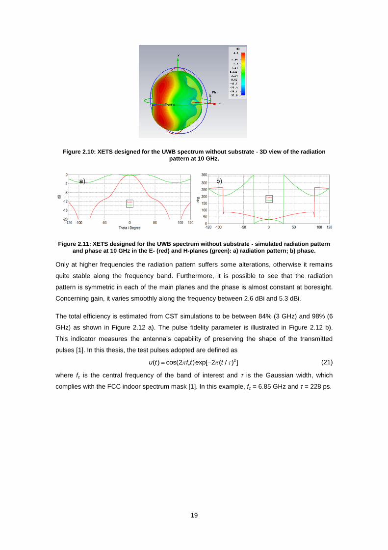
19
Figure 2.10: XETS designed for the UWB spectrum without substrate - 3D view of the radiation pattern at 10 GHz.
Figure 2.11: XETS designed for the UWB spectrum without substrate - simulated radiation pattern and phase at 10 GHz in the E- (red) and H-planes (green): a) radiation pattern; b) phase.
Only at higher frequencies the radiation pattern suffers some alterations, otherwise it remains
quite stable along the frequency band. Furthermore, it is possible to see that the radiation
pattern is symmetric in each of the main planes and the phase is almost constant at boresight.
Concerning gain, it varies smoothly along the frequency between 2.6 dBi and 5.3 dBi.
The total efficiency is estimated from CST simulations to be between 84% (3 GHz) and 98% (6
GHz) as shown in Figure 2.12 a). The pulse fidelity parameter is illustrated in Figure 2.12 b).
This indicator measures the antenna’s capability of preserving the shape of the transmitted
pulses [1]. In this thesis, the test pulses adopted are defined as
2( ) cos(2 )exp[ 2 ( / ) ]cu t f t t (21)
where fc is the central frequency of the band of interest and τ is the Gaussian width, which
complies with the FCC indoor spectrum mask [1]. In this example, fc = 6.85 GHz and τ = 228 ps.

20
Figure 2.12: XETS designed for UWB spectrum without substrate: a) total efficiency; b) fidelity over the solid angle. The radial angle is theta and the polar angle is phi.
Overall the XETS practically does not distort the pulses, since its fidelity varies between 95%
and 98%. Once again, due to the antenna’s symmetry, the fidelity also has two symmetry
planes. The values of about 95% around θ = 90˚ and φ = 90˚ and 270˚ are a consequence of
the nulls in the radiation pattern in those directions.
2.2.3.2 Example 2: K-band
The second example is intended to cover the K-band (18-27 GHz with BWR = 1.5). The
antenna parameter dimensions, calculated from the expressions determined earlier, and the
corresponding reflection coefficient obtained from full-wave CST simulation are presented in
Table 2.4 and Figure 2.13, respectively.
Table 2.4: XETS designed for the K-band without substrate - dimensions in millimeters.
w0 C0 L Dfront WS Sint Sext LS
0.070 1.827 10.528 14.370 1.105 0.062 -0.048 8.112
Figure 2.13: XETS designed for the K-band (shaded) without substrate: a) CST model view; b) input reflection coefficient.
Although the reflection coefficient is a bit shifted to higher frequencies, there is a good coverage
of the K-band. The radiation pattern and phase at 19 GHz, 23 GHz and 27 GHz are shown in
Figure 2.14 - Figure 2.19.
a)
b)
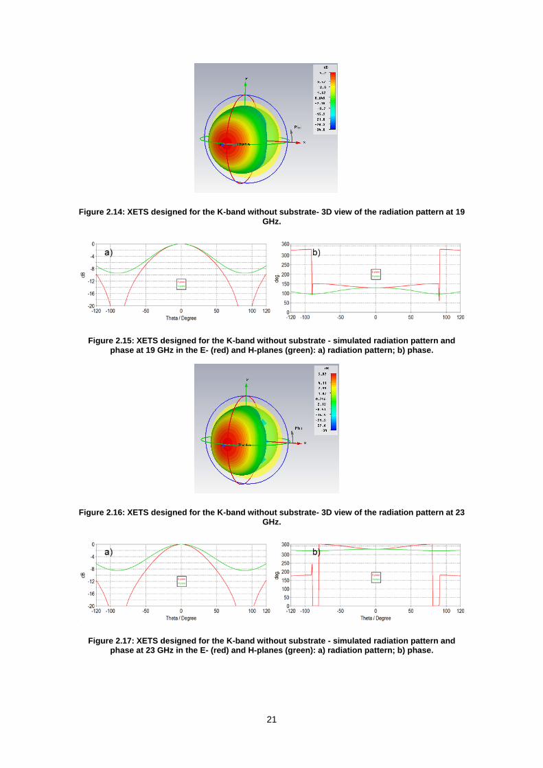
21
Figure 2.14: XETS designed for the K-band without substrate- 3D view of the radiation pattern at 19 GHz.
Figure 2.15: XETS designed for the K-band without substrate - simulated radiation pattern and phase at 19 GHz in the E- (red) and H-planes (green): a) radiation pattern; b) phase.
Figure 2.16: XETS designed for the K-band without substrate- 3D view of the radiation pattern at 23 GHz.
Figure 2.17: XETS designed for the K-band without substrate - simulated radiation pattern and phase at 23 GHz in the E- (red) and H-planes (green): a) radiation pattern; b) phase.

22
Figure 2.18: XETS designed for the K-band without substrate- 3D view of the radiation pattern at 27 GHz.
Figure 2.19: XETS designed for the K-band without substrate - simulated radiation pattern and phase at 27 GHz in the E- (red) and H-planes (green): a) radiation pattern; b) phase.
It is observed that the radiation pattern remains relatively unchanged along the band and
symmetric in both planes. Furthermore, the phase near boresight is fairly constant and the gain
varies between 4.1 dBi and 6 dBi.
The efficiency is estimated from CST simulations to be around 86% at 18 GHz and 98% at 24
GHz, as illustrated in Figure 2.20 a). The pulse fidelity is represented in Figure 2.20 b), using a
test pulse of the form (21) with fc = 22.5 GHz and τ = 270 ps. The values range from 80% to
100%, which is worse than in the previous example but still reasonable values with average
around 95%. As in the previous example, the minimum values occur at the nulls of the radiation
pattern.
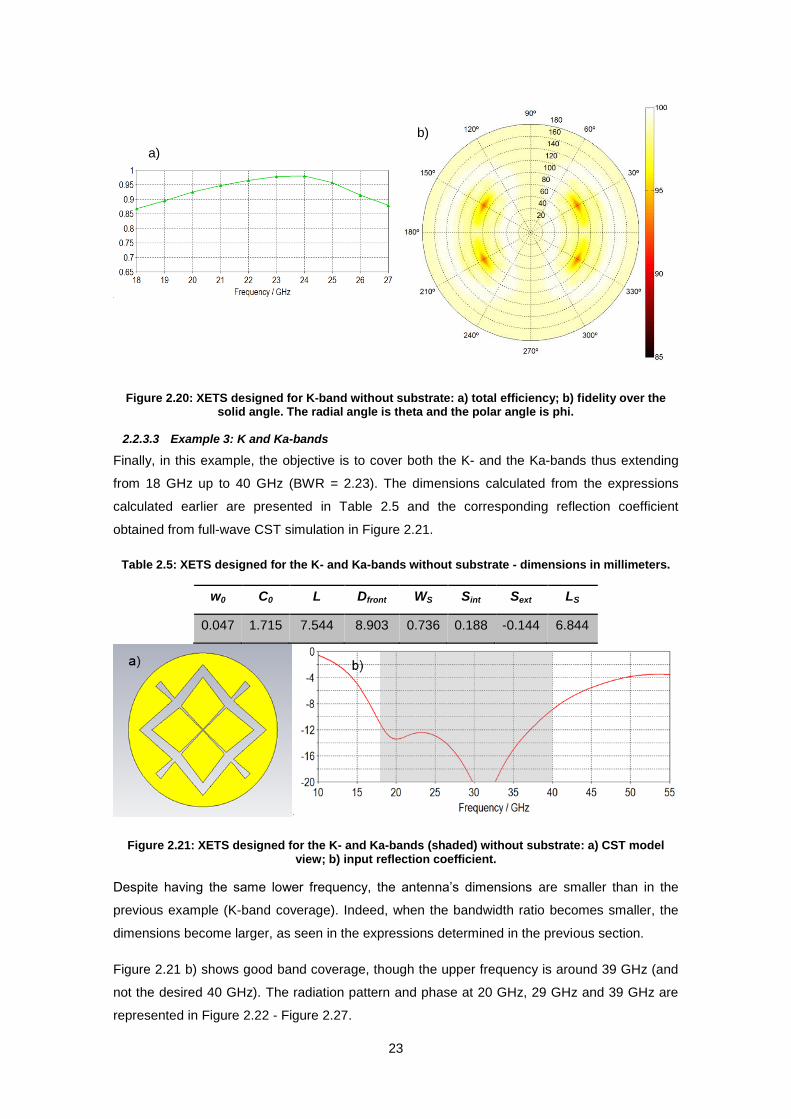
23
Figure 2.20: XETS designed for K-band without substrate: a) total efficiency; b) fidelity over the solid angle. The radial angle is theta and the polar angle is phi.
2.2.3.3 Example 3: K and Ka-bands
Finally, in this example, the objective is to cover both the K- and the Ka-bands thus extending
from 18 GHz up to 40 GHz (BWR = 2.23). The dimensions calculated from the expressions
calculated earlier are presented in Table 2.5 and the corresponding reflection coefficient
obtained from full-wave CST simulation in Figure 2.21.
Table 2.5: XETS designed for the K- and Ka-bands without substrate - dimensions in millimeters.
w0 C0 L Dfront WS Sint Sext LS
0.047 1.715 7.544 8.903 0.736 0.188 -0.144 6.844
Figure 2.21: XETS designed for the K- and Ka-bands (shaded) without substrate: a) CST model view; b) input reflection coefficient.
Despite having the same lower frequency, the antenna’s dimensions are smaller than in the
previous example (K-band coverage). Indeed, when the bandwidth ratio becomes smaller, the
dimensions become larger, as seen in the expressions determined in the previous section.
Figure 2.21 b) shows good band coverage, though the upper frequency is around 39 GHz (and
not the desired 40 GHz). The radiation pattern and phase at 20 GHz, 29 GHz and 39 GHz are
represented in Figure 2.22 - Figure 2.27.
a)
b)
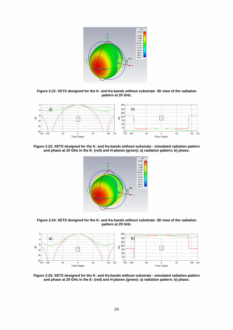
24
Figure 2.22: XETS designed for the K- and Ka-bands without substrate- 3D view of the radiation pattern at 20 GHz.
Figure 2.23: XETS designed for the K- and Ka-bands without substrate - simulated radiation pattern and phase at 20 GHz in the E- (red) and H-planes (green): a) radiation pattern; b) phase.
Figure 2.24: XETS designed for the K- and Ka-bands without substrate- 3D view of the radiation pattern at 29 GHz.
Figure 2.25: XETS designed for the K- and Ka-bands without substrate - simulated radiation pattern and phase at 29 GHz in the E- (red) and H-planes (green): a) radiation pattern; b) phase.
a) b)

25
Figure 2.26: XETS designed for the K- and Ka-bands without substrate- 3D view of the radiation pattern at 39 GHz.
Figure 2.27: XETS designed for the K- and Ka-bands without substrate - simulated radiation pattern and phase at 39 GHz in the E- (red) and H-planes (green): a) radiation pattern; b) phase.
Once again, the radiation pattern is symmetric in both planes and it is very stable along the
frequency. Also, the phase is quite smooth near boresight. Furthermore, the gain should be
between 3.3 dBi and 6.1 dBi. The total efficiency ranges between 86% and 98%, as presented
in Figure 2.28 a). Concerning pulse fidelity, it is shown in Figure 2.28 that the minimum and
maximum values are approximately 95% and 98%, respectively. The fidelity is very good since
the radiation pattern is very stable along the spectrum while the phase center that does not
suffer any major modification. The test pulse is defined as in (21) with fc = 29 GHz and τ = 110
ps.
Figure 2.28: XETS designed for K- and Ka-bands without substrate: a) total efficiency; b) fidelity over the solid angle. The radial angle is theta and the polar angle is phi.
b) a)

26
2.3. Effective permittivity model
The expressions determined so far do not take into account the effect of the substrate. Thus,
the next objective is to study how to extend the previous expressions for the general case
where the XETS includes a dielectric substrate.
One bold approach to include the dielectric substrate in the antenna design equations is to
explore the possibility of adapting the well-known effective permittivity concept used for
microstrip lines. The classical microstrip line is represented in Figure 2.29. The substrate has
height hms and relative permittivity εr, whereas the microstrip line has width Wms.
Figure 2.29: Classical microstrip transmission line geometry (based on [28]).
A classical microstrip line propagates quasi-TEM modes that have vestigial longitudinal
component of the fields, since the fields are not restricted to the substrate. Indeed, some of the
fields propagate through the air (or any other medium surrounding the microstrip line). The
microstrip line theory states that propagation constant in the microstrip line configuration of
Figure 2.29 is very well approximated by the propagation constant in the equivalent structure of
Figure 2.30 where an infinite homogeneous dielectric medium with an appropriately calculated
effective permittivity εeff contains all the fields lines. In other words, any microstrip line can be
dimensioned considering a simpler formulation for an infinite homogenous medium with
effective permittivity (εeff) that embeds the transmission line [28], as in Figure 2.30.
Figure 2.30: Equivalent geometry of the microstrip line with permittivity εeff (based on [28]).
Once the microstrip is surrounded by an infinite effective medium, then it is possible to linearly
scale the design to any frequency. It is also possible to scale it for any effective permittivity
value (provided that the appropriate relation between εr and εeff is found). So, the width of the
classical microstrip line with air substrate and the re-dimensioned microstrip line in the
equivalent medium are related as follows
hms
Wms
εr
εeff
hms
Wms
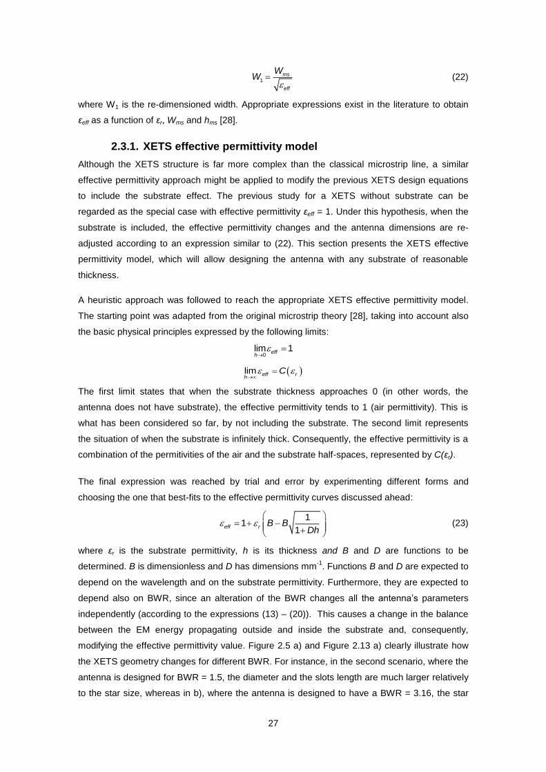
27
1ms
eff
WW (22)
where W1 is the re-dimensioned width. Appropriate expressions exist in the literature to obtain
εeff as a function of εr, Wms and hms [28].
2.3.1. XETS effective permittivity model
Although the XETS structure is far more complex than the classical microstrip line, a similar
effective permittivity approach might be applied to modify the previous XETS design equations
to include the substrate effect. The previous study for a XETS without substrate can be
regarded as the special case with effective permittivity εeff = 1. Under this hypothesis, when the
substrate is included, the effective permittivity changes and the antenna dimensions are re-
adjusted according to an expression similar to (22). This section presents the XETS effective
permittivity model, which will allow designing the antenna with any substrate of reasonable
thickness.
A heuristic approach was followed to reach the appropriate XETS effective permittivity model.
The starting point was adapted from the original microstrip theory [28], taking into account also
the basic physical principles expressed by the following limits:
0lim 1effh
lim eff rh
C
The first limit states that when the substrate thickness approaches 0 (in other words, the
antenna does not have substrate), the effective permittivity tends to 1 (air permittivity). This is
what has been considered so far, by not including the substrate. The second limit represents
the situation of when the substrate is infinitely thick. Consequently, the effective permittivity is a
combination of the permitivities of the air and the substrate half-spaces, represented by C(εr).
The final expression was reached by trial and error by experimenting different forms and
choosing the one that best-fits to the effective permittivity curves discussed ahead:
1
11
eff r B BDh
(23)
where εr is the substrate permittivity, h is its thickness and B and D are functions to be
determined. B is dimensionless and D has dimensions mm-1
. Functions B and D are expected to
depend on the wavelength and on the substrate permittivity. Furthermore, they are expected to
depend also on BWR, since an alteration of the BWR changes all the antenna’s parameters
independently (according to the expressions (13) – (20)). This causes a change in the balance
between the EM energy propagating outside and inside the substrate and, consequently,
modifying the effective permittivity value. Figure 2.5 a) and Figure 2.13 a) clearly illustrate how
the XETS geometry changes for different BWR. For instance, in the second scenario, where the
antenna is designed for BWR = 1.5, the diameter and the slots length are much larger relatively
to the star size, whereas in b), where the antenna is designed to have a BWR = 3.16, the star

28
size is comparable to the slots length and almost reaches the edge of the antenna. This
suggests that the effective permittivity must suffer modifications when the BWR changes.
Assuming that the effective permittivity concept is viable, the antenna can be re-designed
considering a similar expression to (22). Then, if DBL represents the dimension of any parameter
of the XETS without substrate and D1 is the corresponding dimension obtained from full-wave
simulations for the XETS with substrate, the effective permittivity value can be extracted from
2
1
BLeff
D
D
(24)
As will be shown ahead, some additional tuning steps will be added to this simple model in
order to reproduce correctly the complex nature of the XETS’s eight parameter dependency
with permittivity, frequency and BWR.
2.3.1.1 Study of B and D functions
From now on, the ratio 1 BLD D will be referred to as scale factor (ScF). As a result, (24) can be
re-written as
2
1.
( )eff
ScF (25)
Functions B and D can now be estimated from (25): the starting point is the XETS without
substrate, which is obtained with the previously determined expressions; then, the substrate is
added and the antenna’s parameters are scaled by the same factor until the XETS is working at
the same (lower) frequency checked by CST full-wave simulations. When this is accomplished it
is possible to calculate the effective permittivity and in principle B and D can be estimated.
However, as previously referred, B and D are also functions of other parameters, such as
substrate permittivity, wavelength and bandwidth ratio BWR. From this point on, B and D
expressions will be explicitly referred to as B(εr, BWR) and D(λL, εr, BWR), according to their
dependencies.
The referred dependence must be modeled by an analytical expression. Some methodology
must be defined to determine the B(εr, BWR) and D(λL, εr, BWR) dependency on each of the
parameters. This process involves full-wave simulations, in which the bandwidth ratio BWR,
substrate permittivity εr, frequency fL (note that λL is the wavelength corresponding to frequency
fL) and substrate thickness h are swept within practical limits according to the following steps:
Step 1 – Set the BWR;
Step 2 – Obtain the eight parameter values for the corresponding XETS without
substrate, calculated through the expressions determined for that purpose;
Step 3 – Within the desired BWR, sweep the substrate permittivity εr between 2.2 and
3.5;
Step 4 – For each εr, sweep the frequency from 1.564 GHz up to 32.675 GHz;

29
Step 5 – Within each frequency, sweep the substrate thickness between 0.01 mm and
3.175 mm;
Step 6 – Determine the ScF scale factor that optimizes the performance of the XETS
with substrate to work at the same fL frequency as the XETS without substrate,
including the w0 tuning that is discussed further ahead. Note that the same ScF scale
factor applies to the eight parameters defining the XETS;
Step 7 – Repeat the same procedure for different value of BWR.
These steps are represented by the red square in Figure 2.31.
Figure 2.31: Flowchart of the procedure followed in order to determine the XETS effective permittivity model.
The BWR is primarily set to 3.16 and then 2.16 and 1.56. The substrate permitivity and
thickness take consecutively standard values from the manufacturers [29]-[31]: hence εr = 2.2,
2.33, 2.94 and 3.5, whereas the thickness ranges between 0.127 mm and 3.175 mm [29]-[31].
Additional thickness values of 0.01 mm and 0.05 mm are also considered in order to increase
the accuracy of the effective permittivity model. Note that these values do not represent the
limits of the model. The model validity is discussed in section 2.3.3.
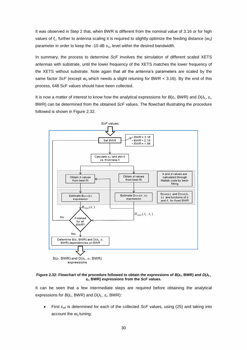
30
It was observed in Step 2 that, when BWR is different from the nominal value of 3.16 or for high
values of fL, further to antenna scaling it is required to slightly optimize the feeding distance (w0)
parameter in order to keep the -10 dB s11 level within the desired bandwidth.
In summary, the process to determine ScF involves the simulation of different scaled XETS
antennas with substrate, until the lower frequency of the XETS matches the lower frequency of
the XETS without substrate. Note again that all the antenna’s parameters are scaled by the
same factor ScF (except w0 which needs a slight retuning for BWR < 3.16). By the end of this
process, 648 ScF values should have been collected.
It is now a matter of interest to know how the analytical expressions for B(εr, BWR) and D(λL, εr,
BWR) can be determined from the obtained ScF values. The flowchart illustrating the procedure
followed is shown in Figure 2.32.
Figure 2.32: Flowchart of the procedure followed to obtain the expressions of B(εr, BWR) and D(λL, εr, BWR) expressions from the ScF values.
It can be seen that a few intermediate steps are required before obtaining the analytical
expressions for B(εr, BWR) and D(λL, εr, BWR):
First εeff is determined for each of the collected ScF values, using (25) and taking into
account the w0 tuning;
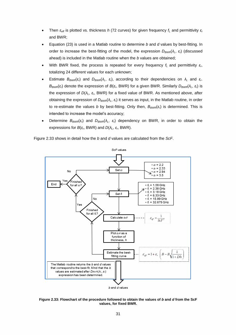
31
Then εeff is plotted vs. thickness h (72 curves) for given frequency fL and permittivity εr
and BWR;
Equation (23) is used in a Matlab routine to determine b and d values by best-fitting. In
order to increase the best-fitting of the model, the expression DBWR(λL, εr) (discussed
ahead) is included in the Matlab routine when the b values are obtained;
With BWR fixed, the process is repeated for every frequency fL and permittivity εr,
totalizing 24 different values for each unknown;
Estimate BBWR(εr) and DBWR(λL, εr), according to their dependencies on λL and εr.
BBWR(εr) denote the expression of B(εr, BWR) for a given BWR. Similarly DBWR(λL, εr) is
the expression of D(λL, εr, BWR) for a fixed value of BWR. As mentioned above, after
obtaining the expression of DBWR(λL, εr) it serves as input, in the Matlab routine, in order
to re-estimate the values b by best-fitting. Only then, BBWR(εr) is determined. This is
intended to increase the model’s accuracy;
Determine BBWR(εr) and DBWR(λL, εr) dependency on BWR, in order to obtain the
expressions for B(εr, BWR) and D(λL, εr, BWR).
Figure 2.33 shows in detail how the b and d values are calculated from the ScF.
Figure 2.33: Flowchart of the procedure followed to obtain the values of b and d from the ScF values, for fixed BWR.
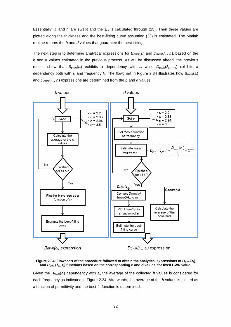
32
Essentially, εr and fL are swept and the εeff is calculated through (25). Then these values are
plotted along the thickness and the best-fitting curve assuming (23) is estimated. The Matlab
routine returns the b and d values that guarantee the best-fitting.
The next step is to determine analytical expressions for BBWR(εr) and DBWR(λL, εr), based on the
b and d values estimated in the previous process. As will be discussed ahead, the previous
results show that BBWR(εr) exhibits a dependency with εr while DBWR(λL, εr) exhibits a
dependency both with εr and frequency fL. The flowchart in Figure 2.34 illustrates how BBWR(εr)
and DBWR(λL, εr) expressions are determined from the b and d values.
Figure 2.34: Flowchart of the procedure followed to obtain the analytical expressions of BBWR(εr) and DBWR(λL, εr) functions based on the corresponding b and d values, for fixed BWR value.
Given the BBWR(εr) dependency with εr, the average of the collected b values is considered for
each frequency as indicated in Figure 2.34. Afterwards, the average of the b values is plotted as
a function of permittivity and the best-fit function is determined.
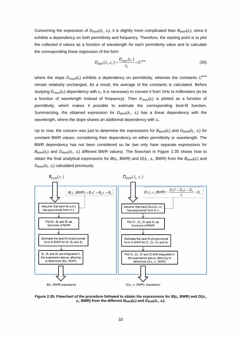
33
Concerning the expression of DBWR(λL, εr), it is slightly more complicated than BBWR(εr), since it
exhibits a dependency on both permittivity and frequency. Therefore, the starting point is to plot
the collected d values as a function of wavelength for each permittivity value and to calculate
the corresponding linear regression of the form
,( )
( )slope onst
BWR L r
r
L
DD C
(26)
where the slope Dslope(εr) exhibits a dependency on permittivity, whereas the constants Const
remain relatively unchanged. As a result, the average of the constants is calculated. Before
studying Dslope(εr) dependency with εr, it is necessary to convert it from GHz to millimeters (to be
a function of wavelength instead of frequency). Then Dslope(εr) is plotted as a function of
permittivity, which makes it possible to estimate the corresponding best-fit function.
Summarizing, the obtained expression for DBWR(λL, εr) has a linear dependency with the
wavelength, where the slope shares an additional dependency with εr.
Up to now, the concern was just to determine the expressions for BBWR(εr) and DBWR(λL, εr) for
constant BWR values, considering their dependency on either permittivity or wavelength. The
BWR dependency has not been considered so far (we only have separate expressions for
BBWR(εr) and DBWR(λL, εr) different BWR values). The flowchart in Figure 2.35 shows how to
obtain the final analytical expressions for B(εr, BWR) and D(λL, εr, BWR) from the BBWR(εr) and
DBWR(λL, εr) calculated previously.
Figure 2.35: Flowchart of the procedure followed to obtain the expressions for B(εr, BWR) and D(λL, εr, BWR) from the different BBWR(εr) and DBWR(λL, εr).
34
A practical approach is taken in order to determine the dependency of B(εr, BWR) and D(λL, εr,
BWR) on BWR. It is assumed that the expressions of BBWR(εr) and DBWR(λL, ε) are composed by
different coefficients (B1(BWR), B2(BWR) and B3(BWR); D1(BWR), D2(BWR), D3(BWR) and
D4(BWR)), as follows
2
1 2 3,r r rB BWR B BWR B BWR B BWR (27)
2
1 2 3
4, , .r r
L r
D BWR D BWR D BWRD BWR D BWR
(28)
The form of these expressions B(εr, BWR) and D(λL, εr, BWR) matches the form of the BBWR(εr)
and DBWR(λL, εr), respectively. Each of the BBWR(εr) and DBWR(λL, εr) expressions determined
before provides one coefficient Bi(BWR) (i = 1, 2 and 3) and Dj(BWR) (j = 1, 2, 3 and 4), which
are plotted vs. thickness h in a total of seven graphics (one for each coefficient). Then it is just
to calculate the best fitting curve for each of the coefficients and the dependency on BWR is
terminated. Note that the Bi(BWR) (i = 1, 2 and 3) and Dj(BWR) (j = 1, 2, 3 and 4) expressions
are exclusively functions of BWR that must be integrated in (27) and (28) in order to fully
determine the XETS effective permittivity for a given BWR, εr and fL.
Once the XETS effective permittivity model is concluded, a series of tests are performed.
Although a viable first approximation of the XETS design is accomplished in most cases with
the proposed analytical model, there still exist some cases where the XETS is not being
properly designed. Consequently, it is required a final optimization that involves the antenna
diameter (Dfront), slots length (L), star size (LS) and an additional scale factor that is equally
applied to all antenna’s parameters. This optimization guarantees that the antenna is
adequately designed in all test cases or at least a good first approximation is provided with the
expressions determined during this thesis. It is considered to be a good first approximation
when the antenna is automatically designed and the lower frequency and the bandwidth ratio
are very close to the desired by the user.
The following sections present the rationale used in order to determine the expressions of the
XETS effective permittivity model, based on the methodology discussed above. We start with
the w0 optimization needed for obtaining the scale factors ScF. Then, the expressions BBWR(εr)
and DBWR(λL, εr) are primarily determined for BWR = 3.16 and then for 2.16 and 1.56. Once the
expressions for BBWR(εr) and DBWR(λL, εr) are determined for all BWR, their dependency with
BWR is determined, assuming that the B(εr, BWR) and D(λL, εr, BWR) expressions are
composed by a few coefficients. Finally, to conclude the antenna’s design it is performed a final
optimization, in order to improve the antenna’s performance for all possible cases. At last, the
XETS effective permittivity model is briefly analyzed and its validity is discussed.
2.3.1.2 Optimization w0
When the ScF scale factors were being determined through full-wave simulations, it was verified
that an optimization of w0 was necessary, in order to keep the antenna s11 within the desired
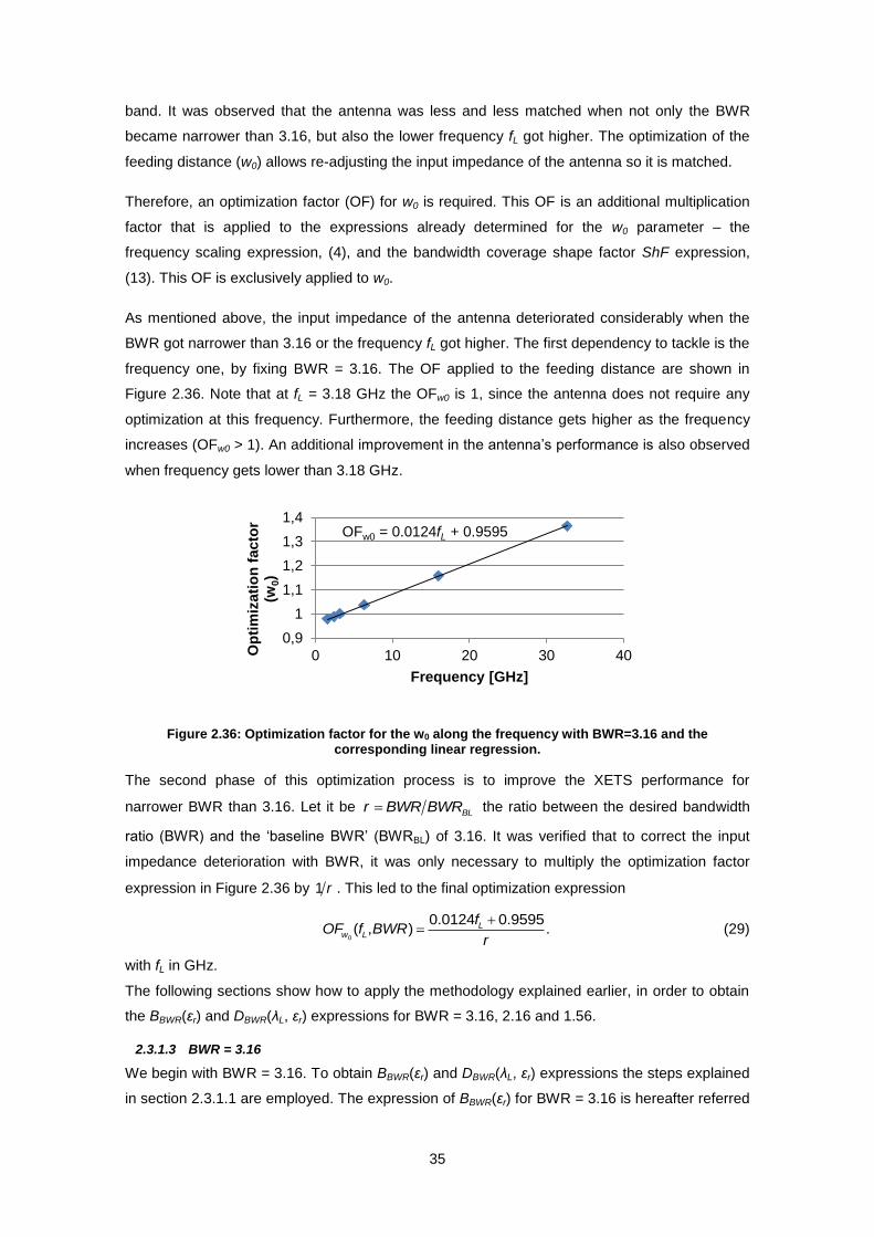
35
band. It was observed that the antenna was less and less matched when not only the BWR
became narrower than 3.16, but also the lower frequency fL got higher. The optimization of the
feeding distance (w0) allows re-adjusting the input impedance of the antenna so it is matched.
Therefore, an optimization factor (OF) for w0 is required. This OF is an additional multiplication
factor that is applied to the expressions already determined for the w0 parameter – the
frequency scaling expression, (4), and the bandwidth coverage shape factor ShF expression,
(13). This OF is exclusively applied to w0.
As mentioned above, the input impedance of the antenna deteriorated considerably when the
BWR got narrower than 3.16 or the frequency fL got higher. The first dependency to tackle is the
frequency one, by fixing BWR = 3.16. The OF applied to the feeding distance are shown in
Figure 2.36. Note that at fL = 3.18 GHz the OFw0 is 1, since the antenna does not require any
optimization at this frequency. Furthermore, the feeding distance gets higher as the frequency
increases (OFw0 > 1). An additional improvement in the antenna’s performance is also observed
when frequency gets lower than 3.18 GHz.
Figure 2.36: Optimization factor for the w0 along the frequency with BWR=3.16 and the corresponding linear regression.
The second phase of this optimization process is to improve the XETS performance for
narrower BWR than 3.16. Let it be BLr BWR BWR the ratio between the desired bandwidth
ratio (BWR) and the ‘baseline BWR’ (BWRBL) of 3.16. It was verified that to correct the input
impedance deterioration with BWR, it was only necessary to multiply the optimization factor
expression in Figure 2.36 by 1 r . This led to the final optimization expression
0
0.0124 0.95( )
95.,L
Lw fOF
rB
fWR
(29)
with fL in GHz.
The following sections show how to apply the methodology explained earlier, in order to obtain
the BBWR(εr) and DBWR(λL, εr) expressions for BWR = 3.16, 2.16 and 1.56.
2.3.1.3 BWR = 3.16
We begin with BWR = 3.16. To obtain BBWR(εr) and DBWR(λL, εr) expressions the steps explained
in section 2.3.1.1 are employed. The expression of BBWR(εr) for BWR = 3.16 is hereafter referred
OFw0 = 0.0124fL + 0.9595
0,9
1
1,1
1,2
1,3
1,4
0 10 20 30 40Op
tim
izati
on
facto
r (w
0)
Frequency [GHz]
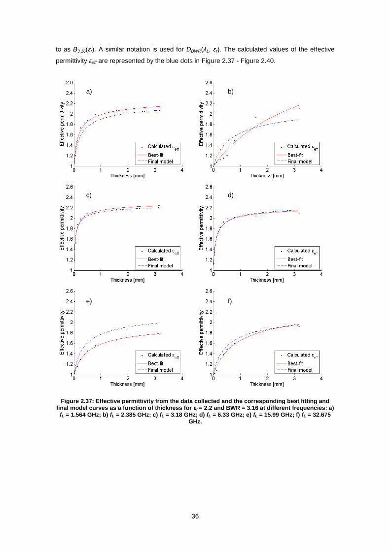
36
to as B3.16(εr). A similar notation is used for DBWR(λL, εr). The calculated values of the effective
permittivity εeff are represented by the blue dots in Figure 2.37 - Figure 2.40.
Figure 2.37: Effective permittivity from the data collected and the corresponding best fitting and final model curves as a function of thickness for εr = 2.2 and BWR = 3.16 at different frequencies: a)
fL = 1.564 GHz; b) fL = 2.385 GHz; c) fL = 3.18 GHz; d) fL = 6.33 GHz; e) fL = 15.99 GHz; f) fL = 32.675 GHz.
a) b)
c) d)
e) f)

37
Figure 2.38: Effective permittivity from the data collected and the corresponding best fitting and final model curves as a function of thickness for εr = 2.33 and BWR = 3.16 at different frequencies:
a) fL = 1.564 GHz; b) fL = 2.385 GHz; c) fL = 3.18 GHz; d) fL = 6.33 GHz; e) fL = 15.99 GHz; f) fL = 32.675 GHz.
a) b)
c) d)
e) f)
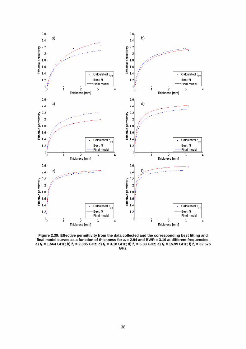
38
Figure 2.39: Effective permittivity from the data collected and the corresponding best fitting and final model curves as a function of thickness for εr = 2.94 and BWR = 3.16 at different frequencies:
a) fL = 1.564 GHz; b) fL = 2.385 GHz; c) fL = 3.18 GHz; d) fL = 6.33 GHz; e) fL = 15.99 GHz; f) fL = 32.675 GHz.
a) b)
c) d)
e) f)
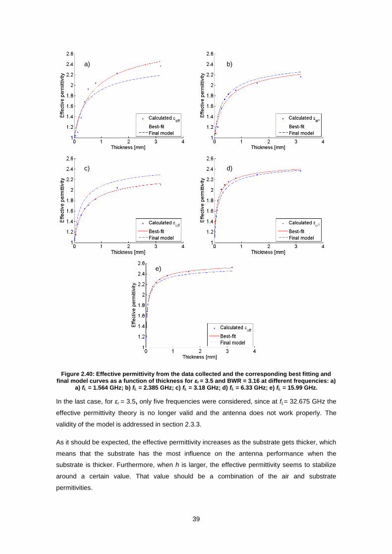
39
Figure 2.40: Effective permittivity from the data collected and the corresponding best fitting and final model curves as a function of thickness for εr = 3.5 and BWR = 3.16 at different frequencies: a)
a) fL = 1.564 GHz; b) fL = 2.385 GHz; c) fL = 3.18 GHz; d) fL = 6.33 GHz; e) fL = 15.99 GHz.
In the last case, for εr = 3.5, only five frequencies were considered, since at fL= 32.675 GHz the
effective permittivity theory is no longer valid and the antenna does not work properly. The
validity of the model is addressed in section 2.3.3.
As it should be expected, the effective permittivity increases as the substrate gets thicker, which
means that the substrate has the most influence on the antenna performance when the
substrate is thicker. Furthermore, when h is larger, the effective permittivity seems to stabilize
around a certain value. That value should be a combination of the air and substrate
permitivities.
a) b)
c) d)
e)
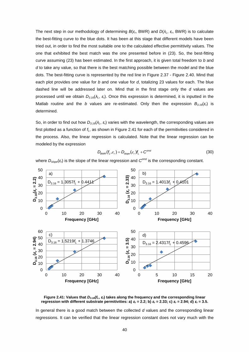
40
The next step in our methodology of determining B(εr, BWR) and D(λL, εr, BWR) is to calculate
the best-fitting curve to the blue dots. It has been at this stage that different models have been
tried out, in order to find the most suitable one to the calculated effective permittivity values. The
one that exhibited the best match was the one presented before in (23). So, the best-fitting
curve assuming (23) has been estimated. In the first approach, it is given total freedom to b and
d to take any value, so that there is the best matching possible between the model and the blue
dots. The best-fitting curve is represented by the red line in Figure 2.37 - Figure 2.40. Mind that
each plot provides one value for b and one value for d, totalizing 23 values for each. The blue
dashed line will be addressed later on. Mind that in the first stage only the d values are
processed until we obtain D3.16(λL, εr). Once this expression is determined, it is inputted in the
Matlab routine and the b values are re-estimated. Only then the expression B3.16(εr) is
determined.
So, in order to find out how D3.16(λL, εr) varies with the wavelength, the corresponding values are
first plotted as a function of fL, as shown in Figure 2.41 for each of the permitivities considered in
the process. Also, the linear regression is calculated. Note that the linear regression can be
modeled by the expression
, )) (( onst
BWR L r slo r LpeD D ff C (30)
where Dslope(εr) is the slope of the linear regression and Const
is the corresponding constant.
Figure 2.41: Values that D3.16(fL, εr) takes along the frequency and the corresponding linear regression with different substrate permitivities: a) εr = 2.2; b) εr = 2.33; c) εr = 2.94; d) εr = 3.5.
In general there is a good match between the collected d values and the corresponding linear
regressions. It can be verified that the linear regression constant does not vary much with the
D3.16 = 1.4013fL + 0.4101
0
10
20
30
40
50
0 10 20 30 40
D3
.16 (ε
r =
2.3
3)
Frequency [GHz]
D3.16 = 1.3057fL + 0.4411
0
10
20
30
40
50
0 10 20 30 40
D3
.16(ε
r =
2.2
)
Frequency [GHz]
D3.16 = 1.5219fL + 1.3746
0
10
20
30
40
50
60
0 10 20 30 40
D3
.16 (ε
r =
2.9
4)
Frequency [GHz]
D3.16 = 2.4317fL + 0.4596
0
10
20
30
40
50
0 5 10 15 20
D3
.16 (ε
r =
3.5
)
Frequency [GHz]
a) b)
c) d)
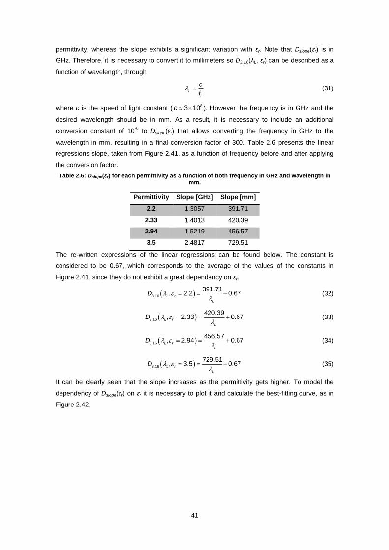
41
permittivity, whereas the slope exhibits a significant variation with εr. Note that Dslope(εr) is in
GHz. Therefore, it is necessary to convert it to millimeters so D3.16(λL, εr) can be described as a
function of wavelength, through
L
L
c
f (31)
where c is the speed of light constant ( 83 10c ). However the frequency is in GHz and the
desired wavelength should be in mm. As a result, it is necessary to include an additional
conversion constant of 10-6
to Dslope(εr) that allows converting the frequency in GHz to the
wavelength in mm, resulting in a final conversion factor of 300. Table 2.6 presents the linear
regressions slope, taken from Figure 2.41, as a function of frequency before and after applying
the conversion factor.
Table 2.6: Dslope(εr) for each permittivity as a function of both frequency in GHz and wavelength in mm.
Permittivity Slope [GHz] Slope [mm]
2.2 1.3057 391.71
2.33 1.4013 420.39
2.94 1.5219 456.57
3.5 2.4817 729.51
The re-written expressions of the linear regressions can be found below. The constant is
considered to be 0.67, which corresponds to the average of the values of the constants in
Figure 2.41, since they do not exhibit a great dependency on εr.
3.16
391.71, 2.2 0.67L r
L
D
(32)
3.16
420.39, 2.33 0.67L r
L
D
(33)
3.16
456.57, 2.94 0.67L r
L
D
(34)
3.16
729.51, 3.5 0.67L r
L
D
(35)
It can be clearly seen that the slope increases as the permittivity gets higher. To model the
dependency of Dslope(εr) on εr it is necessary to plot it and calculate the best-fitting curve, as in
Figure 2.42.

42
Figure 2.42: Slope of D3.16(λL, εr) as a function of the substrate permittivity and the corresponding quadratic expression.
The determination of Dslope(εr) terminates the estimation of the expression of D3.16(λL, εr), which
is summarized below.
2
3.16
321.36 1577 2324.82, 0.67.r r
L r
L
D
(36)
As mentioned before, the values of b are re-calculated by estimating the best-fit to the curves in
Figure 2.37 - Figure 2.40, but this time including (36). This is intended to improve the method’s
accuracy.
After calculating the b values, it has been verified that B3.16(εr) is fairly constant along the
frequency, within a certain permittivity εr. In other words, B3.16(εr) should be a function of εr. So,
the strategy is to calculate the average of the b values for each εr, which leads to the values
shown in Table 2.7.
Table 2.7: Average of the b values for each permittivity.
Permittivity b values (average)
2.2 0.5873
2.33 0.6076
2.94 0.5365
3.5 0.458
Similarly to what has been done to calculate the expression for Dslope(εr), the average of the b
values is plotted as a function of the substrate permittivity, as illustrated in Figure 2.43.
Dslope = 321.36εr2 - 1577.07εr + 2324.82
0
200
400
600
800
2 2,5 3 3,5 4
Slo
pe [
mm
]
Permittivity, εr

43
Figure 2.43: B3.16(εr) as a function of the substrate permittivity and the corresponding quadratic expression.
By estimating the best-fitting curve, we get the following expression for B3.16(εr)
2
3.16 0.0589 0.2266 0.3846.r r rB (37)
In Figure 2.37 - Figure 2.40 it is plotted a dashed blue line. This line represents the effective
permittivity calculated with the XETS effective permittivity final expression. It is possible to see
that there is a reasonable agreement between the red and the blue lines, meaning that the
model represents the XETS quite realistically.
The expressions determined in this sub-section allow designing the XETS with any substrate of
any reasonable thickness with a bandwidth ratio of approximately 3:1.
2.3.1.4 BWR = 2.16
In this section, the BWR is set to 2.16. The effective permittivity is calculated through the
collected ScF. The graphs of the effective permittivity along the thickness are shown in Annex
A.1. The process to determine the expressions for B2.16(εr) and D2.16(λL, εr) is very similar to the
one followed for BWR = 3.16.
The d values obtained for each permittivity are illustrated in Figure 2.44, along with the
corresponding a linear regression of the form 2.16( , ) ( ) onst
L r slope r LD f D f C .
B3.16 = -0.0589εr2 + 0.2266εr + 0.3846
0
0,1
0,2
0,3
0,4
0,5
0,6
0,7
2 2,5 3 3,5 4
B3
.16(ε
r)
Permittivity, εr
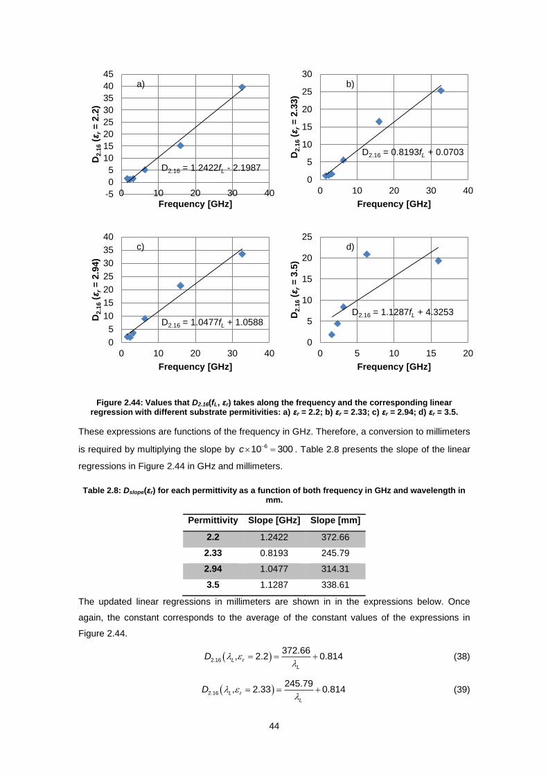
44
Figure 2.44: Values that D2.16(fL, εr) takes along the frequency and the corresponding linear regression with different substrate permitivities: a) εr = 2.2; b) εr = 2.33; c) εr = 2.94; d) εr = 3.5.
These expressions are functions of the frequency in GHz. Therefore, a conversion to millimeters
is required by multiplying the slope by 610 300c . Table 2.8 presents the slope of the linear
regressions in Figure 2.44 in GHz and millimeters.
Table 2.8: Dslope(εr) for each permittivity as a function of both frequency in GHz and wavelength in mm.
Permittivity Slope [GHz] Slope [mm]
2.2 1.2422 372.66
2.33 0.8193 245.79
2.94 1.0477 314.31
3.5 1.1287 338.61
The updated linear regressions in millimeters are shown in in the expressions below. Once
again, the constant corresponds to the average of the constant values of the expressions in
Figure 2.44.
2.16
372.66, 2.2 0.814L r
L
D
(38)
2.16
245.79, 2.33 0.814L r
L
D
(39)
D2.16 = 1.2422fL - 2.1987
-5
0
5
10
15
20
25
30
35
40
45
0 10 20 30 40
D2
.16 (ε
r =
2.2
)
Frequency [GHz]
D2.16 = 0.8193fL + 0.0703
0
5
10
15
20
25
30
0 10 20 30 40
D2
.16 (ε
r =
2.3
3)
Frequency [GHz]
D2.16 = 1.0477fL + 1.0588
0
5
10
15
20
25
30
35
40
0 10 20 30 40
D2
.16 (ε
r =
2.9
4)
Frequency [GHz]
D2.16 = 1.1287fL + 4.3253
0
5
10
15
20
25
0 5 10 15 20
D2
.16 (ε
r =
3.5
)
Frequency [GHz]
a) b)
c) d)
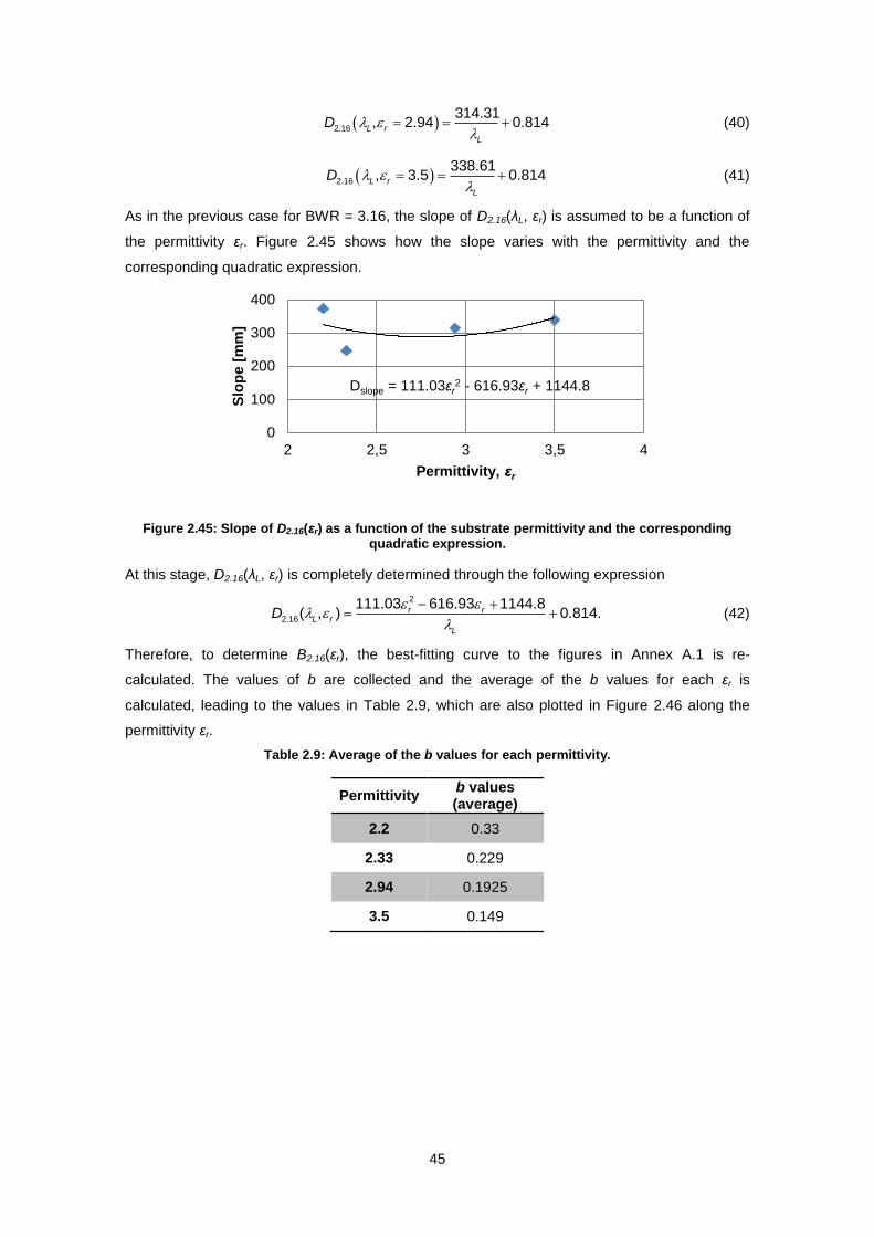
45
2.16
314.31, 2.94 0.814L r
L
D
(40)
2.16
338.61, 3.5 0.814L r
L
D
(41)
As in the previous case for BWR = 3.16, the slope of D2.16(λL, εr) is assumed to be a function of
the permittivity εr. Figure 2.45 shows how the slope varies with the permittivity and the
corresponding quadratic expression.
Figure 2.45: Slope of D2.16(εr) as a function of the substrate permittivity and the corresponding quadratic expression.
At this stage, D2.16(λL, εr) is completely determined through the following expression
2
2.16
111.03 616.93 1144.8( , ) 0.814.r r
L r
L
D
(42)
Therefore, to determine B2.16(εr), the best-fitting curve to the figures in Annex A.1 is re-
calculated. The values of b are collected and the average of the b values for each εr is
calculated, leading to the values in Table 2.9, which are also plotted in Figure 2.46 along the
permittivity εr.
Table 2.9: Average of the b values for each permittivity.
Permittivity b values (average)
2.2 0.33
2.33 0.229
2.94 0.1925
3.5 0.149
Dslope = 111.03εr2 - 616.93εr + 1144.8
0
100
200
300
400
2 2,5 3 3,5 4
Slo
pe [
mm
]
Permittivity, εr
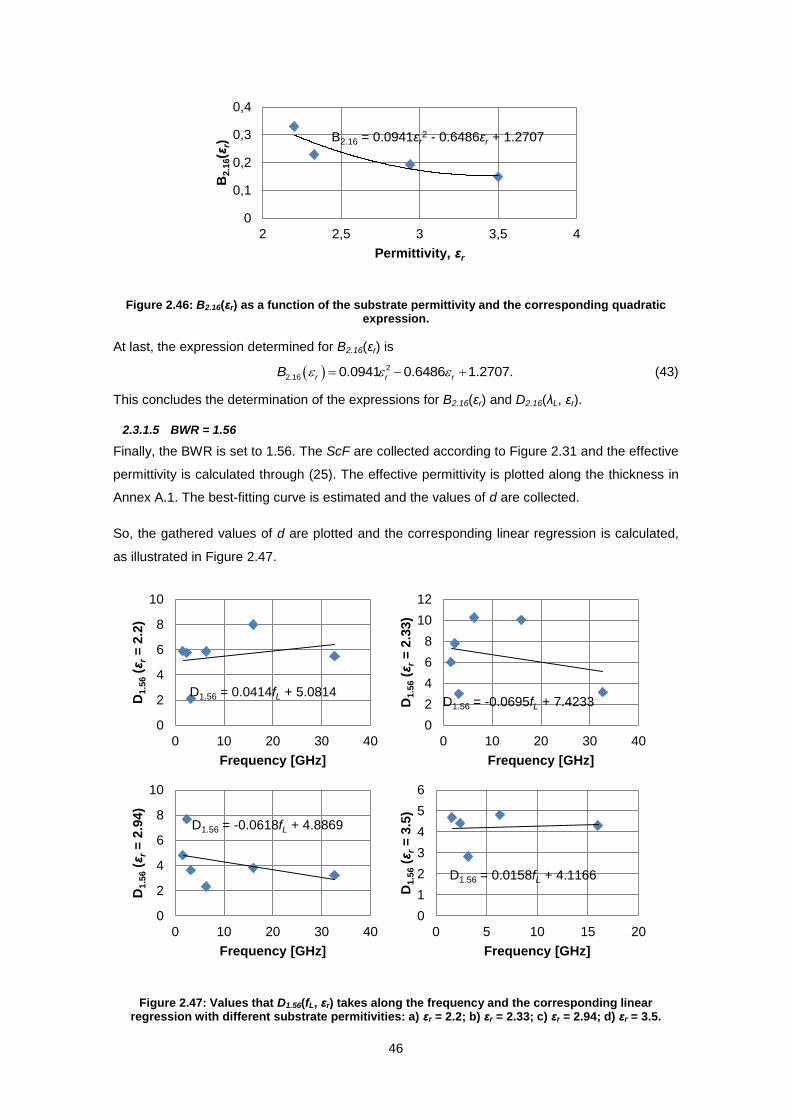
46
Figure 2.46: B2.16(εr) as a function of the substrate permittivity and the corresponding quadratic expression.
At last, the expression determined for B2.16(εr) is
2
2.16 0.0941 0.6486 1.2707.r r rB (43)
This concludes the determination of the expressions for B2.16(εr) and D2.16(λL, εr).
2.3.1.5 BWR = 1.56
Finally, the BWR is set to 1.56. The ScF are collected according to Figure 2.31 and the effective
permittivity is calculated through (25). The effective permittivity is plotted along the thickness in
Annex A.1. The best-fitting curve is estimated and the values of d are collected.
So, the gathered values of d are plotted and the corresponding linear regression is calculated,
as illustrated in Figure 2.47.
Figure 2.47: Values that D1.56(fL, εr) takes along the frequency and the corresponding linear regression with different substrate permitivities: a) εr = 2.2; b) εr = 2.33; c) εr = 2.94; d) εr = 3.5.
B2.16 = 0.0941εr2 - 0.6486εr + 1.2707
0
0,1
0,2
0,3
0,4
2 2,5 3 3,5 4B
2.1
6(ε
r)
Permittivity, εr
D1.56 = 0.0414fL + 5.0814
0
2
4
6
8
10
0 10 20 30 40
D1
.56 (ε
r =
2.2
)
Frequency [GHz]
D1.56 = -0.0695fL + 7.4233
0
2
4
6
8
10
12
0 10 20 30 40
D1
.56 (ε
r =
2.3
3)
Frequency [GHz]
D1.56 = -0.0618fL + 4.8869
0
2
4
6
8
10
0 10 20 30 40
D1
.56 (ε
r =
2.9
4)
Frequency [GHz]
D1.56 = 0.0158fL + 4.1166
0
1
2
3
4
5
6
0 5 10 15 20
D1
.56 (ε
r =
3.5
)
Frequency [GHz]
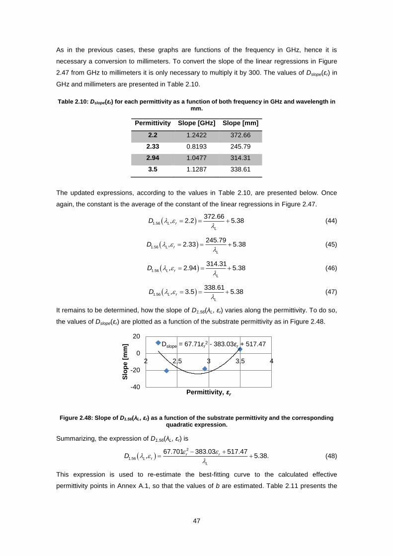
47
As in the previous cases, these graphs are functions of the frequency in GHz, hence it is
necessary a conversion to millimeters. To convert the slope of the linear regressions in Figure
2.47 from GHz to millimeters it is only necessary to multiply it by 300. The values of Dslope(εr) in
GHz and millimeters are presented in Table 2.10.
Table 2.10: Dslope(εr) for each permittivity as a function of both frequency in GHz and wavelength in mm.
Permittivity Slope [GHz] Slope [mm]
2.2 1.2422 372.66
2.33 0.8193 245.79
2.94 1.0477 314.31
3.5 1.1287 338.61
The updated expressions, according to the values in Table 2.10, are presented below. Once
again, the constant is the average of the constant of the linear regressions in Figure 2.47.
1.56
372.66, 2.2 5.38L r
L
D
(44)
1.56
245.79, 2.33 5.38L r
L
D
(45)
1.56
314.31, 2.94 5.38L r
L
D
(46)
1.56
338.61, 3.5 5.38L r
L
D
(47)
It remains to be determined, how the slope of D1.56(λL, εr) varies along the permittivity. To do so,
the values of Dslope(εr) are plotted as a function of the substrate permittivity as in Figure 2.48.
Figure 2.48: Slope of D1.56(λL, εr) as a function of the substrate permittivity and the corresponding quadratic expression.
Summarizing, the expression of D1.56(λL, εr) is
2
1.56
67.701 383.03 517.47, 5.38.r r
L r
L
D
(48)
This expression is used to re-estimate the best-fitting curve to the calculated effective
permittivity points in Annex A.1, so that the values of b are estimated. Table 2.11 presents the
Dslope = 67.71εr2 - 383.03εr + 517.47
-40
-20
0
20
2 2,5 3 3,5 4
Slo
pe [
mm
]
Permittivity, εr
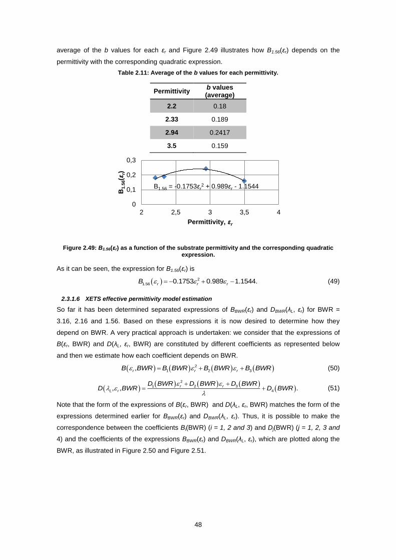
48
average of the b values for each εr and Figure 2.49 illustrates how B1.56(εr) depends on the
permittivity with the corresponding quadratic expression.
Table 2.11: Average of the b values for each permittivity.
Permittivity b values (average)
2.2 0.18
2.33 0.189
2.94 0.2417
3.5 0.159
Figure 2.49: B1.56(εr) as a function of the substrate permittivity and the corresponding quadratic expression.
As it can be seen, the expression for B1.56(εr) is
2
1.56 0.1753 0.989 1.1544.r r rB (49)
2.3.1.6 XETS effective permittivity model estimation
So far it has been determined separated expressions of BBWR(εr) and DBWR(λL, εr) for BWR =
3.16, 2.16 and 1.56. Based on these expressions it is now desired to determine how they
depend on BWR. A very practical approach is undertaken: we consider that the expressions of
B(εr, BWR) and D(λL, εr, BWR) are constituted by different coefficients as represented below
and then we estimate how each coefficient depends on BWR.
2
1 2 3,r r rB BWR B BWR B BWR B BWR (50)
2
1 2 3
4, , .r r
L r
D BWR D BWR D BWRD BWR D BWR
(51)
Note that the form of the expressions of B(εr, BWR) and D(λL, εr, BWR) matches the form of the
expressions determined earlier for BBWR(εr) and DBWR(λL, εr). Thus, it is possible to make the
correspondence between the coefficients Bi(BWR) (i = 1, 2 and 3) and Dj(BWR) (j = 1, 2, 3 and
4) and the coefficients of the expressions BBWR(εr) and DBWR(λL, εr), which are plotted along the
BWR, as illustrated in Figure 2.50 and Figure 2.51.
B1.56 = -0.1753εr2 + 0.989εr - 1.1544
0
0,1
0,2
0,3
2 2,5 3 3,5 4
B1
.56(ε
r)
Permittivity, εr
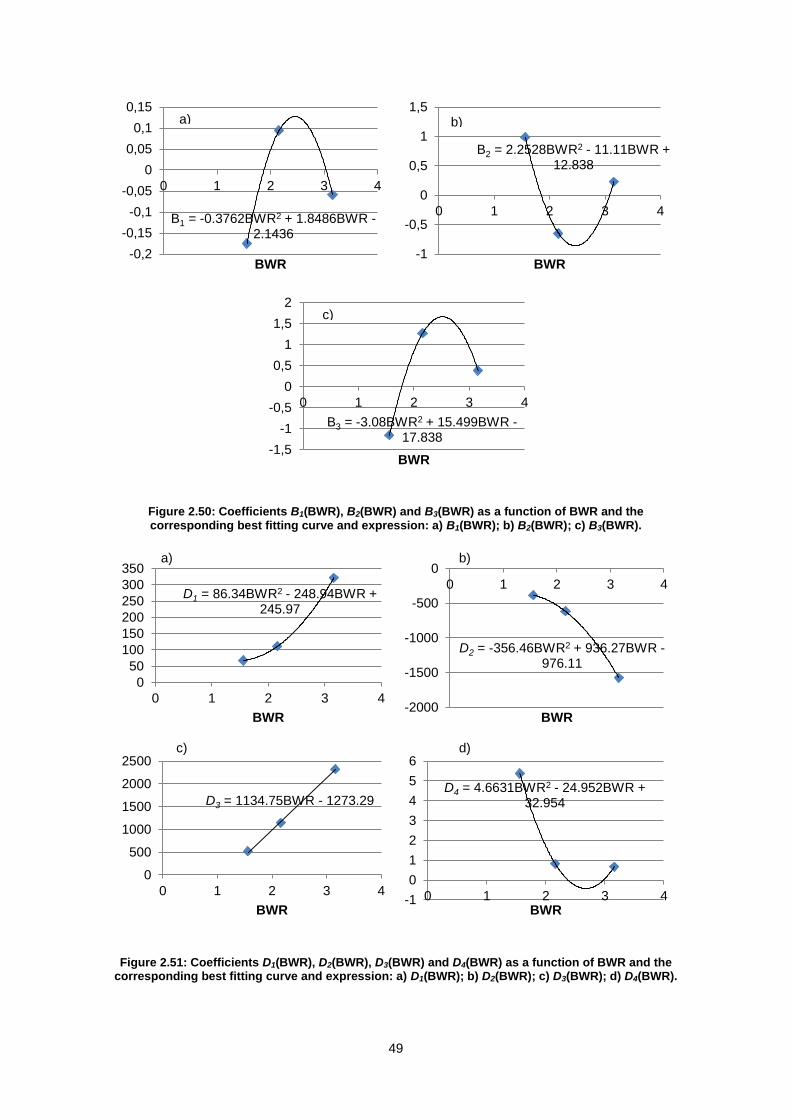
49
Figure 2.50: Coefficients B1(BWR), B2(BWR) and B3(BWR) as a function of BWR and the corresponding best fitting curve and expression: a) B1(BWR); b) B2(BWR); c) B3(BWR).
Figure 2.51: Coefficients D1(BWR), D2(BWR), D3(BWR) and D4(BWR) as a function of BWR and the corresponding best fitting curve and expression: a) D1(BWR); b) D2(BWR); c) D3(BWR); d) D4(BWR).
B1 = -0.3762BWR2 + 1.8486BWR - 2.1436
-0,2
-0,15
-0,1
-0,05
0
0,05
0,1
0,15
0 1 2 3 4
BWR
B2 = 2.2528BWR2 - 11.11BWR + 12.838
-1
-0,5
0
0,5
1
1,5
0 1 2 3 4
BWR
B3 = -3.08BWR2 + 15.499BWR - 17.838
-1,5
-1
-0,5
0
0,5
1
1,5
2
0 1 2 3 4
BWR
a) b)
c)
D4 = 4.6631BWR2 - 24.952BWR + 32.954
-1
0
1
2
3
4
5
6
0 1 2 3 4BWR
D1 = 86.34BWR2 - 248.94BWR + 245.97
0
50
100
150
200
250
300
350
0 1 2 3 4
BWR
D2 = -356.46BWR2 + 936.27BWR - 976.11
-2000
-1500
-1000
-500
0
0 1 2 3 4
BWR
D3 = 1134.75BWR - 1273.29
0
500
1000
1500
2000
2500
0 1 2 3 4
BWR
a) b)
c) d)
50
The match between the points and the best-fitting curves is quite good for all cases. The
expressions for each coefficient are the following.
2
1 0.3762 1.8486 2.14( ) 36B BWR BWRBWR (52)
2
2 2.2528 11.11 12 8( ) . 38B BWR B RBW WR (53)
2
3 3.08 15.499 17.83( ) 8B BWR BWRBWR (54)
2
1 86.34 248.94 245.97( )D BWR BWRBWR (55)
2
2 356.46 936.27 976.( ) 11D BWR BWRBWR (56)
3 1134.7( 5 127) 3.29D BWR RBW (57)
2
4 4.6631 24.952 32.954( )D BWR BWRBWR (58)
At this point the XETS effective permittivity model is complete. Nevertheless, an additional
optimization is required in order to improve the XETS design accuracy.
2.3.2. Final optimization
It should be possible to fully design the antenna, by now. However, a series of test have been
performed, which show that the design of the antenna can be slightly inaccurate in some cases.
As a result, a final optimization is required in order to improve the XETS performance. This time,
the optimization concentrates on the diameter (Dfront), slots length (L), star size (LS) and a scale
factor that is equally applied to all parameters. These parameters allow re-adjusting the input
impedance, so that the real and imaginary parts of the input impedance are approximately 50 Ω
and 0 Ω, respectively. These impedance values correspond to the theoretical values that match
the input impedance. The objective is to improve the reflection coefficient of the antenna along
frequency and BWR by introducing an additional multiplication factor to the respective
parameter expressions.
This optimization is somewhat complex. Therefore, three test cases are considered:
- Case 1: fL = 18 GHz and BWR = 2.23;
- Case 2: fL = 60 GHz and BWR = 1.5;
- Case 3: fL = 18 GHz and BWR = 1.5.
Case 3 represents the ‘bridge’ between the Cases 1 and 2, since it shares the lower frequency
fL with Case 1 and the BWR with Case 2. As a consequence, it allows understanding how each
variable should be optimized: if the multiplication factor of a certain parameter is the same in
Case 1 and Case 3, but it is different in Case 2, then that factor should be a function of the
frequency; otherwise, if the multiplication factor is equal in Cases 2 and 3, but it is different in
Case 1, then it should be a function of BWR. In the three cases it is used a substrate of
thickness 0.254 mm and permittivity εr = 2.2.
The optimization factor expressions are reached by multiplying each parameter (Dfront, L, LS or
the scale factor) individually by a factor until the final values are consistent by trial and error.

51
The final curves and expressions are presented in Figure 2.52. Note that for BWR = 3.16 the
factor should always be 1 (it corresponds to the original case).
Figure 2.52: Optimization factor for each parameter: a) diameter (Dfront); b) Slots length (L); c) Star size (LS); d) scale factor.
It is possible to see that all the parameters share a dependency with the BWR. Also, there is a
good agreement between the best-fit and the points obtained through simulation, resulting in the
expressions:
0.1026 0.6743( )frontDOF RB BWWR (59)
0.0722 0. 6( 7) 7 2LOF BW WRB R (60)
0.0451 5 1) 8( 0.8SLOF BR WRBW (61)
20.2269 1.1477 0.( 1) 36 .ScaleFactorOF BWB BWRW RR (62)
This optimization completes the study of the XETS antenna.
2.3.3. Model analysis and validity
In summary, any user that wants to design the XETS antenna should follow the next steps:
1. Define εr, h, fL and BWR;
2. Calculate the dimensions of the eight XETS parameters without substrate through (4) -
(11) and (13) - (20);
3. Calculate B(εr, BWR) and D(λL, εr, BWR) through (52) - (58);
4. Input the previous values of B(εr, BWR) and D(λL, εr, BWR) in expression (23);
5. Once the effective permittivity is determined, scale the XETS;
6. Multiply the corresponding parameters by the optimization factor (29) and (59) - (62).
OFDfront = 0.1026BWR + 0.6743
0
0,2
0,4
0,6
0,8
1
1,2
0 1 2 3 4
BWR
OFL = 0.0722BWR + 0.7726
0,85
0,9
0,95
1
1,05
0 1 2 3 4
BWR
OFLs = 0.0451BWR + 0.8581
0,92
0,94
0,96
0,98
1
1,02
0 1 2 3 4
BWR
OFScaleFactor = -0.2269BWR2 + 1.1477BWR - 0.361
0
0,2
0,4
0,6
0,8
1
1,2
0 1 2 3 4
BWR
a) b)
c) d)

52
These steps have already been schematized in section 2.1 (Figure 2.2), when the methodology
was explained. By the end of it, the XETS design is complete.
We are now in conditions to design the XETS to work at any frequency, cover any bandwidth
ratio with any substrate of reasonable thickness. However, it is necessary to discuss the validity
of the expressions determined so far. But first, a brief analysis of the model is performed in
order to better understand it.
When the model was defined in (23), it has been explained that the model fulfilled two physical
properties. On the one hand, for a self-sustained antenna, i.e. without substrate, the effective
permittivity should be 1, which corresponds to the air permittivity; on the other hand, when the
substrate thickness is infinitely thick the effective permittivity should become a combination of
the air permittivity with the substrate permittivity. These scenarios are represented in Figure
2.53 a), in which it is shown how the effective permittivity evolves for different values of
substrate permittivity along the thickness with fL = 3.18 GHz and BWR = 3.1. Indeed, when the
thickness is larger, the effective permittivity saturates around a certain value, which is most
certainly a combination of the air with the substrate permitivities. The saturation value becomes
higher for larger substrate permitivities, as expected. Figure 2.53 a) also shows that for a zero
thickness substrate the effective permittivity is 1.
These conclusions can be extended when the substrate thickness becomes electrically large,
i.e. the thickness is large when compared to the wavelength. In other words, considering εr
constant, when the frequency increases, the effective permittivity should saturate in a value that
is a combination of both air and substrate permitivities. This is confirmed by Figure 2.53 b), in
which is considered a permittivity of εr = 2.2 and BWR = 3.1.
Finally, a third scenario can be taken into consideration, as in Figure 2.53 c). This time, the
frequency and substrate permittivity are set to 3.18 GHz and 2.2, respectively, and the BWR is
swept. It is possible to see that the effective permittivity takes higher values as the bandwidth
ratio increases. At lower BWR the effective permittivity rapidly saturates.

53
Figure 2.53: Effective permittivity along the thickness: a) Substrate permittivity εr sweep with BWR = 3.1 and fL = 3.18 GHz; b) Lower frequency fL sweep with BWR = 3.1 and εr = 2.2; c) BWR sweep
with fL = 3.18 GHz and εr = 2.2.
This brief analysis makes it easier to discuss the validity of the model. According to the
microstrip theory, the effective permittivity model for a microstrip line is valid when the width of
the microstrip, Wms, is wider than the height of the substrate, hms, i.e. 1ms msW h . A similar
expression is verified for the model of the XETS. However, the expression is not so simple. Yet,
it should be expected that when the wavelength is much smaller than the substrate thickness,
the model may become invalid. Therefore, the expression must take into account the ratio h /,
in which h is the substrate thickness and λ is the wavelength.
To calculate the validity condition, a series of full-wave simulations are performed for different
values of h and substrate permittivity. The objective is to determine the maximum frequency up
to which the model is valid. Then, the ratio h / is calculated. The results are plotted as
functions of permittivity and h / as in Figure 2.54.
a) b)
c)

54
Figure 2.54: Validity expression as a function of εr and h .
These results were obtained by adopting a rather conservative approach, in order to guarantee
the correct design of the XETS. In fact, in some situations, in which the substrate permittivity is
lower, the model is still valid and can be extended beyond this validity expression, to higher
frequencies and/or thicknesses.
The validity condition is that h cannot be larger than the expression in Figure 2.54, which
leads to the following validity expression.
20.0169 0.1361 0.2777r r
h
2(0.0169 0.1361 0.2777) 1r rh
(63)
The expression (63) sets the physical limitation of the model. An additional physical limitation is
that the effective permittivity cannot take less than 1 value. The last two limitations can be
represented as follows
1eff (64)
1 0.Dh (65)
In (65), D(λL, εr, BWR) is determined through the (51) and h is the substrate thickness in
millimeters. The expression (64) can be developed until the following expression is obtained
1 1Dh (66)
So, the validity condition is that (65) and (66) are both verified at the same time. Note that (66)
is more restrictive than (65). Therefore, the validity conditions are simply (63) and (66).
2.4. The XETS calculator
The goal of this thesis was to develop an automatic XETS design generator. It has been
accomplished in the previous sections, by following a thorough methodology due to the
complexity of the antenna. However, from the user point of view the design of the antenna is
much simpler. In fact, the user only has to specify a few inputs (desired lower frequency fL,
bandwidth ratio BWR and substrate permittivity εr and thickness h) and the XETS calculator will
return the dimensions of the antenna’s parameter necessary to fully design the XETS. The
XETS calculator interface developed in Matlab is represented in Figure 2.55.
h/λ = 0.0169εr2 - 0.1361εr + 0.2777
0
0,02
0,04
0,06
0,08
0 1 2 3 4 5
Rati
o h
/λ
Permittivity, εr
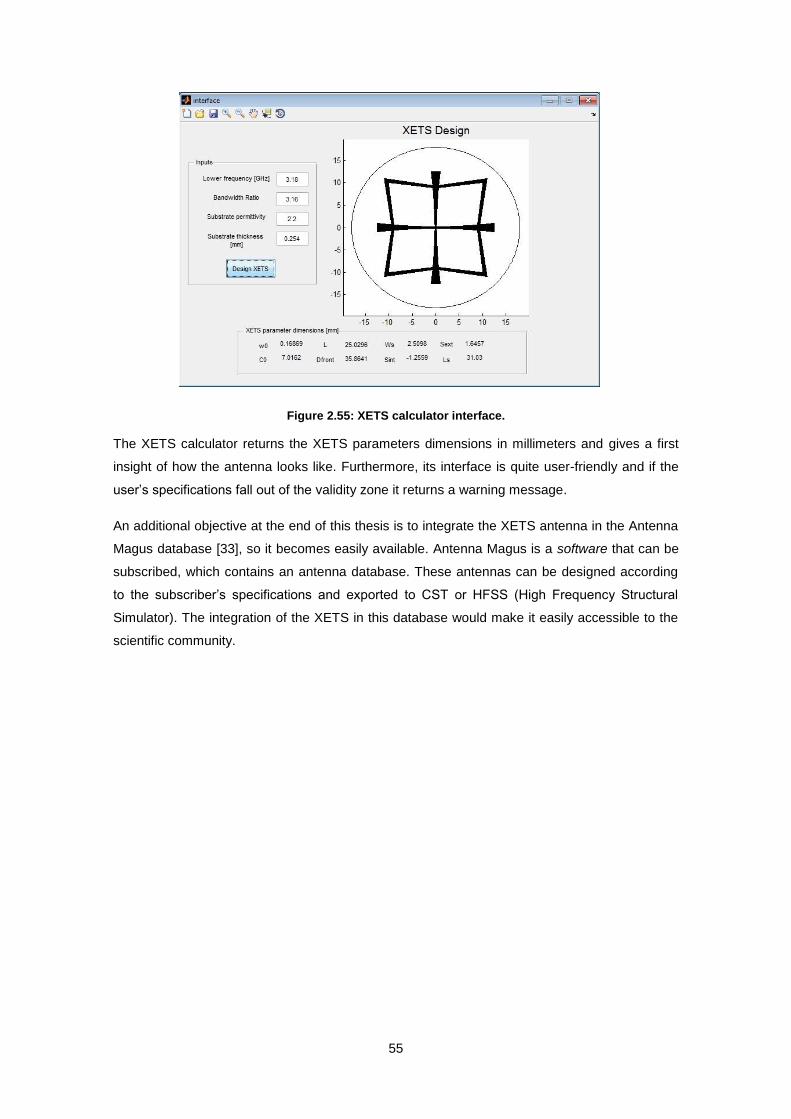
55
Figure 2.55: XETS calculator interface.
The XETS calculator returns the XETS parameters dimensions in millimeters and gives a first
insight of how the antenna looks like. Furthermore, its interface is quite user-friendly and if the
user’s specifications fall out of the validity zone it returns a warning message.
An additional objective at the end of this thesis is to integrate the XETS antenna in the Antenna
Magus database [33], so it becomes easily available. Antenna Magus is a software that can be
subscribed, which contains an antenna database. These antennas can be designed according
to the subscriber’s specifications and exported to CST or HFSS (High Frequency Structural
Simulator). The integration of the XETS in this database would make it easily accessible to the
scientific community.
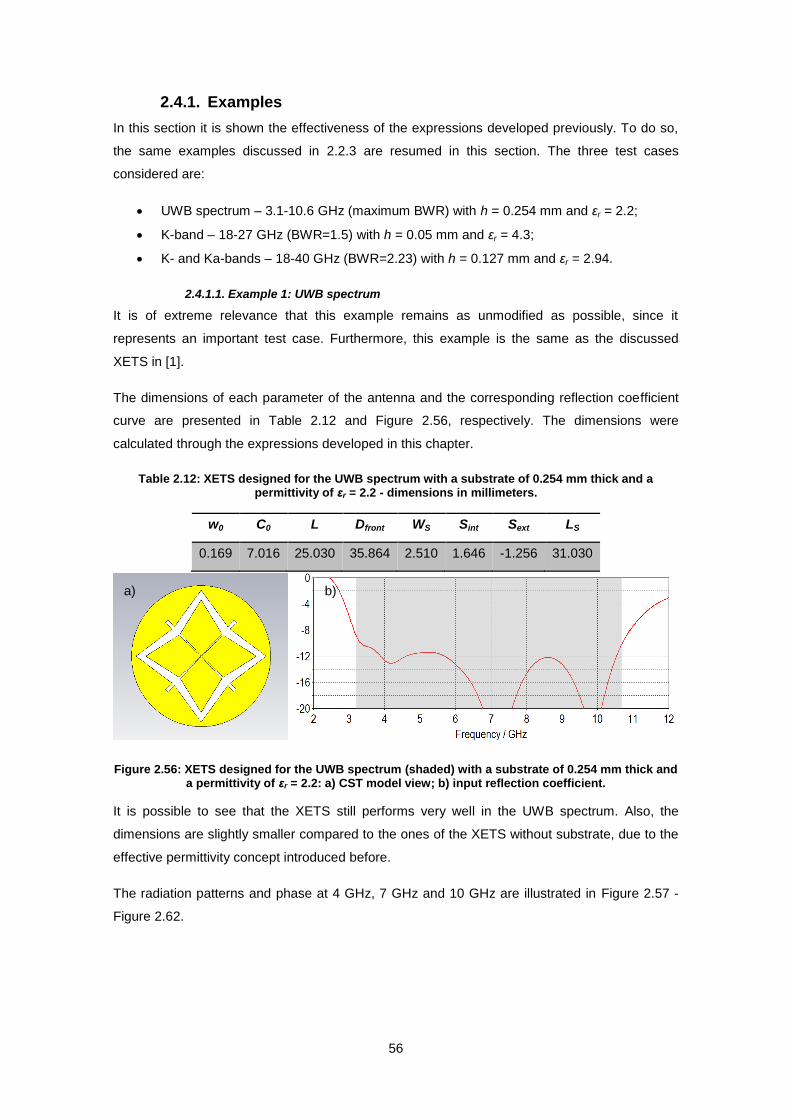
56
2.4.1. Examples
In this section it is shown the effectiveness of the expressions developed previously. To do so,
the same examples discussed in 2.2.3 are resumed in this section. The three test cases
considered are:
UWB spectrum – 3.1-10.6 GHz (maximum BWR) with h = 0.254 mm and εr = 2.2;
K-band – 18-27 GHz (BWR=1.5) with h = 0.05 mm and εr = 4.3;
K- and Ka-bands – 18-40 GHz (BWR=2.23) with h = 0.127 mm and εr = 2.94.
2.4.1.1. Example 1: UWB spectrum
It is of extreme relevance that this example remains as unmodified as possible, since it
represents an important test case. Furthermore, this example is the same as the discussed
XETS in [1].
The dimensions of each parameter of the antenna and the corresponding reflection coefficient
curve are presented in Table 2.12 and Figure 2.56, respectively. The dimensions were
calculated through the expressions developed in this chapter.
Table 2.12: XETS designed for the UWB spectrum with a substrate of 0.254 mm thick and a permittivity of εr = 2.2 - dimensions in millimeters.
w0 C0 L Dfront WS Sint Sext LS
0.169 7.016 25.030 35.864 2.510 1.646 -1.256 31.030
Figure 2.56: XETS designed for the UWB spectrum (shaded) with a substrate of 0.254 mm thick and a permittivity of εr = 2.2: a) CST model view; b) input reflection coefficient.
It is possible to see that the XETS still performs very well in the UWB spectrum. Also, the
dimensions are slightly smaller compared to the ones of the XETS without substrate, due to the
effective permittivity concept introduced before.
The radiation patterns and phase at 4 GHz, 7 GHz and 10 GHz are illustrated in Figure 2.57 -
Figure 2.62.
a) b)

57
Figure 2.57: XETS designed for the UWB spectrum with a substrate of 0.254 mm thick and a permittivity of εr = 2.2 – 3D view of the radiation pattern at 4 GHz.
Figure 2.58: XETS designed for the UWB spectrum with a substrate of 0.254 mm thick and a permittivity of εr = 2.2 - simulated radiation pattern and phase at 4 GHz in the E- (red) and H-planes
(green): a) radiation pattern; b) phase.
Figure 2.59: XETS designed for the UWB spectrum with a substrate of 0.254 mm thick and a permittivity of εr = 2.2 – 3D view of the radiation pattern at 7 GHz.
Figure 2.60: XETS designed for the UWB spectrum with a substrate of 0.254 mm thick and a permittivity of εr = 2.2 - simulated radiation pattern and phase at 7 GHz in the E- (red) and H-planes
(green): a) radiation pattern; b) phase.
a) b)
a) b)
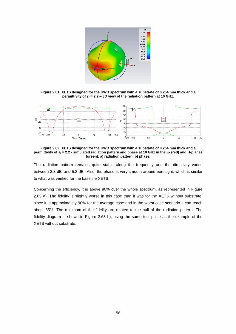
58
Figure 2.61: XETS designed for the UWB spectrum with a substrate of 0.254 mm thick and a permittivity of εr = 2.2 – 3D view of the radiation pattern at 10 GHz.
Figure 2.62: XETS designed for the UWB spectrum with a substrate of 0.254 mm thick and a permittivity of εr = 2.2 - simulated radiation pattern and phase at 10 GHz in the E- (red) and H-planes
(green): a) radiation pattern; b) phase.
The radiation pattern remains quite stable along the frequency and the directivity varies
between 2.8 dBi and 5.3 dBi. Also, the phase is very smooth around boresight, which is similar
to what was verified for the baseline XETS.
Concerning the efficiency, it is above 90% over the whole spectrum, as represented in Figure
2.63 a). The fidelity is slightly worse in this case than it was for the XETS without substrate,
since it is approximately 90% for the average case and in the worst case scenario it can reach
about 85%. The minimum of the fidelity are related to the null of the radiation pattern. The
fidelity diagram is shown in Figure 2.63 b), using the same test pulse as the example of the
XETS without substrate.
a) b)
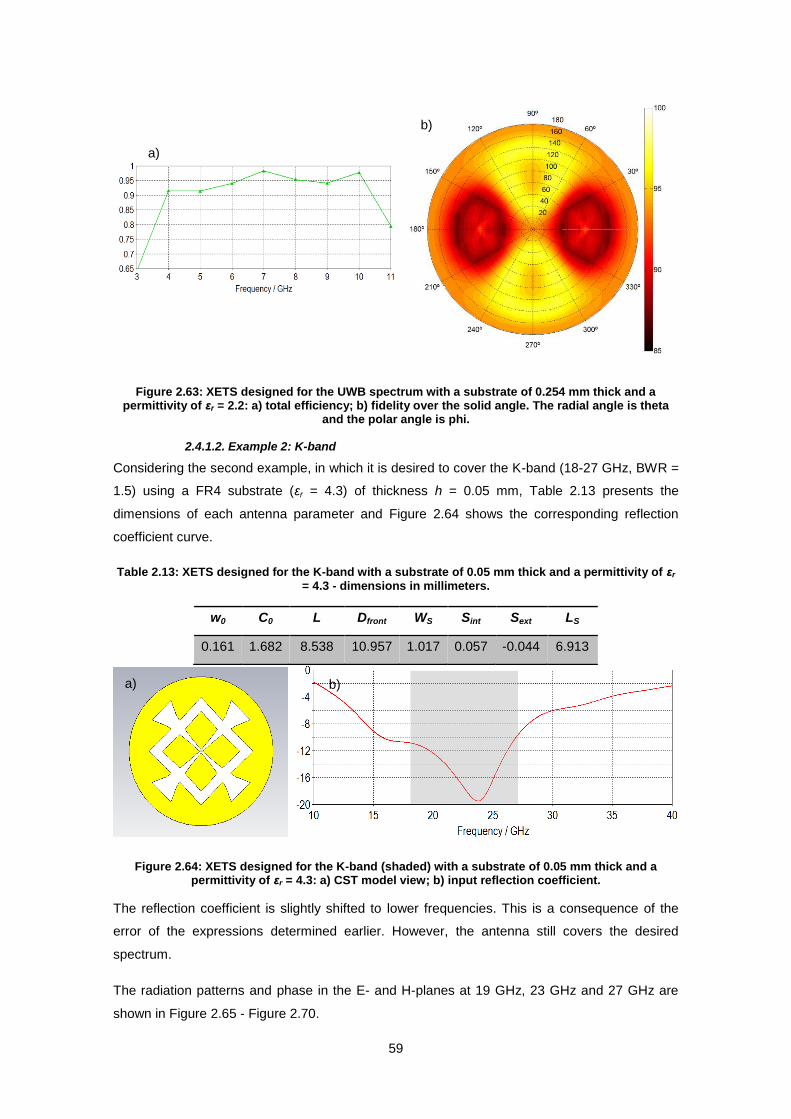
59
Figure 2.63: XETS designed for the UWB spectrum with a substrate of 0.254 mm thick and a permittivity of εr = 2.2: a) total efficiency; b) fidelity over the solid angle. The radial angle is theta
and the polar angle is phi.
2.4.1.2. Example 2: K-band
Considering the second example, in which it is desired to cover the K-band (18-27 GHz, BWR =
1.5) using a FR4 substrate (εr = 4.3) of thickness h = 0.05 mm, Table 2.13 presents the
dimensions of each antenna parameter and Figure 2.64 shows the corresponding reflection
coefficient curve.
Table 2.13: XETS designed for the K-band with a substrate of 0.05 mm thick and a permittivity of εr = 4.3 - dimensions in millimeters.
w0 C0 L Dfront WS Sint Sext LS
0.161 1.682 8.538 10.957 1.017 0.057 -0.044 6.913
Figure 2.64: XETS designed for the K-band (shaded) with a substrate of 0.05 mm thick and a permittivity of εr = 4.3: a) CST model view; b) input reflection coefficient.
The reflection coefficient is slightly shifted to lower frequencies. This is a consequence of the
error of the expressions determined earlier. However, the antenna still covers the desired
spectrum.
The radiation patterns and phase in the E- and H-planes at 19 GHz, 23 GHz and 27 GHz are
shown in Figure 2.65 - Figure 2.70.
a)
b)
a) b)
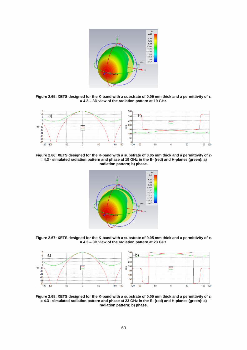
60
Figure 2.65: XETS designed for the K-band with a substrate of 0.05 mm thick and a permittivity of εr = 4.3 – 3D view of the radiation pattern at 19 GHz.
Figure 2.66: XETS designed for the K-band with a substrate of 0.05 mm thick and a permittivity of εr = 4.3 - simulated radiation pattern and phase at 19 GHz in the E- (red) and H-planes (green): a)
radiation pattern; b) phase.
Figure 2.67: XETS designed for the K-band with a substrate of 0.05 mm thick and a permittivity of εr = 4.3 – 3D view of the radiation pattern at 23 GHz.
Figure 2.68: XETS designed for the K-band with a substrate of 0.05 mm thick and a permittivity of εr = 4.3 - simulated radiation pattern and phase at 23 GHz in the E- (red) and H-planes (green): a)
radiation pattern; b) phase.
a) b)
a) b)
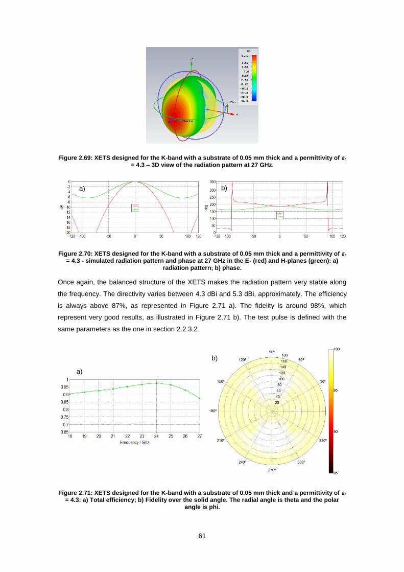
61
Figure 2.69: XETS designed for the K-band with a substrate of 0.05 mm thick and a permittivity of εr = 4.3 – 3D view of the radiation pattern at 27 GHz.
Figure 2.70: XETS designed for the K-band with a substrate of 0.05 mm thick and a permittivity of εr = 4.3 - simulated radiation pattern and phase at 27 GHz in the E- (red) and H-planes (green): a)
radiation pattern; b) phase.
Once again, the balanced structure of the XETS makes the radiation pattern very stable along
the frequency. The directivity varies between 4.3 dBi and 5.3 dBi, approximately. The efficiency
is always above 87%, as represented in Figure 2.71 a). The fidelity is around 98%, which
represent very good results, as illustrated in Figure 2.71 b). The test pulse is defined with the
same parameters as the one in section 2.2.3.2.
Figure 2.71: XETS designed for the K-band with a substrate of 0.05 mm thick and a permittivity of εr = 4.3: a) Total efficiency; b) Fidelity over the solid angle. The radial angle is theta and the polar
angle is phi.
a) b)
a)
b)

62
2.4.1.3. Example 3: K- and Ka-bands
In the final example it is desired to cover the K- and Ka-bands (18-40 GHz – BWR = 2.23) with a
substrate permittivity εr = 2.94 and thickness h = 0.127 mm. The dimensions and the reflection
coefficient are presented in Table 2.14 and Figure 2.72, respectively.
Table 2.14: XETS designed for the K- and Ka-bands with a substrate of 0.127 mm thick and a permittivity of εr = 2.94 - dimensions in millimeters.
w0 C0 L Dfront WS Sint Sext LS
0.075 1.635 6.714 7.665 0.702 0.179 -0.137 6.256
Figure 2.72: XETS designed for the K- and Ka-bands (shaded) with a substrate of 0.127 mm thick and a permittivity of εr = 2.94: a) CST model view; b) input reflection coefficient.
The input reflection coefficient is slightly shifted to lower frequencies and is a bit narrower than
desired. Nevertheless, the expressions still provide a reasonable first approximation.
Furthermore, the upper frequency can be improved by simply re-adjusting the slots length, L, by
multiplying it by a factor.
Concerning the radiation pattern and phase, Figure 2.72 - Figure 2.78 show that the radiation
patterns remain very stable along the frequency and the phase varies very smoothly around
boresight.
Figure 2.73: XETS designed for the K- and Ka-bands with a substrate of 0.127 mm thick and a permittivity of εr = 2.94 – 3D view of the radiation pattern at 20 GHz.
a) b)

63
Figure 2.74: XETS designed for the K- and Ka-bands with a substrate of 0.127 mm thick and a permittivity of εr = 2.94 - simulated radiation pattern and phase at 20 GHz in the E- (red) and H-
planes (green): a) radiation pattern; b) phase.
Figure 2.75: XETS designed for the K- and Ka-bands with a substrate of 0.127 mm thick and a permittivity of εr = 2.94 – 3D view of the radiation pattern at 29 GHz.
Figure 2.76: XETS designed for the K- and Ka-bands with a substrate of 0.127 mm thick and a permittivity of εr = 2.94 - simulated radiation pattern and phase at 29 GHz in the E- (red) and H-
planes (green): a) radiation pattern; b) phase.
Figure 2.77: XETS designed for the K- and Ka-bands with a substrate of 0.127 mm thick and a permittivity of εr = 2.94 – 3D view of the radiation pattern at 39 GHz.
a) b)
a) b)
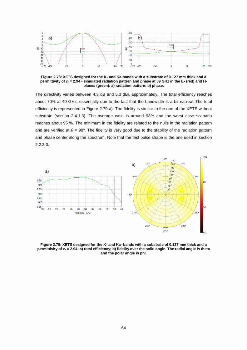
64
Figure 2.78: XETS designed for the K- and Ka-bands with a substrate of 0.127 mm thick and a permittivity of εr = 2.94 - simulated radiation pattern and phase at 39 GHz in the E- (red) and H-
planes (green): a) radiation pattern; b) phase.
The directivity varies between 4.3 dB and 5.3 dBi, approximately. The total efficiency reaches
about 70% at 40 GHz, essentially due to the fact that the bandwidth is a bit narrow. The total
efficiency is represented in Figure 2.79 a). The fidelity is similar to the one of the XETS without
substrate (section 2.4.1.3). The average case is around 98% and the worst case scenario
reaches about 95 %. The minimum in the fidelity are related to the nulls in the radiation pattern
and are verified at θ = 90º. The fidelity is very good due to the stability of the radiation pattern
and phase center along the spectrum. Note that the test pulse shape is the one used in section
2.2.3.3.
Figure 2.79: XETS designed for the K- and Ka- bands with a substrate of 0.127 mm thick and a permittivity of εr = 2.94: a) total efficiency; b) fidelity over the solid angle. The radial angle is theta
and the polar angle is phi.
a) b)
a)
b)
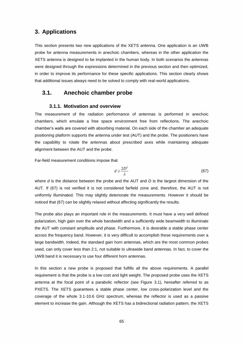
65
3. Applications
This section presents two new applications of the XETS antenna. One application is an UWB
probe for antenna measurements in anechoic chambers, whereas in the other application the
XETS antenna is designed to be implanted in the human body. In both scenarios the antennas
were designed through the expressions determined in the previous section and then optimized,
in order to improve its performance for these specific applications. This section clearly shows
that additional issues always need to be solved to comply with real-world applications.
3.1. Anechoic chamber probe
3.1.1. Motivation and overview
The measurement of the radiation performance of antennas is performed in anechoic
chambers, which emulate a free space environment free from reflections. The anechoic
chamber’s walls are covered with absorbing material. On each side of the chamber an adequate
positioning platform supports the antenna under test (AUT) and the probe. The positioners have
the capability to rotate the antennas about prescribed axes while maintaining adequate
alignment between the AUT and the probe.
Far-field measurement conditions impose that
22D
d
(67)
where d is the distance between the probe and the AUT and D is the largest dimension of the
AUT. If (67) is not verified it is not considered farfield zone and, therefore, the AUT is not
uniformly illuminated. This may slightly deteriorate the measurements. However it should be
noticed that (67) can be slightly relaxed without affecting significantly the results.
The probe also plays an important role in the measurements. It must have a very well defined
polarization, high gain over the whole bandwidth and a sufficiently wide beamwidth to illuminate
the AUT with constant amplitude and phase. Furthermore, it is desirable a stable phase center
across the frequency band. However, it is very difficult to accomplish these requirements over a
large bandwidth. Indeed, the standard gain horn antennas, which are the most common probes
used, can only cover less than 2:1, not suitable to ultrawide band antennas. In fact, to cover the
UWB band it is necessary to use four different horn antennas.
In this section a new probe is proposed that fulfills all the above requirements. A parallel
requirement is that the probe is a low cost and light weight. The proposed probe uses the XETS
antenna at the focal point of a parabolic reflector (see Figure 3.1), hereafter referred to as
PXETS. The XETS guarantees a stable phase center, low cross-polarization level and the
coverage of the whole 3.1-10.6 GHz spectrum, whereas the reflector is used as a passive
element to increase the gain. Although the XETS has a bidirectional radiation pattern, the XETS

66
radiation in the direction opposite to the parabolic reflector does not interfere significantly with
the parabola-originated collimated beam.
3.1.2. Design
To design such a probe, a few aspects must be taken into consideration. The XETS is fed
through an EZ-47 semi-rigid coaxial cable (1.19 mm diameter), which extends from the XETS to
the back of the reflector through its center. The cable is soldered between two opposing petals
of the XETS and includes a U-turn near the antenna to try to keep the symmetry at the possible
extent. This has a positive impact on cross-polarization level. A rigid structure is required to
hold the XETS precisely in place and prevent the thin coaxial cable from bending. A cylindrical
styrofoam piece (with a diameter of 50 mm) is used with this objective, as shown in Figure 3.1
a). It is a self-sustained structure, that does not need struts and so has minimum blocking of the
parabola aperture. The styrofoam’s permittivity is very close to the air’s ( ), as proven in
Annex A.1, so it can be considered to be ‘invisible’ in the band of interest. The total length of the
cable is approximately 145 mm, which corresponds to the focal distance of the reflector. The
parabola’s diameter is D = 350 mm.
Figure 3.1: Probe CST models: a) XETS with the reflector; b) XETS in the styrofoam with the absorber near the antenna – position 1; c) XETS in the styrofoam with the absorber far from the
antenna – position 2 – and detail of the cable’s U-turn.
The XETS is designed to cover the UWB spectrum, through the expressions determined before,
followed by a small optimization. The dimensions are presented in Table 3.1. The
corresponding reflection coefficient is represented by the blue curve in Figure 3.2 b).
Table 3.1: XETS dimensions in millimeters for the UWB probe application.
w0 C0 L Dfront WS Sint Sext LS
0.17 7 25 36 2.5 1.651 -1.251 31
a)
Styrofoam
XETS
b)
c)
Absorber
Absorber
a)

67
Figure 3.2: a) XETS CST model; b) Simulated input reflection coefficient of the XETS for the UWB probe application.
The dashed blue line represents the s11 simulation results for the XETS fed by a discrete port in
free space, whereas the solid blue line corresponds to the XETS fed by the 145 mm cable with
the presence of the reflector. By comparing both situations, it is seen that the very long coaxial
cable together with the reflected wave from the parabola ruins the XETS performance at the
lower frequencies. The stray currents on the outer conductor of the cable contribute to radiation.
In order to improve the |S11|, an absorber is included around the cable to eliminate the electric
field originated by the currents flowing in the external conductor of the cable. The total
dimensions of the absorber are 50 × 18 × 18 mm3.
The absorber is tested in two different positions: near the antenna – position 1 – (Figure 3.1 b))
and far from it – position 2 – (Figure 3.1 c)). The red and green curves in Figure 3.2 represent
the simulated input reflection coefficient when the absorber is in the first and second positions,
respectively. When the absorber is placed in position 2, the input reflection coefficient reaches
about -6 dB near 5 GHz, but it otherwise improves the antenna’s performance, compared to the
situation without absorber. When the absorber is in position 1, the reflection coefficient is slightly
worse exceeding the -10 dB limit until 6.5 GHz. Another issue requires a detailed analysis: it is
the shadow originated by the absorber in the reflector illumination. Simulations show a severe
radiation pattern break-up for high frequencies when the absorber is located in position 1.
These conclusions were verified with a manufactured prototype shown in Figure 3.3. The metal
pieces in Figure 3.3 b) and c) are used for attaching the styrofoam cylinder to the reflector. The
input reflection coefficient of the feed prototype when mounted on the reflector was measured.
The results are illustrated in Figure 3.4, for the absorber in position 1 (a) and in position 2 (b).
a) b)

68
Figure 3.3: Probe prototype: a) XETS with the reflector in the anechoic chamber positioner; b) XETS in the styrofoam with the absorber near the antenna; c) XETS in the styrofoam with the
absorber far from the antenna.
Figure 3.4: Measured and simulated input reflection coefficient: a) Position 1 - absorber near the antenna; b) Position 2 - absorber far from the antenna.
In both cases, the measurements match the simulated results quite well, apart from some ripple
due to possible differences between the measurement set-up and the simulated model. The
measurements show acceptable s11 performance for the absorber in position 1, better than
predicted by simulations. However, the absorber in position 2 creates a smaller “shadow” zone
in the reflector illumination, thus avoiding the significant pattern breakup of position 1.
Nevertheless, the cross-polarization level should be slightly higher. Since the radiation pattern
breakup in position 1 is detrimental of the probe application, the absorber is placed in position 2.
3.1.3. Measurements
The PXETS radiation patterns were measured in the anechoic chamber, as illustrated in Figure
3.5. A total of four different standard gain horn antennas were used as probe, in order to cover
the entire UWB band. Figure 3.6 - Figure 3.8 show the radiation pattern at 4 GHz, 7 GHz and 10
GHz.
b)
c)
Styrofoam Absorber
Absorber Styrofoam
a)
Attaching metal pieces
a) b)
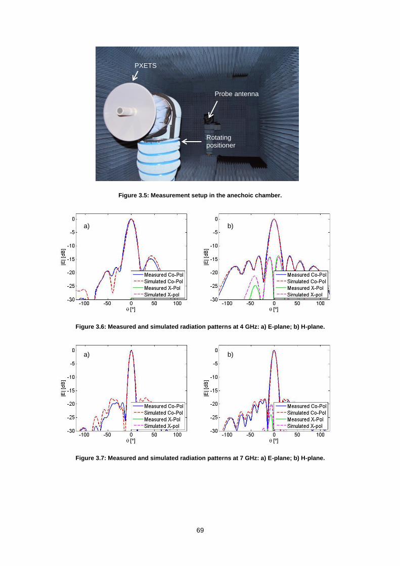
69
Figure 3.5: Measurement setup in the anechoic chamber.
Figure 3.6: Measured and simulated radiation patterns at 4 GHz: a) E-plane; b) H-plane.
Figure 3.7: Measured and simulated radiation patterns at 7 GHz: a) E-plane; b) H-plane.
Probe antenna
PXETS
Rotating positioner
a) b)
a) b)

70
Figure 3.8: Measured and simulated radiation patterns at 10 GHz: a) E-plane; b) H-plane.
The similarity between the measured and the simulated results is very good (despite the fact
that the far-field condition at the IT anechoic chamber for the 350 mm reflector diameter is not
met for f > 5.82 GHz). The radiation pattern in the H-plane is symmetric, since the whole
structure is symmetric in that plane. Also, the cross-polarization level is always below -30 dB at
boresight across the whole spectrum. However, in the H-plane at 10 GHz the measured
radiation pattern exhibits small “shoulders” that may be a consequence of a small misalignment
of the positioners of the anechoic chamber or a consequence of the AUT phase center not
being positioned exactly at the rotating axis of the positioner. Either of these cases, or a
combination of both, may be causing the sidelobes in the radiation pattern to be reasonably
high. Nevertheless regarding the probe application, these “shoulders” are not very problematic.
For the probe application, the beamwidth of interest is typically < 5º near its boresight,
corresponding to the AUT area of illumination. It is noted that the obtained radiation pattern is
very well defined and symmetrical in this interval (although degrading towards 10 GHz). Another
characteristic that may be desirable to know for a probe is its exact gain value at each
frequency. The PXETS gain is determined by the “gain comparison method”. The method relies
on the Friis formula and requires a standard gain horn,
102log
4r
r tBt d
d dB
B
PG G
P d
(68)
Two consecutive measurements of rP tP are performed: the first includes the PXETS (with
unknown gain GAUT) and a probe antenna, whereas the second one uses a standard gain horn
antenna (with gain Gs) and the same probe antenna as before. Combining the result of (68) for
the two measurements we get:
r rP PAUT SAUT S
t t
G GP P
(69)
The measured gain of the PXETS is shown in Figure 3.9. Note that the measurement system
full-port calibration is not ideal at it involves a long cable for the “through” measurement; this
a) b)
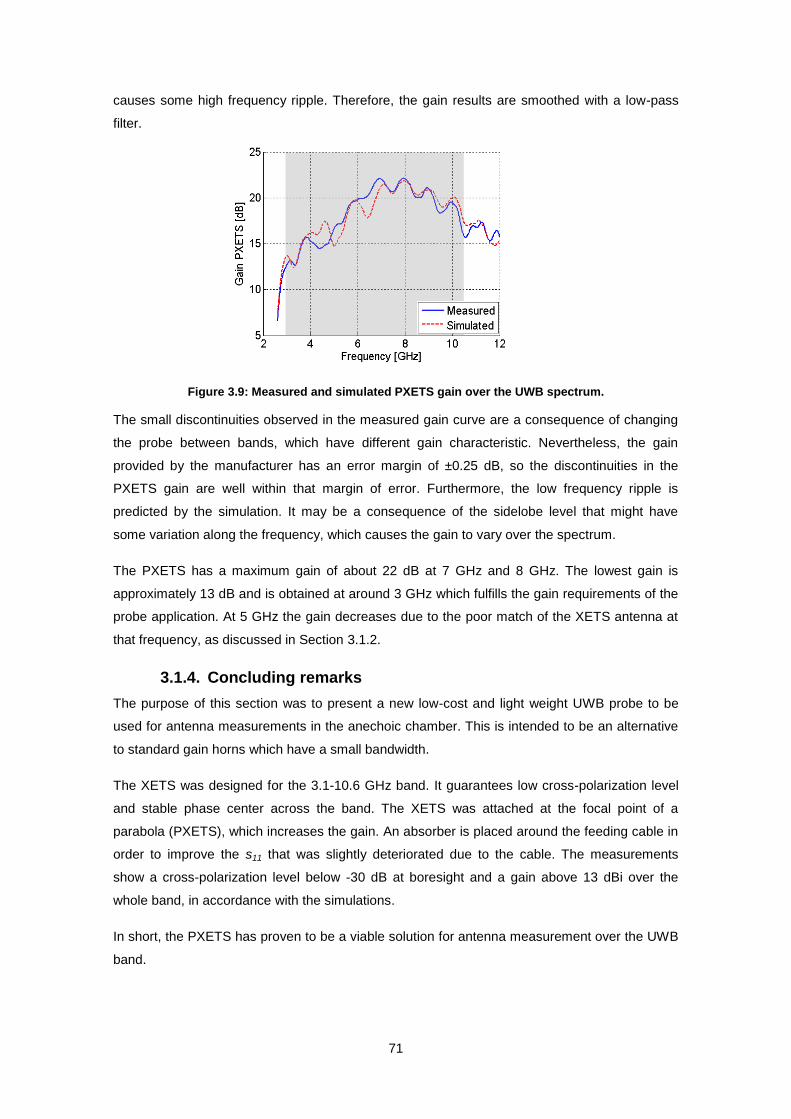
71
causes some high frequency ripple. Therefore, the gain results are smoothed with a low-pass
filter.
Figure 3.9: Measured and simulated PXETS gain over the UWB spectrum.
The small discontinuities observed in the measured gain curve are a consequence of changing
the probe between bands, which have different gain characteristic. Nevertheless, the gain
provided by the manufacturer has an error margin of ±0.25 dB, so the discontinuities in the
PXETS gain are well within that margin of error. Furthermore, the low frequency ripple is
predicted by the simulation. It may be a consequence of the sidelobe level that might have
some variation along the frequency, which causes the gain to vary over the spectrum.
The PXETS has a maximum gain of about 22 dB at 7 GHz and 8 GHz. The lowest gain is
approximately 13 dB and is obtained at around 3 GHz which fulfills the gain requirements of the
probe application. At 5 GHz the gain decreases due to the poor match of the XETS antenna at
that frequency, as discussed in Section 3.1.2.
3.1.4. Concluding remarks
The purpose of this section was to present a new low-cost and light weight UWB probe to be
used for antenna measurements in the anechoic chamber. This is intended to be an alternative
to standard gain horns which have a small bandwidth.
The XETS was designed for the 3.1-10.6 GHz band. It guarantees low cross-polarization level
and stable phase center across the band. The XETS was attached at the focal point of a
parabola (PXETS), which increases the gain. An absorber is placed around the feeding cable in
order to improve the s11 that was slightly deteriorated due to the cable. The measurements
show a cross-polarization level below -30 dB at boresight and a gain above 13 dBi over the
whole band, in accordance with the simulations.
In short, the PXETS has proven to be a viable solution for antenna measurement over the UWB
band.
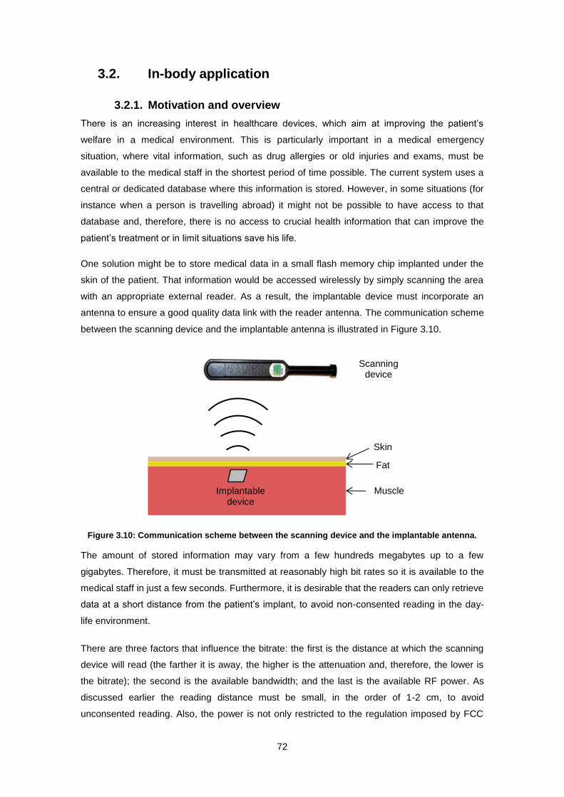
72
3.2. In-body application
3.2.1. Motivation and overview
There is an increasing interest in healthcare devices, which aim at improving the patient’s
welfare in a medical environment. This is particularly important in a medical emergency
situation, where vital information, such as drug allergies or old injuries and exams, must be
available to the medical staff in the shortest period of time possible. The current system uses a
central or dedicated database where this information is stored. However, in some situations (for
instance when a person is travelling abroad) it might not be possible to have access to that
database and, therefore, there is no access to crucial health information that can improve the
patient’s treatment or in limit situations save his life.
One solution might be to store medical data in a small flash memory chip implanted under the
skin of the patient. That information would be accessed wirelessly by simply scanning the area
with an appropriate external reader. As a result, the implantable device must incorporate an
antenna to ensure a good quality data link with the reader antenna. The communication scheme
between the scanning device and the implantable antenna is illustrated in Figure 3.10.
Figure 3.10: Communication scheme between the scanning device and the implantable antenna.
The amount of stored information may vary from a few hundreds megabytes up to a few
gigabytes. Therefore, it must be transmitted at reasonably high bit rates so it is available to the
medical staff in just a few seconds. Furthermore, it is desirable that the readers can only retrieve
data at a short distance from the patient’s implant, to avoid non-consented reading in the day-
life environment.
There are three factors that influence the bitrate: the first is the distance at which the scanning
device will read (the farther it is away, the higher is the attenuation and, therefore, the lower is
the bitrate); the second is the available bandwidth; and the last is the available RF power. As
discussed earlier the reading distance must be small, in the order of 1-2 cm, to avoid
unconsented reading. Also, the power is not only restricted to the regulation imposed by FCC
Implantable
device
Skin
Fat
Muscle
Scanning device
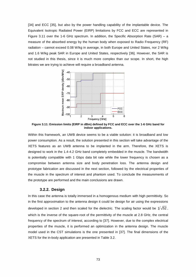
73
[34] and ECC [35], but also by the power handling capability of the implantable device. The
Equivalent Isotropic Radiated Power (EIRP) limitations by FCC and ECC are represented in
Figure 3.11 over the 1-6 GHz spectrum. In addition, the Specific Absorption Rate (SAR) – a
measure of the absorbed energy by the human body when exposed to Radio Frequency (RF)
radiation – cannot exceed 0.08 W/kg in average, in both Europe and United States, nor 2 W/kg
and 1.6 W/kg peak SAR in Europe and United States, respectively [36]. However, the SAR is
not studied in this thesis, since it is much more complex than our scope. In short, the high
bitrates we are trying to achieve will require a broadband antenna.
Figure 3.11: Emission limits (EIRP in dBm) defined by FCC and ECC over the 1-6 GHz band for indoor applications.
Within this framework, an UWB device seems to be a viable solution: it is broadband and low
power consumption. As a result, the solution presented in this section will take advantage of the
XETS features as an UWB antenna to be implanted in the arm. Therefore, the XETS is
designed to work in the 1.4-4.2 GHz band completely embedded in the muscle. The bandwidth
is potentially compatible with 1 Gbps data bit rate while the lower frequency is chosen as a
compromise between antenna size and body penetration loss. The antenna design and
prototype fabrication are discussed in the next section, followed by the electrical properties of
the muscle in the spectrum of interest and phantom used. To conclude the measurements of
the prototype are performed and the main conclusions are drawn.
3.2.2. Design
In this case the antenna is totally immersed in a homogenous medium with high permittivity. So
in the first approximation to the antenna design it could be design for air using the expressions
developed in section 2 and then scaled for the dielectric. The scaling factor would be 1 52 ,
which is the inverse of the square-root of the permittivity of the muscle at 2.8 GHz, the central
frequency of the spectrum of interest, according to [37]. However, due to the complex electrical
properties of the muscle, it is performed an optimization in the antenna design. The muscle
model used in the CST simulations is the one presented in [37]. The final dimensions of the
XETS for the in-body application are presented in Table 3.2.
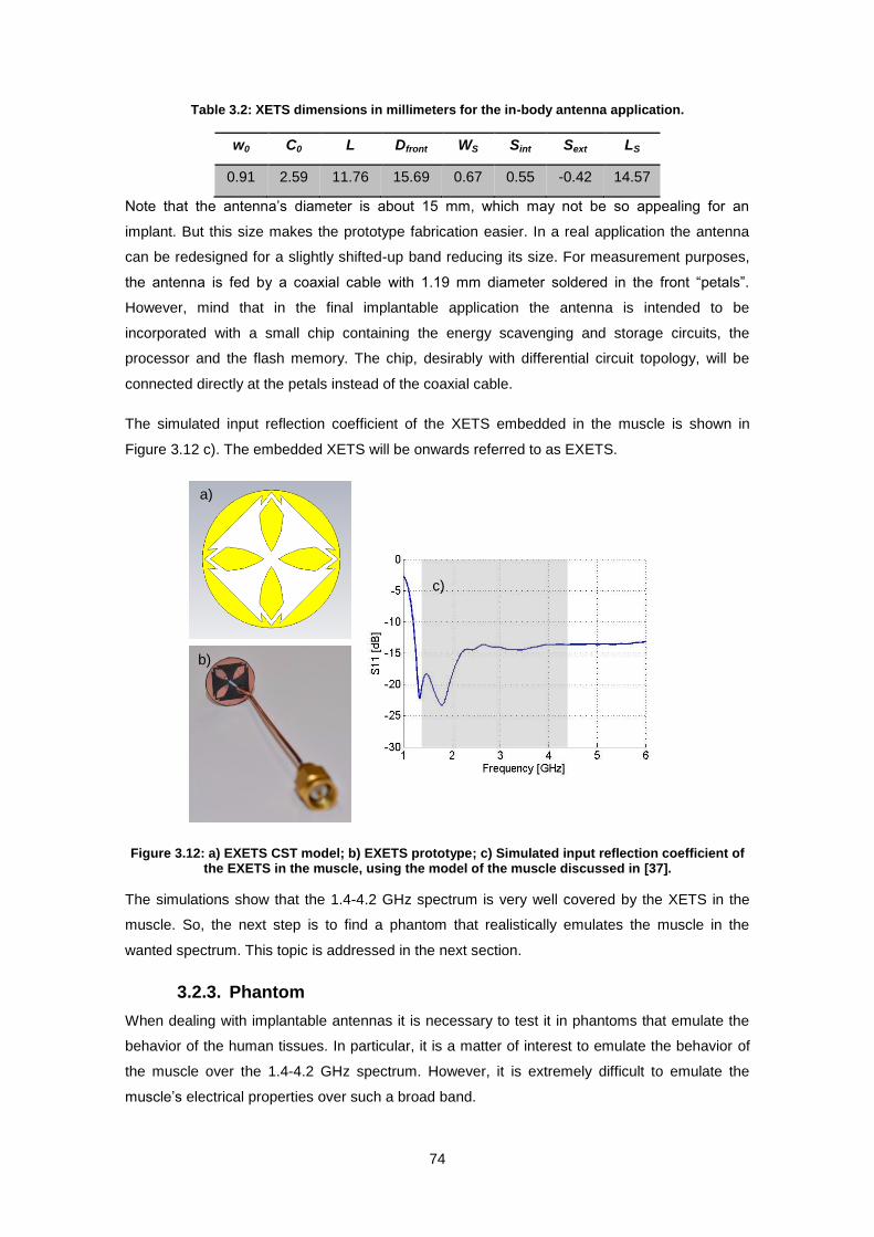
74
Table 3.2: XETS dimensions in millimeters for the in-body antenna application.
w0 C0 L Dfront WS Sint Sext LS
0.91 2.59 11.76 15.69 0.67 0.55 -0.42 14.57
Note that the antenna’s diameter is about 15 mm, which may not be so appealing for an
implant. But this size makes the prototype fabrication easier. In a real application the antenna
can be redesigned for a slightly shifted-up band reducing its size. For measurement purposes,
the antenna is fed by a coaxial cable with 1.19 mm diameter soldered in the front “petals”.
However, mind that in the final implantable application the antenna is intended to be
incorporated with a small chip containing the energy scavenging and storage circuits, the
processor and the flash memory. The chip, desirably with differential circuit topology, will be
connected directly at the petals instead of the coaxial cable.
The simulated input reflection coefficient of the XETS embedded in the muscle is shown in
Figure 3.12 c). The embedded XETS will be onwards referred to as EXETS.
Figure 3.12: a) EXETS CST model; b) EXETS prototype; c) Simulated input reflection coefficient of the EXETS in the muscle, using the model of the muscle discussed in [37].
The simulations show that the 1.4-4.2 GHz spectrum is very well covered by the XETS in the
muscle. So, the next step is to find a phantom that realistically emulates the muscle in the
wanted spectrum. This topic is addressed in the next section.
3.2.3. Phantom
When dealing with implantable antennas it is necessary to test it in phantoms that emulate the
behavior of the human tissues. In particular, it is a matter of interest to emulate the behavior of
the muscle over the 1.4-4.2 GHz spectrum. However, it is extremely difficult to emulate the
muscle’s electrical properties over such a broad band.
a)
b)
c)

75
According to [37], the human muscle presents a permittivity εr = 52 and a conductivity σ = 2 S/m
at 2.8 GHz. It is possible to find several different phantoms in the literature, depending on the
antenna usage, standard and location. A brief literature review on phantoms can be found in
[38], yet none covers the spectrum of interest. A solution could be to adjust other recipes, as the
one in [39], by increasing or diminishing the quantities of the solutes (sugar and NaCl salt), until
the wanted permittivity and conductivity are achieved. However, this method is very time
consuming besides being very difficult to achieve good results. Furthermore, it is not the
purpose of this work to develop a complex mixture to emulate the body behavior over such
band. As a result, the cheapest and quickest solution is to use the same recipe as the one used
before in [40], which is available in the IT laboratory.
Originally, the recipe was used to emulate the skin behavior in the 402-405 MHz band.
However, before using the phantom it is necessary to prove that it has similar electrical
properties to the muscle in the spectrum of interest. One way to characterize the phantom
electrical properties is to determine the corresponding physical model. The physical model that
best describes the electrical properties of aqueous composites is the Cole-Cole model, as
explained in [41].
According to the Cole-Cole model the complex permittivity ε* is described by
1
0
* ' ''1
sjjj
(70)
where ω is the angular frequency, τ is the relaxation time, σ is the conductivity and εs and ε∞ are
the static and infinite frequency dielectric constants, respectively [41]. So, to describe the
phantom it is necessary to determine all these values.
To do so, it is used a reflection- and transmission-based method described in [40] and [42] that
was proven to be reasonably accurate, as seen in annex A.3. It consists of a metal container
crossed from side to side by the inner conductor of a coaxial cable. Since the working frequency
is much higher than the one used in [40] and [42], there was the need to fabricating a smaller
container, as illustrated by Figure 3.13 with a volume 20.2 × 20 × 7 mm3.
Figure 3.13: Container for complex permittivity measurements of liquid materials.
The cavity is filled with the phantom liquid and the dispersion matrix is measured. The
measurements results are represented by the blue curve in Figure 3.14 and Figure 3.15. The
Cole-Cole parameters are achieved by trial and error by comparing the measurements with the

76
simulation results. In the CST simulation mode, the Cole-Cole model is selected, in which
different values of the parameters are tested until there is a good match between the simulation
and the measurements results. The achieved values are presented in Table 3.3.
Table 3.3: Cole-Cole parameters of the measured phantom model.
τ [ps] ε∞ εs σ [S/m] α
42.35 5 60 0.2 0.07
The simulated results are represented by the red curve in Figure 3.14 and Figure 3.15.
Figure 3.14: Container filled with the phantom liquid: a) input reflection coefficient, s11; b) unwrapped phase of the reflection coefficient.
Figure 3.15: Container filled with the phantom liquid: a) transmission coefficient, s21; b) unwrapped phase of the transmission coefficient.
The results exhibit good match between the measured and simulated results, which means that
the phantom is well characterized by the determined Cole-Cole model.
Once the Cole-Cole model is determined it is possible to study how the permittivity varies along
the frequency. As seen before in (70), the complex permittivity can be separated into real and
imaginary parts. The real part represents the permittivity, whereas the imaginary part allows
calculating the losses, by calculating the tangent of the ratio between the imaginary and the real
parts. Figure 3.16 illustrates how the permittivity of the Cole-Cole model varies along the
frequency, compared to the muscle’s electrical properties.
a) b)
a) b)

77
Figure 3.16: Permittivity variation along the frequency, using the determined Cole-Cole model and the muscle´s electrical properties described in [37].
At 2.8 GHz the liquid presents a permittivity εr of 40, approximately, which is a bit lower than the
muscle’s permittivity [37]. However it is not completely unreasonable, which makes us consider
this liquid as a valid phantom. The conductivity is assumed to be constant along the band as
described in [41], which is not entirely true. Yet, the conductivity value is the one shown in Table
3.3.
It is now relevant to understand how the XETS performs over the 1.4-4.2 GHz spectrum, using
the phantom model. Therefore the reflection coefficient was simulated, as shown in Figure 3.17,
when the antenna is immersed in the muscle model described in [37] and in the Cole-Cole.
Figure 3.17: Simulated input reflection coefficients in CST using the muscle model discussed in [37] and the model of the phantom in the IT laboratory.
The results show that the antenna performance is hardly affected by the differences between
the two phantom models. In both cases the antenna bandwidth is preserved.
3.2.4. Measurement of the electromagnetic performance
This section presents the XETS prototype measurements and compares it to the expected
results using the liquid phantom model described in the previous section. To measure the
prototype’s reflection coefficient the antenna is immersed in the phantom liquid inside a plastic
cup, as shown in Figure 3.18 a). It can be shown that the shape of the cup affects marginally
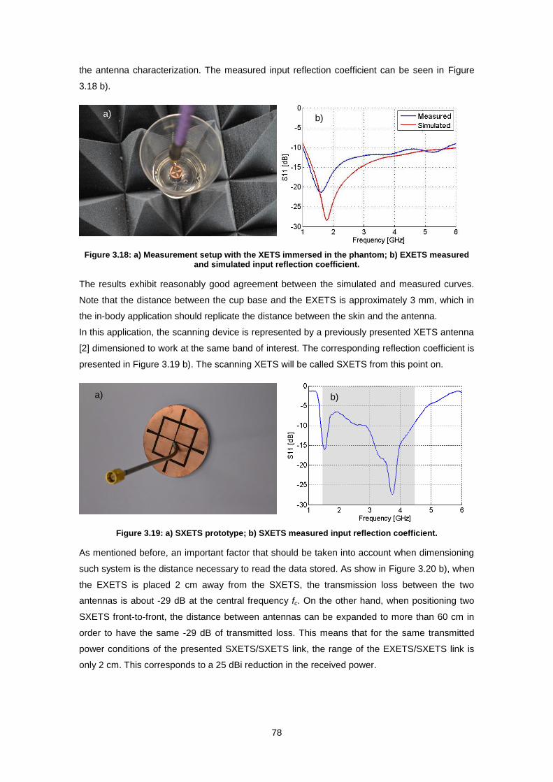
78
the antenna characterization. The measured input reflection coefficient can be seen in Figure
3.18 b).
Figure 3.18: a) Measurement setup with the XETS immersed in the phantom; b) EXETS measured and simulated input reflection coefficient.
The results exhibit reasonably good agreement between the simulated and measured curves.
Note that the distance between the cup base and the EXETS is approximately 3 mm, which in
the in-body application should replicate the distance between the skin and the antenna.
In this application, the scanning device is represented by a previously presented XETS antenna
[2] dimensioned to work at the same band of interest. The corresponding reflection coefficient is
presented in Figure 3.19 b). The scanning XETS will be called SXETS from this point on.
Figure 3.19: a) SXETS prototype; b) SXETS measured input reflection coefficient.
As mentioned before, an important factor that should be taken into account when dimensioning
such system is the distance necessary to read the data stored. As show in Figure 3.20 b), when
the EXETS is placed 2 cm away from the SXETS, the transmission loss between the two
antennas is about -29 dB at the central frequency fc. On the other hand, when positioning two
SXETS front-to-front, the distance between antennas can be expanded to more than 60 cm in
order to have the same -29 dB of transmitted loss. This means that for the same transmitted
power conditions of the presented SXETS/SXETS link, the range of the EXETS/SXETS link is
only 2 cm. This corresponds to a 25 dBi reduction in the received power.
a) b)
a) b)

79
Figure 3.20: a) Measurement setup; b) transmission coefficient as a function of the distance.
3.2.5. Data transmission performance
The purpose of the EXETS is to transmit the patient’s health information from the implanted
mass storage device to the external scanning device. The amount of information can get to a
few gigabytes and the intended scanning time is in the order of only a few seconds. Therefore,
to transmit such an amount of information in a short lapse of time it is necessary to reach high
bitrates, at least in the order of hundreds of Mbps.
The achievable gross bitrate is related to the pulse distortion that the antenna introduces in the
transmission of a pulse, or in other words it is related to the antenna pulse fidelity. To analyze
the fidelity a Gaussian pulse is adopted as defined in (21), where the central frequency is fc =
2.8 GHz and the Gaussian width is τ = 850 ps. The fidelity over the solid angle is shown in
Figure 3.21 a). It can be seen that there is almost no pulse distortion, which is a very good
indicator.
Figure 3.21: a) Fidelity of the EXETS over the solid angle; b) Time window containing 90% of the pulse energy transmitted by the EXETS over the solid angle (the E90 window for the input pulse is
0.56 ns). The radial angle is theta and the polar angle is phi.
EXETS
SXETS
a)
b)
a) b)
[ns] %
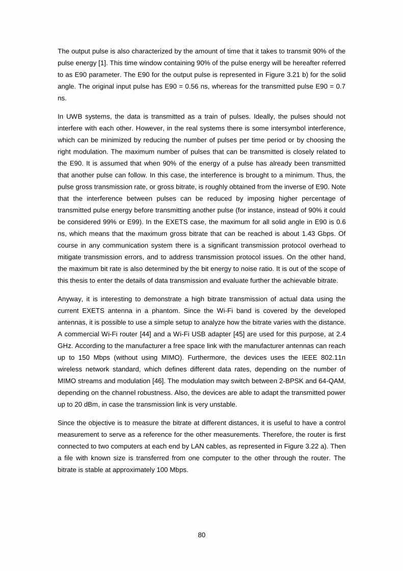
80
The output pulse is also characterized by the amount of time that it takes to transmit 90% of the
pulse energy [1]. This time window containing 90% of the pulse energy will be hereafter referred
to as E90 parameter. The E90 for the output pulse is represented in Figure 3.21 b) for the solid
angle. The original input pulse has E90 = 0.56 ns, whereas for the transmitted pulse E90 = 0.7
ns.
In UWB systems, the data is transmitted as a train of pulses. Ideally, the pulses should not
interfere with each other. However, in the real systems there is some intersymbol interference,
which can be minimized by reducing the number of pulses per time period or by choosing the
right modulation. The maximum number of pulses that can be transmitted is closely related to
the E90. It is assumed that when 90% of the energy of a pulse has already been transmitted
that another pulse can follow. In this case, the interference is brought to a minimum. Thus, the
pulse gross transmission rate, or gross bitrate, is roughly obtained from the inverse of E90. Note
that the interference between pulses can be reduced by imposing higher percentage of
transmitted pulse energy before transmitting another pulse (for instance, instead of 90% it could
be considered 99% or E99). In the EXETS case, the maximum for all solid angle in E90 is 0.6
ns, which means that the maximum gross bitrate that can be reached is about 1.43 Gbps. Of
course in any communication system there is a significant transmission protocol overhead to
mitigate transmission errors, and to address transmission protocol issues. On the other hand,
the maximum bit rate is also determined by the bit energy to noise ratio. It is out of the scope of
this thesis to enter the details of data transmission and evaluate further the achievable bitrate.
Anyway, it is interesting to demonstrate a high bitrate transmission of actual data using the
current EXETS antenna in a phantom. Since the Wi-Fi band is covered by the developed
antennas, it is possible to use a simple setup to analyze how the bitrate varies with the distance.
A commercial Wi-Fi router [44] and a Wi-Fi USB adapter [45] are used for this purpose, at 2.4
GHz. According to the manufacturer a free space link with the manufacturer antennas can reach
up to 150 Mbps (without using MIMO). Furthermore, the devices uses the IEEE 802.11n
wireless network standard, which defines different data rates, depending on the number of
MIMO streams and modulation [46]. The modulation may switch between 2-BPSK and 64-QAM,
depending on the channel robustness. Also, the devices are able to adapt the transmitted power
up to 20 dBm, in case the transmission link is very unstable.
Since the objective is to measure the bitrate at different distances, it is useful to have a control
measurement to serve as a reference for the other measurements. Therefore, the router is first
connected to two computers at each end by LAN cables, as represented in Figure 3.22 a). Then
a file with known size is transferred from one computer to the other through the router. The
bitrate is stable at approximately 100 Mbps.

81
Figure 3.22: Experiment setup schemes using the router.
The router’s antenna is then replaced by the SXETS which is positioned front-to-front with the
USB adapter. Both devices are connected to two different computers. The same file that was
previously used is now transferred from one computer to the other using the link between the
antennas. The transfer time and instant bitrate are controlled in one of the computers. This
situation is represented by case b) in Figure 3.22. This process is repeated for different distance
values between the antennas.
At last, the SXETS is replaced by the EXETS immersed in the phantom. The file is repeatedly
transferred from one computer to the other at different distances using the transmission link.
The transfer time and instant bitrate are accounted again. This setup is represented by c) in
Figure 3.22.
The experimental setup at the IT laboratory and the obtained results are shown in Figure 3.23
a) and b), respectively. The graphic shows the average bitrate Ravg (which was calculated as the
ratio between the file size and the transfer time) and the peak bitrate Rpeak (the maximum instant
bitrate achieved). These indicators are shown for the both situations using SXETS and EXETS.
Using the SXETS as the transmission antenna the average bitrate is stable at around 90 Mbps
whereas the peak is approximately 100 Mbps, except near 50 mm. At this distance the SXETS
is very close to the USB adapter and the circuits couple with each other, which explains the
lower bitrate. In spite of that at larger distances the peak bitrate matches the one obtained using
a cable which is very good. When the SXETS is replaced by the EXETS immersed in the liquid,
it is verified that the bitrate decreases substantially with the distance and Ravg stabilizes at 35
Mbps. At 20 mm (the intended reader distance in the final application) the bitrate reaches the
same typical values obtained for the SXETS with Rpeak = 99 Mbps and Ravg = 87 Mbps.
LAN cable LAN cable
a)
LAN cable
SXETS
Wi-Fi USB adapter
b)
LAN cable
EXETS immersed in the phantom
Wi-Fi USB adapter
c)
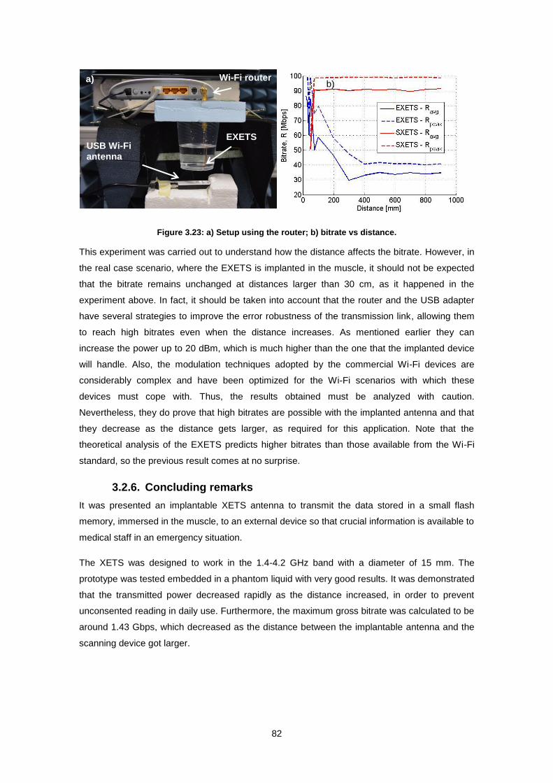
82
Figure 3.23: a) Setup using the router; b) bitrate vs distance.
This experiment was carried out to understand how the distance affects the bitrate. However, in
the real case scenario, where the EXETS is implanted in the muscle, it should not be expected
that the bitrate remains unchanged at distances larger than 30 cm, as it happened in the
experiment above. In fact, it should be taken into account that the router and the USB adapter
have several strategies to improve the error robustness of the transmission link, allowing them
to reach high bitrates even when the distance increases. As mentioned earlier they can
increase the power up to 20 dBm, which is much higher than the one that the implanted device
will handle. Also, the modulation techniques adopted by the commercial Wi-Fi devices are
considerably complex and have been optimized for the Wi-Fi scenarios with which these
devices must cope with. Thus, the results obtained must be analyzed with caution.
Nevertheless, they do prove that high bitrates are possible with the implanted antenna and that
they decrease as the distance gets larger, as required for this application. Note that the
theoretical analysis of the EXETS predicts higher bitrates than those available from the Wi-Fi
standard, so the previous result comes at no surprise.
3.2.6. Concluding remarks
It was presented an implantable XETS antenna to transmit the data stored in a small flash
memory, immersed in the muscle, to an external device so that crucial information is available to
medical staff in an emergency situation.
The XETS was designed to work in the 1.4-4.2 GHz band with a diameter of 15 mm. The
prototype was tested embedded in a phantom liquid with very good results. It was demonstrated
that the transmitted power decreased rapidly as the distance increased, in order to prevent
unconsented reading in daily use. Furthermore, the maximum gross bitrate was calculated to be
around 1.43 Gbps, which decreased as the distance between the implantable antenna and the
scanning device got larger.
Wi-Fi router
EXETS USB Wi-Fi antenna
a) b)

83
4. Conclusions and Future work
4.1. Conclusions
The first part of this work addressed the complete study of the XETS antenna developed at IT.
Before the present study, the XETS antenna design was based on full-wave simulations which
was very time consuming and difficult to perform, since the antenna’s geometry is very complex.
Now, by making use of the expressions determined in this work, it becomes very quick and
simple to get a first approximation of the antenna design.
A thorough methodology was followed, in order to guarantee that the results were accurate and
repeatable. The approach consisted in separating the metal antenna design from the substrate
effects. As a result, the antenna was analyzed as a simple metal layer that is easily scalable
with the frequency. Still with an antenna without substrate, it was studied how the XETS could
be designed to cover an arbitrary bandwidth ratio up to 3:1. Once these expressions were
determined and tested, the dielectric substrate was introduced. The substrate effects were quite
difficult to predict. Consequently, the strategy was to adapt to the XETS antenna the well-known
effective permittivity concept used for microstrip lines, although the XETS physics is much more
complex than the classical microstrip line. A model of the effective permittivity was proposed
and determined with very good results. A small optimization process was then performed in
order to improve the final results. After analyzing the validity of the model, three different
examples were presented which show that the expressions determined give, in fact, a very
good first approximation of the XETS design.
Two practical applications of the XETS and of the proposed design methodology were also
presented. The first test case was the design of a ultrawide band probe for anechoic chamber
measurements, based on the XETS. This ultrawide band probe is useful to replace the
traditional need for four different standard gain horn antennas to cover such a broad band,
which is a rather tedious process. The new probe takes advantage of the XETS low cross
polarization level and stable phase center. The XETS was designed using the expressions
determined before. To increase the antenna gain, the XETS was integrated with a 35 cm
diameter parabolic reflector. The XETS is located at the parabola focal point at 14.5 cm from the
parabola apex. The long coaxial cable needed to feed the XETS tends to deteriorate the input
reflection coefficient. As a result, an absorber is included that slightly improves the antenna’s
performance. The radiation patterns of the prototype exhibit a very well defined main lobe with a
cross-polarization level below -15 dB over the whole spectrum. Furthermore, the measured gain
was 22 dBi at 7 GHz and 8 GHz and it was above 13 dBi within the UWB band, which match the
simulation results. The main drawback of this solution is its size, which requires a relatively
large anechoic chamber in order to meet the farfield measurement condition.
An additional application was presented, in which the XETS must be implanted in the muscle.
The objective is to integrate the antenna with a storage device that gathers key health

84
information about the patient. The antenna is used to transmit the data from the implanted
device to an external scanning instrument. So, a XETS was designed to work over the 1.4-4.2
GHz spectrum while embedded in a medium with the electromagnetic properties of the body,
based on the expressions determined in the first part of this work. A prototype was fabricated
and demonstrated experimentally. To emulate the human body electrical properties, a liquid
phantom was used, following a recipe used in previous works for the MedRadio 402-405 MHz
band. Although not completely different, the electrical properties of the phantom do not entirely
match the human body properties over the UWB spectrum of interest. However, it was shown
that the antenna performance did not suffer major modification when immersed in different
phantom formulas, as confirmed by the measured input reflection coefficient. Developing a
phantom for the UWB band was out of the scope this work. The results of the analysis showed
that the XETS can reach up to 1.43 Gbps bitrate, which is an extremely promising result given
the gigabytes of information that are envisaged to be stored in the device. Furthermore, it was
proven that the optimal distance at which the scanning device must be placed to read the
information is between 20 mm up to 40 mm. This fact minimizes unconsented reading by alien
devices.

85
4.2. Future work
It is intended to integrate the XETS design calculator in the Antenna Magus database, so that it
becomes easily available to the antenna community. Thus, any developer can design the XETS
antenna according to his specifications and develop new applications for this antenna.
Regarding the in-body application, new phantom recipes should be taken into account, in order
to better emulate the muscle’s electrical properties. This way, the embedded XETS can be more
realistically tested. In particular, it should be studied in more detail the SAR in order to verify
that the FCC and ECC limits are complied. In addition to this, it is required a further analysis of
the bitrate, so that it is fully characterized. In fact, the maximum bitrate is also determined by the
bit energy, which was not analyzed in this thesis. At last, it is intended to create an application
for the embedded XETS in order to motivate and demonstrate the potential of this application to
other students and researchers.

86
87
5. References
[1] Jorge R. Costa, Carla R. Medeiros and Carlos A. Fernandes, “Performance of a Crossed
Exponentially Tapered Slot Antenna for UWB Systems,” IEEE Transactions on Antennas
and Propagation, vol. 57, no. 5, pp. 1345-1352, May 2009.
[2] Jorge R. Costa and Carlos A. Fernandes, “Broadband Slot Feed for Integrated Lens
Antenna,” IEEE Antennas and Wireless Propagation Letters, vol. 6, 2007.
[3] Carla R. Medeiros, Eduardo B. Lima, Jorge R. Costa and Carlos A. Fernandes, “Wideband
Slot Antenna for WLAN Access Points,” IEEE Antennas and Wireless Propagation Letters,
vol. 9, 2010.
[4] Jorge R. Costa, Eduardo B. Lima, Carla R. Medeiros and Carlos A. Fernandes, “Evaluation
of a New Wideband Slot Array for MIMO Performance Enhancement in Indoor WLANs,”
IEEE Transactions on Antennas and Propagation, vol. 59, no. 4, April, 2011.
[5] Carla R. Medeiros, Jorge R. Costa and Carlos A. Fernandes, “Compact Tapered Slot UWB
Antenna With WLAN Band Rejection,” IEEE Antennas and Wireless Propagation Letters,
vol. 8, 2009.
[6] Catarina C. Cruz, Jorge R. Costa, Carlos A. Fernandes, “Hybrid UHF/UWB Antenna for
Passive Indoor Identification and Localization Systems,” IEEE Transactions on Antennas
and Propagation, vol. 61, no. 1, Jan. 2013.
[7] C. K. Campbell, I. Traboulay, M. S. Suthers and H. Kneve, “Design of a Stripline Log-
periodic Dipole Antenna,” IEEE Transactions Antennas Propagation, vol. AP-25, no. 5, pp.
718-721, Sep. 1977.
[8] P. J. Gibson, “The Vivaldi Aerial,” 9th European Microwave Conference, Brighton, England,
Sep. 1979.
[9] Tutku Karacolak and Erdem Topsakal, “A Double-Sided Rounded Bow-Tie Antenna
(DSRBA) for UWB Communication,” IEEE Antennas and Wireless Propagation Letters, vol.
5, no. 1, pp. 446-449, Dec. 2006.
[10] T. E. Morgan, “Reduced Size Spiral Antenna,” 9th European Microwave Conference,
Brighton, England, Sep. 1979.
[11] J. Liang, C. C. Chiau, X. Chen and C. G. Parini, “Study of a Printed Circular Disc Monopole
Antenna for UWB Systems,” IEEE Transactions on Antennas and Propagation, vol. 53, no.
11, pp. 3500-3504, Nov. 2005.
[12] X. Chen, J. Liang, P. Li, L. Guo, C. C. Chiau and C. G. Parini, “Planar UWB monopole
Antennas,” Microwave Conference Proceedings, APMC 2005, Asia-Pacific Conference
Proceedings, Dec. 2005.
[13] E. Guéguen, F. Thudor, P. Chambelin, “A Low Cost UWB Printed Dipole Antenna with High
Performances,” in Procedures IEEE International Conference on Ultra-Wideband-ICU 2005,
Zurich, Switzerland, pp. 89-92, Sep. 2005.

88
[14] Taeyoung Yamg, Seong-Youp Suh, Randall Nealy, et al., “Compact Planar Antenna for
UWB Applications,” on International Conference Microwave and Millimeter Wave
Technology (ICMMT), pp. 1987-1990, May 2010.
[15] F. Liu, K. L. Lau, Q. Xue and C. H. Chan, “Experimental Studies of Printed Wide-Slot
Antenna for Wide-Band Applications,” IEEE Antennas and Wireless Propagations Letters,
vol. 3, pp. 273-275, Dec. 2004.
[16] Hadi Bahrami, Benoit Gosselin and Leslie A. Rusch, “Design of a miniaturized UWB
antenna optimized for implantable neural recordings systems,” IEEE 10th International New
Circuits and Systems Conference (NEWCAS), pp. 309-312, June 2012.
[17] Sinan Gezigi and H. Vincent Poor, “Position Estimation via Ultra-Wide-Band Signals,”
Proceedings IEEE, vol. 97, no. 2, pp. 386-403, Feb. 2009.
[18] Sinan Gezigi, Zhi Tian, Georgios B. Giannakis, Hisashi Kobayashi, Andreas F. Molisch, H.
Vincent Poor, and Zafer Sahinoglu, “Localization via Ultra-Wideband Radios,” IEEE Signal
Processing Magazine, vol. 22, no. 4, pp. 70-84, 2005.
[19] ETS-Lindgren, “Double Ridged Waveguide Horn”, Model 3117 datasheet.
[20] Millimeter Wave Technology & Solutions, “Standard Gain Conical and Pyramidal Horns”,
Series SGH datasheet.
[21] Millimeter Wave Products Inc., “Standard Gain Horns”, 261 Series datasheet.
[22] Satimo, “Standard Gain Horns”, Measurement antennas datasheet.
[23] TDK, “Horn Antenna”, HRN-0118 datasheet, Rev. 2012-09-10.
[24] J. L. Kerr, “Short axial length broad-band horns,” IEEE Transactions on Antenna
Propagation, vol. 21, no. 5, pp. 710-714, Sep. 1973.
[25] A. Giocomini, A. Potenza, R. Morbidini and L. Foged, “Quad-ridge Dual Polarized Antenna
for Use in the 2-32 GHz Band,” 6th European Conference on Antenna and Propagation
(EUCAP), Prague, March 2012.
[26] Bennie. Jacobs, Johann W. Odendaal and Johan Joubert, “An Improved Design for a 1-18
GHz Double-Ridged Guide Horn Antenna”, IEEE Transactions on Antenna and
Propagation, vol. 60, no. 9, Sep. 2012.
[27] CST – Computer Simulation Technology, https://www.cst.com/, 2014.
[28] David M. Pozar, Microwave Engineering, John Wiley & Sons, Inc., 3rd
edition, 2005, ch. 3,
sec. 8, pp. 143-146.
[29] Rogers Corporation, “RT/duroid 5870/5880 High Frequency Laminates”, duroid 5870/5880
datasheet.
[30] Rogers Corporation, “RT/duroid 6002 High Frequency Laminates”, duroid 6002 datasheet.
[31] Rogers Corporation, “RT/duroid 6035HTC High Frequency Laminates”, duroid 6035HTC
datasheet.
[32] ventecUSA, “VT-42 Datasheets”, VT-42 CCL/Laminate VT-42 PP/Prepreg datasheet,
issued Oct. 2011.
[33] Antenna Magus, http://www.antennamagus.com, 2014.
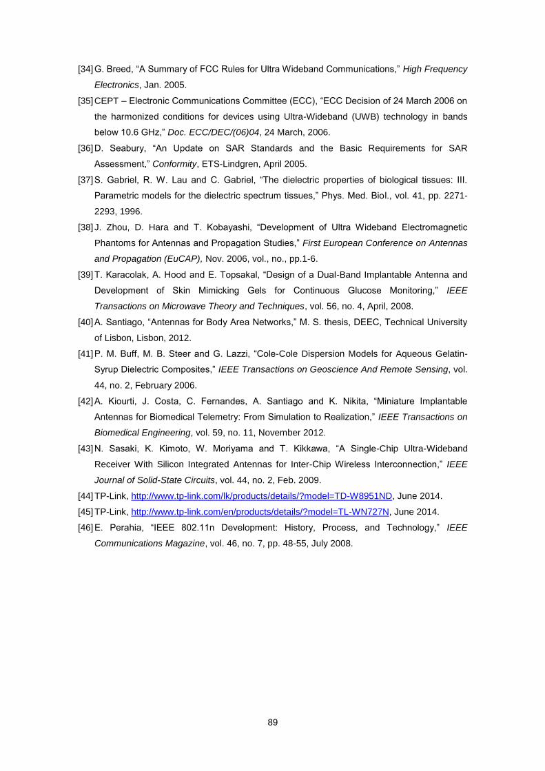
89
[34] G. Breed, “A Summary of FCC Rules for Ultra Wideband Communications,” High Frequency
Electronics, Jan. 2005.
[35] CEPT – Electronic Communications Committee (ECC), “ECC Decision of 24 March 2006 on
the harmonized conditions for devices using Ultra-Wideband (UWB) technology in bands
below 10.6 GHz,” Doc. ECC/DEC/(06)04, 24 March, 2006.
[36] D. Seabury, “An Update on SAR Standards and the Basic Requirements for SAR
Assessment,” Conformity, ETS-Lindgren, April 2005.
[37] S. Gabriel, R. W. Lau and C. Gabriel, “The dielectric properties of biological tissues: III.
Parametric models for the dielectric spectrum tissues,” Phys. Med. Biol., vol. 41, pp. 2271-
2293, 1996.
[38] J. Zhou, D. Hara and T. Kobayashi, “Development of Ultra Wideband Electromagnetic
Phantoms for Antennas and Propagation Studies,” First European Conference on Antennas
and Propagation (EuCAP), Nov. 2006, vol., no., pp.1-6.
[39] T. Karacolak, A. Hood and E. Topsakal, “Design of a Dual-Band Implantable Antenna and
Development of Skin Mimicking Gels for Continuous Glucose Monitoring,” IEEE
Transactions on Microwave Theory and Techniques, vol. 56, no. 4, April, 2008.
[40] A. Santiago, “Antennas for Body Area Networks,” M. S. thesis, DEEC, Technical University
of Lisbon, Lisbon, 2012.
[41] P. M. Buff, M. B. Steer and G. Lazzi, “Cole-Cole Dispersion Models for Aqueous Gelatin-
Syrup Dielectric Composites,” IEEE Transactions on Geoscience And Remote Sensing, vol.
44, no. 2, February 2006.
[42] A. Kiourti, J. Costa, C. Fernandes, A. Santiago and K. Nikita, “Miniature Implantable
Antennas for Biomedical Telemetry: From Simulation to Realization,” IEEE Transactions on
Biomedical Engineering, vol. 59, no. 11, November 2012.
[43] N. Sasaki, K. Kimoto, W. Moriyama and T. Kikkawa, “A Single-Chip Ultra-Wideband
Receiver With Silicon Integrated Antennas for Inter-Chip Wireless Interconnection,” IEEE
Journal of Solid-State Circuits, vol. 44, no. 2, Feb. 2009.
[44] TP-Link, http://www.tp-link.com/lk/products/details/?model=TD-W8951ND, June 2014.
[45] TP-Link, http://www.tp-link.com/en/products/details/?model=TL-WN727N, June 2014.
[46] E. Perahia, “IEEE 802.11n Development: History, Process, and Technology,” IEEE
Communications Magazine, vol. 46, no. 7, pp. 48-55, July 2008.

90
A. Annexes
A.1. Effective permittivity estimation
In this Annex, it is presented the graphics of the effective permittivity for BWR = 2.16 and 1.56,
as discussed in sections 2.3.1.4 and 2.3.1.5, respectively. The blue dots represent the effective
permittivity values calculated through the scale factors ScF, the red line is the best-fitting curve
using the XETS effective permittivity model and the dashed blue line is the effective permittivity
curve obtained using the expressions determined the corresponding sections.
Within each BWR, it is presented a total number of 23 graphs, categorized in four figures
according to the substrate permittivity εr. Each graph provides a value of b and d that is used in
section 2.3 to determine the corresponding expressions.
A.1.1 BWR = 2.16
This sub-section presents the effective permittivity graphs for BWR = 2.16 as a function of
thickness in millimeters. Mind that for εr = 3.5 there are only five graphs because at fL = 32.675
GHz it is not possible to determine the ScF since the model falls out of validity.
As observed in Figure A.1 - Figure A.4, there is a reasonable agreement between the best-
fitting curve (red line) and the curve obtained through the final expressions of the XETS
effective permittivity model (dashed blue curve).
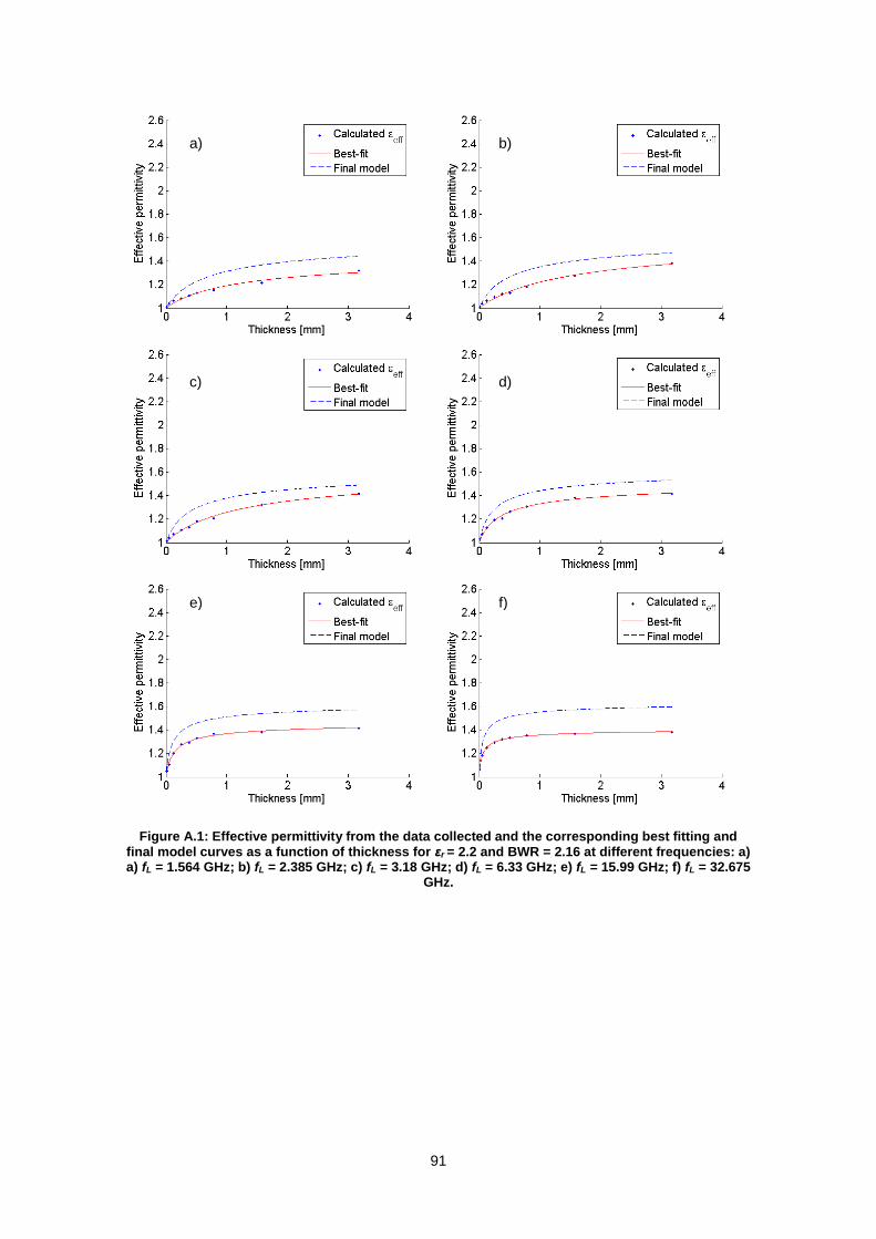
91
Figure A.1: Effective permittivity from the data collected and the corresponding best fitting and final model curves as a function of thickness for εr = 2.2 and BWR = 2.16 at different frequencies: a) a) fL = 1.564 GHz; b) fL = 2.385 GHz; c) fL = 3.18 GHz; d) fL = 6.33 GHz; e) fL = 15.99 GHz; f) fL = 32.675
GHz.
a) b)
c) d)
e) f)
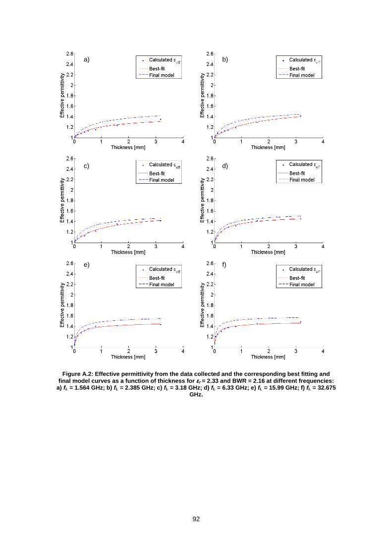
92
Figure A.2: Effective permittivity from the data collected and the corresponding best fitting and final model curves as a function of thickness for εr = 2.33 and BWR = 2.16 at different frequencies:
a) fL = 1.564 GHz; b) fL = 2.385 GHz; c) fL = 3.18 GHz; d) fL = 6.33 GHz; e) fL = 15.99 GHz; f) fL = 32.675 GHz.
a) b)
c) d)
e) f)
93
Figure A.3: Effective permittivity from the data collected and the corresponding best fitting and final model curves as a function of thickness for εr = 2.94 and BWR = 2.16 at different frequencies:
a) fL = 1.564 GHz; b) fL = 2.385 GHz; c) fL = 3.18 GHz; d) fL = 6.33 GHz; e) fL = 15.99 GHz; f) fL = 32.675 GHz.
a) b)
c) d)
e) f)
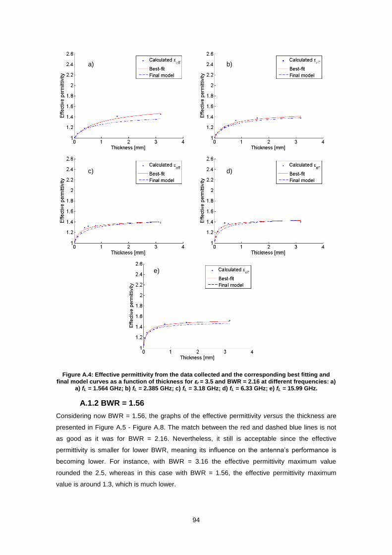
94
Figure A.4: Effective permittivity from the data collected and the corresponding best fitting and final model curves as a function of thickness for εr = 3.5 and BWR = 2.16 at different frequencies: a)
a) fL = 1.564 GHz; b) fL = 2.385 GHz; c) fL = 3.18 GHz; d) fL = 6.33 GHz; e) fL = 15.99 GHz.
A.1.2 BWR = 1.56
Considering now BWR = 1.56, the graphs of the effective permittivity versus the thickness are
presented in Figure A.5 - Figure A.8. The match between the red and dashed blue lines is not
as good as it was for BWR = 2.16. Nevertheless, it still is acceptable since the effective
permittivity is smaller for lower BWR, meaning its influence on the antenna’s performance is
becoming lower. For instance, with BWR = 3.16 the effective permittivity maximum value
rounded the 2.5, whereas in this case with BWR = 1.56, the effective permittivity maximum
value is around 1.3, which is much lower.
a) b)
c) d)
e)

95
Figure A.5: Effective permittivity from the data collected and the corresponding best fitting and final model curves as a function of thickness for εr = 2.2 and BWR = 1.56 at different frequencies: a)
fL = 1.564 GHz; b) fL = 2.385 GHz; c) fL = 3.18 GHz; d) fL = 6.33 GHz; e) fL = 15.99 GHz; f) fL = 32.675 GHz.
a) b)
c) d)
e) f)

96
Figure A.6: Effective permittivity from the data collected and the corresponding best fitting and final model curves as a function of thickness for εr = 2.33 and BWR = 1.56 at different frequencies:
a) fL = 1.564 GHz; b) fL = 2.385 GHz; c) fL = 3.18 GHz; d) fL = 6.33 GHz; e) fL = 15.99 GHz; f) fL = 32.675 GHz.
a) b)
c) d)
e) f)
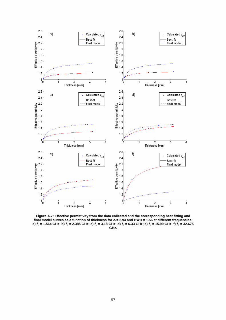
97
Figure A.7: Effective permittivity from the data collected and the corresponding best fitting and final model curves as a function of thickness for εr = 2.94 and BWR = 1.56 at different frequencies:
a) fL = 1.564 GHz; b) fL = 2.385 GHz; c) fL = 3.18 GHz; d) fL = 6.33 GHz; e) fL = 15.99 GHz; f) fL = 32.675 GHz.
a) b)
c) d)
e) f)
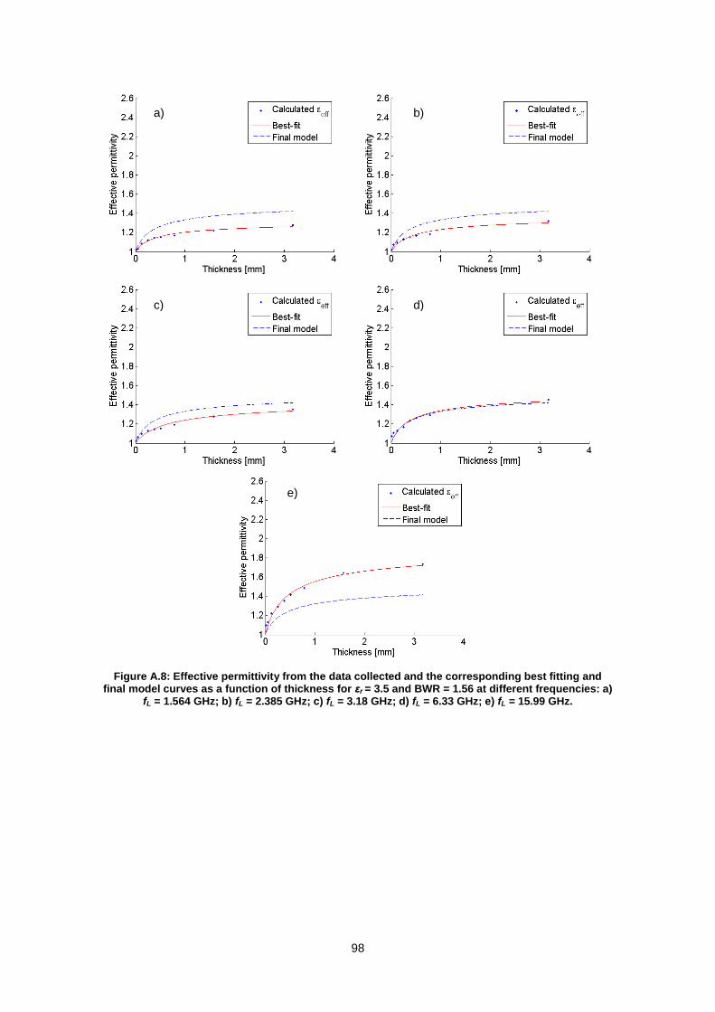
98
Figure A.8: Effective permittivity from the data collected and the corresponding best fitting and final model curves as a function of thickness for εr = 3.5 and BWR = 1.56 at different frequencies: a)
fL = 1.564 GHz; b) fL = 2.385 GHz; c) fL = 3.18 GHz; d) fL = 6.33 GHz; e) fL = 15.99 GHz.
a) b)
c) d)
e)

99
A.2. Styrofoam’s permittivity measurement
In order to determine the styrofoam’s permittivity, a technique based on transmission
measurements is performed. The physical principal of this experiment is that the styrofoam
introduces a phase delay, compared to the unobstructed link, which allows calculating the
refractive index, as follows.
0 0k l k nl
0 1k l n
2 2
1360
l n
1360
l
n (A.1)
where k0 is the propagation constant in air, l is the obstacle’s thickness, n is the refractive index
of the styrofoam, Δφ is the phase difference between the unobstructed link and the link with the
styrofoam and λ is the wavelength.
The technique is constituted by two aligned horns, one in transmission mode and the other in
reception mode, operating between 8 GHz and 12 GHz that are connected to a Vector Network
Analyzer (VNA). Figure A.9 presents the measurement scheme.
Figure A.9: Measurement scheme of the transmission based technique to determine the styrofoam’s permittivity.
First, it is measured the transmitted power, S21, and phase when the transmission link is free.
Then, the styrofoam piece is placed between the two horns, so that it completely obstructs the
link, and the transmitted power and phase are measured again.
VNA
Styrofoam
Rx, horn antenna Tx, horn antenna
Transmission link
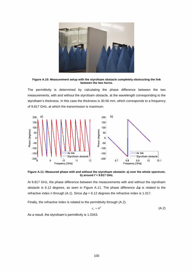
100
Figure A.10: Measurement setup with the styrofoam obstacle completely obstructing the link between the two horns.
The permittivity is determined by calculating the phase difference between the two
measurements, with and without the styrofoam obstacle, at the wavelength corresponding to the
styrofoam’s thickness. In this case the thickness is 30.56 mm, which corresponds to a frequency
of 9.817 GHz, at which the transmission is maximum.
Figure A.11: Measured phase with and without the styrofoam obstacle: a) over the whole spectrum; b) around f = 9.817 GHz.
At 9.817 GHz, the phase difference between the measurements with and without the styrofoam
obstacle is 6.12 degrees, as seen in Figure A.11. The phase difference Δφ is related to the
refractive index n through (A.1). Since Δφ = 6.12 degrees the refractive index is 1.017.
Finally, the refractive index is related to the permittivity through (A.2).
2
r n (A.2)
As a result, the styrofoam’s permittivity is 1.0343.
a) b)
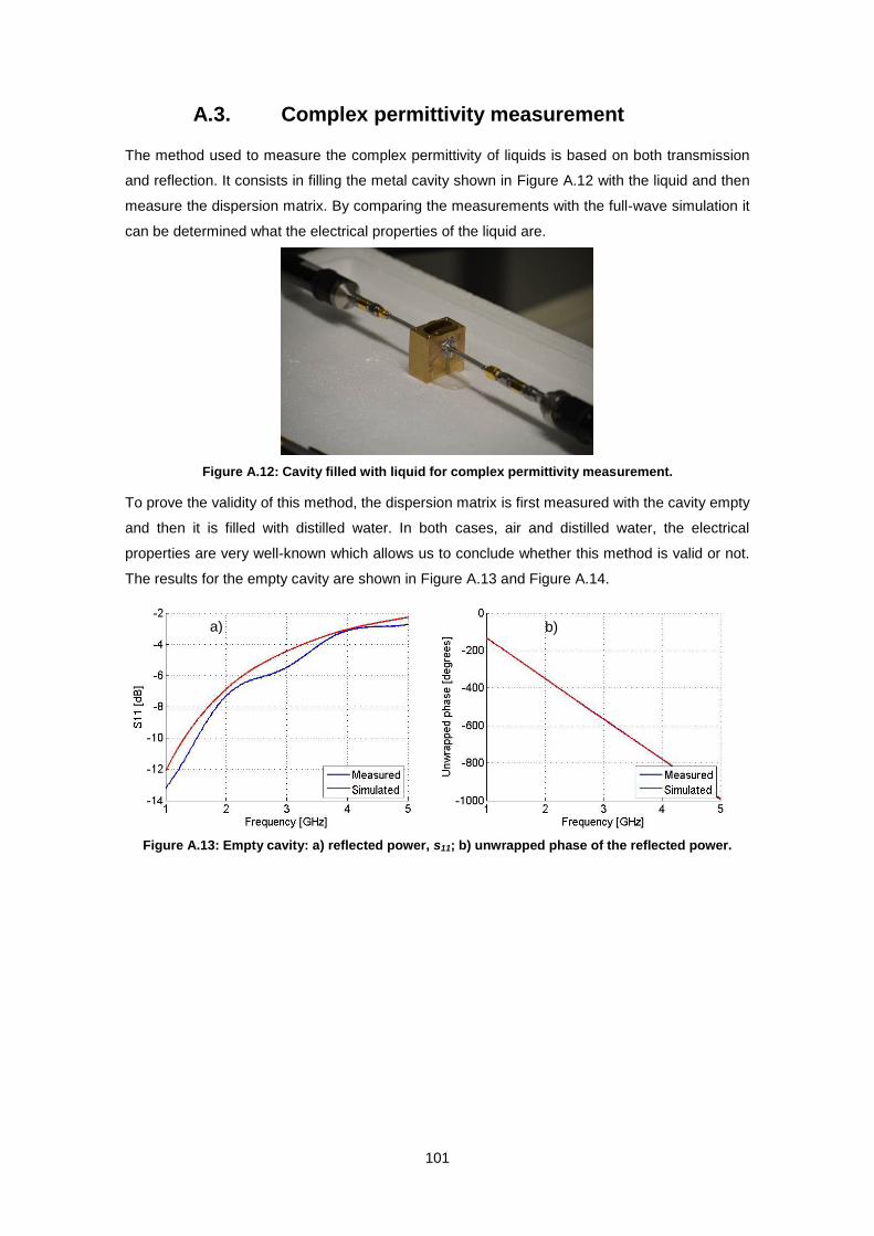
101
A.3. Complex permittivity measurement
The method used to measure the complex permittivity of liquids is based on both transmission
and reflection. It consists in filling the metal cavity shown in Figure A.12 with the liquid and then
measure the dispersion matrix. By comparing the measurements with the full-wave simulation it
can be determined what the electrical properties of the liquid are.
Figure A.12: Cavity filled with liquid for complex permittivity measurement.
To prove the validity of this method, the dispersion matrix is first measured with the cavity empty
and then it is filled with distilled water. In both cases, air and distilled water, the electrical
properties are very well-known which allows us to conclude whether this method is valid or not.
The results for the empty cavity are shown in Figure A.13 and Figure A.14.
Figure A.13: Empty cavity: a) reflected power, s11; b) unwrapped phase of the reflected power.
a) b)
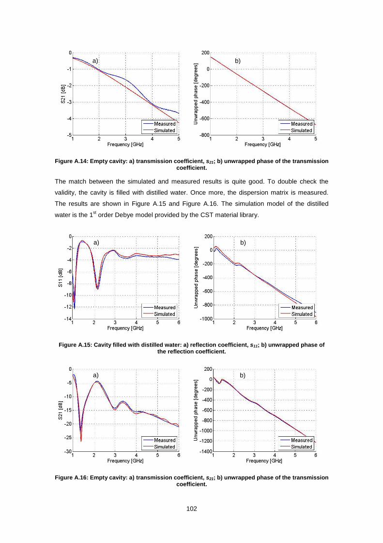
102
Figure A.14: Empty cavity: a) transmission coefficient, s21; b) unwrapped phase of the transmission coefficient.
The match between the simulated and measured results is quite good. To double check the
validity, the cavity is filled with distilled water. Once more, the dispersion matrix is measured.
The results are shown in Figure A.15 and Figure A.16. The simulation model of the distilled
water is the 1st order Debye model provided by the CST material library.
Figure A.15: Cavity filled with distilled water: a) reflection coefficient, s11; b) unwrapped phase of the reflection coefficient.
Figure A.16: Empty cavity: a) transmission coefficient, s21; b) unwrapped phase of the transmission coefficient.
a) b)
a) b)
a) b)

103
In general, the measurements are consistent with the simulated results. Based on this, it is
assumed that this method is accurate enough to allow us determining what the electrical
properties of the filling liquid are.


![GUSTAVO EDUARDO SILVA MACHADO · FM – Frequency ... PM – Phase Modulation ... Vetor de entrada de polarização Y[ ] [ ] Vetor de saída de polarização X [ ] Vetor de saída](https://static.fdocuments.in/doc/165x107/5fc05e4281affe3c881cc235/gustavo-eduardo-silva-machado-fm-a-frequency-pm-a-phase-modulation-vetor.jpg)


