Table of Content 1.3, 1.4: Introduction and Inverse Functions 2.1: Idea of Limits 2.2: Definition of Limits 2.3: Limit Laws2.4: Infinite Limits 2.5: Limits at Infinity 2.6: Continuity 3.1: Intro the Derivative 3.2: Rules of Differentiation 3.3: Product and Quotient Rules 3.4: Derivatives of Trig Functions 3.5: Derivatives as Rates of Change 3.6: The Chain Rule 3.7: Implicit Differentiation 3.8: Derivatives of Logs/Exp3.9: Derivatives of Inverse Trig Functions3.10: Related Rates 4.1: Maxima and Minima 4.2: What Derivatives Tell Us 4.3: Graphing Functions 4.4: Optimization Problems 4.5: Linear Approximation and Differentials 4.6: Mean Value Theorem 4.7: L’Hospital’s Rule 4.8: Newton’s Method 4.9: Anti-Derivatives 5.1: Approximating Area Under Curve5.2: Definite Integrals 5.3: Fundamental Theorem of Calculus 5.4: Working with Integrals 5.5: Substitution Rule

Introduction

I picked Ohio State University as my college and was able to research exactly what their requirements were for Calculus 1. This is what they will be learning during the course for a major in engineering or any other sciences.

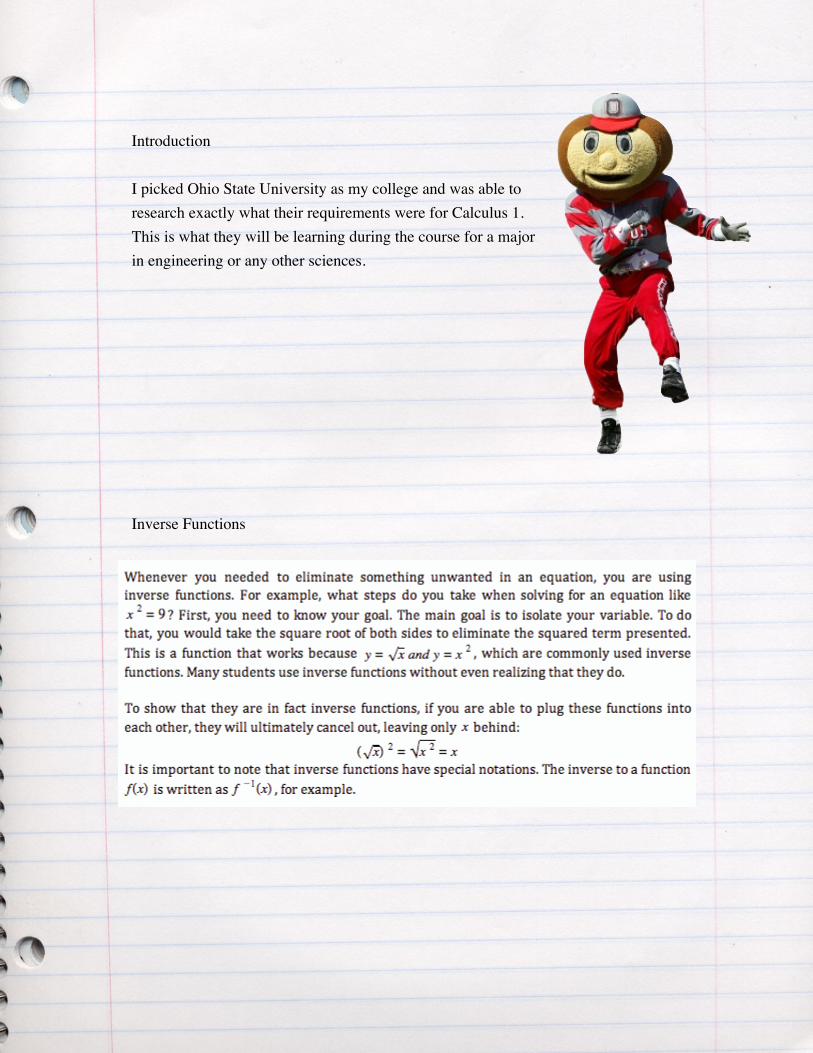
Inverse Functions

2.1: Idea of Limits

2.2: Definition of Limits

Definition 1:

The Limit Does Not Exist!

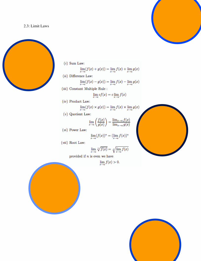
2.3: Limit Laws

2.4: Infinite Limits

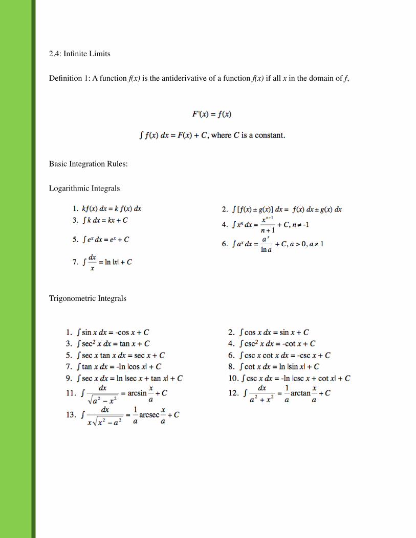
Definition 1: A function f(x) is the antiderivative of a function f(x) if all x in the domain of f,

Basic Integration Rules:

Logarithmic Integrals

Trigonometric Integrals

2.5: Limits at Infinity

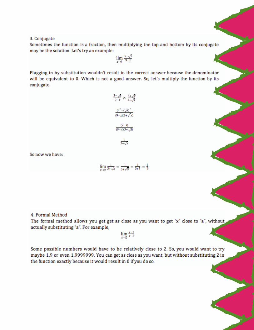
Let’s try some examples involving limits:

2.6: Continuity & Discontinuity

Example 1: Given the graph of f(x), shown below, determine if f(x) is continuous or discontinuous at x=-4, x=-2, and x=6.

Definition 1: A function is discontinuous if it does not meet one or more of the conditions of continuity. There are three specific kinds of discontinuity: jump, infinite, and removable.

3.1: Intro the Derivative

A derivative is an instantaneous rate of change at point. There are multiple rules and methods for approaches on evaluating limits.

Later to come: After this section, we will also be reviewing more about integrals. There are two different types of integrals; bound and unbound integrals. When you have bounded integrals, you are able to find the exact area between or under curves. However, when you have unbounded integrals, you can only find functions for the area between or under curves. When you have the new functions, they will always result with a c towards the end of the function for any constants.

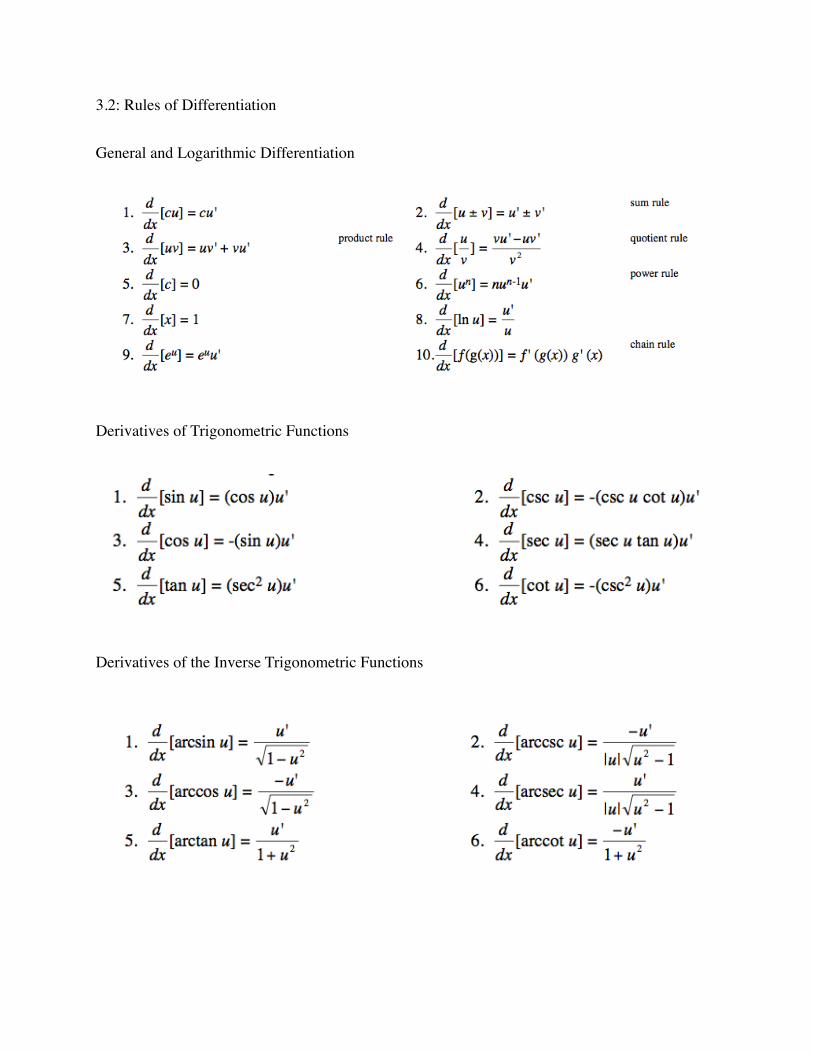
3.2: Rules of Differentiation

General and Logarithmic Differentiation

Derivatives of Trigonometric Functions

Derivatives of the Inverse Trigonometric Functions

3.3: Product and Quotient Rules

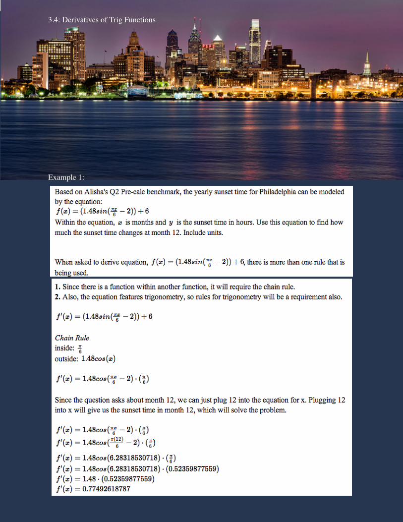
3.4: Derivatives of Trig Functions

Example 1:

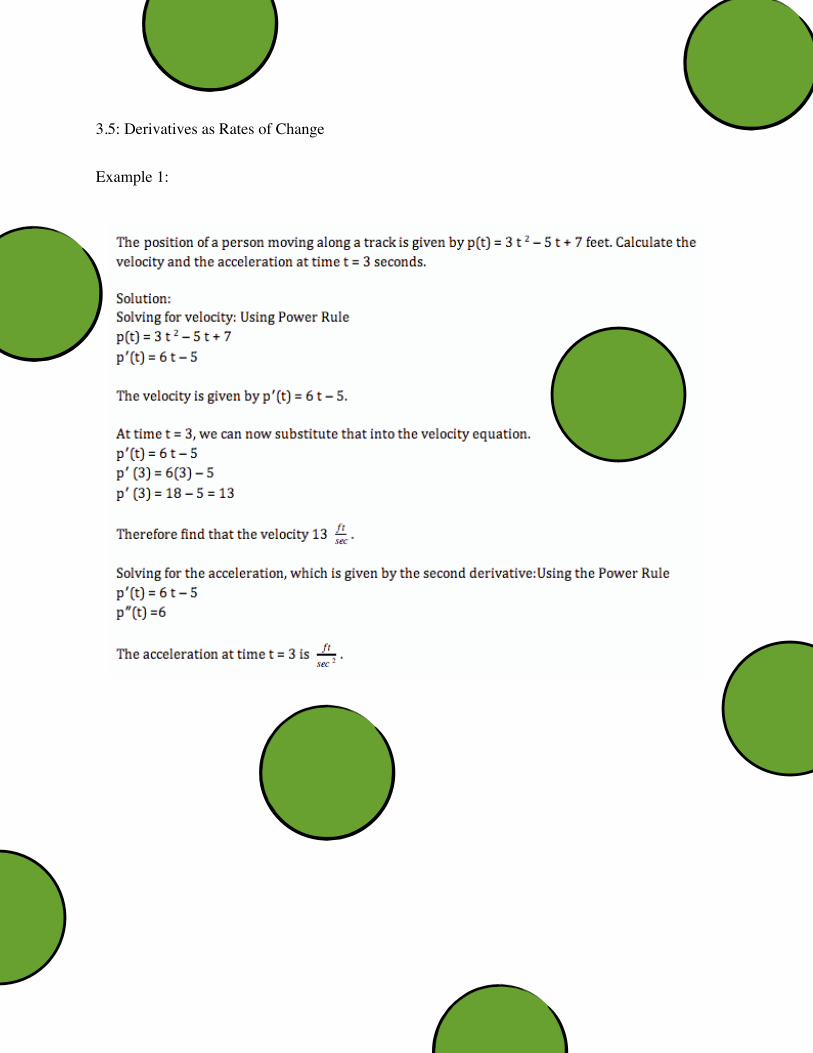
3.5: Derivatives as Rates of Change

Example 1:

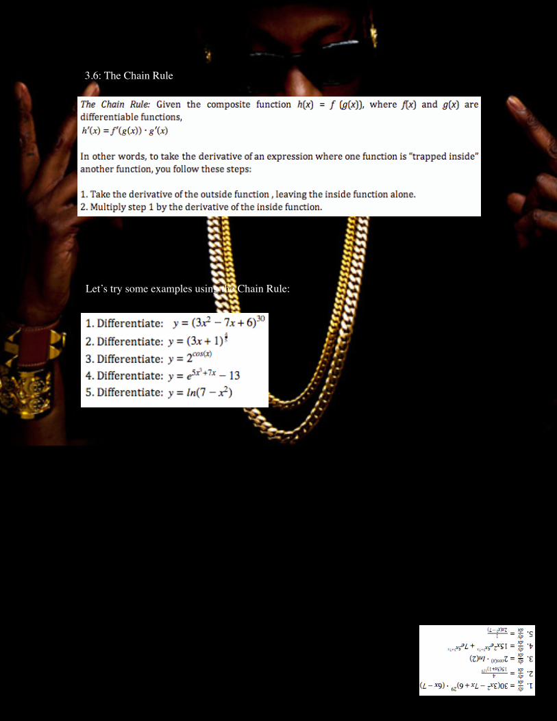
3.6: The Chain Rule

Let’s try some examples using the Chain Rule:

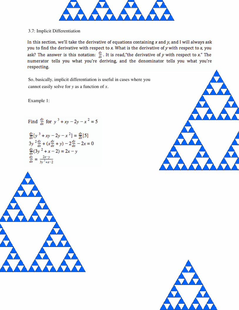
3.7: Implicit Differentiation

So, basically, implicit differentiation is useful in cases where you cannot easily solve for y as a function of x.

Example 1:

3.8: Derivatives of Logs/Exponential Functions

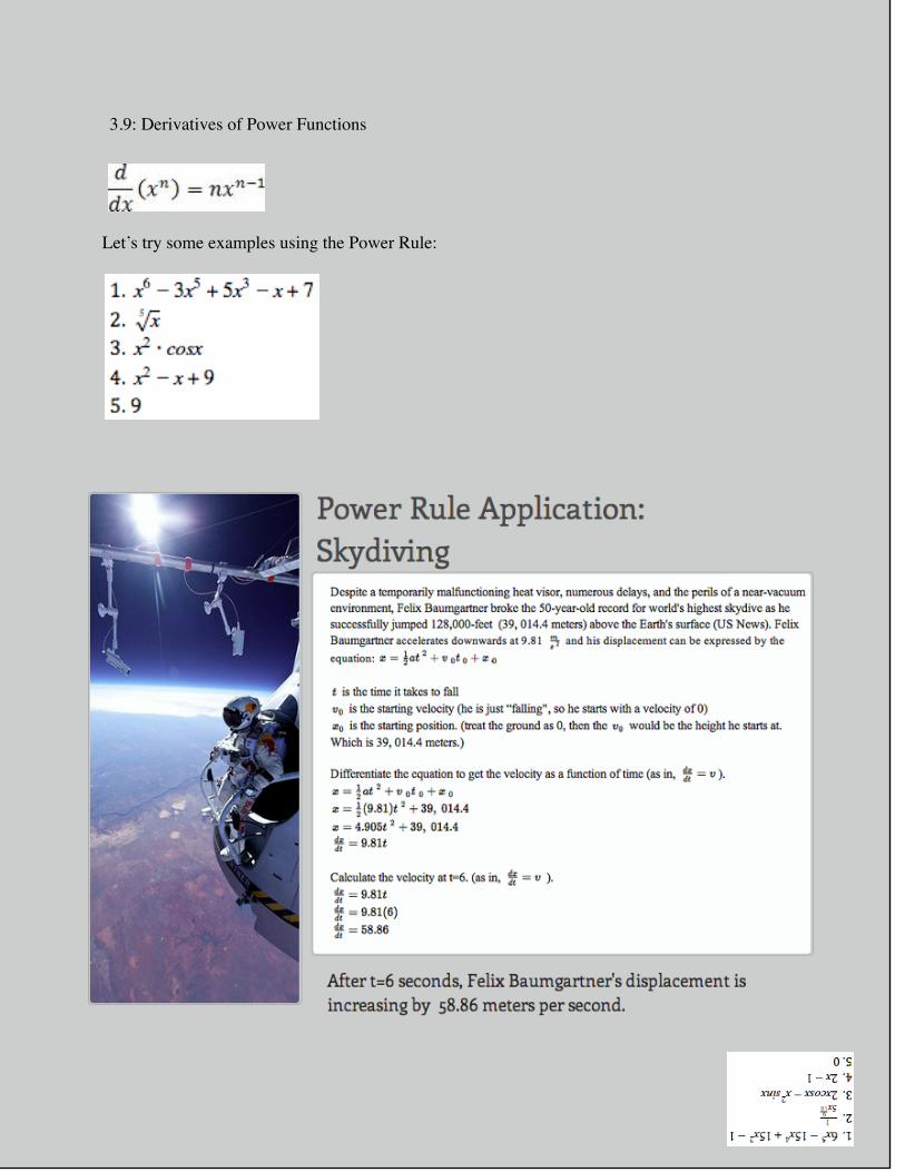
3.9: Derivatives of Power Functions

Let’s try some examples using the Power Rule:

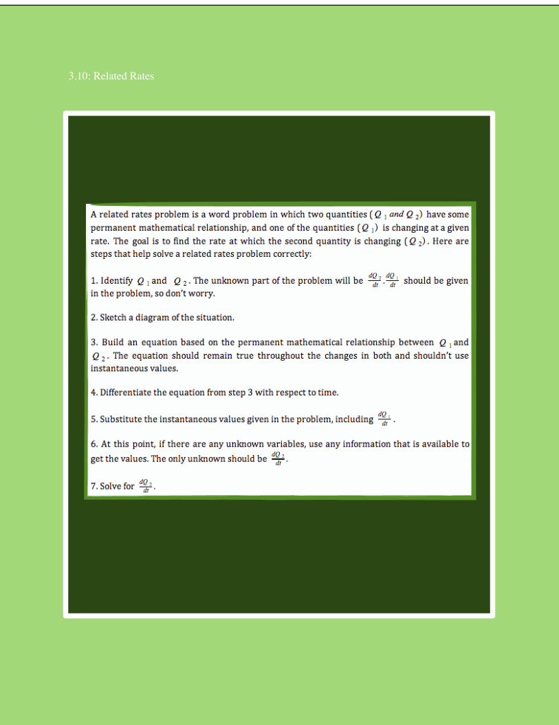
3.10: Related Rates

4.1: Maxima and Minima

Suppose f is defined on an interval and has a local maximum or minimum at the point x=a, which is not an endpoint on the interval. If f is differentiable at x=a, then f’(a)=0. This means, if a function has a local maximum or minimum that is not an endpoint on an interval, then the derivative at that point equals zero, and that pint is a critical point.

Every local maximum or minimum is a critical point, but not evert critical point is a local maximum or local minimum. At each inflection point f’’= 0, but each point where f’’= 0 is not necessarily an inflection point.

The First Derivative Test for Local Maxima and Minima Suppose p is a critical point of a continuous function f: • If f’ changes from negative to positive at p, then f has a local minimum at p. • If f’ changes from positive to negative at p, then f has a local maximum at p.

The Second Derivative Test for Local Maxima and Minima • If f’(p) = 0 and f’’(p) > 0 then f has a local minimum at p. • If f’(p) = 0 and f’’(p) < 0 then f has a local maximum at p. • If f’(p) = 0 and f’’(p) = 0 then the test says nothing.

Inflection Points and Local Maxima and Minima of the Derivative A function f with a continuous derivative has an inflection point at p if either of the following conditions hold: • f’ has a local maximum or local minimum at p. • f’’ changes signs at p.

4.2: What Derivatives Tell Us

Basically, a derivative can be looked as thought of as how much a quantity is changing at a given point. For example, the derivative of the position is instantaneous velocity. This is similar to a car’s position or distance of that car with respect to time is the instantaneous velocity. Therefore, the integral of the velocity over time is ultimately the car’s position.

In the next section, you will be informed more on what a derivative can tell you.

4.3: Graphing Functions

Derivatives can tell us a lot about a Function and its Graph• If f’ > 0 on an interval, then f(x) is increasing on that interval. • If f’ < 0 on an interval, then f(x) is decreasing on that interval.• If f’’ > 0 on an interval, then f’(x) is increasing on that interval and f(x) is concave up.• If f’’ < 0 on an interval, then f’(x) is decreasing on that interval and f(x) is concave down.

Key Terms: For the first four bullets, suppose p is a point in the domain of f. • f has a local minimum at p if f(p) is less than or equal to the values of f for points near p. • f has a local maximum at p if f(p) is greater than or equal to the values of f for points near p. • Critical Point: For any function f, a point p in the domain of f where f’(p) = 0 or f’(p) is

undefined. • Inflection Point:A point at which the graph of the function changes concavity. At the inflection

point, f’’ is either zero or undefined. • Global Maximum: The greatest value of a function f over a specifies domain. • Global Minimum: The least value of a function f over a specifies domain.

Finding the Global Maxima and Minima• Compare the values of the function at all critical points in the interval and at the end points to

find the global maximum and minimum of a continuous function on a closed interval. • Find the value of the function at all critical points and sketch or examine the graph of the

function to find the global maximum and minimum of a continuous function on an open interval.

4.4: Optimization Problems

Example 1: If you create a box by cutting squares from the corners of the piece of paper measuring 8 by 12 inches, give the dimensions of the box with the largest possible volume. (The box has no lid.)

Solution: I’ve already made a good representation of what is happening visually, now we’re ready for the math that’s involved. The volume for any box like the one presented above is V-lxwxh, where l=length, w=width, and h=height. Let’s substitute the information we know for l,w, and h.

V=(12-2x)(8-2x)xV= 4x^3-40x^2+96xThis function gives you the volume of the box hen squares of side x are cut out. So, since we want to find the value of x that makes V the largest, we an use the Extreme Value Theorem. Take the derivative with respect to xc and do a wiggle graph.

V’= 12x^2-80x+96=0 6x^2-40x+48=0

x=1.569 is the maximum volume because V’ changes from positive to negative there, meaning that V goes from increasing to decreasing.

Here are the steps for optimizing functions:

1. Construct an equation in one variable that represents what you are trying to maximize.

2. Find the derivative with respect to the variable in the problem and draw a wiggle graph.

3. Verify your solutions as the correct extrema type (either maximum or minimum) by viewing the sign changes around it in the wiggle graph.

4.5: Linear Approximation and Differentials

4.6: Mean Value Theorem

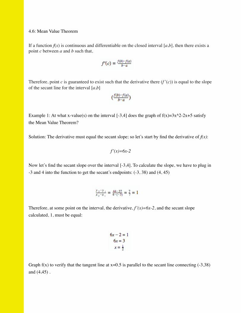
If a function f(x) is continuous and differentiable on the closed interval [a,b], then there exists a point c between a and b such that,

Therefore, point c is guaranteed to exist such that the derivative there (f ʹ′(c)) is equal to the slope of the secant line for the interval [a,b]

Example 1: At what x-value(s) on the interval [-3,4] does the graph of f(x)=3x^2-2x+5 satisfy the Mean Value Theorem?

Solution: The derivative must equal the secant slope; so let’s start by find the derivative of f(x):

f’(x)=6x-2

Now let’s find the secant slope over the interval [-3,4]. To calculate the slope, we have to plug in -3 and 4 into the function to get the secant’s endpoints: (-3, 38) and (4, 45)

Therefore, at some point on the interval, the derivative, f’(x)=6x-2, and the secant slope calculated, 1, must be equal:

Graph f(x) to verify that the tangent line at x=0.5 is parallel to the secant line connecting (-3,38) and (4,45) .

4.7: L’Hospital’s Rule

L’Hopital’s Rule states that you can take the derivative of both f(x) and g(x), and evaluate the limit using direct substitution, giving this rule:

L’Hopital’s Rule is very exclusive because it can only be used if there is an indeterminate limit in the forms of:

Example 1:

4.8: Newton’s Method Newton’s method is a method for approximating solutions to equations. 

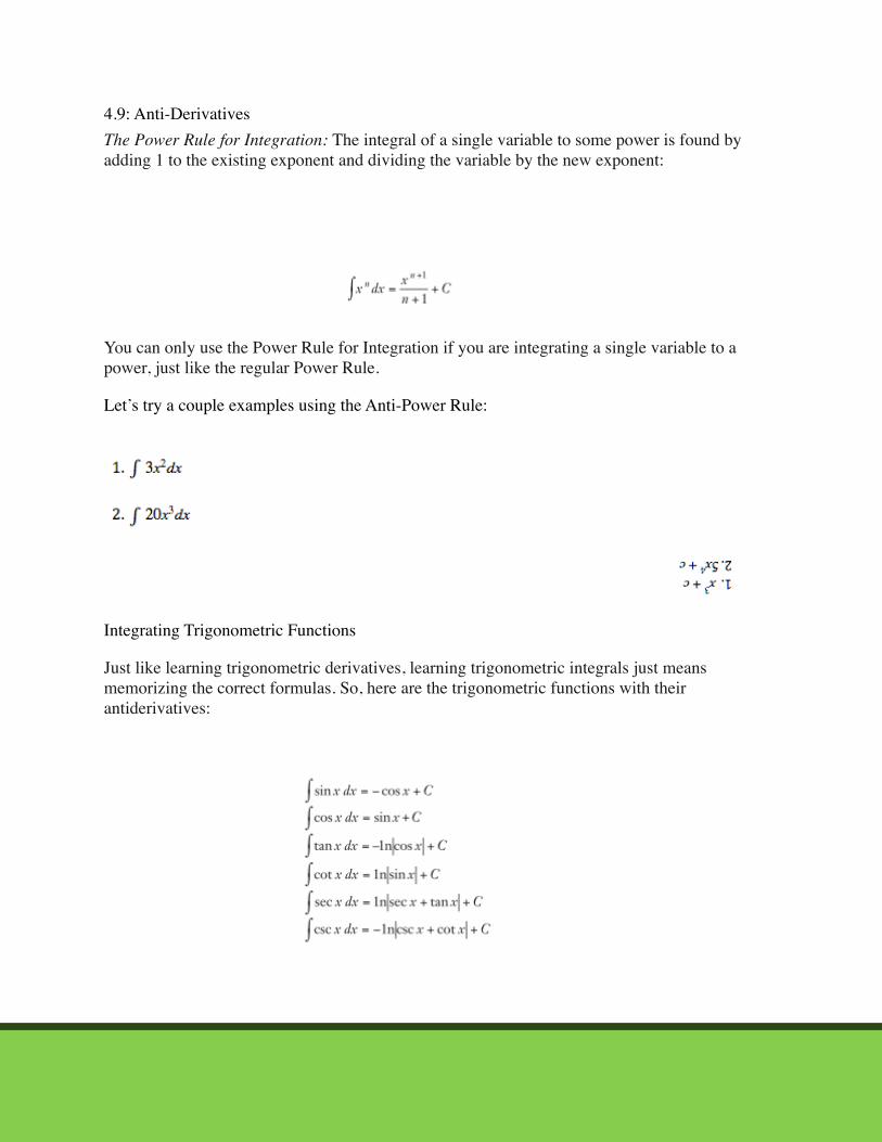
4.9: Anti-Derivatives The Power Rule for Integration: The integral of a single variable to some power is found by adding 1 to the existing exponent and dividing the variable by the new exponent:

You can only use the Power Rule for Integration if you are integrating a single variable to a power, just like the regular Power Rule.

Let’s try a couple examples using the Anti-Power Rule:

Integrating Trigonometric Functions

Just like learning trigonometric derivatives, learning trigonometric integrals just means memorizing the correct formulas. So, here are the trigonometric functions with their antiderivatives:

5.1: Approximating Area Under Curve

It is very hard to find the area under a curve, because it’s of its figure. For example, look at the graph of y=x^2+2 in the figure to the left (only the interval [0,3] is shaded in the picture).

Our goal is to try and figure out exactly how much area is represented by the shaded space. We can use past knowledge from geometry on area. But, if you may recall, there aren’t any formulas from geometry to help us find the area of a curved figure. So, strictly based on the area formulas that we do know, we’re going to approximate the area. In this section, we’re going to use the process of using rectangles to approximate area is called Riemann Sums.

Right and Left Sums

Example 1:

I’m going to approximate the shaded area under the curve using three right rectangles. Since I only have three intervals [0,3], that means each rectangle will have a width of 1. How high should each rectangle be? Since I’m using the right hand sum, the rectangles will be the height reached by the function at the right side of each interval. Look at the figure to the right.

We can approximate the area beneath the curve by adding the areas of the three rectangles together. Since the area of a rectangle is equal to its length times its width, the total area captured by the rectangles is 1x3+1x6+1x11=20. Therefore, the right Riemann approximation with n=3 rectangles is 20.

Since the intervals will no longer be even, we need to find the new width of the four rectangles. To find how wide each rectangle will be, use the formula

Midpoint Sums Calculating midpoint sums is very similar to right and left sums. However, the only difference is the heights of the rectangles. We’re going to continue to use the same example, but we’re going to just use three rectangles again to make it a bit easier (n=3).

Trapezoidal Rule

5.2: Definite Integrals

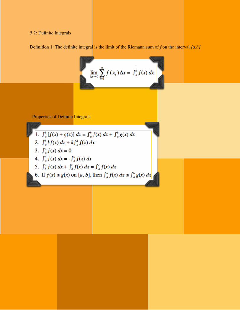
Definition 1: The definite integral is the limit of the Riemann sum of f on the interval [a,b]

Properties of Definite Integrals

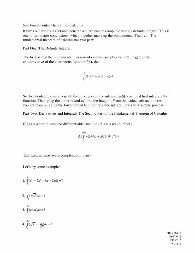
5.3: Fundamental Theorem of Calculus It turns out that the exact area beneath a curve can be computed using a definite integral. This is one of two major conclusions, which together make up the Fundamental Theorem. The fundamental theorem of calculus has two parts.

Part One: The Definite Integral

The first part of the fundamental theorem of calculus simply says that: If g(x) is the antiderivative of the continuous function f(x), then

So, to calculate the area beneath the curve f(x) on the interval [a,b], you must first integrate the function. Then, plug the upper bound (b) into the integral. From this value, subtract the result you get from plugging the lower bound (a) into the same integral. It’s a very simple process.

Part Two: Derivatives and Integrals The Second Part of the Fundamental Theorem of Calculus

If f(x) is a continuous and differentiable function (if a is a real number),

This theorem may seem complex, but it isn’t.

Let’s try some examples:

5.4: Working with Integrals

When you are working with integrals, you are then able to do a lot more things easily. For example, calculating the area between two curves. If you want to calculate the area between two continuous curves, we’ll call them f(x) and g(x), on the same x-interval [a,b], here’s what you do:

1. Set up a definite integral, with a and b as the lower and upper limits of integration, respectively.

2. You’ll rewrite it as either f(x) – g(x) or g(x) – f(x) inside the integral. To help decide which one to use, you have to graph the functions and then subtract the bottom graph from the top graph.

Graphing will become your best friend when you are working with integrals, period. When you are calculating the area between two curves, you have to make sure you are subtracting correctly. If you aren’t, you’ll result with a negative answer and you should never have a negative answer when finding the area between curves.

But, what if the graph’s are flipped? Easy, to find the shaded area, you’ll have to use two separate definite integrals. One for the interval [a,c] and one for [c,b].

5.5: Substitution Rule Using u-substitution will become second nature inside a calculus classroom. The key to u-substitution is finding a piece of the function whose derivative is also in the function. The derivative is allowed to be off by a coefficient, but ultimately must appear in the function itself.

Here are the steps you’ll follow when u-substituting:

1. Finding the u: Look for a piece of the function whose derivative is also in the function. This is most likely denominator or something being raised to a power in the function.

2. Taking the derivative: Set u equal to that piece of the function and take the derivative.

3. Simplify and Rewrite: Use your u and du expressions to replace parts of the original integral, and your new integral will be much easier to solve.

What Is Infinity?. N.d. Photograph. WonderopolisWeb. 28 May 2013. <http://wonderopolis.org/wp-content/uploads/2011/04/silver-infinity-symbol_shutterstock_64474066.jpg>.

All of the past in class worksheets given by Mr. Latimer

My 2nd Quarter Benchmark for Mr. Latimer

Veloso, Bryan. Trout Pout, A Journey: Part Three. N.d. Photograph. Word PressWeb. 28 May 2013. <http://screamingintothewind.files.wordpress.com/2012/04/lindsay-lohan2.jpg>.

N.d. Photograph. n.p. Web. 28 May 2013. <http://www1.hollins.edu/homepages/hammerpw/mathco1.gif>.

Blank Notebook Page Scan. 2006. Photograph. deviantARTWeb. 28 May 2013. <http://fc02.deviantart.net/fs9/i/2006/142/8/a/Blank_Notebook_Page_Scan_by_DragonImagine.jpg>.

Graph Paper & Graph Paper Printouts. 2013. Photograph. Keep & ShareWeb. 28 May 2013. <http://www.keepandshare.com/graphics/lp/printable/paper/graph_paper/1_8_inch_graph_paper.jpg>.

Ohio State Football Wallpaper. N.d. Photograph. BIGTENWeb. 28 May 2013. <http://bigten-online.com/wp-content/uploads/2012/08/Ohio-State-Wallpaper.jpg>.

PALAZZOLO, LARRY. How To Keep a Workout Log. 2012. Photograph. CrossFit Delaware ValleyWeb. 28 May 2013. <http://crossfitdelawarevalley.com/wp-content/uploads/2012/02/compostion-book.jpg>.

2 CHAINZ GIVING AWAY 2 CHAINS ONCE HE REACHES 1 MILLION TWITTER FOLLOWERS. 2012. Photograph. Rich Kids BrandWeb. 28 May 2013. <http://richkidsbrand.com/wp-content/uploads/2012/08/2c4.jpeg>.

Wincraft Ohio State Buckeyes Brutus Mascot Reusable Decal. 2013. Photograph. Yahoo! Web. 28 May 2013. <http://i.pgcdn.com/pi/78/34/01/783401976_160.jpg>.

Citations