STUDIES ON FILM THICKNESS AND VELOCITY DISTRIBUTION OF …
100
3Y COMMUNITY - EURATOM STUDIES ON FILM THICKNESS AND VELOCITY DISTRIBUTION ■>m weâ^Wí^ OF TWO-PHASE ANNULAR FLOW by L BIASI*, G.C. CLERICI*, R. SALA** and Α. ΤΟΖΖΓ ARS S.p.A. and «Istituto di Scienze Fisiche», University of Milan **ARS S.p.A. 1968 EURATOM/US Agreement for Cooperation EURAEC Report No. 1950 prepared by ARS S.p.A. Applicazioni e Ricerche Scientifiche, Milan - Italy Euratom Contract No. 106-66-12 TEEI
Transcript of STUDIES ON FILM THICKNESS AND VELOCITY DISTRIBUTION OF …
3Y COMMUNITY - EURATOM
STUDIES ON FILM THICKNESS AND VELOCITY DISTRIBUTION
■>m
weâ^Wí^
OF TWO-PHASE ANNULAR FLOW
by
L BIASI*, G.C. CLERICI*, R. SALA** and Α. ΤΟΖΖΓ
ARS S.p.A. and «Istituto di Scienze Fisiche», University of Milan
**ARS S.p.A.
1 9 6 8
EURATOM/US Agreement for Cooperation
EURAEC Report No. 1950 prepared by ARS S.p.A.
Applicazioni e Ricerche Scientifiche, Milan - Italy
Euratom Contract No. 106-66-12 TEEI
This document was prepared under the sponsorship of the Commission
of the European Communities in pursuance of the joint programme laid
down hy the Agreement for Cooperation signed on 8 November 1958
between the Government of the United States of America and the
European Communities.
SÌMlili It is specified that neither the Commission of the European Communities,
nor the Government of the United States, their contractors or any person
acting on their behalf :
3"* wCiAl^iríÍP!tliifi?!ww .' '^ÏIinitwlFn Make any warranty or representation, express or implied, with respect to
the accuracy; completeness, or usefulness of the information contained in
this document, or that the use of any information, apparatus, method, or
process disclosed in this document may not infringe privately owned rights
m Assume any liability with respect to the use of, or for damages resulting
from the use of any information, apparatus, method or process disclosed in
this document.
■n KHI This report is on sale at the addresses listed on cover
FB 1 2 5 . - D M 1 0 . - Lit. 1.560
When ordering, please quote the EUR number and the title, which are
indicated on the cover of each report.
¡ο2Η2$,ίβ.ΜΗ*ί&Λ KMH
Fl. 9.~
«¡»s
Printed by SMEETS Brussels, April 1968
lid ; ft-'
H^'iU 'JOSE! :l!aSuÆ
This document was reproduced on the basis of the best available copy
mM
EUR 3765 e STUDIES ON FILM THICKNESS AND VELOCITY DISTRIBUTION OF TWO-PHASE ANNULAR FLOW by L. BIASl*. G.C. CLERICI*, R. SALA** and A. TOZZI* *ARS S.p.A. and «Istituto di Scienze 1"¡siche». University of Milan **ARS S.pA. European Atomic Energy Community - EURATOM EURATOM/US Agreement for Cooperation EURAEC Report No. 1950 prepared by ARS S.p.A. Applicazioni e Ricerche Scientifiche, Milan (Italy) Euratom Contract No. 106-66-12 TEE1 Brussels, April 1967 - 94 Pages - 33 Figures - FB 125
This report contains a theoretical study on the fluidodynamics of a two-phase annular dispersed flow in adiabatic conditions. Assuming as
EUR 3765 e STUDIES ON FILM THICKNESS AND VELOCITY DISTRIBUTION OF TWO-PHASE ANNULAR FLOW by L. B1ASI*. G.C. CLERICI*, R. SALA** and A. TOZZI* *ARS S.p.A. and «Istituto di Scienze Fisiche». University of Milan **ARS S.p.A. European Atomic Energy Community - EURATOM EURATOM/US Agreement for Cooperation EURAEC Report No. 1950 prepared by ARS S.p.A. Applicazioni e Ricerche Scientifiche, Milan (Italy) Euratom Contract No. 106-66-12 TEEI Brussels, April 1967 - 94 Pages - 33 Figures - FB 125
This report contains a theoretical study on the fluidodynamics of a two-phase annular dispersed flow in adiabatic conditions. Assuming as
EUR 3765 e STUDIES ON FILM THICKNESS AND VELOCITY DISTRIBUTION OF TWO-PHASE ANNULAR FLOW by L. B1ASI*. G.C. CLERICI*. R. SALA** and A. TOZZI* *ARS S.p.A. and «Istituto di Scienze Fisiche», University of Milan **ARS S.p.A. European Atomic Energy Community - EURATOM EURATOM/US Agreement for Cooperation EURAEC Report No. 1950 prepared by ARS S.p.A. Applicazioni e Ricerche Scientifiche, Milan (Italy) Euratom Contract No. 106-66-12 TEEI Brussels, April 1967 - 94 Pages - 53 Figures - FB 125
This report contains a theoretical study on the fluidodynamics of a two-phase annular dispersed flow in adiabatic conditions. Assuming as
initial condition a situation of equilibrium, the main quantities necessary for a fully macroscopic description of the system are trie total pressure drop, the gaseous and liquid phase distribution, the velocity profiles.
Other quantities which are to be determined are the film thickness and the liquid and gas film flowrate. Τ he entrained liquid flowrate and the core gas flowrate can then be obtained from these latter by using some balance equations.
A n equation relating the liquid film thickness to the physical and geometrical parameters of the system is obtained. By solving this equation the film thickness, the liquid and gas film flowrates are calculated. 1 he results are compared with some experimental data at different conditions.
initial condition a situation of equilibrium, the main quantifies necessary for a fully macroscopic description of the system arc the total pressure drop, the gaseous and liquid phase distribution, the velocity profiles.
Other quantities which are to be determined are the film thickness and the liquid and gas film flowrate. The entrained liquid flowrate and the core gas flowrate can then be obtained from these latter by using some balance equations.
A n equation relating the liquid film thickness to the physical and geometrical parameters of the system is obtained. By solving this equation the film thickness, the liquid and gas film flowrates are calculated. The results are compared with some experimental data at different conditions.
initial condition a situation of equilibrium, the main quantities necessary for a fully macroscopic description of the system are the total pressure drop, the gaseous and liquid phase distribution, the velocity profiles.
Other quantities which are to be determined are the film thickness and the liquid and gas film flowrate. The entrained liquid flowrate and the core gas flowrate can then be obtained from these latter by using some balance equations.
A n equation relating the liquid film thickness to the physical and geometrical parameters of the system is obtained. By solving this equation the film thickness, the liquid and gas film flowrates are calculated. The results are compared with some experimental data at different conditions.
EUR 3765 e
EUROPEAN ATOMIC ENERGY COMMUNITY - EURATOM
STUDIES ON FILM THICKNESS AND VELOCITY DISTRIBUTION OF TWO-PHASE ANNULAR FLOW
by
L. BIASI*, G.C. CLERICI*, R. SALA** and A. TOZZI*
*ARS S.p.A. and «Istituto di Scienze Fisiche», University of Milan
**ARS S.p.A.
1968
EURATOM/US Agreement for Cooperation
EURAEC Report No. 1950 prepared by ARS S.p.A. Applicazioni e Ricerche Scientifiche, Milan - Italy
Euratom Contract No. 106-66-12 TEEI

SUMMARY
This report contains a theoretical study on the fluidodynamics of a two-phase annular dispersed flow in adiabatic conditions. Assuming as initial condition a situation of equilibrium, the main quantities necessary for a fully macroscopic description of the system are the total pressure drop, the gaseous and liquid phase distribution, the velocity profiles.
Other quantities which are to be determined are the film thickness and the liquid and gas film flowrate. The entrained liquid flowrate and the core gas flowrate can then be obtained from these latter by using some balance equations.
An equation relating the liquid film thickness to the physical and geometrical parameters of the system is obtained. By solving this equation the film thickness, the liquid and gas film flowrates are calculated. The results are compared with some experimental data at different conditions.
KEYWORDS
FILMS TWO-PHASE FLOW THICKNESS FLUID FLOW VELOCITY PRESSURE DISTRIBUTION DIFFERENTIAL EQUATIONS
C O N T E N T S
Introduction 5
1 - Description of the Model 7
2 - Distribution of the Liquid and
Gaseous Phase 8
3 - Film Velocity Distribution το
4 - Average Film Velocity 15
5 - Liquid and Gas Film Flovrate 17
6 - Core Velocity Distribution 19
7 - Liquid and Gas Core Flovrates 22.
8 - Film Thickness Calculation 2k
9 - Model Predictions and Comparisons 25 10 - Comparison 26
11 - Comparison with Harwell Data 58
12 - A Simplified Model g0 13 - Appendix 65
14 - Tables 67
15 - Bibliography 92

STUDIES ON FILM THICKNESS AND VELOCITY, . DISTRIBUTION OF TWO-PHASE ANNULAR FLOW U '
INTRODUCTION
This report contains a theoretical study on the fluidodynamics of a two-phase annular dispersed flow in adiabatic conditions. Assuming as initial condition a situation of equilibrium, the main quantities necessary for a fully macroscopic description of the system are the total pressure drop, the gaseous and liquid phase distribution, the velocity profiles. If the flow field is subdivided into two region "film" and "core", according to a usual representation, the other quantities which are to be determined are the film thickness and the liquid and gas film flowrate. Then the entrained liquid flowrate and the core gas flowrate can be obtained from these latter by using some balance equations. The entrainment and diffusion liquid droplet velocities are also necessary but only for the description of non equilibrium conditions. The knowledge of the equilibrium conditions here analyzed may be a useful step for this determination. An analytical solution of two-phase annular flow with liquid entrainment has been previously presented by S. Levy.—' By assuming the knowledge of the total pressure drop for unit length, Levy builds up a quantity F depending on the film thickness only. The relation between the function F and the film thickness is obtained by some plots correlating experimental measurements performed at CISE. Actually a fully analytical description of this type of flow though referred to time averaged quantities is exceedingly difficul-t. For this reason a similar approach was followed in the present vork. The basic assumption is the knowledge of the total pressure drop together with the average void fraotionO< .
Manuscript received on January 12, I968.

They are two well-studied quantities and several empirical correlations give their value «rith good accuracy. Under these t-J/o assumptions, an equation relating the liquid film thickness to the physical and geometrical parameters of the system is obtained. By solving this equation tne film thickness, the liquid and gas film flowrates are then calculated. The results are compared with some experimental data at different conditions.
1 - DESCRIPTION OF THE MODEL
The model here presented is based on a subdivision of the flow field into two regions:an annulus around the solid vails of the duct (film) and a central zone (core). Both phases are assumed to be present everywhere.The film is further subdivided into a laminar sublayer and a turbulent region. In single phase systems there exists also a buffer zone where the dynamic and eddy viscosity are comparable On the other hand in two-phase systems the mass transfer between film and core can reduce the extension of this transition regiontTherefore it can be reasonable to negxetc it when the film thickness is much smaller then the duct radius. The core is assumed to be completely turbulent. It is also stated that the motion conditions in the film are mainly affected by the physical properties of the liquid phase, whilst in the core by those of the gaseous phase. Thus, instead of establishing an actual separation of the phases, a separation is postulated in the motion conditions between the two regions. The velocity distribution in the turbulent region is obtained by using Von Karman assumption on the mixing length and taking into account the actual shear stress distribution. The integration constants are calculated by matching the velocities and their derivatives at the boundary between the laminar sublayer and the turbulent region, and at the film-core interface. Prandtl's universal velocity distribution was also tested for the core region. In both cases the value of the mixing length constant was modified as suggested by the experimental resulLS obtained at CISE. A single expression of the local void fraction of as a function of the film tiickness is introduced. A set of equations is then derived which leads to the determination of the film thickness and partial mass flow-rates.
8
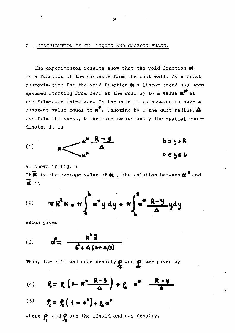
2 - DISTRIBUTION OF THE LIQUID AND GASEOUS PHASE.
The experimental results show that the void fraction 0( is a function of the distance from the duct wall. As a first approximation for the void fraction OC a linear trend has been assumed starting from zero at the wall up to a value K at the film-core interface. In the core it is assumed to have a constant value equal to K . Denoting by R the duct radius,L· the film thickness, b the core radius and y the spatial coordinate, it is
(D
as shown in fig. 1 If OC is the average value of §1 , the relation between Qf and Ot is
(2)
which gives
(3) *·= —SJL* _ b + AU+4/»)
Thus, the film and core density O and ρ are given by
(4) f- K (,. S-L·!.) t ς . . _*μ_ ( 5 )
***(<-«·)♦*«·
where O and 0 are the liquid and gas density.

Trend of DC as a function of the distance from the duct wall.
Fig. 1
IO
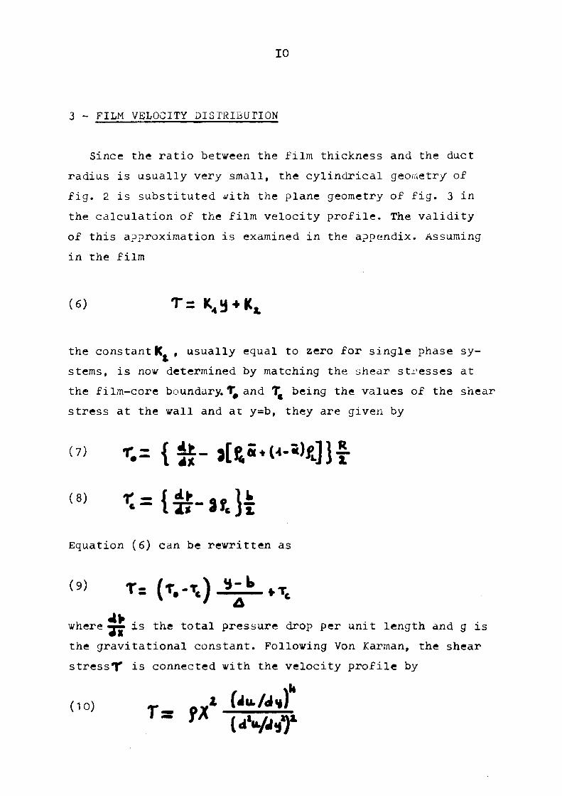
3 - FILM VELOCITY DISTRIBUTION
Since the ratio between the film thickness and the duct radius is usually very small, the cylindrical geometry of fig. 2 is substituted with the plane geometry of fig. 3 in the calculation of the film velocity profile. The validity of this approximation is examined in the appendix. Assuming in the film
(6) τ = Κ,ϊ + Ι^
the constant Κ, , usually equal to zero for single phase systems, is now determined by matching the shear stresses at the film-core boundary. Τφ and Τ being the values of the shear stress at the wall and at y=b, they are given by
(7) r-= { & - J[£5*<4-5)«.]}T
(8) r<={&-Jî.tè Equation (6) can be rewritten as
<» T= (T.-Tt)_^L,Tc
where «j— is the total pressure drop per unit length and g is the gravitational constant. Following Von Karman, the shear stressT* is connected with the velocity profile by
(10) ~ —* ÍW«U) (dV^r

II
Circular geometry of the system,
Fig. 2

12
Equivalent plane geometry.
« ν * J
■
0 b R Fig. 3
13
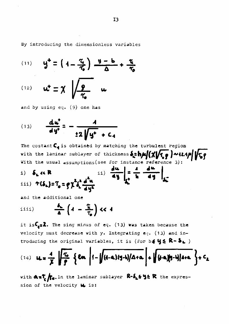
By introducing the dimensionless variables
(11)
(12) uJ » - » | f c .
and by using eq. (9) one has
(13) ά**_ 4
The costantC,· is obtained by matching the turbulent region with the laminar sublayer of thickness ¿3hiU/frlA f )A'**/1/»/l/r f With the usual assumptions(see for instance reference 3):
ui) nM-\.fÄ4j * and the additional one
κ iiii, i . (4 i ) « <
it isCs2. The sing minus of eq. (13) vas taken because the
velocity must decrease with y. Integrating eq. (13) and in
troducing the original variables, it is (for b$lj< K i^ )
(14, u.» j ff\** H-jfu^WH^*··. ♦ |((KJf)-SM** j *c
*
with A * T A"#.In the laminar sublayer Rl t$^¿R the expres
sion of the velocity ML is:
14
(15) α= Λί%-(*-ιϊ+τ(*-ι}'τΙ*'*) By e q u a t i n g eqs . (14) and (15) a t tyst-S,,,**becomes:
(16) C . s - T.i.. ~ + fë{t* * - C ^ +tiu(i-i)J± J
As it seems reasonable to think that laminar sublayer is
affected only by the liquid physical properties, whilst the
gas affects the film turbulent region through a density varia
tion, it is possible to set in eqs. (10) (I4) (15) and (16)
ßknia ¡ s ΙΙ/Ι,/ΐΑ #;fsjt.fis the average value of the film density, obtained by averaging eq. (4):
(17) tf= ?k<-«'iP*-0 R- 3/8-Δ Î R - Δ
With these substitutions the velocity profiles in the film
become:
(18)
(19)
*·Α ¿y**
f
In the above equations the only unknown quantity is the film
thickness Û (provided that the pressure drop and the average
void fraction OC are known).
15
4 AVERAGE FILM VELOCITY
The average value of the film velocity is obtained by
integrating eqs. (18) and (19) over the film flow section
(20)
= w{AA*M
f\¿ and n» can be easily calculated:
(21) Α«^(*-<--£->^
ι Λ (22) M C <{R(A .4)-4^}
rfhen A>4, introducing the nev va r i ab le ta—JËJL. A · becomes: A * *
( 2 3 )
tii-^pffti ^ψ·*** - <|* ♦ 4h
f'HIMt** -*| *
= £ ^ ~ { A*I,* Akl^ * V AM.}
j
16
Putting χ β |jf(-a.)t + * « l ^ n d Z a X + 4 , one obtains:
itfltfc lift d
I»- * tÍ3¿tf**
* fl-*) 1 3 J|^
In the case a< 1 , I and I have the same expression, whilst
I and I become: _ —
where V a 4. VM»** The separation betweeen the two cases*>i and «<l is due to the
presence of the modulus in β« . The case a=1 is a trivial one
in which V t s ^ and the solution can be obtained directly by
eq. (9)
17
5 LIQUID AND GAS FILM FLOWRATE
Neglecting the variation of the void fraction in the laminar
sublayer, the liquid filmflowrate is given by
( 2 4 )
where
( 2 5 ) A„= { RC4-4J- ¿£-**££>«*-Τ-+*"4Γ-*"^-}
(26 ) A,= M 0 A » + | - Pf- {Δ*η»»ΐί)«·«Μ(νΓ»)}
In t h e c a s e <k>4
ir*
18
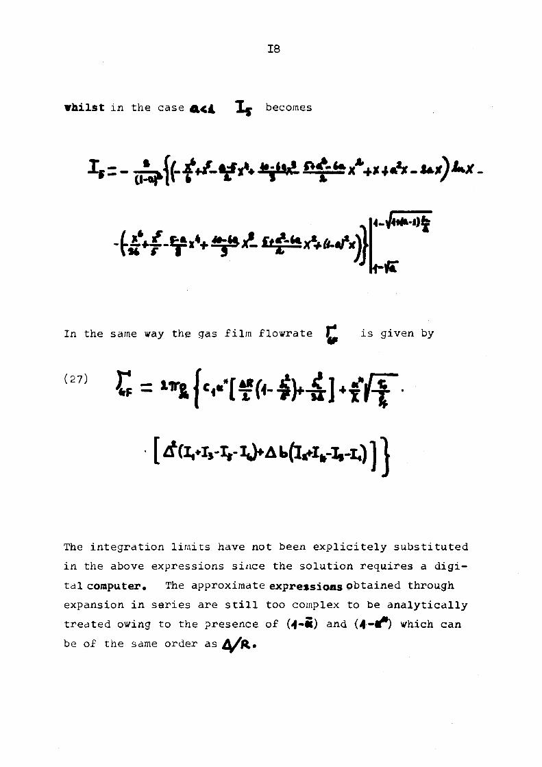
vhilst in the case A<4 I» becomes
|Λ*4-¥Λ^χΐ£^χν^]Γ
In the same way the gas film flowrate Γ* is given by
(27)
[¿f(VVVi>Al,(vvH)]]
The integration limits have not been explicitely substituted in the above expressions since the solution requires a digital computer. The approxi/nate expressions obtained through expansion in series are still too complex to be analytically treated owing to the presence of (4-fi) and (4-*) vhich can be of the same order as A/fL»
19
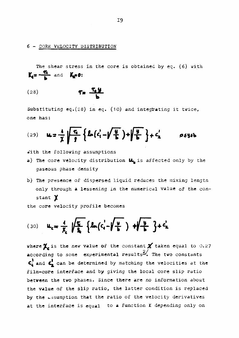
6 - CORE VELOCITY DISTRIBUTION
The shear stress in the core is obtainec by eq. (6) with K,s —ji- and K&O:
(28) f*
Substituting eq.(28) in eq. (10) and integrating it twice, one has:
(29) α=-ί^Γ{Δ.ί<;-/ϊ>Ρ}+< M|A
With the following assumptions a) The core velocity distribution U»€ is affected only by the
gaseous phase density
b) The presence of dispersed liquid reduces the mixing lengtn only through a lessening in the numerical value of the constant y.
the core velocity profile becomes
(30) ■-i^{M«:-/f)«Æ>4 where 2L is the new value of the constant jC taken equal to 0.27
2/
according to some experimental results'. The two constants
C: and C can be determined by matching the velocities at the
filmcore interface and by giving the local core slip ratio
between the two phases. Since there are no information about
the value of the slip ratio, the latter condition is replaced
by the assumption that the ratio of the velocity derivatives
at the interface is equal to a function Κ depending only on
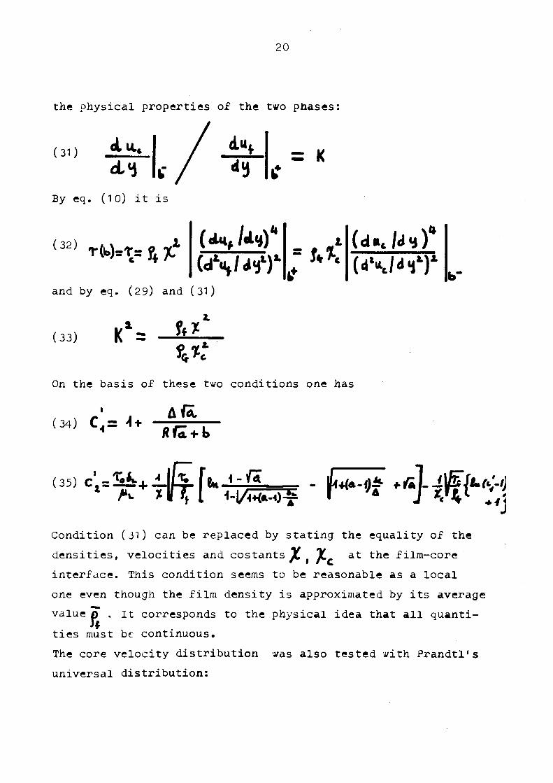
20
the physical properties of the two phases:
( 3 1 ) ¿Ht ¿Ί
A«, *3
= K
By e q . ( 10 ) i t i s
( 3 2 )
{á\ldf)í
and by e q . ( 29 ) and ( 31 )
T(W)=T= ς τα s. (d»Jd«j)' (*\W
( 3 3 ) KS ? ♦ *
t*.* On the basis of these two conditions one has
(34) C 4 = 4 + -
Rhx + b
"" <-íHlfthj&» ■ F« 4 #lt
Condition (31) can be replaced by stating the equality of the
densities, velocities and cos tants Ji JC at the filmcore
interface. This condition seems to be reasonable as a local
one even though the film density is approximated by its average
value Λ . it corresponds to the physical idea that all quanti
ties must be continuous.
The core velocity distribution was also tested with Prandtl's
universal distribution:
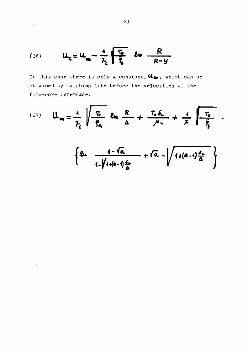
21
os) u,= α - ± € ^ u —£—
In this case there is only a constant, <¿m » which can be
obtained by matching like before the velocities at the
film-core interface.
^tít4-(37, U. Í t- * , r«J- , j
22
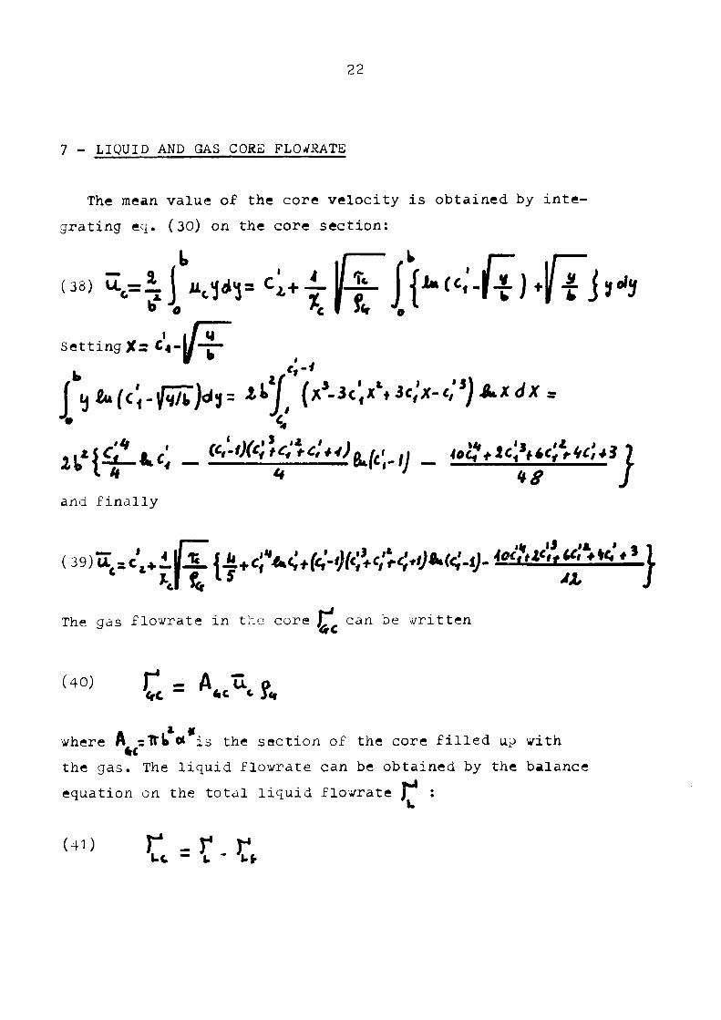
7 LIQUID AND GAS CORE FLOVRATE
The mean value of the core velocity is obtained by inte
grating eq. (30) on the core section:
ι ι A «j Setting Xr c*-\j—
(38) Ltc
and f i n a l l y
( 39,û .e .*i(Z i ¿ u ^ V t f c ' ^ w t ø ^ - ø · <«?»»% «ft*'«» ) Mi» 1 5 *t ƒ
The gas flowrate in the core Γ7 can be written
(40) y* _ Α α α
where A =1tb * is the section of the core filled up with the gas. The liquid flowrate can be obtained by the balance equation on the total liquid flowrate J :
(41) r4 - r . r Le - u ut
■23
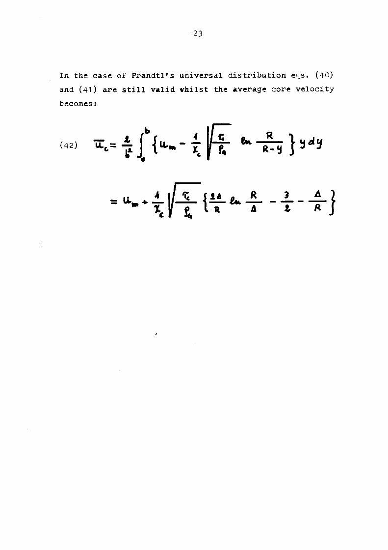
In the case of Prandtl's universal distribution eqs. (40)
and (41) are still valid whilst the average core velocity
becomes:
(42)
24
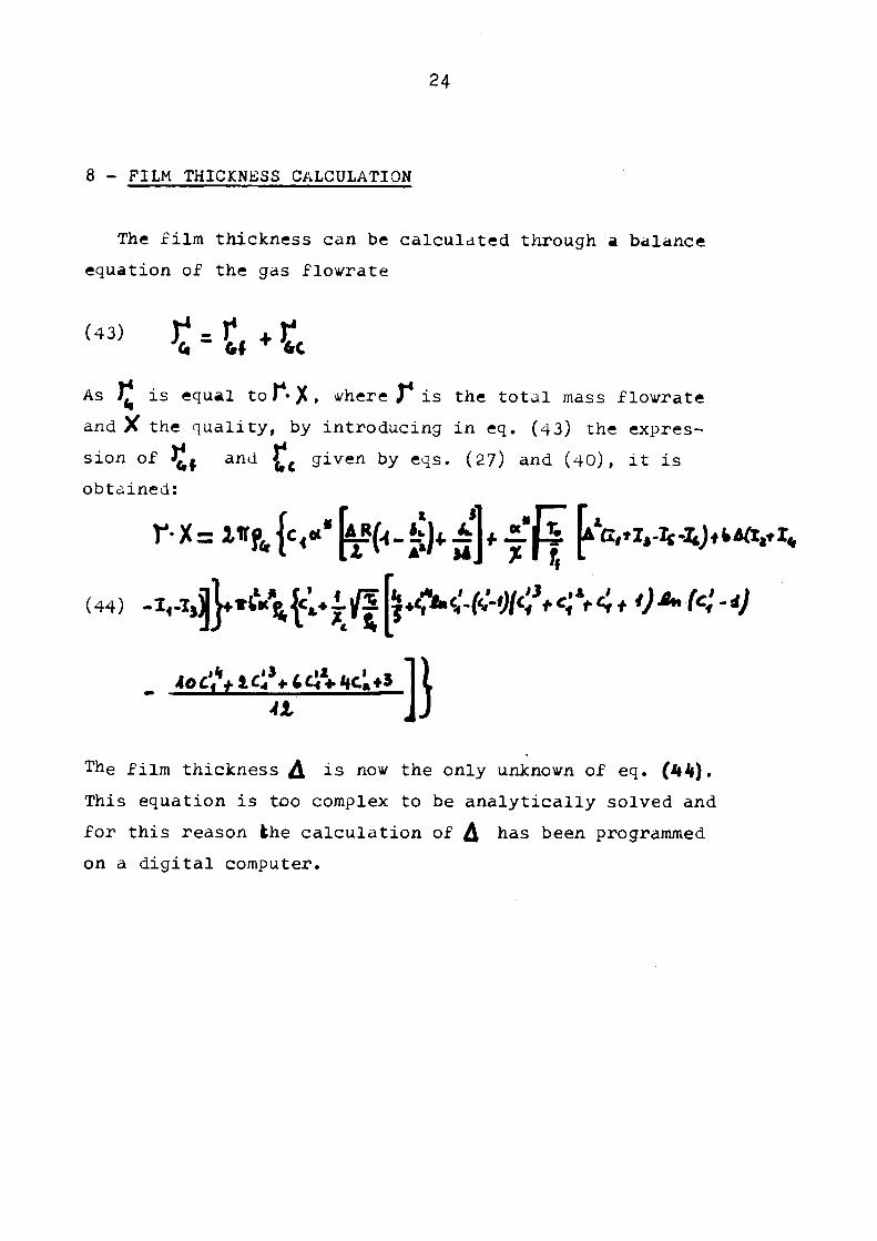
8 FILM THICKNESS CALCULATION
The film thickness can be calculated through a balance
equation of the gas flowrate
\ Gt * 6C
As j£ is equal to Γ· X, where J is the total mass flowrate
and X the quality, by introducing in eq. (43) the expres
sion of )¿f and |TC given by eqs. (27) and (40), it is
obtained:
c^icf+icA-itc^i Tí
(44)
Ao
The film thickness is now the only unknown of eq. (Mh).
This equation is too complex to be analytically solved and
for this reason the calculation of ¿^ has been programmed
on a digital computer.
25
9 - MODEL PREDICTIONS AND COMPARISON WITH EXPERIMENTAL RESULTS
The model predictions have been compared with a set of experimental results. The data taken into account are mainly related to film thickness measurements, since only a few data about jilm flowrate or entrained liquid are available at present. The comparisons have been performed for water-inert gas systems and for various values of the physical and geometrica"1 paramaters. The input data required by the computer program are:
Β = liquid surface tension Yuift = liquid and gas density /•L = liquid viscosity (9 = total specific mass flowrate X - quality R =duct radius
As previously said, the knowledge of the total pressure drop and the void fraction is also required. The program can calculate these quantities by using available correlations or read them as input data.
26
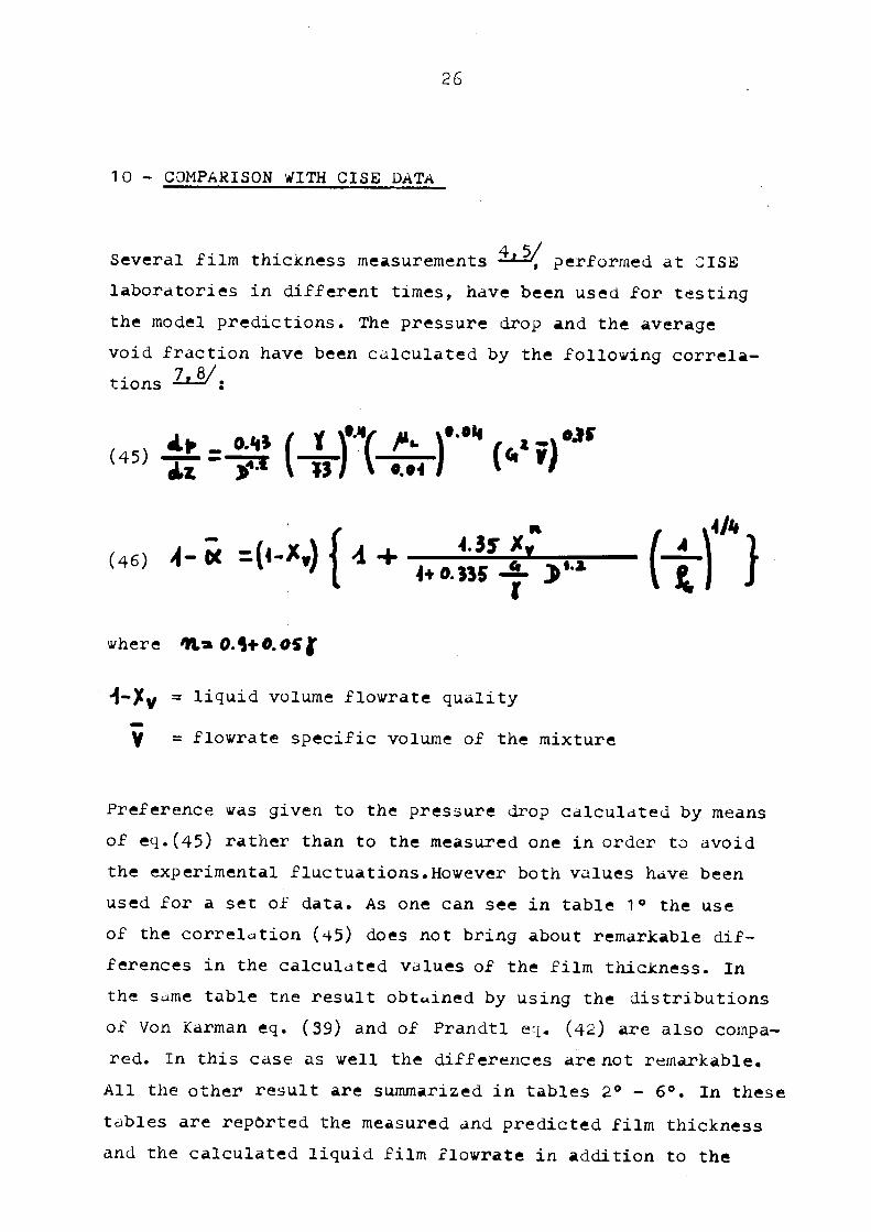
1 O - COMPARISON WITH CISE DATA
Several film thickness measurements -¿±2/ performed at CISE laboratories in different times, have been used for testing the model predictions. The pressure drop and the average void fraction have been calculated by the following correla-
7,8/ tions
(45)
where HaO.S+O.OSjf
"ί-Xy = liquid volume flowrate quality
V = flowrate specific volume of the mixture
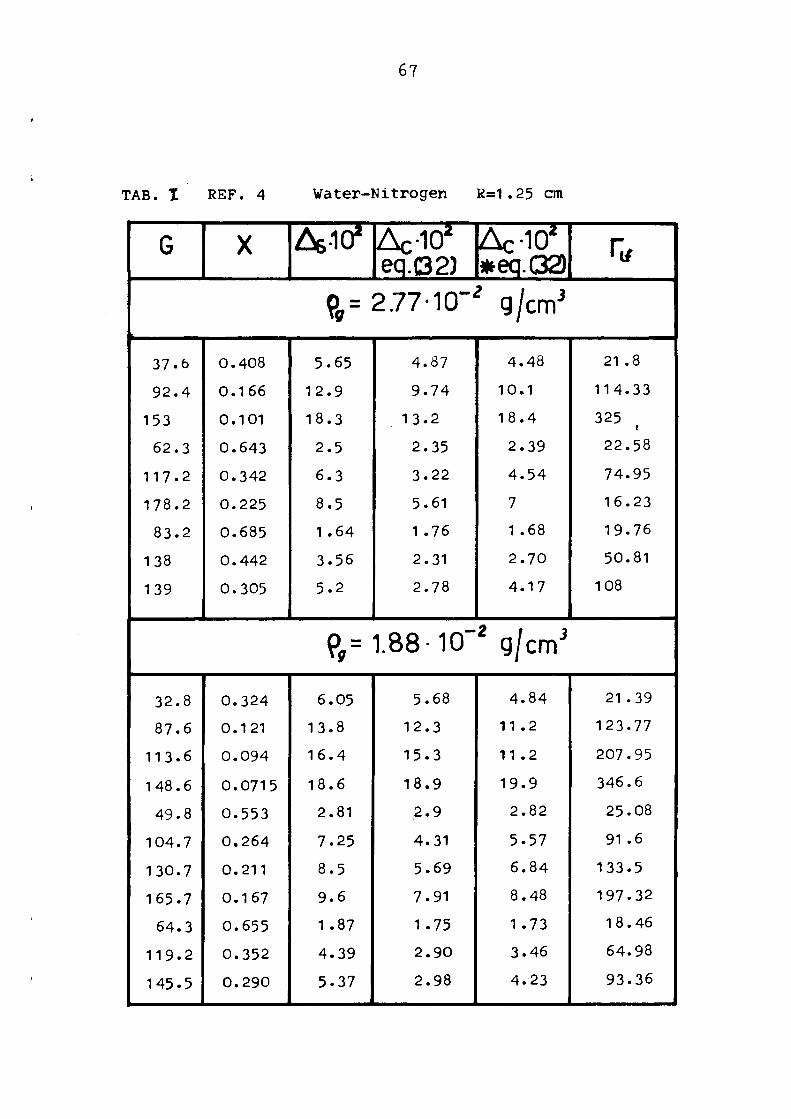
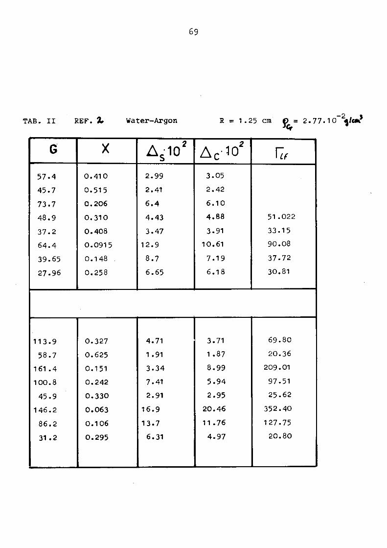
Preference was given to the pressure drop calculated by means of eq.(45) rather than to the measured one in order to avoid the experimental fluctuations.However both values have been used for a set of data. As one can see in table 1° the use of the correlation (45) does not bring about remarkable differences in the calculated values of the film thickness. In the same table the result obtained by using the distributions of Von Karman eq. (39) and of Prandtl eq- (42) are also compared. In this case as well the differences are not remarkable. All the other result are summarized in tables 2° - 6°. In these tables are reported the measured and predicted film thickness and the calculated liquid film flowrate in addition to the
27
physical paramenters describing the system. Some of the results
are also shown in figs. 4 7 31.
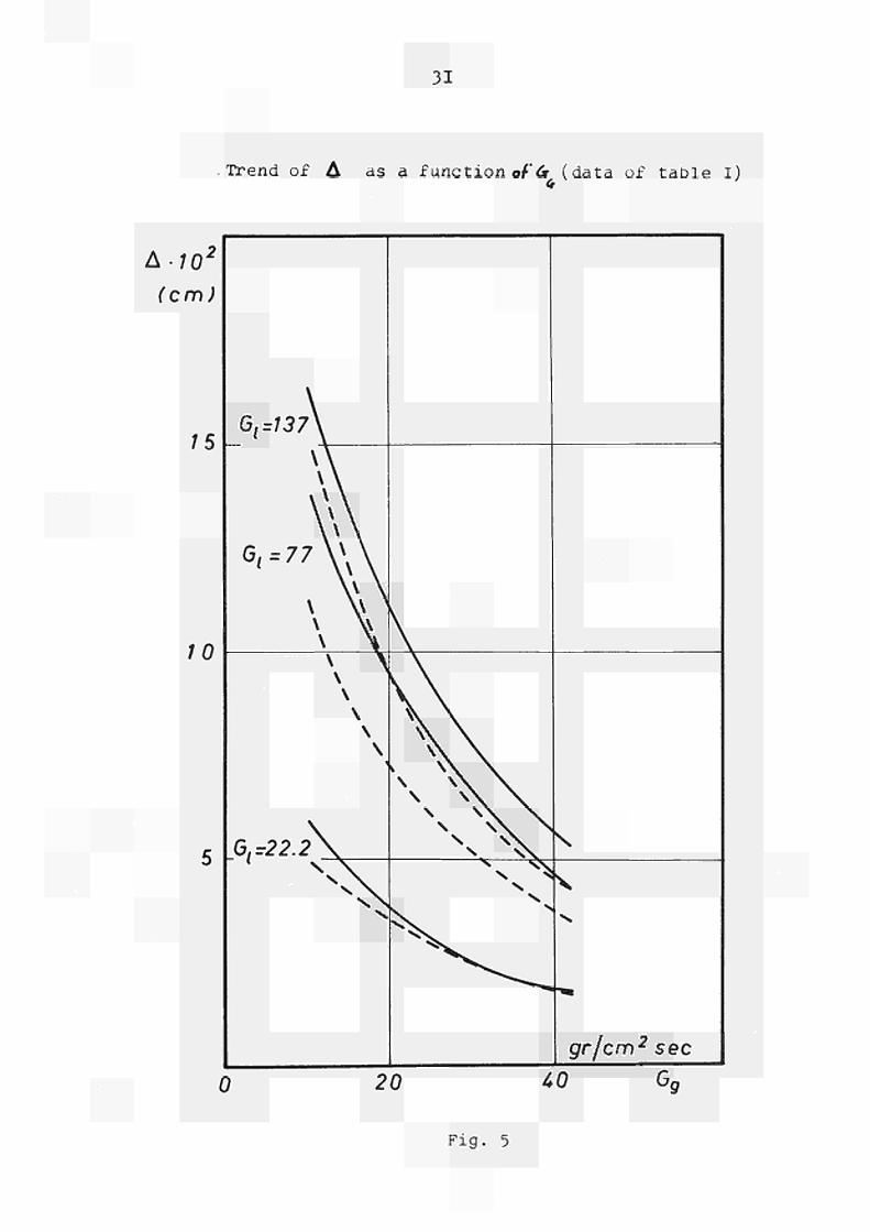
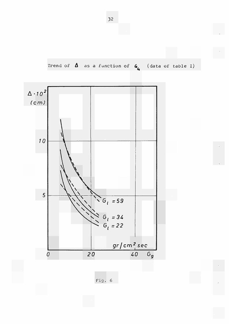
In figs. 4 76 the film thickness values of table 1° are
plotted as a function of the specific gas flowrate G^ for
some values of the specific gas flowrate Gi. . Here and in
the following figures the full line joins the experimental
points, whilst the dashed line the predicted ones.
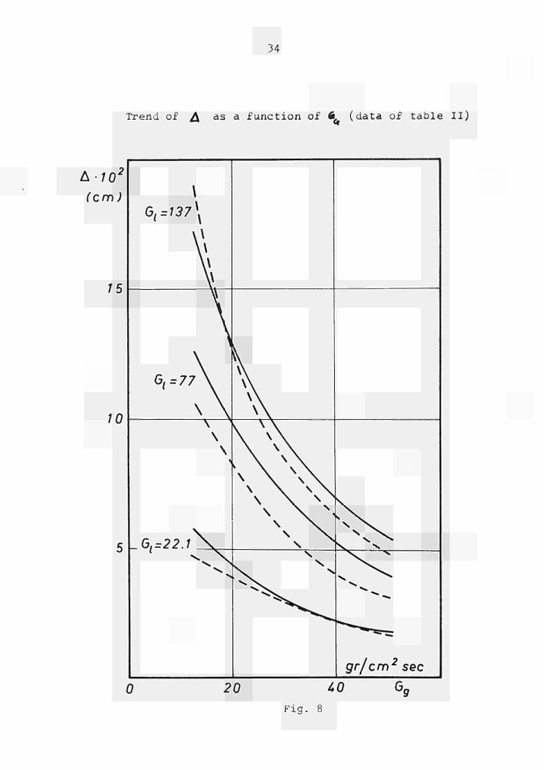
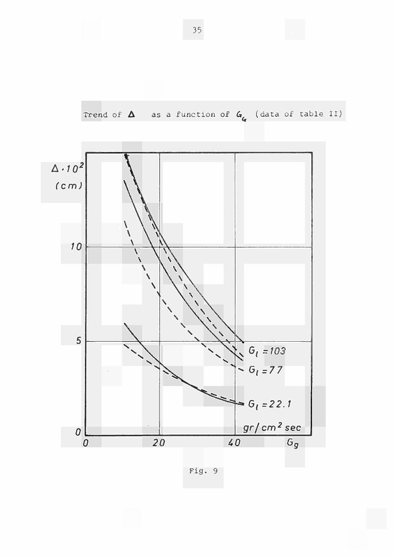
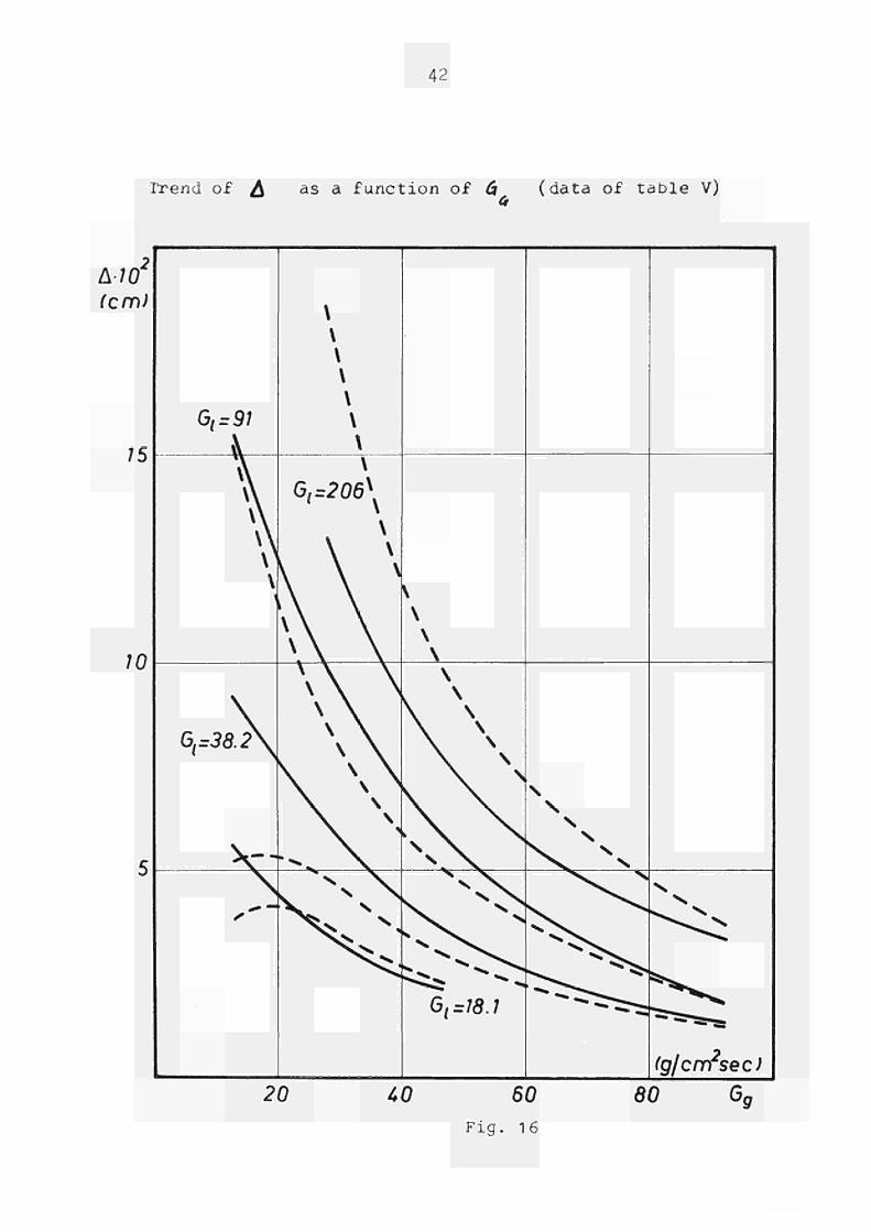
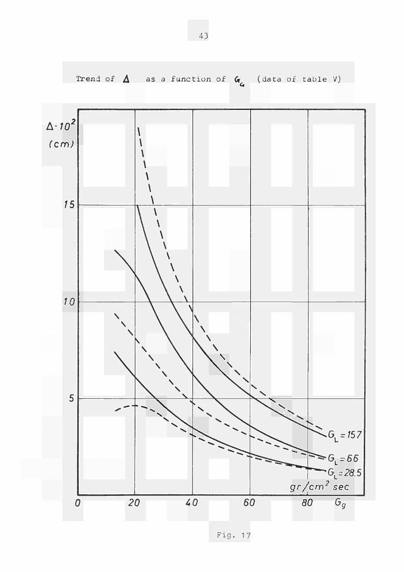
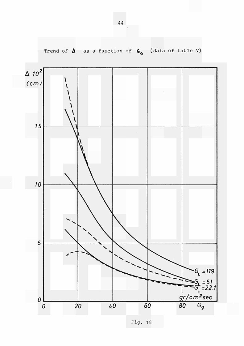
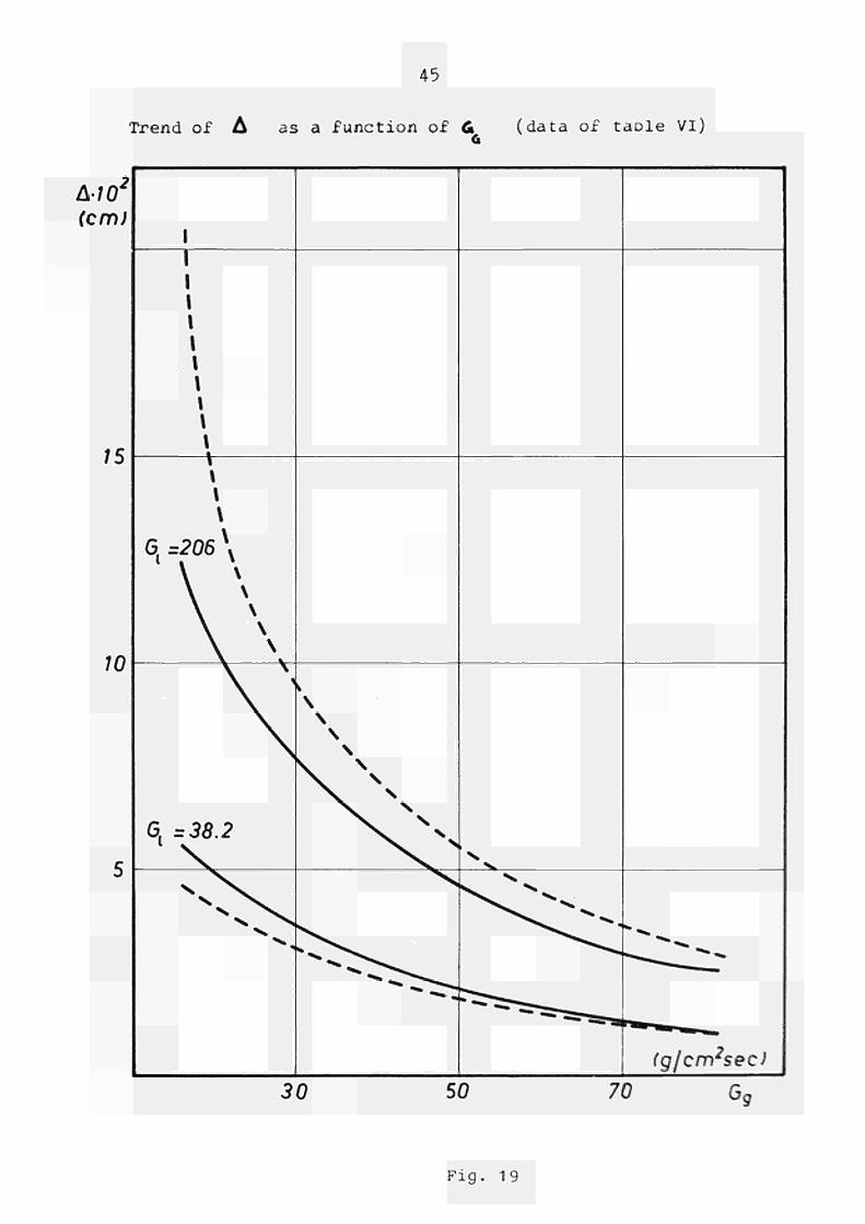
Figs. 7 7 11 show tne data of table 2°, figs. 12 # 15 those
of table 4°, figs. 16 7 18 those of table 5° and figs. 19 7 20
those of table 6°. No data of table 3° are plotted since the
experimental conditions are equal to those of table »5° which
are more recent. As one can see by the diagrams and tables the
model here presented predicts the film thickness trend as a
function of G, Χ, Ρ and R in a correct way. The agreement fails
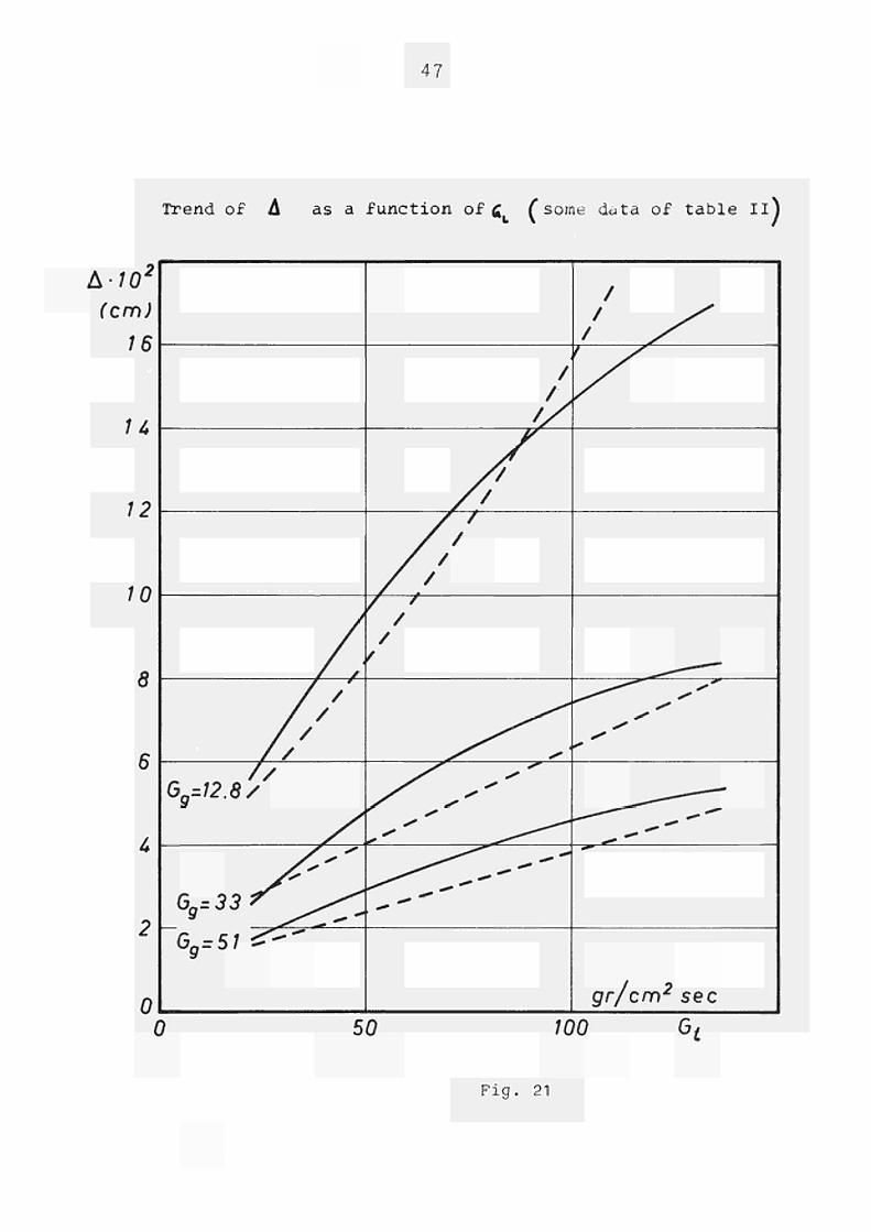
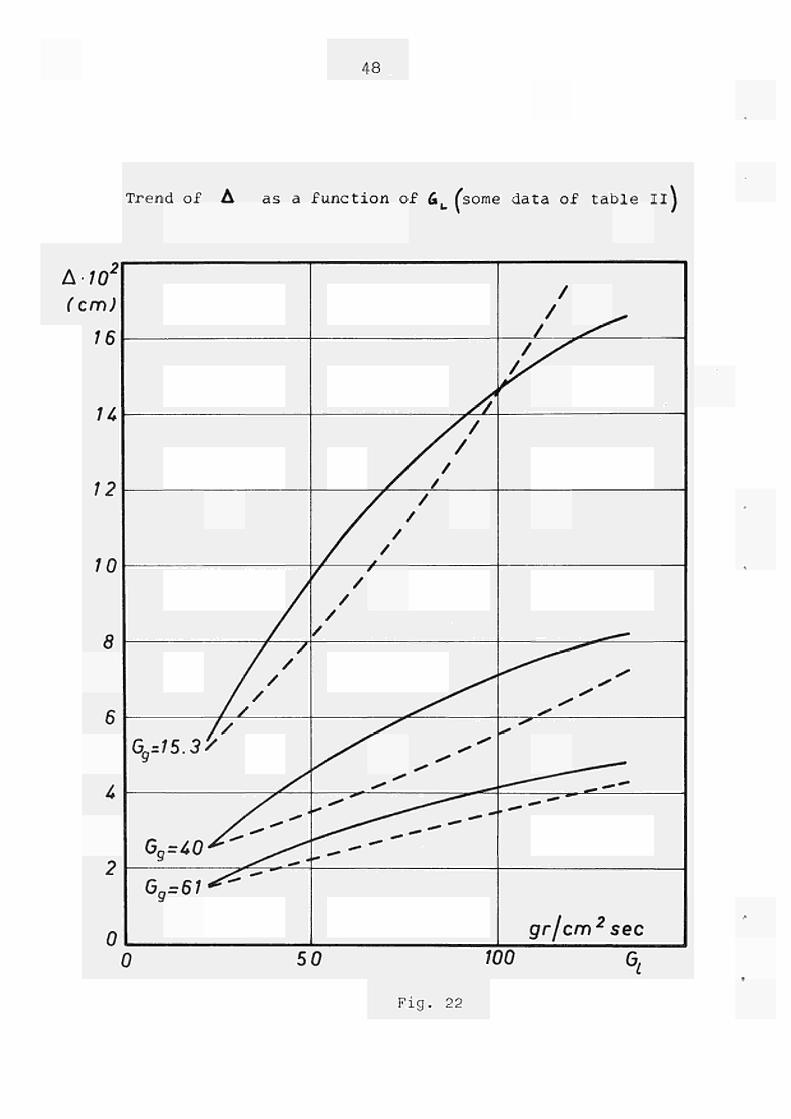
at the extreme values of X and G. This fact can be better seen
in figs. 21 22 where some data of table 2° with the film
thickness versus Qu at costoni C[ are plotted.
At very low quality the substitution of the cylindrical geome
try with the plane one and the matching of the laminar sublayer
with the turbulent region, neglecting the buffer zone, is no
longer justified. On the other hand for very high values of X
the film and laminar sublayer thickness are comparuble and
therefore the assumption _£ C á """ 1 <* {. fails.
In the range of validity of the introduced assumption, also
the quantitative agreement seems to be satisfactory. It can
be noted that the experimental measurements define an electri
cal film thickness, whilst the model predicts a thickness de
fined by purely fluidodynamics considerations.
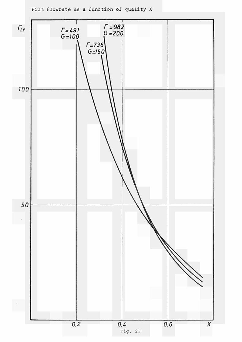
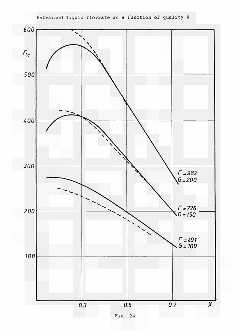
As for the liquid flowrate a test of the model predictions is
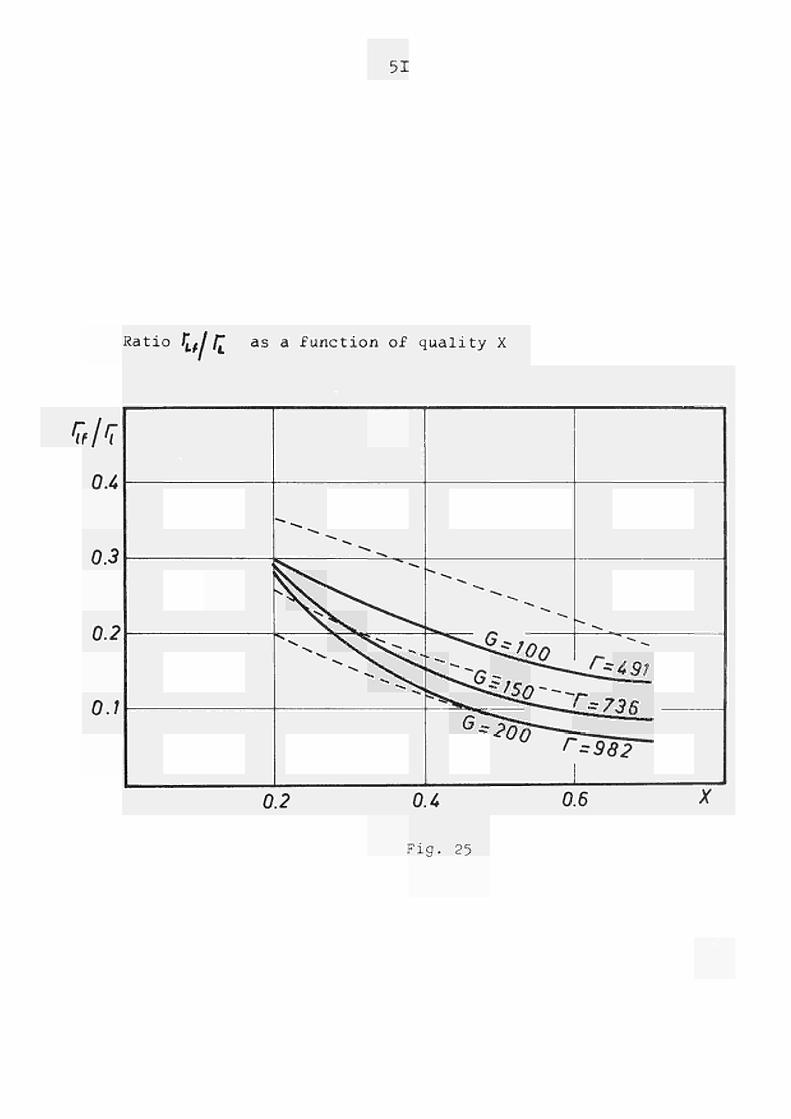
more difficult. In figs. 23 7 25 the film and entrained liquid
flowrate and the ratio F If are shown as a function ox X
28
for three values of the total flowrate (/1ri|He}34,$ft g. / it*)
The data are related to waterargon mixture at 22 ata, for a
duct with R = 1.25 cm. The trend with G and X seems to be
reasonable and under some aspects similar to one experimentally
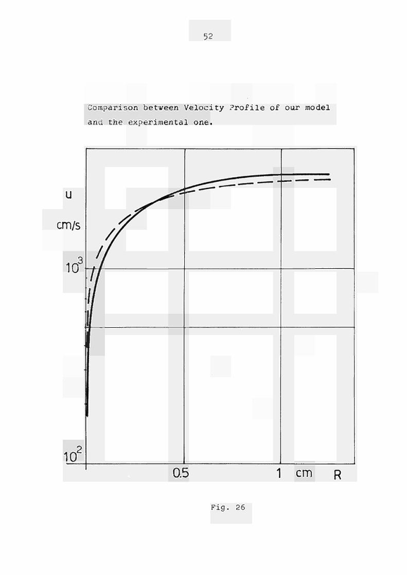
9/ observed at Harwell in steamwater system -J. Fig. (26) shr/s
the velocity profile for the case f'sîfi^/j« QX~ 0.35)
as a function of the radial coordinate. Some results reported by
Cravarolo Hassid are also shown (dashed line) in figs. (24) (25)
and (26;.
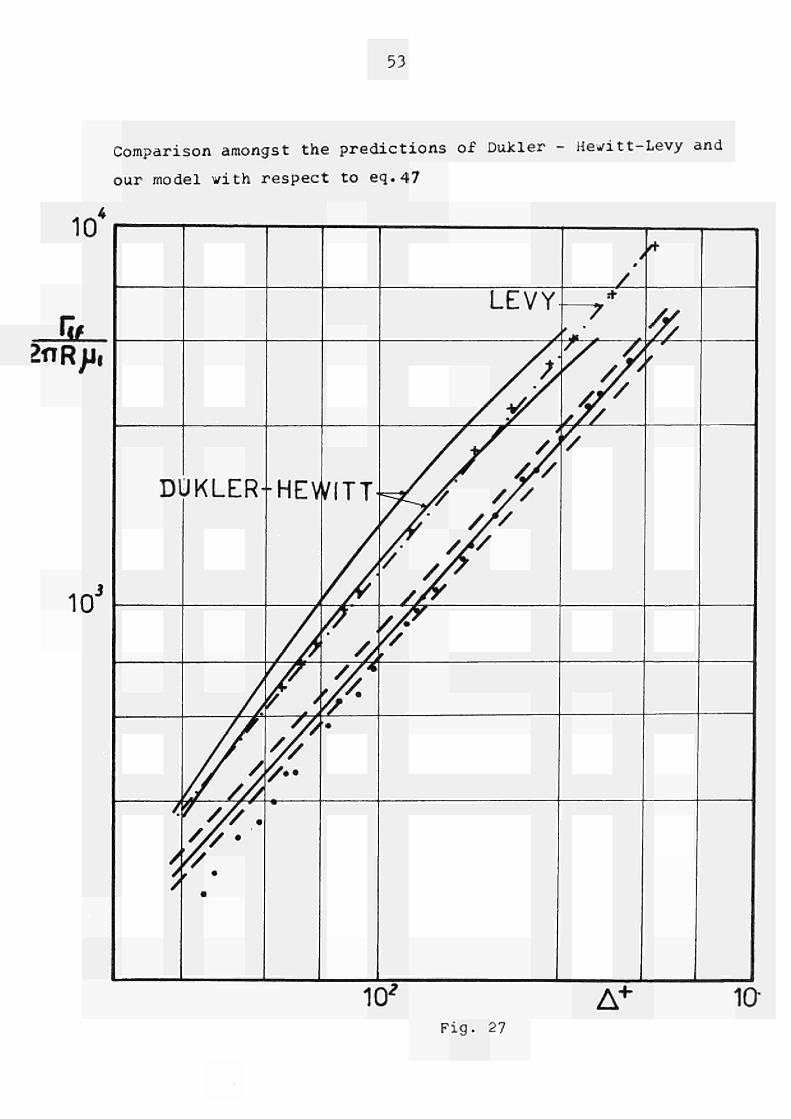
Some further comparisons have been obtained by plotting the
quantity 17 /iT^/*, versus the dimensionless thickness ¿ A S.
u In«0, · In ref.2 it is suggested that the experimental results
are well correlated by the equation
(47) _ £ f c _ = 5Λίά*)ΛΛ
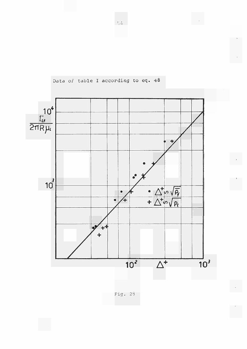
Fig . 27 is a plot, in a log log chart, of eq. (47) together i/ith the lines delimiting i 10 % variations. The dots represent the values predicted by the model for some values of table 5°. For a fully comparison the predictions of Levy Model and those of Oukler - Hewitt analysis derived from, reference 2, are also reported. AS one cea see tne values predicted by these theories are overestimated (40 - 60 y*} in comparison with tne experimental correlation. The prediction of the present model shows a very good agreement, except for the low region, where, as previously said,the hypothesis introduced are not completely satisfied. In the autnors' opinion the model predictions are best correlated by defining ¿ « A 4T Q . since γ represent the true mean
film density. Since it is always 9 < 9 » vith this definition
29
the predicted values are no longer in agreement with eq. (H7),
as shown in_fig. 28 /here some data of table 1 ° are plotted.
The relation between Γ*. /"ITJ>/*L and tne new ¿ becomes:
(48)
Figs. 29 7 31 show the data of tables 1°,2°,6° and those cor
respondin
eq. (48).
o responding to G = 100, 150, 200, gr/cm. sec vith the line of

30
Trend of Δ as a function of Ä (data of table I)
^g. 4
31
Trend of Δ as a f unction of Cr (data of table I)
Fig. 5
32
Trend of Δ as a function of 6 (data of table I)
Δ-/0 (cm)
Fig. 6

33
Trend of Δ as a function of <* (data of table II)
AIO (cm)
60 G,
34
Trend of Δ as a function of 6 (data of table II)
Fig. 8
35
Trend of Δ as a function of G, (data of table II)
A>102
(cm)
10
0
\ \ Í \ \
\ \
\ >
\
\
\
>
\ χ v, \ N» X
V
\
\ \
\ x
\
\ x
\
\ x
\ \ \ \
N \Λ\
v \ \ >
^ X \.
χ >» U
Gi =103
'** Gl=77
^Gl=22.1
gr/ cm2 sec
20 ¿0
Fig. 9
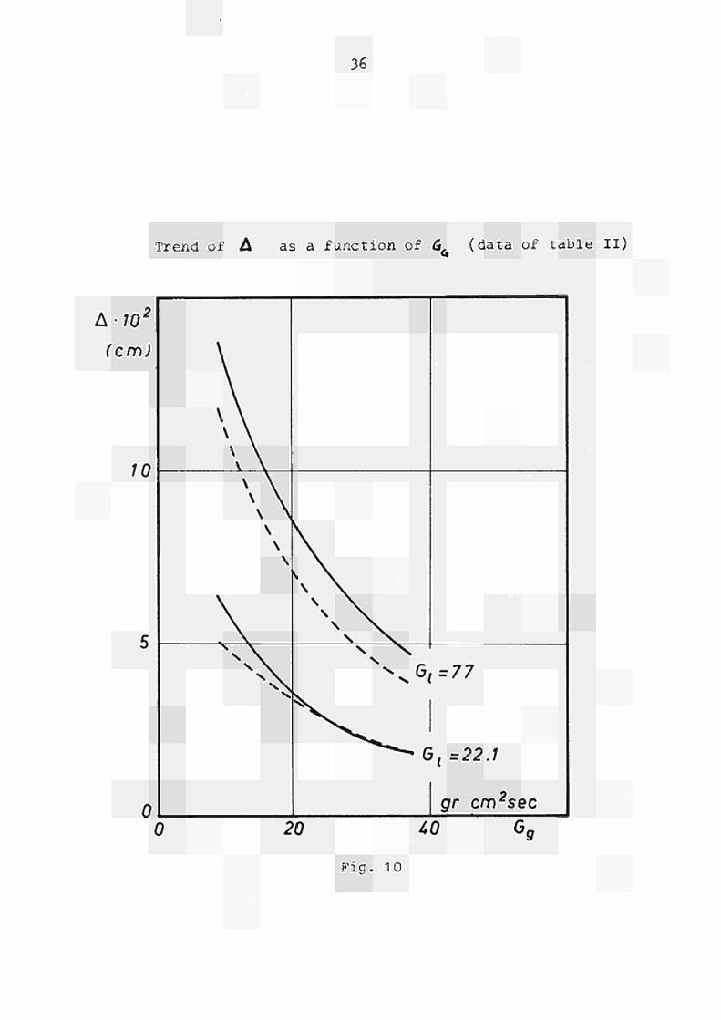
36
Trend of Δ as a function of 0, (data of table II)
Δ-70
(cm)
Fig . 10
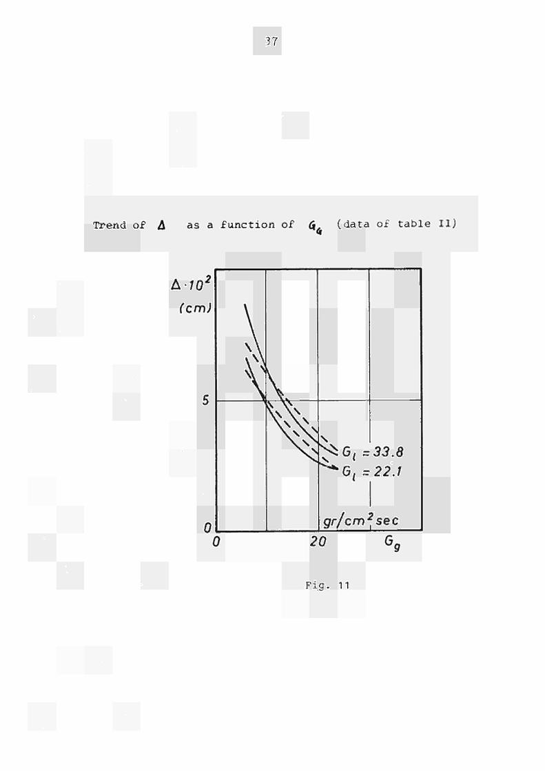
37
Trend of Δ as a function of Ú, (data of table II)
Δ-/0*
(cm)
\ \
N7\
gr/cm'
33.8
22.1
tsec
0 20
Fig. 11
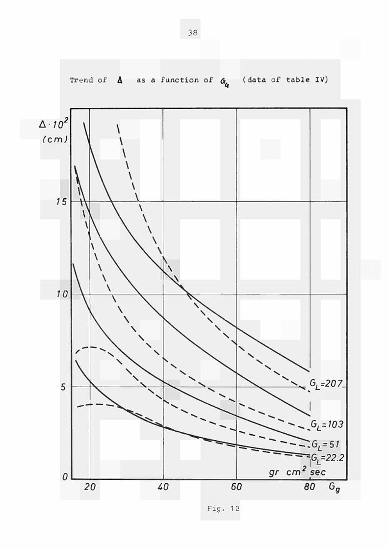
38
Trend of A as a function of Λ (data of t ab le IV) ft
\-102
(cm)
15
10
5
0
\
\ \ 0 \
s~
\
\ \ \ \ \ \ \ \ \ \
\ \ \ \ \
\ \ \
\ \ \ \ \ \ \
\ \ \ \
, \ \ \ \
\ \ \ \
^ Χ ν \ \
X x . Χ Ν X \ X. v.
^ ^ ^ . ^ ^ ^
\
\X N X .
χ \ \ \ N
\ X Χ . Ν
s \ Ν χ .
\ Χ X X , >v
^ χ ^ >* ^ ^ v. * ^ X ^ "*-"S ^ x .
Ν ^ X
\ x^ ν X, ^ X . >s
X x. χ . "X GL=207_
^ x .
""^\Λ ^ A= W3
^^Srrsr*=r*GL=22.2 gr cm2 sec
20 40 60 80 Gt
F i g . 12

39
Trend of A as a funct ion of û (data of t ab le V)
A-10
(cm)
15
10
\ \
\ \
\
\ \
\ \
\ \
\ \
\ \
\ \
\ \ \
\ V x \ \ \ \ \ \ >
\ \ \ \ \
\ \
\ \
V x
X \ N
X \ \
N
\ X \ \ X \
X >v ν χ
v. X . χ X
χ ->» χ >*
I
\
s\
Λχ
^ V X
χ \ \ Χ Ν
X χ \ ^χ
χ X^ χ χ
V ^ χ ^ ^ χ
X — V
s. \
\ χ v. \
v. — N. X .
>s. X Χ. ν
>* x^ .
gr/cm1
GL=207-
GL=103
GL=51
GL=22.2
* sec
20 40 60
Fig . 13
60 Gt

40
Trend of Δ as a funct ion of út (data of t ab le IV)
Fig . 14
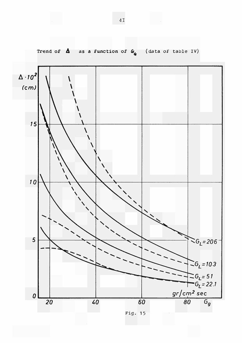
41
Trend of Δ as a funct ion of fr. (data of t ab le IV)
Δ-70*
(cm)
75
70
5
0
\
\
^ \
\ \
\ \
\ \
\ \
i \ \
"v <
__ _
\ \ X
\ \ X
\ \ \ >
\ \ \
\ \ \
\ \ \
\ \ N
\ \
\ \
ν ^ \ \ \ X
\ \ \ \
x \ . χ ν χ χ χ x χ
Ν. χ χ X
X N. _2χ
N ^ ^ . ^ f c
X N ^ V w ^
^ " » s ^ ^ ^ ^ ^
\
\
\
χ \ Χ ν ^^ > χ \
\ \
\ \
\ \
V X v Ν
^ X^ X ^ χ
X X . X \
χ χ X>^ ^
^s. X ^ ^ >* ^ X ^ " « ^ ^ ^ .
* > ^ _
^ Ä ^
χ X X
Vx
V N
•^ ^ v ^ *** ^ v ^ *»* ^ ^
^ ^ ^ ^ ^ ^ ^^
^ " " " ^ ^ ^ ^
^GL=206~
^.GL=103
^ : G L = 5 7
■*-GL3 22.7
gr/cm2 sec
20 40 60
F i g . 15
80 Gt
42
Trend of Δ as a function of Ct (data of t ab le V) ft
Δ-70
(cm)
75
70
G(=91 λ
\ \
\ \
\ \
\ \
\>
\
<
Gl=38.Z\
Φ* —
s
\
\
\
\
\
\
\
\
G(=206\
\
\ \
V \ \
A \ \ \ \
\ \ \
\ \ \
\ \
\ \
\ \
V \ \ \ \
λ
\ \ \ \
χ ^
* *** X χ χ
ν N
X Χ. ν X
N X X
\
\
\
\
\
v \
\ \ \ \
\ \ χ \
k χ, x^ \ X
N X >. χ
ν X V ^ X
X x Χ . N
* χ
^ ^ :
G(=18.1
\ X
s s
X. s χ V Χ . ν
χ χ ^ < χ ^
^^ — ^ ^ fc .
Ν. « ^ «S, ^ ■ χ , ^ ^
^ ν ^
(g/cm2sec)
20 40 60 80 G,
F i g . 16
43
Trend of Λ as a function of 0, (data of table V)
Δ70'
(cm)
15
10
\
\
\
*+■ ■*"
\
\
\
\
\
\
\
\ \
\ \
\ \
\ \
\ \
\ \
\ \ \
\ \ \
\ \ \
\ \ \
\ \
\ \
\ \
\ \
\ \ χ \
χ ν χ^ >
*"*x X». ν X
v. X N. χ
v.
\
\
\ \
\ \ \ \
. X \
ν» X s χ^
ν χ
^ X ^
\ X
χ X χ \
■
^ G L , 7 5 7
^ G L ^ 6 6
"GLr2ô.5
'cm2 sec
0 20 40 60 80 G,
Fig. 17
44
Trend of Δ as a function of G (data of t ab l e V)
Δ -70' (cm)
75
70
0
\ \
\
\
\
\ \
\ \
*«» V
rf" "~ /
\
s \ \ χ
\ χ χ Ν
X v. —Χ Ν ^ ^ ^ V X N. \
«V X s
^--Ox^ GL=77S ^ 6 , = 5 7 ^^ Gl =2 2.1
gr/cm2sec 20 40 60 80 G,
Fig . 18
45
Trend of Δ as a function of 6 (data of taDle VI)
Δ-70' (cm)
75
70
\ \ \ \ \ \ \
G( =206 \ \ \ \ \ \ \ \ \ \ \
\ \
Gt =38.2
Χ, X . χ χ N, x^ χ X
X
k \
\ \
\ χ \ X \ Χ N X s
\ Ν Χ . Ν
^ ^
ν
(g/cm2sec)
30 50 70
Fig. 19

46
Trend of Δ as a function of £^ (data of table VI)
Δ - 7 0 2
(cm)
10
5
\ V
1 k χ \ χ \ χ \ X.
\ \ \ χ X
X ^ X ^ >* X .
" - - - - ^r^ ( , <
\ = 91
3L=22.1 gr 1cm? sec
10 20 40 60 80 G,
Fig. 20
47
Trend of Δ as a function of fi ("some data of table II)
Δ-70' (cm)
16
74
12
10
δ
2 -
0
/ / / /
/ / / /
/ /
Gg=12.8yy
yy
Gg=5 7 < - '
/
/ / / /
/ / / /
/ / / /
/ /
y^ *+ ^ **· y^ *>*
« ^ - « *** ^—'
•
/ / y^
/ / * y
^ y y
y <
gr/cm2 sec 50 700
Fig. 21
48
Trend of Δ as a function of 6^ (some data of t ab le I I ]
Δ-70'
(cm)
16
74
72
70
8
0
/ / / y
/ y / y
/ y
Gg;1S.3y
Gg=40^^^^
Gg=61^~'
yv
/ /
/ /
/ / / /
/ / / /
/ r f /
/ /
/
^y y χ y
y^ ^ y y
*** ^_-* * —
/
/ ^
/ y ^
¿S
* y y
y
y y
y
gr/cm2 sec
0 50 700
F i g . 22
Film flowrate as a function of quality X
Fig. 23
Entrained liquid flowrate as a function of quality X
600
^c
500
400
300
200
WO
51
Ratio TLfj /]* as a funct ion of qua l i ty X
F i g . 25
52
Comparison between Velocity Profile of our model and the experimental one.
1 cm R
Fig. 26
53
Comparison amongst the predictions of Dukler our model with respect to eq.47
Hewitt-Levy and
Fig. 27
Data of table I according to eq. 48
10* ru
2πρφ,
10
7**
+
•
• >
/+
ι
• -y
• -år
f 'Δ* + Δ
+<
» +/
j>y¡%
ηνΤ
10* Δ+ 10
3
F i g . 28
55
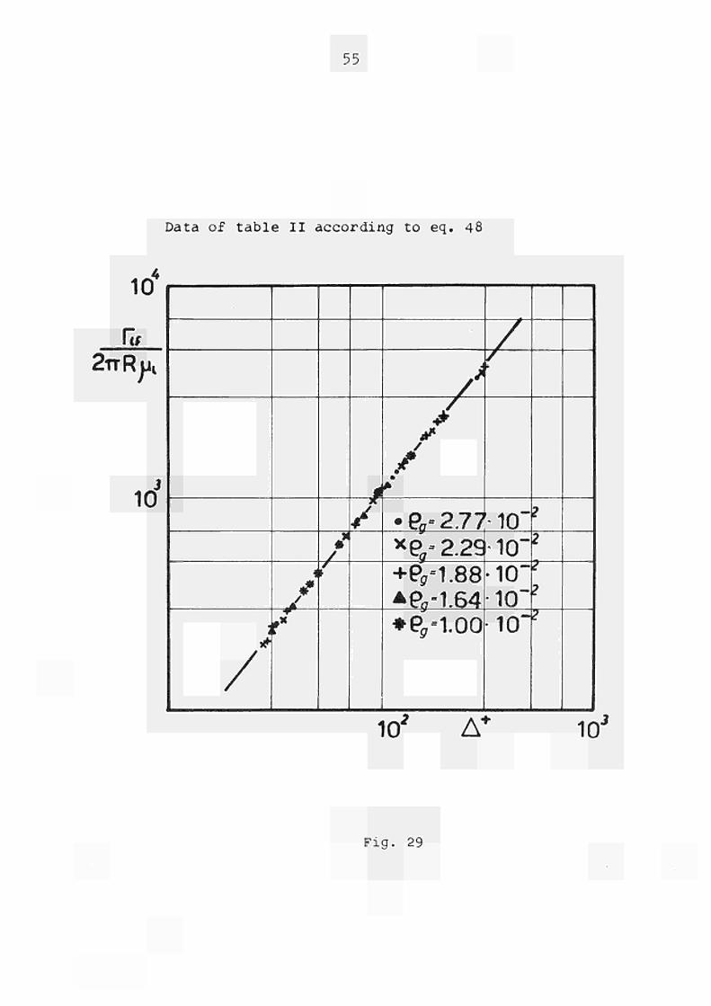
Data of table II according to eq. 48
10*
ru 2 n R ^
10J
'i
*
/
i
/ 4Γ
r* >
/ \
à
y
/
/
• »
• Çn- 2.77 xe a - 2.29
+eff-1.88
Αβ,-1.64
*ej-i.oo
/ / ■
•10" •10" •10" •10" •10"
?
2
2
2
2
10' Δ+
10J
Fig. 29
56
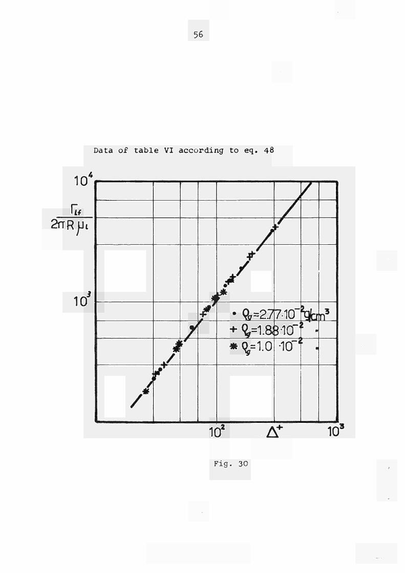
Data of table VI according to eq. 48
10*
i f
2rrRjj,
10Γ
/
X
7 . /
¿ /
Φ-Q,=277-1Q"h|b|n
:
V1.8810"
<ξ=1.0 10'
ril
10* Δ" 101
Fig . 30
57
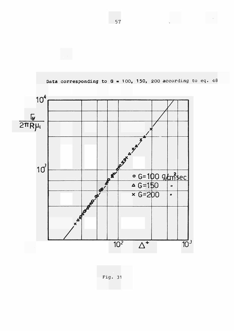
Data corresponding to G 100, 150, 200 according to eq. 48
10*
S_ 2tlRjJ,
lrf
X
/
f
à φ'
/
d
a
Ρ
*
r
»G=1í
*G=1!
* G--2
'
)og/ 30
DO
iïT?; M
m
iec
102 Δ' 10
J
F i g . 31
58
11 COMPARISON WITH HARWELL DATA
The model predictions have been compared with a set of
10/ measurements performed at Harwell
Only some data have been taken into account, because many of
them are external to the model validity range owing to the low
mass flowrate. The values of the pressure drop and the average
void fraction have been derived from experimental measurements.
This leads to some fluctuations in the predicted values as it
can be seen in fig. 3 2 where the film thickness is plotted
versus G for C| Çf Ò-~J10 \ ¡et* ■ A^c . lhe original report
gives three different film thicknesses obtained by the diffe
rent measurement techniques. The first one (f^) was calculated
from the hold up assuming that 'all the liquid is present in
the film.
The second one (FA) vus obtained by the CISE film conductance
method and the third one (F. ) by conductance probe method.
In fig. 35» also the values corresponding to p. and F- are
plotted. The model predictions seem to be well inside the strip
defined by the values of p. and F« · All the examined data are
reported in table 8°.

Comparison amongst Harwell predictions and our model.
O Model predictions <+ Holdup method Å Probe Conductance
method
O = 1.5 10« g/cm3 G =3.2 g/cm
2. sec
Δ
8
(lO"cm)
+
0
0
o A
A *
<
Ο °
A A
A
A
9/cm2sec
0
»
* 0
•
o
*
>
A i
G«
6 8 10 12 14 16 18
Fig. 32
60
12 - A SIMPLIFIED MODEL
In order to obtain some more simple analytical expressions to handle, it has also been tried to describe in another way the film and core velocity distribution. The basic assumptions of the this simplified model are the following:
a) Blasius velocity profile describes the film velocity, whilst Prandtl universal profile describes the core velocity.
b) the local void fraction exhibits a parabolic trend in the film, starting from zero at the duct wall up to a constant value o< at the film-core boundary. In the core it is assumed as constant and equal to g .
c) The local slip ratio of the film is taken equal to 1
d) It has also been assumed in the core that the dispersed liquid travels with the gas mean velocity, except for the fraction corresponding to the one billed up with the gas in the film, which has a velocity equal to the film mean velocity. According to this, one has in the film:
(49)
(50)
where t\ is equal to 0. 5 and M i s a parameter introduced so as to take into account not only linear distributions.. If S is the mean value of the void fraction, obtained, as previously said, from an existing correlation, j(*can be determined by
61
the following equation
(5 o ir R*s c xv J « V J » » J - I f 8
' - )"" ï ^
which g ive s
(52) <*\ RWOtl»!)*
(j*M)(liit<) k*+ * *{** (lmH)*- ** ImtUj
tfith this valu· of tC , it is now possible to define the film
local density 0 and the mean density f
iÁJm
(53)
(54)
The co re v e l o c i t y p r o f i l e i s g iven by
(55) U.e= UM__L|/jL".t*_£_ -iyifc
Eqs. (49) and (55) contain two undetermined constants, U
and {J : the former can be obtained by matching the veloci
ties at the filmcore boundary, the latter by means of the
balance equation on gas flowrate it ζ J4 */"* . Tnus it is
w té 4<
(56) U ï V _ - L | / J T <*_?_
• » c l · * * On the o t h e r hand, Ì* t* be ing g iven by
<4i ' * C
62
(57) ^>·^-^«Ί)ί;"(^Γ(^Γϊ-ι -
( 58) t * i* V*J# ("„-i ^ A» ) Ü'j= «Λ«" k
' S
U becomes
(59)tt.=^*fJ5f**-(-î *—Ifcí^'h4>í<
Rk+
The film thiekness Δ can be calculated by the liquid flowrate
balance equation:
(«o) ru-*h £♦£ Now, the liquid film flowrate Γ and the core liquid flowrate
Γ* on the basis of the assumption d, are:
(ei, ç»= MJLJV- ¿ ίΓΜΗΜ^Γ-'Μτ2)*^
(62) íc= ?u{irblU-**J- A ^ a t + f. A„a f
where tLfc and U. are the mean velocity in the core and in the film respectively, A^j is the film section filled up with the gas. Their expressions are
(63) ^Vij/f(^f-{-i)

63
(64)s.»i(v-±|ÍTe.i) ^ ) b * R
(ift-*)Oh*iXm+i)
(65) A oir**[ *"R _ **Å ^
*¥ v
Anti lmt-i /
Thus, substituing eqs. 61 65 in eq. (60) one obtaines
(se)
- φίο-'J-Hf^- ^)Λ}·Κ- Ì Ç*-$4*Hi·ö
in which the only unknown is the film thickness^ » Also
this equation is too complex to be analytically solved and
therefore it has been programmedon. a digital computer. The
values of and of the other quantities depending on it, pre
dicted by this simplifiée model, are shown in table $* f or m» l/à,
andine^ · As one c m see from this table and from fig. 33, the
qualitative and quantitative agreement between experimental da
ta and predicted values is satisfaction for a wide range of
values.The model predictions fail for high values ofΔ ; namely
the trend of Δ as a function of fifcat 6^ constant shows an inversion
of the dependence oní^for  values corresponding to a line
in which X is fv O.fy whilst tne trend for tne othei values
of A is correct also in the region of low t ·

64
Trend of Δ as a function o f ^ for some data of t a b l e IV.
A>102
(cm) 18
16
U
12
10
8
Ι / / /
ƒ / / / ƒ / / / ƒ / ƒ / ƒ /
ƒ /
i ' s Ι ι / Ι ι / s' 1 / s
ι / ' I / / /
/ / / / If
If / / y ^
/**
y y
y y
y
\í Gg=16
S'"G0 = 35 \
/-""" <? „---'""'
*~~~~~^ 0g = 172
= 82
1
m sec 100 200 G
ι
Fig . 33
65
APPENDIX
The shear stress f in cylindrical geometry is
By the conditions TsTc t«h l»*U and Ts T# (·Γ r*R it is
(2) c 4 - T c l > -R-kVR
( 3 ) c * * - r — T I T T ; —
thus eq. (1) becomes
(4) Icy, = — R i . Ρ + r R * - ^
or also t i l
(5) '*yi - ^r f — + —
Tpiane being equal to ( Τ , « ^ ) — * Tc , eq. (5) can be rewrit
t en
(6) Tcyl = Τ Η Β Μ * Δ Τ
Δ Τ - — ΕΓΠ? Putting now £ Τ = H t ^ - T . ^ne has
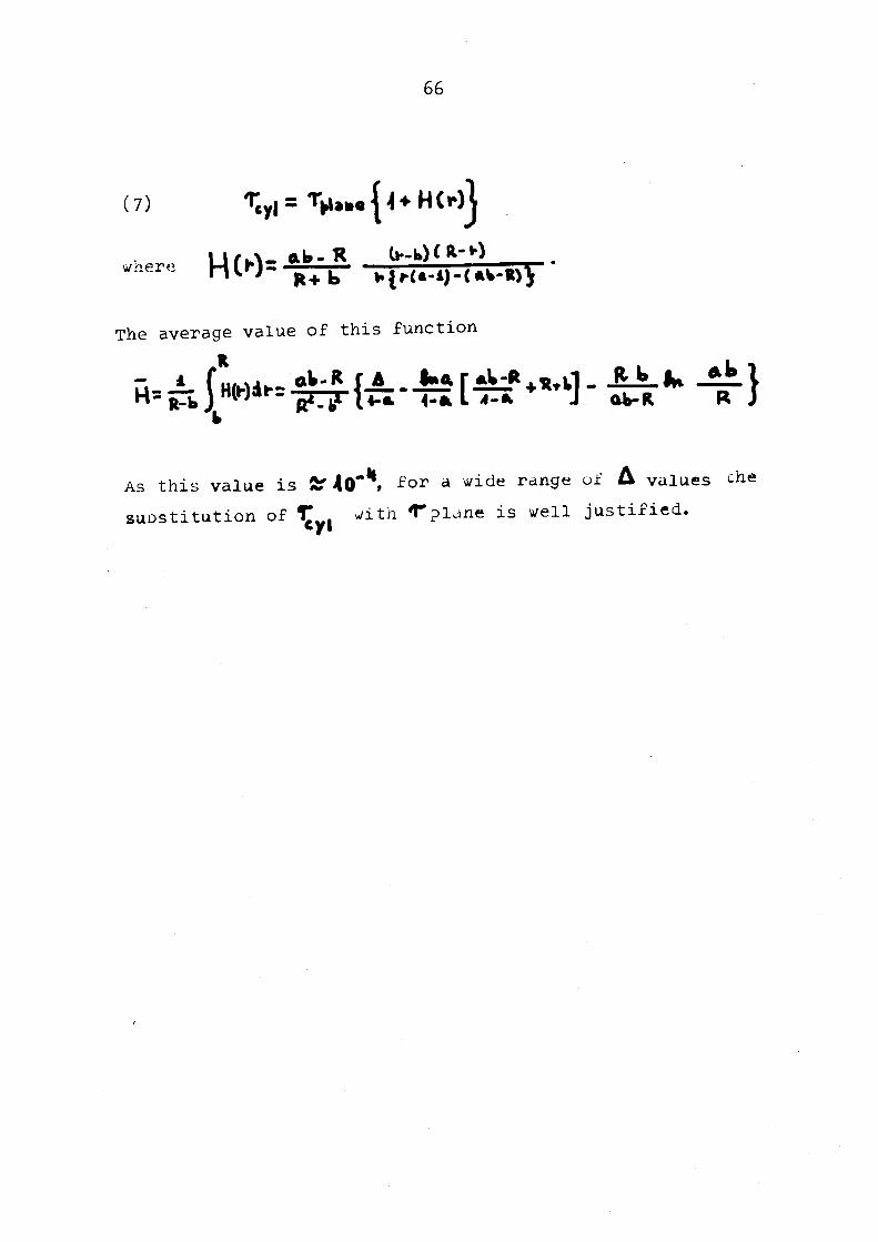
66
(7)
wnere
The average value of this function
As this value is Sf 4θ"\ for a wide range of Δ values che suDstitution of Τ with Tplane is well justified.
67
TAB. X REF. 4 Water-Ni t rogen K=1.25 cm
G
37.6
92.4
153
62.3
117.2
178.2
83.2
138
139
32.8
87.6
113.6
148.6
49.8
104.7
130.7
165.7
64.3
119.2
145.5
Χ
0.408
0.166
0.101
0.643
0.342
0.225
0.685
0.442
0.305
0.324
0.121
0.094
0.0715
0.553
0.264
0.211
0.167
0.655
0.352
0.290
As-ltf Δο·10ζ
eq.Q2)
%-■
5.65
12.9
18.3
2 .5
6 .3
8 .5
1 .64
3.56
5 .2
9r
6.05
13.8
16.4
18.6
2.81
7.25
8.5
9 .6
1 .87
4.39
5.37
277·1(Γ
4.87
9.74
13.2
2.35
3.22
5.61
1 .76
2.31
2.78
1.88-10"
5.68
12.3
15.3
18.9
2 . 9
4.31
5.69
7.91
1.75
2.90
2.98
Ac 10* *eq.G2 ? g/cm
3
4.48
10.1
18 .4
2.39
4.54
7
1.68
2.70
4.17
2 g/cm
J
4.84
11 .2
11 .2
19.9
2.82
5.57
6.84
8.48
1 .73
3.46
4.23
rtf
21 .8
114.33
325
22.58
74.95
16.23
19.76
50.81
108
21 .39
123.77
207.95
346.6
25.08
91 .6
133.5
197.32
18.46
64.98
93.36
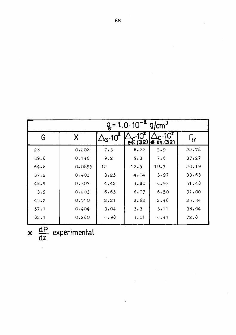
68
G
28
3 9 . 8
6 4 . 8
37 .2
4 8 . 9
3 .9
4 5 . 2
57 .1
82 .1
Χ
0 .208
0 .146
0 .0895
0 .403
0 .307
0 .203
0 . 5 1 0
0 .404
0 .280
ç,= 1.0-10"*
As-102
7 .3
9 .2
12
3 .25
4 . 4 2
6 .65
2 .21
3 .04
4 . 9 8
Ac-10\ eï (32)
8.22
9 .3
1 2 . 5
4 . 0 4
4 . 8 0
6 .07
2 .62
3 .3
4 . 0 1
g/cm3
Δς·102
* eq.(32) 5 .9
7 .6
1 0 . 7
3 .97
4 . 9 3
6 . 5 0
2 . 4 8
3 .11
4 . 4 1
Γ„ 2 2 . 7 8
37 .27
2 0 . 1 9
33 .63
51 .48
91 . 0 0
2 5 . 3 4
38 .04
7 2 . 8
* íüL experimental
69
TAB. I I REF. Χ Water-Argon R = 1.25 cm O = 2 . 7 7 . 1 0 2«j/c*5
G
57.4
45.7
73.7
48.9
37.2
64.4
39.65
27.96
113.9
58.7
161 .4
100.8
45.9
146.2
86.2
31 .2
X
0.410
0.515 0.206
0.310
0.408
0.0915
0.148
0.258
0.327
0.625
0.151
0.242
0.330
0.063
0.106
0.295
Δ5102
2.99
2.41
6 . 4
4.43
3.47
12.9
8 .7
6.65
4.71
1.91
3.34
7.41
2.91
16.9
13.7
6.31
Δε·ιο2
3.05
2.42
6.10
4.88
3.91 10.61
7.19
6.18
3.71
1 .87
8.99
5.94
2.95
20.46
11 .76
4.97
Vu
51.022
33.15 90.08
37.72
30.81
69.80
20.36
209.01
97.51 25.62
352.40
127.75 20.80
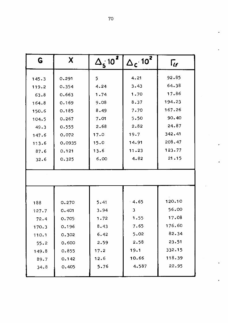
70
G
145.3 119.2
63.8
164.8
150.6
104.5
49.3
147.6
113.6
87.6
32.6
188
127.7
72.4
170.3
110.1
55.2
149.8
89.7 34.8
Χ
0.291
0.354
0.663
0.169
0.185
0.267
0.555 0.072
0.0935 0.121
0.325
0.270
0.401
0.705 0.196
0.302
0.600
0.855 0.142
0.405
As10a
5
4.24
1.74
9.08
8.49
7.01
2.68
17.0
15.0
13.6
6.00
5.41
3.94
1.72
8.43 6.42
2.59
17.2
12.6
5.76
Δ 0 10 2
4.21
3.43
1 .70
8.37
7.70
5.50
2.82
19.7
14.91
11.23
4.82
4.65
3
1.55
7.65 5.02
2.58
19.1 10.66
4.587
r« 92.85 64.38
17.86
194.23 167.26
90.40
24.87
342.41
208.47
123.77
21 .15
120.10
56.00
17.08
176.60
82.34
23.51
332.15
118.39
22.95
71
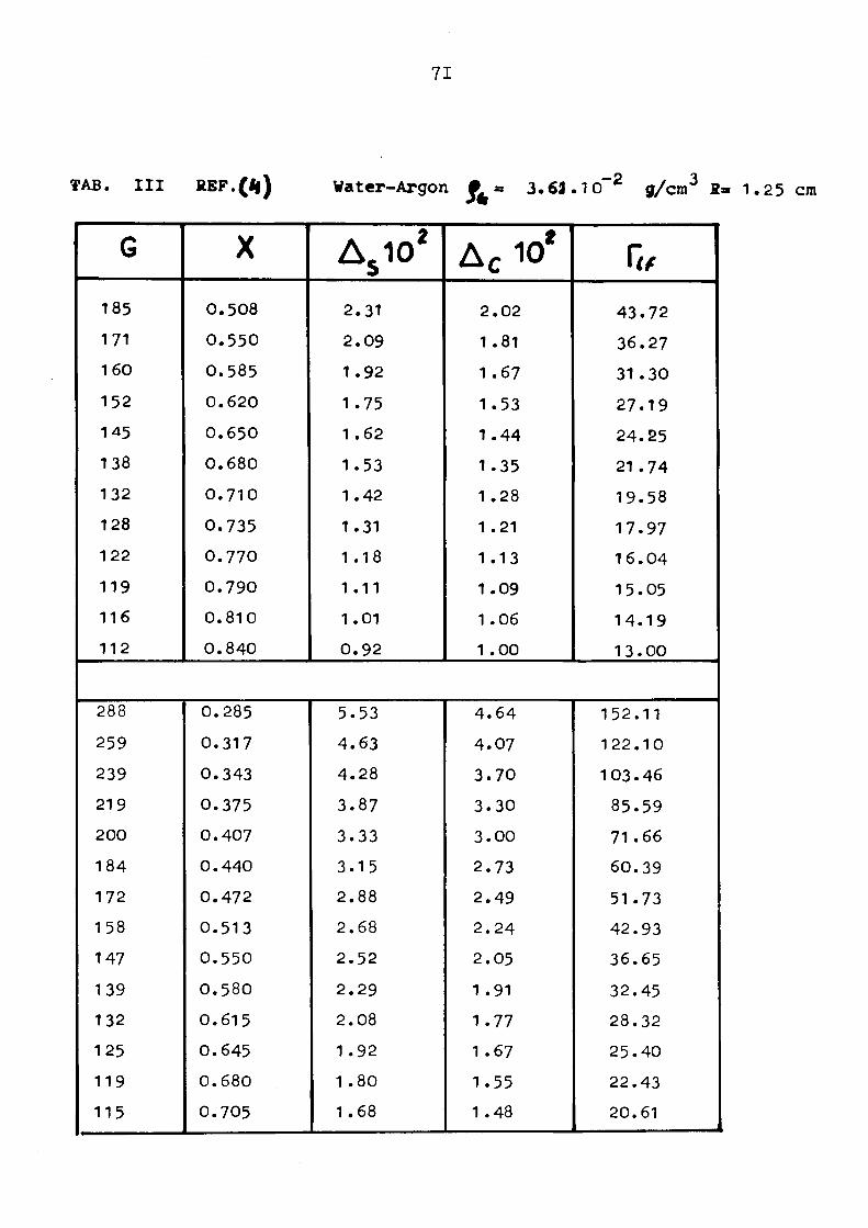
TAB. III REF. (If) Water-Argon · ■ 3.63.10~2 g/cm
3 fi» 1.25 cm
G
185
171
160
152
145
138
132
128
122
119
116
112
X
0.508
0.550
0.585
0.620
0.650
0.680
0.710
0.735
0.770
0.790
0.810
0.840
Δ5102
2.31
2.09
1 .92
1.75
1 .62
1.53
1.42
1.31
1 .18
1 .11
1.01
0.92
A c 10*
2.02
1 .81
1 .67
1.53
1.44
1.35
1 .28
1 .21
1 .13
1 .09
1 .06
1 .00
Vit
43.72
36.27
31.30
27.19
24.25
21.74
19.58
17.97
16.04
15.05
14.19
13.00
288
259
239
219
200
184
172
158
147
139
132
125
119
115
0.285
0.317
0.343
0.375
0.407
0.440
0.472
0.513
0.550
0.580
0.615
0.645
0.680
0.705
5.53
4.63
4.28
3.87
3.33
3.15
2.88
2.68
2.52
2.29
2.08
1 .92
1 .80
1.68
4.64
4.07
3.70
3.30
3.00
2.73
2.49
2.24
2.05
1 .91
1.77
1 .67
1.55
1 .48
152.11
122.10
103.46
85.59
71 .66
60.39
51.73
42.93
36.65
32.45
28.32
25.40
22.43
20.61
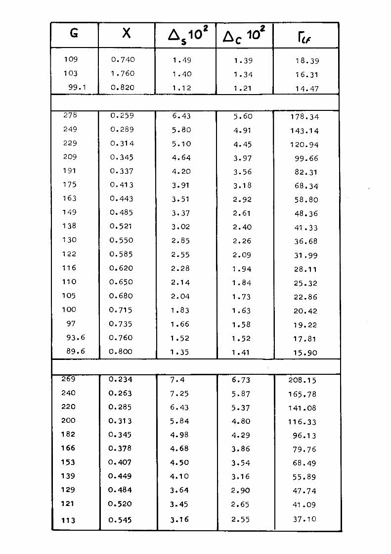
G
109
103
99.1
Χ
0.740
1 .760
0.820
Δ5102
1 .49
1 .40
1 .12
Δ 010
2
1.39
1.34
1 .21
Γ < ,
18.39
16.31
14.47
278
249
229
209
191
175
163
149
138
130
122
116
110
105
100
97
93.6
89.6
0.259
0.289
0.314
0.345
0.337
0.413
0.443
0.485
0.521
0.550
0.585
0.620
0.650
0.680
0.715
0.735
0.760
0.800
6.43
5.80
5.10
4.64
4.20
3.91
3.51
3.37
3.02
2.85
2.55
2.28
2.14
2.04
1 .83
1 .66
1.52
1.35
5.60
4.91
4.45
3.97
3.56
3.18
2.92
2.61
2.40
2.26
2.09
1 .94
1 .84
1.73
1 .63
1 .58
1.52
1.41
178.34
1 43.14
120.94
99.66
82.31
68.34
58.80
48.36
41 .33
36.68
31.99
28.11
25.32
22.86
20.42
19.22
17.81
15.90
2¿9
240
220
200
182
166
153
139
129
121
113
0.234
0.263
0.285
0.313
0.345
0.378
0.407
0.449
0.484
0.520
0.545
7 . 4
7.25
6.43
5.84
4.98
4.68
4.50
4.10
3.64
3.45
3.16
6.73
5.87
5.37
4.80
4.29
3.86
3.54
3.16
2.90
2.65
2.55
208.15
165.78
141 .08
116.33
96.13
79.76
68.49
55.89
47.74
41 .09
37.10
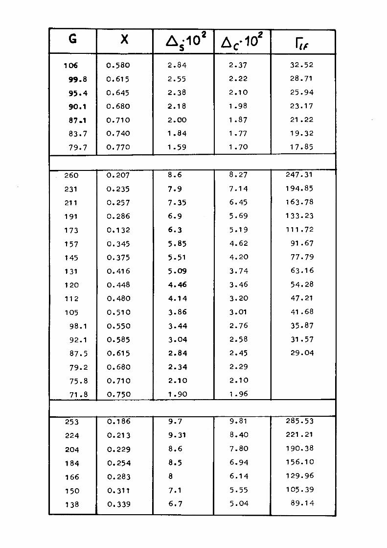
G
106
99.8
95.4 90.1
87-1 83.7
79.7
Χ
0.580
0.615
0.645 0.680
0.710
0.740
0.770
Δ5 ·102
2.84
2.55 2.38
2.18
2.00
1 .84
1.59
Δ 0 ·10 2
2.37
2.22
2.10
1 .98
1 .87
1.77
1 .70
Γ« 32.52
28.71
25.94
23.17
21 .22
19.32
17.85
260
231
211
191
173
157
145
131
120
112
105
98.1
92.1
87.5
79.2
75.8
71.8
253
224
204
184
166
150
138
0.207
0.235
0.257 0.286
0.132
0.345
0.375 0.416
0.448
0.480
0.510
0.550
0.585
0.615
0.680
0.710
0.750
8 . 6
7 . 9
7.35
6 . 9
6 . 3
5.85
5.51
5.09 4.46
4.14
3.86
3.44
3.04
2.84
2.34 2.10
1.90
8.27
7.14
6.45
5.69
5.19
4.62
4.20
3.74
3.46
3.20
3.01
2.76
2.58
2.45
2.29
2.10
1 .96
247.31
194.85
163.78
133.23
111.72
91.67
77.79
63.16
54.28
47.21
41 .68
35.87
31.57
29.04
0.186
0.213
0.229
0.254
0.283
0.311
0.339
9 . 7
9.31
8 . 6
8 .5
8
7.1
6 . 7
9.81
8.40
7.80
6.94
6.14
5.55
5.04
285.53 221 .21
190.38
156.10
129.96
105.39
89.14
G
1 1 3
105
9 7 . 6
9 0 . 8
8 4 . 8
75 .1
72 .1
6 8 . 7
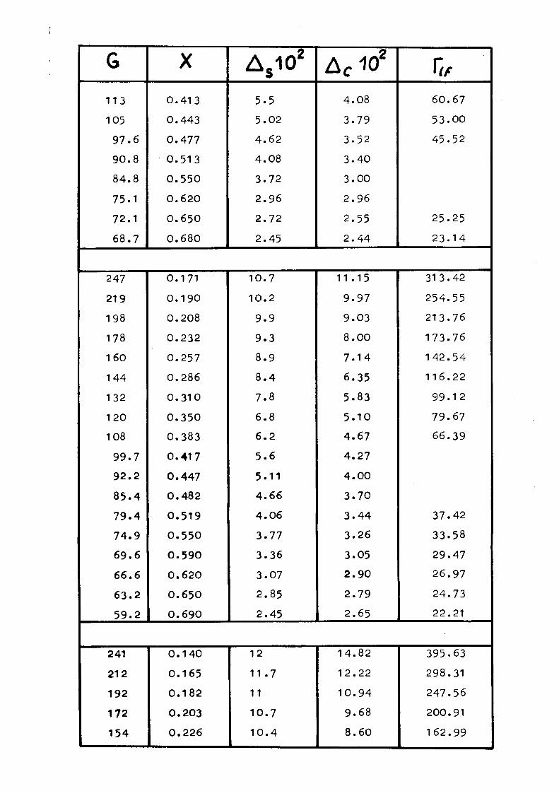
247
219
198
178
1 6 0
1 4 4
132
1 2 0
108
9 9 . 7 9 2 . 2
8 5 . 4
7 9 . 4
7 4 . 9
6 9 . 6
6 6 . 6
6 3 . 2
5 9 . 2
Χ
0 . 4 1 3
0 . 4 4 3
0 .477
0 . 5 1 3 0 . 5 5 0
0 . 6 2 0
0 . 6 5 0
0 . 6 8 0
Δ$102
5 . 5
5 .02
4 . 6 2
4 . 0 8
3 .72
2 . 9 6
2 . 7 2
2 . 4 5
Ac102
4 .08
3 .79
3 .52
3 . 4 0
3 . 0 0
2 . 9 6
2 . 5 5
2 . 4 4
Γ„ 6 0 . 6 7
5 3 . 0 0
4 5 . 5 2
2 5 . 2 5
2 3 . 1 4
0 .171
0 . 1 9 0
0 .208
0 .232
0 .257
0 .286
0 . 3 1 0
0 . 3 5 0
0 . 3 8 3
0 .417
0 .447 0 . 4 8 2
0 . 5 1 9 0 . 5 5 0
0 . 5 9 0
0 . 6 2 0
0 . 6 5 0
0 . 6 9 0
1 0 . 7
1 0 . 2
9 . 9
9 . 3
8 . 9
8 . 4
7 . 8
6 . 8
6 . 2
5 . 6
5.11 4 . 6 6
4 . 0 6
3 .77
3 . 3 6
3 .07
2 . 8 5
2 . 4 5
11 .15
9 .97
9 . 0 3
8 . 0 0
7 . 1 4
6 .35
5 . 8 3
5 . 1 0
4 . 6 7
4 . 2 7
4 . 0 0
3 . 7 0
3 . 4 4
3 . 2 6
3 .05 2 . 9 0
2 . 7 9
2 . 6 5
3 1 3 . 4 2
254 .55
213 .76
1 7 3 . 7 6
1 4 2 . 5 4
1 1 6 . 2 2
9 9 . 1 2
7 9 . 6 7
6 6 . 3 9
3 7 . 4 2
3 3 . 5 8
2 9 . 4 7
2 6 . 9 7
2 4 . 7 3
22 .21
241
212
1 9 2
1 7 2
1 5 4
0 . 1 4 0
0 .165
0 . 1 8 2
0 . 2 0 3
0 . 2 2 6
12
1 1 . 7
11
1 0 . 7
1 0 . 4
1 4 . 8 2
1 2 . 2 2
1 0 . 9 4
9 .68
8 .60
3 9 5 . 6 3
298.31
247 .56
200.91
1 6 2 . 9 9
G
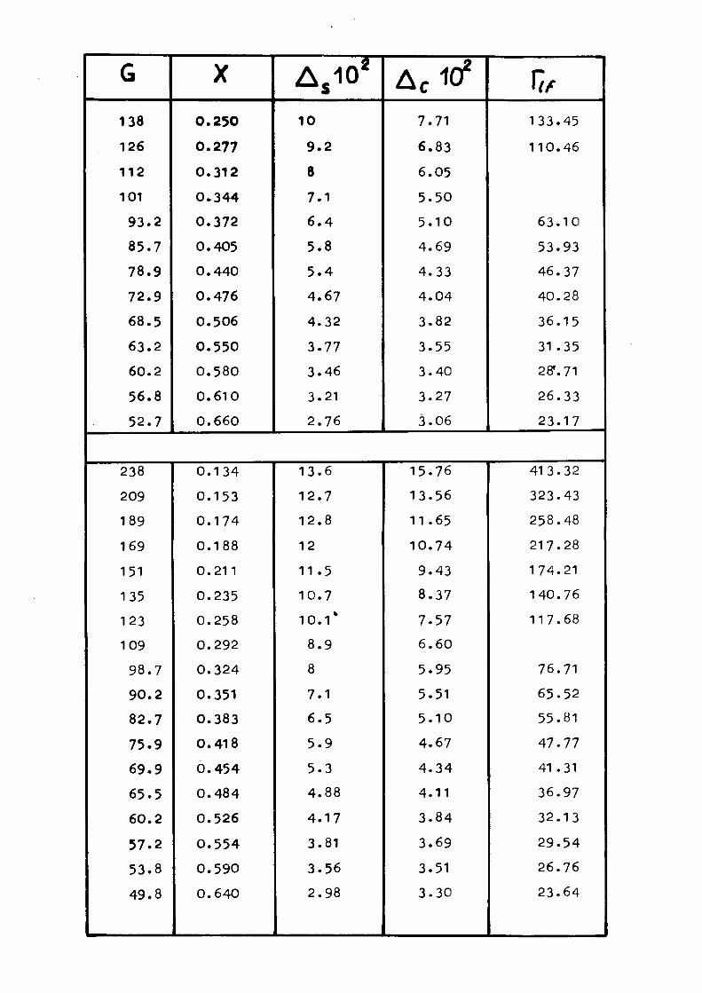
138
126
112
101
93.2
85.7
78.9
72.9
68.5
63.2
60.2
56.8
52.7
Χ
0.250
0.277 0.312
0.344 0.372
0.405
0.440
0.476
0.506
0.550
0.580
0.610
0.660
Δ5102
10
9 . 2
8
7.1
6 . 4
5 .8
5 . 4
4.67
4.32
3.77
3.46
3.21
2.76
Δ ^ Ο 2
7.71
6.83
6.05
5.50
5.10
4.69
4.33
4.04
3.82
3.55
3.40
3.27
3.06
Ttf 133.45
110.46
63.10
53.93
46.37
40.28
36.15
31 .35
28\ 71
26.33
23.17
238
209
189
169
151
135
123
109
98.7 90.2
82.7
75.9
69.9
65.5
60.2
57.2
53.8
49.8
-,
0.134
0.153
0.174
0.188
0.211
0.235 0.258
0.292
0.324
0.351
0.383 0.418
0.454
0.484
0.526
0.554
0.590
0.640
13.6
12.7 12.8
12
11.5
10.7 1 0 . 1 *
8 .9
8
7.1
6 .5
5 . 9
5 .3
4.88
4.17
3.81
3.56
2.98
15.76
13.56
11 .65
10.74
9.43
8.37
7.57 6.60
5.95
5.51 5.10
4.67
4.34
4.11
3.84
3.69
3.51
3.30
413.32
323.43
258.48
217.28
174.21
140.76
117.68
76.71 65.52
55.81
47.77
41 .31
36.97
32.13
29.54
26.76
23.64

G
234
205
185
165
147
130
119
105
93.8
86
78.5
71.7
65.7
61 .3
56
53
49.5
45.5
Χ 0.118
0.135
0.148
0.168
0.188
0.211
0.233
0.264
0.293
0.320
0.350
0.384
0.419
0.449
0.491
0.520
0.555
0.600
Δ5102
14.4
14.1
13.6
12.8
12.5
12.0
11 .3
10.00
9.1
8 .1
7 . 4
6 .7
6 .1
5.35
4.76
4,43
3.94
3.43
Δ Γ 10 2
18.72
16.04
14.44
12.44 10.92
9.57
8.50
7.47
6.70
6.13
5.63
5.17 4.80
4.53
4.23
4.06
3.90
3.71
Π, 472.29
379.94
306.08
241 .65
193.01
153.49
123.70
98.98
80.59
68.25
57.71
48.49
42.05
37.44
32.40
29.73
26.91
24.04
230
201
181
161
143
127
115
101
90.5
82.7 75.2
68.2
62.3
57.9 ι
0.105 0.121
0.133 0.150
0.169
0.190
0.210
0.239
0.267
0.293
0.322
0.354
0.387
0.419
16.0
15.7 15 .4
14.6
13.8
13.3
12.2
10.8
9 .8
9
8 .3
7 .3
6 .5
6
21 .85 18.52
16.5
14.35
12.43
13.52
9.65 8.30
7.34
6.67
6.07
5.56
5.15
4.83
531.75
410.37 337.72
268.22
211 .13
135.62
104.05
83.20
69.62
58.05
48.61
41.51
36.61
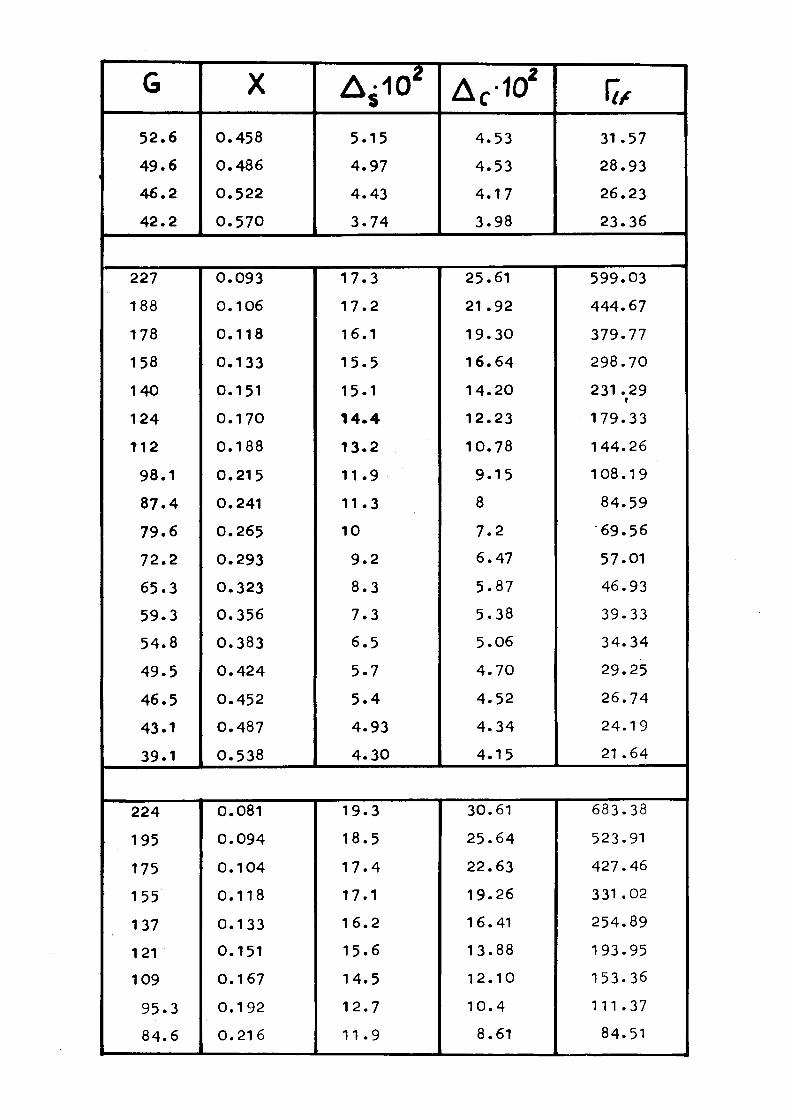
G
5 2 . 6
4 9 . 6
4 6 . 2
4 2 . 2
Χ
0 .458
0 .486
0 .522
0 .570
A¿102
5.15
4 .97
4 .43
3 .74
Δί·102
4 .53
4 .53
4 .1 7
3 .98
(7/ 31 .57
28 .93
26 .23
23 .36
227
188
178
158
140
124
112
98 .1
8 7 . 4
7 9 . 6
7 2 . 2
6 5 . 3
5 9 . 3
5 4 . 8
49 .5
46 .5
43 .1
39 .1
0 .093
0 .106
0 .118
0 .133
0 .151
0 .170
0 .188
0 .215
0 .241
0 .265
0 .293
0 .323
0 .356
0 .383
0 .424
0 .452
0 .487
0 .538
1 7 . 3
1 7 . 2
16 .1
15 .5
15 .1
1 4 . 4
1 3 . 2
1 1 . 9
11 .3
10
9 . 2
8 .3
7 .3
6 .5
5.7
5 . 4
4 .93
4 . 3 0
25 .61
21 .92
1 9 . 3 0
1 6 . 6 4
1 4 . 2 0
1 2 . 2 3
1 0 . 7 8
9 .15
8
7 . 2
6 .47
5 .87
5 .38
5 .06
4 . 7 0
4 .52
4 . 3 4
4 .15
599 .03
444 .67
379.77
298 .70
231 .29 t
179 .33
144 .26
108 .19
84 .59
69 .56
57 .01
46 .93
39 .33
34 .34
29 .25
2 6 . 7 4
24 .19
21 . 64
224
195
175
155
137
121
109
9 5 . 3
84 .6
0.081
0 .094
0 .104
0 .118
0 .133
0.151
0 .167
0 .192
0 .216
1 9 . 3
18 .5
1 7 . 4
17 .1
1 6 . 2
1 5 . 6
14 .5
1 2 . 7
11 .9
30.61
2 5 . 6 4
22 .63
19 .26
16 .41
13 .88
1 2 . 1 0
1 0 . 4
8.61
683.38
523.91
427.46
331 .02
254.89
193.95
153.36
111.37
84.51
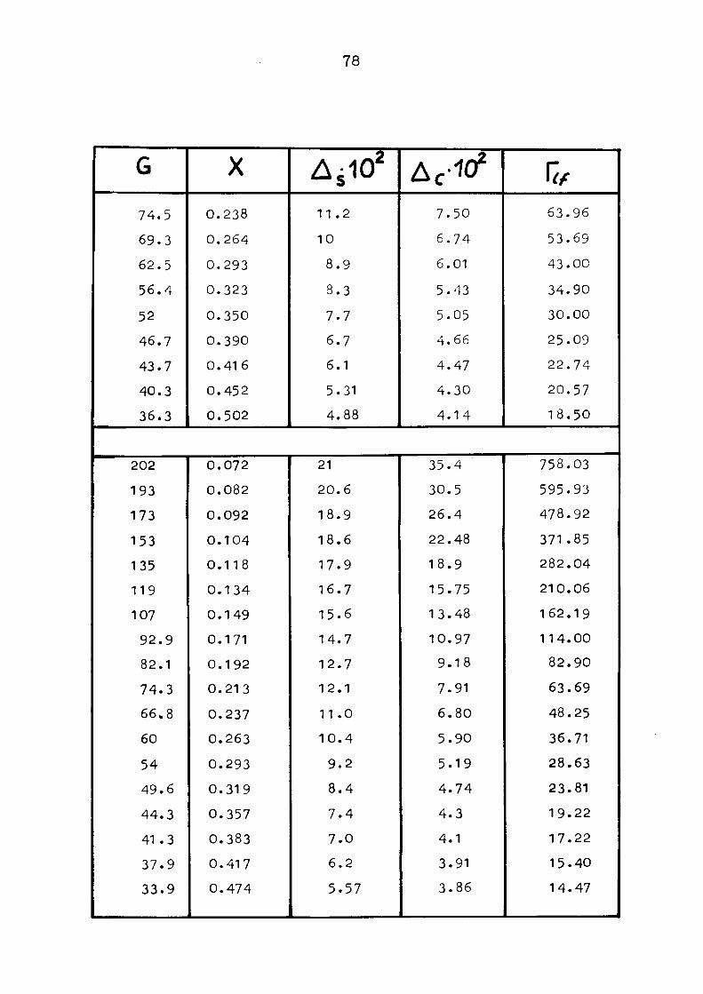
78
G
74 .5
69 .3
62 .5
5 6 . 4
52
46 .7
43 .7
40 .3
36 .3
Χ 0.238
0 .264
0.293
0 .323
0 .350
0 .390
0 .416
0 .452
0 .502
Δέ102
11 .2
10
8 .9
8.3
7 .7
6 .7
6.1
5.31
4 .88
Ac'«? 7 .50
6 .74
6.01
5 .43
5.05
4 .66
4 .47
4 . 3 0
4 . 1 4
fr
63 .96
53 .69
43 .00
34 .90
30 .00
25 .09
2 2 . 7 4
20 .57
1 8 . 5 0
202
193
173
153
135
119
107
9 2 . 9
82.1
74 .3
66 .8
60
54
49 .6
44 .3
41 .3
37 .9
3 3 . 9
0 .072
0 .082
0 .092
0 .104
0 .118
0 .134
0 .149
0.171
0 .192
0 .213
0 .237
0 .263
0 .293
0 .319
0 .357
0 .383
0 . 41 7
0 .474
21
2 0 . 6
1 8 . 9
1 8 . 6
1 7 . 9
16 .7
15 .6
14 .7
1 2 . 7
12 .1
11 . 0
1 0 . 4
9 .2
8 . 4
7 . 4
7 . 0
6 .2
5 .57
35 .4
30 .5
2 6 . 4
22 .48
1 8 . 9
15 .75
13 .48
10 .97
9 .18
7.91
6 .80
5 .90
5 .19
4 . 7 4
4 .3
4 .1
3.91
3 .86
758.03
595 .93
478 .92
371.85
282 .04
210.06
162 .19
114 .00
8 2 . 9 0
63 .69
48 .25
36.71
28 .63
23 .81
19 .22
17 .22
1 5 . 4 0
14 .47
79
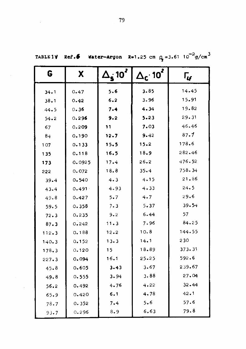
TABLE 1Y fief . f Water-Argon R»1.25 cm π =3.61 t0~"2g/cm3
G
34.1
38.1
44 .5
54.2
67
84
107
135
173
222
39.4
43.4 49.8
59.5
72.3
87.3
112.3
140.3
178.3
227.3
45.8
49.8
56.2
65.9
78.7
93.7
Χ
0.47
0.42
0.36
0.296
0.209
0.190
0.133
0.118
0.0925
0.072
0.540
0.491
0.427
0.358
0.235
0.242
0.188
0.152
0.120
0.094
0.605
0.555
0.492
0.420
0.352
0.296
Aj102
5 .6
6 . 2
7 . 4
9 . 2
11
12.7
15.5
16.5
17.4 18.8
4 . 3
4.93
5.7
7 .3
9 .2
11.3
12.2
13.3
15
16.1
3.43
3.94
4.76
6 .1
7 .4
8.9 _ _ _ _ _ _ _ _ _
Δς IO' 3.85
3.96
4.34
5.23
7.03
9.42
15.2
18.9 26.2
35.4
4.15
4 .33
4 . 7
5.37
6.44
7.96
10.8
14.1
18.89
25.25
3.67 3.88
4.22
4 .78
5.6
6.63
fr
14.45
15.91
19.82
29.31
46.46
87.7* 178.6
282.46
476.52
758.34
21.86
24.5
29.6
39.54
57
84.25
144.55
230
373.31
592.6
239.67
27.04
32.44
42.1
57.6
79.8
80
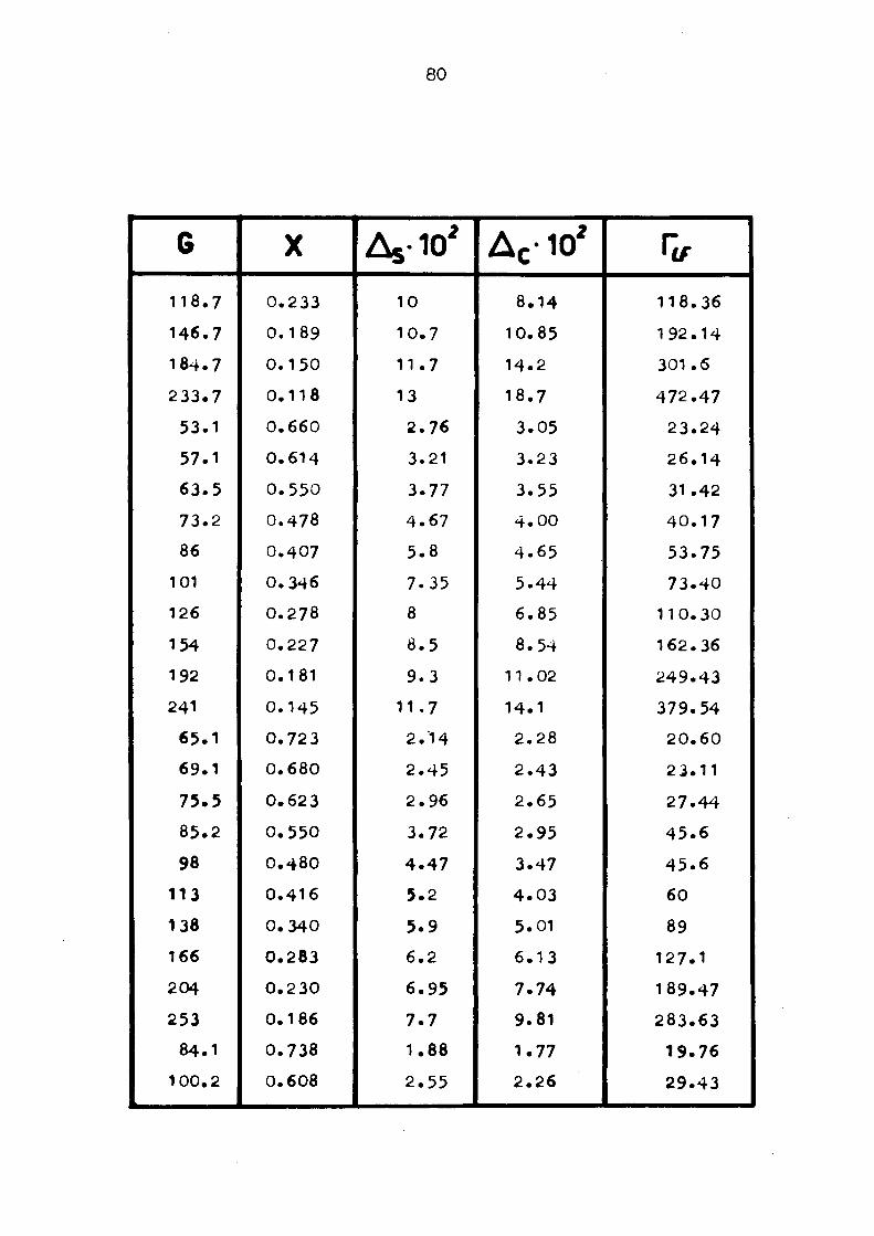
G
118.7
146.7
184.7
233.7
53.1
57.1
63.5
73.2
86
101
126
154
192
241
65.1
69.1
75.5
85.2
98
113
138
166
204
253
84.1
100.2
Χ
0.233
0.189
0.150
0.118
0.660
0.614
0.550
0.478
0.407
0.346
0.278
0.227
0.181
0.145
0.723
0.680
0.623
0.550
0.480
0.416
0.340
0.283
0.230
0.186
0.738
0.608
ΔνΙΟ2
10
10.7
11.7
13
2.76
3.21
3.77
4.67 5 .8
7.35
8
8 .5
9 .3
11.7
2.'14
2.45
2.96
3.72
4 .47
5 .2
5 . 9
6 .2
6.95
7 . 7
1.88
2.55
Δε ·1θ' 8.14
10.85
14.2
18.7
3.05
3.23
3.55
4 .00
4 .65
5.44
6.85
8.54
11.02
14.1
2.28
2.43
2.65
2.95
3.47
4 .03
5.01
6.13
7.74 9.81
1.77
2.26
fr
118.36
192.14
301 .6
472.47
23.24
26.14
31.42
40.17
53.75
73.40
110.30
162.36
249.43
379.54
20.60
23.11
27.44
45 .6
45 .6
60
89
127.1
189.47
283.63
19.76
29.43
81
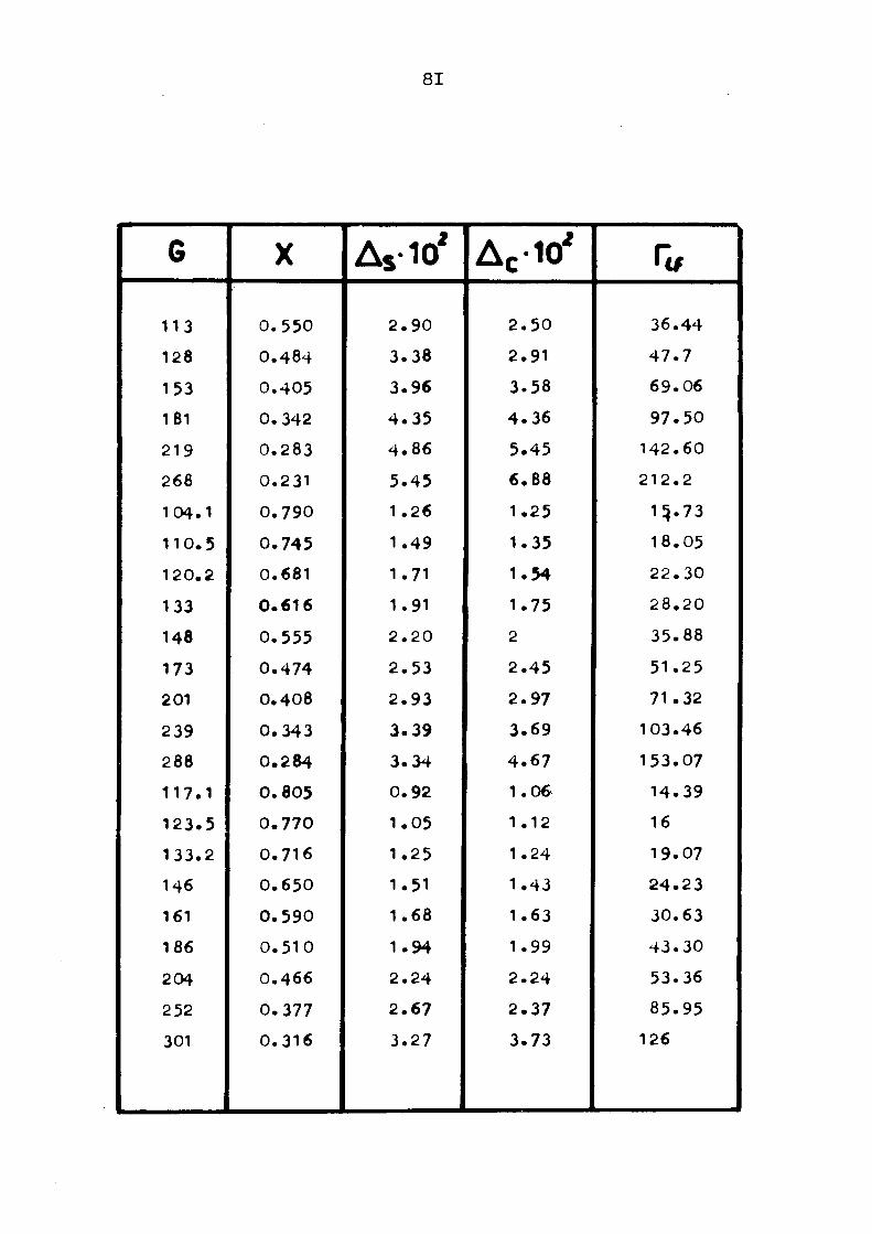
G
113
128
153
181
219
268
104 .1
1 1 0 . 5
120 .2
133
148
173
201
239
288
1 1 7 . 1
1 2 3 . 5
133 .2
146
161
186
204
2 52
301
Χ
0 . 5 5 0
0 .484
0 .405
0 . 3 4 2
0 .283
0 .231
0 . 7 9 0
0 . 7 4 5
0 .681
0 . 6 1 6
0 .555
0 . 4 7 4
0 . 4 0 8
0 .343
0 . 2 8 4
0 . 8 0 5
0 . 7 7 0
0 .716
0 . 6 5 0
0 . 5 9 0
0 . 5 1 0
0 .466
0 .377
0 .316
L· _
Δ5102
2 . 9 0
3 .38
3 .96
4 . 3 5
4 . 8 6
5 . 4 5
1 .26
1 .49
1.71
1.91
2 . 2 0
2 . 5 3
2 . 9 3
3 . 3 9
3 .34
0 .92
1 .05
1 .25
1.51
1 .68
1 .94
2 . 2 4
2 . 6 7
3 .27
Δ0·1θ'
2 . 5 0
2 . 9 1
3 .58
4 . 3 6
5 . 4 5
6 . 8 8
1.25
1.35
1.54
1 .75
2
2 . 4 5
2 . 9 7
3 .69
4 . 6 7
1 .06
1.12
1.24
1.43
1.63
1.99
2 . 2 4
2 . 3 7
3 .73
fr
3 6 . 4 4
4 7 . 7
6 9 . 0 6
9 7 . 5 0
1 4 2 . 6 0
2 1 2 . 2
15..73
1 8 . 0 5
2 2 . 3 0
2 8 . 2 0
35 .88
5 1 . 2 5
71 .32
103 .46
153 .07
1 4 . 3 9
16
19 .07
2 4 . 2 3
3 0 . 6 3
4 3 . 3 0
53 .36
8 5 . 9 5
126
82
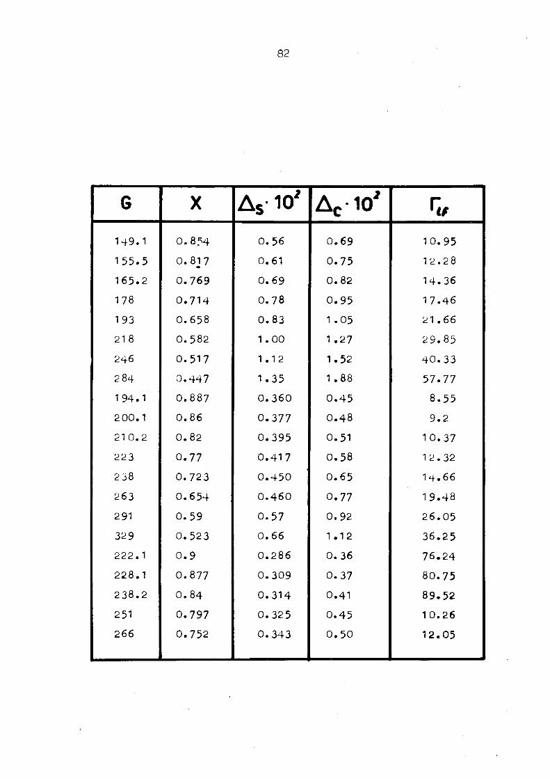
G
149 .1
1 5 5 . 5
165 .2
178
193
218
246
2 84
194.1
200 .1
210 .2
223
238
263
291
329
222 .1
228 .1
2 3 8 . 2
251
266
Χ
0 .854
0 .817
0 . 7 6 9
0 .714
0 .658
0 .582
0 .517
0 .447
0 .887
0 .86
0 .82
0 .77
0 .723
0 .654
0 . 5 9
0 .523
0 . 9
0 .877
0 . 8 4
0 .797
0 .752
Δ 5 10' 0 .56
0 .61
0 .69
0 .78
0 .83
1 .00
1.12
1 .35
0 . 3 6 0
0 .377
0 .395
0 .417
0 . 4 5 0
0 . 4 6 0
0 .57
0 .66
0 .286
0 .309
0 .314
0 .325
0 .343
Δ 0 1θ' 0 . 6 9
0 .75
0 .82
0 .95
1.05
1.27
1.52
1.88
0 . 4 5
0 .48
0 .51
0 .58
0 .65
0 .77
0 .92
1.12
0 .36
0 .37
0 .41
0 .45
0 . 5 0
fr
1 0 . 9 5
1 2 . 2 8
14 .36
17 .46
21 .66
2 9 . 8 5
4 0 . 3 3
57 .77
8 .55
9 .2
1 0 . 3 7
12 .32
14 .66
1 9 . 4 8
2 6 . 0 5
36 .25
7 6 . 2 4
8 0 . 7 5
8 9 . 5 2
1 0 . 2 6
1 2 . 0 5
83
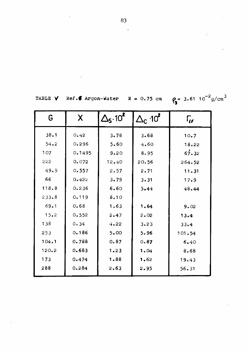
TABLE V* Ref . f A r g o n - W a t e r R = 0 . 7 5 cm O - 3 .61 10 g / - 2 / 3
■ cm
G
38.1
54 .2
1 07
222
4 9 . 9
66
11.8.8
2 3 3 . 8
69 .1
15 .2
138
253
104 .1
120 .2
173
288
X
0 .42
0 .296
0 .1495
0 .072
0 .557
0 .422
0 .236
0 .119
0 .68
0 .552
0 . 3 4
0 .186
0 .788
0 . 6 8 3
0 . 4 7 4
0 .2 84
Δ*· 10*
3.78
5 . 6 0
9 . 2 0
1 2 . 4 0
2 . 5 7
3 .79
6 . 6 0
8 . 1 0
1 . 6 3
2 . 4 7
4 . 2 2
5 . 0 0
0 . 8 7
1.23
1.88
2 . 6 3
Δς-ΙΟ* 3 .68
4 . 6 0
8 .95
2 0 . 5 6
2 .71
3 .31
5 .44
1.64
2 . 0 2
3 .23
5 .96
0 . 8 7
1 .04
1.62
2 . 9 5
&
1 0 . 7
1 8 . 2 2
67 .32
2 6 4 . 5 2
11 .31
1 7 . 9
4 8 . 4 4
9 .02
1 3 . 4
3 3 . 4
1 01 . 5 4
6 . 4 0
8 .68
1 9 . 4 3
56 .31
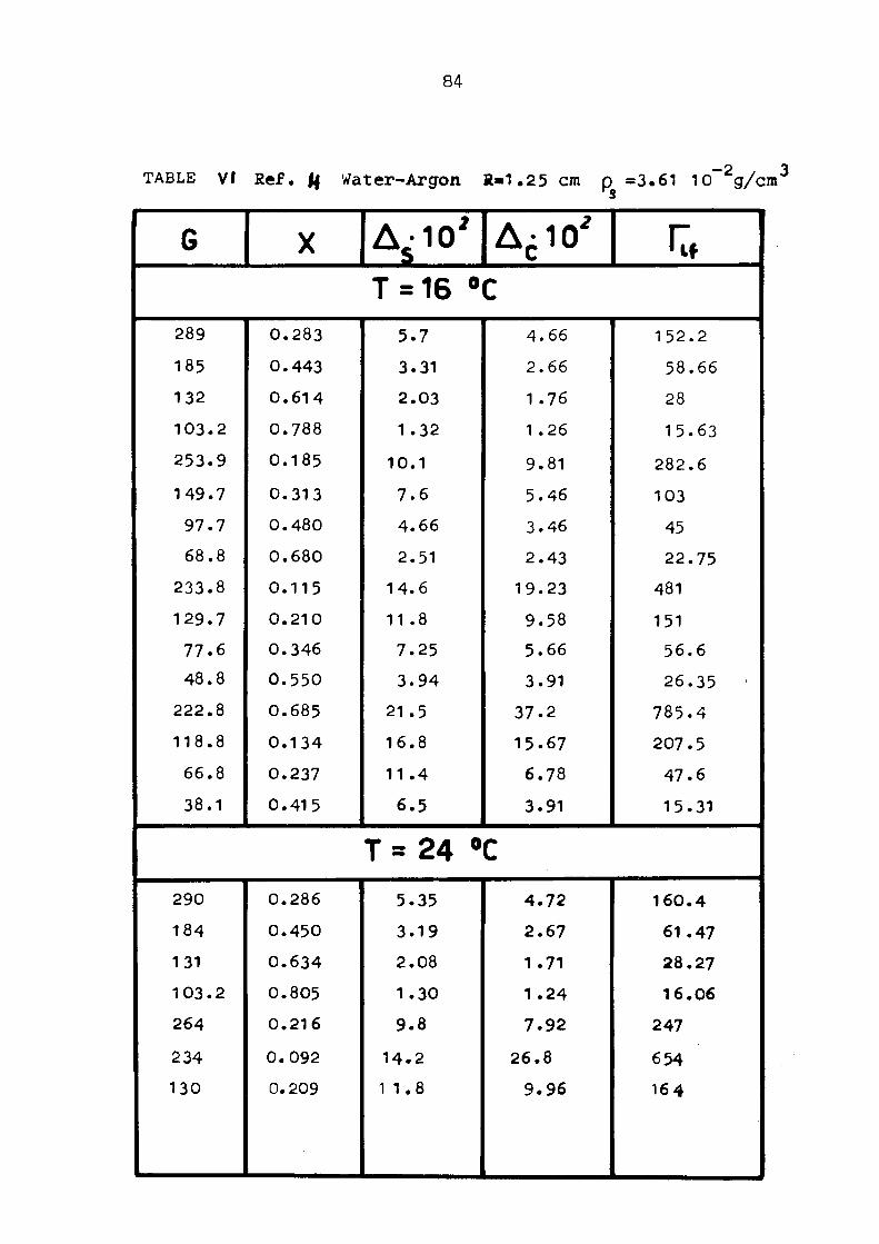
84
TABLE VI Ref. Jf Water-Argon R-1.25 cm ρ =3.61 10~2g/cm3
s
G
289
185
132
103.2
253.9
149.7
97.7 68.8
233.8
129.7 77.6 48.8
222.8
118.8
66.8
38.1
290
184
131
103.2
264
234
130
Χ
0.283
0.443
0.614
0.788
0.185
0.313
0.480
0.680
0.115
0.210
0.346
0.550
0.685
0.134
0.237
0.415
0.286
0.450
0.634
0.805 0.216
0.092
0.209
Δ;10 2
Τ =16 ° 5.7
3.31
2.03
1.32
10.1
7 .6
4.66
2.51 14.6
11 .8
7.25
3.94
21.5
16.8
11.4
6 .5
Τ =24 ° 5.35
3.19
2.08
1.30
9 .8
14.2
1 1 .8
Δ έ 1 0 ' C
4.66
2.66
1 .76
1 .26
9.81
5.46
3.46
2.43
19.23
9.58
5.66
3.91
37.2
15.67
6.78
3.91
C 4.72
2.67
1.71
1 .24
7.92
26.8
9.96
fr
152.2
58.66
28
15.63
282.6
103
45
22.75 481
151
56.6
26.35
785.4
207.5
47.6
15.31
160.4
61.47
28.27
16.06
247
654
164

G
77.9
49.1
223.1
119.1
67
38.2
X
0.349
0.554
0.072
0.135
0.239
0.420
Δ>·102
7.35
3.95 21 .7
16.3
11 .0
6 .3
Δς ·1θ'
5.80
4.01
37.01
16.06
6.96
4.07
fr
61.34
28.9
806
220
52
17.2
Τ = 30 °C 289
186
133
104.1
253.4
150.1
98
69.1
233.2
130
77.9
49
222.1
119.1
67
381
0.287 0.446
0.620
0.790
0.188
0.317
0.484
0.690
0.117
0.209
0.348
0.565
0.0725
0.135 0.240
0.424
5.15
3.06
2.00
1 .20
9 . 0
6.95
4.59
2.50
13.8
11.4
7.15 3.92
20.9
16.1
11 .0
6.15
4.79
2.75
1.79
1 .30
10.17
5.65
3.58
2.48
20
10.2
5.93 4.01
37.2
16.4
7.07
4.16
167
66
31.52
17.85
309
114.6
50.62
25.76
525
172
64.77 30.16
820
230
54.48
18.37
T=37°C 289
185
132
104.1
253.3
0.288
0.446
0.629 0.790
0.186
5.10
3.13
2.03
1 .31
9 . 4
4.87
2.82
1.79
1.32
10.6
174
69.56
32.32
19
328.65
86
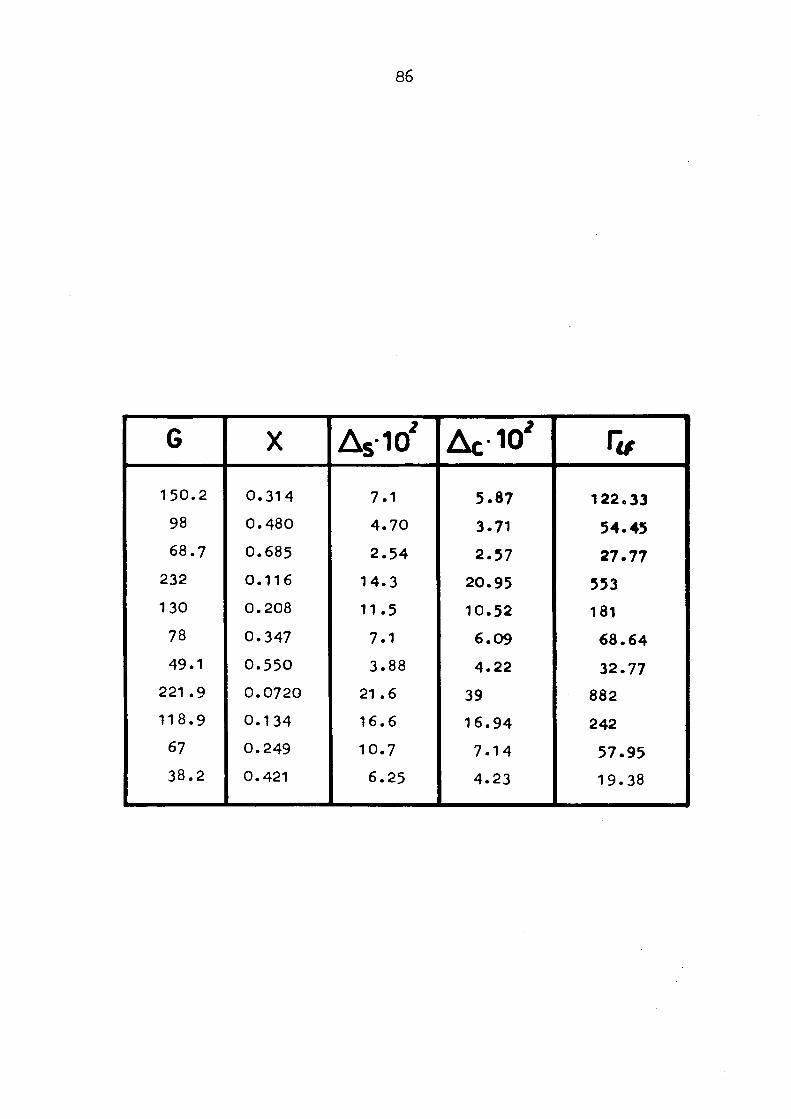
G
150.2
98
68.7
232
130
78
49.1
221 .9
118.9
67
38.2
Χ
0.314
0.480
0.685
0.116
0.208
0.347
0.550
0.0720
0.134
0.249
0.421
Δ5-102
7.1
4.70
2.54
14.3
11.5
7.1
3.88
21 .6
16.6
10.7
6.25
ΔςΙΟ'
5.87
3.71
2.57
20.95 10.52
6.09 4.22
39
16.94
7.14
4.23
fr
122.33
54.45
27.77
553
181
68.64
32.77 882
242
57.95 19.38
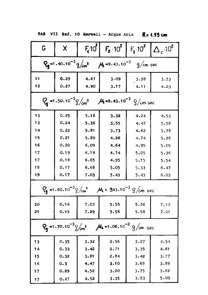
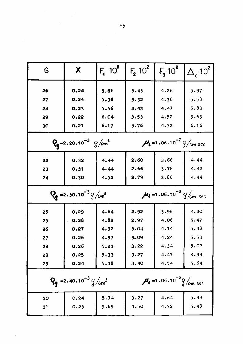
TAB VII Kef. 10 Härveli - Acqua Aria Rs 4.5S On
G
V 11
12
V 13
13
14
15
16
17
17
18
19
?,-i
20
21
V1
13
14
15
16
17
17
X çicf F2 102
'*°·ΛΟ
~\/θα} / t «9.43.10
0.29
0.27
4.67
4.90
3.09
3.17
•50
-10
"3o
)/cm
3 A -
9·
4 3·
1 0
0.25
0.24
0.22
0.21
0.20
0.19
0.18
0.17
0.17
.60.1 o"3ς
0.16
0.15
.70.10~3C
0.35
0.33 0.32
0 . 3
0.29
0.27
5.18
5.38
5.81
5.89
6.09
6.19
6.65 6.68
7.03
3.32
3.55
3.73 4.26
4.64
4.74
4.95
5.05
5.43
VÍu-* A =943.10'
7.03
7.29
5.58
5.58
>¿n» A '1·
0 6·
1 0"
3.32
3.42
3.81
4.47
4.52
4.52
2.56
2.71
2.84
3.10
3.20
3.35
F,102 Δ,-10*
g/cm · sec
3.98
4.11
3.53
4.23
Ç/cm· sec
4.24
4.47
4.62
4.74
4.95
5.05
5.15
5.33
5.43
4.53
5.58
5.78
5.28
5.05
5.36
5.54
6.47
6.03
S/cm sec
5.56
5.58
7.19
7.91
3/c**· sec
3.27
3.35
3.42
3.68
3.75
3.83
4.54
4.61
3.77
3.89
3.82
5.09
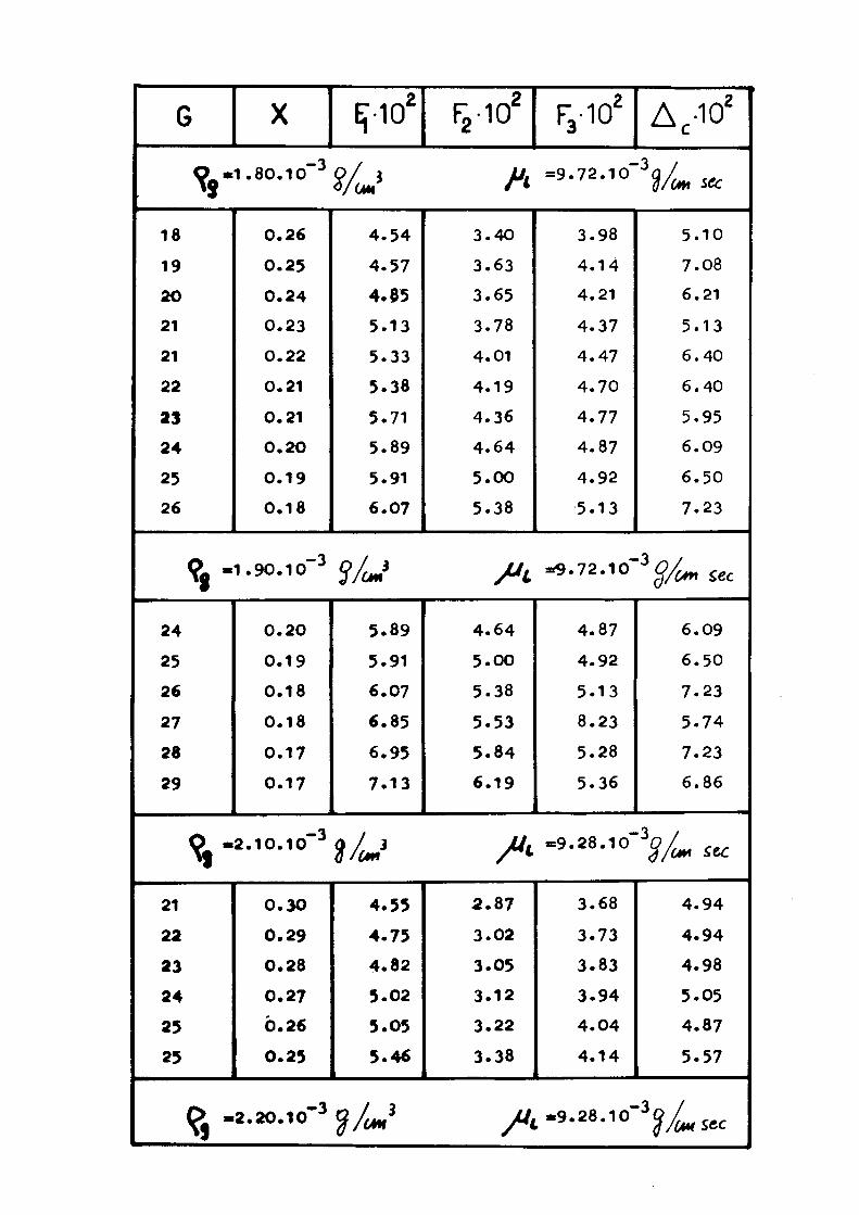
G
V 18
19
20
21
21
22
23
24
25
26
V 24
25
26
27
28
29
V 21
22
23
24
25
25
% '
X
1.80.1 θ"3
0.26
0.25
0.24
0.23
0.22
0.21
0.21
0.20
0.19
0.18
1 .90 .10"3
0.20
0.19
0.18
0.18
0.17
0.17
2 .10 .10"3
0.30
0.29
0.28
0.27
Ó.26
0.25
2 . 2 0 . 1 0 *3
E~ 10a
$/<¿
4.54
4.57
4.85
5.13
5.33
5.38
5.71
5.89
5.91
6.07
?/o»>
5.89
5.91
6.07
6.85
6.95
7.13
îU 4.55
4.75
4.82
5.02
5.05
5.46
<iUl
F2-102
h
3.40
3.63
3.65
3.78
4.01
4.19
4.36
4 .64
5.00
5.38
y"t
4.64
5.00
5.38
5.53
5.84
6.19
Λ 2.87
3.02
3.05
3.12
3.22
3.38
A
F3-102
A c -102
=9.72.10-y^ sec
3.98
4.14
4.21
4.37
4.47
4.70
4.77
4.87
4.92
5.13
5.10
7.08
6.21
5.13
6.40
6.40
5.95
6.09
6.50
7.23
=9.72.io"3ej/m €ec
4.87
4.92
5.13
8.23
5.28
5.36
6.09
6.50
7.23
5.74
7.23
6.86
e 9·
2 8·
1 0"
3^ sec
3.68
3.73
3.83
3.94
4.04
4.14
4.94
4.94
4.98
5.05
4.87
5.57
, - 9 . 2 8 . 1 0 -3
^ s e c
89
G
26
27
28
29
30
V 22
23
24
ι.
25
25
26
27
28
29
29
V 30
31
X
0.24
0.24
0.23
0.22
0.21
2.20.10"
0.32
0.31
0.30
2.30.10"
0.29
0.28
0.27 0.26
0.26
0.25
0 .24
2.40.10"
0.24
0.23
F<-10f
5.61
5.36
5.56
6.04
6.17
3 ? / ^ 4.44
4 .44
4.52
VcW 4.64
4.82
4.92
4.97
5.23
5.33 5.38
V**3
5.74
5.89
F2-102
3.43
3.32
3.43
3.53
3.76
Λ' 2.60
2.66
2.79
/ * -
2.92
2.97
3.04
3.09
3.22
3.27
3.40
Λ-3.27 3.50
F,· 10*
4.26
4.36
4.47 4.52
4.72
Δ0·102
5.97
5.58
5.83
5.65
6.16
1.06.10~ 2 J /cn , s c c
3.66 3.78 3.86
4.44
4.42
4.44
1 - 0 6 - 1 0 " 2 5 > / 4 r , sec
3.96
4.06
4.14
4.24
4.34
4.47
4.54
4.80
5.42
5.38
5.53 5.02
4.94
5.64
1 . 0 6 . 1 0 ~ 2 0 / rBr J/om sec
4.64
4.72
5.49
5.48
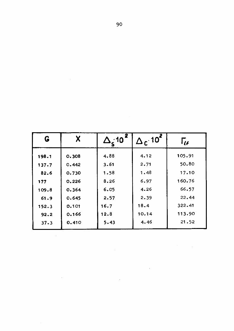
90
G
198.1
137.7 82.6
177
109.8
61.9
152.3 92.2
37.3
Χ
0.308
0.442
0.730
0.226
0.364
0.645 0.101 0.166
0.410
Δ 510 2
4.88
3.61
1.58
8.26
6.05
2.57
16.7 12.8
5.43
Δ c· 10* 4.12
2.71 1.48
6.97 4.26
2.39
18.4
10.14 4.46
fr
105.91
50.80
17.10
160.76
66.57
22.44
322.41
113.90
21 .52
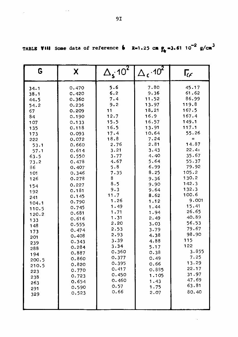
91
TABLE f i l l Some data of reference j» R-1.25 cm f ·3 .61 io" 2 g/ce3
G
3 4 . 1 3 8 . 1 4 4 . 5 5 4 . 2 67 84 107 135 173 222
53 .1 57 .1
6 3 . 5 7 3 . 2 86 101 126
154 192 241 104 .1 1 1 0 . 5 1 2 0 . 2 1 33 148 173 201 239 288 194 200 .5 210 .5 223 238 263 291 329
X
0 . 4 7 0 0 . 4 2 0 0 . 3 6 0 0 .236 0 .209 0 .190 0 .133 0 .118 0 .093 0 .072 0 .660 0 . 6 1 4 0 .550 0 .478 0 .407 0 .346 O.278 0 .227 0.181 0 .145 0 . 7 9 0 0 .745 0 .681 0 .616 0.-555 0 . 4 7 4 0 .408 0 .343 0 . 2 8 4 0 .887 0 . 8 6 0 0 . 8 2 0 0 .770 O.723 0 . 6 5 4 0 .590 O.523
Δ5·102
5 .6 6 . 2 7 . 4 9 . 2
11 1 2 . 7 1 5 . 5 1 6 . 5 1 7 . 4 1 8 . 8
2 .76 3.21 3 .77 4 .67 5 .8 7 .35 8 8 .5 9 .3
1 1 . 7 1 .26 1 .49 1 .71 1 .31 2 . 2 0 2 .53 2 .93 3 .39 3 . 3 4 0 . 3 6 0 0 .377 0 .395 0 .417 0 .450 0 .460 0 .57 0 .66
Afrf 7 . 8 0 9 .36
11 .52 13 .97 18 ,21 1 6 . 9 16 .57 13 .91 1 0 . 6 4
7 -24 2 .81 3 .43 4 . 4 0 5 . 6 4 6 .99 8 .25 9 .36 9 . 9 0 9 . 6 4 8 .62 1 .12 1 . 4 4 1 . 94 2 .49 3 .03 3 .79 4 .38 4 .88 5 .17 0 .38 0 .49 0 .66 0 .885 1 .105 1 .43 1.75 2 .07
fr
45 .17 61 .62 86 .99
119 .8 167 .5 1 6 7 . 4 149 .1 117 .1
55 .26 =
14 .87 22.41 35 .67 55 .37 79 .92
105 .2 130 .2 142 .3 132 .3 1 0 0 . 6
9 .001 15-41 26.65 40 .89 56 .53 79 .67 9 8 . 9 0
115 122
3-855 7.25
13 .29 22 .17 31 .97 47 .69 63 .81 80 .40
92
BIBLIOGRAPY
1 -- S. Levy ; "Prediction of Two-Phase Annular Flow with liquid Entrainment", Int. J. Heat Mass Tranfer Vol. 9 pp. 171-188 1966.
2 - L. Cravarolo A. Hassid: "Phase and velocity distribution in two-phase adiabatic dispresed flow", CISE Repord NO. 98
3 - I. P. Ginzburg; "Applied Fluid Dynamics", Israel Program for Scientific Translation - Jerusalem 1963
4 - "A Research program in two-phase flow", CISE - Gennaio 1963
5 - N. Adorni at ¿1 - "Experimental data on two-phase adiabatic flow: liquid film thickness, phase and velocity distribution, pressure drop in vertical gas-liquid flow? CISE Report NO. 35
6 - P. Alia - L. Cravarolo - A. Hassid - E. Pedrocchi; " Phase and velocity distribution in two-phase annular dispersed flow", CISE Report R. - 109 Dicembre 1966
7 - G. P. Gaspari - C. Lombardi - G. Peteriongo: "Pressure drop in s team-water mixtures. Round tubes. Vertical up flow", CISE Report - R - 83 gennaio 1964
8 - P. Alia - L. Cravarolo - A. Hassid a. E. Feàroochj.:· "Liquid volume fraction in adiabatic two-phase vertical up flow-round conduit", CISE Report R - 105 Giugno 1965
9 - G. F. Hewitt : Private comunication at Round Table of the European two-phase Flow Group, June 1966.
1 0 - G.F. Hewitt - P.C. Lovegrove : *Comparative Fil» thickness and Hold up measurements in vertical Annular Flow" AERE -M 1203 - 1S63

93
ACKNOWLEDGMENTS
We gratefully acknowledge the many useful discussions
with Professor M. Silvestri, who gave his time
generously, during the development of the research.
We want also to thank Mr. Gaspari and Mr. Hassid vho
allowed us to utilize their more recent experimental data,


I To disseminate knowledge is to disseminate prosperity — I mean
I general prosperity and not individual riches — and with prosperity
: disappears the greater part of the evil which is our heritage from
I darker times.
M ^ l î - î f i S S i î
vtmuì
Alfred Nobel
*Ä__5P? ι måat W B-!!åy,

æfiLti
tiSMàvïî
iwwtäK
SALES OFFICES
All Euratom reports are on sale at the offices listed below, at the prices given on the back of the front cover (when ordering, specify clearly the EUR number and the title of the report, which are shown on the front cover).
OFFICE CENTRAL DE VENTE DES PUBLICATIONS
DES COMMUNAUTES EUROPEENNES
2, placo de Metz, Luxembourg (Compte chèque postal N° 191-90)
BELGIQUE — BELGIË
MONITEUR BELGE 40-42, rue de Louvain - Bruxelles BELGISCH STAATSBLAD Leuvenseweg 40-42, - Brussel
L U X E M B O U R G
OFFICE CENTRAL D E VENTE DES PUBLICATIONS DES COMMUNAUTES E U R O P E E N N E S 9, n ie Goethe - Luxembourg
tWSW
DEUTSCHLAND
BUNDESANZEIGER Postfach - Köln 1
FRANCE
SERVICE D E VENTE EN FRANCE DES PUBLICATIONS DES COMMUNAUTES E U R O P E E N N E S 26, rue Desaix - Paris 15e
NEDERLAND
STAATSDRUKKERIJ Christoffel Plantijnstraat - Den Haag
PSiM
ITALIA
L I B R E R I A DELLO STATO Piazza G. Verdi, 10 - Roma
U N I T E D KINGDOM
H. M. STATIONERY OFFICE P . O. Box B69 - London S.E.I
EURATOM — C.I.D. 51-53, rue Belliard Bruxelles (Belgique)
CDNA03765ENC ■