Studies of Aggregation Pathways for Amyloidogenic Peptides ... · Studies of Aggregation Pathways...
246
Studies of Aggregation Pathways for Amyloidogenic Peptides by Dielectric Relaxation Spectroscopy Donald E. Barry, Jr. A Dissertation Submitted to the Faculty of Worcester Polytechnic Institute in partial fulfillment of the requirements for the Degree of Doctor of Philosophy in Physics April 2013 APPROVED: Izabela R.C. Stroe, Assistant Professor of Physics, WPI, PhD Advisor Germano S. Iannacchione, Department Head & Associate Professor of Physics, WPI David C. Medich, Assistant Professor of Physics, WPI Florin Despa, Assistant Professor, Dept. of Pharmacology, Univ. of California, Davis
Transcript of Studies of Aggregation Pathways for Amyloidogenic Peptides ... · Studies of Aggregation Pathways...

Studies of Aggregation Pathways for Amyloidogenic Peptides by
Dielectric Relaxation Spectroscopy
Donald E. Barry, Jr.
A Dissertation
Submitted to the Faculty of
Worcester Polytechnic Institute
in partial fulfillment of the requirements for the
Degree of Doctor of Philosophy
in
Physics
April 2013
APPROVED:
Izabela R.C. Stroe, Assistant Professor of Physics, WPI, PhD Advisor
Germano S. Iannacchione, Department Head & Associate Professor of Physics, WPI
David C. Medich, Assistant Professor of Physics, WPI
Florin Despa, Assistant Professor, Dept. of Pharmacology, Univ. of California, Davis

c© Copyright by Donald E. Barry, Jr., 2013.
All rights reserved.
Abstract
Diseases associated with amyloid aggregation have been a growing focus of medical
research in recent years. Altered conformations of amyloidogenic peptides assemble to
form soluble aggregates that deposit into the brain and spleen causing disorders such
as Alzheimer’s disease and Type II diabetes. Emergent theories predict that fibrils
may not be the toxic form of amyloidogenic structures and that smaller oligomer and
protofibril aggregates may be the primary source of cellular function damage.
Studies show that these amyloidogenic aggregates are characterized by an in-
creased number of poorly dehydrated hydrogen backbones and large surface densities
of patches of bulk like water which favor protein association. When proteins aggre-
gate to form larger structures, there is a redistribution of water surrounding these
proteins. The water dynamics of amyloidogenic aggregation is different than the
monomeric form and has a decrease in the number of patches occupied by molecules
with bulk-like water behavior. We demonstrate that the redistribution of water dur-
ing amyloid aggregation is reflected in a change in the dielectric relaxation signal of
protein-solvent mixtures.
We use dielectric relaxation spectroscopy (DRS) as a tool for studying the dy-
namics of amyloidogenic peptides—amyloid beta (Aβ1−42) and human islet amyloid
polypeptide (hIAPP)—during self-assembly and aggregation. Non-amyloidogenic
analogs—scrambled Aβ42−1 and rat islet amyloid polypeptide (rIAPP)—were used
as controls. We first present studies of amyloidogenic peptides in a deionized water
buffer at room temperature as a function of concentration and incubation time. From
this we were able to determine differences in amyloidogenic and non-amyloidogenic
peptides through the dielectric modulus. We next present the same analytes in a
deionized water-glycerol buffer to facilitate the study of the dielectric permittivity
at sub-freezing temperatures and model the kinetics of the α-and β-relaxation pro-
cesses. We conclude our work by studying the peptides in a bovine serum albumin
iii

(BSA) and glycerol buffer to demonstrate dielectric spectroscopy as a sensitive tool
for measuring amyloidogenic peptides in an in vivo-like condition.
iv

Acknowledgements
First and foremost I would like to thank my family. To my parents, Donald and
Susan Barry who who have always supported and inspired me to pursue a career in
science. To my wife, Romiya who has been crucial in my successes through her love,
encouragement, and unwavering support. I am so very lucky to have you in my life.
I give very special thanks to Dr. W. Peter Hansen and Dr. Petra Krauledat.
Not only have you been employers and mentors, you have also been great friends.
I tremendously appreciate the support you have given me throughout my graduate
studies. Your guidance over the last ten years has helped mold me into the researcher
and leader that I am today.
I would like to thank my advisor, Dr. Izabela Stroe for her enthusiasm and
mentoring throughout my dissertation work. The origins of this project lies in your
profound interest to make a meaningful contribution to public health through physics
and I thank you for this opportunity. I thank the WPI Physics Department for
supporting me through fellowships and teaching assistantships during the final years
of my studies. I am thankful to Professors Germano Iannacchione, David Medich,
and Florin Despa for serving on my committee and for their guidance.
I would like to thank WPI students Fioleda Prifti, Shaun Marshal, Shane Wa-
terman, Shelby Hunt, Yusuke Hirai, and Reem Assiri that have assisted me over the
years with the work contained in this thesis. I enjoyed working with each of you and
I am grateful for your time, efforts, and collaboration.
v

Dedicated to my parents...
vi
Contents
Abstract . . . . . . . . . . . . . . . . . . . . . . . . . . . . . . . . . . . . . iii
Acknowledgements . . . . . . . . . . . . . . . . . . . . . . . . . . . . . . . v
List of Tables . . . . . . . . . . . . . . . . . . . . . . . . . . . . . . . . . . x
List of Figures . . . . . . . . . . . . . . . . . . . . . . . . . . . . . . . . . . xii
1 Introduction 1
1.1 Motivation for the Studies of Amyloidogenic Peptides . . . . . . . . . 1
1.1.1 Pathogenesis of amyloidogenic diseases . . . . . . . . . . . . . 3
1.2 Protein Structure and Amyloidogenic Disease . . . . . . . . . . . . . 7
1.2.1 Protein composition and structure . . . . . . . . . . . . . . . . 7
1.2.2 Protein folding and aggregation . . . . . . . . . . . . . . . . . 10
1.3 Amyloids and Amyloidogenic Diseases . . . . . . . . . . . . . . . . . 13
1.4 The Role of Biological Water . . . . . . . . . . . . . . . . . . . . . . . 16
1.5 Dielectric Spectroscopy as a Tool for Studying Amyloidogenic Peptides 18
1.6 A Review of Methods for Studying Amyloidogenic Peptides . . . . . . 20
1.7 Thesis Scope and Outline . . . . . . . . . . . . . . . . . . . . . . . . 23
2 Materials and Methods 25
2.1 Introduction to Dielectric Relaxation Spectroscopy . . . . . . . . . . 25
2.1.1 Polarization and the static field . . . . . . . . . . . . . . . . . 27
2.1.2 Time-dependent fields . . . . . . . . . . . . . . . . . . . . . . 28
vii

2.1.3 Non-Debye relaxation processes . . . . . . . . . . . . . . . . . 30
2.1.4 Dielectric modulus . . . . . . . . . . . . . . . . . . . . . . . . 32
2.1.5 Relaxation kinetics . . . . . . . . . . . . . . . . . . . . . . . . 35
2.2 Broadband Dielectric Spectroscopy . . . . . . . . . . . . . . . . . . . 36
2.2.1 Instrumentation . . . . . . . . . . . . . . . . . . . . . . . . . . 36
2.2.2 Sample cells . . . . . . . . . . . . . . . . . . . . . . . . . . . . 40
2.3 Data Analysis Methods . . . . . . . . . . . . . . . . . . . . . . . . . . 42
2.4 Peptides . . . . . . . . . . . . . . . . . . . . . . . . . . . . . . . . . . 45
2.4.1 β-amyloid . . . . . . . . . . . . . . . . . . . . . . . . . . . . . 45
2.4.2 Islet Amyloid Polypeptide (IAPP) . . . . . . . . . . . . . . . . 46
2.5 Buffers . . . . . . . . . . . . . . . . . . . . . . . . . . . . . . . . . . . 47
3 Dielectric Studies of Amyloidogenic Peptides at Room Temperature
as a Function of Concentration and Incubation Time 48
3.1 Overview . . . . . . . . . . . . . . . . . . . . . . . . . . . . . . . . . . 48
3.2 Sample Preparation and Data Collection . . . . . . . . . . . . . . . . 49
3.3 Results and Discussions . . . . . . . . . . . . . . . . . . . . . . . . . 50
3.3.1 Studies of Aβ1−42 and Scrambled Aβ42−1 . . . . . . . . . . . . 50
3.3.2 Studies of Human and Rat Islet Amyloid Polypeptide . . . . . 62
3.4 Conclusions . . . . . . . . . . . . . . . . . . . . . . . . . . . . . . . . 73
4 Dielectric Studies of Amyloidogenic Peptides in Deionized Water
Buffer at Low Temperature 75
4.1 Overview . . . . . . . . . . . . . . . . . . . . . . . . . . . . . . . . . . 75
4.2 Sample Preparation and Data Collection . . . . . . . . . . . . . . . . 76
4.3 Results and Discussions . . . . . . . . . . . . . . . . . . . . . . . . . 77
4.3.1 Studies of Aβ1−42 and Scrambled Aβ42−1 . . . . . . . . . . . . 77
4.3.2 Studies of Human and Rat Islet Amyloid Polypeptide . . . . . 102
viii
4.4 Conclusions . . . . . . . . . . . . . . . . . . . . . . . . . . . . . . . . 127
5 Dielectric Studies of Amyloidogenic Peptides in BSA Buffer at Low
Temperature 131
5.1 Overview . . . . . . . . . . . . . . . . . . . . . . . . . . . . . . . . . . 131
5.2 Sample Preparation and Data Collection . . . . . . . . . . . . . . . . 132
5.3 Results and Discussions . . . . . . . . . . . . . . . . . . . . . . . . . 133
5.3.1 Studies of Aβ1−42 and Scrambled Aβ42−1 . . . . . . . . . . . . 133
5.3.2 Human and Rat Islet Amyloid Polypeptide . . . . . . . . . . . 158
5.4 Conclusions . . . . . . . . . . . . . . . . . . . . . . . . . . . . . . . . 184
6 Conclusion 186
6.1 General Conclusions . . . . . . . . . . . . . . . . . . . . . . . . . . . 186
6.2 Future Direction . . . . . . . . . . . . . . . . . . . . . . . . . . . . . 189
6.2.1 Expansion of DRS Methods . . . . . . . . . . . . . . . . . . . 189
6.2.2 Miniaturized sample cell . . . . . . . . . . . . . . . . . . . . . 190
6.2.3 Amyloid fibril inhibitors . . . . . . . . . . . . . . . . . . . . . 190
6.2.4 Complementary analysis tools . . . . . . . . . . . . . . . . . . 191
6.2.5 Serum studies . . . . . . . . . . . . . . . . . . . . . . . . . . . 191
Bibliography 192
ix
List of Tables
1.1 Various diseases caused by amyloid formation and their associated
pathogenic peptide . . . . . . . . . . . . . . . . . . . . . . . . . . . . 13
1.2 Summary of methods used in the studies of amyloid structure and
aggregation. . . . . . . . . . . . . . . . . . . . . . . . . . . . . . . . . 22
3.1 Parameters of the power law fits to the fmax versus time for M ′′ in the
form f(t) = C+Atk at concentrations XM = 5µM, 50µM, and 100µM
for Aβ1−42 and Aβ42−1. . . . . . . . . . . . . . . . . . . . . . . . . . . 60
3.2 Parameters of the power law fits to the fmax versus time for M ′′ in the
form f(t) = C+Atk at concentrations XM = 5µM, 50µM, and 100µM
for hIAPP and rIAPP. . . . . . . . . . . . . . . . . . . . . . . . . . . 72
4.1 Parameters of the linear fits to the β-relaxation measurements of
log(fmax(T )) of the form A+BT . . . . . . . . . . . . . . . . . . . . . 98
4.2 Parameters of the VFT fits to the α-relaxation measurements of
fmax(T ) of the form log(fmax) = log(f∞(T ))− DT0T−T0 . . . . . . . . . . 98
4.3 Parameters of the linear fits to the β-relaxation measurements of
log(fmax(T )) of the form A+BT . . . . . . . . . . . . . . . . . . . . . 125
4.4 Parameters of the VFT fits to the α-relaxation measurements of
fmax(T ) of the form log(fmax) = log(f∞(T ))− DT0T−T0 . . . . . . . . . . 125
4.5 Activation energies for various small, aggregating peptides . . . . . . 130
x
5.1 Parameters of the linear fits to the β-relaxation measurements of
log(fmax(T )) of the form A+BT . . . . . . . . . . . . . . . . . . . . . 153
5.2 Parameters of the VFT fits to the α-relaxation measurements of
fmax(T ) of the form log(fmax) = log(f∞(T ))− DT0T−T0 . . . . . . . . . . 153
5.3 Parameters of the linear fits to the β-relaxation measurements of
log(fmax(T )) of the form A+BT . . . . . . . . . . . . . . . . . . . . . 181
5.4 Parameters of the VFT fits to the α-relaxation measurements of
fmax(T ) of the form log(fmax) = log(f∞(T ))− DT0T−T0 . . . . . . . . . . 181
xi
List of Figures
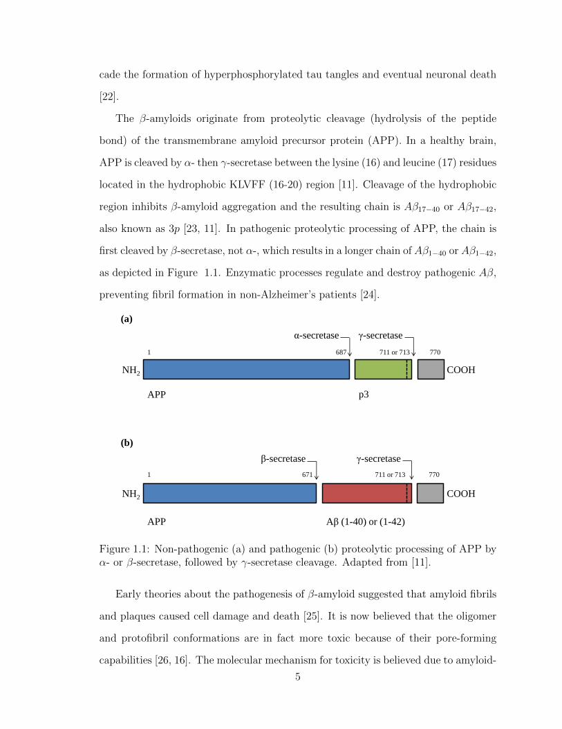
1.1 Non-pathogenic (a) and pathogenic (b) proteolytic processing of APP
by α- or β-secretase, followed by γ-secretase cleavage. . . . . . . . . . 5
1.2 The linear structure of a polypeptide chain showing the links between
carboxyl and amino groups of sequential amino acids. . . . . . . . . . 8
1.3 Amino acids and consequently, the polypeptide backbone consists of
one positively charged and one negatively charged end. This produces
a permanent dipole moment. . . . . . . . . . . . . . . . . . . . . . . . 9
1.4 The two forms of protein secondary structure are shown here: the
α-helix and the β-strand. An atomic model as well as a shorthand
cartoon model for each conformation is depicted. . . . . . . . . . . . . 10
1.5 Hydrophobic tails bury in the interior during micelle formation as hy-
drophilic regions interact with polar solvents. . . . . . . . . . . . . . . 11
1.6 β-strands may stack in parallel or anti-parallel β-sheets. Hydrogen
bonds form between the NH and CO groups of adjacent strands. . . . 12
1.7 Nucleation starts with oligomer formation of β-amyloid fragments.
Monomers then attach longitudinally to the oligomeric nucleus. . . . 14
1.8 Ribbon representation viewed down the fibril axis showing protofila-
ment structure. Each Aβ polypeptide molecule contains two β-strands
(red and blue) that form parallel stacked β-sheets. . . . . . . . . . . . 15
xii
1.9 Representation of the hydration profile for Aβ1−42 shows the three
types of biological water at various regions in and around the pro-
tein. The confinement of water by a protein causes restricted rotations
and other motions of water molecules resulting in attenuated relax-
ation times. The blue portions of the ribbon are hydrophilic and the
red are hydrophobic. The Aβ1−42 structure was obtained from PDB
ID: 1IYT . . . . . . . . . . . . . . . . . . . . . . . . . . . . . . . . . . 17
2.1 Schematic representation of the polarization processes in a broadband
dielectric spectrum for the real and imaginary parts of the permittivity. 27
2.2 Time-dependence of the polarization P of a dielectric material when
an E field is applied. . . . . . . . . . . . . . . . . . . . . . . . . . . . 29
2.3 Schematic representation of the Cole-Cole plot for a Havriliak-Negami
function where β, γ, and ∆ε are the shape parameters of the H-N
function. . . . . . . . . . . . . . . . . . . . . . . . . . . . . . . . . . . 34
2.4 Model of a double-minimum potential (a) in a steady-state and (b) in
the presence of an applied electric field. The application of an electric
field causes a shift in the potentials such that an energy barrier is created. 35
2.5 The fragility of glass forming materials can be visualized diagrammat-
ically by the deviation from Arrhenius-type behavior. . . . . . . . . . 36
2.6 Material dipoles are typically in a random orientation. When placed
inside an electric field, the dipoles align between the capacitive plates. 37
2.7 In dielectric relaxation spectroscopy (DRS), complex impedance is cal-
culated from the ratio of the applied voltage and induced current with
a phase shift. . . . . . . . . . . . . . . . . . . . . . . . . . . . . . . . 38
2.8 A schematic diagram of DRS gain phase measurement. Two probing
voltages are used to compute the complex permittivity. . . . . . . . . 39
xiii
2.9 Block diagram of the Novocontrol Broadband Dielectric/Impedance
Spectrometer apparatus with the Alpha-A analyzer and Quatro
Cryosystem. . . . . . . . . . . . . . . . . . . . . . . . . . . . . . . . . 40
2.10 Cross-section views of the two sample cells used for collecting permit-
tivity data. (a) The BDS 1309 sample cell was used for room tempera-
ture data. The approximate volume is 0.5mL.(b) The BDS 1307 sample
cell was used for low temperature data. The approximate volume is
1.8mL. . . . . . . . . . . . . . . . . . . . . . . . . . . . . . . . . . . . 41
2.11 Fits to the real (ε′) and imaginary (ε′′) part of the dielectric permittiv-
ity using two Havriliak-Negami functions and conductivity. The low
frequency rise in ε′ that lies outside of the fit function is most likely
due to electrode polarization. . . . . . . . . . . . . . . . . . . . . . . 44
2.12 Fits to maximum relaxation frequency, fmax inverse temperature,
1000/T for two relaxation processes. The linear Arrhenius and curved
VFT behaviors are depicted. . . . . . . . . . . . . . . . . . . . . . . . 44
2.13 Amino acid sequences of (a) Aβ1−42 and (b) scrambled Aβ42−1. The
hydrophobic amino acids are shown in red. The sequence found in
native Aβ1−42 possesses a hydrophilic head, hydrophobic tail, and a
hydrophobic region in the middle that causes the β turn in the sec-
ondary structure. . . . . . . . . . . . . . . . . . . . . . . . . . . . . . 45
2.14 Amino acid sequences of (a) human hIAPP22−27 and (b) rat
rIAPP20−29. The hydrophobic amino acids are shown in red. The
arrow points to a proline substitution at amino acid position 25 that
prevents β-sheet formation in rat amylin. . . . . . . . . . . . . . . . . 46
xiv
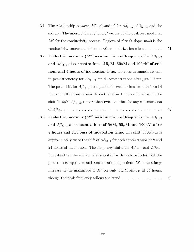
3.1 The relationship between M ′′, ε′, and ε′′ for Aβ1−42, Aβ42−1, and the
solvent. The intersection of ε′ and ε′′ occurs at the peak loss modulus,
M ′′ for the conductivity process. Regions of ε′ with slope, m=0 is the
conductivity process and slope m<0 are polarization effects. . . . . . 51
3.2 Dielectric modulus (M ′′) as a function of frequency for Aβ1−42
and Aβ42−1 at concentrations of 5µM, 50µM and 100µM after 1
hour and 4 hours of incubation time. There is an immediate shift
in peak frequency for Aβ1−42 for all concentrations after just 1 hour.
The peak shift for Aβ42−1 is only a half decade or less for both 1 and 4
hours for all concentrations. Note that after 4 hours of incubation, the
shift for 5µM Aβ1−42 is more than twice the shift for any concentration
of Aβ42−1. . . . . . . . . . . . . . . . . . . . . . . . . . . . . . . . . . 52
3.3 Dielectric modulus (M ′′) as a function of frequency for Aβ1−42
and Aβ42−1 at concentrations of 5µM, 50µM and 100µM after
8 hours and 24 hours of incubation time. The shift for Aβ42−1 is
approximately twice the shift of Aβ42−1 for each concentration at 8 and
24 hours of incubation. The frequency shifts for Aβ1−42 and Aβ42−1
indicates that there is some aggregation with both peptides, but the
process is composition and concentration dependent. We note a large
increase in the magnitude of M ′′ for only 50µM Aβ1−42 at 24 hours,
though the peak frequency follows the trend. . . . . . . . . . . . . . . 53
xv
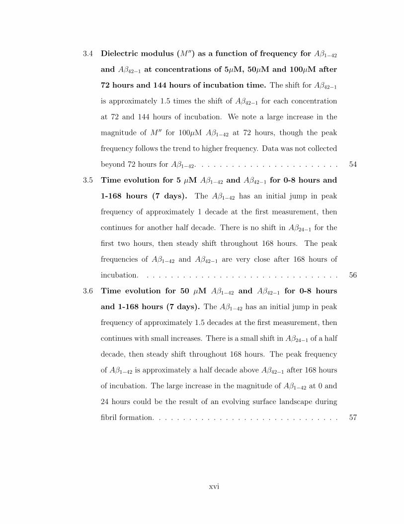
3.4 Dielectric modulus (M ′′) as a function of frequency for Aβ1−42
and Aβ42−1 at concentrations of 5µM, 50µM and 100µM after
72 hours and 144 hours of incubation time. The shift for Aβ42−1
is approximately 1.5 times the shift of Aβ42−1 for each concentration
at 72 and 144 hours of incubation. We note a large increase in the
magnitude of M ′′ for 100µM Aβ1−42 at 72 hours, though the peak
frequency follows the trend to higher frequency. Data was not collected
beyond 72 hours for Aβ1−42. . . . . . . . . . . . . . . . . . . . . . . . 54
3.5 Time evolution for 5 µM Aβ1−42 and Aβ42−1 for 0-8 hours and
1-168 hours (7 days). The Aβ1−42 has an initial jump in peak
frequency of approximately 1 decade at the first measurement, then
continues for another half decade. There is no shift in Aβ24−1 for the
first two hours, then steady shift throughout 168 hours. The peak
frequencies of Aβ1−42 and Aβ42−1 are very close after 168 hours of
incubation. . . . . . . . . . . . . . . . . . . . . . . . . . . . . . . . . 56
3.6 Time evolution for 50 µM Aβ1−42 and Aβ42−1 for 0-8 hours
and 1-168 hours (7 days). The Aβ1−42 has an initial jump in peak
frequency of approximately 1.5 decades at the first measurement, then
continues with small increases. There is a small shift in Aβ24−1 of a half
decade, then steady shift throughout 168 hours. The peak frequency
of Aβ1−42 is approximately a half decade above Aβ42−1 after 168 hours
of incubation. The large increase in the magnitude of Aβ1−42 at 0 and
24 hours could be the result of an evolving surface landscape during
fibril formation. . . . . . . . . . . . . . . . . . . . . . . . . . . . . . . 57
xvi
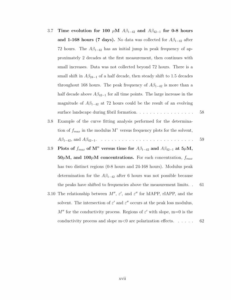
3.7 Time evolution for 100 µM Aβ1−42 and Aβ42−1 for 0-8 hours
and 1-168 hours (7 days). No data was collected for Aβ1−42 after
72 hours. The Aβ1−42 has an initial jump in peak frequency of ap-
proximately 2 decades at the first measurement, then continues with
small increases. Data was not collected beyond 72 hours. There is a
small shift in Aβ24−1 of a half decade, then steady shift to 1.5 decades
throughout 168 hours. The peak frequency of Aβ1−42 is more than a
half decade above Aβ42−1 for all time points. The large increase in the
magnitude of Aβ1−42 at 72 hours could be the result of an evolving
surface landscape during fibril formation. . . . . . . . . . . . . . . . . 58
3.8 Example of the curve fitting analysis performed for the determina-
tion of fmax in the modulus M” versus frequency plots for the solvent,
Aβ1−42, and Aβ42−1. . . . . . . . . . . . . . . . . . . . . . . . . . . . 59
3.9 Plots of fmax of M” versus time for Aβ1−42 and Aβ42−1 at 5µM,
50µM, and 100µM concentrations. For each concentration, fmax
has two distinct regions (0-8 hours and 24-168 hours). Modulus peak
determination for the Aβ1−42 after 6 hours was not possible because
the peaks have shifted to frequencies above the measurement limits. . 61
3.10 The relationship between M ′′, ε′, and ε′′ for hIAPP, rIAPP, and the
solvent. The intersection of ε′ and ε′′ occurs at the peak loss modulus,
M ′′ for the conductivity process. Regions of ε′ with slope, m=0 is the
conductivity process and slope m<0 are polarization effects. . . . . . 62
xvii
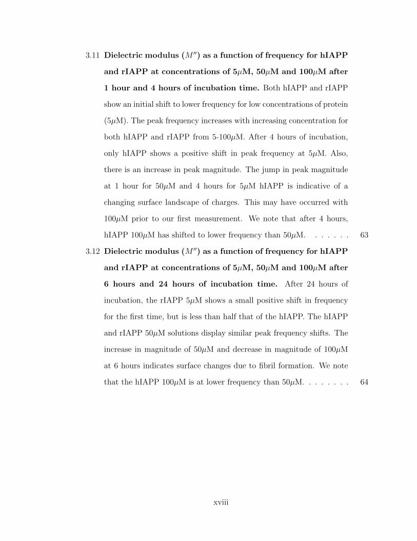
3.11 Dielectric modulus (M ′′) as a function of frequency for hIAPP
and rIAPP at concentrations of 5µM, 50µM and 100µM after
1 hour and 4 hours of incubation time. Both hIAPP and rIAPP
show an initial shift to lower frequency for low concentrations of protein
(5µM). The peak frequency increases with increasing concentration for
both hIAPP and rIAPP from 5-100µM. After 4 hours of incubation,
only hIAPP shows a positive shift in peak frequency at 5µM. Also,
there is an increase in peak magnitude. The jump in peak magnitude
at 1 hour for 50µM and 4 hours for 5µM hIAPP is indicative of a
changing surface landscape of charges. This may have occurred with
100µM prior to our first measurement. We note that after 4 hours,
hIAPP 100µM has shifted to lower frequency than 50µM. . . . . . . 63
3.12 Dielectric modulus (M ′′) as a function of frequency for hIAPP
and rIAPP at concentrations of 5µM, 50µM and 100µM after
6 hours and 24 hours of incubation time. After 24 hours of
incubation, the rIAPP 5µM shows a small positive shift in frequency
for the first time, but is less than half that of the hIAPP. The hIAPP
and rIAPP 50µM solutions display similar peak frequency shifts. The
increase in magnitude of 50µM and decrease in magnitude of 100µM
at 6 hours indicates surface changes due to fibril formation. We note
that the hIAPP 100µM is at lower frequency than 50µM. . . . . . . . 64
xviii
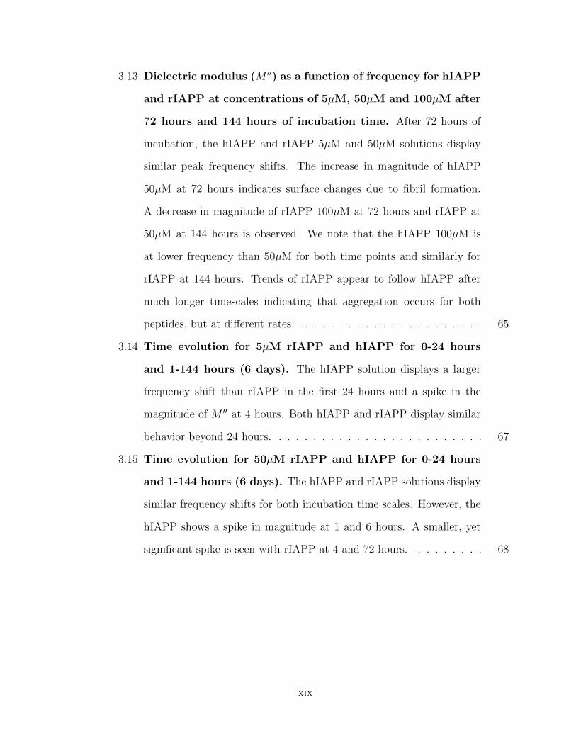
3.13 Dielectric modulus (M ′′) as a function of frequency for hIAPP
and rIAPP at concentrations of 5µM, 50µM and 100µM after
72 hours and 144 hours of incubation time. After 72 hours of
incubation, the hIAPP and rIAPP 5µM and 50µM solutions display
similar peak frequency shifts. The increase in magnitude of hIAPP
50µM at 72 hours indicates surface changes due to fibril formation.
A decrease in magnitude of rIAPP 100µM at 72 hours and rIAPP at
50µM at 144 hours is observed. We note that the hIAPP 100µM is
at lower frequency than 50µM for both time points and similarly for
rIAPP at 144 hours. Trends of rIAPP appear to follow hIAPP after
much longer timescales indicating that aggregation occurs for both
peptides, but at different rates. . . . . . . . . . . . . . . . . . . . . . 65
3.14 Time evolution for 5µM rIAPP and hIAPP for 0-24 hours
and 1-144 hours (6 days). The hIAPP solution displays a larger
frequency shift than rIAPP in the first 24 hours and a spike in the
magnitude of M ′′ at 4 hours. Both hIAPP and rIAPP display similar
behavior beyond 24 hours. . . . . . . . . . . . . . . . . . . . . . . . . 67
3.15 Time evolution for 50µM rIAPP and hIAPP for 0-24 hours
and 1-144 hours (6 days). The hIAPP and rIAPP solutions display
similar frequency shifts for both incubation time scales. However, the
hIAPP shows a spike in magnitude at 1 and 6 hours. A smaller, yet
significant spike is seen with rIAPP at 4 and 72 hours. . . . . . . . . 68
xix
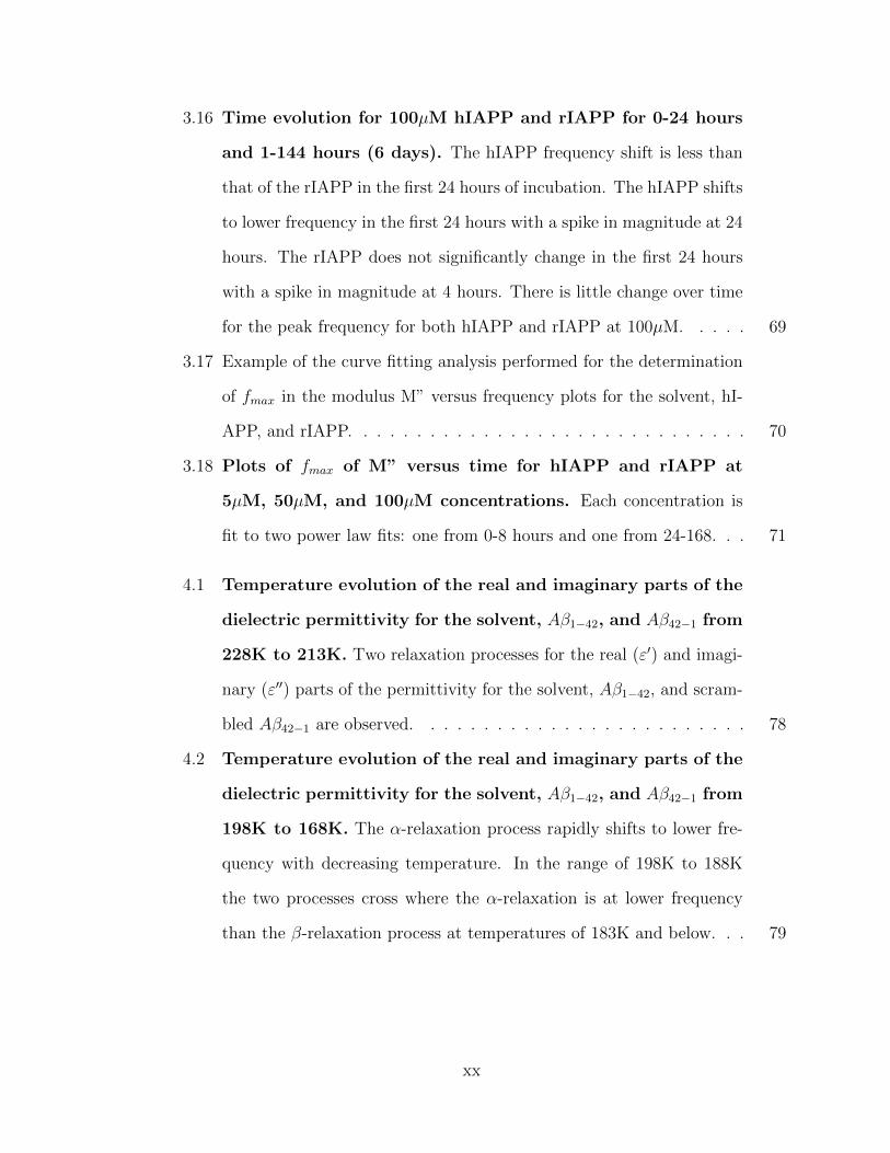
3.16 Time evolution for 100µM hIAPP and rIAPP for 0-24 hours
and 1-144 hours (6 days). The hIAPP frequency shift is less than
that of the rIAPP in the first 24 hours of incubation. The hIAPP shifts
to lower frequency in the first 24 hours with a spike in magnitude at 24
hours. The rIAPP does not significantly change in the first 24 hours
with a spike in magnitude at 4 hours. There is little change over time
for the peak frequency for both hIAPP and rIAPP at 100µM. . . . . 69
3.17 Example of the curve fitting analysis performed for the determination
of fmax in the modulus M” versus frequency plots for the solvent, hI-
APP, and rIAPP. . . . . . . . . . . . . . . . . . . . . . . . . . . . . . 70
3.18 Plots of fmax of M” versus time for hIAPP and rIAPP at
5µM, 50µM, and 100µM concentrations. Each concentration is
fit to two power law fits: one from 0-8 hours and one from 24-168. . . 71
4.1 Temperature evolution of the real and imaginary parts of the
dielectric permittivity for the solvent, Aβ1−42, and Aβ42−1 from
228K to 213K. Two relaxation processes for the real (ε′) and imagi-
nary (ε′′) parts of the permittivity for the solvent, Aβ1−42, and scram-
bled Aβ42−1 are observed. . . . . . . . . . . . . . . . . . . . . . . . . 78
4.2 Temperature evolution of the real and imaginary parts of the
dielectric permittivity for the solvent, Aβ1−42, and Aβ42−1 from
198K to 168K. The α-relaxation process rapidly shifts to lower fre-
quency with decreasing temperature. In the range of 198K to 188K
the two processes cross where the α-relaxation is at lower frequency
than the β-relaxation process at temperatures of 183K and below. . . 79
xx
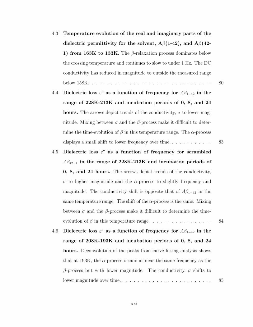
4.3 Temperature evolution of the real and imaginary parts of the
dielectric permittivity for the solvent, Aβ(1-42), and Aβ(42-
1) from 163K to 133K. The β-relaxation process dominates below
the crossing temperature and continues to slow to under 1 Hz. The DC
conductivity has reduced in magnitude to outside the measured range
below 158K. . . . . . . . . . . . . . . . . . . . . . . . . . . . . . . . . 80
4.4 Dielectric loss ε′′ as a function of frequency for Aβ1−42 in the
range of 228K-213K and incubation periods of 0, 8, and 24
hours. The arrows depict trends of the conductivity, σ to lower mag-
nitude. Mixing between σ and the β-process make it difficult to deter-
mine the time-evolution of β in this temperature range. The α-process
displays a small shift to lower frequency over time. . . . . . . . . . . . 83
4.5 Dielectric loss ε′′ as a function of frequency for scrambled
Aβ42−1 in the range of 228K-213K and incubation periods of
0, 8, and 24 hours. The arrows depict trends of the conductivity,
σ to higher magnitude and the α-process to slightly frequency and
magnitude. The conductivity shift is opposite that of Aβ1−42 in the
same temperature range. The shift of the α-process is the same. Mixing
between σ and the β-process make it difficult to determine the time-
evolution of β in this temperature range. . . . . . . . . . . . . . . . . 84
4.6 Dielectric loss ε′′ as a function of frequency for Aβ1−42 in the
range of 208K-193K and incubation periods of 0, 8, and 24
hours. Deconvolution of the peaks from curve fitting analysis shows
that at 193K, the α-process occurs at near the same frequency as the
β-process but with lower magnitude. The conductivity, σ shifts to
lower magnitude over time. . . . . . . . . . . . . . . . . . . . . . . . . 85
xxi
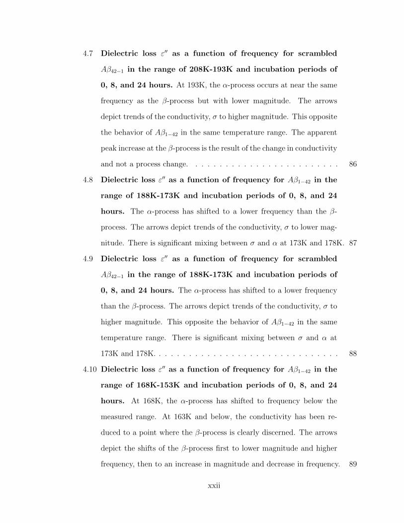
4.7 Dielectric loss ε′′ as a function of frequency for scrambled
Aβ42−1 in the range of 208K-193K and incubation periods of
0, 8, and 24 hours. At 193K, the α-process occurs at near the same
frequency as the β-process but with lower magnitude. The arrows
depict trends of the conductivity, σ to higher magnitude. This opposite
the behavior of Aβ1−42 in the same temperature range. The apparent
peak increase at the β-process is the result of the change in conductivity
and not a process change. . . . . . . . . . . . . . . . . . . . . . . . . 86
4.8 Dielectric loss ε′′ as a function of frequency for Aβ1−42 in the
range of 188K-173K and incubation periods of 0, 8, and 24
hours. The α-process has shifted to a lower frequency than the β-
process. The arrows depict trends of the conductivity, σ to lower mag-
nitude. There is significant mixing between σ and α at 173K and 178K. 87
4.9 Dielectric loss ε′′ as a function of frequency for scrambled
Aβ42−1 in the range of 188K-173K and incubation periods of
0, 8, and 24 hours. The α-process has shifted to a lower frequency
than the β-process. The arrows depict trends of the conductivity, σ to
higher magnitude. This opposite the behavior of Aβ1−42 in the same
temperature range. There is significant mixing between σ and α at
173K and 178K. . . . . . . . . . . . . . . . . . . . . . . . . . . . . . . 88
4.10 Dielectric loss ε′′ as a function of frequency for Aβ1−42 in the
range of 168K-153K and incubation periods of 0, 8, and 24
hours. At 168K, the α-process has shifted to frequency below the
measured range. At 163K and below, the conductivity has been re-
duced to a point where the β-process is clearly discerned. The arrows
depict the shifts of the β-process first to lower magnitude and higher
frequency, then to an increase in magnitude and decrease in frequency. 89
xxii
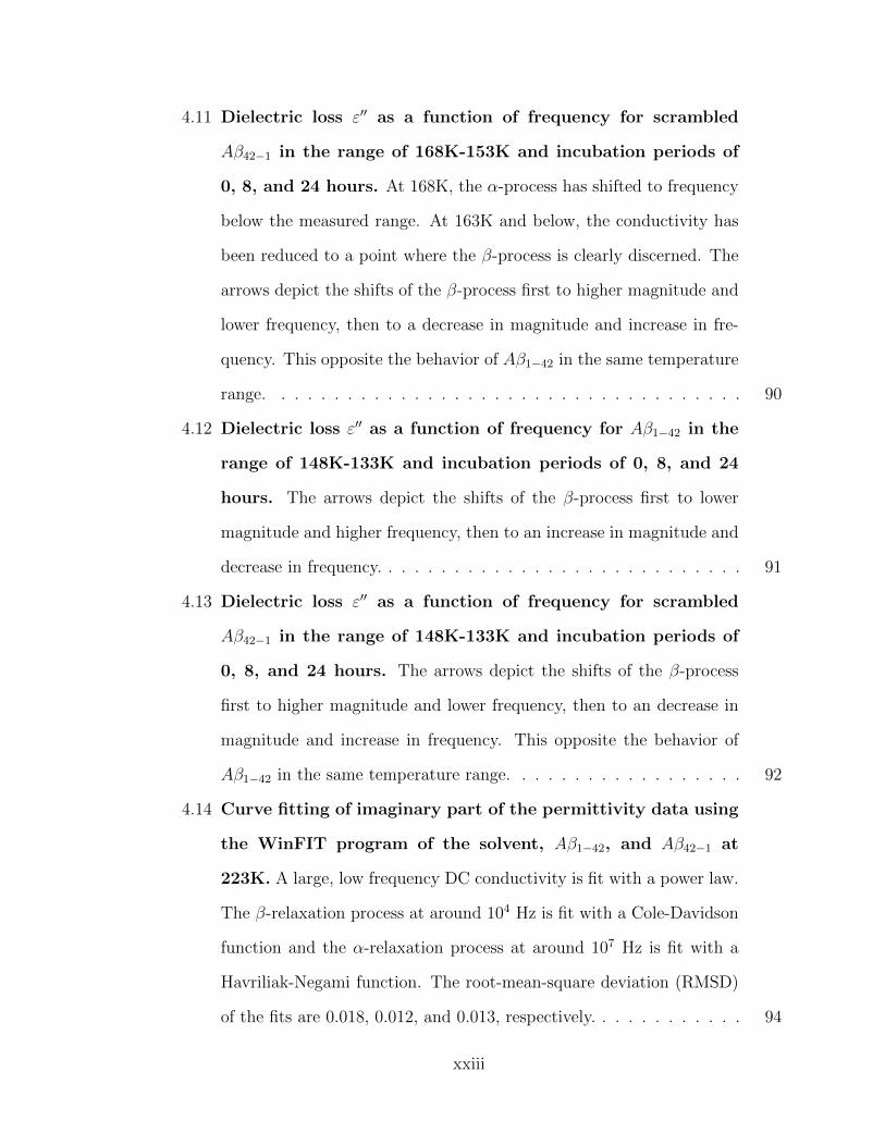
4.11 Dielectric loss ε′′ as a function of frequency for scrambled
Aβ42−1 in the range of 168K-153K and incubation periods of
0, 8, and 24 hours. At 168K, the α-process has shifted to frequency
below the measured range. At 163K and below, the conductivity has
been reduced to a point where the β-process is clearly discerned. The
arrows depict the shifts of the β-process first to higher magnitude and
lower frequency, then to a decrease in magnitude and increase in fre-
quency. This opposite the behavior of Aβ1−42 in the same temperature
range. . . . . . . . . . . . . . . . . . . . . . . . . . . . . . . . . . . . 90
4.12 Dielectric loss ε′′ as a function of frequency for Aβ1−42 in the
range of 148K-133K and incubation periods of 0, 8, and 24
hours. The arrows depict the shifts of the β-process first to lower
magnitude and higher frequency, then to an increase in magnitude and
decrease in frequency. . . . . . . . . . . . . . . . . . . . . . . . . . . . 91
4.13 Dielectric loss ε′′ as a function of frequency for scrambled
Aβ42−1 in the range of 148K-133K and incubation periods of
0, 8, and 24 hours. The arrows depict the shifts of the β-process
first to higher magnitude and lower frequency, then to an decrease in
magnitude and increase in frequency. This opposite the behavior of
Aβ1−42 in the same temperature range. . . . . . . . . . . . . . . . . . 92
4.14 Curve fitting of imaginary part of the permittivity data using
the WinFIT program of the solvent, Aβ1−42, and Aβ42−1 at
223K. A large, low frequency DC conductivity is fit with a power law.
The β-relaxation process at around 104 Hz is fit with a Cole-Davidson
function and the α-relaxation process at around 107 Hz is fit with a
Havriliak-Negami function. The root-mean-square deviation (RMSD)
of the fits are 0.018, 0.012, and 0.013, respectively. . . . . . . . . . . . 94
xxiii

4.15 Curve fitting of imaginary part of the permittivity data using
the WinFIT program of the solvent, Aβ1−42, and Aβ42−1 at
208K. A large, low frequency DC conductivity is fit with a power law.
The β-relaxation process at around 103 Hz is fit with a Cole-Davidson
function and the α-relaxation process at around 105 Hz is fit with a
Havriliak-Negami function. The RMSD of the fits are 0.045, 0.009, and
0.013, respectively. . . . . . . . . . . . . . . . . . . . . . . . . . . . . 95
4.16 Curve fitting of imaginary part of the permittivity data using
the WinFIT program of the solvent, Aβ1−42, and Aβ42−1 at
188K. A large, low frequency DC conductivity is fit with a power law.
The β-relaxation process at around 103 Hz is fit with a Cole-Davidson
function and the α-relaxation process at around 101 Hz is fit with a
Havriliak-Negami function. Here, the α process has crossed over to
slower than β relaxation times. The RMSD of the fits are 0.008, 0.011,
and 0.013, respectively. . . . . . . . . . . . . . . . . . . . . . . . . . . 96
4.17 Curve fitting of the imaginary part of the permittivity data
using the WinFIT program of the solvent, Aβ1−42, and Aβ42−1
at 133K. A small, very low frequency DC conductivity is fit with a
power law. The β-relaxation process at around 1 Hz is fit with a Cole-
Davidson function and the α-relaxation process is not observed. The
RMSD of the fits are 0.092, 0.123, and 0.082, respectively. . . . . . . 97
4.18 Arrhenius plots of fmax versus inverse temperature for Aβ1−42
over time. The α-relaxation process follows a VFT behavior whereas
the β-relaxation process follows an Arrhenius, or linear behavior. The
α-process departs from the VFT curvature at low temperature. . . . . 99
xxiv

4.19 Arrhenius plots of fmax versus inverse temperature for scram-
bled Aβ42−1 over time. The α-relaxation process follows a VFT
behavior whereas the β-relaxation process follows an Arrhenius, or lin-
ear behavior. The α-process departs from the VFT curvature at low
temperature. . . . . . . . . . . . . . . . . . . . . . . . . . . . . . . . . 100
4.20 Dielectric strength, ∆ε of the β-relaxation for Aβ1−42 and
Aβ42−1 versus inverse temperature. The dielectric strength for the
Aβ1−42 solution first increases, then deceases to values less than the
solvent. The dielectric strength of Aβ42−1 continued to increase over
time. The decrease in dielectric strength indicates that the Aβ1−42
displays an anti-parallel β-sheet conformation. . . . . . . . . . . . . . 102
4.21 Temperature evolution of the real and imaginary parts of the
dielectric permittivity for the solvent, hIAPP, and rIAPP
from 228K to 203K. Two relaxation processes for the real (ε′) and
imaginary (ε′′) parts of the permittivity for the solvent, hIAPP, and
rIAPP are observed. . . . . . . . . . . . . . . . . . . . . . . . . . . . 103
4.22 Temperature evolution of the real and imaginary parts of the
dielectric permittivity for the solvent, hIAPP, and rIAPP
from 198K to 168K. The α-relaxation process rapidly shifts to lower
frequency with decreasing temperature. In the range of 198K to 188K
the two processes cross to where the α-relaxation is at lower frequency
than the β-relaxation process at temperatures of 183K and below. . . 104
xxv
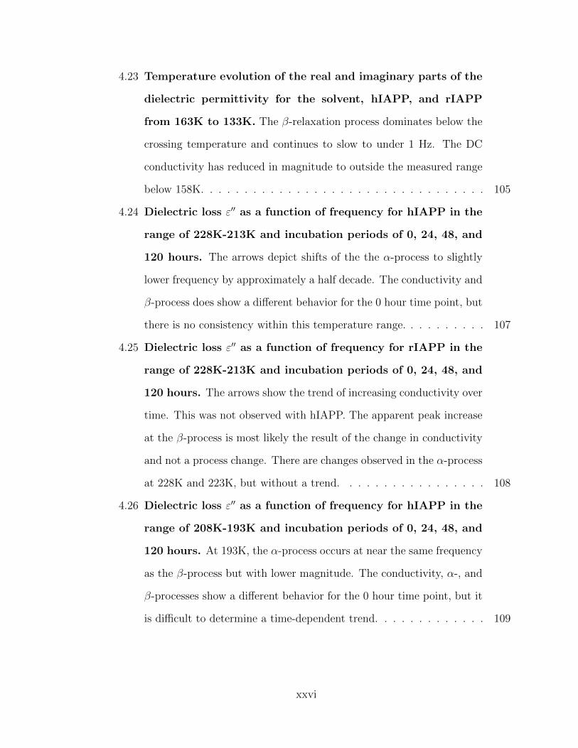
4.23 Temperature evolution of the real and imaginary parts of the
dielectric permittivity for the solvent, hIAPP, and rIAPP
from 163K to 133K. The β-relaxation process dominates below the
crossing temperature and continues to slow to under 1 Hz. The DC
conductivity has reduced in magnitude to outside the measured range
below 158K. . . . . . . . . . . . . . . . . . . . . . . . . . . . . . . . . 105
4.24 Dielectric loss ε′′ as a function of frequency for hIAPP in the
range of 228K-213K and incubation periods of 0, 24, 48, and
120 hours. The arrows depict shifts of the the α-process to slightly
lower frequency by approximately a half decade. The conductivity and
β-process does show a different behavior for the 0 hour time point, but
there is no consistency within this temperature range. . . . . . . . . . 107
4.25 Dielectric loss ε′′ as a function of frequency for rIAPP in the
range of 228K-213K and incubation periods of 0, 24, 48, and
120 hours. The arrows show the trend of increasing conductivity over
time. This was not observed with hIAPP. The apparent peak increase
at the β-process is most likely the result of the change in conductivity
and not a process change. There are changes observed in the α-process
at 228K and 223K, but without a trend. . . . . . . . . . . . . . . . . 108
4.26 Dielectric loss ε′′ as a function of frequency for hIAPP in the
range of 208K-193K and incubation periods of 0, 24, 48, and
120 hours. At 193K, the α-process occurs at near the same frequency
as the β-process but with lower magnitude. The conductivity, α-, and
β-processes show a different behavior for the 0 hour time point, but it
is difficult to determine a time-dependent trend. . . . . . . . . . . . . 109
xxvi
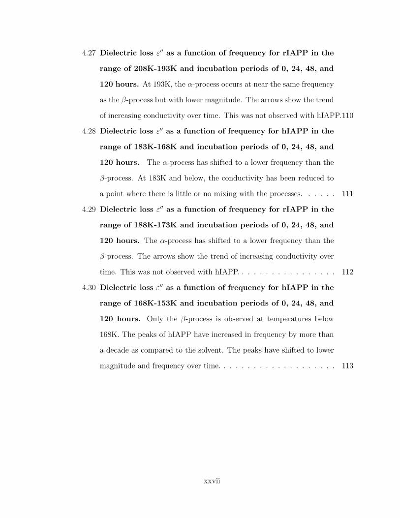
4.27 Dielectric loss ε′′ as a function of frequency for rIAPP in the
range of 208K-193K and incubation periods of 0, 24, 48, and
120 hours. At 193K, the α-process occurs at near the same frequency
as the β-process but with lower magnitude. The arrows show the trend
of increasing conductivity over time. This was not observed with hIAPP.110
4.28 Dielectric loss ε′′ as a function of frequency for hIAPP in the
range of 183K-168K and incubation periods of 0, 24, 48, and
120 hours. The α-process has shifted to a lower frequency than the
β-process. At 183K and below, the conductivity has been reduced to
a point where there is little or no mixing with the processes. . . . . . 111
4.29 Dielectric loss ε′′ as a function of frequency for rIAPP in the
range of 188K-173K and incubation periods of 0, 24, 48, and
120 hours. The α-process has shifted to a lower frequency than the
β-process. The arrows show the trend of increasing conductivity over
time. This was not observed with hIAPP. . . . . . . . . . . . . . . . . 112
4.30 Dielectric loss ε′′ as a function of frequency for hIAPP in the
range of 168K-153K and incubation periods of 0, 24, 48, and
120 hours. Only the β-process is observed at temperatures below
168K. The peaks of hIAPP have increased in frequency by more than
a decade as compared to the solvent. The peaks have shifted to lower
magnitude and frequency over time. . . . . . . . . . . . . . . . . . . . 113
xxvii

4.31 Dielectric loss ε′′ as a function of frequency for rIAPP in the
range of 168K-153K and incubation periods of 0, 24, 48, and
120 hours. Only the β-process is observed at temperatures below
158K. The arrows show that the conductivity increases and the β-
process peaks shift to higher magnitude over time. This opposite the
behavior of hIAPP in the same temperature range. There is no increase
in frequency at t = 0hr, where hIAPP displayed a decade shift. The
shift in peak position at 168K and 163K may be due to conductivity. 114
4.32 Dielectric loss ε′′ as a function of frequency for hIAPP in the
range of 148K-133K and incubation periods of 0, 24, 48, and
120 hours. The arrows depict that the β-process of hIAPP shifts to
lower frequency and lower magnitude over time. . . . . . . . . . . . . 115
4.33 Dielectric loss ε′′ as a function of frequency for rIAPP in the
range of 148K-133K and incubation periods of 0, 24, 48, and
120 hours. The arrows depict that the β-process of rIAPP shifts to
lower frequency and higher magnitude over time. This opposite the
behavior of hIAPP in the same temperature range. . . . . . . . . . . 116
4.34 Curve fitting of imaginary part of the permittivity data using
the WinFIT program of the solvent, hIAPP, and rIAPP at
223K. A large, low frequency DC conductivity is fit with a power
law. The α-relaxation process at around 107 Hz is fit with a Havriliak-
Negami function and the β-relaxation function is not observed. The
RMSD of the fits are 0.015, 0.005, and 0.016, respectively. . . . . . . 118
xxviii
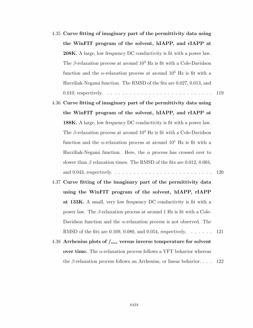
4.35 Curve fitting of imaginary part of the permittivity data using
the WinFIT program of the solvent, hIAPP, and rIAPP at
208K. A large, low frequency DC conductivity is fit with a power law.
The β-relaxation process at around 103 Hz is fit with a Cole-Davidson
function and the α-relaxation process at around 105 Hz is fit with a
Havriliak-Negami function. The RMSD of the fits are 0.027, 0.013, and
0.010, respectively. . . . . . . . . . . . . . . . . . . . . . . . . . . . . 119
4.36 Curve fitting of imaginary part of the permittivity data using
the WinFIT program of the solvent, hIAPP, and rIAPP at
188K. A large, low frequency DC conductivity is fit with a power law.
The β-relaxation process at around 103 Hz is fit with a Cole-Davidson
function and the α-relaxation process at around 101 Hz is fit with a
Havriliak-Negami function. Here, the α process has crossed over to
slower than β relaxation times. The RMSD of the fits are 0.012, 0.004,
and 0.043, respectively. . . . . . . . . . . . . . . . . . . . . . . . . . . 120
4.37 Curve fitting of the imaginary part of the permittivity data
using the WinFIT program of the solvent, hIAPP, rIAPP
at 133K. A small, very low frequency DC conductivity is fit with a
power law. The β-relaxation process at around 1 Hz is fit with a Cole-
Davidson function and the α-relaxation process is not observed. The
RMSD of the fits are 0.169, 0.080, and 0.054, respectively. . . . . . . 121
4.38 Arrhenius plots of fmax versus inverse temperature for solvent
over time. The α-relaxation process follows a VFT behavior whereas
the β-relaxation process follows an Arrhenius, or linear behavior. . . . 122
xxix

4.39 Arrhenius plots of fmax versus inverse temperature for hIAPP
from 0-120 hours. The α-relaxation process follows a VFT behavior
whereas the β-relaxation process follows an Arrhenius, or linear behav-
ior. The α-process departs from the VFT curvature at low temperature.123
4.40 Arrhenius plots of fmax versus inverse temperature for rIAPP
from 0-120 hours. The α-relaxation process follows a VFT behavior
whereas the β-relaxation process follows an Arrhenius, or linear behav-
ior. The α-process departs from the VFT curvature at low temperature.124
4.41 Dielectric strength, ∆ε of the β-relaxation for hIAPP and
rIAPP versus inverse temperature. The dielectric strength for
the hIAPP solution first increases, then deceases to values less than
the solvent. The dielectric strength of rIAPP continued to increase
over time. This indicates a mixed grouping of parallel and anti-parallel
β-sheets in hIAPP and random-coil aggregation in rIAPP. . . . . . . 126
4.42 Plots of the β-relaxation peak shift at 143K for Aβ1−42/Aβ42−1 and
hIAPP/rIAPP as compared to the solvent. . . . . . . . . . . . . . . . 128
4.43 Arrhenius plots of fmax versus inverse temperature for pure
glycerol and glycerol-water mixtures of approximately 50-50%
by weight [63, 158, 142, 78]. The glycerol-water mixtures display
both α- and β-relaxation processes. Only the α process appears in
pure glycerol. . . . . . . . . . . . . . . . . . . . . . . . . . . . . . . . 129
5.1 Temperature evolution of the real and imaginary parts of the
dielectric permittivity for the solvent, Aβ1−42, and Aβ42−1 from
223K to 198K. Two relaxation processes for the real (ε′) and imagi-
nary (ε′′) parts of the permittivity for the solvent, Aβ1−42, and scram-
bled Aβ42−1 are observed. . . . . . . . . . . . . . . . . . . . . . . . . 134
xxx

5.2 Temperature evolution of the real and imaginary parts of the
dielectric permittivity for the solvent,Aβ1−42, and Aβ42−1 from
193K to 168K. The α-relaxation process rapidly shifts to lower fre-
quency with decreasing temperature. In the range of 193K to 188K
the two processes cross where the α-relaxation is at lower frequency
than the β-relaxation process at temperatures of 183K and below. . . 135
5.3 Temperature evolution of the real and imaginary parts of the
dielectric permittivity for the solvent, Aβ1−42, and Aβ42−1 from
163K to 133K. The β-relaxation process dominates below the cross-
ing temperature and continues to slow to under 1 Hz. The DC conduc-
tivity has reduced in magnitude to outside the measured range below
158K. . . . . . . . . . . . . . . . . . . . . . . . . . . . . . . . . . . . 136
5.4 Dielectric loss ε′′ as a function of frequency for Aβ1−42 in
the range of 223K-208K and incubation periods of 0, 8, and
24 hours. At temperatures above 208K, the β-relaxation process
is masked by the conductivity, σ. The arrows depict a decrease in
magnitude of ε′′, due to the decrease in σ over time. The spectra
shows a shift towards higher frequency at 223K, but does not appear
to follow a trend. . . . . . . . . . . . . . . . . . . . . . . . . . . . . . 138
5.5 Dielectric loss ε′′ as a function of frequency for scrambled
Aβ42−1 in the range of 223K-208K and incubation periods of
0, 8, and 24 hours. At temperatures above 208K, the β-relaxation
process is masked by the conductivity, σ. The arrows depict a small
decrease in magnitude of ε′′, due to the decrease in σ over time. As
with Aβ1−42, the spectra shows a shift towards higher frequency at
223K, but does not appear to follow a trend. . . . . . . . . . . . . . . 139
xxxi
5.6 Dielectric loss ε′′ as a function of frequency for Aβ1−42 in the
range of 203K-188K and incubation periods of 0, 8, and 24
hours. At 193K, the α-process occurs at near the same frequency as
the β-process but with lower magnitude. The arrows show a shift in
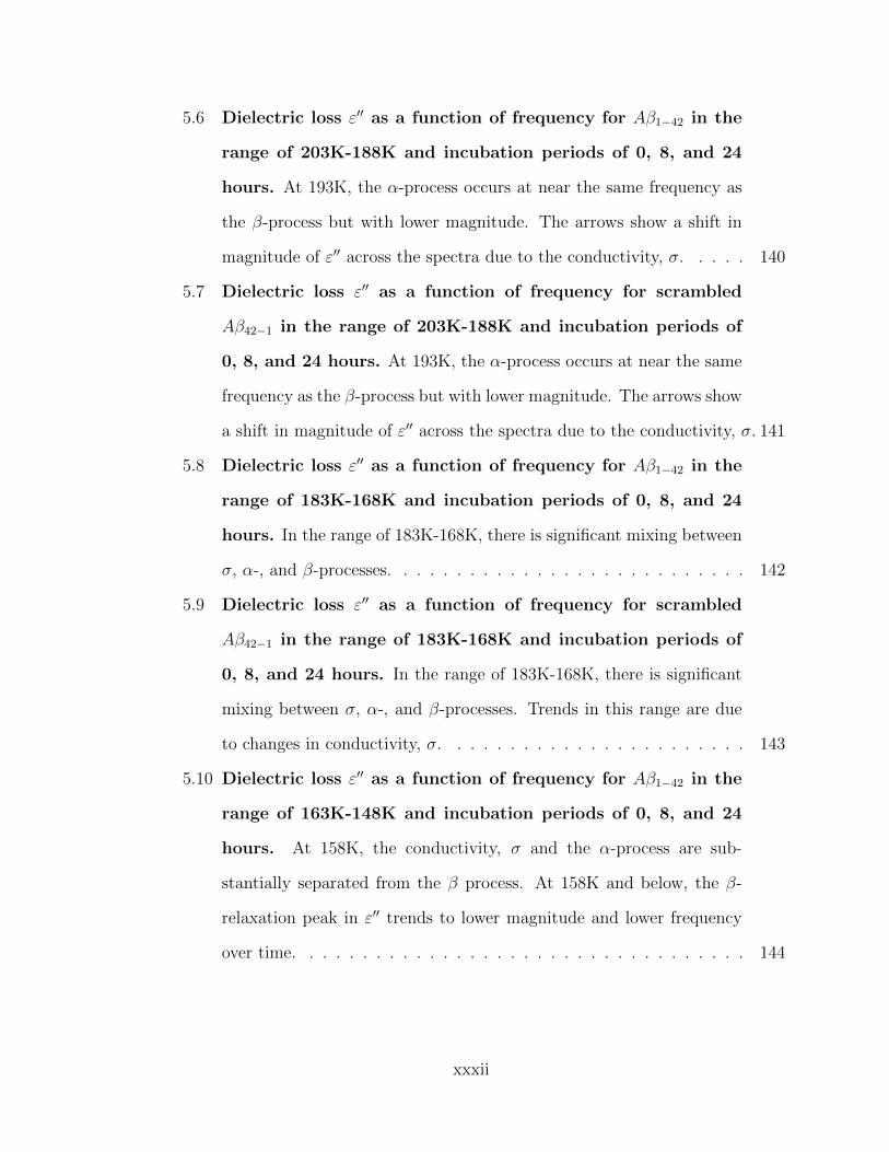
magnitude of ε′′ across the spectra due to the conductivity, σ. . . . . 140
5.7 Dielectric loss ε′′ as a function of frequency for scrambled
Aβ42−1 in the range of 203K-188K and incubation periods of
0, 8, and 24 hours. At 193K, the α-process occurs at near the same
frequency as the β-process but with lower magnitude. The arrows show
a shift in magnitude of ε′′ across the spectra due to the conductivity, σ. 141
5.8 Dielectric loss ε′′ as a function of frequency for Aβ1−42 in the
range of 183K-168K and incubation periods of 0, 8, and 24
hours. In the range of 183K-168K, there is significant mixing between
σ, α-, and β-processes. . . . . . . . . . . . . . . . . . . . . . . . . . . 142
5.9 Dielectric loss ε′′ as a function of frequency for scrambled
Aβ42−1 in the range of 183K-168K and incubation periods of
0, 8, and 24 hours. In the range of 183K-168K, there is significant
mixing between σ, α-, and β-processes. Trends in this range are due
to changes in conductivity, σ. . . . . . . . . . . . . . . . . . . . . . . 143
5.10 Dielectric loss ε′′ as a function of frequency for Aβ1−42 in the
range of 163K-148K and incubation periods of 0, 8, and 24
hours. At 158K, the conductivity, σ and the α-process are sub-
stantially separated from the β process. At 158K and below, the β-
relaxation peak in ε′′ trends to lower magnitude and lower frequency
over time. . . . . . . . . . . . . . . . . . . . . . . . . . . . . . . . . . 144
xxxii

5.11 Dielectric loss ε′′ as a function of frequency for scrambled
Aβ42−1 in the range of 163K-148K and incubation periods of
0, 8, and 24 hours. At 163K, the conductivity, σ and the α-process
are substantially separated from the β process. At 158K and below, the
β-relaxation peak in ε′′ trends to lower magnitude but unlike Aβ1−42,
the peak shifts towards higher frequency over time. . . . . . . . . . . 145
5.12 Dielectric loss ε′′ as a function of frequency for Aβ1−42 in the
range of 143K-133K and incubation periods of 0, 8, and 24
hours. The β-relaxation peak in ε′′ trends to lower magnitude and
lower frequency over time. . . . . . . . . . . . . . . . . . . . . . . . . 146
5.13 Dielectric loss ε′′ as a function of frequency for scrambled
Aβ42−1 in the range of 143K-133K and incubation periods of
0, 8, and 24 hours. The β-relaxation peak in ε′′ trends to lower
magnitude but unlike Aβ1−42, the peak shifts towards higher frequency
over time. . . . . . . . . . . . . . . . . . . . . . . . . . . . . . . . . . 147
5.14 Curve fitting of imaginary part of the permittivity data using
the WinFIT program of the solvent, Aβ1−42, and Aβ42−1 at
223K. A large, low frequency DC conductivity is fit with a power
law. The α-relaxation process at around 107 Hz is fit with a Havriliak-
Negami function. The β-relaxation function is not observed. The
root-mean-square deviation (RMSD) of the fits are 0.015, 0.030, and
0.088, respectively. . . . . . . . . . . . . . . . . . . . . . . . . . . . . 149
xxxiii
5.15 Curve fitting of imaginary part of the permittivity data using
the WinFIT program of the solvent, Aβ1−42, and Aβ42−1 at
208K. A large, low frequency DC conductivity is fit with a power law.
The β-relaxation process at around 103 Hz is fit with a Cole-Davidson
function and the α-relaxation process at around 105 Hz is fit with a
Havriliak-Negami function. The RMSD of the fits are 0.018, 0.005, and
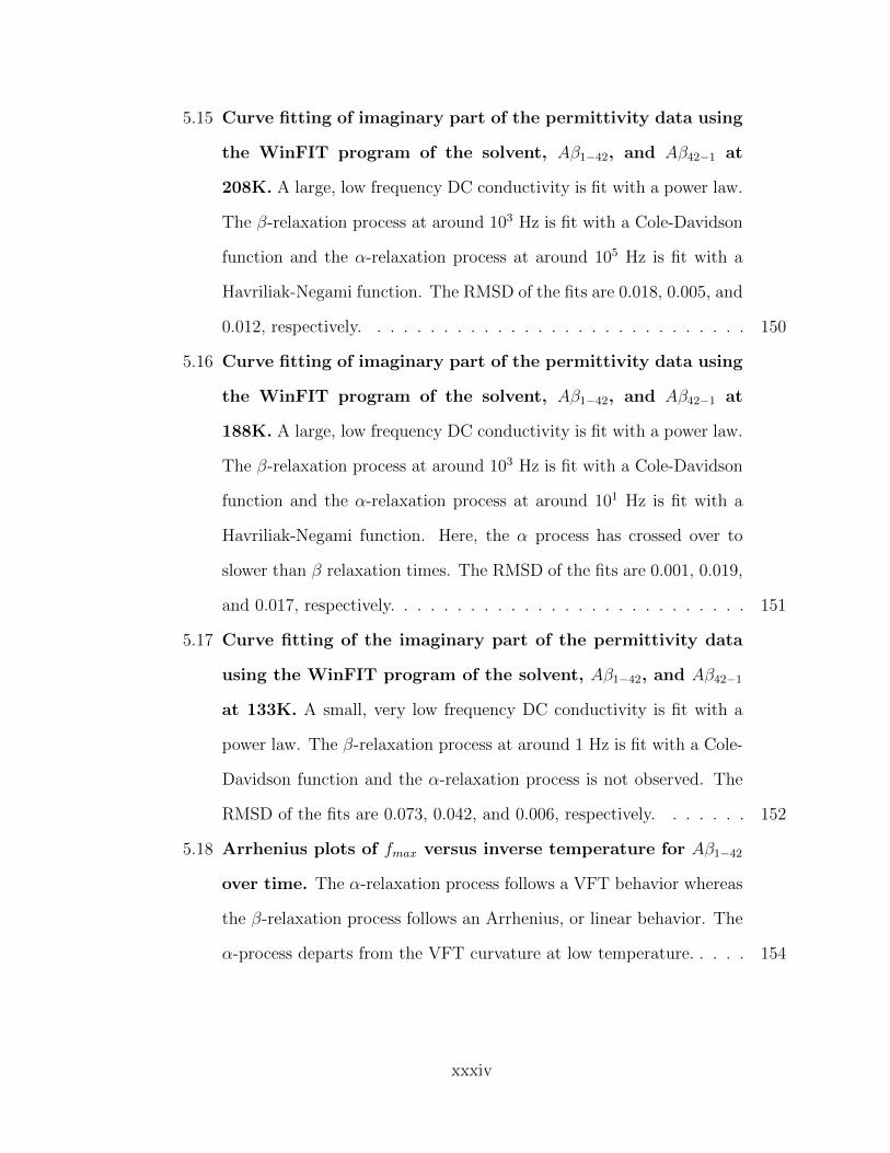
0.012, respectively. . . . . . . . . . . . . . . . . . . . . . . . . . . . . 150
5.16 Curve fitting of imaginary part of the permittivity data using
the WinFIT program of the solvent, Aβ1−42, and Aβ42−1 at
188K. A large, low frequency DC conductivity is fit with a power law.
The β-relaxation process at around 103 Hz is fit with a Cole-Davidson
function and the α-relaxation process at around 101 Hz is fit with a
Havriliak-Negami function. Here, the α process has crossed over to
slower than β relaxation times. The RMSD of the fits are 0.001, 0.019,
and 0.017, respectively. . . . . . . . . . . . . . . . . . . . . . . . . . . 151
5.17 Curve fitting of the imaginary part of the permittivity data
using the WinFIT program of the solvent, Aβ1−42, and Aβ42−1
at 133K. A small, very low frequency DC conductivity is fit with a
power law. The β-relaxation process at around 1 Hz is fit with a Cole-
Davidson function and the α-relaxation process is not observed. The
RMSD of the fits are 0.073, 0.042, and 0.006, respectively. . . . . . . 152
5.18 Arrhenius plots of fmax versus inverse temperature for Aβ1−42
over time. The α-relaxation process follows a VFT behavior whereas
the β-relaxation process follows an Arrhenius, or linear behavior. The
α-process departs from the VFT curvature at low temperature. . . . . 154
xxxiv
5.19 Arrhenius plots of fmax versus inverse temperature for scram-
bled Aβ42−1 over time. The α-relaxation process follows a VFT
behavior whereas the β-relaxation process follows an Arrhenius, or lin-
ear behavior. The α-process departs from the VFT curvature at low
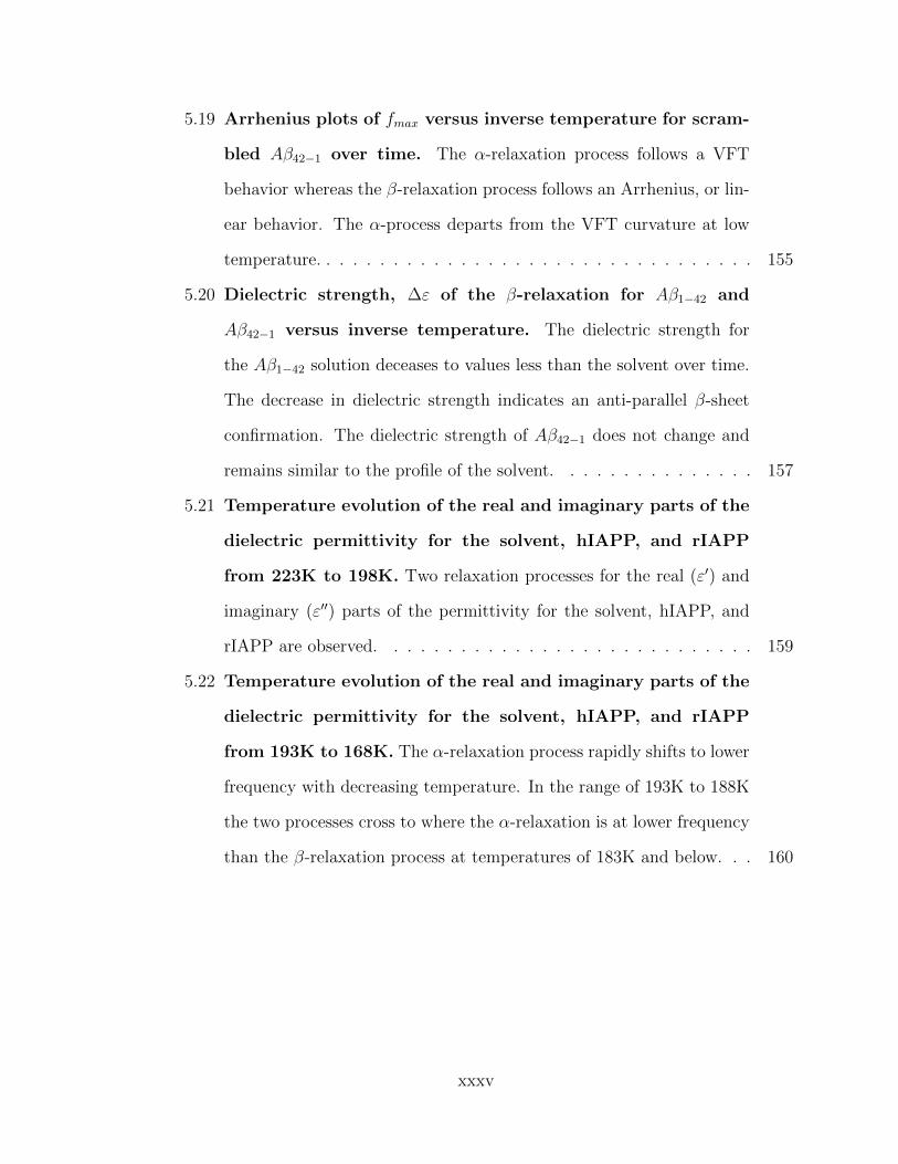
temperature. . . . . . . . . . . . . . . . . . . . . . . . . . . . . . . . . 155
5.20 Dielectric strength, ∆ε of the β-relaxation for Aβ1−42 and
Aβ42−1 versus inverse temperature. The dielectric strength for
the Aβ1−42 solution deceases to values less than the solvent over time.
The decrease in dielectric strength indicates an anti-parallel β-sheet
confirmation. The dielectric strength of Aβ42−1 does not change and
remains similar to the profile of the solvent. . . . . . . . . . . . . . . 157
5.21 Temperature evolution of the real and imaginary parts of the
dielectric permittivity for the solvent, hIAPP, and rIAPP
from 223K to 198K. Two relaxation processes for the real (ε′) and
imaginary (ε′′) parts of the permittivity for the solvent, hIAPP, and
rIAPP are observed. . . . . . . . . . . . . . . . . . . . . . . . . . . . 159
5.22 Temperature evolution of the real and imaginary parts of the
dielectric permittivity for the solvent, hIAPP, and rIAPP
from 193K to 168K. The α-relaxation process rapidly shifts to lower
frequency with decreasing temperature. In the range of 193K to 188K
the two processes cross to where the α-relaxation is at lower frequency
than the β-relaxation process at temperatures of 183K and below. . . 160
xxxv
5.23 Temperature evolution of the real and imaginary parts of the
dielectric permittivity for the solvent, hIAPP, and rIAPP
from 163K to 133K. The β-relaxation process dominates below the
crossing temperature and continues to slow to under 1 Hz. The DC
conductivity has reduced in magnitude to outside the measured range
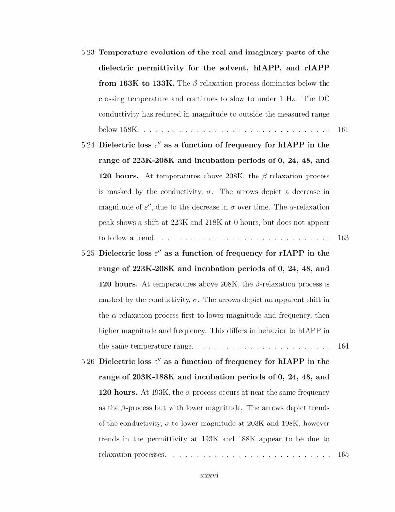
below 158K. . . . . . . . . . . . . . . . . . . . . . . . . . . . . . . . . 161
5.24 Dielectric loss ε′′ as a function of frequency for hIAPP in the
range of 223K-208K and incubation periods of 0, 24, 48, and
120 hours. At temperatures above 208K, the β-relaxation process
is masked by the conductivity, σ. The arrows depict a decrease in
magnitude of ε′′, due to the decrease in σ over time. The α-relaxation
peak shows a shift at 223K and 218K at 0 hours, but does not appear
to follow a trend. . . . . . . . . . . . . . . . . . . . . . . . . . . . . . 163
5.25 Dielectric loss ε′′ as a function of frequency for rIAPP in the
range of 223K-208K and incubation periods of 0, 24, 48, and
120 hours. At temperatures above 208K, the β-relaxation process is
masked by the conductivity, σ. The arrows depict an apparent shift in
the α-relaxation process first to lower magnitude and frequency, then
higher magnitude and frequency. This differs in behavior to hIAPP in
the same temperature range. . . . . . . . . . . . . . . . . . . . . . . . 164
5.26 Dielectric loss ε′′ as a function of frequency for hIAPP in the
range of 203K-188K and incubation periods of 0, 24, 48, and
120 hours. At 193K, the α-process occurs at near the same frequency
as the β-process but with lower magnitude. The arrows depict trends
of the conductivity, σ to lower magnitude at 203K and 198K, however
trends in the permittivity at 193K and 188K appear to be due to
relaxation processes. . . . . . . . . . . . . . . . . . . . . . . . . . . . 165
xxxvi
5.27 Dielectric loss ε′′ as a function of frequency for rIAPP in the
range of 203K-188K and incubation periods of 0, 24, 48, and
120 hours. At 193K, the α-process occurs at near the same frequency
as the β-process but with lower magnitude. At 193K and 188K, there
are some shifts in the the conductivity, σ, but it does not appear to
follow a trend over time. . . . . . . . . . . . . . . . . . . . . . . . . . 166
5.28 Dielectric loss ε′′ as a function of frequency for hIAPP in the
range of 183K-168K and incubation periods of 0, 24, 48, and
120 hours. In the range of 183K-168K, there is significant mixing
between σ, α-, and β-processes. Trends in this range are indeterminate. 167
5.29 Dielectric loss ε′′ as a function of frequency for rIAPP in the
range of 183K-168K and incubation periods of 0, 24, 48, and
120 hours. In the range of 183K-168K, there is significant mixing
between σ, α-, and β-processes. Trends in this range are indeterminate. 168
5.30 Dielectric loss ε′′ as a function of frequency for hIAPP in
the range of 163K-148K and incubation periods of 0, 24, 48,
and 120 hours. At 158K, the conductivity, σ and the α-process are
substantially separated from the β process. At 158K and below, the β-
relaxation peak in ε′′ trends to higher magnitude and lower frequency
over time. . . . . . . . . . . . . . . . . . . . . . . . . . . . . . . . . . 169
xxxvii
5.31 Dielectric loss ε′′ as a function of frequency for rIAPP in the
range of 163K-148K and incubation periods of 0, 24, 48, and
120 hours. At 158K, the conductivity, σ and the α-process are sub-
stantially separated from the β process. At 158K and below, the β-
relaxation peak first shifts to lower frequency and higher magnitude,
then shifts to higher frequency and lower magnitude towards the spec-
tra of the solvent. This differs in behavior from that of hIAPP in the
same temperature range. . . . . . . . . . . . . . . . . . . . . . . . . . 170
5.32 Dielectric loss ε′′ as a function of frequency for hIAPP in the
range of 143K-133K and incubation periods of 0, 24, 48, and
120 hours. The β-relaxation peak in ε′′ trends to higher magnitude
and lower frequency over time. . . . . . . . . . . . . . . . . . . . . . . 171
5.33 Dielectric loss ε′′ as a function of frequency for rIAPP in the
range of 143K-133K and incubation periods of 0, 24, 48, and
120 hours. The β-relaxation peak first shifts to lower frequency and
higher magnitude, then shifts to higher frequency and lower magnitude
towards the spectra of the solvent. This differs in behavior from that
of hIAPP in the same temperature range. . . . . . . . . . . . . . . . . 172
5.34 Curve fitting of imaginary part of the permittivity data using
the WinFIT program of the solvent, hIAPP, and rIAPP at
223K. A large, low frequency DC conductivity is fit with a power
law. The α-relaxation process at around 107 Hz is fit with a Havriliak-
Negami function. The β-relaxation function is not observed. The
RMSD of the fits are 0.015, 0.016, and 0.034, respectively. . . . . . . 174
xxxviii

5.35 Curve fitting of imaginary part of the permittivity data using
the WinFIT program of the solvent, hIAPP, and rIAPP at
208K. A large, low frequency DC conductivity is fit with a power law.
The β-relaxation process at around 103 Hz is fit with a Cole-Davidson
function and the α-relaxation process at around 105 Hz is fit with a
Havriliak-Negami function. The RMSD of the fits are 0.018, 0.007, and
0.020, respectively. . . . . . . . . . . . . . . . . . . . . . . . . . . . . 175
5.36 Curve fitting of imaginary part of the permittivity data using
the WinFIT program of the solvent, hIAPP, and rIAPP at
188K. A large, low frequency DC conductivity is fit with a power law.
The β-relaxation process at around 103 Hz is fit with a Cole-Davidson
function and the α-relaxation process at around 101 Hz is fit with a
Havriliak-Negami function. Here, the α process has crossed over to
slower than β relaxation times. The RMSD of the fits are 0.001, 0.006,
and 0.008, respectively. . . . . . . . . . . . . . . . . . . . . . . . . . . 176
5.37 Curve fitting of the imaginary part of the permittivity data
using the WinFIT program of the solvent, hIAPP, rIAPP
at 133K. A small, very low frequency DC conductivity is fit with a
power law. The β-relaxation process at around 1 Hz is fit with a Cole-
Davidson function and the α-relaxation process is not observed. The
RMSD of the fits are 0.073, 0.090, and 0.035, respectively. . . . . . . 177
5.38 Arrhenius plots of fmax versus inverse temperature for solvent
over time. The α-relaxation process follows a VFT behavior whereas
the β-relaxation process follows an Arrhenius, or linear behavior. . . . 178
xxxix

5.39 Arrhenius plots of fmax versus inverse temperature for hIAPP
from 0-120 hours. The α-relaxation process follows a VFT behavior
whereas the β-relaxation process follows an Arrhenius, or linear behav-
ior. The α-process departs from the VFT curvature at low temperature.179
5.40 Arrhenius plots of fmax versus inverse temperature for rIAPP
from 0-120 hours. The α-relaxation process follows a VFT behavior
whereas the β-relaxation process follows an Arrhenius, or linear behav-
ior. The α-process departs from the VFT curvature at low temperature.180
5.41 Dielectric strength, ∆ε of the β-relaxation for hIAPP and
rIAPP versus inverse temperature. The dielectric strength for the
hIAPP solution remains relatively constant for the first 48 hours, then
deceases to values less than the solvent after 120 hours of incubation.
This may be an indication that the final aggregated state of hIAPP in
serum is an anti-parallel β-sheet. The dielectric strength of rIAPP was
similar to the solvent for all time points. This is a similar ∆ε behavior
of Aβ1−42 and Aβ42− 1 observed for the same solvent. . . . . . . . . 183
5.42 Plots of the β-relaxation peak shift at 143K for Aβ1−42/Aβ42−1
and hIAPP/rIAPP as compared to the solvent. The amyloido-
genic peptides demonstrate a characteristic ”red- shift” towards tower
frequencies, indicating an increase in structured water. . . . . . . . . 185
xl

Chapter 1
Introduction
1.1 Motivation for the Studies of Amyloidogenic
Peptides
Improved patient care coupled with higher standards of living has nearly doubled
the average life span of a person over the past century [1]. Furthermore, the leading
edge of the ”baby boom” generation is now approaching the midlife mark causing an
influx of aged persons. The result of an increasingly older population is a record high
incidence of aging-related diseases that is projected to triple over the next 40 years
[2].
Many of these diseases are attributed to misfolded, aggregated proteins known as
amyloids. Amyloids collect in the tissues and organs such as the brain, pancreas, and
spleen causing debilitating diseases such as Alzheimer’s and Type II Diabetes Mellitus.
Each disease is associated with a particular protein responsible for the pathologic
effects of amyloidogenic diseases, or amyloidoses. Although there have been several
attempts to develop diagnostic methods based on the detection of amyloidogenic
oligomers, there is an absence of a widely-accepted and deterministic approach.
1

Alzheimer’s disease
Alzheimer’s Disease (AD) is the most common cause of senile dementia. AD is an
age-associated neurodegenerative disorder that causes loss of memory and language
skills, damaged cognitive function, and altered behavior. AD typically affects people
over the age of 65, but can start as early as people in their 30s [3].
It is estimated that 5.4 million Americans are living with AD, including approxi-
mately 200,000 age 65 years or younger with the aging of the baby boom generation
projected to result in an additional 10 million people with AD in the near future. By
2050, there is expected to be nearly a million new cases per year, and AD prevalence
is projected to be 11 to 16 million [4].
AD is the sixth leading cause of death in the United States and the fifth leading
cause of death in Americans age ≥65 years. Although the proportions of deaths due
to other major causes of death have decreased in the last several years, the proportion
of deaths due to AD has risen significantly by a staggering 66% [4].
In 2011, more than 15 million family members and other unpaid caregivers pro-
vided an estimated 17.4 billion hours of care to people with AD and other dementias.
In 2012, payments for health care, long-term care, and hospice services for people
age ≥65 years with AD and other dementias are expected to be $200 billion. An
estimated 800,000 people with AD (one in seven) live alone, and up to half of them
do not have an identifiable caregiver [4].
Diabetes mellitus
Diabetes mellitus is the most common endocrine disease, characterized by high glucose
levels, or hyperglycemia. The source of hyperglycemia may be due to either reduced
insulin secretion or inaction by the body to properly use insulin. Common symptoms
of diabetes are polyuria, polydypsia, polyphagia, weight loss, fatigue, blurred vision,
and numbness [5].
2

There are four main types of diabetic disorders: Type I, Type II, gestational, and
diabetes induced from other illnesses, such as pancreatic cancer or liver disfunction.
Type I diabetes is also known as insulin-dependent or juvenile onset diabetes and
occurs due to a loss of insulin-producing pancreatic β-cells. Type II diabetes is also
known as non-insulin depended or adult onset diabetes. Type II diabetes occurs due
to an insulin resistance and decreased production of insulin by pancreatic β-cells.
In Type II diabetic patients, the muscles, liver, and fat cells cannot use the insulin
produced in the body which leads to high levels of insulin [5].
Diabetes mellitus affects 25.8 million people of all ages-approximately 8.3 % of the
U.S. population. Among U.S. residents ages 65 years and older, 10.9 million, or 26.9
%, had diabetes in 2010. About 1.9 million people ages 20 years or older were newly
diagnosed with diabetes in 2010 in the United States. A study in 2005-2008 found
that 35 % of U.S. adults ages 20 years or older and 50 % of adults ages 65 years or
older had signs of prediabetes [6].
Diabetes is the leading cause of kidney failure, nontraumatic lower-limb amputa-
tions, and new cases of blindness among adults in the United States. It is also one of
the major causes of heart disease and stroke and the seventh leading cause of death
in the United States [6].
Direct medical costs are estimated at $116 billion in 2010. Average medical ex-
penditures among people with diagnosed diabetes were 2.3 times higher than what
expenditures would be in the absence of diabetes. Indirect costs such as disability,
work loss, premature mortality are estimated at $58 billion [6].
1.1.1 Pathogenesis of amyloidogenic diseases
Amyloidosis is a pathological condition that refers to a number of diseases charac-
terized by the formation of insoluble amyloid deposits in tissues and organs, such
as liver, spleen, kidneys, and brain [7]. The deposits are caused by the misfolding
3
and aggregation of amyloidogenic peptides into organized, fibrillar structures. Exam-
ples of the most common amyloid-related diseases are Alzheimer’s disease, Type II
diabetes, Huntington’s disease, Parkinson’s disease, Creutzfeldt-Jakob disease, and
even transmissible diseases, such as spongiform encephalopathies [8]. Each disease
has its own characteristic amyloidogenic peptide responsible for tissue and organ de-
struction. Although the etiology is varied (Genetic, sporadic, and infectious) [9], all
present the characteristic amyloid plaque deposits in tissues that can be imaged ex
vivo via histopathologic staining.
Historically, the amyloid hypothesis implicated amyloid plaques as the primary
cause of amyloidogenic diseases [10, 11]. Recent evidence shows that organ and tissue
disruption begins with aggregation of soluble, pre-fibrillar oligomers [12, 13, 14, 15].
Soluble amyloidogenic peptides have been found in cerebral spinal fluid (CSF) [16],
urine [17], and blood [18], but currently there is no diagnostic method. Early detection
of pre-fibrillar oligomers in any of these media is the motivation of our research.
Pathology of Alzheimer’s disease
Alois Alzheimer first observed fibrils in the port-mortem brains of patients who suf-
fered from a form of dementia now known as Alzheimer’s disease (AD) [19]. Two
physiological abnormalities are present in the brains of patients whom suffered from
AD: intracellular neurofibrillary tangles (NFT) and extracellular amyloid desposits
[20]. NFTs are paired helical filaments of hyperphosphorylated tau protein aggregates
that are commonly found in the brains of patients with neurological disorders [20].
The amyloid deposits between neurons consist mainly of the polypeptides β-amyloid
Aβ1−40 and Aβ1−42 and contrary to NFTs, are only found in patients with AD. Amy-
loid plaques and NFTs collect in the cerebral cortex and hippocampus regions of the
brain[21]. Recent discovery of a pathogenic mutation in the amyloid precursor protein
(APP) suggest that β-amyloid deposition is the primary cause of AD and may cas-
4
cade the formation of hyperphosphorylated tau tangles and eventual neuronal death
[22].
The β-amyloids originate from proteolytic cleavage (hydrolysis of the peptide
bond) of the transmembrane amyloid precursor protein (APP). In a healthy brain,
APP is cleaved by α- then γ-secretase between the lysine (16) and leucine (17) residues
located in the hydrophobic KLVFF (16-20) region [11]. Cleavage of the hydrophobic
region inhibits β-amyloid aggregation and the resulting chain is Aβ17−40 or Aβ17−42,
also known as 3p [23, 11]. In pathogenic proteolytic processing of APP, the chain is
first cleaved by β-secretase, not α-, which results in a longer chain of Aβ1−40 or Aβ1−42,
as depicted in Figure 1.1. Enzymatic processes regulate and destroy pathogenic Aβ,
preventing fibril formation in non-Alzheimer’s patients [24].
β-secretase γ-secretase
APP Aβ (1-40) or (1-42)
711 or 713 671 1 770
COOH NH2
α-secretase γ-secretase
APP p3
687 711 or 713 1 770
COOH NH2
(a)
(b)
Figure 1.1: Non-pathogenic (a) and pathogenic (b) proteolytic processing of APP byα- or β-secretase, followed by γ-secretase cleavage. Adapted from [11].
Early theories about the pathogenesis of β-amyloid suggested that amyloid fibrils
and plaques caused cell damage and death [25]. It is now believed that the oligomer
and protofibril conformations are in fact more toxic because of their pore-forming
capabilities [26, 16]. The molecular mechanism for toxicity is believed due to amyloid-
5
β disruption of the calcium channels at the membrane lipid bilayer through pore
formation [26, 27].
Forms of soluble β-amyloid has been found in a number of fluids in both clinical
AD and non-clinical AD individuals, including cerebral spinal fluid (CSF), blood
plasma, and urine [18, 28]. Therefore, the development of a novel detection method
of the soluble, intermediate oligomeric forms of β-amyloid in one or all of these fluids
is a central focus of our studies.
Pathology of Type II diabetes
Amyloid deposits of human Islet Amyloid Polypeptide (IAPP), also known as amylin,
have been found post-mortem in the pancreatic beta cells of more than 90% of pa-
tients with Type II diabetes [29]. Amylin is co-secreted with insulin by the pancreatic
β-cells in the islets of Langerhans as a regulator of glucose uptake and gastric empty-
ing. The 37 residue polypeptide amylin is soluble and non-toxic in its natural form.
Environmental conditions and genetic predisposition cause amylin to aggregate and
form toxic amyloid fibrils [30]. The amyloid deposits cause death of the pancreatic
β-cells leading to reduced production of insulin and eventually Type II diabetes [31].
Amylin has been found to be amyloidogenic in humans, monkeys, and cats but
not amyloidogenic in hamsters, mice, and rats [32, 33]. The variations in amino acid
sequencies between species points to a theory that specific hydrophobic regions are
responsible for amyloid formation. For example, in human IAPP, sequence 20-29 has
been shown in vivo as a source for amyloid fibril formation [33, 31].
Recent theory suggest that cell membrane toxicity by IAPP is caused by pore-like
disruption by oligomer and protofibril species [12]. The oligomers form ion channels
in the lipid bilayers on the pancreatic β-cell membrane. These small pores allow cell
contents to pass through, causing destabilization and cell death [34]. A cascading
effect then follows where amylin aggregation destroys β-cells leading to decreased
6
insulin. The remaining β-cells try to compensate by releasing more insulin and thus,
more amylin which leads to further destruction of β-cells [35]. It is known that
resulting basal amylin serum concentration is abnormal in patients with Type II
diabetes [36], though the structure of the amylin (i.e. monomers, dimers, oligomers,
etc.) is not classified. Novel detection of the oligomer and protofibril forms of amylin
in blood serum is a central focus of our studies.
1.2 Protein Structure and Amyloidogenic Disease
1.2.1 Protein composition and structure
Proteins are a class of biological polymers responsible for a variety of essential biolog-
ical functions in living systems; they act as reaction catalysts, transport and storage
mechanisms, support immune function, transmit nerve impulses, and control growth
and differentiation[37]. Each protein has a unique structure tailored to serve a specific
biological role [38].
Proteins are comprised of primary building blocks called amino acids. Amino acids
consist of a central carbon atom (α-carbon), amino group, carboxylic acid group,
hydrogen atom, and a side chain (R group). The properties of proteins are mainly
dependent on the characteristics of their composing animo acids, such as capacity to
polymerize, acid-base properties, structure and chirality, and chemical functionality.
Nearly all proteins found in all living organisms are constructed from the same 20
amino acids [37].
Proteins are linear chains of amino acids formed by linking the carboxyl group of
one amino acid to the amine group of the next by a covalent link called a peptide bond
(Figure 1.2). The bond releases a water molecule with the carboxyl group supplying
the oxygen and the amine group supplying the two hydrogens. A series of amino acid
comprising of less than 50 residues is referred to as a polypeptide and is named in the
7
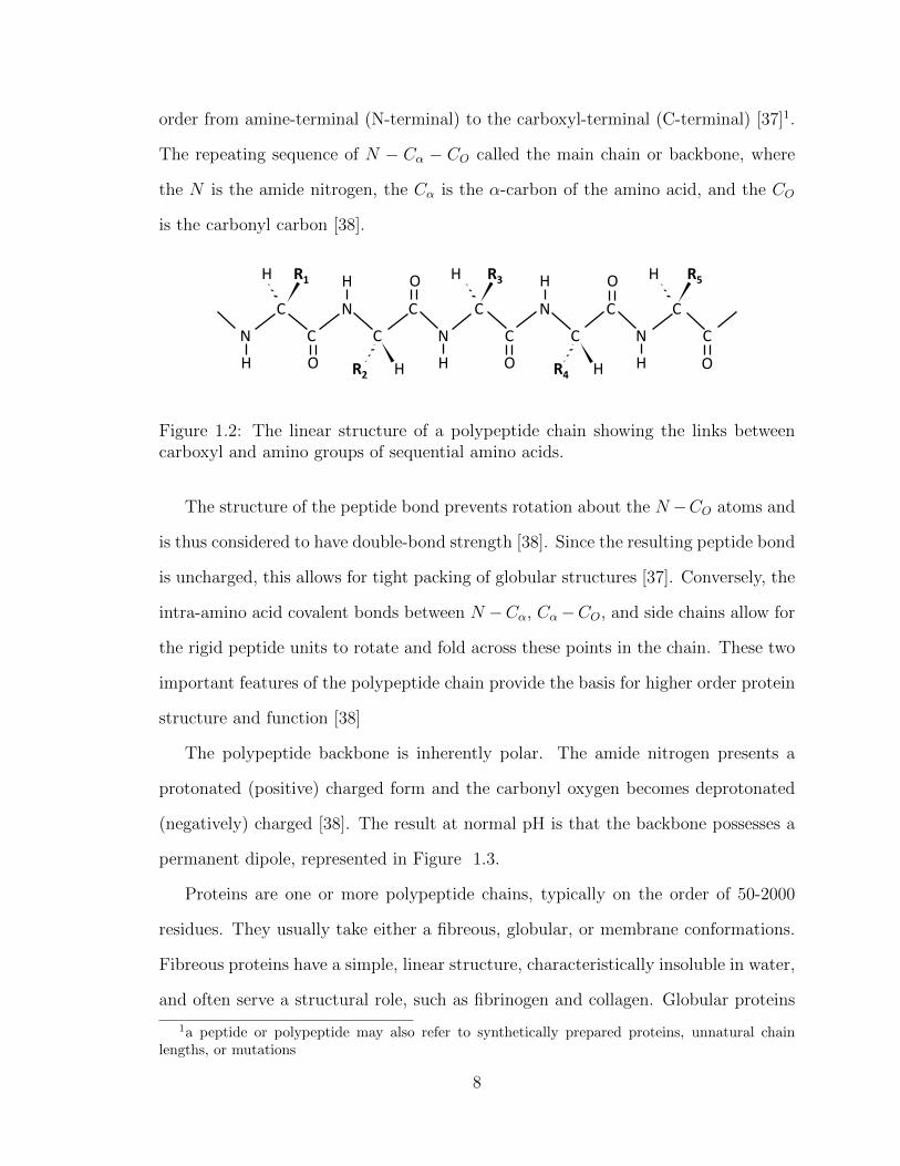
order from amine-terminal (N-terminal) to the carboxyl-terminal (C-terminal) [37]1.
The repeating sequence of N − Cα − CO called the main chain or backbone, where
the N is the amide nitrogen, the Cα is the α-carbon of the amino acid, and the CO
is the carbonyl carbon [38].
R4
CCCCC NNN
CCCC NN
H
C
HH
HHH
OO
OOO
HH
HH
R5R3
R2
R1
Figure 1.2: The linear structure of a polypeptide chain showing the links betweencarboxyl and amino groups of sequential amino acids.
The structure of the peptide bond prevents rotation about the N −CO atoms and
is thus considered to have double-bond strength [38]. Since the resulting peptide bond
is uncharged, this allows for tight packing of globular structures [37]. Conversely, the
intra-amino acid covalent bonds between N −Cα, Cα−CO, and side chains allow for
the rigid peptide units to rotate and fold across these points in the chain. These two
important features of the polypeptide chain provide the basis for higher order protein
structure and function [38]
The polypeptide backbone is inherently polar. The amide nitrogen presents a
protonated (positive) charged form and the carbonyl oxygen becomes deprotonated
(negatively) charged [38]. The result at normal pH is that the backbone possesses a
permanent dipole, represented in Figure 1.3.
Proteins are one or more polypeptide chains, typically on the order of 50-2000
residues. They usually take either a fibreous, globular, or membrane conformations.
Fibreous proteins have a simple, linear structure, characteristically insoluble in water,
and often serve a structural role, such as fibrinogen and collagen. Globular proteins
1a peptide or polypeptide may also refer to synthetically prepared proteins, unnatural chainlengths, or mutations
8

COO- NH3+
C
H R
dipole moment
Figure 1.3: Amino acids and consequently, the polypeptide backbone consists of onepositively charged and one negatively charged end. This produces a permanent dipolemoment.
take an approximate spherical shape and are soluble in water. Most enzymes and
myoglobin are examples of globular proteins. Membrane proteins have hydropho-
bic side chains oriented outward so that they can interact with the non-polar phase
within membranes. Membrane proteins are insoluble in water but often soluble in
detergents and other non-polar compounds. The light-absorbing proton pump, bac-
teriorhodopsin is an example of a typical membrane protein [38].
Proteins are classified into a structural hierarchy by their composition and con-
formation. The simplest form is the primary structure, or linear polypeptide chain.
The secondary structure of proteins represents a three-dimensional arrangement of
polypeptides formed by hydrogen bonding between amino acids that are in spatial
proximity, but not necessarily neighboring. Secondary structure proteins may take the
form of either a twisted α-helix or pleated β-strand that extends along one-dimension.
Diagrammatic representations of both conformations are shown in Figure 1.4. The
tertiary structure is characterized by a compact three-dimensional arrangement by
bending or folding of the polypeptide chains. Globular proteins are organized by a
tertiary structure. The tertiary structure may be stabilized by the formation of co-
valent bonds, such as ionic, disulfide and salt bridges, or non-covalent bonds, such as
van der Waals forces and hydrogen bonds. The quaternary structure is a combina-
9
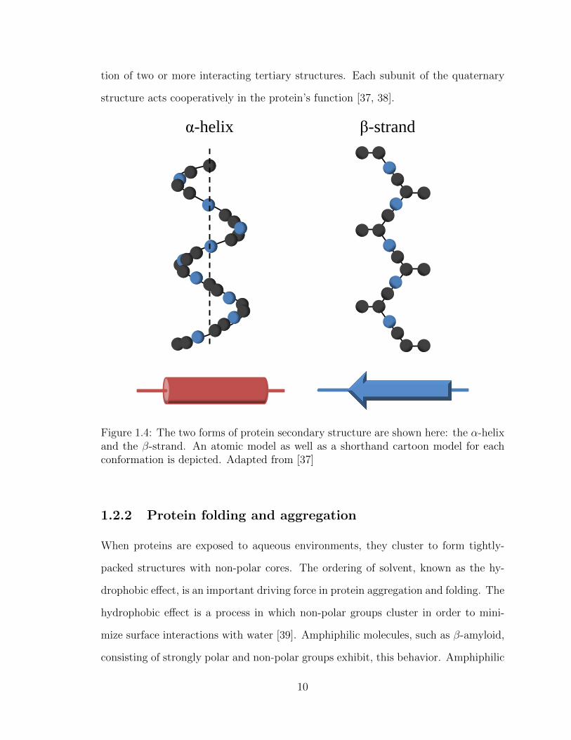
tion of two or more interacting tertiary structures. Each subunit of the quaternary
structure acts cooperatively in the protein’s function [37, 38].
α-helix β-strand
Figure 1.4: The two forms of protein secondary structure are shown here: the α-helixand the β-strand. An atomic model as well as a shorthand cartoon model for eachconformation is depicted. Adapted from [37]
1.2.2 Protein folding and aggregation
When proteins are exposed to aqueous environments, they cluster to form tightly-
packed structures with non-polar cores. The ordering of solvent, known as the hy-
drophobic effect, is an important driving force in protein aggregation and folding. The
hydrophobic effect is a process in which non-polar groups cluster in order to mini-
mize surface interactions with water [39]. Amphiphilic molecules, such as β-amyloid,
consisting of strongly polar and non-polar groups exhibit, this behavior. Amphiphilic
10

molecules form micelles in which the non-polar ends combine to form a hydrophobic
domain of hydrocarbon tails while polar ends have ionic interactions with the sol-
vent [37]. Figure 1.5 shows the burying of internal hydrophobic regions in micelle
formation.
hydrophilic head
hydrophobic tail
micelle
Figure 1.5: Hydrophobic tails bury in the interior during micelle formation as hy-drophilic regions interact with polar solvents.
The immediate layers of water molecules surrounding the protein is known as the
hydration shell. When a protein is placed in water, the hydration shell is disturbed.
The water competes with the hydrogen bonding in the hydrophobic domain of the
protein causing a reordering of the bound water. The bound water is then released
and the hydrophobic regions begin to cluster. This is driven by a thermodynamically
favorable event where the movement of bound, ordered water, moves to free, bulk-like
water in the direction of increased entropy [37]. When a protein folds, the hydropho-
bic and hydrophilic regions combine via non-covalent interactions to form secondary
structures, such as α-helices and β-sheets. The α-helix is formed by hydrogen bonds
between NH and CO groups of the main chain. Figure 1.6 shows the β-sheet con-
formation is formed by either parallel or anti-parallel stacking between polypeptide
strands [37, 38].
11
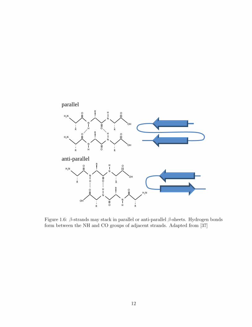
parallel
anti-parallel
H2N
N
N
O
O
O
OH
H
H R R
R
H2N
N
N
O
O
O
OH
H
H R R
R
H2N
N
N
O
O
O
OH
H
H R R
R
H2N
N
N
O
O
O
OH
H
H R R
R
Figure 1.6: β-strands may stack in parallel or anti-parallel β-sheets. Hydrogen bondsform between the NH and CO groups of adjacent strands. Adapted from [37]
12
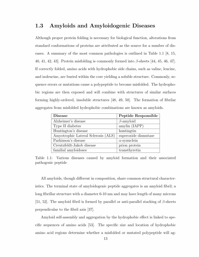
1.3 Amyloids and Amyloidogenic Diseases
Although proper protein folding is necessary for biological function, alterations from
standard conformations of proteins are attributed as the source for a number of dis-
eases. A summary of the most common pathologies is outlined in Table 1.1 [8, 15,
40, 41, 42, 43]. Protein misfolding is commonly formed into β-sheets [44, 45, 46, 47].
If correctly folded, amino acids with hydrophobic side chains, such as valine, leucine,
and isoleucine, are buried within the core yielding a soluble structure. Commonly, se-
quence errors or mutations cause a polypeptide to become misfolded. The hydropho-
bic regions are then exposed and will combine with structures of similar surfaces
forming highly-ordered, insoluble structures [48, 49, 50]. The formation of fibrilar
aggregates from misfolded hydrophobic combinations are known as amyloids.
Disease Peptide Responsible
Alzheimer’s disease β-amyloidType II diabetes amylin (IAPP)Huntington’s disease huntingtinAmyotrophic Lateral Sclerosis (ALS) superoxide dismutaseParkinson’s disease α-synucleinCreutzfeldt-Jakob disease prion proteinfamilial amyloidoses transthyretin
Table 1.1: Various diseases caused by amyloid formation and their associatedpathogenic peptide
All amyloids, though different in composition, share common structural character-
istics. The terminal state of amyloidogenic peptide aggregates is an amyloid fibril; a
long fibrillar structure with a diameter 6-10 nm and may have length of many microns
[51, 52]. The amyloid fibril is formed by parallel or anti-parallel stacking of β-sheets
perpendicular to the fibril axis [37].
Amyloid self-assembly and aggregation by the hydrophobic effect is linked to spe-
cific sequences of amino acids [53]. The specific size and location of hydrophobic
amino acid regions determine whether a misfolded or mutated polypeptide will ag-
13

gregate to form the β-sheet structure and ultimately, amyloid fibrils. Hydrophobic
regions that are normally hidden in a properly folded protein are exposed to favor fib-
ril formation by the surrounding solvent. Electrostatic and hydrophobic interactions
cause these hydrophobic regions to combine into higher ordered structures.
Fibril formation begins with monomers, dimers, and small oligomers combining
to form a pre-fibrilar oligomer nucleus. Once the nucleus is formed, monomers attach
longitudinally to the core to create elongated protofibril strands (Figure 1.7) [54,
55]. Hydrogen bonds between elongated protofibrils then stack together laterally
in parallel combinations to form fibril strands, as shown in Figure 1.8 [56]. The
hydrogen bond network of the cross-β spine between β-strands creates insoluble and
extremely stable fibrils [55].
Aβ monomers amyloid oligomer
nucleus
amyloid protofibril amyloid fibril
Figure 1.7: Nucleation starts with oligomer formation of β-amyloid fragments.Monomers then attach longitudinally to the oligomeric nucleus.
14
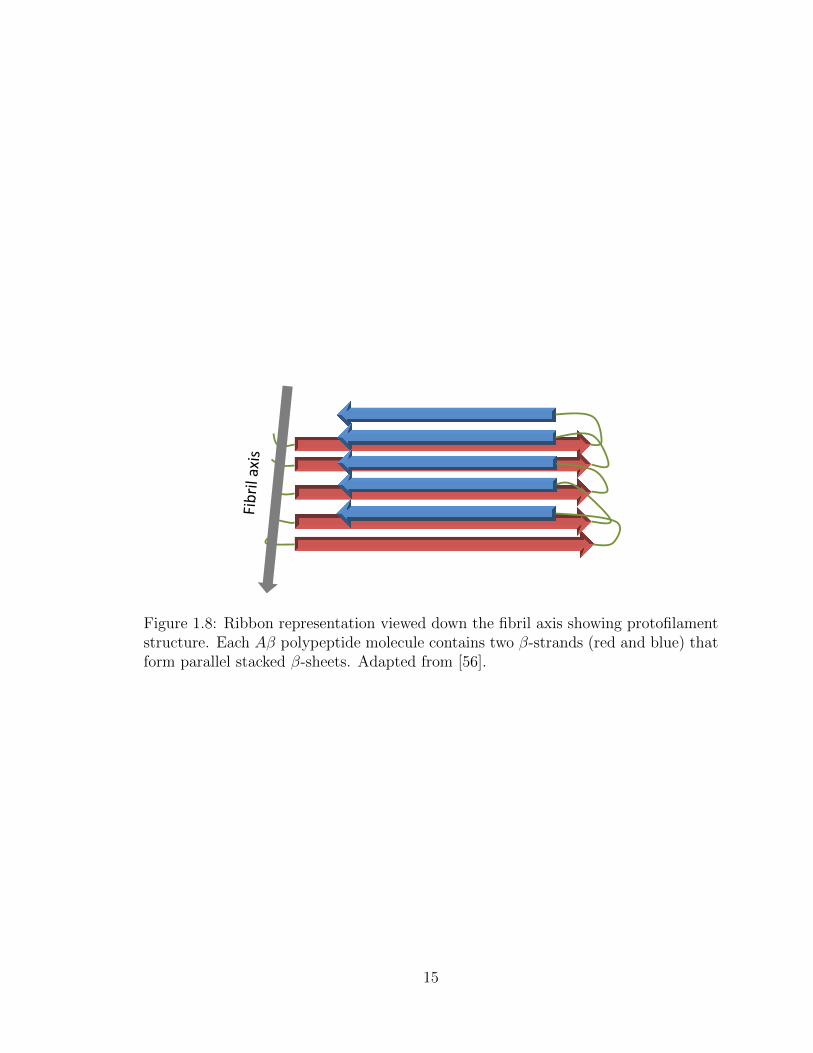
Figure 1.8: Ribbon representation viewed down the fibril axis showing protofilamentstructure. Each Aβ polypeptide molecule contains two β-strands (red and blue) thatform parallel stacked β-sheets. Adapted from [56].
15
1.4 The Role of Biological Water
Water plays a crucial role in protein hydration dynamics. Proteins are not static
structures, but rather undergo a variety of fluctuations such as vibrations and rota-
tions [57]. Recent theories suggest that water controls large-scale motions and shape
changes as well as control internal motions necessary for function [58, 59, 57, 60, 61,
62]. Water mediated motions in proteins can be studied by modeling the α and β
fluctuations that are traditionally observed in glass-forming materials [63, 59].
The dynamics of water interactions vary in regards to the location with respect to
a protein. Biological water can be classified into three main groups: bulk-like or free
water, surface or bound water, and internal or caged water [64]. Figure 1.9 shows
the distribution of the three types of biological water at the protein-water interface
using Aβ1−42 structure as an example (obtained from Protein Data Bank ID: 1IYT
[65]). Each classification of biological water plays a role in the dynamics and function
of proteins.
Bulk-like water is located in the region beyond the first few molecules of the
protein surface. It resembles pure water in structure, properties, and function. Bulk
water plays a role in large-scale motions and shape changing as described by the α
fluctuations of a hydrated protein solution [59]. We hypothesize that during amyloid
aggregation, changes to the α fluctuations can be observed in the dielectric spectra.
Bound water is located at the surface of proteins where their hydrogen bond net-
works can interact with amino acid side chains and other surface water molecules
[66]. The diversity of protein composition and structure present varying and unique
forms of bound water. Chemical composition, hydrophobicity, size, and shape of a
protein will determine the behavior of bound water. Bound water at the hydration
layer of proteins is described by internal motions and protein function, known as β
fluctuations [59]. Our hypothesis is that changes to the surface properties of pro-
16
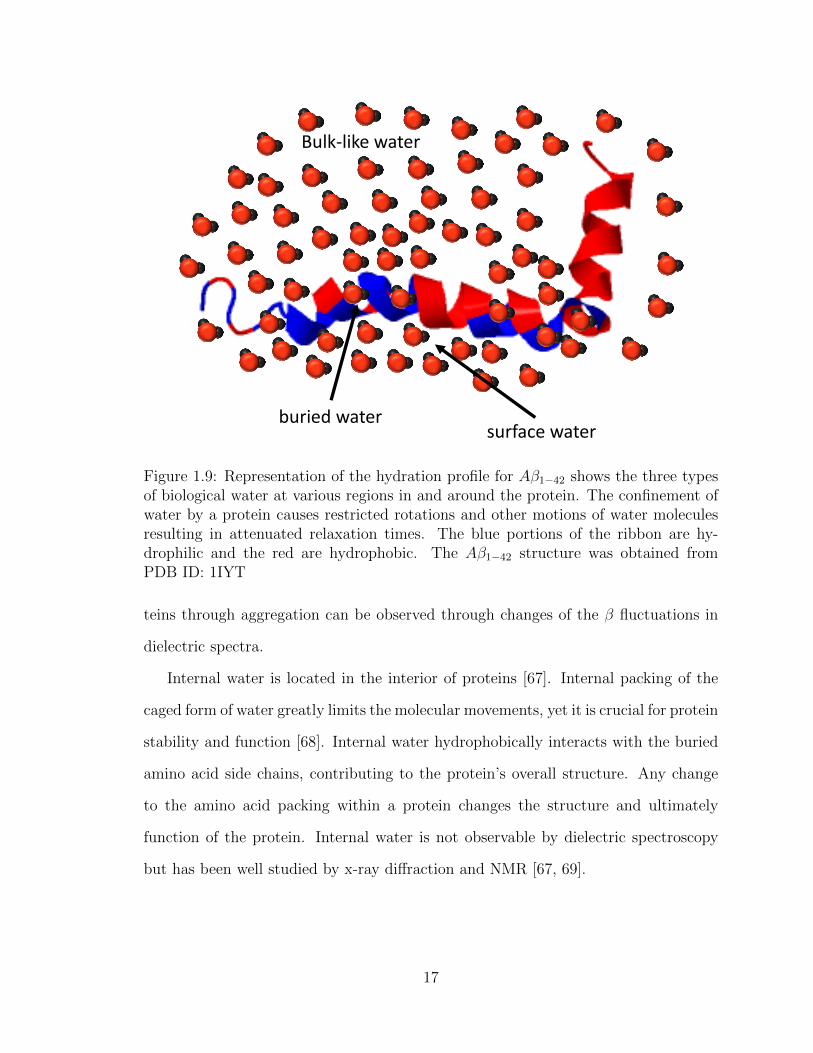
Bulk-like water
surface water buried water
Figure 1.9: Representation of the hydration profile for Aβ1−42 shows the three typesof biological water at various regions in and around the protein. The confinement ofwater by a protein causes restricted rotations and other motions of water moleculesresulting in attenuated relaxation times. The blue portions of the ribbon are hy-drophilic and the red are hydrophobic. The Aβ1−42 structure was obtained fromPDB ID: 1IYT
teins through aggregation can be observed through changes of the β fluctuations in
dielectric spectra.
Internal water is located in the interior of proteins [67]. Internal packing of the
caged form of water greatly limits the molecular movements, yet it is crucial for protein
stability and function [68]. Internal water hydrophobically interacts with the buried
amino acid side chains, contributing to the protein’s overall structure. Any change
to the amino acid packing within a protein changes the structure and ultimately
function of the protein. Internal water is not observable by dielectric spectroscopy
but has been well studied by x-ray diffraction and NMR [67, 69].
17
1.5 Dielectric Spectroscopy as a Tool for Studying
Amyloidogenic Peptides
Dielectric relaxation spectroscopy (DRS) is an effective technique for the study and
characterization of biological materials and systems. The non-invasive nature of the
technique allows for in situ monitoring of processes in a variety of environments. For
decades, DRS has been using to study the dynamics of water at protein interfaces
[70, 71, 72, 73]. Water structure near the surfaces of proteins is subject to hydrogen
bonding of water molecules to proteins and electrostatic interactions due to the large
dipole moment [74]. Studies of relaxation processes give us insight into structural and
dynamical properties of biomaterials.
DRS allows the study of thermal fluctuations of supercooled liquids and glasses
by relaxation measurements. Fluctuations and relaxations are interconnected by the
fluctuation-dissipation theorem, which states that the same phenomena, observed un-
der small perturbations, must also occur at equilibrium. Meaning that, observations
of relaxation dynamics are representative of equilibrium fluctuations. Since protein
structure and function are slaved to solvent behavior [58], this has great significance
in the study of protein dynamics [75]. Application of an external electric field to
a material provides the thermodynamical disturbance that can then be studying by
relaxation spectroscopy.
The studies presented in this thesis probe the dynamics of proteins over a wide
range of temperatures. The glass-forming cryoprotectant, glycerol is used as a buffer
to study processes at supercooled temperatures. In many glass forming materials,
a number of relaxation processes will present as peaks in dielectric loss, ε′′ over a
broadband of frequencies. They are typically termed in order of increasing frequency,
α-, β-, δ-, and γ-relaxations [63]. It is important to note that the observed relax-
18

ation processes do not originate in the protein itself, but in the bulk solvent and the
hydration shell [59].
α-relaxation
The α-relaxation occurs at low frequency, 101 − 105 Hz. The α process describes
structural fluctuations, as described by the mechanical Maxwell relation [59],
kα(T ) = G0/η(T ) (1.1)
where kα(T ) is the rate coefficient for the α fluctuations to the viscosity η(T ) and
the infinite-frequency shear modulus G0. At low temperature where the material
acts as a solid, the viscosity is extremely large and therefore the α-fluctuations are
essentially absent. The rate coefficient of α fluctuations typically follow the Vogel-
Fulcher-Tammann relation [63].
β-relaxation
The β-relaxation occurs in the radio frequency, 105 − 107 Hz. β processes in super-
cooled liquids and glasses are essentially independent of viscosity and will exist even
at glassy states where we expect α fluctuations to disappear [76, 77, 59]. The β fluctu-
ations take two forms in molecular liquids [78, 79, 80]. The Johari-Goldstein fluctua-
tions are intertwined with the α fluctuations, and at high temperature (>300K), they
merge[81]. Another form of β fluctuations occur as a non-cooperative process that
does not merge with the α process. In contrast, this β process is at lower frequency
than the α process above a crossing temperature [59]. This later form of the βh
relaxation, where h denotes hydration is observed in our studies of protein-solvent in-
teractions. The rate coefficient of β fluctuations typically follow an Arrhenius relation
[63].
19
δ-relaxation
The δ-relaxation occurs in the radio-microwave frequency, 108 − 1010 Hz. The δ
process may possibly be representative of the dynamics of water near a biomolecule
as an exchange between free and bound water states [82, 83, 74]. This process is out
of the range of our measurement apparatus and will not be explored in this thesis.
γ-relaxation
The γ-relaxation occurs in the microwave frequency, 1010−1012 Hz. This frequency is
typical of the relaxation of bulk or free water [74, 84] at distances of many molecules
from the protein surface. This process is out of the range of our measurement appa-
ratus and will not be explored in this thesis.
1.6 A Review of Methods for Studying Amyloido-
genic Peptides
Studies of amyloids in vitro have been effective models for in vivo phenomena [85,
18]. Researchers have been able to observe mechanisms of fibril formation, structure,
and kinetics though a variety of approaches, each with their own advantages and
limitations. Table 1.2 outlines a summary of methods used in the studies of amyloid
structure and aggregation that have provided a baseline for our work. Our goal is to
show that dielectric spectroscopy is an effective tool for early detection of pre-amyloid
structures.
Broadband dielectric relaxation spectroscopy (BDS or DRS) has not been exten-
sively used in the studies of amyloidogenic peptides. One published study on amyloid
fibril formation by DRS was done in non-in vivo-like conditions and lacks a non-
amyloidogenic peptide control [86]. The full capabilities of DRS as an analysis tool of
20

amyloidogenic structures has yet to be explored. The α and β fluctuations due to the
protein and the solvent can be observed through modulation of the dielectric signal.
21
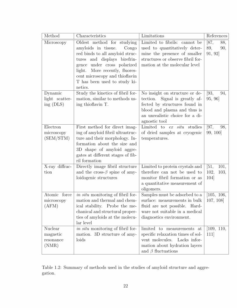
Method Characteristics Limitations References
Microscopy Oldest method for studyingamyloids in tissue. Congored binds to all amyloid struc-tures and displays birefrin-gence under cross polarizedlight. More recently, fluores-cent microscopy and thioflavinT has been used to study ki-netics.
Limited to fibrils: cannot beused to quantitatively deter-mine the presence of smallerstructures or observe fibril for-mation at the molecular level
[87, 88,89, 90,91, 92]
Dynamiclight scatter-ing (DLS)
Study the kinetics of fibril for-mation, similar to methods us-ing thioflavin T.
No insight on structure or de-tection. Signal is greatly af-fected by structures found inblood and plasma and thus isan unrealistic choice for a di-agnostic tool
[93, 94,95, 96]
Electronmicroscopy(SEM/STM)
First method for direct imag-ing of amyloid fibril ultrastruc-ture and their morphology. In-formation about the size and3D shape of amyloid aggre-gates at different stages of fib-ril formation
Limited to ex situ studiesof dried samples at cryogenictemperatures.
[97, 98,99, 100]
X-ray diffrac-tion
Directly image fibril structureand the cross-β spine of amy-loidogenic structures
Limited to protein crystals andtherefore can not be used tomonitor fibril formation or asa quantitative measurement ofoligomers.
[51, 101,102, 103,104]
Atomic forcemicroscopy(AFM)
in situ monitoring of fibril for-mation and thermal and chem-ical stability. Probe the me-chanical and structural proper-ties of amyloids at the molecu-lar level
Samples must be adsorbed to asurface: measurements in bulkfluid are not possible. Hard-ware not suitable in a medicaldiagnostics environment.
[105, 106,107, 108]
Nuclearmagneticresonance(NMR)
in situ monitoring of fibril for-mation. 3D structure of amy-loids
limited to measurements atspecific relaxation times of sol-vent molecules. Lacks infor-mation about hydration layersand β fluctuations
[109, 110,111]
Table 1.2: Summary of methods used in the studies of amyloid structure and aggre-gation.
22
1.7 Thesis Scope and Outline
Recent theories suggest that protein function and dynamics are connected to solvent
interaction and hydration [59]. Protein structure and the hydration profile can be
observed by measuring α and β fluctuations of the solvent-protein solution. Our
hypothesis is that changes in the dielectric permittivity of protein-solvent relaxations
can be observed during amyloid aggregation and fibril formation using the method
of dielectric relaxation spectroscopy (DRS). We expect that the oligomeric form of
amyloid aggregates will display a unique dielectric profile from that of monomers
and fibrils. Characteristics such as space-charge polarization, dipole moment, and
dielectric loss are used to profile the aggregation stages of the peptides.
We discuss the experimental portion in Chapter 3 with the studies of amyloido-
genic peptides in a deionized water buffer at room temperature. The amyloidogenic
human IAPP and β-amyloid and their non-amyloidogenic analogs, rat IAPP and
scrambled β-amyloid are measured by DRS over time and with three concentrations.
The dielectric modulus representation is used to present the conductivity and space-
charge polarization effects measured over seven days of incubation.
We continue in Chapter 4 by studying the same peptides in a 50-50% by weight
deionized water and glycerol buffer. The use of glycerol allows us to study the dielec-
tric signal at sub-freezing temperatures and model the temperature evolution of the
various peptides at different incubation times. Each time point represents a different
fraction of monomers, oligomers, and fibrils. Analysis of the dielectric spectra pro-
vides information about activation energies (enthalpy) and glass-forming fragility for
each time point in an effort to characterize the phase of aggregation. The dielectric
strength for each time and temperature point give information about the dipole mo-
ment of the protein-solvent solutions to determine the structure, whether parallel or
anti-parallel β-sheets.
23
We conclude the experimental portion in Chapter 5 by measuring the peptides
in an in vivo-like condition using serum. The peptides are first diluted in a bovine
serum albumin (BSA) buffer and then diluted in 50-50% by weight glycerol mixture.
Again, the peptide solutions are measured at low temperature and as a function of
time. Activation energies and fragilities are determined and an attempt to classify the
conformations of the peptides is made. The dielectric strength is used to determine
the structural nature of the peptides in the BSA buffer.
We summarize in Chapter 6 the general conclusions of these studies of amyloido-
genic peptides by dielectric relaxation spectroscopy. A direction for future work is
presented for continuation beyond the scope of this thesis.
24
Chapter 2
Materials and Methods
2.1 Introduction to Dielectric Relaxation Spec-
troscopy
The study of the propagation of electric fields in matter is of great interest to physi-
cists, chemists, biologist, and engineers. Not all matter responds to electric fields
in a consistent manner, yet most can be classified into two groups–conductors and
insulators (or dielectrics). Conductors can be considered as possessing an unlimited
amount of charge carriers that are free to move about a material. The electrons in a
conductor are not bound to a particular nucleus but will transfer between molecules
of the substance. By contrast, the electrons of an insulator or dielectric will remain
with the nucleus as a bound ensemble within an atom or molecule [112]. However,
when placed in an electric field the atom or molecule may deform or reorient based on
a mechanism known as polarization. In the dynamic regime, there exists a lag phase
between when the electric field is switched on and when the polarization attains a
steady-state value. The time for a material to reach the maximum polarization is
denoted the relaxation time in the physical phenomena, dielectric relaxation. We ob-
serve a number of polarization mechanisms in dielectric relaxation over a broadband
25

of frequencies, each of which are summarized below [113] and can be seen in Figure
2.1.
Electron polarization
Electron polarization is the deformation of the atomic electrons in the presence of an
electric field. This process occurs at high (optical) frequencies, near 1015 Hz.
Atomic polarization
Atomic polarization is the displacement of atoms or groups of atoms relative to one
another within a molecule in the presence of an electric field. This process occurs at
high (microwave to optical) frequencies, at approximately 1012 - 1014 Hz.
Orientation polarization
Orientation polarization, also known as dipole relaxation, is the rotation and ori-
entation of a molecule in the presence of an electric field. Only polar molecules
with permanent dipole moments will exhibit orientation polarization. This rotation
is impeded by thermal motion and viscosity and this, the relaxation time is highly
dependent on the frequency of the applied electric field, temperature, and pressure.
The frequency range is typically in the radio frequencies (MHz) and below.
Ionic polarization
Ionic polarization is the displacement of positive ions in the direction of an applied
electric field with negative electrons in the opposing direction in an ionic lattice. The
result is a net dipole moment to the entire structure. Ionic polarization is predom-
inately at very low (DC) frequencies and only has a weak temperature dependence.
Commonly referred to as DC conductivity, it only presents dielectric losses to the
system.
26
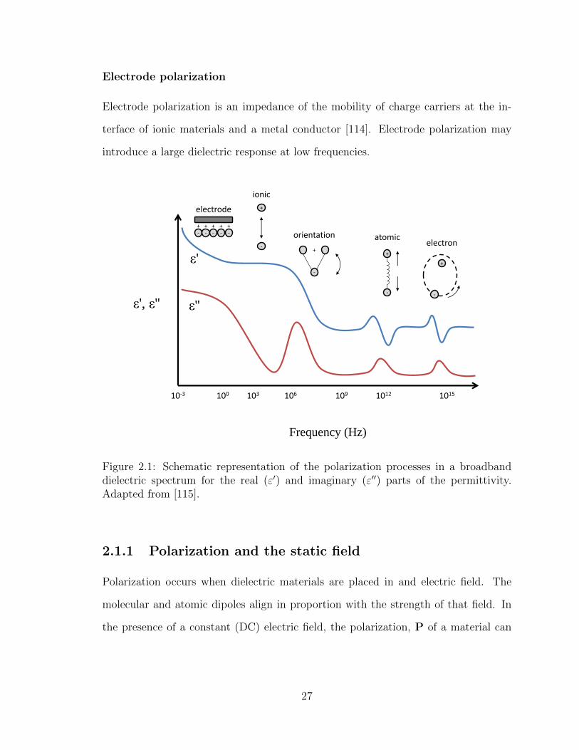
Electrode polarization
Electrode polarization is an impedance of the mobility of charge carriers at the in-
terface of ionic materials and a metal conductor [114]. Electrode polarization may
introduce a large dielectric response at low frequencies.
Frequency (Hz)
ε', ε''
+
-
+
-
-
+
+
-
ε''
ε'
electron atomic orientation
ionic
electrode
- - - - - + + + + +
1015 1012 109 106 103 100 10-3
Figure 2.1: Schematic representation of the polarization processes in a broadbanddielectric spectrum for the real (ε′) and imaginary (ε′′) parts of the permittivity.Adapted from [115].
2.1.1 Polarization and the static field
Polarization occurs when dielectric materials are placed in and electric field. The
molecular and atomic dipoles align in proportion with the strength of that field. In
the presence of a constant (DC) electric field, the polarization, P of a material can
27
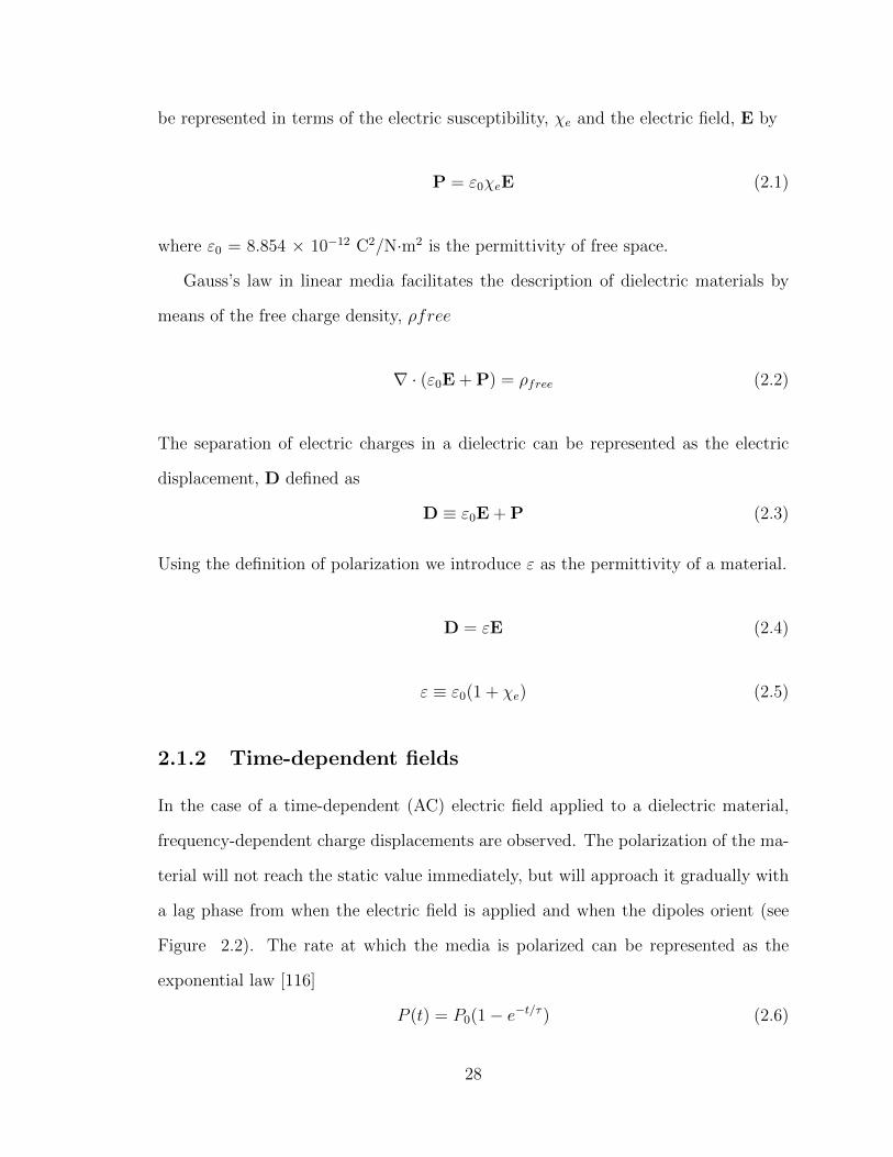
be represented in terms of the electric susceptibility, χe and the electric field, E by
P = ε0χeE (2.1)
where ε0 = 8.854 × 10⁻¹² C2/N·m2 is the permittivity of free space.
Gauss’s law in linear media facilitates the description of dielectric materials by
means of the free charge density, ρfree
∇ · (ε0E + P) = ρfree (2.2)
The separation of electric charges in a dielectric can be represented as the electric
displacement, D defined as
D ≡ ε0E + P (2.3)
Using the definition of polarization we introduce ε as the permittivity of a material.
D = εE (2.4)
ε ≡ ε0(1 + χe) (2.5)
2.1.2 Time-dependent fields
In the case of a time-dependent (AC) electric field applied to a dielectric material,
frequency-dependent charge displacements are observed. The polarization of the ma-
terial will not reach the static value immediately, but will approach it gradually with
a lag phase from when the electric field is applied and when the dipoles orient (see
Figure 2.2). The rate at which the media is polarized can be represented as the
exponential law [116]
P (t) = P0(1− e−t/τ ) (2.6)
28
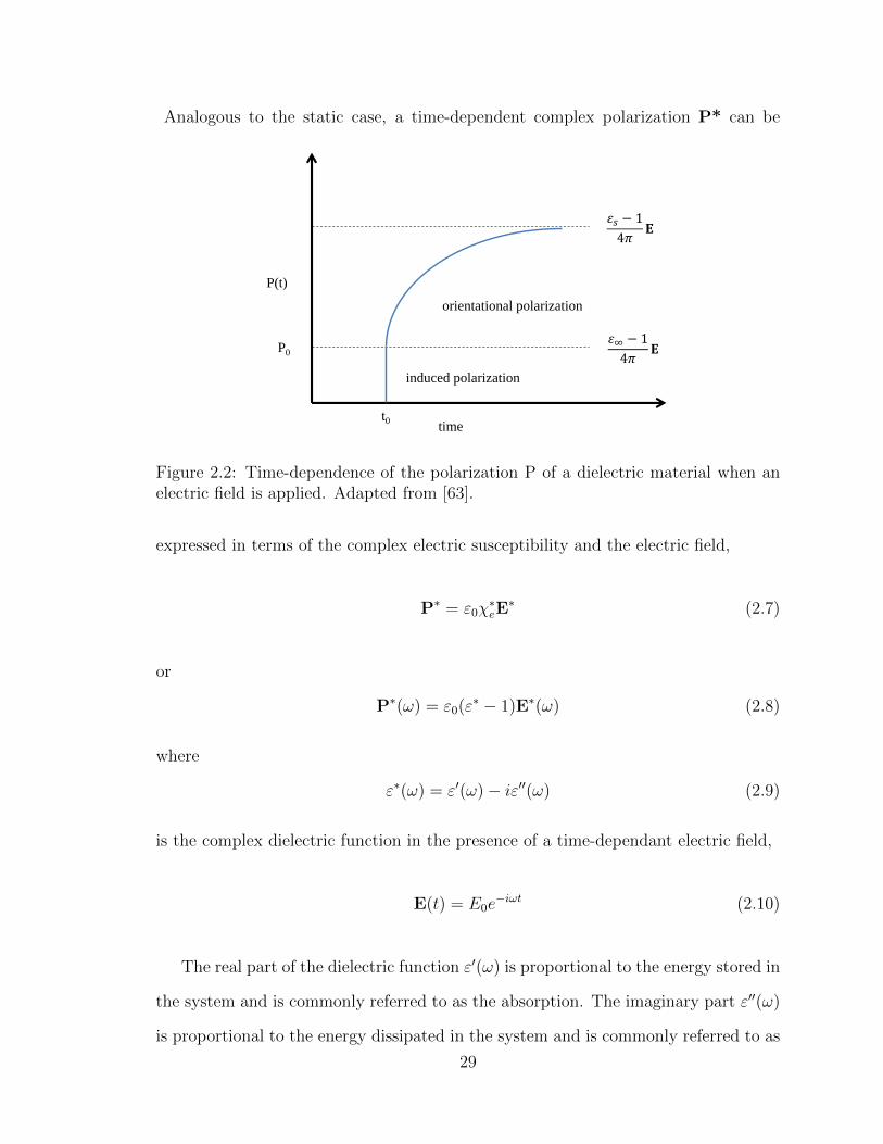
Analogous to the static case, a time-dependent complex polarization P* can be
time
P(t)
P0
𝜀𝑠 − 1
4𝜋𝐄
𝜀∞ − 1
4𝜋𝐄
induced polarization
orientational polarization
t0
Figure 2.2: Time-dependence of the polarization P of a dielectric material when anelectric field is applied. Adapted from [63].
expressed in terms of the complex electric susceptibility and the electric field,
P∗ = ε0χ∗eE∗ (2.7)
or
P∗(ω) = ε0(ε∗ − 1)E∗(ω) (2.8)
where
ε∗(ω) = ε′(ω)− iε′′(ω) (2.9)
is the complex dielectric function in the presence of a time-dependant electric field,
E(t) = E0e−iωt (2.10)
The real part of the dielectric function ε′(ω) is proportional to the energy stored in
the system and is commonly referred to as the absorption. The imaginary part ε′′(ω)
is proportional to the energy dissipated in the system and is commonly referred to as
29
the dielectric dispersion or loss [63]. The real and imaginary parts of the dielectric
function are related by the Kramers-Kronig relations [117, 63] such that
ε′(ω) = ε∞ +2
π
∫ ∞0
ξε′′(ξ)
ξ2 − ω2dξ (2.11)
ε′′(ω) = −2ω
π
∫ ∞0
ε′(ξ)− ε∞ξ2 − ω2
dξ (2.12)
where ξ is a dummy variable of integration. This relation has great significance in
practice in that the absorbtion process can be derived by observation of the disper-
sion phenomena. Application of a Laplace transformation of the polarization decay
function yields the Debye relations for dielectric relaxation [118]
ε′(ω) = ε∞ +∆ε
1 + ω2τ 2(2.13)
ε′′(ω) =∆εωτ
1 + ω2τ 2(2.14)
ε∗(ω) = ε∞ +∆ε
1 + iωτ(2.15)
where τ is the relaxation time found in P (t) = P0(1− e−t/τ ). The dielectric strength
∆ε = εs−ε∞ is introduced with the boundary conditions εs as the static permittivity
and ε∞ as the permittivity high high frequency such that
εs = ε′(0) (2.16)
ε∞ = ε′(∞) (2.17)
2.1.3 Non-Debye relaxation processes
The Debye relaxation equations assume the dielectric material is isotropic and the
decay of the polarization follows the model exponential function. Often in the case
30

of polymers and biological materials, the relaxation time is better modeled by a
non-Debye distribution. Kenneth S. Cole and Robert H. Cole first introduced a
modification of the Debye distribution with symmetric broadening of the dielectric
loss peak [119]
ε∗CC(ω) = ε∞ +∆ε
1 + (iωτCC
)β(2.18)
where β is the broadening parameter from 0< β ≤1 and τCC
is the Cole-Cole re-
laxation time. Note that when β=1, the Debye function is recovered. The maximal
dielectric loss occurs at ωmax=2πνmax=1/τCC
.
Liquids and low molecular glass-forming materials typically exhibit dielectric spec-
tra with asymmetric broadening [63]. The asymmetric broadening parameter γ,
0< γ ≤1 arises in the Davidson-Cole formalism [120, 121]
ε∗DC(ω) = ε∞ +∆ε
(1 + iωτDC
)γ(2.19)
with τDC
as the Davidson-Cole relaxation time and again, with γ=1 the Debye equa-
tions are recovered. Since the Davidson-Cole function is asymmetrical, the relaxation
time τDC
is not at the frequency of maximal dielectric loss, but rather dependent on
the shape parameters, given by [63]
ωmax =1
τDC
tan
[π
2γ + 2
](2.20)
Havriliak and Negami introduced a more general, empirical form for the relaxation
distribution to account for both symmetric and asymmetric broadening of the dielec-
tric loss [122, 123]
ε∗HN(ω) = ε∞ +∆ε
(1 + (iωτHN
)β)γ(2.21)
with τHN
as the Havriliak-Negami relaxation time. The versatility of the Havriliak-
Negami function proves to be quite useful in the analysis of anisotropic systems
31

such as polymers and biopolymers. Similar to the Davidson-Cole function, since the
Havriliak-Negami function is asymmetrical, the relaxation time τHN
is dependent on
the shape parameters, given by [63, 124]
ωmax =1
τHN
[sin
βπ
2γ + 2
]1/β [sin
βγπ
2γ + 2
]−1/β(2.22)
At low frequency, dielectric spectra are often dominated by DC conductivity due
to free ions in the solution. The conductivity only introduces dielectric loss and is
modeled by the power law
σ(ω) = −i(σ0ε0ω
)N(2.23)
where σ0 is the DC conductivity and N is the exponent of the frequency dependence
of the conductivity. In the analysis of dielectric spectra, the conductivity term is
added to a number (n) of relaxation processes such that the total dielectric function
is
ε∗(ω) = −i(σ0ε0ω
)N+
n∑k=1
[ε∞,k +
∆εk(1 + (iωτk)βk)γk
](2.24)
2.1.4 Dielectric modulus
Ionic materials, such as the case of protein-solvent mixtures, often display a highly
conductive component. In low frequency domain is often dominated by the conduc-
tivity in the region where dipole relaxation processes would be typically observed.
The dielectric modulus, M∗ is a useful parameter for analyzing the dielectric spec-
tra when ionic conductors are present [125, 126, 127, 128]. The complex modulus is
defined as:
M∗ = M ′ + iM ′′ =1
ε∗=
ε′
ε′2 + ε′′2+ i
ε′′
ε′2 + ε′′2(2.25)
32

where analogous to the permittivity, M ′ is the dielectric modulus absorbtion and M ′′
is the loss. One advantage of the dielectric modulus is that it transforms the con-
ductivity into a relaxation peak, which allows low frequency orientational relaxation
modes to be more easily studied [129].
Cole and Cole suggested a model-free method of analyzing dielectric data by plot-
ting ε′′ vs. ε′ in the complex plane [119]. Not to be confused with the Cole-Cole
dielectric function, a Cole-Cole plot can be used in the analysis of any dielectric
spectra. In the case of Debye relaxation, a perfect semicircle is obtained. Defor-
mations of the semicircle can be best modeled by the Havriliak-Negami function as
seen in Figure 2.3 where the angles of tilt are defined by the shape parameters of
the Havriliak-Negami function [63]. Each relaxation process will contribute its own
semicircle in a Cole-Cole plot and often the semicircles will overlap. Similarly in
the modulus formalism, a modulus Cole-Cole plot can be created by plotting M ′′
vs. M ′. The modulus Cole-Cole plot is particularly useful in the case of ionic liq-
uids [126, 127, 130] where the conductivity will dominate at low frequencies. Since
the conductivity appears in both M ′′ and M ′, a new semicircle for the conductivity
appears in the modulus Cole-Cole plot that is not present in the permittivity.
33
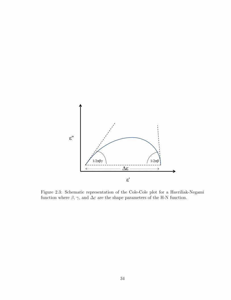
ε''
ε'
∆ε
1/2πβγ 1/2πβ
Figure 2.3: Schematic representation of the Cole-Cole plot for a Havriliak-Negamifunction where β, γ, and ∆ε are the shape parameters of the H-N function.
34
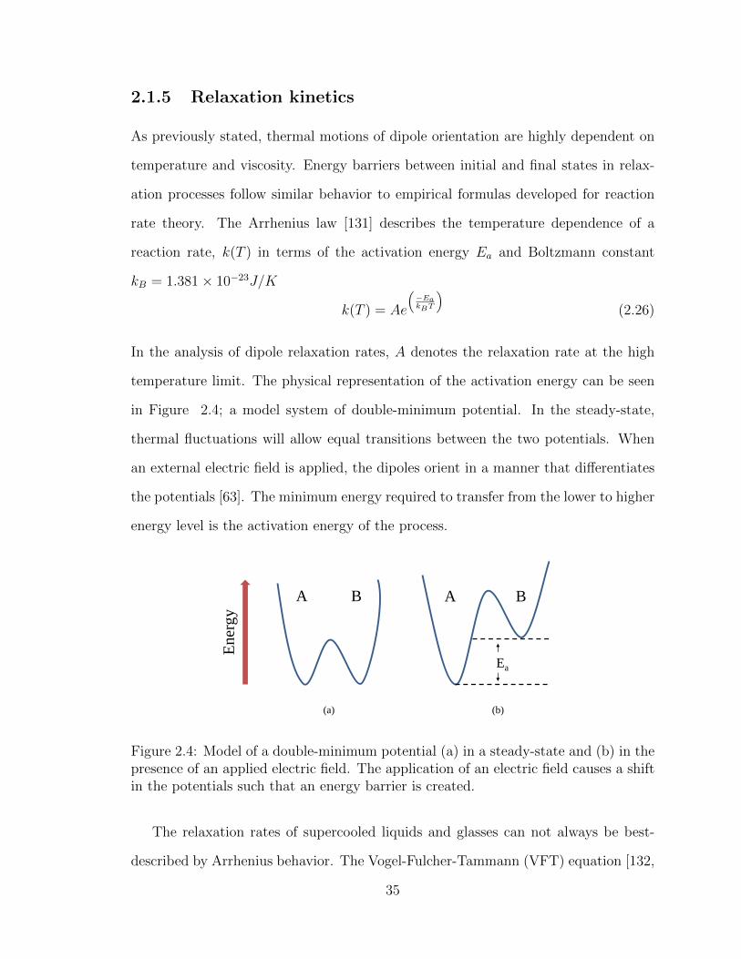
2.1.5 Relaxation kinetics
As previously stated, thermal motions of dipole orientation are highly dependent on
temperature and viscosity. Energy barriers between initial and final states in relax-
ation processes follow similar behavior to empirical formulas developed for reaction
rate theory. The Arrhenius law [131] describes the temperature dependence of a
reaction rate, k(T ) in terms of the activation energy Ea and Boltzmann constant
kB = 1.381× 10⁻²³J/K
k(T ) = Ae
(−EakBT
)(2.26)
In the analysis of dipole relaxation rates, A denotes the relaxation rate at the high
temperature limit. The physical representation of the activation energy can be seen
in Figure 2.4; a model system of double-minimum potential. In the steady-state,
thermal fluctuations will allow equal transitions between the two potentials. When
an external electric field is applied, the dipoles orient in a manner that differentiates
the potentials [63]. The minimum energy required to transfer from the lower to higher
energy level is the activation energy of the process.
A B A B
Ea
(a) (b)
Ener
gy
Figure 2.4: Model of a double-minimum potential (a) in a steady-state and (b) in thepresence of an applied electric field. The application of an electric field causes a shiftin the potentials such that an energy barrier is created.
The relaxation rates of supercooled liquids and glasses can not always be best-
described by Arrhenius behavior. The Vogel-Fulcher-Tammann (VFT) equation [132,
35
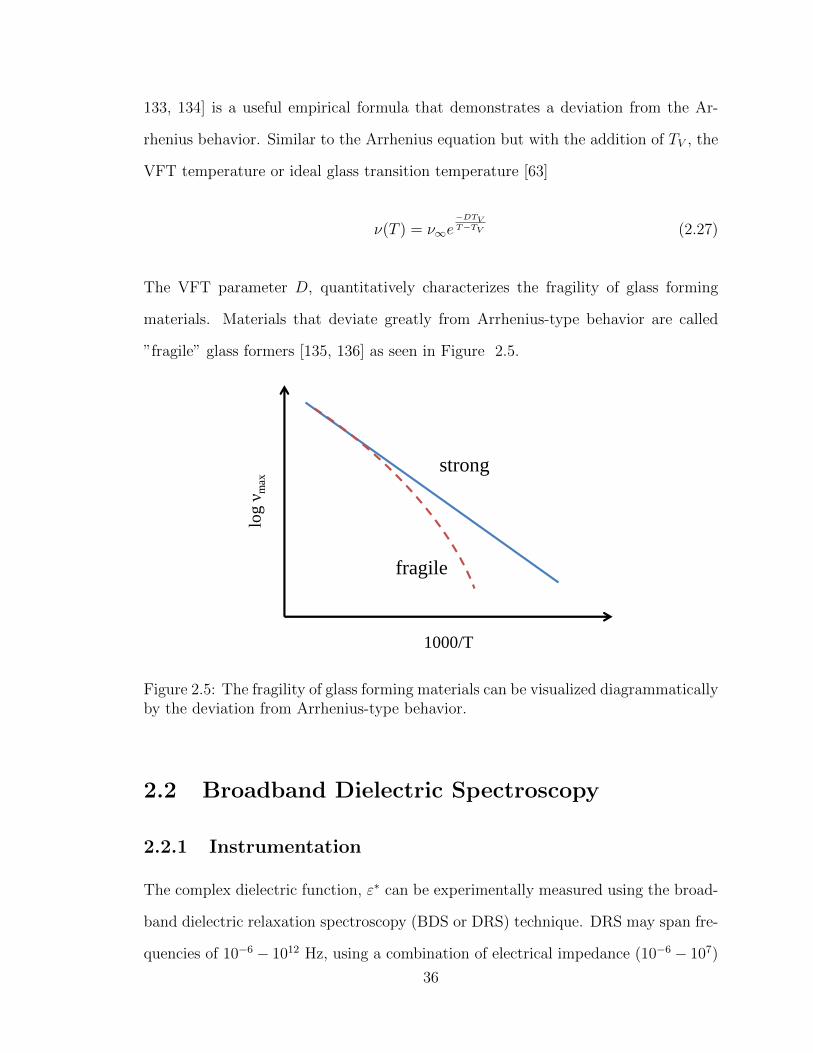
133, 134] is a useful empirical formula that demonstrates a deviation from the Ar-
rhenius behavior. Similar to the Arrhenius equation but with the addition of TV , the
VFT temperature or ideal glass transition temperature [63]
ν(T ) = ν∞e−DTVT−TV (2.27)
The VFT parameter D, quantitatively characterizes the fragility of glass forming
materials. Materials that deviate greatly from Arrhenius-type behavior are called
”fragile” glass formers [135, 136] as seen in Figure 2.5.
1000/T
log ν
max
strong
fragile
Figure 2.5: The fragility of glass forming materials can be visualized diagrammaticallyby the deviation from Arrhenius-type behavior.
2.2 Broadband Dielectric Spectroscopy
2.2.1 Instrumentation
The complex dielectric function, ε∗ can be experimentally measured using the broad-
band dielectric relaxation spectroscopy (BDS or DRS) technique. DRS may span fre-
quencies of 10−6 − 1012 Hz, using a combination of electrical impedance (10−6 − 107)
36

and optical measurement 107 − 1012 techniques [63]. Our measurements are limited
to electrical impedance in which the sample is treated as a parallel or serial circuit of
an ideal capacitor and ohmic resistor.
In DRS, a capacitive sample cell made of two conducting parallel plates is place
under a probing AC field with a fixed frequency, V0. When a dielectric sample is
placed between the two plates, the capacitance increases over that of the empty
cell. The dielectric permittivity can be directly measured by relating the empty cell
capacitance to the capacitance in the presence of a sample. When a voltage is applied
to a dielectric sample, the dipoles will align as in Figure 2.6.
+ + + + + + + +
- - - - - - - - +
-
+
-
+
-
+
-
+
-
+
-
+
-
+
-
+
-
+
-
+
-
+
-
+
-
+
-
+
-
+
-
+
Figure 2.6: Material dipoles are typically in a random orientation. When placedinside an electric field, the dipoles align between the capacitive plates.
The applied voltage results in an induced current, I0 at the same frequency with
a phase shift, ϕ shown in Figure 2.7.
For a capacitor filled with a sample, the complex dielectric permittivity, ε∗ is
defined as the ratio,
ε∗ = ε′(ω)− iε′′(ω) =C∗
C0
(2.28)
where C∗(ω) is the complex capacitance and C0 is the empty cell (vacuum) capaci-
tance [63]. When an oscillating AC field, V ∗(ω) = V0eiωt, the dielectric function can
37
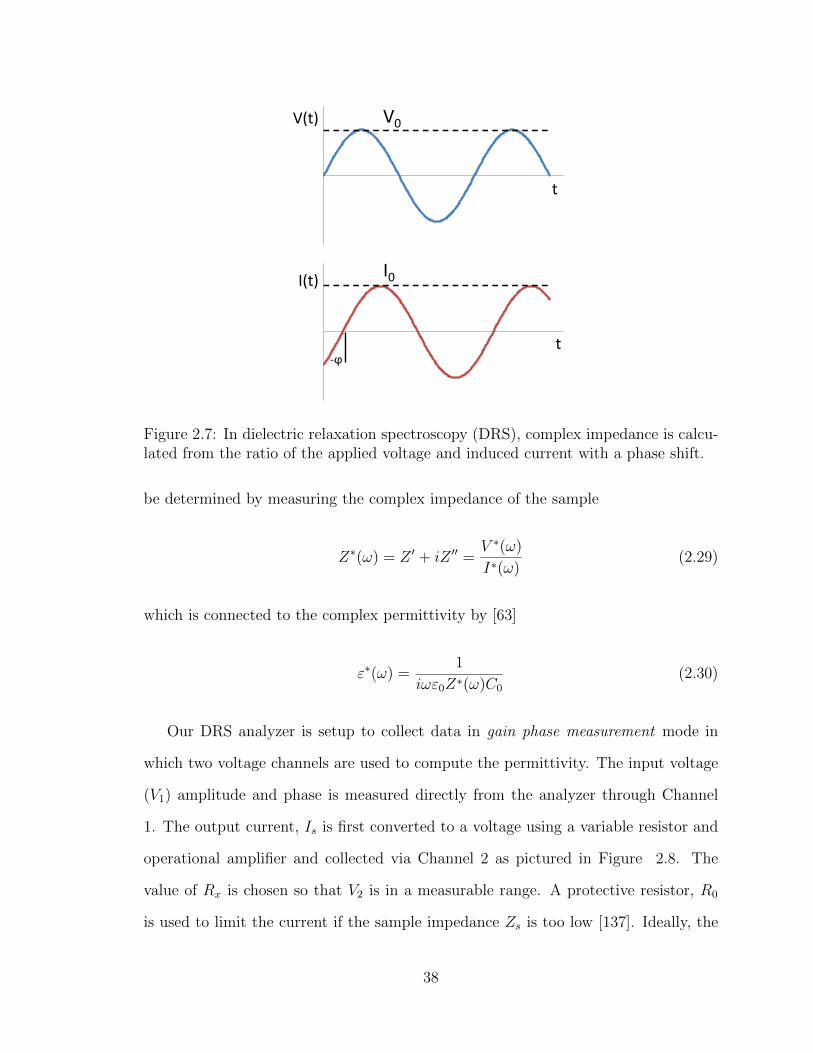
t
V(t) V0
I(t)
t
I0
-ϕ
Figure 2.7: In dielectric relaxation spectroscopy (DRS), complex impedance is calcu-lated from the ratio of the applied voltage and induced current with a phase shift.
be determined by measuring the complex impedance of the sample
Z∗(ω) = Z ′ + iZ ′′ =V ∗(ω)
I∗(ω)(2.29)
which is connected to the complex permittivity by [63]
ε∗(ω) =1
iωε0Z∗(ω)C0
(2.30)
Our DRS analyzer is setup to collect data in gain phase measurement mode in
which two voltage channels are used to compute the permittivity. The input voltage
(V1) amplitude and phase is measured directly from the analyzer through Channel
1. The output current, Is is first converted to a voltage using a variable resistor and
operational amplifier and collected via Channel 2 as pictured in Figure 2.8. The
value of Rx is chosen so that V2 is in a measurable range. A protective resistor, R0
is used to limit the current if the sample impedance Zs is too low [137]. Ideally, the
38
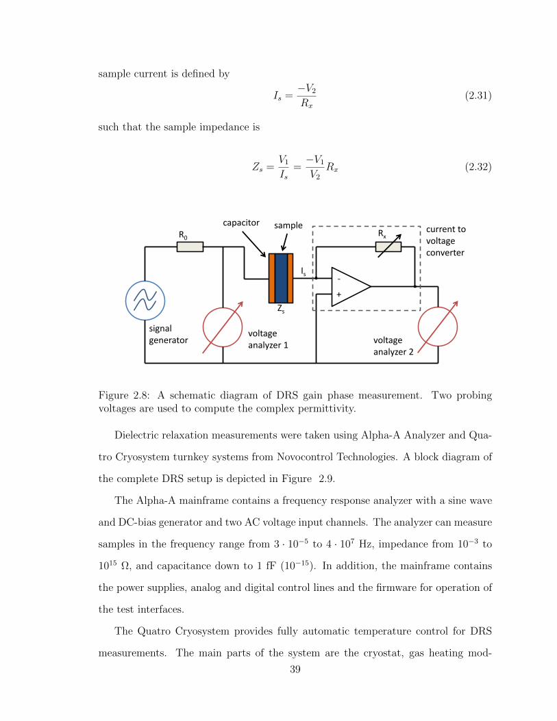
sample current is defined by
Is =−V2Rx
(2.31)
such that the sample impedance is
Zs =V1Is
=−V1V2
Rx (2.32)
signal generator
voltage analyzer 1
voltage analyzer 2
capacitor sample
+
-
current to voltage converter
R0 Rx
Is
Zs
Figure 2.8: A schematic diagram of DRS gain phase measurement. Two probingvoltages are used to compute the complex permittivity.
Dielectric relaxation measurements were taken using Alpha-A Analyzer and Qua-
tro Cryosystem turnkey systems from Novocontrol Technologies. A block diagram of
the complete DRS setup is depicted in Figure 2.9.
The Alpha-A mainframe contains a frequency response analyzer with a sine wave
and DC-bias generator and two AC voltage input channels. The analyzer can measure
samples in the frequency range from 3 · 10−5 to 4 · 107 Hz, impedance from 10−3 to
1015 Ω, and capacitance down to 1 fF (10−15). In addition, the mainframe contains
the power supplies, analog and digital control lines and the firmware for operation of
the test interfaces.
The Quatro Cryosystem provides fully automatic temperature control for DRS
measurements. The main parts of the system are the cryostat, gas heating mod-
39

Alpha-A analyzer
power supply
Quatro controller PC with WinDETA
cryostat
N2 dewar
liquid nitrogen evaporator
vaporizing module
Gas heating module
Figure 2.9: Block diagram of the Novocontrol Broadband Dielectric/Impedance Spec-trometer apparatus with the Alpha-A analyzer and Quatro Cryosystem.
ule, pressurizer module, vacuum system, liquid nitrogen dewar, controller and power
supply. The Quatro controller has four circuits controlling sample temperature, gas
temperature, liquid nitrogen temperature in the dewar, and pressure in the dewar.
The temperature control range is from −160C to 400C with 0.01C temperature
stability.
2.2.2 Sample cells
The Novocontrol BDS 1309 and 1307 sample cells were used to obtain DRS mea-
surements. The BDS 1309 cylindrical gold-plated cell is optimal for use with liquids
of high permittivity and ion DC conductivity. The cell geometry is designed such
that electrode spacing is unusually wide and approximately equal to the electrode
diameter. This seeks to combat high sample capacity and low frequency electrode
40
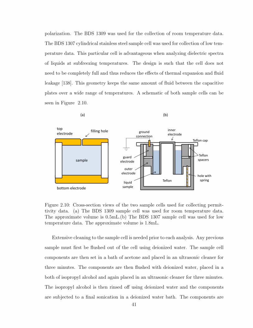
polarization. The BDS 1309 was used for the collection of room temperature data.
The BDS 1307 cylindrical stainless steel sample cell was used for collection of low tem-
perature data. This particular cell is advantageous when analyzing dielectric spectra
of liquids at subfreezing temperatures. The design is such that the cell does not
need to be completely full and thus reduces the effects of thermal expansion and fluid
leakage [138]. This geometry keeps the same amount of fluid between the capacitive
plates over a wide range of temperatures. A schematic of both sample cells can be
seen in Figure 2.10.
top electrode
bottom electrode
sample
filling hole inner electrode
Teflon liquid
sample
outer electrode
guard electrode
ground connection
Teflon spacers
Teflon cap
hole with spring
(a) (b)
Figure 2.10: Cross-section views of the two sample cells used for collecting permit-tivity data. (a) The BDS 1309 sample cell was used for room temperature data.The approximate volume is 0.5mL.(b) The BDS 1307 sample cell was used for lowtemperature data. The approximate volume is 1.8mL.
Extensive cleaning to the sample cell is needed prior to each analysis. Any previous
sample must first be flushed out of the cell using deionized water. The sample cell
components are then set in a bath of acetone and placed in an ultrasonic cleaner for
three minutes. The components are then flushed with deionized water, placed in a
both of isopropyl alcohol and again placed in an ultrasonic cleaner for three minutes.
The isopropyl alcohol is then rinsed off using deionized water and the components
are subjected to a final sonication in a deionized water bath. The components are
41

rinsed a final time in deionized water. The stainless steel pieces are placed in an oven
at 350F for approximately five minutes and the Teflon pieces are set on the bench
to air dry. The parts are allowed to cool to room temperature prior to placing any
sample in the cell.
2.3 Data Analysis Methods
The data was collected using a PC and the Novocontrol WinDETA software pack-
age. WinDETA is a system control package for experimental setup, data evaluation
and graphical representation in two or three dimensional diagrams. The measured
impedance data is used to calculate basic dielectric and impedance parameters, such
as complex dielectric function, modulus, and conductivity. The calibration procedure
for the sample cells is done automatically using a set of input parameters provided
by Novocontrol. Worklists are created to collect data as a function of frequency and
temperature. ASCII files for each measurement can be exported for external analysis
of the impedance data.
Data analysis and curve fitting was done using the WinFIT program from Novo-
control. In the frequency domain, WinFIT is used to optimize best-fit curves of di-
electric data using Debye, Cole-Cole, Cole-Davidson, and Havriliak-Negami functions
and conductivity. Up to three relaxation processes can be simultaneously optimized.
In the temperature domain, the peak relaxation times can be modeled using the
Vogel-Fulcher-Tammann (VFT) function and displayed in an Arrhenius plot. Activa-
tion energies and glass-forming fragilities for each relaxation process are determined
by fits to the VFT or Arrhenius plots.
Further curve fitting and plotting was done using Igor Pro 6 from WaveMet-
rics. Igor Pro can perform mean square deviation (MSD) minimization of user-
42

defined curve fitting functions. General text files of dielectric data was exported
using WinDETA, then imported into Igor Pro for additional analysis and plotting.
Fitting procedure
Curve fitting of the dielectric permittivity data was done in the frequency domain
using the WinFIT program. Two Havriliak-Negami functions with a conductivity tail
were chosen as fit functions to analyze the imaginary part of the permittivity, ε′′ in a
log-log representation. Figure 2.11 shows an example total fit with the deconvolution
of the three fit functions and experimental data.
The fitting procedure begins with a visual estimate of the conductivity, τ , and
∆ε parameters. A least squares fit is then done by WinFIT to optimize the conduc-
tivity, then τ and ∆ε for both Havriliak-Negami functions, simultaneously. Often
the onductivity must then be re-optimized once the τ and ∆ε have been fixed. The
spread parameters of the Havriliak-Negami function, β and γ are then optimized, if
symmetric or asymmetric broadening are observed. The high frequency permittivity
limit, ε∞ can then be optimized by analyzing the real part of the permittivity, ε′,
though this parameter is not needed for further analysis. This process is repeated
to fit dielectric spectra for each temperature point. At temperatures below approxi-
mately 200K, a linear-log plot of ε′′ versus frequency is also used for optimization of
Havriliak-Negami parameters.
The activation energies and glass-forming fragilities can be modeled by utilizing
the fits to the permittivity data over a broad range of temperatures. The maximum
frequency for each relaxation process, fmax is plotted versus inverse temperature,
1000/T as shown in Figure 2.12. The maximum frequency of each relaxation process
is related to the relaxation time by τmax = 1/(2πfmax). The log fmax vs. 1000/T plot
for each relaxation process is then fitted using either an Arrhenius (linear) or VFT
(curved) fit function.
43
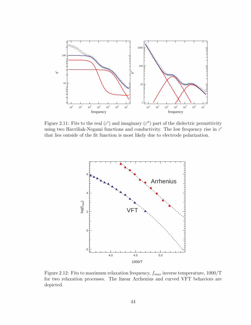
2
3
4
567
10
2
3
4
567
100
2
3
ε'
101
102
103
104
105
106
107
frequency
1
10
100
1000
ε''
101
102
103
104
105
106
107
frequency
Figure 2.11: Fits to the real (ε′) and imaginary (ε′′) part of the dielectric permittivityusing two Havriliak-Negami functions and conductivity. The low frequency rise in ε′
that lies outside of the fit function is most likely due to electrode polarization.
6
4
2
0
-2
log(
f max
)
5.04.54.0
1000/T
VFT
Arrhenius
Figure 2.12: Fits to maximum relaxation frequency, fmax inverse temperature, 1000/Tfor two relaxation processes. The linear Arrhenius and curved VFT behaviors aredepicted.
44
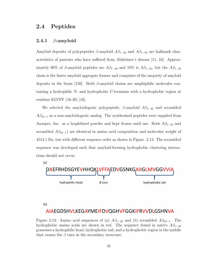
2.4 Peptides
2.4.1 β-amyloid
Amyloid deposits of polypeptides β-amyloid Aβ1−42 and Aβ1−40 are hallmark char-
acteristics of patients who have suffered from Alzheimer’s disease [11, 10]. Approx-
imately 90% of β-amyloid peptides are Aβ1−40 and 10% is Aβ1−42, but the Aβ1−42
chain is the faster amyloid aggregate former and comprises of the majority of amyloid
deposits in the brain [139]. Both β-amyloid chains are amphiphilic molecules con-
taining a hydrophilic N- and hydrophobic C-terminus with a hydrophobic region at
residues KLVFF (16-20) [16].
We selected the amyloidogenic polypeptide, β-amyloid Aβ1−42 and scrambled
Aβ42−1 as a non-amyloidogenic analog. The synthesized peptides were supplied from
Anaspec, Inc. as a lyophilized powder and kept frozen until use. Both Aβ1−42 and
scrambled Aβ42−1) are identical in amino acid composition and molecular weight of
4514.1 Da, but with different sequence order as shown in Figure 2.13. The scrambled
sequence was developed such that amyloid-forming hydrophobic clustering interac-
tions should not occur.
DAEFRHDSGYEVHHQKLVFFAEDVGSNKGAIIGLMVGGVVIA
hydrophilic head β turn hydrophobic tail
(a)
AIAEGDSHVLKEGAYMEIFDVQGHVFGGKIFRVVDLGSHNVA
(b)
Figure 2.13: Amino acid sequences of (a) Aβ1−42 and (b) scrambled Aβ42−1. Thehydrophobic amino acids are shown in red. The sequence found in native Aβ1−42possesses a hydrophilic head, hydrophobic tail, and a hydrophobic region in the middlethat causes the β turn in the secondary structure.
45
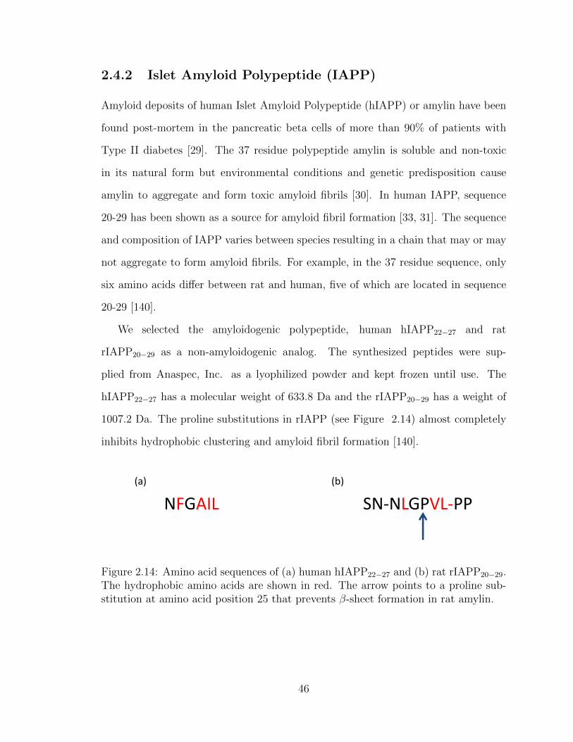
2.4.2 Islet Amyloid Polypeptide (IAPP)
Amyloid deposits of human Islet Amyloid Polypeptide (hIAPP) or amylin have been
found post-mortem in the pancreatic beta cells of more than 90% of patients with
Type II diabetes [29]. The 37 residue polypeptide amylin is soluble and non-toxic
in its natural form but environmental conditions and genetic predisposition cause
amylin to aggregate and form toxic amyloid fibrils [30]. In human IAPP, sequence
20-29 has been shown as a source for amyloid fibril formation [33, 31]. The sequence
and composition of IAPP varies between species resulting in a chain that may or may
not aggregate to form amyloid fibrils. For example, in the 37 residue sequence, only
six amino acids differ between rat and human, five of which are located in sequence
20-29 [140].
We selected the amyloidogenic polypeptide, human hIAPP22−27 and rat
rIAPP20−29 as a non-amyloidogenic analog. The synthesized peptides were sup-
plied from Anaspec, Inc. as a lyophilized powder and kept frozen until use. The
hIAPP22−27 has a molecular weight of 633.8 Da and the rIAPP20−29 has a weight of
1007.2 Da. The proline substitutions in rIAPP (see Figure 2.14) almost completely
inhibits hydrophobic clustering and amyloid fibril formation [140].
SN-NLGPVL-PP
(b)(a)
NFGAIL
Figure 2.14: Amino acid sequences of (a) human hIAPP22−27 and (b) rat rIAPP20−29.The hydrophobic amino acids are shown in red. The arrow points to a proline sub-stitution at amino acid position 25 that prevents β-sheet formation in rat amylin.
46
2.5 Buffers
Experiments were performed using a deionized water or bovine serum albumin (BSA)
buffer. The deionized water, 18.2MΩ·cm minimum, was supplied using a Millipore
Direct-Q water purification system. The BSA was purchased from Sigma, cata-
logue #B8655 with a protein concentration of 45-75 mg/mL and containing 0.01%
thimerosal as a preservative. The serum was kept frozen until use. Glycerol, 99%
minimum (Sigma, #G5516) was used as a cryoprotectant for experiments under sub-
freezing temperatures.
47
Chapter 3
Dielectric Studies of
Amyloidogenic Peptides at Room
Temperature as a Function of
Concentration and Incubation
Time
3.1 Overview
Amyloidogenic peptides characteristically aggregate to form higher-ordered structures
from dimers, trimers, and oliogomers, to protofibrils and fibrillar plaques [44, 45, 46,
47]. Aggregation and changes to the surface landscape of amyloid structures produces
a redistribution of mobile charge carriers and molecular dipoles. This redistribution
is reflected in a changing dielectric response over time during the fibrillation process.
The aim of our work was to characterize the dielectric relaxation response for two
amyloidogenic peptides and their non-amyloidogenic analogs. Amyloidogenic pep-
48

tides Aβ1−42 and human islet amyloid polypeptide, hIAPP22−27 were used as mod-
els for studying protein aggregation and beta sheet formation at room temperature.
Their non-amyloidogenic analogs, scrambled Aβ42−1 and rat islet amyloid polypep-
tide, rIAPP20−29 were selected as control materials. Dielectric measurements at room
temperature of conductive, heterogeneous materials, such as proteins, are dominated
by conductivity and polarization effects [127, 126]. Here, we explore changes to con-
ductivity and space-charge polarization as amyloidogenic peptides combine to form
higher-ordered structures.
3.2 Sample Preparation and Data Collection
Lyophilized peptides of Aβ1−42, scrambled Aβ42−1, hIAPP22−27, rIAPP20−29 were ob-
tained from AnaSpec, Inc in quantities of 0.5 mg and 1.0 mg. The vials were stored at
approximately -20C until the time of reconstitution. The Aβ1−42 was first rehydrated
using 35µL 1% NH4OH added to 0.5mg of protein to ensure that the solution was first
driven to a monomeric state. Deionized water, 18.2MΩ·cm minimum, was used to
dilute and rehydrate the peptides to concentrations of 5µM, 50µM, and 100µM. Each
solution was stored in sterile vials. The samples were then mixed by repeated inver-
sion of the vials and set to incubate for 0-168 hours at room temperature. The same
sample preparation was used for each time point. The samples were again mixed by
repeated inversion of the vials, then placed in the Novocontrol BDS 1309 cylindrical
gold-plated sample cell.
Data were collected using the Novocontrol Alpha-A Analyzer and Quatro Cryosys-
tem in gain phase measurement mode with an AC probing voltage of 1.000 VRMS.
Measurements were taken at room temperature of approximately 295 K. We selected
60 data points in a frequency range from 1.00× 10⁷ − 4.78× 10⁻² Hz, spaced evenly
in a logarithmic scale.
49
3.3 Results and Discussions
3.3.1 Studies of Aβ1−42 and Scrambled Aβ42−1
The dielectric spectra of Aβ1−42 and scrambled Aβ42−1 at concentrations of 5µM,
50µM, and 100µM are presented at various incubation times in Figures 3.2 - 3.4.
Dielectric spectra are typically represented using the permittivity formalism, however
interfacial polarization and DC conductivity dominate the spectra in the case of highly
conductive materials. The interfacial polarization occurs due to the space-charge ac-
cumulation at macroscopic interfaces as a result of the differences in conductivities
and permittivities in heterogenous materials [126]. The dielectric modulus is an alter-
native formalism used to study the conductivity and relaxation spectra of materials
in the presence of interfacial polarization [125, 126, 127, 128]. Figure 3.1 shows the
relationship between M ′′, ε′, and ε′′. When plotted together, the intersection of ε′
and ε′′ occurs at the peak loss modulus, M ′′ for the conductivity. The region of ε′
with zero slope is the conductivity and the region of negative slope is polarization
effects. In the following, we present the dielectric spectra using the dielectric loss
modulus, M ′′ as a function of frequency to show the changes in the conductivity
process throughout fibril formation.
50
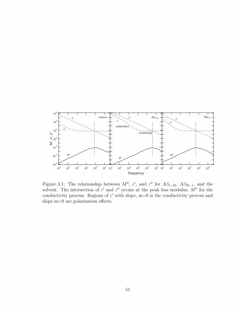
101
102
103
104
105
106
frequency
Aβ1-42
10-6
10-4
10-2
100
102
104
106
M'',
ε',
ε''
101
102
103
104
105
106
solvent
101
102
103
104
105
106
Aβ42-1
M''
ε'
ε''ε'
ε'
ε'' ε''
M''M''
conductivity
polarization
Figure 3.1: The relationship between M ′′, ε′, and ε′′ for Aβ1−42, Aβ42−1, and thesolvent. The intersection of ε′ and ε′′ occurs at the peak loss modulus, M ′′ for theconductivity process. Regions of ε′ with slope, m=0 is the conductivity process andslope m<0 are polarization effects.
51

10x10-3
8
6
4
2
M''
103
104
105
106
107
frequency
Aβ1-42 1 hr 5µM 50µM 100µM solvent
10x10-3
8
6
4
2
M''
103
104
105
106
107
frequency
Aβ1-42 4 hr 5µM 50µM 100µM solvent
103
104
105
106
107
frequency
Aβ42-1 4 hr 5µM 50µM 100µM solvent
103
104
105
106
107
frequency
Aβ42-1 1 hr 5µM 50µM 100µM solvent
2 decades
1.5 decades
1 decade
0.5 decade
2 decades
0.5 decade
Figure 3.2: Dielectric modulus (M ′′) as a function of frequency for Aβ1−42and Aβ42−1 at concentrations of 5µM, 50µM and 100µM after 1 hour and4 hours of incubation time. There is an immediate shift in peak frequency forAβ1−42 for all concentrations after just 1 hour. The peak shift for Aβ42−1 is only ahalf decade or less for both 1 and 4 hours for all concentrations. Note that after 4hours of incubation, the shift for 5µM Aβ1−42 is more than twice the shift for anyconcentration of Aβ42−1.
52
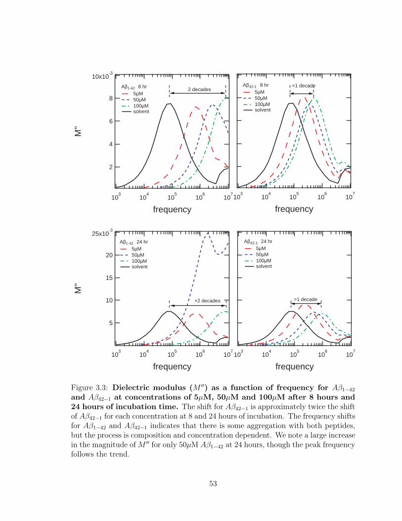
10x10-3
8
6
4
2
M''
103
104
105
106
107
frequency
Aβ1-42 8 hr 5µM 50µM 100µM solvent
103
104
105
106
107
frequency
Aβ42-1 8 hr 5µM 50µM 100µM solvent
25x10-3
20
15
10
5
M''
103
104
105
106
107
frequency
Aβ1-42 24 hr 5µM 50µM 100µM solvent
103
104
105
106
107
frequency
Aβ42-1 24 hr 5µM 50µM 100µM solvent
2 decades<1 decade
+2 decades >1 decade
Figure 3.3: Dielectric modulus (M ′′) as a function of frequency for Aβ1−42and Aβ42−1 at concentrations of 5µM, 50µM and 100µM after 8 hours and24 hours of incubation time. The shift for Aβ42−1 is approximately twice the shiftof Aβ42−1 for each concentration at 8 and 24 hours of incubation. The frequency shiftsfor Aβ1−42 and Aβ42−1 indicates that there is some aggregation with both peptides,but the process is composition and concentration dependent. We note a large increasein the magnitude of M ′′ for only 50µM Aβ1−42 at 24 hours, though the peak frequencyfollows the trend.
53

14x10-3
12
10
8
6
4
2
M''
103
104
105
106
107
frequency
Aβ1-42 72 hr 5µM 50µM 100µM solvent
103
104
105
106
107
frequency
Aβ42-1 72 hr 5µM 50µM 100µM solvent
10x10-3
8
6
4
2
M"
103
104
105
106
107
frequency
Aβ1-42 144 hr 5µM 50µM
solvent
103
104
105
106
107
frequency
Aβ42-1 144 hr 5µM 50µM 100µM solvent
1 decade 1.5 decades
1.5 decades >1 decade
Figure 3.4: Dielectric modulus (M ′′) as a function of frequency for Aβ1−42and Aβ42−1 at concentrations of 5µM, 50µM and 100µM after 72 hours and144 hours of incubation time. The shift for Aβ42−1 is approximately 1.5 timesthe shift of Aβ42−1 for each concentration at 72 and 144 hours of incubation. We notea large increase in the magnitude of M ′′ for 100µM Aβ1−42 at 72 hours, though thepeak frequency follows the trend to higher frequency. Data was not collected beyond72 hours for Aβ1−42.
54
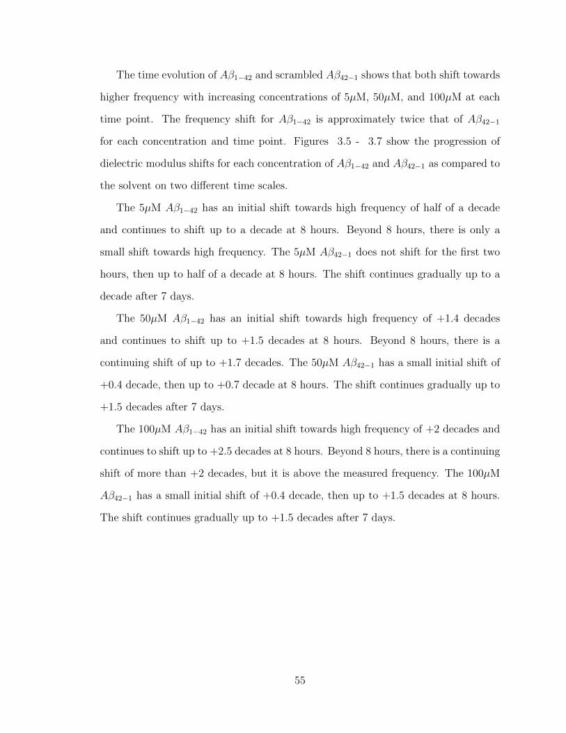
The time evolution of Aβ1−42 and scrambled Aβ42−1 shows that both shift towards
higher frequency with increasing concentrations of 5µM, 50µM, and 100µM at each
time point. The frequency shift for Aβ1−42 is approximately twice that of Aβ42−1
for each concentration and time point. Figures 3.5 - 3.7 show the progression of
dielectric modulus shifts for each concentration of Aβ1−42 and Aβ42−1 as compared to
the solvent on two different time scales.
The 5µM Aβ1−42 has an initial shift towards high frequency of half of a decade
and continues to shift up to a decade at 8 hours. Beyond 8 hours, there is only a
small shift towards high frequency. The 5µM Aβ42−1 does not shift for the first two
hours, then up to half of a decade at 8 hours. The shift continues gradually up to a
decade after 7 days.
The 50µM Aβ1−42 has an initial shift towards high frequency of +1.4 decades
and continues to shift up to +1.5 decades at 8 hours. Beyond 8 hours, there is a
continuing shift of up to +1.7 decades. The 50µM Aβ42−1 has a small initial shift of
+0.4 decade, then up to +0.7 decade at 8 hours. The shift continues gradually up to
+1.5 decades after 7 days.
The 100µM Aβ1−42 has an initial shift towards high frequency of +2 decades and
continues to shift up to +2.5 decades at 8 hours. Beyond 8 hours, there is a continuing
shift of more than +2 decades, but it is above the measured frequency. The 100µM
Aβ42−1 has a small initial shift of +0.4 decade, then up to +1.5 decades at 8 hours.
The shift continues gradually up to +1.5 decades after 7 days.
55

14x10-3
12
10
8
6
4
2
M''
103
104
105
106
107
frequency
Aβ1-42 5µM 1 hr 168 hr 24 hr solvent 72 hr
103
104
105
106
107
frequency
Aβ42-1 5µM 1 hr 168 hr 24 hr solvent 72 hr
14x10-3
12
10
8
6
4
2
M''
103
104
105
106
107
frequency
Aβ1-42 5µM 0 hr 4 hr 1 hr 8hr 2 hr solvent
103
104
105
106
107
frequency
Aβ42-1 5µM 0 hr 4 hr 1 hr 8hr 2 hr solvent
Figure 3.5: Time evolution for 5 µM Aβ1−42 and Aβ42−1 for 0-8 hours and1-168 hours (7 days). The Aβ1−42 has an initial jump in peak frequency of approx-imately 1 decade at the first measurement, then continues for another half decade.There is no shift in Aβ24−1 for the first two hours, then steady shift throughout 168hours. The peak frequencies of Aβ1−42 and Aβ42−1 are very close after 168 hours ofincubation.
56

25x10-3
20
15
10
5
M''
103
104
105
106
107
frequency
Aβ1-42 50µM 1 hr 168 hr 24 hr solvent 72 hr
103
104
105
106
107
frequency
Aβ42-1 50µM 1 hr 168 hr 24 hr solvent 72 hr
103
104
105
106
107
frequency
Aβ42-1 50µM 0 hr 4 hr 1 hr 8hr 2 hr solvent
14x10-3
12
10
8
6
4
2
M''
103
104
105
106
107
frequency
Aβ1-42 50µM 0 hr 4 hr 1 hr 8hr 2 hr solvent
Figure 3.6: Time evolution for 50 µM Aβ1−42 and Aβ42−1 for 0-8 hours and1-168 hours (7 days). The Aβ1−42 has an initial jump in peak frequency of approx-imately 1.5 decades at the first measurement, then continues with small increases.There is a small shift in Aβ24−1 of a half decade, then steady shift throughout 168hours. The peak frequency of Aβ1−42 is approximately a half decade above Aβ42−1after 168 hours of incubation. The large increase in the magnitude of Aβ1−42 at 0 and24 hours could be the result of an evolving surface landscape during fibril formation.
57
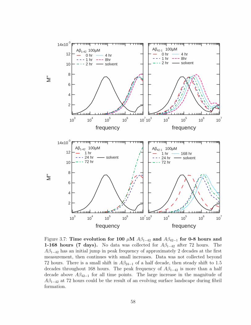
103
104
105
106
107
frequency
Aβ42-1 100µM 0 hr 4 hr 1 hr 8hr 2 hr solvent
14x10-3
12
10
8
6
4
2
M''
103
104
105
106
107
frequency
Aβ1-42 100µM 0 hr 4 hr 1 hr 8hr 2 hr solvent
103
104
105
106
107
frequency
Aβ42-1 100µM 1 hr 168 hr 24 hr solvent 72 hr
14x10-3
12
10
8
6
4
2
M''
103
104
105
106
107
frequency
Aβ1-42 100µM 1 hr 24 hr solvent 72 hr
Figure 3.7: Time evolution for 100 µM Aβ1−42 and Aβ42−1 for 0-8 hours and1-168 hours (7 days). No data was collected for Aβ1−42 after 72 hours. TheAβ1−42 has an initial jump in peak frequency of approximately 2 decades at the firstmeasurement, then continues with small increases. Data was not collected beyond72 hours. There is a small shift in Aβ24−1 of a half decade, then steady shift to 1.5decades throughout 168 hours. The peak frequency of Aβ1−42 is more than a halfdecade above Aβ42−1 for all time points. The large increase in the magnitude ofAβ1−42 at 72 hours could be the result of an evolving surface landscape during fibrilformation.
58
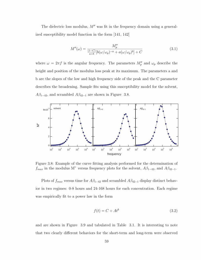
The dielectric loss modulus, M ′′ was fit in the frequency domain using a general-
ized susceptibility model function in the form [141, 142]
M ′′(ω) =M ′′
p
(1−C)a+b
[b(ω/ωp)−a + a(ω/ωp)b] + C(3.1)
where ω = 2πf is the angular frequency. The parameters M ′′p and ωp describe the
height and position of the modulus loss peak at its maximum. The parameters a and
b are the slopes of the low and high frequency side of the peak and the C parameter
describes the broadening. Sample fits using this susceptibility model for the solvent,
Aβ1−42, and scrambled Aβ42−1 are shown in Figure 3.8.
102
103
104
105
106
frequency
102
103
104
105
106
8x10⁻³
6
4
2
0
M"
102
103
104
105
106
solvent Aβ1-42 Aβ42-1
Figure 3.8: Example of the curve fitting analysis performed for the determination offmax in the modulus M” versus frequency plots for the solvent, Aβ1−42, and Aβ42−1.
Plots of fmax versus time for Aβ1−42 and scrambled Aβ42−1 display distinct behav-
ior in two regimes: 0-8 hours and 24-168 hours for each concentration. Each regime
was empirically fit to a power law in the form
f(t) = C + Atk (3.2)
and are shown in Figure 3.9 and tabulated in Table 3.1. It is interesting to note
that two clearly different behaviors for the short-term and long-term were observed
59
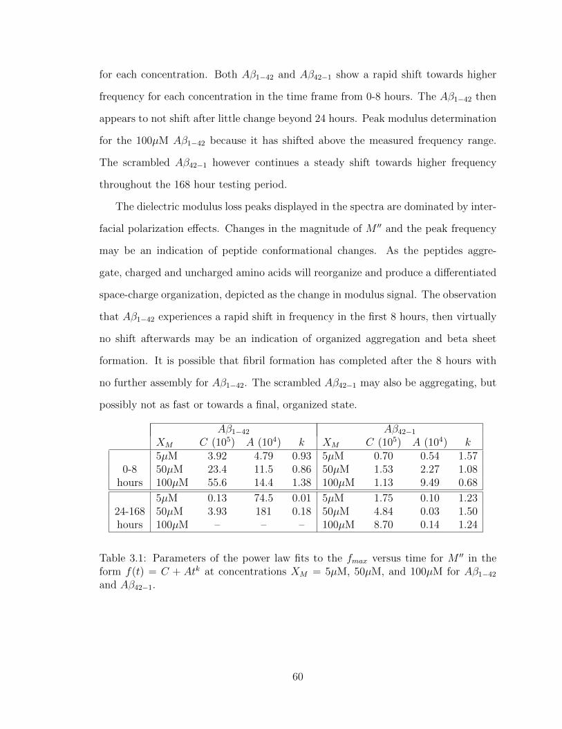
for each concentration. Both Aβ1−42 and Aβ42−1 show a rapid shift towards higher
frequency for each concentration in the time frame from 0-8 hours. The Aβ1−42 then
appears to not shift after little change beyond 24 hours. Peak modulus determination
for the 100µM Aβ1−42 because it has shifted above the measured frequency range.
The scrambled Aβ42−1 however continues a steady shift towards higher frequency
throughout the 168 hour testing period.
The dielectric modulus loss peaks displayed in the spectra are dominated by inter-
facial polarization effects. Changes in the magnitude of M ′′ and the peak frequency
may be an indication of peptide conformational changes. As the peptides aggre-
gate, charged and uncharged amino acids will reorganize and produce a differentiated
space-charge organization, depicted as the change in modulus signal. The observation
that Aβ1−42 experiences a rapid shift in frequency in the first 8 hours, then virtually
no shift afterwards may be an indication of organized aggregation and beta sheet
formation. It is possible that fibril formation has completed after the 8 hours with
no further assembly for Aβ1−42. The scrambled Aβ42−1 may also be aggregating, but
possibly not as fast or towards a final, organized state.
Aβ1−42 Aβ42−1XM C (105) A (104) k XM C (105) A (104) k
0-85µM 3.92 4.79 0.93 5µM 0.70 0.54 1.5750µM 23.4 11.5 0.86 50µM 1.53 2.27 1.08
hours 100µM 55.6 14.4 1.38 100µM 1.13 9.49 0.68
24-1685µM 0.13 74.5 0.01 5µM 1.75 0.10 1.2350µM 3.93 181 0.18 50µM 4.84 0.03 1.50
hours 100µM – – – 100µM 8.70 0.14 1.24
Table 3.1: Parameters of the power law fits to the fmax versus time for M ′′ in theform f(t) = C + Atk at concentrations XM = 5µM, 50µM, and 100µM for Aβ1−42and Aβ42−1.
60
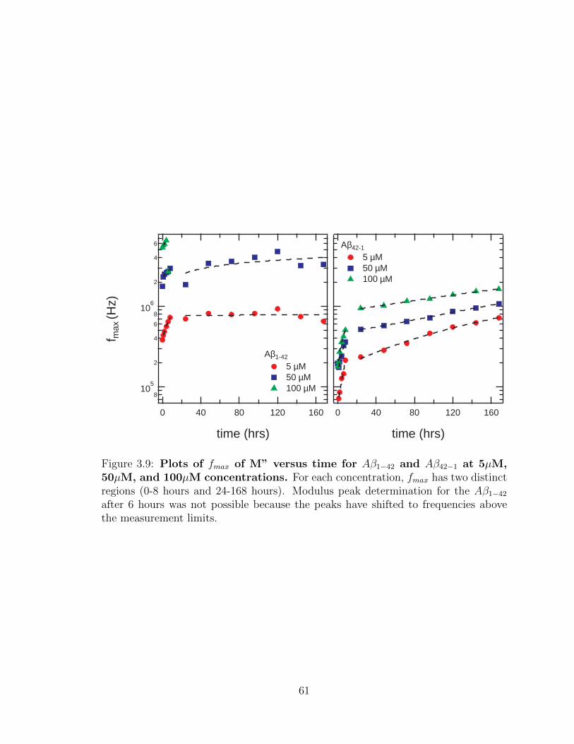
810
5
2
4
6
810
6
2
4
6
f max
(Hz)
16012080400
time (hrs)
Aβ1-42
5 µM 50 µM 100 µM
16012080400
time (hrs)
Aβ42-1
5 µM 50 µM 100 µM
Figure 3.9: Plots of fmax of M” versus time for Aβ1−42 and Aβ42−1 at 5µM,50µM, and 100µM concentrations. For each concentration, fmax has two distinctregions (0-8 hours and 24-168 hours). Modulus peak determination for the Aβ1−42after 6 hours was not possible because the peaks have shifted to frequencies abovethe measurement limits.
61
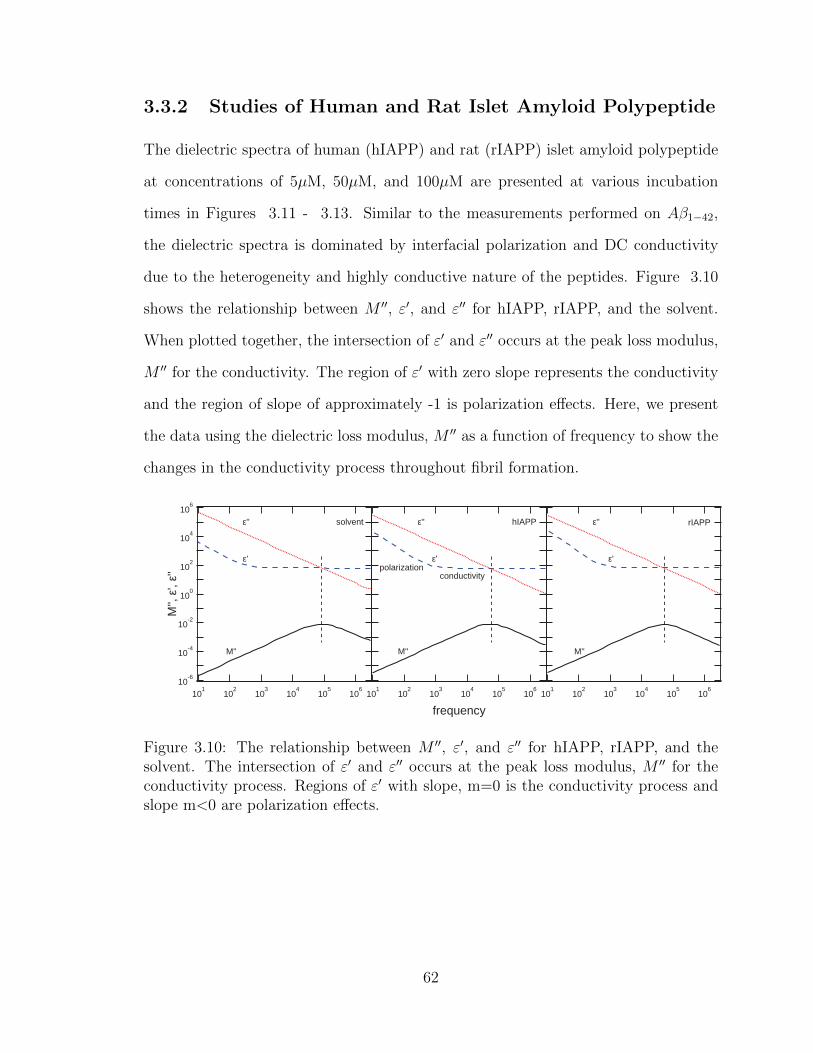
3.3.2 Studies of Human and Rat Islet Amyloid Polypeptide
The dielectric spectra of human (hIAPP) and rat (rIAPP) islet amyloid polypeptide
at concentrations of 5µM, 50µM, and 100µM are presented at various incubation
times in Figures 3.11 - 3.13. Similar to the measurements performed on Aβ1−42,
the dielectric spectra is dominated by interfacial polarization and DC conductivity
due to the heterogeneity and highly conductive nature of the peptides. Figure 3.10
shows the relationship between M ′′, ε′, and ε′′ for hIAPP, rIAPP, and the solvent.
When plotted together, the intersection of ε′ and ε′′ occurs at the peak loss modulus,
M ′′ for the conductivity. The region of ε′ with zero slope represents the conductivity
and the region of slope of approximately -1 is polarization effects. Here, we present
the data using the dielectric loss modulus, M ′′ as a function of frequency to show the
changes in the conductivity process throughout fibril formation.
10-6
10-4
10-2
100
102
104
106
M'',
ε',
ε''
101
102
103
104
105
106
solvent
101
102
103
104
105
106
frequency
hIAPP
101
102
103
104
105
106
rIAPP
M'' M'' M''
ε' ε' ε'
ε''ε''ε''
conductivitypolarization
Figure 3.10: The relationship between M ′′, ε′, and ε′′ for hIAPP, rIAPP, and thesolvent. The intersection of ε′ and ε′′ occurs at the peak loss modulus, M ′′ for theconductivity process. Regions of ε′ with slope, m=0 is the conductivity process andslope m<0 are polarization effects.
62
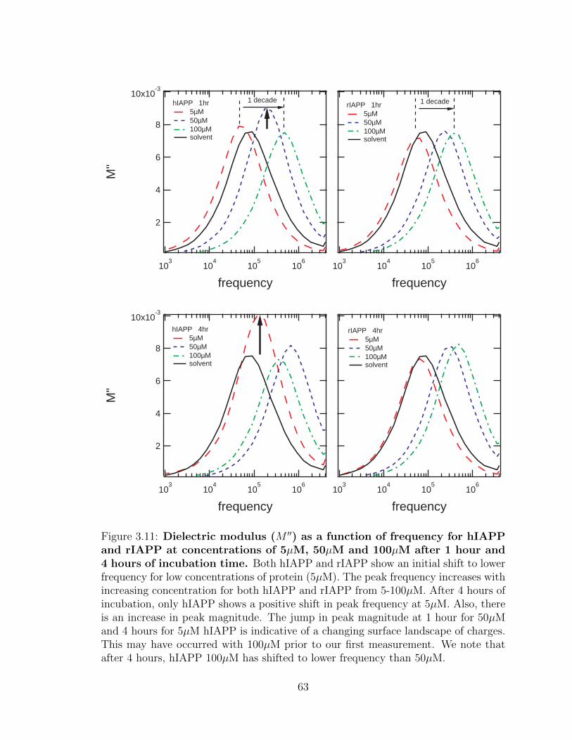
103
104
105
106
frequency
rIAPP 4hr 5µM 50µM 100µM solvent
103
104
105
106
frequency
rIAPP 1hr 5µM 50µM 100µM solvent
10x10-3
8
6
4
2
M"
103
104
105
106
frequency
hIAPP 4hr 5µM 50µM 100µM solvent
10x10-3
8
6
4
2
M"
103
104
105
106
frequency
hIAPP 1hr 5µM 50µM 100µM solvent
1 decade 1 decade
Figure 3.11: Dielectric modulus (M ′′) as a function of frequency for hIAPPand rIAPP at concentrations of 5µM, 50µM and 100µM after 1 hour and4 hours of incubation time. Both hIAPP and rIAPP show an initial shift to lowerfrequency for low concentrations of protein (5µM). The peak frequency increases withincreasing concentration for both hIAPP and rIAPP from 5-100µM. After 4 hours ofincubation, only hIAPP shows a positive shift in peak frequency at 5µM. Also, thereis an increase in peak magnitude. The jump in peak magnitude at 1 hour for 50µMand 4 hours for 5µM hIAPP is indicative of a changing surface landscape of charges.This may have occurred with 100µM prior to our first measurement. We note thatafter 4 hours, hIAPP 100µM has shifted to lower frequency than 50µM.
63

10x10-3
8
6
4
2
M"
103
104
105
106
frequency
hIAPP 6hr 5µM 50µM 100µM solvent
10x10-3
8
6
4
2
M"
103
104
105
106
frequency
hIAPP 24hr 5µM 50µM 100µM solvent
103
104
105
106
frequency
rIAPP 24hr 5µM 50µM 100µM solvent
103
104
105
106
frequency
rIAPP 6hr 5µM 50µM 100µM solvent
Figure 3.12: Dielectric modulus (M ′′) as a function of frequency for hIAPPand rIAPP at concentrations of 5µM, 50µM and 100µM after 6 hours and24 hours of incubation time. After 24 hours of incubation, the rIAPP 5µM showsa small positive shift in frequency for the first time, but is less than half that of thehIAPP. The hIAPP and rIAPP 50µM solutions display similar peak frequency shifts.The increase in magnitude of 50µM and decrease in magnitude of 100µM at 6 hoursindicates surface changes due to fibril formation. We note that the hIAPP 100µM isat lower frequency than 50µM.
64
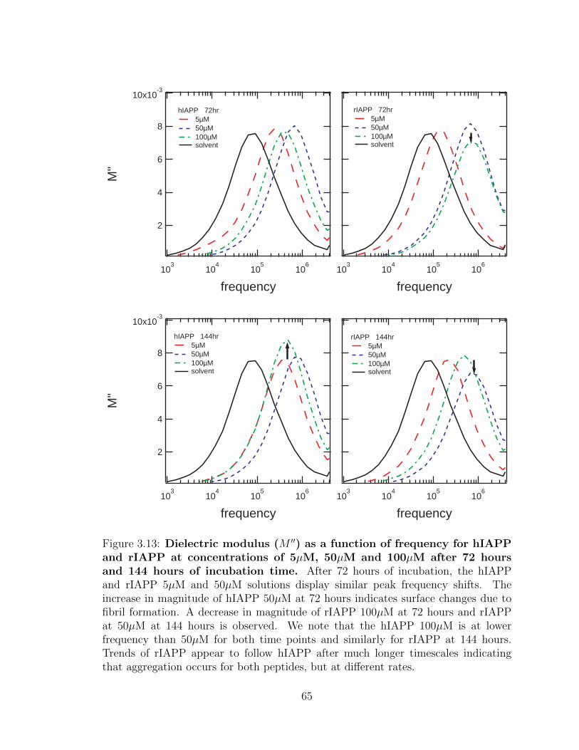
10x10-3
8
6
4
2
M"
103
104
105
106
frequency
hIAPP 72hr 5µM 50µM 100µM solvent
103
104
105
106
frequency
rIAPP 144hr 5µM 50µM 100µM solvent
103
104
105
106
frequency
rIAPP 72hr 5µM 50µM 100µM solvent
10x10-3
8
6
4
2
M"
103
104
105
106
frequency
hIAPP 144hr 5µM 50µM 100µM solvent
Figure 3.13: Dielectric modulus (M ′′) as a function of frequency for hIAPPand rIAPP at concentrations of 5µM, 50µM and 100µM after 72 hoursand 144 hours of incubation time. After 72 hours of incubation, the hIAPPand rIAPP 5µM and 50µM solutions display similar peak frequency shifts. Theincrease in magnitude of hIAPP 50µM at 72 hours indicates surface changes due tofibril formation. A decrease in magnitude of rIAPP 100µM at 72 hours and rIAPPat 50µM at 144 hours is observed. We note that the hIAPP 100µM is at lowerfrequency than 50µM for both time points and similarly for rIAPP at 144 hours.Trends of rIAPP appear to follow hIAPP after much longer timescales indicatingthat aggregation occurs for both peptides, but at different rates.
65

The time evolution of both hIAPP and rIAPP shows a shift towards higher fre-
quency with increasing concentrations of 5µM, 50µM, and 100µM at each time point.
Figures 3.14 - 3.16 show the progression of dielectric modulus shifts for 5µM, 50µM,
and 100µM hIAPP and rIAPP as compared to the solvent on two different time scales.
The 5µM hIAPP has an initial shift towards lower frequency of -0.2 decade and
then continues to shift up to +0.3 decade at 6 hours. Beyond 6 hours, there is a
continuing shift up to +0.7 decade after 144 hours. The rIAPP also has an initial
shift towards lower frequency of -0.2 decade, then continues to shift towards the same
frequency as the solvent after 6 hours. The shift continues gradually up to +0.4
decade after 144 hours.
The 50µM hIAPP has an initial shift towards high frequency of half of a decade
and continues to shift up to a decade at 6 hours. At 144 hours, there is only a small
shift. The 50µM rIAPP has a small initial shift of half of a decade, then up to +0.6
decade at 6 hours, and continues gradually up to a decade after 144 hours.
The 100µM hIAPP has an initial shift towards high frequency of +0.8 decade,
then a shift towards lower frequency at +0.6 decade after 6 hours. The peak then
continues to shift back towards higher frequency of +0.8 decade after 144 hours. The
100µM rIAPP has a similar initial shift of +0.7 decade, then continues to shift to
+0.8 decade for 6 hours and beyond.
66

103
104
105
106
frequency
rIAPP 5µM 1 hr 24 hr 72 hr 144 hr solvent
103
104
105
106
frequency
rIAPP 5µM 1 hr 4 hr 6 hr 24 hr solvent
10x10-3
8
6
4
2
M"
103
104
105
106
frequency
hIAPP 5µM 1 hr 4 hr 6 hr 24 hr solvent
10x10-3
8
6
4
2
M"
103
104
105
106
frequency
hIAPP 5µM 1 hr 24 hr 72 hr 144 hr solvent
Figure 3.14: Time evolution for 5µM rIAPP and hIAPP for 0-24 hours and1-144 hours (6 days). The hIAPP solution displays a larger frequency shift thanrIAPP in the first 24 hours and a spike in the magnitude of M ′′ at 4 hours. BothhIAPP and rIAPP display similar behavior beyond 24 hours.
67
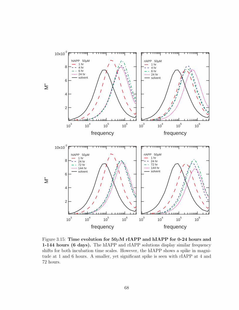
103
104
105
106
frequency
rIAPP 50µM 1 hr 4 hr 6 hr 24 hr solvent
10x10-3
8
6
4
2
M"
103
104
105
106
frequency
hIAPP 50µM 1 hr 4 hr 6 hr 24 hr solvent
10x10-3
8
6
4
2
M"
103
104
105
106
frequency
hIAPP 50µM 1 hr 24 hr 72 hr 144 hr solvent
103
104
105
106
frequency
rIAPP 50µM 1 hr 24 hr 72 hr 144 hr solvent
Figure 3.15: Time evolution for 50µM rIAPP and hIAPP for 0-24 hours and1-144 hours (6 days). The hIAPP and rIAPP solutions display similar frequencyshifts for both incubation time scales. However, the hIAPP shows a spike in magni-tude at 1 and 6 hours. A smaller, yet significant spike is seen with rIAPP at 4 and72 hours.
68

10x10-3
8
6
4
2
M"
103
104
105
106
frequency
hIAPP 100µM 1 hr 4 hr 6 hr 24 hr solvent
10x10-3
8
6
4
2
M"
103
104
105
106
frequency
hIAPP 100µM 1 hr 24 hr 72 hr 144 hr solvent
103
104
105
106
frequency
rIAPP 100µM 1 hr 24 hr 72 hr 144 hr solvent
103
104
105
106
frequency
rIAPP 100µM 1 hr 4 hr 6 hr 24 hr solvent
Figure 3.16: Time evolution for 100µM hIAPP and rIAPP for 0-24 hoursand 1-144 hours (6 days). The hIAPP frequency shift is less than that of therIAPP in the first 24 hours of incubation. The hIAPP shifts to lower frequency in thefirst 24 hours with a spike in magnitude at 24 hours. The rIAPP does not significantlychange in the first 24 hours with a spike in magnitude at 4 hours. There is little changeover time for the peak frequency for both hIAPP and rIAPP at 100µM.
69
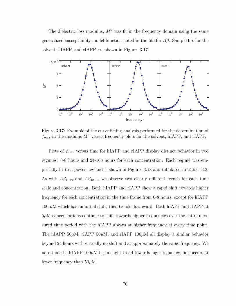
The dielectric loss modulus, M ′′ was fit in the frequency domain using the same
generalized susceptibility model function noted in the fits for Aβ. Sample fits for the
solvent, hIAPP, and rIAPP are shown in Figure 3.17.
102
103
104
105
106
102
103
104
105
106
frequency
8x10⁻³
6
4
2
0
M"
102
103
104
105
106
solvent hIAPP rIAPP
Figure 3.17: Example of the curve fitting analysis performed for the determination offmax in the modulus M” versus frequency plots for the solvent, hIAPP, and rIAPP.
Plots of fmax versus time for hIAPP and rIAPP display distinct behavior in two
regimes: 0-8 hours and 24-168 hours for each concentration. Each regime was em-
pirically fit to a power law and is shown in Figure 3.18 and tabulated in Table 3.2.
As with Aβ1−42 and Aβ42−1, we observe two clearly different trends for each time
scale and concentration. Both hIAPP and rIAPP show a rapid shift towards higher
frequency for each concentration in the time frame from 0-8 hours, except for hIAPP
100 µM which has an initial shift, then trends downward. Both hIAPP and rIAPP at
5µM concentrations continue to shift towards higher frequencies over the entire mea-
sured time period with the hIAPP always at higher frequency at every time point.
The hIAPP 50µM, rIAPP 50µM, and rIAPP 100µM all display a similar behavior
beyond 24 hours with virtually no shift and at approximately the same frequency. We
note that the hIAPP 100µM has a slight trend towards high frequency, but occurs at
lower frequency than 50µM.
70

As with Aβ, the dielectric modulus loss peaks displayed in the IAPP spectra are
dominated by interfacial polarization effects. The observation that the behavior of
rIAPP and hIAPP follow similar trends at low concentration (5µM) may be due to
a critical concentration required for beta sheet formation. At 100µM, the shift of
hIAPP to a lower frequency than that of 50µM hIAPP may be an indication that
the beta sheet formation at high concentrations has caused a shift in the interfacial
polarization signal that is not observed in rIAPP at the same concentrations.
The time evolution of the modulus loss peak in the first 24 hours is of particular
interest. A closer look at the 50µM and 100µM shows that hIAPP first shifts to
high frequency, then towards lower frequency after 24 hours. Conversely, rIAPP at
the same concentrations continues with a slight increase in frequency. The back-and-
forth shifting of the hIAPP interfacial polarization is expected due to protein surface
modulation during oligomerization and fibril formation.
5
678910
5
2
3
4
5
6789
f max
(Hz)
16012080400
time (hrs)
hIAPP 5µM 50µM 100µM
16012080400
time (hrs)
rIAPP 5µM 50µM 100µM
Figure 3.18: Plots of fmax of M” versus time for hIAPP and rIAPP at 5µM,50µM, and 100µM concentrations. Each concentration is fit to two power lawfits: one from 0-8 hours and one from 24-168.
71

hIAPP rIAPPXM C (105) A (105) k XM C (105) A (105) k
0-85µM 2.79 -23.0 -0.30 5µM 0.55 0.15 1.4350µM -25.2 278 0.02 50µM 1.77 5.22 0.52
hours 100µM 2.59 20.5 -0.41 100µM 3.87 1.16 1.36
24-1685µM 1.12 0.41 0.85 5µM 0.83 0.11 0.9750µM 6.08 0.02 1.32 50µM 6.02 0.00 3.16
hours 100µM 3.39 0.00 2.04 100µM 10.1 -438 -0.66
Table 3.2: Parameters of the power law fits to the fmax versus time for M ′′ in theform f(t) = C + Atk at concentrations XM = 5µM, 50µM, and 100µM for hIAPPand rIAPP.
72

3.4 Conclusions
Studies of these peptides at room temperature reveal that there is a large contribu-
tion to the conductivity and space-charge polarization due to the heterogeneity of the
peptide-solvent mixture. In the presence of strong space-charge polarization effects,
the dielectric modulus is often the preferred parameter for probing dielectric proper-
ties. The dielectric modulus reveals a conductivity relaxation peak that changes with
concentration and incubation time.
Both the Aβ1−42 and scrambled Aβ42−1 display a positive shift in frequency of
the conductivity relaxation peak. However, the Aβ1−42 displays an instant shift and
a much more rapid change in the first 8 hours of measurement than that of the
scrambled Aβ42−1. The shifts are larger and faster with increasing concentration
from 5µM to 100µM. The Aβ1−42 appears to reach a final state after the first day of
measurements, where the scrambled Aβ42−1 continues to gradually shift over the 7
days. This may be an indication that both the Aβ1−42 and scrambled Aβ42−1 undergo
some form of aggregation, but the process with the Aβ1−42 is faster and with a larger
frequency shift. The conformation differences in Aβ1−42 versus Aβ42−1 is observed in
the conductivity relaxation. A higher organized, tightly packed β-sheet should give
rise to more ordering in the space-charge polarization.
Measurements of the hIAPP and rIAPP also show a positive shift in frequency
for all concentrations, except the hIAPP at 100µM which shifts to lower frequency.
The trends observed in the measurements of IAPP indicates that the aggregation
behavior may be dependant on the peptide concentration. At 5µM, the hIAPP and
rIAPP follow similar trends, though a fast and larger shift is observed with hIAPP.
At 50µM, the hIAPP against shifts faster and to higher frequency, but does not
shift after 24 hours, where rIAPP continues to shift. At 100µM, hIAPP shifts to
lower frequency in the first 24 hours, then does not shift for the remaining incubation
time. The rIAPP shifts to higher frequencies and continues to shift over time. It is
73
also notable that the hIAPP 100µM shifts to lower frequency than hIAPP 50 µM,
where rIAPP is similar for 50µM and 100µM. One possibility is that 5µM is below
some critical concentration necessary for fibril formation, or it requires a much longer
incubation time, hence the continuation of the frequency shift. The 50µM follows a
similar trend observed for Aβ1−42 and scrambled Aβ42−1. The behavior of hIAPP and
rIAPP at 100µM would be interesting for further examination.
Trends in the maximum amplitude of the dielectric loss modulus, M ′′, are noted
in Figures 3.2 - 3.4 and 3.11 - 3.13. The amyloidogenic peptides Aβ1−42 and hIAPP
demonstrate spikes of increased magnitude of M ′′ at several timepoints and concentra-
tions. No spikes were observed for the non-amyloidogenic analogs. The intermittent
spikes in M ′′ are representative of a high fraction of oligomer structures in the ensem-
ble. During nucleation and oligomer formation, hydrophobic and hydrophilic regions
of amyloidogenic peptides reorganize in conformations that favor β-sheet formation
[48, 49, 50]. This results in an increase to the number of accessible mobile charge car-
riers in the solution, as reflected in an increase of the magnitude of M ′′. The charges
carriers are then restricted upon the formation of fibrils, resulting in a change in mag-
nitude of M ′′ towards that of the solvent. The non-amyloidogenic peptides do not
display these spikes because they are not expected to form intermediary oligomeric
structures and fibrils. However, they may aggregate in other conformations that
would explain the increase in frequency of M ′′, but not magnitude.
74
Chapter 4
Dielectric Studies of
Amyloidogenic Peptides in
Deionized Water Buffer at Low
Temperature
4.1 Overview
Protein association and aggregation causes a redistribution of biological water
molecules at the protein-water interface [143, 144]. Studies show that amyloidogenic
aggregates are characterized by an increased number of poorly dehydrated hydrogen
backbones and large surface densities of patches of bulk like water which favor protein
association [145, 144]. The water dynamics in the vicinity of the amyloidogenic ag-
gregates is different than the monomeric form and thus there is an increase of patches
which are occupied by molecules with bulk-like water behavior (i.e. no translations
or rotations). The change on the surface depends on how many patches of structural
defects remain after the formation of dimers, tetramers, oligomers, and protofibrils
75
[143]. We hypothesize that this change in the long-lived water structures provides
the change in the dielectric relaxation signal of the structure. Our theoretical model
suggests that measurement over a wide range of frequencies produces a differentiated
signal for the different configurations of protein-water interface.
In this chapter, dielectric spectroscopy data and analysis are presented for two
amyloidogenic peptides and their non-amyloidogenic analogs. Amyloidogenic pep-
tides Aβ1−42 and human islet amyloid polypeptide, hIAPP22−27 were used as models
for studying protein aggregation in a deionized water buffer. Deionized water was
chosen as a buffer to first study the peptides in the absence of any other biological
fluids and proteins. Their non-amyloidogenic analogs, scrambled Aβ42−1 and rat islet
amyloid polypeptide, rIAPP20−29 were selected as control materials. Measurements
were performed from room temperature down to cryogenic temperature in order to
study the relaxation kinetics. Trends of dielectric spectra as a function of incubation
time and temperature are explored within.
4.2 Sample Preparation and Data Collection
Lyophilized peptides were obtained from AnaSpec, Inc in quantities of 0.5 mg and 1.0
mg. The vials were stored at approximately -20C until the time of reconstitution.
Both the Aβ1−42 and Aβ42−1 were first rehydrated using 35µL 1% NH4OH added
to 0.5mg of protein to ensure that the solution was first driven to a monomeric
state. Deionized water, 18.2MΩ·cm minimum, was used to dilute and rehydrate the
peptides to a concentration of approximately 100µM and stored in a sterile vial. A
separate sample was prepared for each time point. The samples were then mixed by
repeated inversion of the vials and set to incubate for 0, 8, 24, 48, or 120 hours at
room temperature. Using turbidimetric measurements, Jarrett et al. showed that
Aβ1−42 in a concentration of 20µM began immediate oligomerization and reached
76
a final state at approximately 20 hours [146]. Rhodes et al. showed that hIAPP
in a concentration of 20µM began oligomerization after approximately 40 hours of
incubation and reached a final state at approximately 100 hours [147]. Glycerol,
99% minimum from Sigma was then added to a final concentration of 50µM peptide
in 50%-50% by weight DI H2O-glycerol solvent. The samples were again mixed by
repeated inversion of the vials. The samples were then placed in the Novocontrol
BDS 1307 stainless steel sample cell.
Data were collected using the Novocontrol Alpha-A Analyzer and Quatro Cryosys-
tem in gain phase measurement mode with an AC probing voltage of 1.000 VRMS. A
liquid nitrogen cryostat was used to control temperature from 283K down to 133K
at 5K intervals. We selected 60 data points in a frequency range from 2.00 × 10⁷ −
4.78 × 10⁻² Hz, spaced evenly in a logarithmic scale. Data for each temperature
point was collected in duplicate. The first of the duplicates were during temperature
stabilization and were discarded from analysis.
4.3 Results and Discussions
4.3.1 Studies of Aβ1−42 and Scrambled Aβ42−1
The dielectric spectra of Aβ1−42, scrambled Aβ42−1, and the solvent shows two relax-
ation processes (α and β) and low-frequency DC conductivity below 228K, depicted
in Figure 4.1. At temperatures above 228K, the relaxation processes are either at
frequencies above the range of the Alpha-A Analyzer or the conductivity dominates
the spectra. The fast, α-relaxation process is clearly observed at 228K at a frequency
of approximately 107 Hz in both the real and imaginary parts of the permittivity.
The slower β-relaxation process is clearly observed at approximately 104 Hz at 228K.
With decreasing temperature the peaks of the α- and β-relaxation processes shift
towards lower frequency. The α-process shifts faster than the β-process causing the
77

228K 223K 218K 213K 208K 203K
100 10
2 104 10
6
frequency
228K 223K 218K 213K 208K 203K
100 10
2 104 10
6
68
10
2
4
68
100
2
4
68
1000
ε'
2
4
68
10
2
4
68
100
2
4
68
1000
ε''
100 10
2 104 10
6
solvent Aβ1-42 Aβ42-1
β-process
β-process
α-process
α-process
DC conductivity
Figure 4.1: Temperature evolution of the real and imaginary parts of thedielectric permittivity for the solvent, Aβ1−42, and Aβ42−1 from 228K to213K. Two relaxation processes for the real (ε′) and imaginary (ε′′) parts of thepermittivity for the solvent, Aβ1−42, and scrambled Aβ42−1 are observed.
two processes to merge below 203K and eventually cross at approximately 193K as
shown in Figure 4.2. The α-process continues to shift to very low frequencies with
decreasing temperature. At around 163K the α-process shifts to frequency out of our
measured frequency range. After the crossing of the two processes, the β-relaxation
process dominates the dielectric spectra and shifts to approximately 10−1 Hz at 133K
(Figure 4.3). Below 153K, the DC conductivity has decreased in magnitude and also
shifted to frequency below the measured range.
78

198K 193K 188K 183K 178K 173K 168K
10-1 10
1 103 10
5
frequency
198K 193K 188K 183K 178K 173K 168K
4
6
810
2
4
6
8100
2
ε'
10-1 10
1 103 10
50.1
1
10
100
1000
ε''
10-1 10
1 103 10
5
solvent Aβ1-42 Aβ42-1
β-process
β-process
α-process
α-process
DC conductivity
Figure 4.2: Temperature evolution of the real and imaginary parts of thedielectric permittivity for the solvent, Aβ1−42, and Aβ42−1 from 198K to168K. The α-relaxation process rapidly shifts to lower frequency with decreasingtemperature. In the range of 198K to 188K the two processes cross where the α-relaxation is at lower frequency than the β-relaxation process at temperatures of183K and below.
79
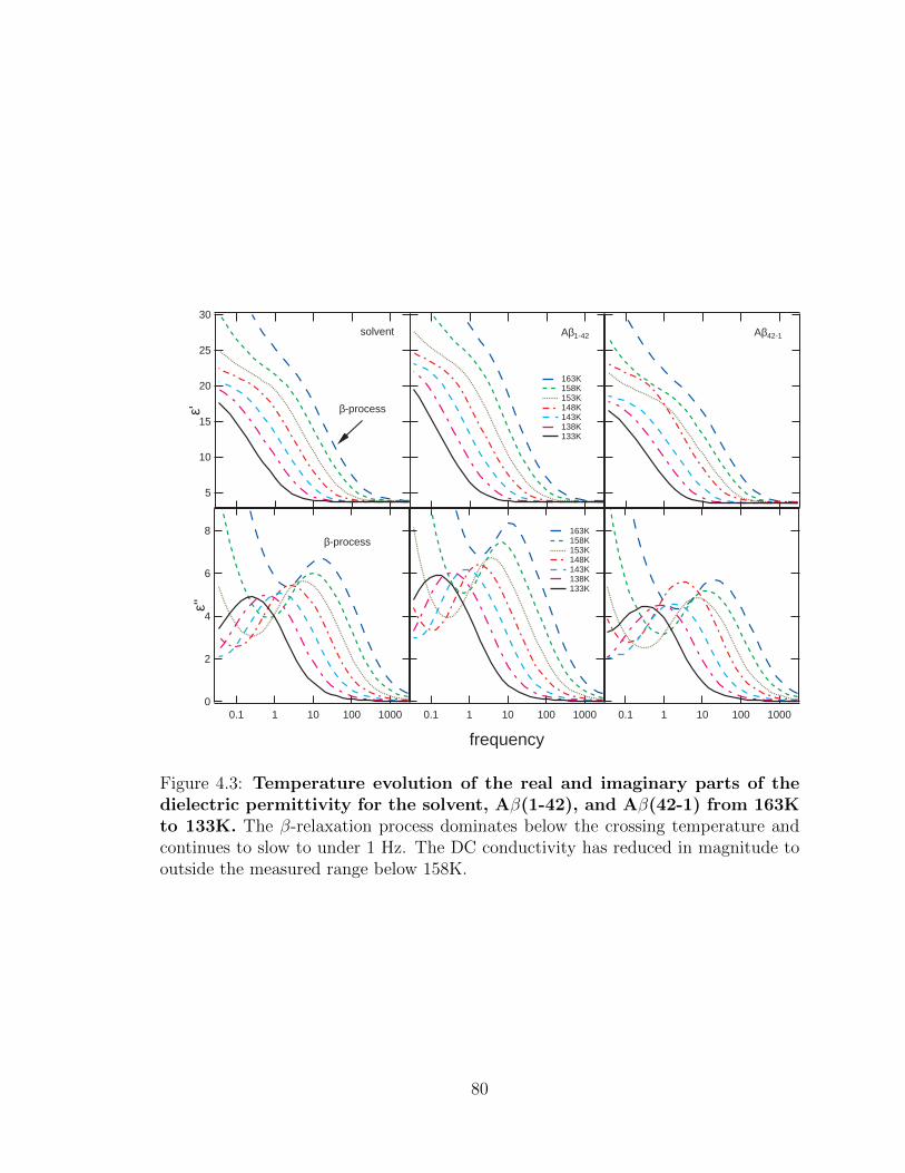
163K 158K 153K 148K 143K 138K 133K
0.1 1 10 100 1000
frequency
163K 158K 153K 148K 143K 138K 133K
30
25
20
15
10
5
ε'
0.1 1 10 100 1000
8
6
4
2
0
ε''
0.1 1 10 100 1000
solvent Aβ1-42 Aβ42-1
β-process
β-process
Figure 4.3: Temperature evolution of the real and imaginary parts of thedielectric permittivity for the solvent, Aβ(1-42), and Aβ(42-1) from 163Kto 133K. The β-relaxation process dominates below the crossing temperature andcontinues to slow to under 1 Hz. The DC conductivity has reduced in magnitude tooutside the measured range below 158K.
80
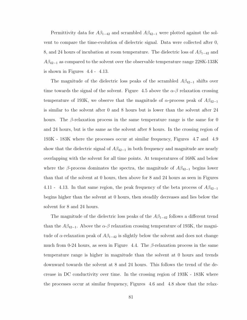
Permittivity data for Aβ1−42 and scrambled Aβ42−1 were plotted against the sol-
vent to compare the time-evolution of dielectric signal. Data were collected after 0,
8, and 24 hours of incubation at room temperature. The dielectric loss of Aβ1−42 and
Aβ42−1 as compared to the solvent over the observable temperature range 228K-133K
is shown in Figures 4.4 - 4.13.
The magnitude of the dielectric loss peaks of the scrambled Aβ42−1 shifts over
time towards the signal of the solvent. Figure 4.5 above the α-β relaxation crossing
temperature of 193K, we observe that the magnitude of α-process peak of Aβ42−1
is similar to the solvent after 0 and 8 hours but is lower than the solvent after 24
hours. The β-relaxation process in the same temperature range is the same for 0
and 24 hours, but is the same as the solvent after 8 hours. In the crossing region of
193K - 183K where the processes occur at similar frequency, Figures 4.7 and 4.9
show that the dielectric signal of Aβ42−1 in both frequency and magnitude are nearly
overlapping with the solvent for all time points. At temperatures of 168K and below
where the β-process dominates the spectra, the magnitude of Aβ42−1 begins lower
than that of the solvent at 0 hours, then above for 8 and 24 hours as seen in Figures
4.11 - 4.13. In that same region, the peak frequency of the beta process of Aβ42−1
begins higher than the solvent at 0 hours, then steadily decreases and lies below the
solvent for 8 and 24 hours.
The magnitude of the dielectric loss peaks of the Aβ1−42 follows a different trend
than the Aβ42−1. Above the α-β relaxation crossing temperature of 193K, the magni-
tude of α-relaxation peak of Aβ1−42 is slightly below the solvent and does not change
much from 0-24 hours, as seen in Figure 4.4. The β-relaxation process in the same
temperature range is higher in magnitude than the solvent at 0 hours and trends
downward towards the solvent at 8 and 24 hours. This follows the trend of the de-
crease in DC conductivity over time. In the crossing region of 193K - 183K where
the processes occur at similar frequency, Figures 4.6 and 4.8 show that the relax-
81
ation processes of Aβ1−42 nearly overlaps with the solvent and the DC conductivity
decreased in magnitude towards that of the solvent. At temperatures of 168K and
below where the β-process dominates the spectra, the magnitude of Aβ1−42 first de-
creases after 8 hours and then increases after 24 hours, but always remains larger
than the solvent as shown in Figures 4.10 - 4.12. Additionally, the peak frequency
of the beta process of Aβ1−42 starts below the solvent, then shifts above the solvent
after 8 hours, then back to lower frequency than the solvent after 24 hours.
82
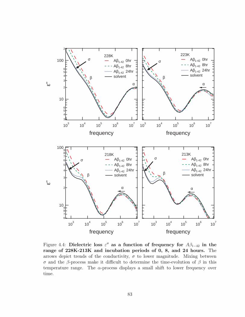
103
104
105
106
107
frequency
213K Aβ1-42 0hr Aβ1-42 8hr Aβ1-42 24hr solvent
6789
10
2
3
4
5
6789
100
ε''
103
104
105
106
107
frequency
218K Aβ1-42 0hr Aβ1-42 8hr Aβ1-42 24hr solvent
103
104
105
106
107
frequency
223K Aβ1-42 0hr Aβ1-42 8hr Aβ1-42 24hr solvent
3
456
10
2
3
456
100
2ε''
103
104
105
106
107
frequency
228K Aβ1-42 0hr Aβ1-42 8hr Aβ1-42 24hr solvent
σ σ
σσ
βα
β
α
β
α
β
α
Figure 4.4: Dielectric loss ε′′ as a function of frequency for Aβ1−42 in therange of 228K-213K and incubation periods of 0, 8, and 24 hours. Thearrows depict trends of the conductivity, σ to lower magnitude. Mixing betweenσ and the β-process make it difficult to determine the time-evolution of β in thistemperature range. The α-process displays a small shift to lower frequency overtime.
83
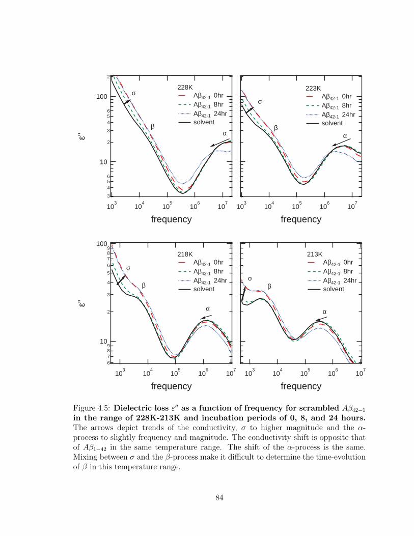
3
456
10
2
3
456
100
2ε''
103
104
105
106
107
frequency
228K Aβ42-1 0hr Aβ42-1 8hr Aβ42-1 24hr solvent
103
104
105
106
107
frequency
223K Aβ42-1 0hr Aβ42-1 8hr Aβ42-1 24hr solvent
103
104
105
106
107
frequency
213K Aβ42-1 0hr Aβ42-1 8hr Aβ42-1 24hr solvent
6789
10
2
3
4
5
6789
100
ε''
103
104
105
106
107
frequency
218K Aβ42-1 0hr Aβ42-1 8hr Aβ42-1 24hr solvent
σσ
σσ
β β
β β
α α
αα
Figure 4.5: Dielectric loss ε′′ as a function of frequency for scrambled Aβ42−1in the range of 228K-213K and incubation periods of 0, 8, and 24 hours.The arrows depict trends of the conductivity, σ to higher magnitude and the α-process to slightly frequency and magnitude. The conductivity shift is opposite thatof Aβ1−42 in the same temperature range. The shift of the α-process is the same.Mixing between σ and the β-process make it difficult to determine the time-evolutionof β in this temperature range.
84
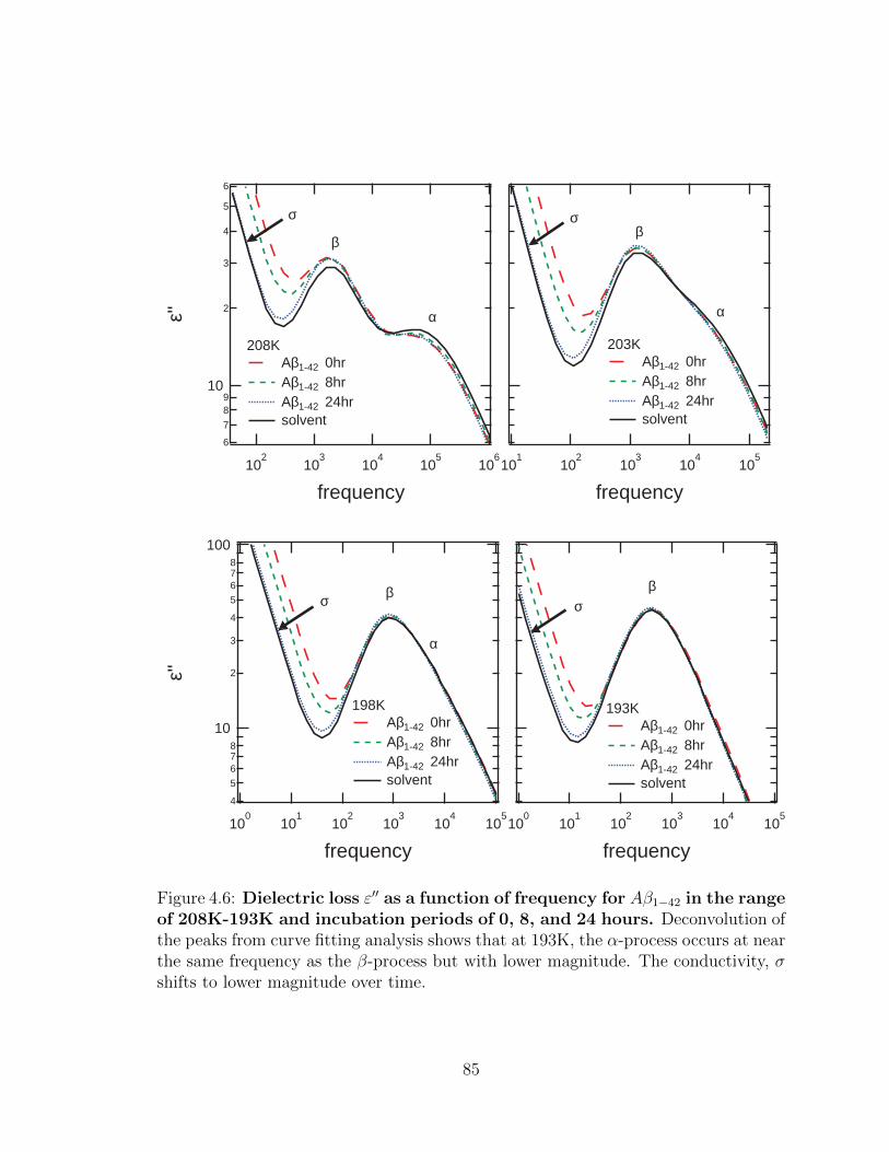
100
101
102
103
104
105
frequency
193K Aβ1-42 0hr Aβ1-42 8hr Aβ1-42 24hr solvent
101
102
103
104
105
frequency
203K Aβ1-42 0hr Aβ1-42 8hr Aβ1-42 24hr solvent
4
5
678
10
2
3
4
5
678
100
ε''
100
101
102
103
104
105
frequency
198K Aβ1-42 0hr Aβ1-42 8hr Aβ1-42 24hr solvent
6
7
89
10
2
3
4
5
6ε''
102
103
104
105
106
frequency
208K Aβ1-42 0hr Aβ1-42 8hr Aβ1-42 24hr solvent
σ
β
α
σβ
α
σ β
α
βσ
Figure 4.6: Dielectric loss ε′′ as a function of frequency for Aβ1−42 in the rangeof 208K-193K and incubation periods of 0, 8, and 24 hours. Deconvolution ofthe peaks from curve fitting analysis shows that at 193K, the α-process occurs at nearthe same frequency as the β-process but with lower magnitude. The conductivity, σshifts to lower magnitude over time.
85
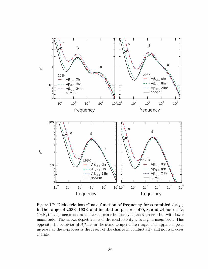
4
5
678
10
2
3
4
5
678
100
ε''
100
101
102
103
104
105
frequency
198K Aβ42-1 0hr Aβ42-1 8hr Aβ42-1 24hr solvent
100
101
102
103
104
105
frequency
193K Aβ42-1 0hr Aβ42-1 8hr Aβ42-1 24hr solvent
101
102
103
104
105
frequency
203K Aβ42-1 0hr Aβ42-1 8hr Aβ42-1 24hr solvent
6
7
89
10
2
3
4
5
6ε''
102
103
104
105
106
frequency
208K Aβ42-1 0hr Aβ42-1 8hr Aβ42-1 24hr solvent
σ σ
σσ
ββ
β β
α α
α
Figure 4.7: Dielectric loss ε′′ as a function of frequency for scrambled Aβ42−1in the range of 208K-193K and incubation periods of 0, 8, and 24 hours. At193K, the α-process occurs at near the same frequency as the β-process but with lowermagnitude. The arrows depict trends of the conductivity, σ to higher magnitude. Thisopposite the behavior of Aβ1−42 in the same temperature range. The apparent peakincrease at the β-process is the result of the change in conductivity and not a processchange.
86
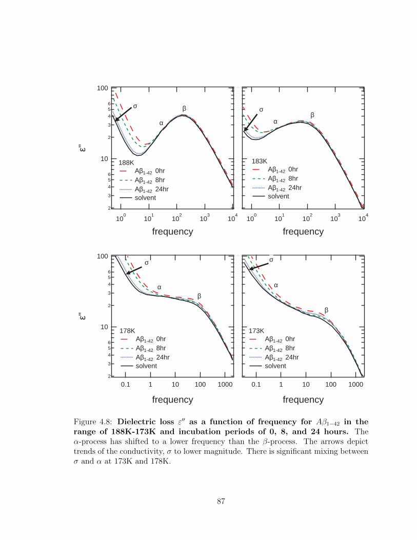
2
3
4
56
10
2
3
4
56
100
ε''
0.1 1 10 100 1000
frequency
178K Aβ1-42 0hr Aβ1-42 8hr Aβ1-42 24hr solvent
0.1 1 10 100 1000
frequency
173K Aβ1-42 0hr Aβ1-42 8hr Aβ1-42 24hr solvent
100
101
102
103
104
frequency
183K Aβ1-42 0hr Aβ1-42 8hr Aβ1-42 24hr solvent
2
3
4
56
10
2
3
4
56
100ε''
100
101
102
103
104
frequency
188K Aβ1-42 0hr Aβ1-42 8hr Aβ1-42 24hr solvent
σ σ
σ σ
ββ
β
β
α α
α α
Figure 4.8: Dielectric loss ε′′ as a function of frequency for Aβ1−42 in therange of 188K-173K and incubation periods of 0, 8, and 24 hours. Theα-process has shifted to a lower frequency than the β-process. The arrows depicttrends of the conductivity, σ to lower magnitude. There is significant mixing betweenσ and α at 173K and 178K.
87
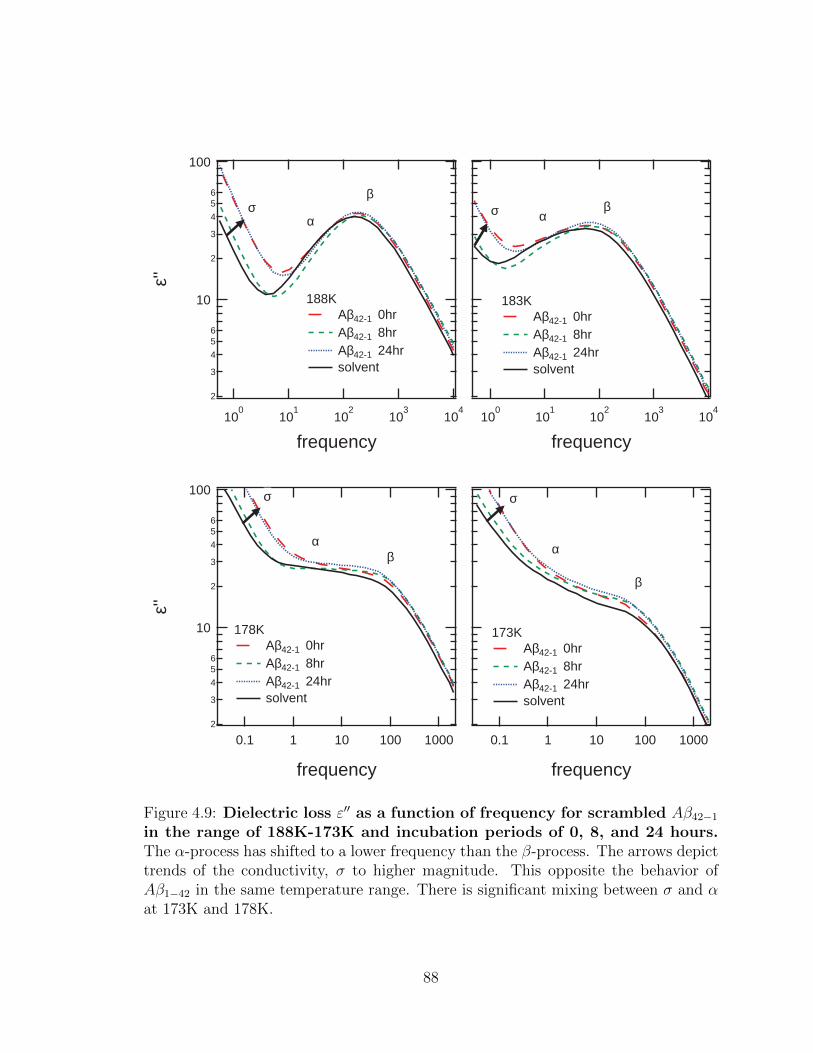
100
101
102
103
104
frequency
183K Aβ42-1 0hr Aβ42-1 8hr Aβ42-1 24hr solvent
2
3
4
56
10
2
3
4
56
100ε''
100
101
102
103
104
frequency
188K Aβ42-1 0hr Aβ42-1 8hr Aβ42-1 24hr solvent
2
3
4
56
10
2
3
4
56
100
ε''
0.1 1 10 100 1000
frequency
178K Aβ42-1 0hr Aβ42-1 8hr Aβ42-1 24hr solvent
0.1 1 10 100 1000
frequency
173K Aβ42-1 0hr Aβ42-1 8hr Aβ42-1 24hr solvent
σ σ
σ σ
ββ
β
β
α α
α α
Figure 4.9: Dielectric loss ε′′ as a function of frequency for scrambled Aβ42−1in the range of 188K-173K and incubation periods of 0, 8, and 24 hours.The α-process has shifted to a lower frequency than the β-process. The arrows depicttrends of the conductivity, σ to higher magnitude. This opposite the behavior ofAβ1−42 in the same temperature range. There is significant mixing between σ and αat 173K and 178K.
88
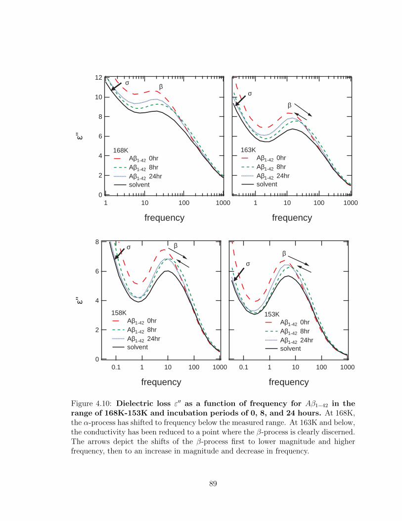
0.1 1 10 100 1000
frequency
153K Aβ1-42 0hr Aβ1-42 8hr Aβ1-42 24hr solvent
8
6
4
2
0
ε''
0.1 1 10 100 1000
frequency
158K Aβ1-42 0hr Aβ1-42 8hr Aβ1-42 24hr solvent
1 10 100 1000
frequency
163K Aβ1-42 0hr Aβ1-42 8hr Aβ1-42 24hr solvent
12
10
8
6
4
2
0
ε''
1 10 100 1000
frequency
168K Aβ1-42 0hr Aβ1-42 8hr Aβ1-42 24hr solvent
σ
σ
σ
σ
β
β
ββ
Figure 4.10: Dielectric loss ε′′ as a function of frequency for Aβ1−42 in therange of 168K-153K and incubation periods of 0, 8, and 24 hours. At 168K,the α-process has shifted to frequency below the measured range. At 163K and below,the conductivity has been reduced to a point where the β-process is clearly discerned.The arrows depict the shifts of the β-process first to lower magnitude and higherfrequency, then to an increase in magnitude and decrease in frequency.
89
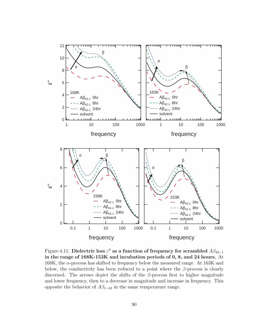
12
10
8
6
4
2
0
ε''
1 10 100 1000
frequency
168K Aβ42-1 0hr Aβ42-1 8hr Aβ42-1 24hr solvent
1 10 100 1000
frequency
163K Aβ42-1 0hr Aβ42-1 8hr Aβ42-1 24hr solvent
8
6
4
2
0
ε''
0.1 1 10 100 1000
frequency
158K Aβ42-1 0hr Aβ42-1 8hr Aβ42-1 24hr solvent
0.1 1 10 100 1000
frequency
153K Aβ42-1 0hr Aβ42-1 8hr Aβ42-1 24hr solvent
σσ
σ
σ
β
β
ββ
Figure 4.11: Dielectric loss ε′′ as a function of frequency for scrambled Aβ42−1in the range of 168K-153K and incubation periods of 0, 8, and 24 hours. At168K, the α-process has shifted to frequency below the measured range. At 163K andbelow, the conductivity has been reduced to a point where the β-process is clearlydiscerned. The arrows depict the shifts of the β-process first to higher magnitudeand lower frequency, then to a decrease in magnitude and increase in frequency. Thisopposite the behavior of Aβ1−42 in the same temperature range.
90
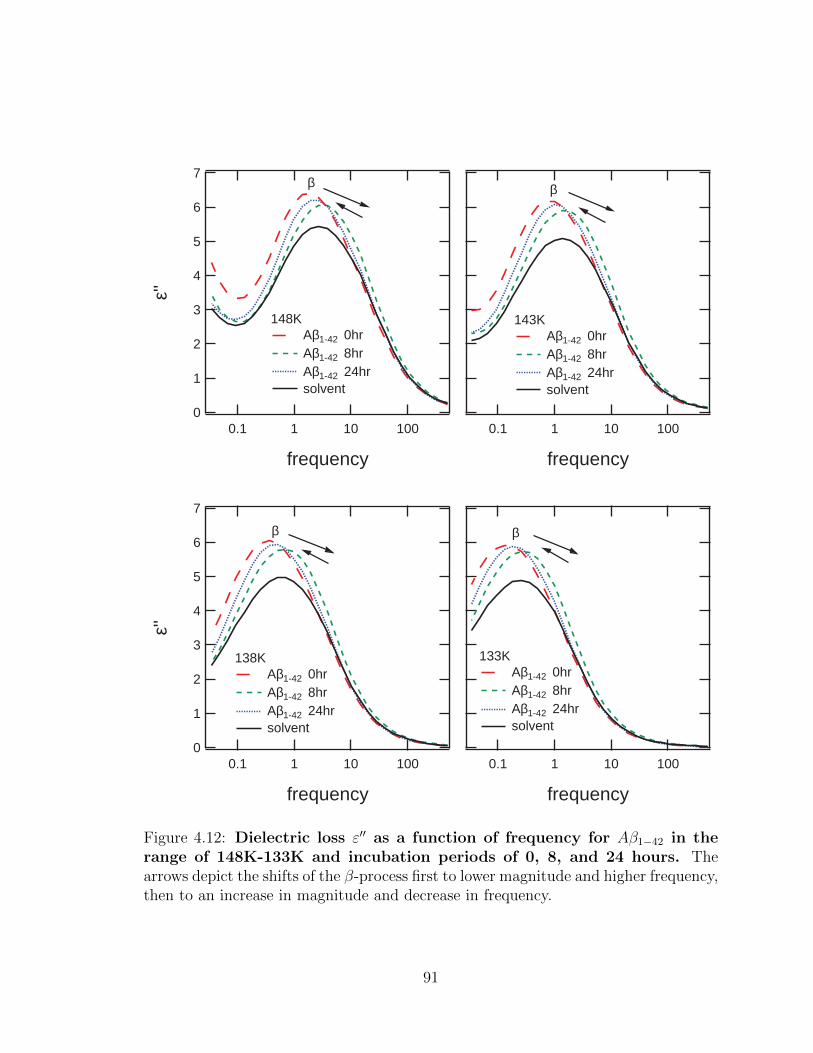
0.1 1 10 100
frequency
133K Aβ1-42 0hr Aβ1-42 8hr Aβ1-42 24hr solvent
7
6
5
4
3
2
1
0
ε''
0.1 1 10 100
frequency
138K Aβ1-42 0hr Aβ1-42 8hr Aβ1-42 24hr solvent
0.1 1 10 100
frequency
143K Aβ1-42 0hr Aβ1-42 8hr Aβ1-42 24hr solvent
7
6
5
4
3
2
1
0
ε''
0.1 1 10 100
frequency
148K Aβ1-42 0hr Aβ1-42 8hr Aβ1-42 24hr solvent
β β
β β
Figure 4.12: Dielectric loss ε′′ as a function of frequency for Aβ1−42 in therange of 148K-133K and incubation periods of 0, 8, and 24 hours. Thearrows depict the shifts of the β-process first to lower magnitude and higher frequency,then to an increase in magnitude and decrease in frequency.
91
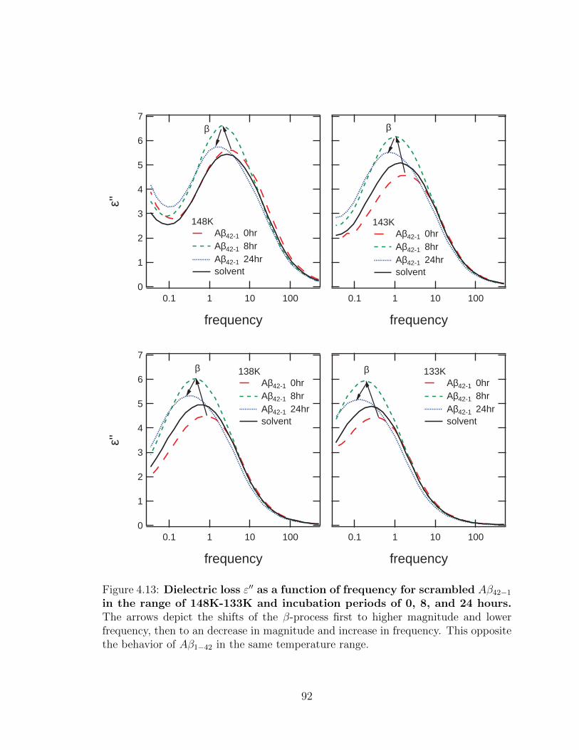
7
6
5
4
3
2
1
0
ε''
0.1 1 10 100
frequency
138K Aβ42-1 0hr Aβ42-1 8hr Aβ42-1 24hr solvent
0.1 1 10 100
frequency
133K Aβ42-1 0hr Aβ42-1 8hr Aβ42-1 24hr solvent
0.1 1 10 100
frequency
143K Aβ42-1 0hr Aβ42-1 8hr Aβ42-1 24hr solvent
7
6
5
4
3
2
1
0
ε''
0.1 1 10 100
frequency
148K Aβ42-1 0hr Aβ42-1 8hr Aβ42-1 24hr solvent
β β
β β
Figure 4.13: Dielectric loss ε′′ as a function of frequency for scrambled Aβ42−1in the range of 148K-133K and incubation periods of 0, 8, and 24 hours.The arrows depict the shifts of the β-process first to higher magnitude and lowerfrequency, then to an decrease in magnitude and increase in frequency. This oppositethe behavior of Aβ1−42 in the same temperature range.
92
Dielectric permittivity data for Aβ1−42, and Aβ42−1, and the solvent were modeled
using the WinFIT program for each temperature from 223K to 133K and at incu-
bation time points 0, 8, and 24 hours. The model functions include a power law for
conductivity and the Havriliak-Negami function for each relaxation process given by
ε∗(ω) = −i(σ0ε0ω
)N+
2∑k=1
[ε∞,k +
∆εk(1 + (iωτk)βk)γk
](4.1)
The β-relaxation process demonstrates symmetric broadening but no asymmetric
broadening over the measured temperature range. This reduces the Havriliak-Negami
function to a Cole-Davidson with γ = 1 and β < 1. The symmetric broadening pa-
rameter, β remains relatively constant over the entire temperature range at approxi-
mately 0.8. The α-relaxation process demonstrates both symmetric and asymmetric
broadening over the observed temperature range. Both β and γ spreading parameters
change with temperature. Data were fit using a least-squares minimization and the
root-mean-squared-deviation (RMSD) is reported for goodness of fit.
The α-relaxation process is observed from 228K to 168K, though in the crossing
temperatures of 198K to 183K, it overlaps with the β-process. During this tempera-
ture range, the β-relaxation process dominates. The β-relaxation process is observed
between approximately 228K down to the lowest temperature, 133K. At tempera-
tures above 208K, the DC conductivity dominates the spectra in the region of the
β-relaxation. Examples of curve fitting performed at representative temperatures are
shown in Figures 4.14 - 4.17.
Figure 4.17 shows a clear β-relaxation process with a high-frequency excess wing.
The excess wing is known to exist in certain glass-forming liquids such as glycerol [63].
The wing may exist at all temperatures but is most pronounced at low temperatures,
particularly below the glass transition. Despite efforts to characterize the excess
wing, there is no common explanation to its physical origin and thus it is treated
93
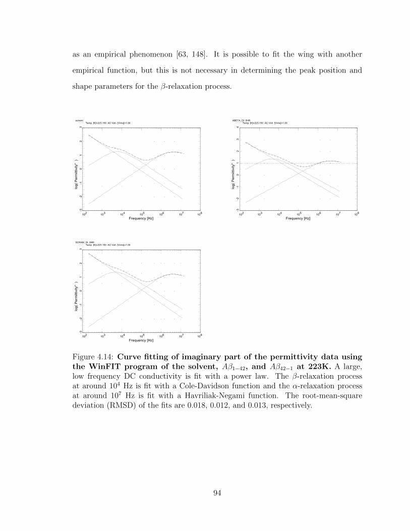
as an empirical phenomenon [63, 148]. It is possible to fit the wing with another
empirical function, but this is not necessary in determining the peak position and
shape parameters for the β-relaxation process.
102
103
104
105
106
107
108
Frequency [Hz]
-3-2
-10
12
3
log( Perm
ittivity'' )
solvent Temp. [K]=223.150 AC Volt [Vrms]=1.00
102
103
104
105
106
107
108
Frequency [Hz]
-3-2
-10
12
34
log( Perm
ittivity'' )
ABETA_DI_0HR Temp. [K]=223.150 AC Volt [Vrms]=1.00
102
103
104
105
106
107
108
Frequency [Hz]
-3-2
-10
12
3
log( Perm
ittivity'' )
SCRAM_DI_0HR Temp. [K]=223.150 AC Volt [Vrms]=1.00
Figure 4.14: Curve fitting of imaginary part of the permittivity data usingthe WinFIT program of the solvent, Aβ1−42, and Aβ42−1 at 223K. A large,low frequency DC conductivity is fit with a power law. The β-relaxation processat around 104 Hz is fit with a Cole-Davidson function and the α-relaxation processat around 107 Hz is fit with a Havriliak-Negami function. The root-mean-squaredeviation (RMSD) of the fits are 0.018, 0.012, and 0.013, respectively.
94

100
101
102
103
104
105
106
107
Frequency [Hz]
-3-2
-10
12
34
log
( P
erm
itti
vit
y''
)
solvent Temp. [K]=208.150 AC Volt [Vrms]=1.00
100
101
102
103
104
105
106
107
Frequency [Hz]
-3-2
-10
12
34
log
( P
erm
itti
vit
y''
)
ABETA_DI_0HR Temp. [K]=208.150 AC Volt [Vrms]=1.00
100
101
102
103
104
105
106
107
Frequency [Hz]
-3-2
-10
12
34
log
( P
erm
itti
vit
y''
)
SCRAM_DI_0HR Temp. [K]=208.150 AC Volt [Vrms]=1.00
Figure 4.15: Curve fitting of imaginary part of the permittivity data usingthe WinFIT program of the solvent, Aβ1−42, and Aβ42−1 at 208K. A large,low frequency DC conductivity is fit with a power law. The β-relaxation process ataround 103 Hz is fit with a Cole-Davidson function and the α-relaxation process ataround 105 Hz is fit with a Havriliak-Negami function. The RMSD of the fits are0.045, 0.009, and 0.013, respectively.
95

10-1
100
101
102
103
104
105
106
Frequency [Hz]
-4-3
-2-1
01
23
log( Perm
ittivity'' )
solvent Temp. [K]=188.150 AC Volt [Vrms]=1.00
10-1
100
101
102
103
104
105
Frequency [Hz]
-3-2
-10
12
3
log( Permittivity'' )
ABETA_DI_0HR Temp. [K]=188.150 AC Volt [Vrms]=1.00
10-1
100
101
102
103
104
105
Frequency [Hz]
-3-2
-10
12
3
log( Permittivity'' )
SCRAM_DI_0HR Temp. [K]=188.150 AC Volt [Vrms]=1.00
Figure 4.16: Curve fitting of imaginary part of the permittivity data usingthe WinFIT program of the solvent, Aβ1−42, and Aβ42−1 at 188K. A large,low frequency DC conductivity is fit with a power law. The β-relaxation processat around 103 Hz is fit with a Cole-Davidson function and the α-relaxation processat around 101 Hz is fit with a Havriliak-Negami function. Here, the α process hascrossed over to slower than β relaxation times. The RMSD of the fits are 0.008, 0.011,and 0.013, respectively.
96

10-2
10-1
100
101
102
103
104
Frequency [Hz]
01
23
45
6
Perm
ittivity''
solvent Temp. [K]=133.150 AC Volt [Vrms]=1.00
10-2
10-1
100
101
102
103
104
Frequency [Hz]0
24
68
Perm
ittivity''
ABETA_DI_0HR Temp. [K]=133.150 AC Volt [Vrms]=1.00
10-2
10-1
100
101
102
103
104
Frequency [Hz]
01
23
45
Perm
ittivity''
SCRAM_DI_0HR Temp. [K]=133.150 AC Volt [Vrms]=1.00
Figure 4.17: Curve fitting of the imaginary part of the permittivity datausing the WinFIT program of the solvent, Aβ1−42, and Aβ42−1 at 133K. Asmall, very low frequency DC conductivity is fit with a power law. The β-relaxationprocess at around 1 Hz is fit with a Cole-Davidson function and the α-relaxationprocess is not observed. The RMSD of the fits are 0.092, 0.123, and 0.082, respectively.
97
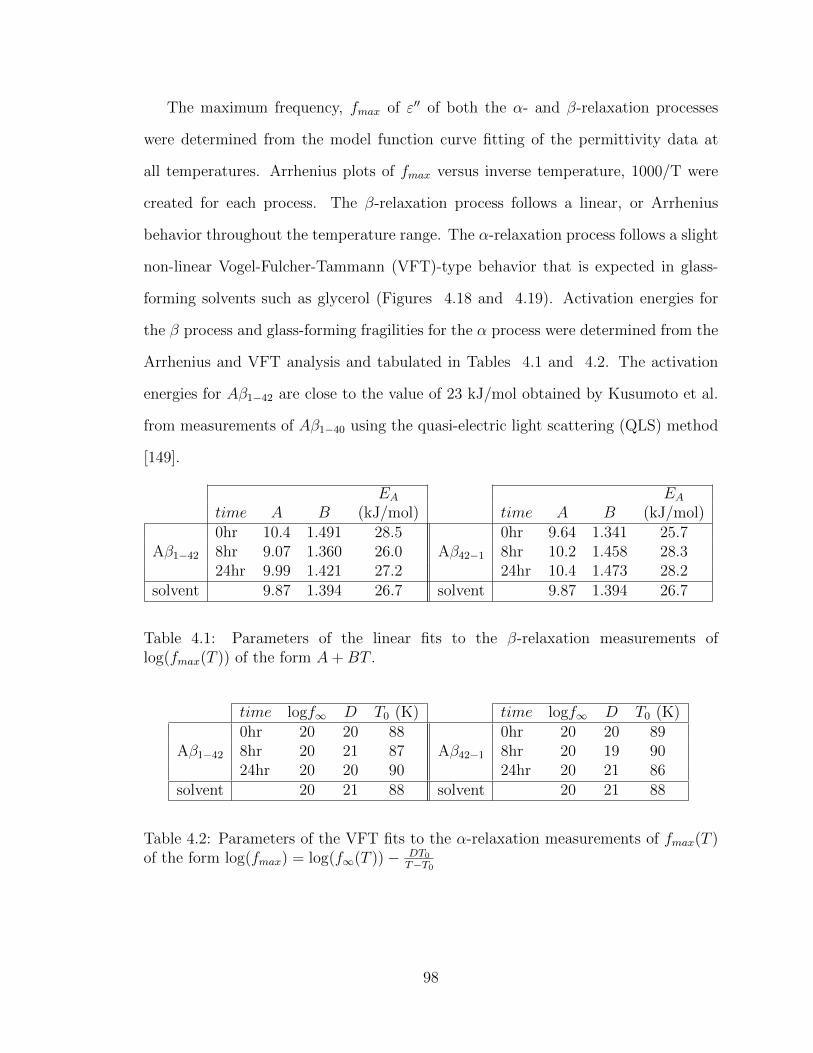
The maximum frequency, fmax of ε′′ of both the α- and β-relaxation processes
were determined from the model function curve fitting of the permittivity data at
all temperatures. Arrhenius plots of fmax versus inverse temperature, 1000/T were
created for each process. The β-relaxation process follows a linear, or Arrhenius
behavior throughout the temperature range. The α-relaxation process follows a slight
non-linear Vogel-Fulcher-Tammann (VFT)-type behavior that is expected in glass-
forming solvents such as glycerol (Figures 4.18 and 4.19). Activation energies for
the β process and glass-forming fragilities for the α process were determined from the
Arrhenius and VFT analysis and tabulated in Tables 4.1 and 4.2. The activation
energies for Aβ1−42 are close to the value of 23 kJ/mol obtained by Kusumoto et al.
from measurements of Aβ1−40 using the quasi-electric light scattering (QLS) method
[149].
EA EAtime A B (kJ/mol) time A B (kJ/mol)
Aβ1−42
0hr 10.4 1.491 28.5Aβ42−1
0hr 9.64 1.341 25.78hr 9.07 1.360 26.0 8hr 10.2 1.458 28.324hr 9.99 1.421 27.2 24hr 10.4 1.473 28.2
solvent 9.87 1.394 26.7 solvent 9.87 1.394 26.7
Table 4.1: Parameters of the linear fits to the β-relaxation measurements oflog(fmax(T )) of the form A+BT .
time logf∞ D T0 (K) time logf∞ D T0 (K)
Aβ1−42
0hr 20 20 88Aβ42−1
0hr 20 20 898hr 20 21 87 8hr 20 19 9024hr 20 20 90 24hr 20 21 86
solvent 20 21 88 solvent 20 21 88
Table 4.2: Parameters of the VFT fits to the α-relaxation measurements of fmax(T )of the form log(fmax) = log(f∞(T ))− DT0
T−T0
98

8
6
4
2
0
log(
f max
)
7.57.06.56.05.55.04.5
1000/T
solvent
7.57.06.56.05.55.04.5
1000/T
Aβ1-42 0hr
7.57.06.56.05.55.04.5
1000/T
Aβ1-42 24hr8
6
4
2
0
log(
f max
)
7.57.06.56.05.55.04.5
1000/T
Aβ1-42 8hr
Figure 4.18: Arrhenius plots of fmax versus inverse temperature for Aβ1−42over time. The α-relaxation process follows a VFT behavior whereas the β-relaxation process follows an Arrhenius, or linear behavior. The α-process departsfrom the VFT curvature at low temperature.
99

8
6
4
2
0
log(
f max
)
7.57.06.56.05.55.04.5
1000/T
solvent
7.57.06.56.05.55.04.5
1000/T
Aβ42-1 24hr
8
6
4
2
0
log(
f max
)
7.57.06.56.05.55.04.5
1000/T
Aβ42-1 8hr
7.57.06.56.05.55.04.5
1000/T
Aβ42-1 0hr
Figure 4.19: Arrhenius plots of fmax versus inverse temperature for scram-bled Aβ42−1 over time. The α-relaxation process follows a VFT behavior whereasthe β-relaxation process follows an Arrhenius, or linear behavior. The α-processdeparts from the VFT curvature at low temperature.
100
Onsager described the enhancement of permanent dipoles by polarization of the
environment, or reaction field [150]. Here, the dielectric strength (∆ε) is related to
the dipole moment (µ) by:
∆ε =1
3ε0F
µ2
kBT
N
V(4.2)
where N/V is the volume density of dipoles and F is a correction for the reaction
field. Kirkwood and Frohlich further extended the theory for interacting dipoles by
introducing a factor, g with g<1 for anti-parallel dipoles and g>1 for parallel dipoles:
∆ε =1
3ε0Fg
µ2
kBT
N
V(4.3)
From this equation, it is evident that the dielectric strength is proportional to the
dipole moment squared.
The macroscopic resulting dipole moment of a protein solution can present struc-
tural information about the aggregates. The α-helix and random coils will give a
significant contribution to the dipole moment [151, 130]. If β-sheets form, the dipole
moment should decrease for anti-parallel conformations and remain relatively strong
for parallel arrangements. Figure 4.20 shows that over time, Aβ1−42 first has an in-
crease, then decreases in the dielectric strength as fibril formation progresses, whereas
the non-amyloidogenic Aβ42−1 does not change over time. Studies using FTIR have
indicated that the structure of the Aβ1−42 displays an anti-parallel β-sheet [152, 153].
This is in agreement with our results showing a decrease in the dielectric strength,
and thus, the dipole moment as fibrils form. The initial increase in dipole moment
could be an indication of a high concentration of oligomers, which are known to form
circular micelles [154]. A circular form round present an alignment of dipoles that
would have additive dipole moments.
101
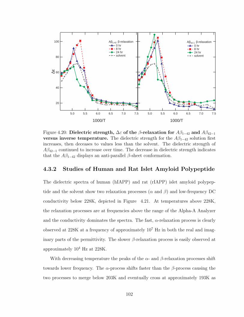
7.57.06.56.05.55.0
1000/T
Aβ42-1 β-relaxation 0 hr 8 hr 24 hr solvent
100
80
60
40
20
∆ε
7.57.06.56.05.55.0
1000/T
Aβ1-42 β-relaxation 0 hr 8 hr 24 hr solvent
Figure 4.20: Dielectric strength, ∆ε of the β-relaxation for Aβ1−42 and Aβ42−1versus inverse temperature. The dielectric strength for the Aβ1−42 solution firstincreases, then deceases to values less than the solvent. The dielectric strength ofAβ42−1 continued to increase over time. The decrease in dielectric strength indicatesthat the Aβ1−42 displays an anti-parallel β-sheet conformation.
4.3.2 Studies of Human and Rat Islet Amyloid Polypeptide
The dielectric spectra of human (hIAPP) and rat (rIAPP) islet amyloid polypep-
tide and the solvent show two relaxation processes (α and β) and low-frequency DC
conductivity below 228K, depicted in Figure 4.21. At temperatures above 228K,
the relaxation processes are at frequencies above the range of the Alpha-A Analyzer
and the conductivity dominates the spectra. The fast, α-relaxation process is clearly
observed at 228K at a frequency of approximately 107 Hz in both the real and imag-
inary parts of the permittivity. The slower β-relaxation process is easily observed at
approximately 104 Hz at 228K.
With decreasing temperature the peaks of the α- and β-relaxation processes shift
towards lower frequency. The α-process shifts faster than the β-process causing the
two processes to merge below 203K and eventually cross at approximately 193K as
102
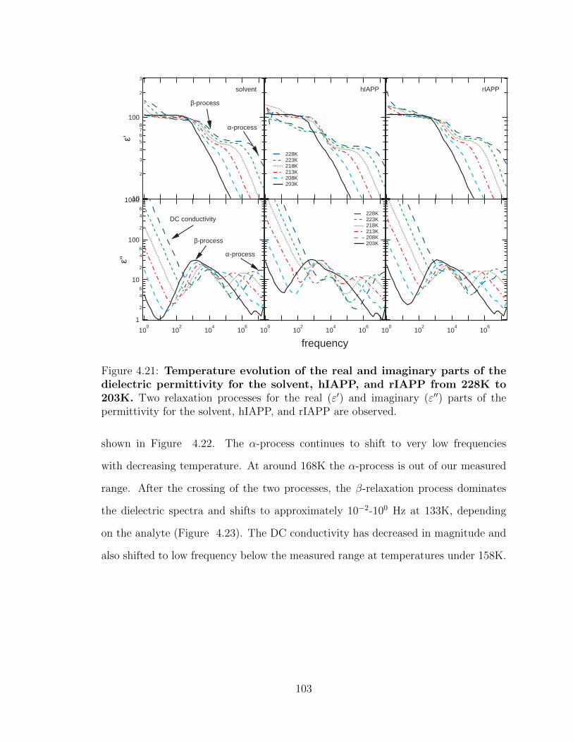
228K 223K 218K 213K 208K 203K
100 10
2 104 10
6
frequency
228K 223K 218K 213K 208K 203K
10
2
3
4
5678
100
2
3
ε'
100 10
2 104 10
6 1
2
4
6
10
2
4
6
100
2
4
6
1000
ε''
100 10
2 104 10
6
solvent hIAPP rIAPP
DC conductivity
α-process
α-process
β-process
β-process
Figure 4.21: Temperature evolution of the real and imaginary parts of thedielectric permittivity for the solvent, hIAPP, and rIAPP from 228K to203K. Two relaxation processes for the real (ε′) and imaginary (ε′′) parts of thepermittivity for the solvent, hIAPP, and rIAPP are observed.
shown in Figure 4.22. The α-process continues to shift to very low frequencies
with decreasing temperature. At around 168K the α-process is out of our measured
range. After the crossing of the two processes, the β-relaxation process dominates
the dielectric spectra and shifts to approximately 10−2-100 Hz at 133K, depending
on the analyte (Figure 4.23). The DC conductivity has decreased in magnitude and
also shifted to low frequency below the measured range at temperatures under 158K.
103

10-1 10
1 103 10
5
frequency
198K 183K 168K 193K 178K 188K 173K
198K 193K 188K 183K 178K 173K 168K
3
456
10
2
3
456
100
2
ε'
10-1 10
1 103 10
50.1
2
4
6
1
2
4
6
10
2
4
6
100
ε''
10-1 10
1 103 10
5
solvent hIAPP rIAPP
β-process
α-process
β-processα-process
Figure 4.22: Temperature evolution of the real and imaginary parts of thedielectric permittivity for the solvent, hIAPP, and rIAPP from 198K to168K. The α-relaxation process rapidly shifts to lower frequency with decreasingtemperature. In the range of 198K to 188K the two processes cross to where theα-relaxation is at lower frequency than the β-relaxation process at temperatures of183K and below.
104
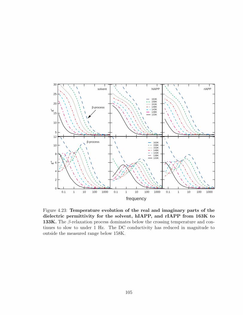
0.1 1 10 100 1000
frequency
163K 158K 153K 148K 143K 138K 133K
163K 158K 153K 148K 143K 138K 133K
30
25
20
15
10
5
ε'
0.1 1 10 100 1000
12
10
8
6
4
2
0
ε''
0.1 1 10 100 1000
β-process
β-process
solvent hIAPP rIAPP
Figure 4.23: Temperature evolution of the real and imaginary parts of thedielectric permittivity for the solvent, hIAPP, and rIAPP from 163K to133K. The β-relaxation process dominates below the crossing temperature and con-tinues to slow to under 1 Hz. The DC conductivity has reduced in magnitude tooutside the measured range below 158K.
105
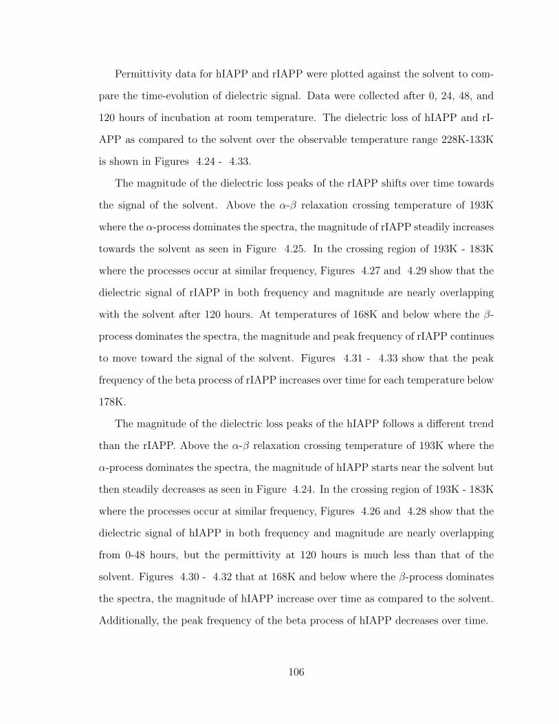
Permittivity data for hIAPP and rIAPP were plotted against the solvent to com-
pare the time-evolution of dielectric signal. Data were collected after 0, 24, 48, and
120 hours of incubation at room temperature. The dielectric loss of hIAPP and rI-
APP as compared to the solvent over the observable temperature range 228K-133K
is shown in Figures 4.24 - 4.33.
The magnitude of the dielectric loss peaks of the rIAPP shifts over time towards
the signal of the solvent. Above the α-β relaxation crossing temperature of 193K
where the α-process dominates the spectra, the magnitude of rIAPP steadily increases
towards the solvent as seen in Figure 4.25. In the crossing region of 193K - 183K
where the processes occur at similar frequency, Figures 4.27 and 4.29 show that the
dielectric signal of rIAPP in both frequency and magnitude are nearly overlapping
with the solvent after 120 hours. At temperatures of 168K and below where the β-
process dominates the spectra, the magnitude and peak frequency of rIAPP continues
to move toward the signal of the solvent. Figures 4.31 - 4.33 show that the peak
frequency of the beta process of rIAPP increases over time for each temperature below
178K.
The magnitude of the dielectric loss peaks of the hIAPP follows a different trend
than the rIAPP. Above the α-β relaxation crossing temperature of 193K where the
α-process dominates the spectra, the magnitude of hIAPP starts near the solvent but
then steadily decreases as seen in Figure 4.24. In the crossing region of 193K - 183K
where the processes occur at similar frequency, Figures 4.26 and 4.28 show that the
dielectric signal of hIAPP in both frequency and magnitude are nearly overlapping
from 0-48 hours, but the permittivity at 120 hours is much less than that of the
solvent. Figures 4.30 - 4.32 that at 168K and below where the β-process dominates
the spectra, the magnitude of hIAPP increase over time as compared to the solvent.
Additionally, the peak frequency of the beta process of hIAPP decreases over time.
106
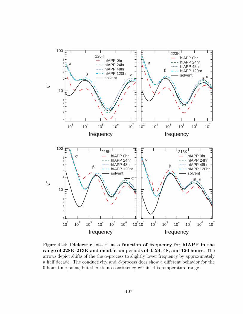
101
102
103
104
105
106
107
frequency
213K hIAPP 0hr hIAPP 24hr hIAPP 48hr hIAPP 120hr solvent
2
3
4
56
10
2
3
4
56
100
ε''
101
102
103
104
105
106
107
frequency
218K hIAPP 0hr hIAPP 24hr hIAPP 48hr hIAPP 120hr solvent
102
103
104
105
106
107
frequency
223K hIAPP 0hr hIAPP 24hr hIAPP 48hr hIAPP 120hr solvent
2
3
456
10
2
3
456
100ε''
103
104
105
106
107
frequency
228K hIAPP 0hr hIAPP 24hr hIAPP 48hr hIAPP 120hr solvent
σ σ
σσ
α α
ααββ
β β
Figure 4.24: Dielectric loss ε′′ as a function of frequency for hIAPP in therange of 228K-213K and incubation periods of 0, 24, 48, and 120 hours. Thearrows depict shifts of the the α-process to slightly lower frequency by approximatelya half decade. The conductivity and β-process does show a different behavior for the0 hour time point, but there is no consistency within this temperature range.
107

101
102
103
104
105
106
107
frequency
213K rIAPP 0hr rIAPP 24hr rIAPP 48hr rIAPP 120hr solvent
103
104
105
106
107
frequency
223K rIAPP 0hr rIAPP 24hr rIAPP 48hr rIAPP 120hr solvent
2
3
456
10
2
3
456
100ε''
103
104
105
106
107
frequency
228K rIAPP 0hr rIAPP 24hr rIAPP 48hr rIAPP 120hr solvent
2
3
4
56
10
2
3
4
56
100
ε''
101
102
103
104
105
106
107
frequency
218K rIAPP 0hr rIAPP 24hr rIAPP 48hr rIAPP 120hr solvent
σ
σ
σ σ
β β
β β
αα
αα
Figure 4.25: Dielectric loss ε′′ as a function of frequency for rIAPP in therange of 228K-213K and incubation periods of 0, 24, 48, and 120 hours. Thearrows show the trend of increasing conductivity over time. This was not observedwith hIAPP. The apparent peak increase at the β-process is most likely the result ofthe change in conductivity and not a process change. There are changes observed inthe α-process at 228K and 223K, but without a trend.
108

10-1 10
1 103 10
5
frequency
193K hIAPP 0hr hIAPP 24hr hIAPP 48hr hIAPP 120hr solvent
6
81
2
4
6
810
2
4
6
ε''
10-1 10
1 103 10
5
frequency
198K hIAPP 0hr hIAPP 24hr hIAPP 48hr hIAPP 120hr solvent
100
101
102
103
104
105
106
frequency
203K hIAPP 0hr hIAPP 24hr hIAPP 48hr hIAPP 120hr solvent
1
2
4
6
810
2
4
6
8100
ε''
100
101
102
103
104
105
106
frequency
208K hIAPP 0hr hIAPP 24hr hIAPP 48hr hIAPP 120hr solvent
σ
σ
σσ
β β
ββ
αα
α
Figure 4.26: Dielectric loss ε′′ as a function of frequency for hIAPP in therange of 208K-193K and incubation periods of 0, 24, 48, and 120 hours.At 193K, the α-process occurs at near the same frequency as the β-process but withlower magnitude. The conductivity, α-, and β-processes show a different behavior forthe 0 hour time point, but it is difficult to determine a time-dependent trend.
109
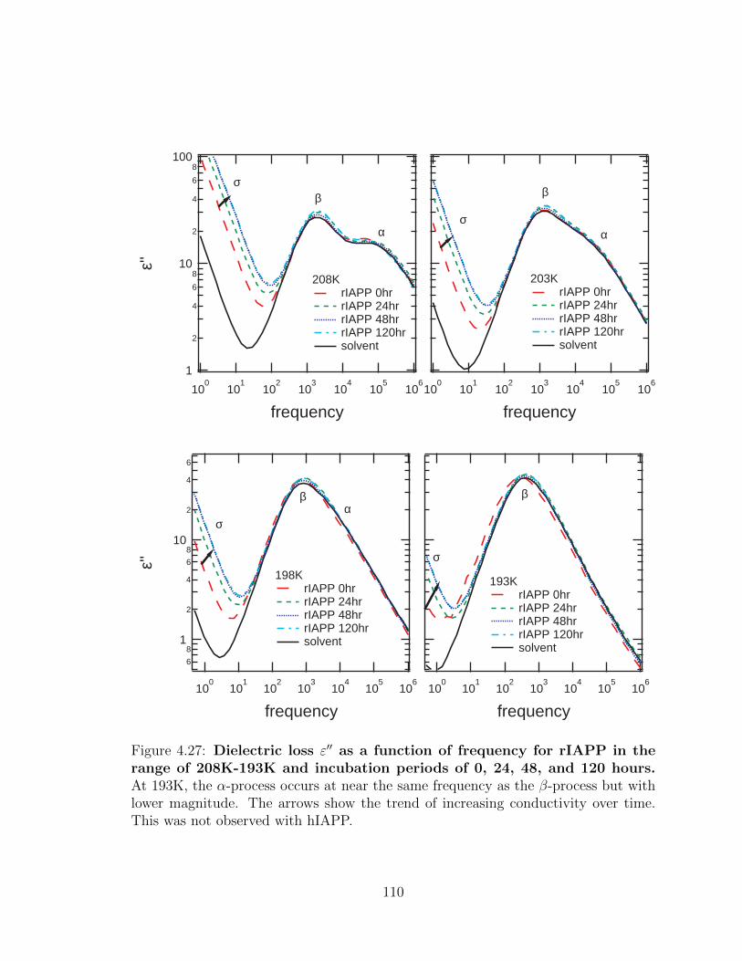
100
101
102
103
104
105
106
frequency
203K rIAPP 0hr rIAPP 24hr rIAPP 48hr rIAPP 120hr solvent
1
2
4
6
810
2
4
6
8100
ε''
100
101
102
103
104
105
106
frequency
208K rIAPP 0hr rIAPP 24hr rIAPP 48hr rIAPP 120hr solvent
100
101
102
103
104
105
106
frequency
193K rIAPP 0hr rIAPP 24hr rIAPP 48hr rIAPP 120hr solvent
6
81
2
4
6
810
2
4
6
ε''
100
101
102
103
104
105
106
frequency
198K rIAPP 0hr rIAPP 24hr rIAPP 48hr rIAPP 120hr solvent
σ
σ
σ
σ
β β
β βα
αα
Figure 4.27: Dielectric loss ε′′ as a function of frequency for rIAPP in therange of 208K-193K and incubation periods of 0, 24, 48, and 120 hours.At 193K, the α-process occurs at near the same frequency as the β-process but withlower magnitude. The arrows show the trend of increasing conductivity over time.This was not observed with hIAPP.
110
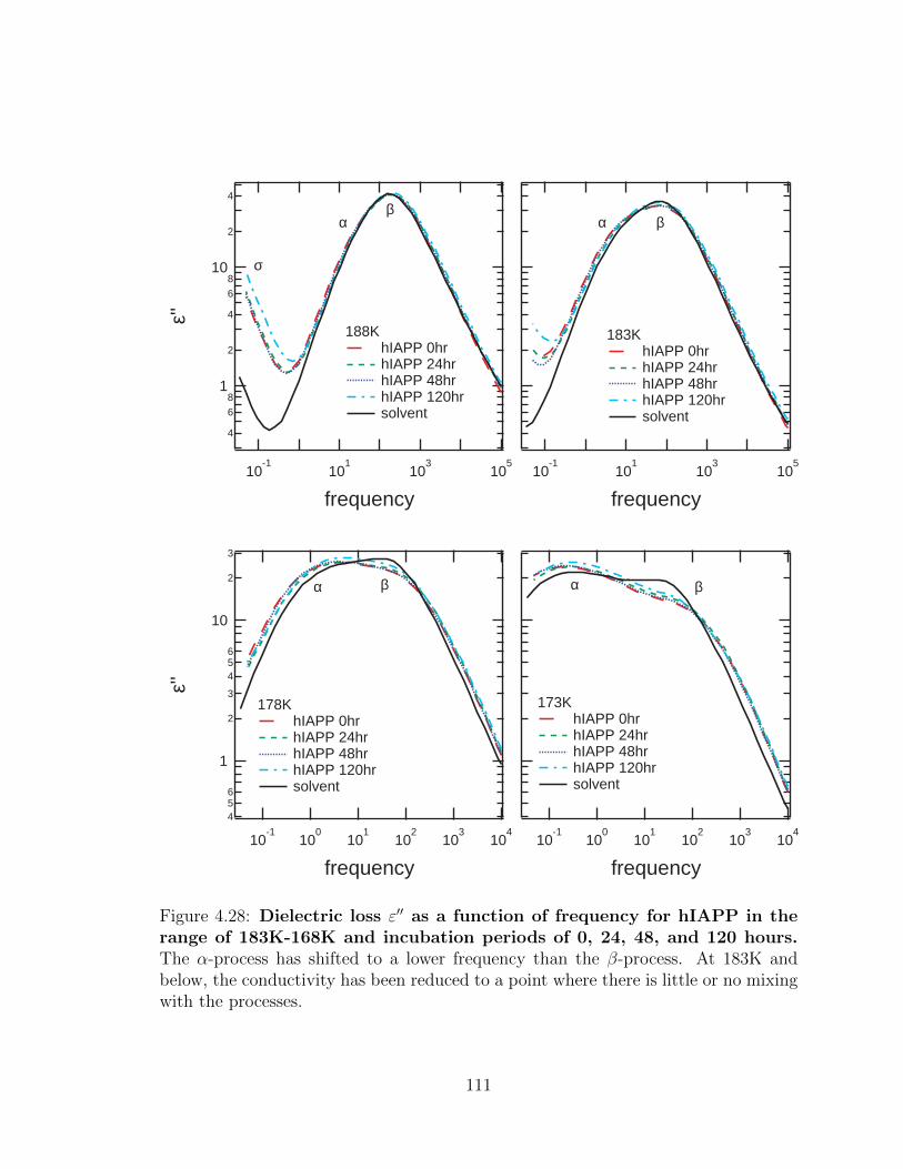
10-1 10
1 103 10
5
frequency
183K hIAPP 0hr hIAPP 24hr hIAPP 48hr hIAPP 120hr solvent
456
1
2
3
456
10
2
3
ε''
10-1
100
101
102
103
104
frequency
178K hIAPP 0hr hIAPP 24hr hIAPP 48hr hIAPP 120hr solvent
10-1
100
101
102
103
104
frequency
173K hIAPP 0hr hIAPP 24hr hIAPP 48hr hIAPP 120hr solvent
4
6
81
2
4
6
810
2
4
ε''
10-1 10
1 103 10
5
frequency
188K hIAPP 0hr hIAPP 24hr hIAPP 48hr hIAPP 120hr solvent
σ
ββ
β βαα
αα
Figure 4.28: Dielectric loss ε′′ as a function of frequency for hIAPP in therange of 183K-168K and incubation periods of 0, 24, 48, and 120 hours.The α-process has shifted to a lower frequency than the β-process. At 183K andbelow, the conductivity has been reduced to a point where there is little or no mixingwith the processes.
111
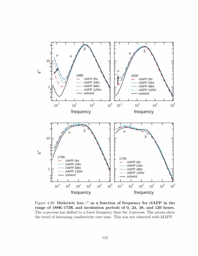
4
6
81
2
4
6
810
2
4
ε''
10-1 10
1 103 10
5
frequency
188K rIAPP 0hr rIAPP 24hr rIAPP 48hr rIAPP 120hr solvent
10-1 10
1 103 10
5
frequency
183K rIAPP 0hr rIAPP 24hr rIAPP 48hr rIAPP 120hr solvent
10-1
100
101
102
103
104
frequency
173K rIAPP 0hr rIAPP 24hr rIAPP 48hr rIAPP 120hr solvent
456
1
2
3
456
10
2
3
ε''
10-1
100
101
102
103
104
frequency
178K rIAPP 0hr rIAPP 24hr rIAPP 48hr rIAPP 120hr solvent
σ
σ
ββ
β
β
αα
αα
Figure 4.29: Dielectric loss ε′′ as a function of frequency for rIAPP in therange of 188K-173K and incubation periods of 0, 24, 48, and 120 hours.The α-process has shifted to a lower frequency than the β-process. The arrows showthe trend of increasing conductivity over time. This was not observed with hIAPP.
112
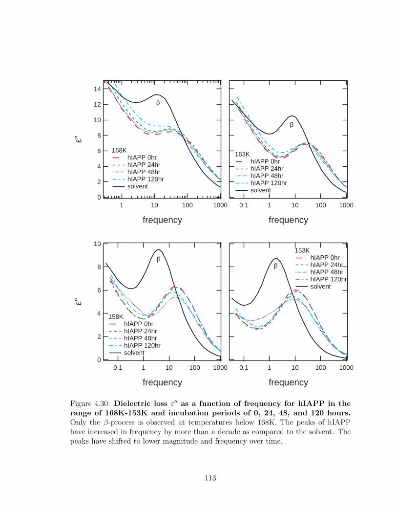
0.1 1 10 100 1000
frequency
153K hIAPP 0hr hIAPP 24hr hIAPP 48hr hIAPP 120hr solvent
10
8
6
4
2
0
ε''
0.1 1 10 100 1000
frequency
158K hIAPP 0hr hIAPP 24hr hIAPP 48hr hIAPP 120hr solvent
0.1 1 10 100 1000
frequency
163K hIAPP 0hr hIAPP 24hr hIAPP 48hr hIAPP 120hr solvent
14
12
10
8
6
4
2
0
ε''
1 10 100 1000
frequency
168K hIAPP 0hr hIAPP 24hr hIAPP 48hr hIAPP 120hr solvent
β
β
ββ
Figure 4.30: Dielectric loss ε′′ as a function of frequency for hIAPP in therange of 168K-153K and incubation periods of 0, 24, 48, and 120 hours.Only the β-process is observed at temperatures below 168K. The peaks of hIAPPhave increased in frequency by more than a decade as compared to the solvent. Thepeaks have shifted to lower magnitude and frequency over time.
113

10
8
6
4
2
0
ε''
0.1 1 10 100 1000
frequency
158K rIAPP 0hr rIAPP 24hr rIAPP 48hr rIAPP 120hr solvent
0.1 1 10 100 1000
frequency
153K rIAPP 0hr rIAPP 24hr rIAPP 48hr rIAPP 120hr solvent
0.1 1 10 100 1000
frequency
163K rIAPP 0hr rIAPP 24hr rIAPP 48hr rIAPP 120hr solvent
14
12
10
8
6
4
2
0
ε''
1 10 100 1000
frequency
168K rIAPP 0hr rIAPP 24hr rIAPP 48hr rIAPP 120hr solvent
β
β
ββ
σ
σ
σ
Figure 4.31: Dielectric loss ε′′ as a function of frequency for rIAPP in therange of 168K-153K and incubation periods of 0, 24, 48, and 120 hours.Only the β-process is observed at temperatures below 158K. The arrows show thatthe conductivity increases and the β-process peaks shift to higher magnitude overtime. This opposite the behavior of hIAPP in the same temperature range. There isno increase in frequency at t = 0hr, where hIAPP displayed a decade shift. The shiftin peak position at 168K and 163K may be due to conductivity.
114
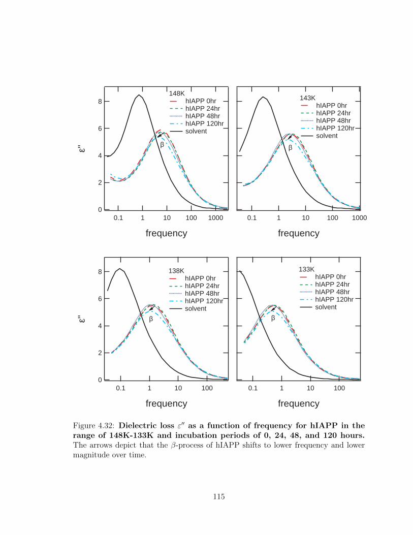
0.1 1 10 100
frequency
133K hIAPP 0hr hIAPP 24hr hIAPP 48hr hIAPP 120hr solvent
8
6
4
2
0
ε''
0.1 1 10 100
frequency
138K hIAPP 0hr hIAPP 24hr hIAPP 48hr hIAPP 120hr solvent
0.1 1 10 100 1000
frequency
143K hIAPP 0hr hIAPP 24hr hIAPP 48hr hIAPP 120hr solvent
8
6
4
2
0
ε''
0.1 1 10 100 1000
frequency
148K hIAPP 0hr hIAPP 24hr hIAPP 48hr hIAPP 120hr solvent
β β
β β
Figure 4.32: Dielectric loss ε′′ as a function of frequency for hIAPP in therange of 148K-133K and incubation periods of 0, 24, 48, and 120 hours.The arrows depict that the β-process of hIAPP shifts to lower frequency and lowermagnitude over time.
115
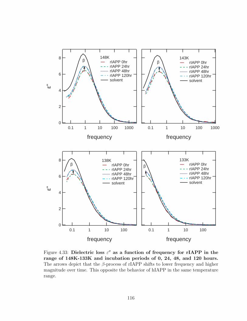
0.1 1 10 100 1000
frequency
143K rIAPP 0hr rIAPP 24hr rIAPP 48hr rIAPP 120hr solvent
8
6
4
2
0
ε''
0.1 1 10 100 1000
frequency
148K rIAPP 0hr rIAPP 24hr rIAPP 48hr rIAPP 120hr solvent
0.1 1 10 100
frequency
133K rIAPP 0hr rIAPP 24hr rIAPP 48hr rIAPP 120hr solvent
8
6
4
2
0
ε''
0.1 1 10 100
frequency
138K rIAPP 0hr rIAPP 24hr rIAPP 48hr rIAPP 120hr solvent
β β
β β
Figure 4.33: Dielectric loss ε′′ as a function of frequency for rIAPP in therange of 148K-133K and incubation periods of 0, 24, 48, and 120 hours.The arrows depict that the β-process of rIAPP shifts to lower frequency and highermagnitude over time. This opposite the behavior of hIAPP in the same temperaturerange.
116
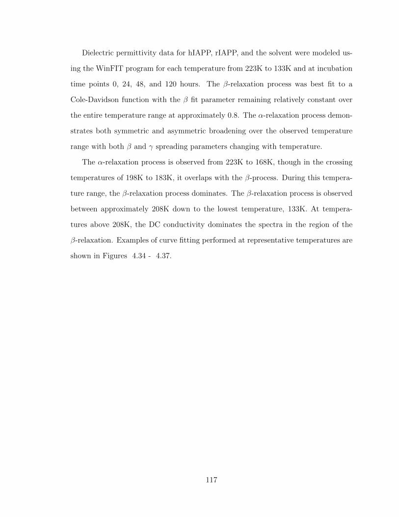
Dielectric permittivity data for hIAPP, rIAPP, and the solvent were modeled us-
ing the WinFIT program for each temperature from 223K to 133K and at incubation
time points 0, 24, 48, and 120 hours. The β-relaxation process was best fit to a
Cole-Davidson function with the β fit parameter remaining relatively constant over
the entire temperature range at approximately 0.8. The α-relaxation process demon-
strates both symmetric and asymmetric broadening over the observed temperature
range with both β and γ spreading parameters changing with temperature.
The α-relaxation process is observed from 223K to 168K, though in the crossing
temperatures of 198K to 183K, it overlaps with the β-process. During this tempera-
ture range, the β-relaxation process dominates. The β-relaxation process is observed
between approximately 208K down to the lowest temperature, 133K. At tempera-
tures above 208K, the DC conductivity dominates the spectra in the region of the
β-relaxation. Examples of curve fitting performed at representative temperatures are
shown in Figures 4.34 - 4.37.
117
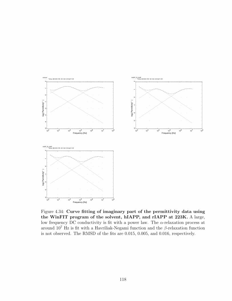
102
103
104
105
106
107
108
Frequency [Hz]
-5-4
-3-2
-10
12
log( Perm
ittivity'' )
solvent Temp. [K]=223.150 AC Volt [Vrms]=1.00
102
103
104
105
106
107
108
Frequency [Hz]-4
-3-2
-10
12
log( Perm
ittivity'' )
hIAPP_DI_0HR Temp. [K]=223.150 AC Volt [Vrms]=1.00
102
103
104
105
106
107
108
Frequency [Hz]
-4-3
-2-1
01
2
log( Perm
ittivity'' )
rIAPP_DI_0HR Temp. [K]=223.150 AC Volt [Vrms]=1.00
Figure 4.34: Curve fitting of imaginary part of the permittivity data usingthe WinFIT program of the solvent, hIAPP, and rIAPP at 223K. A large,low frequency DC conductivity is fit with a power law. The α-relaxation process ataround 107 Hz is fit with a Havriliak-Negami function and the β-relaxation functionis not observed. The RMSD of the fits are 0.015, 0.005, and 0.016, respectively.
118

100
101
102
103
104
105
106
107
Frequency [Hz]
-6-4
-20
2
log
( P
erm
itti
vit
y''
)
solvent Temp. [K]=208.150 AC Volt [Vrms]=1.00
100
101
102
103
104
105
106
107
Frequency [Hz]
-5-4
-3-2
-10
12
log
( P
erm
itti
vit
y''
)
hIAPP_DI_0HR Temp. [K]=208.150 AC Volt [Vrms]=1.00
100
101
102
103
104
105
106
107
Frequency [Hz]
-4-3
-2-1
01
2
log
( P
erm
itti
vit
y''
)
rIAPP_DI_0HR Temp. [K]=208.150 AC Volt [Vrms]=1.00
Figure 4.35: Curve fitting of imaginary part of the permittivity data usingthe WinFIT program of the solvent, hIAPP, and rIAPP at 208K. A large,low frequency DC conductivity is fit with a power law. The β-relaxation process ataround 103 Hz is fit with a Cole-Davidson function and the α-relaxation process ataround 105 Hz is fit with a Havriliak-Negami function. The RMSD of the fits are0.027, 0.013, and 0.010, respectively.
119

10-1
100
101
102
103
104
105
106
Frequency [Hz]
-8-6
-4-2
02
4
log
( P
erm
itti
vit
y''
)
solvent Temp. [K]=188.150 AC Volt [Vrms]=1.00
10-1
100
101
102
103
104
105
106
Frequency [Hz]
-8-6
-4-2
02
4
log
( P
erm
itti
vit
y''
)
hIAPP_DI_0HR Temp. [K]=188.150 AC Volt [Vrms]=1.00
10-2
10-1
100
101
102
103
104
105
Frequency [Hz]
-5-4
-3-2
-10
12
log( Permittivity'' )
RIAPP_DI_0HR Temp. [K]=188.150 AC Volt [Vrms]=1.00
Figure 4.36: Curve fitting of imaginary part of the permittivity data usingthe WinFIT program of the solvent, hIAPP, and rIAPP at 188K. A large,low frequency DC conductivity is fit with a power law. The β-relaxation processat around 103 Hz is fit with a Cole-Davidson function and the α-relaxation processat around 101 Hz is fit with a Havriliak-Negami function. Here, the α process hascrossed over to slower than β relaxation times. The RMSD of the fits are 0.012, 0.004,and 0.043, respectively.
120
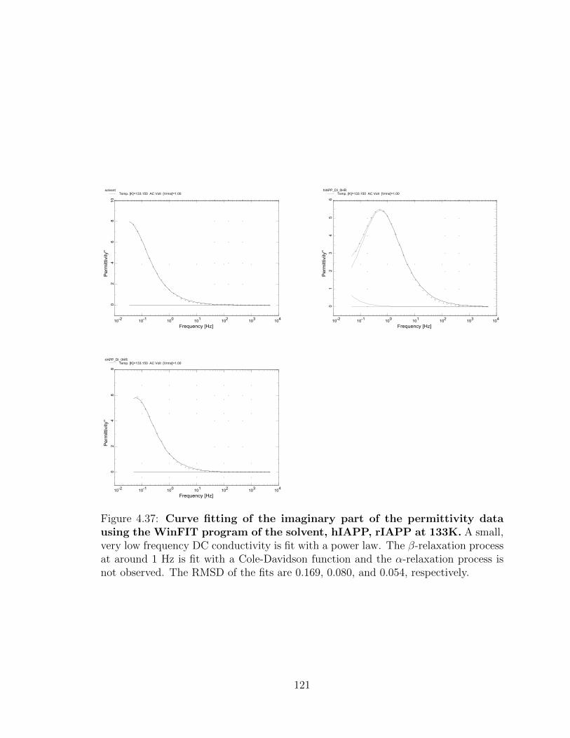
10-2
10-1
100
101
102
103
104
Frequency [Hz]
02
46
810
Perm
ittivity''
solvent Temp. [K]=133.150 AC Volt [Vrms]=1.00
10-2
10-1
100
101
102
103
104
Frequency [Hz]0
12
34
56
Permittivity''
hIAPP_DI_0HR Temp. [K]=133.150 AC Volt [Vrms]=1.00
10-2
10-1
100
101
102
103
104
Frequency [Hz]
02
46
8
Permittivity''
rIAPP_DI_0HR Temp. [K]=133.150 AC Volt [Vrms]=1.00
Figure 4.37: Curve fitting of the imaginary part of the permittivity datausing the WinFIT program of the solvent, hIAPP, rIAPP at 133K. A small,very low frequency DC conductivity is fit with a power law. The β-relaxation processat around 1 Hz is fit with a Cole-Davidson function and the α-relaxation process isnot observed. The RMSD of the fits are 0.169, 0.080, and 0.054, respectively.
121

The maximum frequency, fmax of ε′′ of both the α- and β-relaxation processes
were determined from the model function curve fitting of the permittivity data at
all temperatures. Arrhenius plots of fmax versus inverse temperature, 1000/T were
created for each process. The β-relaxation process follows a linear, or Arrhenius
behavior throughout the temperature range. The α-relaxation process follows a slight
non-linear Vogel-Fulcher-Tammann (VFT)-type behavior that is expected in glass-
forming solvents such as glycerol (Figures 4.38 - 4.40). Activation energies for the
β process and glass-forming fragilities for the α process were determined from the
Arrhenius and VFT analysis and displayed in Tables 4.3 and 4.4. The activation
energies for hIAPP matches the value of 24.4 kJ/mol obtained by Knowles et al. from
measurements using the quartz crystal microbalance (QCM) method [155].
6
4
2
0
log(
f max
)
7.57.06.56.05.55.04.5
1000/T
solvent
Figure 4.38: Arrhenius plots of fmax versus inverse temperature for sol-vent over time. The α-relaxation process follows a VFT behavior whereas theβ-relaxation process follows an Arrhenius, or linear behavior.
The structure of hIAPP has been shown by FTIR and NMR to display both
parallel and anti-parallel β-sheets [156, 157]. Figure 4.41 shows that over time,
hIAPP displayed a series of increases and decreases in the dielectric strength as fibril
122
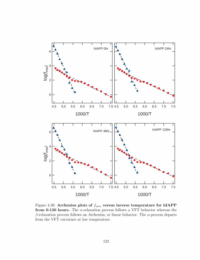
7.57.06.56.05.55.04.5
1000/T
hIAPP 120hr
6
4
2
0
log(
f max
)
7.57.06.56.05.55.04.5
1000/T
hIAPP 0hr
6
4
2
0
log(
f max
)
7.57.06.56.05.55.04.5
1000/T
hIAPP 48hr
7.57.06.56.05.55.04.5
1000/T
hIAPP 24hr
Figure 4.39: Arrhenius plots of fmax versus inverse temperature for hIAPPfrom 0-120 hours. The α-relaxation process follows a VFT behavior whereas theβ-relaxation process follows an Arrhenius, or linear behavior. The α-process departsfrom the VFT curvature at low temperature.
123
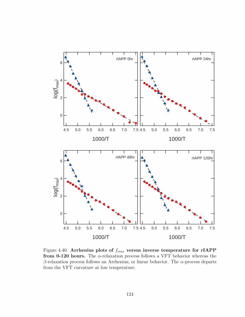
7.57.06.56.05.55.04.5
1000/T
rIAPP 120hr
7.57.06.56.05.55.04.5
1000/T
rIAPP 24hr6
4
2
0
log(
f max
)
7.57.06.56.05.55.04.5
1000/T
rIAPP 0hr
6
4
2
0
log(
f max
)
7.57.06.56.05.55.04.5
1000/T
rIAPP 48hr
Figure 4.40: Arrhenius plots of fmax versus inverse temperature for rIAPPfrom 0-120 hours. The α-relaxation process follows a VFT behavior whereas theβ-relaxation process follows an Arrhenius, or linear behavior. The α-process departsfrom the VFT curvature at low temperature.
124

EA EAtime A B (kJ/mol) time A B (kJ/mol)
hIAPP
0hr 9.25 1.269 24.3
rIAPP
0hr 10.62 1.541 29.524hr 9.09 1.229 23.5 24hr 11.3 1.658 31.748hr 9.29 1.273 24.4 48hr 11.4 1.696 32.4120hr 9.28 1.266 24.2 120hr 11.3 1.680 32.2
solvent 11.2 1.646 31.5 solvent 11.2 1.646 31.5
Table 4.3: Parameters of the linear fits to the β-relaxation measurements oflog(fmax(T )) of the form A+BT .
time logf∞ D T0 (K) time logf∞ D T0 (K)
hIAPP
0hr 22 30 75
rIAPP
0hr 22 36 6724hr 22 36 67 24hr 22 37 6648hr 22 33 71 48hr 22 37 66120hr 22 34 70 120hr 22 37 67
solvent 22 33 70 solvent 22 33 70
Table 4.4: Parameters of the VFT fits to the α-relaxation measurements of fmax(T )of the form log(fmax) = log(f∞(T ))− DT0
T−T0
formation progresses, whereas the non-amyloidogenic rIAPP increased consistently
over time. The increase and decrease cycles for hIAPP may be due to a mixture of
both parallel and anti-parallel β-sheet conformations dominating at different phases
of the aggregation process. The continuing increase of dipole moment for random-coil
aggregation is an explanation for the increasing dielectric strength in rIAPP.
125
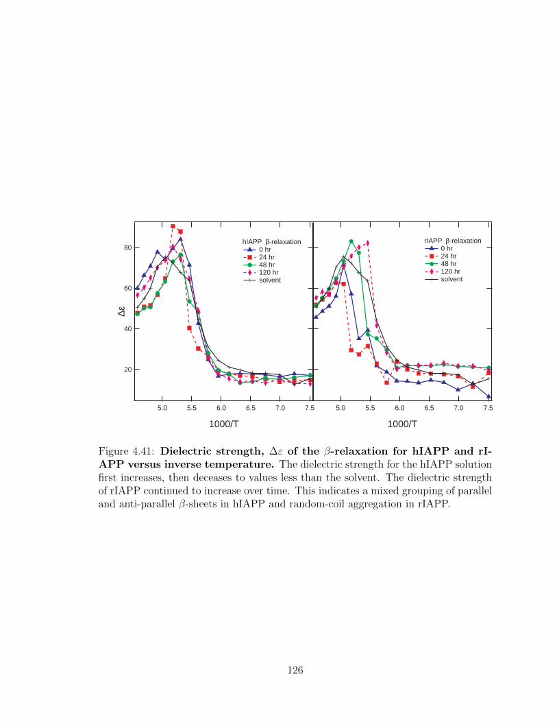
7.57.06.56.05.55.0
1000/T
rIAPP β-relaxation 0 hr 24 hr 48 hr 120 hr solvent
80
60
40
20
∆ε
7.57.06.56.05.55.0
1000/T
hIAPP β-relaxation 0 hr 24 hr 48 hr 120 hr solvent
Figure 4.41: Dielectric strength, ∆ε of the β-relaxation for hIAPP and rI-APP versus inverse temperature. The dielectric strength for the hIAPP solutionfirst increases, then deceases to values less than the solvent. The dielectric strengthof rIAPP continued to increase over time. This indicates a mixed grouping of paralleland anti-parallel β-sheets in hIAPP and random-coil aggregation in rIAPP.
126
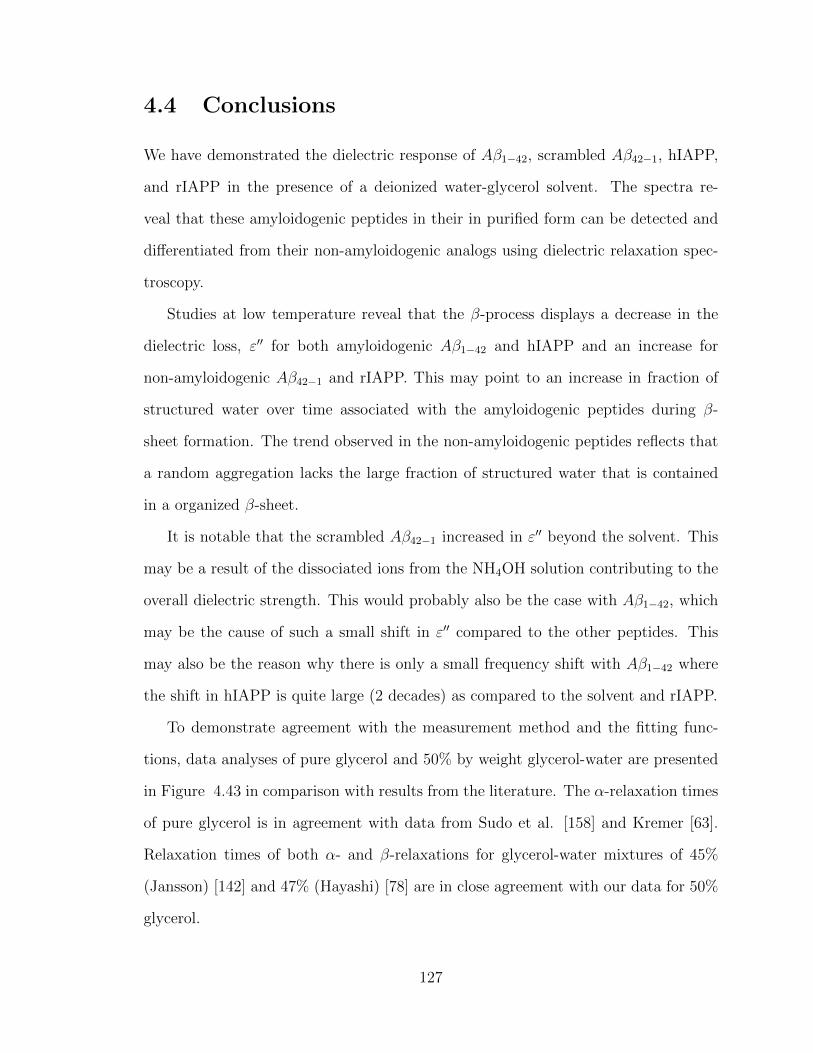
4.4 Conclusions
We have demonstrated the dielectric response of Aβ1−42, scrambled Aβ42−1, hIAPP,
and rIAPP in the presence of a deionized water-glycerol solvent. The spectra re-
veal that these amyloidogenic peptides in their in purified form can be detected and
differentiated from their non-amyloidogenic analogs using dielectric relaxation spec-
troscopy.
Studies at low temperature reveal that the β-process displays a decrease in the
dielectric loss, ε′′ for both amyloidogenic Aβ1−42 and hIAPP and an increase for
non-amyloidogenic Aβ42−1 and rIAPP. This may point to an increase in fraction of
structured water over time associated with the amyloidogenic peptides during β-
sheet formation. The trend observed in the non-amyloidogenic peptides reflects that
a random aggregation lacks the large fraction of structured water that is contained
in a organized β-sheet.
It is notable that the scrambled Aβ42−1 increased in ε′′ beyond the solvent. This
may be a result of the dissociated ions from the NH4OH solution contributing to the
overall dielectric strength. This would probably also be the case with Aβ1−42, which
may be the cause of such a small shift in ε′′ compared to the other peptides. This
may also be the reason why there is only a small frequency shift with Aβ1−42 where
the shift in hIAPP is quite large (2 decades) as compared to the solvent and rIAPP.
To demonstrate agreement with the measurement method and the fitting func-
tions, data analyses of pure glycerol and 50% by weight glycerol-water are presented
in Figure 4.43 in comparison with results from the literature. The α-relaxation times
of pure glycerol is in agreement with data from Sudo et al. [158] and Kremer [63].
Relaxation times of both α- and β-relaxations for glycerol-water mixtures of 45%
(Jansson) [142] and 47% (Hayashi) [78] are in close agreement with our data for 50%
glycerol.
127

3x100
4
5
6
ε''
4 5 60.1
2 3 4 5 61
2 3 4 5 610
2
frequency
Aβ1-42 0hr Aβ1-42 24hr Aβ42-1 0hr Aβ42-1 24hr solvent
3x100
4
5
6
7
8
9
ε''
4 5 60.1
2 3 4 5 61
2 3 4 5 610
2
frequency
hIAPP 0hr hIAPP 120 hr rIAPP 0hr rIAPP 120hr solvent
Figure 4.42: Plots of the β-relaxation peak shift at 143K for Aβ1−42/Aβ42−1 andhIAPP/rIAPP as compared to the solvent.
128
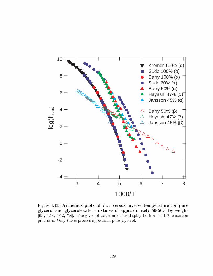
10
8
6
4
2
0
-2
-4
log(
f max
)
876543
1000/T
Kremer 100% (α) Sudo 100% (α) Barry 100% (α) Sudo 60% (α) Barry 50% (α) Hayashi 47% (α) Jansson 45% (α)
Barry 50% (β) Hayashi 47% (β) Jansson 45% (β)
Figure 4.43: Arrhenius plots of fmax versus inverse temperature for pureglycerol and glycerol-water mixtures of approximately 50-50% by weight[63, 158, 142, 78]. The glycerol-water mixtures display both α- and β-relaxationprocesses. Only the α process appears in pure glycerol.
129
In Table 4.5, we present activation energies from a selection of small, aggregating
peptides in solution. These include silk fibroin [130], Aβ1−40 [149], chymotrypsin
inhibitor 2 (CI2) [149, 159], phage λ repressor [149, 160, 161], SH3 domain of spectrin
[149, 162, 163], the C-terminal fragment(4156) from protein GB1 [149, 164], and
insulin [155]. Interestingly, the activation energies for these peptides are within the
same order of magnitude, yet each have a distinctive value.
peptide EA (kJ/mol) structure
silk fibroin 27 α,βAβ1−40 23 βCI2 31.2 α,βλ repressor 16.1 αSH3 9.5 βGB1 11.6 β-hairpininsulin 24.4 β
Table 4.5: Activation energies for various small, aggregating peptides
Studies of the dielectric strength over a range of temperatures and incubation
times show that determination of β-sheet conformation by dielectric spectroscopy is
in agreement with previous studies done using FTIR and solid state NMR. The Aβ1−42
displayed anti-parallel characteristics and the hIAPP displayed both parallel and anti-
parallel signatures. The non-amyloidogenic peptides produced dipole moments that
would be consistent with random coil or non-aggregating proteins.
The use of deionized water as a buffer is informative in that the amount of interfer-
ing substances is kept at a minimum. However, deionized water is not representative
of native fluids that harbor amyloidogenic peptides. A continuation of this work in
bovine serum albumin (BSA) will aid in simulation of more in vivo-like conditions.
This also may provide a more favorable environment for aggregation and bring the
analysis closer to realistic, diagnostic conditions. Additionally, exclusion of NH4OH
in the study of Aβ1−42 and scrambled Aβ42−1 should be explored.
130
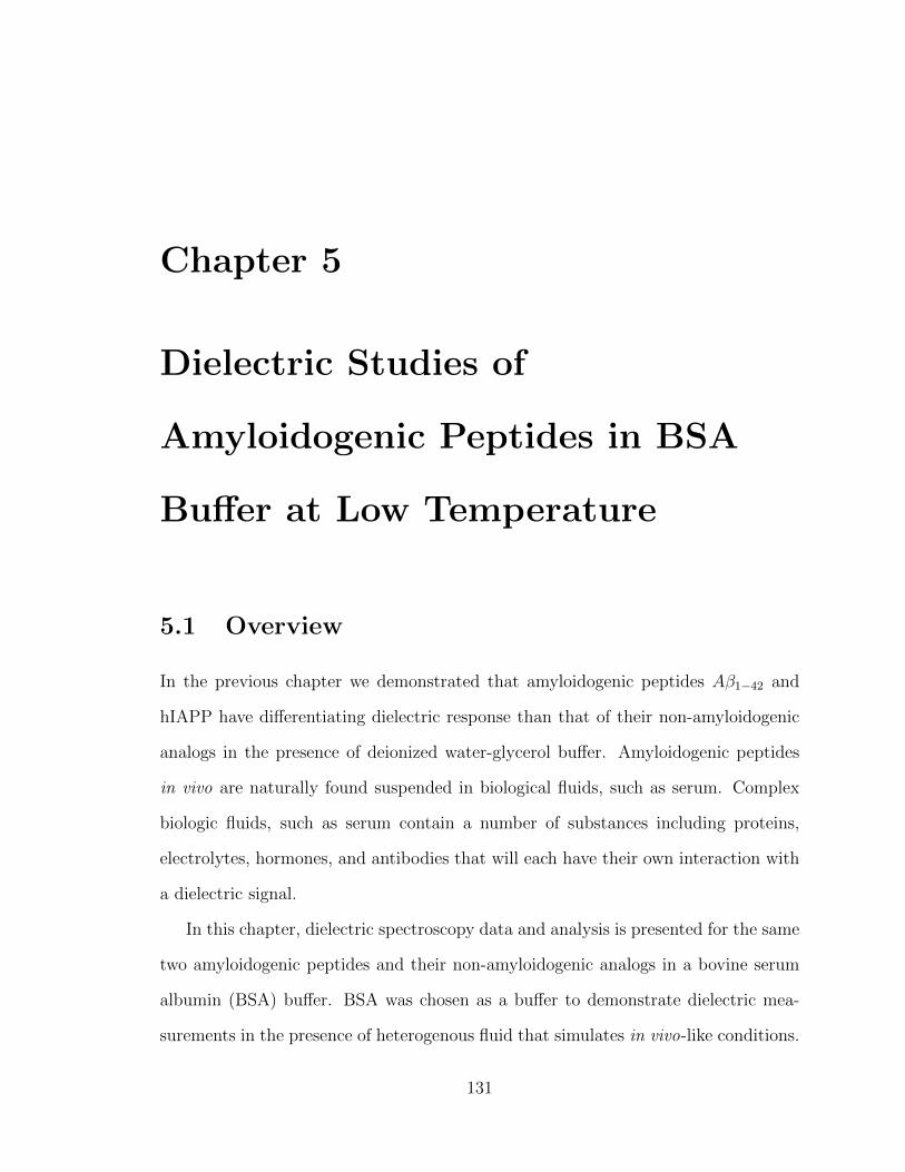
Chapter 5
Dielectric Studies of
Amyloidogenic Peptides in BSA
Buffer at Low Temperature
5.1 Overview
In the previous chapter we demonstrated that amyloidogenic peptides Aβ1−42 and
hIAPP have differentiating dielectric response than that of their non-amyloidogenic
analogs in the presence of deionized water-glycerol buffer. Amyloidogenic peptides
in vivo are naturally found suspended in biological fluids, such as serum. Complex
biologic fluids, such as serum contain a number of substances including proteins,
electrolytes, hormones, and antibodies that will each have their own interaction with
a dielectric signal.
In this chapter, dielectric spectroscopy data and analysis is presented for the same
two amyloidogenic peptides and their non-amyloidogenic analogs in a bovine serum
albumin (BSA) buffer. BSA was chosen as a buffer to demonstrate dielectric mea-
surements in the presence of heterogenous fluid that simulates in vivo-like conditions.
131
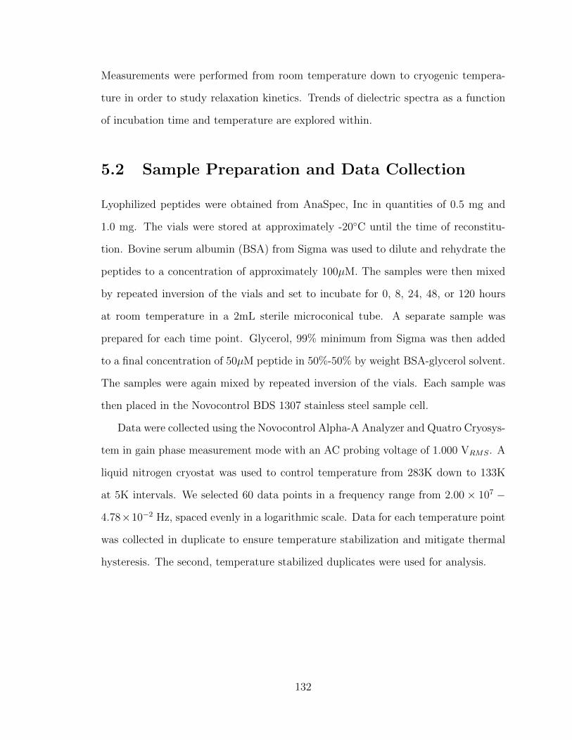
Measurements were performed from room temperature down to cryogenic tempera-
ture in order to study relaxation kinetics. Trends of dielectric spectra as a function
of incubation time and temperature are explored within.
5.2 Sample Preparation and Data Collection
Lyophilized peptides were obtained from AnaSpec, Inc in quantities of 0.5 mg and
1.0 mg. The vials were stored at approximately -20C until the time of reconstitu-
tion. Bovine serum albumin (BSA) from Sigma was used to dilute and rehydrate the
peptides to a concentration of approximately 100µM. The samples were then mixed
by repeated inversion of the vials and set to incubate for 0, 8, 24, 48, or 120 hours
at room temperature in a 2mL sterile microconical tube. A separate sample was
prepared for each time point. Glycerol, 99% minimum from Sigma was then added
to a final concentration of 50µM peptide in 50%-50% by weight BSA-glycerol solvent.
The samples were again mixed by repeated inversion of the vials. Each sample was
then placed in the Novocontrol BDS 1307 stainless steel sample cell.
Data were collected using the Novocontrol Alpha-A Analyzer and Quatro Cryosys-
tem in gain phase measurement mode with an AC probing voltage of 1.000 VRMS. A
liquid nitrogen cryostat was used to control temperature from 283K down to 133K
at 5K intervals. We selected 60 data points in a frequency range from 2.00 × 10⁷ −
4.78×10⁻² Hz, spaced evenly in a logarithmic scale. Data for each temperature point
was collected in duplicate to ensure temperature stabilization and mitigate thermal
hysteresis. The second, temperature stabilized duplicates were used for analysis.
132
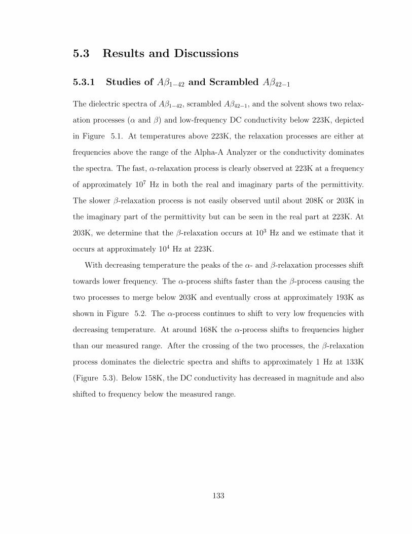
5.3 Results and Discussions
5.3.1 Studies of Aβ1−42 and Scrambled Aβ42−1
The dielectric spectra of Aβ1−42, scrambled Aβ42−1, and the solvent shows two relax-
ation processes (α and β) and low-frequency DC conductivity below 223K, depicted
in Figure 5.1. At temperatures above 223K, the relaxation processes are either at
frequencies above the range of the Alpha-A Analyzer or the conductivity dominates
the spectra. The fast, α-relaxation process is clearly observed at 223K at a frequency
of approximately 107 Hz in both the real and imaginary parts of the permittivity.
The slower β-relaxation process is not easily observed until about 208K or 203K in
the imaginary part of the permittivity but can be seen in the real part at 223K. At
203K, we determine that the β-relaxation occurs at 103 Hz and we estimate that it
occurs at approximately 104 Hz at 223K.
With decreasing temperature the peaks of the α- and β-relaxation processes shift
towards lower frequency. The α-process shifts faster than the β-process causing the
two processes to merge below 203K and eventually cross at approximately 193K as
shown in Figure 5.2. The α-process continues to shift to very low frequencies with
decreasing temperature. At around 168K the α-process shifts to frequencies higher
than our measured range. After the crossing of the two processes, the β-relaxation
process dominates the dielectric spectra and shifts to approximately 1 Hz at 133K
(Figure 5.3). Below 158K, the DC conductivity has decreased in magnitude and also
shifted to frequency below the measured range.
133
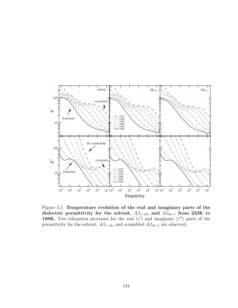
4
6
810
2
4
6
8100
2
ε''
102
103
104
105
106
107
102
103
104
105
106
107
frequency
223K 218K 213K 208K 203K 198K
102
103
104
105
106
107
4
6
810
2
4
6
8100
2
ε'
223K 218K 213K 208K 203K 198K
Aβ1-42 Aβ42-1solvent
α-process
β-process
α-process
β-process
DC conductivity
Figure 5.1: Temperature evolution of the real and imaginary parts of thedielectric permittivity for the solvent, Aβ1−42, and Aβ42−1 from 223K to198K. Two relaxation processes for the real (ε′) and imaginary (ε′′) parts of thepermittivity for the solvent, Aβ1−42, and scrambled Aβ42−1 are observed.
134

456
10
2
3
456
100
2
ε'
1
10
100
1000
ε''
10-1 10
1 103 10
510
-1 101 10
3 105
frequency
193K 188K 183K 178K 173K 168K
10-1 10
1 103 10
5
193K 188K 183K 178K 173K 168K
solvent Aβ1-42 Aβ42-1
β-process
β-process
α-process
α-process
DC conductivity
Figure 5.2: Temperature evolution of the real and imaginary parts of the di-electric permittivity for the solvent,Aβ1−42, and Aβ42−1 from 193K to 168K.The α-relaxation process rapidly shifts to lower frequency with decreasing tempera-ture. In the range of 193K to 188K the two processes cross where the α-relaxation isat lower frequency than the β-relaxation process at temperatures of 183K and below.
135
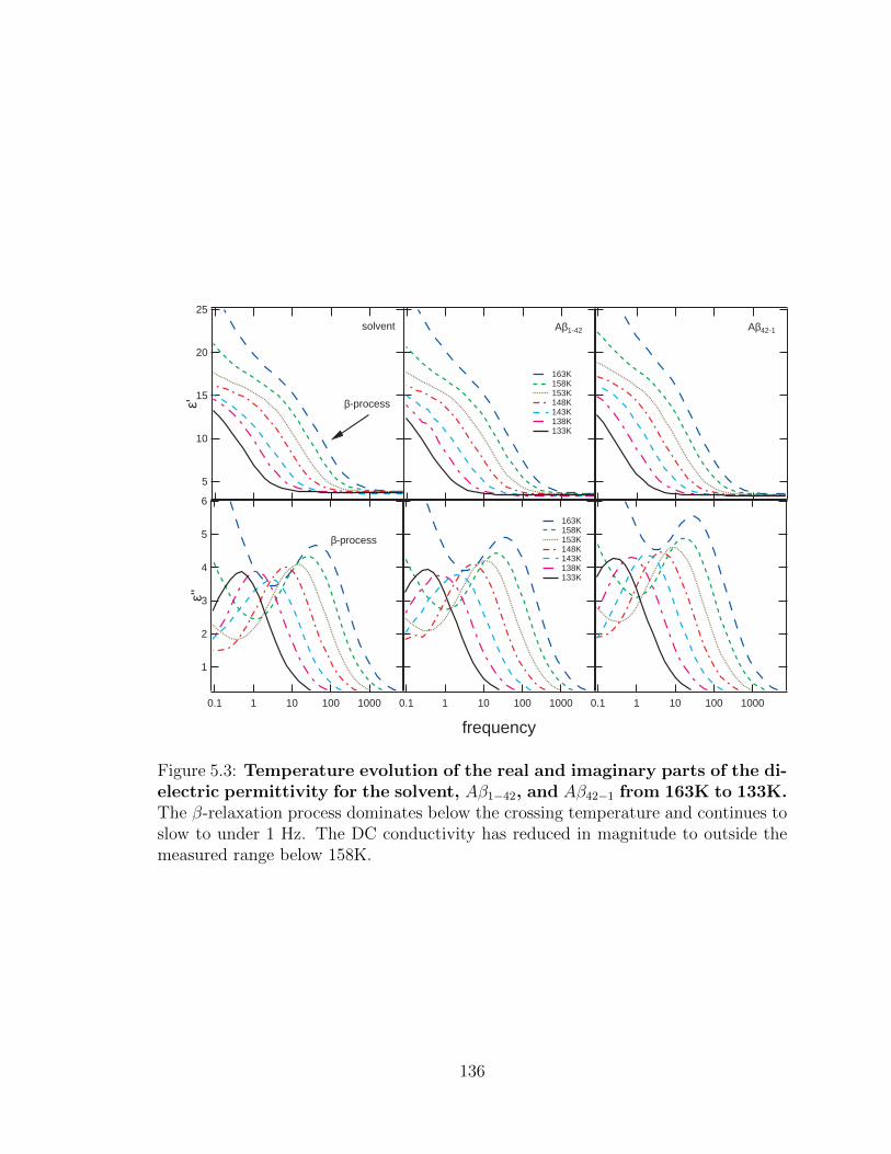
0.1 1 10 100 10000.1 1 10 100 1000
frequency
163K 158K 153K 148K 143K 138K 133K
163K 158K 153K 148K 143K 138K 133K
6
5
4
3
2
1
ε''
0.1 1 10 100 1000
25
20
15
10
5
ε'
solvent Aβ1-42 Aβ42-1
β-process
β-process
Figure 5.3: Temperature evolution of the real and imaginary parts of the di-electric permittivity for the solvent, Aβ1−42, and Aβ42−1 from 163K to 133K.The β-relaxation process dominates below the crossing temperature and continues toslow to under 1 Hz. The DC conductivity has reduced in magnitude to outside themeasured range below 158K.
136
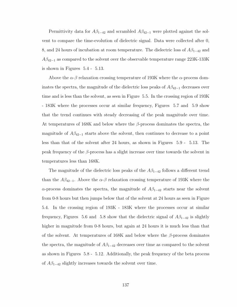
Permittivity data for Aβ1−42 and scrambled Aβ42−1 were plotted against the sol-
vent to compare the time-evolution of dielectric signal. Data were collected after 0,
8, and 24 hours of incubation at room temperature. The dielectric loss of Aβ1−42 and
Aβ42−1 as compared to the solvent over the observable temperature range 223K-133K
is shown in Figures 5.4 - 5.13.
Above the α-β relaxation crossing temperature of 193K where the α-process dom-
inates the spectra, the magnitude of the dielectric loss peaks of Aβ42−1 decreases over
time and is less than the solvent, as seen in Figure 5.5. In the crossing region of 193K
- 183K where the processes occur at similar frequency, Figures 5.7 and 5.9 show
that the trend continues with steady decreasing of the peak magnitude over time.
At temperatures of 168K and below where the β-process dominates the spectra, the
magnitude of Aβ42−1 starts above the solvent, then continues to decrease to a point
less than that of the solvent after 24 hours, as shown in Figures 5.9 - 5.13. The
peak frequency of the β-process has a slight increase over time towards the solvent in
temperatures less than 168K.
The magnitude of the dielectric loss peaks of the Aβ1−42 follows a different trend
than the Aβ42−1. Above the α-β relaxation crossing temperature of 193K where the
α-process dominates the spectra, the magnitude of Aβ1−42 starts near the solvent
from 0-8 hours but then jumps below that of the solvent at 24 hours as seen in Figure
5.4. In the crossing region of 193K - 183K where the processes occur at similar
frequency, Figures 5.6 and 5.8 show that the dielectric signal of Aβ1−42 is slightly
higher in magnitude from 0-8 hours, but again at 24 hours it is much less than that
of the solvent. At temperatures of 168K and below where the β-process dominates
the spectra, the magnitude of Aβ1−42 decreases over time as compared to the solvent
as shown in Figures 5.8 - 5.12. Additionally, the peak frequency of the beta process
of Aβ1−42 slightly increases towards the solvent over time.
137
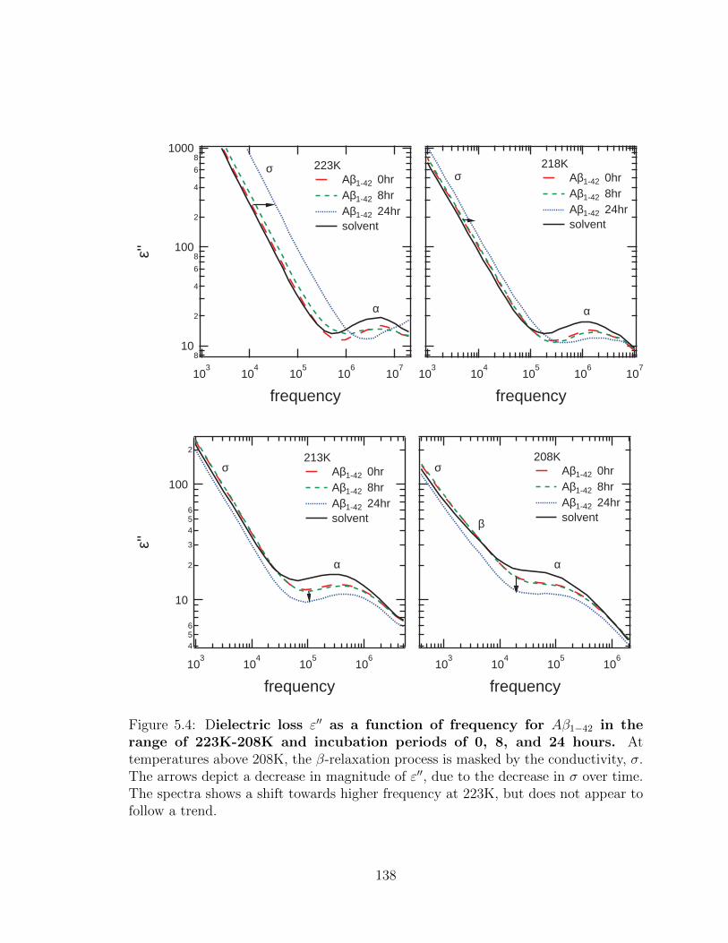
456
10
2
3
456
100
2
ε''
103
104
105
106
frequency
213K Aβ1-42 0hr Aβ1-42 8hr Aβ1-42 24hr solvent
103
104
105
106
107
frequency
218K Aβ1-42 0hr Aβ1-42 8hr Aβ1-42 24hr solvent
103
104
105
106
frequency
208K Aβ1-42 0hr Aβ1-42 8hr Aβ1-42 24hr solvent
810
2
4
6
8100
2
4
6
81000
ε''
103
104
105
106
107
frequency
223K Aβ1-42 0hr Aβ1-42 8hr Aβ1-42 24hr solvent
σσ
σ σ
α α
α α
β
Figure 5.4: Dielectric loss ε′′ as a function of frequency for Aβ1−42 in therange of 223K-208K and incubation periods of 0, 8, and 24 hours. Attemperatures above 208K, the β-relaxation process is masked by the conductivity, σ.The arrows depict a decrease in magnitude of ε′′, due to the decrease in σ over time.The spectra shows a shift towards higher frequency at 223K, but does not appear tofollow a trend.
138
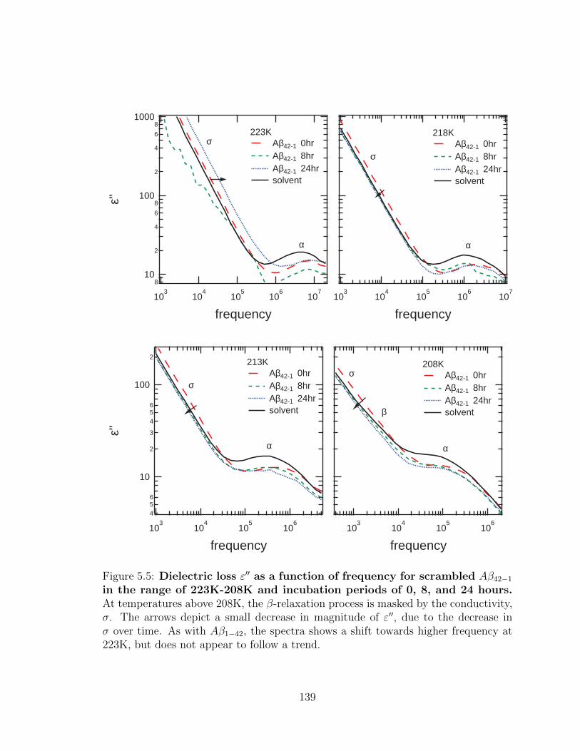
103
104
105
106
frequency
208K Aβ42-1 0hr Aβ42-1 8hr Aβ42-1 24hr solvent
810
2
4
6
8100
2
4
6
81000
ε''
103
104
105
106
107
frequency
223K Aβ42-1 0hr Aβ42-1 8hr Aβ42-1 24hr solvent
456
10
2
3
456
100
2
ε''
103
104
105
106
frequency
213K Aβ42-1 0hr Aβ42-1 8hr Aβ42-1 24hr solvent
103
104
105
106
107
frequency
218K Aβ42-1 0hr Aβ42-1 8hr Aβ42-1 24hr solvent
σ
σ
σσ
αα
αα
β
Figure 5.5: Dielectric loss ε′′ as a function of frequency for scrambled Aβ42−1in the range of 223K-208K and incubation periods of 0, 8, and 24 hours.At temperatures above 208K, the β-relaxation process is masked by the conductivity,σ. The arrows depict a small decrease in magnitude of ε′′, due to the decrease inσ over time. As with Aβ1−42, the spectra shows a shift towards higher frequency at223K, but does not appear to follow a trend.
139

100
101
102
103
104
frequency
188K Aβ1-42 0hr Aβ1-42 8hr Aβ1-42 24hr solvent
2
3
4
56
10
2
3
4
56
100
ε''
101
102
103
104
frequency
193K Aβ1-42 0hr Aβ1-42 8hr Aβ1-42 24hr solvent
6 8
102
2 4 6 8
103
2 4 6 8
104
2 4
frequency
198K Aβ1-42 0hr Aβ1-42 8hr Aβ1-42 24hr solvent
2
3
456
10
2
3
456
100
ε''
102
103
104
105
106
frequency
203K Aβ1-42 0hr Aβ1-42 8hr Aβ1-42 24hr solvent
σσ
σσ
β β
ββ
α
α
α
Figure 5.6: Dielectric loss ε′′ as a function of frequency for Aβ1−42 in therange of 203K-188K and incubation periods of 0, 8, and 24 hours. At 193K,the α-process occurs at near the same frequency as the β-process but with lowermagnitude. The arrows show a shift in magnitude of ε′′ across the spectra due to theconductivity, σ.
140

100
101
102
103
104
frequency
188K Aβ42-1 0hr Aβ42-1 8hr Aβ42-1 24hr solvent
102
103
104
frequency
198K Aβ42-1 0hr Aβ42-1 8hr Aβ42-1 24hr solvent
2
3
456
10
2
3
456
100
ε''
102
103
104
105
106
frequency
203K Aβ42-1 0hr Aβ42-1 8hr Aβ42-1 24hr solvent
2
3
4
56
10
2
3
4
56
100
ε''
101
102
103
104
frequency
193K Aβ42-1 0hr Aβ42-1 8hr Aβ42-1 24hr solvent
σσ
σ σ
ββ
ββ
α
αα
Figure 5.7: Dielectric loss ε′′ as a function of frequency for scrambled Aβ42−1in the range of 203K-188K and incubation periods of 0, 8, and 24 hours.At 193K, the α-process occurs at near the same frequency as the β-process but withlower magnitude. The arrows show a shift in magnitude of ε′′ across the spectra dueto the conductivity, σ.
141
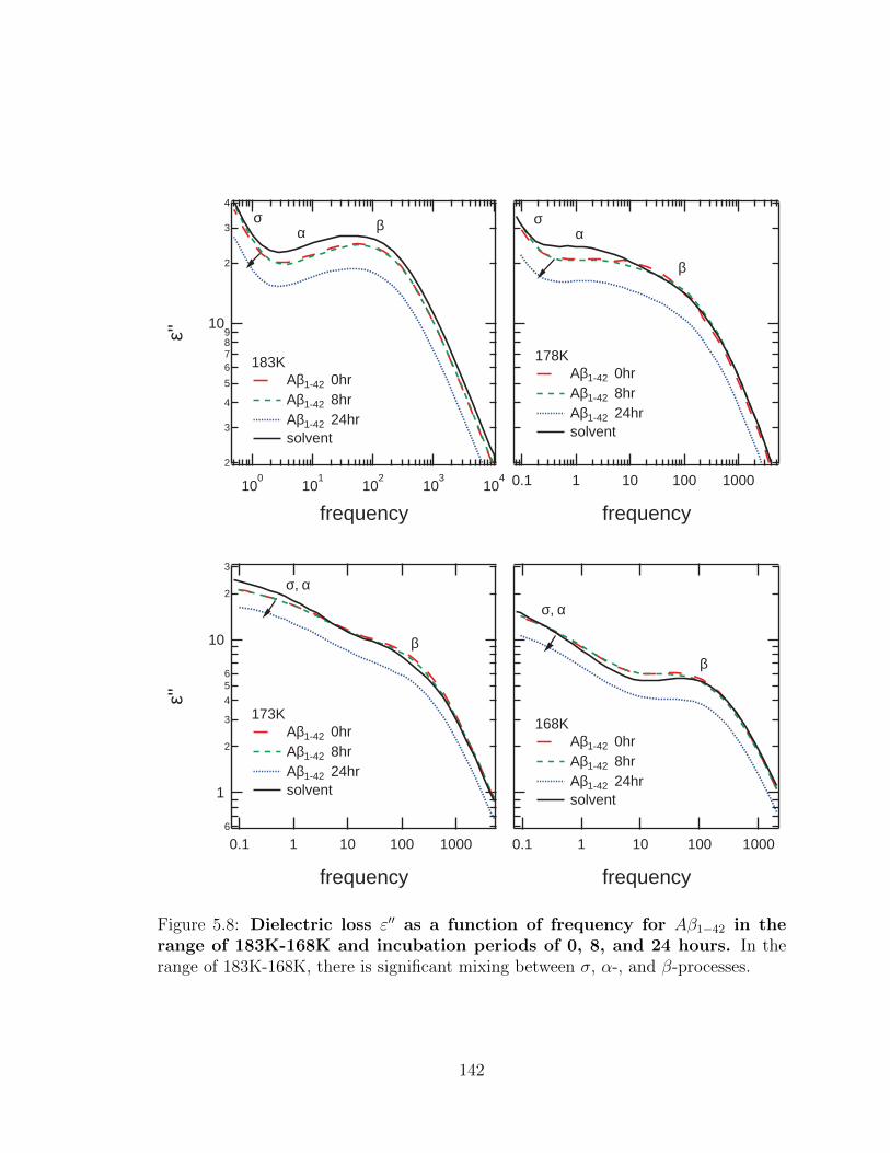
0.1 1 10 100 1000
frequency
178K Aβ1-42 0hr Aβ1-42 8hr Aβ1-42 24hr solvent
2
3
4
5
6789
10
2
3
4
ε''
100
101
102
103
104
frequency
183K Aβ1-42 0hr Aβ1-42 8hr Aβ1-42 24hr solvent
0.1 1 10 100 1000
frequency
168K Aβ1-42 0hr Aβ1-42 8hr Aβ1-42 24hr solvent
6
1
2
3
4
56
10
2
3
ε''
0.1 1 10 100 1000
frequency
173K Aβ1-42 0hr Aβ1-42 8hr Aβ1-42 24hr solvent
σα
σα
σ, α
σ, α
ββ
β
β
Figure 5.8: Dielectric loss ε′′ as a function of frequency for Aβ1−42 in therange of 183K-168K and incubation periods of 0, 8, and 24 hours. In therange of 183K-168K, there is significant mixing between σ, α-, and β-processes.
142
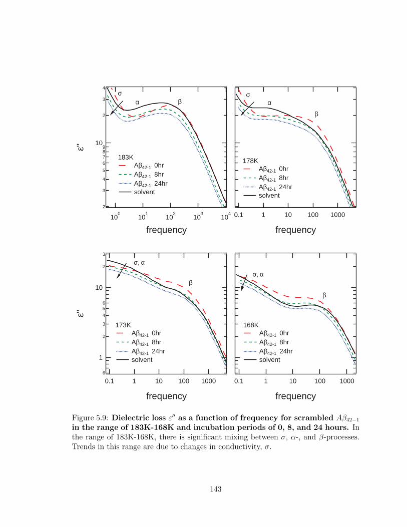
2
3
4
5
6789
10
2
3
4ε''
100
101
102
103
104
frequency
183K Aβ42-1 0hr Aβ42-1 8hr Aβ42-1 24hr solvent
0.1 1 10 100 1000
frequency
178K Aβ42-1 0hr Aβ42-1 8hr Aβ42-1 24hr solvent
0.1 1 10 100 1000
frequency
168K Aβ42-1 0hr Aβ42-1 8hr Aβ42-1 24hr solvent
6
1
2
3
4
56
10
2
3
ε''
0.1 1 10 100 1000
frequency
173K Aβ42-1 0hr Aβ42-1 8hr Aβ42-1 24hr solvent
β
β
β
β
σ σα
σ, α
σ, α
α
Figure 5.9: Dielectric loss ε′′ as a function of frequency for scrambled Aβ42−1in the range of 183K-168K and incubation periods of 0, 8, and 24 hours. Inthe range of 183K-168K, there is significant mixing between σ, α-, and β-processes.Trends in this range are due to changes in conductivity, σ.
143

5
4
3
2
1
ε''
0.1 1 10 100 1000
frequency
153K Aβ1-42 0hr Aβ1-42 8hr Aβ1-42 24hr solvent
0.1 1 10 100
frequency
148K Aβ1-42 0hr Aβ1-42 8hr Aβ1-42 24hr solvent
0.1 1 10 100 1000
frequency
158K Aβ1-42 0hr Aβ1-42 8hr Aβ1-42 24hr solvent
7
6
5
4
3
2
1
ε''
0.1 1 10 100 1000
frequency
163K Aβ1-42 0hr Aβ1-42 8hr Aβ1-42 24hr solvent
β
β
ββ
Figure 5.10: Dielectric loss ε′′ as a function of frequency for Aβ1−42 in therange of 163K-148K and incubation periods of 0, 8, and 24 hours. At 158K,the conductivity, σ and the α-process are substantially separated from the β process.At 158K and below, the β-relaxation peak in ε′′ trends to lower magnitude and lowerfrequency over time.
144
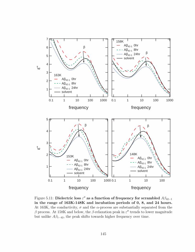
7
6
5
4
3
2
1
ε''
0.1 1 10 100 1000
frequency
163K Aβ42-1 0hr Aβ42-1 8hr Aβ42-1 24hr solvent
0.1 1 10 100 1000
frequency
158K Aβ42-1 0hr Aβ42-1 8hr Aβ42-1 24hr solvent
0.1 1 10 100
frequency
148K Aβ42-1 0hr Aβ42-1 8hr Aβ42-1 24hr solvent
5
4
3
2
1
ε''
0.1 1 10 100 1000
frequency
153K Aβ42-1 0hr Aβ42-1 8hr Aβ42-1 24hr solvent
β
β
β β
Figure 5.11: Dielectric loss ε′′ as a function of frequency for scrambled Aβ42−1in the range of 163K-148K and incubation periods of 0, 8, and 24 hours.At 163K, the conductivity, σ and the α-process are substantially separated from theβ process. At 158K and below, the β-relaxation peak in ε′′ trends to lower magnitudebut unlike Aβ1−42, the peak shifts towards higher frequency over time.
145
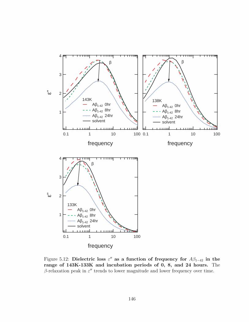
0.1 1 10 100
frequency
138K Aβ1-42 0hr Aβ1-42 8hr Aβ1-42 24hr solvent
4
3
2
1
ε''
0.1 1 10 100
frequency
143K Aβ1-42 0hr Aβ1-42 8hr Aβ1-42 24hr solvent
4
3
2
1
ε''
0.1 1 10 100
frequency
133K Aβ1-42 0hr Aβ1-42 8hr Aβ1-42 24hr solvent
β β
β
Figure 5.12: Dielectric loss ε′′ as a function of frequency for Aβ1−42 in therange of 143K-133K and incubation periods of 0, 8, and 24 hours. Theβ-relaxation peak in ε′′ trends to lower magnitude and lower frequency over time.
146

5
4
3
2
1
ε''
0.1 1 10 100
frequency
133K Aβ42-1 0hr Aβ42-1 8hr Aβ42-1 24hr solvent
0.1 1 10 100
frequency
138K Aβ42-1 0hr Aβ42-1 8hr Aβ42-1 24hr solvent
5
4
3
2
1
ε''
0.1 1 10 100
frequency
143K Aβ42-1 0hr Aβ42-1 8hr Aβ42-1 24hr solvent
β β
β
Figure 5.13: Dielectric loss ε′′ as a function of frequency for scrambled Aβ42−1in the range of 143K-133K and incubation periods of 0, 8, and 24 hours.The β-relaxation peak in ε′′ trends to lower magnitude but unlike Aβ1−42, the peakshifts towards higher frequency over time.
147
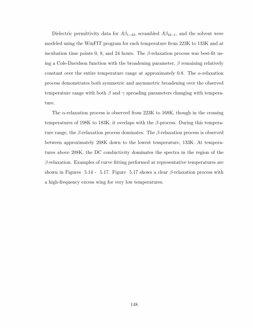
Dielectric permittivity data for Aβ1−42, scrambled Aβ42−1, and the solvent were
modeled using the WinFIT program for each temperature from 223K to 133K and at
incubation time points 0, 8, and 24 hours. The β-relaxation process was best-fit us-
ing a Cole-Davidson function with the broadening parameter, β remaining relatively
constant over the entire temperature range at approximately 0.8. The α-relaxation
process demonstrates both symmetric and asymmetric broadening over the observed
temperature range with both β and γ spreading parameters changing with tempera-
ture.
The α-relaxation process is observed from 223K to 168K, though in the crossing
temperatures of 198K to 183K, it overlaps with the β-process. During this tempera-
ture range, the β-relaxation process dominates. The β-relaxation process is observed
between approximately 208K down to the lowest temperature, 133K. At tempera-
tures above 208K, the DC conductivity dominates the spectra in the region of the
β-relaxation. Examples of curve fitting performed at representative temperatures are
shown in Figures 5.14 - 5.17. Figure 5.17 shows a clear β-relaxation process with
a high-frequency excess wing for very low temperatures.
148
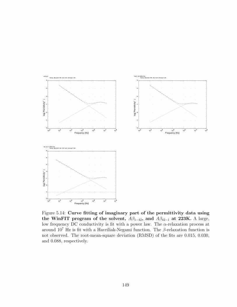
102
103
104
105
106
107
108
Frequency [Hz]
-2-1
01
23
4
log( Perm
ittivity'' )
solvent Temp. [K]=223.150 AC Volt [Vrms]=1.00
102
103
104
105
106
107
108
Frequency [Hz]
-2-1
01
23
4
log( Perm
ittivity'' )
Ab(1-42) BSA 0hr Temp. [K]=223.150 AC Volt [Vrms]=1.00
102
103
104
105
106
107
108
Frequency [Hz]
-2-1
01
23
45
log( Perm
ittivity'' )
Ab (42-1) BSA 0hr Temp. [K]=223.150 AC Volt [Vrms]=1.00
Figure 5.14: Curve fitting of imaginary part of the permittivity data usingthe WinFIT program of the solvent, Aβ1−42, and Aβ42−1 at 223K. A large,low frequency DC conductivity is fit with a power law. The α-relaxation process ataround 107 Hz is fit with a Havriliak-Negami function. The β-relaxation function isnot observed. The root-mean-square deviation (RMSD) of the fits are 0.015, 0.030,and 0.088, respectively.
149
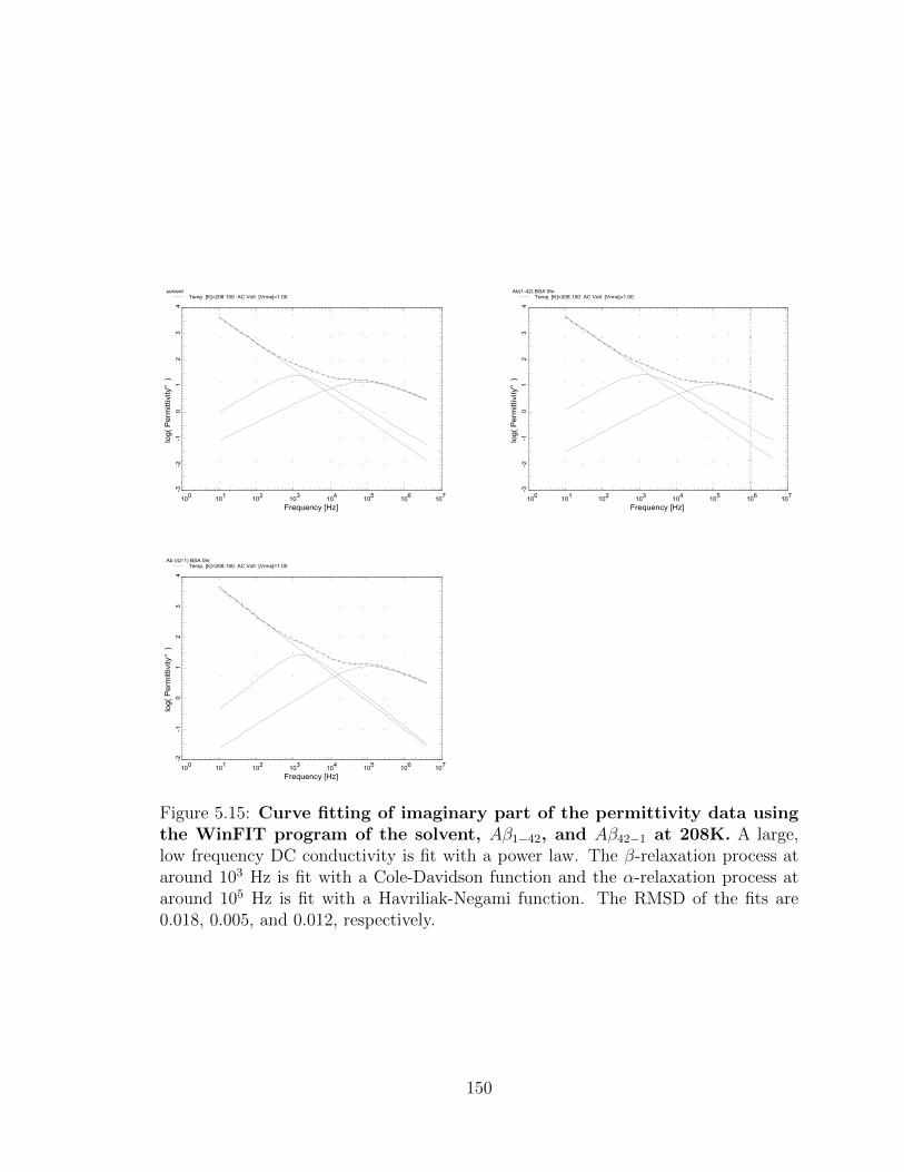
100
101
102
103
104
105
106
107
Frequency [Hz]
-3-2
-10
12
34
log
( P
erm
itti
vit
y''
)
solvent Temp. [K]=208.150 AC Volt [Vrms]=1.00
100
101
102
103
104
105
106
107
Frequency [Hz]
-3-2
-10
12
34
log
( P
erm
itti
vit
y''
)
Ab(1-42) BSA 0hr Temp. [K]=208.150 AC Volt [Vrms]=1.00
100
101
102
103
104
105
106
107
Frequency [Hz]
-2-1
01
23
4
log
( P
erm
itti
vit
y''
)
Ab (42-1) BSA 0hr Temp. [K]=208.150 AC Volt [Vrms]=1.00
Figure 5.15: Curve fitting of imaginary part of the permittivity data usingthe WinFIT program of the solvent, Aβ1−42, and Aβ42−1 at 208K. A large,low frequency DC conductivity is fit with a power law. The β-relaxation process ataround 103 Hz is fit with a Cole-Davidson function and the α-relaxation process ataround 105 Hz is fit with a Havriliak-Negami function. The RMSD of the fits are0.018, 0.005, and 0.012, respectively.
150

10-1
100
101
102
103
104
105
Frequency [Hz]
-3-2
-10
12
3
log( Perm
ittivity'' )
solvent Temp. [K]=188.150 AC Volt [Vrms]=1.00
10-1
100
101
102
103
104
105
Frequency [Hz]
-3-2
-10
12
3
log( Permittivity'' )
Ab(1-42) BSA 0 hr Temp. [K]=188.150 AC Volt [Vrms]=1.00
10-1
100
101
102
103
104
105
Frequency [Hz]
-2-1
01
23
log( Permittivity'' )
Ab(42-1) BSA 0 hr Temp. [K]=188.150 AC Volt [Vrms]=1.00
Figure 5.16: Curve fitting of imaginary part of the permittivity data usingthe WinFIT program of the solvent, Aβ1−42, and Aβ42−1 at 188K. A large,low frequency DC conductivity is fit with a power law. The β-relaxation processat around 103 Hz is fit with a Cole-Davidson function and the α-relaxation processat around 101 Hz is fit with a Havriliak-Negami function. Here, the α process hascrossed over to slower than β relaxation times. The RMSD of the fits are 0.001, 0.019,and 0.017, respectively.
151
10-2
10-1
100
101
102
103
104
Frequency [Hz]
01
23
45
Perm
ittivity''
solvent Temp. [K]=133.150 AC Volt [Vrms]=1.00
10-2
10-1
100
101
102
103
104
Frequency [Hz]0
12
34
5
Permittivity''
Ab(1-42) BSA 0 hr Temp. [K]=133.150 AC Volt [Vrms]=1.00
10-2
10-1
100
101
102
103
104
Frequency [Hz]
01
23
45
Permittivity''
Ab(42-1) BSA 0 hr Temp. [K]=133.150 AC Volt [Vrms]=1.00
Figure 5.17: Curve fitting of the imaginary part of the permittivity datausing the WinFIT program of the solvent, Aβ1−42, and Aβ42−1 at 133K. Asmall, very low frequency DC conductivity is fit with a power law. The β-relaxationprocess at around 1 Hz is fit with a Cole-Davidson function and the α-relaxationprocess is not observed. The RMSD of the fits are 0.073, 0.042, and 0.006, respectively.
152
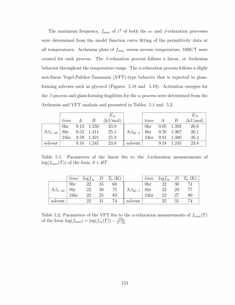
The maximum frequency, fmax of ε′′ of both the α- and β-relaxation processes
were determined from the model function curve fitting of the permittivity data at
all temperatures. Arrhenius plots of fmax versus inverse temperature, 1000/T were
created for each process. The β-relaxation process follows a linear, or Arrhenius
behavior throughout the temperature range. The α-relaxation process follows a slight
non-linear Vogel-Fulcher-Tammann (VFT)-type behavior that is expected in glass-
forming solvents such as glycerol (Figures 5.18 and 5.19). Activation energies for
the β process and glass-forming fragilities for the α process were determined from the
Arrhenius and VFT analysis and presented in Tables 5.1 and 5.2.
EA EAtime A B (kJ/mol) time A B (kJ/mol)
Aβ1−42
0hr 9.13 1.250 23.9Aβ42−1
0hr 9.95 1.392 26.68hr 9.53 1.311 25.1 8hr 9.76 1.367 26.124hr 9.59 1.321 25.3 24hr 9.91 1.380 26.4
solvent 9.18 1.245 23.8 solvent 9.18 1.245 23.8
Table 5.1: Parameters of the linear fits to the β-relaxation measurements oflog(fmax(T )) of the form A+BT .
time logf∞ D T0 (K) time logf∞ D T0 (K)
Aβ1−42
0hr 22 35 68Aβ42−1
0hr 22 30 748hr 22 30 75 8hr 22 29 7724hr 22 25 83 24hr 22 27 80
solvent 22 31 74 solvent 22 31 74
Table 5.2: Parameters of the VFT fits to the α-relaxation measurements of fmax(T )of the form log(fmax) = log(f∞(T ))− DT0
T−T0
153
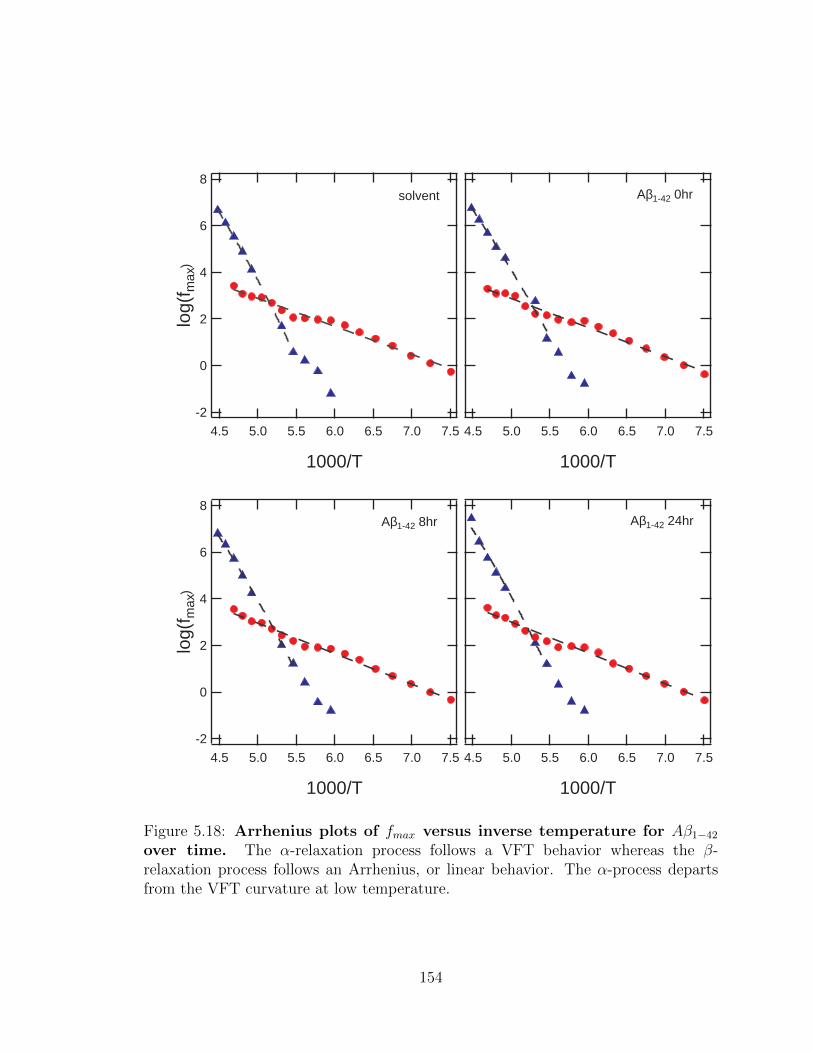
7.57.06.56.05.55.04.5
1000/T
Aβ1-42 24hr8
6
4
2
0
-2
log(
f max
)
7.57.06.56.05.55.04.5
1000/T
Aβ1-42 8hr
7.57.06.56.05.55.04.5
1000/T
Aβ1-42 0hr8
6
4
2
0
-2
log(
f max
)
7.57.06.56.05.55.04.5
1000/T
solvent
Figure 5.18: Arrhenius plots of fmax versus inverse temperature for Aβ1−42over time. The α-relaxation process follows a VFT behavior whereas the β-relaxation process follows an Arrhenius, or linear behavior. The α-process departsfrom the VFT curvature at low temperature.
154

8
6
4
2
0
-2
log(
f max
)
7.57.06.56.05.55.04.5
1000/T
solvent
7.57.06.56.05.55.04.5
1000/T
Aβ42-1 0hr
8
6
4
2
0
-2
log(
f max
)
7.57.06.56.05.55.04.5
1000/T
Aβ42-1 8hr
7.57.06.56.05.55.04.5
1000/T
Aβ42-1 24hr
Figure 5.19: Arrhenius plots of fmax versus inverse temperature for scram-bled Aβ42−1 over time. The α-relaxation process follows a VFT behavior whereasthe β-relaxation process follows an Arrhenius, or linear behavior. The α-processdeparts from the VFT curvature at low temperature.
155
The α-relaxation process for Aβ1−42, scrambled Aβ42−1, and the solvent display
VFT behavior down to 183K. Below 183K, the curvature of the VFT changes where
the temperature dependence of fmax would be better approximated by another VFT
or different empirical fit function. Studies have shown that two or more temperature-
dependent fit functions may be necessary to describe the behavior of the α-relaxation
of glass formers such as glycerol [63, 165]. The departure of the VFT behavior oc-
curs at approximately the glass transition of glycerol, indicating that the change in
temperature dependance may be due to the phase change. Whereas the α-relaxation
process is representative of large scale structural fluctuations in the solvent, it is
conceivable that a phase transition could change the temperature dependance of the
relaxation rate.
156
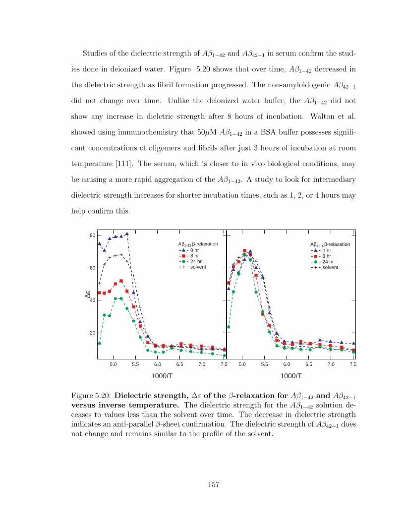
Studies of the dielectric strength of Aβ1−42 and Aβ42−1 in serum confirm the stud-
ies done in deionized water. Figure 5.20 shows that over time, Aβ1−42 decreased in
the dielectric strength as fibril formation progressed. The non-amyloidogenic Aβ42−1
did not change over time. Unlike the deionized water buffer, the Aβ1−42 did not
show any increase in dielctric strength after 8 hours of incubation. Walton et al.
showed using immunochemistry that 50µM Aβ1−42 in a BSA buffer possesses signifi-
cant concentrations of oligomers and fibrils after just 3 hours of incubation at room
temperature [111]. The serum, which is closer to in vivo biological conditions, may
be causing a more rapid aggregation of the Aβ1−42. A study to look for intermediary
dielectric strength increases for shorter incubation times, such as 1, 2, or 4 hours may
help confirm this.
80
60
40
20
∆ε
7.57.06.56.05.55.0
1000/T
Aβ1-42 β-relaxation 0 hr 8 hr 24 hr solvent
7.57.06.56.05.55.0
1000/T
Aβ42-1 β-relaxation 0 hr 8 hr 24 hr solvent
Figure 5.20: Dielectric strength, ∆ε of the β-relaxation for Aβ1−42 and Aβ42−1versus inverse temperature. The dielectric strength for the Aβ1−42 solution de-ceases to values less than the solvent over time. The decrease in dielectric strengthindicates an anti-parallel β-sheet confirmation. The dielectric strength of Aβ42−1 doesnot change and remains similar to the profile of the solvent.
157
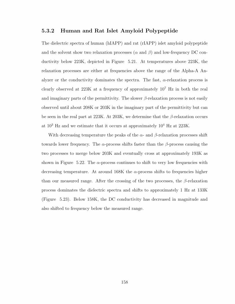
5.3.2 Human and Rat Islet Amyloid Polypeptide
The dielectric spectra of human (hIAPP) and rat (rIAPP) islet amyloid polypeptide
and the solvent show two relaxation processes (α and β) and low-frequency DC con-
ductivity below 223K, depicted in Figure 5.21. At temperatures above 223K, the
relaxation processes are either at frequencies above the range of the Alpha-A An-
alyzer or the conductivity dominates the spectra. The fast, α-relaxation process is
clearly observed at 223K at a frequency of approximately 107 Hz in both the real
and imaginary parts of the permittivity. The slower β-relaxation process is not easily
observed until about 208K or 203K in the imaginary part of the permittivity but can
be seen in the real part at 223K. At 203K, we determine that the β-relaxation occurs
at 103 Hz and we estimate that it occurs at approximately 104 Hz at 223K.
With decreasing temperature the peaks of the α- and β-relaxation processes shift
towards lower frequency. The α-process shifts faster than the β-process causing the
two processes to merge below 203K and eventually cross at approximately 193K as
shown in Figure 5.22. The α-process continues to shift to very low frequencies with
decreasing temperature. At around 168K the α-process shifts to frequencies higher
than our measured range. After the crossing of the two processes, the β-relaxation
process dominates the dielectric spectra and shifts to approximately 1 Hz at 133K
(Figure 5.23). Below 158K, the DC conductivity has decreased in magnitude and
also shifted to frequency below the measured range.
158
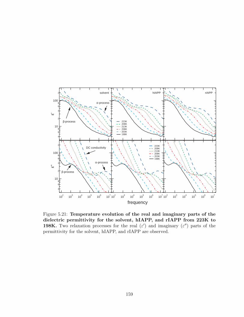
102
103
104
105
106
107
frequency
223K 208K 213K 208K 203K 198K
223K 208K 213K 208K 203K 198K
102
103
104
105
106
107
4
6
810
2
4
6
8100
2
ε'
4
6
810
2
4
6
8100
2
ε''
102
103
104
105
106
107
solvent hIAPP rIAPP
α-process
α-process
β-process
β-process
DC conductivity
Figure 5.21: Temperature evolution of the real and imaginary parts of thedielectric permittivity for the solvent, hIAPP, and rIAPP from 223K to198K. Two relaxation processes for the real (ε′) and imaginary (ε′′) parts of thepermittivity for the solvent, hIAPP, and rIAPP are observed.
159
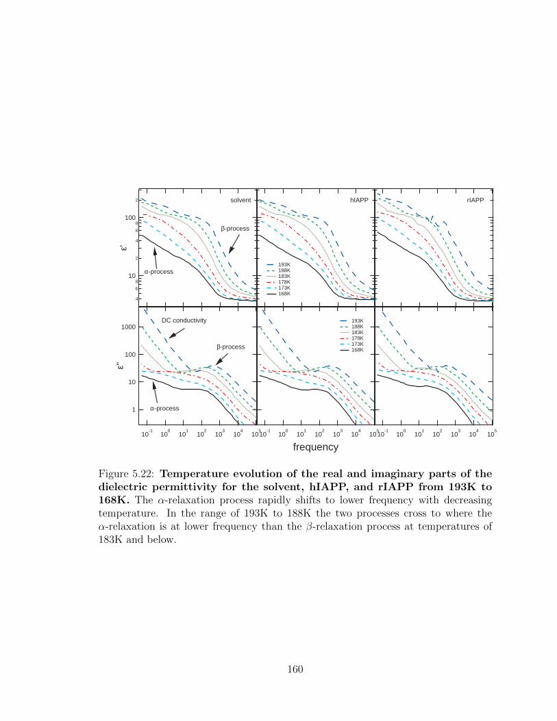
10-1
100
101
102
103
104
105
frequency
193K 188K 183K 178K 173K 168K
193K 188K 183K 178K 173K 168K
4
6
810
2
4
6
8100
2
ε'
10-1
100
101
102
103
104
105
1
10
100
1000
ε''
10-1
100
101
102
103
104
105
solvent hIAPP rIAPP
β-process
β-process
α-process
α-process
DC conductivity
Figure 5.22: Temperature evolution of the real and imaginary parts of thedielectric permittivity for the solvent, hIAPP, and rIAPP from 193K to168K. The α-relaxation process rapidly shifts to lower frequency with decreasingtemperature. In the range of 193K to 188K the two processes cross to where theα-relaxation is at lower frequency than the β-relaxation process at temperatures of183K and below.
160
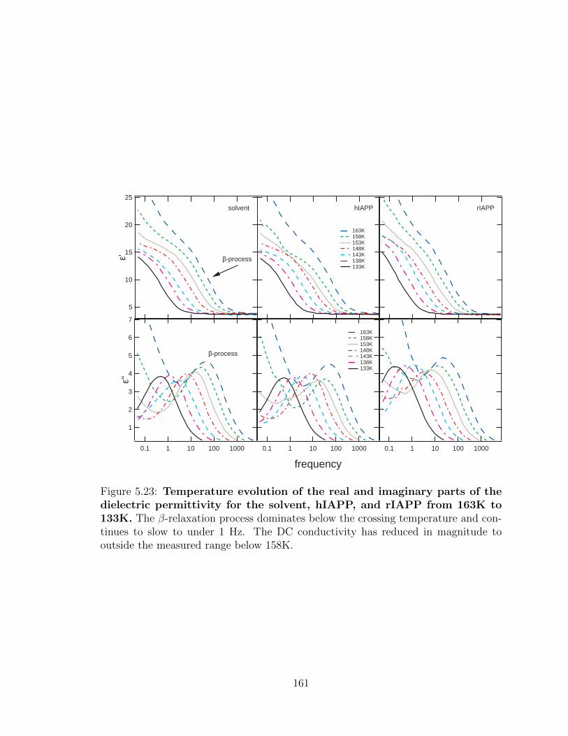
0.1 1 10 100 1000
frequency
163K 158K 153K 148K 143K 138K 133K
163K 158K 153K 148K 143K 138K 133K
7
6
5
4
3
2
1
ε''
0.1 1 10 100 1000
25
20
15
10
5
ε'
0.1 1 10 100 1000
solvent hIAPP rIAPP
β-process
β-process
Figure 5.23: Temperature evolution of the real and imaginary parts of thedielectric permittivity for the solvent, hIAPP, and rIAPP from 163K to133K. The β-relaxation process dominates below the crossing temperature and con-tinues to slow to under 1 Hz. The DC conductivity has reduced in magnitude tooutside the measured range below 158K.
161
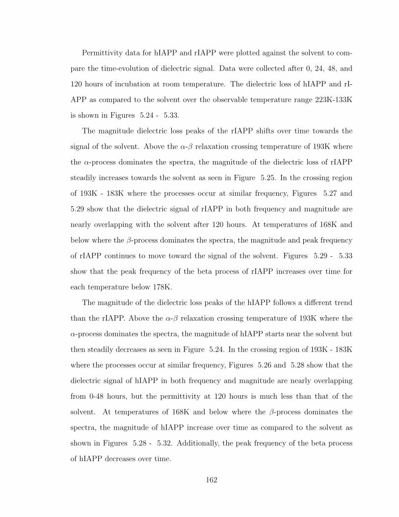
Permittivity data for hIAPP and rIAPP were plotted against the solvent to com-
pare the time-evolution of dielectric signal. Data were collected after 0, 24, 48, and
120 hours of incubation at room temperature. The dielectric loss of hIAPP and rI-
APP as compared to the solvent over the observable temperature range 223K-133K
is shown in Figures 5.24 - 5.33.
The magnitude dielectric loss peaks of the rIAPP shifts over time towards the
signal of the solvent. Above the α-β relaxation crossing temperature of 193K where
the α-process dominates the spectra, the magnitude of the dielectric loss of rIAPP
steadily increases towards the solvent as seen in Figure 5.25. In the crossing region
of 193K - 183K where the processes occur at similar frequency, Figures 5.27 and
5.29 show that the dielectric signal of rIAPP in both frequency and magnitude are
nearly overlapping with the solvent after 120 hours. At temperatures of 168K and
below where the β-process dominates the spectra, the magnitude and peak frequency
of rIAPP continues to move toward the signal of the solvent. Figures 5.29 - 5.33
show that the peak frequency of the beta process of rIAPP increases over time for
each temperature below 178K.
The magnitude of the dielectric loss peaks of the hIAPP follows a different trend
than the rIAPP. Above the α-β relaxation crossing temperature of 193K where the
α-process dominates the spectra, the magnitude of hIAPP starts near the solvent but
then steadily decreases as seen in Figure 5.24. In the crossing region of 193K - 183K
where the processes occur at similar frequency, Figures 5.26 and 5.28 show that the
dielectric signal of hIAPP in both frequency and magnitude are nearly overlapping
from 0-48 hours, but the permittivity at 120 hours is much less than that of the
solvent. At temperatures of 168K and below where the β-process dominates the
spectra, the magnitude of hIAPP increase over time as compared to the solvent as
shown in Figures 5.28 - 5.32. Additionally, the peak frequency of the beta process
of hIAPP decreases over time.
162
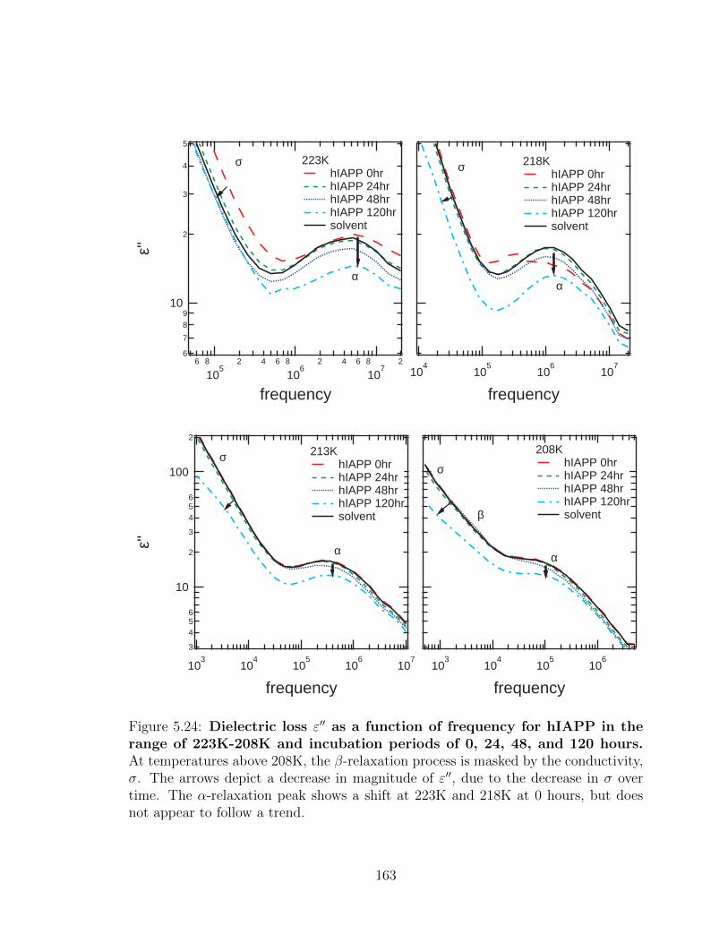
104
105
106
107
frequency
218K hIAPP 0hr hIAPP 24hr hIAPP 48hr hIAPP 120hr solvent
103
104
105
106
frequency
208K hIAPP 0hr hIAPP 24hr hIAPP 48hr hIAPP 120hr solvent
3
456
10
2
3
456
100
2
ε''
103
104
105
106
107
frequency
213K hIAPP 0hr hIAPP 24hr hIAPP 48hr hIAPP 120hr solvent
6
7
89
10
2
3
4
5ε''
6 8
105
2 4 6 8
106
2 4 6 8
107
2
frequency
223K hIAPP 0hr hIAPP 24hr hIAPP 48hr hIAPP 120hr solvent
σ σ
σσ
αα
α α
β
Figure 5.24: Dielectric loss ε′′ as a function of frequency for hIAPP in therange of 223K-208K and incubation periods of 0, 24, 48, and 120 hours.At temperatures above 208K, the β-relaxation process is masked by the conductivity,σ. The arrows depict a decrease in magnitude of ε′′, due to the decrease in σ overtime. The α-relaxation peak shows a shift at 223K and 218K at 0 hours, but doesnot appear to follow a trend.
163

3
456
10
2
3
456
100
2
ε''
103
104
105
106
107
frequency
213K rIAPP 0hr rIAPP 24hr rIAPP 48hr rIAPP 120hr solvent
6 8
103
2 4 6 8
104
2 4 6 8
105
2 4
frequency
208K rIAPP 0hr rIAPP 24hr rIAPP 48hr rIAPP 120hr solvent
104
105
106
107
frequency
218K rIAPP 0hr rIAPP 24hr rIAPP 48hr rIAPP 120hr solvent
6
7
89
10
2
3
4
5ε''
6 8
105
2 4 6 8
106
2 4 6 8
107
2
frequency
223K rIAPP 0hr rIAPP 24hr rIAPP 48hr rIAPP 120hr solvent
σ σ
σ σ
α α
α α
β
Figure 5.25: Dielectric loss ε′′ as a function of frequency for rIAPP in therange of 223K-208K and incubation periods of 0, 24, 48, and 120 hours.At temperatures above 208K, the β-relaxation process is masked by the conductivity,σ. The arrows depict an apparent shift in the α-relaxation process first to lower mag-nitude and frequency, then higher magnitude and frequency. This differs in behaviorto hIAPP in the same temperature range.
164
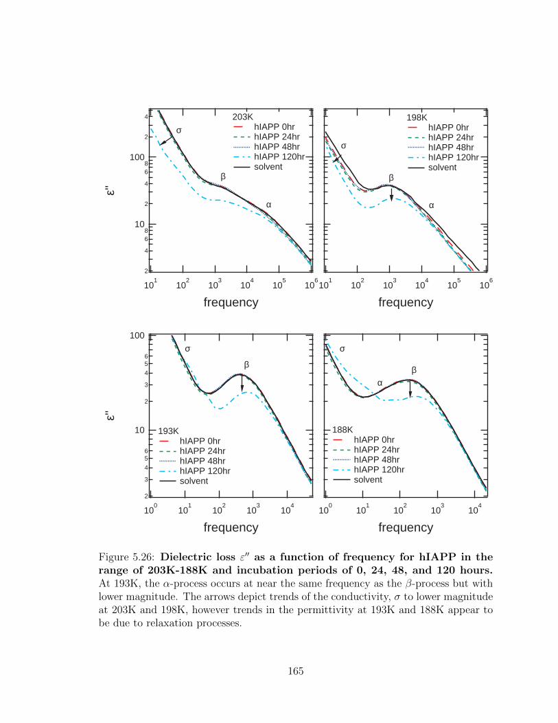
2
4
68
10
2
4
68
100
2
4ε''
101
102
103
104
105
106
frequency
203K hIAPP 0hr hIAPP 24hr hIAPP 48hr hIAPP 120hr solvent
101
102
103
104
105
106
frequency
198K hIAPP 0hr hIAPP 24hr hIAPP 48hr hIAPP 120hr solvent
100
101
102
103
104
frequency
188K hIAPP 0hr hIAPP 24hr hIAPP 48hr hIAPP 120hr solvent
2
3
4
56
10
2
3
4
56
100
ε''
100
101
102
103
104
frequency
193K hIAPP 0hr hIAPP 24hr hIAPP 48hr hIAPP 120hr solvent
σ
σ
σ σ
β β
β βα
αα
Figure 5.26: Dielectric loss ε′′ as a function of frequency for hIAPP in therange of 203K-188K and incubation periods of 0, 24, 48, and 120 hours.At 193K, the α-process occurs at near the same frequency as the β-process but withlower magnitude. The arrows depict trends of the conductivity, σ to lower magnitudeat 203K and 198K, however trends in the permittivity at 193K and 188K appear tobe due to relaxation processes.
165
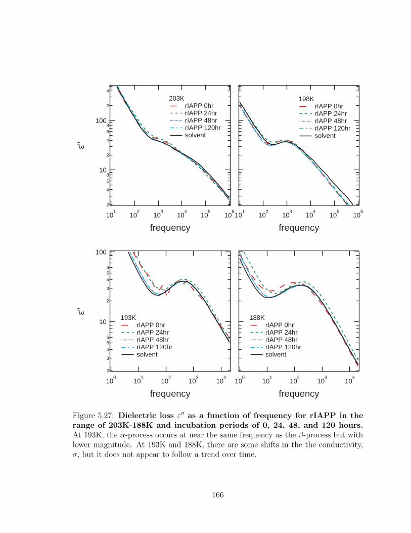
101
102
103
104
105
106
frequency
198K rIAPP 0hr rIAPP 24hr rIAPP 48hr rIAPP 120hr solvent
100
101
102
103
104
frequency
188K rIAPP 0hr rIAPP 24hr rIAPP 48hr rIAPP 120hr solvent
2
3
4
56
10
2
3
4
56
100
ε''
100
101
102
103
104
frequency
193K rIAPP 0hr rIAPP 24hr rIAPP 48hr rIAPP 120hr solvent
2
4
68
10
2
4
68
100
2
4
ε''
101
102
103
104
105
106
frequency
203K rIAPP 0hr rIAPP 24hr rIAPP 48hr rIAPP 120hr solvent
Figure 5.27: Dielectric loss ε′′ as a function of frequency for rIAPP in therange of 203K-188K and incubation periods of 0, 24, 48, and 120 hours.At 193K, the α-process occurs at near the same frequency as the β-process but withlower magnitude. At 193K and 188K, there are some shifts in the the conductivity,σ, but it does not appear to follow a trend over time.
166
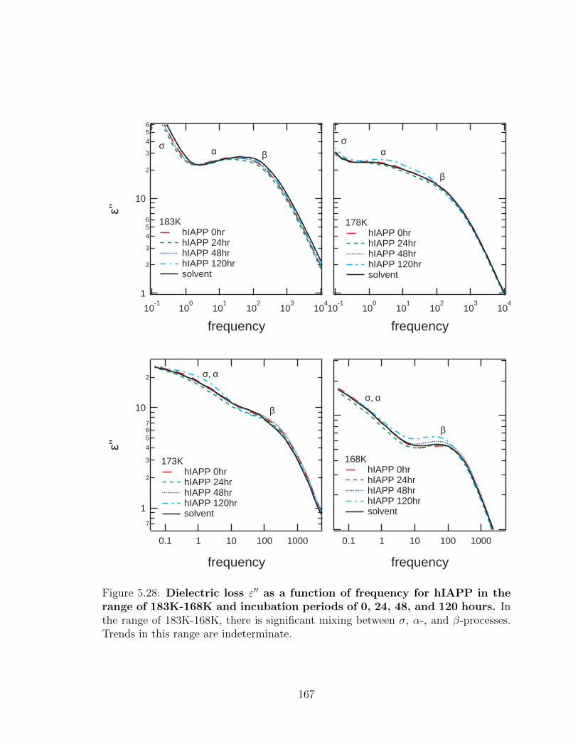
7
1
2
3
4
567
10
2
ε''
0.1 1 10 100 1000
frequency
173K hIAPP 0hr hIAPP 24hr hIAPP 48hr hIAPP 120hr solvent
0.1 1 10 100 1000
frequency
168K hIAPP 0hr hIAPP 24hr hIAPP 48hr hIAPP 120hr solvent
10-1
100
101
102
103
104
frequency
178K hIAPP 0hr hIAPP 24hr hIAPP 48hr hIAPP 120hr solvent
1
2
3
456
10
2
3
456
ε''
10-1
100
101
102
103
104
frequency
183K hIAPP 0hr hIAPP 24hr hIAPP 48hr hIAPP 120hr solvent
σ α α
σ, α
σ, αβ
β
β
βσ
Figure 5.28: Dielectric loss ε′′ as a function of frequency for hIAPP in therange of 183K-168K and incubation periods of 0, 24, 48, and 120 hours. Inthe range of 183K-168K, there is significant mixing between σ, α-, and β-processes.Trends in this range are indeterminate.
167
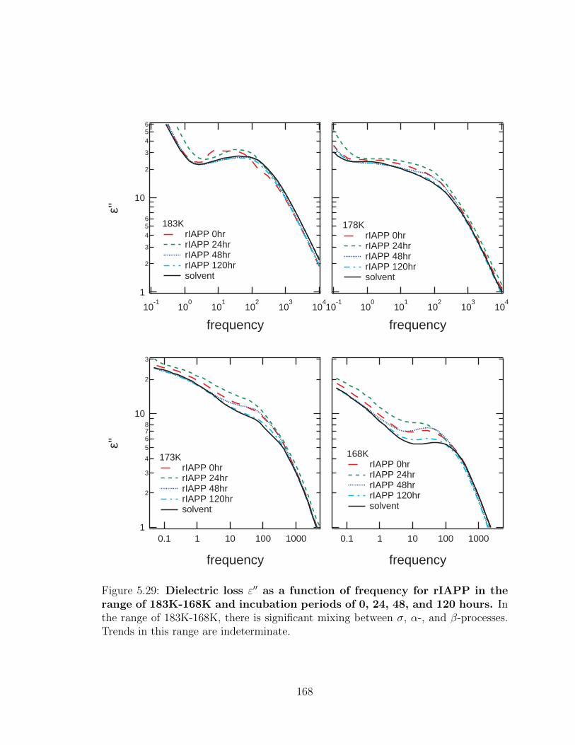
1
2
3
4
5678
10
2
3
ε''
0.1 1 10 100 1000
frequency
173K rIAPP 0hr rIAPP 24hr rIAPP 48hr rIAPP 120hr solvent
0.1 1 10 100 1000
frequency
168K rIAPP 0hr rIAPP 24hr rIAPP 48hr rIAPP 120hr solvent
10-1
100
101
102
103
104
frequency
178K rIAPP 0hr rIAPP 24hr rIAPP 48hr rIAPP 120hr solvent
1
2
3
456
10
2
3
456
ε''
10-1
100
101
102
103
104
frequency
183K rIAPP 0hr rIAPP 24hr rIAPP 48hr rIAPP 120hr solvent
Figure 5.29: Dielectric loss ε′′ as a function of frequency for rIAPP in therange of 183K-168K and incubation periods of 0, 24, 48, and 120 hours. Inthe range of 183K-168K, there is significant mixing between σ, α-, and β-processes.Trends in this range are indeterminate.
168

8
6
4
2
ε''
1 10 100 1000
frequency
163K hIAPP 0hr hIAPP 24hr hIAPP 48hr hIAPP 120hr solvent
0.1 1 10 100 1000
frequency
158K hIAPP 0hr hIAPP 24hr hIAPP 48hr hIAPP 120hr solvent
5
4
3
2
1
0
ε''
0.1 1 10 100 1000
frequency
153K hIAPP 0hr hIAPP 24hr hIAPP 48hr hIAPP 120hr solvent
0.1 1 10 100 1000
frequency
148K hIAPP 0hr hIAPP 24hr hIAPP 48hr hIAPP 120hr solvent
ββ
β β
σ, α
Figure 5.30: Dielectric loss ε′′ as a function of frequency for hIAPP in therange of 163K-148K and incubation periods of 0, 24, 48, and 120 hours. At158K, the conductivity, σ and the α-process are substantially separated from the βprocess. At 158K and below, the β-relaxation peak in ε′′ trends to higher magnitudeand lower frequency over time.
169
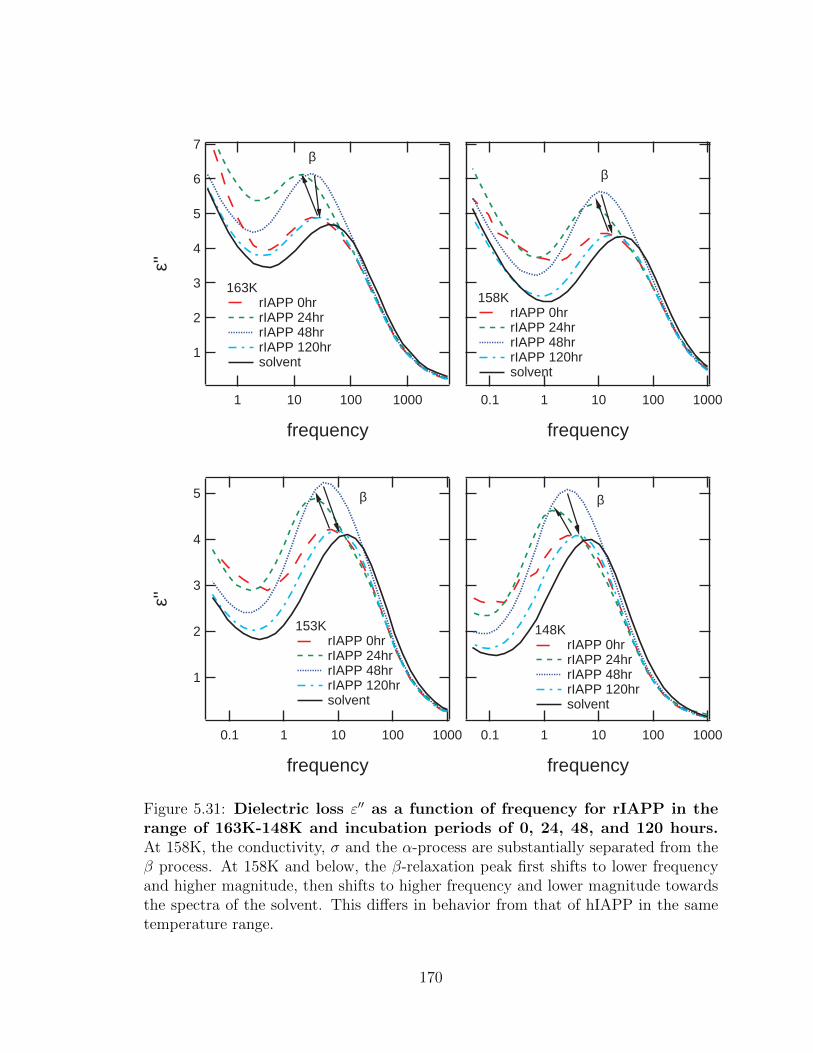
0.1 1 10 100 1000
frequency
148K rIAPP 0hr rIAPP 24hr rIAPP 48hr rIAPP 120hr solvent
5
4
3
2
1
ε''
0.1 1 10 100 1000
frequency
153K rIAPP 0hr rIAPP 24hr rIAPP 48hr rIAPP 120hr solvent
0.1 1 10 100 1000
frequency
158K rIAPP 0hr rIAPP 24hr rIAPP 48hr rIAPP 120hr solvent
7
6
5
4
3
2
1
ε''
1 10 100 1000
frequency
163K rIAPP 0hr rIAPP 24hr rIAPP 48hr rIAPP 120hr solvent
ββ
β β
Figure 5.31: Dielectric loss ε′′ as a function of frequency for rIAPP in therange of 163K-148K and incubation periods of 0, 24, 48, and 120 hours.At 158K, the conductivity, σ and the α-process are substantially separated from theβ process. At 158K and below, the β-relaxation peak first shifts to lower frequencyand higher magnitude, then shifts to higher frequency and lower magnitude towardsthe spectra of the solvent. This differs in behavior from that of hIAPP in the sametemperature range.
170
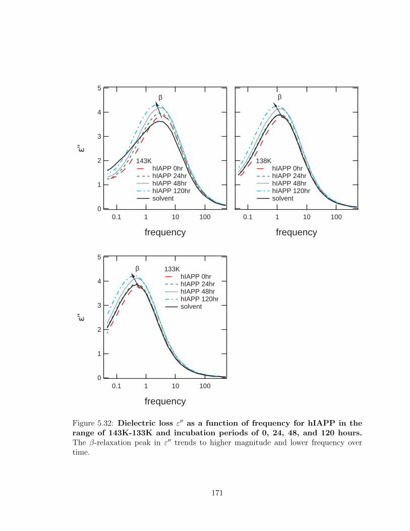
5
4
3
2
1
0
ε''
0.1 1 10 100
frequency
143K hIAPP 0hr hIAPP 24hr hIAPP 48hr hIAPP 120hr solvent
0.1 1 10 100
frequency
138K hIAPP 0hr hIAPP 24hr hIAPP 48hr hIAPP 120hr solvent
5
4
3
2
1
0
ε''
0.1 1 10 100
frequency
133K hIAPP 0hr hIAPP 24hr hIAPP 48hr hIAPP 120hr solvent
β β
β
Figure 5.32: Dielectric loss ε′′ as a function of frequency for hIAPP in therange of 143K-133K and incubation periods of 0, 24, 48, and 120 hours.The β-relaxation peak in ε′′ trends to higher magnitude and lower frequency overtime.
171
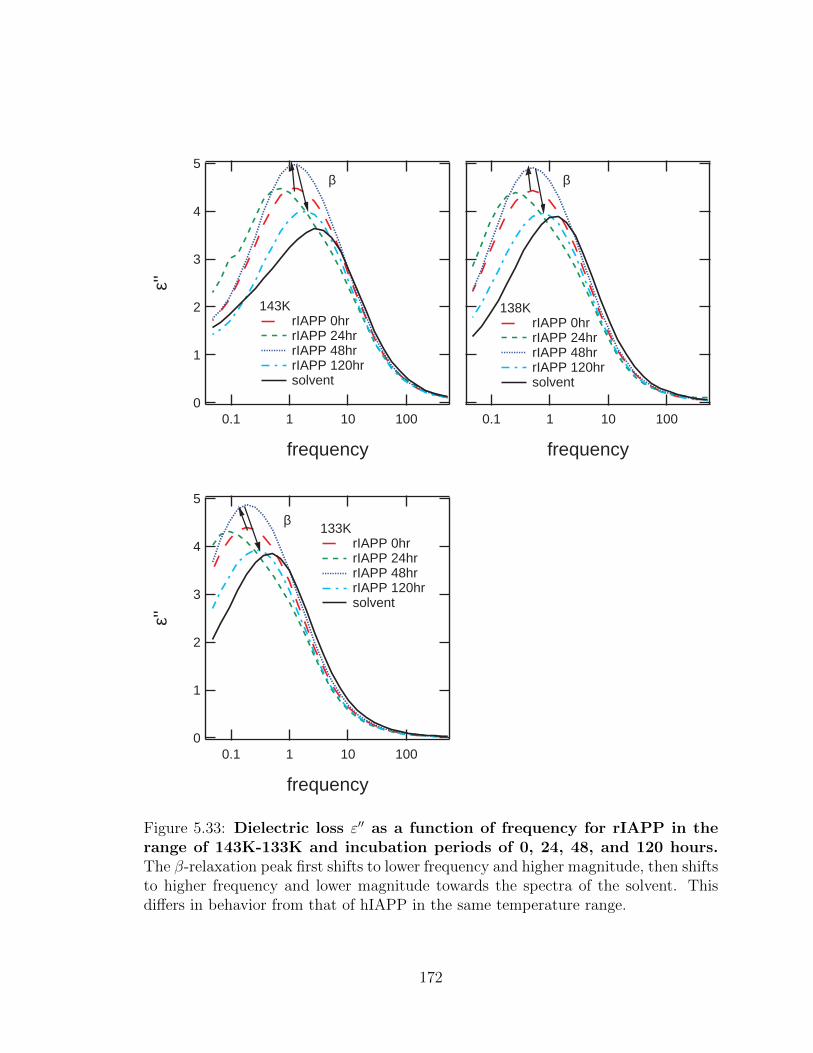
0.1 1 10 100
frequency
138K rIAPP 0hr rIAPP 24hr rIAPP 48hr rIAPP 120hr solvent
5
4
3
2
1
0
ε''
0.1 1 10 100
frequency
143K rIAPP 0hr rIAPP 24hr rIAPP 48hr rIAPP 120hr solvent
5
4
3
2
1
0
ε''
0.1 1 10 100
frequency
133K rIAPP 0hr rIAPP 24hr rIAPP 48hr rIAPP 120hr solvent
β β
β
Figure 5.33: Dielectric loss ε′′ as a function of frequency for rIAPP in therange of 143K-133K and incubation periods of 0, 24, 48, and 120 hours.The β-relaxation peak first shifts to lower frequency and higher magnitude, then shiftsto higher frequency and lower magnitude towards the spectra of the solvent. Thisdiffers in behavior from that of hIAPP in the same temperature range.
172
Dielectric permittivity data for hIAPP, rIAPP, and the solvent were modeled us-
ing the WinFIT program for each temperature from 223K to 133K and at incubation
time points 0, 24, 48, and 120 hours. The β-relaxation process is best-fit to a Cole-
Davidson with the symmetric broadening parameter, β remaining relatively constant
over the entire temperature range at approximately 0.8. The α-relaxation process
demonstrates both symmetric and asymmetric broadening over the observed temper-
ature range with both β and γ spreading parameters changing with temperature.
The α-relaxation process is observed from 223K to 168K, though in the crossing
temperatures of 198K to 183K, it overlaps with the β-process. During this tempera-
ture range, the β-relaxation process dominates. The β-relaxation process is observed
between approximately 208K down to the lowest temperature, 133K. At tempera-
tures above 208K, the DC conductivity dominates the spectra in the region of the
β-relaxation. Examples of curve fitting performed at representative temperatures are
shown in Figures 5.34 - 5.37.
173

102
103
104
105
106
107
108
Frequency [Hz]
-2-1
01
23
4
log( Perm
ittivity'' )
solvent Temp. [K]=223.150 AC Volt [Vrms]=1.00
102
103
104
105
106
107
108
Frequency [Hz]-2
-10
12
34
5
log( Perm
ittivity'' )
HIAPP_BSA_0HR Temp. [K]=223.150 AC Volt [Vrms]=1.00
101
102
103
104
105
106
107
108
Frequency [Hz]
-4-2
02
46
log( Perm
ittivity'' )
RIAPP_BSA_0HR Temp. [K]=223.150 AC Volt [Vrms]=1.00
Figure 5.34: Curve fitting of imaginary part of the permittivity data usingthe WinFIT program of the solvent, hIAPP, and rIAPP at 223K. A large,low frequency DC conductivity is fit with a power law. The α-relaxation process ataround 107 Hz is fit with a Havriliak-Negami function. The β-relaxation function isnot observed. The RMSD of the fits are 0.015, 0.016, and 0.034, respectively.
174

100
101
102
103
104
105
106
107
Frequency [Hz]
-3-2
-10
12
34
log
( P
erm
itti
vit
y''
)
solvent Temp. [K]=208.150 AC Volt [Vrms]=1.00
100
101
102
103
104
105
106
107
Frequency [Hz]
-2-1
01
23
4
log
( P
erm
itti
vit
y''
)
HIAPP_BSA_0HR Temp. [K]=208.150 AC Volt [Vrms]=1.00
100
101
102
103
104
105
106
107
Frequency [Hz]
-4-2
02
46
log
( P
erm
itti
vit
y''
)
RIAPP_BSA_0HR Temp. [K]=208.150 AC Volt [Vrms]=1.00
Figure 5.35: Curve fitting of imaginary part of the permittivity data usingthe WinFIT program of the solvent, hIAPP, and rIAPP at 208K. A large,low frequency DC conductivity is fit with a power law. The β-relaxation process ataround 103 Hz is fit with a Cole-Davidson function and the α-relaxation process ataround 105 Hz is fit with a Havriliak-Negami function. The RMSD of the fits are0.018, 0.007, and 0.020, respectively.
175
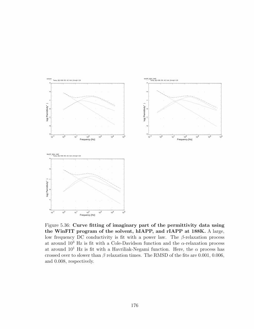
10-1
100
101
102
103
104
105
Frequency [Hz]
-3-2
-10
12
3
log( Perm
ittivity'' )
solvent Temp. [K]=188.150 AC Volt [Vrms]=1.00
10-1
100
101
102
103
104
105
Frequency [Hz]
-3-2
-10
12
3
log(
Perm
ittivity''
)
HIAPP_BSA_0HR Temp. [K]=188.150 AC Volt [Vrms]=1.00
10-1
100
101
102
103
104
105
Frequency [Hz]
-2-1
01
23
log( Permittivity'' )
RIAPP_BSA_0HR Temp. [K]=188.150 AC Volt [Vrms]=1.00
Figure 5.36: Curve fitting of imaginary part of the permittivity data usingthe WinFIT program of the solvent, hIAPP, and rIAPP at 188K. A large,low frequency DC conductivity is fit with a power law. The β-relaxation processat around 103 Hz is fit with a Cole-Davidson function and the α-relaxation processat around 101 Hz is fit with a Havriliak-Negami function. Here, the α process hascrossed over to slower than β relaxation times. The RMSD of the fits are 0.001, 0.006,and 0.008, respectively.
176

10-2
10-1
100
101
102
103
104
Frequency [Hz]
01
23
45
Perm
ittivity''
solvent Temp. [K]=133.150 AC Volt [Vrms]=1.00
10-2
10-1
100
101
102
103
104
Frequency [Hz]0
12
34
5
Permittivity''
HIAPP_BSA_0HR Temp. [K]=133.150 AC Volt [Vrms]=1.00
10-2
10-1
100
101
102
103
104
Frequency [Hz]
01
23
45
Permittivity''
RIAPP_BSA_0HR Temp. [K]=133.150 AC Volt [Vrms]=1.00
Figure 5.37: Curve fitting of the imaginary part of the permittivity datausing the WinFIT program of the solvent, hIAPP, rIAPP at 133K. A small,very low frequency DC conductivity is fit with a power law. The β-relaxation processat around 1 Hz is fit with a Cole-Davidson function and the α-relaxation process isnot observed. The RMSD of the fits are 0.073, 0.090, and 0.035, respectively.
177
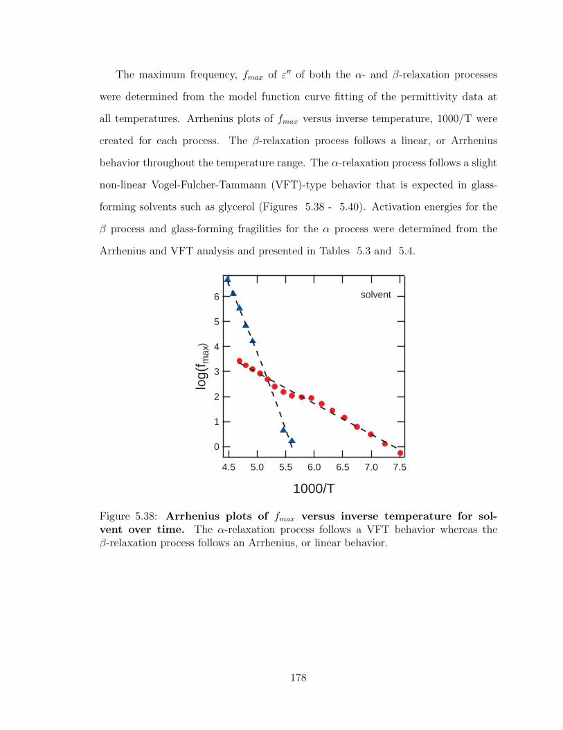
The maximum frequency, fmax of ε′′ of both the α- and β-relaxation processes
were determined from the model function curve fitting of the permittivity data at
all temperatures. Arrhenius plots of fmax versus inverse temperature, 1000/T were
created for each process. The β-relaxation process follows a linear, or Arrhenius
behavior throughout the temperature range. The α-relaxation process follows a slight
non-linear Vogel-Fulcher-Tammann (VFT)-type behavior that is expected in glass-
forming solvents such as glycerol (Figures 5.38 - 5.40). Activation energies for the
β process and glass-forming fragilities for the α process were determined from the
Arrhenius and VFT analysis and presented in Tables 5.3 and 5.4.
6
5
4
3
2
1
0
log(
f max
)
7.57.06.56.05.55.04.5
1000/T
solvent
Figure 5.38: Arrhenius plots of fmax versus inverse temperature for sol-vent over time. The α-relaxation process follows a VFT behavior whereas theβ-relaxation process follows an Arrhenius, or linear behavior.
178
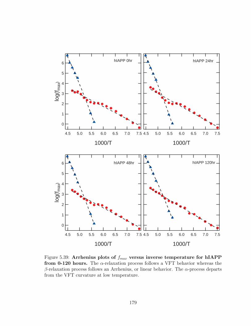
7.57.06.56.05.55.04.5
1000/T
hIAPP 120hr
6
5
4
3
2
1
0
log(
f max
)
7.57.06.56.05.55.04.5
1000/T
hIAPP 0hr
6
5
4
3
2
1
0
log(
f max
)
7.57.06.56.05.55.04.5
1000/T
hIAPP 48hr
7.57.06.56.05.55.04.5
1000/T
hIAPP 24hr
Figure 5.39: Arrhenius plots of fmax versus inverse temperature for hIAPPfrom 0-120 hours. The α-relaxation process follows a VFT behavior whereas theβ-relaxation process follows an Arrhenius, or linear behavior. The α-process departsfrom the VFT curvature at low temperature.
179

7.57.06.56.05.55.04.5
1000/T
rIAPP 120hr
7.57.06.56.05.55.04.5
1000/T
rIAPP 24hr6
5
4
3
2
1
0
log(
f max
)
7.57.06.56.05.55.04.5
1000/T
rIAPP 0hr
6
5
4
3
2
1
0
log(
f max
)
7.57.06.56.05.55.04.5
1000/T
rIAPP 48hr
Figure 5.40: Arrhenius plots of fmax versus inverse temperature for rIAPPfrom 0-120 hours. The α-relaxation process follows a VFT behavior whereas theβ-relaxation process follows an Arrhenius, or linear behavior. The α-process departsfrom the VFT curvature at low temperature.
180

EA EAtime A B (kJ/mol) time A B (kJ/mol)
hIAPP
0hr 9.02 1.216 23.3
rIAPP
0hr 10.0 1.412 27.024hr 9.44 1.289 24.7 24hr 10.6 1.540 29.548hr 9.10 1.237 23.7 48hr 10.5 1.494 28.6120hr 9.97 1.373 26.3 120hr 9.70 1.338 25.6
solvent 9.18 1.245 23.8 solvent 9.18 1.245 23.8
Table 5.3: Parameters of the linear fits to the β-relaxation measurements oflog(fmax(T )) of the form A+BT .
time logf∞ D T0 (K) time logf∞ D T0 (K)
hIAPP
0hr 22 32 72
rIAPP
0hr 22 40 6324hr 22 32 73 24hr 22 44 5948hr 22 33 71 48hr 22 36 67120hr 22 40 62 120hr 22 35 69
solvent 22 31 74 solvent 22 31 74
Table 5.4: Parameters of the VFT fits to the α-relaxation measurements of fmax(T )of the form log(fmax) = log(f∞(T ))− DT0
T−T0
181
The α-relaxation process for hIAPP, rIAPP, and the solvent display VFT behavior
down to 183K. Below 183K, the curvature of the VFT changes where the tempera-
ture dependance of fmax would be better approximated by another VFT or different
empirical fit function. Studies have shown that two or more temperature-dependent
fit functions may be necessary to describe the behavior of the α-relaxation of glass
formers such as glycerol [63, 165]. The departure of the VFT behavior occurs at
approximately the glass transition of glycerol, indicating that the change in tempera-
ture dependance may be due to the phase change. Whereas the α-relaxation process
is representative of large scale structural fluctuations in the solvent, it is conceivable
that a phase transition could change the temperature dependance of the relaxation
rate.
Studies of the dielectric strength of hIAPP and rIAPP in serum confirm the stud-
ies done in deionized water. Figure 5.41 shows that over time, hIAPP displayed
a series of increases and decreases in the dielectric strength as fibril formation pro-
gresses, with a final dielectric strength much less than the solvent at 120 hours. The
non-amyloidogenic rIAPP did not change over time. The increase and decrease cy-
cles for hIAPP may be due to a mixture of both parallel and anti-parallel β-sheet
conformations dominating at different phases of the aggregation process, but here we
see a final state that would appear to be anti-parallel in nature.
182

80
60
40
20
∆ε
7.57.06.56.05.55.0
1000/T
hIAPP β-relaxation 0 hr 24 hr 48 hr 120 hr solvent
7.57.06.56.05.55.0
1000/T
rIAPP β-relaxation 0 hr 24 hr 48 hr 120 hr solvent
Figure 5.41: Dielectric strength, ∆ε of the β-relaxation for hIAPP and rI-APP versus inverse temperature. The dielectric strength for the hIAPP solutionremains relatively constant for the first 48 hours, then deceases to values less than thesolvent after 120 hours of incubation. This may be an indication that the final ag-gregated state of hIAPP in serum is an anti-parallel β-sheet. The dielectric strengthof rIAPP was similar to the solvent for all time points. This is a similar ∆ε behaviorof Aβ1−42 and Aβ42− 1 observed for the same solvent.
183
5.4 Conclusions
We have demonstrated the dielectric response of Aβ1−42, scrambled Aβ42−1, hIAPP,
and rIAPP in the presence of a BSA-glycerol solvent. The spectra reveal that
these amyloidogenic peptides can be detected and differentiated from their non-
amyloidogenic analogs in the presence of other proteins and biological substances,
similar to in vivo conditions. This is a crucial step in demonstrating the viability of
using dielectric relaxation spectroscopy as a tool for detecting amyloidogenic peptides
in biological fluids, such as blood serum.
Studies at low temperature reveal that the β-process displays a characteristic
”red-shift” in the permittivity in both Aβ1−42 and hIAPP that is not observed in
Aβ42−1 and rIAPP (see Figure 5.42). Theory predicts that this red-shift occurs due
to a hinderance of the rotational motion of molecular dipoles in structured, biological
water [64, 166]. This restructuring of the hydrogen bond network as a result of
hydrophobic interactions causes a reduction in the hydrogen bond exchange. We also
observed the red-shift in the hIAPP measurements in deionized water (see Figure
4.42) but not previously in Aβ1−42.
Studies of the dielectric strength over a range of temperatures and incubation
times show that determination of β-sheet conformation by dielectric spectroscopy is
in agreement with previous studies done using FTIR and solid state NMR. The Aβ1−42
displayed anti-parallel characteristics and the hIAPP displayed both parallel and anti-
parallel signatures. The non-amyloidogenic peptides produced dipole moments that
would be consistent with random coil or non-aggregating proteins.
The change in dielectric strength of the peptides in serum is a further extension
to the information presented in deionized water buffer. Both Aβ1−42 and hIAPP
displayed a decrease in the dielectric strength from start to final time points. The
Aβ1−42 displayed a larger decrease and in shorter time, indicating that Aβ1−42 may
form oligomers and fibrils faster than hIAPP. The lack of changing dielectric strength
184

2x100
3
4
5
ε''
0.12 3 4 5 6 7
12 3 4 5 6 7
102
frequency
Aβ1-42 0hr Aβ1-42 24hr Aβ42-1 0hr Aβ42-1 24hr solvent
2x100
3
4
5
ε''
4 5 60.1
2 3 4 5 61
2 3 4 5 610
2
frequency
hIAPP 0hr hIAPP 120hr rIAPP 0hr rIAPP 120hr solvent
Figure 5.42: Plots of the β-relaxation peak shift at 143K for Aβ1−42/Aβ42−1and hIAPP/rIAPP as compared to the solvent. The amyloidogenic peptidesdemonstrate a characteristic ”red- shift” towards tower frequencies, indicating anincrease in structured water.
for both non-amyloidogenic peptides Aβ42−1 and rIAPP was expected for a random
aggregation of protein lacking a β-sheet.
185

Chapter 6
Conclusion
6.1 General Conclusions
At present, there is no unequivocal method for the early detection for amyloid-related
diseases such as Alzheimer’s and Type II Diabetes. Although it was long believed that
amyloidogenic diseases were caused by highly organized fibrillar aggregates, recent
theory and experiment has shown that the soluble oligomer forms of these peptides
are the most toxic form. Amyloid oligomers circulate freely through bodily fluids
[18, 17, 16] and thus, detection of soluble amyloid aggregates might represent the best
strategy for early detection. Although there have been several attempts to develop
diagnostic methods based on the detection of amyloidogenic oligomers, there is an
absence of a widely-accepted and deterministic approach.
The work presented in this thesis has focussed on the studies of amyloidogenic
peptides using dielectric relaxation spectroscopy (DRS). Dielectric measurements per-
formed over a broadband of frequencies (10−2-107), temperature ranges from 133K-
300K, and incubation times up to 7 days has revealed patterns that may be used to
classify these peptides in various media.
186

Amyloidogenic peptides amyloid beta (Aβ1−42) and human islet amyloid polypep-
tide (hIAPP) were used as analytes in these studies, with their non-amyloidogenic
analogs, scrambled Aβ42−1 and rat islet amyloid polypeptide (rIAPP) as controls.
These amyloidogenic peptides are known to aggregate into well-ordered fibrillar struc-
tures, namely the β-sheet conformation. Our hypothesis is that structural changes
during the fibrillization process causes a re-ordering of water molecules due to the
hydrophobicity of exposed amino acids. This re-ordering of water can be observed in
the protein-solvent relaxations using DRS.
Studies of the peptides at room temperature revealed that there is a large contribu-
tion to the conductivity and space-charge polarization due to the heterogeneity of the
peptide-solvent mixture. The dielectric modulus formalism was used to reveal changes
in the conductivity relaxation peaks between amyloidogenic and non-amyloidogenic
peptides over time.
The dielectric response of the peptides in a deionized water-glycerol solvent re-
vealed that amyloidogenic peptides in their in purified (non-in vivo-like) form can
be detected and differentiated from their non-amyloidogenic analogs. Studies at low
temperature revealed that the β-process displayed a decrease in the dielectric loss,
ε′′ for both amyloidogenic Aβ1−42 and hIAPP and an increase for non-amyloidogenic
Aβ42−1 and rIAPP. This may point to an increase in fraction of structured water over
time associated with the amyloidogenic peptides during β-sheet formation. The trend
observed in the non-amyloidogenic peptides reflects that a random aggregation lacks
the large fraction of structured water that is contained in a organized β-sheet.
The dielectric response of the peptides in the presence of a BSA-glycerol solvent
revealed that these amyloidogenic peptides can be detected and differentiated from
their non-amyloidogenic analogs in the presence of other proteins and biological sub-
stances, similar to in vivo conditions. This is a crucial step in demonstrating the
viability of using dielectric relaxation spectroscopy as a tool for detecting amyloido-
187

genic peptides in biological fluids, such as blood serum. Studies at low temperature
revealed that the β-process displays a characteristic ”red-shift” in the permittivity in
both Aβ1−42 and hIAPP that is not observed in Aβ42−1 and rIAPP (see Figure 5.42).
Theory predicts that this red-shift occurs due to a hinderance of the rotational mo-
tion of molecular dipoles in structured, biological water [64, 166]. This restructuring
of the hydrogen bond network as a result of hydrophobic interactions causes a reduc-
tion in the hydrogen bond exchange. We also observed the red-shift in the hIAPP
measurements in deionized water (see Figure 4.42) but not previously in Aβ1−42.
Analysis of the dielectric strength showed that the macroscopic dipole moment of
the amyloidogenic protein-solvent solutions changed over time in a different manner
than the non-amyloidogenic peptides. The decreasing dipole moment upon fibril
formation of Aβ1−42 in both deionized water and serum buffers confirms the results
found by FTIR and solid state NMR that the structure is comprised of anti-parallel
β-sheets. The intermediate increase in dipole moment of Aβ1−42 in DI buffer may be
indicative of a high fraction of oligomers. Oligomers of Aβ1−42 form a reverse micelle
that should display a net increase in the dipole moment. The collective dipole moment
of Aβ1−42 at different incubation times could be used to determine the domination
aggregate species, whether monomer, oligomer, or fibril forms. The varying dipole
moment of hIAPP over time may be due to a mixture of both parallel and anti-
parallel sheets, as published in the literature from FTIR and NMR studies. The
non-amyloidogenic peptides either increased in collective dipole moment or did not
change at all. This would indicate that if any aggregation occurred, it may be α-helix
or random coil.
We note that the limits of sensitivity of DRS as a tool to study amyloidogenic
peptides has not yet been tested. Serum concentration of β-amyloid in Alzheimer’s
patients has been found on the order of 100 nM (nanomolar) [167] and concentrations
of IAPP in Type II Diabetes has been found on the order of 10pM (picomolar) [168].
188
Future work to determine the detectable limit of amyloidogenic peptides using DRS
is an important examination.
Recent theory suggests that protein motions are slaved to solvent fluctuations
[58, 59]. Studies of solvent relaxation processes yield insight into protein fluctuations,
structure, and function. Measurements of the time evolution and relaxation kinetics
of α- and β-relaxation processes allow us to model dielectric permittivity to the
various phases of fibril formation. We demonstrated that amyloidogenic peptides,
in general, move towards lower activation energy, confirming that the fibrillar state
is thermodynamically favorable and stable. The observation that the amyloidogenic
peptides displayed a lower activation energy as compared to their non-amyloidogenic
analogs would indicate a higher fraction of structured water in the amyloid β-sheet.
6.2 Future Direction
This work demonstrates that studies of the time evolution of dielectric permittivity by
use of dielectric relaxation spectroscopy can reveal differences between amyloidogenic
peptides and their non-amyloidogenic analogs. The following is an outline a suggested
plan for further work to develop a method for using DRS as a tool for detecting toxic
pre-amyloid aggregates in patient samples.
6.2.1 Expansion of DRS Methods
Measurements we have performed thus far have only begun to explore the dielec-
tric properties of amyloidogenic peptides. Thermal studies to examine the dielectric
response during heating, as well as cooling would show if there are reversible pro-
cesses and any hysteresis effects. Additionally, thermal quenching techniques can be
implored to rapidly freeze the system to study particular phases. Other input pa-
rameters, such as the driving AC electric field, V0 for the DRS measurements can
189
be varied to study a dependency on the strength of the field. A study of the dielec-
tric response as a function of the applied electric field could give further insight into
deformation polarization effects.
6.2.2 Miniaturized sample cell
Broadband dielectric relaxation spectroscopy is an important tool to study molecular
dynamics in broad temperature and frequency ranges. It has the additional advan-
tage that the sensitivity of the measurement increases with decrease sample thickness
[169]. Using nano-scale components, information about single molecules and molecu-
lar assemblies is an attainable goal [170]. For example, Kremer et al. used 10nm gap
sizes to probe the molecular dynamics of polymers and suggest this method as a tool
for studying nano-biophysics [169]. A continuation of this work using a sample cell
with micrometer or nanometer gap size may lead to additional information about the
dielectric behavior of amyloidogenic peptides by exploring their microscopic behavior.
6.2.3 Amyloid fibril inhibitors
Since detection of soluble, pre-fibrillar amyloid structures is the end-goal for a diag-
nostic test, there is a desire to definitively correlate the dielectric signal with various
stages of oligomerization and fibril growth. Several small molecules have been identi-
fied that inhibit the formation of amyloid fibrils from monomers [171, 172, 173, 174].
These inhibitors can be used in vitro to stop the aggregation process at the different
phases of fibril formation. From this, one can classify dielectric spectra with each
particular phase. Further insight into fibril formation rates and possibly quantitative
measurements of pre-amyloid oligomers may be possible by using these inhibitors.
190
6.2.4 Complementary analysis tools
A number of measurement and analysis tools have been used in the study of amy-
loidogenic peptides and their aggregates (see Section 1.6). Electron microscopy (EM)
and atomic force microscopy (AFM) are possible choices for confirmatory tools to cor-
relate dielectric spectra with phases of fibril formation. EM can be used to show the
presence of pre-fibrillar oligomers at various concentrations, incubation times, and
buffers. Both EM and AFM can be used to image the size and shape of amyloid
fibrils to verify the end-point of fibril formation.
6.2.5 Serum studies
The studies we have performed thus far have been on purified peptides placed in a
solution of deionized water or bovine serum albumin (BSA). A continuation of this
work would be to obtain serum samples from transgenic mice models that are known
to have various stages of clinical Type II diabetes and Alzheimer’s disease. Use of the
pathogenic murine models and known controls can be used to correlate a quantitative
measurement of pre-amyloid oligomers in blood-serum media. A further continuation
would be to perform the same experiments using human serum of clinical and non-
clinical donors.
191
Bibliography
[1] Life expectancy. http://en.wikipedia.org/wiki/Life_expectancy. Ac-cessed: 09/03/2013.
[2] Liesi E. Hebert, Jennifer Weuve, Paul A. Scherr, and Denis A. Evans. Alzheimerdisease in the United States (2010–2050) estimated using the 2010 census. Neu-rology, 2013.
[3] Alzhiemer’s association. http://www.alz.org. Accessed: 24/09/2012.
[4] Alzheimer’s Association. 2012 alzheimer’s disease facts and figures. Alzheimer’sand dementia the journal of the Alzheimer’s Association, 6(2):131–168, 2012.
[5] American diabetes association. http://www.diabetes.org. Accessed:24/09/2012.
[6] Center for Disease Control and Prevention. 2011 national diabetes fact sheet.2011.
[7] Claudio Soto. Protein misfolding and disease; protein refolding and therapy.FEBS Letters, 498(2-3):204 – 207, 2001. ¡ce:title¿Lisbon Special Issue¡/ce:title¿.
[8] Christopher M. Dobson. The structural basis of protein folding and its linkswith human disease. Philosophical Transactions of the Royal Society of London.Series B: Biological Sciences, 356(1406):133–145, 2001.
[9] Christopher M. Dobson. Protein misfolding, evolution and disease. Trends inBiochemical Sciences, 24(9):329 – 332, 1999.
[10] George G. Glenner and Caine W. Wong. Alzheimer’s disease: Initial report ofthe purification and characterization of a novel cerebrovascular amyloid protein.Biochemical and Biophysical Research Communications, 120(3):885 – 890, 1984.
[11] Dennis J. Selkoe. Alzheimer’s disease genes, proteins, and therapy. PhysiologicalReviews, 81(2):741–766, 2001.
[12] Magdalena Anguiano, Richard J. Nowak, and Peter T. Lansbury. Protofibrillarislet amyloid polypeptide permeabilizes synthetic vesicles by a pore-like mech-anism that may be relevant to type ii diabetes. Biochemistry, 41(38):11338–11343, 2002. PMID: 12234175.
192

[13] Byron Caughey and Peter T. Lansbury. Protofibrils, pores, fibrils, and neurode-generation: Separating the responsible protein aggregates from the innocentbystanders*. Annual Review of Neuroscience, 26(1):267–298, 2003.
[14] Marina D. Kirkitadze, Gal Bitan, and David B. Teplow. Paradigm shifts inalzheimer’s disease and other neurodegenerative disorders: The emerging role ofoligomeric assemblies. Journal of Neuroscience Research, 69(5):567–577, 2002.
[15] Kelly A. Conway, Seung-Jae Lee, Jean-Christophe Rochet, Tomas T. Ding,Robin E. Williamson, and Peter T. Lansbury. Acceleration of oligomerization,not fibrillization, is a shared property of both a-synuclein mutations linkedto early-onset parkinson’s disease: Implications for pathogenesis and therapy.Proceedings of the National Academy of Sciences, 97(2):571–576, 2000.
[16] Rakez Kayed, Elizabeth Head, Jennifer L. Thompson, Theresa M. McIntire,Saskia C. Milton, Carl W. Cotman, and Charles G. Glabe. Common structure ofsoluble amyloid oligomers implies common mechanism of pathogenesis. Science,300(5618):486–489, 2003.
[17] Alex E. Roher, Jerome Baudry, Michael O. Chaney, Yu-Min Kuo, W.BlaineStine, and Mark R. Emmerling. Oligomerization and fibril assembly of theamyloid-beta protein. Biochimica et Biophysica Acta (BBA) - Molecular Basisof Disease, 1502(1):31 – 43, 2000.
[18] Dennis J. Selkoe. Physiological production of the beta-amyloid protein and themechanism of alzheimer’s disease. Trends in Neurosciences, 16(10):403 – 409,1993.
[19] Rainulf A. Stelzmann, H. Norman Schnitzlein, and F. Reed Murtagh. An en-glish translation of alzheimer’s 1907 paper, uber eine eigenartige erkankung derhirnrinde. Clinical Anatomy, 8(6):429–431, 1995.
[20] Dominic M. Walsh, Aleksey Lomakin, George B. Benedek, Margaret M. Con-dron, and David B. Teplow. Amyloid beta-protein fibrillogenesis. Journal ofBiological Chemistry, 272(35):22364–22372, 1997.
[21] S. S. Mirra, A. Heyman, D. McKeel, S. M. Sumi, B. J. Crain, L. M. Brownlee,F. S. Vogel, J. P. Hughes, G. van Belle, and L. Berg. The consortium to establisha registry for alzheimer’s disease. Neurology, 41(4):479, 1991.
[22] John Hardy and David Allsop. Amyloid deposition as the central event in theaetiology of alzheimer’s disease. Trends in Pharmacological Sciences, 12(0):383–388, 1991.
[23] Lars O. Tjernberg, Jan Naslund, Fredrik Lindqvist, Jan Johansson, Anders R.Karlstrom, Johan Thyberg, Lars Terenius, and Christer Nordstedt. Arrest ofbeta-amyloid fibril formation by a pentapeptide ligand. Journal of BiologicalChemistry, 271(15):8545–8548, 1996.
193
[24] Salim S. El-Amouri, Hong Zhu, Jin Yu, Robert Marr, Inder M. Verma, andMark S. Kindy. Neprilysin: An enzyme candidate to slow the progression ofalzheimer’s disease. The American Journal of Pathology, 172(5):1342–1354,2008.
[25] BA Yankner, LK Duffy, and DA Kirschner. Neurotrophic and neurotoxic ef-fects of amyloid beta protein: reversal by tachykinin neuropeptides. Science,250(4978):279–282, 1990.
[26] N Arispe, E Rojas, and H B Pollard. Alzheimer disease amyloid beta proteinforms calcium channels in bilayer membranes: blockade by tromethamine andaluminum. Proceedings of the National Academy of Sciences, 90(2):567–571,1993.
[27] Masahiro Kawahara and Yoichiro Kuroda. Molecular mechanism of neurode-generation induced by alzheimer’s beta-amyloid protein: channel formation anddisruption of calcium homeostasis. Brain Research Bulletin, 53(4):389–397,2000.
[28] Jorge Ghiso, Miguel Calero, Etsuro Matsubara, Samuel Governale, JosephChuba, Ronald Beavis, Thomas Wisniewski, and Blas Frangione. Alzheimer’ssoluble amyloid beta is a normal component of human urine. FEBS Letters,408(1):105–108, 1997.
[29] P Westermark, C Wernstedt, E Wilander, D W Hayden, T D O’Brien, and K HJohnson. Amyloid fibrils in human insulinoma and islets of langerhans of thediabetic cat are derived from a neuropeptide-like protein also present in normalislet cells. Proceedings of the National Academy of Sciences, 84(11):3881–3885,1987.
[30] A. Lorenzo and B. A. Yankner. Amyloid fibril toxicity in alzheimer’s diseaseand diabetesa. Annals of the New York Academy of Sciences, 777(1):89–95,1996.
[31] P Westermark, U Engstrom, K H Johnson, G T Westermark, and C Betsholtz.Islet amyloid polypeptide: pinpointing amino acid residues linked to amyloidfibril formation. Proceedings of the National Academy of Sciences, 87(13):5036–5040, 1990.
[32] Christer Betsholtz, Lars Christmansson, Ulla Engstram, Frederik Rorsman,Viveka Svensson, Kenneth H. Johnson, and Per Westermark. Sequence diver-gence in a specific region of islet amyloid polypeptide (iapp) explains differencesin islet amyloid formation between species. FEBS Letters, 251(1-2):261 – 264,1989.
[33] M Nishi, S J Chan, S Nagamatsu, G I Bell, and D F Steiner. Conservation ofthe sequence of islet amyloid polypeptide in five mammals is consistent with
194
its putative role as an islet hormone. Proceedings of the National Academy ofSciences, 86(15):5738–5742, 1989.
[34] Tajib A. Mirzabekov, Meng-chin Lin, and Bruce L. Kagan. Pore formation bythe cytotoxic islet amyloid peptide amylin. Journal of Biological Chemistry,271(4):1988–1992, 1996.
[35] Steven E. Kahn. The importance of beta-cell failure in the development andprogression of type 2 diabetes. Journal of Clinical Endocrinology & Metabolism,86(9):4047–4058, 2001.
[36] E. Hartter, T. Svoboda, B. Ludvik, M. Schuller, B. Lell, E. Kuenburg,M. Brunnbauer, W. Woloszczuk, and R. Prager. Basal and stimulated plasmalevels of pancreatic amylin indicate its co-secretion with insulin in humans.Diabetologia, 34:52–54, 1991. 10.1007/BF00404025.
[37] J.M. Berg, J.L. Tymoczko, and L. Stryer. Biochemistry. W. H. Freeman, 2006.
[38] R.H. Garrett and C.M. Grisham. Biochemistry. Thomson Brooks/Cole, 1999.
[39] I.N. Serdyuk, N.R. Zaccai, and J. Zaccai. Methods in Molecular Biophysics:Structure, Dynamics, Function. Cambridge University Press, 2007.
[40] Aphrodite Kapurniotu. Amyloidogenicity and cytotoxicity of islet amyloidpolypeptide. Peptide Science, 60(6):438–459, 2001.
[41] Mihael H. Polymeropoulos, Christian Lavedan, Elisabeth Leroy, Susan E.Ide, Anindya Dehejia, Amalia Dutra, Brian Pike, Holly Root, Jeffrey Ruben-stein, Rebecca Boyer, Edward S. Stenroos, Settara Chandrasekharappa, AglaiaAthanassiadou, Theodore Papapetropoulos, William G. Johnson, Alice M. Laz-zarini, Roger C. Duvoisin, Giuseppe Di Iorio, Lawrence I. Golbe, and Robert L.Nussbaum. Mutation in the alpha-synuclein gene identified in families withparkinson’s disease. Science, 276(5321):2045–2047, 1997.
[42] Yoshio Namba, Masanori Tomonaga, Hiroshi Kawasaki, Eiichi Otomo, andKazuhiko Ikeda. Apolipoprotein e immunoreactivity in cerebral amyloid de-posits and neurofibrillary tangles in alzheimer’s disease and kuru plaque amyloidin creutzfeldt-jakob disease. Brain Research, 541(1):163 – 166, 1991.
[43] Richard T. Johnson and Clarence J. Gibbs. Creutzfeldt-jakob disease andrelated transmissible spongiform encephalopathies. New England Journal ofMedicine, 339(27):1994–2004, 1998.
[44] C. Soto. Alzheimer’s and prion disease as disorders of protein conformation: im-plications for the design of novel therapeutic approaches. Journal of MolecularMedicine, 77:412–418, 1999. 10.1007/s001090050371.
195

[45] C. Soto. Alzheimer’s and prion disease as disorders of protein conformation: im-plications for the design of novel therapeutic approaches. Journal of MolecularMedicine, 77:412–418, 1999. 10.1007/s001090050371.
[46] Ehud Gazit. The ”correctly folded” state of proteins: Is it a metastable state?Angewandte Chemie International Edition, 41(2):257–259, 2002.
[47] Fabrizio Chiti and Christopher M. Dobson. Protein misfolding, functional amy-loid, and human disease. Annual Review of Biochemistry, 75(1):333–366, 2006.
[48] Stanley B Prusiner, Michael R Scott, Stephen J DeArmond, and Fred E Cohen.Prion protein biology. Cell, 93(3):337 – 348, 1998.
[49] Fabrizio Chiti, Paul Webster, Niccola Taddei, Anne Clark, Massimo Stefani,Giampietro Ramponi, and Christopher M. Dobson. Designing conditions forin vitro formation of amyloid protofilaments and fibrils. Proceedings of theNational Academy of Sciences, 96(7):3590–3594, 1999.
[50] Rainer Jaenicke and Robert Seckler. Protein misassembly in vitro. In DavidS. Eisenberg Frederic M. Richards and Peter S. Kim, editors, Protein Misas-sembly, volume 50 of Advances in Protein Chemistry, pages 1 – C10. AcademicPress, 1997.
[51] D A Kirschner, C Abraham, and D J Selkoe. X-ray diffraction from intra-neuronal paired helical filaments and extraneuronal amyloid fibers in alzheimerdisease indicates cross-beta conformation. Proceedings of the National Academyof Sciences, 83(2):503–507, 1986.
[52] Charles G. Glabe. Structural classification of toxic amyloid oligomers. Journalof Biological Chemistry, 283(44):29639–29643, 2008.
[53] Fabrizio Chiti, Niccolo Taddei, Fabiana Baroni, Cristina Capanni, MassimoStefani, Giampietro Ramponi, and Christopher M. Dobson. Kinetic partitioningof protein folding and aggregation. Nature Structural Biology, 9(2):137–143,2003.
[54] Kazuhiro Hasegawa, Itaru Yamaguchi, Saburou Omata, Fumitake Gejyo, andHironobu Naiki. Interaction between abeta(1-42) and abeta(1-40) in alzheimer’sbeta-amyloid fibril formation in vitro. Biochemistry, 38(47):15514–15521, 1999.
[55] Rebecca Nelson, Michael R. Sawaya, Melinda Balbirnie, Anders O. Madsen,Christian Riekel, Robert Grothe, and David Eisenberg. Structure of the cross-beta spine of amyloid-like fibrils. Nature, 435(7043):773–778, 2005.
[56] Aneta T. Petkova, Yoshitaka Ishii, John J. Balbach, Oleg N. Antzutkin,Richard D. Leapman, Frank Delaglio, and Robert Tycko. A structural modelfor alzheimer’s beta-amyloid fibrils based on experimental constraints from solidstate nmr. Proceedings of the National Academy of Sciences, 99(26):16742–16747, 2002.
196
[57] P. W. Fenimore, H. Frauenfelder, B. H. McMahon, and F. G. Parak. Slaving:Solvent fluctuations dominate protein dynamics and functions. Proceedings ofthe National Academy of Sciences, 99(25):16047–16051, 2002.
[58] H. Frauenfelder, P. W. Fenimore, G. Chen, and B. H. McMahon. Protein foldingis slaved to solvent motions. Proceedings of the National Academy of Sciences,103(42):15469–15472, 2006.
[59] Hans Frauenfelder, Guo Chen, Joel Berendzen, Paul W. Fenimore, Helen Jans-son, Benjamin H. McMahon, Izabela R. Stroe, Jan Swenson, and Robert D.Young. A unified model of protein dynamics. Proceedings of the NationalAcademy of Sciences, pages 1–6, 2009.
[60] P. W. Fenimore, Hans Frauenfelder, B. H. McMahon, and R. D. Young. Bulk-solvent and hydration-shell fluctuations, similar to alpha- and beta-fluctuationsin glasses, control protein motions and functions. Proceedings of the NationalAcademy of Sciences, 101(40):14408–14413, 2004.
[61] Vassiliy Lubchenko, Peter G. Wolynes, and Hans Frauenfelder. Mosaic energylandscapes of liquids and the control of protein conformational dynamics byglass-forming solvents. The Journal of Physical Chemistry B, 109(15):7488–7499, 2005.
[62] G. Chen, P.W. Fenimore, H. Frauenfelder, F. Mezei, J. Swenson, and R.D.Young. Protein fluctuations explored by inelastic neutron scattering and di-electric relaxation spectroscopy. Philosophical Magazine, 88(33-35):3877–3883,2008.
[63] F. Kremer and A. Schonhals. Broadband Dielectric Spectroscopy. Springer,2003.
[64] Florin Despa. Biological water. Annals of the New York Academy of Sciences,1066(1):1–11, 2006.
[65] Orlando Crescenzi, Simona Tomaselli, Remo Guerrini, Severo Salvadori,Anna M. D’Ursi, Piero Andrea Temussi, and Delia Picone. Solution structureof the alzheimer amyloid beta-peptide (1-42) in an apolar microenvironment.European Journal of Biochemistry, 269(22):5642–5648, 2002.
[66] T.M. Nordlund. Quantitative Understanding of Biosystems: An Introductionto Biophysics. Taylor & Francis, 2010.
[67] G D Rose and R Wolfenden. Hydrogen bonding, hydrophobicity, packing,and protein folding. Annual Review of Biophysics and Biomolecular Structure,22(1):381–415, 1993.
[68] F M Richards. Areas, volumes, packing, and protein structure. Annual Reviewof Biophysics and Bioengineering, 6(1):151–176, 1977.
197
[69] G Otting, E Liepinsh, and K Wuthrich. Protein hydration in aqueous solution.Science, 254(5034):974–980, 1991.
[70] J. L. Oncley. Studies of the dielectric properties of protein solutions. i. carboxy-hemoglobin1,2. Journal of the American Chemical Society, 60(5):1115–1123,1938.
[71] J. L. Oncley. The investigation of proteins by dielectric measurements. ChemicalReviews, 30(3):433–450, 1942.
[72] G.H. Haggis, T.J. Buchanan, and J.B. Hasted. Estimation of protein hydrationby dielectric measurements at microwave frequencies. Nature, 167:607–608,1951.
[73] T. J. Buchanan, G. H. Haggis, J. B. Hasted, and B. G. Robinson. The dielectricestimation of protein hydration. Proceedings of the Royal Society of London.Series A. Mathematical and Physical Sciences, 213(1114):379–391, 1952.
[74] R Pethig. Protein-water interactions determined by dielectric methods. AnnualReview of Physical Chemistry, 43(1):177–205, 1992.
[75] H. Frauenfelder, S.S. Chan, W.S. Chan, R.H. Austin, C.E. Schulz, G.U. Nien-haus, and R.D. Young. The Physics of Proteins: An Introduction to BiologicalPhysics and Molecular Biophysics. Biological and Medical Physics, BiomedicalEngineering. Springer, 2010.
[76] Ranko Richert. Heterogeneous dynamics in liquids: fluctuations in space andtime. Journal of Physics: Condensed Matter, 14(23):R703, 2002.
[77] K. L. Ngai and M. Paluch. Classification of secondary relaxation in glass-formersbased on dynamic properties. The Journal of Chemical Physics, 120(2):857–873,2004.
[78] Yoshihito Hayashi, Alexander Puzenko, and Yuri Feldman. Slow and fast dy-namics in glycerol-water mixtures. Journal of Non-Crystalline Solids, 352(42-49):4696–4703, 2006. Proceedings of the 5th International Discussion Meetingon Relaxations in Complex Systems: 5th International Discussion Meeting onRelaxations in Complex Systems.
[79] S. Capaccioli, K. L. Ngai, and N. Shinyashiki. The johari-goldstein beta-relaxation of water. The Journal of Physical Chemistry B, 111(28):8197–8209,2007. PMID: 17585798.
[80] Andrea Mandanici, Wei Huang, Maria Cutroni, and Ranko Richert. Dynamicsof glass-forming liquids. xii. dielectric study of primary and secondary relax-ations in ethylcyclohexane. The Journal of Chemical Physics, 128(12):124505,2008.
198

[81] Gyan P. Johari and Martin Goldstein. Viscous liquids and the glass transition.ii. secondary relaxations in glasses of rigid molecules. The Journal of ChemicalPhysics, 53(6):2372–2388, 1970.
[82] Nilashis Nandi and Biman Bagchi. Dielectric relaxation of biological water. TheJournal of Physical Chemistry B, 101(50):10954–10961, 1997.
[83] Nilashis Nandi, Kankan Bhattacharyya, and Biman Bagchi. Dielectric relax-ation and solvation dynamics of water in complex chemical and biological sys-tems. Chemical Reviews, 100(6):2013–2046, 2000.
[84] Udo Kaatze. Dielectric spectroscopy of aqueous solutions. hydration phenomenaand hydrogen-bonded networks. Journal of Molecular Liquids, 56(0):95 – 115,1993.
[85] D A Kirschner, H Inouye, L K Duffy, A Sinclair, M Lind, and D J Selkoe.Synthetic peptide homologous to beta protein from alzheimer disease formsamyloid-like fibrils in vitro. Proceedings of the National Academy of Sciences,84(19):6953–6957, 1987.
[86] Yeonho Choi, Soongweon Hong, Taewook Kang, and Luke P. Lee. Noninvasivereal-time monitoring of amyloid-beta fibrillization via simultaneous label-freedielectric relaxation spectroscopy and dark-field imaging. The Journal of Phys-ical Chemistry C, 113(33):14587–14590, 2009.
[87] G. G. Glenner, D. L. Page, and E. D. Eanes. The relation of the propertiesof congo red-stained amyoid fibrils to the beta-conformation. Journal of Histo-chemistry & Cytochemistry, 20(10):821–826, 1972.
[88] H. Puchtler, F. Sweat, and M. LeVine. On the binding of congo red by amyloid.Journal of Histochemistry & Cytochemistry, 10(3):355–364, 1962.
[89] Harry Levine. Thioflavine t interaction with synthetic alzheimer’s disease beta-amyloid peptides: Detection of amyloid aggregation in solution. Protein Sci-ence, 2(3):404–410, 1993.
[90] Y C Kudva, C Mueske, P C Butler, and N L Eberhardt. A novel assay invitro of human islet amyloid polypeptide amyloidogenesis and effects of insulinsecretory vesicle peptides on amyloid formation. Biochem. J., 331(3):809–813,1998.
[91] Harry LeVine III. Quantification of beta-sheet amyloid fibril structures withthioflavin t. In Ronald Wetzel, editor, Amyloid, Prions, and Other ProteinAggregates, volume 309 of Methods in Enzymology, pages 274 – 284. AcademicPress, 1999.
[92] Leslie S. Wolfe, Matthew F. Calabrese, Abhinav Nath, Dorottya V. Blaho,Andrew D. Miranker, and Yong Xiong. Protein-induced photophysical changes
199
to the amyloid indicator dye thioflavin t. Proceedings of the National Academyof Sciences, 2010.
[93] A Lomakin, D S Chung, G B Benedek, D A Kirschner, and D B Teplow. Onthe nucleation and growth of amyloid beta-protein fibrils: detection of nucleiand quantitation of rate constants. Proceedings of the National Academy ofSciences, 93(3):1125–1129, 1996.
[94] Michael R. Nichols, Melissa A. Moss, Dana Kim Reed, Wen-Lang Lin, Ra-jendrani Mukhopadhyay, Jan H. Hoh, and Terrone L. Rosenberry. Growth ofbeta-amyloid(1-40) protofibrils by monomer elongation and lateral association.characterization of distinct products by light scattering and atomic force mi-croscopy. Biochemistry, 41(19):6115–6127, 2002. PMID: 11994007.
[95] Ronit Azriel and Ehud Gazit. Analysis of the minimal amyloid-formingfragment of the islet amyloid polypeptide. Journal of Biological Chemistry,276(36):34156–34161, 2001.
[96] C.L. Shen, G.L. Scott, F. Merchant, and R.M. Murphy. Light scattering analysisof fibril growth from the amino-terminal fragment beta(128) of beta-amyloidpeptide. Biophysical Journal, 65(6):2383 – 2395, 1993.
[97] A.S. Cohen and S.E. Calkin. Electron microscopic observations on a fibrouscomponent in amyloid of diverse origins. Nature, 183(4669):1202–1203, 1959.
[98] Tsuranobu Shirahama and Alan S. Cohen. High-resolution electron microscopicanalysis of the amyloid fibril. The Journal of Cell Biology, 33(3):679–708, 1967.
[99] Jose L. Jimenez, J.Inaki Guijarro, Elena Orlova, Jesus Zurdo, Christopher M.Dobson, Margaret Sunde, and Helen R. Saibil. Cryo-electron microscopy struc-ture of an sh3 amyloid fibril and model of the molecular packing. Embo J,18(4):815–821, 1999.
[100] O. Sumner Makin and Louise C. Serpell. Structural characterisation of isletamyloid polypeptide fibrils. Journal of Molecular Biology, 335(5):1279 – 1288,2004.
[101] George G. Glenner, E. David Eanes, and Clayton A. Wiley. Amyloid fibrilsformed from a segment of the pancreatic islet amyloid protein. Biochemical andBiophysical Research Communications, 155(2):608 – 614, 1988.
[102] Margaret Sunde, Louise C Serpell, Mark Bartlam, Paul E Fraser, Mark B Pepys,and Colin C.F Blake. Common core structure of amyloid fibrils by synchrotronx-ray diffraction. Journal of Molecular Biology, 273(3):729 – 739, 1997.
[103] Margaret Sunde and Colin Blake. The structure of amyloid fibrils by electronmicroscopy and x-ray diffraction. In David S. Eisenberg Frederic M. Richardsand Peter S. Kim, editors, Protein Misassembly, volume 50 of Advances inProtein Chemistry, pages 123–159. Academic Press, 1997.
200
[104] O. Sumner Makin and Louise C. Serpell. X-ray diffraction studies of amyloidstructure. In Einar M. Sigurdsson and John M. Walker, editors, Amyloid Pro-teins, volume 299 of Methods in Molecular Biology, pages 67–80. Humana Press,2005. 10.1385/1-59259-874-9:067.
[105] W. B. Stine, S. W. Snyder, U. S. Ladror, W. S. Wade, M. F. Miller, T. J. Perun,T. F. Holzman, and G. A. Krafft. The nanometer-scale structure of amyloid-beta visualized by atomic force microscopy. Journal of Protein Chemistry,15:193–203, 1996. 10.1007/BF01887400.
[106] James D. Harper, Charles M. Lieber, and Peter T. Lansbury. Atomic forcemicroscopic imaging of seeded fibril formation and fibril branching by thealzheimer’s disease amyloid-beta protein. Chem Bio, 4(12):951–959, 1997.
[107] H.K.L Blackley, G.H.W Sanders, M.C Davies, C.J Roberts, S.J.B Tendler, andM.J Wilkinson. In-situ atomic force microscopy study of beta-amyloid fibril-lization. Journal of Molecular Biology, 298(5):833–840, 2000.
[108] Aaron K. Chamberlain, Cait E. MacPhee, Jesus Zurdo, Ludmilla A. Morozova-Roche, H. Allen O. Hill, Christopher M. Dobson, and Jason J. Davis. Ultra-structural organization of amyloid fibrils by atomic force microscopy. Biophys-ical Journal, 79(6):3282 – 3293, 2000.
[109] Thorsten Luhrs, Christiane Ritter, Marc Adrian, Dominique Riek-Loher, BerndBohrmann, Heinz Dobeli, David Schubert, and Roland Riek. 3d structure ofalzheimer’s amyloid-beta(142) fibrils. Proceedings of the National Academy ofSciences, 102(48):17342–17347, 2005.
[110] Robert Tycko. Insights into the amyloid folding problem from solid-state nmr.Biochemistry, 42(11):3151–3159, 2003.
[111] J.H. Walton, R.S. Berry, and F. Despa. Amyloid oligomer formation probedby water proton magnetic resonance spectroscopy. Biophysical Journal,100(9):2302 – 2308, 2011.
[112] D.J. Griffiths. Introduction to Electrodynamics. Prentice Hall, 1999.
[113] Yuri Feldman, Alexander Puzenko, and Yaroslav Ryabov. Dielectric RelaxationPhenomena in Complex Materials, pages 1–125. John Wiley & Sons, Inc., 2005.
[114] A. Serghei, M. Tress, J. R. Sangoro, and F. Kremer. Electrode polarization andcharge transport at solid interfaces. Phys. Rev. B, 80:184301, Nov 2009.
[115] Dielectric spectroscopy. http://en.wikipedia.org/wiki/Dielectric_
spectroscopy. Accessed: 24/09/2012.
[116] H. Frohlich. Theory of Dielectrics; Dielectric Constant and Dielectric Loss.Monographs on the physics and chemistry of materials. Clarendon Press, 1949.
201
[117] J.D. Jackson. Classical Electrodynamics. Wiley, 1998.
[118] P.J.W. Debye. Polar Molecules. Chemical Catalog Company, 1929.
[119] Kenneth S. Cole and Robert H. Cole. Dispersion and absorption in dielectrics i.alternating current characteristics. The Journal of Chemical Physics, 9(4):341–351, 1941.
[120] D. W. Davidson and R. H. Cole. Dielectric relaxation in glycerine. The Journalof Chemical Physics, 18(10):1417–1417, 1950.
[121] D. W. Davidson and R. H. Cole. Dielectric relaxation in glycerol, propyleneglycol, and n-propanol. The Journal of Chemical Physics, 19(12):1484–1490,1951.
[122] S. Havriliak and S. Negami. A complex plane analysis of alpha-dispersions insome polymer systems. Journal of Polymer Science Part C: Polymer Symposia,14(1):99–117, 1966.
[123] S. Havriliak and S. Negami. A complex plane representation of dielectric andmechanical relaxation processes in some polymers. Polymer, 8(0):161–210, 1967.
[124] R. Diaz-Calleja. Comment on the maximum in the loss permittivity for thehavriliak-negami equation. Macromolecules, 33(24):8924–8924, 2000.
[125] Ranko Richert and Hermann Wagner. The dielectric modulus: relaxation versusretardation. Solid State Ionics, 105(1-4):167–173, 1998.
[126] G. M Tsangaris, G. C Psarras, and N Kouloumbi. Electric modulus and interfa-cial polarization in composite polymeric systems. Journal of Materials Science,33:2027–2037, 1998. 10.1023/A:1004398514901.
[127] Jovan Mijovic, Yu Bian, Richard A. Gross, and Bo Chen. Dynamics of proteinsin hydrated state and in solution as studied by dielectric relaxation spectroscopy.Macromolecules, 38(26):10812–10819, 2005.
[128] R El Moznine, G Smith, E Polygalov, P M Suherman, and J Broadhead. Di-electric properties of residual water in amorphous lyophilized mixtures of sugarand drug. Journal of Physics D: Applied Physics, 36(4):330, 2003.
[129] Alfredo Bello, Estrella Laredo, and Mario Grimau. Comparison of analysisof dielectric spectra of pcl in the e* and the m* formalism. Journal of Non-Crystalline Solids, 353(47-51):4283–4287, 2007.
[130] Lei Yu, Xiao Hu, David Kaplan, and Peggy Cebe. Dielectric relaxation spec-troscopy of hydrated and dehydrated silk fibroin cast from aqueous solution.Biomacromolecules, 11(10):2766–2775, 2010.
[131] S. Arrhenius. Uber die reaktionsgeschwindigkeit der inversion von rohrzuckerdurch sauren. Physikalische Zeitschrift, 4:226, 1889.
202
[132] H. Vogel. Physikalische Zeitschrift, 22:645, 1921.
[133] Gordon S. Fulcher. Analysis of recent measurements of the viscosity of glasses.Journal of the American Ceramic Society, 8(6):339–355, 1925.
[134] G. Tammann and W. Hesse. Die abhangigkeit der viscositat von der temper-atur bie unterkuhlten flussigkeiten. Zeitschrift fur anorganische und allgemeineChemie, 156(1):245–257, 1926.
[135] C A Angell. The old problems of glass and the glass transition, and the manynew twists. Proceedings of the National Academy of Sciences, 92(15):6675–6682,1995.
[136] C. A. Angell. Liquid fragility and the glass transition in water and aqueoussolutions. Chemical Reviews, 102(8):2627–2650, 2002.
[137] Novocontrol. Alpha-A Analyzer User’s Manual. Novocontrol Technologies, 2.9edition, 2009.
[138] Y. Hayashi, A. Guitina, and Y. Feldman. Low frequency liquid sample holder:Three electrode type. Dielectrics Newsletter, (21):6–7, 2005.
[139] Autumn M. Klein, Neil W. Kowall, and Robert J. Ferrante. Neurotoxicity andoxidative damage of beta amyloid 1-42 versus beta amyloid 1-40 in the mousecerebral cortex. Annals of the New York Academy of Sciences, 893(1):314–320,1999.
[140] Andisheh Abedini and Daniel P. Raleigh. Destabilization of human iapp amyloidfibrils by proline mutations outside of the putative amyloidogenic domain: Isthere a critical amyloidogenic domain in human iapp? Journal of MolecularBiology, 355(2):274 – 281, 2006.
[141] R. Bergman. General susceptibility functions for relaxations in disordered sys-tems. Journal of Applied Physics, 88(3):1356–1365, 2000.
[142] H. Jansson and J. Swenson. The protein glass transition as measured by di-electric spectroscopy and differential scanning calorimetry. Biochimica et Bio-physica Acta (BBA) Proteins and Proteomics, 1804(1):20–26, 2010. IncludesSpecial Section: Protein-Water Interactions¿.
[143] Florin Despa, Ariel Fernandez, L.Ridgway Scott, and R.Stephen Berry. Hy-dration profiles of amyloidogenic molecular structures. Journal of BiologicalPhysics, 34:577–590, 2008.
[144] Alfonso De Simone, Guy G. Dodson, Chandra S. Verma, Adriana Zagari, andFranca Fraternali. Prion and water: Tight and dynamical hydration sites have akey role in structural stability. Proceedings of the National Academy of Sciencesof the United States of America, 102(21):7535–7540, 2005.
203
[145] Ariel Fernndez, Jozsef Kardos, L. Ridgway Scott, Yuji Goto, and R. StephenBerry. Structural defects and the diagnosis of amyloidogenic propensity. Pro-ceedings of the National Academy of Sciences, 100(11):6446–6451, 2003.
[146] Joseph T. Jarrett, Elizabeth P. Berger, and Peter T. Lansbury. The carboxyterminus of the .beta. amyloid protein is critical for the seeding of amyloid for-mation: Implications for the pathogenesis of alzheimer’s disease. Biochemistry,32(18):4693–4697, 1993. PMID: 8490014.
[147] Elizabeth Rhoades, Jayant Agarwal, and Ari Gafni. Aggregation of an amy-loidogenic fragment of human islet amyloid polypeptide. Biochimica et Biophys-ica Acta (BBA) - Protein Structure and Molecular Enzymology, 1476(2):230 –238, 2000.
[148] Paul K. Dixon, Lei Wu, Sidney R. Nagel, Bruce D. Williams, and John P. Carini.Scaling in the relaxation of supercooled liquids. Phys. Rev. Lett., 65:1108–1111,Aug 1990.
[149] Yoko Kusumoto, Aleksey Lomakin, David B. Teplow, and George B. Benedek.Temperature dependence of amyloid beta-protein fibrillization. Proceedings ofthe National Academy of Sciences, 95(21):12277–12282, 1998.
[150] Lars Onsager. Electric moments of molecules in liquids. Journal of the AmericanChemical Society, 58(8):1486–1493, 1936.
[151] Wim G. J. Hol, Louis M. Halie, and Christian Sander. Dipoles of the alpha-helix and beta-sheet: their role in protein folding. NAture, 294(5841):532–536,1981.
[152] Sorin Luca, Wai-Ming Yau, Richard Leapman, and Robert Tycko. Peptide con-formation and supramolecular organization in amylin fibrils: Constraints fromsolid-state nmr. Biochemistry, 46(47):13505–13522, 2007. PMID: 17979302.
[153] Emilie Cerf, Rabia Sarroukh, Shiori Tamamizu-Kato, Leonid Breydo, SylvieDerclaye, Yves F. Dufrene, Vasanthy Narayanaswami, Erik Goormaghtigh,Jean-Marie Ruysschaert, and Vincent Raussens. Antiparallel beta-sheet: a sig-nature structure of the oligomeric amyloid beta-peptide. Biochemical Journal,421(3):415–423, 2009.
[154] Mahiuddin Ahmed, Judianne Davis, Darryl Aucoin, Takeshi Sato, ShivaniAhuja, Saburo Aimoto, James I Elliott, William E Van Nostrand, and Steven OSmith. Structural conversion of neurotoxic amyloid-beta 1-42 oligomers to fib-rils. Nature Structural and Molecular Biology, 17(5):561–567, 2010.
[155] Tuomas P. J. Knowles, Wenmiao Shu, Glyn L. Devlin, Sarah Meehan, StefanAuer, Christopher M. Dobson, and Mark E. Welland. Kinetics and thermody-namics of amyloid formation from direct measurements of fluctuations in fibrilmass. Proceedings of the National Academy of Sciences, 104(24):10016–10021,2007.
204
[156] Ted T. Ashburn, Michele Auger, and Peter T. Lansbury. The structural basisof pancreatic amyloid formation: isotope-edited spectroscopy in the solid state.Journal of the American Chemical Society, 114(2):790–791, 1992.
[157] Janet M. Griffiths, Ted T. Ashburn, Michele Auger, Philip R. Costa, Robert G.Griffin, and Peter T. Lansbury. Rotational resonance solid-state nmr elucidatesa structural model of pancreatic amyloid. Journal of the American ChemicalSociety, 117(12):3539–3546, 1995.
[158] Seiichi Sudo, Mayumi Shimomura, Naoki Shinyashiki, and Shin Yagihara.Broadband dielectric study of alpha-beta separation for supercooled glycerol-water mixtures. Journal of Non-Crystalline Solids, 307-310(0):356 – 363, 2002.
[159] Sophie E. Jackson and Alan R. Fersht. Folding of chymotrypsin inhibitor 2. 1.evidence for a two-state transition. Biochemistry, 30(43):10428–10435, 1991.
[160] G S Huang and T G Oas. Submillisecond folding of monomeric lambda re-pressor. Proceedings of the National Academy of Sciences, 92(15):6878–6882,1995.
[161] Michelle L. Scalley, Qian Yi, Hongdi Gu, Ashley McCormack, John R. Yates,and David Baker. Kinetics of folding of the igg binding domain of peptostrep-toccocal protein l. Biochemistry, 36(11):3373–3382, 1997.
[162] A. R. Viguera, J. C. Martinez, V. V. Filimonov, P. L. Mateo, and L. Serrano.Thermodynamic and kinetic analysis of the sh3 domain of spectrin shows atwo-state folding transition. Biochemistry, 33(8):2142–2150, 1994.
[163] V. Munoz, P. A. Thompson, J. Hofrichter, and W. A. Eaton. Folding dynamicsand mechanism of beta-hairpin formation. Nature, 390:196–199, 1998.
[164] David B. Teplow. Structural and kinetic features of amyloid beta-protein fib-rillogenesis. Amyloid, 5(2):121–142, 1998. PMID: 9686307.
[165] F. Stickel, E. W. Fischer, and R. Richert. Dynamics of glass-forming liquids.i. temperature-derivative analysis of dielectric relaxation data. The Journal ofChemical Physics, 102(15):6251–6257, 1995.
[166] Florin Despa, Ariel Fernandez, and R. Stephen Berry. Dielectric modulation ofbiological water. Phys. Rev. Lett., 93:228104, Nov 2004.
[167] Alex E. Roher, Chera L. Esh, Tyler A. Kokjohn, Eduardo M. Castano, GregoryD. Van Vickle, Walter M. Kalback, R. Lyle Patton, Dean C. Luehrs, Ian D.Daugs, Yu-Min Kuo, Mark R. Emmerling, Holly Soares, Joseph F. Quinn, Jef-frey Kaye, Donald J. Connor, Nina B. Silverberg, Charles H. Adler, James D.Seward, Thomas G. Beach, and Marwan N. Sabbagh. Amyloid beta peptidesin human plasma and tissues and their significance for alzheimer’s disease.Alzheimer’s and Dementia, 5(1):18–29, 2009.
205
[168] S. Makimattila, M. S. Fineman, and H. Yki-Jarvinen. Deficiency of total andnonglycosylated amylin in plasma characterizes subjects with impaired glucosetolerance and type 2 diabetes. Journal of Clinical Endocrinology & Metabolism,85(8):2822–2827, 2000.
[169] F. Kremer, A. Serghei, J.R. Sangoro, M. Tress, and E.U. Mapesa. Broadbanddielectric spectroscopy in nano-(bio)-physics. In Electrical Insulation and Di-electric Phenomena, 2009. CEIDP ’09. IEEE Conference on, pages 1–6, oct.2009.
[170] A. Serghei and F. Kremer. Broadband dielectric studies on the interfacial dy-namics enabled by use of nanostructured electrodes. Review of Scientific In-struments, 79(2):026101, 2008.
[171] Tadato Ban, Masaru Hoshino, Satoshi Takahashi, Daizo Hamada, KazuhiroHasegawa, Hironobu Naiki, and Yuji Goto. Direct observation of abeta amyloidfibril growth and inhibition. Journal of Molecular Biology, 344(3):757 – 767,2004.
[172] T. Hamaguchi, K. Ono, and M. Yamada. Anti-amyloidogenic therapies: strate-gies for prevention and treatment of alzheimer’s disease. Cellular and MolecularLife Sciences CMLS, 63:1538–1552, 2006.
[173] Harry Levine. Small molecule inhibitors of abeta assembly. Amyloid, 14(3):185–197, 2007.
[174] Mark A. Findeis. Approaches to discovery and characterization of inhibitors ofamyloid beta-peptide polymerization. Biochimica et Biophysica Acta (BBA) -Molecular Basis of Disease, 1502(1):76–84, 2000.
206