
Studies and validation of solutions to the forward problem...
52
STUDIES AN TO TH ELECTRIC in M RA NUCLEAR ENGIN INDIAN INST ND VALIDATION OF SOLUTION HE FORWARD PROBLEM OF CAL IMPEDANCE TOMOGRAP A Thesis submitted n partial fulfillment of the requirements for the degree of MASTER OF TECHNOLOGY by AJARSHI PAL CHOWDHURY to the NEERING AND TECHNOLOGY PRO TITUTE OF TECHNOLOGY, KANPU August 2013 NS PHY OGRAMME UR
Transcript of Studies and validation of solutions to the forward problem...

STUDIES AND VALIDATION OF SOLUTIONS
TO THE FORWARD PROBLEM OF
ELECTRICAL IMPEDANCE TOMOGRAPHY
in partial fulfillment of the requirements
MASTER OF TECHNOLOGY
RAJARSHI PAL CHOWDHURY
NUCLEAR ENGINEERING AND TECHNOLOGY PR
INDIAN INSTITUTE OF TECHNOLOGY, KANPUR
STUDIES AND VALIDATION OF SOLUTIONS
TO THE FORWARD PROBLEM OF
ELECTRICAL IMPEDANCE TOMOGRAPHY
A Thesis submitted
in partial fulfillment of the requirements
for the degree of
MASTER OF TECHNOLOGY
by
RAJARSHI PAL CHOWDHURY
to the
AR ENGINEERING AND TECHNOLOGY PROGRAMME
INDIAN INSTITUTE OF TECHNOLOGY, KANPUR
August 2013
STUDIES AND VALIDATION OF SOLUTIONS
ELECTRICAL IMPEDANCE TOMOGRAPHY
OGRAMME
INDIAN INSTITUTE OF TECHNOLOGY, KANPUR


Abstract:
Electrical Impedance Tomography (EIT) is a popular area of research for non-destructive
evaluation.EIT has applications in the fields of bio-medical engineering as well as nuclear
engineering and sciences.
The basic concept behind EIT is that excitation in the form of current or voltage is inserted to
the object to be imaged. The output which is obtained in the form of voltage or current is
measured at the boundary of the object. Based on the input excitation and output response an
approximate conductivity or resistivity map of the object is formed. The whole EIT operation
can be divided into two parts. First one is the forward problem and the second one is the inverse
problem.
The present work concentrates on the validation of the forward problem. Forward problem in
EIT refers to solution of the partial differential equation of EIT and implementation of the
solution through coding. The forward problem solution provides the simulated results of
measurements made at the boundary of the object, when a known excitation has been given. The
present work provides a solution of the forward problem. The boundary conditions needed to
solve the equation are established. The forward problem is then solved with the help of finite
element method. The solution of forward problem has been done for both 2 dimensional and 3-
dimensional EIT. The results of the solution and corresponding simulations are then validated
against standard software tools for EIT (EIDORS version 3.6) in MATLAB (v. 2009b) and
analytical solutions of the EIT partial differential equation in circular and spherical domain. The
Jacobian or sensitivity matrix for both types of problems have been calculated and validated.

iv
ACKNOWLEDGEMENT:
I take this opportunity to sincerely thank my supervisors Professor Prabhat Munshi,
Department of Mechanical Engineering, Indian Institute of Technology Kanpur and Dr.
Naren Naik, Assistant Professor, Department of Electrical Engineering, Indian Institute Of
Technology Kanpur for their erudite and invaluable guidance throughout my thesis work. Their
analytical and methodical way of teaching and guidance has inspired me to do my work. The
quantum of knowledge that I have gained working with both of them will help me a lot in my
future research work.
I will also like to thank Professor Vishal Saxena from Electrical Engineering Dept, IIT
KANPUR.
I am grateful to Mr. Arka Datta, Ms. Shefali Saxena and Mr. Omprakash.G for helping me
throughout my thesis work. Next I will like to thank those endless researchers whose work has
inspired me.
I am thankful also for my family members and friends for their continuous help and support.
Date: Rajarshi Pal Chowdhury
August,2012
v
Table of Contents:
Certificate ii
Abstract iii
Acknowledgement iv
List of figures vii
List of tables vii
List of abbreviations viii
Chapter 1: Introduction
1.1 Overview 1
1.2 Electrical impedance tomography 2
1.3 Literature review 3-4
Chapter 2: EIT Forward Problem
2.1 Mathematical formulation of EIT Forward problem 5
2.2 Boundary Conditions 6
2.3 Electrode Models 7
2.4 Mathematical Formulation of boundary conditions 8
2.5 Forward Model Mathematical Representation 9
2.6 Current Injection and Measurement pattern 9-10

vi
Chapter 3: FEM SOLUTION OF FORWARD PROBLEM IN EIT
3.1 Finite Element Method 11-12
3.2 Mathematical Formulation of FEM in 2D and 3D Forward Problem 13-14
3.3 Implementation of FEM 14-19
3.4 Implementation of CEM through FEM 19-22
3.5 Sensitivity Analysis of Forward Problem 22-24
Chapter 4: Simulated 2D and 3D forward problem of EIT
4.1 The simulated 2D forward problem. 25-27
4.2 The simulated 3D forward problem. 27
Chapter 5: Results and Discussions 28-35
Chapter 6: Conclusions 36
References: 37-38
Appendix A: 39-40
Appendix B: 41-43

vii
List of figures:
1.1 EIT basic Block diagram 2
3.1 Mesh analysis for 2D and 3D elements 11
3.2 Connectivity analysis between local and global elements 12
4.1 Simulation set up for 2D EIT 26
5.1 The 2D FEM Meshing of a circular geometry 28
5.2 The 3D Elements dividing a spherical geometry 29
5.3 (a) Comparison of Nodal Voltages with EIDORS solution for mesh size=0.08 30
5.3 (b) Comparison of Nodal Voltages with EIDORS solution for mesh size=0.07 30
5.3 (c) Comparison of Nodal Voltages with EIDORS solution for mesh size=0.06 31
5.4 (a) Nodal voltage distribution for mesh size=0.08 31
5.4 (b) Nodal voltage distribution for mesh size=0.07 32
5.4 (c) Nodal voltage distribution for mesh size=0.06 32
5.5 Comparison between 2D FEM EIT solution to Analytic solution. 34
5.6 3D Nodes and elements of a spherical geometry 35
5.7 Comparison between 3D FEM EIT solution to Analytic solution. 36
B.1 Analytic Solution for 2D EIT in circular geometry 43
B.2 Analytical Solution of 3D EIT in spherical geometry. 44

viii
List of Abbreviations:
1D: One dimensional
2D: Two dimensional
3D: Three dimensional
EIT: Electrical Impedance Tomography
FEM: Finite Element Method
DUT: Domain under test
N: No of nodes
K: No of elements
L: No of electrodes
M: No of measurements in a data frame
σ: Conductivity
φ: Electric potential
u: Nodal Voltage
J: Current Density
Ω: Domain to be imaged.
Γ: Domain Boundary
: Unit normal outward to the domain.
: Electrode Voltage
Electrode Current
: Area of the boundary under electrodes.
: Electrode Area
: Area of an element
Volume of an element

ix
List of Table:
5.1 Comparison between different Mesh sizes for 2D FEM 32

1
Chapter 1
INTRODUCTION:
1.1 Overview:
Electrical Impedance Tomography is a non-linear and ill-posed form of tomography. It is an
imaging modality which approximates electrical properties like conductivity or resistivity of an
object by measurements done on its boundary. Typically currents are injected from the boundary
of the object to be imaged, through electrodes that are attached on the periphery of the body.
Voltages are measured on the electrodes which are not injecting currents. Using different current
patterns and voltage measurement schemes the approximate spatial distribution of conductivity
or resistivity distribution within the object can be formed. It is also possible to inject voltage and
measure current along the boundary but the former process is widely used and considered here in
this present work.
1.2 Electrical Impedance Tomography:
Electrical Impedance Tomography has several applications in the field of science and
engineering. These are:
Applications:
a)Bio-Medical: It can be used in the field of bio-medical engineering, namely to measure cardiac
and pulmonary functions, detection of bone fracture, and internal hemorrhage, breast and thorax
cancer and tumor detection etc.
b)Nuclear Engineering: These applications relates to imaging of fluid flow through a pipe in a
nuclear reactor, detection of cracks within the structure of a reactor etc.

2
Electrical impedance tomography operation can be divided into two parts. First one is the
forward problem and 2nd
one is the inverse problem. In this thesis only 2D and 3D forward
problem has been discussed and established. The object to be imaged or DUT (Domain under
test) is first divided into several 2D or 3D sub-domains in the forms if triangles or tetrahedrons
respectively. This process is called meshing. An approximate conductivity of the DUT has been
assumed and based on the conductivity a voltage distribution within the DUT has been obtained
when the right boundary conditions are applied .The voltage obtained through the forward
simulation is obtained on the vertices of the triangles or tetrahedrons .These voltages are called
the nodal voltage. The objective of forward problem is to solve the basic differential equation of
electrical impedance tomography through finite element method and simulate the nodal voltages.
The electrode consists of a single node or several single nodes. The simulated nodal voltage on
the nodes under an electrode gives the approximate value of the measured voltage at that
electrode.
Current I/P
Voltage
O/P
Figure 1.1: Basic Block Diagram of EIT Operation.
Control Computer
Data Acquisition
Computer
EIT Phantom or
Domain under Test
(DUT)
Current
Injection
Voltage
Measurement
3
1.3: Literature review:
Study of electrical impedance tomography is a prime research aspect in the field of non-invasive
imaging due to its wide application area and relatively cheap instrumentation. EIT is an imaging
modality that produces images by computing electrical conductivity within the material. Currents
are applied to the DUT (Domain under test) using electrodes and the resulting voltages are
measured. The internal conductivity map of the body is constructed based on the data measures
at boundary. Many applications of this technology are used in medical and industrial uses [1].
The domain under test is surrounded by electrodes.The currents are injected through two
electrodes and differential voltages are measured between rest of the electrodes[2].Based on the
simulations done by the2DFEM an approximate voltage distribution has been simulated [3].
It is assumed that the current stays on the 2 dimensions in case of 2D EIT, but when current
passes through the object it spreads into all 3 dimensions analysis so analysis of 3D EIT becomes
important. For 3D EIT calculations, the DUT has been divided into 3D elements and the
corresponding nodal voltages have been simulated through 3D FEM analysis [4-7].
The simulated results have been compared to the standard software tool (EIDORS 2D and 3D) in
MATLAB and a comparative study has been shown. [6-8].
The sensitivity analysis for both the 2D and the 3D EIT Forward problem which is required for
the reconstruction procedure has been described in the papers [5-7]. Analytical solution
methodology for different geometry has been analyzed in the papers [9] and [10].

4
In the present work the comparison 2D and 3D nodal voltage solutions have been done and
validated against the standard software solution and corresponding analytic solution. The
Jacobian or sensitivity analysis has been done and compared with the standard solution.

5
Chapter 2
EIT FORWARD PROBLEM:
2.1Mathematical formulation of EIT forward problem:
The EIT forward problem statement can be established from the basic Maxwell’s equations of
electro-magnetics.
The object to be imaged is denoted by the symbol Ω .The energy inserted to the medium in the
form of current through the boundary of the medium Γ, which creates a voltage distribution
within the DUT (Domain under test) denoted as. The conductivity of the DUT is assumed to be
. From Maxwell’s electromagnetic equations and Kirchhoff’s law of charge conservation the basic
equation of EIT can be formed. [Appendix A.1]
∇. ∇ = 0Ω2.1
This is an example of elliptic partial differential equation.
The main aim of this thesis is to solve this partial differential equation numerically with the help
of finite element method and solve the forward problem.

6
2.2:Boundary Conditions:
Solution of the EIT forward problem requires forming proper boundary conditions. The
boundary conditions depend on the way the electrodes are located around the DUT and the
current injection pattern. There are two main boundary conditions in the EIT Forward problem
solution.
a) Dirichlet Boundary Condition:
Dirichlet boundary condition or forced boundary condition suggests that the voltage on the
electrode is the voltage measured on that electrode.
= = 1,2,3…… 2.2
denotes the area under the electrode.
b) Neumann Boundary Condition:
Neumann boundary condition or mixed boundary condition states that:
= =0 on Γ/ (2.3)
Here denotes the space covered by the electrode anddenotes the current density on the
electrode. The symbol Ω represents the space of the DUT and indicates the total space
acquired by the electrodes. The notation Γ/ means the boundary of DUT which is not
covered by the electrodes.
From first statement of Neumann boundary condition the electrode current can be expressed as:

7
= ! /"# . $Γ2.4
2.3 Electrode Models:
Electrode models are set of boundary conditions that need to be followed for a particular
arrangement of current injection and electrode placement .There are two main electrode models
that are generally followed. They are:
2.3.1 Point Electrode Model:
The point electrode model is the most basic boundary condition in EIT. This is mainly used in
case of solution of 2D EIT forward problem. Here, electrodes are considered to be single nodes.
One node can be used as current source while another can be used as current sink.
2.3.2 Complete Electrode Model:
Complete electrode model is the most popular model in case of EIT forward problem solution.
This model can be used for both 2D and 3D EIT forward problem. In this model electrodes are
considered to be formed with 3 or more nodes. Contact impedance is considered to be formed
between the electrode and the DUT. The formation of contact impedance across the electrode
creates a voltage drop. The complete electrode model introduces more variables to solve the EIT
forward problem.

8
2.4Mathematical formulation of boundary conditions:
The complete electrode model boundary conditions have been shown below:
+ ' = , (ℎ*+* = 1,2, ……… . . 2.5
! . $Ω"ℓ
= (ℎ*+* = 1,2, …… . 2.6
/ = 0Γ/.
(ℎ*+* = 1,2……2.7
Equation (2.4) accounts for the electrode contact impedance which is denoted as '.The contact
impedance originates from the layer that forms between the electrode and the object to which it
is attached. This also shows that the voltage formed across electrode consists of voltage on the
boundary plus the voltage drop across the electrode.
Equation (2.5) shows that the integral of the current density across the electrode equals the total
current flowing through the electrode. Equation (2.6) implies no current entering or leaving
through the Domain where there is no electrode.
There are also the conditions of conservation of charges:
0 = 02.8
An arbitrary choice of a ground gives the condition:
0 = 02.9

9
2.5Forward Model mathematical representation:
The CEM model of equations (2.4-2.7) can be formed in linear equations and solved numerically
as:
34 = 52.10
A = the global conductance or stiffness matrix (Refer to chapter 3.2).
5 = Injected current vector.
4 =Vector of simulated voltages at FEM nodes (Refer to chapter 3.1) and electrodes.
2.6 Current injection and measurement pattern:
The number of measurements of voltage depends on the current injection and measurement
pattern. There are mainly two kinds of current injection methods. One is pair drive injection
pattern where a single source is used and another is multiple drive where more than one current
sources are used simultaneously.In case of pair drive a current source has been put between two
electrodes and voltages are measured from the remaining electrodes.The current source is then
switched and placed between two new electrodes and voltages are measured again. For multiple
drivemechanism one current source is placed between more than one pair of electrodes. There
are mainly 2 types of current injection patterns which are used in the EIT. They are:
a) Adjacent Pattern: Here currents are injected between two adjacent electrodes and
differentials voltages are measured between remaining electrodes. If the total number of
electrodes is L then the number of independent measurements is equal to L (L-3)/2.This number

10
is also called the degree of freedom of measurement. In the Figure 2.1 the adjacent pattern of
current injection has been illustrated. Currents are injected from two adjacent electrodes and
differential voltages are measured from other electrodes. After one set of measurements the
source and sink electrodes are changed and then another set of measurements are taken. If the
number of electrodes is 16 then the number of measurements is 208. The number of independent
measurements is 104.
b) Cross or Opposite pattern:
Currents are injected between two diametrically opposite (by 180°) located electrodes in this
pattern of current injection. Voltages are measured from the rest of the electrodes differentially.
The total number of measurements, in this case, is also L (L-3)/2.
The currents are injected through the electrodes that are 180° apart and differential voltages are
measured from rest of the electrodes.

11
Chapter 3
FINITE ELEMENT FORMULATION OF FORWARD PROBLEM
IN EIT:
3.1 Finite Element Method:
Finite element method is a mathematical tool to solve partial differential equations numerically.
Finite element method is used in EIT to solve the elliptic partial differential equation (2.1). The
whole domain under test is divided into several small sub-domains called elements .This process
of dividing a large domain into several small sub-domains is called meshing. The domain is
subdivided into triangles or rectangles in case of 2D EIT, and in case of 3D EIT the domain is
divided into 3 dimensional elements such as tetrahedrons. The domain is divided into elements
the equation is solved on the values on the vertices of the elements called the nodes. The voltages
on the nodes called as nodal voltages are assumed as an interpolation function of the vertices or
nodes. The nodal voltages can be represented as a weighted function of the values of vertices.
Solving the system of linear equations by Cramer’s rule, the value of the weights can be found.
These values when placed in the original interpolation function, gives the approximate values of
the nodal voltages. The meshing of 2D DUT is expressed in the Figure 3.1.
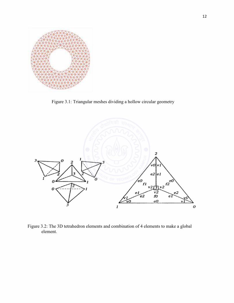
12
Figure 3.1: Triangular meshes dividing a hollow circular geometry
Figure 3.2: The 3D tetrahedron elements and combination of 4 elements to make a global
element.

13
3.2Mathematical formulation for FEM in 2D and 3D EIT:
The DUT is meshed in 2D finite elements that are triangles. Each element has 3 vertices called
nodes.
The nodal voltages on each element can be approximated as:
₁ = 7₁8₁ + 9₁:₁ + ;₁3.1
₂ = 7₂8₂ + 9₂:₂ + ;₂3.2
₃ = 7₃8₃ + 9₃:₃ + ;₃3.3
₁,₂ and >represent the nodal voltages of vertices 1,2 and 3 of a single element.
7?,9?and ;? are the weights of interpolation function for i=1,2,3.
The voltage can be approximated based on the nodal voltages (₁,₂,₃ as
8, : = 1@ ∗ BC 8 :D 8D :D> 8> :>E + C1 :1 D :D1 > :>E . 8 + C1 8 1 8D D1 8> >E . :F3.4
where, D= 2*GH
GH=Area of the element (triangle) =C1 8 :1 8D :D1 8> :>E The total no of nodes=N
And total no of elements=K
The potential of a linear 2D element can be expressed as:
8, : = 07?. 8 +>? 9? . : + ;. ?3.5

14
The potential inside of a 3D element can also be written as:
8, :, I = 0 7? . 8 + 9? . : + ;? . I + $?. ? 3.6J?
The values of 7? ,9?,;?and$? for a 3D element are given in appendix A.2
So the potential inside an element can also be expressed as:
= K L?. ?? (3.7)
Ni‘s are called the shape function or interpolation function of the elements.
The shape functions or potential functions are chosen in that way so that
L?8? , :M =1 when N = O =0 when N ≠ O The sum of an interpolation function over an element is equal to zero.
0L? = 0?
3.3 Finite Element implementation in solving equations:
Method of weighted residuals:
The method of weighted residuals is one of the finite element methods that has been used in EIT
to solve the partial differential equation. The fundamental equation of EIT is:

15
∇. ∇ = 0 In the MWR procedure we form a weight W such that the weighted integration of the EIT
equation becomes zero.
Let us consider, that the approximate solution of the FEM method is ₓ and the exact solution is
. From equation (2.1) it can be expressed that
∇. ∇ = 0and
∇. ∇ₓ ≈ 0
It is assumed that
∇. ∇ₓ = S(3.8)
The term S is called the residual. The method of weighted residuals refers that the weighted sum
or the integral of the residuals over all the elements can be zero if proper weight can be found.
The basic principle of MWR suggests thatfor an arbitrary ‘T’ the integral of the weighted
residual will be zero on the medium.
! TS$Ω = 03.9V
From Equations(2.1) and (3.8) it can be written that:
∇. ∇ₓ − ∇. ∇ = S3.10
Where T is a weight function which can be approximated as:

16
T = 0LM . XM 3.11YM
Here L? isinterpolation or shape function for weights and X?’s are the coefficients of the weight
function. @represents the dimension of the element. D=3 if the element is 2D and D=4 if the
element is 3D. Using Equations (3.10) and (3.11) it can be written that:
!T ∇. ∇ₓ$Ω = 03.12
From the basic equations of vector calculus it can be written that (Appendix: A)
Z[∇. T∇ₓ]$Ω = Z[∇ₓ . ∇T]$Ω(3.13)
From Gauss’s theorem it can be concluded that
!T∇ₓ. $Γ = ![∇ₓ . ∇T]$Ω3.14
This equation refers to the relationship the integral of dot product of two fields with the given
boundary condition. As it can be conferred that ∇].=]/ the equation (3.14) can be
written as:
![∇ₓ . ∇T]$Ω = !T ₓ $Γ3.15
The LHS of equation (3.16) represents the whole mesh that is the domain Ω and the RHS
represents the boundary conditions. The equation (3.16) can be formed for each element inside
the DUT. The integral will be over an element instead of the whole mesh. If the domain is
divided into ^ elements then we have ^ integrals to be solved to find the nodal voltage. For each

17
element a set of linear equation are formed, and these are combined to form the system equation
for the whole domain. From equations (3.8) and (3.12) the equation (3.16) can be rearranged for
an element _ (_ = 1, 2, ……… , ^). The conductivity of each element is assumed to be constant
along the element. This type of conductivity is called piecewise-constant conductivity.The
integral over the area of the _ element ` whose conductivity is assumed as`can be written
as:
! `∇."a ∇T = ` 0?>
? 0XM>
M G?M3.16
whereG?M is called the stiffness matrix of element ‘_’ and it is defined as:
G?M =Z ∇L? . ∇Ncd"a $Ω3.17L? and LM are the
shape functions of the FEM nodal voltage and weight function respectively for element _. From
this point onwards the FEM nodal voltage ₓ is considered as nodal voltage.
Thus a 3x3 matrix can be formed to solve the equations of a 2D element. Similarly a 4x 4 matrix
can be formed when 3D element is considered. The number of elements inside the DUT is K. To
solve the whole system equation the total no of equations needed are:
Kx3x3 for 2D FEM EIT and Kx4x4 for 3D FEM EIT.
Equation (3.18) represents the LHS of the equation (3.16). To form the equivalent for the RHS
the terms are required to be expanded in the FEM equations. The RHS can be represented as

18
!T ₓ $Γ = ` 0?>
? 0XM ! L? . ∇Nce . $Γ3.18>M
So, for an individual element _ the equation reduces to:
` 0?>
? 0G?M>
M = ` 00?Dgcd 3.19>M
>?
whereDgcd=Z L? . ∇Ncde . $Γ
The equation (3.20) is the final formulation of the 2D forward problem of EIT with the help of
finite element method. From equation (3.20) the global system matrix Gh can be formed by
combining the local stiffness matrix G` for each element. This global stiffness matrix is then
used to solve the forward problem for calculating the nodal voltages u from the injected current
pattern I depending upon which boundary condition has been implemented. The system matrix or
global stiffness matrix is also used to calculate the sensitivity or Jacobianmatrix which is used
for reconstruction .The forward problem can now be expressed as:
Gh.i = 3.20
Here i is the combined nodal voltage of all the nodes in the domain. Its dimension is N x 1.
Ghhas the dimension N x N and I be the injected current vector having dimension: N x 1.
The approach for constructing a global matrix from ^ local matrices is to construct a
connectivity matrix for the whole mesh based on the connectivity map of the elements. The
forward problem can be expressed as:
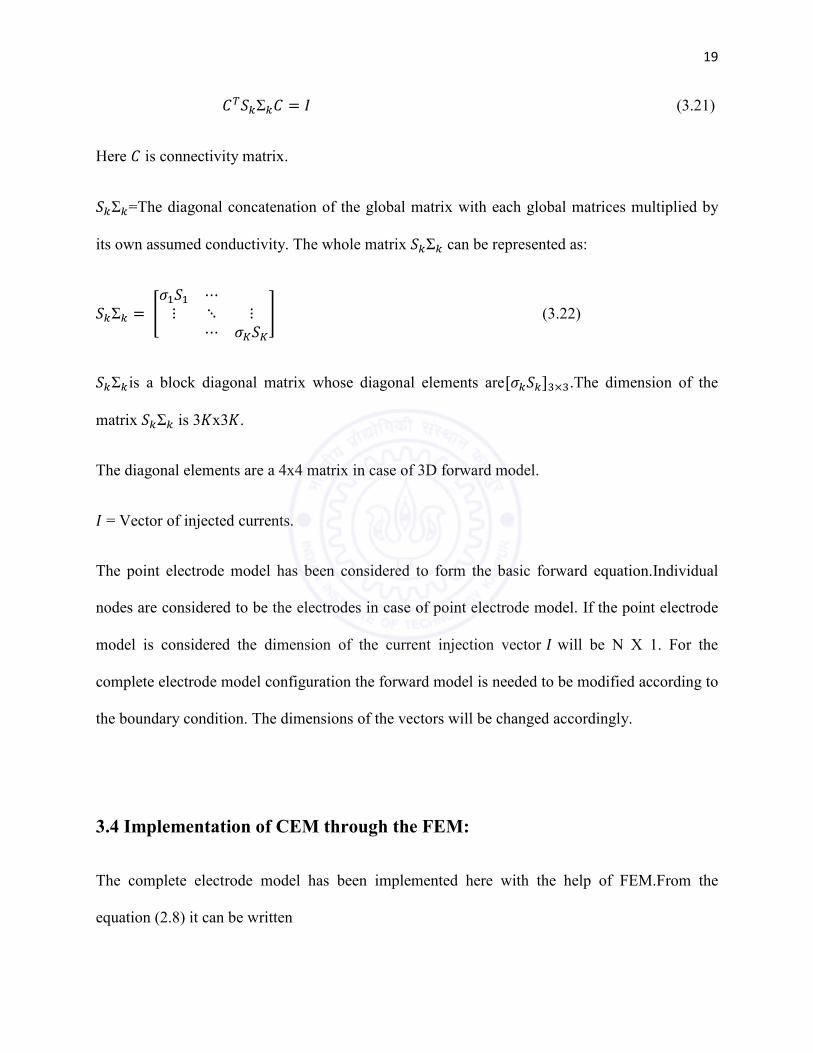
19
jkG`Σ`j = (3.21)
Here j is connectivity matrix.
G`Σ`=The diagonal concatenation of the global matrix with each global matrices multiplied by
its own assumed conductivity. The whole matrix G`Σ` can be represented as:
G`Σ` = CG ⋯⋮ ⋱ ⋮⋯ oGoE (3.22)
G`Σ`is a block diagonal matrix whose diagonal elements are[`G`]>×>.The dimension of the
matrix G`Σ` is 3^x3^.
The diagonal elements are a 4x4 matrix in case of 3D forward model.
= Vector of injected currents.
The point electrode model has been considered to form the basic forward equation.Individual
nodes are considered to be the electrodes in case of point electrode model. If the point electrode
model is considered the dimension of the current injection vector will be N Χ 1. For the
complete electrode model configuration the forward model is needed to be modified according to
the boundary condition. The dimensions of the vectors will be changed accordingly.
3.4 Implementation of CEM through the FEM:
The complete electrode model has been implemented here with the help of FEM.From the
equation (2.8) it can be written

20
= ∇. = 1' . − 3.23
So, the RHS of the FEM EIT equation (3.16) can be written as:
ZT∇. $Γ = K ZWrs . 1/Zs. − . $Ω′ (3.24)
Here Ω′ denotes the areas which are under the electrodes. This integration is done on the area
under each electrode from ( = 1, 2, ……… , ) and the summation has been taken. The RHS of
the equation (3.22) can be expanded to the FEM terms in the following expression:
0 Vl
L
l=1
! 1
Zl
u0 Nj
3
j=1
vjv dΓ - 0! 1
Zl
B0 Ni
3
i=1
uiFL
l=1
u0LM>
M XMv$Ω
Rearranging the terms the full governing equation of FEM EIT with CEM boundary conditions
for an element can be expressed as:
` K ?>? K XM>M Z ∇L?.∇LcdΩ) =
K K XM>M Z x# LM$Γ - K K ?>? K XM>M Z x# . yL? . LMz$Γ3.25
Equation (3.24) is valid for every test function X . So eliminating X from both sides of the
equation the final form of CEM equation is formed.
K `o K ? K yZ∇L? . ∇LcdΩz>M>? =
K Z 1/'"# . LM$Γ - K K ?>? K Z 1/'"#>M . yL?. LMz$ (3.26)
The current on the electrode is given by equation (2.3) as:

21
= ! ∇. $Γ"#
It can also be expressed as:
= ! 1/'"# . − $Γ = ! ' . $Γ"# − 0?>
? ! L?'"#. $Γ3.27
The contact impedance ' is assumed to be constant for each electrode and so it can be taken out
from the integral. The modified form of the electrode current can be expressed as:
= 1' . 3H. − 1' .0?>
? ! L?"#$Γ3.28
3H=Area under the electrode. In case of 2D it is the length of the electrode.
Combining equations (3.26) and (3.27) a new system matrix for 2D FEM EIT with CEM is
formed
This system matrix can be represented as:
3 + 3D 3>3>k 3J| i~ = 0 ~3.29
U= , D, > ……… . ×k = Matrix of all nodal voltages
V=, D, > … . ×k =Matrix of all voltages measured at the electrodes.
I = , D, > …… . ×= Matrix of the current injection vector.
0 = Null matrix with dimension=N × 1
22
The matrices 3, 3D, 3>, 3J are expressed as:
[3]?M = Z∇L?.∇LMdΩ
[3D]?M = K Z x# . L? . LM$Γi, j=1,2,3……..N
[3>]?M = −Z x# . L?$Γ i= 1, 2, 3……….N. j =1, 2, 3………L
[3J] = $N7 1' . 3H
Matrix 3 denotes the global stiffness matrix multiplied by the elemental conductivity matrix.
The matrix3is the system matrix ifpoint electrode model has been used, but since the CEM has
been used it has been modified with the addition of other matrices. Matrix 3 does not contain
any information about boundary conditions. Matrix 3D refers to the effects of contact
impedances on the system matrix. Matrix 3> represents the weights of voltages on the electrodes.
Matrix 3J adds the effect of contact impedance to the nodes which are situated under the
electrodes.
3.5 Calculation of Jacobian or Sensitivity matrix:
The reconstruction of the EIT images requires the calculation of the Jacobianor sensitivity matrix
which denotes the change of output voltage with change of conductivity.
The reconstruction of the EIT images requires the calculation of the Jacobian or sensitivity
matrix which denotes the change of output voltage with change of conductivity. The Jacobian or
sensitivity analysis expressed the rate of change of output voltage with respect to the change of
conductivity. This measure helps to determine whether a system is sensitive enough to reflect the
23
change of voltage when conductivity is changed even for a slightest amount. The expression for
the Jacobian is given by
= ?/M (3.30)
That implies change in the O voltage measurement when the the conductivity of the N element
has been changed.
The forward problem in EIT can be expressed as:
, + = 3.31
From the above equation the voltage matrix can be expressed as:
= , +. 3.32
Here , + is the admittance matrix which is both function of conductivity and position.
Taking derivative on both sides of equation (3.32) it can be written as:
= , +. , + . , +k . 3.33
The term is referred to as the Jacobian matrix or sensitivity matrix.
Adjoint method of calculating the Jacobian:
There is another method of calculating the Jacobian for the 2D and 3D EIT forward problem.
This method is called the adjoint method of calculation of Jacobian. The formula for Jacobian in
the adjoint method is given by:
24
N, _ = ?` = − ! ∇ . ∇ $Ω3.34
Here N is the N voltage measurement.`is the conductivity of the _ element. The terms
and denotes the voltage distribution inside the _ element when the injected
current pattern are the drive and measurement pattern. The integral is a surface integral when 2D
EIT problem is considered and is a volume integral when 3D EIT is considered.
The Jacobian matrix of dimension^ × where ^ is the number of elements and is the
number of measurement patterns. In this analysis both the 2D and 3D Jacobian matrix has been
calculated and they are verified with the Jacobian obtained through the EIDORS version 3.6
Jacobian calculation module ‘Jacobian_2d’ and ‘Jacobian_3d’ when the same injection and
measurement pattern has been analyzed.

25
Chapter 4
SIMULATED 2D AND 3D FORWARD PROBLEM OF EIT:
The forward problem of 2D and 3D EIT has been simulated here with the help of proper
boundary conditions. The solutions in the form of nodal voltages that is obtained are verified
with the solutions obtained from the standard software tool.
4.1 2D EIT Forward problem simulations:
The 2D EIT forward problem has been simulated on a circular geometry. The electrodes are
attached to the boundary of this circular domain. The radius of the circular DUT is considered to
be of 1unit.
The total number of electrodes attached = 16.
The electrodes are 2 dimensional so only their lengths are considered here.
The length of each electrode =0.1 unit.

26
The conductivity of the medium is considered to be homogenous and=1 unit.
Cross pattern of current injection has been done for the simulation.
Inter-electrode gap= D××. = 0.292unit
The currents that are injected are direct current in nature and the conductivity that is assumed to
have only real part.
The currents that are injected through electrodes are of magnitude =0.01mA
Value of contact impedance for electrodes: 60 Ohm-meter.
Number of nodes used in the FEM: 737
Number of elements for the FEM: 1385
The picture in Figure 4.1 shows the 2D EIT simulation on a circular geometry:
Figure 4.1: The 2D EIT forward problem simulation with the help of cross-pattern injection.
?= The current injected through one electrode.
=The output or sink current through diametrically opposite electrode.
V= The voltage measured differentially between two electrodes.
The number of measurements =208. The number of independent measurements=208/2=104.

27
Each electrode contains more than 2 nodes. The forward problem solution with point electrode
model gives the nodal voltage on each node of the DUT. The nodes which are under the
electrode are first determined. A weighted average based on the distance function is used to
measure the electrode voltages.
The voltage simulated on each electrode is calculated as:
= T + TDD + T>> + ⋯4.1
The voltages , D, > are the nodal voltages of the nodes under the electrode. The weights
T,TD,T> are the weights based on the distances of the nodes in the electrode. For example, if
there are three nodes under an electrode the node which is at middle will have higher weight than
the nodes on the terminal.
4.2 The 3D EIT Forward problem Simulation:
The 3D EIT forward problem is done on a spherical domain. A sphere of radius unity is
considered. The sphere is sub-divided into tetrahedron elements. Electrodes are placed on some
particular positions of the sphere. Two electrodes are used here for the simulation purpose. The
two electrodes are placed in the position (0, 0,1) and (0, 0, -1).
The nodal voltages are obtained by solving the 3D forward model. The conductivity is assumed
to be constant throughout the material and equal to 10.
The solutions of the nodal voltages that are obtained from the forward model simulation are
compared to the results obtained from the analytical solution of EIT equation on spherical
domain.

28
Chapter 5
RESULTS AND DISCUSSIONS:
This chapter presents the comparative analysis between the nodal voltages obtained from the 2D
and 3D FEM EIT to the solutions obtained from the standard software tool EIDORS and the
analytical solution. This analysis proves the accuracy and closeness of solution between the finite
element based method and other methods available. In this work two cases have been considered.
Case I: A circular geometry of unit radius is considered. Meshing is done on the geometry with
varying mesh size.
Currents are injected from the boundary nodes.The magnitude of applied current is equal to 1
mili-Ampere. The analysis is done here on different mesh sizes and then the nodal voltages
obtained are compared to that of analytic solution and EIDORS solution. Comparative analysis

29
on simulated voltage have been done for different mesh size and based on that calculation an
optimal mesh size has been chosen. Background conductivity is chosen to be 10unit.
Figure 5.1: The 2D FEM Meshing of a circular geometry
Case II: The 3D FEM EIT equation is solved on a spherical domain. Two electrodes have been
attached to that spherical domain. One is for injection of current and another is for sink. The
radius of this spherical domain is 1 unit. The electrodes are attached in the vertices (0,0,1) and
(0,0,-1) respectively. The mesh size used is 0.08. Number of nodes are 4385 and Number of
elements are 23000.The solution is then compared with the analytic solution of 3D EIT equation
for verification. Figure 5.2 describes the geometry of operation for 3D FEM EIT.

30
Figure 5.2: The 3D Elements dividing a spherical geometry with radius 1
(a) Mesh Size=0.06

31
(b)Mesh Size=0.07
(c)Mesh Size=0.08
Figure 5.3: Comparison of Nodal Voltages with EIDORS solution for different mesh size (a)
Mesh size=0.06 (b) Mesh size=0.07 and (c) Mesh size=0.08
Figure 5.3 shows the comparative analysis between Nodal Voltages obtained from 2D FEM EIT
with different mesh resolution or size to standard software solution.

32
(a) Mesh Size=0.08
(b) Mesh Size=0.07
(c) Mesh Size=0.06

33
Figure 5.4: Nodal Voltage distribution within a circular geometry for different mesh sizes (a)
0.08 (b) 0.07 and (c) 0.06.
Table 5.1: Comparison between different Mesh sizes for 2D FEM:
S.
No
Mesh
Dimension Average Error[
. − /] Number of
Nodes
Number
of
Elements
1 0.06 0.0186 1008 1910
2 0.07 0.0297 737 1385
3 0.08 0.0359 562 1045
Table 5.1 shows the corresponding analysis of average error and number of nodes and elements
for each mesh size. This comparison proves thatwith the decrease of mesh dimension and
increase in the number of mesh nodes or elements the average error tends to decrease. Increase in
the number of elements also suggests greater calculation complexity and greater run time. So, a
trade-off between calculation complexity and accuracy has to be chosen. In this case of circular
geometry with radius 1 unit the mesh dimension 0.07 seems to be a reasonable solution.
34
Figure 5.5: Comparison between 2D FEM EIT solutions of Nodal Voltages to that obtained
from Analytic solution.
Figure 5.5 shows the comparative analysis between the 2D FEM EIT nodal voltages and the
analytic solution. The mesh dimension of 0.07 has been used here for comparison. The average
error in thiscase is:
Average Error= 0.0273.
This analysis proves the closeness of solutions between 2D FEM analysis, standard software tool
analysis and analytic solution of 2D EIT equation.
The average error pattern for 2D and 3D EIT forward problem proves that the error margin is
less in case of 3D analysis but the calculation complexity resources (memory) usage is very high.
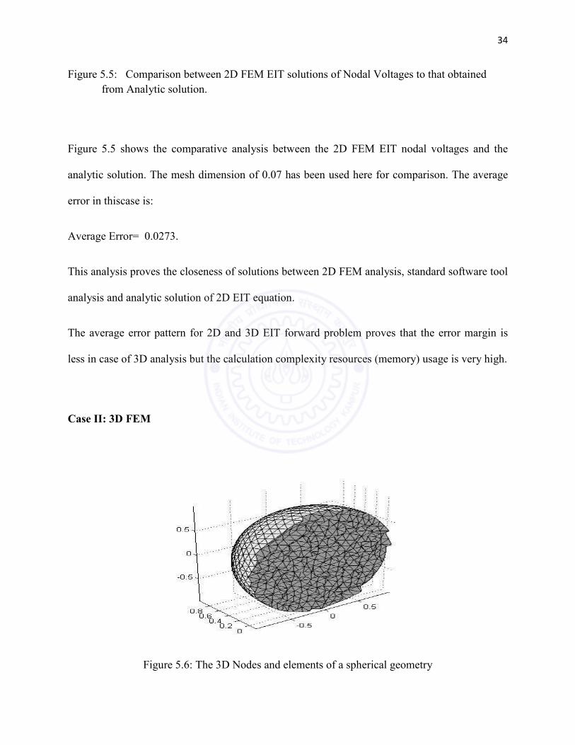
Case II: 3D FEM
Figure 5.6: The 3D Nodes and elements of a spherical geometry
35
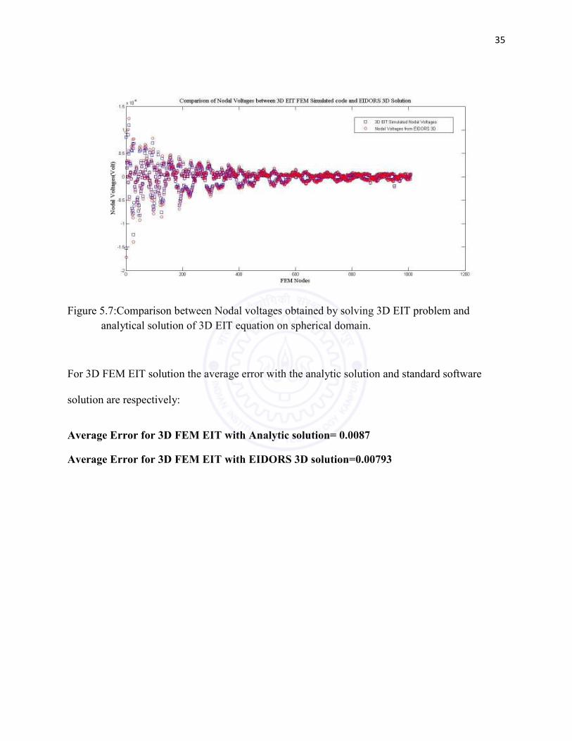
Figure 5.7:Comparison between Nodal voltages obtained by solving 3D EIT problem and
analytical solution of 3D EIT equation on spherical domain.
For 3D FEM EIT solution the average error with the analytic solution and standard software
solution are respectively:
Average Error for 3D FEM EIT with Analytic solution= 0.0087
Average Error for 3D FEM EIT with EIDORS 3D solution=0.00793

36
Chapter 6
CONCLUSION:
The forward problem of Electrical Impedance Tomography has been implementedand validated
here. EIT forward problem analysis can lead to the following conclusions:
1) The present work in this thesis establishes and validates the 2D and 3D forward model of
Electrical Impedance Tomography.
2) The results obtained in this thesis prove the correctness of the solutions of both analytic and
that obtained from the EIDORS software tools [8].
3)The analytic solutions that has been done here solves the EIT partial differential equation in
some particular geometry like circular in 2D and spherical in 3D[9 and 10].
4) The Jacobian for both 2D and 3D EIT has been calculated and compared to Jacobian obtained
from EIDORS 2D and 3D. The results differ very small in the order of 107
.This proves the
accuracy of the calculation.

37
REFERENCES:
[1] Cheney M., Issacson D., Newell J.C. Electrical Impedance Tomography.1999 Society for
Industrial and Applied Mathematics, Vol. 41. pp. 85-101
[2] Adler A. and Guardo R. “Electrical Impedance Tomography: regularized imaging and
contrast detection”, IEEE Transaction. Med-Imaging, Vol.15. pp. 170-179
[3] Bera T.K and Nagaraju J. 2009 FEM based Forward-solver for studying the Forward
problem of Electrical Impedance Tomography with a practical biological phantom;Advance
computing conference, 2009 IACC 2009.IEEE International,pp.1375-1381.
[4] Adler A and Lionheart WRB. “Uses and abuses of EIDORS an extensible software for
EIT”, Physiol Meas.
[5] Polydorides N, Lionheart WRB. “A MATLAB based toolkit for three-dimensional Electrical
Impedance Tomography: A contribution to the EIDORS project, Measurement Science and
Technology”, IoP Publishing, December 2002,Vol. 13, no. 12, pp. 1871-1883,.
[6] Vauhkonen M, Lionheart WRB, Heikkinen LM, Vauhkonen PJ, Kaipio JP: A MATLAB
package for the EIDORS project to reconstruct two-dimensional EIT images. PhysiolMeas
2001, pp.107-111.
[7] Gomez-Laberge, C and Adler, A. Imaging of electrode movement and conductivity change
in Electrical Impedance Tomography. May 2006, Electrical and Computing Engineering, 2006,
CCECE’06,Canadian conference –on, pp. 975-978.

38
[8] SaeedizadehN., KermaniSaeed., RabbaniH. “A Comparison between the hp-Version of Finite
Element Method with EIDORS for Electrical Impedance Tomography”Journal of Medical
Signals & Sensors,2011Vol.1. pp. 215-221.
[9] Akdogan K.E., YilmazA. and Saka, B. “Analysis of forward problem for elliptical geometry
in EIT by using analytical and finite element methods”, Circuits and Systems,2003 IEEE 46th
Midwest Symposium Vol.1. pp. 372-375
[10] GuizhiXu.,Huanli Wu, Shuo Yang, Shuo Liu , Ying Li. 3-D Electrical Impedance
Tomography Forward Problem With Finite Element Method. IEEE TRANSACTIONS ON
MAGNETICS, VOL. 41, NO. 5, MAY 2005. pp. 1832-1836

39
APPENDIX A:
A.1:
∇. = 0 When there is no charge accumulated in the medium considered.
=
= −∇
These equations form the basic equation of EIT that is:
∇. ∇ = 0
A.2:
3D EIT Calculations:
The voltage inside a 3D element in EIT can be expressed as
8, :, I = 7. 8 + 9. : + ;. I + $
(a,b,c,d) are constants. (x ,y,z) the vertices of the point.
The vertices of a 3D element be = (8, :, I ,8D, :D, ID,8>, :>, I>,8J, :J, IJ
D>J= 79;$k . 18:I
18D:DID18>:>I>
18J:JIJ
Solving the equation by Kramer’s rule the values of a, b ,c ,d can be found.
The values of the co-efficients (a,b,c,d) can be expressed as:
7 = 7. + 7D. D + 7>. > + 7J. J/6H
The values of 7,7D,7>,7J are obtained from solving the above equation.

40
Similarly the values of 9, ;and $ can be expressed as the same way:
The local stiffness matrix of _ element is given by:
G` = H36H . D>J88D8>8J
::D:>:JIIDI>IJ
/ 111188D8>8J
::D:>:JIIDI>IJ
41
APPENDIX B:
Analytical Solution of 2D circular geometry:
The analytical solution on the 2D circular geometry can be obtained by solving the EIT
governing equation with boundary conditions on a circular geometry.
Two simple cases have been chosen and their corresponding solutions are discussed here. First
one is the analytic solution when the conductivity of the DUT is homogenous. The solution of
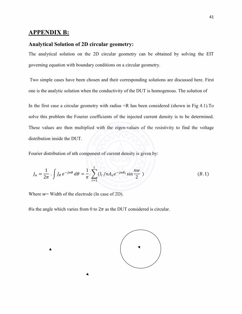
In the first case a circular geometry with radius =R has been considered (shown in Fig 4.1).To
solve this problem the Fourier coefficients of the injected current density is to be determined.
These values are then multiplied with the eigen-values of the resistivity to find the voltage
distribution inside the DUT.
Fourier distribution of nth component of current density is given by:
= 12 .! ¡ *M¡ $¢ = 1 .0 /3H*M¡# sin (2 ¦. 1
Where (= Width of the electrode (In case of 2D).
¢is the angle which varies from 0 to 2 as the DUT considered is circular.

42
The analytic value of voltage distribution within the DUT can be found as:
Case 1: When the DUT is homogenous.
¢ = K ∞∞H§¨©ªª (B.2)
Case 2: When the DUT is not homogenous
D¢ = 0 ∞
∞
*M¡ . 1 − ^SD1 + ^SD ¦. 3
Here ^ = − / + S=Radius of the inhomogeneity.
B.2 Analytic Solution of 3D EIT in Spherical domain:
In order to validate the 3D FEM code an analytic solution for 3D EIT has been done in the
spherical domain. The values of voltages obtained on a spherical object can be obtained
analytically by the following formula.
i« = 4 . 2S − log1 − «. 3 + S¯ − 4 2SD − log1 − «. ¦ + SD¯¦. 4
Here is the conductivity of the uniform sphere (Shown in Fig B.2). P denotes the distance from
the centre of the sphere to the point « where the voltage is being measured. 3, ¦denote the
distance of the current ( ) source and sink point. S is the distance between points 3 and «.

43
Similarly, SD is the distance between point « and point ¦. The current value and conductivity
value are kept the same to that of the FEM code so that they can be compared for validation.
P
AB B
Figure B.2: Analytical solution of 3D FEM